estimation of the global minimum variance portfolio in ... · portfolio, the global minimum...

Estimation of the Global Minimum Variance Portfolio in High Dimensions

Taras Bodnara, Nestor Parolyab and Wolfgang Schmidc 1

a Department of Mathematics, Stockholm University, Roslagsvagen 101, SE-10691 Stockholm, Sweden

b Department of Empirical Economics (Econometrics), Leibniz University Hannover, D-30167 Hannover, Germany

c Department of Statistics, European University Viadrina, PO Box 1786, 15207 Frankfurt (Oder), Germany

Abstract

We estimate the global minimum variance (GMV) portfolio in the high-dimensional case using

results from random matrix theory. This approach leads to a shrinkage-type estimator which

is distribution-free and it is optimal in the sense of minimizing the out-of-sample variance. Its

asymptotic properties are investigated assuming that the number of assets p depends on the sample

size n such that pn → c ∈ (0,+∞) as n tends to infinity. The results are obtained under weak

assumptions imposed on the distribution of the asset returns, namely it is only required the fourth

moments existence. Furthermore, we make no assumption on the upper bound of the spectrum

of the covariance matrix. As a result, the theoretical findings are also valid if the dependencies

between the asset returns are described by a factor model which appears to be very popular in

financial literature nowadays. This is also well-documented in a numerical study where the small-

and large-sample behavior of the derived estimator are compared with existing estimators of the

GMV portfolio. The resulting estimator shows significant improvements and it turns out to be

robust to the deviations from normality.

JEL Classification: G11, C13, C14, C58, C65

Keywords: global minimum variance portfolio, large-dimensional asymptotics, covariance matrix esti-

mation, random matrix theory.

1 Introduction

Since Markowitz (1952) presented his seminal work about portfolio selection, this topic has become a

very fast growing branch of finance. One of Markowitz’s ideas was the minimization of the portfolio

variance subject to the budget constraint. This approach leads to the well-known and frequently used

portfolio, the global minimum variance portfolio (GMV). There is a great amount of papers dealing

with the GMV portfolio (see, e.g., Jagannathan and Ma (2003), Ledoit and Wolf (2003), Okhrin and

Schmid (2006), Kempf and Memmel (2006), Bodnar and Schmid (2008), Frahm and Memmel (2010)

among others). We remind that the GMV portfolio is the unique solution of the following optimization

1Corresponding author. E-mail address: [email protected]

1

arX

iv:1

406.

0437

v2 [

q-fi

n.ST

] 1

3 N

ov 2

015

problem

w′Σnw→ min subject to w′1 = 1 , (1.1)

where w = (w1, . . . , wp)′ denotes the vector of portfolio weights, 1 is a suitable vector of ones, and

Σn stands for the covariance matrix of the asset returns. Note that in our paper p is a function of

the sample size n and thus the covariance matrix depends on n as well. This is shown by the index n.

The solution of (1.1) is given by

wGMV =Σ−1n 1

1′Σ−1n 1. (1.2)

The GMV portfolio (1.2) has the smallest variance over all portfolios. It is also used in multi-period

portfolio choice problems (see, e.g., Brandt (2010)). Although this portfolio possesses several nice

theoretical properties, some problems arise when the uncertainty about the parameters of the asset

return distribution is taken into account. Indeed, we do not know the population covariance matrix in

practice and, thus, it has to be suitably estimated. Consequently, the estimation of the GMV portfolio

is strongly connected with the estimation of the covariance matrix of the asset returns.

The traditional estimator is a commonly used possibility for the estimation of the GMV portfolio

(1.2). This traditional estimator is constructed by replacing in (1.2) the covariance matrix Σn by its

sample counterpart Sn. Okhrin and Schmid (2006) derived the distribution of the traditional estimator

and studied its properties under the assumption that the asset returns follow a multivariate normal

distribution, whereas Kempf and Memmel (2006) analyzed its conditional distributional properties.

Furthermore, Bodnar and Schmid (2009) derived the distribution of the main characteristics of the

sample GMV portfolio, namely its variance and its expected return.

The traditional estimator is not a bad choice if the number of assets p is fixed and it is significantly

smaller than the number of observations n in the sample. This case is often used in statistics and it

is called standard asymptotics (see, Le Cam and Yang (2000)). In that case the traditional estimator

is a consistent estimator for the GMV portfolio and it is asymptotically normally distributed (Okhrin

and Schmid (2006)). As a result, for a small fixed dimension p ∈ {5, 10, 15} we can use the sample

estimator but it is not fully clear what to do if the number of assets in the portfolio is extremely large,

say p ∈ {100, 500, 1000}, comparable to n. Here we are in the situation when both the number of

assets p and the sample size n tend to infinity. This double asymptotics has an interpretation when

p and n are of comparable size. More precisely, when p/n tends to a concentration ratio c > 0. This

type of asymptotics is known as high-dimensional asymptotics or ”Kolmogorov” asymptotics (see, Bai

and Silverstein (2010)). Under the high-dimensional asymptotics the traditional estimator behaves

very unpredictable and it is far from the optimum one. It tends to underestimate the risk (see, El

Karoui (2010), Bai and Shi (2011)). In general, the traditional estimator is worse for larger values

of the concentration ratio c. Imposing the assumption of a factor structure on the asset returns this

problem was resolved in an efficient way by Bai (2003), Fan et al. (2008), Fan et al. (2012), Fan et

al. (2013), etc. Nevertheless, if the factor structure is not present the question of high-dimensionality

remains open.

Further estimators for the weights of the GMV portfolio have been proposed in this situation.

DeMiguel et al. (2009) suggested to involve some additional portfolio constraints in order to avoid

2

the curse of dimensionality. On the other hand, shrinkage estimators can be used which are biased

but can significantly reduce the risk of the portfolio by minimizing its mean-square error. The general

shrinkage estimator is a convex combination of the traditional estimator and a known target (for

the GMV portfolio it can be the naive equally weighted portfolio). They were first considered by

Stein (1956). Recently, various authors showed that shrinkage estimators for the portfolio weights

indeed lead to better results (see, e.g., Golosnoy and Okhrin (2007), Frahm and Memmel (2010)). In

particular, Golosnoy and Okhrin (2007) considered a multivariate shrinkage estimator by shrinking

the portfolio weights themselves but not the whole sample covariance matrix. The same idea was used

by Frahm and Memmel (2010) who constructed a feasible shrinkage estimator for the GMV portfolio

which dominates the traditional one. There are several problems with these estimators: first, the

normal distribution is usually imposed; second, dominating does not mean optimal; and third, the

large dimensional behavior (large p and large n) seems not to be acceptable.

The aim of the paper is to derive a feasible and simple estimator for the GMV portfolio which

is optimal, in some sense, for small and large sample sizes and which is distribution-free as well.

For that purpose we construct an optimal shrinkage estimator, study its asymptotic properties and

estimate unknown quantities consistently. The estimator is obtained using random matrix theory, a

fast growing branch of probability theory. The main result of this theory was proved by Marcenko and

Pastur (1967) and further extended under very general conditions by Silverstein (1995). Nowadays it

is called Marcenko-Pastur equation. Its importance arises in many areas of science because it shows

how the real covariance matrix and its sample estimate are connected with each other. Knowing this

information we can build suitable estimators for high-dimensional quantities.

The rest of the paper is organized as follows. In Section 2 we present a shrinkage estimator for the

GMV portfolio which is optimal in terms of minimizing the out-of-sample variance. The asymptotic

behavior of the resulting shrinkage intensity is investigated for c < 1 in Section 2.1 and in case of c > 1

in Section 2.2 where it is shown that the shrinkage intensity tends almost surely to a deterministic

quantity when both the sample size and the portfolio dimension increase. This result allows us to

determine an oracle estimator of the GMV portfolio, while the corresponding bona fide estimator is

presented in Section 2.3. In Section 3 we provide a simulation study for different values of c ∈ (0,+∞)

and under various distributional assumptions imposed on the data generating process. Here, the

performance and the convergence rate of the derived shrinkage estimator are compared with existing

estimators of the GMV portfolio. The results of our empirical study are given in Section 4 where

we apply the suggested estimator as well as the existing estimators to real data consisting of returns

on assets included in the S&P 500 (Standard & Poor’s 500) index. Section 5 summarizes all of the

obtained results. The lengthy proofs are moved to the appendix (Section 6).

2 Optimal shrinkage estimator for the GMV portfolio

Let Yn = (y1,y2, ...,yn) be the p×n data matrix which consists of n vectors of the returns on p ≡ p(n)

assets. Let E(yi) = µn and Cov(yi) = Σn for i ∈ 1, ..., n. We assume that p/n → c ∈ (0,+∞) as

n → ∞. This type of limiting behavior is also denoted as ”large dimensional asymptotics” or ”the

Kolmogorov asymptotics”. In this case the traditional estimators perform poor or even very poor and

3

tend to over/underestimate the unknown parameters of the asset returns, i.e., the mean vector and

the covariance matrix.

Throughout the paper it is assumed that it exists a p × n random matrix Xn which consists of

independent and identically distributed (i.i.d.) real random variables with zero mean and unit variance

such that

Yn = µn1′ + Σ

12nXn . (2.1)

It is noted that the observation matrix Yn consists of dependent rows although its columns are inde-

pendent. The assumption of the independence of the columns can further be weakened by controlling

the growth of the number of dependent entries, while no specific distributional assumptions are im-

posed on the elements of Yn (see, Friesen et al.(2013)).

The two main assumptions which are used throughout the paper are

(A1) The covariance matrix of the asset returns Σn is a nonrandom p-dimensional positive definite

matrix.

(A2) The elements of the matrix Xn have uniformly bounded 4 + ε moments for some ε > 0.

These two regularity conditions are very general and they fit many practical situations. The as-

sumption (A1) is common for financial and statistical problems. It does not impose a strong restriction

on the data-generating process, whereas the assumption (A2) is purely technical. Moreover, it seems

to influence only the convergence rate of the proposed estimator (see, e.g. Rubio et al. (2012)).

The sample covariance matrix is given by

Sn =1

nYn(I− 1

n11′)Y′n =

1

nΣ

12nXn(I− 1

n11′)X′nΣ

12n , (2.2)

where the symbol I stands for the identity matrix of an appropriate dimension.

2.1 Oracle estimator. Case c < 1

The traditional estimator for the GMV portfolio is obtained by replacing the unknown population

covariance matrix Σn in (1.2) by the estimator (2.2) . This leads to

wGMV =S−1n 1

1′S−1n 1. (2.3)

Next, we derive the optimal shrinkage estimator for the GMV portfolio weights by optimizing with

respect to the shrinkage parameter αn and fixing some target portfolio bn. Its distributional properties

are studied after that. The general shrinkage estimator (GSE) for c ∈ (0, 1) is defined by

wGSE = αnS−1n 1

1′S−1n 1+ (1− αn)bn with b′n1 = 1 (2.4)

where bn ∈ Rp is a given nonrandom (or random but independent of the actual observation vector

yn, i.e., the last column of Yn) vector. No assumption is imposed on the shrinkage intensity αn which

is the object of our interest. The aim is to find the optimal shrinkage intensity αn. for a given target

4

portfolio bn which minimizes the out-of-sample risk

L = ||Σ12n (wGSE(αn)−wGMV )|| = (wGSE(αn)−wGMV )′Σn(wGSE(αn)−wGMV ) , (2.5)

(see, e.g., Frahm and Memmel (2010), Rubio et al. (2012)). The loss function (2.5) can be rewritten

as

L = w′GSE(αn)ΣnwGSE(αn)− σ2GMV , (2.6)

where σ2GMV =1

1′Σ−1n 1is the population variance of the GMV portfolio and w′GSE(αn)ΣnwGSE(αn)

is known as the out-of-sample variance of the portfolio with the weights wGSE(αn).

Using (2.4) we want to solve the following optimization problem

minαn

L = minαn

α2nσ

2S + 2αn(1− αn)

1

1′S−1n 11′S−1n Σnbn + (1− αn)2b′nΣnbn − σ2GMV , (2.7)

where

σ2S =1′S−1n ΣnS

−1n 1

(1′S−1n 1)2(2.8)

is the out-of-sample variance of the traditional estimator for the GMV portfolio weights. Taking the

derivative of L with respect to αn and setting it equal to zero we get

∂L

∂αn= αnσ

2S + (1− 2αn)

1′S−1n Σnbn

1′S−1n 1− (1− αn)b′nΣnbn = 0 . (2.9)

From the last equation it is easy to find the optimal shrinkage intensity α∗n given by

α∗n =

b′nΣnbn −1′S−1n Σnbn

1′S−1n 1

σ2S − 21′S−1n Σnbn

1′S−1n 1+ b′nΣnbn

=

(bn −

S−1n 1

1′S−1n 1

)′Σnbn(

bn −S−1n 1

1′S−1n 1

)′Σn

(bn −

S−1n 1

1′S−1n 1

) . (2.10)

In order to ensure that α∗n is the minimizer of (2.7) we calculate the second derivative of L which

has to be positive. It holds that

∂2L

∂α2n

= σ2S − 21′S−1n Σnbn1

1′S−1n 1+ b′nΣnbn =

(bn −

S−1n 1

1′S−1n 1

)′Σn

(bn −

S−1n 1

1′S−1n 1

)> 0 (2.11)

almost surely. The last inequality is always true because of the positive definiteness of the matrix Σn

and the fact that bn =S−1n 1

1′S−1n 1with probability zero.

In Theorem 2.1 we show that the optimal shrinkage intensity α∗n is almost surely asymptotically

equivalent to a nonrandom quantity α∗ ∈ [0, 1] under the large-dimensional asymptoticsp

n→ c ∈

(0, 1). Let σbn = b′nΣnbn be the variance of the target portfolio and let

Rbn =σ2bn− σ2GMV

σ2GMV

be the relative loss of the target portfolio bn.

5

Theorem 2.1. Assume (A1)-(A2). Let 0 < Ml ≤ σ2GMV ≤ σ2bn≤ Mu < ∞ for all n. Then it holds

that

α∗na.s.−→ α∗ =

(1− c)Rb

c+ (1− c)Rbfor

p

n→ c ∈ (0, 1) as n→∞ , (2.12)

where Rb is the limit of Rbn. Additionally, the out-of-sample variance σ2S of the traditional estimator

for the GMV portfolio possesses the following asymptotic behavior

σ2Sa.s.−→ 1

1− cσ2GMV for

p

n→ c ∈ (0, 1) as n→∞ . (2.13)

The proof of Theorem 2.1 is given in the Appendix. Theorem 2.1 provides us important information

about the optimal shrinkage estimator of the GMV portfolio. Especially, the application of Theorem

2.1 immediately leads to consistent estimators for α∗n, σ2GMV , and σ2S which are presented in Section

2.3 below. It is remarkable to note that the assumption 0 < Ml ≤ σ2GMV ≤ σ2bn≤Mu <∞ is natural

for financial markets. It ensures that the population variance of the GMV portfolio has a lower bound

which is in-line with the Capital Asset Pricing Model since the portfolio variance cannot be smaller

than the market risk (see, e.g., Elton et al. (2007, Chapter 7)). Moreover, the assumption of the

boundedness of the variance of the target portfolio σ2bnis also well acceptable because it makes no

sense to shrink to a portfolio with infinite variance. Most importantly, this condition also holds even

if the largest eigenvalue of the covariance matrix is unbounded. Such a situation is present if the asset

returns follow a factor model which is a very popular approach in financial literature nowadays (see,

e.g., Fan et al. (2008), Fan et al. (2012)). It is worth pointing out that the same result is true if we

assume instead of 0 < Ml ≤ σ2GMV ≤ σ2bn≤ Mu < ∞ the boundedness of the spectral norm of the

population covariance matrix, i.e., the uniformly bounded maximum eigenvalue of Σn.

The answer on the question about the performance of the traditional and the optimal shrinkage

estimator for the GMV portfolio is given in Corollary 2.1.

Corollary 2.1. (a) Under the assumptions of Theorem 2.1, we get for the relative loss of the tradi-

tional estimator for the GMV portfolio

RS =σ2S − σ2GMV

σ2GMV

a.s.−→ c

1− cfor

p

n→ c ∈ (0, 1) as n→∞ . (2.14)

(b) Under the assumptions of Theorem 2.1, we get for the relative loss of the optimal shrinkage

estimator for the GMV portfolio

RGSE =wTGSEΣnwGSE − σ2GMV

σ2GMV

a.s.−→ (α∗)2c

1− c+(1−α∗)2Rb for

p

n→ c ∈ (0, 1) as n→∞ .

(2.15)

Corollary 2.1 is a straightforward consequence of Theorem 2.1. Moreover, its first part generalizes

the result of Frahm and Memmel (2010, Theorem 7) to an arbitrary distribution of the asset returns.

Using Corollary 2.1(a) we can plot the behavior of the relative loss of the traditional estimator for the

GMV portfolio as a function of the concentration ratio c only, while the relative loss of the optimal

6

shrinkage portfolio additionally depends on the relative loss of the target portfolio. Furthermore, from

both parts of Corollary 2.1 we get

RGSEa.s.−→ (α∗)2RS + (1− α∗)2Rb for

p

n→ c ∈ (0, 1) as n→∞ ,

i.e., the relative loss of the optimal shrinkage estimator for the GMV portfolio can asymptotically be

presented as a linear combination of the relative loss of the traditional estimator and the relative loss

of the target portfolio. Because α∗ → 0 as c→ 1−2 and

(α∗)2c

1− c=

(1− c)cR2b

(c+ (1− c)Rb)2→ 0 as c→ 1− ,

we get that RGSE → Rb ≤ Mu−MlMl

as c → 1−, whereas the relative loss of the traditional estimator

tends to infinity.

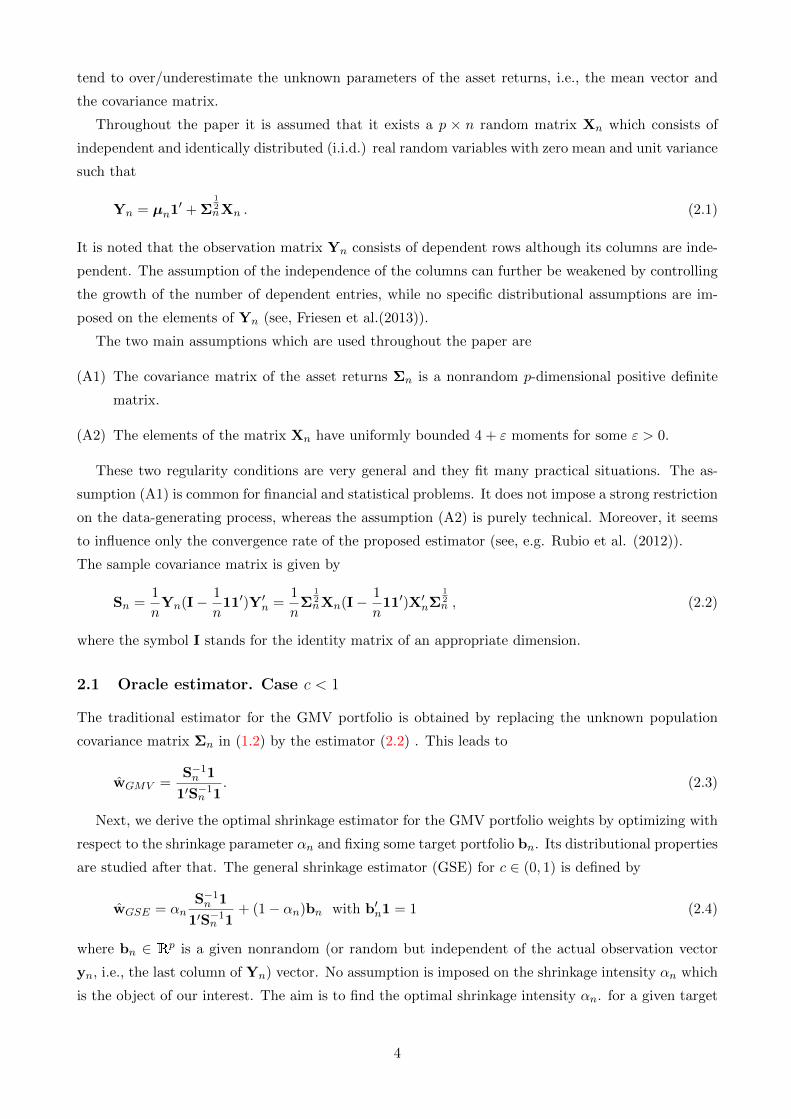
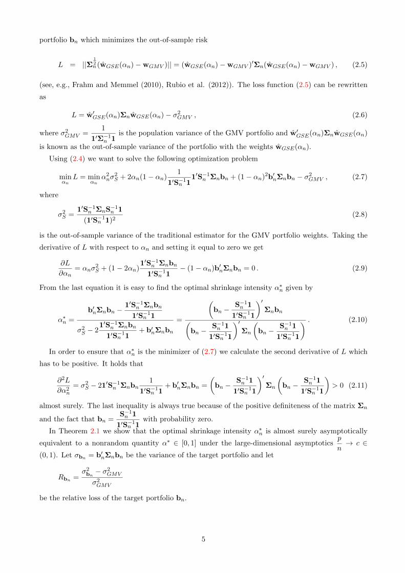
Figure 1 presents the behavior of the traditional and the proposed oracle estimators of the GMV

portfolio weights for different values of c ∈ (0, 1). The covariance matrix Σn is taken as a 200× 200-

dimensional matrix where we have taken 20% of the eigenvalues equal to 3, 40% equal to 1, and 40%

equal to 0.5. The matrix of eigenvectors V = (v1, . . . ,vp)′ is generated from the Haar distribution3

The target portfolio is chosen as the equally weighted portfolio, i.e. bn = 1/p1. In the figure we

observe that the asymptotic relative loss of the traditional estimator for the GMV portfolio has a

singularity point at one. The loss of the traditional estimator is relatively small up to c = 0.2 but

thereafter, as p/n→ 1, it rises hyperbolically to infinity. In contrast to the traditional estimator of the

GMV portfolio weights, the suggested optimal shrinkage estimator has a constant asymptotic relative

loss which is always smaller than 0.5. This result is in-line with the theoretical findings discussed

around Corollary 2.1.

Figures 1 and 2 above here

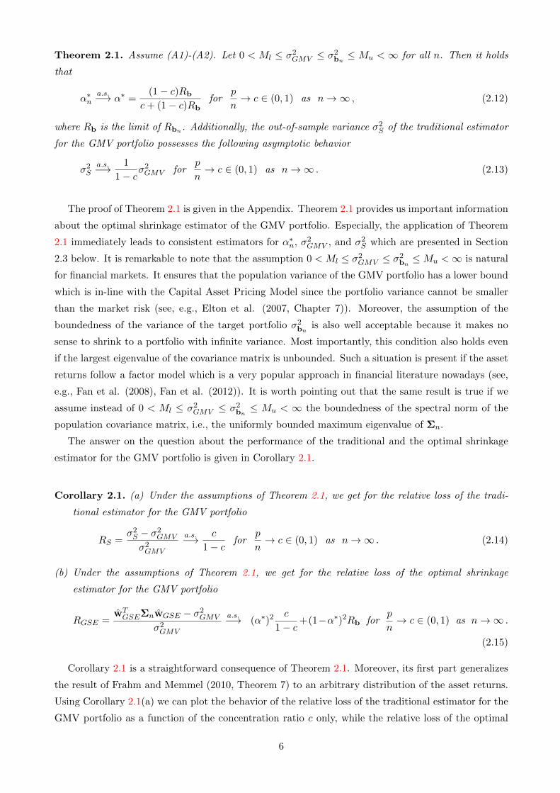
In Figure 2 we show the asymptotic behavior of the optimal shrinkage intensity α∗ as a function of

the concentration ratio c ∈ (0, 1). The target portfolio bn and the covariance matrix Σn are the same

as in Figure 1. In the interval c ∈ (0, 1) the optimal shrinkage intensity α∗ is a nonlinearly decreasing

(in a convex manner) function of the concentration ratio c. We observe that the optimal α∗ tends to

zero as c approaches one and, thus, in the limiting case the only optimal choice would be the target

portfolio bn.

2.2 Oracle estimator. Case c > 1

In case c > 1, the sample covariance matrix Sn is singular and its inverse does not exist anymore.

Thus, we first have to find a reasonable replacement for S−1n . For the oracle estimator of the GMV

portfolio weights we use the following generalized inverse of the sample covariance matrix Sn

S∗n = Σ−1/2n (XnX′n)+Σ−1/2n , (2.16)

2Further in paper, c → 1− and c → 1+ denote the left and right limits to the point 1, respectively.3If V has a Haar measure over the orthogonal matrices, then for any unit vector x ∈ Rp, Vx has a uniform distribution

over the unit sphere Sp = {x ∈ Rp; ||x|| = 1}.

7

where ′+′ denotes the Moore-Penrose inverse. It can be shown that S∗n is the generalized inverse

satisfying S∗nSnS∗n = S∗n and SnS

∗nSn = Sn.4 Obviously, in case c < 1 the generalized inverse S∗n

coincides with the usual inverse S−1n . Moreover, if Σn is proportional to the identity matrix then

S∗n coincides with the Moore-Penrose inverse S+n calculated for Sn. It has also to be noted that S∗n

cannot be determined in practice since it depends on the unknown matrix Σn. In this section, it is

only used to determine an oracle estimator for the weights of the GMV portfolio, whereas the bona

fide estimator is constructed in Section 2.3.

Based on S∗n in (2.16), the oracle traditional estimator for the GMV portfolio in case c > 1 is first

constructed and it is given by

w∗GMV =S∗n1

1′S∗n1. (2.17)

Next, we determine the oracle optimal shrinkage estimator for the GMV portfolio weights expressed

as

w∗GSE = α+n

S∗n1

1′S∗n1+ (1− α+

n )bn with b′n1 = 1 . (2.18)

Similarly to Section 2.1, we deduce the optimal shrinkage intensity α+n given by

α+n =

b′nΣnbn −1′S∗nΣnbn

1′S∗n1

σ2S∗ − 21′S∗nΣnbn

1′S∗n1+ b′nΣnbn

=

(b− S∗n1

1′S∗n1

)′Σnb(

b− S∗n1

1′S∗n1

)′Σn

(b− S∗n1

1′S∗n1

) , (2.19)

where σ2S∗ = 1′S∗nΣnS∗n1/(1

′S∗n1)2 is the oracle out-of-sample variance of the traditional estimator for

the GMV portfolio. In Theorem 2.2 we present the asymptotic properties of the optimal α+n for c > 1.

Theorem 2.2. Assume (A1)-(A2). Let 0 < Ml ≤ σ2GMV ≤ σ2bn≤ Mu < ∞ for all n. Then it holds

that

α+n

a.s.−→ α+ =(c− 1)Rb

(c− 1)2 + c+ (c− 1)Rbfor

p

n→ c ∈ (1,+∞) as n→∞ , (2.20)

where Rb is the limit of Rbn. Additionally, we get for the oracle out-of-sample variance σ2S∗ of the

traditional estimator (2.17) for the GMV portfolio

σ2S∗a.s.−→ c2

c− 1σ2GMV for

p

n→ c ∈ (1,+∞) as n→∞ . (2.21)

The proof of Theorem 2.2 is given in the appendix. The asymptotic behavior of the relative loss

calculated for the traditional oracle estimator of the GMV portfolio as well as for the oracle optimal

shrinkage estimator is described in Corollary 2.2.

Corollary 2.2. (a) Under the assumptions of Theorem 2.2, we get for the relative loss of the oracle

traditional estimator for the GMV portfolio

R∗S =σ2S∗ − σ2GMV

σ2GMV

a.s.−→ c2 − c+ 1

c− 1for

p

n→ c ∈ (1,+∞) as n→∞ . (2.22)

4Note that S∗n is not equal to the Moore-Penrose inverse because it does not satisfy the conditions (S∗nSn)′ = S∗nSn and

(SnS∗n)′ = SnS

∗n. Nevertheless, in Section 2.3, where the bona fide estimator is constructed, we use the Moore-Penrose

inverse of Sn instead of S∗n in order to obtain a valuable approximation.

8

(b) Under the assumptions of Theorem 2.2, we get for the relative loss of the oracle optimal shrinkage

estimator for the GMV portfolio

R∗GSE =(w∗GSE)TΣnw

∗GSE − σ2GMV

σ2GMV

a.s.−→ (α+)2R∗S+(1−α+)2Rb forp

n→ c ∈ (0, 1) as n→∞ .

(2.23)

Similarly to the case c < 1, the relative loss of the optimal shrinkage estimator for the GMV

portfolio is a linear combination of the relative loss of the traditional estimator and the relative loss

of the target portfolio. Furthermore, if c→ 1+, the relative loss of the traditional estimator tends to

infinite5, whereas for the relative loss of the shrinkage estimator we get

R∗GSE →(c− 1)(c2 − c+ 1)R2

b

((c− 1)2 + c+ (c− 1)Rb)2+ (1− α+)2Rb = Rb as c→ 1+ ,

which is bounded from above by Mu−MlMl

, i.e., it is finite.

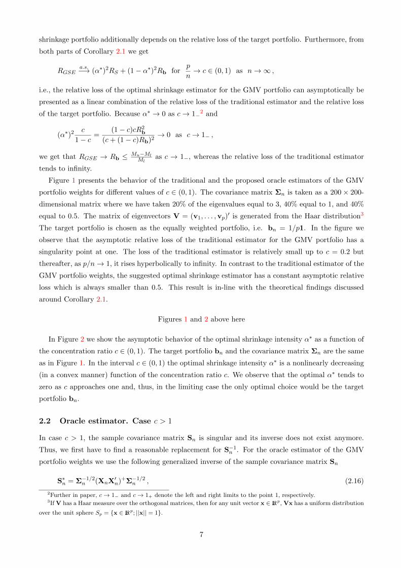
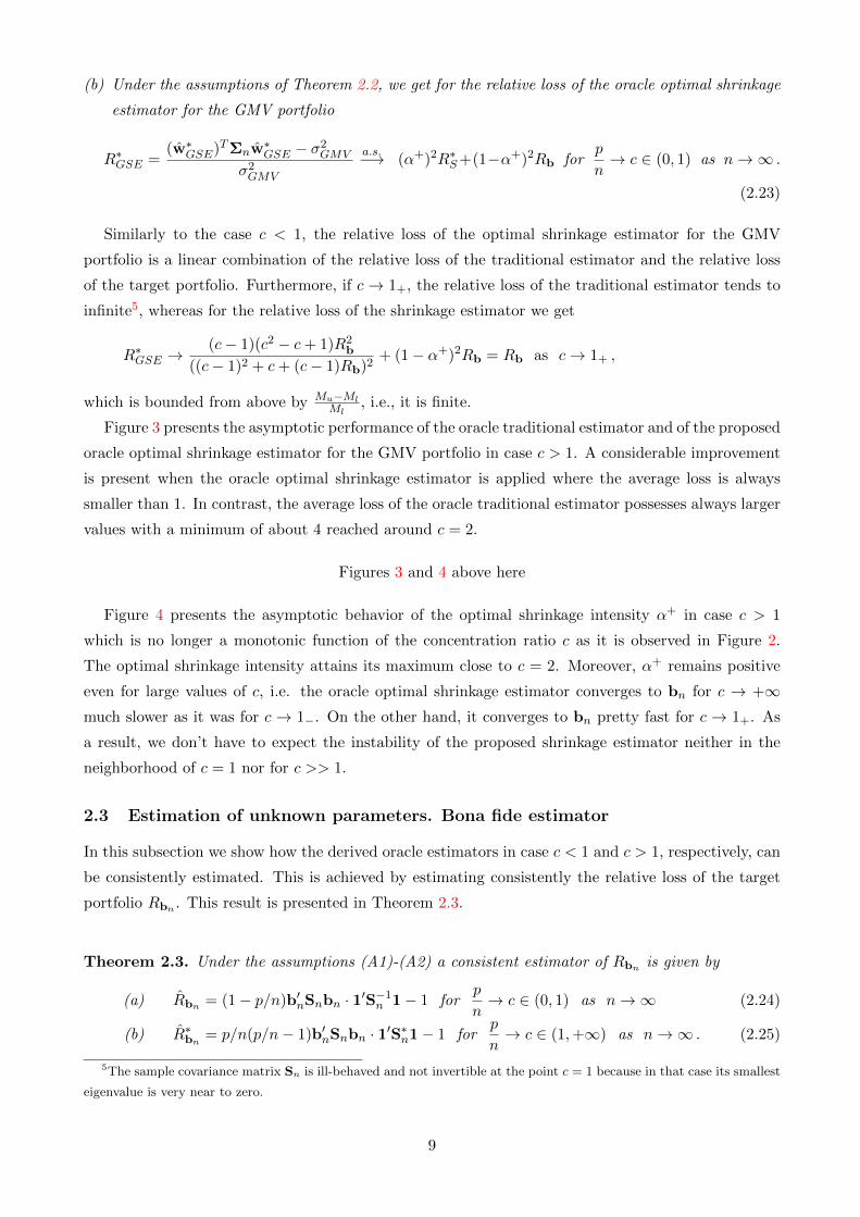
Figure 3 presents the asymptotic performance of the oracle traditional estimator and of the proposed

oracle optimal shrinkage estimator for the GMV portfolio in case c > 1. A considerable improvement

is present when the oracle optimal shrinkage estimator is applied where the average loss is always

smaller than 1. In contrast, the average loss of the oracle traditional estimator possesses always larger

values with a minimum of about 4 reached around c = 2.


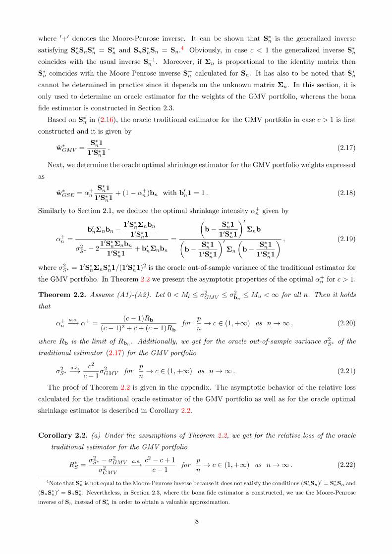
Figure 4 presents the asymptotic behavior of the optimal shrinkage intensity α+ in case c > 1

which is no longer a monotonic function of the concentration ratio c as it is observed in Figure 2.

The optimal shrinkage intensity attains its maximum close to c = 2. Moreover, α+ remains positive

even for large values of c, i.e. the oracle optimal shrinkage estimator converges to bn for c → +∞much slower as it was for c → 1−. On the other hand, it converges to bn pretty fast for c → 1+. As

a result, we don’t have to expect the instability of the proposed shrinkage estimator neither in the

neighborhood of c = 1 nor for c >> 1.

2.3 Estimation of unknown parameters. Bona fide estimator

In this subsection we show how the derived oracle estimators in case c < 1 and c > 1, respectively, can

be consistently estimated. This is achieved by estimating consistently the relative loss of the target

portfolio Rbn . This result is presented in Theorem 2.3.

Theorem 2.3. Under the assumptions (A1)-(A2) a consistent estimator of Rbn is given by

(a) Rbn = (1− p/n)b′nSnbn · 1′S−1n 1− 1 forp

n→ c ∈ (0, 1) as n→∞ (2.24)

(b) R∗bn= p/n(p/n− 1)b′nSnbn · 1′S∗n1− 1 for

p

n→ c ∈ (1,+∞) as n→∞ . (2.25)

5The sample covariance matrix Sn is ill-behaved and not invertible at the point c = 1 because in that case its smallest

eigenvalue is very near to zero.

9

The proof of Theorem 2.3 is given in the appendix. Applying Theorems 2.1 and 2.3(a) allows us

to determine the bona fide estimator for the GMV portfolio weights in case c ∈ (0, 1). It is given by

wBFGSE = α∗S−1n 1

1′S−1n 1+ (1− α∗)bn with α∗ =

(1− p/n)Rbn

p/n+ (1− p/n)Rbn

, (2.26)

where Rbn is given above in (2.24). The expression (2.26) presents the optimal shrinkage estimator

for a given target portfolio bn because the shrinkage intensity α∗ tends almost surely to its optimal

value α∗ for p/n→ c ∈ (0, 1) as n→∞.The situation is more complicated in case c > 1. Here, the quantity Rbn is not a bona fide estimator

of the relative loss of the target portfolio, since the matrix S∗n depends on unknown quantities. For

that reason we propose a reasonable approximation via the the application of the Moore-Penrose

inverse S+n . It is easy to verify that in case of Σn = σ2I equality holds. Furthermore, both the

extensive simulation study of Section 3 and the empirical investigations of Section 4 document that

this approximation does a very good job even for dense6 population covariance matrix Σn. The reason

of this behavior could be the point that S+n possesses a similar asymptotic behavior as S∗n. However,

it is a very challenging mathematical problem to prove this result analytically and we leave this for

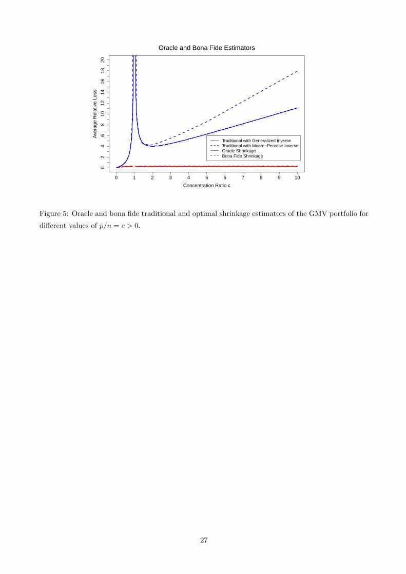
the future research. In Figure 6 we provide a short simulation with the same design as presented in

Figure 2 in order to show that α∗(S+n ) and α∗(S∗n) are close asymptotically and justify the accuracy

of our approximation.

Figures 6 above here

Taking into account the above discussion and the result of Theorem 2.3 (b), the bona fide estimator

of the quantity Rb in case c > 1 is approximated by

R+bn

= p/n(p/n− 1)b′nSnbn · 1′S+n 1− 1 for c ∈ (1,+∞) . (2.27)

The application of (2.27) leads to the bona fide optimal shrinkage estimator of the GMV portfolio in

case c > 1 expressed as

w+BFGSE = α+ S+

n 1

1′S+n 1

+ (1− α+)bn with α+ =(p/n− 1)R+

bn

(p/n− 1)2 + p/n+ (p/n− 1)R+bn

, (2.28)

where S+n is the Moore-Penrose pseudo-inverse of the sample covariance matrix Sn.

It is noted that the estimator (2.26) is the optimal estimator of the GMV portfolio for c < 1 in

terms of minimizing the out-of-sample variance, while the estimator (2.28) is a suboptimal one in case

c > 1. In order to summarize this section, we merge (2.26) and (2.28) into one bona fide optimal

shrinkage estimator for the GMV portfolio weights in case c > 0 given by7

wBFGSE = α∗S+n 1

1′S+n 1

+ (1− α∗)bn with (2.29)

6opposite of sparse.7The case c = 1 is not theoretically handled but using the Moore-Penrose inverse and setting equal to zero the smallest

eigenvalue we are still able to construct a feasible estimator in this situation.

10

α∗ =

(1− p/n)Rbn

p/n+ (1− p/n)Rbn

for c < 1,

(p/n− 1)Rbn

(p/n− 1)2 + p/n+ (p/n− 1)Rbn

for c ≥ 1 ,

(2.30)

and

Rbn =

{(1− p/n)b′nSnbn · 1′S−1n 1− 1 for c < 1,

p/n(p/n− 1)b′nSnbn · 1′S+n 1− 1 for c ≥ 1 .

, (2.31)

where we use that S+n = S−1n if Sn is nonsingular.

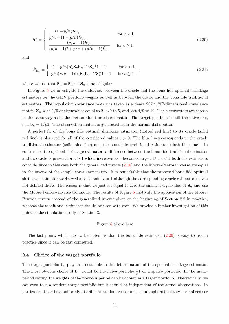
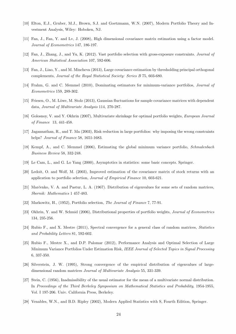
In Figure 5 we investigate the difference between the oracle and the bona fide optimal shrinkage

estimators for the GMV portfolio weights as well as between the oracle and the bona fide traditional

estimators. The population covariance matrix is taken as a dense 207 × 207-dimensional covariance

matrix Σn with 1/9 of eigenvalues equal to 2, 4/9 to 5, and last 4/9 to 10. The eigenvectors are chosen

in the same way as in the section about oracle estimator. The target portfolio is still the naive one,

i.e., bn = 1/p1. The observation matrix is generated from the normal distribution.

A perfect fit of the bona fide optimal shrinkage estimator (dotted red line) to its oracle (solid

red line) is observed for all of the considered values c > 0. The blue lines corresponds to the oracle

traditional estimator (solid blue line) and the bona fide traditional estimator (dash blue line). In

contrast to the optimal shrinkage estimator, a difference between the bona fide traditional estimator

and its oracle is present for c > 1 which increases as c becomes larger. For c < 1 both the estimators

coincide since in this case both the generalized inverse (2.16) and the Moore-Penrose inverse are equal

to the inverse of the sample covariance matrix. It is remarkable that the proposed bona fide optimal

shrinkage estimator works well also at point c = 1 although the corresponding oracle estimator is even

not defined there. The reason is that we just set equal to zero the smallest eigenvalue of Sn and use

the Moore-Penrose inverse technique. The results of Figure 5 motivate the application of the Moore-

Penrose inverse instead of the generalized inverse given at the beginning of Section 2.2 in practice,

whereas the traditional estimator should be used with care. We provide a further investigation of this

point in the simulation study of Section 3.

Figure 5 above here

The last point, which has to be noted, is that the bona fide estimator (2.29) is easy to use in

practice since it can be fast computed.

2.4 Choice of the target portfolio

The target portfolio bn plays a crucial role in the determination of the optimal shrinkage estimator.

The most obvious choice of bn would be the naive portfolio 1p1 or a sparse portfolio. In the multi-

period setting the weights of the previous period can be chosen as a target portfolio. Theoretically, we

can even take a random target portfolio but it should be independent of the actual observations. In

particular, it can be a uniformly distributed random vector on the unit sphere (suitably normalized) or

11

a uniformly distributed random vector on the simplex. Choosing the optimal portfolio weights of the

previous periods leads to more interesting example for a target portfolio which allows us to construct

some sort of Bayesian updating principle in the dynamic setting.

In general, the answer on this question depends on the underlying data because the choice of the

target weights is equivalent to the choice of the hyperparameter for the prior distribution of Σ−1n 1

1′Σ−1n 1

.

This problem is well-known in Bayesian statistics. The application of different priors leads to different

results. So it is very important to choose the one which works well in most cases. The naive one is

the equally weighted portfolio 1/p1. Obviously, the oracle shrinkage estimator with the prior weights

as the true global minimum variance portfolio is a consistent estimator as shown in Proposition 2.1.

Moreover, including some new information about the true GMV portfolio into the prior can lead to

a significant increase of performance (see, Bodnar et al. (2014)). For simplicity we take the naive

portfolio in our simulation study in Section 3 as well as in the empirical investigation of Section 4.

Consider the shinkage estimator as a vector function wBFGSE(bn) : Vp → Vp, where Vp and Vp

are the p-dimensional vector spaces. In the following proposition we present some properties of the

shrinkage estimator as a function of the target weights bn.

Proposition 2.1. For the proposed shrinkage estimator wBFGSE(bn) it holds that

1. wBFGSE(1/p1) is a consistent estimator for the GMV portfolio if the population covariance

matrix Σn = σI for arbitrary σ > 0 and c ∈ (0,+∞).

2. wBFGSE(wGMV ) is a consistent estimator for the GMV portfolio Σ−1n 1

1′Σ−1n 1

for all c ∈ (0,+∞).

The proof is a straightforward application of Theorem 2.1, Theorem 2.2 and Theorem 2.3.

3 Simulation study

In this section we demonstrate how the obtained results can be applied in practice. The first part of

our simulations is dedicated to normally distributed data, while in the second part the asset returns

are generated from the t-distribution with 5 degrees of freedom. The target portfolio bn is taken as

the naive portfolio1

p. The results are presented in both cases c < 1 and c > 1 as well as for the

covariance matrix with bounded (Section 3.1) and unbounded (Section 3.2) spectrum.

The benchmark estimator is the dominating estimator of the GMV portfolio suggested by Frahm

and Memmel (2010). It is given by

wFM = (1− k)S−1n 1′

1′S−1n 1+ k

1

pwith k =

p− 3

n− p+ 2

1

R1/p

, (3.1)

where R1/p =1/p21′Sn1− σ2Sn

σ2Sn

is the estimated relative loss of the naive portfolio. The dominating

estimator (3.1) is derived under the assumption that the asset returns are normally distributed and

it dominates over the traditional estimator in terms of the out-of-sample variance (cf. Frahm and

Memmel (2010)). Nevertheless, it is not clear how far it is away from the optimal one for different

values of the concentration ratio c > 0. Its behavior for non-normally distributed data has not been

studied yet as well.

12

Next, we compare the performance of the dominating estimator (3.1) with the bona fide optimal

shrinkage estimator (2.29). In order to find out the rates of convergence established in Theorem 2.1

and 2.3, we also consider the oracle optimal shrinkage estimator which can be easily constructed for

c < 1 and c > 1 with the optimal shrinkage intensities given by (2.10) and (2.19), respectively. As a

performance measure we take the relative loss from Section 2. For an arbitrary estimator w of the

GMV portfolio it is defined by

Rw =σ2w − σ2GMV

σ2GMV

(3.2)

where σ2w = w′Σnw and σ2GMV =1

1′Σ−1n 1.

In our simulation study we take p as a function of n. In particular, when n = 18·2j and p = 9·2j for

j ∈ [0, 5] the concentration ration c is always equal to 0.5 and p increases together with n exponentially.

That is why the small dimensions are presented with more points and the large ones with less. Similar

choices of p and n are also performed for other values of c ∈ {0.1, 0.9, 1.8}. Finally, it is noted that the

simulation results show a good convergent rate in terms of the relative loss for the bona fide optimal

shrinkage estimator to its oracle one already for p ≤ 100.

3.1 Population covariance matrix with bounded spectrum

In this subsection, we assume that the covariance matrix possesses a bounded spectrum, i.e. with

bounded maximum eigenvalue. Here, we use the structure of the covariance matrix as in Figure

5, i.e., we take 1/9 of its eigenvalues equal to 2, 4/9 equal to 5 and 4/9 equal to 10. The high-

dimensional covariance matrices constructed in this way possess uniformly the same spectral norm

and their eigenvalues are not very dispersed. Additionally, this choice of the covariance matrices

ensures that when the dimension p increases then the spectrum of the covariance matrices does not

change its behavior.


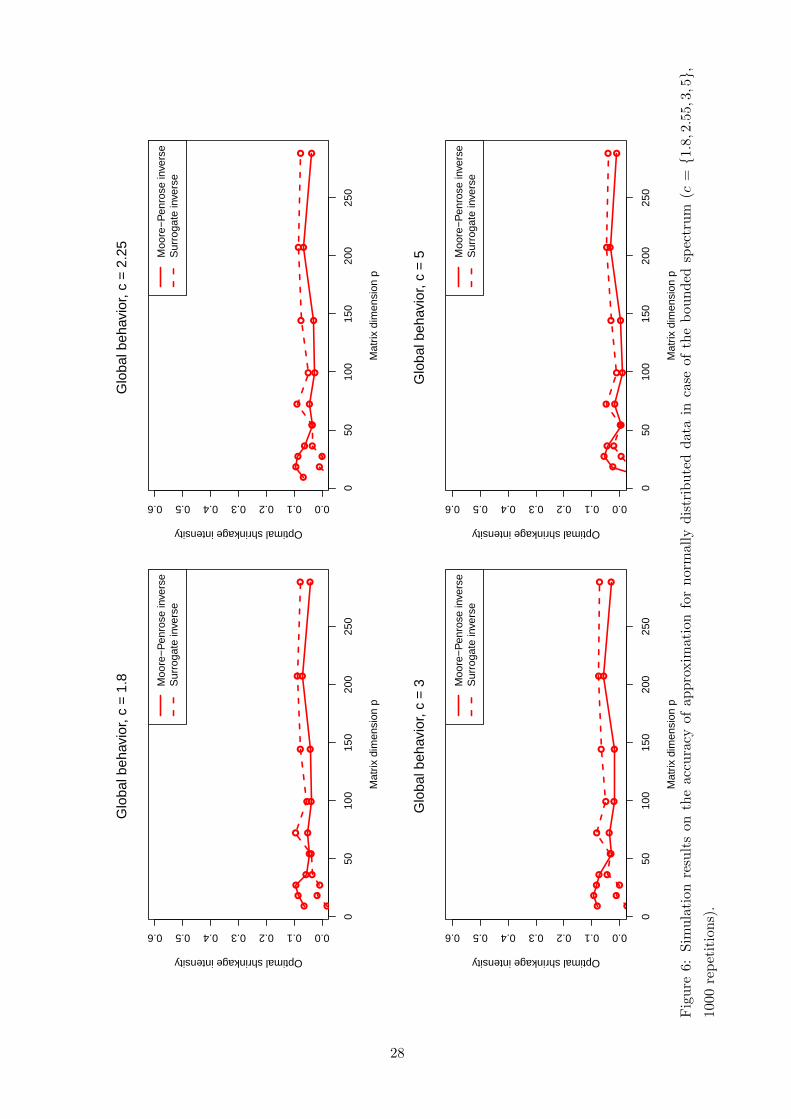
In Figures 7 and 8 we present the simulation results for normally distributed data and different

values of the concentration ratio c ∈ {0.1, 0.5, 0.9, 1.8}. Figure 7 presents the global behavior of

the considered estimators for different dimensions p, while Figure 8 shows the local distributional

properties for a value of fixed p = 306. More precisely, under the global behavior we understand the

evolution of the average relative loss with respect to the dimension p and the local behavior presents

the empirical cumulative distribution functions (e.c.d.f.) of the relative loss for one fixed value of p,

namely p = 306. The comparison in case of global setting is clear: the smaller the average loss the

better is the estimator. The local study provides a more precise comparison in terms of the empirical

distributions. In this case, the criterion of the best estimator is based on the observation that the

e.c.d.f. with stochastically smaller values is dominating. This means that for two e.c.d. functions, the

dominating one is placed on the left side from the other. This criterion is consistent with the stochastic

dominance of order one. The only difference with respect to the stochastic dominance of order one is

that the comparison is based on the empirical distribution functions instead of the population one.

13

On global analysis we see that the bona fide optimal shrinkage estimator converges to the corre-

sponding oracle one already for small values of p in all of the considered cases c ∈ {0.1, 0.5, 0.9, 1.8}.On the third place, the dominating estimator of Frahm and Memmel (2010) is ranked. It is always

better than the traditional estimator which is the worst one, but it is always worse than the other

two competitors. In terms of the values of the average relative loss, we observe that the difference

between the estimators become more significant if c increases and lies below 1.0. For instance, in

case of c = 0.1, the average relative loss of the traditional estimator tends to 1/9, whereas it tends

to 1 for c = 0.5. These two results are in line with Corollary 2.1, where it is proved that the average

loss of the traditional estimator tends to c/(1 − c) under high-dimensional asymptotics. In case of

c = 0.9, the difference between the average relative loss of the optimal shrinkage estimator and the

dominating (traditional) estimators becomes very large. Indeed, in this case the traditional estimator

has an average relative loss which is asymptotically equal to 9. This means that the out-of-sample risk

of the traditional estimator is 10 times larger than the real risk. The dominating estimator clearly

overperforms the traditional one but the relative loss is close to 4 for small dimensions (p ≤ 50) which

means that its out-of-sample risk is 5 times as large as the real risk. This is not acceptable anymore.

In contrast, the bona fide optimal shrinkage estimator converges fast to its oracle one. The relative

loss of the optimal shrinkage estimator is smaller than 0.3.

Figure 8 shows the same dominance in terms of the empirical distribution functions for a local

analysis in the case p = 306. The best approaches are the oracle and the bona fide optimal shrinkage

estimators. Next, the dominating estimator is ranked followed by the traditional one. The plots

also illustrate the fast convergence of the bona fide optimal shrinkage estimator to its oracle. The

local analysis for p = 306 confirms the almost sure convergence (consistence) of the bona fide optimal

shrinkage estimator which is proved in Theorem 2.1. In Figure 8 the relative risk of both the bona

fide and the oracle optimal shrinkage estimators possesses a very small variance which vanishes when

the dimension p increases. At the same time, the dominating estimator possesses a significantly larger

variance and it is unstable when c is close to one. The traditional estimator shows a very crucial

behavior and it is the worst one among the considered estimators.

The most interesting situation is observed for c = 1.8 in Figures 7 and 8 which corresponds to the

singular sample covariance matrix Sn. Here, we apply the results from Section 2.2 and 2.3 and take

the Moore-Penrose inverse S+n instead of S−1n . Note that we cannot use the dominating estimator

because it is not applicable for c > 1. The results are still impressing for both the global and the

local regimes. Again, the proposed bona fide optimal shrinkage estimator converges to its oracle. As

a traditional estimator, we take the GMV portfolio constructed by using the Moore-Penrose inverse

S+n . The traditional estimator possesses a rapidly increasing average loss and the largest variance. It

is not an acceptable estimator also for c > 1. In contrast, the bona fide optimal shrinkage estimator

has a small variance and obeys a stable behavior even if c > 1.

Further we analyze the behavior of the considered estimators when the asset returns are no longer

normally distributed. In particular it is interesting to study how strong is the impact of heavy tails

on the estimators derived in the paper. For this reason, the t-distribution with 5 degrees of freedom is

used next in our simulation study. Recently, authors have mentioned that 5 degrees of freedom seems

14

to be a suitable choice in practice (see, Venables and Ripley (2002)).


In Figures 9 and 10 we present the results for the t-distributed asset returns with 5 degrees of

freedom. The structure of the comparison study is the same as in case of normally distributed data.

In general, the behavior observed in Figures 9 and 10 does not differ significantly from those obtained

for the normal distribution. The best estimator is, as usual, the proposed shrinkage estimator. The

optimal shrinkage estimator dominates clearly other competitors over all c ∈ {0.1, 0.5, 0.9, 1.8}. It

is noted that the convergence rate of the bona fide optimal shrinkage estimator to its oracle is not

effected by the presence of heavy tails. A similar asymptotic relative loss behavior for the optimal

shrinkage estimator is established, i.e., the average relative loss is asymptotically constant and it is

smaller than 0.5. The traditional estimator possesses the worst behavior over all c and p.

3.2 Population covariance matrix with unbounded spectrum

In this subsection we assume that the largest eigenvalue of the population covariance matrix Σn

increases as O(p) when p→∞. Thus, the following structure of Σn is considered here, namely 1/9 of

eigenvalues equal to 2, 4/9 equal to 5, (4/9p− 1) equal to 10 and the last eigenvalue is equal to p.

Note that this structure corresponds to the case when a factor structure on the asset returns is

imposed. The factor model can reduce significantly the number of dimensions so that the estimators

do not suffer from the ”curse of dimensionality” anymore (see, e.g., Fan et al. (2013)).

Figures 11 to 14 above here

In Figures 11 to 14 we present the behavior of the estimators considered in the paper in case

of a covariance matrix with unbounded spectrum. It is remarkable to note that the results are not

very different from those obtained in case of a covariance matrix Σn with bounded spectrum. The

only difference is a somewhat greater variance of the estimators. On the other hand, the dominance

behavior as well as the convergence rate of the bona fide optimal shrinkage estimator to its oracle

is not effected by the largest eigenvalue of the population covariance matrix. This means that the

proposed estimator is still applicable if the asset returns follow a factor model. Even more, it does

not lose its efficiency also in case c > 1.

At the end, we note that, for the sake of interest, we have also simulated the t-distribution with

3 degrees of freedom for both the bounded and the unbounded spectra. This change effects only

the convergence rate but not the dominance behavior. In our theoretical framework we require the

existence of the 4th moment but the simulation study shows that this assumption can be relaxed or

conjectured to be relaxed. As a result, the proposed optimal shrinkage procedure assures the efficiency

in many important practical cases and, thus, can be applied in many real life situations. Nevertheless,

the empirical back-testing is still needed in order to check the behavior of the derived estimator for

the GMV portfolio weights on a real data set. This is done is the next section.

15

4 Empirical Study

In this section, we apply the proposed optimal shrinkage estimator for the GMV portfolio (2.29) to

real data which consist of daily returns on the 417 assets listed in the S&P 500 (Standard & Poor’s

500) index and traded during the period from 22.04.2013 to 19.03.2014. It corresponds to the horizon

of T = 230 trading days. The S&P 500 index is based on the market capitalizations of 500 large

companies having common stock listed on the NASDAQ.

In this empirical study we compare the performance of the derived optimal shrinkage estimator for

the GMV portfolio weights given by (2.29) with the traditional estimator and the dominating estimator

suggested by Frahm and Memmel (2010). The comparison is based a procedure which is similar to

the rolling-window approach proposed by DeMiguel et al. (2009). In particular, we randomly pick up

a portfolio of dimension p = 54 from all 417 portfolios and estimate the portfolio weights for the given

estimation window of the length n < T . We repeat this rolling-window procedure for the next step

by including data of the next day and dropping out the data of the last day until the end of the data

set is reached. The estimation window n is chosen such that the concentration ratio c = p/n lies in

the set {0.5, 0.9, 1.5, 2}.In order to compare the performance of the estimators we consider the out-of-sample variance and

the out-of-sample Sharpe ratio. Let wt be an estimator for the GMV portfolio which is based on the

window with last observation at time t and let rt+1 be the vector of the asset returns for the next

period t+ 1. Then the out-of-sample variance and the out-of-sample Sharpe ratio are calculated by

σ2out =1

T − n− 1

T−1∑t=n

(w′trt+1 − µt)2 and SR =µtσout

with µt =1

T − n

T−1∑t=n

w′trt+1 . (4.1)

In order to measure the statistical significance we sample randomly 1000 different portfolios and

calculate the e.c.d. functions of their out-of-sample variances and the corresponding out-of-sample

Sharpe ratios. The best strategy is chosen similarly to the stochastic dominance principle, i.e. we

look for the strategy whose e.c.d.f. stochastically dominates the other ones. However, the dominance

is defined differently in case of the out-of-sample variance and the out-of-sample Sharpe ratio. For

the out-of-sample variance, the e.c.d.f. of the best strategy should lie above the e.c.d. functions of

the other competitors, i.e. larger values of the out-of-sample variance can take place with smaller

probability. In contrast, criteria based on the out-of-sample Sharpe ratio prefers the strategy whose

e.c.d.f. lies below the other e.c.d. functions. In this case, the GMV portfolio constructed using the

corresponding estimator would possess the highest out-of-sample Sharpe ratio.


In Figures 15 and 16 the e.c.d. functions of the out-of-sample variance and of the out-of-sample

Sharpe ratio are presented for three estimators of the GMV portfolio, namely for the optimal shrinkage

estimator, the traditional estimator and the dominating estimator suggested by Frahm and Memmel

(2010). Because, the dominating estimator can be constructed only in case c < 1, we drop it for

c = 1.5 and c = 2. In all of the considered cases, we observe a very good performance of the optimal

shrinkage estimator. It overperforms the other estimation strategies for both considered criteria. The

16

corresponding e.c.d.f. lies above the other e.c.d. functions in case of the out-of-control variance,

whereas it is below the e.c.d. functions of other competitors in case of the out-of-sample Sharpe ratio.

On the second place, we rank the dominating estimator of Frahm and Memmel (2010) which is always

better than the traditional estimator.

5 Summary

The global minimum variance portfolio plays an important role in investment theory and practice.

This portfolio is widely used as an investment opportunity in both static and dynamic optimal portfolio

choice problems. Although an explicit analytical expression for the structure of the GMV portfolio

weights is available in literature, the estimation of the GMV portfolio appears to be a very challenging

problem, especially for high-dimensional data.

We deal with this problem in the present paper by deriving a feasible and robust estimator for

the weights of the GMV portfolio when the distribution of the asset returns is not prespecified and

no market structure is imposed. We construct an optimal shrinkage estimator for the GMV portfolio

which is optimal in the sense of minimizing the out-of-sample variance. An analytical expression

for the shrinkage intensity is obtained which appears to be a complicated function of the data and

the parameters of the asset return distribution. We deal with the later problem by determining an

asymptotically equivalent quantity of the shrinkage intensity under high-dimensional asymptotics. We

estimate this asymptotically equivalent function consistently by applying recent results from random

matrix theory. This is achieved under very weak assumptions imposed on the distribution of the asset

returns. Namely, we only require the existence of the fourth moment, whereas no explicit distributional

assumption is imposed. Moreover, our findings are still valid in both cases c < 1 and c > 1 as well

as if the spectrum of the population covariance matrix is bounded or unbounded. As a result, the

suggested method can be applied to heavy-tailed distributed asset returns as well as to asset returns

whose dynamics can be modeled by a factor model which is a very popular approach in financial

and econometric literature. Finally, using simulated and real data, we compare the optimal shrinkage

estimator for the GMV portfolio with existing ones. The theoretical findings as well as the results of

the Monte Carlo simulations and an empirical study show that the suggested estimator for the GMV

portfolio weights dominates the existing estimators in case c > 0.

6 Appendix

Here the proofs of the theorems are given. First, we point out that for our purposes Sn can be well

approximated by

Sn =1

nΣ

12nXn

(I− 1

n11′)

X′nΣ12n ≈

1

nΣ

12nXnX

′nΣ

12n ,

since the matrix1

n2Σ

12nXn11′X′nΣ

12n has rank one and, consequently, it does not influence the asymp-

totic behavior of the spectrum of the sample covariance matrix (see, Bai and Silverstein (2010),

Theorem A.44).

17

Next, we present an important lemma which is a special case of Theorem 1 in Rubio and Mestre

(2011).

Lemma 6.1. Assume (A1) and (A2). Let a nonrandom p × p-dimensional matrix Θp possess a

uniformly bounded trace norm (sum of singular values) and let Σn = I. Then it holds that∣∣tr (Θp(Sn − zIp)−1)− (x(z)− z)−1tr (Θp)

∣∣ a.s.−→ 0 for p/n −→ c ∈ (0,+∞) as n→∞ , (6.1)

where

x(z) =1

2

(1− c+ z +

√(1− c+ z)2 − 4z

). (6.2)

Proof of Lemma 6.1: The application of Theorem 1 in Rubio and Mestre (2011) leads to (6.1)

where x(z) is a unique solution in C+ of the following equation

1− x(z)

x(z)=

c

x(z)− z. (6.3)

The two solutions of (6.3) are given by

x1,2(z) =1

2

(1− c+ z ±

√(1− c+ z)2 − 4z

). (6.4)

In order to decide which of the two solutions is feasible, we note that x1,2(z) is the Stieltjes transform

with a positive imaginary part. Thus, without loss of generality, we can take z = 1 + c+ i2√c and get

Im{x1,2(z)} = Im

{1

2

(2 + i2

√c± i2

√2c)}

= Im{

1 + i√c(1±

√2)}

=√c(

1±√

2), (6.5)

which is positive only if the sign ” + ” is chosen. Hence, the solution is given by

x(z) =1

2

(1− c+ z +

√(1− c+ z)2 − 4z

). (6.6)

Lemma 6.1 is proved.

Rubio and Mestre (2011) studied the asymptotics of the functionals tr(Θ(Sn − zI)−1) for a deter-

ministic matrix Θ with bounded trace norm at infinity. Note that the results of Theorem 1 of Rubio

and Mestre (2011) also hold under the weaker assumption of the existence of the 4th moments. This

statement is obtained by using Lemma B.26 of Bai and Silverstein (2010) on quadratic forms which

we cite for presentation purposes as Lemma 6.2 below.

Lemma 6.2. [Lemma B.26, Bai and Silverstein (2010)] Let A be a p × p nonrandom matrix

and let X = (x1, . . . , xp)′ be a random vector with independent entries. Assume that E(xi) = 0,

E|xi|2 = 1, and E|xi|l ≤ νl. Then, for any k ≥ 1,

E|X′AX− tr(A)|k ≤ Ck(

(ν4tr(AA′))k2 + ν2ktr(AA′)

k2

), (6.7)

where Ck is some constant which depends only on k.

18

In order to obtain the statement of Theorem 1 of Rubio and Mestre (2011) under the weaker

assumption imposed on the moments, we replace Lemma 2 of Rubio and Mestre (2011) by Lemma 6.2

in the case of k ≥ 1. Note that Lemma 2 of Rubio and Mestre (2011) holds for k > 1 while Lemma 6.2

is a more stronger result because it holds also in the case k = 1. This is the main trick which implies

that Lemma 3 of Rubio and Mestre (2011) holds also for k ≥ 1 (instead of k > 1). Lemma 4 of Rubio

and Mestre (2011) has already been proved under the assumption that there exist 4 + ε moments.

The last step is the application of Lemma 1, 2 and 3 of Rubio and Mestre (2011) with k ≥ 1. Finally,

it can be easily checked that the further steps of the proof of Theorem 1 of Rubio and Mestre (2011)

hold under the existence of 4+ε moments. In order to save space we leave the detailed technical proof

of this assertion to the reader.

Proof of Theorem 2.1: Let us recall the optimal shrinkage intensity expressed as

α∗n =

b′nΣnbn −1′S−1n Σnbn

1′S−1n 11′S−1n ΣnS

−1n 1

(1′S−1n 1)2− 2

1′S−1n Σnbn

1′S−1n 1+ b′nΣnbn

. (6.8)

It holds that

1′S−1n 1 = limz→0+

tr[(Sn − zΣn)−111′

]= lim

z→0+tr

[(1

nXnX

′n − zI

)−1Σ− 1

2n 11′Σ

− 12

n

](6.9)

1′S−1n Σnbn = limz→0+

tr[(Sn − zΣn)−1Σnbn1

′]= lim

z→0+tr

[(1

nXnX

′n − zI

)−1Σ

12nbn1

′Σ− 1

2n

](6.10)

1′S−1n ΣnS−1n 1 =

∂

∂ztr

[(1

nSn − zΣn

)−111′

]∣∣∣∣∣z=0

=∂

∂ztr

[(1

nXnX

′n − zI

)−1Σ− 1

2n 11′Σ

− 12

n

]∣∣∣∣∣z=0

. (6.11)

Let

ξn(z) = tr

[(1

nXnX

′n − zI

)−1Θξ

]with Θξ = Σ

− 12

n 11′Σ− 1

2n

and

ζn(z) = tr

[(1

nXnX

′n − zI

)−1Θζ

]with Θζ = Σ

12nbn1

′Σ− 1

2n .

Both the matrices Θξ and Θζ possess a bounded trace norm since

‖Θξ‖tr = 1′Σ−1n 1 ≤M−1l

and

‖Θζ‖tr =

√1′Σ−1n 1

√b′nΣnbn ≤

√Mu

Ml.

19

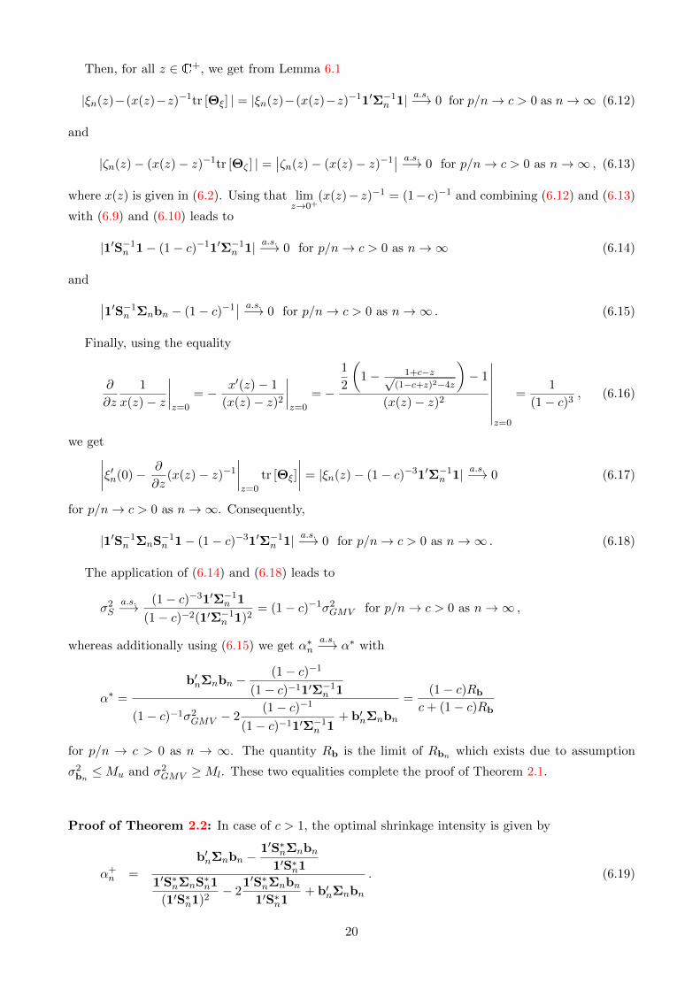
Then, for all z ∈ C+, we get from Lemma 6.1

|ξn(z)−(x(z)−z)−1tr [Θξ] | = |ξn(z)−(x(z)−z)−11′Σ−1n 1| a.s.−→ 0 for p/n→ c > 0 as n→∞ (6.12)

and

|ζn(z)− (x(z)− z)−1tr [Θζ ] | =∣∣ζn(z)− (x(z)− z)−1

∣∣ a.s.−→ 0 for p/n→ c > 0 as n→∞ , (6.13)

where x(z) is given in (6.2). Using that limz→0+

(x(z)− z)−1 = (1− c)−1 and combining (6.12) and (6.13)

with (6.9) and (6.10) leads to

|1′S−1n 1− (1− c)−11′Σ−1n 1| a.s.−→ 0 for p/n→ c > 0 as n→∞ (6.14)

and ∣∣1′S−1n Σnbn − (1− c)−1∣∣ a.s.−→ 0 for p/n→ c > 0 as n→∞ . (6.15)

Finally, using the equality

∂

∂z

1

x(z)− z

∣∣∣∣z=0

= − x′(z)− 1

(x(z)− z)2

∣∣∣∣z=0

= −

1

2

(1− 1+c−z√

(1−c+z)2−4z

)− 1

(x(z)− z)2

∣∣∣∣∣∣∣∣z=0

=1

(1− c)3, (6.16)

we get∣∣∣∣ξ′n(0)− ∂

∂z(x(z)− z)−1

∣∣∣∣z=0

tr [Θξ]

∣∣∣∣ = |ξn(z)− (1− c)−31′Σ−1n 1| a.s.−→ 0 (6.17)

for p/n→ c > 0 as n→∞. Consequently,

|1′S−1n ΣnS−1n 1− (1− c)−31′Σ−1n 1| a.s.−→ 0 for p/n→ c > 0 as n→∞ . (6.18)

The application of (6.14) and (6.18) leads to

σ2Sa.s.−→ (1− c)−31′Σ−1n 1

(1− c)−2(1′Σ−1n 1)2= (1− c)−1σ2GMV for p/n→ c > 0 as n→∞ ,

whereas additionally using (6.15) we get α∗na.s.−→ α∗ with

α∗ =

b′nΣnbn −(1− c)−1

(1− c)−11′Σ−1n 1

(1− c)−1σ2GMV − 2(1− c)−1

(1− c)−11′Σ−1n 1+ b′nΣnbn

=(1− c)Rb

c+ (1− c)Rb

for p/n → c > 0 as n → ∞. The quantity Rb is the limit of Rbn which exists due to assumption

σ2bn≤Mu and σ2GMV ≥Ml. These two equalities complete the proof of Theorem 2.1.

Proof of Theorem 2.2: In case of c > 1, the optimal shrinkage intensity is given by

α+n =

b′nΣnbn −1′S∗nΣnbn

1′S∗n1

1′S∗nΣnS∗n1

(1′S∗n1)2− 2

1′S∗nΣnbn1′S∗n1

+ b′nΣnbn

. (6.19)

20

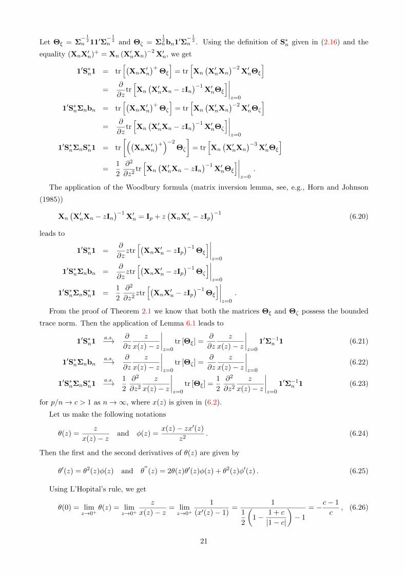
Let Θξ = Σ− 1

2n 11′Σ

− 12

n and Θζ = Σ12nbn1

′Σ− 1

2n . Using the definition of S∗n given in (2.16) and the

equality (XnX′n)+ = Xn (X′nXn)−2 X′n, we get

1′S∗n1 = tr[(

XnX′n

)+Θξ

]= tr

[Xn

(X′nXn

)−2X′nΘξ

]=

∂

∂ztr[Xn

(X′nXn − zIn

)−1X′nΘξ

]∣∣∣∣z=0

1′S∗nΣnbn = tr[(

XnX′n

)+Θζ

]= tr

[Xn

(X′nXn

)−2X′nΘζ

]=

∂

∂ztr[Xn

(X′nXn − zIn

)−1X′nΘζ

]∣∣∣∣z=0

1′S∗nΣnS∗n1 = tr

[((XnX

′n

)+)−2Θζ

]= tr

[Xn

(X′nXn

)−3X′nΘξ

]=

1

2

∂2

∂z2tr[Xn

(X′nXn − zIn

)−1X′nΘξ

]∣∣∣∣z=0

.

The application of the Woodbury formula (matrix inversion lemma, see, e.g., Horn and Johnson

(1985))

Xn

(X′nXn − zIn

)−1X′n = Ip + z

(XnX

′n − zIp

)−1(6.20)

leads to

1′S∗n1 =∂

∂zztr[(

XnX′n − zIp

)−1Θξ

]∣∣∣∣z=0

1′S∗nΣnbn =∂

∂zztr[(

XnX′n − zIp

)−1Θζ

]∣∣∣∣z=0

1′S∗nΣnS∗n1 =

1

2

∂2

∂z2ztr[(

XnX′n − zIp

)−1Θξ

]∣∣∣∣z=0

.

From the proof of Theorem 2.1 we know that both the matrices Θξ and Θζ possess the bounded

trace norm. Then the application of Lemma 6.1 leads to

1′S∗n1a.s.−→ ∂

∂z

z

x(z)− z

∣∣∣∣z=0

tr [Θξ] =∂

∂z

z

x(z)− z

∣∣∣∣z=0

1′Σ−1n 1 (6.21)

1′S∗nΣnbna.s.−→ ∂

∂z

z

x(z)− z

∣∣∣∣z=0

tr [Θζ ] =∂

∂z

z

x(z)− z

∣∣∣∣z=0

(6.22)

1′S∗nΣnS∗n1

a.s.−→ 1

2

∂2

∂z2z

x(z)− z

∣∣∣∣z=0

tr [Θξ] =1

2

∂2

∂z2z

x(z)− z

∣∣∣∣z=0

1′Σ−1n 1 (6.23)

for p/n→ c > 1 as n→∞, where x(z) is given in (6.2).

Let us make the following notations

θ(z) =z

x(z)− zand φ(z) =

x(z)− zx′(z)z2

. (6.24)

Then the first and the second derivatives of θ(z) are given by

θ′(z) = θ2(z)φ(z) and θ′′(z) = 2θ(z)θ′(z)φ(z) + θ2(z)φ′(z) . (6.25)

Using L’Hopital’s rule, we get

θ(0) = limz→0+

θ(z) = limz→0+

z

x(z)− z= lim

z→0+

1

(x′(z)− 1)=

1

1

2

(1− 1 + c

|1− c|

)− 1

= −c− 1

c, (6.26)

21

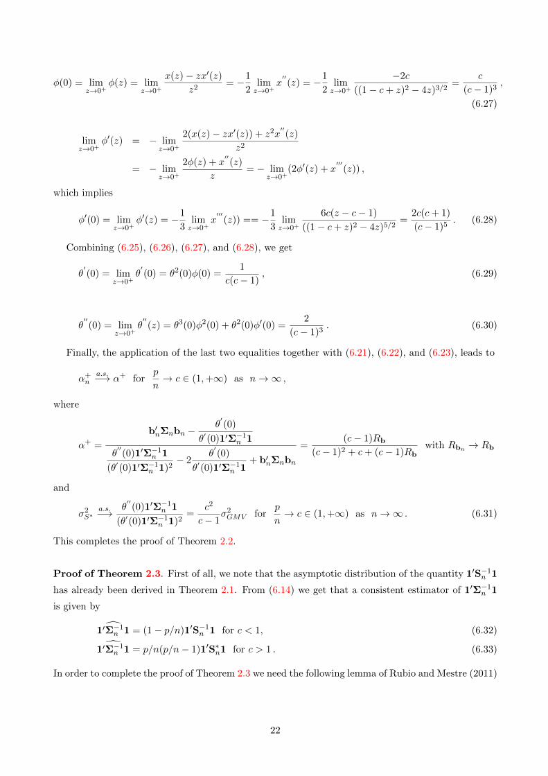
φ(0) = limz→0+

φ(z) = limz→0+

x(z)− zx′(z)z2

= −1

2limz→0+

x′′(z) = −1

2limz→0+

−2c

((1− c+ z)2 − 4z)3/2=

c

(c− 1)3,

(6.27)

limz→0+

φ′(z) = − limz→0+

2(x(z)− zx′(z)) + z2x′′(z)

z2

= − limz→0+

2φ(z) + x′′(z)

z= − lim

z→0+(2φ′(z) + x

′′′(z)) ,

which implies

φ′(0) = limz→0+

φ′(z) = −1

3limz→0+

x′′′

(z)) == −1

3limz→0+

6c(z − c− 1)

((1− c+ z)2 − 4z)5/2=

2c(c+ 1)

(c− 1)5. (6.28)

Combining (6.25), (6.26), (6.27), and (6.28), we get

θ′(0) = lim

z→0+θ′(0) = θ2(0)φ(0) =

1

c(c− 1), (6.29)

θ′′(0) = lim

z→0+θ′′(z) = θ3(0)φ2(0) + θ2(0)φ′(0) =

2

(c− 1)3. (6.30)

Finally, the application of the last two equalities together with (6.21), (6.22), and (6.23), leads to

α+n

a.s.−→ α+ forp

n→ c ∈ (1,+∞) as n→∞ ,

where

α+ =

b′nΣnbn −θ′(0)

θ′(0)1′Σ−1n 1

θ′′(0)1′Σ−1n 1

(θ′(0)1′Σ−1n 1)2− 2

θ′(0)

θ′(0)1′Σ−1n 1+ b′nΣnbn

=(c− 1)Rb

(c− 1)2 + c+ (c− 1)Rbwith Rbn → Rb

and

σ2S∗a.s.−→ θ

′′(0)1′Σ−1n 1

(θ′(0)1′Σ−1n 1)2=

c2

c− 1σ2GMV for

p

n→ c ∈ (1,+∞) as n→∞ . (6.31)

This completes the proof of Theorem 2.2.

Proof of Theorem 2.3. First of all, we note that the asymptotic distribution of the quantity 1′S−1n 1

has already been derived in Theorem 2.1. From (6.14) we get that a consistent estimator of 1′Σ−1n 1

is given by

1′Σ−1n 1 = (1− p/n)1′S−1n 1 for c < 1, (6.32)1′Σ−1n 1 = p/n(p/n− 1)1′S∗n1 for c > 1 . (6.33)

In order to complete the proof of Theorem 2.3 we need the following lemma of Rubio and Mestre (2011)

22

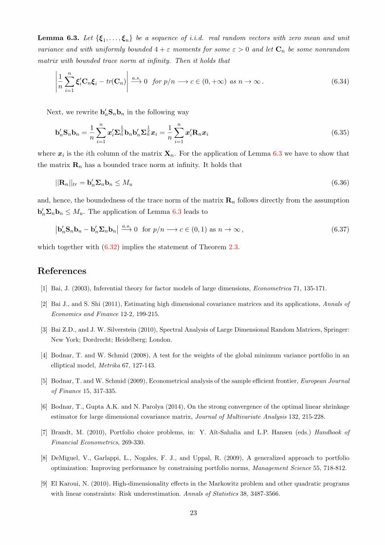
Lemma 6.3. Let {ξ1, . . . , ξn} be a sequence of i.i.d. real random vectors with zero mean and unit

variance and with uniformly bounded 4 + ε moments for some ε > 0 and let Cn be some nonrandom

matrix with bounded trace norm at infinity. Then it holds that∣∣∣∣∣ 1nn∑i=1

ξ′iCnξi − tr(Cn)

∣∣∣∣∣ a.s.−→ 0 for p/n −→ c ∈ (0,+∞) as n→∞ . (6.34)

Next, we rewrite b′nSnbn in the following way

b′nSnbn =1

n

n∑i=1

x′iΣ12nbnb

′nΣ

12nxi =

1

n

n∑i=1

x′iRnxi (6.35)

where xi is the ith column of the matrix Xn. For the application of Lemma 6.3 we have to show that

the matrix Rn has a bounded trace norm at infinity. It holds that

||Rn||tr = b′nΣnbn ≤Mu (6.36)

and, hence, the boundedness of the trace norm of the matrix Rn follows directly from the assumption

b′nΣnbn ≤Mu. The application of Lemma 6.3 leads to∣∣b′nSnbn − b′nΣnbn∣∣ a.s.−→ 0 for p/n −→ c ∈ (0, 1) as n→∞ , (6.37)

which together with (6.32) implies the statement of Theorem 2.3.

References

[1] Bai, J. (2003), Inferential theory for factor models of large dimensions, Econometrica 71, 135-171.

[2] Bai J., and S. Shi (2011), Estimating high dimensional covariance matrices and its applications, Annals of

Economics and Finance 12-2, 199-215.

[3] Bai Z.D., and J. W. Silverstein (2010), Spectral Analysis of Large Dimensional Random Matrices, Springer:

New York; Dordrecht; Heidelberg; London.

[4] Bodnar, T. and W. Schmid (2008), A test for the weights of the global minimum variance portfolio in an

elliptical model, Metrika 67, 127-143.

[5] Bodnar, T. and W. Schmid (2009), Econometrical analysis of the sample efficient frontier, European Journal

of Finance 15, 317-335.

[6] Bodnar, T., Gupta A.K. and N. Parolya (2014), On the strong convergence of the optimal linear shrinkage

estimator for large dimensional covariance matrix, Journal of Multivariate Analysis 132, 215-228.

[7] Brandt, M. (2010), Portfolio choice problems, in: Y. Aıt-Sahalia and L.P. Hansen (eds.) Handbook of

Financial Econometrics, 269-330.

[8] DeMiguel, V., Garlappi, L., Nogales, F. J., and Uppal, R. (2009), A generalized approach to portfolio

optimization: Improving performance by constraining portfolio norms, Management Science 55, 718-812.

[9] El Karoui, N. (2010). High-dimensionality effects in the Markowitz problem and other quadratic programs

with linear constraints: Risk underestimation. Annals of Statistics 38, 3487-3566.

23

[10] Elton, E.J., Gruber, M.J., Brown, S.J. and Goetzmann, W.N. (2007), Modern Portfolio Theory and In-

vestment Analysis, Wiley: Hoboken, NJ.

[11] Fan, J., Fan, Y. and Lv, J. (2008), High dimensional covariance matrix estimation using a factor model.

Journal of Econometrics 147, 186-197.

[12] Fan, J., Zhang, J., and Yu, K. (2012). Vast portfolio selection with gross-exposure constraints. Journal of

American Statistical Association 107, 592-606.

[13] Fan, J., Liao, Y., and M. Mincheva (2013), Large covariance estimation by thresholding principal orthogonal

complements, Journal of the Royal Statistical Society: Series B 75, 603-680.

[14] Frahm, G. and C. Memmel (2010), Dominating estimators for minimum-variance portfolios, Journal of

Econometrics 159, 289-302.

[15] Friesen, O., M. Lowe, M. Stolz (2013), Gaussian fluctuations for sample covariance matrices with dependent

data, Journal of Multivariate Analysis 114, 270-287.

[16] Golosnoy, V. and Y. Okhrin (2007), Multivariate shrinkage for optimal portfolio weights, European Journal

of Finance 13, 441-458.

[17] Jagannathan, R., and T. Ma (2003), Risk reduction in large portfolios: why imposing the wrong constraints

helps? Journal of Finance 58, 1651-1683.

[18] Kempf, A., and C. Memmel (2006), Estimating the global minimum variance portfolio, Schmalenbach

Business Review 58, 332-248.

[19] Le Cam, L., and G. Lo Yang (2000), Asymptotics in statistics: some basic concepts. Springer.

[20] Ledoit, O. and Wolf, M. (2003), Improved estimation of the covariance matrix of stock returns with an

application to portfolio selection, Journal of Empirical Finance 10, 603-621.

[21] Marcenko, V. A. and Pastur, L. A. (1967). Distribution of eigenvalues for some sets of random matrices,

Sbornik: Mathematics 1 457-483.

[22] Markowitz, H., (1952), Portfolio selection, The Journal of Finance 7, 77-91.

[23] Okhrin, Y. and W. Schmid (2006), Distributional properties of portfolio weights, Journal of Econometrics

134, 235-256.

[24] Rubio F., and X. Mestre (2011), Spectral convergence for a general class of random matrices, Statistics

and Probability Letters 81, 592-602.

[25] Rubio F., Mestre X., and D.P. Palomar (2012), Performance Analysis and Optimal Selection of Large

Minimum Variance Portfolios Under Estimation Risk, IEEE Journal of Selected Topics in Signal Processing

6, 337-350.

[26] Silverstein, J. W. (1995), Strong convergence of the empirical distribution of eigenvalues of large-

dimensional random matrices Journal of Multivariate Analysis 55, 331-339.

[27] Stein, C. (1956), Inadmissibility of the usual estimator for the mean of a multivariate normal distribution.

In Proceedings of the Third Berkeley Symposium on Mathematical Statistics and Probability, 1954-1955,

Vol. I 197-206. Univ. California Press, Berkeley.

[28] Venables, W.N., and B.D. Ripley (2002), Modern Applied Statistics with S, Fourth Edition, Springer.

24

Asymptotic behavior of the sample and optimal shrinkage estimators

Concentration Ratio c

Ave

rage

Rel

ativ

e Lo

ss

0.0 0.1 0.2 0.3 0.4 0.5 0.6 0.7 0.8 0.9 1.0

01

23

45

67

89

10 TraditionalOracle Shrinkage

Figure 1: Asymptotic relative loss of the traditional and the oracle shrinkage estimators as a function

of the concentration ratio p/n = c < 1.

0.0 0.2 0.4 0.6 0.8 1.0

0.0

0.2

0.4

0.6

0.8

1.0

Asymptotic behavior of the optimal shrinkage intensity


α

Figure 2: Asymptotic behavior of the optimal shrinkage intensity α∗ as a function of the concentration

ratio p/n = c < 1.

25

Asymptotic behavior of the sample and optimal shrinkage estimators


Ave

rage

Rel

ativ

e Lo

ss

1 2 3 4 5 6 7 8 9 10

02

46

810

1214

1618

20 Traditional with Generalized InverseOracle Shrinkage

Figure 3: Asymptotic relative loss of the oracle traditional estimator with generalized inverse (2.18)

and of the oracle optimal shrinkage estimator as a function of the concentration ratio p/n = c > 1.

0.0

0.1

0.2

0.3

0.4

0.5

Asymptotic behavior of the optimal shrinkage intensity


α

1 2 3 4 5 6 7 8 9 10

Figure 4: Asymptotic behavior of the optimal shrinkage intensity α+ as a function of the concentration

ratio p/n = c > 1.

26

Oracle and Bona Fide Estimators


Ave

rage

Rel

ativ

e Lo

ss

0 1 2 3 4 5 6 7 8 9 10

02

46

810

1214

1618

20

Traditional with Generalized InverseTraditional with Moore−Penrose InverseOracle ShrinkageBona Fide Shrinkage

Figure 5: Oracle and bona fide traditional and optimal shrinkage estimators of the GMV portfolio for

different values of p/n = c > 0.

27

●●

●

●●

●●

●●

●

050

100

150

200

250

0.00.10.20.30.40.50.6

Glo

bal b

ehav

ior,

c =

1.8

Mat

rix d

imen

sion

p

Optimal shrinkage intensity

●

●●

●●

●

●●

●●

Moo

re−

Pen

rose

inve

rse

Sur

roga

te in

vers

e

●●

●●

●●

●●

●

●

050

100

150

200

250

0.00.10.20.30.40.50.6

Glo

bal b

ehav

ior,

c =

2.2

5

Mat

rix d

imen

sion

p


●

●●

●●

●

●●

●●

Moo

re−

Pen

rose

inve

rse

Sur

roga

te in

vers

e

●●

●●

●●

●●

●●

050

100

150

200

250

0.00.10.20.30.40.50.6

Glo

bal b

ehav

ior,

c =

3

Mat

rix d

imen

sion

p


●

●●

●●

●

●●

●●

Moo

re−

Pen

rose

inve

rse

Sur

roga

te in

vers

e

●

●

●●

●●

●●

●●

050

100

150

200

250

0.00.10.20.30.40.50.6

Glo

bal b

ehav

ior,

c =

5

Mat

rix d

imen

sion

p


●

●

●●

●

●

●●

●●

Moo

re−

Pen

rose

inve

rse

Sur

roga

te in

vers

e

Fig

ure

6:S

imu

lati

onre

sult

son

the

accu

racy

ofap

pro

xim

atio

nfo

rn

orm

ally

dis

trib

ute

dd

ata

inca

seof

the

boun

ded

spec

tru

m(c

={1.8,2.5

5,3,

5},

1000

rep

etit

ion

s).

28

●●

●●

●●

●●

●●

050

100

150

200

250

0.00.20.40.60.81.0

Glo

bal b

ehav

ior,

c =

0.1

Mat

rix d

imen

sion

p

Average Relative Loss

●●

●●

●●

●●

●●

●●

●●

●●

●●

●●

●●

●●

●●

●●

●●

Trad

ition

alB

ona

Fid

e S

hrin

kage

Dom

inat

ing

Ora

cle

Shr

inka

ge

●●

●●

●●

●●

●●

050

100

150

200

250

0.00.51.01.52.0

Glo

bal b

ehav

ior,

c =

0.5

Mat

rix d

imen

sion

p


●●

●●

●●

●●

●●

●

●●

●●

●●

●●

●

●●

●●

●●

●●

●●

Trad

ition

alB

ona

Fid

e S

hrin

kage

Dom

inat

ing

Ora

cle

Shr

inka

ge

●●

●●

●●

●●

●●

050

100

150

200

250

0246810

Glo

bal b

ehav

ior,

c =

0.9

Mat

rix d

imen

sion

p


●●

●●

●●

●●

●●

●

●●

●

●●

●●

●●

●●

●●

●●

●●

●●

Trad

ition

alB

ona

Fid

e S

hrin

kage

Dom

inat

ing

Ora

cle

Shr

inka

ge

●●

●●

●

●●

●●

●

050

100

150

200

250

0246810

Glo

bal b

ehav

ior,

c =

1.8

Mat

rix d

imen

sion

p


●●

●●

●●

●●

●●

●●

●●

●●

●●

●●

Trad

ition

alB

ona

Fid

e S

hrin

kage

Ora

cle

Shr

inka

ge

Fig

ure

7:S

imu

lati

onre

sult

sfo

rn

orm

ally

dis

trib

ute

dd

ata

inca

seof

the

bou

nd

edsp

ectr

um

(c={0.1,0.5,0.9,1.8},

1000

rep

etit

ion

s).

29

0.0

0.2

0.4

0.6

0.8

1.0

0.00.20.40.60.81.0

Em

piric

al D

istr

ibut

ion

Fun

ctio

ns fo

r p=

306,

c=

0.1

Rel

ativ

e Lo

ss

Empirical Cumulative Distribution Function

Trad

ition

alB

ona

Fid

e S

hrin

kage

Ora

cle

Shr

inka

geD

omin

atin

g

0.0

0.5

1.0

1.5

2.0

0.00.20.40.60.81.0

Em

piric

al D

istr

ibut

ion

Fun

ctio

ns fo

r p=

306,

c=

0.5

Rel

ativ

e Lo

ss


Trad

ition

alB

ona

Fid

e S

hrin

kage

Ora

cle

Shr

inka

geD

omin

atin

g

02

46

810

1214

0.00.20.40.60.81.0

Em

piric

al D

istr

ibut

ion

Fun

ctio

ns fo

r p=

306,

c=

0.9

Rel

ativ

e Lo

ss


Trad

ition

alB

ona

Fid

e S

hrin

kage

Ora

cle

Shr

inka

geD

omin

atin

g

02

46

810

0.00.20.40.60.81.0

Em

piric

al D

istr

ibut

ion

Fun

ctio

ns fo

r p=

306,

c=

1.8

Rel

ativ

e Lo

ss

Empirical Cumulative Distribution FunctionTr

aditi

onal

Bon

a F

ide

Shr

inka

geO

racl

e S

hrin

kage

Fig

ure

8:S

imu

lati

onre

sult

sfo

rn

orm

ally

dis

trib

ute

dd

ata

inca

seof

the

bou

nd

edsp

ectr

um

(c={0.1,0.5,0.9,1.8},

1000

rep

etit

ion

s).

30

●●

●●

●●

●●

●●

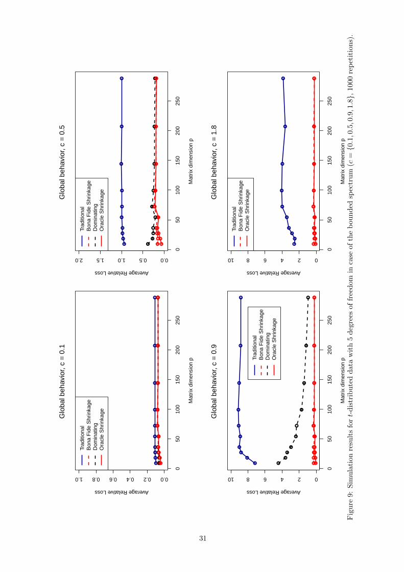
050

100

150

200

250

0.00.20.40.60.81.0

Glo

bal b

ehav

ior,

c =

0.1

Mat

rix d

imen

sion

p


●●

●●

●●

●●

●●

●●

●●

●●

●●

●●

●●

●●

●●

●●

●●

Trad

ition

alB

ona

Fid

e S

hrin

kage

Dom

inat

ing

Ora

cle

Shr

inka

ge

●●

●●

●●

●●

●●

050

100

150

200

250

0.00.51.01.52.0

Glo

bal b

ehav

ior,

c =

0.5

Mat

rix d

imen

sion

p


●●

●●

●●

●●

●●

●

●●

●●

●●

●●

●

●●

●●

●●

●●

●●

Trad

ition

alB

ona

Fid

e S

hrin

kage

Dom

inat

ing

Ora

cle

Shr

inka

ge

●

●

●●

●●

●●

●●

050

100

150

200

250

0246810

Glo

bal b

ehav

ior,

c =

0.9

Mat

rix d

imen

sion

p


●●

●●

●●

●●

●●

●

●●

●

●●

●●

●●

●●

●●

●●

●●

●●

Trad

ition

alB

ona

Fid

e S

hrin

kage

Dom

inat

ing

Ora

cle

Shr

inka

ge

●●

●●

●

●●

●●

●

050

100

150

200

250

0246810

Glo

bal b

ehav

ior,

c =

1.8

Mat

rix d

imen

sion

p


●●

●●

●●

●●

●●

●●

●●

●●

●●

●●

Trad

ition

alB

ona

Fid

e S

hrin

kage

Ora

cle

Shr

inka

ge

Fig

ure

9:S

imu

lati

onre

sult

sfo

rt-

dis

trib

ute

dd

ata

wit

h5

deg

rees

offr

eed

omin

case

ofth

eb

oun

ded

spec

tru

m(c

={0.1,0.5,0.9,1.8},

1000

rep

etit

ion

s).

31

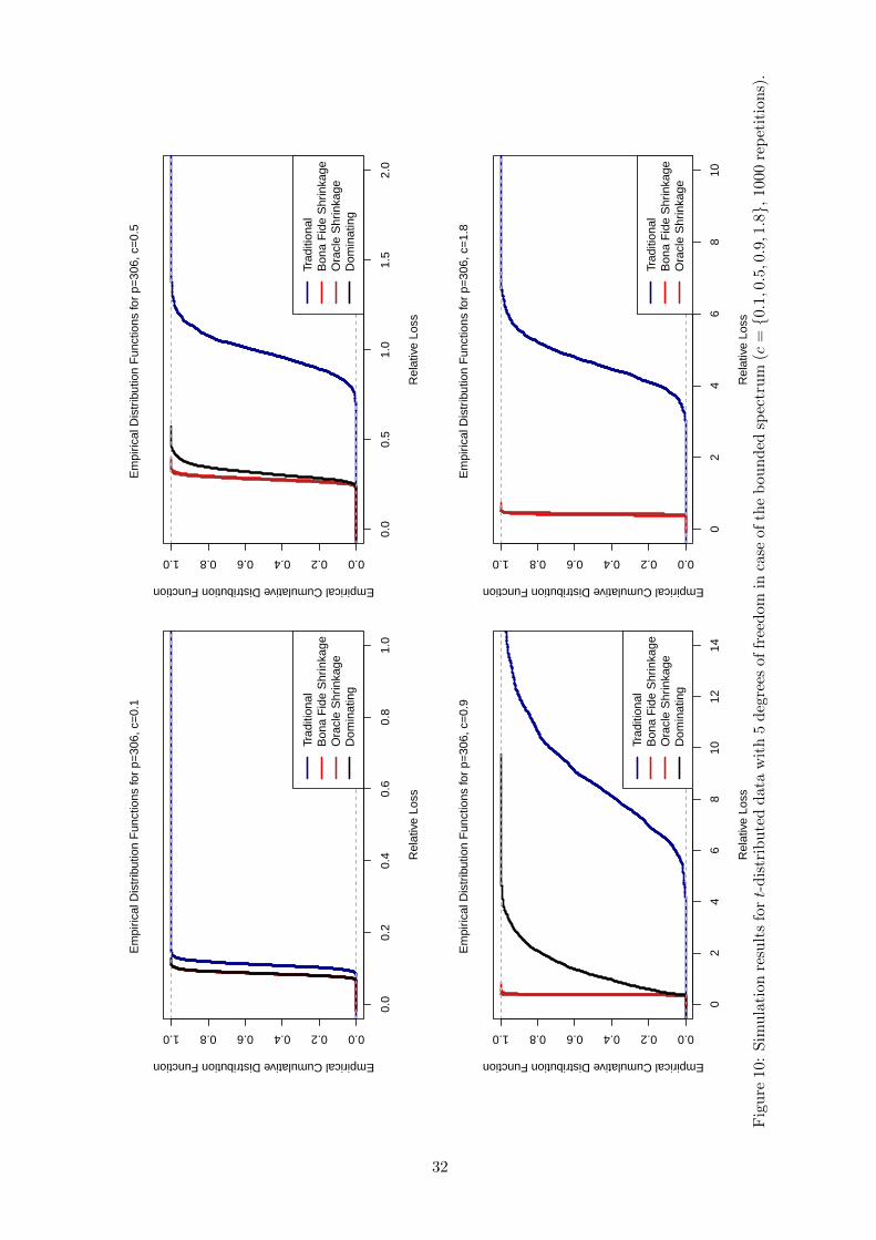
0.0

0.2

0.4

0.6

0.8

1.0

0.00.20.40.60.81.0

Em

piric

al D

istr

ibut

ion

Fun

ctio

ns fo

r p=

306,

c=

0.1

Rel

ativ

e Lo

ss


Trad

ition

alB

ona

Fid

e S

hrin

kage

Ora

cle

Shr

inka

geD

omin

atin

g

0.0

0.5

1.0

1.5

2.0

0.00.20.40.60.81.0

Em

piric

al D

istr

ibut

ion

Fun

ctio

ns fo

r p=

306,

c=

0.5

Rel

ativ

e Lo

ss


Trad

ition

alB

ona

Fid

e S

hrin

kage

Ora

cle

Shr

inka

geD

omin

atin

g

02

46

810

1214

0.00.20.40.60.81.0

Em

piric

al D

istr

ibut

ion

Fun

ctio

ns fo

r p=

306,

c=

0.9

Rel

ativ

e Lo

ss


Trad

ition

alB

ona

Fid

e S

hrin

kage

Ora

cle

Shr

inka

geD

omin

atin

g

02

46

810

0.00.20.40.60.81.0

Em

piric

al D

istr

ibut

ion

Fun

ctio

ns fo

r p=

306,

c=

1.8

Rel

ativ

e Lo

ss


aditi

onal

Bon

a F

ide

Shr

inka

geO

racl

e S

hrin

kage

Fig

ure

10:

Sim

ula

tion

resu

lts

fort-

dis

trib

ute

dd

ata

wit

h5

deg

rees

offr

eed

omin

case

ofth

eb

oun

ded

spec

tru

m(c

={0.1,0.5,0.9,1.8},

1000

rep

etit

ion

s).

32

●●

●●

●●

●●

●●

050

100

150

200

250

0.00.20.40.60.81.0

Glo

bal b

ehav

ior,

c =

0.1

Mat

rix d

imen

sion

p


●●

●●

●●

●●

●●

●●

●●

●●

●●

●●

●●

●●

●●

●●

●●

Trad

ition

alB

ona

Fid

e S

hrin

kage

Dom

inat

ing

Ora

cle

Shr

inka

ge

●●

●●

●●

●●

●●

050

100

150

200

250

0.00.51.01.52.0

Glo

bal b

ehav

ior,

c =

0.5

Mat

rix d

imen

sion

p


●●

●●

●●

●●

●●

●

●●

●●

●●

●●

●

●●

●●

●●

●●

●●

Trad

ition

alB

ona

Fid

e S

hrin

kage

Dom

inat

ing

Ora

cle

Shr

inka

ge

●

●●

●●

●●

●●

●

050

100

150

200

250

0246810

Glo

bal b

ehav

ior,

c =

0.9

Mat

rix d

imen

sion

p


●●

●●

●●

●●

●●

●

●●

●

●●

●●

●●

●●

●●

●●

●●

●●

Trad

ition

alB

ona

Fid

e S

hrin

kage

Dom

inat

ing

Ora

cle

Shr

inka

ge

●●

●●

●

●●

●●

●

050

100

150

200

250

0246810

Glo

bal b

ehav

ior,

c =

1.8

Mat

rix d

imen

sion

p


●●

●●

●●

●●

●●

●●

●●

●●

●●

●●

Trad

ition

alB

ona

Fid

e S

hrin

kage

Ora

cle

Shr

inka

ge

Fig

ure

11:

Sim

ula

tion

resu

lts

for

nor

mal

lyd

istr

ibu

ted

dat

ain

case

ofth

eu

nb

oun

ded

spec

tru

m(c

={0.1,0.5,0.9,1.8},

1000

rep

etit

ion

s).

33

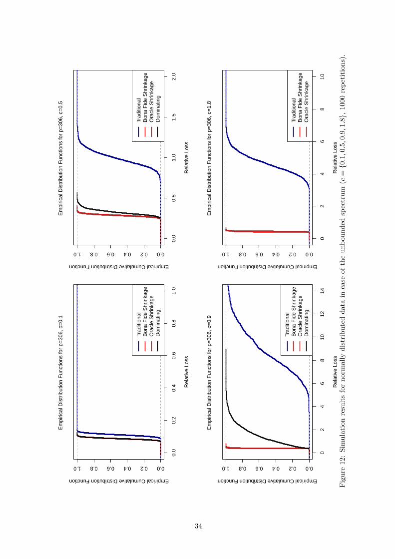
0.0

0.2

0.4

0.6

0.8

1.0

0.00.20.40.60.81.0

Em

piric

al D

istr

ibut

ion

Fun

ctio

ns fo

r p=

306,

c=

0.1

Rel

ativ

e Lo

ss


Trad

ition

alB

ona

Fid

e S

hrin

kage

Ora

cle

Shr

inka

geD

omin

atin

g

0.0

0.5

1.0

1.5

2.0

0.00.20.40.60.81.0

Em

piric

al D

istr

ibut

ion

Fun

ctio

ns fo

r p=

306,

c=

0.5

Rel

ativ

e Lo

ss


Trad

ition

alB

ona

Fid

e S

hrin

kage

Ora

cle

Shr

inka

geD

omin

atin

g

02

46

810

1214

0.00.20.40.60.81.0

Em

piric

al D

istr

ibut

ion

Fun

ctio

ns fo

r p=

306,

c=

0.9

Rel

ativ

e Lo

ss


Trad

ition

alB

ona

Fid

e S

hrin

kage

Ora

cle

Shr

inka

geD

omin

atin

g

02

46

810

0.00.20.40.60.81.0

Em

piric

al D

istr

ibut

ion

Fun

ctio

ns fo

r p=

306,

c=

1.8

Rel

ativ

e Lo

ss


aditi

onal

Bon

a F

ide

Shr

inka

geO

racl

e S

hrin

kage

Fig

ure

12:

Sim

ula

tion

resu

lts

for

nor

mal

lyd

istr

ibu

ted

dat

ain

case

ofth

eu

nb

oun

ded

spec

tru

m(c

={0.1,0.5,0.9,1.8},

1000

rep

etit

ion

s).

34

●●

●●

●●

●●

●●

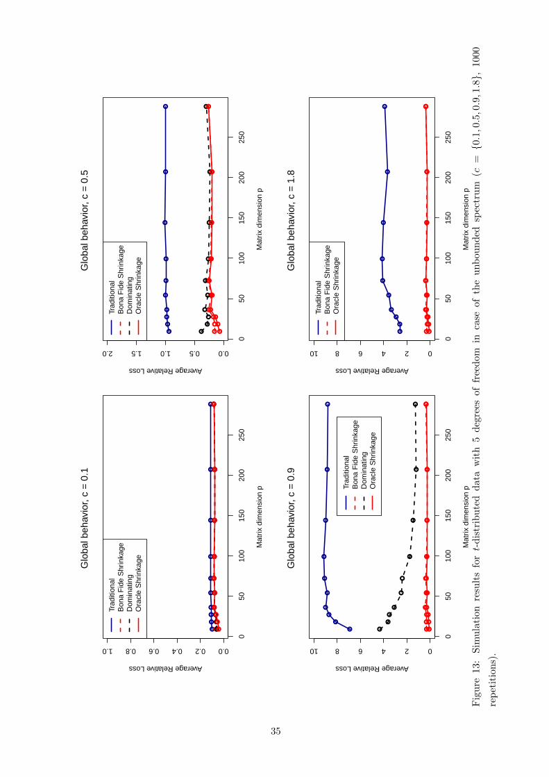
050

100

150

200

250

0.00.20.40.60.81.0

Glo

bal b

ehav

ior,

c =

0.1

Mat

rix d

imen

sion

p


●●

●●

●●

●●

●●

●●

●●

●●

●●

●●

●●

●●

●●

●●

●●

Trad

ition

alB

ona

Fid

e S

hrin

kage

Dom

inat

ing

Ora

cle

Shr

inka

ge

●●

●●

●●

●●

●●

050

100

150

200

250

0.00.51.01.52.0

Glo

bal b

ehav

ior,

c =

0.5

Mat

rix d

imen

sion

p


●●

●●

●●

●●

●●

●

●●

●●

●●

●●

●

●●

●●

●●

●●

●●

Trad

ition

alB

ona

Fid

e S

hrin

kage

Dom

inat

ing

Ora

cle

Shr

inka

ge

●

●

●●

●●

●●

●●

050

100

150

200

250

0246810

Glo

bal b

ehav

ior,

c =

0.9

Mat

rix d

imen

sion

p


●●

●●

●●

●●

●●

●

●●

●

●●

●●

●●

●●

●●

●●

●●

●●

Trad

ition

alB

ona

Fid

e S

hrin

kage

Dom

inat

ing

Ora

cle

Shr

inka

ge

●●

●●

●

●●

●●

●

050

100

150

200

250

0246810

Glo

bal b

ehav

ior,

c =

1.8

Mat

rix d

imen

sion

p


●●

●●

●●

●●

●●

●●

●●

●●

●●

●●

Trad

ition

alB

ona

Fid

e S

hrin

kage

Ora

cle

Shr

inka

ge

Fig

ure

13:

Sim

ula

tion

resu

lts

fort-

dis

trib

ute

dd

ata

wit

h5

deg

rees

offr

eed

omin

case

ofth

eu

nb

ou

nd

edsp

ectr

um

(c={0.1,0.5,0.9,1.8},

1000

rep

etit

ion

s).

35

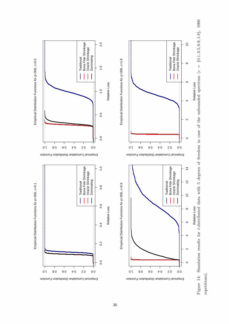
0.0

0.2

0.4

0.6

0.8

1.0

0.00.20.40.60.81.0

Em

piric

al D

istr

ibut

ion

Fun

ctio

ns fo

r p=

306,

c=

0.1

Rel

ativ

e Lo

ss


Trad

ition

alB

ona

Fid

e S

hrin

kage

Ora

cle

Shr

inka

geD

omin

atin

g

0.0

0.5

1.0

1.5

2.0

0.00.20.40.60.81.0

Em

piric

al D

istr

ibut

ion

Fun

ctio

ns fo

r p=

306,

c=

0.5

Rel

ativ

e Lo

ss


Trad

ition

alB

ona

Fid

e S

hrin

kage

Ora

cle

Shr

inka

geD

omin

atin

g

02

46

810

1214

0.00.20.40.60.81.0

Em

piric

al D

istr

ibut

ion

Fun

ctio

ns fo

r p=

306,

c=

0.9

Rel

ativ

e Lo

ss


Trad

ition

alB

ona

Fid

e S

hrin

kage

Ora

cle

Shr

inka

geD

omin

atin

g

02

46

810

0.00.20.40.60.81.0

Em

piric

al D

istr

ibut

ion

Fun

ctio

ns fo

r p=

306,

c=

1.8

Rel

ativ

e Lo

ss


aditi

onal

Bon

a F

ide

Shr

inka

geO

racl

e S

hrin

kage

Fig

ure

14:

Sim

ula

tion

resu

lts

fort-

dis

trib

ute

dd

ata

wit

h5

deg

rees

offr

eed

omin

case

ofth

eu

nb

ou

nd

edsp

ectr

um

(c={0.1,0.5,0.9,1.8},

1000

rep

etit

ion

s).

36

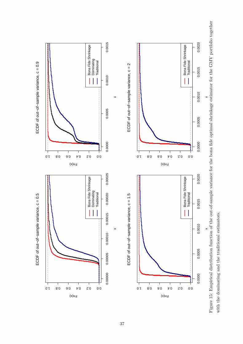
0.00

000

0.00

005

0.00

010

0.00

015

0.00

020

0.00

025

0.00.20.40.60.81.0

EC

DF

of o

ut−

of−

sam

ple

varia

nce,

c =

0.5

x

Fn(x)

Bon

a F

ide

Shr

inka

geD

omin

atin

gTr

aditi

onal

0.00

000.

0005

0.00

100.

0015

0.00.20.40.60.81.0

EC

DF

of o

ut−

of−

sam

ple

varia

nce,

c =

0.9

x

Fn(x)

Bon

a F

ide

Shr

inka

geD

omin

atin

gTr

aditi

onal

0.00

000.

0005

0.00

100.

0015

0.00

20

0.00.20.40.60.81.0

EC

DF

of o

ut−

of−

sam

ple

varia

nce,

c =

1.5

x

Fn(x)

Bon

a F

ide

Shr

inka

geTr

aditi

onal

0.00

000.

0005

0.00

100.

0015

0.00

20

0.00.20.40.60.81.0

EC

DF

of o

ut−

of−

sam

ple

varia

nce,

c =

2

x

Fn(x)

Bon

a F

ide

Shr

inka

geTr

aditi

onal

Fig

ure

15:

Em

pir

ical

dis

trib

uti

onfu

nct

ion

ofth

eou

t-of

-sam

ple

vari

ance

for

the

bon

afi

de

opti

mal

shri

nka

ge

esti

mato

rfo

rth

eG

MV

port

foli

oto

get

her

wit

hth

ed

omin

atin

gan

dth

etr

adit

ion

ales

tim

ator

s.

37

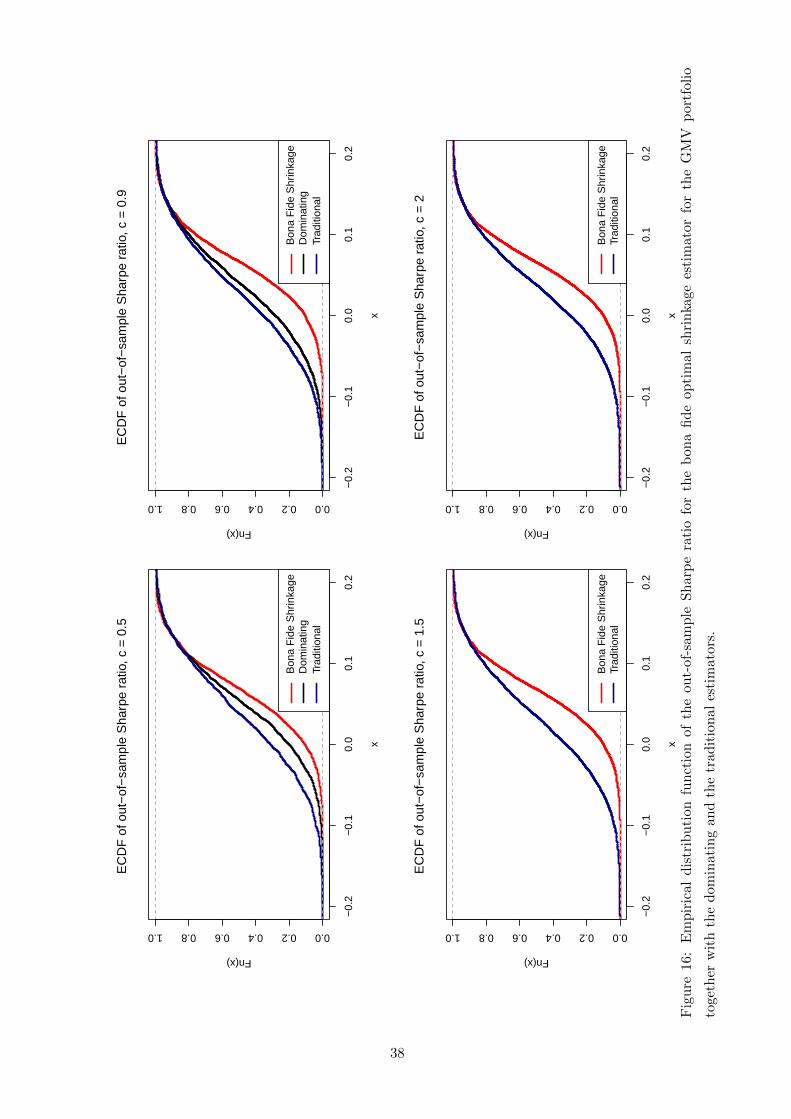
−0.

2−

0.1

0.0

0.1

0.2

0.00.20.40.60.81.0

EC

DF

of o

ut−

of−

sam

ple

Sha

rpe

ratio

, c =

0.5

x

Fn(x)

Bon

a F

ide

Shr

inka

geD

omin

atin

gTr

aditi

onal

−0.

2−

0.1

0.0

0.1

0.2

0.00.20.40.60.81.0

EC

DF

of o

ut−

of−

sam

ple

Sha

rpe

ratio

, c =

0.9

x

Fn(x)

Bon

a F

ide

Shr

inka

geD

omin

atin

gTr

aditi

onal

−0.

2−

0.1

0.0

0.1

0.2

0.00.20.40.60.81.0

EC

DF

of o

ut−

of−

sam

ple

Sha

rpe

ratio

, c =

1.5

x

Fn(x)

Bon

a F

ide

Shr

inka

geTr

aditi

onal

−0.

2−

0.1

0.0

0.1

0.2

0.00.20.40.60.81.0

EC

DF

of o

ut−

of−

sam

ple

Sha

rpe

ratio

, c =

2

x

Fn(x)

Bon

a F

ide

Shr

inka

geTr

aditi

onal

Fig

ure

16:

Em

pir

ical

dis

trib

uti

onfu

nct

ion

ofth

eou

t-of

-sam

ple

Sh

arp

era

tio

for

the

bon

afi

de

opti

mal

shri

nka

ge

esti

mato

rfo

rth

eG

MV

port

foli

o

toge

ther

wit

hth

ed

omin

atin

gan

dth

etr

adit

ional

esti

mat

ors.

38

estimation of the global minimum variance portfolio in ... · portfolio, the global minimum...

Documents