experimental investigation of gsm 900mhz … · progress in electromagnetics research, vol. 125,...

Progress In Electromagnetics Research, Vol. 125, 559–581, 2012

EXPERIMENTAL INVESTIGATION OF GSM 900 MHzRESULTS OVER NORTHERN INDIA WITH AWAS ELEC-TROMAGNETIC CODE AND OTHER PREDICTIONMODELS

M. V. S. N. Prasad1, *, P. K. Dalela2, and C. S. Misra3

1CSIR-National Physical Laboratory, Dr. K S Krishnan Road, NewDelhi 110012, India2C-DOT, Mandigaon Road, Opp. New Manglapuri, Chatterpur,Mehrauli, New Delhi 110030, India3Aircom International Pvt Ltd., Gurgaon 122001, India

Abstract—Recent trends in propagation modeling indicate thestudy of mobile radio propagation modeling with the help ofelectromagnetic formulations which traditionally has been explainedwith empirical methods. These empirical methods were preferred bythe cellular operators in their radio planning tools due to their easeof implementation and less time consumption. In the present study,AWAS electromagnetic code and conventional prediction methods havebeen employed to explain the observed results of ten base stationsmainly in the near field zones of GSM 900 MHz band situated in theurban and suburban regions around Delhi in India. The suitability ofthe above models in terms of prediction errors and standard deviationsare presented. Path loss exponents deduced from the observed datahave been explained by Sommerfeld’s formulations.

1. INTRODUCTION

In order to design high quality and high capacity cellular networks,a thorough understanding of propagation channel is necessary, andsignal strength measurements should be conducted to delineate cellradii and assess reliable coverage area [1]. It is established thatpropagation phenomena can cause unexpectedly poor performancein cellular networks. These are manifested in reduced coverage,

Received 30 December 2011, Accepted 25 February 2012, Scheduled 12 March 2012* Corresponding author: M. V. S. N. Prasad ([email protected]).

560 Prasad, Dalela, and Misra

dropped calls and unexpected hand overs [2]. The performance of thecellular network can be assessed, or new networks can be designedwhen different models are tested with observed results. Arijit Deet al. pointed out [3] that in cellular communication scenario notmuch attention is paid to the relationship between the height of thetransmitting antenna and the distance of transition from near field tofar field region. In the near field, the strength of the field oscillateswildly with large nulls and peaks. They indicated that larger was theheight of transmitting antenna, greater would be the near field region,and the performance of cellular communication systems was degradedappreciably in near field region rather than in the far field region.They positioned the antenna closer to ground and also deployed ahorizontally polarized antenna for mobile communications as the fieldsradiated by a horizontally polarized antenna not to vary too muchwith the height of the antenna in the near field region. Gutierrez-Meana et al. [4] used deterministic radio electric coverage tool for thecomputation of electromagnetic fields based on modified equivalentcurrent approximation method. They illustrated the applicability in arural scenario, where a GSM base station at 900MHz is located, andan urban scenario to test the acceleration technique.

Most of the statistical propagation models used in radio planningtools for the design of cellular radio networks refer to the periodof GSM where antennas are located far above the roof top, andcells were large [5]. Latest developments in mobile radio technologyand introduction of smaller cells, lower antennas necessitated thedevelopment of models applicable to many situations. The specialfeature in Delhi urban environment is that most of the buildingsare non uniformly spaced, and results reported elsewhere might notbe totally applicable to this type of environment. In this context,it is worthwhile to investigate how numerical electromagnetic codescompete with the statistical propagation models in the 900 MHz band.Prasad et al. reported the investigation of eleven base station results inthe 1800 MHz band with AWAS code and other models [6]. To verifythe suitability of AWAS electromagnetic code in the 900 MHz band,field strength measurements were conducted utilizing the followingGSM base stations situated in national capital region of Delhi. Theyare 1. Paschimvihar (PVR) 2. University Area (UA) 3. Nandanagari-1(NN-1). 4. Nandanagari-2 (NN-2) 5. Satyaniketan (SNT) 6. Faridabad(FBD) 7. Vinayak Hospital (VKH) in the urban region and threesuburban base stations namely 1. Tradex tower (TXT), 2. Meethapur(MTR) 3. Gurgaon (GRN). The measured values of signal strengthhave been compared with the prediction methods of AWAS, Hata,COST 231 Walfisch & Ikegami, Dmitry and ITU-R. The models have

Progress In Electromagnetics Research, Vol. 125, 2012 561

been chosen so that they are applicable to the environments wheremeasurements were conducted.

2. ENVIRONMENTAL DESCRIPTIONS

1. Both the NN-1 and NN-2 base stations are surrounded by denseurban areas on three sides and medium urban environment onthe other side. The average building height is around 6 to 9 m.PVR base station is surrounded by medium urban environmentwith slight open areas in between. Far away from the base stationon the left side, low tree density is seen. On the southern sideof the base station, a small water canal flows. UA base stationis surrounded by medium urban environment, and from east tosouth of the base station, a thick patch of tree density is seen.At a distance 2 km away from the base station, dense urbanenvironment prevails on the southern side of the base station.

(a)

(b)


(c)

(d)

Figure 1. (a) Photographs of the environment. (b) Photographs ofthe environment. (c) Photographs of the environment. (d) Googlemap showing the locations of base stations.

MPR base station is surrounded by low density urban area (mainlysuburban) with small patches of green vegetation in between.SNT base station is surrounded by medium urban environmentand small patches of greenery in between, denoting some kindof low urban residential environment. Figures 1(a) to 1(c) showthe photographs of the environment where measurements wereconducted. A google map showing the locations of 10 base stationsis shown in Figure 1(d). The three photographs in Figures 1(a) to1(c) were taken from the close surrounding area of base stationsVKH, FBD and SNT. Since the environmental features of otherbase stations are more or less similar, they are described in detail.


3. EXPERIMENTAL DETAILS

The transmitting power of all base stations is 43.8 dBm, andtransmitting gain is 2 dBi for all base stations except GRN base stationwhere it is 8 dBi. The gain of the receiving antenna is 0 dB and theheight 1.5m. The height of the base station above the ground level andco-ordinates of the base stations are shown in Table 1. The receiver isstandard Nokia equipment used in drive in tools for field trials. Theposition of the mobile is determined from the GPS receiver, and thisinformation with the co-ordinates of the base station was utilized todeduce the distance traveled by the mobile from the base station. Thesignal strength information recorded in dBm was converted into pathloss values utilizing the gains of the antenna. The data were recordedwith 512 samples in one second on a laptop, and the number of samplescollected for each site varied from 1× 105 to 2× 105. Measured r.m.s.error is around 1.5 dB. Data were averaged over conventional figure of40λ.

4. PREDICTION METHODS

The following prediction methods have been utilized in this study.1. AWAS numerical code based on electromagnetic modeling [7].

Table 1. Details of base stations used in the study.

Urban

regionhb (m) Lat (deg) Long (deg)

Maximum Near

field Distance (m)

PVR 13 28.6738 77.08882 236

UA 24 28.69655 77.21367 436

NN-1 14 28.66912 77.36256 220

NN-2 12 28.68908 77.3026 189

SNT 18 28.58845 77.16848 284

FBD 10 28.38071 77.29720 158

VKH 13 28.57132 77.32809 205

Suburban

region

TXT 43 28.47266 77.51447 678

MTR 12 28.49434 77.32450 189

GRN 20 28.4753 77.08445 315

hm = 1.5


2. ITU-R method [8]. 3. Dmitry model [9]. 4. COST 231 Walfisch-Ikegami method [10]. 5. Hata method [11].

4.1. AWAS Numerical Electromagnetic Code

AWAS electromagnetic code has been utilized to compare thepredictions in the near field and far field zones. It is utilized to computethe path loss values with different values of dielectric constant andconductivity of 2× 10−4 over real ground. The commercially availablecomputer program is capable of analyzing wire antennas operating intransmitting and receiving modes as well as analyzing wire scatterers.Different values of dielectric constant for dense urban, urban andsuburban regions have been incorporated in the computation of AWASsimulation. Reference [12] gives dielectric constants for various typesof grounds and environments. It gives values of 3–5 for city industrialarea. Hence a value of 4 is used in the simulation of AWAS for denseurban base stations. The same reference gives a value of 10 for fertilelands and a value of 15 for agricultural lands. In the present studythere is no region of fertile land and agricultural lands, but urban andsuburban regions. In this study, the type of ground is the same inthe case of all base stations, and the difference in urban and suburbanregions comes from the degree of urbanization. In [13], a value of4 for dielectric constant has been chosen for urban region when realearth is considered with imperfectly conducting ground. Keeping theseaspects in view, we have carefully chosen a value of 6 for urban basestations and a value of 8 for suburban base stations in the AWASsimulation. The technique is based on the two-potential equation forthe distribution of wire currents. This integro–differential equation issolved numerically using the method of moments with a polynomialapproximation for the current distribution. The influence of groundis taken into account using Sommerfeld’s approach with numericalintegration algorithms developed exclusively for this program. Theprogram evaluates the fields in the near and far field regions, and thefields were converted into path losses to compare with the observedvalues.

4.2. ITU-R Model

ITU-R recommendation 1411-4 provides prediction capability foroutdoor short range radio communication systems and radio local areanetworks in the frequency range 300 MHz–100 GHz and gives closed-form algorithms both for site-specific and site-general calculations.The model is applicable to urban high rise, low rise urban, suburban,residential and rural areas. In the case of dense urban or urban under


nlos (non line-of-sight) category the range of applicability of this modelis, base station antenna height (hb) from 4 to 50 m, mobile antennaheight (hm) from 1 to 3 m, frequency (f) from 800 to 5000 MHz, and2 to 16 GHz for hb <hm and distance (d) from 20 to 5000 m. In thecase of suburban regions, any height of hm can be used, ∆ hb from 1 to100m (∆ hb is the difference of base station and average roof heights),∆ hm from 4 to 10 m (∆ hm is the difference of roof height and mobileheights), street width (w) ranging from 10 to 25 m and d from 10 to5000m. Multiscreen diffraction terms are incorporated to account theroof top diffractions in the urban zone. Here the average roof topheight is used. In the nlos category for roof tops of similar height, theloss is expressed as sum of free space loss, multiscreen diffraction lossand loss due to coupling of wave propagation along the multiscreenpath into the street where mobile is located. Here width of the streetis taken into consideration. For more details the reader can refer toITU-R recommendation. In the case of suburban zones propagationmodel based on geometrical optics is given.

4.3. Dmitry Model

Dmitry method comes under stochastic category. In the case ofDmitry method, propagation modeling is done by explicitly consideringrandom diffuse scattering at street level in the vicinity of the mobileand propagation over clutter as a deterministic problem. The authorscompare their model over an urban environment with COST 231 Hata,Walfisch-Bertoni models at 2GHz, for base station antenna heightof 25m, clutter height of 20m and street width of 30m and mobileantenna height of 2 m. In another study Yarkoni et al. [14] investigatedthe total received signal for mobile antenna in urban region basedon multi parametric stochastic approach. They claimed that theirequations can predict different propagation situations and path loss invarious urban channels for different heights of base station and mobileterminal antennas.

4.4. Walfisch-Ikegami (WI) Method

Walfisch-Ikegami (WI) method is one of the most widely usedanalytical models to predict the path loss which consists of acombination of Walfisch and Ikegami models. Here the path loss isa combination of free space loss, multiple knife-edge diffraction to thetop of the final building and single diffraction and scattering processdown to street level. The model is applicable to frequencies between800 to 2000 MHz; hb between 4 and 50 m, hm between 1 and 3 m, anddistances between 200 to 5000 m. Performance of the model is poor


when hb is less than hm. In the present study, this model is utilizedfor street width of 20 m and roof heights of 12 and 15 m.

4.5. Hata Method

The well-known Hata model is a fully empirical model based entirelyupon extensive series of measurements made in Tokyo City between200MHz and 2 GHz [11]. Different equations are available for urban,suburban and open zones.

Figure 2. Comparison of observed path loss values with variousmodels for PVR base station.

Figure 3. Comparison of observed path loss values with variousmodels for UA base station.


Figure 4. Comparison of observed path loss values with variousmodels for NN-1 base station.

Figure 5. Comparison of observed path loss values with variousmodels for NN-2 base station.

5. RESULTS

The comparison of the above prediction methods with observed valuesof path loss for base stations PVR, UA, NN-1, NN-2, SNT, FBD,VKH,TXT, MTR and GRN base stations are shown in Figures 2–11. Theending of the near field distances designated as near field maximumcomputed for all the base stations are shown in Table 1. The maximumnear field distance has been computed using the formula 4hb hm/λtaken from the extensive discussion on near and far field effects oncellular communication systems from the work of Arijit De et al. [3].


Figure 6. Comparison of observed path loss values with variousmodels for SNT base station.

The variations in the near field are more important than in the farfield since the observed path loss of cellular communication systemin near field region shows large variations. In Figure 2, close tothe transmitter below 500 m, the observed values of path loss varybetween 80 to 140 dB, showing large dispersion of path loss values, andbeyond 500 m, are confined between 100 and 150 dB. Beyond 500 m,the path loss has less dispersion. AWAS numerical code and Hatamethod for urban regions show good agreement with the observedvalues. ITU-R (nlos) overestimates the observed values beyond 500 m.Path loss curves of Dmitry and WI methods pass through the lowerpart of the observed path loss values. ITU-R (los) method appreciablyunderestimates especially in the region below 1000 m. In Figure 3for UA base station observed values below 500 m vary between 80 to130 dB, and large dispersion of path loss is seen in this region. Beyond500m, path loss is confined between 90 and 135 dB up to 2500m.Similar to Figure 2, AWAS and Hata methods give good agreement.Predicted path loss graphs of Dmitry and WI methods pass through thelower half of the observed path loss patch; ITU-R (los) passes throughthe lower part of observed loss; ITU-R (nlos) passes through the upperregion of observed loss. At a given distance, the observed loss variesapproximately by 20 dB. In fact, both the curves can be used to predictthe variability of path loss. More or less similar trend is seen for theremaining Figures 4 to 11 for the other base stations. Some interestingfeatures observed in these figures are described below.

In Figures 4 & 5 for NN-1 and NN-2 base stations, observed lossbelow 500m is moderately higher than those in Figures 2 and 3 dueto very narrow street widths and congested urban settings (buildings


Figure 7. Comparison of observed path loss values with variousmodels for FBD base station.

Figure 8. Comparison of observed path loss values with variousmodels for VKH base station.

are non uniform also). Hence AWAS and Hata methods appear topass through the lower half of observed path loss patch. ITU-R (los)and Dmitry methods underestimate by 20 to 25 dB. In Figure 5, theobserved losses below 200 m are higher than that of Figure 4 probablydue to the location of base station in zones where street widths arenarrower than that of Figure 4’s base station. In Figures 6 & 7, for SNTand FBD base stations variation of observed path loss is similar to Figs.2 & 3. Observed path loss varies between 80 to 120 dB below 500 m andbeyond this varies between 90 to 140 dB. Prediction methods AWAS,


Figure 9. Comparison of observed path loss values with variousmodels for TXT base station.

Figure 10. Comparison of observed path loss values with variousmodels for MTR base station.

Hata and WI give good agreement with the observed loss whereas thatof Dmitry and ITU-R(los) pass through the lower side of observed pathloss patch. ITU-R (nlos) method overestimates appreciably. Lowerobserved path loss values are probably due to wider street width andmore or less uniform structure of buildings yielding less losses thanthose of Figures 4 & 5. Figure 8 exhibits variations similar to Figure 7due to similarities in urban structure.

In the case of Figure 9, the observed path loss varies between 80to 120 dB below 500 m and beyond that 90 to 120 dB up to 4000 m.Beyond break point path loss getting confined to a range of values


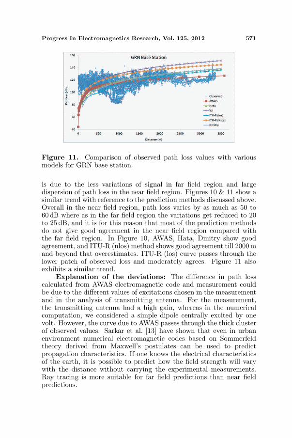
Figure 11. Comparison of observed path loss values with variousmodels for GRN base station.

is due to the less variations of signal in far field region and largedispersion of path loss in the near field region. Figures 10 & 11 show asimilar trend with reference to the prediction methods discussed above.Overall in the near field region, path loss varies by as much as 50 to60 dB where as in the far field region the variations get reduced to 20to 25 dB, and it is for this reason that most of the prediction methodsdo not give good agreement in the near field region compared withthe far field region. In Figure 10, AWAS, Hata, Dmitry show goodagreement, and ITU-R (nlos) method shows good agreement till 2000 mand beyond that overestimates. ITU-R (los) curve passes through thelower patch of observed loss and moderately agrees. Figure 11 alsoexhibits a similar trend.

Explanation of the deviations: The difference in path losscalculated from AWAS electromagnetic code and measurement couldbe due to the different values of excitations chosen in the measurementand in the analysis of transmitting antenna. For the measurement,the transmitting antenna had a high gain, whereas in the numericalcomputation, we considered a simple dipole centrally excited by onevolt. However, the curve due to AWAS passes through the thick clusterof observed values. Sarkar et al. [13] have shown that even in urbanenvironment numerical electromagnetic codes based on Sommerfeldtheory derived from Maxwell’s postulates can be used to predictpropagation characteristics. If one knows the electrical characteristicsof the earth, it is possible to predict how the field strength will varywith the distance without carrying the experimental measurements.Ray tracing is more suitable for far field predictions than near fieldpredictions.


6. STANDARD DEVIATIONS OF THE PREDICTIONMETHODS

Based on the above comparison, prediction errors of the models havebeen deduced where prediction error is given by the difference of theobserved and predicted values. Standard deviations of all the basestations for the above methods have been calculated and are shown inTable 2. In the table, ME refers to mean error and SD to standarddeviation. In the case of AWAS the lowest standard deviation of 8.1is seen for PVR base station and the highest value of 23.2 for NN-2base station. The average value of standard deviation for all urbanbase stations is 12.78 and for suburban stations is 13.6. In the case of

Table 2. Standard deviations and mean errors (in dB) of theprediction methods.

Basestation

AWASME SD

HataME SD

WIME SD

PVR 0.3 8.1 −2.5 11.0 0.8 11.0UA −1.8 9.5 −3.4 10.5 2.0 10.6

NN-1 5.0 9.7 3.5 10.4 0.6 10.2NN-2 7.5 23.2 7.3 13.8 2.4 12.8SNT 2.2 12.3 0.5 12.9 −0.7 13.0FBD −1.4 12.2 −5.6 13.2 −4.8 12.5VKH −6.3 14.5 −9.2 21.6 −6.0 16.0TXT −19.1 16.3 −16.0 16.8 −14.5 17.2MTR −2.4 12.8 −0.2 14.3 −14.9 17.5GRN 0.5 11.7 −2.9 14.3 −13.8 16.7Base

stationITU-R(los)

ME SDITU-R(nlos)

ME SDDmitryME SD

PVR 6.8 12.3 −11.3 12.3 4.3 10.8UA 6.3 10.8 −9.8 12.3 5.9 11.4

NN-1 15.6 13.4 −4.8 10.8 14.0 13.3NN-2 21.2 16.1 −3.6 12.8 15.9 14.7SNT 8.0 14.1 −9.7 14.9 9.3 14.8FBD −22.0 20.3 -32.3 16.4 0.3 12.8VKH −1.0 14.9 −21.5 18.4 −2.4 15.4TXT −3.1 16.3 −20.5 18.3 −4.3 15.2MTR 1.3 14.7 −13.5 16.4 −1.5 15.3GRN 0.17 14.1 −9.8 14.7 −2.3 15.0


Hata method, the lowest value of 10.5 for UA base station and 10.4 forNN-1 base station and highest value of 21.6 for VKH base station areobserved. The average value of standard deviation for all urban basestations is 13.34 and for suburban stations is 15.13. WI also follows asimilar trend, and the average value of standard deviation for all theurban base stations is 12.13 and for suburban base stations is 17.13.In the case of ITU-R (los), average value for urban base stations is14.55 and for suburban base stations is 15.03. For ITU-R (nlos) andDmitry, the corresponding values are 13.98 and 13.31 for urban basestations and 16.46 and 15.16 for suburban base stations, respectively.From the above discussion, it appears that AWAS numerical code hasa slight edge over others followed by Hata and WI methods.

7. PATHLOSS EXPONENTS

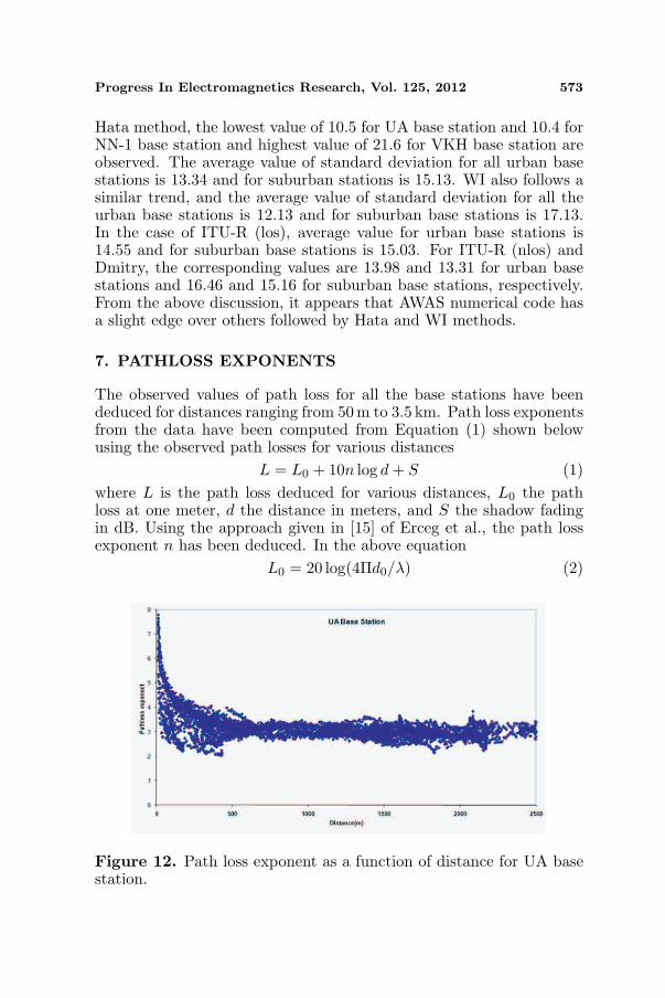
The observed values of path loss for all the base stations have beendeduced for distances ranging from 50 m to 3.5 km. Path loss exponentsfrom the data have been computed from Equation (1) shown belowusing the observed path losses for various distances

L = L0 + 10n log d + S (1)where L is the path loss deduced for various distances, L0 the pathloss at one meter, d the distance in meters, and S the shadow fadingin dB. Using the approach given in [15] of Erceg et al., the path lossexponent n has been deduced. In the above equation

L0 = 20 log(4Πd0/λ) (2)

Figure 12. Path loss exponent as a function of distance for UA basestation.


where λ is the wavelength corresponding to 900MHz, and d0 is takenas one meter. S is the shadow fading variation, varies from locationto another within given macrocell, and tends to be Gaussian in agiven macro cell denoting shadow fading as lognormal. It can beexpressed as s = yσ, where y is a zero mean Gaussian variable ofunit standard deviation, and σ the standard deviation of S is itself aGaussian variable over macrocells. L is taken from the observed pathloss values. Using the above values, the path loss exponent ‘n’ hasbeen deduced and shown in Figures 12–15 for some base stations UA,SNT, FBD and VKH. In all these diagrams, the exponent close totransmitter exhibits higher values of the order of 8, falls steeply andstabilizes to a value of around 3, and remains the same for the restof the distances denoting stable values in the far field zone. Thesefigures have great significance in delineating near and far field regionsfrom the observed data and can serve as design inputs for fixing theboundaries of cell radii. Closer is the transition point of near fieldto far field zone to the transmitter, better will be the performance ofcellular communication network.

It is well known that in the near field regions the path lossexponent is 3 due to the static nature of the fields. The pathloss exponent should be around 6 as there is no static nature in it.Figures 12–15 showing the variation of path loss exponent as a functionof distance depict high path loss exponent values at distances close totransmitter, and they fall steeply till the end of near field zone. Beyondthese values, the exponent remains more or less stable. In the path loss

Figure 13. Path loss exponent as a function of distance for SNT basestation.


Figure 14. Path loss exponent as a function of distance for FBD basestation.

Figure 15. Path loss exponent as a function of distance for VKH basestation.

exponent diagrams (Figures 12–15), the curve turns at an exponentof 4 and stabilizes with a value of 3 for the remaining distancescalled intermediate distances. Sarkar [16] through accurate numericalanalysis using Sommerfeld formulations showed that at distances veryfar away from the base station (beyond intermediate distances), theexponent starts increasing to a value of 4. Figures 12–15 depict up tointermediate distances where the exponent gets stabilized to a value of3, in accordance with the Sommerfeld’s propositions. In other words,the present data substantiated many of the Sommerfeld’s findings, andphysics based macro modeling would be sufficient to explain many of


the observed results.Sarkar et al. [13] have shown that when antenna is placed on the

top of a cellular tower, it produces highly undesirable radiation pattern.Moreover, the signal strength goes through a series of maxima andminima even though the antenna is located and radiating in free space.

This type of radiation pattern for a dipole transmitting antenna isnatural due to interference between the fields from the original dipolewith its image created by the presence of ground and not due tothe buildings as no building parameters are present in AWAS. If theantenna is located at 100m or above as in a microwave line-of-sightlink, lobing effects in the pattern will be minimized as the strength ofimage will be reduced due to losses in the ground. Sommerfeld’s theorypredicts that the effects of surface wave will be minimal as one goesaway from the antenna and that the interference between the spacewave and surface wave will be less reducing the lobing effects in thepattern. This has been exhibited by the above discussed path lossexponent diagrams with variations coming strongly in the near fieldregion due to the antenna heights situated between 20–30 m.

8. BREAK POINT DISTANCES

The break point has been deduced as the distance at which the slope ofthe curve (the path loss exponent vs distance) changes. In Figure 12,it changes at 300 m. Observed break point has been taken from thediagrams showing the variation of path loss exponent as a functionof distance and shown in Table 3. An examination of these path lossexponent curves shows that at distances close to transmitter, exponentfalls rapidly from higher values, and the slope of the curve changes at

Table 3. Break point distances observed from data.

Base station Height of tx. ant (m) Observed break point (m)

1. PVR 13 300

2. UA 24 300

3. NN-1 14 200

4. NN-2 12 200

5. SNT 18 300

6. FBD 10 300

7. VKH 13 300

8. TXT 43 400

9. MTR 12 250

10. GRN 20 500


a particular distance. We have reported these distances at which theslope of the curve changes as the break point for various base stations.The end of the near field or maximum near field distance representsthe end of the region where rapid variations of signal are seen. Beyondthe maximum near field distance, far field region starts where the pathloss exponent is more or less stabilized. In the far field region, onlyheight gain of antenna is seen.

Examination of the above table shows that the position of thebreak point distance depends not only on the height of the base stationantenna, but also on the type of terrain and environment surroundingthe base station. In the case of suburban base stations for the sameantenna height, the break point is larger than the correspondingstations in the urban zone. For example, in the case of SNT basestation with antenna height of 18 m, the break point is found at 300mwhereas in the suburban region base station GRN with antenna heightof 20m, the break point is found at 500 m. In urban environment, thebreak point is seen at smaller distances which could be due to highdensity of urbanization.

Discussion: In the case of [15] by Erceg et al., who madeextensive measurements at 1.9 GHz at New Jersey, Seattle andChicago, high path losses close to the transmitter were observed, andthen the loss decreased linearly with distance. In the present study, thepath loss is falling steeply up to 0.5 km. The nature of variation of pathloss exponent in the present study resembled the variation in Erceg etal.’s study. Steep transitions of path loss occur when the base stationantenna height is close to the height of surrounding building roof tops.Hence the height accuracy of the base station antenna is especiallysignificant if large prediction errors are to be avoided [17]. Milanovicet al. [18] have observed that in dense urban regions measurementsshow a very interesting feature. Path loss after the break point doesnot increase with distance, probably due to the wave guiding effect ofcity streets as well as the existence of radio wave components reflectedand diffracted on buildings reaching the receiver antenna. The pathloss exponent in the present study showed this trend. Herring etal. [19] observed a large variance in received power as a function ofdistance. This showed that using a single value of path loss exponentfor a particular neighbourhood as assumed in popular empirical modelscan lead to large errors in path loss estimates. High path losses close tothe transmitter require higher margins from operators. The deviationof all the prediction methods at closer distances to the transmitter ishigh due to the large path loss variation.

Another advantage of studying path loss exponent as a functionof distance is the identification of exclusion zones. These are the


zones around base stations within which emf’s exposure guide lines areexceeded in order to protect the general public from potential harmfullevels of radiation [20]. In the reactive near field, radiative near andfar field regions around base station, radiated field does not presentthe same behavior, and adequate propagation models are required toestimate the exact field strength at any specific distance. Typically,exclusion zones around base station antennas, inside which exposurethresholds may be exceeded, are in the near field zone of radiatingantenna (some meters).

Baltzis [21] showed that path loss cumulative distribution functionwas dependent on path loss exponent and system geometry. Effect ofwet forest on the deployment of Zigbee network has been investigatedby Gay-Fernandez et al. [22], and Helhel et al. [23] investigated dryand wet earth effects on GSM 900&1800 MHz propagation in Turkey.Phaiboon and Phokharatkul [24] using modified Xia model investigated900&1800MHz measurements. Pu et al. [25] estimated small scalefading characteristics of RF wireless link under railway communicationenvironment. For next generation wide band communication systemsspectrum efficiency could be increased, and signal quality could beimproved with the implementation of co-ordination scheme amongbase stations [26]. Three dimensional ray tracing methods in urbanmicrocellular environments have been utilized by Liu and Guo [27].

9. CONCLUSIONS

In the present study, the observed path losses from 10 base stationsoperating in the GSM 900MHz band situated in the urban andsuburban regions of Delhi have been compared with the AWASelectromagnetic code and conventional prediction methods, such asHata, WI, Dmitry and ITU-R. Overall AWAS, Hata & WI curvesshow good agreement with the observed values. These curves passthrough the centre of the observed cluster of path losses. In the nearfield region, AWAS predicts the observed values better than Hata& WI methods. In the suburban/low density urban regions, ITU-R(nlos) curve overestimates path losses by 20 dB. The average values ofstandard deviations reported by AWAS are 12.78 and 13.6 for urbanand suburban base stations with Hata showing 13.34 and 15.13 and WI12.13 and 17.13, respectively. AWAS numerical code has shown moreor less the same deviation in urban and suburban regions, is suitablefor any type of environment, and does not require any tuning of thecoefficients unlike other methods. The difference in standard deviationsfor other methods ranges from 3–5 dB for urban and suburban regions.From the observed path losses values, path loss exponents as a function


of distance have been calculated, and from these curves break pointdistances have been deduced. These have been explained in termsof transitions between near and far field zones. Higher path lossesobserved in the near field zones of base stations require novel strategiesto improve the performance of cellular networks.

REFERENCES

1. Nadir, Z. and M. I. Ahmad, “Pathloss determination usingOkumara-Hata model and cubic regression for missing data forOman,” Proc. of the International Multi Conference of Engineersand Computer Scientists, IMECS 2010, Vol. 11, 804–807, HongKong, Mar. 17–19, 2010.

2. Kwakkernaat, M. R. J. A. E. and M. H. A. J. Herben, “Diagnosticanalysis of radio propagation in UMTS networks using highresolution angle-of-arrival measurements,” IEEE Antennas andPropagation Magazine, Vol. 53, No. 1, 66–75, Feb. 2011.

3. De, A., T. K. Sarkar, and M. Salazar-Palma, “Characterizationof the far field environment of antennas located over a groundplane and implications for cellular communication systems,” IEEEAntennas and Propagation Magazine, Vol. 52, No. 6, 19–40,Dec. 2010.

4. Gutierrez-Meana, J., J. A. Martinez-Lorenzo, F. Las-Heras, andC. Rappaport, “DIRECT: A deterministic radio coverage tool,”IEEE Antennas and Propagation Magazine, Vol. 53, No. 2, 135–145, Apr. 2011.

5. Mantel, O. C., J. C. Oosteveen, and M. P. Popova, “Applicabilityof deterministic propagation models for mobile operators,” SecondEuropean Conf. on Antennas and Propagation, Eucap 2007, 11–16, Nov. 2007, Print ISBN. 978-0-86341-842-6.

6. Prasad, M. V. S. N., S. Gupta, and M. M. Gupta, “Compari-son of 1.8 GHz cellular outdoor measurements with AWAS elec-tromagnetic code and conventional models over urban and subur-ban regions of northern India,” IEEE Antenna and PropagationMagazine, Vol. 53, No. 4, 76–85, Aug. 2011.

7. Djordjevic, A. R., M. B. Bazdar, T. K. Sarkar, and R. F. Harring-ton, AWAS for Windows Version 2.0: Analysis of Wire Antennasand Scatterers, Software and User’S Manual, Artech House, 2002,ISBN: 1-58053-488-0.

8. ITU-R, P.1411-4, “Propagation data and prediction methods forthe planning of short-range outdoor radio communication systems


and radio local area networks in the frequency range 300MHz to100GHz,” International Telecommunication Union, Geneva, 2001.

9. Chizhik, D. and J. Ling, “Propagation over clutter: Physicalstochastic model,” IEEE Trans. on Antennas and Propagation,Vol. 56, No. 4, 1071–1077, Apr. 2008.

10. Erceg, V, K. V. S. Hari, M. S. Smith, D. S. Baum, K. P. Sheikh,C. Tappenden, J. M. Costa, C. Bushue, A. Sarajedini,R. Schwartz, D. Branlund, T, Kaitz, and D. Trinkwon, “Channelmodels for fixed wireless applications,” Contribution IEEE P802.16 3C-01/29r4, IEEE 802.16, 2003.

11. Hata, M., “Empirical formula for propagation loss in land obileradio services,” IEEE Trans.Veh.Tech., Vol. 29, 317–325, 1980.

12. Soil dielectric properties (Dielectric materials and applica-tions), NEC list, and website: pe2bz.philpem.me.uk/Comm/-%20Antenna/.../soildiel.htm.

13. Sarkar, T. K., S. Burintramart, N. Yilmazer, S. Hwang, Y. Zhang,A. De, and M. Salazar-Palma, “A discussion about someof the principles/practices of wireless communication under aMaxwellian framework,” IEEE Transactions on Antennas andPropagation, Vol. 54, No. 12, 3727–3745, Dec. 2006.

14. Yarconi, N., N. Blaunstein, and D. Katz, “Link budget andradio coverage design for various multipath urban communicationlinks,” RadioScience, Vol. 42, RS2009, 1–15, 2007.

15. Erceg, V., S. Y. Tjandra, S. R. Parkoff, G. Ajay, K. Boris,A. A. Julius, and B. Renee, “An empirically based path loss modelfor wireless channels in suburban environments,” IEEE Journal onSelected Areas in Communs., Vol. 17, No. 7, 1205–1211, Jul. 1999.

16. Sarkar, T. K., “Near and far field antennas,” Organized session oncommunications, IEEE Conf. on Applied Electromagnetics, 18–22,Kolkata, India, Dec. 2011.

17. Michaelides, C. P. and A. R. Nix, “Accurate high speed urban fieldstrength predictions using a new hybrid statistical deterministicmodeling technique,” 54th Vehicular Technology Conf., Vol. 2,1088–1092, Atlanta, NJ, USA, Oct. 7–11, 2001.

18. Milanovic, J., D. Rimac, and K. Bejuk, “Comparison ofpropagation models accuracy for wimax on 3.5 GHz,” ICECS2007, 14th IEEE International Conf. on Electronics Circuits andSystems, 111–114, Dec. 11–14, 2007.

19. Herring, K. T., J. W. Holloway, D. H. Staelin and D. W. Bliss,“Path loss characteristics of urban wireless channels,” IEEETransactions on Antennas and Propagation, Vol. 58, No. 1, 171–


177, Jan. 2010.20. Sebastiao, D., D. Ladeina, M. Antunes, C. Oliveire, and

L. M. Correia, “Estimation of base station exclusion zones,” VTC2010 Fall, 1–5, Ottawa, Sept. 6–9, 2010.

21. Baltzis, K. B., “A geometric method for computing thenodal distance distribution in mobile networks,” Progress InElectromagnetics Research, Vol. 114, 159–175, 2011.

22. Gay-Fernandex, J. A., M. Garcia Sanchez, I. Cuinas, A. V. Alejos,J. G. Sanchez, and J. L. Miranda-Sierra, “Propagation analysisand deployment of a wireless sensor network in a forest,” ProgressIn Electromagnetics Research, Vol. 106, 121–145, 2010.

23. Helhel, S., S. Ozen, and H. Goksu, “Investigation of GSMsignal variation depending weather conditions,” Progress InElectromagnetics Research B, Vol. 1, 147–157, 2008.

24. Phaiboon, S. and P. Phokharatkul, “Path loss prediction for low-rise buildings with image classification on 2-D aerial photographs,”Progress In Electromagnetics Research, Vol. 95, 135–152, 2009.

25. Pu, S., J.-H. Wang, and Z. Zhang, “Estimation for small-scale fad-ing characteristics of RF wireless link under railway communica-tion environment using integrative modeling technique,” ProgressIn Electromagnetics Research, Vol. 106, 395–417, 2010.

26. Tseng, H.-W., Y.-H. Lee, J.-Y. Lin, C.-Y. Lo, and Y.-G. Jan, “Performance analysis with coordination among basestations for next generation communication systems,” Progress InElectromagnetics Research B, Vol. 36, 53–67, 2012.

27. Liu, Z.-Y. and L.-X. Guo, “A quasi three-dimensional ray tracingmethod based on the virtual source tree in urban microcellularenvironments,” Progress In Electromagnetics Research, Vol. 118,397–414, 2011.

experimental investigation of gsm 900mhz … · progress in electromagnetics research, vol. 125,...

Documents