exploring and measuring non-linear correlations: copulas...
TRANSCRIPT

Journal of Machine Learning Research Volume 55 (2016) 1–11 Submitted submitted; Published published
Exploring and measuring non-linear correlations:Copulas, Lightspeed Transportation and Clustering
Gautier Marti [email protected] Capital LtdEcole Polytechnique
Sebastien Andler [email protected] de LyonHellebore Capital Ltd
Frank Nielsen [email protected] Polytechnique
Philippe Donnat [email protected]
Hellebore Capital Ltd
Editor: Oren Anava, Marco Cuturi, Azadeh Khaleghi, Vitaly Kuznetsov, Alexander Rakhlin
AbstractWe propose a methodology to explore and measure the pairwise correlations that exist betweenvariables in a dataset. The methodology leverages copulas for encoding dependence between twovariables, state-of-the-art optimal transport for providing a relevant geometry to the copulas, andclustering for summarizing the main dependence patterns found between the variables. Some ofthe clusters centers can be used to parameterize a novel dependence coefficient which can targetor forget specific dependence patterns. Finally, we illustrate the methodology with financial timeseries (credit default swaps, stocks, foreign exchange rates). Code and numerical experiments areavailable online at https://www.datagrapple.com/Tech for reproducible research.Keywords: Correlations, Copulas, Regularized Optimal Transport, Financial Time Series
1. Introduction
Pearson’s correlation coefficient which estimates linear dependence between two variables is stillthe mainstream tool for measuring variable correlations in science and engineering. However, itsshortcomings are well-documented in the statistics literature: not robust to outliers; not invariantto monotone transformations of the variables; can take value 0 whereas variables are strongly de-pendent; only relevant when variables are jointly normally distributed. A large but under-exploitedliterature in statistics and machine learning has expanded recently to alleviate these issues (Reshefet al., 2011; Szekely et al., 2009). An underlying idea to many of the dependence coefficients is tocompute a distance D(P (X,Y ), P (X)P (Y )) between the joint distribution P (X,Y ) of variablesX , Y and P (X)P (Y ) the product of marginal distributions encoding the independence. For exam-ple, choosingD = KL (Kullback-Leibler divergence), we end up with the Mutual Information (MI)measure, well-known in information theory. Thus, one can detect all the dependences between Xand Y since the distance will be greater than 0 as soon as P (X,Y ) is different from P (X)P (Y ).Then, the dependence literature focus has shifted toward the new concept of “equitability” (Kin-ney and Atwal, 2014): How can one quantify the strength of a statistical association between two
c©2016 Gautier Marti.
MARTI et al.
variables without bias for relationships of a specific form? Many researchers now aim at designingand proving that their proposed measures are indeed equitable (Ding and Li, 2013; Chang et al.,2016). This is not what we look for in this article. But, on the contrary, we want to target specificdependence patterns and ignore others. We want to target dependence which are relevant to such orsuch problem, and forget about the dependence which are not in the scope of the problems at hand,or even worse which may be spurious associations (pure chance or artifacts in the data). The latterwill be detected with an equitable dependence measure since they are deviation from independence,and will be given as much weight as the interesting ones. Rather than using the biases for specificdependence of several coefficients, we propose a dependence coefficient that can be parameterizedby a set of target-dependences, and a set of forget-dependences. Sets of target and forget depen-dences can be built using expert hypotheses, or by leveraging the centers of clusters resulting froman exploratory clustering of the pairwise dependences. To achieve this goal, we will leverage threetools: copulas, optimal transportation, and clustering. Whereas clustering, the task of grouping aset of objects in such a way that objects in the same group (also called cluster) are more similar toeach other than those in different groups, is common knowledge in the machine learning commu-nity, copulas and optimal transportation are not yet mainstream tools. Copulas have recently gainedattention in machine learning, and several copula-based dependence measures have been proposedfor improving feature selection methods (Ghahramani et al., 2012; Lopez-Paz et al., 2013; Changet al., 2016). Optimal transport may be more familiar to computer scientists working in computervision since it is the underlying theory of the Earth Mover’s Distance (Rubner et al., 2000). Un-til very recently, optimal transportation distances between distributions were not deemed relevantfor machine learning applications since the best computational cost known was super-cubic to thenumber of bins used for discretizing the distribution supports which grows itself exponentially withthe dimension. A mere distance evaluation could take several seconds! In this article, we leveragerecent computational breakthroughs detailed in (Cuturi, 2013) which make their use practical inmachine learning. We demonstrate it by studying a comprehensive dataset of financial time series.To capture their associations, most quantitative approaches make use of an estimated covarianceor correlation matrix (a mixed information of linear dependence perturbed by the possibly heavy-tailed marginals) or a Gaussian copula (which only captures the linear dependence while factoringout properly the marginals). This may have dramatic effect on subsequent analysis: (Marti et al.,2016b) for an example with financial time series clustering. Using the proposed methodology, wecan explore the dependence between these time series.
2. Background on Copulas and Optimal Transport
2.1 Copulas
Copulas are functions that couple multivariate distribution functions to their univariate marginaldistribution functions. In this article, we will only consider bivariate copulas, but most of the re-sults and the methodology presented hold in the multivariate setting, at the cost of a much highercomputational burden which is for now a bit unrealistic.
Theorem 1 (Sklar’s Theorem) Let X = (Xi, Xj) be a random vector with a joint cumulativedistribution function F , and having continuous marginal cumulative distribution functions Fi, Fjrespectively. Then, there exists a unique distribution C such that F (Xi, Xj) = C(Fi(Xi), Fj(Xj)).C, the copula of X , is the bivariate distribution of uniform marginals Ui, Uj := Fi(Xi), Fj(Xj).
2
EXPLORING AND MEASURING NON-LINEAR CORRELATIONS
0 0.5 1
ui
0
0.5
1
uj
w(ui, uj)
0.000
0.002
0.004
0.006
0.008
0.010
0.012
0.014
0.016
0.018
0.020
0 0.5 1
ui
0
0.5
1
uj
W(ui, uj)
0.0
0.1
0.2
0.3
0.4
0.5
0.6
0.7
0.8
0.9
1.0
0 0.5 1
ui
0
0.5
1
uj
π(ui, uj)
0.00036
0.00037
0.00038
0.00039
0.00040
0.00041
0.00042
0.00043
0.00044
0 0.5 1
ui
0
0.5
1
uj
Π(ui, uj)
0.0
0.1
0.2
0.3
0.4
0.5
0.6
0.7
0.8
0.9
1.0
0 0.5 1
ui
0
0.5
1
uj
m(ui, uj)
0.000
0.002
0.004
0.006
0.008
0.010
0.012
0.014
0.016
0.018
0.020
0 0.5 1
ui
0
0.5
1
uj
M(ui, uj)
0.0
0.1
0.2
0.3
0.4
0.5
0.6
0.7
0.8
0.9
1.0
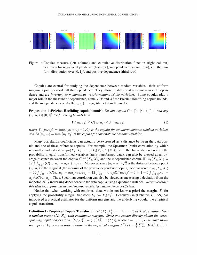
Figure 1: Copulas measure (left column) and cumulative distribution function (right column)heatmaps for negative dependence (first row), independence (second row), i.e. the uni-form distribution over [0, 1]2, and positive dependence (third row)
Copulas are central for studying the dependence between random variables: their uniformmarginals jointly encode all the dependence. They allow to study scale-free measures of depen-dence and are invariant to monotonous transformations of the variables. Some copulas play amajor role in the measure of dependence, namelyW andM the Frechet-Hoeffding copula bounds,and the independence copula Π(ui, uj) = uiuj (depicted in Figure 1).
Proposition 1 (Frechet-Hoeffding copula bounds) For any copula C : [0, 1]2 → [0, 1] and any(ui, uj) ∈ [0, 1]2 the following bounds hold:
W(ui, uj) ≤ C(ui, uj) ≤M(ui, uj), (1)
where W(ui, uj) = max {ui + uj − 1, 0} is the copula for countermonotonic random variablesandM(ui, uj) = min {ui, uj} is the copula for comonotonic random variables.
Many correlation coefficients can actually be expressed as a distance between the data cop-ula and one of these reference copulas. For example, the Spearman (rank) correlation ρS whichis usually understood as ρS(Xi, Xj) = ρ(Fi(Xi), Fj(Xj)), i.e. the linear dependence of theprobability integral transformed variables (rank-transformed data), can also be viewed as an av-erage distance between the copula C of (Xi, Xj) and the independence copula Π: ρS(Xi, Xj) =12∫ ∫
[0,1]2 (C(ui, uj)− uiuj) duiduj . Moreover, since |ui− uj |/√
2 is the distance between point(ui, uj) to the diagonal (the measure of the positive dependence copula), one can rewrite ρS(Xi, Xj)= 12
∫ ∫[0,1]2 (C(ui, uj)− uiuj) duiduj = 12
∫ ∫[0,1]2 uiujdC(ui, uj) − 3 = 1 − 6
∫ ∫[0,1]2(ui −
uj)2dC(ui, uj). Thus, Spearman correlation can also be viewed as measuring a deviation from the
monotonically increasing dependence to the data copula using a quadratic distance. We will leveragethis idea to propose our dependence-parameterized dependence coefficient.
Notice that when working with empirical data, we do not know a priori the margins Fi forapplying the probability integral transform Ui := Fi(Xi). Deheuvels in (Deheuvels, 1979) hasintroduced a practical estimator for the uniform margins and the underlying copula, the empiricalcopula transform.
Definition 1 (Empirical Copula Transform) Let (Xti , X
tj), t = 1, . . . , T , be T observations from
a random vector (Xi, Xj) with continuous margins. Since one cannot directly obtain the corre-sponding copula observations (U ti , U
tj ) := (Fi(X
ti ), Fj(X
tj)), where t = 1, . . . , T , without know-
ing a priori Fi, one can instead estimate the empirical margins F Ti (x) = 1T
∑Tt=1 1(Xt
i ≤ x), to
3

MARTI et al.
obtain the T empirical observations (U ti , Utj ) := (F Ti (Xt
i ), FTj (Xt
j)). Equivalently, since U ti =
Rti/T , Rti being the rank of observation Xti , the empirical copula transform can be considered as
the normalized rank transform.
Notice that the empirical copula transform is fast to compute, sorting arrays of length T canbe done in O(T log T ), consistent and converges fast to the underlying copula (Ghahramani et al.,2012).
As motivated in the introduction, we want to compare and summarize the pairwise empiricaldependence structure (empirical bivariate copulas) of many variables. This brings the followingquestions: How can we compare two such copulas? What is a relevant representative of a set ofempirical copulas? Which geometries are relevant for clustering these empirical distributions, andwhich are not?
2.2 Optimal Transport
In (Marti et al., 2016a), authors illustrate in a parametric setting using Gaussian copulas that com-mon divergences (such as Kullback-Leibler, Jeffreys, Hellinger, Bhattacharyya) are not relevant forclustering these distributions, especially when dependence is high. These information divergencesare only defined for absolutely continuous measures whereas some copulas have no density (e.g. theone for positive dependence). In practice, when working with frequency histograms, it gets worse:One has to pre-process the empirical measures with a kernel density estimator before computingthese divergences. On the contrary, optimal transport distances are well-defined for both discrete(e.g. empirical) and continuous measures.
The idea of optimal transport is intuitive. It was first formulated by Gaspard Monge in 1781 asa problem to efficiently level the ground: Given that work is measured by the distance multipliedby the amount of dirt displaced, what is the minimum amount of work required to level the ground?Optimal transport plans and distances give the answer to this problem.
In practice, empirical distributions can be represented by histograms. We follow notations from(Cuturi, 2013). Let r, c be two histograms in the probability simplex Σm = {x ∈ Rm+ : x>1m =1}. Let U(r, c) = {P ∈ Rm×m+ | P1m = r, P>1m = c} be the transportation polytope of r and c,that is the set containing all possible transport plans between r and c.
Definition 2 (Optimal Transport) Given am×m cost matrixM , the cost of mapping r to c usinga transportation matrix P can be quantified as 〈P,M〉F , where 〈·, ·〉F is the Frobenius dot-product.The optimal transport between r and c given transportation cost M is thus:
dM (r, c) := minP∈U(r,c)
〈P,M〉F . (2)
Whenever M belongs to the cone of distance matrices, the optimum of the transportation problemdM (r, c) is itself a distance.
Lightspeed transportation. Optimal transport distances suffer from a computational burdenscaling in O(m3 logm) which has prevented their widespread use in machine learning: A meredistance computation between two high-dimensional histograms can take several seconds. In (Cu-turi, 2013), Cuturi provides a solution to this problem: He restrains the polytope U(r, c) of allpossible transport plans between r and c to a Kullback-Leibler ball Uα(r, c) ⊂ U(r, c), whereUα(r, c) = {P ∈ U(r, c) | KL(P‖rc>) ≤ α}. He then shows that it amounts to perform an
4

EXPLORING AND MEASURING NON-LINEAR CORRELATIONS
Figure 2: Exploration (left panel) and measure (right panel) of non-linear correlations. Explorationconsists in finding clusters of similar copulas, visualizing their centroids, and eventuallyusing them to assess the dependence of given variables represented by their copula
entropic regularization (recently generalized to many more regularizers in (Muzellec et al., 2016;Dessein et al., 2016)) of the optimal transportation problem whose solution is smoother and lessdeterministic. The regularized optimal transportation problem is now strictly convex, and can besolved efficiently using the Sinkhorn-Knopp iterative algorithm which exhibits linear convergence.Its solution is the Sinkhorn distance (Cuturi, 2013):
dM,α(r, c) := minP∈Uα(r,c)
〈P,M〉F , (3)
and its dual dλM (r, c): ∀α > 0, ∃λ > 0,
dM,α(r, c) = dλM (r, c) := 〈P λ,M〉F , (4)
where P λ = argminP∈U(r,c)〈P,M〉F − 1λh(P ), and h is the entropy function.
In the following, we will leverage the dual-Sinkhorn distances for comparing, clustering andcomputing the clusters centers (Cuturi and Doucet, 2014) of a set of copulas at full speed.
3. A methodology to explore and measure non-linear correlations
We propose an approach to explore and measure non-linear correlations between N variables X1,. . . , XN in a dataset. These N variables can be, for instance, time series or features. The method-ology presented (which is summarized in Figure 2) is twofold, and consists of: (i) an exploratorypart of the pairwise dependence between variables, (ii) the parameterization and use of a noveldependence coefficient.
3.1 Using transportation of copulas as a measure of correlations
In this section, we leverage and extend the idea presented in our short introduction to copulas: cor-relation coefficients can be viewed as a distance between the data-copula and the Frechet-Hoeffdingbounds or the independence copula. The distance involved is usually an `p Minkowski metric dis-tance. In the following, we will:
• replace the `p distance by an optimal transport distance between measures,
5

MARTI et al.
0.0 0.2 0.4 0.6 0.8 1.0
discontinuity position a
0.0
0.2
0.4
0.6
0.8
1.0
Est
imate
d p
osi
tive d
ependence
Spearman & TFDC values as a function of a
TFDC
Spearman
Figure 3: Empirical copulas for (X,Y ) where X = Z1Z<a + εX1Z>a, Y = Z1Z<a+0.25 +εY 1Z>a+0.25, a = 0, 0.05, . . . , 0.95, 1, and where Z is uniform on [0, 1] and εX , εYare independent noises (left figure). Top left is an empirical copula for independence(a = 0), bottom right is the copula for perfect positive dependence (a = 1). Parameter ais increasing from top to bottom, and from left to right; TFDC and Spearman coefficientsestimated between X and Y as a function of a (right figure). For a = 0.75, Spearmancoefficient yields a negative value, yet X = Y over [0, a]
• parameterize a dependence coefficient with other copulas than the Frechet-Hoeffding boundsor the independence one.
Using the optimal transport distance between copulas, we now propose a dependence coefficientwhich is parameterized by two sets of copulas: target copulas and forget copulas.
Definition 3 (Target/Forget Dependence Coefficient) Let {C−l }l be the set of forget-dependencecopulas. Let {C+
k }k be the set of target-dependence copulas. Let C be the copula of (Xi, Xj).Let dM be an optimal transport distance parameterized by a ground metric M . We define theTarget/Forget Dependence Coefficient as:TFDC
(Xi, Xj ; {C+
k }k, {C−l }l)
:=
minl dM (C−l , C)
minl dM (C−l , C) + mink dM (C,C+k )∈ [0, 1]. (5)
Using this definition, we obtain: TFDC(Xi, Xj ; {C+
k }k, {C−l }l)
= 0 ⇔ C ∈ {C−l }l,TFDC
(Xi, Xj ; {C+
k }k, {C−l }l)
= 1⇔ C ∈ {C+k }k.
Example. A standard correlation coefficient can be obtained by setting the forget-dependenceset to the independence copula, and the target-dependence set to the Frechet-Hoeffding bounds.How does it compare to the Spearman correlation? In Figure 3, we display how the two coeffi-cients behave on a simple numerical experiment: X = Z1Z<a + εX1Z>a, Y = Z1Z<a+0.25 +εY 1Z>a+0.25, where Z is uniform on [0, 1] and εX , εY are independent noises. That is X = Y over[0, a]. Notice that for a = 0.75, Spearman coefficient takes a negative value. We may thus preferthe monotonically increasing behaviour of the TFDC to the Spearman one.
3.2 How to choose, design and build targets?
We now propose two alternatives for choosing, designing and building the target and forget copulas:an exploratory data-driven approach and an hypotheses testing approach.
6

EXPLORING AND MEASURING NON-LINEAR CORRELATIONS
0 0.5 10
0.5
1
0.0000
0.0015
0.0030
0.0045
0.0060
0.0075
0.0090
0.0105
0.0120
0 0.5 10
0.5
1
0.0000
0.0015
0.0030
0.0045
0.0060
0.0075
0.0090
0.0105
0.0120
0 0.5 10
0.5
1
0.0000
0.0015
0.0030
0.0045
0.0060
0.0075
0.0090
0.0105
0.0120
0 0.5 10
0.5
1
0.0000
0.0015
0.0030
0.0045
0.0060
0.0075
0.0090
0.0105
0.0120
Figure 4:4 copulas describing the dependence betweenX ∼ U([0, 1]) and Y ∼ (X ± εi)2, where εi isa constant noise specific for each distribution. Xand Y are countermonotonic (more or less) halfof the time, and comonotonic (more or less) halfof the time
0 0.5 10
0.5
1Bregman barycenter copula
0.0000
0.0008
0.0016
0.0024
0.0032
0.0040
0.0048
0.0056
0 0.5 10
0.5
1Wasserstein barycenter copula
0.0000
0.0004
0.0008
0.0012
0.0016
0.0020
0.0024
0.0028
0.0032
Figure 5:Barycenter of the 4 copulas from Figure 4for: (left) Bregman geometry (Banerjee et al.,2005) (which includes, for example, squaredEuclidean and Kullback-Leibler distances);(right) Wasserstein geometry.
3.2.1 DATA-DRIVEN: CLUSTERING OF COPULAS
Assume we have N variables X1, . . . , XN , and T observations for each of them. First, we compute(N2
)= O(N2) empirical copulas which represent the dependence structure between all the couples
(Xi, Xj). Then, we summarize all these distributions using a center-based clustering algorithm, andextract the clusters centers using a fast computation of Wasserstein barycenters (Cuturi and Doucet,2014). A given center represents the mean dependence between the couples (Xi, Xj) inside thecorresponding cluster. Figure 4 and 5 illustrate why a WassersteinW2 barycenter, i.e. the minimizerµ? of 1
N
∑Ni=1W
22 (µ, νi) (Agueh and Carlier, 2011) where {ν1, . . . , νN} is a set of N measures
(here, bivariate empirical copulas), is more relevant to our needs: we benefit from robustness againstsmall deformations of the dependence patterns.
3.2.2 TARGETS AS HYPOTHESES FROM AN EXPERT
One can specify dependence hypotheses, generate the corresponding copulas, then measure andrank correlations with respect to them. For example, one can answer to questions such as: Whichare the pairs of assets that are usually positively correlated for small variations but uncorrelatedotherwise? In (Durante et al., 2009), authors present a method for constructing bivariate copulas bychanging the values that a given copula assumes on some subrectangles of the unit square. Theydiscuss some applications of their methodology including the construction of copulas with differenttail dependencies. Building target and forget copulas is another one. In the Experiments section,we illustrate its use to answer the previous question and other dependence queries.
4. Experiments
4.1 Exploration of financial correlations
We illustrate the first part of the methodology with three different datasets of financial time series.These time series consist in the daily returns of stocks (40 stocks from the CAC 40 index comprisingthe French highest market capitalizations), credit default swaps (75 CDS from the iTraxx Crossoverindex comprising the most liquid sub-investment grade European entities) and foreign exchangerates (80 FX rates of major world currencies) between January 2006 and August 2016. We display
7

MARTI et al.
Figure 6:Stocks: More mass in thebottom-left corner, i.e. lowertail dependence. Stock pricestend to plummet together. Oth-erwise, empirical copulas aresimilar to the Gaussian ones.
Figure 7:Credit default swaps: Moremass in the top-right corner,i.e. upper tail dependence. In-surance cost against the defaultof companies tends to soar indistressed market.
Figure 8:FX rates: Empirical copu-las show that dependence be-tween FX rates are various,and strongly non-linear: Ellip-tical copulas and comonotonicmeasures are thus ill-suited.
some of the clustering centroids obtained for each asset class in the left column, and on their rightwe display their corresponding Gaussian copulas parameterized by the estimated linear correlations.Notice in Figures 6, 7, 8 the strong difference between the empirical copulas and the Gaussianones which are still widely used in financial engineering due to their convenience. Notice alsothe difference between asset classes: Though estimated correlations are ρ = 0.34 for the topmostcopulas, they have much dissimilar peculiarities.
4.2 Answering dependence queries
Inspired by the previous exploration results, we may want to answer such questions: (A) Whichpair of assets having ρ = 0.7 correlation has the nearest copula to the Gaussian one? Though suchquestions can be answered by computing a likelihood for each pairs, our methodology stands out fordealing with non-parametric dependence patterns, and thus for questions such as: (B) Which pairsof assets are both positively and negatively correlated? (C) Which assets occur extreme variationswhile those of others are relatively small, and conversely? (D) Which pairs of assets are positivelycorrelated for small variations but uncorrelated otherwise?
Considering a cross-asset dataset which comprises the SBF 120 components (index includingthe CAC 40 and 80 other highly capitalized French entities), the 500 most liquid CDS worldwide,and 80 FX rates, we display in Figure 9 the empirical copulas (below their respective targets) whichbest answer questions A,B,C,D.
8

EXPLORING AND MEASURING NON-LINEAR CORRELATIONS
(A) (B) (C) (D)
Figure 9: Target copulas (simulated or handcrafted) and their respective nearest copulas which an-swer questions A,B,C,D
4.3 Power of TFDC
In this experiment, we compare the empirical power of TFDC to well-known dependence coeffi-cients such as Pearson linear correlation (cor), distance correlation (dCor) (Szekely et al., 2009),maximal information coefficient (MIC) (Reshef et al., 2011), alternating conditional expectations(ACE) (Breiman and Friedman, 1985), maximum mean discrepancy (MMD) (Gretton et al., 2012),copula maximum mean discrepancy (CMMD) (Ghahramani et al., 2012), randomized dependencecoefficient (RDC) (Lopez-Paz et al., 2013). Statistical power of a binary hypothesis test is the prob-ability that the test correctly rejects the null hypothesis (H0) when the alternative hypothesis (H1)is true. In the case of dependence coefficients, we consider (H0): X and Y are independent; (H1):X and Y are dependent. Following the numerical experiment described in (Simon and Tibshirani,2014; Lopez-Paz et al., 2013), we estimate the power of the aforementioned dependence measureswith simulated pairs of variables with different relationships (considered in (Reshef et al., 2011;Lopez-Paz et al., 2013)), but with varying levels of noise added. By design, TFDC aims at detectingthe simulated dependence relationships. Thus, this dependence measure is expected to have a muchhigher power than coefficients such as MIC. Results are displayed in Figure 10.
5. Discussion
It is known by risk managers how dangerous it can be to rely solely on a correlation coefficient tomeasure dependence. That is why we have proposed a novel approach to explore, summarize andmeasure the pairwise correlations which exist between variables in a dataset. The experiments showthe benefits of the proposed method: It allows to highlight the various dependence patterns that canbe found between financial time series, which strongly depart from the Gaussian copula widely usedin financial engineering. Though answering dependence queries as briefly outlined is still an art, weplan to develop a rich language so that a user can formulate complex questions about dependence,which will be automatically translated into copulas in order to let the methodology provide thesequestions accurate answers.
9

MARTI et al.
0.0
0.2
0.4
0.6
0.8
1.0
xvals
pow
er.cor[typ,]
xvals
pow
er.cor[typ,]
0.0
0.2
0.4
0.6
0.8
1.0
xvals
pow
er.cor[typ,]
xvals
pow
er.cor[typ,]
cordCorMICACEMMDCMMDRDCTFDC
0.0
0.2
0.4
0.6
0.8
1.0
xvals
pow
er.cor[typ,]
xvals
pow
er.cor[typ,]
0 20 40 60 80 100
0.0
0.2
0.4
0.6
0.8
1.0
xvals
pow
er.cor[typ,]
0 20 40 60 80 100
xvals
pow
er.cor[typ,]
Noise Level
Pow
er
Figure 10: Power of several dependence coefficients as a function of the noise level in eight differ-ent scenarios. Insets show the noise-free form of each association pattern. The coeffi-cient power was estimated via 500 simulations with sample size 500 each
ReferencesMartial Agueh and Guillaume Carlier. Barycenters in the Wasserstein space. SIAM Journal on
Mathematical Analysis, 43(2):904–924, 2011.
Arindam Banerjee, Srujana Merugu, Inderjit S Dhillon, and Joydeep Ghosh. Clustering withBregman divergences. The Journal of Machine Learning Research, 6:1705–1749, 2005.
Leo Breiman and Jerome H Friedman. Estimating optimal transformations for multiple re-gression and correlation. Journal of the American statistical Association, 80(391):580–598,1985.
Yale Chang, Yi Li, Adam Ding, and Jennifer Dy. A robust-equitable copula dependence mea-sure for feature selection. In Proceedings of the 19th International Conference on ArtificialIntelligence and Statistics, pages 84–92, 2016.
Marco Cuturi. Sinkhorn distances: Lightspeed computation of optimal transport. In Advancesin Neural Information Processing Systems, pages 2292–2300, 2013.
Marco Cuturi and Arnaud Doucet. Fast computation of Wasserstein barycenters. In Proceedingsof the 31th International Conference on Machine Learning, ICML 2014, Beijing, China, 21-26 June 2014, pages 685–693, 2014.
Paul Deheuvels. La fonction de dependance empirique et ses proprietes. un test nonparametrique dindependance. Acad. Roy. Belg. Bull. Cl. Sci.(5), 65(6):274–292, 1979.
Arnaud Dessein, Nicolas Papadakis, and Jean-Luc Rouas. Regularized optimal transport andthe rot mover’s distance. arXiv preprint arXiv:1610.06447, 2016.
10

EXPLORING AND MEASURING NON-LINEAR CORRELATIONS
Adam Ding and Yi Li. Copula correlation: An equitable dependence measure and extension ofpearson’s correlation. arXiv preprint arXiv:1312.7214, 2013.
Fabrizio Durante, Susanne Saminger-Platz, and Peter Sarkoci. Rectangular patchwork for bi-variate copulas and tail dependence. Communications in StatisticsTheory and Methods, 38(15):2515–2527, 2009.
Zoubin Ghahramani, Barnabas Poczos, and Jeff G Schneider. Copula-based kernel dependencymeasures. In Proceedings of the 29th International Conference on Machine Learning (ICML-12), pages 775–782, 2012.
Arthur Gretton, Karsten M Borgwardt, Malte J Rasch, Bernhard Scholkopf, and AlexanderSmola. A kernel two-sample test. Journal of Machine Learning Research, 13(Mar):723–773, 2012.
Justin B Kinney and Gurinder S Atwal. Equitability, mutual information, and the maximalinformation coefficient. Proceedings of the National Academy of Sciences, 111(9):3354–3359, 2014.
David Lopez-Paz, Philipp Hennig, and Bernhard Scholkopf. The randomized dependence co-efficient. In Advances in Neural Information Processing Systems, pages 1–9, 2013.
Gautier Marti, Sebastien Andler, Frank Nielsen, and Philippe Donnat. Optimal transport vs.Fisher-Rao distance between copulas for clustering multivariate time series. In 2016 IEEEStatistical Signal Processing Workshop, Palma de Mallorca, Spain, 2016a.
Gautier Marti, Frank Nielsen, Philippe Donnat, and Sebastien Andler. On clustering financialtime series: a need for distances between dependent random variables. In Frank Nielsen,Frank Critchley, and Christopher T. J. Dodson, editors, Computational Information Geome-try, pages 149–174, 2016b.
Boris Muzellec, Richard Nock, Giorgio Patrini, and Frank Nielsen. Tsallis regularized optimaltransport and ecological inference. arXiv preprint arXiv:1609.04495, 2016.
David N Reshef, Yakir A Reshef, Hilary K Finucane, Sharon R Grossman, Gilean McVean,Peter J Turnbaugh, Eric S Lander, Michael Mitzenmacher, and Pardis C Sabeti. Detectingnovel associations in large data sets. science, 334(6062):1518–1524, 2011.
Yossi Rubner, Carlo Tomasi, and Leonidas J Guibas. The earth mover’s distance as a metric forimage retrieval. International journal of computer vision, 40(2):99–121, 2000.
Noah Simon and Robert Tibshirani. Comment on ”Detecting Novel Associations In Large DataSets” by Reshef Et Al, Science Dec 16, 2011. arXiv preprint arXiv:1401.7645, 2014.
Gabor J Szekely, Maria L Rizzo, et al. Brownian distance covariance. The annals of appliedstatistics, 3(4):1236–1265, 2009.
11