exposure to pesticides and hepatocellular carcinoma (hcc

Rochester Institute of Technology Rochester Institute of Technology

RIT Scholar Works RIT Scholar Works

Theses

12-11-2020

Exposure to pesticides and hepatocellular carcinoma (HCC) risk Exposure to pesticides and hepatocellular carcinoma (HCC) risk

in and around Monroe County, NY in and around Monroe County, NY

Theodros Woldeyohannes [email protected]

Follow this and additional works at: https://scholarworks.rit.edu/theses

Recommended Citation Recommended Citation Woldeyohannes, Theodros, "Exposure to pesticides and hepatocellular carcinoma (HCC) risk in and around Monroe County, NY" (2020). Thesis. Rochester Institute of Technology. Accessed from

This Thesis is brought to you for free and open access by RIT Scholar Works. It has been accepted for inclusion in Theses by an authorized administrator of RIT Scholar Works. For more information, please contact [email protected].

https://scholarworks.rit.edu/

https://scholarworks.rit.edu/theses

https://scholarworks.rit.edu/theses?utm_source=scholarworks.rit.edu%2Ftheses%2F10661&utm_medium=PDF&utm_campaign=PDFCoverPages

https://scholarworks.rit.edu/theses/10661?utm_source=scholarworks.rit.edu%2Ftheses%2F10661&utm_medium=PDF&utm_campaign=PDFCoverPages

mailto:[email protected]

RIT

Exposure to pesticides and hepatocellular carcinoma (HCC)

risk in and around Monroe County, NY

By

Theodros Woldeyohannes

A Thesis Submitted in Partial Fulfillment of the Requirements for the Degree of

Master of Science in Environmental Science

Department of Environmental Science

College of Science

Rochester Institute of Technology

Rochester, NY

December 11, 2020

i

Committee Approval:

Karl Korfmacher Date

Thesis Advisor

Todd Pagano Date

Committee Member/Advisor

Leslie Kate Wright Date

Committee Member/Advisor

ii

Abstract

The impact of long-term exposure and persistence of pesticides in the environment on human

biology is not completely understood. With the proliferation of pesticide application technologies,

there have been documented associations between exposure to every major functional group of

pesticide and adverse health effects in humans such as cancer and neurological disease. Of

observed pesticide-induced cancer health-risks, hepatocellular carcinoma (HCC) has shown some

of the most significant associations. Epidemiological study is complex, especially when examining

pesticide health risks. It is difficult to understand the significance behind interactions between the

large list of pesticide compounds, external environmental factors, and biological variables.

Therefore, complexity is a driving factor of uncertainty in pesticide epidemiology research. Using

cancer data from New York State Department of Health (NYSDOH) aggregated to census block

groups and NYS pesticide data from Cornell University aggregated to zip-codes, this study

developed a Geographic Information System (GIS) based statistical model to investigate the

possibility of an association between pesticide applications and higher indices of HCC sites in

NYS. Model development progressed from simple linear regressions (such as Generalized Linear

Regression (GLR)) to analysis using Local Bivariate Relationships (LBR), Geographically

Weighted Regression (GWR), and a final model utilizing random forest-based classification and

regression. Modeling was performed over all of NYS, including localized Areas of Interest (AOIs)

around Rochester, Syracuse, and Buffalo. Additional models were performed on clusters generated

using Multivariate Cluster Analysis (MCA). Models based on LBR indicated clusters of

statistically significant relationships, including importance of pesticide exposure in explaining

variance in HCC indices between zip-codes in random forest models. These results are evidence

of possible association, though it must be noted that further study is needed to establish significant

correlation or causality. The methods developed in this study serve as a framework and showcase

of geospatial statistical analysis in environmental epidemiology.

iii

Acknowledgements

I have received a great amount of support, assistance, and insight over the course of writing this

thesis.

I would first like to thank my supervisor, Dr. Karl Korfmacher, whose mentorship has been

invaluable and has been a guide to me throughout my academic career. Your insight and support

pushed me to excel and keep going when things got tough.

I would also like to acknowledge the insightful feedback from my committee members, Dr. Todd

Pagano and Dr. Kate Wright. I want to thank you for all the support I was given during my

research.

Special thanks go to Dr. Alberto Nieto at ESRI, whose insight into geo-spatial modeling and the

use of ArcGIS toolsets provided me with the knowledge to choose the right direction in model

design and complete my thesis.

In addition, I would like to thank the New York State Department of Health, and New York State

Department of Environmental Conservation for access to datasets. I would like to thank the

Rochester Institute of Technology for proving me with access to ArcGIS pro software, tools, and

support in completing my master’s thesis and degree.

Finally, I would like to thank my parents, Dr. Mentesinot Woldeyohannes and Kirsten Clements,

and my sibling, Elisabeth Woldeyohannes, for their continued support, wise council, and

sympathy. I also must note that I could not have completed this thesis without the continued and

loving support of my girlfriend, Hanna Martin, who served as my bedrock throughout the research

process.

iv

Table of Contents

Signature Page…………………………………………………………………………………….i

Abstract……...…………………………………………………………………………………...ii

Acknowledgements……………………………………………………………………………...iii

Executive Summary……………………………………………………………………………...1

Section 1 Introduction……………………………………………………………………………4

Sub-Section 1.1 Pesticide Use……………………………………………………………………..4

Sub-Section 1.2 Pesticide Exposure…………………………………………………………….....7

Sub-Section 1.3 Pesticides and Human Health………………………………………………….....8

Sub-Section 1.4 Pesticide Use in NYS…………………………………………………………...12

Sub-Section 1.5 Issues with Pesticide Use Reporting……………………………………………14

Sub-Section 1.6 Uncertainty in Research and

Difficulty in Establishing Confident Epidemiological Conclusions……………...15

Sub-Section 1.7 Hepatocellular Carcinoma (HCC) and Pesticides………………………………16

Sub-Section 1.8 Spatial Analysis…………………………………………………………………17

Sub-Section 1.9 Purpose and Project Overview………………………………………………….18

Section 2 Methods……………………………………………………………………………….20

Sub-Section 2.1 Study Population, Cancer Data, and Areas of Interest…………………………..20

Sub-Section 2.2 Pesticide Exposure……………………………………………………………...22

Sub-Section 2.3 Covariates………………………………………………………………………25

Sub-Section 2.4 Statistical Analysis……………………………………………………………...25

Sub-Section 2.5 General Model Design and Range of Data Analyzed……………………………28

Sub-Section 2.6 Study Extents and Areas of Interest…………………………………………….32

Sub-Section 2.7 Data Aggregation……………………………………………………………….34

Section 3 Results and Discussion……………………………………………………………….36

Sub-Section 3.1 Linear Regression Models………………………………………………………36

Sub-Section 3.2 Outlier Analysis…………………………………………………………………38

Sub-Section 3.3 Subset Analysis…………………………………………………………………39

Sub-Section 3.4 Non-Linear and Spatially Weighted Models: Local Bivariate Relationships……39

Sub-Section 3.5 Non-Linear and Spatially Weighted Models:

Geographically Weighted Regression……………………………………………43

v

Sub-Section 3.6 Principal Component Analysis………………………………………………….44

Sub-Section 3.7 Forest-Based Classification and Regression……………………………………47

Sub-Section 3.8 Multivariate Cluster Analysis…………………………………………………...60

Section 4 General Discussion & Conclusion…………………………………………………...73

References…………………………………………………………………………………….....78

Appendix………………………………………………………………………………………...93

1

Executive Summary

Pesticides are chemical compounds which are commonly used in the agricultural and land-

care industries to treat harmful organisms (pests). The impact of long-term exposure and

persistence of pesticides in the environment on human biology is not completely understood. With

the proliferation of pesticide application technologies, there have been documented associations

between exposure to every major functional group of pesticide and adverse health effects in

humans, such as cancer and neurological disease (Blair & Zahm, 1995; Alavanja & Hoppin, 2004;

Kim et al., 2016). For example, in California, significant spatial correlations between heavy

applications of organochlorine pesticide and hepatocellular carcinoma (HCC) have been

established, as well as positive associations with other major pesticide groups such as

organophosphates and carbamates (VoPham et al., 2015). It is hypothesized that carcinogenesis by

pesticides happens through many bio-chemical mechanisms (Gomaa et al., 2008), including

additive effects on carcinogenic viral infections and other mechanisms related to oxidative stress

(Alaa F. Badawi, 1999; Ezzat et al., 2005; Mena et al., 2008).

Still, much debate and uncertainty exist within epidemiological pesticide research. Most

epidemiological pesticide studies have relied on self-reporting and historical data. Utilizing

advancements in computing and geographic information systems (GIS), current research can

observe spatial relationships between cancer cases and pesticide use, while developing complex

models which can account for more predictive system variables (Brody et al., 2004; VoPham et

al., 2015). As is often the case in epidemiology, there is a large diversity of external variables that

can influence results. Information on pesticide use can be imprecise due to the style of regulatory

policy employed for a given area and lack of oversight (Marrs & Ballantyne, 2004; Orr, 2016).

Much more research is required to establish confident assessments of the health effects of

pesticides currently in use. By continuing the spatial study of pesticide use in relation to indices of

cancer, powerful statistical tools can be employed to assess whether associated effects exist in the

general population and test if trends hold up across different regions.

This study focused on examining pesticide association specifically with hepatocellular

carcinoma (HCC), the most common primary cancer of the liver (Hepatocellular Carcinoma -

Overview - Mayo Clinic, 2019). Associations with other cancer types (some known to be

associated with pesticides and others not) were also assessed. A spatial model describing the

relationships between pounds of applied pesticides and occurrences of HCC in NYS, including

2

localized and geographic AOIs was created. Investigative areas of interest included the Finger

Lakes Region of western New York (the nine-county region around Rochester, NY), the regions

surrounding Buffalo and Syracuse, and the entirety of New York state.

Because of the issues surrounding accountability of applicators (such as failure to report

pesticide use) and lack of oversight from regulatory institutions in the tracking of pesticides, a

secondary goal of this study was to investigate spatial correlations and uncertainty issues related

to pesticide sales and use reporting systems. By exploring potential issues with pesticide reporting,

specific policy recommendations were suggested related to the use, sales, and distribution of

pesticides.

Model development began with simple linear regressions utilizing generalized linear

regression (GLR) and ordinary least squares (OLS). The pesticide exposure variable showed a

statistically significant regression co-efficient, but global regression values were weak (𝑅2 =

0.02 − 0.49), results were inconsistent, and over-all models were not statistically significant.

Based on these results, model development progressed to more complex non-linear

regressions utilizing local bivariate relationships (LBR) and geographically weighted regression

(GWR). LBR indicated clusters of positive linear relationships, highlighting the benefits of non-

linear multivariate regressions, such as GWR. GWR was better at modeling the relationship than

linear regressions but had difficulty in assessing the influence of pesticide exposure, which was

being overshadowed by co-variates, some of which were highly spatially autocorrelated. To deal

with spatial autocorrelation, variables which displayed co-linearity were transformed using

principle component analysis (PCA). Incorporating generated principal components (PCs) into

GWR models gave more consistent results and more robust models, with pesticide exposure

explaining about 3% of the variance in HCC indices; however, model error was high.

Ultimately it was found that forest-based classification and regression (FBCR) was the best

at modeling the pesticide use-HCC relationship. Final models were robust and statistically

significant, showed high global correlation (𝑅2 = 0.55 − 0.80), and consistently indicated

pesticide use to be an important variable in explaining variance in HCC indices (8 – 34%

importance).

These results indicate evidence of a possible association between pesticide exposure and

HCC. This study utilized FBCR and geo-spatial modeling in a novel way to assess health risks

related to pesticide use. The methods displayed here can be used as a foundation and framework

3

for further study into pesticide epidemiology, in the aim of aiding the scientific community in

establishing confident conclusions.

4

1 Introduction

1.1 Pesticide Use

Pesticide use over the last century has significantly increased, becoming an extensive and

intensive practice in the agricultural and land management industries (Lehman, 1993). Pesticide

use in the U.S. grew from 196 million pounds in the 1960s (applications mainly to 21 crops grown

in the U.S., see Figure 1) to a peak of 632 million pounds in 1981. Improvements in agricultural

practices, technology, and efficiency of compounds have caused pesticide application rates to

subside somewhat in recent years, with 516 million pounds being applied in 2008 (Figure 2)

(Fernandez-Cornejo et al., 2014).

Figure 1 – Pesticide use by 21 selected crops in the U.S. Note how the prevalence of use is on

Corn, Soybeans, and Potatoes. Source: (Fernandez-Cornejo et al., 2014).

5

Figure 2 – Pesticide Use in the U.S. from 1960 – 2008. Note increase from 1960 to 1980, after

which use plateaus. In recent years, use can be seen increasing again since 2005. Source:

(Fernandez-Cornejo et al., 2014).

More recent data are available when just looking at corn, cotton, potatoes, soybeans, and

wheat. These crops make up the vast majority of U.S. agricultural output and pesticide application,

with herbicide compounds being the dominant form of pesticide. From the peak in 1981, pesticide

use remained relatively stable, slightly decreasing until 2002, when use started to increase again.

Recent years have shown significant increases in pesticide use, growing to a new peak in 2014

(most recent year that national data is available) of 634 million pounds (Figure 3).

6

Figure 3 – Pounds of pesticide active ingredient applied to major crops, 1982 – 2014. Note

recent increases in pesticide use from 2007 – 2014.

This represents an increase of almost 200 million pounds from 2002 to 2014 (Hellerstien

et al., 2019). Much of this increase is likely due to the proliferation of genetically modified (GM)

crops. Many GM crops are designed to be resistant to pesticide, which can lead to farmers applying

more pesticide than is needed. For example, there have been observed increases in the rates of

herbicide application after the mass introduction of GM crops, in particular on soybeans (Coupe

& Capel, 2016). During the past few decades, modern technologies, such as proliferation of GM

crops (Fernandez-Cornejo, 2009; Jacobsen et al., 2013; Shmaefsky, 2013) have also increased

pesticide use. For example, Benbrook, (2012) used USDA herbicide application surveys to

estimate a 527-million-pound increase in herbicide applications in the U.S. from 1996 to 2011 due

to glyphosate tolerant (GT) crops (Table 1). GT tolerant and other pesticide resistant crops allow

for direct spraying and possible encouragement of overuse of pesticide compounds, leading to

increased overall usage (Benbrook, 2012, 2016). Since 1996, when the first glyphosate tolerant

(GT) GM crops were introduced, glyphosate use has risen by over 15-fold globally, with the U.S.

7

driving 72% of that increase (Benbrook, 2016). One such crop driving this increase is GT Soybean,

with adopters showing on average a 28% higher rate of pesticide use compared to non-GM soybean

farmers (Perry et al., 2016).

Source: (Fernandez-Cornejo et al., 2014).

The rise in no-till or conservation tillage practices is also contributing to increased pesticide

use. No-till or conservation tillage agriculture, while economically and environmentally beneficial

(from the point of view of soil conservation), has the potential to require more pesticide use in

poorly managed to-till programs, such as when a farmer abolishes tillage without altering anything

else in the cropping system. (Friedrich, 2005; Friedrich & Kassam, 2012).

1.2 Pesticide Exposure

There exist two main modalities of pesticide exposure: (1) occupational handling of

pesticide and subsequent exposure to applicators; (2) indirect exposure to persons (secondhand

exposures, such as pesticide-drift and consumption of contaminated food). Direct handlers of

pesticides are distributed across several occupations, but mostly consist of agricultural workers in

fields and greenhouses, workers in the pesticide industry, and exterminators in residential pest

management (Damalas & Eleftherohorinos, 2011).

Direct handlers, especially agricultural workers, have shown increased rates of HCC

8

(Ledda et al., 2017). There are numerous cohort-studies reporting links between pesticides and

cancer (Kim et al., 2016). For example, a 2015 prospective cohort study of 57,310 U.S. pesticide

applicators indicated that associations exist between imidazolinone herbicides and bladder cancer

(Koutros et al., 2016). Further evidence from agricultural workers in Egypt revealed an association

between pesticide exposure and an increased risk of bladder cancer in a dose-dependent manner

(Amr et al., 2013). In general, increased rates of HCC have been observed in agricultural workers

in Egypt (Anwar et al., 2008).

Food is the main source of indirect exposure to the general population, but there are many

other possible vectors, such as water contamination, aerial contamination, soil or indoor dust

contamination, pesticide use in lawns and gardens, and pesticide use on pets (ANSES, 2013).

These exposures may present a potential public health risk, given the significance of pesticide

pollution within the environment and that pesticide exposure has been linked to cancer and various

other diseases (Kim et al., 2016).

1.3 Pesticides and Human Health

Concern exists within the scientific community that absorption of pesticides may lead to

numerous negative human health effects through a multitude of bio-chemical molecular

interactions (Rakitsky et al., 2000; Vais et al., 2001; Gomaa et al., 2008) and immunosuppressive

effects (Street & Sharma, 1975). Given the large-scale distributed use of pesticides, it is important

that we assess these potential health risks through epidemiological study. This can be beneficial to

the development of management strategies to reduce unintended exposure.

Historically, throughout the fields of epidemiology and environmental toxicology,

associations between the use of pesticides and human health risks have been observed (Kim et al.,

2016); however, it is difficult (and very time consuming) to establish an epidemiological causal

relationship between a compound and human health risk. Because of this, such compounds are

often regulated based on more readily apparent adverse effects (Brun et al., 2008). For example,

in the case of DDT, such observations included extensive and unintended threats to ecological

stability, in particular to the reproductive cycles of avian species (Carson, 1962).

Epidemiologic studies suggest occupational exposure to pesticides might increase risk of

neurological diseases, such as Parkinson’s disease, as well as numerous cognitive impairments

(Kim et al., 2016). For example, a study in Sweden regarding plasma concentrations of three

9

organo-chlorine (OC) pesticides observed a correlation between higher levels of OC and increased

future risk of cognitive impairment (D.-H. Lee et al., 2016). These effects include vibrational

increases in hands and chronic nerve damage under conditions of long-term direct handling (Stokes

et al., 1995).

In conjunction with these recent findings, over the last several decades, epidemiology

studies have yielded significant associations between pesticide exposure and several cancers and

neurological diseases (Owens et al., 2010). A plethora of proposed molecular and genetic pathways

have been developed to explain how pesticide compounds can cause or influence carcinogenesis.

Pathways include the direct proliferation of cancer cells (United Nations, 2001; Dunnill & Parkin,

2012; Silke & Meier, 2013; Feitelson et al., 2015) and genotoxic mechanisms (Dybing et al., 1995;

Griffiths et al., 2000), or interference with cellular/bodily systems that can induce carcinogenesis,

such as peroxisome proliferation in cells (Dybing et al., 1995; Cooper, 2000) and disruptions to

the endocrine system (Falck Jr. et al., 1992; Vettorazzi et al., 1995; Bender, 2009; Matisova &

Hrouzkov, 2012). Given this, it is important to study the patterns behind a multitude of pesticide

exposure health risks to be confident that pesticide compounds are safe and assess lingering risks

posed by decades of historical pesticide application.

Lipophilic compounds such as rotenone pose unique exposure risks. These pesticides can

easily accumulate in fatty tissue, causing health problems due to long-term build-up of pesticide-

compounds. Lipophilic nature can also allow these pesticides to bioaccumulate through the food

chain, through vectors such as scavengers consuming pesticide-killed insects. Going up the food-

chain, these pesticide compounds can disproportionally accumulate in the fatty tissues of animals

which will eventually be consumed by humans. Furthermore, these pesticides can be transferred

between individuals, such as through excretory routes between mothers and their children in the

placenta and breast milk (Siddiqui & Saxena, 1985).

There are many cancer sites which have shown considerable evidence suggesting

associations between pesticide exposure and increased risk, including bladder cancer, leukemia,

and liver cancer (Alavanja & Hoppin, 2004). Table 2 summarizes many of these major pesticide-

cancer associations (L. Hardell & Sandström, 1979; Mabuchi et al., 1979, 1980; Eriksson et al.,

1981; Donna et al., 1984; Vineis et al., 1987; Lennart Hardell & Eriksson, 1988; Falk et al., 1990;

Wingren et al., 1990; Blair & Zahm, 1991; Forastiere et al., 1993; Blair & Zahm, 1995; Nanni et

al., 1996; Acquavella et al., 1998; Khuder et al., 1999; Alavanja et al., 2004; McGlynn et al., 2008;

10

Bender, 2009; Shim Youn K. et al., 2009; Alexander et al., 2012; Rau et al., 2012; Amr et al., 2013;

Knower et al., 2014; Lerro et al., 2015; VoPham et al., 2015; Koutros et al., 2016; Polanco

Rodríguez et al., 2017). See Appendix A4 for a summary of the molecular and biological pathways

related to pesticide-induced carcinogenesis.

Table 2: Pesticide-cancer associations. All sources compiled from literature review.

Cancer Articles Cited

Bladder Amr et al., 2013; Koutros et al., 2016

Bone Rau et al., 2012

Brain Shim Youn K. et al., 2009

Breast Knower et al., 2014

Colon Alexander et al., 2012

Leukemia Nanni et al., 1996

Liver VoPham et al., 2015

Lung Mabuchi et al., 1979, 1980

Multiple Myeloma Khuder et al., 1999

Non-Hodgkin’s Lymphoma Blair & Zahm, 1991, 1995

Ovarian Donna et al., 1984; Lerro et al., 2015

Pancreatic Falk et al., 1990; Forastiere et al., 1993

Prostate Acquavella et al., 1998; Blair & Zahm, 1991;

Alavanja et al., 2004

Soft-tissue Sarcoma Hardell & Sandström, 1979; Eriksson et al.,

1981; Vineis et al., 1987; Hardell & Eriksson,

1988; Wingren et al., 1990

Testis McGlynn et al., 2008

Thyroid Bender, 2009

Uterus Polanco Rodríguez et al., 2017

11

Despite existing evidence of pesticide impacts on human and ecological health,

establishing epidemiological causality takes much study, requiring controlled experiments and

troves of data to produce correlations of sufficient confidence. This means it can take many years

to establish such causality with a specific pesticide compound or pesticide-chemical class. There

exist thousands of unique pesticide compounds currently in use (and many more which have been

developed over the last several decades), of which few have received rigorous study. Many

associations between current-use pesticides and human health risks have been observed, but

sufficient evidence to establish epidemiological causality is lacking (Kim et al., 2016).

Furthermore, pesticide compounds, especially older ones, can persist in and propagate

through the environment for extended periods of time. One such progenerating mechanism

includes atmospheric deposition, in which some pesticide molecules are carried up into the

atmosphere during application, where they can persist for extended periods of time. Compounds

can be transported great distances, until they are ultimately returned to the surface-environment

through dry and wet deposition processes.

For example, a multitude of pesticide compounds were observed in precipitation samples

in Keji National Park, Nova Scotia. Some of these compounds had been banned in Canada for

decades, indicating that they had either traveled or persisted for long periods of time in the

atmosphere (Brun et al., 2008). Pesticides can also persist for prolonged periods of time in other

environmental conditions, such as soil. For example, some DDT compounds were observed to

have a half-life of 11.7 years in the soil of agricultural fields (Cooke & Stringer, 1982). Therefore,

the impact of possible health effects of persistent pesticide compounds in the environment is

another area of concern.

While pesticide use is widespread, and the potential modalities of exposure and related

epidemiology are complex, it may be possible to spatially link elevated levels of cancer to areas

of concentrated pesticide application. Such data-driven spatial analysis provides a way to indirectly

assess the pesticide-cancer association health-risk without the issues related to survey-based

studies or the ethical and logistical conundrums of direct human testing (VoPham et al., 2015).

This study employed such spatial analysis, building off work conducted by the University

of Pittsburgh, NIH, and NCI in California (VoPham et al., 2015) and cancer research by Cornell

University (Pesticide Sales and Use Reporting, 2017). VoPham et al., (2015) used GIS to perform

a novel data-linkage between health data and pesticide application data in California in order to

12

assess the association between pesticides and hepatocellular carcinoma (HCC). I used this

methodology to perform a similar analysis in the state of New York (NYS).

1.4 Pesticide Use in NYS

Over the range of the study period, from 1997 to 2017, it is estimated that over 1 billion

pounds of pesticide were applied in NYS. On average, around 50 million pounds of pesticide were

applied year to year, across an annual average of 3,836 unique pesticide products (Pesticide Sales

and Use Reporting, 2017). Pesticide use peaked at the beginning of the study period in 1997 with

over 83 million pounds applied. After 1997 use dropped sharply to its lowest point in 2001, with

around 35 million pounds applied. Since 2001 pesticide use has been steadily increasing, hovering

between 50 to 60 million pounds of annual applications between 2014 and 2017 (Figure 4).

In the focus area of this study, the nine-county region around Monroe County, an estimated

total of over 101 million pounds of pesticide were applied from 1997 to 2017. On average, around

5 million pounds of pesticide were applied annually. Pesticide use in the AOI follows the state

trend, except for the large amounts of application at the beginning of the study period as seen in

the state in 1997 and 1998. In the nine-county region, use steadily increases over the full study

period, increasing from approximately 2 million to over 6 million pounds. Overall, this region

accounts for around 10% of statewide use, with Monroe County accounting for most of the use in

the region at over 50% (Figure 5).

13

Figure 4 – Estimated total pounds of applied pesticide in NYS from 1997 to 2017. Note the very

high use in 1997.

Figure 5 – Estimated total pounds of applied pesticide in Nine-County Region from 1997 to 2017.

Note the steady trend of increase in use and the large proportion of use in Monroe County.

30

40

50

60

70

80

90

1997 1998 1999 2000 2001 2002 2003 2004 2005 2006 2007 2008 2009 2010 2011 2012 2013 2014 2015 2016 2017

Mill

ion

Po

un

ds

0

1000

2000

3000

4000

5000

6000

7000

1997 1998 1999 2000 2001 2002 2003 2004 2005 2006 2007 2008 2009 2010 2011 2012 2013 2014 2015 2016 2017

Tho

usa

nd

Po

un

ds

Genesee Total Livingston Total Monroe Total

Ontario Total Orleans Total Seneca Total

Wayne Total Wyoming Total Yates Total

9 County Region Total

14

The high rates of use seen over the whole state in 1997 and 1998 are due to counties outside

of the focus area, in particular Queens County and several counties in the Long Island area and

near NYC. These areas could be outliers, showing significantly higher use than the rest of the data

distribution. An event likely linked to these high rates of use is control measures related to the

1999 West Nile virus outbreak in NYC (CDC, 1999). Indeed, these areas show use more in line

with the rest of the state after 2001 when the virus was largely contained and mosquito populations

under control. Interestingly, most data during these years is reported in gallons, while most samples

over the whole study period are reported in pounds. This makes sense as it corresponds with aerial

spraying of pesticides to reduce mosquito populations. Such a control measure was employed to

deal with West Nile, which included pesticide spraying over much of NYC and mosquito breeding

grounds in the surrounding counties (CDC, 1999). In general, if we ignore these outliers, or focus

on just the nine-county region, it is clear that pesticide use (or at least reported use) has been

steadily increasing over the past two decades.

1.5 Issues with Pesticide Use Reporting

There are significant issues with pesticide oversight in NYS. Sales and use reports are often

based on self-reporting laws (NYS DEC, n.d.), where dishonesty, lack of incentive, and the

cumbersome nature of the bureaucratic regulatory system contributes to error in the report data.

For example, in Monroe County, NY, an area consisting of much land-cover associated with

pesticide use (such as lawns, agricultural fields, and golf courses), commercial applicators

(regulatory category which includes specialists that apply pesticides to institutional lawns and golf

courses) are required to keep careful records of pesticide use with the DEC; however, between

seven and eight percent of these records are missing (Orr, 2016).

Pesticide-use reporting regimens can also be disjointed across municipalities. Pesticides,

while largely used by well-trained professionals in agriculture and horticulture, are also readily

available to untrained individuals, who may not be as inclined to follow regulatory law and can be

easily overlooked in oversight programs (Marrs & Ballantyne, 2004). Such individuals may

include consumers applying pesticide to private properties for lawn-care, gardening, and other

needs. Consumers are not required to report pesticide use (and sellers are not required to report

their sales), resulting in a significant portion of pesticide use going un-recorded (Orr, 2016).

15

While these applications may seem small and insignificant on an individual basis, the

amount of pesticide in question increases when considering the population at large. This means

that large volumes of pesticide applications and sales logistics of pesticides are potentially

unaccounted for. This is concerning, given the observed pesticide-cancer associations previously

discussed. To fully grasp the epidemiology behind this potential risk, it is important to examine

the general theory of pesticide-cancer association and finally the specific biochemistry behind

carcinogenesis induced by pesticide exposure.

1.6 Uncertainty in Research and Difficulty in Establishing Confident Epidemiological Conclusions

Epidemiological study is complex, especially when examining pesticide health risks. It is

difficult to understand the significance behind interactions between the large list of pesticide

compounds, external environmental factors, and biological variables (Whitford et al., 2003;

Alavanja et al., 2004). For example, even genetic specific susceptibility is a considerable factor.

Certain population groups and/or individuals may be more at risk to pesticides, specific

compounds, and/or be more susceptible to different biochemical pathways related to

carcinogenesis. In general, some individuals seem to be more sensitive to pesticide exposure than

others (Jenner, 2001). Therefore, complexity is a driving factor of uncertainty in pesticide

epidemiology research. How these variables influence one another is not well understood. Partly

due to this, pesticide related health effects, while showing numerous associations, have not

provided highly confident correlative results (Alavanja & Hoppin, 2004; Kim et al., 2016). Many

studies are inconclusive (Lynge, 1985; Blair & Zahm, 1995; Hu et al., 2002), conflict with other

research (IARC, 1991), show high variance in results (Waddell et al., 2001), and can be difficult

to replicate precisely outside of studies which employ animal testing. Much research is

questionnaire based, often not yielding confident or logical relationships between cancer-risk and

pesticides (Purdue et al., 2007). External variables related to cancer sites are a main factor in

driving research complexity. Each cancer site can have multiple specific external variables and

unique biological pathways.

Much of this uncertainty is caused by the substantial number of external variables when

researching the association between pesticides and cancer. Most past studies examining cancer-

risk have relied on the self-reporting of symptoms from pesticide handlers, and extrapolations

based on historical medical records (VoPham et al., 2015). These methods can be notoriously

16

inaccurate given that people may not correctly remember their pesticide usage and exposure

history or may experience symptoms in diverse ways. Setting up controls and methods to account

for external variables such as lifestyle in these cases are difficult. Direct observational studies are

time and resource intensive, requiring decades of research given that cancer can take a very long

time to develop. Complexity of this association is further exacerbated when considering the

hundreds of unique pesticide compounds in current application, each of which might be able to

interact with the body in many ways. Because of this complexity, it is practical to examine specific

pesticide-cancer associations, which can help in drawing more confident conclusions.

1.7 Hepatocellular Carcinoma (HCC) and Pesticides

Of observed pesticide-induced cancer health-risks, hepatocellular carcinoma (HCC) has

shown some of the most significant associations (Gomaa et al., 2008). HCC is now the most

common primary cancer of the liver (Hepatocellular Carcinoma - Overview - Mayo Clinic, 2019).

Incidence, while decreasing slightly in recent years, is still to the point where HCC is the sixth

most common cancer and the fourth leading cause of cancer related death (Gomaa et al., 2008;

Shen et al., 2016; Xu et al., 2019). Studies, particularly in the U.S., have shown conflicting results

(VoPham et al., 2015). Therefore, further examination of the pesticide association with HCC is

important, with this study helping to further clarify this relationship

External variables specific to HCC (such as pre-existing health conditions, viral infections,

and the influence of life-style related health conditions such as alcoholism or drug use) play a large

factor in driving complexity in HCC-pesticide research (Gomaa et al., 2008; Niu et al., 2016). One

external variable of interest is how the impacts of pesticide exposure are affected by pre-existing

health conditions. Some viral conditions, such as hepatitis, can increase the risk of HCC on their

own. There have been observations suggesting that in the presence of pesticide, exposure risk of

HCC from these viral conditions is heightened. Infection of hepatitis-B may be one such viral

condition (Alaa F. Badawi, 1999; Ezzat et al., 2005). Likewise, hepatitis-C virus may have a similar

association factor with HCC under the influence of pesticides (Ezzat et al., 2005).

HCC has been shown to have many direct associations with various pesticides. For

example, multiple case control studies in China showed significant risk increases for HCC from

DDT exposure (McGlynn et al., 2008; Persson et al., 2012). Researchers have noted the

organochlorine pesticide chemical class has been associated to increased risk of HCC, but

17

associations with organophosphates and carbamates are also often observed (VoPham et al., 2015).

There are various bio-chemical mechanisms theorized to be behind the ability of pesticide

compounds to interact with the body to induce cancer. Of the proposed mechanisms discussed

behind the general pesticide-cancer relationship, mechanisms thought to be involved with HCC

induction include spontaneous initiation of genetic changes, cytotoxicity with persistent cell

proliferation, oxidative stress, inhibition of apoptosis, and construction of activated receptors

(Lehmann et al., 1995; Cattley et al., 1998; Griffiths et al., 2000; Dunnill & Parkin, 2012; Silke &

Meier, 2013). See Appendix A5 for more detailed descriptions of the discussed mechanisms.

1.8 Spatial Analysis

This issue of uncertainty and difficulty of direct study can be addressed in part by using

spatial study and large-scale data sets. The geographic nature of spatial models allows for more

levels of information and possible relationships to be examined in the data. Most readily apparent

is the ability for simultaneous visual representation of experimental and predictor variables and

their spatial relationships (Longley & Batty, 1996; Tom Koch, 2005; Owens et al., 2010; VoPham

et al., 2015; Kamel Boulos et al., 2019). Spatial analysis is not new to epidemiology, going back

nearly two-hundred years to the mapping of Cholera deaths across London by John Snow. By

performing this analysis, Snow could see the geographic grouping of Cholera cases, eventually

attributing the source to infected water pumps (Snow, 1855). Regarding pesticide epidemiology,

potential cases of pesticide-health risk can be compared to sites of application. Multiple facets of

health-risk analysis and additional layers of data can be combined into a singular model (VoPham

et al., 2015). For example, layers of supplementary information, such as meteorological data, can

be added into a spatial model to predict pesticide-dispersal vectors, creating a more fine-tuned

analysis and potentially more accurate representation of the complex systems involved.

Information on HCC sites, other cancer sites, and pesticide application areas can be

compared for correlations. Additional variables which effect pesticide dispersal, such as runoff of

agricultural fields and wind patterns, can be modeled. Historical data and imagery can also be used

to estimate how pesticide has been applied over time and how the spatial distribution of application

has changed. Multiple layers of data like this can be combined to build a versatile model of

potential exposures to pesticides and compare them to HCC occurrences (VoPham et al., 2015). A

multi-variate spatial analysis of this kind can be said to more effectively understand the pesticide-

18

cancer risk association, while helping reduce uncertainty in conclusions.

1.9 Purpose and Project Overview

The purpose of this study was to examine the potential HCC-risk posed by pesticides from

a spatial basis using GIS techniques combined with geocoded data. While focusing on HCC, risk

of other cancer types was assessed for comparison with results.

Cancer types known to be associated with pesticides (Table 2) were assessed and compared

against cancer types known to not be associated with pesticides. These cancer types were examined

as a check on the model. For example, if associated and non-associated cancers show similar trends

with pesticides then it is likely that any observed correlations are spurious. Cancer sites which

have not shown evidence of pesticide-association include esophagus, kidney, and mesothelioma

(Weichenthal Scott et al., 2010). Table 3 summarizes many of these non-associated cancers.

Analysis of non-associated cancers was limited to mesothelioma due to time constraints and the

fact that mesothelioma has the least potential of theoretical association with pesticides, as its only

known cause is asbestos exposure (Brooks et al., 1992; W. J. Lee et al., 2004; Chow et al., 2010;

Wang et al., 2011; Yildirim et al., 2014; Steuer et al., 2017; National Cancer Institute, 2019)..

Table 3: Cancers not associated with pesticides. All sources compiled from literature review.

Cancer Articles Cited

Esophagus Yildirim et al., 2014

Kidney Chow et al., 2010

Larynx Steuer et al., 2017

Mesothelioma Brooks et al., 1992

Nasal National Cancer Institute, 2019

Oral Wang et al., 2011

Stomach W. J. Lee et al., 2004

The research highlighted relationships in existing pesticide reporting and medical records

in and around Monroe County, New York, and other areas of NYS (including full state overview)

to contribute meaningful data to the field of epidemiological pesticide research. A GIS model was

used to build this relationship consisting of volumes of applied pesticide to occurrences of HCC

19

and other cancer sites at a census block group-zip-code aggregation. I provided a preliminary

analysis and proposal regarding the quality of oversight in pesticide sales and use reporting in

NYS. This built on the work of previous studies, aiding the scientific community in reaching

confident epidemiological conclusions. This study showcased the use of GIS in epidemiology and

risk-assessment, in which spatial analysis may enhance cohort studies.

Pesticides are heavily used throughout our environment; therefore, investigating possible

health impacts is particularly important to the design process of public policy. For example, by

possessing a better understanding of known and unintentional associated health-risks with

pesticides, such as HCC, policy makers will be able to more readily gauge their externalities

(associated health costs with pesticide use) when creating regulations. How pesticide use is

distributed throughout the environment, as well as the effectiveness of current regulatory policies,

will further aid decision makers in the future.

My study developed a statistical model to investigate the association between pesticide

exposure and indices of HCC in different regions and subsets of NYS. Evidence of association

was discovered, including positive linear relationships in areas of higher pesticide use, and the

importance of pesticide exposure highlighted by multi-variate spatially weighted regression

models. This study did not attempt to establish or measure a causal relationship, only to highlight

potential positive associations or correlations with the aim of adding meaningful data to help

researchers better understand the possible link between pesticide exposure and cancer. A study by

VoPham et al. (2015) used spatial statistics and GIS modeling in an analogous manner to examine

the relationship between a broad class of pesticides and HCC risk.

Geo-spatial statistical models were created using multivariable conditional logistical

regressions (both linear and non-linear) and spatial analyst tools. Statistical analysis was verified

following regression diagnostics procedures (such as 𝑅2, p-values, AICc, model out of bag

errors, explanatory range diagnostics, goodness of fit, collinearity, linearity of the logit, outliers,

and influential points) to see if the levels of uncertainty/statistical error are within range for

meaningful analysis. It was found that pesticide exposure had a statistically significant impact on

the distribution of HCC counts in models utilizing forest-based classification and regression.

20

2 Methods

2.1 Study Population, Cancer Data, and Areas of Interest

NYS Department of Health (DOH) provides cancer mapping datasets (Cancer Mapping

Data: 2011-2015 | Health Data NY, 2018). These datasets consist of newly diagnosed cancer

among NYS residents from 2005 to 2009 and 2011 to 2015. Data recording began as a response to

legislation signed into law in 2010. Data is recorded as two 5-year periods of indices before and

after the 2010 census (data was compiled for previous 5 years before legislation went into effect).

Due to this, 2010 is not included as a reporting year. Cancer data are reported in five year

increments, as the number of HCC indices can vary significantly year to year. (About the Data,

2018; Cancer Mapping Data: 2011-2015 | Health Data NY, 2018). The dataset covers 23

anatomical cancer types and is aggregated at the census-block group level (Figures 6 & 7).

These datasets also include expected counts and cancer highlights. These highlights detail

whether cancer is at elevated levels, normal levels, or in deficit within each block group as

determined by a spatial scan statistic applied to the datasets. For cancer to be considered elevated,

there had to be at least 50 percent more observed cases than expected in a block group. To be

considered in deficit, a block group had to show at least 50 percent less observed cases of cancer

compared to expected. Areas that were targeted as either elevated or in deficit were further

observed using a spatial scan statistic to determine if the observances were chance occurrences. If

a block group was determined to be a random outlier by the spatial scan it was considered to show

normal cancer levels (About the Data, 2018).

These cancer data were aggregated with zip-code geographies using Department of

Housing and Urban Development (HUD) Zip-code to Census Block Group Crosswalk files (HUD

USPS ZIP Code Crosswalk Files | HUD USER, 2019). This allowed the cancer data to be applied

to a statistical analysis with pesticide data using spatial modeling (NYSDOH, 2013). The census

data also provided socioeconomic and demographic data for further comparisons. The population

study area included Monroe County and the nine surrounding counties in upstate NY. Analyses

were also be performed at multiple stratified levels, starting at the individual county level going

up to the entire state, including geographic AOIs generated from Multivariate Cluster Analysis

(MCA).

21

Figure 6 – Observed counts of liver cancer from 2005-2015 across NYS and within the Nine

County Region.

Figure 7 – Total observed counts of cancer from 2005-2015 across NYS and within the Nine

County Region.

22

2.2 Pesticide Exposure

Agricultural pesticide exposure was estimated using New York State Department of

Environmental Conservation (NYSDEC, 2017) pesticide reports aggregated to the zip-code level.

These records cover a twenty-year period from 1997 to 2017. Pesticide reports were obtained under

the Pesticide Reporting Law (PRL). The PRL, enacted on July 8, 1996, makes NYSDEC

responsible for the collection of annual reports detailing sales and use of pesticide activity for the

previous calendar year. Commercial applicators are required to submit pesticide use to annual

reports; however, since the PRL allows regulated communities to submit handwritten reports, some

data are indecipherable, or may have been miscommunicated along the reporting chain.

One issue arises in how reports are collected, as applicators can report use in gallons or

pounds. There are several reports in which both units are reported, or different applications are

recorded as either gallons or pounds on the same report. Additionally, while it is a common

standard to report the amount of final mixture, some reports are listing amounts of specific

pesticide compound instead. This makes estimating the true total application difficult.

PRL reports (especially for smaller applicators) are also sometimes not stringently enforced

(NYSDEC, 2017). The zip-code a pesticide is bought in is also not necessarily the zip-code where

it is used, making linkages between pesticide sales and the location of pesticide use in each zip-

code difficult.

These issues are easily visualized when looking at sales and use ratios of volumes (similar

trends appear in weight data) of applied pesticides per zip-code in 2009, in which zip-codes show

unrealistic ratios. For example, some zip-codes show more sales than use (or vice versa), or for a

given year (2009). (Figure 8).

23

Figure 8 – Volume ratio of use to sales for pesticide in Monroe County and the 6 adjacent counties

in 2009. Note zip-codes with no sales/missing records or high pesticide use with low sales.

To deal with issues in the data generated by the PRL, NYSDEC partnered with Cornell

University to organize, improve, and validate pesticide report data (Cornell has also been the

repository of PRL reports since data collection began in 1997). This is a large and on-going

undertaking, dealing with a high volume of data. So far data have been validated up until 2013,

with great improvements to the dataset having recently been released to the public. Data from 2014

to 2017 have been released, but are still under review (NYSDEC, 2017).

Pesticides, which were initially reported by product name, were converted to EPA

registration number. Recently released, poor, and irregular data were tagged as either unreported

(for records with missing critical fields), illegible, invalid (EPA registration number had not been

registered in NYS or reported in zip-code outside NYS), or irregular for improperly reported fields

24

(NYSDEC, 2017). This allows for potentially bad data to be separated out or further investigated

for possible uses/validity. For example, of reported gallons of pesticide used in the 2001 report,

0.03% was illegible, 0.3% was invalid, 0.8% was irregular, and 0.6% was unreported. Data were

improved using an extensive computerized quality assurance process which identified possibly

irregular data points. Investigators at Cornell contacted businesses with these out of range values

and data were subsequently corrected. However, it must be remembered that PRL data are self-

reported, which adds to uncertainty in the analysis (NYSDEC, 2017).

Data were assessed for distribution, with necessary transformations applied (such as log

transforms) to determine that the data could be used for meaningful statistical analysis. Outliers

were identified and the proper statistical tests were applied, such as using non-linear regression

functions and principal component analysis (PCA), as the data are highly skewed in both the

pesticide and cancer datasets, with a few block-groups/zip-codes showing much higher cancer

counts or pesticide use compared to the rest of the distribution. These areas were identified as

potential outliers and removed, largely consisting of urban centers, which differ greatly in makeup

and are overly complex systems compared to much of NYS. This made it impossible for any single

model to effectively represent relationships in these areas with the data available.

PRL reports include pounds and/or volume (in gallons) of sold or applied pesticide, EPA

chemical registration number, and zip-code of sale or application (NYS DEC, n.d.). These reports

were used to estimate application intensity of HCC-linked pesticide chemical classes, general

cancer-linked pesticide chemical classes, and total pesticide application intensity aggregated at the

zip-code level. Pesticide use (application intensity) is estimated as a cumulative combination of

gallons and pounds. Gallons were converted to pounds based on the density of water and added to

reported pounds to get an estimate of the total pounds of pesticide applied within a zip-code (Figure

9). EPA chemical registration numbers tied to each record allowed for the mapping of specific

pesticide compounds/products, though these records were limited and restricted to a few years.

Information from the NYS DOH was used to examine HCC and other cancer indices in relation to

pesticide application intensity over the study period.

25

Figure 9 – Pounds of applied pesticide in 2013 across NYS and the Nine County Region.

2.3 Covariates

Additional demographic information (such as population transfer rates) were helpful in

accounting for people moving into and out of zip-codes/census-tracts and the effects of cancer-

latency. Furthermore, census-tract demographic information (which was aggregated with the zip-

code level) was used to account for external variables related to cancer, such as lifestyle, race,

ethnicity, gender, and age. These variables were spatially linked using GIS. Commands such as

Enrich were used to model lifestyle assessment, which compares data against ESRI compiled

health databases through the Tapestry Segmentation product (Tapestry, n.d.).

Some of these variables were more difficult to estimate and apply weights for in statistical

analysis. For example, without access to more detailed and highly confidential individual patient

records, variables like lifestyle were difficult to quantify in a way that could be directly controlled

for. With the datasets available to this study, variables such as rates of smoking, alcohol

consumption, and socio-economic distribution were used to provide rough estimates of lifestyle.

Data on population transfer rates were used to make estimations on average lengths of residency.

2.4 Statistical Analysis

Pesticide exposure was combined spatially with NYS DOH data describing counts of HCC

sites based on zip-code/census block-group aggregated areas. Risk-correlation for HCC was

determined using multivariable conditional logistical regression models such as random-intercept

26

logistic regression, ordinary least-squares regression, and generalized linear regression.

Random-intercept logistic regression is a statistical test which can be used to look for inter-

correlation between individuals in sub-sample groups based on an additional parameter. The level

of correlation determines how a subsequent statistical analysis is applied (VoPham et al., 2015).

After establishing that inter-correlation was low, VoPham et al. (2015) used simpler statistical

models to assess associations between pesticide exposure and HCC. Several tests were used to

compare results including chi-square, one-way ANOVA, and Kruskal-Wallis.

Ordinary least-squares is a commonly used spatial regression method which works well

with GIS modeling (Tu, 2011). A more robust geographically weighted regression (GRW) was

needed to consider additional variables and account for spatial weighting across the different

aggregate areas which may show extremely high variance in pesticide application rates. GWR is

useful when dealing with highly variant and non-normal datasets (Tu, 2011). Applying statistical

weights to aggregate areas was useful in accounting for the data-set issues described above and

was used in more robust analysis that again takes into consideration outside variables, such as the

area or population of zip-codes/census-tracts.

Ultimately, principal component analysis, multivariate cluster analysis, and non-linear, AI

driven modeling tools, such as forest-based classification and regression, were used to build the

final model.

The effect of 10- and 15-year lags was examined by the model using the data currently

available in NYS. The effects of 20-year lags or more would require backwards estimation of

pesticide use based on available lower resolution historical data and the observed trends in the

currently available zip-code level dataset in NYS. Covariates provided by NYS DOH data

(representing various ailments, such as alcoholic liver disease and hepatitis diseases, which are

strongly correlated with HCC) were not available at low enough resolution without IRB approval

from NYS DOH (NYS DOH, 2019).

As the model developed, new variables were added, such as percent of agricultural land

per aggregate area and income levels, to examine the influence of pesticide dispersal vectors, the

possibility of additional relationships, and externalities. This analysis was performed on HCC and

Mesothelioma at differing geographic extents.

Model variables for the specific HCC-pesticide association are summarized in Table 4.

Initial dataset investigations have been conducted in ArcMap 10.4 and ArcGIS Pro. The GIS spatial

27

model was primarily constructed and analyzed using ArcGIS Pro, utilizing the spatial statistics,

spatial analyst toolsets and geo-statistical wizard (ESRI, 2020a). Principle component analysis was

performed in R using the prcomp function (The R Foundation, 2020).

Table 4: GIS spatial model designated study variables.

Variable Description

HCC counts Counts of HCC cases

Pesticide exposure Estimated from NYS PUR

Alcoholic Liver Disease Established to increase HCC risk

Hepatitis Diseases Established to increase HCC risk

Life Style Lifestyle can be related to HCC induction,

such as alcoholism

Demographics Race, ethnicity, gender, age

Population Transfer Average settlement times, rates of

immigration and emigration from aggregate

regions

Percent of Agricultural/Pesticide Intensive

Land

The amount of agricultural land in a given

zip-code/block group can be used to represent

potential levels of exposure to application, as

in exposure is expected to be higher in areas

with greater density of agricultural land use

(as well as some other pesticide intensive

land uses such as golf-courses).

Income Levels Economic condition can influence pesticide

exposure. For examples, lower income

individuals (especially in urban areas), might

have less access to higher quality produce

which has been better washed pre-consumer,

and/or uses less or no pesticide treatment.

28

2.5 General Model Design & Range of Data Analyzed

Investigations began with a focus on a snapshot of the dataset, measuring a 10-year lag

between pesticide exposure in 2001 and indices of Hepatocellular Carcinoma (HCC) from 2011-

2015. Research was limited to this data range while testing modeling tools and developing the

subsequent methodology in constructing more robust final models. This was done in order to

maintain consistency while testing out modeling tools and parameters. After the optimal modeling

tools and design were formulated, analysis on other year ranges of data and cancer types were

performed, along with the addition of further co-variates. The final model was comprised of an

exposure period from 1997 to 2001, measuring a 10-14-year lag between this exposure period and

HCC indices beginning in 2011 and ending in 2015. Data from 2005 to 2009 was not modeled as

pesticide records did not go back far enough to provide a 10-year lag. It is highly unlikely that

HCC would be induced less than 10 years after exposure (Gomaa et al., 2008). An additional model

was developed using mesothelioma indices as the dependent variable as a check on the HCC model

(since mesothelioma is widely regarded to not be associated with pesticide exposure (Brooks et

al., 1992).

Models primarily used counts of HCC as the dependent variable. While HCC data are

highly skewed towards low counts, attempts to normalize the dataset did not improve model

performance. Experiments were performed using numerous log transforms (natural log, base 10,

etc.), which ultimately had little effect on distribution. One avenue of testing included removing 0

and low count classes, and testing on only high-count classes, both of which did not produce viable

models (n = 925 and n = 361 zip-codes, respectively; see Table 12 for model type and general

results summaries, A1 for summaries of major model permutations, and A2 for details on specific

model permutations).

Normalizing HCC counts to population in the form of HCC rates also did not produce

viable models (𝑅2 = −0.003; see Table 12 for model type and general results summaries, A1 for

summaries of major model permutations, and A2 for details on specific model permutations).

Using population as its own independent predictor in a multi-variate regression produced more

robust models. This is likely a fact of the overall low prevalence of HCC in the general population,

resulting in small HCC rate values and little actual variance between zip-codes.

29

Models primarily used total pounds of applied pesticide transformed by the natural log as

the measure of pesticide exposure. The pesticide dataset is highly skewed, and the natural log

transform does a good job at normalizing the dataset. It must be noted that using non-transformed

pesticide data did not have a significant effect on model metrics such as R2, error-values, residual

distribution, and variable importance.

Normalizing pesticide use to area to create a pesticide density variable (𝑙𝑏𝑠/𝑚𝑖2), as done

by VoPham et al. (2015), did not produce viable models. Like the HCC data, leaving Area as its

own independent predictor in a multi-variate regression produced more viable models. VoPham et

al. (2015), having access to restricted individualized patient information, was able to create a case-

control study, focusing less on spatial weighting, which may be a reason as to why pesticide density

was able to be used.

Model co-variates include area (𝑚𝑖2), population, land use, and demographic information.

Population was sourced from the 2010 census, spatially linked to block-groups in the DOH cancer

mapping datasets (Cancer Mapping Data: 2005-2009 | Health Data NY, 2015; Cancer Mapping

Data: 2011-2015 | Health Data NY, 2018). Other demographic and lifestyle data were sourced

from ESRI databases and allocated to zip-codes using the Enrich command (ESRI, n.d.-a). Percent

agricultural land was calculated using USDA “Cropscape” Cropland Data Layers. These data

layers consist of land-use/land-cover rasters, including detailed information on different types of

agricultural land use (Han et al., 2012). These rasters were imported into ArcGIS and converted to

polygons. Generated polygons were intersected with zip-code geographies to determine the

percent agricultural land within each zip-code. See A3 for land-uses defined as agricultural.

Rural-Urban Commuting Area (RUCA) codes were used to classify zip-code geographies

as primarily either rural or urban (Figure 10). RUCA codes consist of scores applied to census

tracts based on commuting flow and time to commute between metropolitan areas (Hellerstien et

al., 2019). It must be noted that many small size cities, such as Canandaigua, become classified as

rural at the zip-code level due to natural loss in resolution.

It was discovered that population, smoking, and alcohol consumption were highly

correlated. To address this, Principal Component Analysis (PCA) was used to transform these

variables, with the generated principal components (PCs) used in place of raw data in final model

designs (see Table 5 for example of final variables in model design and variable descriptions).

30

PCA is often used to transform co-linear variables in multiple-regression models (Maitra & Yan,

2008; Feng et al., 2016). For example, Maitra & Yan, (2008) demonstrated how dimension

reduction though PCA can be used to reduce spatial autocorrelation in multi-variate regressions,

such as predictive models for insurance based applications, in which many of the predictor

variables are highly correlated with each other.

Figure 10 – Zip-codes classified as either Rural or Urban.

31

Table 5: GIS spatial model variables used in final FBCR model.

Variable Description

HCC counts Counts of HCC cases (Cancer Mapping Data:

2005-2009 | Health Data NY, 2015; Cancer

Mapping Data: 2011-2015 | Health Data NY,

2018)

Pesticide exposure Natural Log Transform of Total Pounds of

Applied Pesticide (Estimated from NYS PUR)

Alcohol Consumption PCA transform of counts of individuals that

drank vodka in the last 6 months from ESRI

database (ESRI, 2020a)

Smoking PCA transform of counts of individuals that

smoked cigarettes in the past year (ESRI,

2020a)

Population Growth Yearly rate of population growth or decline per

year (ESRI, 2020a)

Percent of Agricultural/Pesticide Intensive

Land

The amount of agricultural land in a given zip-

code/block group can be used to represent

potential levels of exposure to application, as

in exposure is expected to be higher in areas

with greater density of agricultural land use (as

well as some other pesticide intensive land

uses such as golf-courses). Agricultural land-

use information sourced from CropLand Data

Layer (Han et al., 2012)

Population PCA transform of counts of individuals from

2010 census

Area Area in Square Miles

Agricultural Workers Counts of agricultural workers

Rural/Urban Classification Classification as either Rural or Urban based

on Census RUCA codes

32

2.6 Study Extents and Areas of Interest

Initial modeling was performed across all NYS and an AOI consisting of the 9-county

region around Rochester, NY. In early models, results tended to conflict and/or differ between the

AOI and full state extents, such as pesticides showing no significant, or negative relationships in

the AOI, but significant and positive relationships when modeling the entire state.

These inconsistent results led to the creation of more AOIs around the Buffalo and

Syracuse regions in Upstate NY, consisting of similar geographic distributions to the Rochester

AOI (centralized large urban area, surrounded by sub-urban areas and rural areas beyond that, with

much smaller urban centers dispersed throughout). Creating additional AOIs allowed for

comparison of the same model across similar geographies to see if results were consistent and

investigate discrepancies between AOI and NYS models. See Figure 11 for AOI extents and Table

6 for zip-code sample sizes at the different study extents.

In early model designs, results were inconsistent, even between the AOIs themselves. As

model design developed with the incorporation of more covariates, more complex types of

regression and the removal of outliers, results became more consistent between AOIs and the full

state models; however, even with final model designs, correlation values tend to be lower when

focusing on an AOI, rather than the state. This is likely a result of significantly lower zip-code

sample sizes within an AOI compared to all NYS. See Table 6 for AOI zip-code sample sizes,

population, and area information.

33

Figure 11 – Rochester, Syracuse, and Buffalo regional AOIs.

34

Table 6 – Number of zip-code samples, population, and area per spatial extent. Outliers removed.

Extent Number of Zip-codes Population Area (SQMI)

NYS 1408 10,849,192 46,623

Rochester AOI 166 1,310,800 6,223

Syracuse AOI 207 1,141,201 10,095

Buffalo AOI 135 1,259,259 4,394

2.7 Data Aggregation

Different aggregation methods and geographies were experimented with, including

downwards aggregation to census block groups and upwards aggregation to zip-codes. Ultimately,

zip-code level aggregation produced the most robust models. Cancer data at the census block group

level was summed to the tract level, then aggregated upwards to the zip-code level using Housing

and Urban Development (HUD) crosswalk files. Due to the nature of zip-codes (designed for mail

delivery, irregular and disjointed shapes, large range of areas, etc.), it is difficult to allocate

incidence data between zip-codes and other geographies, often resulting in distorted data. These

files, using a proprietary algorithm developed by HUD, allocate tracts to zip-codes based on ratio

values calculated from geographic and demographic information, primarily based on residential

ratios (Wilson & Din, Alexander, 2020).

Downwards aggregation to tracts and block groups was attempted and found to be highly

inaccurate. Aggregation at the zip-code level was viable for use in statistical models; however,

errors and artifacts resulting from aggregation are still present (census block groups do not share

a direct relationship with zip-codes, and there are some instances in which block groups are larger

than zip-codes in remote areas). The best way to aggregate data between disjointed spatial extents

is still highly debated, and there is no uniform methodology to perform a perfect aggregation

(Wilson & Din, Alexander, 2020).

One possible method of reducing aggregation error is converting vector data to raster

surfaces. This would be a good avenue of future study. For example, pesticide and cancer data

could be converted from polygons into raster surfaces, modeling a gradient of potential HCC risk.

35

Additionally, it has been demonstrated that Landsat and other remote sensing data can be used to

estimate agricultural pesticide exposure (VoPham et al., 2015).

36

3 Results & Discussion

3.1 Linear Regression Models

Initial model design was based on linear regressions, utilizing Generalized Linear

Regression (GLR) and Ordinary Least Squares (OLS) tools in ArcGIS. OLS, while similar to GLR,

performs a specialized form of linear regression, utilizing a single regression equation to represent

the process (ESRI, 2020d). This is compared to the generalized form of multiple linear regression

techniques in GLR (ESRI, n.d.-f). Results between these two tests tend to be similar. This was

expected as the tests are closely related, although GLR does not provide a global correlation value,

focusing primarily on individual variable regression coefficients.

GLR and OLS models showed non-normal and highly patterned residuals, indicative of

significant spatial autocorrelation (Figure 13). Plotting standardized residuals across zip-code

geographies revealed clusters of deviance. The greatest positive deviance (and thus poorest model

over-prediction) tended to be in urban centers. Generally, models under predicted HCC counts in

rural areas and over predicted HCC counts in urban areas (Figure 14). This indicated that the

disparity between urban and rural systems needed to be accounted for, which led to the creation of

the Urban/Rural classification variable. This variable improved model performance for the most

part (especially in suburban areas); however, centers of large cities still tended to show high levels

of deviance, which is why these geographies were removed in the outlier analysis.

The pesticide exposure variable often returned a non-significant or negative correlation

coefficient, with inconsistent results based on model design, such as between differing spatial

extents. Correlation values were extremely low (𝑅2 = 0.006) and models were not statistically

significant (based on the Joint-Wald statistic p-value).

37

Figure 13 – Residual plots from early GLR and OLS models, showing non-normal and spatially

autocorrelated residuals.

Figure 14 – Example of geographic patterns in residuals in OLS models (GLR follows similar

distribution). Note how there are groupings of zip-codes sharing the same deviance range, creating

patterns of cluster groups, with the greatest positive deviance in urban centers (highlighted in red).

This indicates that the model is overpredicting HCC counts in urban centers. The blue areas are

where the model is underpredicting HCC counts, largely following suburban distributions. Yellow

areas are low deviance (positive or negative), mostly in rural areas, are where the predicted HCC

count per zip-code more closely matches raw data.

38

As model development progressed, such as with the inclusion of the Urban/Rural

classification variable, pesticide exposure began to show statistically significant but weak

relationships. While residuals started to approach something resembling normality and overall

model correlation values were high (𝑅2 = 0.87), spatial autocorrelation was still an issue, and

global models were not statistically significant. Removing pesticide exposure did not have

significant impacts on overall model performance.

Exploratory Regression (ER) was used to test many regressions of different variable

combinations and at the same time test for relative importance of the pesticide exposure variable.

ER performs multiple OLS models consisting of all possible combinations of input candidate

variables. It then evaluates models, looking for the OLS containing the variable combinate that

best explains the variance in the dependent variable (ESRI, n.d.-b). ER indicated that pesticide use

was an important variable, and showed high correlation values in models incorporating all co-

variates (𝑅2 = 0.82); however, results were highly inconsistent between individual resulting OLS

models, no models showed overall significance, and error values were high (Table 12, Appendix

A1 & A2).

These results indicated that there may be an association going on with pesticide use, but

that linear models were incapable of accurately describing or measuring the relationship. Models

would need further development, including addressing issues of multi-collinearity between

predictors, especially between population, smoking, and alcohol consumption.

3.2 Outlier Analysis

It was discovered that large urban areas tend to reduce model performance. It is likely that

the distinctly different geographies between cities and more rural areas and the systems at play are

too complex to model accurately, especially with the data currently available in NYS. Large urban

centers were ultimately removed from model designs, following methodology by VoPham et al.,

(2015).

Pesticide outliers were removed using a density cutoff of 50 times the median use density

(VoPham et al., 2015). Many pesticide use outliers were in the Adirondack region. This is a result

of DEC test plots, in which pesticides are being used to control invasive species, notably the

39

emerald ash-borer. Directed by the Adirondack Park Invasive Plant Program, trees are surveyed

for invasive species, and stems designated as impacted are treated with pesticide (APIPP, 2020;

Brandon Loomis, 2020). HCC outliers largely consisted of areas containing hospitals, prisons, and

low-income urban areas. Future studies could add in income/economic based co-variates to

possibly improve model performance in urban areas; though institutions such as hospitals and

prisons would need to be controlled for, which would be difficult This would likely require data-

sharing partnerships with such institutions, or some kind of metric which could be used to represent

their influence.

3.3 Subset Analysis

A subset analysis was performed on agriculturally intensive zip-codes (≥ 50% cultivated

agricultural land). Results of the subset analysis showed weaker relationships, likely due to

reduced sample size (147 total zip-codes, Figure 15). It may be necessary to use a lower percent

cutoff for agriculturally intensive land to develop robust subset models in NYS. VoPham et al.,

(2015) was able to perform a similar subset analysis in California, which has far more zip-codes

compared to New York (2597 zip-codes in California compared to 1728 in NYS). A future study

could focus on performing this subset analysis in NYS utilizing lower cutoffs of more generous

“agricultural” classifications, such as including all areas classified as non-developed (in NYS there

is a large prevalence of trees and forest fragments interspersed throughout agricultural areas,

resulting in areas consisting of primarily agriculture being underrepresented).

3.4 Non-linear and Spatially Weighted Models: Local Bivariate Relationships

Non-linear models proved to be better at analyzing the complex relationship between HCC

incidence, pesticide exposure, and the litany of co-variates. Investigations of non-linear model

design began with Local Bivariate Relationships (LBR) in ArcGIS. LBR performs localized

regressions between 2 variables, including individual regressions within each zip-code geography,

while simultaneously considering the influence of entropy relating to neighboring geographies.

This allows for the mapping of differing localized relationships across a study extent, enabling

visualization of variable relationships and how relationships change across study areas. LBR

40

breaks geographies into six relationship categories: not significant, positive linear, negative linear,

concave, convex, and undefined complex (ESRI, 2020c). See Table 7 for relationship category

descriptions.

Figure 15 – Zip-codes consisting of at least 50% agricultural land use.

41

Table 7 – Types of relationships observed by LBR with descriptions.

Relationship Description

Not Significant The relationship between the variables is not

statistically significant.

Positive Linear The dependent variable increases linearly as

the explanatory variable increases.

Negative Linear The dependent variable decreases linearly as

the explanatory variable increases.

Concave The dependent variable changes by a concave

curve as the explanatory variable increases,

indicating a logarithmic and/or negative

parabolic relationship.

Convex The dependent variable changes by a convex

curve as the explanatory variable increases,

indicating an exponential and/or positive

parabolic relationship.

Undefined Complex The variables are significantly related but

cannot be reliably described by any of the

other categories. Indicates complex non-linear

relationship (higher power polynomial

functions: 𝑥3 𝑜𝑟 𝑔𝑟𝑒𝑎𝑡𝑒𝑟)

LBR indicated clusters of different types of relationships. Most interesting were observed

groupings of strong positive linear relationships between pesticide exposure and HCC indices,

usually spread around rural and suburban areas, including areas of intensive agriculture (Figure

16). This result is more evidence of a potential association between pesticide exposure and HCC,

as it is expected that potential exposure will be greatest in suburban and agriculturally intensive

zip-codes.

Individual zip-codes showed strong positive linear relationships as high as R^2=0.95. On

average, approximately 30% of zip-codes showed positive linear relationships across NYS (a

majority of the different relationships observed), with slightly less positive linear relationships

when modeling AOIs (Figure 17). Areas of positive linear relationships are important to this

analysis, as such areas are where pesticide exposure is indicated to have a positive relationship

with HCC indices (greater pesticide exposure is related to more indices of HCC). These results

indicate that a global non-linear multi-variate regression model considering spatial weights and

localization of relationships might perform better compared to the strictly linear and non-spatial

GLR and OLS models.

42

Figure 16 – Local Bivariate Relationships test indicating localized relationships between HCC

and Pesticide Use. Positive Linear relationships highlighted in red. Areas displaying this

relationship are important as LBR indicates that increased pesticide exposure is related to higher

indices of HCC in these regions.

Figure 17 – Counts of types of relationship between HCC indices and pesticide exposure per zip-

code across full NYS model. Note prevalence of positive linear relationships.

43

3.5 Non-linear and Spatially Weighted Models: Geographically Weighted Regression

Based on the LBR results, experimentation with Geographically Weighted Regression

(GWR) in ArcGIS was performed as a base for the next stage of model design. GWR incorporates

the use of non-linear localized multi-variate regressions, fitting a regression equation to every

geography in a spatial extent (ESRI, 2020b). GWR was better able to detect the influence of the

pesticide exposure variable, and correlation values were generally much higher compared to GLR

and OLS models (𝑅2 = 0.62); however, models were still not statistically significant, showed high

levels of error, and the importance of the pesticide exposure variable was inconsistent based on

model design and parameters. For example, removing the pesticide exposure variable from models

did not significantly impact model performance. Spatial autocorrelation was still an issue, though

less so compared to GLR and OLS models. GWR Residuals were less clustered and distributed

more normally (Figure 18).

Figure 18 – Residual plots from early GWR models, showing improvements in normality and

randomness compared to GLR and OLS.

Results indicated that pesticide exposure in this model ultimately plays a small part in

explaining the total variance in HCC data compared to the main predictors of HCC, such as

hepatitis, alcohol consumption, smoking, and population (Alaa F. Badawi, 1999; Ezzat et al.,

2005). The impact of pesticide exposure (representing a “weak” relationship in multi-variate

regression) was small but statistically significant. Indeed, most HCC indices can be attributed to

factors such as lifestyle, underlying health conditions, and population (Gomaa et al., 2008; Niu et

al., 2016). Further types of analysis and data transforms were able to better detect the influence of

pesticide exposure against the backdrop of other co-variates. Furthermore, it was necessary to

44

address issues of multi-collinearity amongst predictor variables to create more viable models. This

led to the use of a Principal Component Analysis.

3.6 Principal Component Analysis

Principal Component Analysis (PCA) was used to deal with the issues of multi-collinearity

between variables, as well as better detect the influence of pesticide exposure against the backdrop

of other predictors. Using the PCA prcomp function in R (The R Foundation, 2020), HCC counts

were turned into a multi-dimensional data-cloud. This data-cloud was broken into two clusters

above and below the mean HCC count (5 or more counts of HCC per zip-code indicating above

average incidence).

Plotting eigen value vectors over this data-cloud indicated that pesticide exposure was

playing a part in explaining variance in the High HCC count cluster. Furthermore, the vector for

pesticide exposure (Total_pounds_log) pointed almost in the opposite direction of the low HCC

cluster. This indicates that pesticide exposure is playing a part in driving variance in higher HCC

count classes (Figure 19).

When replacing all predictors with PCs, the component most loaded by pesticide

use (PC5, Table 8) showed a strong positive relationship with HCC data, while other PCs either

showed weak or negative relationships (Figure 20).

45

Figure 19 – Principal Component Biplot showing eigen-value vectors of predictor variables over

HCC data cloud (oriented into Low and High-count cluster). Note how the pesticide exposure

vector (Total_pounds_log) points in the direction of the High HCC count cluster, and away from

low count cluster.

46

Table 8 – Loading values for Principal Components. Note how PC5 is loaded most by pesticide

use (Total_pounds_log).

Figure 20 – Distributions and relationships between PCs and HCC indices. Note how PC5 shows

a positive relationship and is more normally distributed than other more significant PCs.

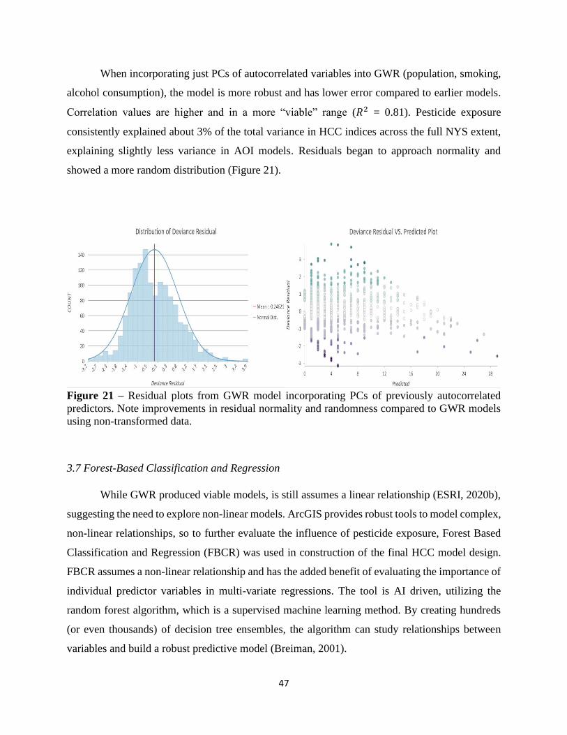
47

When incorporating just PCs of autocorrelated variables into GWR (population, smoking,

alcohol consumption), the model is more robust and has lower error compared to earlier models.

Correlation values are higher and in a more “viable” range (𝑅2 = 0.81). Pesticide exposure

consistently explained about 3% of the total variance in HCC indices across the full NYS extent,

explaining slightly less variance in AOI models. Residuals began to approach normality and

showed a more random distribution (Figure 21).

Figure 21 – Residual plots from GWR model incorporating PCs of previously autocorrelated

predictors. Note improvements in residual normality and randomness compared to GWR models

using non-transformed data.

3.7 Forest-Based Classification and Regression

While GWR produced viable models, is still assumes a linear relationship (ESRI, 2020b),

suggesting the need to explore non-linear models. ArcGIS provides robust tools to model complex,

non-linear relationships, so to further evaluate the influence of pesticide exposure, Forest Based

Classification and Regression (FBCR) was used in construction of the final HCC model design.

FBCR assumes a non-linear relationship and has the added benefit of evaluating the importance of

individual predictor variables in multi-variate regressions. The tool is AI driven, utilizing the

random forest algorithm, which is a supervised machine learning method. By creating hundreds

(or even thousands) of decision tree ensembles, the algorithm can study relationships between

variables and build a robust predictive model (Breiman, 2001).

48

FBCR models performed well, accurately predicting HCC counts per zip-code; however,

accuracy of count prediction is better in low count classes compared to high count classes (Figure

22). This disparity in count prediction accuracy between low and high-count classes persists from

previous models, though the levels of disagreement and general error are less severe. Most

importantly, FBCR models were consistent between runs, showed higher correlation values, and

over-all models were statistically significant.

Disagreement between the model and actual HCC counts (residuals) tend to occur around

populated areas. The model tends to over-predict in city centers, and under predict in suburban

areas, though this is not always the case. In most rural and wilderness areas, model-predicted HCC

counts are within 1 standard deviation (s.d.) of actual counts (Figure 23).

The 90% confidence prediction interval is tighter around lower HCC count classes,

widening above the mean. This indicates more uncertainty in higher count classes, though the

prediction interval is still relatively small and shows consistent width following a smooth curve.

The narrower prediction interval around zero count classes is likely due to the prevalence of zero-

count zip-codes. Overall, the prediction interval reflects a robust model. (Figure 24).

Removing zero-count classes from the model slightly reduces global correlation values

(𝑅2 = 0.78), likely due to reduced sample size. Otherwise there is not significant change in the

prediction interval, albeit the interval-curve becoming slightly less exponential (smoother) with

the interval narrower around one-count classes and expanding to a consistent width above the

mean, similar to previous FBCR models (Figure 25). In general, model robustness is not

significantly affected by removing zero-count zip-codes.

49

Figure 22 – Comparison of actual HCC counts to HCC counts predicted by Random Forest

model in NYS. Close match up between predicted and actual counts. Similar results in AOIs

with close match up between predicted and actual counts. Note how predicted counts are

especially close to actual counts around population centers, forming rings of HCC-density

(suburban areas tend to show the highest HCC counts).

50

Figure 23 – Residuals from FBCR model (difference between predicted HCC counts and actual

HCC counts). Note how most deviance occurs around population centers and how deviance is

low (within 1 s.d.) in mostly rural areas. Red areas indicate where the model is over-predicting

HCC counts, and blue areas indicate where the model is under-predicting HCC counts.

51

Figure 24 – 90% confidence prediction interval around each zip-code in NYS. Note widening of

interval in higher count classes.

Figure 25 – 90% confidence prediction interval around each zip-code in NYS using 10 validation

runs with 0 HCC count zip-codes removed. Note how the interval does not significantly change

from previous models, albeit a smoother curve and more consistent interval.

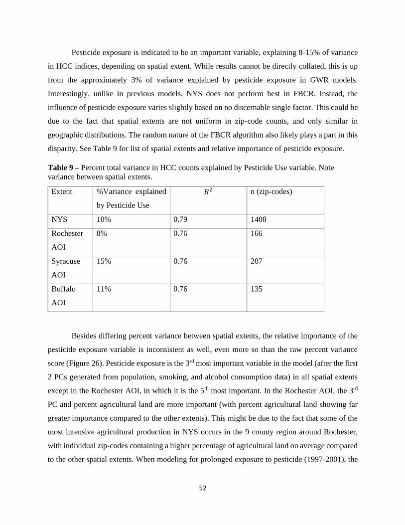
52

Pesticide exposure is indicated to be an important variable, explaining 8-15% of variance

in HCC indices, depending on spatial extent. While results cannot be directly collated, this is up

from the approximately 3% of variance explained by pesticide exposure in GWR models.

Interestingly, unlike in previous models, NYS does not perform best in FBCR. Instead, the

influence of pesticide exposure varies slightly based on no discernable single factor. This could be

due to the fact that spatial extents are not uniform in zip-code counts, and only similar in

geographic distributions. The random nature of the FBCR algorithm also likely plays a part in this

disparity. See Table 9 for list of spatial extents and relative importance of pesticide exposure.

Table 9 – Percent total variance in HCC counts explained by Pesticide Use variable. Note

variance between spatial extents.

Extent %Variance explained

by Pesticide Use

𝑅2 n (zip-codes)

NYS 10% 0.79 1408

Rochester

AOI

8% 0.76 166

Syracuse

AOI

15% 0.76 207

Buffalo

AOI

11% 0.76 135

Besides differing percent variance between spatial extents, the relative importance of the

pesticide exposure variable is inconsistent as well, even more so than the raw percent variance

score (Figure 26). Pesticide exposure is the 3rd most important variable in the model (after the first

2 PCs generated from population, smoking, and alcohol consumption data) in all spatial extents

except in the Rochester AOI, in which it is the 5th most important. In the Rochester AOI, the 3rd

PC and percent agricultural land are more important (with percent agricultural land showing far

greater importance compared to the other extents). This might be due to the fact that some of the

most intensive agricultural production in NYS occurs in the 9 county region around Rochester,

with individual zip-codes containing a higher percentage of agricultural land on average compared

to the other spatial extents. When modeling for prolonged exposure to pesticide (1997-2001), the

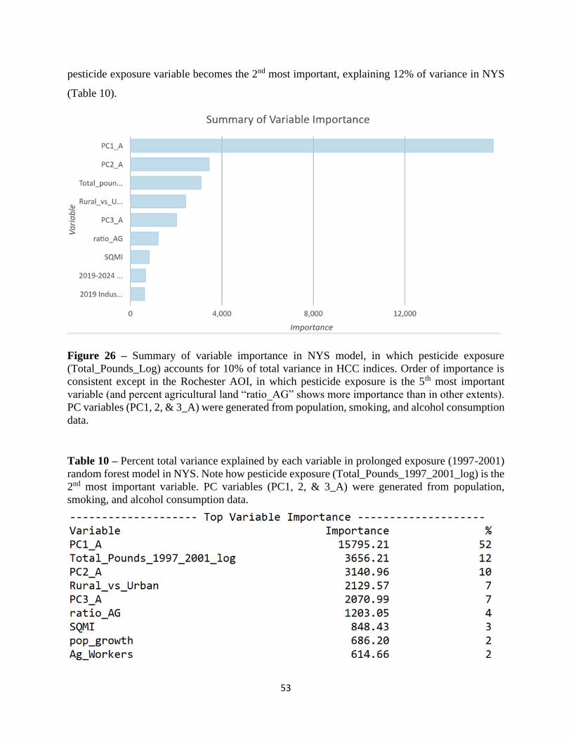
53

pesticide exposure variable becomes the 2nd most important, explaining 12% of variance in NYS

(Table 10).

Figure 26 – Summary of variable importance in NYS model, in which pesticide exposure

(Total_Pounds_Log) accounts for 10% of total variance in HCC indices. Order of importance is

consistent except in the Rochester AOI, in which pesticide exposure is the 5th most important

variable (and percent agricultural land “ratio_AG” shows more importance than in other extents).

PC variables (PC1, 2, & 3_A) were generated from population, smoking, and alcohol consumption

data.

Table 10 – Percent total variance explained by each variable in prolonged exposure (1997-2001)

random forest model in NYS. Note how pesticide exposure (Total_Pounds_1997_2001_log) is the

2nd most important variable. PC variables (PC1, 2, & 3_A) were generated from population,

smoking, and alcohol consumption data.

54

Models are statistically significant (p-value = 0.000 on validation data), show good out of

bag error (MSE = 4.354), with global correlation values on validation data ranging from 𝑅2 =

0.79 − 0.82, showing similar results to GWR correlation values. As found throughout model

design, global correlation values tend to be higher when modeling all NYS.

Increasing the number of validation runs performed by the model allows for variable

importance to be analyzed with more detail. The tool-generated summary of variance bar-chart

becomes a boxplot, showing the range of importance in each variable across the validation runs.

This allows for comparison between the importance of different variables to determine if they are

distinct from each other. When performing 10 validation runs, the pesticide exposure variable is

very close to the second principal component (of population, smoking, and alcohol consumption)

but is statistically distinct, separated by an importance score of 23 (Figure 27 & 28); however,

when performing 100 validation runs, the pesticide exposure variable is no longer distinct from

PC2, their maximum and minimum ranges overlapping (Figure 29 & 30). This indicates that while

pesticide exposure is considered an important variable, it cannot be said with certainty that it is

influencing higher HCC counts, or represents a real-world relationship. In general, all of the other

co-variates are relatively close to each other, with only the boxplot for PC1 (which explains 52%

of variance) showing a significant difference. It must be noted that as validation runs increase, the

spread of each variable boxplot increases as well. The model metrics (such as variance explained

(global 𝑅2 & individual variable), model out of bag errors, global statistical significance) show

little change between 10 and 100 validation runs.

55

Figure 27 – Distribution of variable importance on 10 validation runs. Note how the 1st principal

component of population, smoking, and alcohol consumption (PC1_A) is vastly more important

than the other variables, explaining 52% of the total variance. PC variables (PC1, 2, & 3_A) were

generated from population, smoking, and alcohol consumption data.

Figure 28 – Distribution of variable importance on 10 validation runs for principal component 2

of population, smoking, and alcohol consumption (PC2_A) and pesticide exposure

(Total_Pounds_Log). Note how importance distributions are remarkably close, but still distinct.

56

Figure 29 – Distribution of variable importance on 100 validation runs for PC2_A (principal

component 2 of population, smoking, and alcohol consumption) and pesticide exposure, in which

the importance distributions overlap considerably.

Figure 30 – Distribution of variable importance on 100 validation runs, in which PC1 is the only

statistically distinct variable, and all the other variables show overlap in importance distribution.

PC variables (PC1, 2, & 3_A) were generated from population, smoking, and alcohol

consumption data.

57

Predicted indices of HCC by a model not containing the pesticide exposure variable were

subtracted from predicted indices of HCC by the normal model containing the pesticide exposure

variable. This allowed for areas in-which pesticide exposure explains additional indices of HCC

to be highlighted. Zip-codes were divided into three classes based on the number of standard

deviations above or below mean predicted difference in HCC indices: Additional (> 1 s.d.), No

difference (± 1 s.d.), and Fewer (< 1 s.d.). See Figure 31 for geographic distribution of prediction

differences per zip-code, and Table 11 for counts of zip-codes in each class.

Figure 31 – Difference in predicted HCC indices based on pesticide exposure variable per zip-

code. Note areas of additional HCC indices predicted by pesticide exposure (highlighted in red).

Table 11 – Counts of zip-code in each HCC prediction class. Note how most zip-codes fall into

the “No Difference” class in which the pesticide exposure variable does not make a significant

difference on the number of predicted HCC indices.

Class Count

Additional 89

No Difference 1191

Fewer 107

58

Additional predicted HCC indices relating to the pesticide exposure variable occur mostly

in suburban and agricultural areas. The greatest additional indices predicted is 4 per zip-code in

Brighton, NY. Another notable region of additional HCC predicted by pesticide exposure is the

Finger Lakes. Zip-codes in which HCC indices prediction is greater than one standard deviation

above mean predicted indices is the smallest class. These results are evidence that the higher uses

of pesticide in these areas is related to these higher predicted indices of HCC. While in these areas

actual HCC counts are not above expected background, there is a trend from 2005 to 2015 in which

many of these areas show a shift from below expected observed HCC counts to normal observed

HCC counts (Figure 32).

Figure 32 – Deviation of observed HCC counts to expected HCC counts from 2005 to 2015. Note

increase in “normal” block-groups over time period (blue).

The vast majority of zip-codes fall in the “No Difference” range, in which the pesticide

exposure variable does not have a significant effect on predicted HCC indices (± 0.5 per zip-code).

These zip-codes largely fall in rural and wilderness areas.

59

Areas in which pesticide exposure predicts lower HCC indices are more randomly

dispersed, though they often are located in downtown areas/city centers. The greatest negative

indices predicted is 5 per zip-code in Niagara Falls, NY. Under-prediction zip-codes often follow

no discernable pattern and contradict with additional prediction areas, such as the Finger Lakes

region, which has a mix of additional and fewer class zip-codes (though additional HCC class zip-

codes are predominant). This suggests that additional variables are at play, such as indices of

hepatitis. Hepatitis was unable to be modeled reliably in this study due lack of IRB approval from

NYS DOH, restricting access to data at resolutions below the county level. Using the GIS

methodology developed are part of this study, future studies with access to zip-code level hepatitis

data and individual patient records will likely be able to construct models that predict actual HCC

counts with greater accuracy.

In general, most zip-codes show little difference between the models. Areas of additional

prediction occur often in suburban and agriculturally intensive areas. There seems to be a mix of

additional and fewer prediction classes, especially in suburban areas, with under prediction

occurring somewhat closer to city centers. This indicates that there is likely some metric that is

lacking in the model, which is driving these disparities. It could also be statistical artifacts from

the inherent randomness in the random forest model (ESRI, n.d.-d).

The FBCR model still displays issues of relatively high uncertainty and error overall. As

with previous model designs, removing the pesticide exposure variable does not actually have a

significant impact on the predictive power of the model, casting doubt as to whether the

“importance” of the relationship as measured by FBCR pertains to a real-world occurrence or is

an artifact of the statistical design. Explanatory variable range diagnostics indicate some error,

though there are no values so substantially out of range as to make the model statistically invalid.

When using the model to predict cancers not thought to be associated with pesticide

exposure, such as mesothelioma (which results from asbestos inhalation), correlation values on

validation data are much lower (𝑅2 = 0.37). This indicates that the model may indeed be detecting

a real association between pesticide exposure and HCC (See Table 12 and Appendix A1 & A2 for

model details).

60

3.8 Multi-Variate Cluster Analysis

While FBCR models performed generally well across the full dataset, results suggest that

there are unaccounted factors influencing the pesticide exposure-HCC relationship. This was

evident by the discrepancies in model performance, especially between different types of

geography. For example, FBCR models tend to perform best in rural areas, and deviate most from

actual HCC counts in more populated and developed areas. They also indicate great variance in

types of geography, land-use, and demographic makeup across the entirety of NYS. Even within

the defined AOIs, there is a complex mixture of land-uses, geographies, as well as large variance

in zip-code area and demographic and lifestyle factors. The complex relationships between these

variables were too complex to model (or control for lacking individual patient health information,

such as from the restricted NIH SEER-Medicare database) at the available data resolution (zip

codes) and with a single FBCR model.

In order to deal with the substantial variance across geographies, Multivariate Cluster

Analysis (MCA) was performed in ArcGIS. MCA generates clusters of geographies based on

specified parameters. MCA is a machine learning driven algorithm which finds an optimized

solution of sorting (clustering) between objects (in this case zip-code polygons with assigned

model attributes) by comparing every possible combination of features and outputs the resulting

combination with the best Calinski-Harabasz pseudo F-statistic (Caliński & Harabasz, 1974; ESRI,

n.d.-e). This tool allowed for the creation of specialized AOIs containing zip-codes that are similar

to each other along specified variables, such as population. Running FBCR on these specialized

AOIs created the ability to indirectly control for co-variates. For example, a model could be run

on a generated AOI consisting of zip-codes with similar levels of population, smoking, and alcohol

consumption.

MCA was performed across the full NYS dataset (with pesticide use and HCC outliers

removed). Initial clusters were based on all model variables. This generated two clusters, likely

based on the Urban vs. Rural classification Boolean variable. Indeed, the clusters seemed to follow

a geographic pattern along urban/rural lines; however, the clusters did not follow the true

urban/rural classification exactly, with some zip-codes that are clearly urban falling into the pseudo

“rural” cluster and vise-versa (Figure 33).

61

Figure 33 – Multivariate Cluster Analysis using all predictor variables. Note how clusters appear

to be largely based on the urban vs. rural Boolean classification variable.

FBCR tests were performed on these pseudo “urban” and “rural” clusters, using 100

validation runs with the original urban/rural variable removed to prevent data-redundancy in the

models. In general, models based on the “rural” cluster were more robust. This was expected, as

the greatest potential for pesticide exposure is in rural areas (VoPham et al., 2015), though it must

be noted that the “urban” cluster has a substantially smaller sample of zip-codes, which likely plays

a part in the differences in model performance (an issue which persisted in the MCA tests).

The FBCR model utilizing the “rural” cluster generally showed a greater prevalence of

higher HCC count class zip-codes. The prediction interval curve was steeper (more exponential)

compared to previous models, indicative of the higher prevalence of higher HCC count class zip-

codes (Figure 35). Pesticide exposure was shown to be important to the model (17% importance,

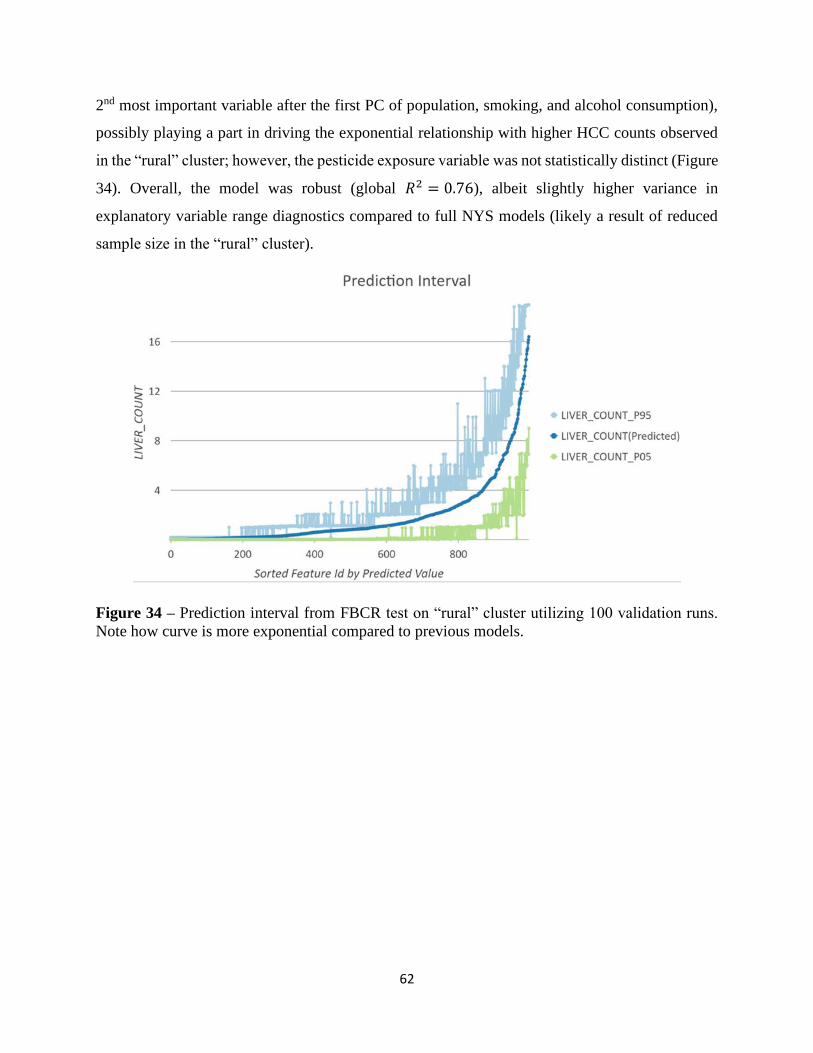
62

2nd most important variable after the first PC of population, smoking, and alcohol consumption),

possibly playing a part in driving the exponential relationship with higher HCC counts observed

in the “rural” cluster; however, the pesticide exposure variable was not statistically distinct (Figure

34). Overall, the model was robust (global 𝑅2 = 0.76), albeit slightly higher variance in

explanatory variable range diagnostics compared to full NYS models (likely a result of reduced

sample size in the “rural” cluster).

Figure 34 – Prediction interval from FBCR test on “rural” cluster utilizing 100 validation runs.

Note how curve is more exponential compared to previous models.

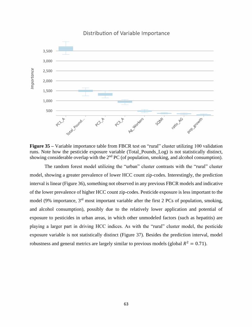
63

Figure 35 – Variable importance table from FBCR test on “rural” cluster utilizing 100 validation

runs. Note how the pesticide exposure variable (Total_Pounds_Log) is not statistically distinct,

showing considerable overlap with the 2nd PC (of population, smoking, and alcohol consumption).

The random forest model utilizing the “urban” cluster contrasts with the “rural” cluster

model, showing a greater prevalence of lower HCC count zip-codes. Interestingly, the prediction

interval is linear (Figure 36), something not observed in any previous FBCR models and indicative

of the lower prevalence of higher HCC count zip-codes. Pesticide exposure is less important to the

model (9% importance, 3rd most important variable after the first 2 PCs of population, smoking,

and alcohol consumption), possibly due to the relatively lower application and potential of

exposure to pesticides in urban areas, in which other unmodeled factors (such as hepatitis) are

playing a larger part in driving HCC indices. As with the “rural” cluster model, the pesticide

exposure variable is not statistically distinct (Figure 37). Besides the prediction interval, model

robustness and general metrics are largely similar to previous models (global 𝑅2 = 0.71).

64

Figure 36 – Prediction interval from random forest test on “urban” cluster, utilizing 100 validation

runs. Note the linear interval, in contrast to the exponential interval in previous models.

Figure 37 – Variable importance table from random forest test on “urban” cluster, utilizing 100

validation runs. Note how the pesticide exposure variable (Total_Pounds_Log) is less important

compared to the “rural” cluster model, and is not statistically distinct, showing considerable

overlap with the 3rd PC (of population, smoking, and alcohol consumption.

65

While initial MCA investigations showed interesting results, it was clear that the

relationships and variance between all the predictor variables was too great to generate meaningful

clusters, especially considering the overshadowing of other predictors by the urban/rural

classification. Therefore, MCA tests were performed on a subsets of original model predictors,

beginning with only the PC variables (PCs of population, smoking, and alcohol consumption).

This allowed for the generation of clusters in which zip-codes showed relative uniformity of these

demographic variables, enabling more confidence when ascertaining the influence of the pesticide

exposure variable.

Performing MCA along the PC variables produced 4 clusters, again seeming to mostly

follow geographic distributions, which is interesting considering the absence of the urban/rural

classification variable. Indeed, it seems that the geographic nature of a zip-code is strongly related

to its demographic and other co-variate makeup. This indicates that a raster surface approach might

be a good avenue for future analysis. As with the initial MCA, new pseudo “rural” and “urban”

clusters were produced, in addition to a new cluster seeming to follow a mostly “sub-urban”

distribution (these cluster will be referred to as rural2, urban2, and suburban). The 4th cluster

consisted of a single zip-code, which comprises the area surrounding Ithaca, NY (Figure 38). The

reasons as to why MCA could not group this zip-code with the other clusters is unclear. This zip-

code would continue to pop-up as an outlier in all following MCA, an issue which could be

addressed by future studies. For example, a future study could focus on MCA, building on the

methodology displayed here to create more optimized AOIs for a more controlled analysis.

FBCR tests were performed on these newly generated clusters, utilizing 100 validation runs

with the PC variables removed to prevent data-redundancy. Results were similar to previous MCA

tests in that the “rural2” cluster models were more robust compared to the “suburban” and

“urban2” clusters, which performed poorly, with pesticide exposure importance not statistically

distinct and very low global correlation (𝑅2 = 0.09). While this is an expected result in terms of

greatest potential for pesticide exposure, it must be noted that sample size is likely playing a large

part in model robustness as well, as the “rural2” cluster is significantly larger than the other

clusters.

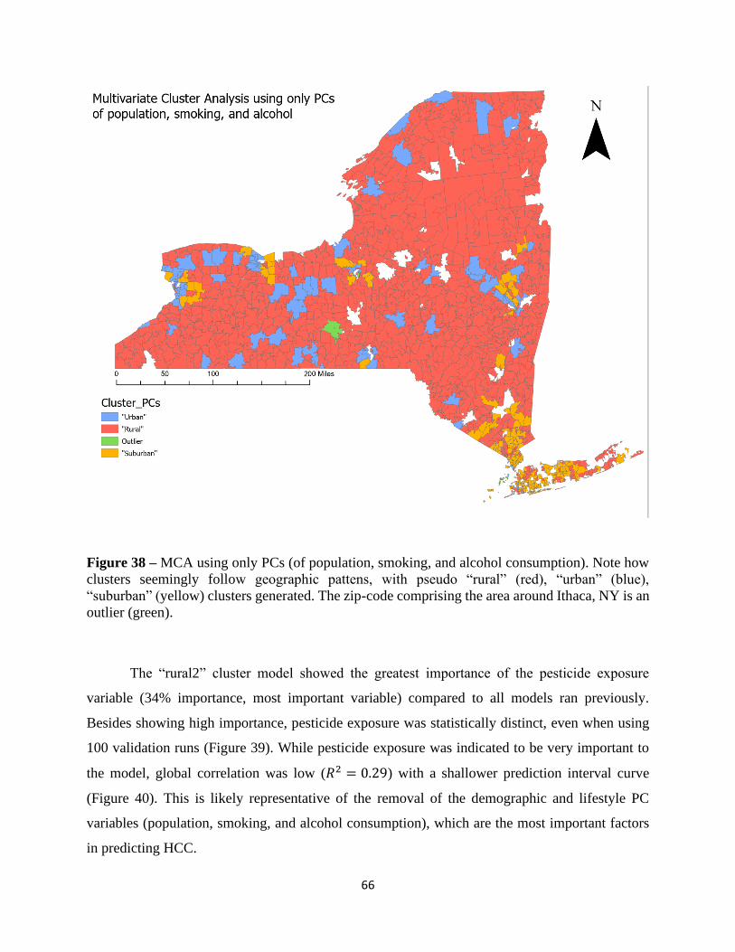
66

Figure 38 – MCA using only PCs (of population, smoking, and alcohol consumption). Note how

clusters seemingly follow geographic pattens, with pseudo “rural” (red), “urban” (blue),

“suburban” (yellow) clusters generated. The zip-code comprising the area around Ithaca, NY is an

outlier (green).

The “rural2” cluster model showed the greatest importance of the pesticide exposure

variable (34% importance, most important variable) compared to all models ran previously.

Besides showing high importance, pesticide exposure was statistically distinct, even when using

100 validation runs (Figure 39). While pesticide exposure was indicated to be very important to

the model, global correlation was low (𝑅2 = 0.29) with a shallower prediction interval curve

(Figure 40). This is likely representative of the removal of the demographic and lifestyle PC

variables (population, smoking, and alcohol consumption), which are the most important factors

in predicting HCC.

67

Figure 39 – Variable importance table from FBCR test performed on “rural2” cluster generated

from PCs of population, smoking, and alcohol consumption. FBCR performed across 100

validation runs. Note how pesticide exposure is the most important variable and statistically

distinct.

Figure 40 – Prediction interval from FBCR test performed on “rural2” cluster generated from PCs

of population, smoking, and alcohol consumption. FBCR performed across 100 validation runs.

Note how prediction interval curve is shallower (less exponential) compared to the FBCR test

performed on the original “rural2” cluster (based largely on urban/rural classification).

68

While pesticide exposure showed great importance, the overall model was weak. In order

to further investigate the influence of pesticide exposure using MCA and produce a robust FBCR

model, tests were again performed on the same clusters, this time using the original non-PCA

transformed model variables (non-transformed data of population, smoking, and alcohol

consumption). Additional MCA were performed utilizing PCs generated from the

demographic/lifestyle variables (population, smoking, and alcohol consumption) along with

pesticide exposure. FBCR tests were then performed on these new clusters using the original non-

PCA transformed variables.

MCA tests using the PCs (of pesticide exposure, population, smoking, and alcohol

consumption) followed similar trends to previous MCA, in that clusters appear to form across

geographic lines. With the inclusion of pesticide data into the PCs, more clusters were generated,

with a seemingly “wilderness” cluster forming, along with the usual rural, suburban, and urban

clusters (these clusters will be referred to as rural3, urban3, suburan2, and wilderness). As with

previous MCA, the zip-code comprising the area around Ithaca is an outlier (Figure 41). FBCR

tests performed on these final clusters did not produce as robust models as the clusters generated

from just the demographic/lifestyle PCs, which could be a result of reduced sample size due to the

greater number of clusters.

As with previous tests, the “rural3” cluster produced the most robust models, possibly a

factor of enhanced pesticide exposure in rural areas, as well the larger sample size available in the

rural cluster. When performing FBCR test using original, non-transformed model variables on the

initial PC based “rural2” cluster, pesticide exposure is the 4th most important variable (after

population, smoking, and alcohol consumption), with 8% importance. The pesticide exposure

variable was also statistically distinct, even when using 100 validation runs (Figure 42). This is

evidence that pesticide exposure may be playing a part in driving HCC indices, further back up by

the variable’s importance score and ranking, which is consistent with previous FBCR models.

69

Figure 41 – MCA using PCs of population, smoking, alcohol consumption, and pesticide

exposure. Note how clusters seemingly follow geographic patterns, with pseudo “urban” (yellow),

“suburban” (green), “rural” (blue), and “wilderness” (red) clusters being generated. The zip-code

comprising the area around Ithaca is an outlier (purple).

70

Figure 42 – Variable importance table from FBCR test performed on “rural” cluster (generated

from PCs of population, smoking, and alcohol consumption) using original non-transformed

variables over 100 validation runs. Note how pesticide exposure (Total_Pounds_Log) is the 4th

most importance variable and is statistically distinct.

71

Table 12 – Summary of general model types and results. Note: See A1 for summary of major model permutations and A2 for details

on specific model permutations.

Model Type Model Description R^2 Range R^2 Average n range (zip-codes) comments

GLR GLR 0.005 to 0.2 0.19 169 to 1576

Statistically significant but

weak relationships

OLS OLS

(-)0.0003 to

0.82 0.16 144 to 1576


weak relationships

ER ER 0.04 to 0.82 0.47 169 to 1576

Produced more robust models

than OLS and GLR, but still

limited by nature of purely

linear regressions

Agintense

Sub-analysis on

agriculturally intensive

zip-codes 0.87 to 0.91 0.89 19 to 147

Pesticide exposure indicated to

be a significant variable, but

overall models not significant

High HCC

Sub-analysis on high-

count HCC zip-codes 0.51 0.51 361

Models not as robust as models

utilizing full HCC dataset

LBR LBR 0 to 0.99 0.73 169 to 1576

Indicated clusters of positive

linear relationshps, benefits to

use of non-linear multi-variate

regressions

GWR GWR 0.33 to 0.9 0.58 169 to 1576

Better than linear models, but

the influence of pesticide

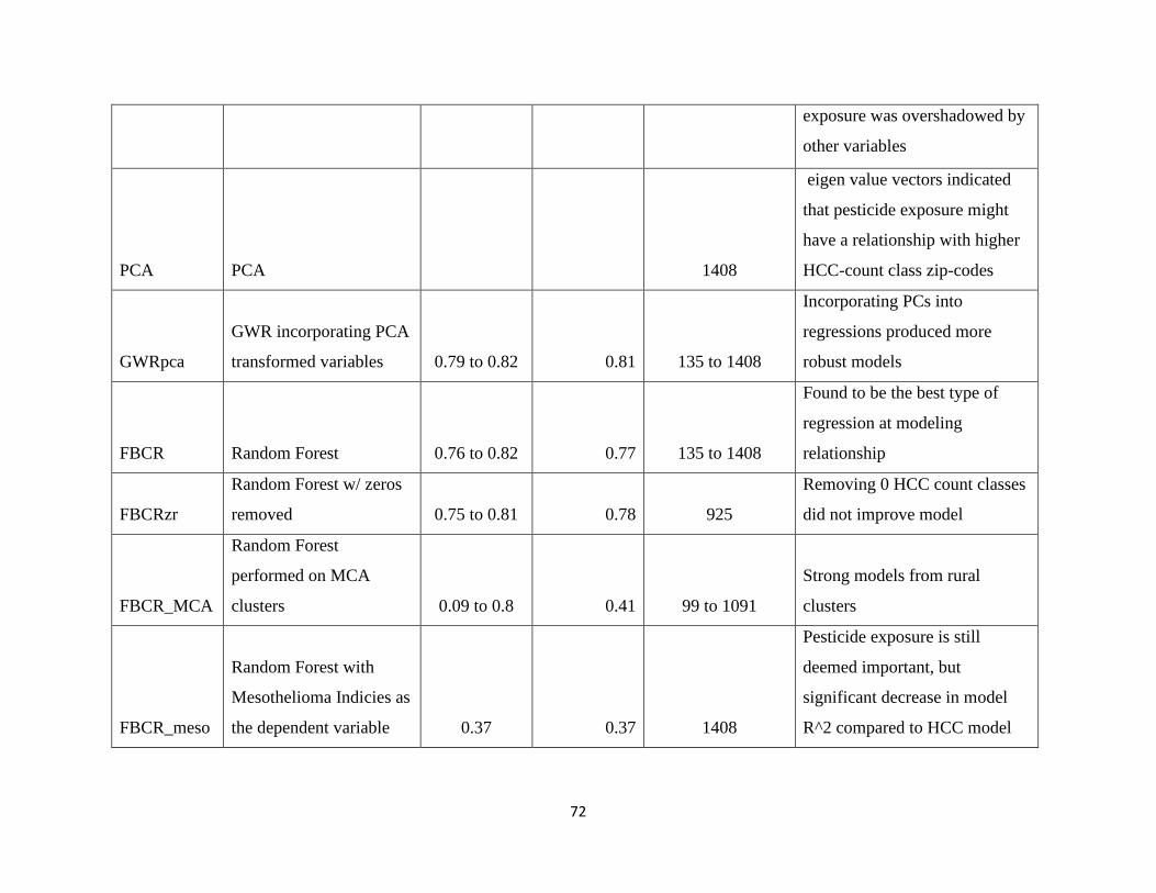
72

exposure was overshadowed by

other variables

PCA PCA

1408

eigen value vectors indicated

that pesticide exposure might

have a relationship with higher

HCC-count class zip-codes

GWRpca

GWR incorporating PCA

transformed variables 0.79 to 0.82 0.81 135 to 1408

Incorporating PCs into

regressions produced more

robust models

FBCR Random Forest 0.76 to 0.82 0.77 135 to 1408

Found to be the best type of

regression at modeling

relationship

FBCRzr

Random Forest w/ zeros

removed 0.75 to 0.81 0.78 925

Removing 0 HCC count classes

did not improve model

FBCR_MCA

Random Forest

performed on MCA

clusters 0.09 to 0.8 0.41 99 to 1091

Strong models from rural

clusters

FBCR_meso

Random Forest with

Mesothelioma Indicies as

the dependent variable 0.37 0.37 1408

Pesticide exposure is still

deemed important, but

significant decrease in model

R^2 compared to HCC model

73

4 General Discussion & Conclusion

The final FBCR models (NYS, AOIs, and Rural MCA cluster) showed a weak but

measurable positive relationship between pesticide exposure and HCC. It cannot be stated with

certainty that a statistically significant relationship has been observed, just that there is evidence

for a possible association.

This association began to manifest itself in the statistical data over the timeline of model

development described here. Beginning with simpler linear regression models, some statistically

significant relationships were observed. But overall models were weak, and results were highly

inconsistent. As analysis evolved into more complex non-linear and geographically weighted

models, the influence of pesticide exposure was detected with more consistency, but the signal

was weak and overshadowed by the many predictor variables. AI-driven non-linear regression,

principle component analysis, and cluster analysis-based models were ultimately able to measure

a significant relationship between pesticide exposure and HCC, while also maintaining a globally

significant and robust multi-variate regression.

While significant relationships were observed, the limitations of these stepwise,

investigative statistics must be noted. There is the immediate risk of creating models that are over-

fitted, generating statistics that while mathematically viable, may not actually represent a real-

world relationship. Therefore, there is controversy in the scientific community relating to the use

of such methods, with many flat out questioning the validity of this type of model development

(ESRI, n.d.-c). While an entire study could be devoted to describing the many intricacies of this

debate, it can be broken down generally into two main schools of scientific thought, the scientific

method viewpoint, and the data-miners viewpoint (ESRI, n.d.-c).

Strong proponents of the scientific method might reject the kinds of exploratory regression

used in this study. From their viewpoint, these methods run the risk of models that fit the data

being analyzed, but don’t actually reflect the true process playing out, creating, in other words, a

model which artificially fulfills a preconceived hypothesis. Furthermore, the many model

permutations and thousands of validation runs strongly increase the probability of type 1 error

(incorrectly rejecting the null-hypothesis, in this case that pesticide exposure and HCC are

unrelated).

74

On the other hand, researchers that follow the data-mining school of thought would feel

that it is impossible to know the right type of model and proper parameters before performing

investigative analysis when dealing with highly complex relationships. This is especially true when

there is no widely accepted established methodology or access to data is limited, as was the case

with this study. This data-mining school of thought is becoming more widely accepted as

computational power increases, with the ability to perform AI-driven multi-variate regressions

(Hand & Adams, 2015). In-fact, ESRI recommends such a path to using its statistical tool set,

suggesting a researcher beginning analysis using GLR models, as was done in this study (ESRI,

n.d.-d).

While an established methodology did exist from VoPham et al., (2015) for modeling the

pesticide exposure-HCC relationship in GIS, because of IRB restrictions, limited time, and the

overall scope of this study, it was not possible to fully emulate their methods. This is why a more

purely spatial, exploratory stepwise regression approach was used in order to develop viable final

models.

Vopham et al., (2015) were able to set up a case and control groups, aided by GIS

techniques (mostly to spatially link patient health-care records to zip-codes), due to the availability

of restricted individual patient records from the SEER-Medicare database. This allowed for a

detailed list of co-variates, such as age, pre-existing conditions, etc., to be linked to individuals

and directly controlled for. Only a subset of individuals that met lifestyle and pre-existing criteria

were included in the final case-control study. Furthermore, the individuals in this study were the

samples, providing much larger n-values than what could be done in the NYS models.

Additionally, California provides a larger geographic sample of zip-codes based on the states

larger size compared to NY (2597 to 1753; (Census Bureau, 2010)).

This study applied for but was denied IRB access to the SEER database, limiting the ability

to directly control for co-variates or create a true case-control study. But even if this restriction

didn’t exist, the data in NYS are somewhat self-limiting, as the database is not as expansive as the

datasets available in California. The SEER-Medicare database for NYS only has records dating

back to 1999, while California has records going back to the 1991 (National Cancer Institute,

2019).

75

Pesticide data is also much less robust in NYS. California has a state agency dedicated to

pesticide oversight, the California Department of Pesticide Regulation (CDPR) (CDPR 2020, n.d.).

This is in contrast to NYS, which tasks the DEC with pesticide use oversight. This results in

California having a pesticide dataset covering more year ranges, is at higher resolution, and has

more uniformity in reporting, including less error. There is more information on point-source

emissions of pesticides, in addition to time of application information, active ingredient chemical

information, and stricter guidelines on reporting that captures more sales and applications than

what are reported on in NYS.

Pesticide use records only go back to 1997 in NYS (NYS DEC, n.d.), while California has

records dating back to 1974. This difference in year ranges is significant, as this study was limited

to modeling cancer lags as long as 10 years with any reliability. Furthermore, NYS data are only

available at the zip-code resolution. California has pesticide applications recorded in much higher

resolution as part of the Public Land Survey System (PLSS), with data available at a square mile

resolution (specific 𝑚𝑖2 PLSS section where application took place (VoPham et al., 2015; CDPR

2020, n.d.). Besides higher resolution, this allows for geographic uniformity of pesticide

application samples, compared to the dis-jointed and highly irregular nature of zip-codes

geographies.

These database enhancements allowed Vopham et al. to create a pesticide exposure

variable based on use density (kg/mi2), directly controlling for area. Because the data in NYS are

based on zip-codes, creating such a density variable is fraught with more inherent error and does

not necessarily relate to a true distribution of pesticide use. This may be a reason as to why

pesticide exposure and area ultimately produced the best models while represented as individual

variables in a multi-variate regression.

California’s more robust pesticide dataset also aids in outlier analysis. CDPR puts out flag

levels for potential pesticide use outliers (a program which does not exist in NYS). This allowed

for Vopham et al., (2015) to perform a more targeted and accurate outlier analysis. This may be

part of the reason as to why VoPham et al., (2015) were able to observe statistically related

correlations between pesticide exposure and HCC.

The limitations of data in NYS forced this study to go along an almost pure geo-spatial

approach. Nonetheless, there has been little previous geo-spatial study of pesticide use in NYS,

76

besides hydrology-based studies, such as a GIS based contamination risk assessment of pesticide

ground-water contamination using run-off models(Ahirwar & Shukla, 2018). The data still yield

interesting results, many of which were in line with the California study. For example, in both

studies models performed weakest in urbanized areas. Ultimately, VoPham et al., (2015) only

found statistically significant correlations when modeling agriculturally intensive zip-codes in

isolation of other zones.

The subset analysis in NYS interestingly showed opposite results. Models on only

agriculturally intensive zip-codes were generally less robust, which could simply be due to the

lack of case-controlled individuals, and fewer zip-codes to sample compared to California. But

unlike observed in California, the best models in this study tended to encompass all of NYS.

Because a purely geo-spatial approach was taken, including exploratory regression modeling, it is

possible that the broader relationships at play were able to be more accurately analyzed than when

using a more traditional case-control study aided by GIS. In other words, because this study applied

GIS driven forest-based classification and regression to the HCC-pesticide exposure relationship,

something which has never been done before, it might be that the multi-variate regression system

developed here is detecting relationships which VoPham et al., (2015) could not with their more

standard case-control approach aided by GIS.

With improvements to model design in future studies, access to restricted data, and as

general quality of data increases, the tools used here may be able to more accurately represent the

HCC-pesticide exposure relationship. In general, few other pesticide epidemiology studies

utilizing spatial analysis have been done. Besides in California, a similar study was performed in

Crete, in which a higher prevalence of HCC was detected in regions of greater pesticide use

(Sifaki-Pistolla et al., 2015). Besides these studies, little has been done in the scientific community,

especially in the way this study has utilized complex models, such as random forest.

Besides highlighting evidence of an association between pesticide exposure and HCC, this

study applied new statistical methodologies not previously used on pre-existing datasets, creating

a framework from which future, more detailed analysis can be performed. This will become even

more pertinent as data itself improves in the future, along with the benefit of more years to model.

For example, NYSDEC has indicated that it wishes to improve the dataset. This includes unified

units in reporting, as currently reports are done in pounds and/or gallons, and not consistent,

77

sometimes reported as a mixture or active ingredient (NYSDEC Bureau of Pesticides

Management, 2013). With this study serving as a foundation, future studies can improve upon the

model design displayed here, incorporating more co-variates such as hepatitis indices, income

levels, and additional demographic information. With access to more individualized data, such as

IRB restricted individual patient information, much more robust models could potentially be

developed, including the development of case-control studies incorporating spatial information.

There are countless additional aspects of model design that could be experimented with, including

the incorporation of explanatory distance features, wind dispersal modeling, and converting data

to raster for surface-based analysis.

Even with the data-limitations mentioned above, this study found a statistically significant

impact from pesticide exposure on the distribution of HCC counts in models utilizing forest-based

classification and regression. This study is the first to use the random forest algorithm in this way,

allowing for the influence of pesticide exposure to be detected. This study therefore provides a

meaningful contribution to the scientific community, serving as a framework from which future

GIS-based study can be built. In addition, this study provides further evidence that there may be

health-risks related to pesticide exposure. As these risks are continued to be assessed, policy

makers can better develop regulations, and the populace at large can be made aware of potential

threats to their wellbeing.

78

References:

About the Data. (2018, July).

https://www.health.ny.gov/statistics/cancer/environmental_facilities/mapping/about/

Acquavella, J., Olsen, G., Cole, P., Ireland, B., Kaneene, J., Schuman, S., & Holden, L. (1998).

Cancer among Farmers: A Meta-Analysis. Annals of Epidemiology, 8(1), 64–74.

https://doi.org/10.1016/S1047-2797(97)00120-8

Ahirwar, S., & Shukla, J. P. (2018). Assessment of Groundwater Vulnerability in Upper Betwa

River Watershed using GIS based DRASTIC Model. Journal of the Geological Society of

India, 91(3), 334–340. https://doi.org/10.1007/s12594-018-0859-0

Alaa F. Badawi. (1999). Risk Factors for Hepatocellular Carcinoma in Egypt: The Role of

Hepatitis-B Viral Infection and Schistosomiasis. Anticancer Research, 19, 4563–4568.

Alavanja, M. C. R., & Bonner, M. R. (2012). Occupational Pesticide Exposures and Cancer

Risk: A Review. Journal of Toxicology and Environmental Health, Part B, 15(4), 238–

263. https://doi.org/10.1080/10937404.2012.632358

Alavanja, M. C. R., Dosemeci, M., Samanic, C., Lubin, J., Lynch, C. F., Knott, C., Barker, J.,

Hoppin, J. A., Sandler, D. P., Coble, J., Thomas, K., & Blair, A. (2004). Pesticides and

Lung Cancer Risk in the Agricultural Health Study Cohort. American Journal of

Epidemiology, 160(9), 876–885. https://doi.org/10.1093/aje/kwh290

Alavanja, M. C. R., & Hoppin, J. A. (2004). HEALTH EFFECTS OF CHRONIC PESTICIDE

EXPOSURE: Cancer and Neurotoxicity. Annual Review of Public Health, 25(1), 155–

197. https://doi.org/10.1146/annurev.publhealth.25.101802.123020

Alexander, D. D., Weed, D. L., Mink, P. J., & Mitchell, M. E. (2012). A weight-of-evidence

review of colorectal cancer in pesticide applicators: The agricultural health study and

other epidemiologic studies. International Archives of Occupational and Environmental

Health, 85(7), 715–745. https://doi.org/10.1007/s00420-011-0723-7

Amr, S., Dawson, R., Saleh, D. A., Magder, L. S., George, D. M. S., El-Daly, M., Squibb, K.,

Mikhail, N. N., Abdel-Hamid, M., Khaled, H., & Loffredo, C. A. (2013). Pesticides,

Gene Polymorphisms, and Bladder Cancer Among Egyptian Agricultural Workers.

Archives of Environmental & Occupational Health. http://www-tandfonline-

com.ezproxy.rit.edu/doi/abs/10.1080/19338244.2013.853646

79

ANSES. (2013, June 2). Exposure of the general population to pesticides | Anses—Agence

nationale de sécurité sanitaire de l’alimentation, de l’environnement et du travail.

ANSES - French Agency for Food, Environmental and Occupational Health & Safety.

https://www.anses.fr/en/content/exposure-general-population-pesticides

Anwar, W. A., Khaled, H. M., Amra, H. A., El-Nezami, H., & Loffredo, C. A. (2008). Changing

pattern of hepatocellular carcinoma (HCC) and its risk factors in Egypt: Possibilities for

prevention. Mutation Research, 659(1–2), 176–184.

https://doi.org/10.1016/j.mrrev.2008.01.005

APIPP. (2020). Adirondack Park Invasive Plant Program | About Us.

http://www.adkinvasives.com/About/About-Us/

Ashby, J., Brady, A., Elcombe, C. R., Elliott, B. M., Ishmael, J., Odum, J., Tugwood, J. D.,

Kettle, S., & Purchase, I. F. H. (1994). Mechanistically-based Human Hazard Assessment

of Peroxisome Proliferator-induced Hepatocarcinogenesis. Human & Experimental

Toxicology, 13(2 suppl), S1–S117. https://doi.org/10.1177/096032719401300201

Benbrook, C. M. (2012). Impacts of genetically engineered crops on pesticide use in the U.S. —

The first sixteen years. Environmental Sciences Europe, 24(1), 24.

https://doi.org/10.1186/2190-4715-24-24

Benbrook, C. M. (2016). Trends in glyphosate herbicide use in the United States and globally.

Environmental Sciences Europe, 28(1), 3. https://doi.org/10.1186/s12302-016-0070-0

Bender, D. A. (2006). Goitre. In Benders’ Dictionary of Nutrition and Food Technology (8th

ed.). Woodhead Publishing Ltd.

https://ezproxy.rit.edu/login?url=https://search.credoreference.com/content/entry/whdictn

utr/goitre/0?institutionId=3255

Bender, D. A. (2009). A Dictionary of Food and Nutrition. Oxford University Press.

Blair, A., & Zahm, S. (1991). Cancer among farmers. Occupational Medicine, 3, 335–354.

Blair, A., & Zahm, S. (1995). Agricultural exposures and cancer. Environmental Health

Perspectives, 103, 205–208.

Brandon Loomis. (2020, February 13). Adirondackers on guard against forest pests. Adirondack

Explorer. https://www.adirondackexplorer.org/stories/adirondackers-on-guard-against-

forest-pests

80

Breiman, L. (2001). Forest Based Classification and Regression. Machine Learning, 45(1), 5–32.

https://doi.org/10.1023/A:1010933404324

Brody, J. G., Aschengrau, A., McKelvey, W., Rudel, R. A., Swartz, C. H., & Kennedy, T.

(2004). Breast cancer risk and historical exposure to pesticides from wide-area

applications assessed with GIS. Environmental Health Perspectives, 112(8), 889–897.

Brooks, S. M., Stockwell, H. G., Pinkham, P. A., Armstrong, A. W., & Witter, D. A. (1992).

Sugarcane exposure and the risk of lung cancer and mesothelioma. Environmental

Research, 58(1), 195–203. https://doi.org/10.1016/S0013-9351(05)80215-4

Brun, G. L., MacDonald, R. M., Verge, J., & Aubé, J. (2008). Long-term atmospheric deposition

of current-use and banned pesticides in Atlantic Canada; 1980–2000. Chemosphere,

71(2), 314–327. https://doi.org/10.1016/j.chemosphere.2007.09.003

Caliński, T., & Harabasz, J. (1974). A dendrite method for cluster analysis. Communications in

Statistics, 3(1), 1–27. https://doi.org/10.1080/03610927408827101

Cancer Mapping Data: 2011-2015 | Health Data NY. (2018).

https://health.data.ny.gov/Health/Cancer-Mapping-Data-2011-2015/y4pv-ib8r

Carson, R. (1962). Silent Spring. Houghton Mifflin Harcourt.

Cattley, R. C., DeLuca, J., Elcombe, C., Fenner-Crisp, P., Lake, B. G., Marsman, D. S., Pastoor,

T. A., Popp, J. A., Robinson, D. E., Schwetz, B., Tugwood, J., & Wahli, W. (1998). Do

Peroxisome Proliferating Compounds Pose a Hepatocarcinogenic Hazard to Humans?

Regulatory Toxicology and Pharmacology, 27(1), 47–60.

https://doi.org/10.1006/rtph.1997.1163

CDC. (1999, October 1). Outbreak of West Nile-Like Viral Encephalitis—New York, 1999.

https://www.cdc.gov/mmwr/preview/mmwrhtml/mm4838a1.htm

CDPR 2020. (n.d.). California Department of Pesticide Regulation. Retrieved October 24, 2020,

from https://www.cdpr.ca.gov/

Census Bureau. (2010). United States Census Bureau 2010 report. Census.

http://www.census.gov/en.html

Chow, W.-H., Dong, L. M., & Devesa, S. S. (2010). Epidemiology and risk factors for kidney

cancer. Nature Reviews Urology, 7(5), 245–257. https://doi.org/10.1038/nrurol.2010.46

Cooke, B. K., & Stringer, A. (1982). Distribution and breakdown of DDT in orchard soil.

Pesticide Science, 13(5), 545–551. https://doi.org/10.1002/ps.2780130513

81

Cooper, G. M. (2000). Peroxisomes. https://www.ncbi.nlm.nih.gov/books/NBK9930/

Coupe, R. H., & Capel, P. D. (2016). Trends in pesticide use on soybean, corn and cotton since

the introduction of major genetically modified crops in the United States. Pest

Management Science, 72(5), 1013–1022. https://doi.org/10.1002/ps.4082

Damalas, C. A., & Eleftherohorinos, I. G. (2011). Pesticide Exposure, Safety Issues, and Risk

Assessment Indicators. International Journal of Environmental Research and Public

Health, 8(5), 1402–1419. https://doi.org/10.3390/ijerph8051402

Diamanti-Kandarakis, E., Bourguignon, J.-P., Giudice, L. C., Hauser, R., Prins, G. S., Soto, A.

M., Zoeller, R. T., & Gore, A. C. (2009). Endocrine-Disrupting Chemicals: An Endocrine

Society Scientific Statement. Endocrine Reviews, 30(4), 293–342.

https://doi.org/10.1210/er.2009-0002

Donna, A., Betta, P.-G., Robutti, F., Crosignani, P., Berrino, F., & Bellingeri, D. (1984). Ovarian

mesothelial tumors and herbicides: A case-control study. Carcinogenesis, 5(7), 941–942.

https://doi.org/10.1093/carcin/5.7.941

Dunnill, C. W., & Parkin, I. P. (2012). 9—Antimicrobial coatings for “self-sterilisation.” In

Sterilisation of Biomaterials and Medical Devices (pp. 240–260). Woodhead Publishing.

Dybing, E., Mikalesen, S., Huttunen, J., & Sanner, T. (1995). Peroxisome proliferation,

genotoxicity and carcinogenicity. http://www.julkari.fi/handle/10024/80962

Endocrine Disruptors. (2020, January 2). National Institute of Environmental Health Sciences.

https://www.niehs.nih.gov/health/topics/agents/endocrine/index.cfm

EPA. (2011). Summary of Results for the 2005 National Scale Assessment.

Eriksson, M., Hardell, L., Berg, N. O., Möller, T., & Axelson, O. (1981). Soft-tissue sarcomas

and exposure to chemical substances: A case-referent study. British Journal of Industrial

Medicine, 38(1), 27–33.

ESRI. (n.d.-a). Enrich Layer (Analysis)—ArcGIS Pro | Documentation. Retrieved October 25,

2020, from https://pro.arcgis.com/en/pro-app/tool-reference/analysis/enrich-layer.htm

ESRI. (n.d.-b). Exploratory Regression (Spatial Statistics)—ArcGIS Pro | Documentation.

Retrieved October 23, 2020, from https://pro.arcgis.com/en/pro-app/tool-

reference/spatial-statistics/exploratory-regression.htm

82

ESRI. (n.d.-c). How Exploratory Regression works—ArcGIS Pro | Documentation. Retrieved

October 24, 2020, from https://pro.arcgis.com/en/pro-app/tool-reference/spatial-

statistics/how-exploratory-regression-works.htm

ESRI. (n.d.-d). How Forest-Based Classification and Regression Works.

ESRI. (n.d.-e). How Multivariate Clustering works—ArcGIS Pro | Documentation. Retrieved

October 9, 2020, from https://pro.arcgis.com/en/pro-app/tool-reference/spatial-

statistics/how-multivariate-clustering-works.htm

ESRI. (n.d.-f). What they don’t tell you about regression analysis—ArcGIS Pro | Documentation.

Retrieved October 24, 2020, from https://pro.arcgis.com/en/pro-app/tool-

reference/spatial-statistics/what-they-don-t-tell-you-about-regression-analysis.htm

ESRI. (2020a). ArcGIS Pro | 2D and 3D GIS Mapping Software. https://www.esri.com/en-

us/arcgis/products/arcgis-pro/overview

ESRI. (2020b). Geographically Weighted Regression (GWR) (Spatial Statistics)—ArcGIS Pro |

Documentation. https://pro.arcgis.com/en/pro-app/tool-reference/spatial-

statistics/geographicallyweightedregression.htm

ESRI. (2020c). Local Bivariate Relationships (Spatial Statistics)—ArcGIS Pro | Documentation.

https://pro.arcgis.com/en/pro-app/tool-reference/spatial-

statistics/localbivariaterelationships.htm

ESRI. (2020d). Ordinary Least Squares (OLS) (Spatial Statistics)—ArcGIS Pro |

Documentation. https://pro.arcgis.com/en/pro-app/tool-reference/spatial-

statistics/ordinary-least-squares.htm

Ezzat, S., Abdel-Hamid, M., Abdel-Latif Eissa, S., Mokhtar, N., Albert Labib, N., El-Ghorory,

L., Nasmi Mikhail, N., Abdel-Hamid, A., Hifnawy, T., Thomas Strickland, G., &

Loffredo, C. A. (2005). Associations of pesticides, HCV, HBV, and hepatocellular

carcinoma in Egypt. International Journal of Hygiene and Environmental Health, 208(5),

329–339. https://doi.org/10.1016/j.ijheh.2005.04.003

Falck Jr., F., Ricci Jr., A., Wolff, M. S., Godbold, J., & Deckers, P. (1992). Pesticides and

Polychlorinated Biphenyl Residues in Human Breast Lipids and Their Relation to Breast

Cancer. Archives of Environmental Health, 47(2).

http://search.ebscohost.com/login.aspx?direct=true&db=afh&AN=5022562&site=ehost-

live

83

Falk, R. T., Pickle, L. W., Fontham, E. T., Correa, P., Morse, A., Chen, V., & Fraumeni, J. J.

(1990). Occupation and pancreatic cancer risk in Louisiana. American Journal of

Industrial Medicine, 18(5), 565–576. https://doi.org/10.1002/ajim.4700180507

Feitelson, M. A., Arzumanyan, A., Kulathinal, R. J., Blain, S. W., Holcombe, R. F., Mahajna, J.,

Marino, M., Martinez-Chantar, M. L., Nawroth, R., Sanchez-Garcia, I., Sharma, D.,

Saxena, N. K., Singh, N., Vlachostergios, P. J., Guo, S., Honoki, K., Fujii, H.,

Georgakilas, A. G., Bilsland, A., … Nowsheen, S. (2015). Sustained proliferation in

cancer: Mechanisms and novel therapeutic targets. Seminars in Cancer Biology, 35

Suppl, S25-54. https://doi.org/10.1016/j.semcancer.2015.02.006

Feng, Y., Liu, M., Chen, L., & Liu, Y. (2016). Simulation of Dynamic Urban Growth with

Partial Least Squares Regression-Based Cellular Automata in a GIS Environment. ISPRS

International Journal of Geo-Information, 5(12), 243.

https://doi.org/10.3390/ijgi5120243

Fernandez-Cornejo, J. (2009). First Decade of Genetically Engineered Crops in the United

States. DIANE Publishing.

Fernandez-Cornejo, J., Nehring, R. F., Osteen, C., Wechsler, S., Martin, A., & Vialou, A. (2014).

Pesticide Use in U.S. Agriculture: 21 Selected Crops, 1960-2008. SSRN Electronic

Journal. https://doi.org/10.2139/ssrn.2502986

Forastiere, F., Quercia, A., Miceli, M., Settimi, L., Terenzoni, B., Rapiti, E., Faustini, A., Borgia,

P., Cavariani, F., & Perucci, C. A. (1993). Cancer among farmers in central Italy.

Scandinavian Journal of Work, Environment & Health, 19(6), 382–389.

https://doi.org/10.5271/sjweh.1458

Friedrich, T. (2005). Does No-Till Farming Require More Herbicides? Outlooks on Pest

Management, 16(4), 188–191. https://doi.org/10.1564/16aug12

Friedrich, T., & Kassam, A. (2012). NO-TILL FARMING AND THE ENVIRONMENT: DO

NO-TILL SYSTEMS REQUIRE MORE CHEMICALS? Outlooks on Pest Management,

23(4), 153–157. https://doi.org/DOI:10.1564/23aug02

Furberg, A.-S., & Thune, I. (2003). Metabolic abnormalities (hypertension, hyperglycemia and

overweight), lifestyle (high energy intake and physical inactivity) and endometrial cancer

risk in a Norwegian cohort. International Journal of Cancer, 104(6), 669–676.

https://doi.org/10.1002/ijc.10974

84

Gomaa, A. I., Khan, S. A., Toledano, M. B., Waked, I., & Taylor-Robinson, S. D. (2008).

Hepatocellular carcinoma: Epidemiology, risk factors and pathogenesis. World Journal of

Gastroenterology : WJG, 14(27), 4300–4308. https://doi.org/10.3748/wjg.14.4300

Griffiths, A. J., Miller, J. H., Suzuki, D. T., Lewontin, R. C., & Gelbart, W. M. (2000).

Spontaneous mutations. https://www.ncbi.nlm.nih.gov/books/NBK21897/

Han, W., Yang, Z., Di, L., & Mueller, R. (2012). CropScape: A Web service based application

for exploring and disseminating US conterminous geospatial cropland data products for

decision support. Computers and Electronics in Agriculture, 84, 111–123.

https://doi.org/10.1016/j.compag.2012.03.005

Hand, D. J., & Adams, N. M. (2015). Data Mining. In Wiley StatsRef: Statistics Reference

Online (pp. 1–7). American Cancer Society.

https://doi.org/10.1002/9781118445112.stat06466.pub2

Hardell, L., & Sandström, A. (1979). Case-control study: Soft-tissue sarcomas and exposure to

phenoxyacetic acids or chlorophenols. British Journal of Cancer, 39(6), 711–717.

Hardell, Lennart, & Eriksson, M. (1988). The association between soft tissue sarcomas and

exposure to phenoxyacetic acids. A new case-referent study. Cancer, 62(3), 652–656.

https://doi.org/10.1002/1097-0142(19880801)62:3<652::AID-

CNCR2820620334>3.0.CO;2-4

Hellerstien, D., Vilorio, D., Ribaudo, M., Aillery, M., Bigelow, D., Bowman, M., Burns, C.,

Claassen, R., Crane-Droesch, A., Fooks, J., Greene, C., Hansen, L., Heisey, P., Hitaj, C.,

Hoppe, R., Key, N., Lynch, L., Malcom, S., Mcbride, W., … Wechsler, S. J. (2019).

USDA ERS - Agricultural Resources and Environmental Indicators, 2019.

https://www.ers.usda.gov/publications/pub-details/?pubid=93025

Hepatocellular carcinoma—Overview—Mayo Clinic. (2019, May 4).

https://www.mayoclinic.org/diseases-conditions/hepatocellular-carcinoma/cdc-20354552

Hu, J., Mao, Y., White, K., & The Canadian Cancer Registries Epidemiology Research Group.

(2002). Renal cell carcinoma and occupational exposure to chemicals in Canada. Society

of Occupational Medicine, 52(3), 157–164.

HUD USPS ZIP Code Crosswalk Files | HUD USER. (2019).

https://www.huduser.gov/portal/datasets/usps_crosswalk.html

85

IARC. (1991). Occupational Exposures in Insecticide Application, and Some Pesticides.

International Agency Research Cancer, 53, 535.

Jacobsen, S.-E., Sørensen, M., Pedersen, S. M., & Weiner, J. (2013). Feeding the world:

Genetically modified crops versus agricultural biodiversity. Agronomy for Sustainable

Development, 33(4), 651–662. https://doi.org/10.1007/s13593-013-0138-9

Jenner, P. (2001). Parkinson’s disease, pesticides and mitochondrial dysfunction. Trends in

Neurosciences, 24(5), 245–246. https://doi.org/10.1016/S0166-2236(00)01789-6

Kamel Boulos, M. N., Peng, G., & VoPham, T. (2019). An overview of GeoAI applications in

health and healthcare. International Journal of Health Geographics; London, 18.

http://dx.doi.org.ezproxy.rit.edu/10.1186/s12942-019-0171-2

Khuder, S. A., Mutgi, A. B., Schaub, E. A., & Tano, B. D. K. (1999). Meta-analysis of

Hodgkin’s disease among farmers. Scandinavian Journal of Work, Environment &

Health, 25(5), 436–441.

Kim, K.-H., Kabir, E., & Ara Jahan, S. (2016). Exposure to pesticides and associated human

health effects. Science of the Total Envrionment, 575(2017), 525–535.

Knower, K. C., To, S. Q., Leung, Y.-K., Ho, S.-M., & Clyne, C. D. (2014). Endocrine disruption

of the epigenome: A breast cancer link. Endocrine-Related Cancer, 21(2), T33–T55.

https://doi.org/10.1530/ERC-13-0513

Koutros, S., Silverman, D. T., Alavanja, M. C., Andreotti, G., Lerro, C. C., Heltshe, S., Lynch,

C. F., Sandler, D. P., Blair, A., Freeman, B., & E, L. (2016). Occupational exposure to

pesticides and bladder cancer risk. International Journal of Epidemiology, 45(3), 792–

805. https://doi.org/10.1093/ije/dyv195

Kuwata, K., Inoue, K., Ichimura, R., Takahashi, M., Kodama, Y., Shibutani, M., & Yoshida, M.

(2017). β-catenin Mutations Are Not Involved in Early-stage Hepatocarcinogenesis

Induced by Protoporphyrinogen Oxidase Inhibitors in Mice. Toxicologic Pathology,

45(4), 493–505. https://doi.org/10.1177/0192623317708898

Ledda, C., Loreto, C., Zammit, C., Marconi, A., Fago, L., Matera, S., Costanzo, V., Fuccio

Sanzà, G., Palmucci, S., Ferrante, M., Costa, C., Fenga, C., Biondi, A., Pomara, C., &

Rapisarda, V. (2017). Non‑infective occupational risk factors for hepatocellular

carcinoma: A review (Review). Molecular Medicine Reports, 15(2), 511–533.

https://doi.org/10.3892/mmr.2016.6046

86

Lee, D.-H., Lind, P. M., Jacobs, D. R., Salihovic, S., van Bavel, B., & Lind, L. (2016).

Association between background exposure to organochlorine pesticides and the risk of

cognitive impairment: A prospective study that accounts for weight change. Environment

International, 89–90, 179–184. https://doi.org/10.1016/j.envint.2016.02.001

Lee, S. F., Huang, Y. T., Wu, W. S., & Lin, J. K. (1996). Induction of c-jun protooncogene

expression by hydrogen peroxide through hydroxyl radical generation and p60SRC

tyrosine kinase activation. Free Radical Biology and Medicine, 21(4), 437–448.

https://doi.org/10.1016/0891-5849(96)00040-8

Lee, W. J., Lijinsky, W., Heineman, E. F., Markin, R. S., Weisenburger, D. D., & Ward, M. H.

(2004). Agricultural pesticide use and adenocarcinomas of the stomach and oesophagus.

Occupational and Environmental Medicine, 61(9), 743–749.

https://doi.org/10.1136/oem.2003.011858

Lehman, H. (1993). New Directions for Pesticide Use. In D. Pimentel & H. Lehman (Eds.), The

Pesticide Question (pp. 3–9). Springer US. https://doi.org/10.1007/978-0-585-36973-0_1

Lehmann, J. M., Moore, L. B., Smith-Oliver, T. A., Wilkison, W. O., Willson, T. M., & Kliewer,

S. A. (1995). An Antidiabetic Thiazolidinedione Is a High Affinity Ligand for

Peroxisome Proliferator-activated Receptor γ (PPARγ). Journal of Biological Chemistry,

270(22), 12953–12956. https://doi.org/10.1074/jbc.270.22.12953

Lerro, C. C., Koutros, S., Andreotti, G., Friesen, M. C., Alavanja, M. C., Blair, A., Hoppin, J. A.,

Sandler, D. P., Lubin, J. H., Ma, X., Zhang, Y., & Freeman, L. E. B. (2015).

Organophosphate insecticide use and cancer incidence among spouses of pesticide

applicators in the Agricultural Health Study. Occupational and Environmental Medicine,

72(10), 736–744. https://doi.org/10.1136/oemed-2014-102798

Longley, P. A., & Batty, M. (1996). Spatial Analysis: Modelling in a GIS Environment. John

Wiley & Sons.

Lynge, E. (1985). A follow-up study of cancer incidence among workers in manufacture of

phenoxy herbicides in Denmark. British Journal of Cancer, 52(2), 259–270.

Mabuchi, K., Lilienfeld, A. M., & Snell, L. M. (1979). Lung Cancer among Pesticide Workers

Exposed to Inorganic Arsenicals. Archives of Environmental Health, 34(5).

http://search.ebscohost.com/login.aspx?direct=true&db=hch&AN=5020165&site=ehost-

live

87

Mabuchi, K., Lilienfeld, A. M., & Snell, L. M. (1980). Cancer and occupational exposure to

arsenic: A study of pesticide workers. Preventive Medicine, 9(1), 51–77.

https://doi.org/10.1016/0091-7435(80)90059-6

Maitra, S., & Yan, J. (2008). Principle Component Analysis and Partial Least Squares: Two

Dimension Reduction Techniques for Regression. 12.

Marrs, T. C., & Ballantyne, B. (Eds.). (2004). Pesticide toxicology and international regulation.

J. Wiley.

Mathers, J. C., Strathdee, G., & Relton, C. L. (2010). 1—Induction of Epigenetic Alterations by

Dietary and Other Environmental Factors. In Z. Herceg & T. Ushijima (Eds.), Advances

in Genetics (Vol. 71, pp. 3–39). Academic Press. https://doi.org/10.1016/B978-0-12-

380864-6.00001-8

Matisova, E., & Hrouzkov, S. (2012). Endocrine disrupting pesticides. In R. P. Soundararajan

(Ed.), Pesticides—Advances in Chemical and Botanical Pesticides. InTech.

https://doi.org/10.5772/46226

McGlynn, K. A., Quraishi, S. M., Graubard, B. I., Weber, J.-P., Rubertone, M. V., & Erickson,

R. L. (2008). Persistent Organochlorine Pesticides and Risk of Testicular Germ Cell

Tumors. JNCI: Journal of the National Cancer Institute, 100(9), 663–671.

https://doi.org/10.1093/jnci/djn101

Mena, S., Ortega, A., & Estreka, J. M. (2008). Oxidative stress in enviornmental-induced

carcinogenesis. Mutation Research, 674(2009), 36–44.

Nanni, O., Amadori, D., Lugaresi, C., Falcini, F., Scarpi, E., Saragoni, A., & Buiatti, E. (1996).

Chronic lymphocytic leukaemias and non-Hodgkin’s lymphomas by histological type in

farming-animal breeding workers: A population case-control study based on a priori

exposure matrices. Occupational and Environmental Medicine, 53(10), 652–657.

National Cancer Institute. (2019, November 8). Paranasal Sinus and Nasal Cavity Cancer

Treatment (Adult) (PDQ®)–Patient Version [PdqCancerInfoSummary]. National Cancer

Institute. https://www.cancer.gov/types/head-and-neck/patient/adult/paranasal-sinus-

treatment-pdq

Niu, J., Lin, Y., Guo, Z., Niu, M., & Su, C. (2016). The Epidemiological Investigation on the

Risk Factors of Hepatocellular Carcinoma. Medicine, 95(6).

https://doi.org/10.1097/MD.0000000000002758

88

NYS DEC. (n.d.). Pesticide Annual Report Data—NYS Dept. Of Environmental Conservation.

Retrieved August 21, 2017, from http://www.dec.ny.gov/chemical/96898.html

NYS DOH. (2019, December). About the Institutional Review Board (IRB)).

https://www.health.ny.gov/professionals/irb/

NYSDEC. (2017). Pesticide Annual Report Data—NYS Dept. Of Environmental Conservation.

Department of Environmental Conservation.

http://www.dec.ny.gov/chemical/96898.html

NYSDEC Bureau of Pesticides Management. (2013). PRL Annual Reports—NYS Dept. Of

Environmental Conservation. https://www.dec.ny.gov/chemical/97535.html

NYSDOH. (2013, January). Environmental Facilities and Cancer Mapping.

https://www.health.ny.gov/statistics/cancer/environmental_facilities/mapping/

Orr, S. (2016, August 26). Watchdog: Suburban lawns drive huge pesticide use in Monroe.

Rochester Democrat and Chronicle.

http://www.democratandchronicle.com/story/news/2016/08/26/pesticide-usage-monroe-

county/88764456/

Owens, K., Feldman, J., & Kepner, J. (2010). Wide range of diseases linked to pesticides. Pestic.

You, 30, 13–21.

Perry, E. D., Ciliberto, F., Hennessy, D. A., & Moschini, G. (2016). Genetically engineered

crops and pesticide use in U.S. maize and soybeans. Science Advances, 2(8), e1600850.

https://doi.org/10.1126/sciadv.1600850

Persson, E. C., Graubard, B. I., Evans, A. A., London, W. T., Weber, J.-P., LeBlanc, A., Chen,

G., Lin, W., & McGlynn, K. A. (2012). Dichlorodiphenyltrichloroethane and risk of

hepatocellular carcinoma. International Journal of Cancer, 131(9), 2078–2084.


Pesticide Sales and Use Reporting. (2017). http://psur.cce.cornell.edu/

Polanco Rodríguez, Á. G., Riba López, M. I., DelValls Casillas, T. Á., Araujo León, J. A.,

Mahjoub, O., & Prusty, A. K. (2017). Monitoring of organochlorine pesticides in blood

of women with uterine cervix cancer. Environmental Pollution, 220, 853–862.

https://doi.org/10.1016/j.envpol.2016.10.068

Purdue, M. P., Hoppin, J. A., Blair, A., Dosemeci, M., & Alavanja, M. C. R. (2007).

Occupational exposure to organochlorine insecticides and cancer incidence in the

89

Agricultural Health Study. International Journal of Cancer, 120(3), 642–649.


Rakitsky, V. N., Koblyakov, V. A., & Turusov, V. S. (2000). Nongenotoxic (epigenetic)

carcinogens: Pesticides as an example. A critical review. Teratogenesis, Carcinogenesis,

and Mutagenesis, 20(4), 229–240. https://doi.org/10.1002/1520-

6866(2000)20:4<229::AID-TCM5>3.0.CO;2-M

Rau, A. T. K., Coutinho, A., Shreedhara Avabratha, K., Rau, A. R., & Warrier, R. P. (2012).

Pesticide (Endosulfan) levels in the bone marrow of children with hematological

malignancies. Indian Pediatrics, 49(2), 113–117. https://doi.org/10.1007/s13312-012-

0025-5

Shen, S., Lin, Y., Yuan, X., Shen, L., Chen, J., Chen, L., Qin, L., & Shen, B. (2016). Biomarker

MicroRNAs for Diagnosis, Prognosis and Treatment of Hepatocellular Carcinoma: A

Functional Survey and Comparison. Scientific Reports, 6.

https://doi.org/10.1038/srep38311

Shim Youn K., Mlynarek Steven P., & van Wijngaarden Edwin. (2009). Parental Exposure to

Pesticides and Childhood Brain Cancer: U.S. Atlantic Coast Childhood Brain Cancer

Study. Environmental Health Perspectives, 117(6), 1002–1006.

https://doi.org/10.1289/ehp.0800209

Shmaefsky, B. R. (2013). Agricultural Biotechnology: History, Science, and Society. Choice;

Middletown, 51(2), 199-202,204-208.

Siddiqui, M. K. J., & Saxena, M. C. (1985). Placenta and Milk as Excretory Routes of Lipophilic

Pesticides in Women. Human Toxicology, 4(3), 249–254.

https://doi.org/10.1177/096032718500400304

Sifaki-Pistolla, D., Karageorgos, S., Koulentaki, M., D, S., Stratakou, S., E, D., & Kouroumalis,

E. (2015). Geoepidemiology of Hepatocellular Carcinoma in the island of Crete, Greece.

A possible role of pesticides. Liver International.

Silke, J., & Meier, P. (2013). Inhibitor of Apoptosis (IAP) Proteins–Modulators of Cell Death

and Inflammation. Cold Spring Harbor Perspectives in Biology, 5(2).

https://doi.org/10.1101/cshperspect.a008730

Snow, J. (1855). On the Mode of Communication of Cholera. John Churchill.

90

Steuer, C. E., El‐Deiry, M., Parks, J. R., Higgins, K. A., & Saba, N. F. (2017). An update on

larynx cancer. CA: A Cancer Journal for Clinicians, 67(1), 31–50.

https://doi.org/10.3322/caac.21386

Stokes, L., Stark, A., Marshall, E., & Narang, A. (1995). Neurotoxicity among pesticide

applicators exposed to organophosphates. Occupational and Environmental Medicine,

52(10), 648–653.

Street, J. C., & Sharma, R. P. (1975). Alteration of induced cellular and humoral immune

responses by pesticides and chemicals of environmental concern: Quantitative studies of

immunosuppression by DDT, aroclor 1254, carbaryl, carbofuran, and methylparathion.

Toxicology and Applied Pharmacology, 32(3), 587–602. https://doi.org/10.1016/0041-

008X(75)90123-4

Tapestry. (n.d.). Retrieved March 3, 2020, from https://www.esri.com/en-

us/arcgis/products/tapestry-segmentation/overview

The R Foundation. (2020). Prcomp function | R Documentation.

https://www.rdocumentation.org/packages/stats/versions/3.6.2/topics/prcomp

Tom Koch. (2005). Cartographies of Disease. ESRI Press.

Tu, J. (2011). Spatially varying relationships between land use and water quality across an

urbanization gradient explored by geographically weighted regression. Applied

Geography, 31(1), 376–392. https://doi.org/10.1016/j.apgeog.2010.08.001

Turusov, V., Rakitsky, V., & Revazova, Y. (1998). Once again on the problem of threshold in

chemical carcinogenesis. Vopr. Oncology, 44, 468–476.

United Nations. (2001). Pesticide Residues in Food, 2001: Report of the Joint Meeting of the

FAO Panel of Experts on Pesticide Residues in Food and the Environment and the WHO

Core Assessment Group on Pesticide Residues. Food & Agriculture Org.

Vais, H., Williamson, M. S., Devonshire, A. L., & Usherwood, P. N. R. (2001). The molecular

interactions of pyrethroid insecticides with insect and mammalian sodium channels. Pest

Management Science, 57(10), 877–888. https://doi.org/10.1002/ps.392

Vettorazzi, G., Almeida, W. F., Burin, G. J., Jaeger, R. B., Puga, F. R., Rahde, A. F., Reyes, F.

G., & Schvartsman, S. (1995). International safety assessment of pesticides:

Dithiocarbamate pesticides, ETU, and PTU—A review and update. Teratogenesis,

91

Carcinogenesis, and Mutagenesis, 15(6), 313–337.

https://doi.org/10.1002/tcm.1770150608

Vineis, P., Terracini, B., Ciccone, G., Cignetti, A., Colombo, E., Donna, A., Maffi, L., Pisa, R.,

Ricci, P., Zanini, E., & Comba, P. (1987). Phenoxy herbicides and soft-tissue sarcomas in

female rice weeders: A population-based case-referent study. Scandinavian Journal of

Work, Environment & Health, 13(1), 9–17.

VoPham, T., Brooks, M. M., Yuan, J.-M., Talbott, E. O., Ruddell, D., Hart, J. E., Chang, C.-C.

H., & Weissfeld, J. L. (2015). Pesticide exposure and hepatocellular carcinoma risk: A

case-control study using a geographic information system (GIS) to link SEER-Medicare

and California pesticide data. Environmental Research, 143, Part A, 68–82.

https://doi.org/10.1016/j.envres.2015.09.027

Waddell, B. L., Zahm, S. H., Baris, D., Weisenburger, D. D., Holmes, F., Burmeister, L. F.,

Cantor, K. P., & Blair, A. (2001). Agricultural use of organophosphate pesticides and the

risk of non-Hodgkin’s lymphoma among male farmers (United States). Cancer Causes &

Control, 12(6), 509–517. https://doi.org/10.1023/A:1011293208949

Wang, H.-S., Zhao, Y.-G., Man, Y.-B., Wong, C. K. C., & Wong, M.-H. (2011). Oral

bioaccessibility and human risk assessment of organochlorine pesticides (OCPs) via fish

consumption, using an in vitro gastrointestinal model. Food Chemistry, 127(4), 1673–

1679. https://doi.org/10.1016/j.foodchem.2011.02.035

Weichenthal Scott, Moase Connie, & Chan Peter. (2010). A Review of Pesticide Exposure and

Cancer Incidence in the Agricultural Health Study Cohort. Environmental Health

Perspectives, 118(8), 1117–1125. https://doi.org/10.1289/ehp.0901731

Whitford, F., Acquavella, J., & Burns, C. (2003). PESTICIDES AND EPIDEMIOLOGY

Unraveling Disease Patterns. Purdue Pesticide Programs.

Wilson, R., & Din, Alexander. (2020). Understanding and Enhancing the U.S. Department of

Housing and Urban Development’s ZIP Code Crosswalk Files. Cityscape: A Journal of

Policy Development and Research, 22(1), 18.

Wingren, G., Fredrikson, M., Brage, H. N., Nordenskjöld, B., & Axelson, O. (1990). Soft tissue

sarcoma and occupational exposures. Cancer, 66(4), 806–811.

https://doi.org/10.1002/1097-0142(19900815)66:4<806::AID-

CNCR2820660435>3.0.CO;2-U

92

Xu, X., Tao, Y., Niu, Y., Wang, Z., Zhang, C., Yu, Y., & Ma, L. (2019). MiR-125a-5p inhibits

tumorigenesis in hepatocellular carcinoma. Aging (Albany NY), 11(18), 7639–7662.

https://doi.org/10.18632/aging.102276

Yildirim, M., Kaya, V., Yildiz, M., Demirpence, O., Gunduz, S., & Dilli, U. D. (2014).

Esophageal Cancer, Gastric Cancer and the use of Pesticides in the Southwestern of

Turkey. Asian Pacific Journal of Cancer Prevention, 15(6), 2821–2823.

https://doi.org/10.7314/APJCP.2014.15.6.2821

93

Appendix:

A1 – Summary of model types and results. Note: See A2 for details on specific model permutations.

Model Type Model Type Spatial Extent R^2 Range

R^2

Average

n (zip-

codes) comments

GLR GLR NYS 0.006 to 0.2 0.08 1576


weak relationships

GLR R GLR Rochester AOI 0.005 to 0.15 0.3 169


weak relationships

OLS OLS NYS 0.006 to 0.82 0.49 1576


weak relationships

OLS R OLS Rochester AOI 0.06 to 0.8 0.35 169


weak relationships

OLS OR

OLS with all outliers

removed NYS 0.02 0.02 953


weak relationships

OLS R OR


removed Rochester AOI 0.23 0.23 144


weak relationships

OLS Rate

OLS using HCC rates

as dependent variable NYS -0.0003 -0.0003 1576

OLS (and other models) are

less viable when modeling for

HCC rates

OLS Rate OR

OLS using HCC rates

as dependent variable

with all outliers

removed NYS 0.002 0.002 953



HCC rates

OLS Rate R OR

OLS using HCC rates

as dependent variable

with all outliers

removed Rochester AOI -0.006 -0.006 144



HCC rates

OLS NYCR

OLS with Greater

NYC Area removed NYS 0.07 to 0.29 0.18 1115

Removing the greater NYC

area did not improve model

performance

ER ER NYS 0.04 to 0.82 0.57 1576



94


linear regressions

ER R ER Rochester AOI 0.07 to 0.8 0.36 169




linear regressions

Agintense 1

Sub-analysis on

agriculturally

intensive zip-codes NYS 0.91 0.91 19

Pesticide exposure not

indicated to be a significant

variable, high error

Agintense 2

Sub-analysis on

agriculturally

intensive zip-codes NYS 0.87 0.87 147

Pesticide exposure indicated to

be a significant variable, but

overall models not significant

High HCC

Sub-analysis on high-

count HCC zip-codes NYS 0.51 0.51 361

Models not as robust as

models utilizing full HCC

dataset

LBR LBR NYS 0 to 0.99 0.57 1576


linear relationships, benefits to


regressions

LBR R LBR Rochester AOI 0.89 0.89 169


linear relationships, benefits to


regressions

GWR GWR NYS 0.6 to 0.9 0.7 1576



exposure was overshadowed

by other variables

GWR R GWR Rochester AOI 0.33 to 0.8 0.45 169



exposure was overshadowed

by other variables

PCA PCA NYS 1408

eigen value vectors indicated

that pesticide exposure might

have a relationship with higher

HCC-count class zip-codes

95

GWRpca

GWR incorporating

PCA transformed

variables NYS 0.81 0.81 1408



robust models

GWRpca R

GWR incorporating

PCA transformed

variables Rochester AOI 0.8 0.08 166



robust models

GWRpca S

GWR incorporating

PCA transformed

variables Syracuse AOI 0.82 0.82 207



robust models

GWRpca B

GWR incorporating

PCA transformed

variables Buffalo AOI 0.79 0.79 135



robust models

FBCR Random Forest NYS 0.79 to 0.82 0.8 1408



relationship

FBCR R Random Forest Rochester AOI 0.76 0.76 166



relationship

FBCR S Random Forest Syracuse AOI 0.76 0.76 207



relationship

FBCR B Random Forest Buffalo AOI 0.76 0.76 135



relationship

FBCRzr

Random Forest w/

zeros removed NYS 0.75 to 0.81 0.78 925



relationship

FBCR_MCAr

Random Forest

performed on MCA

clusters Rural AOI 0.76 0.76 992

Strong models from rural

clusters

FBCR_MCAu

Random Forest

performed on MCA

clusters Urban AOI 0.71 0.71 408

Weaker models from urban,

suburban, & wilderness

clusters

FBCR_MCA2r

Random Forest

performed on MCA

clusters Rural2 AOI 0.29 to 0.8 0.55 1091



clusters

96

FBCR_MCA2u

Random Forest

performed on MCA

clusters Urban2 AOI 0.09 0.09 117



clusters

FBCR_MCAs

Random Forest

performed on MCA

clusters Suburban AOI 0.09 0.09 177



clusters

FBCR_MCA3r

Random Forest

performed on MCA

clusters Rural3 AOI 0.75 0.75 757



clusters

FBCR_MCA3u

Random Forest

performed on MCA

clusters Urban3 AOI 0.05 0.05 99



clusters

FBCR_MCAw

Random Forest

performed on MCA

clusters Wilderness AOI 0.6 0.6 406



clusters

FBCR_MCA2s

Random Forest

performed on MCA

clusters Suburban2 AOI 0.08 0.08 130



clusters

FBCR_meso

Random Forest with

Mesothelioma Indicies

as the dependent

variable NYS 0.37 0.37 1408

Pesticide exposure is still

deemed important, but

significant decrease in model

R^2 compared to HCC model

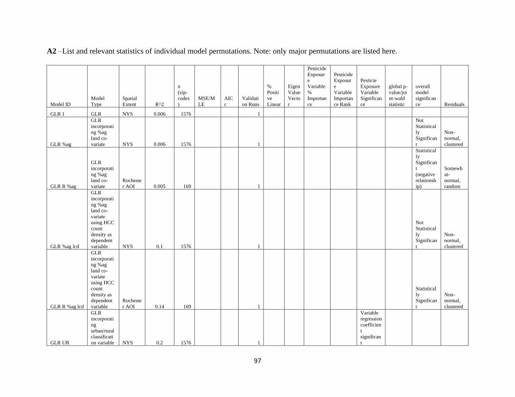
97

A2 –List and relevant statistics of individual model permutations. Note: only major permutations are listed here.

Model ID

Model

Type

Spatial

Extent R^2

n

(zip-codes

)

MSE/M

LE

AIC

c

Validati

on Runs

%

Positive

Linear

Eigen

Value Vecto

r

Pesticide

Exposure

Variable

% Importan

ce

Pesticide Exposur

e

Variable Importan

ce Rank

Pesticie

Exposure

Variable Significan

ce

global p-

value/joint-wald

statistic

overall

model significan

ce Residuals

GLR 1 GLR NYS 0.006 1576 1

GLR %ag

GLR

incorporating %ag

land co-

variate NYS 0.006 1576 1

Not

Statistically

Significan

t

Non-

normal,

clustered

GLR R %ag

GLR incorporati

ng %ag

land co-variate

Rochester AOI 0.005 169 1

Statistical

ly

Significant

(negative

relationship)

Somewh

at-

normal, random

GLR %ag lcd

GLR

incorporati

ng %ag

land co-

variate using HCC

count

density as dependent

variable NYS 0.1 1576 1

Not

Statistical

ly Significan

t

Non-normal,

clustered

GLR R %ag lcd

GLR

incorporating %ag

land co-

variate using HCC

count

density as

dependent

variable

Rocheste

r AOI 0.14 169 1

Statistical

ly

Significan

t

Non-

normal,

clustered

GLR UR

GLR incorporati

ng

urban/rural classificati

on variable NYS 0.2 1576 1

Variable regression

coefficien

t significan

t

98

GLR R UR

GLR incorporati

ng


on variable

Rocheste

r AOI 0.15 169 1

Variable regresion

coefficien

t not significan

t

OLS 1 OLS NYS 0.006 1576

13172 1

Variable

regression coefficien

t

significant 5.58

Not Statistical

ly

Significant

Non-

normal, clustered

OLS 1R OLS Rochester AOI 0.06 169 1128 1

Variable


t

significant 11.73

Not Statistical

ly

Significant

Non-

normal, clustered

OLS 1Ra OLS

Rocheste

r AOI 0.07 169 999 1

Variable

regression

coefficient

significan

t 3.18

Not

Statistically

Significan

t

Non-

normal,

clustered

OLS 1a OLS NYS 0.006 1576

1311

1 1

Variable

regresion

coefficien

t not

significan

t 7.41

Not

Statistical

ly

Significan

t

Non-

normal,

clustered

OLS OR

OLS with

all outliers

removed NYS 0.02 953

1283

0 1

Variable

regression

coefficient

significan

t 31.26

Not

Statistically

Significan

t

Non-

normal,

clustered

OLS R OR


removed

Rocheste

r AOI 0.23 144 807 1

Variable regression

coefficien

t significan

t 49.87

Not

Statistical

ly Significan

t

Somewhat-

normal,

somewhat-

clustered

OLS Rate

OLS using

HCC rates

as dependent

variable NYS -0.0003 1576

-2295

3 1

Variable regresion

coefficien

t not significan

t 3.17

Not

Statistical

ly Significan

t

Non-normal,

clustered

99

OLS Rate OR

OLS using HCC rates

as

dependent variable

with all

outliers removed NYS 0.002 953

-

24867 1

Variable


t

significant 8.65

Not Statistical

ly

Significant

Non-

normal, clustered

OLS Rate R

OR

OLS using

HCC rates

as dependent

variable

with all outliers

removed

Rocheste

r AOI -0.006 144

-

2329 1

Variable regresion

coefficien

t not significan

t 0.41

Not

Statistical

ly Significan

t

Somewh

at-normal,

patterned

OLS NYCR

OLS with

Greater NYC Area

removed NYS 0.07 1115 6897 1

Variable regression

coefficien

t significan

t 6.22

Not

Statistical

ly Significan

t

Non-normal,

clustered

OLS NYCR popd

OLS with

Greater NYC Area

removed, using

population

density co-variate NYS 0.29 1115 6684 1

Variable


t

significant 62.38

Not Statistical

ly

Significant

Somewh

at-

normal, patterned

OLS pd

OLS with

pesticide

density as "pesticide

exposure"

variable NYS 0.09 1576 3809 1

Variable

regresion

coefficient not

significan

t 9.35

Not

Statistically

Significan

t

Non-

normal,

clustered

OLS R pd

OLS with

pesticide

density as "pesticide

exposure"

variable

Rocheste

r AOI 0.42 169 779 1

Variable

regression

coefficient

significan

t 33.06

Not

Statistically

Significan

t

Somewh

at-

normal, somewha

t-

clustered

OLS %ag

OLS

incorporating %ag

land co-

variate NYS 0.63 1576 864 1

Variable regression

coefficien

t significan

t

(negative) 88.21

Not

Statistically

Significan

t

Somewh

at-

normal, somewha

t-

clustered

100

OLS %ag pr

OLS incorporati

ng %ag

land co-variate

with

pesticide exposure

variable

removed NYS 0.61 1576 868 1

Somewhat-

normal,

clustered

OLS %ag lcd

OLS incorporati

ng %ag

land co-variate

using HCC

count density as

dependent

variable NYS 0.39 1576

1200

7 1

Variable

regression

coefficient

significan

t 216

Not

Statistically

Significan

t

Somewh

at-

normal, somewha

t-

clustered

OLS %ag lcd

pr

OLS

incorporati

ng %ag land co-

variate

using HCC count

density as

dependent variable

with

pesticide exposure

variable


1202

1 1 211

Not

Statistically

Significan

t

Somewh

at-

normal, somewha

t-

clustered

OLS %ag R lcd

OLS

incorporati

ng %ag land co-

variate

using HCC count

density as

dependent variable

Rochester AOI 0.14 169 684 1

Variable

regresion coefficien

t not

significant 16.47

Not Statistical

ly

Significant

Non-

normal, clustered

OLS %ag R lcd

pr

OLS

incorporati

ng %ag land co-

variate

Rocheste

r AOI 0.14 169 682 1 16.46

Not

Statistical

ly Significan

t

Non-normal,

clustered

101

using HCC count

density as

dependent variable

with

pesticide exposure

variable

removed

OLS 2

OLS using

enriched

co-variates NYS 0.82 1576

1040

2 1

Variable regression

coefficien

t significan

t

(negative) 1871

Not

Statistically

Significan

t

Somewh

at-normal,

somewha

t-random

OLS 2 pr

OLS using

all enriched

co-variates with

pesticide

exposure variable


1043

4 1 1395

Not

Statistical

ly Significan

t

Somewh

at-

normal, somewha

t-random

OLS 2 R

OLS using all enriched

co-variates

Rocheste

r AOI 0.8 169 777 1

Variable regresion

coefficien

t not significan

t 395

Not

Statistical

ly Significan

t

Somewh

at-

normal, somewha

t-random

OLS UR

OLS incorporati

ng


on variable NYS 0.82 1576

1042

3 1

Variable


t

significant

(negative) 1471

Not

Statistical

ly Significan

t

Somewh

at-normal,

clustered

OLS UR pr

OLS incorporati

ng

urban/rural

classificati

on variable

with pesticide

exposure

variable removed NYS 0.82 1576

10436 1 1440

Not Statistical

ly

Significant

Somewh

at-

normal, clustered

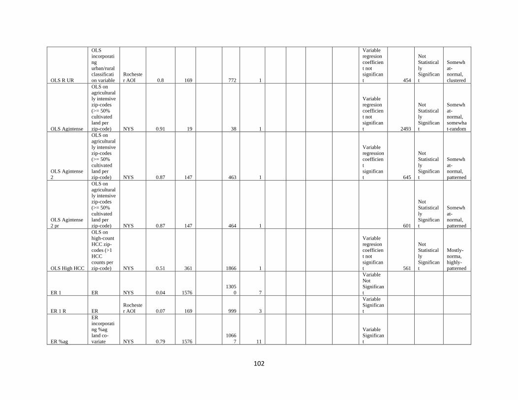
102

OLS R UR

OLS incorporati

ng


on variable

Rocheste

r AOI 0.8 169 772 1

Variable regresion

coefficien

t not significan

t 454

Not

Statistical

ly Significan

t

Somewh

at-normal,

clustered

OLS Agintense

OLS on


zip-codes

(>= 50% cultivated

land per

zip-code) NYS 0.91 19 38 1

Variable

regresion

coefficient not

significan

t 2493

Not

Statistically

Significan

t

Somewh

at-normal,

somewha

t-random

OLS Agintense

2

OLS on

agricultural

ly intensive zip-codes

(>= 50%

cultivated land per

zip-code) NYS 0.87 147 463 1

Variable regression

coefficien

t significan

t 645

Not

Statistical

ly Significan

t

Somewh

at-normal,

patterned

OLS Agintense 2 pr

OLS on


zip-codes (>= 50%

cultivated

land per zip-code) NYS 0.87 147 464 1 601

Not Statistical

ly

Significant

Somewh

at-

normal, patterned

OLS High HCC

OLS on

high-count

HCC zip-codes (>1

HCC

counts per zip-code) NYS 0.51 361 1866 1

Variable

regresion coefficien

t not

significant 561

Not Statistical

ly

Significant

Mostly-

norma,

highly-patterned

ER 1 ER NYS 0.04 1576

1305

0 7

Variable

Not Significan

t

ER 1 R ER Rochester AOI 0.07 169 999 3

Variable

Significant

ER %ag

ER

incorporating %ag

land co-

variate NYS 0.79 1576

1066

7 11

Variable

Significan

t

103

ER %ag R

ER incorporati

ng %ag

land co-variate


Variable

Significant

ER %ag lcd

ER

incorporati

ng %ag land co-

variate

using HCC count

density as

dependent variable NYS 0.38 1576

12022 4

Variable

Not

Significant

ER %ag R lcd

ER

incorporating %ag

land co-

variate using HCC

count

density as dependent

variable

Rocheste

r AOI 0.05 169 695 2

Variable

Not Significan

t

ER 2

ER using all enriched

co-variates NYS 0.82 1576

1040

2 8

Variable Significan

t

ER 2 R

ER using all enriched

co-variates

Rocheste

r AOI 0.8 169 777 8

Variable

Not Significan

t

ER UR

ER incorporati

ng


on variable NYS 0.82 1576

1042

3 9

Variable Significan

t

ER R UR

ER

incorporating

urban/rural

classification variable


Variable

Not

Significant

ER Agintense

ER on


zip-codes

(>= 50% cultivated NYS 0.91 19 38 7

Variable

Not

Significant

104

land per zip-code)

ER Agintense 2

ER on

agricultural

ly intensive zip-codes

(>= 50%

cultivated land per

zip-code) NYS 0.87 147 463 8

Variable Significan

t

ER High HCC

ER on high-count

HCC zip-

codes (>1 HCC

counts per

zip-code) NYS 0.51 361 1868 9

LBR 1 LBR NYS 0.9 (best zip-code) 1576 1 30

LBR density

LBR using

HCC and pesticide

pounds

normalized to area NYS

0.95 (best zip-code) 1576 1 14

LBR %ag HCC

LBR

between

%ag and

HCC

counts NYS

No

significan

t

relationsh

ips 1576 1 0

LBR 2

LBR using log

transforme

d pesticide exposure NYS

0.99 (best zip-code) 1576 1

LBR 2 R

LBR using

log transforme

d pesticide

exposure

Rocheste

r AOI

0.89 (best

zip-code) 169 1

LBR UR

LBR

between

HCC

counts and urban/rural

classificati

on NYS

No

significant

relationsh

ips 1576 1

GWR 1 GWR NYS 0.6 1576 264

1142

6 1

Somewh

at-

105

normal, patterned

GWR 1R GWR

Rocheste

r AOI 0.33 169 51 878 1

Non-

normal,

clustered

GWR 1a GWR NYS 0.62 1576 45 1

GWR

Agworkers

GWR using

number of

agricultural workers as

explanator

y variable NYS 0.66 1576 258 9386 1

Non-

normal,

clustered

GWR R Agworkers

GWR

using

number of agricultural

workers as

explanatory variable

Rochester AOI 0.33 169 46 708 1

Non-

normal, clustered

GWR 2

GWR

incorporati

ng enriched variables NYS 0.9 1576 255 3106 1

Somewh

at-

normal, patterned

GWR R 2

GWR

incorporating enriched

variables

Rocheste

r AOI 0.8 169 44 243 1

Somewh

at-normal,

patterned

GWR HCC P

GWR with only

pesticide

exposure (log base e

transforme

d) as explanator

y variable NYS 0.62 1576 261

1062

6 1

Somewh

at-normal,

patterned

GWR lcd

GWR

using HCC count

density as

dependent variable NYS 0.64 1576 65

11185 1

Somewh

at-

normal, patterned

GWR lcd R

GWR

using HCC count

density as

dependent variable

Rochester AOI 0.35 169 4 643 1

Somewh

at-

normal, patterned

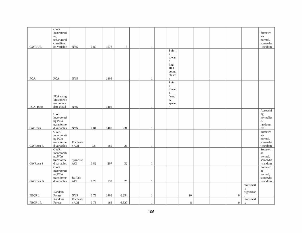
106

GWR UR

GWR incorporati

ng


on variable NYS 0.89 1576 3 1

Somewh

at-

normal, somewha

t-random

PCA PCA NYS 1408 1

Point

s towar

d

high HCC

count

cluster

PCA_meso

PCA using Mesothelio

ma counts

data cloud NYS 1408 1

Point

s towar

d

"empty

space

"

GWRpca

GWR

incorporating PCA

transforme

d variables NYS 0.81 1408 231 1

Aproaching

normality &

randomn

ess

GWRpca R

GWR incorporati

ng PCA

transformed variables


Somewhat-

normal,

somewhat-random

GWRpca S

GWR

incorporating PCA

transforme

d variables

Syracuse

AOI 0.82 207 32 1

Somewh

at-normal,

somewha

t-random

GWRpca B

GWR incorporati

ng PCA


Buffalo AOI 0.79 135 25 1

Somewhat-

normal,

somewhat-random

FBCR 1

Random

Forest NYS 0.79 1408 6.354 1 10 0

Statistical

ly Significan

t

FBCR 1R

Random

Forest

Rocheste

r AOI 0.76 166 6.327 1 8 0

Statistical

ly

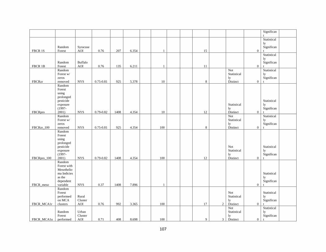
107

Significant

FBCR 1S Random Forest

Syracuse AOI 0.76 207 6.354 1 15 0

Statistical

ly

Significant

FBCR 1B

Random

Forest

Buffalo

AOI 0.76 135 6.211 1 11 0

Statistical

ly Significan

t

FBCRzr

Random

Forest w/ zeros

removed NYS 0.75-0.81 925 5.378 10 8

Not

Statistically

Distinct 0

Statistical

ly Significan

t

FBCRpro

Random Forest

using

prolonged pesticide

exposure

(1997-2001) NYS 0.79-0.82 1408 4.354 10 12

Statistical

ly Distinct 0

Statistical

ly

Significant

FBCRzr_100

Random

Forest w/

zeros removed NYS 0.75-0.81 925 4.354 100 8

Not

Statistical

ly Distinct 0

Statistical

ly

Significant

FBCRpro_100

Random

Forest using

prolonged

pesticide exposure

(1997-

2001) NYS 0.79-0.82 1408 4.354 100 12

Not Statistical

ly

Distinct 0

Statistically

Significan

t

FBCR_meso

Random

Forest with

Mesothelioma Indicies

as the

dependent variable NYS 0.37 1408 7.896 1 0

Statistical

ly

Significant

FBCR_MCA1r

Random

Forest

performed on MCA

clusters

Rural Cluster

AOI 0.76 992 3.365 100 17 2

Not

Statistically

Distinct 0

Statistical

ly Significan

t

FBCR_MCA1u

Random

Forest

performed

Urban

Cluster

AOI 0.71 408 8.698 100 9 3

Not Statistical

ly

Distinct 0

Statistically

Significan

t

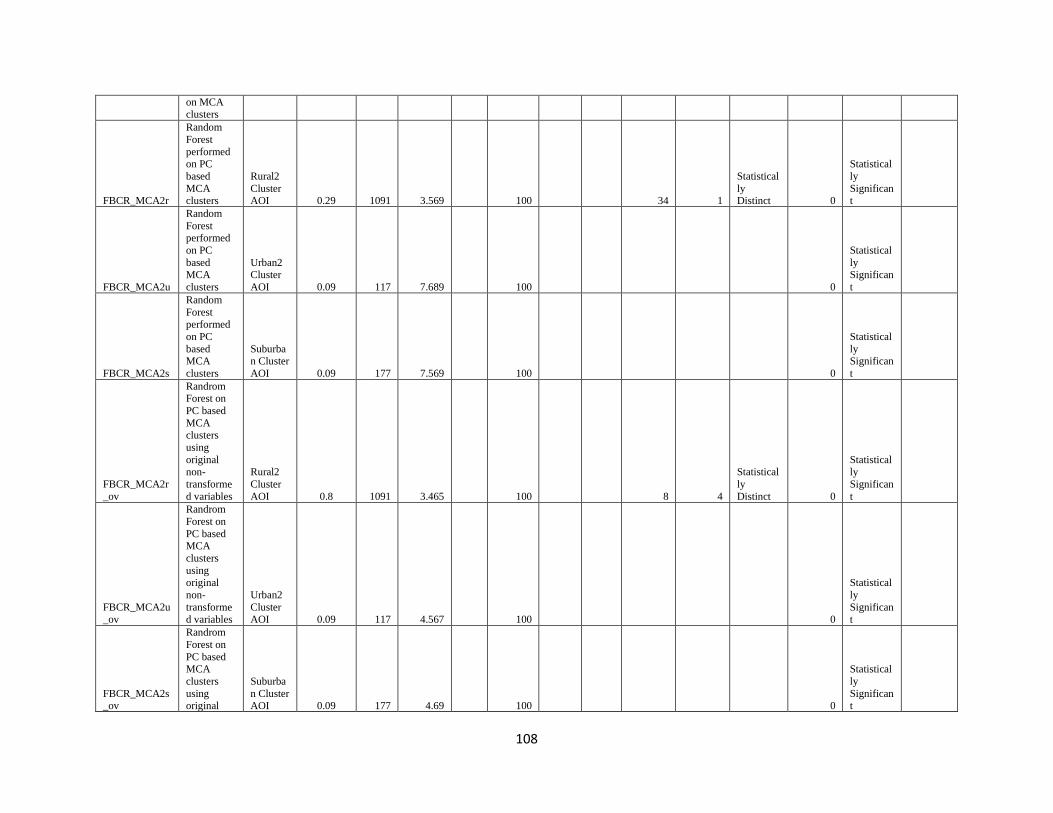
108

on MCA clusters

FBCR_MCA2r

Random

Forest

performed on PC

based

MCA clusters

Rural2

Cluster AOI 0.29 1091 3.569 100 34 1

Statistical

ly Distinct 0

Statistical

ly

Significant

FBCR_MCA2u

Random

Forest performed

on PC

based MCA

clusters

Urban2 Cluster

AOI 0.09 117 7.689 100 0

Statistical

ly Significan

t

FBCR_MCA2s

Random

Forest performed

on PC

based MCA

clusters

Suburban Cluster

AOI 0.09 177 7.569 100 0

Statistical

ly Significan

t

FBCR_MCA2r

_ov

Randrom Forest on

PC based

MCA

clusters

using

original non-

transforme

d variables

Rural2

Cluster

AOI 0.8 1091 3.465 100 8 4

Statistical

ly

Distinct 0

Statistically

Significan

t

FBCR_MCA2u

_ov

Randrom

Forest on

PC based MCA

clusters

using original

non-

transforme

d variables

Urban2

Cluster

AOI 0.09 117 4.567 100 0

Statistical

ly

Significan

t

FBCR_MCA2s_ov

Randrom

Forest on

PC based MCA

clusters

using original

Suburba

n Cluster AOI 0.09 177 4.69 100 0

Statistical

ly

Significant

109

non-transforme

d variables

FBCR_MCA3r

Random

Forest on PC

(including

pesticide exposure)

based

MCA clusters

using

original non-

transforme

d variables

Rural3

Cluster

AOI 0.75 757 3.969 100 0

Statistically

Significan

t

FBCR_MCA3

w

Random

Forest on

PC (including

pesticide

exposure) based

MCA

clusters using

original

non-transforme

d variables

Wildern

ess AOI 0.6 406 7.898 100 0

Statistical

ly Significan

t

FBCR_MCA3s

Random Forest on

PC

(including pesticide

exposure)

based MCA

clusters

using original

non-


Suburba

n2

Cluster AOI 0.08 130 8.544 100 0

Statistical

ly

Significant

FBCR_MCA3u

Random

Forest on

PC (including

pesticide

Urban3 Cluster

AOI 0.05 99 7.554 100 0

Statistical

ly Significan

t

110

exposure) based

MCA

clusters using

original

non-transforme

d variables

111

A3 – List of CDL land-use classifications considered to be agriculture in “Percent Agriculture” variable. Note: Pasture was not classified

as agriculture as it is not usually associated with pesticide.

1 Alfalfa 21 Dbl Crop Corn/Soybeans 41 Other Crops 61 Sugarbeets

2 Apples 22 Dbl Crop Oats/Corn 42

Other Hay/Non

Alfalfa 62 Sunflower

3 Apricots 23 Dbl Crop Soybeans/Oats 43 Peaches 63 Sweet Corn

4 Asparagus 24 Dbl Crop WinWht/Corn 44 Pears 64 Tomatoes

5 Barley 25

Dbl Crop

WinWht/Sorghum 45 Peas 65 Triticale

6 Blueberries 26

Dbl Crop

WinWht/Soybeans 46 Peppers 66 Turnips

7 Broccoli 27 Dry Beans 47 Plums 67

Winter

Wheat

8 Buckwheat 28 Fallow/Idle Cropland 48 Pop or Orn Corn 9 Cabbage 29 Garlic 49 Potatoes

10 Caneberries 30 Grapes 50 Pumpkins 11 Carrots 31 Grassland/Pasture 51 Radishes 12 Cauliflower 32 Herbs 52 Rice 13 Celery 33 Hops 53 Rye 14 Cherries 34 Lettuce 54 Sod/Grass Seed 15 Christmas Trees 35 Millet 55 Sorghum 16 Clover/Wildflowers 36 Misc Vegs & Fruits 56 Soybeans 17 Corn 37 Mustard 57 Speltz 18 Cucumbers 38 Nectarines 58 Spring Wheat 19 Dbl Crop Barley/Corn 39 Oats 59 Squash 20 Dbl Crop Barley/Soybeans 40 Onions 60 Strawberries

112

A4 Molecular and Biological Pathways of Pesticide-Induced Carcinogenesis

There are dozens of major proposed molecular interactions explaining the pesticide

association with cancer (Rakitsky et al., 2000). These interactions fall into various major pesticide

chemical functionality groups. Pesticides are hepatocarcinogenic (liver-cancerous) if the chemical

compound directly induces cancer to the liver through damage to the tissues or other cytotoxic

mechanisms (Alavanja et al., 2004; Kuwata et al., 2017). Pesticides have also been shown to

interact with cell organelles. Peroxisomes are small organelles containing many enzymes involved

in various bio-chemical pathways (Cooper, 2000). Pesticides are peroxisome proliferating (PP) if

the chemical compound interacts with the body to directly promote the proliferation of

peroxisomes in cells. This disrupts enzyme regulation between cells, which has the potential to

cause abnormal cell growth leading to cancer (Dybing et al., 1995).

Pesticides have also been shown to interfere with hormonal regulation such as through

endocrine disruption. Endocrine disruption is when chemicals interfere with the endocrine system.

This can lead to many health issues but is most significant during fetal development when

endocrine disruption can cause a plethora of birth-defects (Diamanti-Kandarakis et al., 2009;

Endocrine Disruptors, 2020). Pesticides are endocrine disrupting when the chemical compound

resembles (or performs similar function to) a pseudo hormone (Matisova & Hrouzkov, 2012). The

accumulation of such a compound in the body causes an inherent hormonal imbalance, causing

significant disruption to the endocrine system and regulation of bodily development and functions

(Falck Jr. et al., 1992).

Goitrogenic pesticides are like endocrine disrupting pesticides in that they involve a

hormonal interaction; however, this specific functional class involves thyroid hormones, as the

pesticide compound prevents proper function of the thyroid through a blockage of iodine uptake.

This iodine blockage leads to enlargement of the thyroid gland which prevents it from functioning

normally, often leading to an underproduction of thyroid hormones and endocrine disruption

(Vettorazzi et al., 1995; Bender, 2006, 2009). Such disturbances to the endocrine system can cause

alterations to epigenetic-mechanisms, a process thought to be a general source of tumorigenesis

(production or formation of tumors) and pathway to the development of many endocrine-related

cancers, such as breast-cancer (Mathers et al., 2010; Knower et al., 2014).

Finally, pesticides which induce sustained cell proliferation are by their inherent nature the

most directly cancerous. These compounds interact with cells by altering the expression and/or

113

activity of proteins related to the regulation of cell reproduction, leading to unmitigated

propagation of cells (referred to as sustained cell proliferation) that eventually develops into

tumors (United Nations, 2001; Feitelson et al., 2015).

Proposed carcinogenesis mechanisms point to pesticides not interfering with DNA directly.

This is opposed to the pesticide compounds themselves directly altering genetic structure and

causing detrimental mutations, such as development of cancerous cells (Rakitsky et al., 2000).

These epigenetic mechanisms (bio-chemical mechanisms, in this case spurred by the presence of

pesticide compounds, resulting in indirect DNA interference by pesticide) include: promotion of

spontaneous initiation (S. F. Lee et al., 1996), cytotoxicity with sustained cell proliferation

(Turusov et al., 1998), oxidative stress, and the formation of activated receptors (Cattley et al.,

1998).

The multiple influences of these pesticide chemical groups and bio-chemical interactions

fuels the daunting complexity when attempting to perform health-risk analysis. There are a high

number of potentially confounding factors such as individual lifestyle and local environmental

considerations. For example, an almost 16-year cohort study of Norwegian women found that

those leading an inactive lifestyle, leading to excessive weight gain or obesity, were at 2.6 times

the risk of endometrial cancer compared to normal weight women (Furberg & Thune, 2003).

Results of the 2005 National Scale Assessment indicate that there are many airborne environmental

pollutants at both regional and national levels. Formaldehyde is classified as the greatest (air-born

pollutant) national driver of cancer risk, effecting an estimated 25 million U.S. citizens (EPA,

2011).

Researchers continuously stress the need for more data and additional interpretation, which

will allow for more confidence when drawing conclusions. Evaluation against secondary

validations from toxicology and cancer biology studies is critical (Alavanja & Bonner, 2012),

especially when considering the quality issues in pesticide use reports.

114

A5 Mechanisms of Pesticide-Induced HCC

Depending on the chemical class of pesticide, or even the specific compound, one or many

of bio-chemical mechanisms are possible and can be further influenced by external environmental

and biological variables, such as hepatitis infection (Gomaa et al., 2008). Therefore, the

complexity behind these associations and how much is still unknown must again be stressed, even

when focusing on just the HCC-risk pesticide association.

The molecular mechanism of peroxisome proliferation as facilitated by peroxisome

proliferating (PP) compounds (peroxisome proliferators) has mostly been conducted on rodents

and a few other animal studies. Complying with ethics laws and morality, direct controlled studies

of PP are not conducted on humans except in rare circumstances. Researching effects of PP on the

human health-risk of HCC is therefore conducted indirectly, opening the possible influence of

external variables. With consideration to the additional chemical mechanisms related to the PP-

HCC association, and the great uncertainty when considering the risk pesticides pose,

epidemiological causality between current pesticides in use and HCC (or any other cancer site)

cannot be firmly established (Ashby et al., 1994). However, previously banned pesticide

compounds, such as DDT (McGlynn et al., 2006; Persson et al., 2012), were determined to pose

an elevated risk of HCC (among many other health-risks). To reach this conclusion, much

epidemiological study had to be conducted over many years.

Spontaneous initiation of genetic changes is when exposure to the pesticide compound

drives mutation of genetic code, leading to carcinogenesis (Griffiths et al., 2000). Cytotoxicity is

applied to pesticides if the compound in question is toxic to cells. Cytotoxicity, if it leads to the

destruction of healthy cells (especially around a wound or tissue damaged in some other way), can

lead to issues in the healing process (Dunnill & Parkin, 2012). Such issues include run-away

proliferation of cells leading to the formation of tumors. Oxidative stress (sometimes referred to

as oxidative injury) has been shown in the livers of rodents to lead to enhanced cell replication,

which can turn into persistent cell proliferation. It is hypothesized that a similar mechanism can

occur in humans leading to cancer (with enough exposure to oxidative stressing pesticides) but

more research needs to be conducted to form confident conclusions (Cattley et al., 1998). Pesticide

compounds, if they promote inhibition of apoptosis, act to prevent the normal occurrence of

programmed cell death, through interference/interaction with apoptosis inhibitor proteins (Silke &

Meier, 2013). This leads to unnecessary tissue buildup and the possibility of tumor development.

115

The construction of activated receptors is a similar bio-chemical mechanism in terms of effected

cell-processes. Construction facilitated through PP, in which unregulated production of certain

enzymes leads to over-activation of cell receptors and subsequent generation of new receptors.

This causes a significant disruption of intracellular communication which is theorized to facilitate

tumor development (Lehmann et al., 1995).

exposure to pesticides and hepatocellular carcinoma (hcc

Documents