faculty drive folder michel. multivariate analysis dorret i. boomsma, sanja franic, michel nivard...
TRANSCRIPT

Faculty drive folder Michel
Multivariate analysis Dorret I. Boomsma, Sanja Franic, Michel Nivard
Factor analysis (FA)Measurement invariance (MI)
Structural equation models (SEM), e.g. twin models, longitudinal
Principal components analysis (PCA) & cholesky decompostion
Genetic structural equation modeling
Multivariate Analysis
• Yes: techniques used to analyze multivariate data that have been collected in non-experimental designs and that often involve latent constructs that are not directly observed.
• No: MANOVA, Regression, Discriminant analysis (experimental designs)
EXERCISES
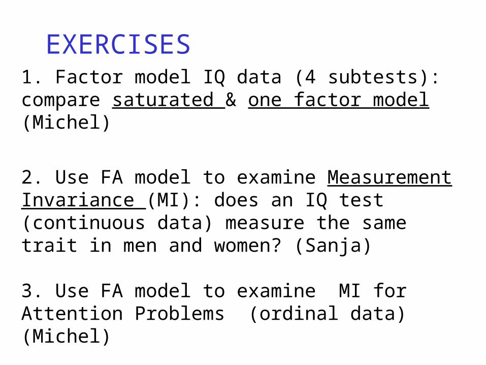
1. Factor model IQ data (4 subtests): compare saturated & one factor model (Michel)
2. Use FA model to examine Measurement Invariance (MI): does an IQ test (continuous data) measure the same trait in men and women? (Sanja)
3. Use FA model to examine MI for Attention Problems (ordinal data) (Michel)
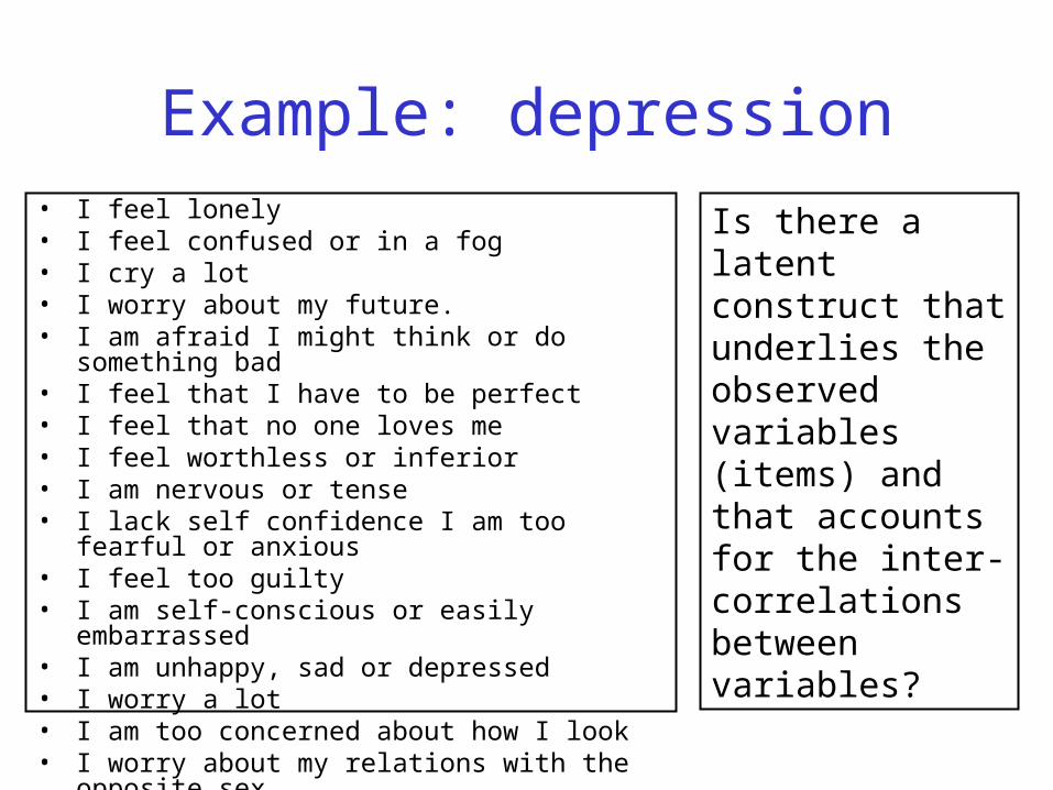
Example: depression• I feel lonely• I feel confused or in a fog• I cry a lot• I worry about my future.• I am afraid I might think or do something bad• I feel that I have to be perfect• I feel that no one loves me• I feel worthless or inferior• I am nervous or tense• I lack self confidence I am too fearful or anxious• I feel too guilty• I am self-conscious or easily embarrassed• I am unhappy, sad or depressed• I worry a lot• I am too concerned about how I look • I worry about my relations with the opposite sex
Is there a latent construct that underlies the observed variables (items) and that accounts for the inter-correlations between variables?
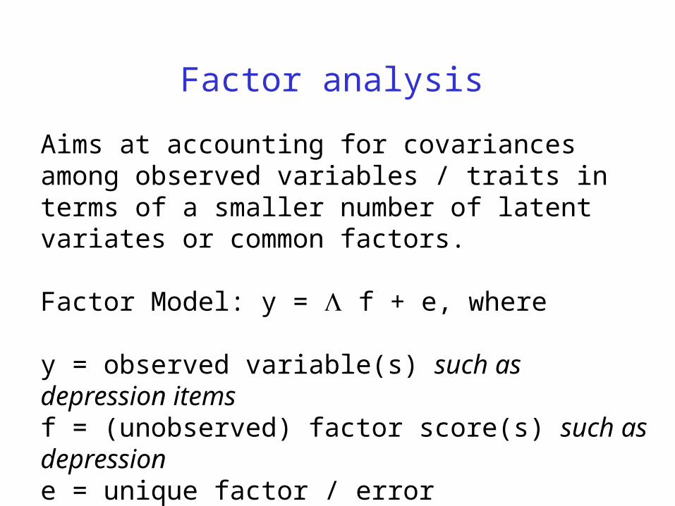
Aims at accounting for covariances among observed variables / traits in terms of a smaller number of latent variates or common factors.
Factor Model: y = f + e, where
y = observed variable(s) such as depression itemsf = (unobserved) factor score(s) such as depressione = unique factor / error = matrix of factor loadings
Factor analysis
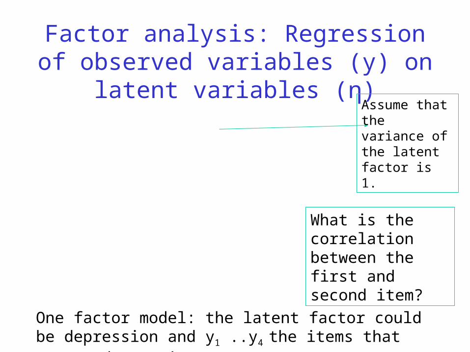
Factor analysis: Regression of observed variables (y) on latent variables (η)
One factor model: the latent factor could be depression and y1 ..y4 the items that assess depressive symptoms.
What is the correlation between the first and second item?
Assume that the variance of the latent factor is 1.
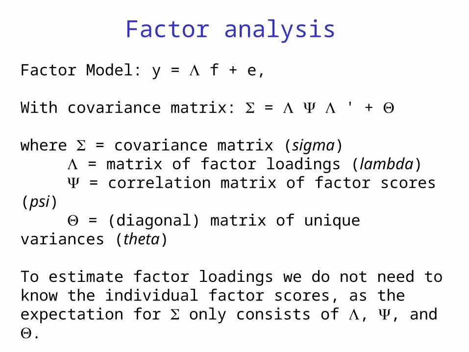
Factor Model: y = f + e,
With covariance matrix: = ' +
where = covariance matrix (sigma) = matrix of factor loadings (lambda) = correlation matrix of factor scores (psi) = (diagonal) matrix of unique variances (theta)
To estimate factor loadings we do not need to know the individual factor scores, as the expectation for only consists of , , and .
• C. Spearman (1904): General intelligence, objectively determined and measured. American Journal of Psychology, 201-293
• L.L. Thurstone (1947): Multiple Factor Analysis, University of Chicago Press
Factor analysis
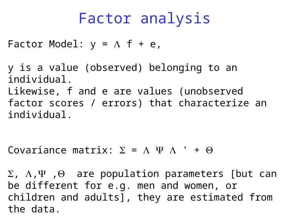
Factor Model: y = f + e,
y is a value (observed) belonging to an individual.Likewise, f and e are values (unobserved factor scores / errors) that characterize an individual.
Covariance matrix: = ' +
, , , are population parameters [but can be different for e.g. men and women, or children and adults], they are estimated from the data.
Factor analysis
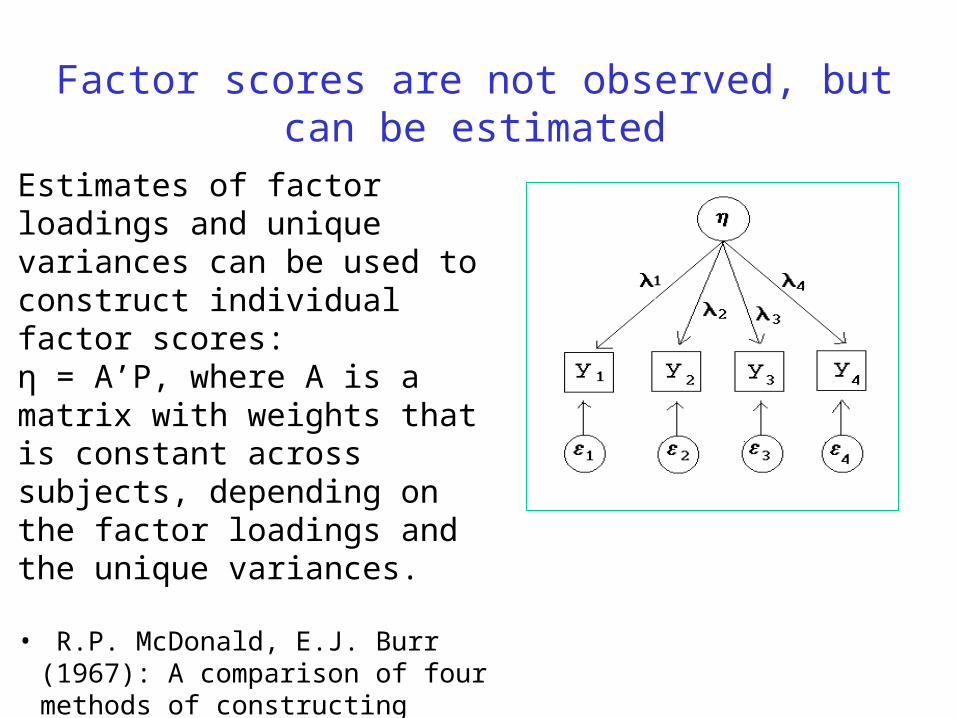
Estimates of factor loadings and unique variances can be used to construct individual factor scores: η = A’P, where A is a matrix with weights that is constant across subjects, depending on the factor loadings and the unique variances.
• R.P. McDonald, E.J. Burr (1967): A comparison of four methods of constructing factor scores. Psychometrika, 381-401
• W.E. Saris, M. dePijper, J. Mulder (1978): Optimal procedures for estimation of factor scores. Sociological Methods & Research, 85-106
Factor scores are not observed, but can be estimated


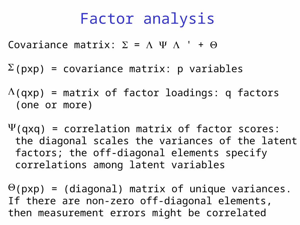
Covariance matrix: = ' +
(pxp) = covariance matrix: p variables
(qxp) = matrix of factor loadings: q factors (one or more)
(qxq) = correlation matrix of factor scores: the diagonal scales the variances of the latent factors; the off-diagonal elements specify correlations among latent variables
(pxp) = (diagonal) matrix of unique variances.If there are non-zero off-diagonal elements, then measurement errors might be correlated
Factor analysis
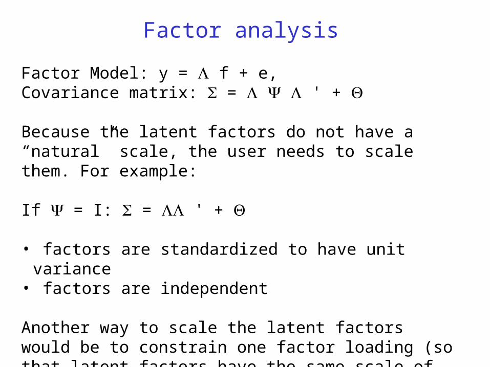
Factor Model: y = f + e,Covariance matrix: = ' +
Because the latent factors do not have a “natural” scale, the user needs to scale them. For example:
If = I: = ' +
• factors are standardized to have unit variance• factors are independent
Another way to scale the latent factors would be to constrain one factor loading (so that latent factors have the same scale of measurement as the observed variable).
Factor analysis
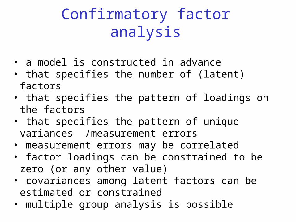
• a model is constructed in advance• that specifies the number of (latent) factors• that specifies the pattern of loadings on the factors• that specifies the pattern of unique variances /measurement
errors• measurement errors may be correlated• factor loadings can be constrained to be zero (or any other value)• covariances among latent factors can be estimated or constrained• multiple group analysis is possible
We can TEST if these constraints are consistent with the data.
Confirmatory factor analysis
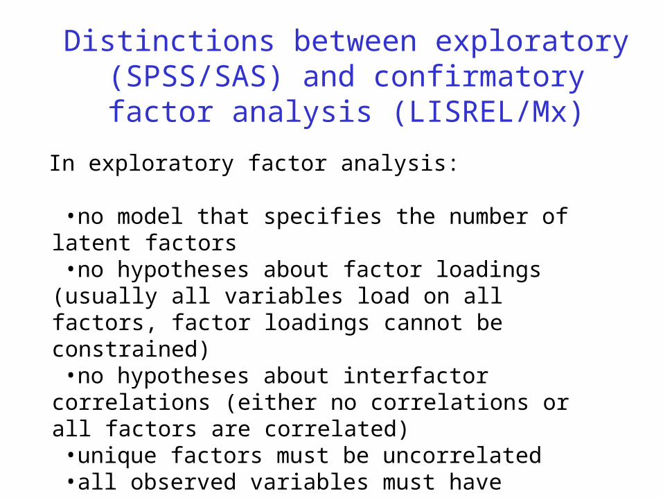
In exploratory factor analysis:
•no model that specifies the number of latent factors•no hypotheses about factor loadings (usually all variables
load on all factors, factor loadings cannot be constrained)•no hypotheses about interfactor correlations (either no
correlations or all factors are correlated)•unique factors must be uncorrelated•all observed variables must have specific variances•no multiple group analysis possible•under-identification of parameters
Distinctions between exploratory (SPSS/SAS) and confirmatory factor analysis (LISREL/Mx)


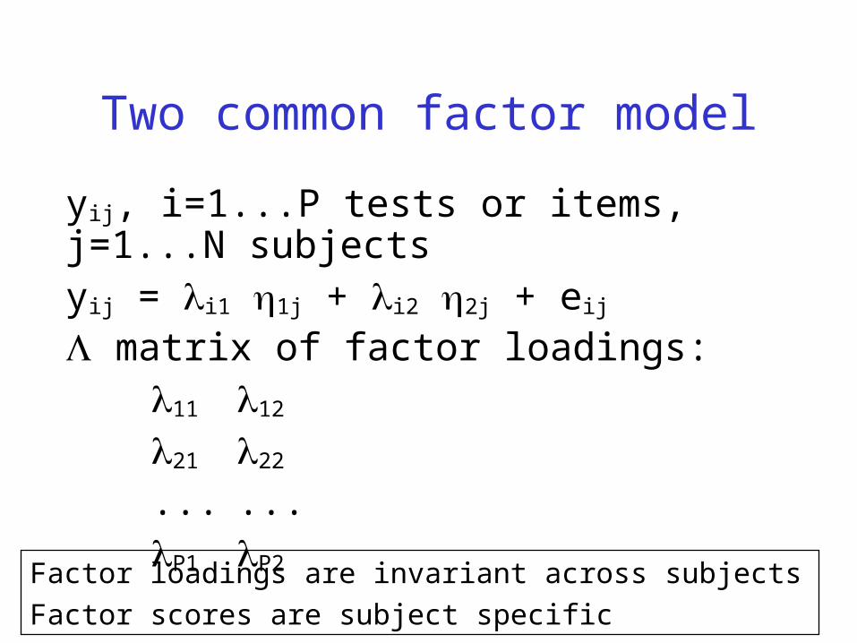
Two common factor model
yij, i=1...P tests or items, j=1...N subjectsyij = i1 1j + i2 2j + eij
matrix of factor loadings:11 12
21 22
... ...P1 P2
Factor loadings are invariant across subjects
Factor scores are subject specific
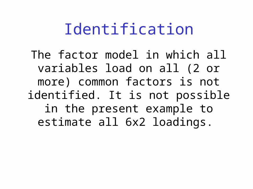
Identification
The factor model in which all variables load on all (2 or more) common factors is not identified. It is not possible in the present
example to estimate all 6x2 loadings.
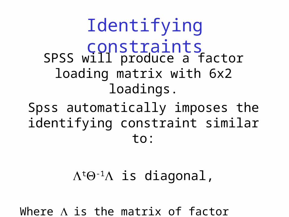
Identifying constraintsSPSS will produce a factor loading matrix with
6x2 loadings.
Spss automatically imposes the identifying constraint similar to:
t-1 is diagonal,
Where is the matrix of factor loadings and is the diagonal covariance matrix of the residuals (eij).
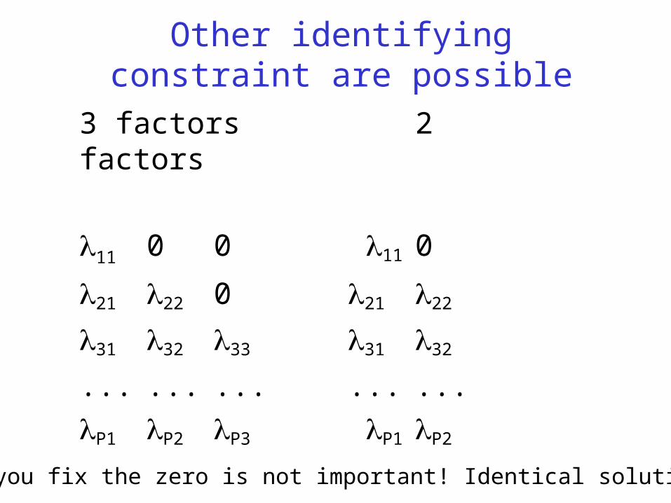
Other identifying constraint are possible
3 factors 2 factors
11 0 0 11 0
21 22 0 21 22
31 32 33 31 32
... ... ... ... ...
P1 P2 P3 P1 P2
Where you fix the zero is not important! Identical solutions.
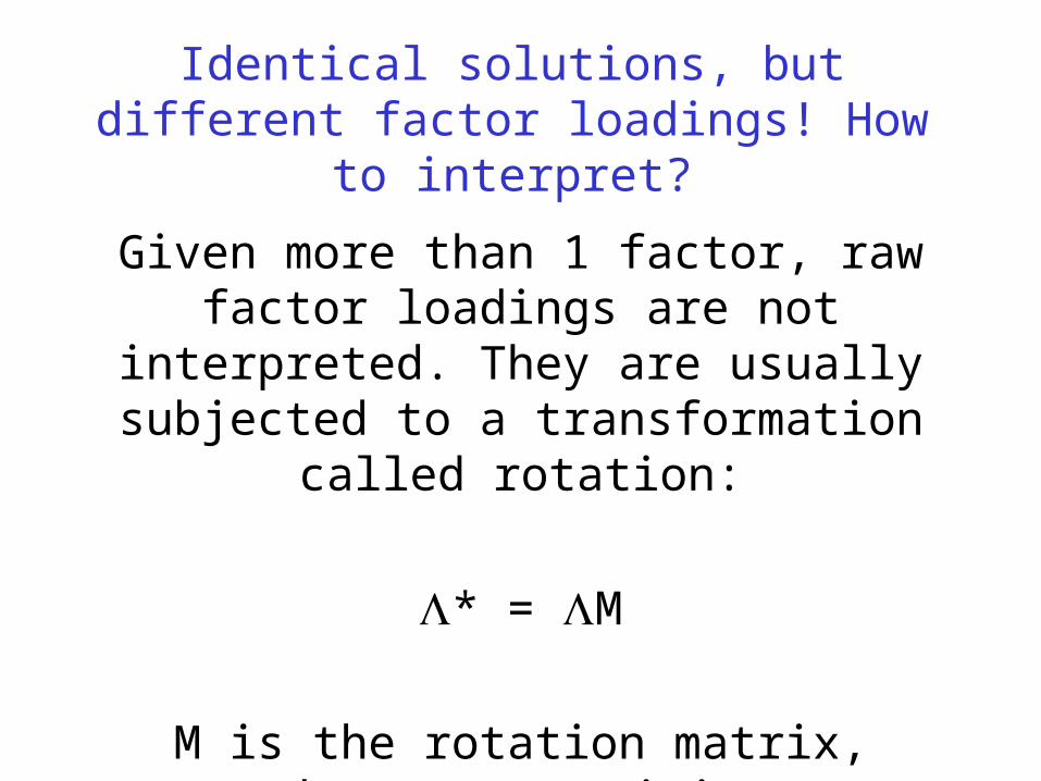
Identical solutions, but different factor loadings! How to interpret?
Given more than 1 factor, raw factor loadings are not interpreted. They are usually subjected
to a transformation called rotation:
* = M
M is the rotation matrix, chosen to maximize “interpretability” of loadings
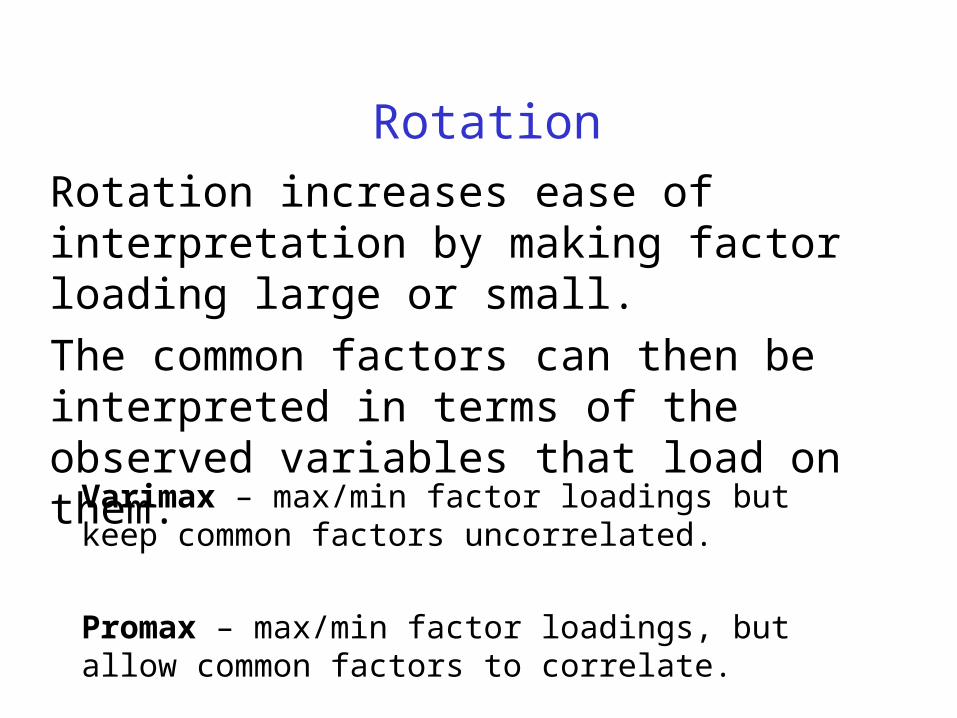
Rotation
Rotation increases ease of interpretation by making factor loading large or small.
The common factors can then be interpreted in terms of the observed variables that load on them.
Varimax – max/min factor loadings but keep common factors uncorrelated.
Promax – max/min factor loadings, but allow common factors to correlate.
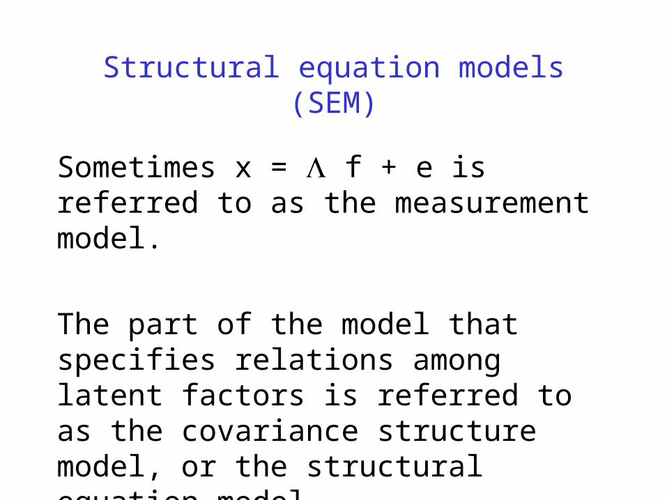
Structural equation models (SEM)
Sometimes x = f + e is referred to as the measurement model.
The part of the model that specifies relations among latent factors is referred to as the covariance structure model, or the structural equation model.

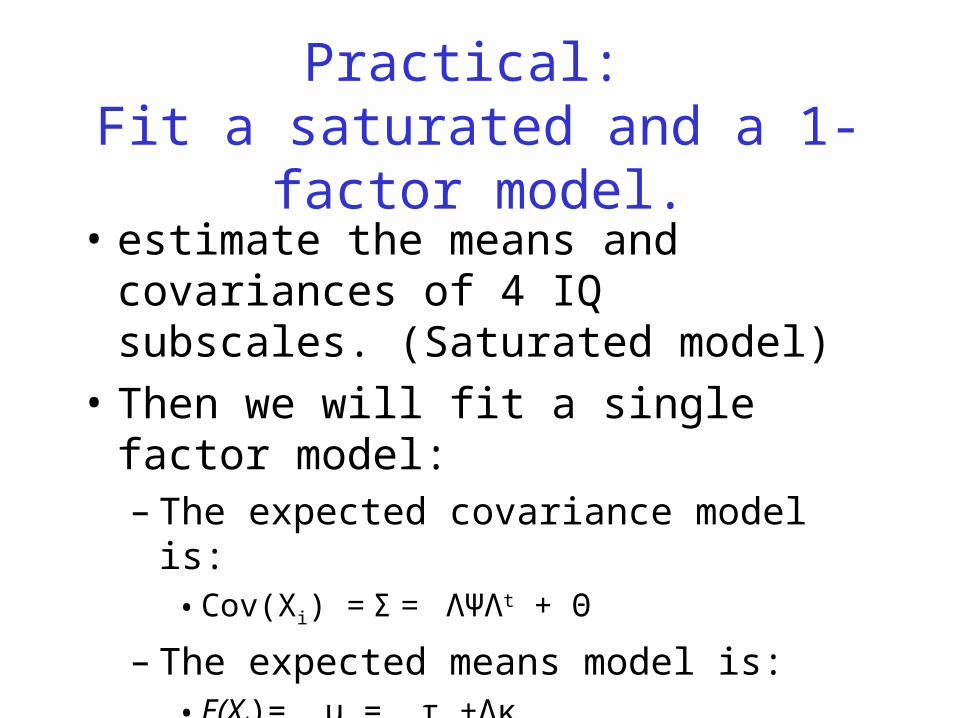
Practical: Fit a saturated and a 1-factor model.
• estimate the means and covariances of 4 IQ subscales. (Saturated model)
• Then we will fit a single factor model:– The expected covariance model is:
• Cov(Xi) = Σ = ΛΨΛt + Θ
– The expected means model is:• E(Xi)= μ = τ +Λκ
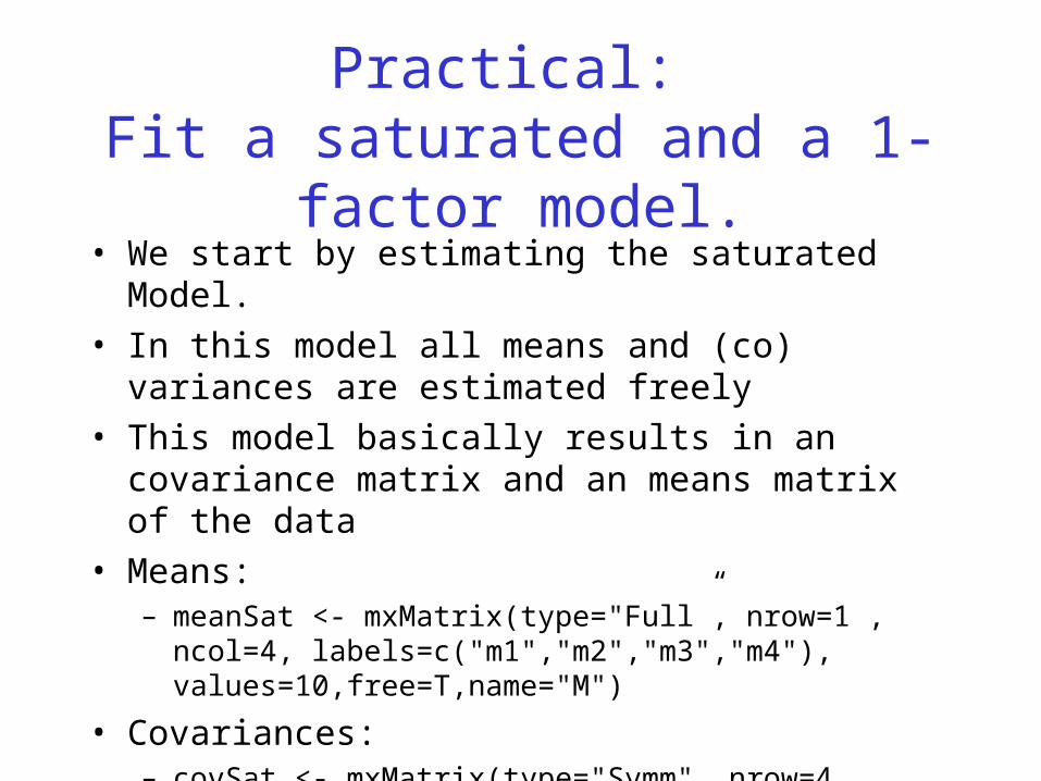
• We start by estimating the saturated Model.
• In this model all means and (co) variances are estimated freely
• This model basically results in an covariance matrix and an means matrix of the data
• Means:– meanSat <- mxMatrix(type="Full”, nrow=1 , ncol=4,
labels=c("m1","m2","m3","m4"), values=10,free=T,name="M")
• Covariances:– covSat <- mxMatrix(type="Symm", nrow=4, ncol=4, free=T,
values=startcov, name="cov")
Practical: Fit a saturated and a 1-factor model.
Practical:Fit a saturated and a 1-factor model.
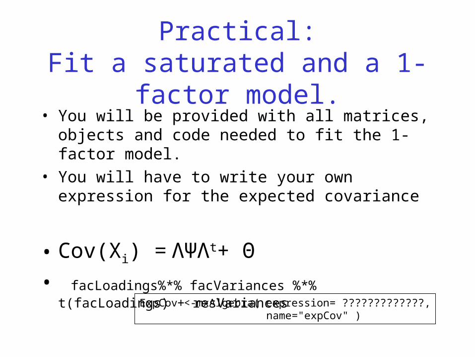
• You will be provided with all matrices, objects and code needed to fit the 1-factor model.
• You will have to write your own expression for the expected covariance
• Cov(Xi) = ΛΨΛt+ Θ
• facLoadings%*% facVariances %*% t(facLoadings) + resVariances
ExpCov <-mxAlgebra( expression= ?????????????, name="expCov" )
Measurement invariancein the linear factor model: practical
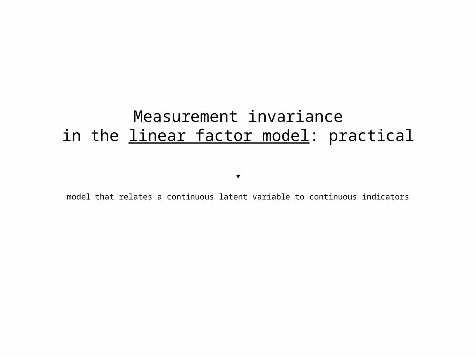
Measurement invariancein the linear factor model: practical
model that relates a continuous latent variable to continuous indicators
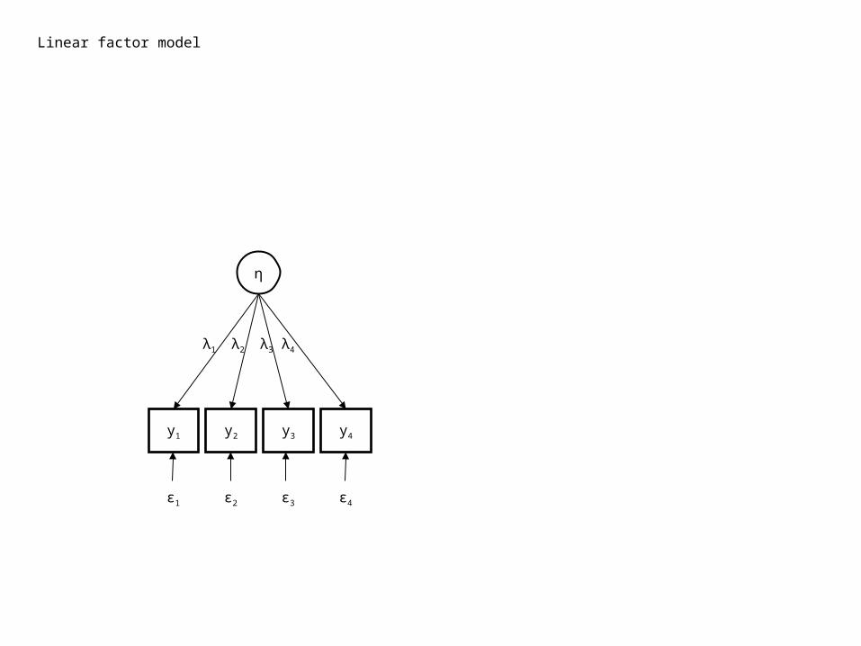
Linear factor model
y2
η
y3 y4y1
λ1 λ2 λ3 λ4
ε1 ε2 ε3 ε4
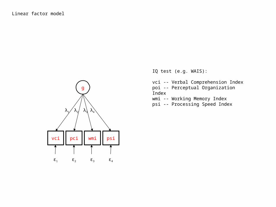
Linear factor model
pci
g
wmi psivci
λ1 λ2 λ3 λ4
ε1 ε2 ε3 ε4
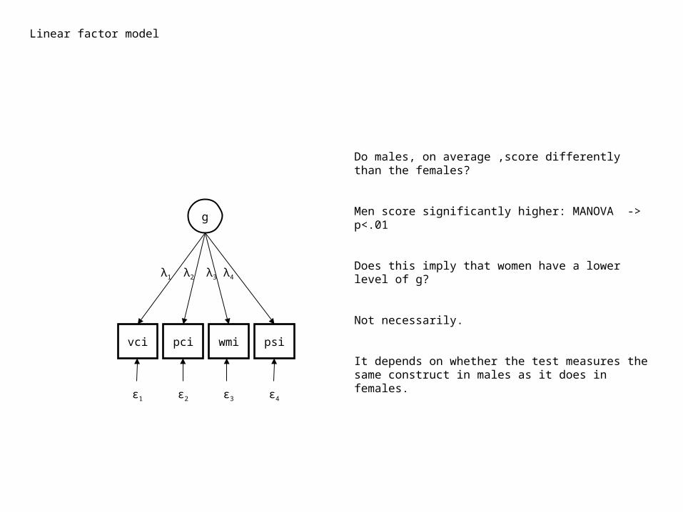
IQ test (e.g. WAIS):
vci -- Verbal Comprehension Index poi -- Perceptual Organization Indexwmi -- Working Memory Index psi -- Processing Speed Index
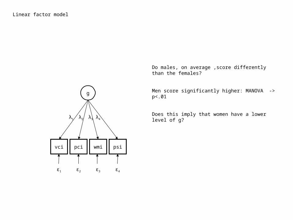
Linear factor model
Do males, on average ,score differently than the females?
Men score significantly higher: MANOVA -> p<.01
Does this imply that women have a lower level of g?
pci
g
wmi psivci
λ1 λ2 λ3 λ4
ε1 ε2 ε3 ε4
Linear factor model
Do males, on average ,score differently than the females?
Men score significantly higher: MANOVA -> p<.01
Does this imply that women have a lower level of g?
Not necessarily.
It depends on whether the test measures the same construct in males as it does in females.pci
g
wmi psivci
λ1 λ2 λ3 λ4
ε1 ε2 ε3 ε4
Linear factor model
pci
g
wmi psivci
λ1 λ2 λ3 λ4
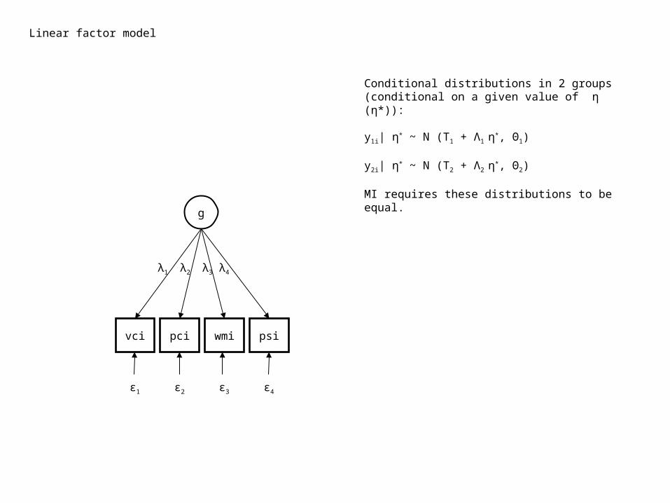
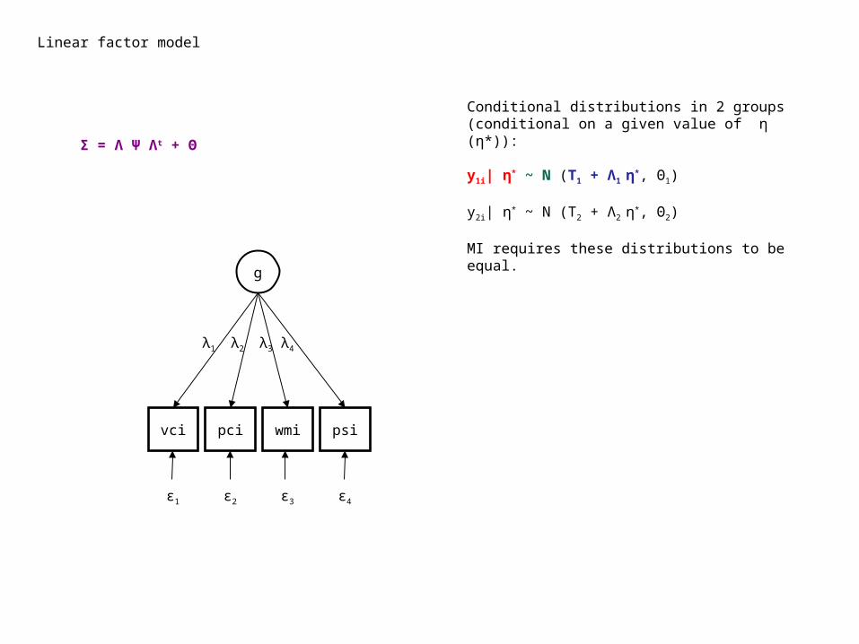
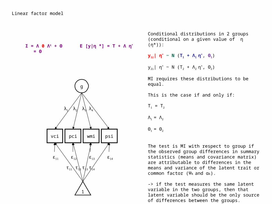
Conditional distributions in 2 groups (conditional on a given value of η (η*)):
y1i| η* ~ N (Τ1 + Λ1 η*, Θ1)
y2i| η* ~ N (Τ2 + Λ2 η*, Θ2)
MI requires these distributions to be equal.
ε1 ε2 ε3 ε4
Linear factor model
pci
g
wmi psivci
λ1 λ2 λ3 λ4
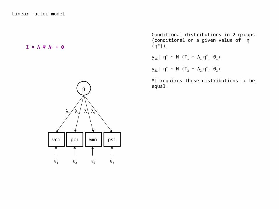
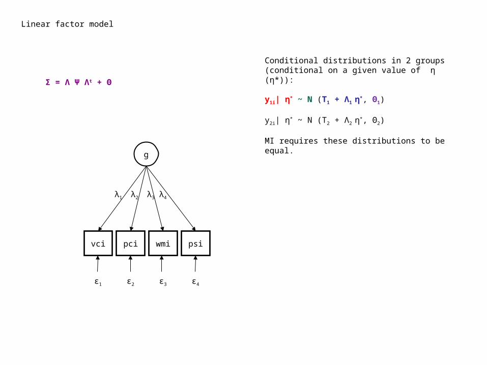
Conditional distributions in 2 groups (conditional on a given value of η (η*)):
y1i| η* ~ N (Τ1 + Λ1 η*, Θ1)
y2i| η* ~ N (Τ2 + Λ2 η*, Θ2)
MI requires these distributions to be equal.
ε1 ε2 ε3 ε4
Σ = Λ Ψ Λt + Θ

Linear factor model
pci
g
wmi psivci
λ1 λ2 λ3 λ4
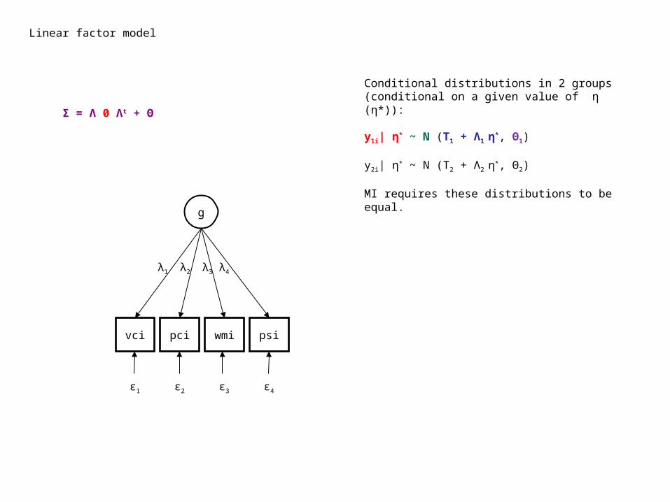
Conditional distributions in 2 groups (conditional on a given value of η (η*)):
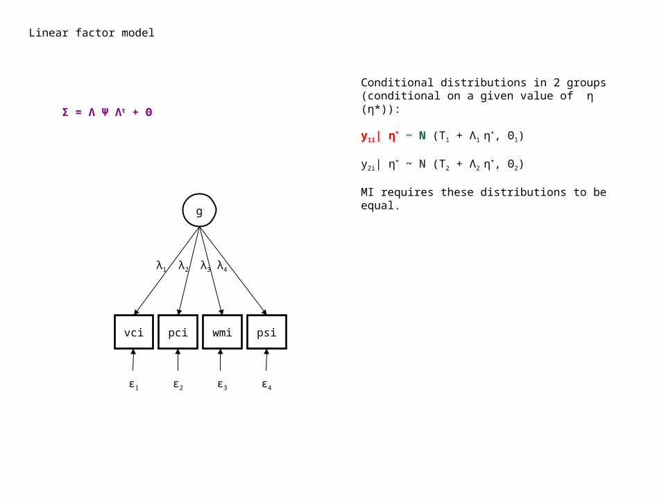
y1i| η* ~ N (Τ1 + Λ1 η*, Θ1)
y2i| η* ~ N (Τ2 + Λ2 η*, Θ2)
MI requires these distributions to be equal.
ε1 ε2 ε3 ε4
Σ = Λ Ψ Λt + Θ
Linear factor model
pci
g
wmi psivci
λ1 λ2 λ3 λ4
Conditional distributions in 2 groups (conditional on a given value of η (η*)):
y1i| η* ~ N (Τ1 + Λ1 η*, Θ1)
y2i| η* ~ N (Τ2 + Λ2 η*, Θ2)
MI requires these distributions to be equal.
ε1 ε2 ε3 ε4
Σ = Λ Ψ Λt + Θ
Linear factor model
pci
g
wmi psivci
λ1 λ2 λ3 λ4
Conditional distributions in 2 groups (conditional on a given value of η (η*)):
y1i| η* ~ N (Τ1 + Λ1 η*, Θ1)
y2i| η* ~ N (Τ2 + Λ2 η*, Θ2)
MI requires these distributions to be equal.
ε1 ε2 ε3 ε4
Σ = Λ Ψ Λt + Θ
Linear factor model
pci
g
wmi psivci
λ1 λ2 λ3 λ4
Conditional distributions in 2 groups (conditional on a given value of η (η*)):
y1i| η* ~ N (Τ1 + Λ1 η*, Θ1)
y2i| η* ~ N (Τ2 + Λ2 η*, Θ2)
MI requires these distributions to be equal.
ε1 ε2 ε3 ε4
Σ = Λ Ψ Λt + Θ
Linear factor model
pci
g
wmi psivci
λ1 λ2 λ3 λ4
Conditional distributions in 2 groups (conditional on a given value of η (η*)):
y1i| η* ~ N (Τ1 + Λ1 η*, Θ1)
y2i| η* ~ N (Τ2 + Λ2 η*, Θ2)
MI requires these distributions to be equal.
ε1 ε2 ε3 ε4
Σ = Λ 0 Λt + Θ

Linear factor model
pci
g
wmi psivci
λ1 λ2 λ3 λ4
Conditional distributions in 2 groups (conditional on a given value of η (η*)):
y1i| η* ~ N (Τ1 + Λ1 η*, Θ1)
y2i| η* ~ N (Τ2 + Λ2 η*, Θ2)
MI requires these distributions to be equal.
ε1 ε2 ε3 ε4
Σ = Λ 0 Λt + Θ = Θ
Linear factor model
pci
g
wmi psivci
λ1 λ2 λ3 λ4
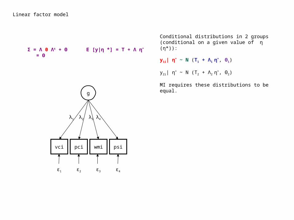
Conditional distributions in 2 groups (conditional on a given value of η (η*)):
y1i| η* ~ N (Τ1 + Λ1 η*, Θ1)
y2i| η* ~ N (Τ2 + Λ2 η*, Θ2)
MI requires these distributions to be equal.
ε1 ε2 ε3 ε4
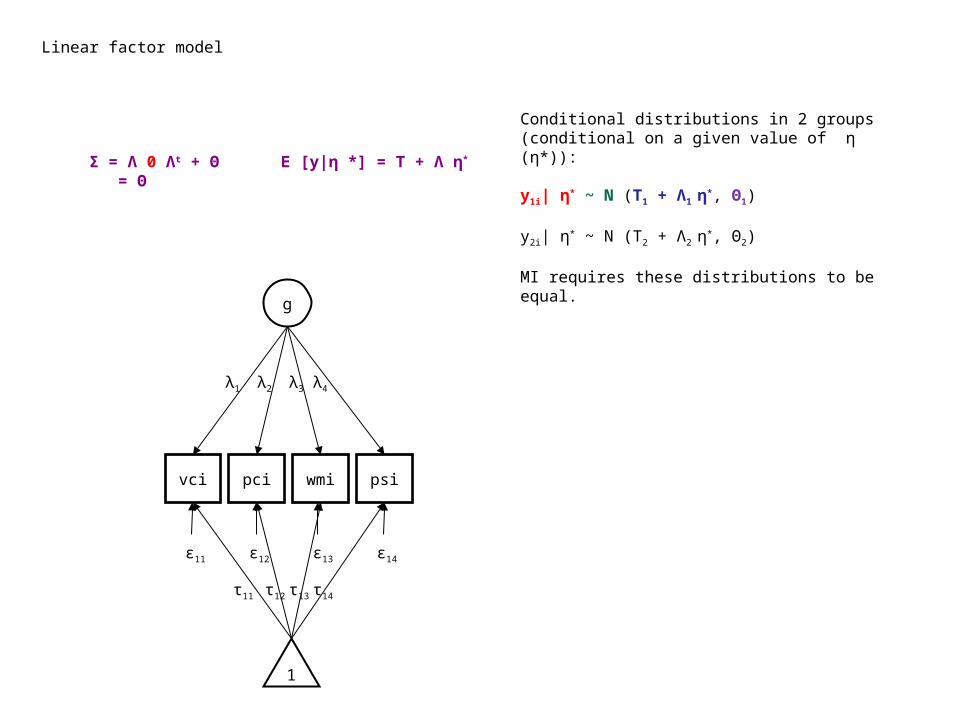
Σ = Λ 0 Λt + Θ = Θ
E [y|η *] = Τ + Λ η*
Linear factor model
pci
g
wmi psivci
λ1 λ2 λ3 λ4
Conditional distributions in 2 groups (conditional on a given value of η (η*)):
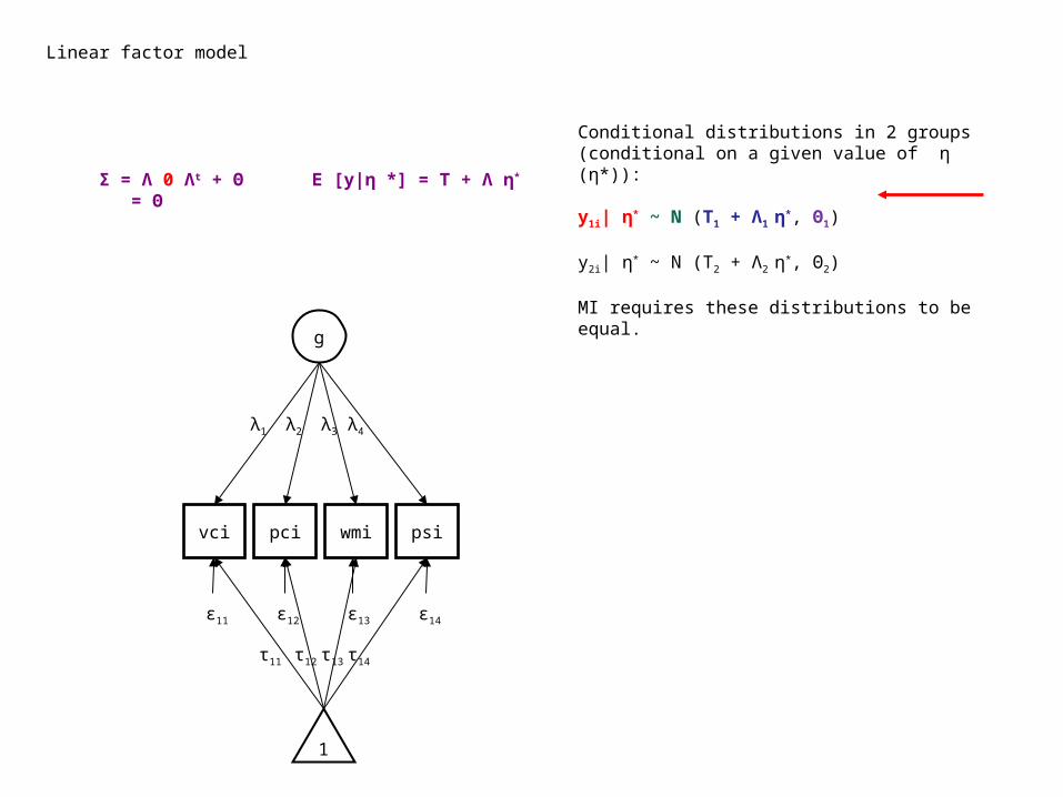
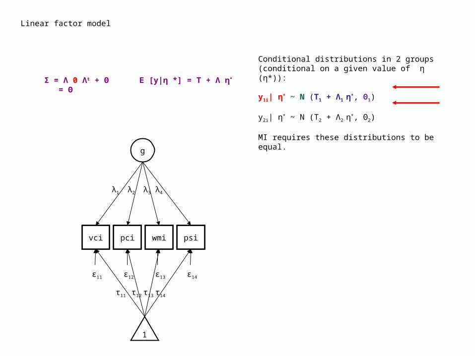
y1i| η* ~ N (Τ1 + Λ1 η*, Θ1)
y2i| η* ~ N (Τ2 + Λ2 η*, Θ2)
MI requires these distributions to be equal.
Σ = Λ 0 Λt + Θ = Θ
E [y|η *] = Τ + Λ η*
ε11 ε12 ε13 ε14
1
τ1
1
τ1
2
τ1
3
τ1
4
Linear factor model
pci
g
wmi psivci
λ1 λ2 λ3 λ4
Conditional distributions in 2 groups (conditional on a given value of η (η*)):
y1i| η* ~ N (Τ1 + Λ1 η*, Θ1)
y2i| η* ~ N (Τ2 + Λ2 η*, Θ2)
MI requires these distributions to be equal.
Σ = Λ 0 Λt + Θ = Θ
E [y|η *] = Τ + Λ η*
ε11 ε12 ε13 ε14
1
τ1
1
τ1
2
τ1
3
τ1
4
Linear factor model
pci
g
wmi psivci
λ1 λ2 λ3 λ4
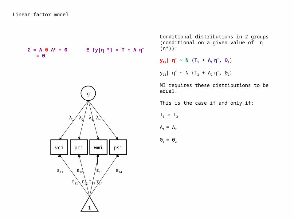
Conditional distributions in 2 groups (conditional on a given value of η (η*)):
y1i| η* ~ N (Τ1 + Λ1 η*, Θ1)
y2i| η* ~ N (Τ2 + Λ2 η*, Θ2)
MI requires these distributions to be equal.
This is the case if and only if:
Τ1 = Τ2
Λ1 = Λ2
Θ1 = Θ2
Σ = Λ 0 Λt + Θ = Θ
E [y|η *] = Τ + Λ η*
ε11 ε12 ε13 ε14
1
τ1
1
τ1
2
τ1
3
τ1
4
Linear factor model
pci
g
wmi psivci
λ1 λ2 λ3 λ4
Conditional distributions in 2 groups (conditional on a given value of η (η*)):
y1i| η* ~ N (Τ1 + Λ1 η*, Θ1)
y2i| η* ~ N (Τ2 + Λ2 η*, Θ2)
MI requires these distributions to be equal.
This is the case if and only if:
Τ1 = Τ2
Λ1 = Λ2
Θ1 = Θ2
The test is MI with respect to group if the observed group differences in summary statistics (means and covariance matrix) are attributable to differences in the means and variance of the latent trait or common factor (Ψk and αk).
-> if the test measures the same latent variable in the two groups, then that latent variable should be the only source of differences between the groups.
Σ = Λ 0 Λt + Θ = Θ
E [y|η *] = Τ + Λ η*
ε11 ε12 ε13 ε14
1
τ1
1
τ1
2
τ1
3
τ1
4
Linear factor model
y2
g
y3 y4y1
λ1 λ2 λ3 λ4
ε1 ε2 ε3 ε4
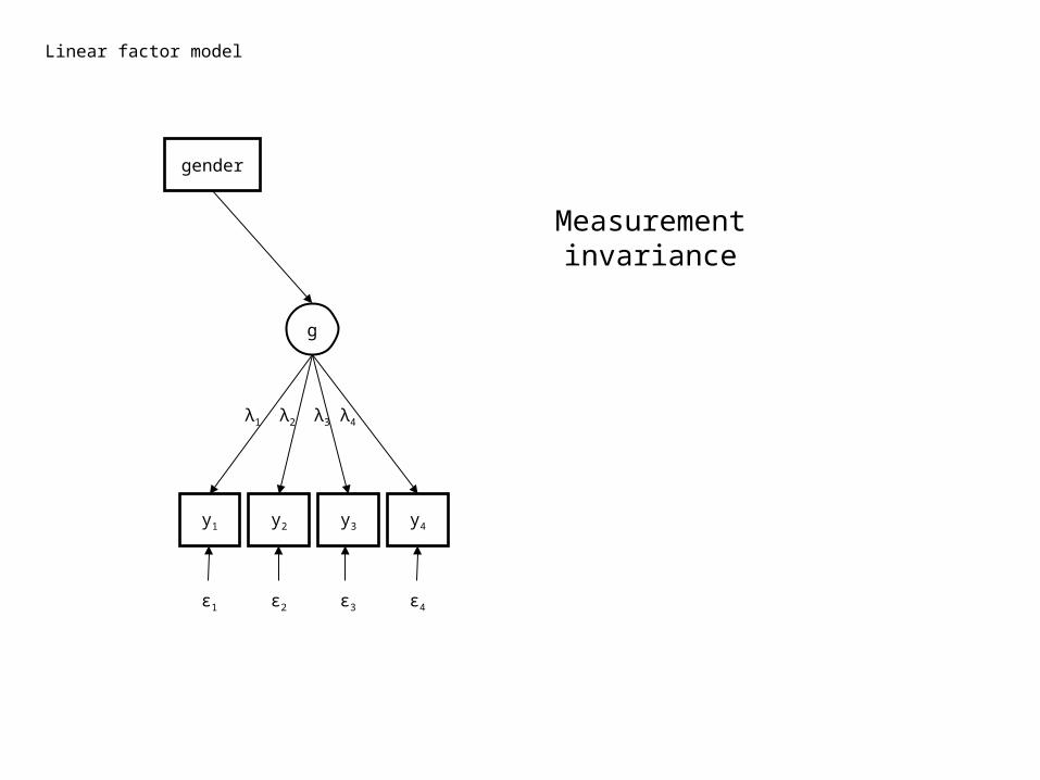
gender
Measurement invariance
Linear factor model
y2
g
y3 y4y1
λ1 λ2 λ3 λ4
ε1 ε2 ε3 ε4
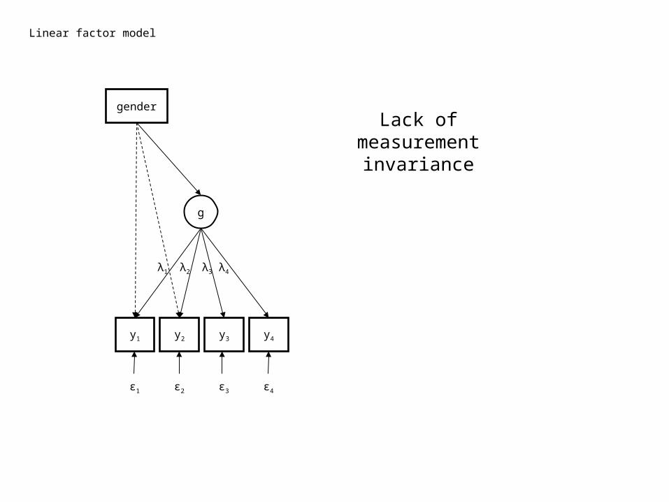
genderLack of
measurement invariance
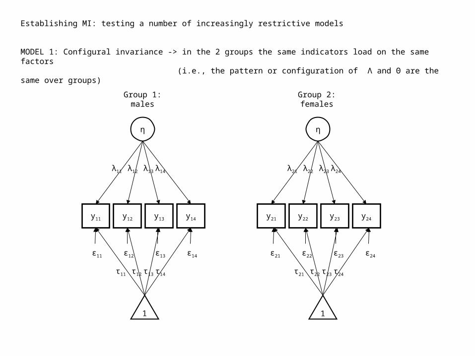
Establishing MI: testing a number of increasingly restrictive models
MODEL 1: Configural invariance -> in the 2 groups the same indicators load on the same factors (i.e., the pattern or configuration of Λ and Θ are the same over groups)
y12
η
y13 y14y11
λ1
1
λ1
2
λ1
3
λ1
4
ε11 ε12 ε13 ε14
y22
η
y23 y24y21
λ2
1
λ2
2
λ2
3
λ2
4
1
τ1
1
τ1
2
τ1
3
τ1
4
ε21 ε22 ε23 ε24
1
τ2
1
τ2
2
τ2
3
τ2
4
Group 2: females
Group 1: males
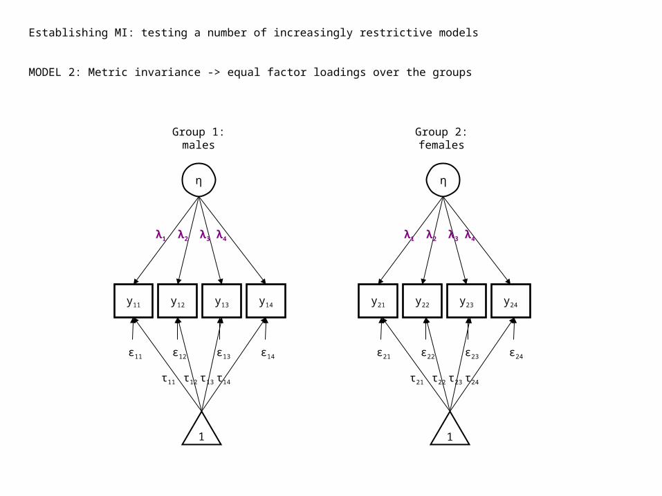
Establishing MI: testing a number of increasingly restrictive models
MODEL 2: Metric invariance -> equal factor loadings over the groups
y12
η
y13 y14y11
λ1 λ2 λ3 λ4
ε11 ε12 ε13 ε14
y22
η
y23 y24y21
1
τ1
1
τ1
2
τ1
3
τ1
4
ε21 ε22 ε23 ε24
1
τ2
1
τ2
2
τ2
3
τ2
4
Group 2: females
Group 1: males
λ1 λ2 λ3 λ4
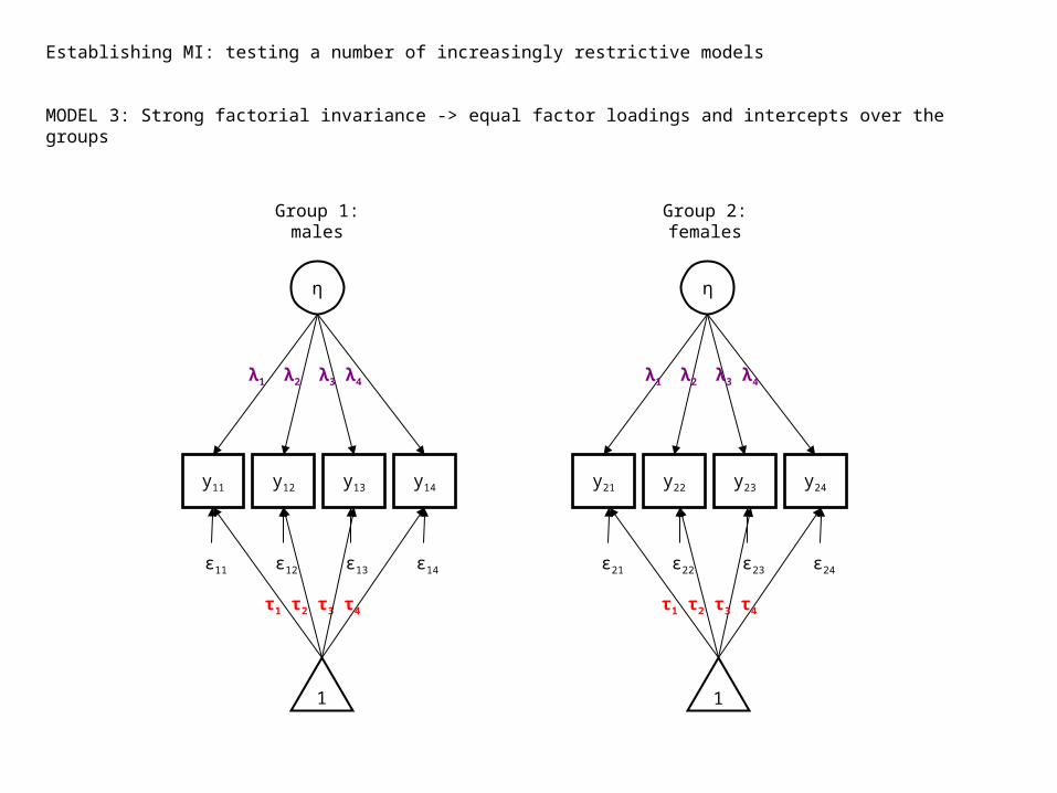
Establishing MI: testing a number of increasingly restrictive models
MODEL 3: Strong factorial invariance -> equal factor loadings and intercepts over the groups
y12
η
y13 y14y11
λ1 λ2 λ3 λ4
ε11 ε12 ε13 ε14
y22
η
y23 y24y21
1
τ1 τ2 τ3 τ4
ε21 ε22 ε23 ε24
1
Group 2: females
Group 1: males
λ1 λ2 λ3 λ4
τ1 τ2 τ3 τ4
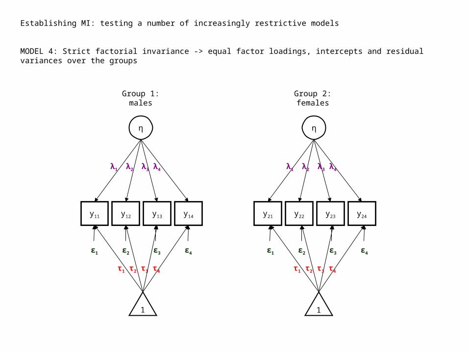
Establishing MI: testing a number of increasingly restrictive models
MODEL 4: Strict factorial invariance -> equal factor loadings, intercepts and residual variances over the groups
y12
η
y13 y14y11
λ1 λ2 λ3 λ4
ε1 ε2 ε3 ε4
y22
η
y23 y24y21
1
τ1 τ2 τ3 τ4
ε1 ε2 ε3 ε4
1
Group 2: females
Group 1: males
λ1 λ2 λ3 λ4
τ1 τ2 τ3 τ4
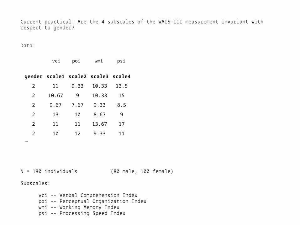
Current practical: Are the 4 subscales of the WAIS-III measurement invariant with respect to gender?
Data:
N = 180 individuals (80 male, 100 female)
Subscales: vci -- Verbal Comprehension Index poi -- Perceptual Organization Index wmi -- Working Memory Index psi -- Processing Speed Index
gender scale1 scale2 scale3 scale4
2 11 9.33 10.33 13.5
2 10.67 9 10.33 15
2 9.67 7.67 9.33 8.5
2 13 10 8.67 9
2 11 11 13.67 17
2 10 12 9.33 11…
vci poi wmi psi
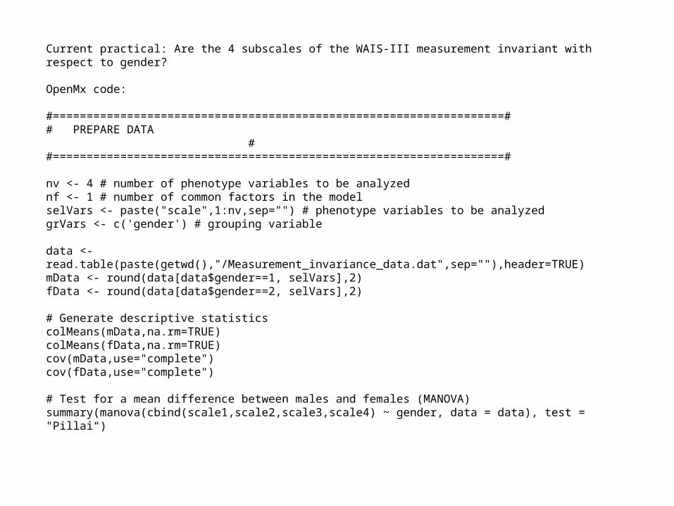
Current practical: Are the 4 subscales of the WAIS-III measurement invariant with respect to gender?
OpenMx code:
#===================================================================## PREPARE DATA ##===================================================================#
nv <- 4 # number of phenotype variables to be analyzednf <- 1 # number of common factors in the modelselVars <- paste("scale",1:nv,sep="") # phenotype variables to be analyzedgrVars <- c('gender') # grouping variable
data <- read.table(paste(getwd(),"/Measurement_invariance_data.dat",sep=""),header=TRUE)mData <- round(data[data$gender==1, selVars],2)fData <- round(data[data$gender==2, selVars],2)
# Generate descriptive statisticscolMeans(mData,na.rm=TRUE)colMeans(fData,na.rm=TRUE)cov(mData,use="complete")cov(fData,use="complete")
# Test for a mean difference between males and females (MANOVA)summary(manova(cbind(scale1,scale2,scale3,scale4) ~ gender, data = data), test = "Pillai“)
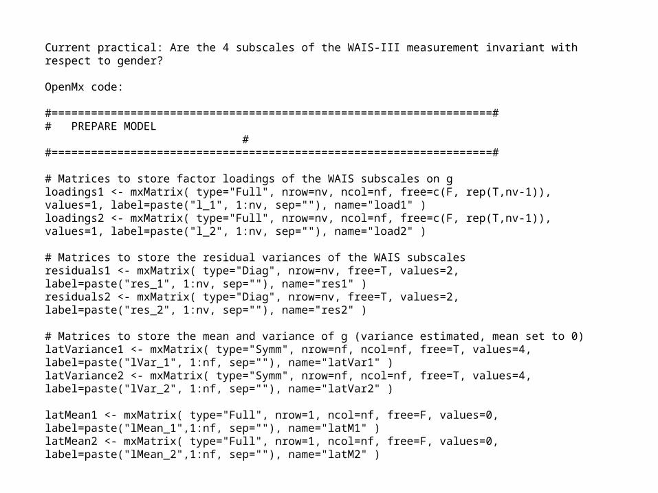
Current practical: Are the 4 subscales of the WAIS-III measurement invariant with respect to gender?
OpenMx code:
#===================================================================## PREPARE MODEL ##===================================================================#
# Matrices to store factor loadings of the WAIS subscales on gloadings1 <- mxMatrix( type="Full", nrow=nv, ncol=nf, free=c(F, rep(T,nv-1)), values=1, label=paste("l_1", 1:nv, sep=""), name="load1" )loadings2 <- mxMatrix( type="Full", nrow=nv, ncol=nf, free=c(F, rep(T,nv-1)), values=1, label=paste("l_2", 1:nv, sep=""), name="load2" )
# Matrices to store the residual variances of the WAIS subscalesresiduals1 <- mxMatrix( type="Diag", nrow=nv, free=T, values=2, label=paste("res_1", 1:nv, sep=""), name="res1" )residuals2 <- mxMatrix( type="Diag", nrow=nv, free=T, values=2, label=paste("res_2", 1:nv, sep=""), name="res2" )
# Matrices to store the mean and variance of g (variance estimated, mean set to 0)latVariance1 <- mxMatrix( type="Symm", nrow=nf, ncol=nf, free=T, values=4, label=paste("lVar_1", 1:nf, sep=""), name="latVar1" ) latVariance2 <- mxMatrix( type="Symm", nrow=nf, ncol=nf, free=T, values=4, label=paste("lVar_2", 1:nf, sep=""), name="latVar2" )
latMean1 <- mxMatrix( type="Full", nrow=1, ncol=nf, free=F, values=0,label=paste("lMean_1",1:nf, sep=""), name="latM1" ) latMean2 <- mxMatrix( type="Full", nrow=1, ncol=nf, free=F, values=0,label=paste("lMean_2",1:nf, sep=""), name="latM2" )
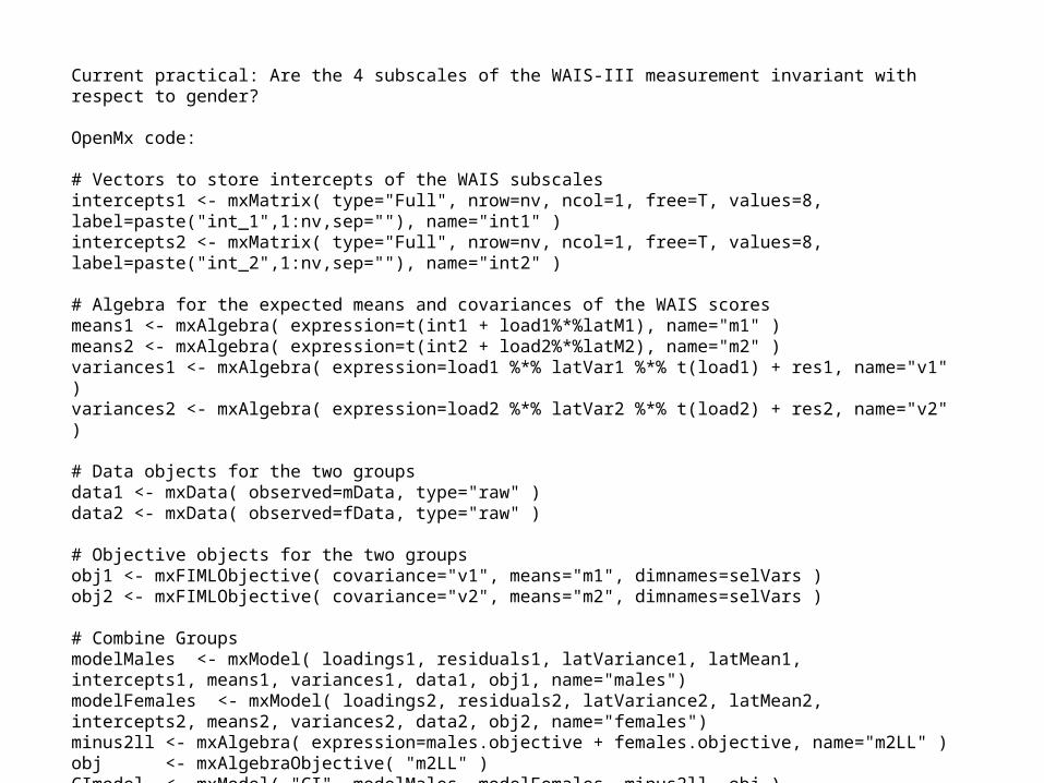
Current practical: Are the 4 subscales of the WAIS-III measurement invariant with respect to gender?
OpenMx code:
# Vectors to store intercepts of the WAIS subscalesintercepts1 <- mxMatrix( type="Full", nrow=nv, ncol=1, free=T, values=8,label=paste("int_1",1:nv,sep=""), name="int1" )intercepts2 <- mxMatrix( type="Full", nrow=nv, ncol=1, free=T, values=8,label=paste("int_2",1:nv,sep=""), name="int2" )
# Algebra for the expected means and covariances of the WAIS scoresmeans1 <- mxAlgebra( expression=t(int1 + load1%*%latM1), name="m1" )means2 <- mxAlgebra( expression=t(int2 + load2%*%latM2), name="m2" )variances1 <- mxAlgebra( expression=load1 %*% latVar1 %*% t(load1) + res1, name="v1" )variances2 <- mxAlgebra( expression=load2 %*% latVar2 %*% t(load2) + res2, name="v2" )
# Data objects for the two groupsdata1 <- mxData( observed=mData, type="raw" )data2 <- mxData( observed=fData, type="raw" )
# Objective objects for the two groupsobj1 <- mxFIMLObjective( covariance="v1", means="m1", dimnames=selVars )obj2 <- mxFIMLObjective( covariance="v2", means="m2", dimnames=selVars )
# Combine GroupsmodelMales <- mxModel( loadings1, residuals1, latVariance1, latMean1, intercepts1, means1, variances1, data1, obj1, name="males")modelFemales <- mxModel( loadings2, residuals2, latVariance2, latMean2,intercepts2, means2, variances2, data2, obj2, name="females")minus2ll <- mxAlgebra( expression=males.objective + females.objective, name="m2LL" )obj <- mxAlgebraObjective( "m2LL" )CImodel <- mxModel( "CI", modelMales, modelFemales, minus2ll, obj )
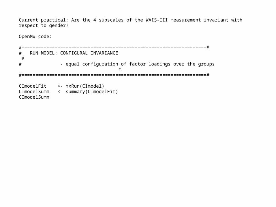
Current practical: Are the 4 subscales of the WAIS-III measurement invariant with respect to gender?
OpenMx code:
#===================================================================## RUN MODEL: CONFIGURAL INVARIANCE ## - equal configuration of factor loadings over the groups
##===================================================================#
CImodelFit <- mxRun(CImodel)CImodelSumm <- summary(CImodelFit)CImodelSumm
Current practical: Are the 4 subscales of the WAIS-III measurement invariant with respect to gender?
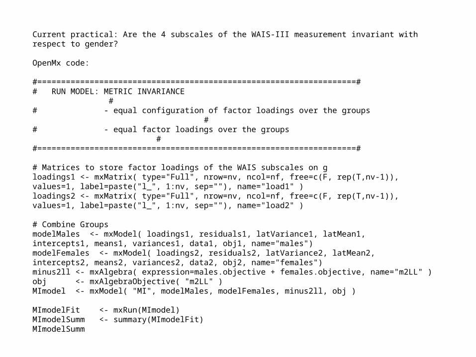
OpenMx code:
#===================================================================## RUN MODEL: METRIC INVARIANCE
## - equal configuration of factor loadings over the groups
## - equal factor loadings over the groups
##===================================================================#
# Matrices to store factor loadings of the WAIS subscales on gloadings1 <- mxMatrix( type="Full", nrow=nv, ncol=nf, free=c(F, rep(T,nv-1)), values=1, label=paste("l_", 1:nv, sep=""), name="load1" )loadings2 <- mxMatrix( type="Full", nrow=nv, ncol=nf, free=c(F, rep(T,nv-1)), values=1, label=paste("l_", 1:nv, sep=""), name="load2" )
# Combine GroupsmodelMales <- mxModel( loadings1, residuals1, latVariance1, latMean1, intercepts1, means1, variances1, data1, obj1, name="males")modelFemales <- mxModel( loadings2, residuals2, latVariance2, latMean2,intercepts2, means2, variances2, data2, obj2, name="females")minus2ll <- mxAlgebra( expression=males.objective + females.objective, name="m2LL" )obj <- mxAlgebraObjective( "m2LL" )MImodel <- mxModel( "MI", modelMales, modelFemales, minus2ll, obj )
MImodelFit <- mxRun(MImodel)MImodelSumm <- summary(MImodelFit)MImodelSumm
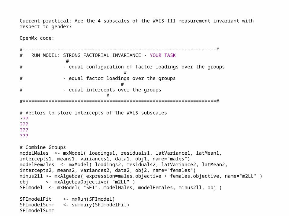
Current practical: Are the 4 subscales of the WAIS-III measurement invariant with respect to gender?
OpenMx code:
#===================================================================## RUN MODEL: STRONG FACTORIAL INVARIANCE - YOUR TASK ## - equal configuration of factor loadings over the groups
## - equal factor loadings over the groups ## - equal intercepts over the groups # #===================================================================#
# Vectors to store intercepts of the WAIS subscales????????????
# Combine GroupsmodelMales <- mxModel( loadings1, residuals1, latVariance1, latMean1, intercepts1, means1, variances1, data1, obj1, name="males")modelFemales <- mxModel( loadings2, residuals2, latVariance2, latMean2,intercepts2, means2, variances2, data2, obj2, name="females")minus2ll <- mxAlgebra( expression=males.objective + females.objective, name="m2LL" )obj <- mxAlgebraObjective( "m2LL" )SFImodel <- mxModel( "SFI", modelMales, modelFemales, minus2ll, obj )
SFImodelFit <- mxRun(SFImodel)SFImodelSumm <- summary(SFImodelFit)SFImodelSumm
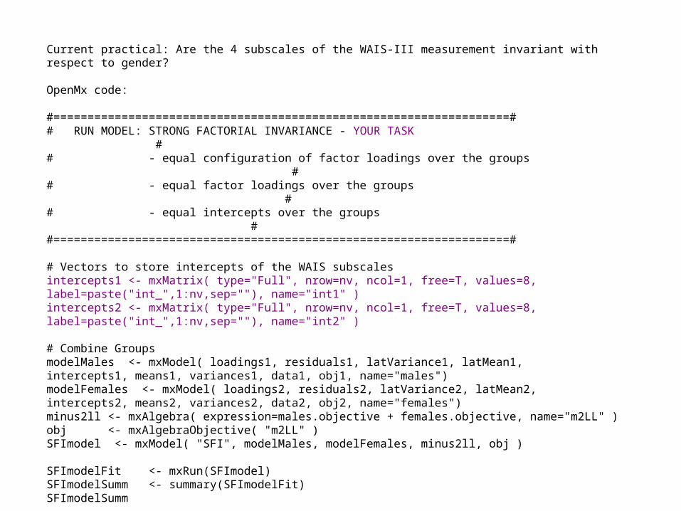
Current practical: Are the 4 subscales of the WAIS-III measurement invariant with respect to gender?
OpenMx code:
#===================================================================## RUN MODEL: STRONG FACTORIAL INVARIANCE - YOUR TASK ## - equal configuration of factor loadings over the groups
## - equal factor loadings over the groups ## - equal intercepts over the groups # #===================================================================#
# Vectors to store intercepts of the WAIS subscalesintercepts1 <- mxMatrix( type="Full", nrow=nv, ncol=1, free=T, values=8,label=paste("int_",1:nv,sep=""), name="int1" )intercepts2 <- mxMatrix( type="Full", nrow=nv, ncol=1, free=T, values=8,label=paste("int_",1:nv,sep=""), name="int2" )
# Combine GroupsmodelMales <- mxModel( loadings1, residuals1, latVariance1, latMean1, intercepts1, means1, variances1, data1, obj1, name="males")modelFemales <- mxModel( loadings2, residuals2, latVariance2, latMean2,intercepts2, means2, variances2, data2, obj2, name="females")minus2ll <- mxAlgebra( expression=males.objective + females.objective, name="m2LL" )obj <- mxAlgebraObjective( "m2LL" )SFImodel <- mxModel( "SFI", modelMales, modelFemales, minus2ll, obj )
SFImodelFit <- mxRun(SFImodel)SFImodelSumm <- summary(SFImodelFit)SFImodelSumm
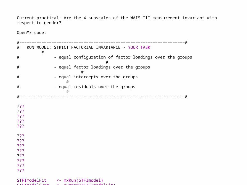
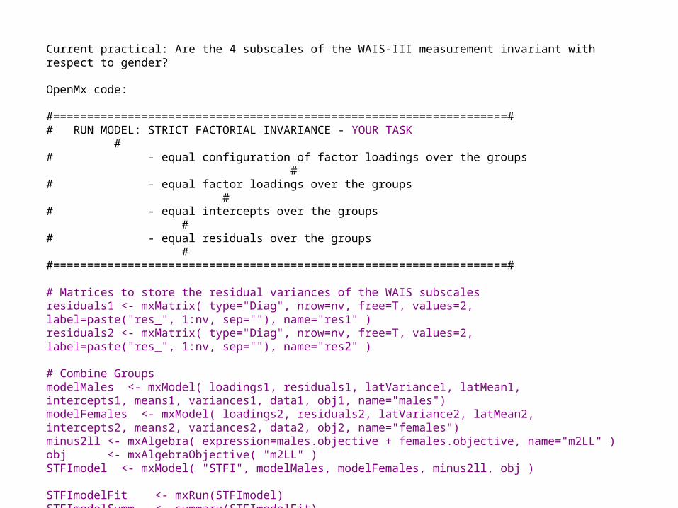
Current practical: Are the 4 subscales of the WAIS-III measurement invariant with respect to gender?
OpenMx code:
#===================================================================## RUN MODEL: STRICT FACTORIAL INVARIANCE - YOUR TASK ## - equal configuration of factor loadings over the groups
## - equal factor loadings over the groups
## - equal intercepts over the groups ## - equal residuals over the groups ##===================================================================#
???????????????
????????????????????????
STFImodelFit <- mxRun(STFImodel)STFImodelSumm <- summary(STFImodelFit)STFImodelSumm
Current practical: Are the 4 subscales of the WAIS-III measurement invariant with respect to gender?
OpenMx code:
#===================================================================## RUN MODEL: STRICT FACTORIAL INVARIANCE - YOUR TASK ## - equal configuration of factor loadings over the groups
## - equal factor loadings over the groups
## - equal intercepts over the groups ## - equal residuals over the groups ##===================================================================#
# Matrices to store the residual variances of the WAIS subscalesresiduals1 <- mxMatrix( type="Diag", nrow=nv, free=T, values=2, label=paste("res_", 1:nv, sep=""), name="res1" )residuals2 <- mxMatrix( type="Diag", nrow=nv, free=T, values=2, label=paste("res_", 1:nv, sep=""), name="res2" )
# Combine GroupsmodelMales <- mxModel( loadings1, residuals1, latVariance1, latMean1, intercepts1, means1, variances1, data1, obj1, name="males")modelFemales <- mxModel( loadings2, residuals2, latVariance2, latMean2,intercepts2, means2, variances2, data2, obj2, name="females")minus2ll <- mxAlgebra( expression=males.objective + females.objective, name="m2LL" )obj <- mxAlgebraObjective( "m2LL" )STFImodel <- mxModel( "STFI", modelMales, modelFemales, minus2ll, obj )
STFImodelFit <- mxRun(STFImodel)STFImodelSumm <- summary(STFImodelFit)STFImodelSumm
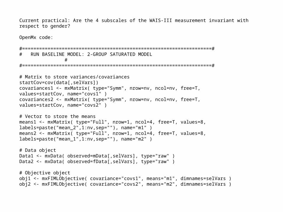
Current practical: Are the 4 subscales of the WAIS-III measurement invariant with respect to gender?
OpenMx code:
#===================================================================## RUN BASELINE MODEL: 2-GROUP SATURATED MODEL ##===================================================================#
# Matrix to store variances/covariancesstartCov=cov(data[,selVars])covariances1 <- mxMatrix( type="Symm", nrow=nv, ncol=nv, free=T, values=startCov, name="covs1" )covariances2 <- mxMatrix( type="Symm", nrow=nv, ncol=nv, free=T, values=startCov, name="covs2" )
# Vector to store the meansmeans1 <- mxMatrix( type="Full", nrow=1, ncol=4, free=T, values=8,labels=paste("mean_2",1:nv,sep=""), name="m1" )means2 <- mxMatrix( type="Full", nrow=1, ncol=4, free=T, values=8,labels=paste("mean_1",1:nv,sep=""), name="m2" )
# Data objectData1 <- mxData( observed=mData[,selVars], type="raw" )Data2 <- mxData( observed=fData[,selVars], type="raw" )
# Objective objectobj1 <- mxFIMLObjective( covariance="covs1", means="m1", dimnames=selVars )obj2 <- mxFIMLObjective( covariance="covs2", means="m2", dimnames=selVars )
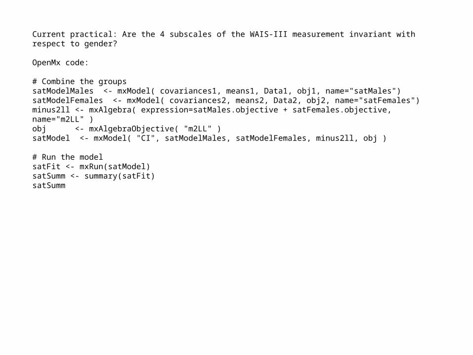
Current practical: Are the 4 subscales of the WAIS-III measurement invariant with respect to gender?
OpenMx code:
# Combine the groupssatModelMales <- mxModel( covariances1, means1, Data1, obj1, name="satMales")satModelFemales <- mxModel( covariances2, means2, Data2, obj2, name="satFemales")minus2ll <- mxAlgebra( expression=satMales.objective + satFemales.objective, name="m2LL" )obj <- mxAlgebraObjective( "m2LL" )satModel <- mxModel( "CI", satModelMales, satModelFemales, minus2ll, obj )
# Run the modelsatFit <- mxRun(satModel)satSumm <- summary(satFit)satSumm
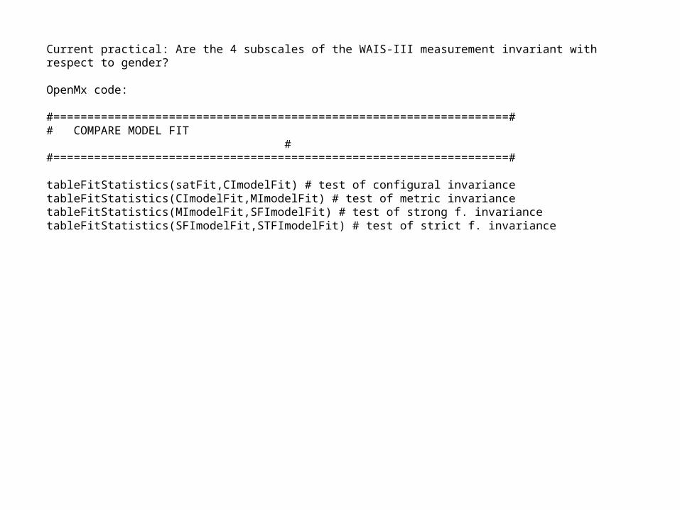
Current practical: Are the 4 subscales of the WAIS-III measurement invariant with respect to gender?
OpenMx code:
#===================================================================## COMPARE MODEL FIT # #===================================================================#
tableFitStatistics(satFit,CImodelFit) # test of configural invariancetableFitStatistics(CImodelFit,MImodelFit) # test of metric invariancetableFitStatistics(MImodelFit,SFImodelFit) # test of strong f. invariancetableFitStatistics(SFImodelFit,STFImodelFit) # test of strict f. invariance
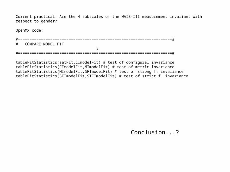
Current practical: Are the 4 subscales of the WAIS-III measurement invariant with respect to gender?
OpenMx code:
#===================================================================## COMPARE MODEL FIT ##===================================================================#
tableFitStatistics(satFit,CImodelFit) # test of configural invariancetableFitStatistics(CImodelFit,MImodelFit) # test of metric invariancetableFitStatistics(MImodelFit,SFImodelFit) # test of strong f. invariancetableFitStatistics(SFImodelFit,STFImodelFit) # test of strict f. invariance
Conclusion...?