faultlocationinpowerdistribution ... · faultlocationinpowerdistribution...
TRANSCRIPT

Universidade de São Paulo–USPEscola Politécnica
Laiz de Carvalho Souto
Fault location in power distributionnetworks with distributed generation
São Paulo2016


Laiz de Carvalho Souto
Fault location in power distributionnetworks with distributed generation
Master Dissertation presented at Escola Politécnica forthe degree of Master of Science.Dissertação de mestrado apresentada à Escola Politéc-nica para a obtenção do título de Mestre em Ciências.
Concentration area: Electric Power SystemsÁrea de concentração: Sistemas Elétricos de Potência
Supervisor: Prof. Dr. Giovanni Manassero Junior
São Paulo2016

Este exemplar foi revisado e corrigido em relação à versão original, sob responsabilidade única do autor e com a anuência de seu orientador.
São Paulo, ______ de ____________________ de __________
Assinatura do autor: ________________________
Assinatura do orientador: ________________________
Catalogação-na-publicação
Souto, Laiz Fault location in power distribution networks with distributed generation /L. Souto -- versão corr. -- São Paulo, 2016. 114 p.
Dissertação (Mestrado) - Escola Politécnica da Universidade de SãoPaulo. Departamento de Engenharia de Energia e Automação Elétricas.
1.Proteção de sistemas elétricos 2.Redes de distribuição de energiaelétrica 3.Energia elétrica (geração distribuída) 4.Sistemas elétricos depotência (automação) I.Universidade de São Paulo. Escola Politécnica.Departamento de Engenharia de Energia e Automação Elétricas II.t.
THE TOTAL OR PARTIAL REPRODUCTION OF THIS WORK IS AUTHORISEDON ANY CONVENTIONAL OR ELECTRONIC MEANS FOR STUDY AND RESEARCHPURPOSES, AS LONG AS CITED THE SOURCE.
AUTORIZO A REPRODUÇÃO TOTAL OU PARCIAL DESTE TRABALHO, PORQUALQUER MEIO CONVENCIONAL OU ELETRÔNICO, PARA FINS DE ESTUDOE PESQUISA, DESDE QUE CITADA A FONTE.

To all those interested in fault location in electric power systems


Acknowledgements
I would like to acknowledge everyone who assisted me during my graduate programat the Escola Politécnica da Universidade de São Paulo (POLI-USP) and during my visitand exchange study at the Royal Institute of Technology (KTH). First and foremost,I would like to thank Prof. Giovanni Manassero Junior, my supervisor at POLI-USP,for his guidance, support and patience throughout my years as a graduate student, andResearcher Nathaniel Taylor, my supervisor at KTH, for his guidance and personal timethat I truly appreciated.
Special thanks are given to Prof. Silvio Giuseppe Di Santo, for his support with thefault location algorithms; to Prof. Hernán Preito Schmidt, for his indication to join thisgraduate program; and to Prof. Carlos Eduardo de Moraes Pereira, Prof. Milana dosSantos, Prof. Eduardo Cesar Senger, Prof. Eduardo Lorenzetti Pellini, Prof. RenatoMachado Monaro and Prof. Ivan Eduardo Chabu, for their clarifications.
On the top of that, I am grateful to TOSHIBA Corporation and FAPESP for fun-ding this research project (Grant 2014/Ms-01, TOSHIBA Scholarship Program, processnumber 2013/23117-0, Fundação de Amparo à Pesquisa do Estado de São Paulo).
Last, but not least, I would like to thank my family and all my friends and colleaguesfor their unconditional support throughout these years.


"There are no unlockable doorsThere are no unwinnable wars
There are no unrightable wrongsor unsingable songs"
(Ozzy Osbourne)


Abstract
Souto, Laiz Fault location in power distribution networks with distributedgeneration. 114 p. Master Dissertation – Polytechnic School, University of São Paulo,2016.
This research presents the development and implementation of fault location algo-rithms in power distribution networks with distributed generation units installed alongtheir feeders. The proposed algorithms are capable of locating the fault based on voltageand current signals recorded by intelligent electronic devices installed at the end of thefeeder sections, information to compute the loads connected to these feeders and theirelectric characteristics, and the operating status of the network. In addition, this workpresents the study of analytical models of distributed generation and load technologiesthat could contribute to the performance of the proposed fault location algorithms. Thevalidation of the algorithms was based on computer simulations using network modelsimplemented in ATP, whereas the algorithms were implemented in MATLAB.
Keywords: power system protection, power system automation, fault location, distribu-ted generation.


Resumo
Souto, Laiz Localização de faltas em redes elétricas de distribuição com apresença de unidades de geração distribuída. 114 p. Dissertação de mestrado –Escola Politécnica, Universidade de São Paulo, 2016.
Esta pesquisa apresenta o desenvolvimento e a implementação de algoritmos paralocalização de faltas em redes primárias de distribuição de energia elétrica que possuemunidades de geração distribuída conectadas ao longo dos seus alimentadores. Esses algorit-mos são capazes de efetuar a localização de faltas utilizando registros dos sinais de tensõese correntes realizados por dispositivos eletrônicos inteligentes, instalados nas saídas dosalimentadores de distribuição, além de informações que permitam determinar os valoresdas cargas conectadas nesses alimentadores, características elétricas, e o estado operativoda rede de distribuição. Ademais, este trabalho apresenta o estudo de modelos analíticosde unidades de geração distribuída e de cargas que poderiam contribuir positivamente como desempenho dos algoritmos propostos. A validação dos algoritmos foi realizada atravésde simulações computacionais, utilizando modelos de rede implementados em ATP e osalgoritmos foram implementados em MATLAB.
Palavras-chave: proteção de sistemas elétricos, automação de sistemas elétricos, locali-zação de faltas, geração distribuída.


List of illustrations
Figure 1 Typical distribution feeder . . . . . . . . . . . . . . . . . . . . . . . . . 27Figure 2 Block diagram of an automated fault location system . . . . . . . . . . 29
Figure 3 Three-phase full diode bridge rectifier . . . . . . . . . . . . . . . . . . . 38Figure 4 Three-phase 12-diode bridge rectifier with transformers . . . . . . . . . 38Figure 5 Schematic of a fixed-speed wind turbine . . . . . . . . . . . . . . . . . 42Figure 6 Induction generator third-order model neglecting stator transients . . . 45Figure 7 Equivalent circuit of the induction generator ninth-order model, reac-
tive power compensating capacitor and grid . . . . . . . . . . . . . . . 45Figure 8 Schematic of a wind turbine with variable external resistance . . . . . . 48Figure 9 Schematic of a DFIG wind turbine . . . . . . . . . . . . . . . . . . . . 49Figure 10 Schematic of a wind turbine with full-load power converter . . . . . . . 57Figure 11 Single-line diagram of a detailed wind farm model with 12 wind turbines 60Figure 12 Equivalent electrical circuit of a single photovoltaic cell . . . . . . . . . 65Figure 13 Equivalent electrical circuit of a fuel cell . . . . . . . . . . . . . . . . . 69Figure 14 Equivalent electrical circuit of a gas micro turbine . . . . . . . . . . . . 70Figure 15 WECC Composite Load Model . . . . . . . . . . . . . . . . . . . . . . 72
Figure 16 Radial distribution feeder - Algorithm 1 . . . . . . . . . . . . . . . . . 78Figure 17 Block diagram - Scenario 1 . . . . . . . . . . . . . . . . . . . . . . . . . 80Figure 18 Equivalent sources at the investigated line section . . . . . . . . . . . . 82Figure 19 Fault admittance at the investigated line section . . . . . . . . . . . . . 83Figure 20 Fault current injection at the investigated line section . . . . . . . . . . 84Figure 21 Radial distribution feeder - Algorithm 2 . . . . . . . . . . . . . . . . . 88Figure 22 Block diagram - Scenario 2 . . . . . . . . . . . . . . . . . . . . . . . . . 88Figure 23 Equivalent admittance in the two-port network model with source at
one end . . . . . . . . . . . . . . . . . . . . . . . . . . . . . . . . . . . 90Figure 24 Two-port network model with source at two ends - Situation II . . . . . 92Figure 25 Block diagram - Scenario 3 . . . . . . . . . . . . . . . . . . . . . . . . . 95

Figure 26 Distribution pole . . . . . . . . . . . . . . . . . . . . . . . . . . . . . . 99Figure 27 Histogram of correct line sections identification . . . . . . . . . . . . . 106

List of tables
Table 1 Comparison between distribution categories . . . . . . . . . . . . . . . . 28Table 2 Comparison between fault location techniques with DFRs installed at
different locations . . . . . . . . . . . . . . . . . . . . . . . . . . . . . . 31
Table 3 Typical fault levels of power-converter-interfaced DGs . . . . . . . . . . 40
Table 4 Short-circuit rating . . . . . . . . . . . . . . . . . . . . . . . . . . . . . 99Table 5 Short-circuit impedance data . . . . . . . . . . . . . . . . . . . . . . . . 99Table 6 Simulation data . . . . . . . . . . . . . . . . . . . . . . . . . . . . . . . 100Table 7 Fault location errors for the algoritm 1 . . . . . . . . . . . . . . . . . . . 101Table 8 Points of the applied faults . . . . . . . . . . . . . . . . . . . . . . . . . 101Table 9 Fault location errors for the algorithm 2 . . . . . . . . . . . . . . . . . . 102Table 10 Fault location errors for the algorithm 3 . . . . . . . . . . . . . . . . . . 102Table 11 Fault location errors with errors in the equivalent sources estimations . 103Table 12 Fault location errors with errors in the load estimation . . . . . . . . . . 104Table 13 Fault location errors with errors in the line section parameters . . . . . 105Table 14 Fault location errors with errors in the phasor quantities . . . . . . . . . 106

Acronyms
AC alternate current
A/D analogical/digital
ATP Alternative Transient Program
CT Instrument Current Transformer
DC direct current
DG distributed generation
DFIG Doubly-Fed Induction Generator
DFR digital fault recorder
DKE Deutsche Kommission Elektrotechnik
d-q direct-quadrature
EMF electromotive force
GFRT Grid-Fault Ride-Through
GSC grid-side converter
HV High Voltage
IEC International Electrotechnical Comission
IED Intelligent Electronic Device
IEEE Institute of Electrical and Electronic Engineers
IG Induction Generator
IGBT Insulated-gate bipolar transistor

I-V current-voltage
MATLAB Matrix Laboratory
MCFC Molten carbonate fuel cell
MOV Metal Oxide Varistor
MPPT Maximum Power Point Tracking
MSC machine-side converter
MV Medium Voltage
PEMFC Polymer electrolyte membrane fuel cell
PV Photovoltaic
PMSG Permanent Magnet Synchronous Generator
PMU Phasor Measurement Unit
p.u. per unit
PWM Pulse Width Modulation
RMS Root Mean Square
RSC rotor-side converter
SCIG Squirrel-Cage Induction Generator
SOFC Solid oxide fuel cell
STATCOM Static Converter
VFD variable frequency drive
VSC Voltage Source Converter
VT Instrument Voltage Transformer
WECC Wisconsin Energy Conservation Corporation
WRIG Wound Rotor Induction Generator
WTG Wind Turbine Generator
Table of contents
1 Introduction 231.1 General . . . . . . . . . . . . . . . . . . . . . . . . . . . . . . . . . . . . . 231.2 Motivations . . . . . . . . . . . . . . . . . . . . . . . . . . . . . . . . . . . 231.3 Objectives and outlines . . . . . . . . . . . . . . . . . . . . . . . . . . . . 241.4 Contributions . . . . . . . . . . . . . . . . . . . . . . . . . . . . . . . . . 251.5 Publications . . . . . . . . . . . . . . . . . . . . . . . . . . . . . . . . . . 25
2 Review of Fault Location Techniques 262.1 Basic principles . . . . . . . . . . . . . . . . . . . . . . . . . . . . . . . . 262.2 Distribution networks . . . . . . . . . . . . . . . . . . . . . . . . . . . . . 262.3 Typical approach of an automated fault location system . . . . . . . . . . 282.4 Errors of fault location . . . . . . . . . . . . . . . . . . . . . . . . . . . . 282.5 Fault location in power distribution lines . . . . . . . . . . . . . . . . . . 30
2.5.1 Accuracy issues . . . . . . . . . . . . . . . . . . . . . . . . . . . . 312.5.2 Conventional methods . . . . . . . . . . . . . . . . . . . . . . . . . 332.5.3 Fault location in distribution networks without DG units . . . . . 342.5.4 Fault location in distribution networks with DG units . . . . . . . 35
3 Review of modelling distributed generation and load technologies 373.1 Power Conditioning Units . . . . . . . . . . . . . . . . . . . . . . . . . . . 37
3.1.1 AC-DC rectifiers . . . . . . . . . . . . . . . . . . . . . . . . . . . . 373.1.2 DC-DC converters . . . . . . . . . . . . . . . . . . . . . . . . . . . 393.1.3 DC-AC inverters . . . . . . . . . . . . . . . . . . . . . . . . . . . . 393.1.4 Impact of power-converter-interfaced DGs on short-circuit levels . 39
3.2 Fault Behaviour of Wind Turbines . . . . . . . . . . . . . . . . . . . . . . 403.2.1 Wind turbine concepts . . . . . . . . . . . . . . . . . . . . . . . . 403.2.2 Wind farms . . . . . . . . . . . . . . . . . . . . . . . . . . . . . . 593.2.3 Grid-fault ride-through requirements . . . . . . . . . . . . . . . . . 62

3.3 Fault Behaviour of Photovoltaic Systems . . . . . . . . . . . . . . . . . . 633.3.1 Basic concepts of photovoltaic systems . . . . . . . . . . . . . . . . 633.3.2 Grid requirements for response to abnormal conditions . . . . . . . 643.3.3 Modelling photovoltaic systems . . . . . . . . . . . . . . . . . . . . 64
3.4 Fault Behaviour of Fuel Cells . . . . . . . . . . . . . . . . . . . . . . . . . 673.4.1 Basic concepts . . . . . . . . . . . . . . . . . . . . . . . . . . . . . 673.4.2 Dynamic models for fuel cells . . . . . . . . . . . . . . . . . . . . . 68
3.5 Fault Behaviour of Gas Micro-turbines . . . . . . . . . . . . . . . . . . . . 693.5.1 Basic concepts of gas micro-turbines . . . . . . . . . . . . . . . . . 693.5.2 Dynamic models for gas micro-turbines . . . . . . . . . . . . . . . 70
3.6 Fault Behaviour of Loads . . . . . . . . . . . . . . . . . . . . . . . . . . . 703.6.1 Previous attempts on load modelling . . . . . . . . . . . . . . . . . 713.6.2 Validation studies . . . . . . . . . . . . . . . . . . . . . . . . . . . 76
4 The Proposed Fault Location Algorithms 784.1 General . . . . . . . . . . . . . . . . . . . . . . . . . . . . . . . . . . . . . 784.2 Proposed fault location algorithm 1 . . . . . . . . . . . . . . . . . . . . . 79
4.2.1 Estimation of the equivalent sources and load impedances . . . . . 794.2.2 Estimation of the equivalent circuit of the investigated line section 814.2.3 Estimation of the current at the fault location . . . . . . . . . . . 834.2.4 Estimation of the post-fault voltages and currents phasor quanti-
ties at the substation . . . . . . . . . . . . . . . . . . . . . . . . . 844.2.5 Optimization tool . . . . . . . . . . . . . . . . . . . . . . . . . . . 86
4.3 Proposed fault location algorithm 2 . . . . . . . . . . . . . . . . . . . . . 874.3.1 Two-port network representation . . . . . . . . . . . . . . . . . . . 894.3.2 Procedures . . . . . . . . . . . . . . . . . . . . . . . . . . . . . . . 904.3.3 Comparison between measured and calculated current phasors . . 944.3.4 Optimization tool . . . . . . . . . . . . . . . . . . . . . . . . . . . 94
4.4 Proposed fault location algorithm 3 . . . . . . . . . . . . . . . . . . . . . 944.4.1 Estimation of the equivalent sources and load impedances . . . . . 954.4.2 Estimation of the equivalent two-port network representation of
the investigated line section . . . . . . . . . . . . . . . . . . . . . . 964.4.3 Estimation of the post-fault voltages and currents phasor quanti-
ties at the substation . . . . . . . . . . . . . . . . . . . . . . . . . 964.4.4 Optimization tool . . . . . . . . . . . . . . . . . . . . . . . . . . . 97
4.5 Evaluation of the fault location algorithms . . . . . . . . . . . . . . . . . 97
5 Simulations and Results 985.1 General . . . . . . . . . . . . . . . . . . . . . . . . . . . . . . . . . . . . . 985.2 Simulation premises . . . . . . . . . . . . . . . . . . . . . . . . . . . . . . 98

5.3 Simulation results . . . . . . . . . . . . . . . . . . . . . . . . . . . . . . . 1005.3.1 Algorithm 1 . . . . . . . . . . . . . . . . . . . . . . . . . . . . . . 1005.3.2 Algorithm 2 . . . . . . . . . . . . . . . . . . . . . . . . . . . . . . 1015.3.3 Algorithm 3 . . . . . . . . . . . . . . . . . . . . . . . . . . . . . . 1015.3.4 Sensitivity analysis . . . . . . . . . . . . . . . . . . . . . . . . . . 1025.3.5 Histogram . . . . . . . . . . . . . . . . . . . . . . . . . . . . . . . 106
Conclusion 108Conclusion . . . . . . . . . . . . . . . . . . . . . . . . . . . . . . . . . . . . . . 108Further Perspectives . . . . . . . . . . . . . . . . . . . . . . . . . . . . . . . . . 108
References 109


23
Chapter 1Introduction
1.1 General
The presence of distributed generation (DG) in power distribution networks may bringimpacts to conventional protection and automation systems, because of irregularity inenergy availability and power quality and stability issues, such as momentary variationsin voltage levels and increase in harmonic content and short-circuit levels. As a result,traditional fault location algorithms are no longer valid in these conditions (GHORBANI;
CHOUDHRY; FELIACHI, 2013; OROZCO-HENAO; MORA-FLOREZ; PEREZ-LONDONO, 2012;HAGH; HOSSEINI; ASGARIFAR, 2012; WU et al., 2011).
Fault location in power distribution networks plays a critical role to reduce supplyinterruption rates and increase power quality to consumers. Therefore, it is of paramountimportance to develop accurate fault location procedures that takes into account these newconditions, and also apply models that properly represent the DG and load technologiesso that the fault location procedures present a satisfactory degree of accuracy.
This research project fits into this context and presents fault location algorithms inpower distribution networks with the presence of DG. The text is structured as follows:Chapter 2 describes the accuracy issues of the fault location techniques in use, Chap-ter 3 presents the DG and load technologies commonly used and their behaviour undershort-circuits (Section 3.2 to Section 3.6); afterwards, Chapter 4 presents the proposedfault location algorithms, taking into consideration distinct scenarios; to conclude, detailsof the simulations are presented in Chapter 5, followed by the conclusions and futureperspectives.
1.2 Motivations
The analysis of the dynamic behaviour of electric power systems requires equivalentmodels that represent the phenomena of interest together with accurate parameters toensure replication of reality. The choice of models relies on knowledge of the actual

24 Chapter 1. Introduction
system composition and the phenomena in study, whereas the estimation of parametersminimizes the differences between the measured and simulated behaviour. Different modelstructures may lead to different parameter values, as the estimations tend to compensatefor poorly-modelled effects.
The model complexity and the aim of the investigations have to comply with eachother. Hence, representation of a given component present in the construction has apurpose with respect to the target of the investigations. On the one hand, over-simplifiedmodels may not represent the complexity of a given component accurately; on the otherhand, over-detailed models are more difficult to describe, produce slower simulations andunnecessary outputs that may confuse the interpretation of results. Therefore, genericmodels may be parametrised in such a way that a wide range of components can berepresented reasonably well.
Modelling power distribution systems with DG is a difficult task due to their inherentcomplexity. The technologies in use present different behaviours under abnormal condi-tions and often require static converters to be connected to the alternate current (AC)grid. As a result, the system behaviour is conditioned by static converters and DG unitsduring grid disturbances. In a recent past, the influence of these technologies on theoverall operating conditions was negligible due to their low penetration levels; consequen-tly, simplified models, such as the constant power supply, were adopted without reducingthe accuracy of electrical studies. Recently, their increasing penetration level has re-quested the development of appropriate models to evaluate system performance duringshort-circuits.
In turn, modelling loads is challenging because most of the utilities have no detailedinformation about the characteristics of what is connected to the grid, although it isimportant for various electrical studies and particularly for fault location. Some faultlocation algorithms apply simplified load models or ignore the load current, which maylead to inaccurate solutions. Correct estimations of the load current contribution mayimprove the accuracy of fault location, regardless of their non-deterministic behaviour.Some techniques have good precision for load estimation, such as daily load curves andoptimization methods.
To conclude, it is necessary to use accurate analytical models that represent the behavi-our of the DGs, loads and power converters when the grid is subjected to a fault condition,so that the fault location system can indicate the fault position accurately.
1.3 Objectives and outlines
The main goals of this thesis are summarized as follows:– Evaluate the state of the art of fault location techniques;
– Evaluate distinct fault location procedures;

– Describe the short-circuit current contribution of distributed generation technologiescommonly used, notably wind turbines, photovoltaic cells, fuel cells and gas micro-turbines;
– Describe the impact of loads on the short-circuit currents;
– Describe the influence of power conditioning units on the short-circuit current contri-bution of distributed energy resources and loads;
– Study and develop fault location algorithms in power distribution networks with dis-tributed energy resources installed along the feeders;
– Validate the proposed fault location algorithms implemented in Matrix Laboratory(MATLAB) through study cases simulated in Alternative Transient Program (ATP).
1.4 Contributions
This thesis aims to contribute for the development and consolidation of fault locationalgoritms in primary distribution networks with DGs installed along the feeders, as wellas to proceed with simulations and tests to validate them. In addition, this projectaims at studying analytical models of distributed energy resources and loads during griddisturbances for the same purposes. As a consequence, it is expected that this researchprovides useful information on the understanding of this subject.
1.5 Publications
a) Souto L. C., Manassero G. Jr., Di Santo S. G., Fault Location in DistributionFeeders with Distributed Generation, 2016 Clemson University Power SystemsConference, Clemson, 08-11 March 2016.
b) Souto L. C., Manassero G. Jr., Di Santo S. G., Heuristic Method for Fault Loca-tion in Distribution Feeders with the Presence of Distributed Generation, IEEETransactions on Smart Grid (submitted).
* * *

Chapter 2Review of Fault Location Techniques
2.1 Basic principles
Power transmission and distribution systems are susceptible to short-circuits that candamage them and their connected equipment. Protection schemes are expected to operatein order to clear the fault, by opening the circuit breakers that connect the damaged lineto the healthy part of the network. Reclosing schemes are used to bring the line backin operation after the fault is cleared. Temporary faults are cleared in such a way thatthe power supply continuity is not affected permanently. Conversely, if all the reclosingattempts fail, the fault will be assumed permanent, the circuit breaker associated to theprotective relaying equipment will remain open to de-energize the faulted sections.
Faults in power distribution networks are often located through physical indicationsand field methods such as restoration through switching or recloser operation, indicationthrough fuse and fault-locator operation, downed wires, customer calls and maps, relaytargets and direct current (DC) thumping of underground circuits. However, high accu-racy is needed in determining the fault location for efficient dispatch of repair crews, oftensearching in bad weather conditions or at places that are difficult to reach.
The accuracy of a given fault location technique may be affected by several aspects,such as the network elements and the analytical models applied. In turn, the limitationsof a given procedure may influence the level of details required to represent adequatelysuch factors. If a particular factor affects fault-location accuracy, then the means of itselimination or minimization have to be considered. Thus, it is important to understandhow a particular factor and the accuracy of a given fault location technique may affecteach other, so that the means of minimization of errors can be considered.
2.2 Distribution networks
The fault location algorithms developed within this work are intended to power distri-bution networks. Thereby, a brief explanation about the main characteristics of a typical

2.2. Distribution networks 27
+
10 3020IS.
VS.
4050
90
60 80
70
100
110
120
130
VST.
Sl,20
_Sl,30
_
Sl,90
_
Sl,100
_
Sl,110
_
Sl,50
_Sl,40
_
Sl,70
_
Sl,60
_
Sl,120
_
Sl,130
_
Sl,80
_
Figure 1 – Typical distribution feeder
Source: the author
distribution network is provided in the next paragraphs.Primary distribution feeders usually have a main line section (line section 10-50) that
leaves the substation and is connected to a number of lateral branches (branches 30-90,40-100, 100-110, 20-60, 60-70, 60-80, 60-120 and 120-130), as illustrated in Figure 1.Intelligent Electronic Device (IED)s installed only at the substation bus (bus 10 in Fi-gure 1) or at the substation bus and connection points of DGs (buses 50, 70, 110 and130 in Figure 1) are responsible for protecting the main line section of the feeder andproviding backup protection to the fuses installed at the lateral branches.
Typical distribution feeders are radial, with different configurations, lines and cablesalong them; therefore, the relation between the sections’ impedances and the fault distanceis non-linear. Moreover, faults at different locations may result in the same voltage andcurrent signals recorded at the substation. Furthermore, the current measured at thesubstation during an overcurrent event may include load currents at each bus and it isvirtually impossible to estimate them precisely.
The connection of DGs changes distribution network topology from single-power tomulti-power. Consequently, traditional fault location algorithms are no longer applicableunder such conditions. High penetration levels of DG will have unfavorable impact onthese methods, depending on the number, location and injected current of DG.
For clarification purposes, the differences between radial and network distributionschemes are summarised in Table 1.

28 Chapter 2. Review of Fault Location Techniques
Table 1 – Comparison between distribution categories
Radial distribution Network distribution
Characteristics– independent feeders branch out radi-
ally from a common supply source
– circuits with multiple branches andservice taps
– areas with high load density and ma-ximum reliability requirements
Parameters
– cable length– presence of transformers in a loop– short and open circuits– neutral corrosion
– overall circuit length and number ofbranches
– lumped cable system capacitance– insulation type– fault resistance– transformer primary connection
Source: IEEE-Std.1234-2007 (2007) (adapted)
2.3 Typical approach of an automated fault locationsystem
An automated fault location system requests IEDs installed at the distribution network,as well as communication channels to allow the exchange of information between the IEDsand the system operator.
The IEDs are responsible for recording the voltage and current signals at a few points(usually at the substation bus and sometimes at the connection points of the DG unitsand other points of common coupling) at a given sample rate. The recorded quantities aresent via communication channels to the system fault location system, which processes thereceived information and calculates: the pre-fault, fault and post-fault phasor quantities;and the fault type and phases involved. Than it uses these information together with theelectrical parameters and topology of the distribution network stored in a database toidentify the point of fault. After the system response, the repair crew can be dispatchedfast and efficiently.
The operation processes of a typical automated fault location system are schematisedin Figure 2, and this work focuses on the development of fault location algorithms thatcomprise the automated fault location system.
2.4 Errors of fault location
Various factors may impact the accuracy of fault location and must be taken intoaccount (SAHA; IZYKOWSKI; ROSOLOWSKI, 2010; GILBERT; MORRISON, 1997; EINARS-
SON, 2005; IEEE-C37.114-WG, 2015). Overall, accuracy issues may be grouped in threecategories, as follows:

2.4. Errors of fault location 29
Pre-fault,vfaultvandvpost-faultvquantities
Faultvlocationvalgorithmv
START
Faultvdetection
Identificationvofvthevfaultvtypevandvfaultedvphases
Readingvofvthevfilesvwithvinformationvaboutvthevsampledvvoltagesvandvcurrents
voltagesvandvcurrentsv
IEDs
andvsamplingvofvReal-timevmonitoringv
invthevoperatingvcentrevProcessingvofvthevfaultvfilesv
Figure 2 – Block diagram of an automated fault location system
Source: the author
a) Software-related issues: include basic problems in numerical computation, such asrounding, cancellation, recursion, floating-point precision, illegal data and illegalconversion between data types, and errors in software implementation (EINARSSON,2005). The issues within this category may affect measurement and parameterestimations.
b) Measurement-related issues: include transient- and steady-state errors of InstrumentVoltage Transformer (VT)s and Instrument Current Transformer (CT)s includingunfaithful reproduction of the primary signals due to their limited bandwidth andpossibility of CT saturation, time and frequency response of voltage and currentmeasurement chains, accuracy of analogical/digital (A/D) conversion in terms ofsampling frequency and bit resolution.
c) Parameter-related issues: comprehends fault resistance, including presence of anarc; inaccuracy in providing impedance data for the overhead line, due to the lackof information about the geometry and total length of its conductors, especiallyfor the zero-sequence impedance, which is affected by the soil resistivity (variableunder the whole line route and dependent on the weather conditions), as well as forthe source impedances (in case they are involved in the fault location algorithm);strength of equivalent sources behind the line terminals; improper line model, gi-ven that long lines on high voltage levels may exhibit considerable capacitance andsignificant charging current and have to be considered within the algorithm; lineimbalance due to lack of transposition, provided that untransposed lines are repre-sented as being transposed; presence and status of series and shunt devices in theline and substation nodes, such as banks of series capacitors equipped with Metal
30 Chapter 2. Review of Fault Location Techniques
Oxide Varistor (MOV)s. Such uncertainties may result in inaccurate compensa-tion for the reactance effect in the case of fault location algorithms using one-endmeasurements, as well as for the mutual effects on the zero-sequence components,if the current required to compensate the mutual coupling is unavailable.
2.5 Fault location in power distribution lines
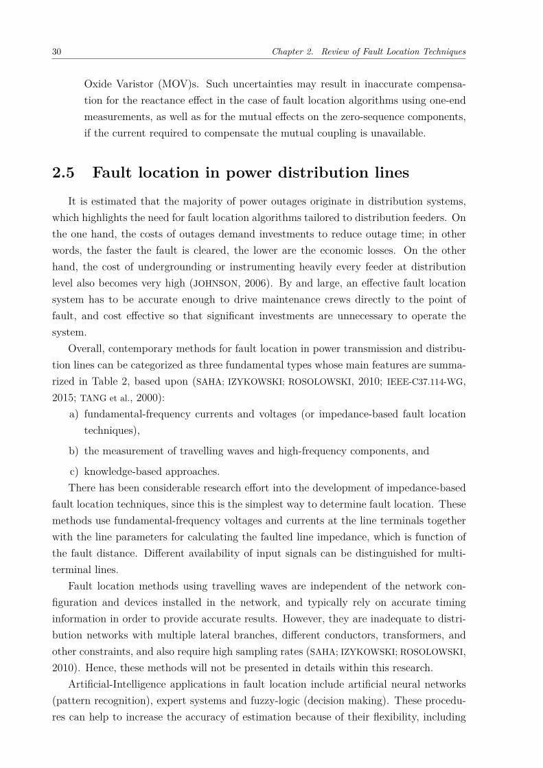
It is estimated that the majority of power outages originate in distribution systems,which highlights the need for fault location algorithms tailored to distribution feeders. Onthe one hand, the costs of outages demand investments to reduce outage time; in otherwords, the faster the fault is cleared, the lower are the economic losses. On the otherhand, the cost of undergrounding or instrumenting heavily every feeder at distributionlevel also becomes very high (JOHNSON, 2006). By and large, an effective fault locationsystem has to be accurate enough to drive maintenance crews directly to the point offault, and cost effective so that significant investments are unnecessary to operate thesystem.
Overall, contemporary methods for fault location in power transmission and distribu-tion lines can be categorized as three fundamental types whose main features are summa-rized in Table 2, based upon (SAHA; IZYKOWSKI; ROSOLOWSKI, 2010; IEEE-C37.114-WG,2015; TANG et al., 2000):
a) fundamental-frequency currents and voltages (or impedance-based fault locationtechniques),
b) the measurement of travelling waves and high-frequency components, and
c) knowledge-based approaches.There has been considerable research effort into the development of impedance-based
fault location techniques, since this is the simplest way to determine fault location. Thesemethods use fundamental-frequency voltages and currents at the line terminals togetherwith the line parameters for calculating the faulted line impedance, which is function ofthe fault distance. Different availability of input signals can be distinguished for multi-terminal lines.
Fault location methods using travelling waves are independent of the network con-figuration and devices installed in the network, and typically rely on accurate timinginformation in order to provide accurate results. However, they are inadequate to distri-bution networks with multiple lateral branches, different conductors, transformers, andother constraints, and also require high sampling rates (SAHA; IZYKOWSKI; ROSOLOWSKI,2010). Hence, these methods will not be presented in details within this research.
Artificial-Intelligence applications in fault location include artificial neural networks(pattern recognition), expert systems and fuzzy-logic (decision making). These procedu-res can help to increase the accuracy of estimation because of their flexibility, including

2.5. Fault location in power distribution lines 31
Table 2 – Comparison between fault location techniques with DFRs installed at different locations
Substation levelAlong the feederFundamental Travelling wave Knowledge-based
frequency and high frequency approach
Pros
– simple, cheap– low-sample rate
– high accuracy– accuracy does not
rely on systemcondition
– good accuracy forhigh impedancefaults
– self adaptive– high accuracy
– self-powered– sensitive
Cons
– accuracy relies onsystem condition
– lower accuracy forhigh impedancefaults
– lower accuracy forsystems with tap-ped loads
– problems withsingle-phase-to-ground faults
– complex, expen-sive
– high sample rate(above 20 [MHz])
– problem for lowfault inceptionangle
– inaccurate withthe presence oflateral branches
– rely on externalinformation
– error for highimpedance faultsand low inceptionangle
– single-phase-to-earth faults maynot be detected
– installed in allphase lines
– complex, expen-sive
Industry most applications few applications none few applications
Source: Tang et al. (2000) (adapted)
the possibility of training the network in the case of artificial neural networks (SAHA; IZY-
KOWSKI; ROSOLOWSKI, 2010; TAWFIK; MORCOS, 2001; KORBICZ, 2004; PURUSHOTHAMA
et al., 2001; CHEN; MAUN, 2000), but are not commonly applied to power distributionnetwors due to their inherent complexity.
In this context, the following sections describe the accuracy issues of fault locationand a number of techniques in use at the distibution level, notably impedance-based faultlocation methods.
2.5.1 Accuracy issues
New problems arise for fault location in distribution networks in comparison to thesame task in transmission lines. In the latter, each line may be equipped with its owndigital fault recorder (DFR) and the fault location algorithm is a numerical procedure thatconverts voltage and current, given in a digital form, into a single number equals to the dis-tance to fault. In contrast, in the former, DFRs are usually centralized at the substationlevel, measuring the busbar voltages and transformer currents; as a consequence, accu-rate fault location becomes more difficult (SAHA; IZYKOWSKI; ROSOLOWSKI, 2010; SAHA;

32 Chapter 2. Review of Fault Location Techniques
PROVOOST; ROSOLOWSKI, 2001). Additionally, methods intended to transmission linesare prone to errors when used in distribution networks, because of the non-homogeneityof lines, presence of laterals and tapped loads (SRINIVASAN; ST.-JACQUES, 1989).
Faults in power distribution networks are often located without measurements, th-rough physical indication, field and brute force methods such as restoration through swit-ching or recloser operation, indication through fuse and DFR operation, downed wires,customer calls, maps, relay targets, DC thumping of underground circuits and smellingburnt cables. Nonetheless, data gathering may improve the success of fault location te-chniques (SAHA; IZYKOWSKI; ROSOLOWSKI, 2010).
The reliability and accuracy of substation-based DFRs is questionable. Some funda-mental factors that contribute to this are listed below:– If the current of a faulted line is not directly available to the DFR, a certain error is
introduced when it is supposed to be the transformer current during the fault; moreover,it is not possible to achieve accurate compensation for the pre-fault load current of thefaulted line.
– Multi-terminal lines create well-known problems for one-end fault location, as well asthe presence of loops, since in general few alternatives are indicated as possible faultpoints.
– Loads are often located between the fault point and the busbar in Medium Voltage (MV)lines; it is difficult to compensate for them, because they change and are unknown tothe DFR (GIRGIS; FALLON; LUBKEMAN, 1993).
– MV lines are mainly overhead lines that present additional problems with adequaterepresentation of the equivalent scheme, including changes in conductor sizes, multipletaps and laterals, inaccurate models and system data, effects of fault impedance andevolution of fault characteristics and magnitudes that can fool the ability of relays toselect the correct fault type (SAHA; IZYKOWSKI; ROSOLOWSKI, 2010; IEEE-C37.114-WG,2015).Furthermore, the fault impedance and type of neutral grounding must be considered
within each fault location method. They determine how the power system behaves duringground faults (IEEE-C37.114-WG, 2015):– Under high-resistance ground faults, the fundamental-frequency fault currents are often
small in comparison to the load currents (HANNINEN; LEHTONEN, 1998). Besides, thecalculation of zero-sequence impedances can be inaccurate. The best practices assumethat the zero-sequence currents and the neutral-to-earth voltage are complex values, sotheir magnitude and phase angle have to be calculated from the measurements.
– In underground cables, fault location presents additional issues, because the distribu-ted shunt capacitance along the cable changes with the system voltage, stored charge,different zero-sequence return paths and infeed from unpredictable sources. As a con-

2.5. Fault location in power distribution lines 33
sequence, the slightest error in the impedance model may result in large errors incalculating the fault point, as the cable impedance is usually small (SAHA; IZYKOWSKI;
ROSOLOWSKI, 2010; IEEE-C37.114-WG, 2015).
– In paralleled circuits, the line impedance is not a linear function of the distance to thefault (SAHA; IZYKOWSKI; ROSOLOWSKI, 2010; IEEE-C37.114-WG, 2015).
– The effect of fault resistance can amplify the errors contributed by other factors. Forinstance, the fault impedance interacts with the tapped load impedance and therebyincreases the negative error in the estimation of fault position. Depending on the faultlocation, the errors vary without consistency (IEEE-C37.114-WG, 2015).Automatic reclosing can impact the accuracy of fault location, depending on the line
configuration (IEEE-C37.114-WG, 2015). The first fault usually provides accurate data,since it usually has valid pre-fault and fault data. If the reclosing takes place in a de-energized line, the absence of load can help to produce more accurate estimations, as longas the DFR selects the correct data, for both one- and two-terminal algorithms. Attemptsof automatic reclosing into a permanent fault can increase the DC offset, whose decayingcan take several cycles and must be accounted for accurate fault location.
Therefore, while the effects of certain sources of error can be reduced with specificprocesses, the effectiveness of a process can be diminished.
2.5.2 Conventional methods
Different fault location methods have been proposed to overcome the troubles men-tioned above (IEEE-C37.114-WG, 2015; SAHA; IZYKOWSKI; ROSOLOWSKI, 2010). The con-ventional procedures compute the equivalent positive- and zero-sequence impedances ina pre-fault steady state for all nodes of the network based on the existing topology. Afterthe fault detection, the fault-loop parameters are calculated in function of the fault typeand the place of measurements, whether at the supplying transformer or at the faultyfeeder; then, the fault point can be determined. In the case of a few possible points, anadequate procedure shall be applied to select the most likely result.
Overall, fault location techniques can be categorized into terminal and tracer (IEEE-
C37.114-WG, 2015; SAHA; IZYKOWSKI; ROSOLOWSKI, 2010). The former measures electricalquantities at the ends of the circuit to pre-locate the fault, whilst the latter pinpoints thefaulty area and usually require a repair crew to walk the cable route in the field. Thesemethods usually take place after the fault is cleared by the protective relaying.
Techniques that apply the lumped-parameter network model are intended for shortlines, with all loads modelled as a lumped-parameter impedance (SAHA; IZYKOWSKI;
ROSOLOWSKI, 2010). This approach may compensate for tapped loads, typically muchlarger than the feeder impedance. Equivalent source and load impedances are calculatedwith use of pre-fault and fault voltages and currents measured at the substation bus. The

34 Chapter 2. Review of Fault Location Techniques
negative sequence network is used for unbalanced faults, in order to minimize inaccuraciescaused by differences between pre-fault and fault quantities on the estimation of the sourceimpedance. The accuracy will not be affected if the fault current at a DFR is not inphase with the current at the fault point, but the fault type must be considered so thatthe adequate voltages and currents can be applied. In addition, the non-homogeneity ofthe feeder sections has to be taken into account, as well as the accuracy of determiningthe pre-fault condition.
The use of a two-port network section representation relies on fundamental-frequencyvoltages and currents measured at a line end before and during the fault. The deter-mination of the faulted section requires information about line parameters, fault typeand phasors of the sequence voltages and currents. First, the equivalent radial system iscalculated and the effects of the loads are considered by compensating for their currentsthrough static models. Next, the voltages and currents at the fault and remote end arecalculated and the fault location is estimated from the voltage-current ratios at the fault,considering the resistive nature of the fault impedance. This procedure can provide mul-tiple solutions in case the line has laterals. Thus, information from the fault indicators isapplied so as to obtain a single estimation for the fault point.
The configuration of distribution networks, usually non-homogeneous with branchesand loads along the lines, is a concern for impedance-based fault location algorithms(SAHA; IZYKOWSKI; ROSOLOWSKI, 2010; IEEE-C37.114-WG, 2015). The feeders may bemulti-ended and/or contain loops that create problems for one-end fault location, as ingeneral there is no indication on a single fault position. Additionally, compensation forloads is complicated, since they are changeable and often located between the fault pointand the busbar.
The next subsections presents the main features and concerns related to fault locationprocedures applied to distribution networks without DG units and with them along thefeeders.
2.5.3 Fault location in distribution networks without DG units
Many arrangements for fault location in radial distribution networks have been pro-posed in literature, as follows.
Fault location and diagnosis schemes based on measurements from DFRs and informa-tion from a distribution feeder database are presented in (ZHU; LUBKEMAN; GIRGIS, 1997;SENGER et al., 2005; MARUSIC; GRUHONJIC-FERHATBEGOVIC, 2006). To deal with the un-certainties inherent in the system modelling and the phasor estimation, (ZHU; LUBKEMAN;
GIRGIS, 1997) estimates fault regions based on probabilistic modelling and analysis. Asmultiple solutions could be computed with measurements available only at the substation(since the distribution feeder is a radial network), these algorithms rank the possible fault
2.5. Fault location in power distribution lines 35
locations by integrating the available pieces of evidence in order to identify the actualpoint of fault.
In order to to discriminate the real fault from equivalent faults in fault locationmethods using one-terminal measurements and the concept of superimposed voltages andcurrents, (FENGLING et al., 1998) evaluates the changes of contact resistance in functionof the phase measuring-errors of voltage to current through theoretical analysis.
(MORA-FLOREZ; MORALES-ESPANA; PEREZ-LONDONO, 2009) presents a learning-basedstrategy to locate the faulted zone in radial distribution systems that uses fundamental-frequency voltages and currents measured at the substation, support vector machines andinformation about the nearest neighbours to reduce the multiple estimation of the faultlocation, considering all fault types, different short-circuit levels, variation of the fault re-sistance and the system load. Analogously, (SPERANDIO et al., 2011) proposes a combinedtreatment of information from the monitored protection devices and computer analysis.
(GHADERI; MOHAMMADPOUR; GINN, 2015) presents an active traveling-wave fault lo-cation technique, which transmits the Gaussian chirp along the line and applies the crosstime-frequency reflectometry to find the point of fault. The proposed method functionsin offline post-fault conditions and not only is capable of locating the exact fault dis-tance away from the relay location, but also finds the exact line section in the radialconfiguration.
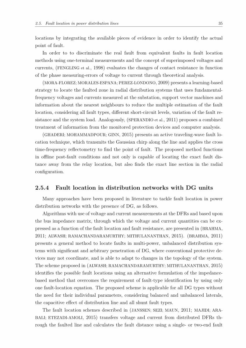
2.5.4 Fault location in distribution networks with DG units
Many approaches have been proposed in literature to tackle fault location in powerdistribution networks with the presence of DG, as follows.
Algorithms with use of voltage and current measurements at the DFRs and based uponthe bus impedance matrix, through which the voltage and current quantities can be ex-pressed as a function of the fault location and fault resistance, are presented in (BRAHMA,2011; ALWASH; RAMACHANDARAMURTHY; MITHULANANTHAN, 2015). (BRAHMA, 2011)presents a general method to locate faults in multi-power, unbalanced distribution sys-tems with significant and arbitrary penetration of DG, where conventional protective de-vices may not coordinate, and is able to adapt to changes in the topology of the system.The scheme proposed in (ALWASH; RAMACHANDARAMURTHY; MITHULANANTHAN, 2015)identifies the possible fault locations using an alternative formulation of the impedance-based method that overcomes the requirement of fault-type identification by using onlyone fault-location equation. The proposed scheme is applicable for all DG types withoutthe need for their individual parameters, considering balanced and unbalanced laterals,the capacitive effect of distribution line and all shunt fault types.
The fault location schemes described in (JANSSEN; SEZI; MAUN, 2011; MAJIDI; ARA-
BALI; ETEZADI-AMOLI, 2015) transfers voltage and current from distributed DFRs th-rough the faulted line and calculates the fault distance using a single- or two-end fault

location method. Statistical errors on phasors and networks parameters are consideredto obtain an optimal estimation of the fault location in (JANSSEN; SEZI; MAUN, 2011),while (MAJIDI; ARABALI; ETEZADI-AMOLI, 2015) simulates a 13.8 [𝑘𝑉 ] power distributionnetwork with and without measurement noises and presents a satisfactorily performancefor various faults with different resistances.
Extended formulations for general use in distribution systems have been proposed(SALIM et al., 2009; NUNES; BRETAS, 2010), based on calculation of the apparent impedanceand fundamental quantities, considering particularities of the distribution systems, such asload-profile variation with local measurements and the presence of distributed generation.
In turn, (GUO-FANG; YU-PING, 2008) proposes an algorithm for urban distributionsystems with DGs that relies on information about the differential current ratio, which isused to describe the features of the faulted line segment.
An algorithm based on fault currents that uses fault passage indicators and searchesthe tree structure of the distribution network with DG to determine the fault channel andidentify the point of fault is presented in (WU, 2010). In addition, (CONTRERAS; RAMOS,2014) explores the design of a versatile and adaptative fault location algorithm for distri-bution systems with DG that relies on the shortest path optimization problem, applyingDijkstra’s Algorithm, to identify nodes with high correlation with faults. Alternatively,(ZHIHAI et al., 2014) proposes a fault location method that uses the signals provided byfault indicators combined with the distribution power grid state at the fault occurrencetime and a unified network topology model suitable for different power distribution lineswith easy adaptability.
The optimal placement of Phasor Measurement Unit (PMU)s is investigated in (RA-
JEEV; ANGEL; KHAN, 2015), whereas the optimum number and location of automaticsectionalizing switching devices is analysed in (CELLI; PILO, 1999). Both procedures arevalid for both radial and meshed distribution systems. In addition, (HE et al., 2014) pre-sents a fault location method that uses current/voltage sensors sparsely installed in thenetwork and depends on the available sensor locations relative to the fault and the lateralconditions to search all possible paths and calculate the fault distance and fault resistanceby reducing the circuit to an equivalent.
Alternatively, (THUKARAM; KHINCHA; VIJAYNARASIMHA, 2005) presents an artificialneural network and support vector machine approach for fault location in radial dis-tribution systems, using measurements available at the substation, circuit breaker andrelay statuses. The faults are classified according to the reactances of their path using acombination of support vector classifiers and feedforward neural networks.
* * *

37
Chapter 3Review of modelling distributed
generation and load technologies
The modelling of DG and load technologies are reviewed in this chapter, which intro-duces the power conditioning units used together with distinct technologies (Section 3.1)and presents the fault behaviour of wind turbines (Section 3.2), photovoltaic cells (Sec-tion 3.3), fuel cells (Section 3.4), gas micro-turbines (Section 3.5) and loads (Section 3.6).The analytical models studied in this chapter are not applied to the problem of fault loca-tion in this work, since they do not interfere with the proposed fault location algorithms.Nonetheless, the impact of errors in the modelling of DG and load technologies on theaccuracy of the fault location algorithms is discussed later in Chapter 5.
3.1 Power Conditioning Units
This section presents the models applied for the AC-DC rectifiers, DC-DC convertersand DC-AC inverters required to connect some of the DG and load technologies to thegrid. Detailed models for power converters together with the control signals reduce consi-derably the simulation speed; alternatively, average models are preferred to maintain thedesirable accuracy. This work takes the advantages of average models on board duringthe validation studies.
3.1.1 AC-DC rectifiers
AC-DC rectifiers may be uncontrollable or controllable devices (WANG, 2006). Theformer is usually referred to diode bridge rectifiers. A diagram of a three-phase full-bridgerectifier is shown in Figure 3 If 𝐿𝑠 is so small that can be neglected, the average value ofthe output DC voltage ��𝑑𝑐 can be calculated as:
𝑉𝑑𝑐 = 3𝜋
·√
2 · ��𝐿−𝐿 (1)

38 Chapter 3. Review of modelling distributed generation and load technologies
+
_c
bn
LsaIaLs
LsCdc Vdc Zload
Idc
Figure 3 – Three-phase full diode bridge rectifier
Source: (WANG, 2006, p. 194) (adapted)
Idc
+
_c
bn
LsY
Y
Ya
Cdc Vdc Zload
Figure 4 – Three-phase 12-diode bridge rectifier with transformers
Source: (WANG, 2006, p. 195) (adapted)
Where ��𝐿−𝐿 is the AC line-to-line Root Mean Square (RMS) voltage.Alternatively, a Y-Y and a Y-Δ connection transformer may be applied to form a 12-
diode bridge rectifier (WANG, 2006), as illustrated in Figure 4. The phase shift betweenthe two transformer outputs reduces the transition period from 60 degrees to 30 degreesin a period, so the average value of the output DC voltage is obtained through:
𝑉𝑑𝑐 = 6𝜋
·√
2 · ��𝐿−𝐿 (2)
In turn, controllable devices can be firing angle controlled thyristor rectifiers or PulseWidth Modulation (PWM) rectifiers. The former replaces the diodes with thyristors, sothat the output DC voltage can be regulated by controlling the firing angles of thyristors.The firing angle 𝛼 is the angular delay between the time when a thyristor is forwardbiased and the time when a positive current pulse is applied to its gate. For instance, theoutput DC voltage of a six-pulse thyristor rectifier can be calculated according to:
𝑉𝑑𝑐 = 3𝜋
·√
2 · ��𝐿−𝐿 · cos(𝛼) (3)

3.1. Power Conditioning Units 39
3.1.2 DC-DC converters
DC-DC converters are combined to DG units in order to change the output voltageof the generator, when required. Among them, the boost converters and buck convertersare typically applied (WANG, 2006). The average value of the output voltage is given by(4) for a boost converter and (5) for a buck converter.
��𝑑𝑑,𝑜𝑢𝑡 = ��𝑑𝑑,𝑖𝑛1 − 𝑑
(4)
��𝑑𝑑,𝑜𝑢𝑡 = 𝑑 · ��𝑑𝑑,𝑖𝑛 (5)
Where d is the duty ratio of the switching pulse, 0 ≤ 𝑑 < 1.
3.1.3 DC-AC inverters
A three-phase six-switch DC-AC PWM voltage source inverter is used to convert thepower from DC to AC, connected to the grid through LC filters and coupling inductors.The inverter switching functions are given by (6), where 𝑖 = 1, 2, 3 and 𝑘 = 𝑎, 𝑏, 𝑐, whilethe output phase-to-neutral voltages are calculated through (7):
𝑑*𝑖 =
⎧⎨⎩ 1, 𝑆+𝑘 𝑂𝑁
−1, 𝑆−𝑘 𝑂𝐹𝐹
(6)
⎧⎪⎪⎪⎨⎪⎪⎪⎩𝑣𝑎𝑛 = 𝑑*
12 · ��𝑑𝑐
𝑣𝑏𝑛 = 𝑑*22 · ��𝑑𝑐
𝑣𝑐𝑛 = 𝑑*32 · ��𝑑𝑐
(7)
The phase-to-phase output voltages can be found by adding the neutral voltage 𝑣𝑛𝑛′
to (7):⎧⎪⎪⎪⎨⎪⎪⎪⎩𝑣𝑎𝑛′ = 𝑣𝑎𝑛 + 𝑣𝑛𝑛′
𝑣𝑏𝑛′ = 𝑣𝑏𝑛 + 𝑣𝑛𝑛′
𝑣𝑐𝑛′ = 𝑣𝑐𝑛 + 𝑣𝑛𝑛′
(8)
3.1.4 Impact of power-converter-interfaced DGs on short-circuitlevels
Typical short-circuit levels of power converters connected to the terminals of DG unitsare presented in table 3, in agreement with the findings from (BARKER; MELLO, 2000).For inverters, the fault contribution depends on the maximum current level and durationfor which the current limiter is set to respond; fault contribution may last for less thanone cycle in some cases and much longer in other cases. For synchronous generators, thefault contribution depends on the pre-fault voltage, sub-transient and transient reactances

40 Chapter 3. Review of modelling distributed generation and load technologies
Table 3 – Typical fault levels of power-converter-interfaced DGs
Generator type Fault current into short-circuited terminals as a percentage ofthe rated output current
Inverter-connected 100-400% (duration depends on controller settings and cur-rent may be less than 100% for some inverters)
Separately excited SG 500-1000% for the first few cycles and decaying to 200-400%
IG or self-excited SG 500-1000% for the first few cycles and decaying to a negligibleamount within 10 cycles
of the machine and excitation characteristics. For induction generators, the fault contri-bution lasts as long as they remain excited by residual voltages on the feeder; for mostof them, significant currents only last a few cycles and may be determined by dividingthe pre-fault voltage by the transient reactance of the machine; in spite of the short timeinterval, it is long enough to impact fuse-breaker coordination in some cases.
3.2 Fault Behaviour of Wind Turbines
3.2.1 Wind turbine concepts
Wind turbines can be distinguished in accordance with their operation and controlprinciples (AKHMATOV, 2003; LINDGREN; SVENSSON; GERTMAR, 2012), as follows:– fixed-speed or variable-speed wind turbines;
– fixed-pitch or variable-pitch wind turbines;
– connected to AC grids directly or through partial- or full-scale power converters.In spite of the differences above, common features characterize the existing concepts
and their interaction with the power grid, which allows the systematization needed toproduce generic but sufficiently realistic models of the wind turbines. Based on thesesimilarities, four Wind Turbine Generator (WTG) technologies have been defined (AKH-
MATOV, 2003; LINDGREN; SVENSSON; GERTMAR, 2012; FOX, 2007; VITTAL; AYYANAR,2012; SULLA, 2012):– type 1 : fixed-speed wind turbines with Squirrel-Cage Induction Generator (SCIG) (with
or without blade-angle control);
– type 2 : wind turbines equipped with Wound Rotor Induction Generator (WRIG) andlimited speed variation through an external variable resistor;
– type 3 : variable-speed, pitch-controlled wind turbines equipped with Doubly-Fed In-duction Generator (DFIG) (connected to the grid at the stator terminals and at therotor windings via partial-scale power converter);
3.2. Fault Behaviour of Wind Turbines 41
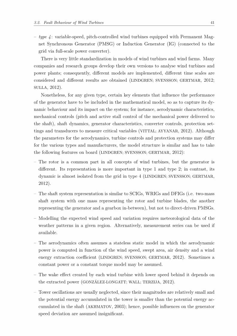
– type 4 : variable-speed, pitch-controlled wind turbines equipped with Permanent Mag-net Synchronous Generator (PMSG) or Induction Generator (IG) (connected to thegrid via full-scale power converter).There is very little standardization in models of wind turbines and wind farms. Many
companies and research groups develop their own versions to analyse wind turbines andpower plants; consequently, different models are implemented, different time scales areconsidered and different results are obtained (LINDGREN; SVENSSON; GERTMAR, 2012;SULLA, 2012).
Nonetheless, for any given type, certain key elements that influence the performanceof the generator have to be included in the mathematical model, so as to capture its dy-namic behaviour and its impact on the system; for instance, aerodynamic characteristics,mechanical controls (pitch and active stall control of the mechanical power delivered tothe shaft), shaft dynamics, generator characteristics, converter controls, protection set-tings and transducers to measure critical variables (VITTAL; AYYANAR, 2012). Althoughthe parameters for the aerodynamics, turbine controls and protection systems may differfor the various types and manufacturers, the model structure is similar and has to takethe following features on board (LINDGREN; SVENSSON; GERTMAR, 2012):
– The rotor is a common part in all concepts of wind turbines, but the generator isdifferent. Its representation is more important in type 1 and type 2; in contrast, itsdynamic is almost isolated from the grid in type 4 (LINDGREN; SVENSSON; GERTMAR,2012).
– The shaft system representation is similar to SCIGs, WRIGs and DFIGs (i.e. two-massshaft system with one mass representing the rotor and turbine blades, the anotherrepresenting the generator and a gearbox in-between), but not to direct-driven PMSGs.
– Modelling the expected wind speed and variation requires meteorological data of theweather patterns in a given region. Alternatively, measurement series can be used ifavailable.
– The aerodynamics often assumes a stateless static model in which the aerodynamicpower is computed in function of the wind speed, swept area, air density and a windenergy extraction coefficient (LINDGREN; SVENSSON; GERTMAR, 2012). Sometimes aconstant power or a constant torque model may be assumed.
– The wake effect created by each wind turbine with lower speed behind it depends onthe extracted power (GONZÁLEZ-LONGATT; WALL; TERZIJA, 2012).
– Tower oscillations are usually neglected, since their magnitudes are relatively small andthe potential energy accumulated in the tower is smaller than the potential energy ac-cumulated in the shaft (AKHMATOV, 2003); hence, possible influences on the generatorspeed deviation are assumed insignificant.

42 Chapter 3. Review of modelling distributed generation and load technologies
Inductiongenerator
TurbinetransformerPower factor
correctioncapacitor
Anti-parallelthyristor
soft-starter
Horizontalaxis in rotor
Gearbox
Pendantcable in tower
To thenetwork
Figure 5 – Schematic of a fixed-speed wind turbine
Source: (FOX, 2007, p. 71) (adapted)
Different wind turbine concepts deliver different fault currents into the grid duringshort-circuits (SULLA, 2012; LINDGREN; SVENSSON; GERTMAR, 2012; VITTAL; AYYANAR,2012). The next topics describe the characteristics of each concept mentioned above,focusing on the fault behaviour.
3.2.1.1 Type 1
Fixed-speed wind turbines comprise an aerodynamic rotor that drives a low-speedshaft, a gearbox, a high-speed shaft and an induction generator. The induction genera-tor is directly connected to the grid and transmits power to a switchboard and a localtransformer (FOX, 2007), as illustrated in Figure 5.
The fixed speed is determined by the gearbox and the number of pole pairs of theinduction generator. Switched capacitors are used to improve the power factor and ananti-parallel thyristor soft-starter is used to build up the magnetic flux and minimizecurrent transients when the generator is powered up. A pitch-regulated rotor controlsthe generator speed during the starting period, but the fixed-pitch, stall-regulated windturbine runs driven by the wind. Due to the steep torque versus slip characteristic of theinduction generator, it operates at about constant speed set by the grid frequency with aslip around 2% at rated power (AKHMATOV, 2003).
A torque pulsation is developed at the blade passing frequency due to the rotor ae-rodynamics, tower shadow and wind shear effects. As such oscillations are usually close tothe natural frequency of the synchronous generator, nowadays the fixed-speed wind tur-bines are equipped with induction machines; some early wind turbines with synchronous

3.2. Fault Behaviour of Wind Turbines 43
generators include mechanical dampers in the drive train, though.
The theoretical behaviour of the induction machine is well-known in literature (KUN-
DUR; BALU; LAUBY, 1994; SULLA, 2012). The induction machine consists of the stator androtor windings. When balanced three-phase currents flow through the stator winding, amagnetic field rotating at synchronous speed 𝑛𝑠 is produced and the relative movementbetween stator and rotor fields induces voltages at the slip frequency 𝑓𝑟 in the rotor win-dings. The electromotive force (EMF) magnitude is proportional to the slip. If the rotoris stationary, then it can be regarded as a transformer. The rotor voltage is proportio-nal to the slip, while the rotor phase current for a given slip is determined by the rotorphase voltage applied across the rotor impedance, which consists of a resistance 𝑅𝑟 andan inductance 𝐿𝑟:
𝐼𝑟 = 𝑠·��𝑟
𝑅𝑟+𝑗·𝑠·𝑋𝑟(9)
The grid determines the voltage when the wind turbine generator and capacitor areconnected to the power network. If a fault occurs, the turbine accelerates and draws alarge amount of reactive power from the grid. The unbalance between mechanical andelectric power may lead the generator to accelerate beyond the critical speed and becomeunstable. Such behaviour may request disconnection and use of an emergency brake andposes a challenge to voltage recovery, as the amount of reactive power drawn after thefault clearance may result in prolonged voltage sags in the grid (SULLA, 2012). Therefore,generator over-speeding and voltage recovery are the main issues for Grid-Fault Ride-Through (GFRT) of fixed-speed wind turbines. This can be prevented by limiting thecapacitor bank sizes and/or adjusting the protection to trip them quickly.
Short-circuits in the grid are usually detected by monitoring fault currents from largesynchronous generators. Induction generators cannot be considered a reliable source offault currents because the time interval (only during the sub-transient period under three-phase short-circuits) is too short for reliable operation of the over-current relays. Thus,it is a common practice to rely on the short-circuit currents from the network in order tooperate protection to isolate the wind farm and trip the wind turbines (FOX, 2007); then,the wind turbine is an open circuit. Nonetheless, the magnitude of the machine currentis crucial to evaluate the response of the wind turbine protection system.
The usual description of the induction machine is the fifth-order model, whose equa-tions in the per unit (p.u.) system can be written as follows (KUNDUR; BALU; LAUBY,1994; AKHMATOV, 2003; PETRU; THIRINGER, 2002; MARTINS et al., 2007; MORREN; HAAN,

44 Chapter 3. Review of modelling distributed generation and load technologies
2007):
⎧⎪⎪⎪⎪⎪⎪⎪⎪⎪⎪⎪⎪⎪⎪⎪⎪⎪⎪⎪⎪⎪⎨⎪⎪⎪⎪⎪⎪⎪⎪⎪⎪⎪⎪⎪⎪⎪⎪⎪⎪⎪⎪⎪⎩
��𝑑𝑠 = 𝐿𝑠 · 𝐼𝑑𝑠 + 𝐿𝑚 · 𝐼𝑑𝑟��𝑞𝑠 = 𝐿𝑠 · 𝐼𝑞𝑠 + 𝐿𝑚 · 𝐼𝑞𝑟��𝑑𝑠 = 𝑅𝑠 · 𝐼𝑑𝑠 − 𝜔𝑠 · ��𝑞𝑠 + 𝑑��𝑑𝑠
𝑑𝑡
��𝑞𝑠 = 𝑅𝑠 · 𝐼𝑞𝑠 + 𝜔𝑠 · ��𝑑𝑠 + 𝑑��𝑞𝑠
𝑑𝑡
��𝑑𝑟 = 𝐿𝑟 · 𝐼𝑑𝑟 + 𝐿𝑚 · 𝐼𝑑𝑠��𝑞𝑟 = 𝐿𝑟 · 𝐼𝑞𝑟 + 𝐿𝑚 · 𝐼𝑞𝑠��𝑑𝑟 = 𝑅𝑟 · 𝐼𝑑𝑟 − 𝑠 · 𝜔𝑠 · ��𝑞𝑟 + 𝑑��𝑑𝑟
𝑑𝑡
��𝑞𝑟 = 𝑅𝑟 · 𝐼𝑞𝑟 + 𝑠 · 𝜔𝑠 · ��𝑑𝑟 + 𝑑��𝑞𝑟
𝑑𝑡
𝑇𝐸 = ��𝑑𝑠 · 𝐼𝑞𝑠 − ��𝑞𝑠 · 𝐼𝑑𝑠
(10)
Where 𝑅𝑠, 𝐿𝑠, 𝑅𝑟, 𝐿𝑟 and 𝐿𝑚 are the stator resistance and inductance, rotor resistanceand inductance and mutual inductance, respectively. ��𝑠 = (𝑉𝑑𝑠, 𝑉𝑞𝑠) is the terminalvoltage, 𝐼𝑠 = (𝐼𝑑𝑠, 𝐼𝑞𝑠) is the stator current, 𝜓𝑠 = (𝜓𝑑𝑠, 𝜓𝑞𝑠) is the stator flux. The rotorvoltage ��𝑟 = (𝑉𝑑𝑟, 𝑉𝑞𝑟) is zero because the rotor circuit is shorted. 𝐼𝑟 = (𝐼𝑑𝑟, 𝐼𝑞𝑟) is therotor current, 𝜓𝑟 = (𝜓𝑑𝑟, 𝜓𝑞𝑟) is the rotor flux in the stator quantities, whilst 𝑇𝐸 is theelectrical torque. This is the fifth-order model with addition of the movement equationof the generator rotor and representation of the fundamental-frequency transients of thestator current, given by the derivatives of the stator flux.
The currents can be written in function of the fluxes, as in (11):
⎧⎪⎪⎨⎪⎪⎩𝐼𝑠 = 1
𝐿𝑠− 𝐿2𝑚
𝐿𝑟
· ��𝑠 − 𝐿𝑚
𝐿𝑟· 1𝐿𝑠− 𝐿2
𝑚𝐿𝑟
· ��𝑟
𝐼𝑟 = −𝐿𝑚
𝐿𝑠· 1𝐿𝑟− 𝐿2
𝑚𝐿𝑠
· ��𝑠 + 1𝐿𝑟− 𝐿2
𝑚𝐿𝑠
· ��𝑟(11)
Alternatively, the short-circuit current can be calculated through the superpositionmethod, as in (SULLA, 2012), comprising a component for the post-fault steady statevoltage at the generator terminals and for the natural stator and rotor fluxes. The naturalstator and rotor fluxes arise after the fault occurrence to assure the flux continuity beforeand after the fault inception, then decay exponentially with time constants that dependon the generator parameters. Once known the post-fault transient fluxes, the short-circuitcurrent can be calculated, comprising an AC and a DC component that decay respectivelywith the rotor and the stator transient time constants and are limited by the transientreactance, usually varying between 5 and 9 times the generator rated current (SULLA,2012).
The third-order model is derived from the fifth-order one (10) by omitting the fundamental-frequency transients in the stator:
𝑑𝜓𝑠
𝑑𝑡=
(𝑑𝜓𝑑𝑠
𝑑𝑡, 𝑑𝜓𝑞𝑠
𝑑𝑡
)= (0, 0) (12)

3.2. Fault Behaviour of Wind Turbines 45
+ . .R + jX'SS
v + jv'qsds
i + ji'qsds
. .v + jv'qd
Figure 6 – Induction generator third-order model neglecting stator transients
Source: (MARTINS et al., 2007, p. 2) (adapted)
.v g
.v s
i g i s i r
L r
L mC
L sL gR g R s
R /s s
Figure 7 – Equivalent circuit of the induction generator ninth-order model, reactive power compensatingcapacitor and grid
Source: (PETRU; THIRINGER, 2002, p. 4) (adapted)
It results in a simplified model of the induction machine connected to the grid as avoltage source �� ′
𝑑 + 𝑗 · �� ′𝑞 (referred to the stator) behind a transient impedance 𝑋𝑑+ 𝑗 ·𝑋𝑞
(MARTINS et al., 2007), according to (13) and Figure 6.
⎧⎪⎪⎪⎨⎪⎪⎪⎩𝑑�� ′
𝑑
𝑑𝑡= − 1
𝜏·
[�� ′𝑑 − (𝑋𝑠 −𝑋 ′
𝑠) · 𝐼𝑞𝑠]
+ 𝑗 · 𝑠 · 𝜔𝑠 · �� ′𝑞
𝑑�� ′𝑞
𝑑𝑡= − 1
𝜏·
[�� ′𝑞 − (𝑋𝑠 −𝑋 ′
𝑠) · 𝐼𝑑𝑠]
+ 𝑗 · 𝑠 · 𝜔𝑠 · �� ′𝑑
𝑇𝐸 = �� ′𝑑 · 𝐼𝑑𝑠 + �� ′
𝑞 · 𝐼𝑞𝑠
(13)
Where 𝜏 = 𝑋𝑟
𝑅𝑟and 𝑋 ′
𝑠 = 𝑋𝑠 − 𝑋2𝑚
𝑋𝑟. Likewise to the third-order model, the first-order
one can be obtained by neglecting the transients in the rotor flux 𝜓𝑟.When the reactive power compensation capacitor is involved in the study, the supply
grid also have to be included; as a consequence, the model complexity is increased to theninth order. The equations in the p.u. system can be written as (14) (PETRU; THIRINGER,2002) and the equivalent circuit is illustrated in Figure 7:
⎧⎪⎪⎪⎪⎪⎪⎪⎪⎪⎨⎪⎪⎪⎪⎪⎪⎪⎪⎪⎩
��𝑔 = (𝑅𝑔 + 𝑗 · 𝜔𝑠 · 𝐿𝑔) · 𝐼𝑔 + 𝐿𝑔 · 𝑑𝐼𝑔
𝑑𝑡+ ��𝑠
��𝑠 = (𝑅𝑠 + 𝑗 · 𝜔𝑠 · 𝐿𝑠) · 𝐼𝑠 + +𝑗 · 𝜔𝑠 · 𝐿𝑚 · 𝐼𝑟 + 𝐿𝑠 · 𝑑𝐼𝑠
𝑑𝑡+ 𝐿𝑟 · 𝑑𝐼𝑟
𝑑𝑡
0 = (𝑅𝑟 + 𝑗 · 𝜔𝑟 · 𝐿𝑟) · 𝐼𝑟 + 𝑗 · 𝜔𝑟 · 𝐿𝑚 · 𝐼𝑠 + 𝐿𝑚 · 𝑑𝐼𝑠
𝑑𝑡+ 𝐿𝑟 · 𝑑𝐼𝑟
𝑑𝑡
𝐼𝑠 − 𝐼𝑟 = 𝑗 · 𝜔𝑠 · 𝐶 · ��𝑠 + 𝐶 · 𝑑��𝑠
𝑑𝑡
𝑇𝐸 = 𝑝 · 𝐿𝑚 · 𝐼𝑚𝑎𝑔{𝐼𝑠 · 𝐼𝑟*
}(14)
Models of lower order than the fifth are usually applied to power system studies, butthey may lead to inaccuracies (MARTINS et al., 2007; PETRU; THIRINGER, 2002). Forinstance, it is shown in (PETRU; THIRINGER, 2002) that the response to shaft torquedisturbances is similar above the third order. However, the braking torque versus rotor
46 Chapter 3. Review of modelling distributed generation and load technologies
speed curve of the induction generator are discrepant: when the fundamental-frequencytransients in the stator are neglected in third-order models, their speed increases immedi-ately after the fault occurrence, whereas it decreases in fifth-order models in such a waythat a notch is produced in the speed curve (AKHMATOV, 2003). Moreover, the responseto voltage dips reveals more differences between the models: the first-order model doesnot provide any acceptable results; the fifth and ninth-order ones predict surge currentsduring the first line periods and the latter also predicts a high-frequency oscillation dueto the capacitor (PETRU; THIRINGER, 2002). To achieve high accuracy, the evaluation ofmajor grid disturbances requests the representation of the skin effect and saturation of le-akage inductances; therefore, models of at least the fifth order are recommended (PETRU;
THIRINGER, 2002).The short-circuit behaviour of fixed-speed wind turbines is determined by the dynamics
of the generator (SULLA, 2012; PETRU; THIRINGER, 2002; AKHMATOV, 2003; THIRINGER;
PETERSSON; PETRU, 2003). High short-circuit currents are delivered during the fault,decaying with the fluxes in the generator stator and rotor. A method for calculating theshort-circuit current of a SCIG is presented in (KANELLOS; KABOURIS, 2009; MORREN;
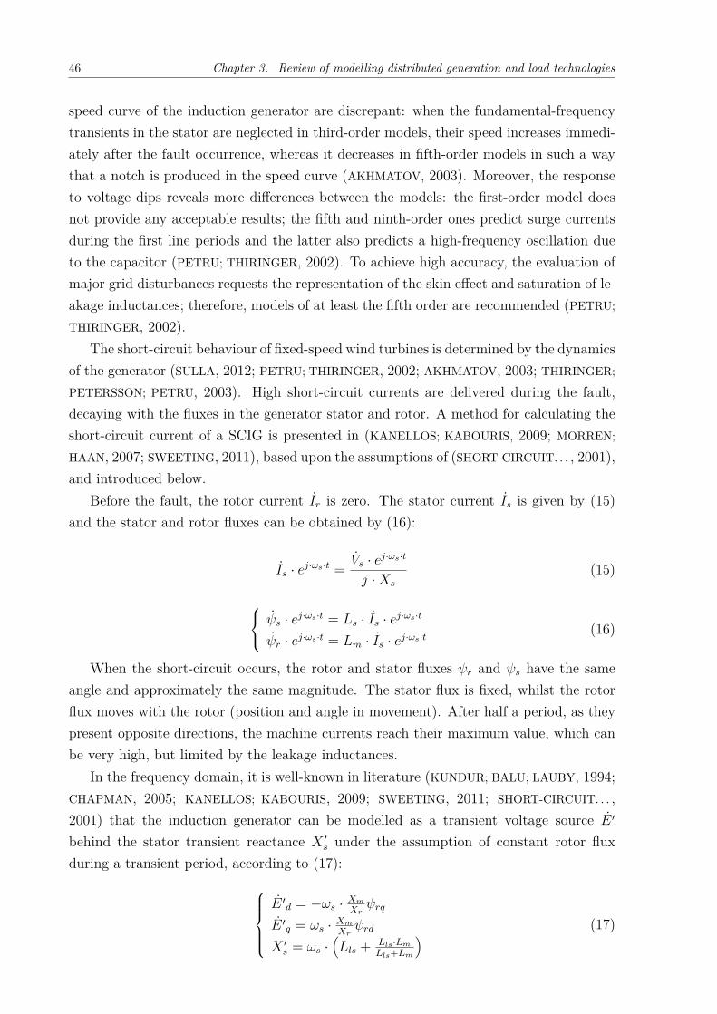
HAAN, 2007; SWEETING, 2011), based upon the assumptions of (SHORT-CIRCUIT. . . , 2001),and introduced below.
Before the fault, the rotor current 𝐼𝑟 is zero. The stator current 𝐼𝑠 is given by (15)and the stator and rotor fluxes can be obtained by (16):
𝐼𝑠 · 𝑒𝑗·𝜔𝑠·𝑡 = ��𝑠 · 𝑒𝑗·𝜔𝑠·𝑡
𝑗 ·𝑋𝑠
(15)
⎧⎨⎩ ��𝑠 · 𝑒𝑗·𝜔𝑠·𝑡 = 𝐿𝑠 · 𝐼𝑠 · 𝑒𝑗·𝜔𝑠·𝑡
��𝑟 · 𝑒𝑗·𝜔𝑠·𝑡 = 𝐿𝑚 · 𝐼𝑠 · 𝑒𝑗·𝜔𝑠·𝑡 (16)
When the short-circuit occurs, the rotor and stator fluxes 𝜓𝑟 and 𝜓𝑠 have the sameangle and approximately the same magnitude. The stator flux is fixed, whilst the rotorflux moves with the rotor (position and angle in movement). After half a period, as theypresent opposite directions, the machine currents reach their maximum value, which canbe very high, but limited by the leakage inductances.
In the frequency domain, it is well-known in literature (KUNDUR; BALU; LAUBY, 1994;CHAPMAN, 2005; KANELLOS; KABOURIS, 2009; SWEETING, 2011; SHORT-CIRCUIT. . . ,2001) that the induction generator can be modelled as a transient voltage source �� ′
behind the stator transient reactance 𝑋 ′𝑠 under the assumption of constant rotor flux
during a transient period, according to (17):⎧⎪⎪⎪⎨⎪⎪⎪⎩�� ′
𝑑 = −𝜔𝑠 · 𝑋𝑚
𝑋𝑟𝜓𝑟𝑞
�� ′𝑞 = 𝜔𝑠 · 𝑋𝑚
𝑋𝑟𝜓𝑟𝑑
𝑋 ′𝑠 = 𝜔𝑠 ·
(𝐿𝑙𝑠 + 𝐿𝑙𝑠·𝐿𝑚
𝐿𝑙𝑠+𝐿𝑚
) (17)

3.2. Fault Behaviour of Wind Turbines 47
The stator short-circuit current can be obtained by substituting (16) at 𝑡 = 0 (refe-rence) in 𝐼𝑠 from (11). Then, the stator short-circuit current can be obtained accordingto (18):
𝐼𝑠 =√
2 · ��𝑠𝑗 ·𝑋 ′
𝑠
·[𝑒
−𝑡𝑇 ′
𝑠 − (1 − 𝜎) · 𝑒𝑗·𝜔𝑠·𝑡 · 𝑒−𝑡𝑇 ′
𝑟
](18)
Where⎧⎪⎪⎪⎪⎪⎪⎪⎪⎪⎨⎪⎪⎪⎪⎪⎪⎪⎪⎪⎩
𝜎 = 1 − 𝐿2𝑚
(𝐿𝑙𝑠+𝐿𝑚)(𝐿𝑙𝑟+𝐿𝑚)
𝑇 ′𝑠 = 𝐿′
𝑠
𝑅𝑠
𝑇 ′𝑟 = 𝐿′
𝑟
𝑅𝑟
𝐿′𝑠 = 𝐿𝑙𝑠 + 𝐿𝑙𝑟·𝐿𝑚
𝐿𝑙𝑟+𝐿𝑚
𝐿′𝑟 = 𝐿𝑙𝑟 + 𝐿𝑙𝑠·𝐿𝑚
𝐿𝑙𝑠+𝐿𝑚
(19)
The parameters 𝐿𝑚, 𝐿𝑙𝑠 and 𝐿𝑙𝑟 denote the mutual, stator and rotor leakage induc-tances, respectively. The stator short-circuit current comprises a DC component dampedwith the stator transient time constant 𝑇 ′
𝑠 and an AC component damped with the rotortransient time constant 𝑇 ′
𝑟. Although the current vector does not reach the maximumvalue exactly at 𝑡 = 𝑇
2 , the value after half a period provides a good approximation ofthe maximum current (KANELLOS; KABOURIS, 2009; MORREN; HAAN, 2007), which canbe obtained by substituting 𝑡 = 𝑇
2 in (18). If the analysis aims to calculate the maxi-mum RMS value of the AC current component, then the stator voltage before the faultoccurrence and the stator transient reactance shall be used (KANELLOS; KABOURIS, 2009).
When the voltage ��𝑠 has a phase displacement of 𝛼 + 𝜋2 with respect to the stator at
the instant of occurrence of the fault, it shall be replaced with 𝑗 ·√
2 · ��𝑠 · 𝑒𝑗·𝛼. Then,the short-circuit current in a phase is given by the projection of the vector 𝐼𝑠 (MORREN;
HAAN, 2007):
𝐼𝑠 =√
2·��𝑠
𝑋′𝑠
·[𝑒
− 𝑡𝑇 ′
𝑠 · cos (𝛼) − (1 − 𝜎) · 𝑒𝑗·𝜔𝑠·𝑡 · 𝑒− 𝑡𝑇 ′
𝑟 · cos (𝜔𝑠 · 𝑡+ 𝛼)]
(20)
3.2.1.2 Type 2
These wind turbines are equipped with doubly-outage induction generators and avariable external resistance connected in series with the rotor winding and controlled bythe rotor converter, so as to achieve a limited range of speed variation. A schematic isshown in Figure 8. The rotor resistance, mounted on the stator shaft, can be controlledwith optical signals (AKHMATOV, 2003; SULLA, 2012; THIRINGER; PETERSSON; PETRU,2003) to avoid the request for slip rings. The external resistor is pulsed through a DCchopper circuit with variable duty cycle, which results in a variable resistance withoutmoving parts. This arrangement produces a limited variation in the generator speed(around 10%) and a constant power output, albeit the changes in the wind speed, andoperation at variable slip above the synchronous speed (AKHMATOV, 2003).

48 Chapter 3. Review of modelling distributed generation and load technologies
Inductiongenerator
Variableresistance
TurbinetransformerPower factor
correctioncapacitor
Anti-parallelthyristor
soft-starter
Horizontalaxis in rotor
Gearbox
Pendantcable in tower
To thenetwork
Figure 8 – Schematic of a wind turbine with variable external resistance
Source: author
The total value of the dynamic rotor resistance is the sum of the stationary rotorwinding resistance and the dynamic external rotor resistance (SULLA, 2012). In normaloperation, a low value of the rotor resistance minimizes power losses. In turn, when agrid fault occurs, the rotor resistance increases, consequently the maximum torque ofthe torque versus slip characteristic is shifted towards higher slip and higher generatorspeed (SULLA, 2012); when the voltage is re-established, the rotor resistance is reducedagain.
The short-circuit behaviour of a limited-variable speed wind turbine is conditioned bythe dynamics of the generator (SULLA, 2012; MARTINEZ et al., 2011; AKHMATOV, 2003),similarly to the type 1 wind turbines. As a result, the models in the frequency domainare the same for types 1 and 2 wind turbines, except for the external resistance added tothe rotor resistance in the latter, which causes a rapid decay of the AC component of thestator current (SULLA, 2012; MARTINEZ et al., 2011).
An important constraint of fixed-speed WTGs is that they can over-speed and losestability in case of voltage depression caused by short-circuits. Besides, the low terminalvoltage results in over-speed of the generator and a high drawn of reactive power thatdecreases the grid voltage further and leads to collapse. An external capacitor bankmust be provided for reactive support, since the reactive power consumption cannot becontrolled independently of the active power.

3.2. Fault Behaviour of Wind Turbines 49
To thenetwork
Crowbarprotection
Controller
C1
AC/DC
C2
DC/AC
P + jQgg
.V r
.I r
.I s
.I g
.V s
Figure 9 – Schematic of a DFIG wind turbine
Source: (FOX, 2007, p. 74) (adapted)
3.2.1.3 Type 3
The DFIG comprises a wound rotor induction generator with the stator directly con-nected to the grid and the rotor connected to the grid through slip rings and a back-to-backpartial-load converter, which takes current into or out of the rotor windings. The rotorconverter is controlled by power electronics with Insulated-gate bipolar transistor (IGBT)-switches so as to decouple the network electrical frequency from the desired rotationalspeed. Variable-speed operation is achieved by controlling the rotor voltage at the slipfrequency.
The voltage in the stator is applied from the grid and the voltage in the rotor isinduced by the converter. The rotor-side converter (RSC) is coupled through a capacitorto the grid-side converter (GSC), which is connected to the grid through a transformer.
The DFIG supplies electric power to the grid at super-synchronous speed (from thestator and rotor) with high mechanical input power and absorbs power from the grid atsub-synchronous speed (from the rotor through the converters) with low mechanical inputpower. Therefore, the power flow through the rotor can be bidirectional. At synchronousspeed, the net power exchange between rotor and grid is irrelevant, as the DC-link ca-pacitor voltage is controlled by the grid-side converter. The total power delivered to thegrid 𝑃𝑔 is the sum of the stator power 𝑃𝑠 and the rotor power 𝑃𝑟, as presented in (FOX,2007) and illustrated in Figure 9.
The DFIG is controlled by the converters for frequency/reactive power, voltage/reactive

50 Chapter 3. Review of modelling distributed generation and load technologies
power and pitch angle/mechanical power (VITTAL; AYYANAR, 2012). It is possible to varythe injected power by acting on the back-to-back converter, particularly by controllingthe current through the RSC. Hence, the current-controlled RSC can be seen as a con-trolled current source in parallel to the DFIG magnetization reactance. In addition, if aThevenin equivalent impedance is substituted in parallel to these two elements, the DFIGmodel will match the synchronous generator and the power control will be simple.
A common practice uses the RSC to provide torque and speed control together withvoltage or power factor control for the overall system, and the GSC to maintain the DC-link voltage level and provide a path for the rotor power to flow to and from the AC system.As the reactive power injection through the rotor circuit is inversely proportional to theslip, the RSC is preferred to the GSC on voltage-control schemes. Further explanationsare given in (FOX, 2007).
The power flow simulation provides the operating condition to set up the time-domaintransient stability study of the machine in consideration. The active and reactive poweroutput and the terminal voltage at the WTG bus are used to initialize the model, whereasthe outputs provide the current injected by the generator into the network. The electricalpower output of the WTG is used to calculate the reference rotor speed according to dataprovided by the manufacturer (VITTAL; AYYANAR, 2012; AKHMATOV, 2003).
The DFIG can be excited from the rotor circuit by the converter, not necessarily fromthe power grid (AKHMATOV, 2003). If connected to a strong power system at aroundrated voltage, the generator will be excited by the RSC, produce active power and notexchange reactive power with the grid; in turn, if connected to a weak power systemwith fluctuating voltages, the generator will produce active power and also be requiredto produce or absorb reactive power to control the voltage level at the connection point.
In comparison to conventional asynchronous generators, DFIGs may be advantageousdue to the reactive power and voltage control and the decoupling of active and reactivepower control with independent control of torque and rotor excitation current (AKHMA-
TOV, 2003). It can be achieved by adjusting the external voltage applied to the rotorso as to control the stator current (SULLA, 2012) and by representing the generator in adirect-quadrature (d-q) axis reference frame rotating at synchronous speed (FOX, 2007).Reactive power support to the grid can be provided by the stator by changing the d-axisrotor excitation current, as well as power factor and torque regulation.
The partial-load converter is usually rated to handle the rotor power and the generatorexcitation (magnetization from the rotor circuit). Its power capacity is smaller than thefull-load converter; on the one hand, it reduces the size and cost of the converter, asit is sized to approximately 30% of the rated power and the power flowing through therotor is given by the product of the stator power and the slip (TEODORESCU; LISERRE;
RODRÍGUEZ, 2010); on the other hand, the power electronics are the most sensitive parts ofthis wind turbine concept and transient grid disturbances may lead to converter blocking

3.2. Fault Behaviour of Wind Turbines 51
and disconnection of the wind turbine. Thus, the current flowing through both the RSCand GSC must be limited.
The voltage drop at the WTG terminals during short-circuits results in large oscillatorycurrents in the stator windings that also flow through the rotor circuit and the powerconverter due to the magnetic coupling between stator and rotor. Theoretically, the RSCcould be oversized to handle the short-circuit current, but it would increase the costsand the main advantage of this turbine concept would disappear. Therefore, the powerconverter system shall be equipped with a protective system to monitor the converter,generator and grid operation at the generator terminals and order the converter to blockwhen one of the monitored parameters exceeds the relay settings so as to protect thesystem against electrical and thermal overload (MORREN; HAAN, 2007). Typical blockingtimes can be of a few milliseconds (AKHMATOV, 2003).
The RSC, GSC, DC-link and converter control also have to be represented. Whenonly the RSC is considered, the transients in the rotor current are higher than when theGSC and the DC-link are also added to the model, because the DC-link capacitor storagesenergy and thereby interacts with the RSC, exchanging electrical energy during transientevents and producing voltage fluctuations at the DC-link. It introduces delays betweenthe RSC and GSC and smooths the active and reactive power profiles.
Therefore, the converter action could well decide the operation of this wind turbineconcept during transient events in the grid. As the setting of the overload protectionis not well above the rated current, accurate prediction of fault currents is important toobtain accurate results. Thus, modelling of the generator shall be accurate and detailed torepresent the converter blocking sequences in short-term analyses. The response to smallgrid disturbances is mainly determined by the control algorithms, whereas the responseto large grid disturbances is also dependent of the system configuration. In case of largegrid faults, it may be necessary to short-circuit the rotor in order to protect the converter(THIRINGER; PETERSSON; PETRU, 2003; PETRU; THIRINGER, 2002; AKHMATOV, 2003).The stator disconnection through circuit breakers lasts a few cycles; meanwhile, the DFIGacts as a fixed-speed wind turbine and the induction machine goes from the pre-fault speedvalue to a nearly synchronous one and farther contributes to the fault current due to theactive and reactive power exchange with the grid (THIRINGER; PETERSSON; PETRU, 2003).
For protecting the DFIG wind turbine, the rotor circuit may be short-circuited througha crowbar resistance simultaneously to the blocking of the RSC. Alternatively, a DCchopper may be used to maintain the DC-link capacitor voltage within an acceptablerange. For both protection schemes, the current immediately after the fault is determinedby the physical system and not by the control strategy in use; Thus, general conclusionson the delivered short-circuit current may be drawn (SULLA, 2012).
The DFIG contributes to the short-circuit power because the stator is directly connec-ted to the grid; consequently, high currents are produced during grid faults (TEODORESCU;

52 Chapter 3. Review of modelling distributed generation and load technologies
LISERRE; RODRÍGUEZ, 2010; SULLA, 2012; MORREN; HAAN, 2007). The DFIG responsecan be divided in two stages (KANELLOS; KABOURIS, 2009), as follows:– Sub-transient period: during the first 2-3 cycles, the DFIG operates as an SCIG;
– Activation of the protection system: when the crowbar protection system or anothercurrent limitation function of the RSC is activated, the transients of the rotor flux startdecaying and the rotor current is limited.The maximum short-circuit current of a DFIG can be calculated with good accuracy
by using the transient reactance of the induction machine (KANELLOS; KABOURIS, 2009;SULLA, 2012; MORREN; HAAN, 2007). The initial value of the current can be determinedunder the assumption that stator and rotor resistances can be neglected. When the bypassresistor is connected to protect the converter in case of a fault, the current becomes:
𝐼𝑠 · 𝑒𝑗·𝜔𝑠·𝑡 = ��𝑠 · 𝑒𝑗·𝜔𝑠·𝑡
𝑗 ·𝑋𝑠 +𝑅𝑐𝑏
(21)
And the transient time constant of the rotor becomes:
𝑇 ′𝑟 = 𝐿′
𝑟
𝑅𝑟 +𝑅𝑐𝑏
(22)
The assumption that the stator and rotor fluxes are 180 degrees out of phase after half acycle is approximately valid for an induction machine, since the slip is small and the statorand rotor are approximately in phase with each other when the fault occurs. Conversely,a DFIG can operate at much larger slip, typically between -0.3 and +0.3 (TEODORESCU;
LISERRE; RODRÍGUEZ, 2010; SULLA, 2012; AKHMATOV, 2003), which implies that thefluxes are out of phase at the fault occurrence. When the DFIG is in over-synchronousmode, the rotor flux leads the stator one and it takes less than half a period for them tobe 180 degrees out of phase. In turn, when the DFIG is in under-synchronous mode, theopposite happens and it takes more than half a period for the displacement of 180 degrees(KANELLOS; KABOURIS, 2009).
When the voltage at the stator terminals drops to zero, the stator and rotor fluxesrotate slowly, depending on their resistance. It can be neglected for an induction machinebecause of the small resistance, but it is no longer negligible for a DFIG with bypassresistor. This is another reason why the maximum current can be reached in less thanhalf a period. Considering the differences between an induction machine and a DFIG, themaximum current can be written as in (23):
𝐼𝑠 =√
2·��𝑠√𝑋′
𝑠2+𝑅𝑐𝑏
2 ·[𝑒
− Δ𝑡𝑇 ′
𝑠 − (1 − 𝜎) · 𝑒− Δ𝑡𝑇 ′
𝑟
](23)
The time interval Δ𝑡 after which the current reaches its first peak depends on the slipand the value of the bypass resistor.
Alternatively, a general method to calculate the short-circuit current of a DFIG, pre-sented in (SULLA, 2012), deals with both symmetrical and unsymmetrical faults, voltage

3.2. Fault Behaviour of Wind Turbines 53
dips at the WTG terminals and applies a linearised model of the induction machine, ne-glecting saturation of its reactances. As this effect can increase the short-circuit current,the accuracy of the proposed method is affected. Besides, the step-up transformer andMV line impedances also have to be added to the stator impedance, as they are notnegligible.
With crowbar protection, the rotor windings of the DFIG are short-circuited by a setof resistors during a grid fault; then, the current flows through these resistors instead ofthe power converter. Consequently, the fault behaviour of the DFIG depends on whetheror not the crowbar protection is activated.
During the activation period, the DFIG may be assumed as a SCIG with larger rotorresistance (typically up to 20 times the generator resistance) and higher slip, as the controlof the current is lost. The high crowbar resistance leads the AC component of the short-circuit current to decay more rapidly in a DFIG than in a SCIG and after some periodsit is predominantly a DC component. However, when the RSC is reconnected, it controlsthe stator current. Then, the DFIG behaves similarly to a full-load converter inductiongenerator and may be treated as a constant current source. On the top of that, it isimportant to consider that the interval between the fault inception and the insertion ofthe crowbar resistance may adversely affect the accuracy of the proposed method.
The maximum short-circuit current of a DFIG with crowbar protection can be calcu-lated through (23). This result is strongly dependent of the crowbar resistance, whosevalue shall be high enough to limit the short-circuit current and low enough to avoid highvoltage in the rotor circuit (MORREN; HAAN, 2007). However, the crowbar alone may notbe sufficient to achieve GFRT, as the DC-link voltage tends to increase due to the contri-bution of energy from the rotor and a chopper resistance may be required; in this case, thefault behaviour of the DFIG depends on the equivalent resistance formed by the DC-linkcapacitor and chopper resistance connected to the rotor through a diode bridge rectifier.The highest fault current occurs when the RSC is blocked. In turn, unsymmetrical faultsusually produce high rotor voltages due to the negative sequence in the grid that maybe well above the RSC control range. As they do not decay, the crowbar resistance mustremain inserted and the RSC blocked for the whole duration of the fault (SULLA, 2012).
The RSC is blocked after the fault occurrence and the rotor circuit is connected to theDC-link capacitor through the diode bridge formed by the anti-parallel diodes of the RSC.The chopper resistance is switched to maintain the capacitor voltage within acceptablevalues, as the GSC capability is reduced under severe fault conditions. The rotor circuitdemagnetizes and feeds current into the DC-link capacitor; high currents are mainly dueto the natural stator flux that arises to ensure the continuity of flux before and afterthe fault. During the decaying period, the rotor circuit can be regarded as a three-phasedecaying AC voltage source connected through a diode bridge rectifier (anti-parallel diodesof the blocked rotor converter) to a constant DC voltage source supplied by the DC-link
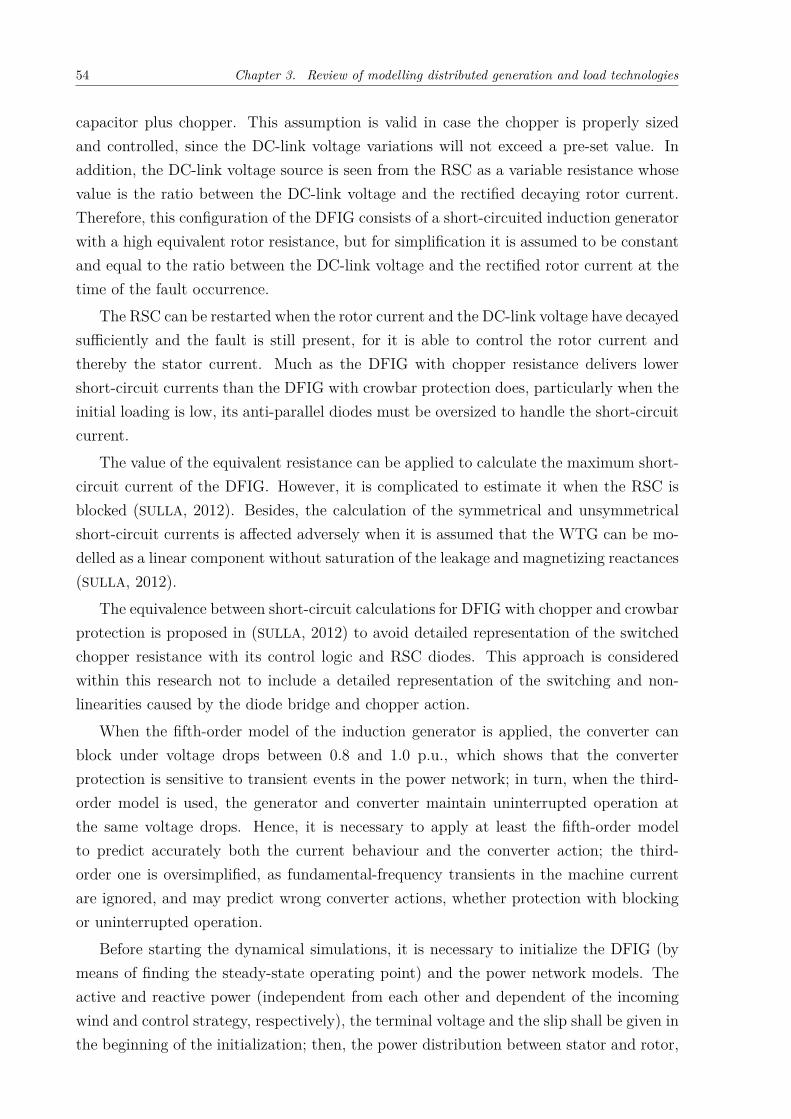
54 Chapter 3. Review of modelling distributed generation and load technologies
capacitor plus chopper. This assumption is valid in case the chopper is properly sizedand controlled, since the DC-link voltage variations will not exceed a pre-set value. Inaddition, the DC-link voltage source is seen from the RSC as a variable resistance whosevalue is the ratio between the DC-link voltage and the rectified decaying rotor current.Therefore, this configuration of the DFIG consists of a short-circuited induction generatorwith a high equivalent rotor resistance, but for simplification it is assumed to be constantand equal to the ratio between the DC-link voltage and the rectified rotor current at thetime of the fault occurrence.
The RSC can be restarted when the rotor current and the DC-link voltage have decayedsufficiently and the fault is still present, for it is able to control the rotor current andthereby the stator current. Much as the DFIG with chopper resistance delivers lowershort-circuit currents than the DFIG with crowbar protection does, particularly when theinitial loading is low, its anti-parallel diodes must be oversized to handle the short-circuitcurrent.
The value of the equivalent resistance can be applied to calculate the maximum short-circuit current of the DFIG. However, it is complicated to estimate it when the RSC isblocked (SULLA, 2012). Besides, the calculation of the symmetrical and unsymmetricalshort-circuit currents is affected adversely when it is assumed that the WTG can be mo-delled as a linear component without saturation of the leakage and magnetizing reactances(SULLA, 2012).
The equivalence between short-circuit calculations for DFIG with chopper and crowbarprotection is proposed in (SULLA, 2012) to avoid detailed representation of the switchedchopper resistance with its control logic and RSC diodes. This approach is consideredwithin this research not to include a detailed representation of the switching and non-linearities caused by the diode bridge and chopper action.
When the fifth-order model of the induction generator is applied, the converter canblock under voltage drops between 0.8 and 1.0 p.u., which shows that the converterprotection is sensitive to transient events in the power network; in turn, when the third-order model is used, the generator and converter maintain uninterrupted operation atthe same voltage drops. Hence, it is necessary to apply at least the fifth-order modelto predict accurately both the current behaviour and the converter action; the third-order one is oversimplified, as fundamental-frequency transients in the machine currentare ignored, and may predict wrong converter actions, whether protection with blockingor uninterrupted operation.
Before starting the dynamical simulations, it is necessary to initialize the DFIG (bymeans of finding the steady-state operating point) and the power network models. Theactive and reactive power (independent from each other and dependent of the incomingwind and control strategy, respectively), the terminal voltage and the slip shall be given inthe beginning of the initialization; then, the power distribution between stator and rotor,

3.2. Fault Behaviour of Wind Turbines 55
the stator and rotor current and the rotor voltage induced by the converter shall be found;after that, the frequency converter shall be initialized with information about the rotorpower neglecting losses. For simplification purposes, fundamental-frequency componentsmay be assumed so as to neglect higher harmonics and losses in the core, windings andconverters, as well as a symmetrical three-phase winding distributed around an uniformair gap.
The stator flux transients are usually neglected for evaluation of dynamic small-signalstability and transient voltage stability, due to the independent power control; consequen-tly, the rotational speed and the terminal voltage are decoupled and the former duringthe fault does not impact the latter after the fault clearance. Neglecting the stator fluxtransients may lead to neglecting the fundamental-frequency transients in the machinecurrents; on the one hand, it does not affect the results under the assumption that theconverter maintains uninterrupted operation and the wind turbine does not disconnectduring the fault; on the other hand, it may be relevant when the short-circuit results ina significant voltage drop and also be influenced by the converter control system.
Operation of variable-speed wind turbines equipped with converter-controlled DFIGsduring grid faults depends mainly on the converter and protective system action. Abnor-mal operating conditions may lead to converter blocking, generator tripping and conse-quently wind turbine disconnection and stopping. Moreover, blocked converters lose theircontrollability and may lead to disconnection of the wind turbine unless a reinitializingroutine is applied.
The idea behind the uninterrupted operation is that the wind turbine does not tripwhen the converter has blocked at a grid fault. The controllability of the RSC is lost whenit is blocked; consequently, the generator behaves as an induction generator without inde-pendent active and reactive power control. After the fault has been cleared and the voltageand frequency have been re-established in the power network, the RSC synchronizes andrestarts on normal operating conditions.
As described in (AKHMATOV, 2003), when the rotor converter blocks, it stops swit-ching and trips; then, the rotor circuit is closed through an external resistor with acurrent-limiting function. In such case, the generator operates as a conventional induc-tion generator with a short-circuited rotor and an increased rotor resistance, whereas thecontrol system of the RSC continues to monitor the electrical parameters, waiting theorder to restart. When the current and the terminal voltage are within the expectedranges, the synchronization starts: the converter starts switching, the external resistanceis switched off and the control system resets the controllers by the measured values. Aftercompleting this procedure, the control system is shifted and the RSC restarts. Theremight be the risk of blocking again because of excessive current transients during thecontrol shifting and incomplete synchronization caused by delays in the measured signalsapplied to reset the controllers.

56 Chapter 3. Review of modelling distributed generation and load technologies
The external resistance is used to reduce the current magnitude when the RSC isblocked. Another request is to damp properly the transients in the rotor circuit beforethe restart. Thus, the external resistance has to be neither too large nor too small, inorder to minimize the risk of excessive transients when the resistance trips to restart therotor converter, and to prevent over-speeding of the induction generator and excessivereactive current, respectively. Additionally, the impact of the external resistance on thereactive power demand and the adjustment of the external resistance to the generatorelectrical data shall be considered.
There is no active power transferred between the rotor and the grid through theconverter when the rotor is short-circuited through the external resistor. From the synch-ronization instant, active power is exchanged via the DC-link, whereas the DFIG absorbsreactive power from the grid for its excitation. Reactive power compensation shall bemerged to the grid to cover the demand, reduce voltage drops during faults and per-form dynamic reactive power control when the converters are blocked (AKHMATOV, 2003;SULLA, 2012). However, synchronous condensers and/or Static Converter (STATCOM)smust also be applied in order to reduce the voltage drop, since they can produce their ownterminal voltage, whilst a static reactive compensator combined with a capacitor bankcan be applied to take over the reactive power control. Alternatively, the frequency con-verters can be used to control reactive power and voltage (AKHMATOV, 2003; MORREN;
HAAN, 2007).
3.2.1.4 Type 4
Wide-range variable-speed wind turbines may be based on an induction or synchronousgenerator. In this concept, the stator is connected to the AC grid through a full-load back-to-back power converter, as illustrated in Figure 10, which decouples the generator speed(variable) from the grid frequency (fixed). Consequently, the electrical frequency of thegenerator may change with the wind speed, while the grid frequency remains inaltered.The rotor and generator shafts may be coupled directly or through a gearbox in case of lownumber of poles. Additionally, synchronous generators may be either permanent magnetor electrically, separately excited, whereas induction generators have to be magnetizedby the machine-side converter (MSC) and consequently have to be rated to handle theapparent power of the generator.
These generators can extract the maximum power due to the operation in a widespeed range and also present independent active and reactive power control. The MSCcontrols the generator speed so as to optimize the power extraction from the wind, whilethe GSC controls the DC-link voltage by feeding active power into the grid and providesreactive power support. In spite of being easier to control during voltage dips, they aremore expensive than other concepts because of the two full-load power converters.
The power converter system consists of the GSC and MSC back-to-back connected
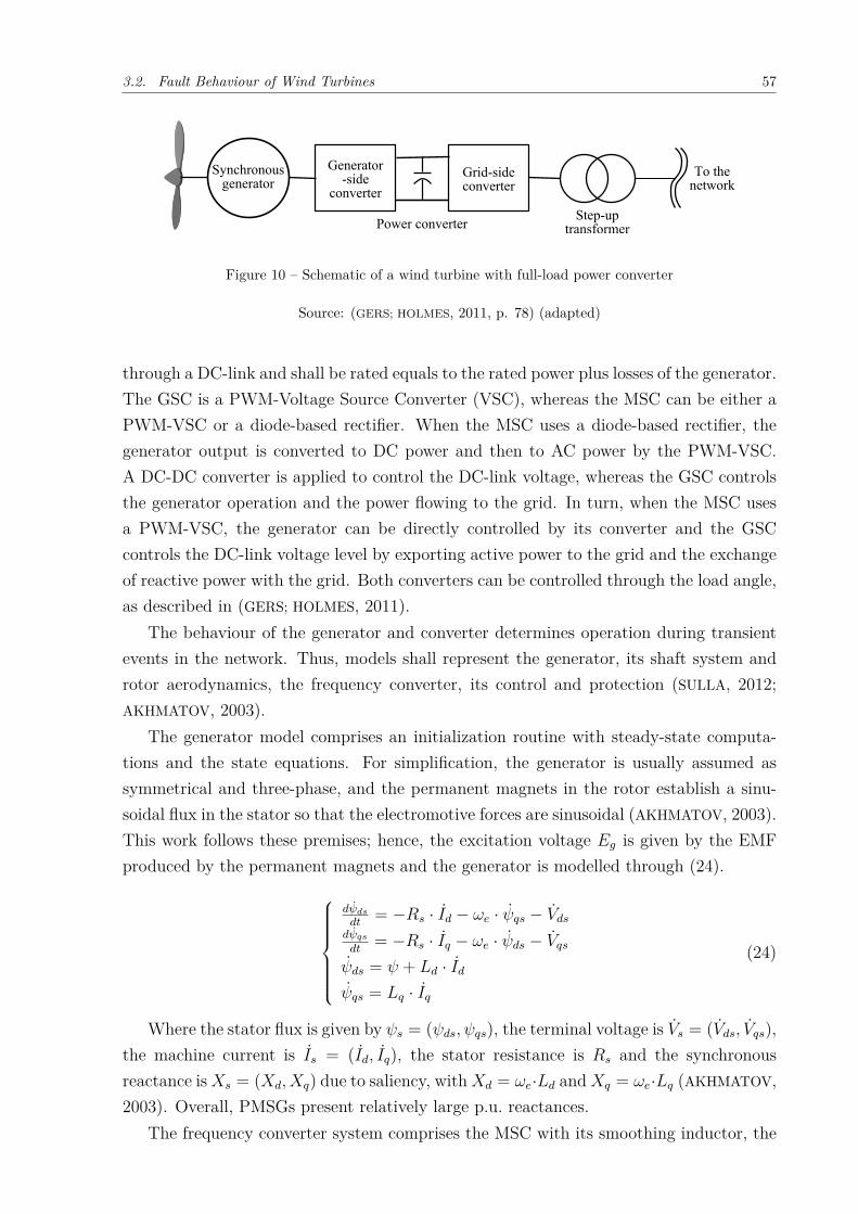
3.2. Fault Behaviour of Wind Turbines 57
Synchronousgenerator
Step-uptransformer
Generator-side
converter
To thenetwork
Grid-side converter
Power converter
Figure 10 – Schematic of a wind turbine with full-load power converter
Source: (GERS; HOLMES, 2011, p. 78) (adapted)
through a DC-link and shall be rated equals to the rated power plus losses of the generator.The GSC is a PWM-Voltage Source Converter (VSC), whereas the MSC can be either aPWM-VSC or a diode-based rectifier. When the MSC uses a diode-based rectifier, thegenerator output is converted to DC power and then to AC power by the PWM-VSC.A DC-DC converter is applied to control the DC-link voltage, whereas the GSC controlsthe generator operation and the power flowing to the grid. In turn, when the MSC usesa PWM-VSC, the generator can be directly controlled by its converter and the GSCcontrols the DC-link voltage level by exporting active power to the grid and the exchangeof reactive power with the grid. Both converters can be controlled through the load angle,as described in (GERS; HOLMES, 2011).
The behaviour of the generator and converter determines operation during transientevents in the network. Thus, models shall represent the generator, its shaft system androtor aerodynamics, the frequency converter, its control and protection (SULLA, 2012;AKHMATOV, 2003).
The generator model comprises an initialization routine with steady-state computa-tions and the state equations. For simplification, the generator is usually assumed assymmetrical and three-phase, and the permanent magnets in the rotor establish a sinu-soidal flux in the stator so that the electromotive forces are sinusoidal (AKHMATOV, 2003).This work follows these premises; hence, the excitation voltage 𝐸𝑔 is given by the EMFproduced by the permanent magnets and the generator is modelled through (24).
⎧⎪⎪⎪⎪⎪⎪⎨⎪⎪⎪⎪⎪⎪⎩
𝑑��𝑑𝑠
𝑑𝑡= −𝑅𝑠 · 𝐼𝑑 − 𝜔𝑒 · ��𝑞𝑠 − ��𝑑𝑠
𝑑��𝑞𝑠
𝑑𝑡= −𝑅𝑠 · 𝐼𝑞 − 𝜔𝑒 · ��𝑑𝑠 − ��𝑞𝑠
��𝑑𝑠 = 𝜓 + 𝐿𝑑 · 𝐼𝑑��𝑞𝑠 = 𝐿𝑞 · 𝐼𝑞
(24)
Where the stator flux is given by 𝜓𝑠 = (𝜓𝑑𝑠, 𝜓𝑞𝑠), the terminal voltage is ��𝑠 = (��𝑑𝑠, ��𝑞𝑠),the machine current is 𝐼𝑠 = (𝐼𝑑, 𝐼𝑞), the stator resistance is 𝑅𝑠 and the synchronousreactance is𝑋𝑠 = (𝑋𝑑, 𝑋𝑞) due to saliency, with𝑋𝑑 = 𝜔𝑒·𝐿𝑑 and𝑋𝑞 = 𝜔𝑒·𝐿𝑞 (AKHMATOV,2003). Overall, PMSGs present relatively large p.u. reactances.
The frequency converter system comprises the MSC with its smoothing inductor, the

58 Chapter 3. Review of modelling distributed generation and load technologies
GSC and the DC-link connection between both sides. The MSC injects the current𝐼1 = 𝑃𝑔
𝑈𝑑𝑐into the DC-link with voltage 𝑈𝑑𝑐. The current from the another side of the DC-
link is given by 𝐼2 = 𝑃𝑔𝑐
𝑈𝑑𝑐, with 𝑃𝑔𝑐 = 𝑃𝑠 + 𝑃𝑙𝑜𝑠𝑠𝑒𝑠, 𝑃𝑠 equals to the active power supplied
to the power system and 𝑃𝑙𝑜𝑠𝑠𝑒𝑠 equals to the power losses in the GSC. In steady-stateoperation and under the assumption of no power losses in the DC-link, 𝑃𝑔𝑐 = 𝑃𝑔 and 𝑈𝑑𝑐is constant and provides the initial condition of the DC-link, 𝑈𝑑𝑐(0). However, when adisturbance occurs, the stationary power equality between 𝑃𝑔𝑐 and 𝑃𝑔 is broken, then acurrent 𝐼𝑐 = 𝐼1 − 𝐼2 starts flowing through the capacitor and causes voltage fluctuationson the DC-link voltage, according to (25) (AKHMATOV, 2003)
𝑈𝑑𝑐(𝑡) =√𝑈2𝑑𝑐(0) + 2
𝐶·
∫(𝑃𝑔(𝜏) − 𝑃𝑔𝑐(𝜏)) · 𝑑𝜏 (25)
The current flowing through the GSC can be calculated through (26):
⎧⎪⎪⎪⎪⎪⎪⎨⎪⎪⎪⎪⎪⎪⎩
𝑑��𝑑𝑠
𝑑𝑡= −𝑅𝑠 · 𝐼𝑑 − 𝜔𝑒 · ��𝑞𝑠 −
(��𝑑𝑐 − ��𝑑𝑠
)𝑑��𝑞𝑠
𝑑𝑡= −𝑅𝑠 · 𝐼𝑞 − 𝜔𝑒 · ��𝑑𝑠 −
(��𝑞𝑐 − ��𝑞𝑠
)��𝑑𝑠 = 𝑋𝑠 · 𝐼𝑑��𝑞𝑠 = 𝑋𝑠 · 𝐼𝑞
(26)
With ��𝑠 = (��𝑑𝑠, ��𝑞𝑠) equals to the grid voltage and ��𝑐 = (��𝑑𝑐, ��𝑞𝑐) equals to the voltagegenerated by the GSC. Analogously, the grid voltage ��𝑔 = (��𝑑, ��𝑞) is controlled by theMSC.
The voltage exchanged between the GSC and the grid is given by 𝑆𝑠 = 𝑃𝑠 + 𝑗 ·𝑄𝑠 =��𝑠 · 𝐼𝑠* and the power losses in the GSC are given by 𝑃𝑙𝑜𝑠𝑠𝑒𝑠 = 𝑅𝑠 · 𝐼2
𝑠 .Since the converter determines the operation of the wind turbine during transients,
its protective system has to be evaluated. Overall, the relay settings of the converter areprovided by the wind turbine manufacturer; otherwise, they can be evaluated according tothe operation principles. The blocking time of the converter controlled by IGBT-switchescan be of a few milliseconds. Besides, the generator protection at faults usually focuses onprotection against over-current in the stator windings and thermal overload. The PMSGis separated from the fault in the grid by the converter with the DC-link. Hence, gridfaults may not damage the PMSG with demagnetization of the magnets. Nonetheless,the converter control has to be designed to reduce stress from the grid on the generator.
In principle, full-load power converters can be disconnected instantaneously duringgrid disturbances without contributing to fault currents at all (THIRINGER; PETERSSON;
PETRU, 2003; PETRU; THIRINGER, 2002); in this case, they behave as an open circuit.Alternatively, they can be controlled so as to produce a certain amount of active andreactive power; in this case, the reactive power can be controlled independently by theGSC, whereas the active power control have to comply with the mechanical parametersof the wind turbine (THIRINGER; PETERSSON; PETRU, 2003).

3.2. Fault Behaviour of Wind Turbines 59
During a grid fault, the converter shall operate without protective tripping (AKHMA-
TOV, 2003). When the risk of converter blocking at grid faults is indicated, blocking-and-restarting features must be suggested for the frequency converters so that the windturbine can operate without interruption. Thereby, after the fault clearance, the fre-quency converter shall restart so that the generator can supply active power to the gridcontinuously.
In contrast, when the DC-link voltage exceeds the tripping limit, the MSC stopsswitching, then its IGBT-switches open and the PMSG checks into the DC-link capacitorthroughout the diode-bridge, whereas the GSC continues to operate. In this condition, thedynamic behaviour of the generator plus its converter is characterized by two conflictingprocesses (AKHMATOV, 2003): charge of the DC-link capacitor throughout the diode-bridge from the generator and discharge of the DC-link capacitor by the GSC. TheDC-link capacitor discharges due to the active power supply from the GSC to the grid.It can be eliminated by setting the active current reference of the GSC to zero, so thatthe capacitor charges rapidly and the voltage reaches the generator excitation voltage.Then, the stator-winding current decays to zero and the accumulated magnetizing energyis transferred whilst the DC-link capacitor is charging.
The short-circuit behaviour is mainly determined by the GSC control strategy. Hence,it is specific to each wind turbine and field measurements are the only practical way to geta realistic picture of the fault behaviour of this concept. Overall, the wind turbine does notcontribute to the short-circuit power because the full-load converters limit the current fedinto the fault to the rated current of the converter or slightly above of it. Thus, the windturbine can be approximated as a constant current source. For severe fault events, theconverter switching may be interrupted during the fault period (KANELLOS; KABOURIS,2009; SULLA, 2012; MORREN; HAAN, 2007; TEODORESCU; LISERRE; RODRÍGUEZ, 2010).
Voltage dips do not impact directly the generator dynamics because the GSC is able toride through the fault and supply reactive current. The generator may over-speed withincertain limits to store part of the mechanical power as kinetic energy, whilst pitch controlis applied to reduce the mechanical power. However, a chopper resistance is requestedto dissipate the input power and keep the DC-link voltage within acceptable levels undersevere fault conditions. Alternatively, control techniques may be applied to improve thedynamic performance and avoid temporary over-current (SULLA, 2012).
3.2.2 Wind farms
A wind farm typically includes a number of wind turbines. A scheme is illustratedin Figure 11.
Wind turbines are unlikely to produce the same output power in a wind farm due tothe shadowing effects among them with respect to the incoming wind; additionally, theremay be slight voltage variations throughout the internal cable network of the wind farm.

60 Chapter 3. Review of modelling distributed generation and load technologies
WT3
WT12
WT9
WT6
WT2
WT11
WT8
WT5
WT1
WT10
WT7
WT4
To the
grid
PCC
Figure 11 – Single-line diagram of a detailed wind farm model with 12 wind turbines
Source: (SULLA, 2012, p. 78) (adapted)
Thus, it is important to consider that the wind turbines may be at different operatingpoints with different parameters and relay settings to evaluate the fault behaviour of awind farm.
Wind farms can be modelled in detail, with representation of each turbine in the farm,their no-load capacitor, the transformer connecting the wind turbine to the internal cablenetwork and sufficient detailed information on the wind farm (AKHMATOV, 2003). Alter-natively, reduced models in which the wind farm is represented by a rescaled equivalentmay be applied in special conditions, when the differences between the operating pointsof the wind turbines are not too large (VITTAL; AYYANAR, 2012; LINDGREN; SVENSSON;
GERTMAR, 2012). The complete model of wind turbines is required for actual investiga-tion of the control features into individual wind farms, whereas the reduced model maybe successfully applied for investigating the collective response of the wind farm undershort-circuits (VITTAL; AYYANAR, 2012; LINDGREN; SVENSSON; GERTMAR, 2012). Al-ternatively, when the wind distribution is irregular over the area where the wind farmis, a multi-machine equivalent approach can be applied to represent the wind farm by areduced number of re-scaled turbines at the same operating points.
Some simplifying assumptions to calculate the parameters of a typical wind farmpresent negligible effect on the results, as follows (KANELLOS; KABOURIS, 2009; JAUCH et
al., 2007):
– the groups of wind turbines contain the same number of wind turbines;
– adjacent wind turbines and groups of wind turbines are placed at equal distances;
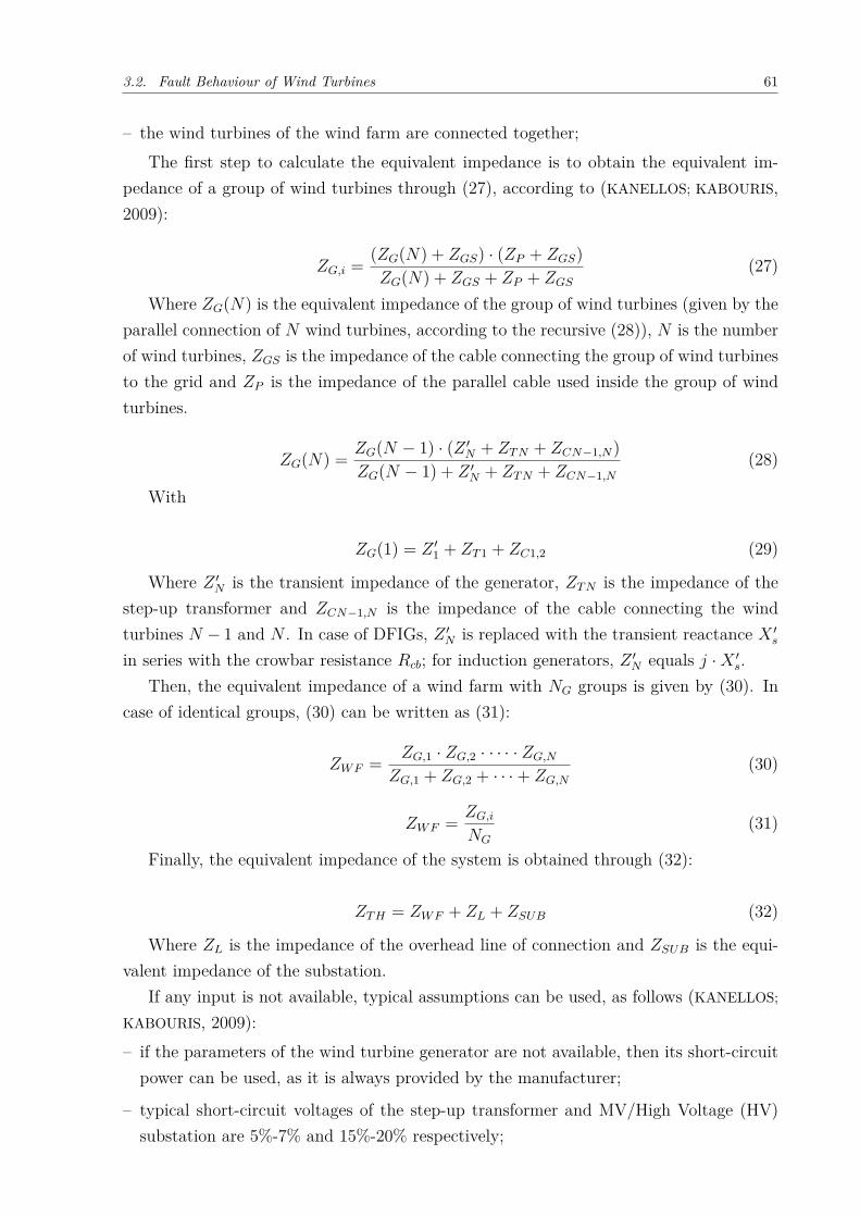
3.2. Fault Behaviour of Wind Turbines 61
– the wind turbines of the wind farm are connected together;The first step to calculate the equivalent impedance is to obtain the equivalent im-
pedance of a group of wind turbines through (27), according to (KANELLOS; KABOURIS,2009):
𝑍𝐺,𝑖 = (𝑍𝐺(𝑁) + 𝑍𝐺𝑆) · (𝑍𝑃 + 𝑍𝐺𝑆)𝑍𝐺(𝑁) + 𝑍𝐺𝑆 + 𝑍𝑃 + 𝑍𝐺𝑆
(27)
Where 𝑍𝐺(𝑁) is the equivalent impedance of the group of wind turbines (given by theparallel connection of 𝑁 wind turbines, according to the recursive (28)), 𝑁 is the numberof wind turbines, 𝑍𝐺𝑆 is the impedance of the cable connecting the group of wind turbinesto the grid and 𝑍𝑃 is the impedance of the parallel cable used inside the group of windturbines.
𝑍𝐺(𝑁) = 𝑍𝐺(𝑁 − 1) · (𝑍 ′𝑁 + 𝑍𝑇𝑁 + 𝑍𝐶𝑁−1,𝑁)
𝑍𝐺(𝑁 − 1) + 𝑍 ′𝑁 + 𝑍𝑇𝑁 + 𝑍𝐶𝑁−1,𝑁
(28)
With
𝑍𝐺(1) = 𝑍 ′1 + 𝑍𝑇1 + 𝑍𝐶1,2 (29)
Where 𝑍 ′𝑁 is the transient impedance of the generator, 𝑍𝑇𝑁 is the impedance of the
step-up transformer and 𝑍𝐶𝑁−1,𝑁 is the impedance of the cable connecting the windturbines 𝑁 − 1 and 𝑁 . In case of DFIGs, 𝑍 ′
𝑁 is replaced with the transient reactance 𝑋 ′𝑠
in series with the crowbar resistance 𝑅𝑐𝑏; for induction generators, 𝑍 ′𝑁 equals 𝑗 ·𝑋 ′
𝑠.Then, the equivalent impedance of a wind farm with 𝑁𝐺 groups is given by (30). In
case of identical groups, (30) can be written as (31):
𝑍𝑊𝐹 = 𝑍𝐺,1 · 𝑍𝐺,2 · · · · · 𝑍𝐺,𝑁𝑍𝐺,1 + 𝑍𝐺,2 + · · · + 𝑍𝐺,𝑁
(30)
𝑍𝑊𝐹 = 𝑍𝐺,𝑖𝑁𝐺
(31)
Finally, the equivalent impedance of the system is obtained through (32):
𝑍𝑇𝐻 = 𝑍𝑊𝐹 + 𝑍𝐿 + 𝑍𝑆𝑈𝐵 (32)
Where 𝑍𝐿 is the impedance of the overhead line of connection and 𝑍𝑆𝑈𝐵 is the equi-valent impedance of the substation.
If any input is not available, typical assumptions can be used, as follows (KANELLOS;
KABOURIS, 2009):– if the parameters of the wind turbine generator are not available, then its short-circuit
power can be used, as it is always provided by the manufacturer;
– typical short-circuit voltages of the step-up transformer and MV/High Voltage (HV)substation are 5%-7% and 15%-20% respectively;

62 Chapter 3. Review of modelling distributed generation and load technologies
– a typical MV overhead line can be considered for connection of the wind farm to thesubstation and the thermal limit of the conductor can be used to determine the numberof parallel circuits;
– an average distance of 300 m between adjacent turbines can be considered;
– typical XLPE cables, whose cross section depends on the size of the wind turbine, canbe assumed for internal wiring.
When the wind farm is composed of wind turbines equipped with full-load powerconverters, it can be modelled as a constant current source (KANELLOS; KABOURIS, 2009).
In accordance with (JAUCH et al., 2007), transient faults in weak parts of the systemimpact locally the system voltage, as local voltage dips are hardly ever noticed in otherparts of the system. However, it produces torsional oscillations in the drive trains ofthe wind turbines, which result in power fluctuations that propagate through the systemand may lead synchronous generators to exhibit frequency oscillations. Therefore, a highpenetration level of fixed-speed turbines leads to strong power and frequency fluctuationsin the grid.
In the case of induction generators, there is no synchronizing torque and almost nointeraction between the wind turbine shafts and the generators through the electricalnetwork. Thereby, the wind turbines at the same operating point can be simply addedand represented as a reduced equivalent. In particular, the coherent response can beobtained when the wind turbine data are identical, the short-circuit impedances seenfrom the terminals of the different wind turbines within the wind farm are practically ofthe same value and mutual interactions are absent (AKHMATOV, 2003).
If a group of wind turbines have different mechanical parameters, their natural fre-quencies (and shaft torsional modes) will also differ and the risk of mutual oscillations willarise at grid disturbances. The wind turbines start responding to the fault in functionof their natural frequencies, but in absence of synchronizing torque, the fluctuations inelectrical and mechanical parameters will eliminate each other. The resulting dynamicbehaviour is smoother than in case of wind turbines with identical parameters, with redu-ced voltage oscillations (AKHMATOV, 2003). Thus, it may be preferred to combine windturbines with different parameters within a large wind farm.
3.2.3 Grid-fault ride-through requirements
Requirements on GFRT capability are related to technology, protection and controlof wind turbines, generators and power electronics, as well as design and sizing of auxi-liary equipment. Overall, they still represent a challenge for wind turbine manufacturers(TEODORESCU; LISERRE; RODRÍGUEZ, 2010). Essentially, GFRT parts of national gridcodes specify the limiting conditions for a wind turbine to remain connected to the gridduring a voltage dip by curves of the voltage dip in function of time. Voltage dips that

3.3. Fault Behaviour of Photovoltaic Systems 63
follow a grid fault and are cleared in normal conditions are expected to be above thesecurves. The voltage dip duration depends on the speed of fault clearance, which dependson the protection system. Voltage versus time curves from some European national gridcodes can be found in (SULLA, 2012; IOV et al., 2007; TEODORESCU; LISERRE; RODRÍGUEZ,2010).
3.3 Fault Behaviour of Photovoltaic Systems
3.3.1 Basic concepts of photovoltaic systems
Photovoltaic (PV) systems have been deployed at increasing levels in power distri-bution systems. Consequently, adequate models of panels and inverters are required fordifferent grid impact studies.
A typical grid-connected PV system may be represented by a variable voltage in-put connected to a DC-DC converter with Maximum Power Point Tracking (MPPT), aregulated DC-link and a DC-AC three- or single-phase inverter.
PV cells are connected in series-parallel arrangements to produce a particular amountof power at a given voltage level, as a typical PV cell produces less than 2 [W] at 0.5 [V](DC). Single PV cells are connected to build modules that in turn are connected to buildarrays. A module may have a power output from a few to hundreds of watts, whereas thepower output of an array may vary from hundreds to millions of watts (WANG, 2006).
PV systems can be either stand-alone or grid-connected. In both cases, the DC outputgenerated by the PV cells is converted to AC power through inverters, which resultsin non-sinusoidal current waveforms. Grid-interfaced inverters are equipped with filtersin order to attenuate lower and higher frequency components and smooth the outputwaveform (APRILIA et al., 2012).
The inverter is the key element of a grid-connected PV system. Its main functionis to convert the DC output power of the PV panels to AC grid-synchronized power.Depending on the configuration of the PV system, the inverter can be classified as in(TEODORESCU; LISERRE; RODRÍGUEZ, 2010):
– module-integrated, typically between 50 and 400 [W], for very small PV plants;
– string, typically between 0.4 and 2 [kW], for small roof-top plants with panels connectedin one string;
– multi-string, typically between 1.5 and 6 [kW], for medium roof-top plants with panelsin one or two strings;
– multi central, typically above 6 [kW] with three-phase topology and modular design forlarger roof-top or smaller power plants;

64 Chapter 3. Review of modelling distributed generation and load technologies
– central, typically between 100 and 1000 [kW] with three-phase topology and modulardesign for large power plants.
Inverters are more complex in a PV system than in a motor drive with regards tohardware and functionality. Some features of a PV inverter include, the grid connectionfilter, grid disconnection relay, DC switch and functions such as the MPPT, anti-islanding,grid synchronization and data logger (TEODORESCU; LISERRE; RODRÍGUEZ, 2010).
3.3.2 Grid requirements for response to abnormal conditions
PV systems have to comply with a number of standard requirements in order to ensuresafety and seamless transfer of electrical energy to the grid. Local regulations imposedby grid operators apply in most of the countries. Some international bodies have alsodeveloped worldwide standards for grid requirements, such as Institute of Electrical andElectronic Engineers (IEEE), International Electrotechnical Comission (IEC), DeutscheKommission Elektrotechnik (DKE) and so on.
Overall, these regulations stipulate disconnection time limits in function of voltageand frequency variations (TEODORESCU; LISERRE; RODRÍGUEZ, 2010) and conditions forreconnection. The disconnection times refer to the interval between the occurrence of theabnormal condition and the cease to energize the utility line, in order to ride throughshort-term disturbances to avoid excessive nuisance tripping, particularly in weak-gridsituations.
Grid requirements have a significant impact on the design and performance of theinverters. The equipment must be disconnected from the grid in case of abnormal con-ditions, so as not to be damaged and to ensure safety for the general public, while theinverter controller shall remain connected to the utility to sense the conditions for recon-nection.
3.3.3 Modelling photovoltaic systems
There is very little standardization in modelling PV generation in power distributionsystems. Most of the efforts have been based on analytical methods that do not reflecttheir response to variable conditions in irradiation, grid voltage and frequency. Alterna-tively, the assumption that the PV system behaves as an active load injecting energy intothe power system may be convenient, as well as empirical models based on experimentalresults and field measurements. Although detailed models (for example, including thePV array, MPPT algorithm and power electronics) may be suitable to evaluate a parti-cular PV system, the precision is generally lost when wide aggregation is needed. Hence,a simple, practical and faithful PV system model has to be established together withthe aggregate representation of dynamic and static loads within the distribution networkmodel (LESIEUTRE, 2008).

3.3. Fault Behaviour of Photovoltaic Systems 65
Io +
_Vd VoRp
Rs
+
_
IpId
I
Figure 12 – Equivalent electrical circuit of a single photovoltaic cell
Source: (FARRET; oES, 2006, p. 132) (adapted)
A few decades ago, converter-based generation did not contribute to a significant shareof active power generation to the system. They used to be immediately disconnected fromthe grid after a fault had been detected, because their reactive current contribution tothe short circuit was small compared to the traditional synchronous machines. However,due to the increasing penetration levels of converter-based generation, the disconnectionmay adversely impact the system stability, so this practice is no longer feasible.
New guidelines and regulations pose that converter-based power generation shall becapable to ride through faults, by remaining connected to the grid as long as the faultcondition does not exceed certain limits. Whereas they remain connected, their controlsystem has to respond fast to voltage changes by adjusting the reactive current contribu-tion along a given characteristic. Thus, the short-circuit contribution of converters hasto be taken on board.
The power converter limits the reactive current magnitude up to the rated currentat nominal apparent power. Therefore, the synchronous machine model will not provideaccurate results, as its transient short circuit contribution can reach 20 times the nominalvalue, according to 3. Besides, the fault current contribution with use of power convertersis independent of the fault distance and resembles a synchronous machine only within arange of voltage drop values at the converter terminals.
The equivalent electric circuit of a single PV cell is shown in Figure 12. The outputcurrent can be calculated by means of (FARRET; oES, 2006; CUK et al., 2011; APRILIA et
al., 2012):
𝐼𝑜 = 𝐼𝜆 − 𝐼𝑑 − 𝐼𝑝 (33)
Where 𝐼𝜆 is the photon current, proportional to the light intensity and dependent onthe light wavelength; 𝐼𝑑 is the Shockley temperature-dependent diode current; and 𝐼𝑝 isthe PV cell leakage current.
The parameters of the photon current are related to the cell short-circuit current and tothe cell open-circuit voltage, obtained from the current-voltage (I-V) characteristic curve.Moreover, if the photon current is known for certain standard illumination intensity 𝐿𝑠
and a prescribed value of 𝐼𝜆,𝑜, it is possible to obtain the photon current approximately

66 Chapter 3. Review of modelling distributed generation and load technologies
for another intensity 𝐿 through:
𝐼𝜆 = 𝐿
𝐿𝑠· 𝐼𝜆,𝑜 (34)
The Shockley diode current is given by:
𝐼𝑑 = 𝐼𝑠 ·[𝑒
𝑞·𝑉𝑑𝜂·𝑘·𝑇 − 1
](35)
Where 𝐼𝑠 is the reverse saturated current of the diode, 𝑘 is the Boltzmann constant,𝑞 is the electron charge, 𝑉𝑑 is the diode voltage, 𝜂 is an empirical constant and 𝑇 is theabsolute temperature (FARRET; oES, 2006).
In turn, the leakage current is given by:
𝐼𝑝 = 𝑉𝑑𝑅𝑝
(36)
The internal losses across the diode can be represented by a parallel resistance (ty-pically between 200 and 800 [Ω]), whereas the manufacturing quality of the PV cell canbe reflected by a small series resistance between the photon current source and the loadacross the terminals (up to 0.1 [Ω]).
Writing the diode voltage in function of the load resistance 𝑅𝐿 , as in (37), the outputcurrent can be written as in (38):
𝑉𝑑 = 𝐼𝑜 · (𝑅𝑠 +𝑅𝐿) = 𝑉𝑜 ·(
1 + 𝑅𝑠
𝑅𝐿
)(37)
𝐼𝑜 = 𝑅𝑝
𝑅𝑝 +𝑅𝑠 +𝑅𝐿
·[𝐼𝜆 − 𝐼𝑠 ·
(𝑒
𝑞·𝑉𝑑𝜂·𝑘·𝑇 − 1
)](38)
When a group of PV cells is integrated, the cells are assumed to be identical. Suchpractice is reasonable, as the individual cells are manufactured with very similar charac-teristics to avoid circulation of internal currents among the cells. Hence, the assumptionsbelow are acceptable:
⎧⎪⎪⎪⎪⎪⎪⎪⎪⎪⎨⎪⎪⎪⎪⎪⎪⎪⎪⎪⎩
𝐼𝜆,1 = 𝐼𝜆,2 = · · · = 𝐼𝜆,𝑛
𝐼𝑑,1 = 𝐼𝑑,2 = · · · = 𝐼𝑑,𝑛
𝑉𝑑,1 = 𝑉𝑑,2 = · · · = 𝑉𝑑,𝑛
𝑅𝑠,1 = 𝑅𝑠,2 = · · · = 𝑅𝑠,𝑛
𝑅𝑝,1 = 𝑅𝑝,2 = · · · = 𝑅𝑝,𝑛
(39)
The output voltage and current of a series-connected group are given by (40), where𝑉𝑜,𝑖 and 𝐼𝑜,𝑖 are the average voltage and current in an individual cell.
⎧⎨⎩ 𝑉𝑜 = 𝑛 · 𝑉𝑜,𝑖𝐼𝑜 = 𝐼𝑜,𝑖
(40)
3.4. Fault Behaviour of Fuel Cells 67
In turn, the output voltage and current of a parallel-connected group are given by(41):
⎧⎨⎩ 𝑉𝑜 = 𝑉𝑜,𝑖
𝐼𝑜 = 𝑛 · 𝐼𝑜,𝑖(41)
A PV system at the distribution grid might be considered as a negative power elec-tronic load. However, its principles of control and operation differ from typical powerelectronic loads that essentially operate near constant power at unity power factor for awide voltage range (LESIEUTRE, 2008). Moreover, the power converters of a PV systemapply a MPPT function in the DC-DC converter module. Therefore, the PV modellingillustrated in 12 is not strictly load modelling.
3.4 Fault Behaviour of Fuel Cells
Fuel cell DG systems have many advantages, such as high efficiency, zero or low ofpollutant gases and flexible modular structure. They are invaluable sources to providereliable power at steady state, but due to their slow internal electrochemical and ther-modynamic responses, their response to electrical load transients is not as fast as desired.Hence, their short-circuit behaviour has to be analysed.
This section presents the analytical models of fuel cells related to operation duringgrid disturbances, including details with respect to the power converter configurationsand controllers.
3.4.1 Basic concepts
Fuel cells are static energy conversion devices that convert the chemical energy of thefuel into DC electrical energy (WANG, 2006). These components consist of two electrodes(anode and cathode) and an electrolyte layer in the middle. The electrolyte layer is a goodconductor for ions either positive or negative charged and can be either solid or liquid.The type and chemical properties of the electrolyte in use are crucial to the operatingcharacteristics.
Typically, the fuel is fed continuously to the anode, whereas the oxidant is fed continu-ously to the cathode. The most commonly used fuel is hydrogen, whilst the most commonoxidant is oxygen or air. The electrochemical reactions take place at the electrodes.
Among the different types of fuel cells, the most likely to be used for DG applicationsaccording to (WANG, 2006) are:– Solid oxide fuel cell (SOFC): based on a negative-ion conductive electrolyte, it operates
at high temperatures (600-1000 Celsius degrees), converts chemical energy into electricalenergy at high efficiency (up to 65%) and the solid nature of the fuel eliminates corrosionand management concerns related to the liquid electrolyte;

68 Chapter 3. Review of modelling distributed generation and load technologies
– Polymer electrolyte membrane fuel cell (PEMFC): with a sandwich-like structure and aTeflon-like membrane that is an excellent conductor of protons and insulator of electronsbetween the two electrodes, it presents high power density, high efficiency (40-45%) andlower operating temperature (60-80 Celsius degrees) (WANG, 2006); and
– Molten carbonate fuel cell (MCFC): using a mixture of alkali metal carbonate aselectrolyte, it operates at high temperatures (600-700 Celsius degrees), when the saltmixture is in liquid phase, and can achieve efficiency in the range of 50-60% before heatrecovery and exceed 70% with heat recovery.
3.4.2 Dynamic models for fuel cells
Fuel cells are usually connected to the grid through power electronics. However, theexchange of information between fuel cell manufacturers and power electronic interface de-signers is often limited. As a consequence, the former model the power electronic interfaceas an equivalent impedance, whereas the latter represent the fuel cell as a constant voltagesource with a series resistance. These approaches may lead to inaccurate results whenfuel cells and power electronic converters are connected, so it is important to understandhow these components impact each other (WANG, 2006).
Typically, the fuel cell is connected to the power system through a DC-AC converterequipped with voltage- and power-control loops (JAGADURI; RADMAN, 2007). In addition,a battery is necessary to provide voltage support and reactive power compensation. Fuelcells produce DC voltage outputs and present slow transient response and output powerramping, so they cannot follow loads effectively. They serve as a stationary power gene-rator that generates power on its own. Among the types commonly used, the PEMFChas the fastest transient response.
The inverter applies PWM to turn the DC voltage into a controllable AC voltage withfundamental frequency, according to:
��𝐴𝐶 = 𝑚 · 𝑉𝐹𝐶 · (1 𝛿) (42)
Where 𝑉𝐹𝐶 is the DC voltage at the fuel cell terminals, 𝑚 is the amplitude modulationindex of the converter, and 𝛿 represents the firing angle of the power converter with respectto the reference bus voltage (JAGADURI; RADMAN, 2007). The output voltage of the fuelcell stack can be calculated through:
𝑉𝐹𝐶 = 𝑁𝑐𝑒𝑙𝑙 · 𝑉𝑐𝑒𝑙𝑙 (43)
In turn, the battery added to make up for the slow transients can be modelled asan ideal voltage source, as its internal resistance is very small. The equivalent circuit is

3.5. Fault Behaviour of Gas Micro-turbines 69
Idc+
_
EFC
VFC
XFC
+
_
Figure 13 – Equivalent electrical circuit of a fuel cell
Source: (JAGADURI; RADMAN, 2007, p. 5) (adapted)
illustrated in Figure 13:⎧⎨⎩ 𝐼 = 𝑌𝐹𝐶 · (𝐸𝐹𝐶 − 𝑉𝐹𝐶)𝑌𝐹𝐶 = 1
𝑗·𝑋𝐹 𝐶= 𝑗 ·𝐵𝐹𝐶
(44)
(44) can be written in terms of real and imaginary components (system referenceframe), as:
⎡⎣ 𝐼𝑟𝑒
𝐼𝑖𝑚
⎤⎦ =⎡⎣ 0 −𝐵𝐹𝐶
−𝐵𝐹𝐶 0
⎤⎦ ·
⎡⎣ ��𝑟𝑒
��𝑖𝑚
⎤⎦ −
⎡⎣ 𝐵𝐹𝐶 · �� ′𝑖𝑚
−𝐵𝐹𝐶 · �� ′𝑟𝑒
⎤⎦ (45)
Although the battery presents an extremely high initial density of current (ZAVALIS;
BEHM; LINDBERGH, 2012), the current over time does not differ considerably from thefully charged case. More current is produced and the temperature rises faster when theelectrode area is increased.
3.5 Fault Behaviour of Gas Micro-turbines
Gas micro-turbines used for DG applications have been deployed at increasing levelsin power distribution systems. Hence, their impact on the grid has to be represented andevaluated properly. This section presents the concepts of gas micro-turbines commonlyused and the analytical models required for operation during grid disturbances, includingdetails with respect to the power converters, as follows.
3.5.1 Basic concepts of gas micro-turbines
The main components of a gas turbine are compressor, combustor and turbine. Theair is pressurized in the compressor before entering the combustor, where it is mixed withthe fuel injected. Then the mixture is ignited and mechanical power is produced whenthe hot combustion gases flow and expand through the turbine. The gas turbine drives asynchronous generator, where part of the power produced is converted to electric power(JAGADURI; RADMAN, 2007). Therefore, the electrical characteristics of the gas turbineare determined by the synchronous machine.

70 Chapter 3. Review of modelling distributed generation and load technologies
Idc+
_
EGT
VGT
XGT
+
_
Figure 14 – Equivalent electrical circuit of a gas micro turbine
Source: (JAGADURI; RADMAN, 2007, p. 5) (adapted)
3.5.2 Dynamic models for gas micro-turbines
A two-axis model is assumed for the gas turbine (JAGADURI; RADMAN, 2007). Accor-ding to the phasor diagram, �� is the voltage induced by the field current 𝐼𝑓 and �� ′ is thenet voltage induced by 𝐼𝑓 and the armature reaction. In the d-q frame of reference, thesteady-state characteristics of the gas turbine at its terminals are given by:
⎧⎨⎩ �� ′ = ��𝑞 +𝑅 · 𝐼𝑞 −𝑋 ′𝑑 · 𝐼𝑑
0 = ��𝑑 +𝑅 · 𝐼𝑑 −𝑋𝑞 · 𝐼𝑞(46)
Ignoring the resistance 𝑅, the equations can be written as:⎡⎣ 𝐼𝑞
𝐼𝑑
⎤⎦ =⎡⎣ 0 − 1
𝑋𝑞
1𝑋𝑑
0
⎤⎦ ·
⎡⎣ ��𝑞
��𝑑
⎤⎦ −
⎡⎣ 0��′
𝑋′𝑑
⎤⎦ (47)
The d-q components of the gas turbine voltage and current are transformed to thesystem reference frame through the transformation matrix given by (48):
[𝑇 ] =⎡⎣ cos(𝛿) sin(𝛿)
− sin(𝛿) cos(𝛿)
⎤⎦ (48)
Hence,⎡⎣ 𝐼𝑑
𝐼𝑞
⎤⎦ = [𝑇 ] ·
⎡⎣ 𝐼𝑟𝑒
𝐼𝑖𝑚
⎤⎦ and⎡⎣ 𝑉𝑑
𝑉𝑞
⎤⎦ = [𝑇 ] ·
⎡⎣ ��𝑟𝑒
��𝑖𝑚
⎤⎦ (49)
Substituting (49) in (47):⎡⎣ 𝐼𝑟𝑒
𝐼𝑖𝑚
⎤⎦ = [𝑇 ]−1 ·
⎡⎣ 0 − 1𝑋𝑞
1𝑋𝑑
0
⎤⎦ · [𝑇 ] ·
⎡⎣ ��𝑟𝑒
��𝑖𝑚
⎤⎦ − [𝑇 ]−1 ·
⎡⎣ 0��′
𝑋′𝑑
⎤⎦ (50)
The equivalent circuit is shown in Figure 14.
3.6 Fault Behaviour of Loads
Aggregate loads remain the least certain of the modelled elements in power systems.Loads are highly distributed and quite variable, consequently accurate modelling is very
3.6. Fault Behaviour of Loads 71
difficult and aggregation is the most practical approach to incorporate them in powersystem studies. As the load composition continually changes, even if it was possible toobtain an accurate load model for a certain time period, it would be inaccurate a shortwhile later.
Nonetheless, load composition is very important on the analysis of the power systemdynamic behaviour, as different load types exhibit distinct responses to disturbances. Des-pite that, the overall load composition tends to behave fairly predictably. Model structuresfor large dominant components, such as synchronous generators, are well established, aswell as the procedures to determine the associated parameter values. Conversely, modelsthat represent an aggregation of many elements bring uncertainties related to their overallcomposition. In this context, the next sections describe previous attempts and currentpractices on load modelling.
3.6.1 Previous attempts on load modelling
Most of the load models currently used in power system studies were developed a fewdecades ago and not updated adequately after consecutive changes in the load structure.Although the majority of the power system research and industry acknowledges the im-portance of accurate load modelling, static loads are typically represented by the constantimpedance, current and power models, whereas dynamic loads are commonly representedby the induction motor model. Several unsuccessful attempts to rebuild blackouts in thesimulations have shown the inadequacy of such models.
Historically, loads have been represented with static characteristics, as constant cur-rent for active power and constant impedance for reactive power. Computational limitati-ons used to be the main obstacles to adopt more comprehensive load models. Nowadays,the tools commonly used apply the positive sequence approach in a simplified approach,under the assumptions that only the positive sequence impacts the synchronizing forcesbetween three-phase rotating machines and the behaviour of single-phase loads can beaggregated. However, explicit representation of three-phase and single-phase models maybe desirable to study unbalanced faults; for instance, in load centres with many com-pressor motors for residential air-conditioning and refrigeration, where the response ofload-inertia single-phase motors to unbalanced faults is inconsistent with the positive-sequence approach.
Recently, the interest in load modelling has increased due to the appearance of newload types with improvements in efficiency and controllability. Different non-linear powerelectronic loads are responsible for a significant part of the total demand in the residentialsector (MILANOVIC et al., 2013). On the top of that, the complexity of load compositionsand their hourly and seasonal changes in the real system pose a challenge to accuraterepresentation.

72 Chapter 3. Review of modelling distributed generation and load technologies
A
B
C
D
Electronic
Motors
Load modelcomponents
FeederEquivalent
Transformer
SubstationShunt
{Static
Figure 15 – WECC Composite Load Model
Source: (BRAVO et al., 2010, p. 8) (adapted)
3.6.1.1 WECC Load Modelling Task Force
Wisconsin Energy Conservation Corporation (WECC) has undertaken significant ef-forts to improve dynamic load models and deployed an interim load model with static anddynamic parts. The former accounts for 80% and the latter – a default induction motor– for approximately 20% of the total load connected to a HV bus.
However, the interim load model does not reproduce the observed system response ofdelayed voltage recovery events, since it does not represent accurately the behaviour ofsmall induction motors used in air conditioner compressors. For instance, the wide-spreadstalling of residential single-phase air conditioners, which can occur in less than 2 cycles(i.e. faster than the fault clearance) draws a locked rotor current 4-6 times the rated valueand results in voltage depression in the distribution and sub-transmission levels (WECC-
MVWG, 2012). Hence, stalled air conditioners can be seen as a wide-area high impedancefault.
Afterwards, further advances of computing capability allowed the development of acomposite load model with a more realistic structure, which consists of the following(WECC-MVWG, 2012; KOSTEREV; MEKLIN, 2006):
a) distribution equivalent data: transformer, feeder equivalent and end-use loads pla-ced at the low-voltage bus;
b) model component data: reactance, time constants, inertia and driven load of mo-tors, voltage and frequency sensitivity of static loads;
c) load model composition: fractions of the load assigned to each model component.The composite load model, schematised in Figure 15, takes into account the distance
between the transmission bus and the end-users, includes separate impedances of thesubstation transformer and distribution feeder equivalent and separate capacitors at bothfeeder ends. The capacitor between transformer and feeder impedances provides the

3.6. Fault Behaviour of Loads 73
difference in transformer and feeder reactive flows and a reference point for the transformervoltage regulator. Besides, it includes system and feeder protection and is able to trippart of the equivalent feeder and load (KOSTEREV; MEKLIN, 2006).
The composite load model has a wide range of load dynamics observed in reality.WECC utilities have tested a large variety of end-uses, such as residential and commer-cial air-conditioners, fans, pumps, residential appliances, lighting, computers, variablefrequency drives, non-interruptible power supplies etc. in order to develop dynamic loadmodels (WECC-MVWG, 2012).
Static models represent resistive, lighting, electronic loads and small appliances. Resis-tive loads, such as space heating, incandescent lighting, water heating and cooking, havebeen phasing out, whereas electronic loads, such as fluorescent lighting, electronic drivesand chargers, light-inertia compressor motors in air conditioners and heat pumps, havebeen increasing their penetration level. The former are voltage sensitive, while the latterbehave mostly as constant power loads with respect to voltage and frequency variationsand are susceptible to voltage stability issues and power oscillations. Light-inertia single-phase compressor motors are prone to stall when voltage drops below 60% in 3 cycles orless; in this case, the motor remains stalled even if the fault is cleared and the voltage isrecovered and draws a locked rotor current that puts the voltage stability at risk. Electricvehicle chargers are also likely to impact considerably the oscillation damping because oftheir power sizing and characteristics.
In addition, the load composition presents four motors. Regarding their principlebehaviour, the following differences have to be represented:
a) driven load: application, compressors versus fans and pumps, heavily versus lightlyloaded;
b) electrical parameters: size, large motors versus small motors used in commercialbuildings;
c) inertia: size, speed and application, high motor plus load inertia versus low inertia;
d) protection: size, application, presence of under-voltage protection.It is necessary to categorize motors based on their driven load (that is, constant torque
versus speed-sensitive loads). Motors driving constant torque loads are more likely to stalland have notable negative impact on damping of power oscillations; also, single-phase andthree-phase motors present different control strategies. The motor inertia is also relevant,as the electrical data are usually correlated with the motor size and large motors aredesigned to be more efficient.
Thereby, the motor models consist of the following:
– single-phase motors driving constant torque load, representative of compressor motorsused in residential air-conditioner, refrigerators and heat pumps;

74 Chapter 3. Review of modelling distributed generation and load technologies
– three-phase motors driving constant torque load, representative of compressor motorsin commercial air-conditioning, refrigeration and industrial compressors;
– motors driving load proportional to speed squared and large inertia, such as fan motors;
– three-phase motors driving load proportional to the speed squared and low inertia, suchas pump motors.
The above-mentioned models represent only direct-driven motors; others fed via variablefrequency drive (VFD)s are considered electronic loads.
Modelling of residential air-conditioners requires attention, as the behaviour of single-phase units cannot be represented with conventional three-phase conventional models.Furthermore, the three-phase motor protection includes two under-voltage relay settingsthat allow partial motor trip, whereas the single-phase motor protection includes thermaltime over-current relay with two trip levels (KOSTEREV; MEKLIN, 2006).
For the load model composition, a load class mix of residential, industrial, commercialand agricultural sectors shall be provided for all substations. Then, it shall be divided inpercentages of the power consumption by individual end-users (e.g. chillers, condensers,electronic, lighting) and commercial/residential loads (e.g. fans, TVs, electric cooking),considering different time and ambient conditions, peak and off-peak conditions and as-sumptions on the human behaviour. Next, the load composition shall be mapped andaggregated into model components (KOSTEREV; MEKLIN, 2006).
Four types of feeders were assumed in (WECC-MVWG, 2012) for each climate zone, asfollows:
a) residential, representative of suburban residential feeders;
b) commercial, representative of feeders in metropolitan areas;
c) mixed, combining residential and commercial loads;
d) rural, representative of rural and agricultural feeders.Large industrial loads, such as paper mills, steel mills, petrochemical plants, alu-
minium smelters, semiconductor fabs and computer server farms, are usually fed fromdedicated substations and identified explicitly (WECC-MVWG, 2012). The percentagesbased on energy consumption are presented in (WECC-MVWG, 2012).
WECC utilities tested a large number of electrical end-uses, including residentialsingle-phase air-conditioners, small commercial three-phase air-conditioners, three-phasepumps, three-phase fans, consumer power electronics (TVs and PCs), lighting (fluores-cent, halogen etc.) and various residential appliances (dryers, washers etc.). Differencesamong the various load components and end-uses combinations were found.
Single-phase residential motors apply static functions to represent the relationshipbetween active and reactive power versus voltage and frequency. The compressor modelhas two states, running and stalled, whose selection is based on the voltage. With respect

3.6. Fault Behaviour of Loads 75
to the protection, commercial motors are likely to be equipped with contactors and ice-cube relays, which trip in one cycle and reclose when voltage is restored after the faultclearance, whereas industrial motors are likely to have under-voltage protection, whichusually trips and locks-out the motor.
Furthermore, power electronic loads behave as constant power loads with respect tovoltage and frequency variations and operate close to unity power factor at the fundamen-tal frequency. They trip for low voltage conditions at higher levels (usually 55-70%), butPCs tend to restart when voltage is restored, whereas VFDs usually lock-out and requiremanual start (WECC-MVWG, 2012). In turn, static loads can be represented as constantcurrent loads, in case of fluorescent lighting with electronic ballast, and as constant im-pedance loads, in case of resistive loads such as incandescent lighting, resistive water andspace heating and resistive cooking.
The composite load model is the most comprehensive load representation and is takeninto consideration by this research, together with the daily load curve profiles, when theinformation about the load characteristics is available. The composite model presentssignificant improvements in comparison to the interim model, but it is necessary to po-pulate it with credible parameters so that it can be accurate. Apart from that, somelimitations of the composite model have to be taken into consideration. In reality, thedistribution systems are single-phase, while loads are connected to individual phases andpresent different responses during unbalanced disturbances. Additionally, to study single-phase faults with delayed clearing is required to accurately simulate unbalanced faults. Incontrast, the transient stability programs are based on positive sequence and do not haveeach phase modelled, as long as the composite load model assumes balanced response ofall phases in agreement with the positive sequence programs.
3.6.1.2 Daily load profiles for low voltage consumers in São Paulo
A study to determine the residential, commercial and industrial daily load curves forlow voltage consumers based on field measurements is presented in (JARDINI et al., 2000).It includes a methodology to aggregate these loads, in order to estimate the loading inequipment or in part of the distribution network by using representative daily curvesof each activity and the monthly energy consumption of the consumers. A set of loadprofiles of distribution transformers was also identified. Such information is importantfor planning and engineering studies and can be applied to transformer rating and todetermine the expected load profile in any pre-set point of the distribution network.
The measurements of individual consumers were performed through meters and elec-tronic devices for pulse counting and data storage in intervals of 15 minutes. Then, themean and standard deviation curves were determined, based on measured daily curvesvalues, and then they were divided by the power base values, in order to make them com-patible to possible grouping and determine representative curves for the various consumer

76 Chapter 3. Review of modelling distributed generation and load technologies
classes.Load profiles for residential consumers were classified in [𝑘𝑊ℎ/𝑚𝑜𝑛𝑡ℎ] ranges from
0-50 and consecutively in intervals of 50 [𝑘𝑊ℎ/𝑚𝑜𝑛𝑡ℎ] until 300 [𝑘𝑊ℎ/𝑚𝑜𝑛𝑡ℎ], thenin intervals of 100 [𝑘𝑊ℎ/𝑚𝑜𝑛𝑡ℎ] until 500 [𝑘𝑊ℎ/𝑚𝑜𝑛𝑡ℎ], from 500-1000 [𝑘𝑊ℎ/𝑚𝑜𝑛𝑡ℎ]and more than 1000 [𝑘𝑊ℎ/𝑚𝑜𝑛𝑡ℎ]. The towns were grouped according to the [𝑘𝑊ℎ]frequency distribution similarities. The definition of representative curves of a range iscomplex due to differences in house loads and dwellers habits rising to curves of differentshapes, particularly in the peak. Overall, the residential energy consumption in Brazilis mainly due to food preservation, whereas the shower gives the curve peak. The peakcharacterization is hard to be done, as the electric water heat power is about 3-5 [𝑘𝑊 ]and the average period is 8 minutes. Besides, the seasonal variation of temperature doesnot impact significantly the energy consumption, since the variation due to the weatheris less than 10% (JARDINI et al., 2000). Other aspects to be analysed include the demandaverage interval, the power factor profile and consumption comparison of consumers indifferent accommodations. Also, load profiles for commercial and industrial consumersshall take into account the location, activity classification, the energy consumption duringthe 12 months of the year and the average energy consumption along the same year.
The daily load measurements include all energy consumption ranges of residentialconsumers, the most representative commercial and industrial activities in terms of energyconsumption and number of consumers, some measurements in distribution transformersand feeders. Representative load curves and equations are shown in (JARDINI et al., 2000).
3.6.2 Validation studies
The load models and data are expected to reasonably represent the principle behavi-our of loads during power system disturbances without capturing intricate details of theload dynamics. Additionally, a reasonable estimate of the model composition is required.Thereby, the number of load components has to be large enough to represent the diversityof dynamic behaviours and various end-users, as well as geographic and seasonal charac-teristics. It is also expected that the models represent the voltage sensitivity of loads forreasonable voltage deviations in the grid, the frequency sensitivity for disturbances invol-ving large generation and load unbalances, the load impact on damping power oscillationsand the impact of motor loads on the voltage sags and recovery following faults in thegrid.
In order to confirm whether the model structure is adequate to reproduce the observedphenomena and confirm the reasonableness of the model data sets, validation againsthistoric disturbance events is desired. System impact studies shall also be carried outto assess the impact of the load modelling on the power system performance, includinga wide range of contingencies such as large generation outages, transmission faults andsystem separation.

Furthermore, it is important to confirm if the load models together with the dataprovided by the utilities represents their fault behaviour adequately. The challenges withrespect to the model validation comprehend time and seasonal variations, model gene-ralization, disturbances not large enough to extrapolate the load behaviour or too largethat may not occur on critical loading conditions and lack of dynamic measurements.Therefore, the ever-changing nature of the loads requires the validation of the model dataconstruction together with the databases, rules and assumptions instead of the validationof a specific data set (KOSTEREV; MEKLIN, 2006).
To conclude, the inclusion of the load models in power system studies shall comply withplausible data sets and numerical stability for the studied conditions, robust performancefor reasonable data variations, and not degrade computational efficiency.
* * *

Chapter 4The Proposed Fault Location
Algorithms
4.1 General
This chapter presents the features of the fault location algorithms proposed within thisresearch, taking three different procedures into consideration and distinct case studies toaddress the problem of fault location in power distribution networks with distributed ge-neration, described in Section 4.2, Section 4.3 and Section 4.4. For clarification purposes,the realistic distribution networks illustrated in Figure 16 and Figure 21 are taken asexamples.
+
10 3020 40 50
90
60 80
70
DG2
DG1
100
110
DG3
120
DG4
130
Veq,ST.
loadjth
l,j
eq,STZ_
eq,2Z_
eq,3Z_
eq,1Z_
eq,4Z_
IS,pre.
IS.
( )
VS.
( )VS,pre.
Figure 16 – Radial distribution feeder - Algorithm 1
Source: the author
4.2. Proposed fault location algorithm 1 79
4.2 Proposed fault location algorithm 1
The proposed fault location method, applied to the network depicted in Figure 16,is based on the short-circuit calculation in phase components. Input data include, butare not limited to, information about the distribution network operating status, pre-faultand post-fault voltage and current signals recorded at the substation level, the connectionpoints of the distributed generation units, and the electrical parameters of the distributionnetwork. This information is provided by IEDs installed at the substation level and datastored in the utility’s database (MANASSERO; TAKEDA; FREITAS, 2014).
The method analyses all the network sections in order to determine the point of fault,given by the fault distance and the fault resistance that produce the post-fault voltagesand currents phasor quantities measured at the substation. Since the fault distance andresistances are unknown, the proposed method relies on an optimization process thatestimates these quantities in order to minimize the error between the estimated phasorquantities and the measured ones.
Figure 17 presents the block diagram of the proposed fault location method. Asillustrated, the algorithm starts calculating the equivalent sources at the substation busand at the buses where the DGs are connected. Then, the algorithm selects the linesection to be investigated and determines the equivalent circuit of that particular linesection. After this step it is possible to calculate the fault current, using informationabout the fault point and the fault resistance, and the post-fault voltages and currentsphasor quantities at the substation. The optimization tool is used to provide the faultdistance and fault resistances that minimizes the error between the measured and thecalculated phasor quantities at the substation.
Therefore, this algorithm may be divided into four main steps presented from Subsec-tion 4.2.1 to Subsection 4.2.4: estimation of the equivalent sources and load impedances;estimation of the equivalent circuit of the investigated line section; estimation of the cur-rent at the fault location; and comparison between the post-fault voltages and currentsphasor quantities calculated at the substation and the measured ones. The optimizationmethod is described in Subsection 4.2.5.
4.2.1 Estimation of the equivalent sources and load impedances
The algorithm proposed in this paper depends on the correct representation of linesections, loads and distributed generation units. These requirements are met by usingthe distributed-parameters series-impedance matrix to represent the line sections, byconsidering that impedances may represent accurately the electric loads connected tothe distribution transformers, and by representing the distributed generation units andthe substation as equivalent sources and impedances, as presented in Subsection 4.2.1.1and Subsection 4.2.1.2.

80 Chapter 4. The Proposed Fault Location Algorithms
EstimationOofOtheOequivalentsourcesOandOimpedances
EstimationOofOtheOfaultOcurrentO
EstimationOofOtheOpost-faultOvoltagesOandOcurrentsNOphasorsOatOtheOsubstation
STARTkO=O1
OptimizationOprocess:Oεk
kO=OkO+O1LastOlineOsection?
Yes
No
END
EstimationOofOtheOequivalentOkOOOOlineOsectionthcircuitOofOtheO
Figure 17 – Block diagram - Scenario 1
Source: the author
4.2.1.1 Estimation of the loads impedances
The proposed fault location method considers that loads connected to distribution fe-eders behave similar to balanced, delta-connected impedances. In other words, the loadsdo not contribute to the zero-sequence current. Therefore, the algorithm estimates theloads’ impedances by distributing to each load the complex power measured at the subs-tation plus the complex power provided by all distributed generators. This distributionis weighed according to the nominal apparent power of the distribution transformer, asin (SENGER et al., 2005) and (51). However, the load impedances may not be proportionalto the nominal load, therefore, a statistical approach was used to estimate its influence,and the results are presented in Subsection 5.3.1.
𝑆𝑙,𝑘 = (𝑃 + 𝑗 ·𝑄) · 𝑆𝑙,𝑘∑𝑛𝑘=1 𝑆𝑙,𝑘
and 𝑍𝑙,𝑘 =
��
2𝑆*𝑙,𝑘
= 𝑌 −1𝑙,𝑘 (51)
where
𝑆𝑙,𝑘 is the 𝑘𝑡ℎ load complex power;∑𝑛𝑘=1 𝑆𝑙,𝑘 is the nominal apparent power of the distribution transformer;
𝑃 + 𝑗 ·𝑄 is the total complex power provided to the feeder;
𝑍𝑙,𝑘 is the 𝑘𝑡ℎ load impedance; and

4.2. Proposed fault location algorithm 1 81
��
is the magnitude of the line voltage.
It is important to mention that the proposed fault location method may use anyother type of load modelling and connection, representing their behaviour and dynamiccharacteristics in a different way, without any significant change in the mathematicalprocedure.
4.2.1.2 Estimation of the distributed generators and substation equivalentvoltage sources
Once the pre-fault voltages and currents phasor quantities at the substation are known,as well as the amount of active and reactive power produced by the distributed genera-tion units, the pre-fault voltages and currents phasor quantities can be determined atall network buses using a typical load flow algorithm, assuming the loads as in Subsec-tion 4.2.1.1. The equivalent voltage source at the substation is then calculated usinginformation about the short-circuit levels at the substation bus, which determine theequivalent impedances at that bus, and the voltage and current signals provided by thepre-fault load flow at the substation bus, as in
��𝑒𝑞,𝑆𝑇 = ��𝑆,𝑝𝑟𝑒 + 𝑍𝑒𝑞,𝑆𝑇 · 𝐼𝑆,𝑝𝑟𝑒 (52)
where
��𝑒𝑞,𝑆𝑇 is the equivalent source at the substation;
𝑍𝑒𝑞,𝑆𝑇 is the equivalent impedance at the substation;
��𝑆,𝑝𝑟𝑒 is the pre-fault voltage phasors measured at bus 10; and
𝐼𝑆,𝑝𝑟𝑒is the pre-fault current phasors measured at bus 10.
The estimation of the equivalent sources at the distributed generating units is similarto the one presented in (52), however it depends on the equivalent impedances of therespective units. The method to determine these equivalent impedances is discussed laterin section Subsection 5.3.1.
It is important to point out that during the first cycles after the fault, the equivalentvoltage sources at the substation and at the distributed generation units may not varysignificantly, and there may be a change in their equivalent impedances. This is alsodiscussed in Subsection 5.3.1.
4.2.2 Estimation of the equivalent circuit of the investigated linesection
In order to better understand the proposed method, consider that section 30-40 ofthe distribution network depicted in Figure 16 is under investigation. To do so, first it

82 Chapter 4. The Proposed Fault Location Algorithms
30 4030-40Z_
+ +eq,30E.eq,30Z_
eq,40Z_
eq,40E.
Figure 18 – Equivalent sources at the investigated line section
Source: the author
is necessary to calculate the equivalent sources and impedances at its both line ends, asdepicted in Figure 18.
This is performed by means of the grid nodal admittance matrix, in which the admit-tance of the section under analysis assumes zero value, which means infinite impedance.This approach allows to break the original network in two parts, one connected to bus 30and the other connected to bus 40, and then to calculate the equivalent sources and im-pedances at both sides of the investigated section. The admittance matrix of the networkdepicted in Figure 16 is presented in (53) referred to the pre-fault interval, focusing onthe part that refers to both buses.
[𝑌𝑏𝑢𝑠
]=
⎡⎢⎢⎢⎢⎢⎢⎣. . . ... ... ...· · · 𝑌30,30 −𝑌30−40 · · ·· · · −𝑌30−40 𝑌40,40 · · ·· · · ... ... . . .
⎤⎥⎥⎥⎥⎥⎥⎦ (53)
where
𝑌30,30 = 𝑌20−30 + 𝑌30−40 + 𝑌30−90 + 𝑌𝑙,30
𝑌40,40 = 𝑌30−40 + 𝑌40−50 + 𝑌40−100 + 𝑌𝑙,40
Therefore, under the assumption that the admittance of line section 30-40 is equal tozero in (53), i.e. 𝑌30−40 = 0, it is possible to obtain the equivalent impedances seen bybuses 30 and 40, by inverting the modified grid admittance matrix and extracting theimpedances corresponding to lines 30 and 40 and columns 30 and 40 from the resultingmatrix, for buses 30 and 40. This procedure illustrated in (54).
⎧⎨⎩[𝑌𝑏𝑢𝑠
] (𝑌30−40=0)
⎫⎬⎭−1
=
⎡⎢⎢⎢⎢⎢⎣. . . ... ... · · ·· · · 𝑍𝑒𝑞,30
... · · ·· · · ... 𝑍𝑒𝑞,40 · · ·· · · ... ... . . .
⎤⎥⎥⎥⎥⎥⎦ (54)
where
𝑍𝑒𝑞,30 is the equivalent impedance at bus 30; and

4.2. Proposed fault location algorithm 1 83
+ +eq,30E.
eq,30Z_
eq,40Z_
eq,40E.
fault
FY_
30 4030-40z_
x .
x
l30-40
30-40z_.l30-40( - x)
Figure 19 – Fault admittance at the investigated line section
Source: the author
𝑍𝑒𝑞,40 is the equivalent impedance at bus 40.
It is important to point out that all quantities presented in this paper refer to athree-phase system. Therefore, parameters such as admittances, impedances, resistances,currents, and voltages are matrices and vectors of order three.
The inverse of the modified grid admittance matrix is also used to determine theequivalent voltage sources. However, in order to obtain these equivalents it is necessary touse the current phasors injected by the distributed generators and substation equivalents.This procedure presented in (55).
⎡⎢⎢⎢⎢⎢⎢⎢⎣
...��𝑒𝑞,30
��𝑒𝑞,40...
⎤⎥⎥⎥⎥⎥⎥⎥⎦ =
⎧⎨⎩[𝑌𝑏𝑢𝑠
] (𝑌30−40=0)
⎫⎬⎭−1
×
⎡⎢⎢⎢⎢⎢⎢⎢⎣
𝐼𝑒𝑞,𝑆𝑇...
𝐼𝑒𝑞,𝐺𝐷𝑛
...
⎤⎥⎥⎥⎥⎥⎥⎥⎦ (55)
where
��𝑒𝑞,30 is the equivalent voltage source at bus 30;
��𝑒𝑞,40 is the equivalent voltage source at bus 40;
𝐼𝑒𝑞,𝑆𝑇 is the equivalent current source at the substation; and
𝐼𝑒𝑞,𝐺𝐷𝑛 is the equivalent current source at the “𝑛𝑡ℎ” DG.
4.2.3 Estimation of the current at the fault location
Considering the line section under investigation, depicted in Figure 19, the proposedfault location method uses an optimization algorithm that varies the fault point and faultadmittances and calculates the fault current as in (56).
𝐼𝐹 = 𝑌𝐹 ×(𝑌𝑒𝑞,30−𝐹 + 𝑌𝐹 + 𝑌𝑒𝑞,𝐹−40
)×
(𝐼𝑒𝑞,30 + 𝐼𝑒𝑞,40
)(56)

84 Chapter 4. The Proposed Fault Location Algorithms
20-30Y_
90
30-90Y_
30 4030-40y_
x .
fault
x
40-50Y_
100
40-100Y_
l30-40
I.F
-130-40y_.l30-40( - x)-1
30-FY_
F-40Y_{ {
Figure 20 – Fault current injection at the investigated line section
Source: the author
where
⎧⎪⎪⎪⎪⎪⎪⎨⎪⎪⎪⎪⎪⎪⎩
𝑌𝑒𝑞,30−𝐹 ={𝑍𝑒𝑞,30 + 𝑧30−40 · 𝑥
}−1
𝑌𝑒𝑞,𝐹−40 ={𝑍𝑒𝑞,40 + 𝑧30−40 · (𝑙30−40 − 𝑥)
}−1
𝐼𝑒𝑞,30 = 𝑌𝑒𝑞,30−𝐹 × ��𝑒𝑞,30
𝐼𝑒𝑞,40 = 𝑌𝑒𝑞,𝐹−40 × ��𝑒𝑞,40
(57)
and
𝑧30−40 is the impedance, per unit length, of line section 30-40;
𝑙30−40 is the length of line section 30-40;
𝑥 is the fault distance from bus 30; and
𝑌𝐹 is the fault admittance matrix.
Where the fault admittance matrix depends on the fault type and phases involved, aspresented in (MANASSERO et al., 2010).
4.2.4 Estimation of the post-fault voltages and currents phasorquantities at the substation
Once calculated the fault current, the algorithm includes again the section underanalysis in the admittance matrix. However, this line section is now partitioned at thefault point (without the fault admittances, since the fault current already includes itseffect and it is considered as a current source), which means adding a new line andcolumn to represent the fault point as a new bus in the admittance matrix, as in (58).

4.2. Proposed fault location algorithm 1 85
[𝑌𝑏𝑢𝑠,𝐹
]=
⎡⎢⎢⎢⎢⎢⎢⎢⎢⎢⎣
. . . ... ... · · · 0· · ·
(...+ 𝑌30−𝐹
)0 · · · −𝑌30−𝐹
· · · 0(...+ 𝑌𝐹−40
)· · · −𝑌𝐹−40
· · · ... ... ... ...· · · −𝑌30−𝐹 −𝑌𝐹−40
... 𝑌30−𝐹 + 𝑌𝐹−40
⎤⎥⎥⎥⎥⎥⎥⎥⎥⎥⎦(58)
Then, under the assumption that the fault current can be modelled as a currentsource, the algorithm determines the post-fault voltages and currents at the substationusing the modified grid nodal admittance matrix with the equivalent current sources ofthe substation and DGs, as in (59).
⎡⎢⎢⎢⎣��10
��20...
⎤⎥⎥⎥⎦ =[𝑌𝑏𝑢𝑠,𝐹
]−1×
⎡⎢⎢⎢⎢⎢⎢⎢⎢⎢⎢⎣
𝐼𝑒𝑞,𝑆𝑇...
𝐼𝑒𝑞,𝐺𝐷𝑛
...−𝐼𝐹
⎤⎥⎥⎥⎥⎥⎥⎥⎥⎥⎥⎦(59)
where
��10 is the calculated post-fault voltage at bus 10; and
𝑌𝑏𝑢𝑠,𝐹 is the admittance matrix including the fault point 𝐹 .
The post-fault current leaving the substation (bus 10) is calculated as follows:
𝐼10−20 = 𝑌10−20 ×{��10 − ��20
}(60)
Then, the algorithm compares the actual values to the calculated ones given by (59)and (60), as follows. The p.u. deviations of the voltage and current phasors are added in(61) because both of them affect the identification of the point of fault and these indicatorsmay provide better estimations of the faulted line section when brought together.
𝜖30,40 =
��10 − ��𝑆
max
{��10
,��𝑆
} +
𝐼10,20 − 𝐼𝑆
max
{𝐼10,20
,𝐼𝑆
} (61)
where
𝜖30,40 is the error between calculated and measured phasors;
��𝑆 is the post-fault voltage phasors measured at bus 10; and
𝐼𝑆 is the post-fault current phasors measured at bus 10.
The investigation of section 30-40 finishes when the optimization method provides thefault distance and fault admittances that minimize the error in (61).
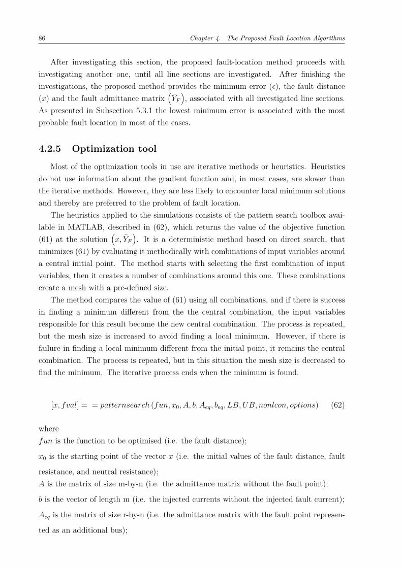
86 Chapter 4. The Proposed Fault Location Algorithms
After investigating this section, the proposed fault-location method proceeds withinvestigating another one, until all line sections are investigated. After finishing theinvestigations, the proposed method provides the minimum error (𝜖), the fault distance(𝑥) and the fault admittance matrix
(𝑌𝐹
), associated with all investigated line sections.
As presented in Subsection 5.3.1 the lowest minimum error is associated with the mostprobable fault location in most of the cases.
4.2.5 Optimization tool
Most of the optimization tools in use are iterative methods or heuristics. Heuristicsdo not use information about the gradient function and, in most cases, are slower thanthe iterative methods. However, they are less likely to encounter local minimum solutionsand thereby are preferred to the problem of fault location.
The heuristics applied to the simulations consists of the pattern search toolbox avai-lable in MATLAB, described in (62), which returns the value of the objective function(61) at the solution
(𝑥, 𝑌𝐹
). It is a deterministic method based on direct search, that
minimizes (61) by evaluating it methodically with combinations of input variables arounda central initial point. The method starts with selecting the first combination of inputvariables, then it creates a number of combinations around this one. These combinationscreate a mesh with a pre-defined size.
The method compares the value of (61) using all combinations, and if there is successin finding a minimum different from the the central combination, the input variablesresponsible for this result become the new central combination. The process is repeated,but the mesh size is increased to avoid finding a local minimum. However, if there isfailure in finding a local minimum different from the initial point, it remains the centralcombination. The process is repeated, but in this situation the mesh size is decreased tofind the minimum. The iterative process ends when the minimum is found.
[𝑥, 𝑓𝑣𝑎𝑙] = = 𝑝𝑎𝑡𝑡𝑒𝑟𝑛𝑠𝑒𝑎𝑟𝑐ℎ (𝑓𝑢𝑛, 𝑥0, 𝐴, 𝑏, 𝐴𝑒𝑞, 𝑏𝑒𝑞, 𝐿𝐵, 𝑈𝐵, 𝑛𝑜𝑛𝑙𝑐𝑜𝑛, 𝑜𝑝𝑡𝑖𝑜𝑛𝑠) (62)
where𝑓𝑢𝑛 is the function to be optimised (i.e. the fault distance);
𝑥0 is the starting point of the vector 𝑥 (i.e. the initial values of the fault distance, fault
resistance, and neutral resistance);𝐴 is the matrix of size m-by-n (i.e. the admittance matrix without the fault point);
𝑏 is the vector of length m (i.e. the injected currents without the injected fault current);
𝐴𝑒𝑞 is the matrix of size r-by-n (i.e. the admittance matrix with the fault point represen-
ted as an additional bus);

4.3. Proposed fault location algorithm 2 87
𝑏𝑒𝑞 is the vector of length r (i.e. the injected currents with the injected fault current at
the fault point);𝐴𝑒𝑞 · 𝑥 = 𝑏𝑒𝑞 represents the linear equality constraints;
𝐿𝐵 = [𝑑𝑖𝑠𝑡_𝑚𝑖𝑛𝑟𝑓_𝑚𝑖𝑛𝑟𝑛_𝑚𝑖𝑛] is the lower bound for 𝑥;
𝑈𝐵 = [𝑐𝑜𝑚𝑝𝑟𝑖𝑚𝑒𝑛𝑡𝑜− 𝑑𝑖𝑠𝑡_𝑚𝑖𝑛𝑟𝑓_𝑚𝑎𝑥𝑟𝑛_𝑚𝑎𝑥] is the upper bound for 𝑥;
𝑜𝑝𝑡𝑖𝑜𝑛𝑠 is the options structure created with 𝑝𝑠𝑜𝑝𝑡𝑖𝑚𝑠𝑒𝑡, which includes the initial mesh
size, time limit, and maximum number of iterations.
The lower bound 𝐿𝐵 and upper bound 𝑈𝐵 parameters of the optimization processare: 𝑑𝑖𝑠𝑡_𝑚𝑖𝑛 = 1.00𝑚: minimum distance value; 𝑟𝑓_𝑚𝑖𝑛 = 1.0Ω: minimum fault
resistance value; 𝑟𝑛_𝑚𝑖𝑛 = 1.0Ω: minimum neutral resistance value; 𝑐𝑜𝑚𝑝𝑟𝑖𝑚𝑒𝑛𝑡𝑜 −
𝑑𝑖𝑠𝑡_𝑚𝑖𝑛: maximum distance value; 𝑟𝑓_𝑚𝑎𝑥 = 500.0Ω: maximum fault resistance value;
𝑟𝑛_𝑚𝑎𝑥 = 500.0Ω: maximum neutral resistance value;
4.3 Proposed fault location algorithm 2
The new proposed fault location method referred to Figure 21 is based on voltagesand currents measurements. It requests information about the post-fault voltage andcurrent phasor quantities at the substation and DG buses, provided by IEDs, as well asthe distribution network operating status and electrical parameters, stored in the utility’sdatabase.
Figure 22 presents the block diagram of the proposed fault location method. Asillustrated, the algorithm starts calculating the equivalent sources at the substation busand at the buses where the DGs are connected. Then, the algorithm selects the linesection to be investigated and determines the equivalent circuit of that particular linesection. After this step it is possible to calculate the fault current, using informationabout the fault point and the fault resistance, and the post-fault voltages and currentsphasor quantities at the substation. The optimization tool is used to provide the faultdistance and fault resistances that minimizes the error between the measured and thecalculated phasor quantities at the substation.
This proposed method locates the fault point by computing the equivalent two-portnetwork representation of the line section under investigation accordingly to Subsec-tion 4.3.1, then calculating the fault current in agreement with Subsection 4.3.2.1 orSubsection 4.3.2.2 and finally comparing the measured and calculated current phasors todetermine the error.
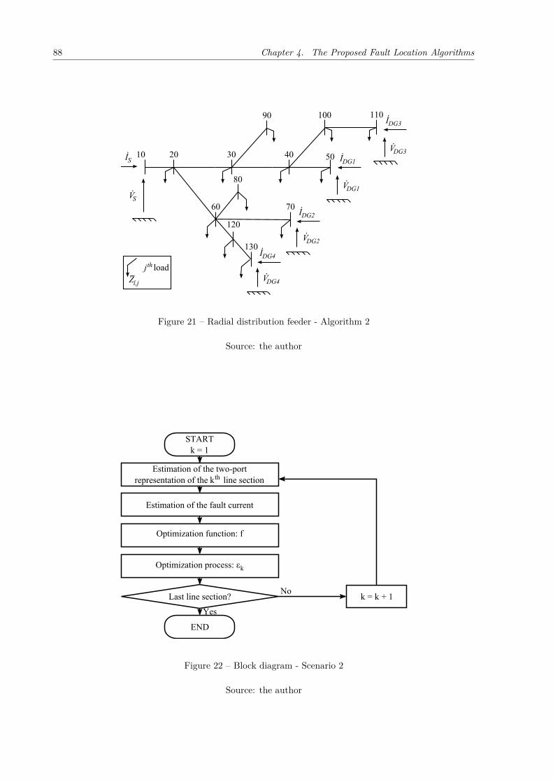
88 Chapter 4. The Proposed Fault Location Algorithms
10 3020 40 50
90
60 70
80
100 110
120
130
loadjth
l,j
IS.
VS.
IDG4.
IDG1.
VDG1.
VDG3.
VDG2.
IDG3.
IDG2.
Z VDG4.
Figure 21 – Radial distribution feeder - Algorithm 2
Source: the author
EstimationNofNtheNfaultNcurrentN
OptimizationNfunction:Nf
STARTkN=N1
OptimizationNprocess:Nεk
kN=NkN+N1LastNlineNsection?
Yes
No
END
EstimationNofNtheNtwo-portNkNNNNlineNsectionthrepresentationNofNtheN
Figure 22 – Block diagram - Scenario 2
Source: the author

4.3. Proposed fault location algorithm 2 89
4.3.1 Two-port network representation
The algorithm uses synchronized voltage and current phasor quantities recorded atthe DGs and substation buses. Then, the proposed algorithm calculates the equivalentcircuit of a given line section by means of the two-port network representation, consideringthe distributed-parameter line model, since it is more precise. The representation of atransmission line whose line length is 𝑙 is by means of the transmission matrix, consideringthe equivalent parameters at both line end (i.e. at the sending and receiving ends, denotedby the subscripts S and R, respectively), as in (63)
⎡⎣ [��𝑆
][𝐼𝑆
] ⎤⎦ = [𝑇 (𝑙)] ×
⎡⎣ [��𝑅
][𝐼𝑅
] ⎤⎦ (63)
with
[𝑇 (𝑙)] =⎡⎣ [𝐴 (𝑙)] [𝐵 (𝑙)]
[𝐶 (𝑙)] [𝐷 (𝑙)]
⎤⎦ (64)
[𝐴 (𝑙)], [𝐵 (𝑙)], [𝐶 (𝑙)], [𝐷 (𝑙)] are the transmission line matrix parameters in the two-portrepresentation, given by (65)-(68) in accordance to the procedure presented in (BOWMAN;
MCNAMEE, 1964), valid for untransposed transmission lines
[𝐴 (𝑙)] ={
[𝑈 ] + 12 × [𝑍𝜋] × [𝑌𝜋]
}(65)
[𝐵 (𝑙)] = [𝑍𝜋] (66)
[𝐶 (𝑙)] = [𝑌𝜋] ×{
[𝑈 ] + 14 × [𝑍𝜋] × [𝑌𝜋]
}(67)
[𝐷 (𝑙)] ={
[𝑈 ] + 12 × [𝑍𝜋] × [𝑌𝜋]
}(68)
where
[𝐴 (𝑙)] is the open-circuit voltage rate;
[𝐵 (𝑙)] is the negative short-circuit transfer impedance;
[𝐶 (𝑙)] is the open-circuit transfer admittance;
[𝐷 (𝑙)] is the negative short-circuit current ratio;
[𝑈 ] is the identity matrix;
[𝑍𝜋] is the line impedance of the equivalent 𝜋 line section; and
[𝑌𝜋] is the line admittance of the equivalent 𝜋 line section.

90 Chapter 4. The Proposed Fault Location Algorithms
V30.
I30.[ ]
[ ] YF
IF-30.
IF-90.
VF.
I90.
V90.
Y90,load
[ ] [ ]
[ ] [ ]T(x)[ ] [ ]
[ ]
[ ] [ ]30-90T(l -x)
Yeq x,YF( )
Y'eq
Figure 23 – Equivalent admittance in the two-port network model with source at one end
The impedance and length of distinct lateral branches may produce the same voltagesand currents at the substation bus and lead to multiple solutions, as the fault distanceand resistance are unknown. The algorithm tackles this trouble by investigating all linesections so as to determine the possible fault positions, relying on an optimization methodto minimize the errors between the phasor measurements and calculations and sort themost-likely solutions.
Considering the network depicted in Figure 21, the fault may be located along linesections that are quite different. One that is connected to an equivalent source at oneend (e.g. line section 30 − 90) and other that is connected to two equivalent sources atboth ends (e.g. line section 30 − 40). The presence or absence of sources at the bothline ends of the investigated line section may request two procedures, as explained inSubsection 4.3.2.1 and Subsection 4.3.2.2.
4.3.2 Procedures
4.3.2.1 Procedure I
The line section 30-90 illustrated in Figure 21 is used to exemplify the procedureproposed within this section. In this line section, represented by Figure 23, it can benoticed that there are voltages and currents measurements available at only one line end.
The fault point is given by solving (69), taking into consideration the voltages andcurrents phasor quantities measured at the sending end (bus 30) and the equivalent ad-mittance seen at this bus, as in the equivalent two-port network representation of thisline section, depicted in Figure 23.
⎡⎣ [��𝐹
][𝐼𝐹−90
] ⎤⎦ =⎡⎣ [𝐴 (𝑙30−90 − 𝑥)] [𝐵 (𝑙30−90 − 𝑥)]
[𝐶 (𝑙30−90 − 𝑥)] [𝐷 (𝑙30−90 − 𝑥)]
⎤⎦ ×
⎡⎣ [��90
][𝐼90
] ⎤⎦ (69)
where
𝑥 is the distance from the sending end to the fault point;
𝑙30−90 is the total length of the investigated line section;

4.3. Proposed fault location algorithm 2 91
The fault point 𝑥 and the fault admittance[𝑌𝐹
]are unknown and have to be estimated
in an iterative process, whereas the voltages and currents phasor quantities at the sendingand receiving ends are known.
The current at the receiving end is given by the equivalent admittance[𝑌90,𝑙𝑜𝑎𝑑
]mul-
tiplied by the voltage, as deduced in (70).
[𝐼90
]=
[𝑌90,𝑙𝑜𝑎𝑑
]×
[��90
](70)
Consequently,
[𝐼𝐹−90
]=
{[𝐶 (𝑙30−90 − 𝑥)] + [𝐷 (𝑙30−90 − 𝑥)] ×
[𝑌90,𝑙𝑜𝑎𝑑
]}×
[��90
](71)
and
[��𝐹
]=
{[𝐴 (𝑙30−90 − 𝑥)] + [𝐵 (𝑙30−90 − 𝑥)] ×
[𝑌90,𝑙𝑜𝑎𝑑
]}×
[��90
](72)
Hence, the fault current seen from the receiving end can be found by substituting (69)in (70), as follows:
[𝐼𝐹−90
]=
{[𝐶 (𝑙30−90 − 𝑥)] + [𝐷 (𝑙30−90 − 𝑥)] ×
[𝑌90,𝑙𝑜𝑎𝑑
]}×
×{[𝐴 (𝑙30−90 − 𝑥)] + [𝐵 (𝑙30−90 − 𝑥)] ×
[𝑌90,𝑙𝑜𝑎𝑑
]}−1×
[��𝐹
] (73)
(73) can be written as (74)
[𝐼𝐹−90
]=
[𝑌 ′𝑒𝑞
]×
[��𝐹
](74)
where
[𝑌 ′𝑒𝑞
]=
{[𝐶 (𝑙30−90 − 𝑥)] + [𝐷 (𝑙30−90 − 𝑥)] ×
[𝑌𝐹
]}×
×{[𝐴 (𝑙30−90 − 𝑥)] + [𝐵 (𝑙30−90 − 𝑥)] ×
[𝑌𝐹
]}−1 (75)
In turn, the fault current seen from the sending end can be found by substituting[𝑌 ′𝑒𝑞
]in (69), as follows:
[𝐼𝐹−30
]=
[��𝐹
]×
{[𝑌𝐹
]+
[𝑌 ′𝑒𝑞
]}(76)
Therefore:
⎡⎣ [��30
][𝐼30
] ⎤⎦ =⎡⎣ [𝐴(𝑥)] [𝐵(𝑥)]
[𝐶(𝑥)] [𝐷(𝑥)]
⎤⎦ ×
⎡⎣ [��𝐹
][𝐼𝐹−30
] ⎤⎦ (77)
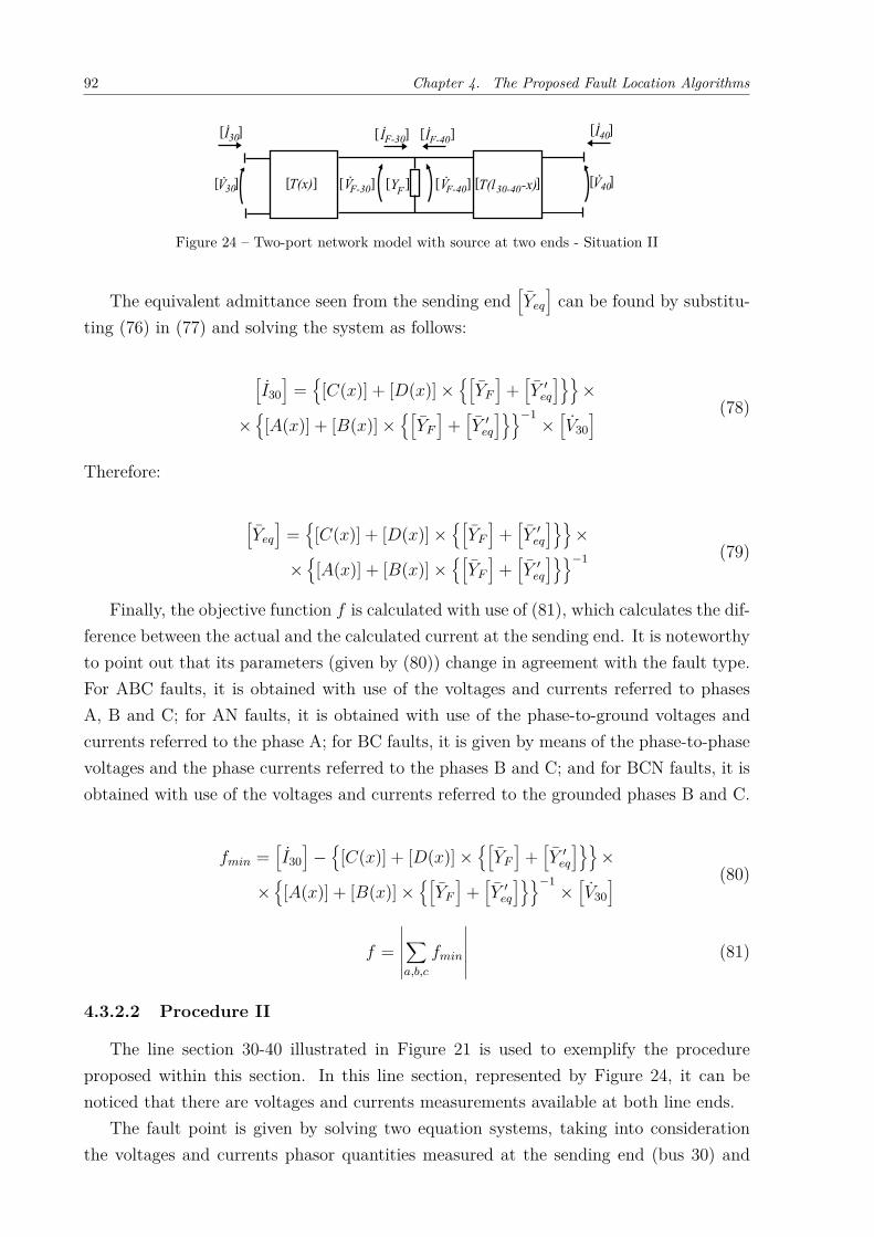
92 Chapter 4. The Proposed Fault Location Algorithms
V30.
I30.[ ]
[ ] YF
IF-30.
IF-40.
V.
[ ] [ ]
[ ] [ ]T(x)[ ] [ ]30-40T(l -x) V40
.
I40.[ ]
[ ]F-40V
.[ ]F-30
Figure 24 – Two-port network model with source at two ends - Situation II
The equivalent admittance seen from the sending end[𝑌𝑒𝑞
]can be found by substitu-
ting (76) in (77) and solving the system as follows:
[𝐼30
]=
{[𝐶(𝑥)] + [𝐷(𝑥)] ×
{[𝑌𝐹
]+
[𝑌 ′𝑒𝑞
]}}×
×{[𝐴(𝑥)] + [𝐵(𝑥)] ×
{[𝑌𝐹
]+
[𝑌 ′𝑒𝑞
]}}−1×
[��30
] (78)
Therefore:
[𝑌𝑒𝑞
]=
{[𝐶(𝑥)] + [𝐷(𝑥)] ×
{[𝑌𝐹
]+
[𝑌 ′𝑒𝑞
]}}×
×{[𝐴(𝑥)] + [𝐵(𝑥)] ×
{[𝑌𝐹
]+
[𝑌 ′𝑒𝑞
]}}−1 (79)
Finally, the objective function 𝑓 is calculated with use of (81), which calculates the dif-ference between the actual and the calculated current at the sending end. It is noteworthyto point out that its parameters (given by (80)) change in agreement with the fault type.For ABC faults, it is obtained with use of the voltages and currents referred to phasesA, B and C; for AN faults, it is obtained with use of the phase-to-ground voltages andcurrents referred to the phase A; for BC faults, it is given by means of the phase-to-phasevoltages and the phase currents referred to the phases B and C; and for BCN faults, it isobtained with use of the voltages and currents referred to the grounded phases B and C.
𝑓𝑚𝑖𝑛 =[𝐼30
]−
{[𝐶(𝑥)] + [𝐷(𝑥)] ×
{[𝑌𝐹
]+
[𝑌 ′𝑒𝑞
]}}×
×{[𝐴(𝑥)] + [𝐵(𝑥)] ×
{[𝑌𝐹
]+
[𝑌 ′𝑒𝑞
]}}−1×
[��30
] (80)
𝑓 =
∑𝑎,𝑏,𝑐
𝑓𝑚𝑖𝑛
(81)
4.3.2.2 Procedure II
The line section 30-40 illustrated in Figure 21 is used to exemplify the procedureproposed within this section. In this line section, represented by Figure 24, it can benoticed that there are voltages and currents measurements available at both line ends.
The fault point is given by solving two equation systems, taking into considerationthe voltages and currents phasor quantities measured at the sending end (bus 30) and

4.3. Proposed fault location algorithm 2 93
the receiving end (bus 40) of the network depicted in Figure 21, and the equivalent two-port network representation of this line section, depicted in Figure 24. According to thisrepresentation it is possible to write equations (82) and (83):
⎡⎣ [��𝐹−30
][𝐼𝐹−30
] ⎤⎦ =⎡⎣ [𝐴(𝑥)] − [𝐵(𝑥)]
− [𝐶(𝑥)] [𝐷(𝑥)]
⎤⎦ ×
⎡⎣ [��30
][𝐼30
] ⎤⎦ (82)
⎡⎣ [��𝐹−40
][𝐼𝐹−40
] ⎤⎦ =⎡⎣ [𝐴 (𝑙30−40 − 𝑥)] − [𝐵 (𝑙30−40 − 𝑥)]
− [𝐶 (𝑙30−40 − 𝑥)] [𝐷 (𝑙30−40 − 𝑥)]
⎤⎦ ×
⎡⎣ [��40
][𝐼40
] ⎤⎦ (83)
The fault current at a given point is given by the fault admittance multiplied by thefault voltage, as deduced in (84).
[𝑌𝐹
]×
[��𝐹
]=
[𝐼𝐹−40
]+
[𝐼𝐹−30
](84)
Therefore, the objective function 𝑓 is given by (85). It is noteworthy to point outthat its parameters change in agreement with the fault type, analogously to the function(81) described in Subsection 4.3.2.1. For ABC faults, it is obtained with use of thepositive-sequance voltages and currents; for AN faults, it is obtained with use of thephase-to-ground voltages and currents referred to the phase A; for BC faults, it is givenby means of the phase-to-phase voltages and the phase currents referred to the phases Band C; and for BCN faults, it is obtained with use of the voltages and currents referredto the grounded phases B and C.
𝑓 =
∑𝑎,𝑏,𝑐
𝑓𝑚𝑖𝑛
(85)
where 𝑓𝑚𝑖𝑛 is the sum of relative variations of the currents calculated at the sendingand receiving ends and the voltage at the fault point, as follows:
Δ𝐼30 =[𝑌𝐹
]×
[��𝐹−30
]−
{[𝐼𝐹−30
]+
[𝐼𝐹−40
]}(86)
Δ𝐼40 =[𝑌𝐹
]×
[��𝐹−40
]−
{[𝐼𝐹−30
]+
[𝐼𝐹−40
]}(87)
Δ��𝐹 =[��𝐹−30
]−
[��𝐹−40
](88)
𝑓𝑚𝑖𝑛 =
Δ𝐼40
𝑚𝑎𝑥
{Δ𝐼40
} +
Δ𝐼30
𝑚𝑎𝑥
{Δ𝐼30
} +
Δ��𝐹
𝑚𝑎𝑥
{Δ��𝐹
} (89)

94 Chapter 4. The Proposed Fault Location Algorithms
4.3.3 Comparison between measured and calculated current pha-sors
The erros between measurements and calculations at the hypothetical point of faultare obtained through the objective function 𝑓 defined for each algorithm and fault type.The investigation finishes when the optimization process provides the fault distance andthe fault admittances that minimize the objective function.
Afterwards, the proposed fault location method proceeds with another line sectionuntil all of them are investigated. After that, the minimum error (𝜖), the fault distance(𝑥) and the fault admittance matrix
(𝑌𝐹
)associated with all investigated line sections are
provided. The lowest minimum error is associated with the most probable fault locationin most cases, as shown in Subsection 5.3.2.
4.3.4 Optimization tool
Analogously to the Section 4.2, the optimization process applied to the simulationsconsists of the pattern search toolbox available in MATLAB, described in (62), whichreturns the value of the objective function 𝑓 at the solution
(𝑥, 𝑌𝐹
).
4.4 Proposed fault location algorithm 3
The proposed fault location method, also referred to Figure 16, is based on the short-circuit calculation in phase components. This technique combines features present in thefault location methods described in Section 4.2 and Section 4.3; it relies on informationabout the pre-fault and post-fault voltage and current signals recorded at the substationlevel, provided by IEDs, and the connection points of the distributed generation unitsand the operating status and electrical parameters of the distribution network, stored inthe utility’s database, whereas it locates the point of fault through the equivalent two-port network representation of the line section under investigation, calculating the faultcurrent in agreement with Subsection 4.3.2.1 or Subsection 4.3.2.2 and finally comparingthe measured and calculated voltage and current phasors at the substation to determinethe error.
The method locates the fault point by analysing all the network sections in order todetermine the fault distance and the fault resistance that produce the post-fault voltagesand currents phasor quantities measured at the substation. Since the fault distance andresistances are unknown, the proposed method relies on an optimization process thatestimates these quantities in order to minimize the error between the estimated phasorquantities and the measured ones.
Figure 25 presents the block diagram of the proposed fault location method. As illus-trated, the algorithm starts calculating the equivalent load impedances and the equivalent

4.4. Proposed fault location algorithm 3 95
EstimationOofOtheOequivalentsourcesOandOloadOimpedances
EstimationOofOtheOpost-faultOvoltagesOandOcurrentsNOphasorsOatOtheOsubstation
STARTkO=O1
OptimizationOprocess:Oεk
kO=OkO+O1LastOlineOsection?
Yes
No
END
OptimizationOfunction:Of
EstimationOofOtheOadmittanceOmatrixOkOOOinvestiagtedOlineOsectionthconsideringOtheO
Figure 25 – Block diagram - Scenario 3
Source: the author
sources at the substation bus and at the buses where the DGs are connected. Then, it as-semblies the admittance matrix of a particular line section and calculates the hypotheticalpoint of fault, inserting the estimations about the fault distance and the fault resistancein the admittance matrix. Afterwards, it calculates the post-fault voltages and currentsphasor quantities at the substation and the value of the optimization function for that linesection and uses the optimization tool to provide the fault distance and fault resistancesthat minimizes the error between the measured and the calculated phasor quantities atthe substation. This procedure is repeated until all line sections are investigated.
Therefore, the fault location method may be divided into four main steps presented inSubsection 4.4.1, Subsection 4.4.2 and Subsection 4.4.3: estimation of the equivalent sour-ces and load impedances; estimation of the equivalent two-port network representationof the investigated line section; estimation of the post-fault voltages and currents phasorquantities and comparison between the measured and calculated values at the substationbus. The optimization method is described in Subsection 4.4.4.
4.4.1 Estimation of the equivalent sources and load impedances
The algorithm proposed in this paper depends on the correct representation of loadsand generators. Hence, it assumes that impedances may represent accurately the electricloads connected to the distribution transformers, while equivalent sources and impedancesmay represent the distributed generation units and the substation, analogously to the

96 Chapter 4. The Proposed Fault Location Algorithms
Section 4.2 as presented in Subsection 4.2.1.1 and Subsection 4.2.1.2.
4.4.2 Estimation of the equivalent two-port network represen-tation of the investigated line section
The estimation of the two-port representation of the investigated line section is ana-logous to the procedure detailed in Subsection 4.3.1 considering the scenarios describedin Subsection 4.3.2.1 and Subsection 4.3.2.2 within the equivalent circuit illustrated inFigure 19. However, this fault location method includes the point of fault in the matrixrepresentation, so does the fault admittance, which means representing the fault point asan existent bus in the distribution network. In addition, the fault distance is estimatedand applied to the two-port network matrix representation so that the calculations canbe performed.
4.4.3 Estimation of the post-fault voltages and currents phasorquantities at the substation
The estimation of the post-fault voltages and currents phasor quantities at the subs-tation bus takes into consideration the equivalent two-port representation described inSubsection 4.4.2. The investigated line section is partitioned at the fault point, as in Sub-section 4.2.4, which means adding a new line and column to represent the fault point as anew bus in the admittance matrix. However, this algorithm includes the fault admittancesinstead of the fault current in the calculations, and (58) is written as (90)
[𝑌𝑏𝑢𝑠,𝐹
]=
⎡⎢⎢⎢⎢⎢⎢⎢⎢⎢⎣
. . . ... ... · · · 0· · ·
(...+ 𝑌30−𝐹
)0 · · · −𝑌30−𝐹
· · · 0(...+ 𝑌𝐹−40
)· · · −𝑌𝐹−40
· · · ... ... ... ...· · · −𝑌30−𝐹 −𝑌𝐹−40
... 𝑌𝐹 + 𝑌30−𝐹 + 𝑌𝐹−40
⎤⎥⎥⎥⎥⎥⎥⎥⎥⎥⎦(90)
Then, the algorithm determines the post-fault voltages and currents at the substationusing the modified grid nodal admittance matrix with the equivalent current sources ofthe substation and DGs, and (59) is written as (91).
⎡⎢⎢⎢⎣��10
��20...
⎤⎥⎥⎥⎦ =[𝑌𝑏𝑢𝑠,𝐹
]−1×
⎡⎢⎢⎢⎣𝐼𝑒𝑞,𝑆𝑇
...𝐼𝑒𝑞,𝐺𝐷𝑛
⎤⎥⎥⎥⎦ (91)
The post-fault current leaving the substation (bus 10) is calculated through (60).Finally, the algorithm compares the actual values to the calculated ones with use of (61).
After investigating this section, the proposed fault-location method proceeds withinvestigating another one, until all line sections are investigated. After finishing the

investigations, the proposed method provides the minimum error (𝜖), the fault distance(𝑥) and the fault admittance matrix
(𝑌𝐹
), associated with all investigated line sections.
As presented in Subsection 5.3.1 the lowest minimum error is associated with the mostprobable fault location in most of the cases.
4.4.4 Optimization tool
The optimization process applied to the simulations consists of the pattern searchtoolbox available in MATLAB, analogously to the fault location methods presented inSection 4.2 and Section 4.3, which returns the value of the objective function (61) at thesolution
(𝑥, 𝑌𝐹
).
4.5 Evaluation of the fault location algorithms
This section aims at evaluating and discussing the three algorithms presented in thischapter to tackle the problem of fault location in power distribution networks with distri-buted generation. It is important to point out that the mathematical and computationalcomplexity of the three procedures is the same. The algorithms described in Section 4.2and Section 4.4 are preferred when the Thèvenin equivalents can be estimated with useof the injected power. The former applies the fault current as an injected current inorder to compute the point of fault, whereas the latter assemblies the admittance matrixconsidering the investigated line section and including in it the estimated point of fault.In turn, the algorithm described in Section 4.3 is advantageous when the measurementsof voltages and currents are known at the substation bus and the buses where the DGsare connected.
* * *

Chapter 5Simulations and Results
5.1 General
This chapter presents the simulations and the results obtained for the scenarios takeninto account within the fault location algorithms presented in Section 4.2, Section 4.3 andSection 4.4. Then, the accuracy of the proposed fault location algorithm is evaluated infunction of the parameters applied to the simulations.
5.2 Simulation premises
The fault location system was simulated using test data produced by ATP. Short-circuit simulations were performed using a distribution feeder whose topology is depictedin Figure 16. This distribution feeder has a nominal voltage of 13.8 [kV] an is composedof a main branch, where DG1 is connected. Along the main branch there are three tappoints where lateral branches are connected and some of these branches end at DG2, DG3to DG4. The total length of the feeder is 8.7 [km], considering all line sections.
For simplification purposes, the DG units and the substation were modelled as Thè-venin equivalents or represented directly by the voltages and currents phasor quantitiesmeasured at their connection points, whereas the loads were modelled as constant impe-dances with a total consumption of 2.2 [MVA] (power factor of 0.92). These assumptionsconsider that the models applied to these elements do not interfere with the fault locationalgorithms.
The three-phase short-circuit power(𝑆3𝑓𝑠𝑐
), the line-to-ground short-circuit power(
𝑆1𝑓𝑠𝑐
)and the voltage level at the substation and DG buses are presented in Table 4,
whilst the impedances 𝑧𝑝 and 𝑧𝑚 are presented in Table 5. The poles and conductors usedin the simulation cases are typical of 13.8 [kV] voltage level and are depicted in Figure 26.The line sections were simulated using the ATP Line Constants supporting routine andthese sections are composed of 336.4 MCM ACSR phase conductors (mid-span sag of

5.2. Simulation premises 99
119.5
A B C
N
1.40.8
0.8
Obs. All distances in meters.
Figure 26 – Distribution pole
Table 4 – Short-circuit rating
Bus 𝑆3𝑓𝑠𝑐 [MVA] 𝑆1𝑓
𝑠𝑐 [MVA] �� [p.u.]Substation 1000 − 80∘ 1200 − 85∘ 1.05 0∘
DG1 100 − 85∘ 110 − 87∘ 1.00 − 2∘
DG2 80 − 75∘ 75 − 80∘ 1.01 − 1∘
DG3 100 − 87∘ 130 − 89∘ 0.99 − 3∘
DG4 70 − 80∘ 85 − 85∘ 1.03 − 1.5∘
Table 5 – Short-circuit impedance data
Bus 𝑧𝑝 [Ω] 𝑧𝑚 [Ω]Substation 0.0138 + 0.1581𝑖 0.0192 + 0.0295𝑖
DG1 0.0906 + 1.7289𝑖 0.0754 + 0.1683𝑖DG2 0.4409 + 2.5006𝑖 0.1752 + 0.2012𝑖DG3 0.0256 + 1.4647𝑖 0.0741 + 0.4371𝑖DG4 0.1953 + 2.2319𝑖 0.2772 + 0.4473𝑖
9.5 [m]) and 1/0 copper ground wires (mid-span sag of 8.5 [m]).
Table 6 presents the fault parameters applied in the ATP simulations. Four fault types,with fault resistances varying from 0 up to 50 [Ω], were simulated in 12 fault points. Asa result, 168 simulation cases were produced.

100 Chapter 5. Simulations and Results
Table 6 – Simulation data
Fault Fault Number 𝑅𝐹 Number oftype instant [ms] of points [Ω] simulations
AN 37.50 12 0, 1, 5, 6020, and 50BC 37.50 12 0, 1, 5 72BCN
ABC 37.50 12 0, 1, 5 36
5.3 Simulation results
The average error 𝜇 [𝑚], the deviation 𝜎 [𝑚], the maximum error max [𝑚], and theminimum error min [𝑚] of the proposed algorithms are presented in Subsection 5.3.1to Subsection 5.3.4, considering the first line section indicated by each fault locationprocedure. The results are based upon the assumptions displayed in Section 5.2.
Even though the indicated line section is the first ranked in most cases, it is noteworthythat the problem of fault location in distribution networks has multiple solutions. As pre-viously mentioned, the proposed methods do not aim at providing a single solution. Thus,the evaluation process takes into account not only the ideal scenario, in which all the pa-rameters are represented exactly, but also scenarios in which there are uncertainties aboutthe loads, the equivalent sources and impedances, the phasor quantities and incorrect linesections parameters, as follows.
5.3.1 Algorithm 1
In this case study, the faults were simulated at the time instant 37.5 [𝑚𝑠] in 12 pointscoincident with the buses 20-130 comprised by the distribution network illustrated inFigure 16. It is assumed in the simulations that all loads are represented correctly, thenetwork parameters are the same as simulated in ATP and equivalent sources are alsocorrect.
Table 7 indicates that the highest average error occurs for a BCN (phase-to-phase-ground fault), whereas the maximum error occurs for a ABC fault (three-phase fault) andis equal to 8.2% of the feeder’s length. The minimum errors, equal to 1 [m], are due tothe lower band parameter defined in the optimization process implemented in MATLAB.By and large, the average errors lie between 25 [m] and 110 [m] and indicate a high levelof accuracy.

5.3. Simulation results 101
Table 7 – Fault location errors for the algoritm 1
Distance error Fault typeABC AN BC BCN
𝜇 [𝑚] 101 32 26 108𝜎 [𝑚] 181 91 78 102
max [𝑚] 709 399 398 338min [𝑚] 1 1 1 1
Table 8 – Points of the applied faults
Line section Distance fromfirst bus [m] second bus [m]
10-20 1222 27820-30 362 3820-60 229 157130-40 548 5230-90 253 14760-70 98 90260-80 111 28960-120 164 13640-50 575 2540-100 482 18120-130 315 168100-110 971 29
5.3.2 Algorithm 2
In this case study, four fault types were simulated at the time instant 37.5 [𝑚𝑠] in 12fault points whose locations are given in Table 8, as follows.
The results of the proposed method for the case study without forced errors are pre-sented in Table 9. Considering the correct estimations, the maximum error occurs fora BC fault (phase-to-phase fault), equals to 5.0% of the feeder’s length, as well as thehighest average error. Except for the BC fault, the errors found in this case study arelower in comparison to the algorithm 1. The average errors lie between 4 [m] and 55 [m]and indicate a high level of accuracy.
5.3.3 Algorithm 3
In this case study, analogously to Subsection 5.3.1, the faults were simulated at thetime instant 37.5 [𝑚𝑠] in 12 points coincident with the buses 20-130 comprised by thedistribution network illustrated in Figure 16.
The results of the proposed method for the ideal scenario (without forced errors) arepresented in Table 10. Considering the correct line sections’ estimations, the maximum

102 Chapter 5. Simulations and Results
Table 9 – Fault location errors for the algorithm 2
Distance error Fault typeABC AN BC BCN
𝜇 [𝑚] 4 4 55 20𝜎 [𝑚] 8 8 125 26
max [𝑚] 36 40 438 73min [𝑚] 0 0 0 0
Table 10 – Fault location errors for the algorithm 3
Distance error Fault typeABC AN BC BCN
𝜇 [𝑚] 156 156 130 135𝜎 [𝑚] 198 224 150 155
max [𝑚] 574 916 451 617min [𝑚] 9 14 3 6
error occurs for a AN fault (phase-to-ground fault) and is equal to 10.5% of the feeder’slength, whereas the highest average errors occur for AN and ABC faults. The minimumerrors do not reach the lower band parameter defined in the optimization process imple-mented in MATLAB, since the minimum error, found for a BC fault, is equal to 3 [m].By and large, the average errors lie between 130 [m] and 160 [m] and indicate a high levelof accuracy. Nonetheless, the errors found in this case study are worse than the errorsfrom the algorithms 1 and 2, except for the maximum error calculated for a ABC fault,whose highest value is obtained in the algorithm 1.
5.3.4 Sensitivity analysis
The sensitivity analysis showed in this section aims at verifying the effect of a certainlevel of error in the estimation of equivalent sources, line parameters, loads and phasorson the proposed methods. The choice of models has taken into consideration the ease ofimplementation into the fault location algorithms.
5.3.4.1 Errors in the equivalents estimation
The proposed method estimates the equivalent sources and impedances as presentedin Section 4.2 and Section 4.4. However, the pre-fault load flow may present a certainlevel of error. Therefore, a statistical approach was used to determine the influence ofthese quantities in the fault location results. This approach consisted of multiplicatingthe equivalent sources and impedances quantities by a random number, chosen from a

5.3. Simulation results 103
Table 11 – Fault location errors with errors in the equivalent sources estimations
Distance error Fault typeABC AN BC BCN
Algorithm 1𝜇 [𝑚] 116 109 57 160𝜎 [𝑚] 198 220 126 116
max [𝑚] 849 999 398 442min [𝑚] 1 1 1 1
Algorithm 3𝜇 [𝑚] 166 176 208 182𝜎 [𝑚] 128 273 166 166
max [𝑚] 482 966 550 580min [𝑚] 32 25 25 11
normal distribution 𝒩 (𝜇, 𝜎2) with mean 𝜇 one and standard deviation 𝜎 of 10%, in orderto make them different from the ATP simulations, as in
𝐼’𝑒𝑞,𝑠𝑐 = 𝒩
(𝜇, 𝜎2
)· 𝐼𝑒𝑞,𝑠𝑐 and 𝑍’
𝑒𝑞,𝑠𝑐 = 𝒩(𝜇, 𝜎2
)· 𝑍𝑒𝑞,𝑠𝑐 (92)
where
𝒩 (𝜇, 𝜎2) is a random number;
𝑍𝑒𝑞,𝑠𝑐 is the equivalent impedance at the substation or DG; and
𝐼𝑒𝑞,𝑠𝑐 is the equivalent current source at the substation or DG.
Table 11 indicates that the maximum error referred to the algorithm 1 occurs for a ANfault (phase-to-ground fault). This error is equal to 11.5% of the feeder’s length and theaverage errors lie between 55 [m] and 160 [m]. Meanwhile, it indicates that the maximumerror related to the algorithm 3 occurs for a BCN fault and is equal to 11.49% of thefeeder’s length. The average errors lie between 60 [m] and 160 [m] and suggest a highlevel of accuracy.
5.3.4.2 Errors in the loads estimation
The proposed method estimates the loads’ impedances as presented in Section 4.2,Section 4.3 and Section 4.4. However, this approach may be innacurate since it is im-possible to determine correctly the load at each distribution transformer. Therefore, astatistical approach was used to determine the influence of these quantities in the faultlocation results, as in Subsection 5.3.4.1, with
𝐼’𝑒𝑞,𝑙𝑜𝑎𝑑 = 𝒩
(𝜇, 𝜎2
)· 𝐼𝑒𝑞,𝑙𝑜𝑎𝑑 and 𝑍’
𝑒𝑞,𝑙𝑜𝑎𝑑 = 𝒩(𝜇, 𝜎2
)· 𝑍𝑒𝑞,𝑙𝑜𝑎𝑑 (93)
where

104 Chapter 5. Simulations and Results
Table 12 – Fault location errors with errors in the load estimation
Distance error Fault typeABC AN BC BCN
Algorithm 1𝜇 [𝑚] 107 66 28 120𝜎 [𝑚] 181 167 80 121
max [𝑚] 703 860 404 406min [𝑚] 1 1 1 2
Algorithm 2𝜇 [𝑚] 5 30 8 17𝜎 [𝑚] 9 68 17 26
max [𝑚] 36 278 51 79min [𝑚] 0 0 0 0
Algorithm 3𝜇 [𝑚] 117 154 142 134𝜎 [𝑚] 114 218 162 167
max [𝑚] 362 870 524 702min [𝑚] 7 14 2 4
𝒩 (𝜇, 𝜎2) is a random number;
𝑍𝑒𝑞,𝑙𝑜𝑎𝑑 is the equivalent load impedance at a given bus; and
𝐼𝑒𝑞,𝑙𝑜𝑎𝑑 is the equivalent load current at a given bus.
Table 12 indicates that the maximum error related to the algorithm 1 occurs for a ANfault (phase-to-ground fault). This error is equal to 9.9% of the feeder’s length and theaverage errors lie between 30 [m] and 121 [m]. In addition, the maximum error referredto the algorithm 2 occurs for a AN fault (phase-to-ground fault), equals to 3.2% of thefeeder’s length. The average errors lie between 5 [m] and 30 [m] and indicate a highlevel of accuracy. Regarding the algorithm 3, the maximum error occurs for a AN fault(phase-to-ground fault), equals to 10.0% of the feeder’s length. The average errors liebetween 115 [m] and 165 [m] and indicate a high level of accuracy.
5.3.4.3 Errors in line sections parameters
The proposed method uses information about the line sections electrical parametersthat may be stored in a database. However, the actual electrical parameters may beslightly different from the stored ones. Therefore, it is necessary to evaluate the influenceof this parameters with regards to the accuracy of the proposed method. The approachused to perform this evaluation consisted of using electrical parameters different from theones simulated in ATP. The difference is related to the soil resistivity (400 [Ω ·𝑚] insteadof 100 [Ω ·𝑚]) and distribution pole geometry (phase conductors 12 [m] from the groundand neutral conductor 10 [m] from the ground). Table 13 indicates that the maximum

5.3. Simulation results 105
Table 13 – Fault location errors with errors in the line section parameters
Distance error Fault typeABC AN BC BCN
Algorithm 1𝜇 [𝑚] 72 40 90 136𝜎 [𝑚] 62 95 68 88
max [𝑚] 181 399 280 317min [𝑚] 1 1 1 8
Algorithm 2𝜇 [𝑚] 15 14 73 62𝜎 [𝑚] 12 14 98 35
max [𝑚] 54 44 289 97min [𝑚] 4 0 3 2
Algorithm 3𝜇 [𝑚] 138 149 197 177𝜎 [𝑚] 103 235 149 174
max [𝑚] 357 965 474 667min [𝑚] 9 3 33 20
error referred to the algorithm 1 occurs for a AN fault (phase-to-ground fault). This erroris equal to 4.6% of the feeder’s length and the average errors lie between 40 [m] and 140[m]. Regarding the algorithm 2, the maximum error occurs for a BC fault (phase-to-phasefault), equals to 3.3% of the feeder’s length. The average errors lie between 15 [m] and75 [m] and indicate a high level of accuracy. In turn, the maximum error referred to thealgorithm 3 occurs for a AN fault (phase-to-ground fault), equals to 11.1% of the feeder’slength. The average errors lie between 140 [m] and 200 [m] and indicate a high level ofaccuracy.
5.3.4.4 Errors in the phasors quantities
The phasor quantities may present a certain level of error because of the acquiredmeasurements. Therefore, a statistical approach was used to determine the influenceof these quantities in the fault location results by adding a random phasor error withmagnitude equals to 1% of the actual phasor quantity and angle with a random valuebetween 0 and 360 degrees, as in
𝐼’𝑒𝑞,𝑆𝐸 = 𝐼𝑒𝑞,𝑆𝐸 + Δ𝐼 (94)
where
Δ𝐼 is a random phasor error; and
𝐼𝑒𝑞,𝑆𝐸 is the equivalent current at the substation or DG bus.

106 Chapter 5. Simulations and Results
Table 14 – Fault location errors with errors in the phasor quantities
Distance error Fault typeABC AN BC BCN
Algorithm 2𝜇 [𝑚] 5 115 50 17𝜎 [𝑚] 9 359 102 24
max [𝑚] 36 1738 438 67min [𝑚] 0 0 0 0
Algorithm 3𝜇 [𝑚] 156 165 145 136𝜎 [𝑚] 122 233 165 162
max [𝑚] 362 916 551 663min [𝑚] 7 14 3 0
1 2 3 4 5 6 7 8 9 10 110
20
40
60
80
%Co
fCsi
mul
atio
nCca
ses
RankingCofCmost-likelyCsolutions
ABCANBCBCN
Figure 27 – Histogram of correct line sections identification
The results of the proposed method for this scenario are presented in Table 14. Con-sidering the correct estimations, the maximum error related to the algorithm 2 occurs fora AN fault (phase-to-ground fault), equals to 19.9% of the feeder’s length. The averageerrors lie between 5 [m] and 115 [m] and indicate a high level of accuracy. In turn, themaximum error within the algorithm 3 occurs for a AN fault (phase-to-ground fault),equals to 10.5% of the feeder’s length. The average errors lie between 136 [m] and 165[m] and indicate a high level of accuracy.
5.3.5 Histogram
Figure 27 illustrates the percentages of correct identifications of the faulted line sectionin function of the solutions ranked by the optimization process. It can be noticed thatthe correct line section is the first ranked in most cases, and that the three most-likelysolutions comprehend almost all occurrences; thereby, the first solution provided by the

fault location algorithms is highly likely to be the faulted line section, and the threefirst solutions are highly likely to indicate the faulted line section in all case studies.Nevertheless, it is noteworthy that the problem of fault location in distribution networkshas multiple solutions, as previously mentioned, and the proposed method does not aimto provide a single solution. Figure 27 presents the percentage of correct identifications,considering the case study without forced errors.
The most probable locations of the fault are ranked according to the error computedby the optimization process explained in Section 4.2 to Section 4.4. For evaluation ofthe accuracy of the proposed method, the result is assumed to be correct when the mostprobable location indicated by the algorithm matches the network section where the faultoccurred.
* * *
Conclusion
Conclusion
This report presented three fault location algorithms capable of identifying the faultedsection and locating the fault point. To do so, it was necessary to evaluate the cutting-edge fault location algorithms in power distribution networks with the presence of DGin chapter Chapter 2 and also the fault behaviour of the DG and load technologies cur-rently in use in Chapter 3. Afterwards, Chapter 4 described the proposed fault locationalgorithms, whereas Chapter 5 showed details of the simulations.
The results indicated that the proposed methods are accurate, regardless of the faulttype, but affected by errors in estimating the phasor quantities recorded at the substationand DG buses, the equivalent sources and impedances that represent the analytical modelsof the distributed generation units and the equivalent load impedances, as well as incorrectline sections parameters. Overall, the algorithm #2 presented the best results in termsof accuracy and correct line section identification, while the algorithm #3 provided theworst ones. On the whole, the results provided by the algorithm #1 are intermediatevalues between the algorithms #2 and #3, but a few exceptions were found in all casestudies.
By and large, all the proposed algorithms show that the impact of the forced errorson the fault location accuracy is relatively low, since the uncertainties did not interferewith the ability to adequately indicate the faulted line section. The average errors saw nosignificant change within a given scenario, regardless of the error added to the simulations.
Further Perspectives
Further developments and enhancements in this field of study may comprise:a) modelling: customised solutions for real-world scenarios.
b) fault location algorithm: new software tools and alternative computing methods.

109
c) fault location method: study of new procedures for fault location in power distri-bution networks with distributed generation.
d) simulations and tests: more simulations and different study cases performed withuse of different analytical models of DG units and loads developed within thisresearch project, in order to validate the proposal in different settings.
References
AKHMATOV, V. Analysis of dynamic behaviour of electric power systems withlarge amount of wind power. Tese (Doutorado) — Technical University of Denmark,2003.
ALWASH, S.; RAMACHANDARAMURTHY, V.; MITHULANANTHAN, N. Fault-location scheme for power distribution system with distributed generation. PowerDelivery, IEEE Transactions on, 2015. v. 30, n. 3, p. 1187–1195, June 2015.
APRILIA, E. C. et al. Modeling the frequency response of photovoltaic inverters. In:Innovative Smart Grid Technologies (ISGT Europe), 2012 3rd IEEE PESInternational Conference and Exhibition on. [S.l.: s.n.], 2012. p. 1–5.
BARKER, P. P.; MELLO, R. W. Determining the impact of distributed generationon power systems. i. radial distribution systems. In: Power Engineering SocietySummer Meeting, 2000. IEEE. [S.l.: s.n.], 2000. v. 3, p. 1645–1656.
BOWMAN, W.; MCNAMEE, J. Development of equivalent pi and t matrix circuitsfor long untransposed transmission lines. Power Apparatus and Systems, IEEETransactions on, 1964. v. 83, n. 6, p. 625–632, June 1964. ISSN 0018-9510.
BRAHMA, S. Fault location in power distribution system with penetration of distributedgeneration. Power Delivery, IEEE Transactions on, 2011. v. 26, n. 3, p. 1545–1553,July 2011.
BRAVO, R. et al. Load modeling transmission research. CIEE Final Project Report,2010. March 2010.
CELLI, G.; PILO, F. Optimal sectionalizing switches allocation in distribution networks.Power Delivery, IEEE Transactions on, 1999. v. 14, n. 3, p. 1167–1172, Jul 1999.
CHAPMAN, S. J. Electric Machinery Fundamentals. [S.l.]: McGraw-Hill Education,2005. (McGraw-Hill Higher Education).
110 References
CHEN, Z.; MAUN, J. C. Artificial neural network approach to single-ended fault locatorfor transmission lines. Power Systems, IEEE Transactions on, 2000. v. 15, n. 1, p.370–375, February 2000.
CONTRERAS, A.; RAMOS, G. Fault location algorithm based on shortest pathoptimization problem for distribution networks with dg. In: T D Conference andExposition, 2014 IEEE PES. [S.l.: s.n.], 2014. p. 1–5.
CUK, V. et al. Considerations on the modeling of photovoltaic systems for grid impactstudies. In: Integration of Solar Power into Power Systems, First InternationalWorkshop on. [S.l.: s.n.], 2011. p. 35–42.
EINARSSON, B. Accuracy and Reliability in Scientific Computing. [S.l.]: Societyfor Industrial and Applied Mathematics, 2005.
FARRET, F. A.; oES, M. G. S. Integration of Alternative Sources of Energy.[S.l.]: Wiley, 2006.
FENGLING, H. et al. Distinguish real or false fault of single line-to-ground short-circuitfor radial distribution network. In: Power System Technology, 1998. Proceedings.POWERCON ’98. 1998 International Conference on. [S.l.: s.n.], 1998. v. 1, p.260–264 vol.1.
FOX, B. Wind power integration: connection and system operational aspects.[S.l.]: IET, 2007.
GERS, J. M.; HOLMES, E. J. Protection of Electricity Distribution Networks.[S.l.]: Institution of Engineering and Technology, 2011. (Energy Engineering).
GHADERI, A.; MOHAMMADPOUR, H.; GINN, H. Active fault location in distributionnetwork using time-frequency reflectometry. In: Power and Energy Conference atIllinois (PECI), 2015 IEEE. [S.l.: s.n.], 2015. p. 1–7.
GHORBANI, J.; CHOUDHRY, M. A.; FELIACHI, A. Fault location and isolation usingmulti agent systems in power distribution systems with distributed generation sources.In: Innovative Smart Grid Technologies (ISGT), 2013 IEEE PES. [S.l.: s.n.],2013. p. 1–6.
GILBERT, D. M.; MORRISON, I. F. A statistical method for the detection of powersystem faults. International Journal of Electrical Power and Energy Systems,1997. v. 19, n. 4, p. 269–275, 1997.
GIRGIS, A. A.; FALLON, C. M.; LUBKEMAN, D. L. A fault location technique forrural distribution feeders. Industry Applications, IEEE Transactions on, 1993.v. 29, n. 6, p. 1170–1175, November 1993.
GONZÁLEZ-LONGATT, F.; WALL, P.; TERZIJA, V. Wake effect in wind farmperformance: Steady-state and dynamic behavior. Renewable Energy, 2012. v. 39,n. 1, p. 329 – 338, 2012.
GUO-FANG, Z.; YU-PING, L. Development of fault location algorithm for distributionnetworks with dg. In: Sustainable Energy Technologies, 2008. ICSET 2008.IEEE International Conference on. [S.l.: s.n.], 2008. p. 164–168.

References 111
HAGH, M. T.; HOSSEINI, M. M.; ASGARIFAR, S. A novel phase to phase faultlocation algorithm for distribution network with distributed generation. In: Integrationof Renewables into the Distribution Grid, CIRED 2012 Workshop. [S.l.: s.n.],2012. p. 1–4.
HANNINEN, S.; LEHTONEN, M. Characteristics of earth faults in electrical distributionnetworks with high impedance earthing. Electric Power Systems Research, 1998.v. 44, n. 3, p. 155 – 161, 1998.
HE, L. et al. Enhanced distribution feeder fault location. In: Protective RelayEngineers, 2014 67th Annual Conference for. [S.l.: s.n.], 2014. p. 250–263.
IEEE-C37.114-WG. IEEE Guide for Determining Fault Location on ACTransmission and Distribution Lines. [S.l.], 2015. 1-76 p.
IEEE-STD.1234-2007. IEEE Guide for Fault Locating Techniques on ShieldedPower Cable Systems. [S.l.], 2007. 1-37 p.
IOV, F. et al. Mapping of grid faults and grid codes. [S.l.]: Risø NationalLaboratory, 2007.
JAGADURI, R. T.; RADMAN, G. Modeling and control of distributed generationsystems including PEM fuel cell and gas turbine. Electric Power Systems Research,2007. v. 77, n. 1, p. 83 – 92, 2007.
JANSSEN, P.; SEZI, T.; MAUN, J.-C. Optimal fault location in distribution systemsusing distributed disturbance recordings. In: Innovative Smart Grid Technologies(ISGT Europe), 2011 2nd IEEE PES International Conference and Exhibitionon. [S.l.: s.n.], 2011. p. 1–7.
JARDINI, J. et al. Daily load profiles for residential, commercial and industrial lowvoltage consumers. Power Delivery, IEEE Transactions on, 2000. v. 15, n. 1, p.375–380, Jan 2000.
JAUCH, C. et al. Simulation of the impact of wind power on the transient fault behaviorof the Nordic power system. Electric Power Systems Research, 2007. v. 77, n. 2, p.135 – 144, 2007.
JOHNSON, B. W. Out of Sight, Out of Mind? [S.l.]: Edison Electric Institute, 2006.
KANELLOS, F. D.; KABOURIS, J. Wind farms modeling for short-circuit levelcalculations in large power systems. Power Delivery, IEEE Transactions on, 2009.v. 24, n. 3, p. 1687–1695, July 2009.
KORBICZ, J. Fault Diagnosis: Models, Artificial Intelligence, Applications.[S.l.]: Springer-Verlag Berlin Heidelberg, 2004. (Engineering online library).
KOSTEREV, D.; MEKLIN, A. Load modeling in wecc. In: Power SystemsConference and Exposition, 2006. PSCE ’06. 2006 IEEE PES. [S.l.: s.n.], 2006.p. 576–581.
KUNDUR, P.; BALU, N. J.; LAUBY, M. G. Power system stability and control.[S.l.]: McGraw-Hill New York, 1994.

112 References
LESIEUTRE, B. Load Modeling Transmission Research: Final Project Report.[S.l.: s.n.], 2008. (Final project report / Energy Research and Development Division).
LINDGREN, L.; SVENSSON, J.; GERTMAR, L. Generic models for wind powerplants-needs and previous work. Elforsk technical report, 2012. 2012.
MAJIDI, M.; ARABALI, A.; ETEZADI-AMOLI, M. Fault location in distributionnetworks by compressive sensing. Power Delivery, IEEE Transactions on, 2015.v. 30, n. 4, p. 1761–1769, Aug 2015. ISSN 0885-8977.
MANASSERO, G. J. et al. Fault-location system for multiterminal transmission lines.Power Delivery, IEEE Transactions on, 2010. IEEE, v. 25, n. 3, p. 1418–1426, 2010.
MANASSERO, G. J.; TAKEDA, V.; FREITAS, P. R. R. de. Algoritmo para localizaçãode faltas em redes de distribuição de energia elétrica com a presença de unidades degeração distribuída. In: Electricity Distribution (CIDEL), 2014 InternationalConference on. [S.l.: s.n.], 2014. p. 1–6.
MARTINEZ, J. et al. Short circuit signatures from different wind turbine generator types.In: Power Systems Conference and Exposition (PSCE), 2011 IEEE/PES. [S.l.:s.n.], 2011. p. 1–7.
MARTINS, M. et al. Validation of fixed speed wind turbine dynamic models withmeasured data. Renewable Energy, 2007. v. 32, n. 8, p. 1301 – 1316, 2007.
MARUSIC, A.; GRUHONJIC-FERHATBEGOVIC, S. A computerized fault locationprocess for overhead radial distribution feeders. In: Electrotechnical Conference,2006. MELECON 2006. IEEE Mediterranean. [S.l.: s.n.], 2006. p. 1114–1117.
MILANOVIC, J. V. et al. International industry practice on power system load modeling.Power Systems, IEEE Transactions on, 2013. v. 28, n. 3, p. 3038–3046, August2013.
MORA-FLOREZ, J.; MORALES-ESPANA, G.; PEREZ-LONDONO, S. Learning-basedstrategy for reducing the multiple estimation problem of fault zone location in radialpower systems. Generation, Transmission Distribution, IET, 2009. v. 3, n. 4, p.346–356, April 2009.
MORREN, J.; HAAN, S. W. H. de. Short-circuit current of wind turbines with doublyfed induction generator. Energy Conversion, IEEE Transactions on, 2007. v. 22,n. 1, p. 174–180, March 2007.
NUNES, J. U. N. de; BRETAS, A. S. An extended fault location formulation forunbalanced distribution feeders with distributed generation. In: Modern ElectricPower Systems (MEPS), 2010 Proceedings of the International Symposium.[S.l.: s.n.], 2010. p. 1–6.
OROZCO-HENAO, C.; MORA-FLOREZ, J.; PEREZ-LONDONO, S. A robustmethod for single phase fault location considering distributed generation and currentcompensation. In: Transmission and Distribution: Latin America Conferenceand Exposition (T&D-LA), 2012 Sixth IEEE/PES. [S.l.: s.n.], 2012. p. 1–7.
PETRU, T.; THIRINGER, T. Modeling of wind turbines for power system studies.Power Engineering Review, IEEE, 2002. v. 22, n. 9, p. 58–58, September 2002.
References 113
PURUSHOTHAMA, G. K. et al. ANN applications in fault locators. InternationalJournal of Electrical Power and Energy Systems, 2001. v. 23, n. 6, p. 491 – 506,2001.
RAJEEV, A.; ANGEL, T.; KHAN, F. Fault location in distribution feeders withoptimally placed pmu’s. In: Advancements in Power and Energy (TAP Energy),2015 International Conference on. [S.l.: s.n.], 2015. p. 438–442.
SAHA, M. M.; IZYKOWSKI, J.; ROSOLOWSKI, E. Fault Location on PowerNetworks. [S.l.]: Springer London, 2010. (Power Systems).
SAHA, M. M.; PROVOOST, F.; ROSOLOWSKI, E. Fault location method for mvcable network. In: Developments in Power System Protection, 2001, SeventhInternational Conference on (IEE). [S.l.: s.n.], 2001. p. 323–326.
SALIM, R. H. et al. Extended fault-location formulation for power distribution systems.Power Delivery, IEEE Transactions on, 2009. v. 24, n. 2, p. 508–516, April 2009.
SENGER, E. C. et al. Automated fault location system for primary distributionnetworks. Power Delivery, IEEE Transactions on, 2005. IEEE, v. 20, n. 2, p.1332–1340, 2005.
SHORT-CIRCUIT currents in three-phase a.c. systems - Part 0: Calculation of currents.IEC 60909.0-2001, 2001. p. 1–144, July 2001.
SPERANDIO, M. et al. Fault location in distribution networks by combining studiesof the network and remote monitoring of protection devices. In: Universities’ PowerEngineering Conference (UPEC), Proceedings of 2011 46th International.[S.l.: s.n.], 2011. p. 1–6.
SRINIVASAN, K.; ST.-JACQUES, A. A new fault location algorithm for radialtransmission lines with loads. Power Delivery, IEEE Transactions on, 1989. v. 4,n. 3, p. 1676–1682, July 1989.
SULLA, F. Fault behavior of wind turbines. Tese (Doutorado) — Lund University,2012.
SWEETING, D. Applying iec 60909, short-circuit current calculations. In: Petroleumand Chemical Industry Conference (PCIC), 2011 Record of ConferencePapers Industry Applications Society 58th Annual IEEE. [S.l.: s.n.], 2011.p. 1–6.
TANG, Y. et al. Fault indicators in transmission and distribution systems. In: ElectricUtility Deregulation and Restructuring and Power Technologies, 2000.Proceedings. DRPT 2000. International Conference on. [S.l.: s.n.], 2000. p.238–243.
TAWFIK, M. M.; MORCOS, M. M. ANN-based techniques for estimating fault locationon transmission lines using prony method. Power Delivery, IEEE Transactions on,2001. v. 16, n. 2, p. 219–224, April 2001.
TEODORESCU, R.; LISERRE, M.; RODRÍGUEZ, P. Grid Converters forPhotovoltaic and Wind Power Systems. [S.l.]: Wiley, 2010. (Wiley - IEEE).
114 References
THIRINGER, T.; PETERSSON, A.; PETRU, T. Grid disturbance response of windturbines equipped with induction generator and doubly-fed induction generator. In:Power Engineering Society General Meeting, 2003, IEEE. [S.l.: s.n.], 2003. v. 3,p. 1542–1547.
THUKARAM, D.; KHINCHA, H.; VIJAYNARASIMHA, H. Artificial neural networkand support vector machine approach for locating faults in radial distribution systems.Power Delivery, IEEE Transactions on, 2005. v. 20, n. 2, p. 710–721, April 2005.ISSN 0885-8977.
VITTAL, V.; AYYANAR, R. Grid Integration and Dynamic Impact of WindEnergy. [S.l.]: Springer Science & Business Media, 2012.
WANG, C. Modeling and control of hybrid wind photovoltaic fuel celldistributed generation systems. Tese (Doutorado) — Montana State University,2006.
WECC-MVWG. Composite load model for dynamic simulations. WECC MVWGLoad Model Report ver.1.0, 2012. June 2012.
WU, L.-P. et al. A new adaptive matrix algorithm for fault location in distributionnetwork with distributed generation. In: Electrical and Control Engineering(ICECE), 2011 International Conference on. [S.l.: s.n.], 2011. p. 499–504.
WU, N. A new fault location algorithm for distribution network with dg. In: ElectricityDistribution (CICED), 2010 China International Conference on. [S.l.: s.n.],2010. p. 1–7.
ZAVALIS, T. G.; BEHM, M.; LINDBERGH, G. Investigation of short-circuit scenariosin a lithium-ion battery cell. Journal of the Electrochemical Society, 2012. v. 159,n. 6, p. 848–859U, 2012.
ZHIHAI, T. et al. An accurate fault location method of smart distribution network. In:Electricity Distribution (CICED), 2014 China International Conference on.[S.l.: s.n.], 2014. p. 916–920.
ZHU, J.; LUBKEMAN, D.; GIRGIS, A. Automated fault location and diagnosis onelectric power distribution feeders. Power Delivery, IEEE Transactions on, 1997.v. 12, n. 2, p. 801–809, Apr 1997.