Fringe Benefits and Job Satisfaction

By

Benjamin Artz

Working Paper 08 - 03

University of Wisconsin – Whitewater Department of Economics

4th Floor Carlson Hall 800 W. Main Street

Whitewater, WI 53538

Tel: (262) 472 -1361

Fringe Benefits and Job Satisfaction

Benjamin Artz

University of Wisconsin – Milwaukee

Abstract Fringe benefits stand as an important part of compensation but confirming their role in determining job satisfaction has been mixed at best. The theory suggesting this role is ambiguous. Fringe benefits represent a desirable form of compensation but might result in decreased earnings and reduced job mobility. Using a pooled cross-section of five NLSY waves, fringe benefits are established as significant positive determinants of job satisfaction, even after controlling for individual fixed effects and testing for the endogeneity of fringe benefits. JEL Classification Codes: C23, J28, J32 ______________________ Contact Address: Benjamin Artz, Department of Economics, University of Wisconsin – Milwaukee, Milwaukee, WI 53201, USA. [email: bmartz@uwm.edu]

2

1. Introduction Establishing the determinants of job satisfaction remains at the forefront of

empirical testing in using measures of on-the-job utility. At first consideration, desirable

job attributes such as fringe benefits should increase job satisfaction. However, the past

evidence is mixed at best and contradictory at worst. While a valuable form of

compensation, employer provided benefits may lower earnings or reduce job mobility.

Thus, the theoretical impact of fringe benefits on job satisfaction is not immediately

clear.

Fringe benefits can impact job satisfaction in several ways. First, fringe benefits

stand as an important component of worker compensation. The National Compensation

Survey conducted by the Bureau of Labor Statistics estimated that benefits made up 30%

of total compensation for all civilian workers in 20061. Some benefits such as Social

Security and Medicare are legally required and make up roughly 27% of all benefit

compensation. The remaining 73% of benefit compensation is comprised mostly of paid

leave, insurance plans and retirement and savings plans. These benefits are often not

subject to taxation and are therefore cheaper to gain through an employer than through

the market (Alpert, 1987). Consequently, cheaper benefits should increase worker job

satisfaction.

Second, fringe benefits can act as substitutes for wages. Baughman, DiNardi and

Holtz-Eakin (2003) examined employer survey data and found that employers decreased

wages once several benefits had been offered to employees after a few years. Woodbury

(1983) found that workers also view benefits and wages as substitutes, willing to give up

wages in exchange for more benefits. This substitution can increase job satisfaction if the

3

worker’s marginal income tax rate increases. The less taxed fringe benefits can be

substituted for wages and increase job satisfaction by saving the worker from increased

tax burden.

Third, the substitution between wages and benefits can have a negative impact on

job satisfaction if workers find they must sacrifice wages and accept provision of a fringe

benefit they do not necessarily desire. For instance, workers’ spouses may already have

provision of a particular fringe benefit, so a second provision of that fringe benefit may

be viewed as wasteful and can therefore decrease job satisfaction. On the other hand,

workers may find a particular fringe benefit as essential. As a result workers may have a

feeling of job-lock to a particular employer or job if they are uncertain about the

provision of the necessary fringe benefit at a different place of work. This combination

of uncertainty and job-lock can decrease job satisfaction as well.

Since the expected impact of fringe benefits on job satisfaction is unclear, it is not

surprising that past research is inconclusive. When included in typical estimates, the

impact of fringe benefits on job satisfaction is rarely significant. In addition, the

evidence mainly depends on cross-sectional comparisons, raising questions about

potential biases. First, the impact of a particular fringe benefit on job satisfaction can be

misleading if the worker has unmeasured individual specific determinants of job

satisfaction. Indeed, we cannot assume that workers are randomly sorted into jobs but

rather that they sort themselves into the jobs that suit their preferences. In addition, job

satisfaction and fringe benefits may be simultaneously determined such that fringe

benefits are endogenous in determining job satisfaction.

4

Thus the relationship between fringe benefits and job satisfaction has not been

appropriately tested. Very little past research has isolated and examined fringe benefits

as a primary determinant of job satisfaction, few studies have included as many fringe

benefits as are available in the National Longitudinal Survey of Youth (NLSY) and none

have studied the relationship between fringe benefits and job satisfaction in detail,

controlling for fixed effects and endogeneity.2

In distinction to past results, a pooled cross-section of five NLSY waves confirms

the importance of fringe benefits in determining job satisfaction. Then, in order to test

for the simultaneous determination of fringe benefits and job satisfaction, a recursive

bivariate probit model is used to test for the possible correlation between the disturbances

in job satisfaction and fringe benefit structural equations. The cross-equation correlation

is not significantly different from zero, implying that fringe benefits can be treated as

exogenous in an estimation of job satisfaction and can be properly estimated within the

ordered probit framework used in the pooled cross-section. Finally, the role of

unobservable characteristics is controlled for by estimating fixed effects regressions.

The following section discusses the results of previous research as well as the

importance of controlling for fixed effects and testing for endogeneity in determining the

relationship between fringe benefits and job satisfaction. Section three outlines the data

and empirical methodology used to control for fixed effects and endogeneity. Section

four discusses the results, section five outlines further robustness checks and the final

section concludes.

5

2. Past Research and the Importance of Fixed Effects and Endogeneity Testing

Over the past four decades, economists have given job satisfaction increasing

attention. Job satisfaction is negatively related to job turnover (Freeman, 1978, McEvoy

and Cascio, 1985, Akerlof et al., 1988, Weiss, 1984), absenteeism (Clegg, 1983), and

positively related to productivity (Mangione and Quinn, 1975). Therefore it is useful to

understand which job characteristics and provisions increase job satisfaction.

Although fringe benefits stand as an important piece of worker compensation

packages they have not been given much attention in the job satisfaction literature.

Fringe benefits have merely acted as controls in most studies and not as the primary

subject of scrutiny. Indeed, more than one or two measures of fringe benefits are rarely

found as independent variables in job satisfaction studies.

Rather, pensions often act as the predominant proxy for fringe benefit provision

within the job satisfaction literature and consequently the estimated impact of fringe

benefits on job satisfaction. Some studies find that pensions do not significantly impact

job satisfaction in cross-section estimates. Artz (2008) uses the Working in Britain 2000

dataset and finds that pensions have no significant impact on job satisfaction. Donohue

and Heywood (2004) find a similar result in the tenth wave of the National Longitudinal

Survey (NLS) regarding employer-provided retirement plans. Others find that pensions

positively impact job satisfaction. Bender, Donohue and Heywood (2005) find this result

in the 1997 wave of the National Study of the Changing Workforce. Heywood and Wei

(2006) also find significantly positive estimates of pension’s impact on job satisfaction

using the 1988 wave of the NLS. Finally, Bender and Heywood (2006) find pensions

6

positively impact job satisfaction among Ph.D. graduates using the 1997 Survey of

Doctorate Recipients.

Still others find that pensions reduce job satisfaction. Heywood et al. (2002) use

the 1991 – 1994 waves of the British Household Panel Study finding that pensions

negatively impact job satisfaction in cross section estimates. Finally, Luchak and

Gellatly (2002) study the impact of pension accrual on job satisfaction using a dedicated

sample of 429 employees in a large, unionized public utility company in Canada. They

posit that as employees’ pensions increase in value over their job tenure, workers may

feel more vulnerable to job loss since firms may opportunistically layoff employees to

reduce pension liabilities. The authors use this hypothesis to explain their result that

pension accrual decreases job satisfaction.3

Although pensions are the predominant proxy for fringe benefits, some authors do

include multiple fringe benefit measures as independent variables in their respective

models. Donohue and Heywood (2004) report positively significant estimates for such

variables as paid vacation and sick pay but no significance for any of the remaining

benefits: child care, pension, profit sharing, employer provided training/education and

health insurance.4 Uppal (2005) uses a measure comprised of the number of fringe

benefits employees receive and finds that this is positively related to job satisfaction.

However, Benz (2005) includes most of the fringe benefits found in NLS waves 1994-

2000 in his study of employees of non-profit organizations and finds only two out of nine

fringe benefits are positive and significantly related to job satisfaction and that one is

negative and significant.

7

Another field of study examines the impact of family friendly work policies on

job satisfaction and is yet another source of research that includes multiple fringe benefit

measures5. For instance, Saltzstein et al. (2001), using the 1991 Survey of Federal

Government Employees, find disparity among the impact of family friendly work

practices on job satisfaction. Both flexible and compressed work schedules significantly

reduce job satisfaction whereas child care and the ability to work at home significantly

increase job satisfaction. However, Bryson et al. (2005), using the linked employer-

employee British Workplace Employee Relations Survey of 1998, find that the

availability of family friendly policies do not significantly increase job satisfaction.

The ambiguous results of past estimates arise primarily from the conflicting

theoretical effects that fringe benefits can have on job satisfaction, but theory may not be

the only explanation for the differences. Some of these mixed results may stem from the

use of alternative sources of data or from the institutions of different countries, primarily

the United States and Britain. Yet another source of the inconclusive results could be

dependence on potentially biased methods of estimation that fail to control for worker

fixed effects or the possible endogeneity of fringe benefits.

First, as an alternative to controlling for fixed effects using panel data, researchers

often control for a variety of selection biases in their cross-section estimates. Bender and

Heywood (2006) control for workers’ selection into the academic sector or nonacademic

sector by using instruments correlated with sector choice but not with job satisfaction.6

McCausland et al. (2005) use instruments to control for worker selection into

performance pay schemes and find that selection is only evident among workers who do

not receive performance-based pay. Bryson et al. (2005) control for worker selection into

8

unions and find that union membership does not impact worker job satisfaction.

Therefore, researchers do agree that non-random worker sorting into various workplace

characteristics is evident. Without accounting for worker sorting, the mixed cross-section

results may be unreliable. Unobservable individual preferences decide, at least in part,

the worker’s job satisfaction but also what fringe benefits workers receive. In order to

discover the true impact of fringe benefits on job satisfaction, we must first hold the

effects of unmeasured individual preferences on job satisfaction fixed and only allow

observable worker and job characteristics including the provision of fringe benefits to

vary. This is only possible by using panel data. As workers move from job to job, their

preferences are assumed to remain constant but their fringe benefits are allowed to vary.

Therefore, if worker job satisfaction changes, it is due to changes only in fringe benefits

and other measurable characteristics. In this way, fringe benefits are identified as

additional determinants of job satisfaction.

Second, a formal test of endogeneity between fringe benefits and job satisfaction

has not been undertaken. Although not with job satisfaction, fringe benefits such as

pensions, health insurance and paid vacations have been found to be endogenous in wage

regressions and thus result in simultaneity bias in ordinary least squares estimates (Jensen

and Morrisey, 2001). Since wages and job satisfaction are highly related, it is possible

that endogeneity between fringe benefits and wages could raise a similar simultaneity

bias between fringe benefits and job satisfaction. Therefore, a test for endogeneity

should be employed to be certain that a two-stage least squares estimation is not required

to control for the correlation in the error terms that jointly determine job satisfaction and

fringe benefits.

9

3. Data and Methodology

The data used are five waves of the National Longitudinal Survey of Youth with

each wave representing every other year from 1996 through 2004. All five waves of this

United States data contain a measure of overall job satisfaction and dozens of control

variables including occupation and industry codes as well as demographic and job

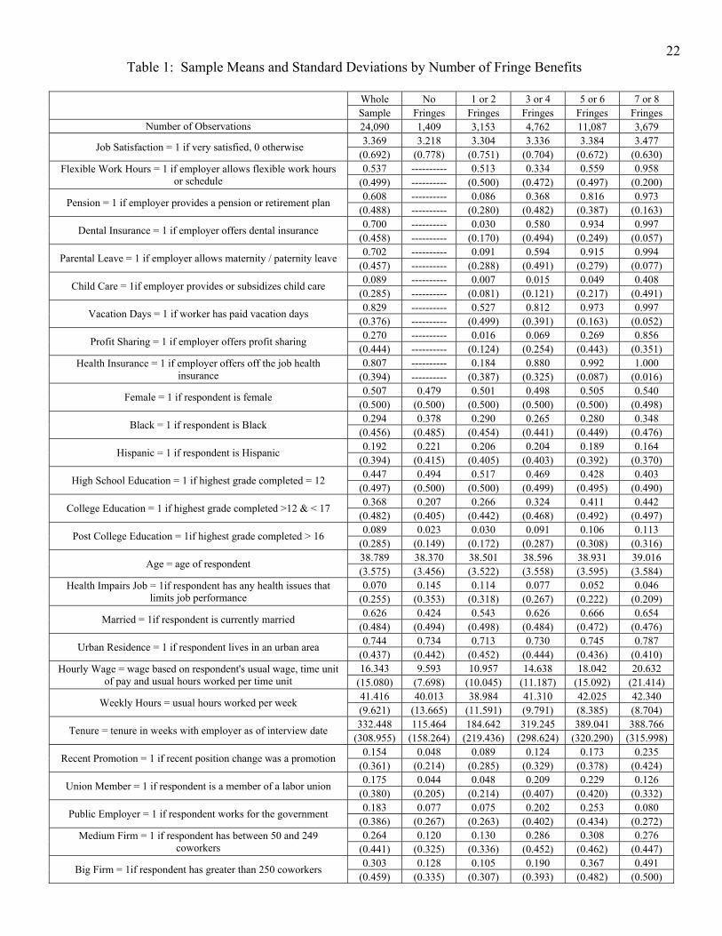
characteristics. The means, standard deviations and definitions of all utilized variables

taken from the 1996 wave are presented in Table 1 and are categorized by number of

fringe benefits workers claim to have. The NLSY is unique in that it offers many

different kinds of fringe benefit variables for analysis as well as longitudinal data that can

be used to control for fixed effects. This paper specifically includes eight different fringe

benefits as well as generated variables representing the quantity of these benefits

individuals claim to have.

The summary statistics in Table 1, grouped by quantity of benefits, support the

existence of internal labor markets within firms. In internal labor markets, payment and

correspondingly fringe benefits are tied more to the job than to the individual (Creedy

and Whitfield, 1988). Those jobs that offer the most fringe benefits are more likely to be

in big firms where internal promotion is more possible. These jobs are also more likely

to offer higher wages, implying that fringe benefits are not only tied to wages but also

may be the result of a tournament structure within firms. As a result, those workers at the

top of the tournament ladder not only have more fringe benefits and wages but may also

have a higher job satisfaction as well.

Overall job satisfaction is measured on a scale of one to four, four representing

the highest level of job satisfaction. The typical cross-section estimate of job satisfaction

10

fits this Likert scale to the cumulative normal distribution through the ordered-probit

estimation. An ordered-probit estimation is commonly used in order to capture all of the

variation between subjective measures of job satisfaction that are not necessarily linear in

nature. Although this study uses the ordered-probit technique in the individual wave and

pooled cross-section estimations, a straightforward translation to a fixed effects estimator

is provided by a dichotomous logit procedure, the conditional logit. This method

estimates whether or not a worker is very satisfied using the NLSY waves as panel data

and is based on the cumulative logistic distribution rather than the cumulative normal

distribution. The logistic and normal distributions are quite similar, thus the logit and

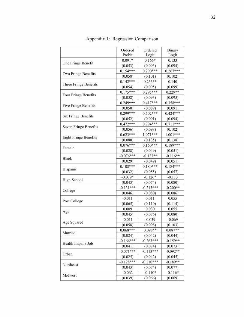
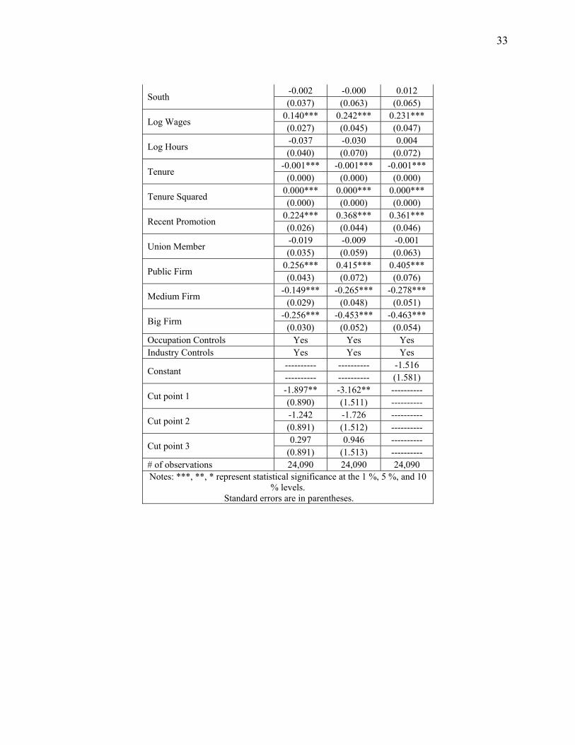
probit estimation results are comparable. These are presented in Appendix 1 and confirm

that the ordered-probit results generally carry over to the ordered-logit results and also to

the dichotomous logit results.

The conditional logit estimation technique is used to control for fixed effects

among the five NLSY waves of data. In this procedure, individual workers are first

categorized into groups by their NLSY identification number across all five waves so that

each group, or individual worker, consists of all the observations attributable to that

worker. The conditional logit then drops all of the groups that do not exhibit a change in

their job satisfaction at all across the five waves. These individuals do not contribute to

the likelihood function and therefore have no effect on the conditional probability of very

high job satisfaction. Finally, the conditional logit removes any independent variables

from the regression that do not vary at all over the five waves of data. These variables

exhibit no within-group variation across the waves and include not only race and gender

but also those preferences among workers that are unobservable and assumed to remain

11

constant. The result is a conditional probability of very high job satisfaction based

entirely on observed characteristics of workers and jobs and not on fixed effects.7 The

conditional logit model is more thoroughly presented in Appendix 2. Since cross-section

estimations cannot drop unobservable characteristics from the regressions, the estimated

impacts of fringe benefits on job satisfaction are biased.

A separate problem may arise from the inability of the individual waves of the

NLSY to exhibit enough variation among fringe benefits and job satisfaction to properly

estimate the impact of fringe benefits on job satisfaction. Therefore, pooled cross-section

estimation is used to expand the sample size. Since pooling longitudinal data generally

causes serial-correlation among independent variables, clustering standard errors by

individual respondent is necessary to maintain consistent estimators. After doing so, the

dataset contains a larger sample size and so gives more convincing results.

However, fringe benefits may still be simultaneously determined with job

satisfaction and a simple pooled cross-section does not control for this endogeneity issue.

Since job satisfaction and fringe benefits are both non-linear categorical variables, it is

difficult to employ a two-stage least squares estimation technique to control for the

possible endogeneity. Therefore a recursive bivariate probit estimation is used to test for

endogeneity between fringe benefits and job satisfaction. Consider the following

structural equations explaining job satisfaction and fringe benefits:

kk2k1k

kk2k1k

IXF

FXJS

μαα

εββ

++=

++=

where k indexes an individual worker, F is the worker’s fringe benefit provision, X is a

vector of independent variables influencing both the job satisfaction and fringe benefit

12

provision of the worker, I is an instrument that impacts fringe benefit provision but is not

significantly related to job satisfaction and ε and μ are random error terms. If fringe

benefits are indeed endogenous to job satisfaction, then the error terms in the structural

equations should be significantly correlated.

In order to proceed with the recursive bivariate probit approach, job satisfaction is

first transformed into a binary job satisfaction variable that equals one when respondents’

job satisfaction is very high and zero otherwise. A binary form of fringe benefit

provision must also be created. A dummy is therefore generated for each particular

fringe benefit as well as the minimum quantity of fringe benefits each worker claims to

have, from one benefit to eight. For instance, the dummy variable representing four

fringe benefits equals one for all individuals claiming to have at least four fringe benefits

and zero for all those with less than four. In all, sixteen generated binary forms of fringe

benefit provision are used in sixteen different recursive bivariate probit estimations.

The instrument used in the recursive bivariate probit (I) must be correlated with

fringe benefits provision, but at the same time must not impact job satisfaction. The

chosen instrument is whether or not the respondent or the respondent’s spouse has other

sources of income besides their main job. This instrument is positively related to fringe

benefits but not significant in determining job satisfaction. This might be the case

because a worker is more likely to give up wages at his primary job in exchange for

fringe benefits if there is another source of income for the worker. But that extra income

will not dictate how much a worker is satisfied with his primary job.

Estimation of the recursive bivariate probit model explained above and the

following endogeneity testing follows from Monfardini and Radice (2008). The authors

13

explain that, unless there is a very large sample, the likelihood ratio test of the cross-

equation correlation coefficient is the best test for endogeneity of the fringe benefit

dummy variable. If the correlation coefficient between the error terms ε and μ is

significantly different from zero, then the fringe benefit dummy is indeed endogenous.

This paper’s results will show the opposite. The likelihood ratio test of the correlation

coefficient rho confirms that it is not significantly different from zero, confirming that

fringe benefits can indeed be treated as exogenous in job satisfaction estimations.

Therefore the pooled cross-section results are not subject to simultaneity bias and two-

staged least squares estimation is not needed for consistent estimations.

4. Results

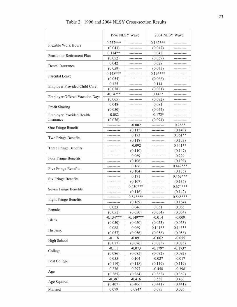
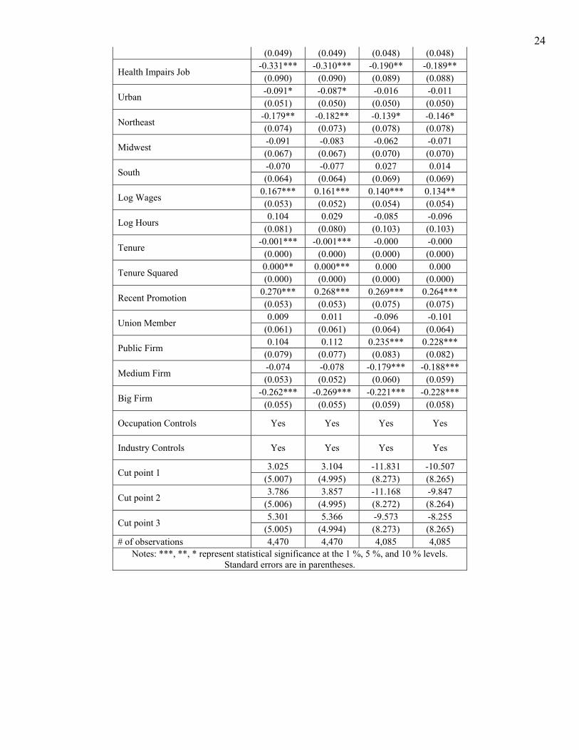
First, two waves in the NLSY, 1996 and 2004, are used to display the range of

results that can come from simple cross-section ordered-probit regressions. Table 2

reports the results of two separate regressions estimated for each NLSY wave. The first

includes the eight particular fringe benefits as dummy independent variables while the

second includes as dummies the number of fringe benefits each worker claims to have.

The estimated impact of the particular fringe benefits lack wide-ranging significance in

determining fringe benefits, especially when comparing the results across the two NLSY

waves. For instance, pensions lose their significantly positive impact on job satisfaction

from 1996 to 2004, employer provided health insurance has a significant negative

relationship with job satisfaction in 2004 but not in 1996 and the coefficient on employer

offered vacation days switches sign between the 1996 and 2004 cross-sections. In

addition, the fringe benefit count variables show no significant relationship with job

14

satisfaction in 1996 except for those workers who claim to have seven or eight fringe

benefits. On the other hand in 2004, all workers with at least one fringe benefit enjoy

significantly increased job satisfaction, except for those workers with three fringe

benefits. Thus the results from cross-section estimates of individual waves in the NLSY

are inconclusive in determining the relationship between fringe benefits and job

satisfaction.

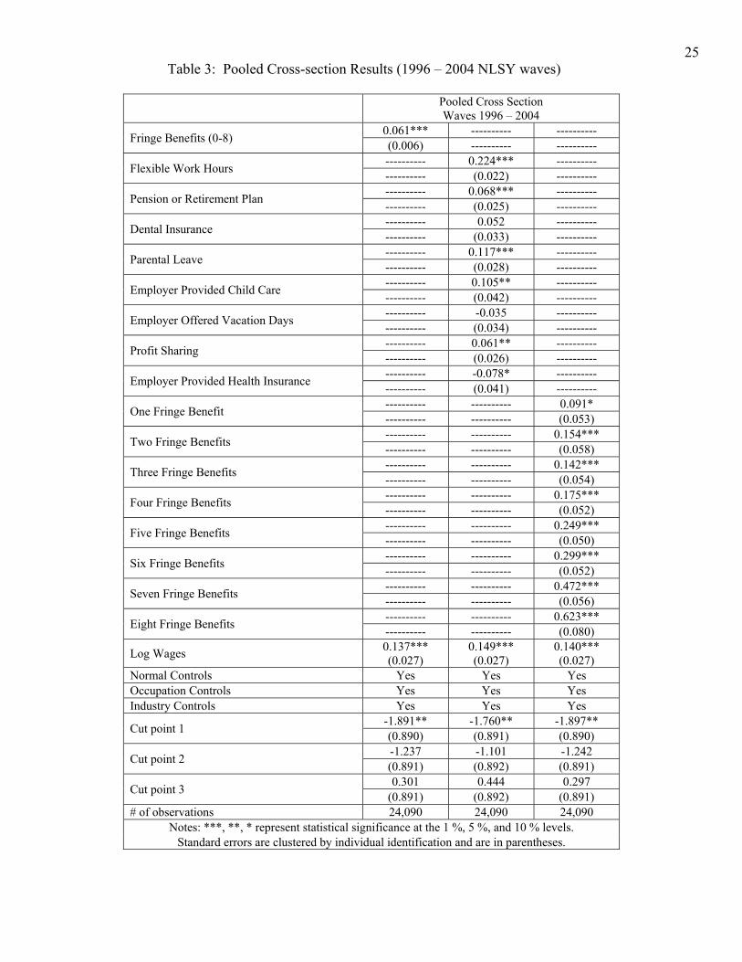
It is possible that the individual waves of the NLSY exhibit insufficient variation

between fringe benefits and job satisfaction to produce accurate results. Thus to increase

the estimation sample size, waves 1996 – 2004 of the NLSY are pooled as these are the

five most recent waves that contain all the necessary information regarding the eight

fringe benefits of interest. Since the pooled data is longitudinal though, it is necessary to

control for the serial-correlation that may exist between the individual observations

across the five waves. The standard errors are therefore clustered according to

individuals in the dataset. Table 3 displays these results.

With the greater sample size, the cross-section estimation reveals that five out of

eight fringe benefits significantly and positively impact job satisfaction with only one,

health insurance, showing a negative significant coefficient. Health insurance may

decrease job satisfaction if the worker’s spouse already has it, effectively lowering the

worker’s wages for a duplicate fringe benefit. Also, health insurance may create job lock

if an employee cannot leave an unsatisfactory job and health insurance is not available at

other, more appealing jobs. As well as the individual fringe benefit results, the

coefficients on the fringe benefit quantity dummies also tell a convincing story. The

15

estimated impact of fringe benefits on job satisfaction generally grows both in size and

significance as the number of fringe benefits increases.

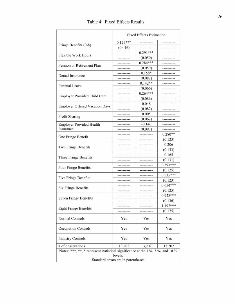
The pooled cross-section results may not be due to the increase in measurable

variation from the larger sample size but rather from unobservable individual

characteristics that are correlated with both job satisfaction and fringe benefits, biasing

the estimated coefficients. A fixed effects regression is therefore used to control for the

unmeasured individual characteristics. This regression estimates the impact of fringe

benefits on job satisfaction after dropping all the variables from the data that do not

exhibit any variation across the five NLSY waves. Since unmeasured individual

characteristics are assumed to not vary across the five waves, they are dropped from the

regression as well. Therefore, the potentially biasing impacts of fixed effects are

controlled for and the resulting coefficients are displayed in Table 4.

Five fringe benefits remain significant and positive determinants of job

satisfaction. These include flexible work hours, dental insurance, pension plans, parental

leave and employer provided child care. Although losing its significance, health

insurance remains negatively related to job satisfaction. In addition, most of the fringe

benefit dummies reflecting the quantity of benefits retain their positive and significant

relationship with job satisfaction. Only the quantity dummies representing two and three

fringe benefits no longer have significant coefficients. Thus the unobservable individual

characteristics of workers do not greatly alter the estimated impact of fringe benefits on

job satisfaction.

Both the fixed effects regression and the pooled cross-section regression provide

similar results. Fringe benefits are a significantly positive determinant of job satisfaction.

16

Yet workers’ job satisfaction and fringe benefit provisions may be simultaneously

determined. In other words, unmeasured determinants of job satisfaction might also

determine fringe benefits for employees. Normally an instrument is used in a two-stage

least squares procedure to correct for endogeneity between the dependent variable and

independent variable of interest. However in this case, job satisfaction and fringe benefit

variables are categorical rather than continuous and so it is problematic to employ the

same two-stage least squares approach. Rather, a recursive bivariate probit approach can

detect the presence of endogeneity by testing if the cross-equation correlation between

the identification equation and the job satisfaction equation is significantly different from

zero.

The chosen instrument is a dummy that equals one if the respondent or spouse has

any other sources of income and zero otherwise. This dummy is correlated with fringe

benefits provision but not with job satisfaction and is included in the fringe benefit

structural equation but not in the job satisfaction equation. First the dummy variables,

each representing at minimum how many fringe benefits employees claim to have are

treated as the endogenous independent dummy variable and second, each of the eight

individual fringe benefits is treated separately as the endogenous dummy. In all, sixteen

separate recursive bivariate probit regressions are used to test for potential endogeneity

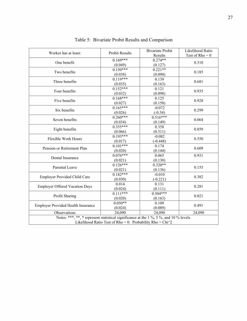
between fringe benefits and job satisfaction. The results of these bivariate probit

estimations are listed in Table 5.

The first column shows the pooled cross-section result when job satisfaction is a

dichotomous dummy and a probit estimation is used only for each individual measure of

benefits as the independent variable of interest. The second column shows the estimated

17

coefficient of each fringe benefit measure on job satisfaction within the recursive

bivariate probit framework. In this way job satisfaction and each fringe benefit dummy

variable are simultaneously determined within the model, effectively controlling for

potential endogeneity. The third column shows the results of the likelihood ratio test for

the cross-equation correlation equal to zero. If the likelihood ratio test reflects that this

correlation is not significantly different than zero, we cannot accept the hypothesis of

endogeneity. Indeed, all but two of the correlations are far from a significance level of

5%. Only profit sharing reports a cross-equation correlation that is significantly different

from zero at the 5% significance level while the fringe benefit dummy reflecting workers

with at least seven fringe benefits has a cross-equation correlation significantly different

from zero at the 10% level. Although these two show evidence of endogeneity, their

coefficients are still positive and significant, confirming that the relationship still remains

even after controlling for endogeneity. Thus the endogenous relationship between fringe

benefits and job satisfaction is not a problematic issue in this NLSY data. Therefore, the

estimates obtained from the pooled cross-section data should be used to study the impact

of fringe benefits on job satisfaction.

5. Further Robustness Tests

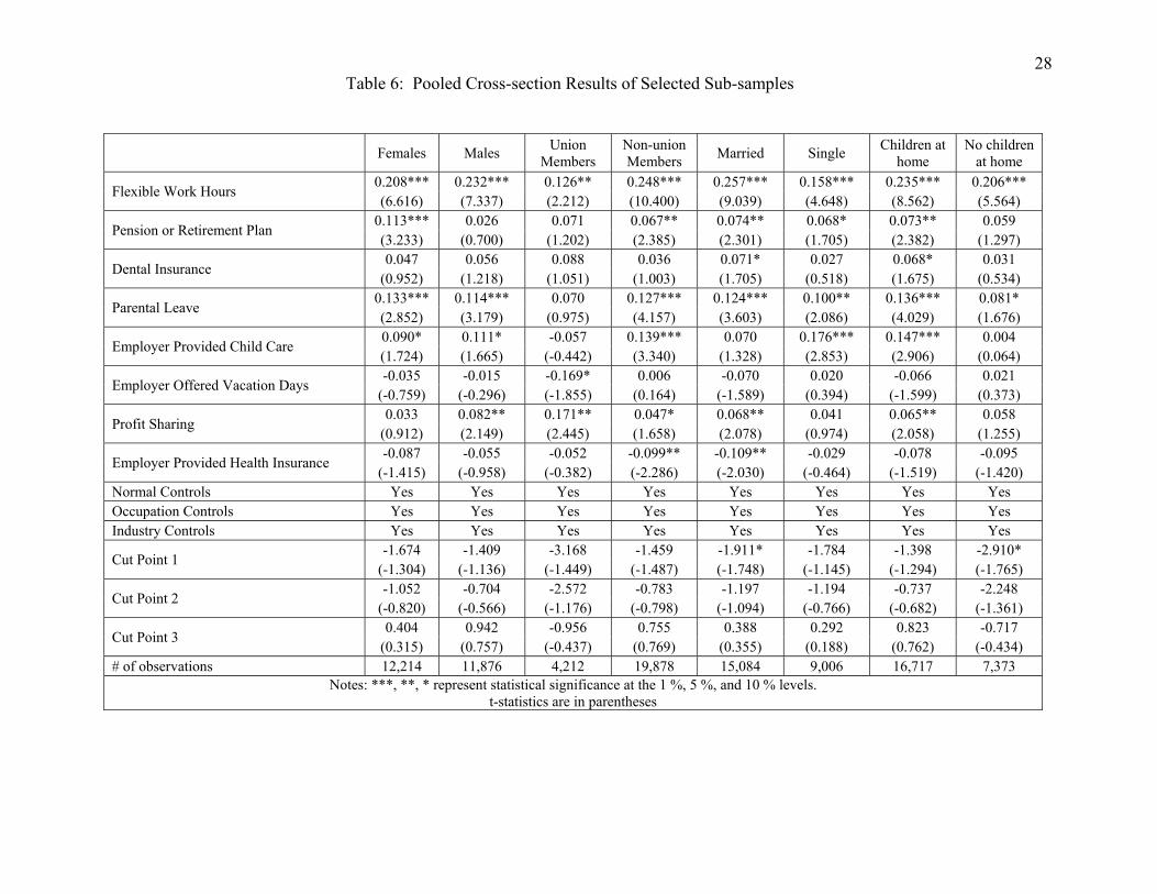
To examine the prevalence of the role of fringe benefits, several further tests are

undertaken. The pooled dataset is split four ways and cross-sections are estimated for

each sub-sample. The results are shown in Table 6. First, the sample is split by gender

and pooled cross-sections of each sub-sample are estimated. Both males and females

seem to value similar fringe benefits including flexible work hours, parental leave and

18

employer provided child care. However, only females significantly value pensions while

only males value profit sharing8. Therefore fringe benefits are significant determinants of

job satisfaction for both males and females.

Next, the impact of fringe benefits on job satisfaction for union members is

compared to non-union members. As a result of collective bargaining, union members

generally have more fringe benefits than non-union members. Specifically though, non-

union workers value fringe benefits more than union workers. Both groups value flexible

work hours and profit sharing, yet only non-union workers additionally value pensions,

parental leave and employer provided childcare. Thus it is evident that fringe benefits are

not as important in determining the job satisfaction of union workers as they are for non-

union workers. It may be that union workers take fringe benefit provision for granted due

in part to their bargaining power, effectively reducing the relationship between fringe

benefits and job satisfaction9.

The sample is then split by marital status indicated at the time of the respondent’s

interview. Flexible work hours, pensions and parental leave are positively and

significantly related to job satisfaction for both groups, yet interesting differences remain.

First, employer provided child care is only important for single workers. After all,

married workers may not need employer provided child care if their spouse has time to

look after the children. Second, employer provided health insurance is significantly and

negatively related to job satisfaction only for married workers. This may be a result of

the wasteful duplication of fringe benefit provision among spouses. If a spouse has

health insurance then the worker’s health insurance is useless and needlessly reduces

wages resulting in lower job satisfaction.

19

Finally the sample is split between workers who have children at home and those

that do not. Fringe benefits are often suited for workers with families so those with

dependents at home are more likely to value fringe benefits than those that do not. As

anticipated, six of the eight fringe benefits positively impact job satisfaction of workers

with children at home while only two significantly impact the job satisfaction of those

with no dependents at home.

6. Conclusion

Fringe benefits make up a significant portion of compensation packages paid to

employees, but their impact on worker job satisfaction has yet to be given much attention.

Fringe benefits can affect job satisfaction in opposing ways. First of all, since fringe

benefits are generally less taxed than wages, they can be purchased at less cost through an

employer than if bought on the market. Second, fringe benefits are often desirable pieces

of compensation packages and so increase job satisfaction. However, if spousal

compensation packages already provide particular fringe benefits, those offered by an

employer might be considered wasteful. Since past research has shown that wages often

suffer in exchange for fringe benefits, those that are wasteful may decrease job

satisfaction. Finally workers can feel locked in to a particular job or employer if the

fringe benefits they need or desire cannot be gained at a better, more satisfying job

elsewhere. This job-lock can decrease job satisfaction.

In order to estimate the relationship between fringe benefits and job satisfaction,

five waves of the NLSY are used first in cross-section estimations of the individual

waves, second as a pooled dataset and then finally as a panel dataset utilizing the

20

longitudinal nature of the survey. Eight dummy variables representing individual fringe

benefits but also quantities of benefits employees claim to have act as the independent

variables of interest in the models.

The results from individual NLSY wave cross-section estimations do not provide

convincing evidence that fringe benefits act as determinants of job satisfaction. Although

the pooled cross-section estimation offers more compelling results, unobservable

characteristics not measured and therefore not included in the cross-section estimation

can bias the estimated impact of fringe benefits on job satisfaction. After controlling for

the potentially biasing unobservable individual characteristics using a fixed effects

regression, most of the results from the pooled cross-section estimation carry over to the

fixed effects estimation. Therefore fixed effects do not seem to compromise the

significant relationship between fringe benefits and job satisfaction.

Moreover, fringe benefits may be simultaneously determined with job

satisfaction. If fringe benefits are indeed endogenous, then their estimated impact on job

satisfaction will be biased. Using a recursive bivariate probit approach, this endogenous

relationship is tested using the likelihood ratio test of the cross-equation correlation of the

structural equations for job satisfaction and fringe benefit provision. Most of the

correlations are indeed not significantly different from zero, confirming that endogeneity

is not a problem in this dataset. Therefore, the pooled cross-section estimates are

accurate depictions of the impact that fringe benefits have on job satisfaction.

To further investigate the proposition that fringe benefits are significant

determinants of job satisfaction, cross-sections of the pooled dataset are estimated for

four different sub-samples. First, the results suggest there is no significant difference

21

between the preferences for fringe benefits between males and females. However, the

results indicate both union workers and workers with no children living at home do not

value fringe benefits as much as their respective sub-sample counterparts. Finally, the

estimated coefficients on fringe benefits in job satisfaction estimations exhibit interesting

differences between that of married and single workers. Health insurance is negatively

related to job satisfaction for married workers while employer provided child care is only

valuable for single workers.

There is much room for expansion in the job satisfaction literature, including

topics dealing with fringe benefits as this paper suggests. Overall, fringe benefits play a

significant role in determining employee job satisfaction. It is therefore important to

further study this relationship in detail.

22Table 1: Sample Means and Standard Deviations by Number of Fringe Benefits

Whole No 1 or 2 3 or 4 5 or 6 7 or 8

Sample Fringes Fringes Fringes Fringes Fringes Number of Observations 24,090 1,409 3,153 4,762 11,087 3,679

Job Satisfaction = 1 if very satisfied, 0 otherwise 3.369 3.218 3.304 3.336 3.384 3.477 (0.692) (0.778) (0.751) (0.704) (0.672) (0.630)

Flexible Work Hours = 1 if employer allows flexible work hours or schedule

0.537 ---------- 0.513 0.334 0.559 0.958 (0.499) ---------- (0.500) (0.472) (0.497) (0.200)

Pension = 1 if employer provides a pension or retirement plan 0.608 ---------- 0.086 0.368 0.816 0.973 (0.488) ---------- (0.280) (0.482) (0.387) (0.163)

Dental Insurance = 1 if employer offers dental insurance 0.700 ---------- 0.030 0.580 0.934 0.997 (0.458) ---------- (0.170) (0.494) (0.249) (0.057)

Parental Leave = 1 if employer allows maternity / paternity leave 0.702 ---------- 0.091 0.594 0.915 0.994 (0.457) ---------- (0.288) (0.491) (0.279) (0.077)

Child Care = 1if employer provides or subsidizes child care 0.089 ---------- 0.007 0.015 0.049 0.408 (0.285) ---------- (0.081) (0.121) (0.217) (0.491)

Vacation Days = 1 if worker has paid vacation days 0.829 ---------- 0.527 0.812 0.973 0.997 (0.376) ---------- (0.499) (0.391) (0.163) (0.052)

Profit Sharing = 1 if employer offers profit sharing 0.270 ---------- 0.016 0.069 0.269 0.856 (0.444) ---------- (0.124) (0.254) (0.443) (0.351)

Health Insurance = 1 if employer offers off the job health insurance

0.807 ---------- 0.184 0.880 0.992 1.000 (0.394) ---------- (0.387) (0.325) (0.087) (0.016)

Female = 1 if respondent is female 0.507 0.479 0.501 0.498 0.505 0.540 (0.500) (0.500) (0.500) (0.500) (0.500) (0.498)

Black = 1 if respondent is Black 0.294 0.378 0.290 0.265 0.280 0.348 (0.456) (0.485) (0.454) (0.441) (0.449) (0.476)

Hispanic = 1 if respondent is Hispanic 0.192 0.221 0.206 0.204 0.189 0.164 (0.394) (0.415) (0.405) (0.403) (0.392) (0.370)

High School Education = 1 if highest grade completed = 12 0.447 0.494 0.517 0.469 0.428 0.403 (0.497) (0.500) (0.500) (0.499) (0.495) (0.490)

College Education = 1 if highest grade completed >12 & < 17 0.368 0.207 0.266 0.324 0.411 0.442 (0.482) (0.405) (0.442) (0.468) (0.492) (0.497)

Post College Education = 1if highest grade completed > 16 0.089 0.023 0.030 0.091 0.106 0.113 (0.285) (0.149) (0.172) (0.287) (0.308) (0.316)

Age = age of respondent 38.789 38.370 38.501 38.596 38.931 39.016 (3.575) (3.456) (3.522) (3.558) (3.595) (3.584)

Health Impairs Job = 1if respondent has any health issues that limits job performance

0.070 0.145 0.114 0.077 0.052 0.046 (0.255) (0.353) (0.318) (0.267) (0.222) (0.209)

Married = 1if respondent is currently married 0.626 0.424 0.543 0.626 0.666 0.654 (0.484) (0.494) (0.498) (0.484) (0.472) (0.476)

Urban Residence = 1 if respondent lives in an urban area 0.744 0.734 0.713 0.730 0.745 0.787 (0.437) (0.442) (0.452) (0.444) (0.436) (0.410)

Hourly Wage = wage based on respondent's usual wage, time unit of pay and usual hours worked per time unit

16.343 9.593 10.957 14.638 18.042 20.632 (15.080) (7.698) (10.045) (11.187) (15.092) (21.414)

Weekly Hours = usual hours worked per week 41.416 40.013 38.984 41.310 42.025 42.340 (9.621) (13.665) (11.591) (9.791) (8.385) (8.704)

Tenure = tenure in weeks with employer as of interview date 332.448 115.464 184.642 319.245 389.041 388.766 (308.955) (158.264) (219.436) (298.624) (320.290) (315.998)

Recent Promotion = 1 if recent position change was a promotion 0.154 0.048 0.089 0.124 0.173 0.235 (0.361) (0.214) (0.285) (0.329) (0.378) (0.424)

Union Member = 1 if respondent is a member of a labor union 0.175 0.044 0.048 0.209 0.229 0.126 (0.380) (0.205) (0.214) (0.407) (0.420) (0.332)

Public Employer = 1 if respondent works for the government 0.183 0.077 0.075 0.202 0.253 0.080 (0.386) (0.267) (0.263) (0.402) (0.434) (0.272)

Medium Firm = 1 if respondent has between 50 and 249 coworkers

0.264 0.120 0.130 0.286 0.308 0.276 (0.441) (0.325) (0.336) (0.452) (0.462) (0.447)

Big Firm = 1if respondent has greater than 250 coworkers 0.303 0.128 0.105 0.190 0.367 0.491 (0.459) (0.335) (0.307) (0.393) (0.482) (0.500)

23Table 2: 1996 and 2004 NLSY Cross-section Results

1996 NLSY Wave 2004 NLSY Wave

Flexible Work Hours 0.237*** ---------- 0.162*** ---------- (0.043) ---------- (0.047) ----------

Pension or Retirement Plan 0.114** ---------- 0.042 ---------- (0.052) ---------- (0.059) ----------

Dental Insurance 0.042 ---------- 0.028 ----------

(0.059) ---------- (0.075) ----------

Parental Leave 0.148*** ---------- 0.196*** ---------- (0.054) ---------- (0.066) ----------

Employer Provided Child Care 0.125 ---------- 0.114 ----------

(0.078) ---------- (0.081) ----------

Employer Offered Vacation Days -0.142** ---------- 0.145* ---------- (0.065) ---------- (0.082) ----------

Profit Sharing 0.048 ---------- 0.081 ----------

(0.050) ---------- (0.054) ---------- Employer Provided Health Insurance

-0.082 ---------- -0.172* ---------- (0.076) ---------- (0.094) ----------

One Fringe Benefit ---------- -0.002 ---------- 0.288* ---------- (0.115) ---------- (0.149)

Two Fringe Benefits ---------- 0.173 ---------- 0.361** ---------- (0.118) ---------- (0.153)

Three Fringe Benefits ---------- -0.092 ---------- 0.341** ---------- (0.110) ---------- (0.147)

Four Fringe Benefits ---------- 0.069 ---------- 0.229 ---------- (0.106) ---------- (0.139)

Five Fringe Benefits ---------- 0.166 ---------- 0.442*** ---------- (0.104) ---------- (0.135)

Six Fringe Benefits ---------- 0.171 ---------- 0.462*** ---------- (0.107) ---------- (0.135)

Seven Fringe Benefits ---------- 0.430*** ---------- 0.674*** ---------- (0.116) ---------- (0.142)

Eight Fringe Benefits ---------- 0.543*** ---------- 0.565*** ---------- (0.169) ---------- (0.184)

Female 0.023 0.046 0.051 0.065

(0.051) (0.050) (0.054) (0.054)

Black -0.134*** -0.149*** -0.014 -0.009

(0.050) (0.050) (0.053) (0.053)

Hispanic 0.088 0.069 0.141** 0.145**

(0.057) (0.056) (0.058) (0.058)

High School -0.118 -0.091 -0.062 -0.055 (0.077) (0.076) (0.085) (0.085)

College -0.111 -0.073 -0.179* -0.173* (0.086) (0.085) (0.092) (0.092)

Post College 0.055 0.104 -0.027 -0.017

(0.119) (0.118) (0.119) (0.119)

Age 0.276 0.297 -0.458 -0.398

(0.285) (0.284) (0.382) (0.382)

Age Squared -0.387 -0.416 0.538 0.468 (0.407) (0.406) (0.441) (0.441)

Married 0.079 0.084* 0.075 0.076

24(0.049) (0.049) (0.048) (0.048)

Health Impairs Job -0.331*** -0.310*** -0.190** -0.189**

(0.090) (0.090) (0.089) (0.088)

Urban -0.091* -0.087* -0.016 -0.011 (0.051) (0.050) (0.050) (0.050)

Northeast -0.179** -0.182** -0.139* -0.146* (0.074) (0.073) (0.078) (0.078)

Midwest -0.091 -0.083 -0.062 -0.071 (0.067) (0.067) (0.070) (0.070)

South -0.070 -0.077 0.027 0.014 (0.064) (0.064) (0.069) (0.069)

Log Wages 0.167*** 0.161*** 0.140*** 0.134** (0.053) (0.052) (0.054) (0.054)

Log Hours 0.104 0.029 -0.085 -0.096

(0.081) (0.080) (0.103) (0.103)

Tenure -0.001*** -0.001*** -0.000 -0.000

(0.000) (0.000) (0.000) (0.000)

Tenure Squared 0.000** 0.000*** 0.000 0.000 (0.000) (0.000) (0.000) (0.000)

Recent Promotion 0.270*** 0.268*** 0.269*** 0.264*** (0.053) (0.053) (0.075) (0.075)

Union Member 0.009 0.011 -0.096 -0.101

(0.061) (0.061) (0.064) (0.064)

Public Firm 0.104 0.112 0.235*** 0.228***

(0.079) (0.077) (0.083) (0.082)

Medium Firm -0.074 -0.078 -0.179*** -0.188*** (0.053) (0.052) (0.060) (0.059)

Big Firm -0.262*** -0.269*** -0.221*** -0.228***

(0.055) (0.055) (0.059) (0.058)

Occupation Controls Yes Yes Yes Yes

Industry Controls Yes Yes Yes Yes

Cut point 1 3.025 3.104 -11.831 -10.507

(5.007) (4.995) (8.273) (8.265)

Cut point 2 3.786 3.857 -11.168 -9.847

(5.006) (4.995) (8.272) (8.264)

Cut point 3 5.301 5.366 -9.573 -8.255

(5.005) (4.994) (8.273) (8.265) # of observations 4,470 4,470 4,085 4,085

Notes: ***, **, * represent statistical significance at the 1 %, 5 %, and 10 % levels. Standard errors are in parentheses.

25Table 3: Pooled Cross-section Results (1996 – 2004 NLSY waves)

Pooled Cross Section

Waves 1996 – 2004

Fringe Benefits (0-8) 0.061*** ---------- ---------- (0.006) ---------- ----------

Flexible Work Hours ---------- 0.224*** ---------- ---------- (0.022) ----------

Pension or Retirement Plan ---------- 0.068*** ---------- ---------- (0.025) ----------

Dental Insurance ---------- 0.052 ---------- ---------- (0.033) ----------

Parental Leave ---------- 0.117*** ---------- ---------- (0.028) ----------

Employer Provided Child Care ---------- 0.105** ---------- ---------- (0.042) ----------

Employer Offered Vacation Days ---------- -0.035 ---------- ---------- (0.034) ----------

Profit Sharing ---------- 0.061** ---------- ---------- (0.026) ----------

Employer Provided Health Insurance ---------- -0.078* ---------- ---------- (0.041) ----------

One Fringe Benefit ---------- ---------- 0.091* ---------- ---------- (0.053)

Two Fringe Benefits ---------- ---------- 0.154*** ---------- ---------- (0.058)

Three Fringe Benefits ---------- ---------- 0.142*** ---------- ---------- (0.054)

Four Fringe Benefits ---------- ---------- 0.175*** ---------- ---------- (0.052)

Five Fringe Benefits ---------- ---------- 0.249*** ---------- ---------- (0.050)

Six Fringe Benefits ---------- ---------- 0.299*** ---------- ---------- (0.052)

Seven Fringe Benefits ---------- ---------- 0.472*** ---------- ---------- (0.056)

Eight Fringe Benefits ---------- ---------- 0.623*** ---------- ---------- (0.080)

Log Wages 0.137*** (0.027)

0.149*** (0.027)

0.140*** (0.027)

Normal Controls Yes Yes Yes Occupation Controls Yes Yes Yes Industry Controls Yes Yes Yes

Cut point 1 -1.891** -1.760** -1.897** (0.890) (0.891) (0.890)

Cut point 2 -1.237 -1.101 -1.242 (0.891) (0.892) (0.891)

Cut point 3 0.301 0.444 0.297 (0.891) (0.892) (0.891)

# of observations 24,090 24,090 24,090 Notes: ***, **, * represent statistical significance at the 1 %, 5 %, and 10 % levels.

Standard errors are clustered by individual identification and are in parentheses.

26Table 4: Fixed Effects Results

Fixed Effects Estimation

Fringe Benefits (0-8) 0.125*** ---------- ---------- (0.016) ---------- ----------

Flexible Work Hours ---------- 0.291*** ---------- ---------- (0.050) ----------

Pension or Retirement Plan ---------- 0.284*** ---------- ---------- (0.059) ----------

Dental Insurance ---------- 0.158* ---------- ---------- (0.082) ----------

Parental Leave ---------- 0.142** ---------- ---------- (0.066) ----------

Employer Provided Child Care ---------- 0.264*** ---------- ---------- (0.086) ----------

Employer Offered Vacation Days ---------- 0.048 ---------- ---------- (0.082) ----------

Profit Sharing ---------- 0.005 ---------- ---------- (0.062) ----------

Employer Provided Health Insurance

---------- -0.146 ---------- ---------- (0.097) ----------

One Fringe Benefit ---------- ---------- 0.280** ---------- ---------- (0.123)

Two Fringe Benefits ---------- ---------- 0.206 ---------- ---------- (0.133)

Three Fringe Benefits ---------- ---------- 0.165 ---------- ---------- (0.131)

Four Fringe Benefits ---------- ---------- 0.393*** ---------- ---------- (0.125)

Five Fringe Benefits ---------- ---------- 0.535*** ---------- ---------- (0.123)

Six Fringe Benefits ---------- ---------- 0.654*** ---------- ---------- (0.125)

Seven Fringe Benefits ---------- ---------- 0.928*** ---------- ---------- (0.136)

Eight Fringe Benefits ---------- ---------- 1.192*** ---------- ---------- (0.175)

Normal Controls Yes Yes Yes

Occupation Controls Yes Yes Yes

Industry Controls Yes Yes Yes

# of observations 13,202 13,202 13,202 Notes: ***, **, * represent statistical significance at the 1 %, 5 %, and 10 %

levels. Standard errors are in parentheses

27

Table 5: Bivariate Probit Results and Comparison

Worker has at least: Probit Results Bivariate Probit Results

Likelihood Ratio Test of Rho = 0

One benefit 0.169*** (0.049)

0.274** (0.127) 0.310

Two benefits 0.150*** (0.038)

0.221** (0.090) 0.185

Three benefits 0.119*** (0.035)

0.139 (0.163) 0.681

Four benefits 0.152*** (0.032)

0.121 (0.098) 0.935

Five benefits 0.168*** (0.027)

0.125 (0.158) 0.928

Six benefits 0.165*** (0.026)

-0.072 (-0.34) 0.299

Seven benefits 0.260*** (0.034)

0.516*** (0.149) 0.064

Eight benefits 0.355*** (0.066)

0.358 (0.311) 0.859

Flexible Work Hours 0.193*** (0.017)

-0.082 (-0.448) 0.550

Pension or Retirement Plan 0.101*** (0.020)

0.174 (0.144) 0.609

Dental Insurance 0.076*** (0.021)

0.065 (0.130)

0.931

Parental Leave 0.126*** (0.021)

0.320** (0.136) 0.155

Employer Provided Child Care 0.182*** (0.030)

-0.010 (-0.221) 0.382

Employer Offered Vacation Days 0.014 (0.024)

0.131 (0.111) 0.281

Profit Sharing 0.111*** (0.020)

0.504*** (0.163) 0.021

Employer Provided Health Insurance 0.050** (0.024)

0.109 (0.089) 0.491

Observations 24,090 24,090 24,090 Notes: ***, **, * represent statistical significance at the 1 %, 5 %, and 10 % levels.

Likelihood Ratio Test of Rho = 0: Probability Rho > Chi^2

28Table 6: Pooled Cross-section Results of Selected Sub-samples

Females Males Union Members

Non-union Members Married Single Children at

home No children

at home

Flexible Work Hours 0.208*** 0.232*** 0.126** 0.248*** 0.257*** 0.158*** 0.235*** 0.206*** (6.616) (7.337) (2.212) (10.400) (9.039) (4.648) (8.562) (5.564)

Pension or Retirement Plan 0.113*** 0.026 0.071 0.067** 0.074** 0.068* 0.073** 0.059 (3.233) (0.700) (1.202) (2.385) (2.301) (1.705) (2.382) (1.297)

Dental Insurance 0.047 0.056 0.088 0.036 0.071* 0.027 0.068* 0.031

(0.952) (1.218) (1.051) (1.003) (1.705) (0.518) (1.675) (0.534)

Parental Leave 0.133*** 0.114*** 0.070 0.127*** 0.124*** 0.100** 0.136*** 0.081* (2.852) (3.179) (0.975) (4.157) (3.603) (2.086) (4.029) (1.676)

Employer Provided Child Care 0.090* 0.111* -0.057 0.139*** 0.070 0.176*** 0.147*** 0.004 (1.724) (1.665) (-0.442) (3.340) (1.328) (2.853) (2.906) (0.064)

Employer Offered Vacation Days -0.035 -0.015 -0.169* 0.006 -0.070 0.020 -0.066 0.021

(-0.759) (-0.296) (-1.855) (0.164) (-1.589) (0.394) (-1.599) (0.373)

Profit Sharing 0.033 0.082** 0.171** 0.047* 0.068** 0.041 0.065** 0.058

(0.912) (2.149) (2.445) (1.658) (2.078) (0.974) (2.058) (1.255)

Employer Provided Health Insurance -0.087 -0.055 -0.052 -0.099** -0.109** -0.029 -0.078 -0.095

(-1.415) (-0.958) (-0.382) (-2.286) (-2.030) (-0.464) (-1.519) (-1.420) Normal Controls Yes Yes Yes Yes Yes Yes Yes Yes Occupation Controls Yes Yes Yes Yes Yes Yes Yes Yes Industry Controls Yes Yes Yes Yes Yes Yes Yes Yes

Cut Point 1 -1.674 -1.409 -3.168 -1.459 -1.911* -1.784 -1.398 -2.910*

(-1.304) (-1.136) (-1.449) (-1.487) (-1.748) (-1.145) (-1.294) (-1.765)

Cut Point 2 -1.052 -0.704 -2.572 -0.783 -1.197 -1.194 -0.737 -2.248

(-0.820) (-0.566) (-1.176) (-0.798) (-1.094) (-0.766) (-0.682) (-1.361)

Cut Point 3 0.404 0.942 -0.956 0.755 0.388 0.292 0.823 -0.717

(0.315) (0.757) (-0.437) (0.769) (0.355) (0.188) (0.762) (-0.434) # of observations 12,214 11,876 4,212 19,878 15,084 9,006 16,717 7,373

Notes: ***, **, * represent statistical significance at the 1 %, 5 %, and 10 % levels. t-statistics are in parentheses

29

References Akerlof, G.A., A.K. Rose and J.L. Yellen (1988) “Job Switching and Job Satisfaction in the U.S. Labor Market”, Brookings Papers on Economic Activity, Volume 2, pp. 495-582. Alpert, W. T. (1987) “An Analysis of Fringe Benefits Using Time-series Data”, Applied Economics. Vol. 19, pp. 1-16. Artz, B. (2008) “The Role of Firm Size and Performance Pay in Determining Employee Job Satisfaction”, Labour: Review of Labor Economics and Industrial Relations, Forthcoming, June 2008. Baughman, R., D. DiNardi and D. Holtz-Eakin (2003) “Productivity and Wage Effects of “Family-friendly” Fringe Benefits”. International Journal of Manpower. Vol. 24, No. 3, pp. 247-259. Belfield, C.R. and R.D.F. Harris (2002) “How well do theories of job matching explain variations in job satisfaction across education levels? Evidence for UK graduates.” Applied Economics. Vol. 34 No. 5 pp. 535-548. Bender, K.A., S.M. Donohue and J.S. Heywood (2005) “Job Satisfaction and Gender Segregation” Oxford Economic Papers Vol. 57 pp. 479-496. Bender, K.A. and J.S. Heywood (2006) “Job Satisfaction of the Highly Educated: The Role of Gender, Academic Tenure and Earnings” Scottish Journal of Political Economy Vol. 52 No. 2 pp. 253-279. Benz, M. (2005) “Not for the Profit, but for the Satisfaction? Evidence on Worker Well-Being in Non-Profit Firms” KYKLOS Vol. 58 No. 2 pp. 155-176 Bryson, A., L. Cappellari and C. Lucifora (2005) “Why so Unhappy? The Effects of Unionization on Job Satisfaction” CESIFO Working Paper No. 1419 Clark, A. (2003) “Looking for Labor Market Rents Using Subjective Data” Working Paper, September 2003. Clegg, C.W. (1983) “Psychology of Employee Lateness, Absence and Turnover: A Methodological Critique and an Empirical Study”, Journal of Applied Psychology, Vol. 68, pp. 88-101. Creedy, J and K. Whitfield (1988) “The Economic Analysis of Internal Labour Markets” Bulletin of Economic Research, Vol. 40. No. 4 pp. 247-269.

30

Donohue, S.M. and J.S. Heywood (2004) “Job Satisfaction and Gender: An Expanded Specification from the NLSY” International Journal of Manpower Vol. 25 No. 2 pp. 211-234. Freeman, R.B. (1978) “Job Satisfaction as an Economic Variable”, The American Economic Review Vol. 68. No. 2. pp. 135-141. Heywood, J.S., W.S. Siebert and X. Wei (2002) “Worker Sorting and Job Satisfaction: The Case of Union and Government Jobs” Industrial and Labor Relations Review Vol. 55 No. 4 pp. 595-609. Heywood, J.S. and X. Wei (2006) “Performance Pay and Job Satisfaction” Journal of Industrial Relations, Vol. 48. No. 4. pp. 523-540. Jensen, G.A. and M. A. Morrisey (2001) “Endogenous Fringe Benefits, Compensating Wage Differentials and Older Workers” International Journal of Health Care and Economics Sep – Dec 2001, Vol. 1. pp. 203 – 226. Kiker, B.F. and S.L.W. Rhine (1986) “Fringe Benefits and the Earnings Equation” Journal of Human Resources Vol. 22 No. 1 pp.126–137. Luchak, A.A. and I.R. Gellatly (2002) “How Pension Accrual Affects Job Satisfaction” Journal of Labor Research Vol. 23 No. 1 pp.145-162. Maddala, G.S. (1987) “Limited Dependent Variable Models Using Panel Data” The Journal of Human Resources, Vol. 22, No. 3, pp. 307-338. McCausland, W.D., Pouliakas, K., and Theodossiou, I. (2005) “Some are Punished and Some are Rewarded: A Study of the Impact of Performance Pay on Job Satisfaction”. International Journal of Manpower. Vol. 26 No. 7/8. pp. 636-659. Mangione, T.W. and R.P. Quinn (1975) “Job Satisfaction, Counter-Productive Behavior and Drug Use at Work”, Journal of Applied Psychology, Vol. 60, pp. 114-116. McEvoy, G.M. and W.F. Cascio (1985) “Strategies for Reducing Employee Turnover: A Meta Analysis”, Journal of Applied Psychology, Vol. 70 pp. 342-353. McFadden, D. (1973) “Conditional Logit Analysis of Qualitative Choice Behavior” Frontiers in Economics, Edited by P. Zarembka. New York: Academic Press. Monfardini, C and R. Radice (2008) “Testing Exogeneity in the Bivariate Probit Model: A Monte Carlo Study” Oxford Bulletin of Economics and Statistics Vol. 70, No. 2 pp. 271 – 282.

31

Saltzstein, A.L., Y. Ting and G.H. Saltzstein (2001) “Work-Family Balance and Job Satisfaction: The Impact of Family-Friendly Policies on Attitudes of Federal Government Employees” Public Administration Review Vol. 61 No. 4 pp.452-467. Uppal, S. (2005) “Disability, Workplace Characteristics and Job Satisfaction” International Journal of Manpower Vol. 26 No. 4 pp. 336-349. Vieira, J.C., A. Menezes and P. Gabriel (2005) “Low Pay, Higher Pay and Job Quality: Empirical Evidence for Portugal” Applied Economics Letters Vol. 12 pp. 505-511 Weiss, A. (1984) “Determinants of Quit Behavior”, Journal of Labor Economics, Vol. 2. No. 3. pp. 371-387. Woodbury, S. (1983) “Substitution Between Wage and Nonwage Benefits”. American Economic Review. Vol. 73, No. 1. pp. 166-182.

32

Appendix 1: Regression Comparison

Ordered Probit

Ordered Logit

Binary Logit

One Fringe Benefit 0.091* 0.166* 0.133 (0.053) (0.093) (0.094)

Two Fringe Benefits 0.154*** 0.290*** 0.267*** (0.058) (0.101) (0.102)

Three Fringe Benefits 0.142*** 0.233** 0.140 (0.054) (0.095) (0.099)

Four Fringe Benefits 0.175*** 0.295*** 0.229** (0.052) (0.093) (0.095)

Five Fringe Benefits 0.249*** 0.417*** 0.358*** (0.050) (0.089) (0.091)

Six Fringe Benefits 0.299*** 0.502*** 0.424*** (0.052) (0.091) (0.094)

Seven Fringe Benefits 0.472*** 0.794*** 0.711*** (0.056) (0.098) (0.102)

Eight Fringe Benefits 0.623*** 1.071*** 1.001*** (0.080) (0.135) (0.138)

Female 0.076*** 0.160*** 0.189*** (0.028) (0.049) (0.051)

Black -0.076*** -0.123** -0.116**

(0.029) (0.049) (0.051)

Hispanic 0.108*** 0.180*** 0.184*** (0.032) (0.055) (0.057)

High School -0.079* -0.126* -0.113 (0.043) (0.074) (0.080)

College -0.131*** -0.213*** -0.200**

(0.046) (0.080) (0.086)

Post College -0.011 0.011 0.055 (0.065) (0.110) (0.114)

Age 0.009 0.030 0.055

(0.045) (0.076) (0.080)

Age Squared -0.011 -0.039 -0.069 (0.058) (0.098) (0.103)

Married 0.068*** 0.098** 0.087** (0.024) (0.042) (0.044)

Health Impairs Job -0.166*** -0.263*** -0.159**

(0.041) (0.074) (0.073)

Urban -0.071*** -0.113*** -0.092**

(0.025) (0.042) (0.045)

Northeast -0.128*** -0.210*** -0.189**

(0.043) (0.074) (0.077)

Midwest -0.062 -0.110* -0.116* (0.039) (0.066) (0.069)

33

South -0.002 -0.000 0.012 (0.037) (0.063) (0.065)

Log Wages 0.140*** 0.242*** 0.231*** (0.027) (0.045) (0.047)

Log Hours -0.037 -0.030 0.004 (0.040) (0.070) (0.072)

Tenure -0.001*** -0.001*** -0.001***

(0.000) (0.000) (0.000)

Tenure Squared 0.000*** 0.000*** 0.000*** (0.000) (0.000) (0.000)

Recent Promotion 0.224*** 0.368*** 0.361*** (0.026) (0.044) (0.046)

Union Member -0.019 -0.009 -0.001 (0.035) (0.059) (0.063)

Public Firm 0.256*** 0.415*** 0.405*** (0.043) (0.072) (0.076)

Medium Firm -0.149*** -0.265*** -0.278***

(0.029) (0.048) (0.051)

Big Firm -0.256*** -0.453*** -0.463***

(0.030) (0.052) (0.054) Occupation Controls Yes Yes Yes Industry Controls Yes Yes Yes

Constant ---------- ---------- -1.516 ---------- ---------- (1.581)

Cut point 1 -1.897** -3.162** ---------- (0.890) (1.511) ----------

Cut point 2 -1.242 -1.726 ---------- (0.891) (1.512) ----------

Cut point 3 0.297 0.946 ----------

(0.891) (1.513) ---------- # of observations 24,090 24,090 24,090 Notes: ***, **, * represent statistical significance at the 1 %, 5 %, and 10

% levels. Standard errors are in parentheses.

34

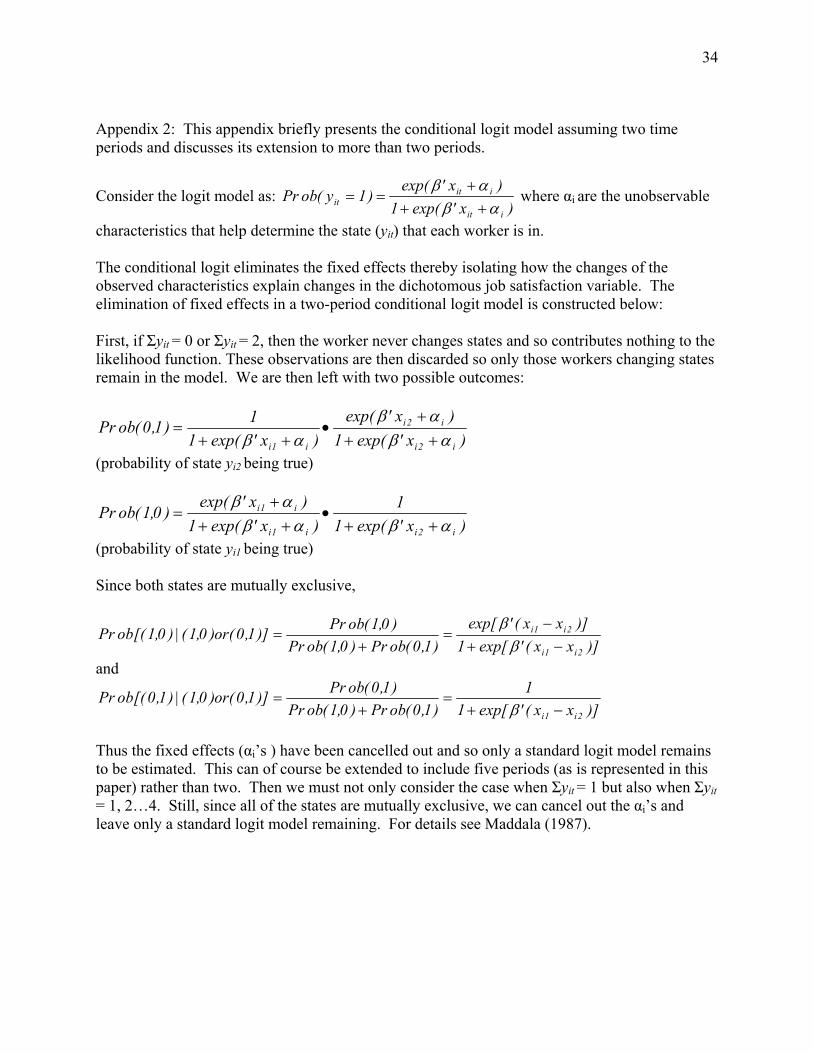
Appendix 2: This appendix briefly presents the conditional logit model assuming two time periods and discusses its extension to more than two periods.

Consider the logit model as: )x'exp(1

)x'exp()1y(obPr

iit

iitit αβ

αβ++

+== where αi are the unobservable

characteristics that help determine the state (yit) that each worker is in. The conditional logit eliminates the fixed effects thereby isolating how the changes of the observed characteristics explain changes in the dichotomous job satisfaction variable. The elimination of fixed effects in a two-period conditional logit model is constructed below: First, if Σyit = 0 or Σyit = 2, then the worker never changes states and so contributes nothing to the likelihood function. These observations are then discarded so only those workers changing states remain in the model. We are then left with two possible outcomes:

)x'exp(1)x'exp(

)x'exp(11)1,0(obPr

i2i

i2i

i1i αβαβ

αβ +++

•++

=

(probability of state yi2 being true)

)x'exp(11

)x'exp(1)x'exp(

)0,1(obPri2ii1i

i1i

αβαβαβ

++•

+++

=

(probability of state yi1 being true) Since both states are mutually exclusive,

)]xx('exp[1)]xx('exp[

)1,0(obPr)0,1(obPr)0,1(obPr)]1,0(or)0,1(|)0,1[(obPr

2i1i

2i1i

−+−

=+

=β

β

and

)]xx('exp[11

)1,0(obPr)0,1(obPr)1,0(obPr)]1,0(or)0,1(|)1,0[(obPr

2i1i −+=

+=

β

Thus the fixed effects (αi’s ) have been cancelled out and so only a standard logit model remains to be estimated. This can of course be extended to include five periods (as is represented in this paper) rather than two. Then we must not only consider the case when Σyit = 1 but also when Σyit = 1, 2…4. Still, since all of the states are mutually exclusive, we can cancel out the αi’s and leave only a standard logit model remaining. For details see Maddala (1987).

35

Endnotes: 1 The definition of civilians includes all workers in the private non-farm economy, excluding

households, and the public sector, excluding federal government employees.

2 While most studies fail to control for fixed effects, some do not. These include Vieira,

Menezes and Gabriel (2005), Donohue and Heywood (2004), Heywood, Siebert and Wei (2002),

Benz (2005) and Heywood and Wei (2006), although some do not report coefficients on fringe

benefits after controlling for fixed effects.

3 This result is even more impressive since all of the survey respondents in the study are union

workers. Union workers are generally more difficult to layoff due to their relative labor market

power. So union workers feeling more risk of layoff from higher pension accruals is a striking

result indeed.

4 Vieira, Menezes and Gabriel (2005) find that employer provided health insurance instead

increases job satisfaction. The authors use waves 1997-1999 of the European Community

Household Panel for Portugal. The result comes from a random effects ordered probit

estimation. The authors assume heterogeneity across individuals in their unobserved

characteristics, but by using random effects panel estimation, assume that these characteristics

could also change across time periods. Fixed effects panel estimation assumes that unobservable

worker characteristics vary across individuals but not across time periods for each individual.

5 Saltzstein, Ting and Saltzstein (2001) note that while family-friendly policies are intended to

increase job satisfaction and therefore reduce turnover and quits, many programs do not offer

enough coverage to make a noticeable difference for employees or are too limited in the number

of employees they help.

36

6 The authors found that sample selection was an issue in the business sector but did not

significantly alter the results of their study.

7 McFadden (1973) presents a compelling “choice model” that uses a conditional logit to find the

probability an individual chooses a specific outcome given an array of alternatives. In this

choice model, the individual’s choice depends not only on measurable characteristics of the

individual but also on the unobservable alternative choices presented to the individual. Using the

conditional logit procedure, these alternative choices are dropped from the estimation since they

are assumed to not change within groups. Consequently the alternative choices are no longer

biasing, through correlation, the estimates of the individual characteristics’ impacts on the

individual’s choice.

8 Artz (2008) includes profit sharing as a form of performance pay and shows that performance

pay indeed has an impact on males’ job satisfaction but not females. However, the author’s

primary focus was individual performance pay rather than broad forms such as profit sharing.

9 In order to see if individual fixed effects are at play here, fixed effects estimation is used for

both sub-samples of workers. For union workers, only pensions are significantly and positively

related to job satisfaction whereas five out of the eight fringe benefits have a significant and

positive impact on job satisfaction for non-union workers. Thus it is possible that union workers

have individual unobservable characteristics that determine largely whether or not they value

fringe benefits. It is therefore possible that union workers do take their extra benefits for

granted.