global atmospheric budget of acetaldehyde: 3-d model analysis … · facts by northway et al....

Atmos. Chem. Phys., 10, 3405–3425, 2010www.atmos-chem-phys.net/10/3405/2010/© Author(s) 2010. This work is distributed underthe Creative Commons Attribution 3.0 License.

AtmosphericChemistry

and Physics

Global atmospheric budget of acetaldehyde: 3-D model analysis andconstraints from in-situ and satellite observations

D. B. Millet 1, A. Guenther2, D. A. Siegel3, N. B. Nelson3, H. B. Singh4, J. A. de Gouw5, C. Warneke5, J. Williams6,G. Eerdekens6, V. Sinha6, T. Karl 2, F. Flocke2, E. Apel2, D. D. Riemer7, P. I. Palmer8, and M. Barkley8

1University of Minnesota, Department of Soil, Water and Climate, St. Paul, Minnesota, USA2NCAR, Atmospheric Chemistry Division, Boulder, Colorado, USA3University of California, Santa Barbara, Institute for Computational Earth System Science, Santa Barbara, California, USA4NASA Ames Research Center, Moffett Field, California, USA5NOAA ESRL, Boulder, Colorado, USA6Max Planck Institute for Chemistry, Mainz, Germany7University of Miami, Rosenstiel School of Marine and Atmospheric Science, Miami, Florida, USA8University of Edinburgh, School of GeoSciences, Edinburgh, UK

Received: 2 November 2009 – Published in Atmos. Chem. Phys. Discuss.: 12 November 2009Revised: 28 March 2010 – Accepted: 29 March 2010 – Published: 12 April 2010

Abstract. We construct a global atmospheric budget foracetaldehyde using a 3-D model of atmospheric chemistry(GEOS-Chem), and use an ensemble of observations to eval-uate present understanding of its sources and sinks. Hydro-carbon oxidation provides the largest acetaldehyde source inthe model (128 Tg a−1, a factor of 4 greater than the previ-ous estimate), with alkanes, alkenes, and ethanol the mainprecursors. There is also a minor source from isoprene oxi-dation. We use an updated chemical mechanism for GEOS-Chem, and photochemical acetaldehyde yields are consis-tent with the Master Chemical Mechanism. We present anew approach to quantifying the acetaldehyde air-sea fluxbased on the global distribution of light absorption due to col-ored dissolved organic matter (CDOM) derived from satelliteocean color observations. The resulting net ocean emissionis 57 Tg a−1, the second largest global source of acetalde-hyde. A key uncertainty is the acetaldehyde turnover timein the ocean mixed layer, with quantitative model evalua-tion over the ocean complicated by known measurement ar-tifacts in clean air. Simulated concentrations in surface airover the ocean generally agree well with aircraft measure-ments, though the model tends to overestimate the verticalgradient. PAN:NOx ratios are well-simulated in the ma-rine boundary layer, providing some support for the modeledocean source. We introduce the Model of Emissions of Gases

Correspondence to:D. B. Millet([email protected])

and Aerosols from Nature (MEGANv2.1) for acetaldehydeand ethanol and use it to quantify their net flux from liv-ing terrestrial plants. Including emissions from decayingplants the total direct acetaldehyde source from the land bio-sphere is 23 Tg a−1. Other terrestrial acetaldehyde sourcesinclude biomass burning (3 Tg a−1) and anthropogenic emis-sions (2 Tg a−1). Simulated concentrations in the continentalboundary layer are generally unbiased and capture the spatialgradients seen in observations over North America, Europe,and tropical South America. However, the model underes-timates acetaldehyde levels in urban outflow, suggesting amissing source in polluted air. Ubiquitous high measuredconcentrations in the free troposphere are not captured by themodel, and based on present understanding are not consistentwith concurrent measurements of PAN and NOx: we find nocompelling evidence for a widespread missing acetaldehydesource in the free troposphere. We estimate the current USsource of ethanol and acetaldehyde (primary + secondary) at1.3 Tg a−1 and 7.8 Tg a−1, approximately 60% and 480% ofthe corresponding increases expected for a national transitionfrom gasoline to ethanol fuel.

1 Introduction and background

Acetaldehyde (CH3CHO) plays an important role in the at-mosphere as a source of ozone (O3), peroxyacetyl nitrate(PAN) (Roberts, 1990) and HOx radicals (Singh et al., 1995),

Published by Copernicus Publications on behalf of the European Geosciences Union.

http://creativecommons.org/licenses/by/3.0/

3406 D. B. Millet et al.: Global atmospheric budget of acetaldehyde

and is classified as a hazardous air pollutant by the US EPA(EPA, 1994). Sources of atmospheric acetaldehyde, whichinclude photochemical production as well as direct anthro-pogenic and natural emissions, are poorly understood (Singhet al., 2004). Here we present the first focused 3-D modelanalysis of the global acetaldehyde budget, and interpret re-cent aircraft and surface measurements in terms of their im-plications for current understanding of acetaldehyde sourcesand sinks.

The largest source of atmospheric acetaldehyde is thoughtto be photochemical degradation of volatile organic com-pounds (VOCs) such as>C1 alkanes and>C2 alkenes(Atkinson et al., 2006). We also examine here to what extentoxidation of isoprene (C5H8) and ethanol (C2H5OH) con-tributes to the acetaldehyde budget. Ethanol is of particu-lar interest as a renewable alternative to fossil fuel. Sinceethanol combustion emissions consist largely of unburnedethanol itself (Black, 1991; Jacobson, 2007) which is sub-sequently oxidized to acetaldehyde, quantifying existing ac-etaldehyde sources is key for predicting air quality outcomesof increased ethanol fuel use (Hill et al., 2006, 2009; Jacob-son, 2007). Later we will gauge the projected acetaldehydeincrease for a US transition to ethanol fuel in relation to itscurrent sources.

In addition to photochemical production, acetaldehyde isemitted directly to the atmosphere by terrestrial plants, as aresult of fermentation reactions leading to ethanol produc-tion in leaves and roots (Kreuzwieser et al., 1999; Fall, 2003;Cojocariu et al., 2004; Jardine et al., 2008; Rottenberger etal., 2008; Winters et al., 2009). Within leaves, acetaldehydecan also be enzymatically oxidized to acetate and metaboli-cally consumed (Fall, 2003), and as a result exchange withthe atmosphere is bi-directional, with the net flux determinedby temperature and light levels, by the ambient acetaldehydeconcentration, and by stomatal conductance (Kesselmeier,2001; Schade and Goldstein, 2001; Jardine et al., 2008; Win-ters et al., 2009). It will be shown in this study that bio-genic emissions are the dominant direct terrestrial source ofatmospheric acetaldehyde, but are small relative to secondaryphotochemical production.

Direct emissions of acetaldehyde also occur during urbanand industrial activities, mainly as a by-product of combus-tion (EPA, 2007; Ban-Weiss et al., 2008; Zavala et al., 2009),and from its production and use as a chemical intermediate(EPA, 1994). Other direct sources of atmospheric acetalde-hyde include biomass and biofuel burning (Holzinger et al.,1999; Zhang and Smith, 1999; Andreae and Merlet, 2001;Christian et al., 2003; Greenberg et al., 2006; Karl et al.,2007; Yokelson et al., 2008) and decaying plant matter (Kirs-tine et al., 1998; de Gouw et al., 1999; Warneke et al., 1999;Schade and Goldstein, 2001; Karl et al., 2005b).

Acetaldehyde is produced in surface waters from photo-degradation of colored dissolved organic matter (Kieber etal., 1990; Zhou and Mopper, 1997), and subsequently emit-ted to the atmosphere (Singh et al., 2003; Sinha et al., 2007;

Colomb et al., 2009). Singh et al. (2001, 2004) suggested thathigh acetaldehyde concentrations measured over the Pacificduring the TRACE-P and PEM-Tropics B aircraft missionsmight be explained by a large ocean source. However, thelikelihood of this is unclear, since the TRACE-P and PEM-Tropics B measurements above the marine boundary layer(MBL) appear inconsistent with concurrent measurements ofPAN and NOx (NOx≡NO + NO2) (Staudt et al., 2003; Singhet al., 2004), and it is suspected that acetaldehyde can beproduced artificially on Teflon inlet tubing (Northway et al.,2004). As a result, it is not known whether oceanic emissionsare an important source of atmospheric acetaldehyde, or evenwhether the global ocean is a net source or sink. Here wepresent new constraints on this problem using satellite data,and infer that the ocean is a significant net source of atmo-spheric acetaldehyde.

The principal sink of atmospheric acetaldehyde appears tobe reaction with OH, giving an atmospheric lifetime on theorder of one day (Atkinson et al., 2006). Other sinks includephotolysis (Sander et al., 2006) and wet and dry deposition(Warneke et al., 2002; Karl et al., 2004; Custer and Schade,2007).

In this paper we use a 3-D chemical transport model(GEOS-Chem CTM) to develop the first detailed global bud-get for atmospheric acetaldehyde, and use atmospheric ob-servations to test the model representation of sources andsinks. Detailed studies of acetaldehyde measurement arti-facts by Northway et al. (2004) and Apel et al. (2003), and alarge-scale blind intercomparison study by Apel et al. (2008),concluded that measurement artifacts for this compound gen-erally manifest as a background problem most significant inclean background air. For that reason, we focus our compar-isons mainly on the continental boundary layer and continen-tal outflow, where measured concentrations are elevated andcorrelate well with other continental tracers. We also eval-uate the model-measurement comparisons in terms of con-sistency with other chemical measurements (PAN, NOx) andcurrent mechanistic understanding.

2 Model description

2.1 Framework

We use the GEOS-Chem global 3-D CTM to simulate theatmospheric distribution of acetaldehyde and related tracersfor 2004 (Bey et al., 2001; Millet et al., 2009). GEOS-Chem(version 8,http://www.geos-chem.org) uses GEOS-5 assim-ilated meteorological data from the NASA Goddard EarthObserving System including winds, convective mass fluxes,mixing depths, temperature, precipitation, and surface prop-erties. The data have 6-h temporal resolution (3-h for sur-face variables and mixing depths), 0.5◦

×0.667◦ horizontalresolution, and 72 vertical layers. For computational ex-pediency we degrade the horizontal resolution to 2◦

×2.5◦

Atmos. Chem. Phys., 10, 3405–3425, 2010 www.atmos-chem-phys.net/10/3405/2010/

http://www.geos-chem.org

D. B. Millet et al.: Global atmospheric budget of acetaldehyde 3407

Fig. 1. Annual average sources and sinks of acetaldehyde in GEOS-Chem. Shown are photochemical production, biogenic emis-sions from live and decaying plants, anthropogenic emissions (urban/industrial + biofuel), biomass burning emissions, photochemical loss(OH + photolysis), and deposition. Net ocean exchange is shown separately in Fig. 6.

and the vertical resolution to 47 vertical layers, of which 14are below 2 km altitude. Results are shown following a 1-year spinup to remove the effects of initial conditions. Themodel includes detailed ozone-NOx-VOC chemistry coupledto aerosols, with 120 species simulated explicitly.

The standard GEOS-Chem simulation only includes pho-tochemical sources and sinks for acetaldehyde. For thiswork, the model has been modified to include direct conti-nental and marine emissions, wet and dry deposition, andair-sea exchange of acetaldehyde. Global distributions of theannual average sources and sinks for atmospheric acetalde-hyde are shown in Figs. 1 and 6 and discussed in detail in thefollowing sections.

Due to its importance as an acetaldehyde precursor, wehave also expanded the GEOS-Chem model to include at-mospheric ethanol. The ethanol simulation includes emis-sions from living terrestrial plants (global flux 17 Tg a−1)calculated using MEGANv2.1 (see below), as well as an-thropogenic (2 Tg a−1), plant decay (6 Tg a−1) and biomassburning (0.07 Tg a−1) emissions calculated as described be-

low for acetaldehyde. There is also a small photochemicalsource (0.3 Tg a−1) of ethanol from permutation reactions oforganic peroxy radicals (Madronich and Calvert, 1990; Tyn-dall et al., 2001). Sinks of atmospheric ethanol include reac-tion with OH (77%) and wet/dry deposition (23%), leading toan overall atmospheric lifetime of 3.7 days. Figure 2 showsthe global distribution of the modeled ethanol sources andsinks.

Initial GEOS-Chem simulations revealed excessive ac-etaldehyde production from isoprene oxidation, with simu-lated yields 3–6× higher than the Master Chemical Mech-anism version 3.1 (MCMv3.1; Bloss et al., 2005). Aspart of this work we have made extensive updates to theGEOS-Chem chemical mechanism according to the most re-cent available recommendations (e.g., Atkinson et al., 2006;Sander et al., 2006). These updates have now been incorpo-rated into the standard GEOS-Chem model beginning withversion 8.02.01.

www.atmos-chem-phys.net/10/3405/2010/ Atmos. Chem. Phys., 10, 3405–3425, 2010


Fig. 2. Annual average sources and sinks of ethanol in GEOS-Chem. Shown are photochemical production, biogenic emissions from liveand decaying plants, anthropogenic emissions (urban/industrial + biofuel), biomass burning emissions, photochemical loss, and deposition.

2.2 Photochemical production of acetaldehyde

Figure 1 shows the total photochemical production of ac-etaldehyde for a full-chemistry, global GEOS-Chem simu-lation, which totals 128 Tg a−1 and is the dominant sourceterm in the overall budget. In this section we use the boxmodel framework described by Emmerson and Evans (2009)to evaluate the GEOS-Chem acetaldehyde production yieldsfor individual precursors in relation to those from MCMv3.1,and estimate the importance of each for global acetaldehydeproduction. Later we will evaluate the photochemical pro-duction of acetaldehyde in GEOS-Chem against aircraft andsurface measurements.

Figure 3 and Table 1 show cumulative acetaldehyde yieldsfor the most important precursors, calculated using GEOS-Chem (updated for this work as described in Sect. 2.1) andMCMv3.1. The box-model runs are initiated at 00:00 lo-cal time for midlatitude summertime conditions with 1 ppbof the precursor VOC, 40 ppb O3, 100 ppb CO, 1.7 ppmmethane, 2% H2O (v/v), and either 0.1 or 1 ppb of NOx(taken to represent low and high NOx regimes). For these

box-model runs, NOx and ozone are maintained at their ini-tial concentrations while the precursor VOC is allowed todecay over ten diel cycles (only the first two days are shownin Fig. 3). For each precursor class below, we provide an es-timated range for the total contribution to acetaldehyde pro-duction based on the product (global emissions)× (GEOS-Chem box-model acetaldehyde yield) (Fig. 4).

2.2.1 Alkanes and alkenes

Acetaldehyde is generally produced from the photooxida-tion of >C1 alkanes and>C2 alkenes (Altshuller, 1991a,b). Figure 3 shows molar yields from the three most abun-dant atmospheric alkanes (ethane, propane, and n-butane)plus propene. As we see, yields computed with GEOS-Chemare in general agreement with MCMv3.1. Computed 10-daymolar yields for these alkanes are listed in Table 1 and rangefrom 23–107% depending on the VOC and on NOx level,with calculated yields higher in all cases at high NOx. Forethane and propane, the 10-day GEOS-Chem and MCMv3.1yields agree to within 15%. GEOS-Chem uses a lumped



Fig. 3. Cumulative molar yield of acetaldehyde from the oxida-tion of VOCs. Yields are computed using the GEOS-Chem (red)and MCMv3.1 (black) chemical mechanisms, for 1 ppb NOx (solidlines) and 0.1 ppb NOx (dashed lines).

species to represent≥C4 alkanes, which has acetaldehydeyields within 25% of those for n-butane in MCMv3.1.GEOS-Chem also uses a lumped species to represent≥C3alkenes other than isoprene; in this case the GEOS-Chemyields fall between the corresponding MCMv3.1 values forpropene and 1-butene.

Figure 4 shows the estimated contribution of alkanes andalkenes to global acetaldehyde production, calculated basedon their total emissions and their high-NOx and low-NOxyields from the box-model simulations. We estimate thatemissions of alkanes and alkenes, excluding isoprene, resultin 77–96 Tg a−1 of secondary acetaldehyde production (therange reflects the differing yields at high and low-NOx).

2.2.2 Isoprene

Production of acetaldehyde during isoprene oxidation oc-curs from photolysis of methyl vinyl ketone (MVK) (Atkin-son et al., 2006) and ozonolysis of isoprene (Paulson et al.,1992; Grosjean et al., 1993; Taraborrelli et al., 2009). Bothroutes involve the production of propene, which then de-grades to acetaldehyde. GEOS-Chem and MCMv3.1 alsoinclude a minor acetaldehyde source from ozonolysis ofMVK, with a molar yield of 4% (GEOS-Chem) and 10%

Table 1. Molar Yields of Acetaldehyde for its DominantPrecursorsa.

Species 1 ppb NOx 0.1 ppb NOx

GEOS-Chem MCMv3.1 GEOS-Chem MCMv3.1Ethane 0.78 0.81 0.48 0.52Propane 0.30 0.26 0.23 0.24n-Butane – 0.98 – 0.69ALK4b 1.07 – 0.91 –Propene – 0.82 – 0.58PRPEc 0.85 – 0.83 –1-Butene – 0.99 – 0.97Isoprene 0.019 0.047 0.025 0.043Ethanol 0.95 0.89 0.95 0.89

a 10-day yields calculated using GEOS-Chem and MCMv3.1 box-model runs as de-scribed in Sect. 2.b GEOS-Chem lumped species for≥C4 alkanes.c GEOS-Chem lumped species for≥C3 alkenes.

Fig. 4. Contribution of VOC precursors to global acetaldehyde pro-duction calculated using the GEOS-Chem high-NOx and low-NOx10-day yields.

(MCMv3.1). The initial product of this reaction is a primaryozonide which decomposes to methylglyoxal + [CH2OO]∗

or to formaldehyde + [CH3C(O)CHOO]∗ (Atkinson et al.,2006). Acetaldehyde production then occurs throughdegradation of the [CH3C(O)CHOO]∗ biradical. Gros-jean et al. (1993) found an average methylglyoxal yieldof 87% for the MVK + O3 reaction, which, given that[CH3C(O)CHOO]∗ will also produce some methylglyoxal(∼24%; Bloss et al., 2005), implies a∼17% yield forthe formaldehyde + [CH3C(O)CHOO]∗ pathway. Assuming[CH3C(O)CHOO]∗ decomposes to acetaldehyde with 20%efficiency (Bloss et al., 2005), this then implies an overallacetaldehyde yield from MVK + O3 of 3.4% - similar to the4% used in GEOS-Chem.

In all the above cases acetaldehyde is produced as asecond- or higher-generation oxidation product of isoprene.Figure 3 shows that the resulting molar yield is small,but owing to the large global isoprene flux it results in anon-negligible source of atmospheric acetaldehyde. The



10-day acetaldehyde yields computed using GEOS-Chemare 1.9% (high-NOx) and 2.5% (low-NOx), compared to4.7% and 4.3% for MCMv3.1 (Table 1). For comparison,Lee et al. (2006) measured a 1.9± 0.3% acetaldehyde yieldfrom isoprene oxidation under high-NOx conditions, in goodagreement with GEOS-Chem. Using the Mainz IsopreneMechanism 2 (MIM2) in a 3-D atmospheric model, Tarabor-relli et al. (2009) estimate a global, annual average acetalde-hyde yield from isoprene oxidation of 2%, also consistentwith the GEOS-Chem box-model values.

Figure 4 shows the total amount of acetaldehyde pro-duced from isoprene oxidation, estimated as the product ofglobal isoprene emissions and the GEOS-Chem box-modelacetaldehyde yields: 6 Tg a−1 based on the high-NOx yieldand 8 Tg a−1 based on the low-NOx yield.

2.2.3 Ethanol

Ethanol oxidation produces acetaldehyde nearly quantita-tively: 10-day molar yields are 95% for GEOS-Chem and89% for MCMv3.1, and are not sensitive to NOx (Ta-ble 1). As shown in Fig. 4, we estimate that global emis-sions of ethanol, which are predominantly biogenic, result in23 Tg a−1 of secondary acetaldehyde production. In Sect. 5we will evaluate these sources in relation to that predictedfrom increased use of ethanol fuel in the US.

2.3 Terrestrial sources of acetaldehyde

2.3.1 Biogenic emissions and MEGANv2.1 modeldescription

Acetaldehyde production in plants appears to be mainly dueto alcoholic fermentation in leaves and roots, with emis-sions representing a “leak in the pipe” between endpointsof ethanol production and acetate consumption (Kesselmeier,2001; Schnitzler et al., 2002; Rottenberger et al., 2004; Karlet al., 2005a; Filella et al., 2009; Winters et al., 2009).Acetaldehyde emissions are strongly temperature and light-dependent, and can be stimulated by light-dark transitions,leading to speculation that sunflecks in the lower canopycould lead to high emission rates (Karl et al., 2002; Fall,2003). However, subsequent work has concluded that sun-flecks do not significantly enhance emission rates in the field(Grabmer et al., 2006), and in fact that leaf emission capac-ity increases strongly with light and temperature, so the sunlitupper canopy tends to act as a net acetaldehyde source andthe lower shaded leaves as a net sink (Karl et al., 2004; Jar-dine et al., 2008).

Acetaldehyde emission from plants is enhanced by anoxicconditions, for example in roots when the soil is flooded or inother tissues subjected to stress (Kimmerer and Kozlowski,1982; Kimmerer and Macdonald, 1987; Kreuzwieser et al.,2004; Cojocariu et al., 2005; Rottenberger et al., 2008).However, emissions also occur as a part of normal (non-

stressed) plant functioning, perhaps due to oxidation ofethanol generally present in the xylem, or to fermentationwithin the leaf itself (Schade and Goldstein, 2001; Karl etal., 2003; Cojocariu et al., 2004; Jardine et al., 2008; Winterset al., 2009). Kimmerer and Kozlowski (1982) measured en-hanced emissions from drought-stressed plants, but this didnot occur until well past the wilting point and was associatedwith physical lesions and plant damage. Other work has notshown a clear influence of drought conditions on acetalde-hyde emissions (Schade and Goldstein, 2002; Filella et al.,2009).

Here, we introduce the MEGANv2.1 algorithms for es-timating acetaldehyde (and ethanol) emissions from terres-trial plants. Specific parameter values and a description ofthe datasets used to derive them are given in the Supplemen-tal Information. Below we will use MEGANv2.1 in GEOS-Chem to compute global biogenic emissions of acetaldehyde,ethanol, and other VOCs, and as a base-case for evaluation.MEGANv2.1 computes VOC emissions as a function of tem-perature, photosynthetically active radiation (PAR), leaf areaindex (LAI), and leaf age for plant functional types (PFTs):broadleaf trees, fineleaf trees, shrubs, crops, and grasses.Emissions from a GEOS-Chem grid cell are computed as:

E = γ

5∑i=1

εiχi, (1)

where the sum is over the five PFTs with fractionalcoverage χ i and local canopy emission factorεi un-der standard environmental conditions (Guenther et al.,2006). Figure S1 (http://www.atmos-chem-phys.net/10/3405/2010/acp-10-3405-2010-supplement.pdf) shows theglobal MEGANv2.1 emission factor distribution for ac-etaldehyde and ethanol. The effect of variability in temper-ature, PAR, LAI, soil moisture and leaf age on emissions isaccounted for by the emission activity factorγ , defined interms of a set of non-dimensional activity factors:

γ = γT γLAI γSM γage[(1−LDF)+(LDF) γP ] , (2)

where the individual activity factors are each equal to oneunder standard conditions (Guenther et al., 1999, 2006). Theparameter LDF reflects the light-dependent fraction of emis-sions. For non-isoprene VOCs, MEGANv2.1 models thetemperature response as

γT = exp[β(T −303)] , (3)

with β defining the temperature sensitivity for a particularcompound. For isoprene,γ T is computed as a function bothof the current temperature and the average temperature overthe previous 10 days following Guenther et al. (2006). TheLAI activity factor γ LAI accounts for the bidirectional fluxof acetaldehyde and ethanol, with net emission from sunlitleaves and net uptake from shaded leaves:

γLAI = 0.5·LAI (for LAI ≤ 2) (4a)


http://www.atmos-chem-phys.net/10/3405/2010/acp-10-3405-2010-supplement.pdf

http://www.atmos-chem-phys.net/10/3405/2010/acp-10-3405-2010-supplement.pdf


γLAI = 1−0.0625(LAI −2) (for 2< LAI ≤ 6) (4b)

γLAI = 0.75 (for LAI > 6) (4c)

The PAR activity factorγ P (as well asγ LAI for other com-pounds) is calculated using the PCEEA algorithm describedby Guenther et al. (2006). In the case of isoprene, we explic-itly consider the effect of leaf age on emissions followingGuenther et al. (2006). There is conflicting evidence regard-ing a leaf age dependence for acetaldehyde emissions (Karlet al., 2005a; Rottenberger et al., 2005), and a lack of infor-mation for ethanol, and so we do not include a leaf age effectin either case.

The soil moisture activity factorγ SM accounts for the ef-fect of root flooding on acetaldehyde and ethanol emissions.While the functional form of the soil moisture-emission de-pendence is uncertain (Rottenberger et al., 2008), we makea first attempt to account for flooding-induced enhance-ments using the GEOS-5 root zone soil saturation param-eter (GMAO, 2008), which is the ratio of the volumetricsoil moisture to the soil porosity. We setγ SM equal toone for root zone saturation ratios below 0.9, increasing lin-early to 3 for a saturation ratio of 1 (Holzinger et al., 2000;Kreuzwieser et al., 2000; Rottenberger et al., 2008). Ac-counting for the effect of soil moisture in this way increasesthe modeled annual source from living plants by 10% glob-ally, though local enhancements can reach 100% or more.

We drive MEGANv2.1 in GEOS-Chem with GEOS-5 as-similated surface air temperature and direct and diffuse PAR,and with monthly mean LAI values based on MODIS Collec-tion 5 satellite data (Yang et al., 2006). We obtain the aver-age LAI for vegetated areas by dividing the grid-cell averageLAI by the fractional vegetation coverage. Fractional cover-ageχ i for each PFT and vegetation-specific emission factorsεi are based on the MEGAN land cover data (PFT v2.1, EFsv2.1). In our previous work we showed that the MEGANland cover gives predicted North American isoprene fluxesthat are spatially well-correlated with space-borne formalde-hyde measurements (Millet et al., 2008a), providing someconfidence in the reliability of this product.

Acetaldehyde is also emitted from dead and decaying plantmatter, with measured emissions ranging from 3–80×10−6

on a mass basis relative to plant dry weight (de Gouw etal., 2000; Karl et al., 2001a, b, 2005b; Warneke et al.,2002). Here we apply a value of 40×10−6 to global fieldsof heterotrophic respiration from the CASA 2 model (Ran-derson, 1997), following earlier work for methanol (Jacobet al., 2005; Millet et al., 2008b), which yields a global ac-etaldehyde source of 6 Tg a−1. Combined with the livingplant emissions (17 Tg a−1), the total modeled acetaldehydesource from terrestrial vegetation is then 23 Tg a−1, as shownin Fig. 1.

2.3.2 Anthropogenic emissions

We estimate direct anthropogenic emissions (excluding bio-fuel and biomass burning) of acetaldehyde and ethanol inGEOS-Chem based on the POET inventory (Olivier et al.,2003; Granier, 2005). POET provides unspeciated emissionestimates for>C1 aldehydes and alcohols, and we assumehere that acetaldehyde and ethanol account for 75% of theserespective categories (EPA, 2007). Global emissions frombiofuel use are estimated using the gridded climatologicalCO emission inventory from Yevich and Logan (2003) andrecommended species emission ratios relative to CO fromAndreae and Merlet (2001) and Andreae (unpublished data,2006).

Global anthropogenic emissions for other compounds areas described by Bey et al. (2001) for VOCs and NOx andDuncan et al. (2007) for CO, except as follows. Emissionsfor the US are based on the US EPA inventory for 1999 (NEI-99), accounting for recent CO and NOx reductions (Hudmanet al., 2007; Hudman et al., 2008). US ethane and propaneemissions are scaled up by a factor of 3.5 from the NEI-99 based on the work of Xiao et al. (2008) and Warnekeet al. (2007). Emissions for Asia and Europe are based onZhang et al. (2009) and EMEP (Vestreng and Klein, 2002),respectively. Emissions of CO and NOx for northern Mex-ico and for Canada are from BRAVO (Kuhns et al., 2005)and the Environment Canada inventory (http://www.ec.gc.ca/inrp-npri/) for 2005. In all cases emissions are scaled tothe simulation year using national statistics for liquid fuelCO2 emissions. Global biofuel emissions are computed inthe same way as for acetaldehyde and ethanol.

The resulting flux-weighted mean acetaldehyde:CO di-rect anthropogenic emission ratio over the US and Mex-ico is 3×10−3 mole/mole, consistent with values of 1–4×10−3 mole/mole derived from atmospheric measurementsduring the NEAQS-2K2, ITCT-2K4, and MILAGRO fieldcampaigns (de Gouw et al., 2005; Warneke et al., 2007; deGouw et al., 2009). Figure 1 shows the global distribution ofthe modeled anthropogenic acetaldehyde source, which to-tals 2 Tg a1.

2.3.3 Biomass burning

Biomass burning emissions are estimated based on a globalCO emission inventory with monthly resolution from theGlobal Fire Emissions Database version 2 (GFEDv2) (Ran-derson et al., 2006; van der Werf et al., 2006), with emis-sion factors relative to CO from Andreae and Merlet (2001)and Andreae (unpublished data, 2006). These emission fac-tors range from 7.9–9.2× 10−3 g/g, and the resulting globalsource of acetaldehyde is 3 Tg a−1 (Fig. 1).


http://www.ec.gc.ca/inrp-npri/

http://www.ec.gc.ca/inrp-npri/


2.4 Air-sea exchange

Acetaldehyde is produced in natural waters through pho-todegradation of colored dissolved organic matter (CDOM).Kieber et al. (1990) carried out experiments exposing a rangeof natural waters to sunlight, and found a strong correla-tion (R2 = 0.98) between the acetaldehyde production rateand absorbance at 300 nm, reflecting the CDOM content ofthe water sample. The yield of 90·acdom[300]·d, in units ofnM/(W·h·m−2) with acdom[300] the absorption coefficient ofthe water (m−1) andd the path length (m), appeared consis-tent across coastal, open ocean, and freshwater samples, andfor natural water samples as well as those with added hu-mic extracts. Here we present a new approach to quantifyingthe global air-sea acetaldehyde flux using this measured pro-duction rate and oceanic CDOM fields derived from satellitedata.

We derive global oceanic CDOM absorption at 300 nm,acdom[300], from monthly fields of colored dissolved and de-trital organic matter (CDM). CDM includes both detrital par-ticulate and dissolved organic matter absorption; these aretypically combined in satellite ocean color retrievals as thetwo factors cannot be differentiated on the basis of their ab-sorption spectra alone (e.g., Maritorena et al., 2002). How-ever, detrital particulate absorption is a minor contributor toCDM (Siegel et al., 2002). Values of CDM are obtained fromsatellite observations of water-leaving radiance spectra fromthe Sea-viewing Wide Field-of-view Sensor (SeaWiFS) mis-sion using the Garver-Siegel-Maritorena (GSM) ocean colormodel (Maritorena et al., 2002; Siegel et al., 2002, 2005).CDM is defined in the GSM model as the absorption coeffi-cient due to colored dissolved and detrital organic matter at443 nm. Global comparisons of the satellite-retrieved CDMobservations with contemporaneous field observations aregenerally good (R2 = 0.62, slope = 1.146,N = 112; (Siegel etal., 2005)).

Values ofacdom[300] are estimated using a linear regres-sion between field observations of the CDOM absorptioncoefficient at 325 nm (acdom[325]) throughout the PacificOcean and concurrent satellite retrievals of CDM (Swan etal., 2009), or:

acdom[325] = 6.373·CDM+0.004, (5)

with R2 = 0.72. We then apply an exponential model forCDOM spectral changes to deriveacdom[300]:

acdom[λ] = acdom[325] ·exp[−S(λ−325)], (6)

where the spectral slopeS = 0.0240 nm−1 is the global meanvalue for a large ensemble of near-surface observations (datafrom Nelson et al., 2007 and Swan et al., 2009).

We use a global climatology of ocean mixed layer (OML)depth (Montegut et al., 2004) and assume CDOM to be well-mixed vertically through the OML, since the timescale for itsdestruction is long relative to that for OML mixing (Nelson et

al., 1998; Nelson et al., 2007). Attenuation of UV light withdepth through the OML is mainly a function of the CDOMcontent (Siegel et al., 2002; Zepp, 2002). We model the verti-cal attenuation of downwelling irradiance at 300 nm throughan analysis of global field observations of spectral light at-tenuation (Kd [λ], in units of m−1) and the water-leaving ra-diance spectrum, obtained from the NASA SeaBASS bio-optical data archive (http://seabass.gsfc.nasa.gov). The field-observed water-leaving radiance spectra are used to retrievein situ values of CDM using the GSM model, and an empir-ical model derived to predictKd [λ] at 320, 340, and 412 nmgiven only CDM. Applied at 300 nm, this model can be ex-pressed as:

Kd [300] =Kw[300] (7a)

+(w0 ·CDM+w1 ·CDM2)exp[−SS(300−443)]

SS = s0+s1 ·CDM+s2 ·CDM2. (7b)

The fit coefficients are s0 = 0.0124 nm−1,s1 =−0.0772 m nm−1, s2 = 0.5993 m2 nm−1, w0 = 2.0896,w1 =−8.3816 m, andKw[300] = 0.0405 m−1, and this modelcaptures>90% of the total variance inKd [λ] observations at320, 340, and 412 nm (R2 = 0.906, slope = 1.057,N = 1126).The e-folding depths for 300 nm light calculated in thisway generally range from 0.5 to 22 m depending on CDOMcontent.

We then compute the in-situ acetaldehyde photoproduc-tion rate as a function of depth in the OML for each GEOS-Chem grid square using the local values ofacdom[300], theincident near-UV solar radiation, andKd [300]. Figure 5shows global acetaldehyde photoproduction rates derived inthis way, averaged over the OML and by season. We seethe highest oceanic production rates near coastlines and inbiologically active regions, corresponding to areas with highCDOM content and seasonal solar irradiance.

The steady-state OML acetaldehyde abundance is theproduct of the local production rate and the acetaldehydeturnover time. Measured turnover times for acetaldehyde inthe near-surface ocean range fromτ = 0.3–12 h (Mopper andKieber, 1991; Zhou and Mopper, 1997). Here we useτ = 0.5h as a conservative assumption still broadly consistent withavailable observational constraints. The turnover time for ac-etaldehyde in the OML (and its variability) is one of the mainsources of uncertainty in this calculation, along with the factthat the CDOM-dependent photoproduction yield is based onjust one dataset (albeit an extensive one). Despite these un-certainties, the approach is a step forward as the first means toestimate the global sea-to-air acetaldehyde flux that is basedon the actual processes driving its production in the ocean.The steady-state OML acetaldehyde concentrations we cal-culate are mostly in the range 1.3–20 nM (0.1–0.9 quantiles),consistent with the range of observed values (1.3–37 nM;Mopper and Kieber, 1991; Zhou and Mopper, 1997).


http://seabass.gsfc.nasa.gov


Fig. 5. Acetaldehyde photoproduction in the ocean mixed layer averaged by season. Photoproduction rates are estimated from coloreddissolved organic matter absorption fields derived from SeaWiFS satellite observations as described in the text.

Fig. 6. Net simulated air-sea acetaldehyde flux averaged by season. Red colors indicate a net source of atmospheric acetaldehyde, blue colorsa net sink.

We compute the flux of acetaldehyde across the air-sea in-terface using a standard two-layer model as described in theSupplemental Information. Figure 6 shows the net simulatedair-sea acetaldehyde flux averaged by season. Exchange withthe atmosphere is bi-directional, but the global net flux in themodel is from sea to air and totals 57 Tg a−1. The spatial dis-

tribution of the net exchange in Fig. 6 mainly reflects that ofthe OML photoproduction rate, modulated by the gross air-to-sea acetaldehyde flux, with strongest gross ocean uptakedownwind of continents (where atmospheric concentrationsare elevated) and over cool waters (with higher solubility).



The net ocean source of acetaldehyde in the model of57 Tg a−1 globally is larger than the source from terrestrialplants (23 Tg a−1) but less than half of that from atmosphericVOC oxidation (128 Tg a−1). Singh et al. (2004) estimateda much larger oceanic source of acetaldehyde (125 Tg a−1)on the basis of atmospheric measurements over the westernPacific. Our estimate of the net ocean source may be conser-vative due to the short assumed lifetime for acetaldehyde inthe OML and the assumption that acetaldehyde is well-mixedthroughout the OML. In Sect. 4 we will evaluate our oceansource estimate in terms of model consistency with aircraftmeasurements of acetaldehyde and related chemical tracers(PAN, NOx), and discuss the sensitivity of our results to as-sumptions in the air-sea flux calculation.

2.5 Acetaldehyde sinks

The dominant sink of atmospheric acetaldehyde in the modelis oxidation by OH, with a global lifetime ofτ = 0.9 d due toOH. Figure 1 shows the distribution of the modeled photo-chemical sink (including a small contribution from photoly-sis withτ = 8 d), which is highest over the continental sourceregions. There are also minor losses due to dry (τ = 60 d) andwet (τ = 600 d) deposition (Fig. 1).

3 Simulated acetaldehyde distribution and globalsource and sink magnitudes

Table 2 summarizes the global magnitudes for the mod-eled acetaldehyde sources and sinks. The total source of213 Tg a−1 from photochemical production (60%) and directemissions from the surface ocean (27%), the terrestrial bio-sphere (11%), biomass burning (1.6%), and anthropogenicsources (<1%) is balanced by sinks due to gas-phase oxida-tion by OH (88%), photolysis (11%), and wet + dry deposi-tion (<2%). The global atmospheric burden of acetaldehydein the model is 0.5 Tg and the atmospheric lifetime is 0.8 d.

Figure 7 shows the modeled global distribution of atmo-spheric acetaldehyde as an annual average, in the boundarylayer (considered for this discussion to beP>800 hPa) andin the mid-troposphere (400<P<600 hPa). We see annualmean concentrations reaching 1 ppb or more in the continen-tal boundary layer where acetaldehyde and precursor emis-sions are large. The highest mixing ratios in the model oc-cur over tropical South America and Africa, due to highbiogenic emissions of acetaldehyde and precursor alkenes.Regions with enhanced concentrations tend to be localizednear sources due to acetaldehyde’s short atmospheric life-time. Over the ocean, boundary layer concentrations aregenerally 20–200 ppt with higher levels in continental out-flow and in a few locations where the modeled ocean sourceis strong (e.g., off the Peruvian and Argentinean coasts). Inthe mid-troposphere, simulated mixing ratios are generally

Table 2. Global Budget of Atmospheric Acetaldehyde.

Singh et al. (2004)b This Work

Sources (Tg a−1)

Atmospheric production 35 128Net ocean emission 125 57Terrestrial plant growth + decay 35 23Biomass burning 10 3Anthropogenic emissiona <1 2Total Sources 205 213

Sinks (Tg a−1)

Gas-phase oxidation by OH 188Photolysis 22Dry + wet deposition 3Total Sinks 213

Atmospheric Inventory (Tg) 0.5

Atmospheric Lifetime (days) 1 0.8

a Includes biofuel burning.b Singh et al. (2004) list slightly different values in the text and in their global sourcetable; values here are from the text.

Fig. 7. Simulated global distribution of acetaldehyde mixing ratios(annual average) in the middle and lower troposphere.



Table 3. Aircraft and Surface Measurements of Acetaldehyde used for Model Evaluation.

Experiment Timeframe Location Longitude Latitude Method and Referencea

Aircraft Missions

PEM-Tropics B Feb–Mar 1999 Pacific 148.7◦ E–84.2◦ W 36.2◦ S–35.0◦ N In-situ GC (Singh et al., 2001)ITCT-2K2 Apr–May 2002 US 130.2◦ W–82.3◦ W 27.7◦ N–48.1◦ N PTR-MS (de Gouw and Warneke, 2007)ITCT-2K4 Jul–Aug 2004 US 85.3◦ W–59.3◦ W 27.9◦ N–53.4◦ N PTR-MS (de Gouw and Warneke, 2007)INTEX-A Jul–Aug 2004 US, Canada 139.5◦ W–36.2◦ W 27.5◦ N–53.0◦ N In-situ GC (Singh et al., 2001)MILAGRO (C130) Mar 2006 Mexico 105.2◦ W–88.7◦ W 16.6◦ N–39.9◦ N In-situ GC (Apel et al., 2003)MILAGRO (DC8) Mar 2006 US, Mexico 122.0◦ W–86.2◦ W 14.1◦ N–39.9◦ N In-situ GC (Singh et al., 2001)INTEX-B (C130) Apr–May 2006 US 141.0◦ W–104.9◦ W 35.5◦ N–53.1◦ N In-situ GC (Apel et al., 2003)INTEX-B (DC8) Apr–May 2006 Pacific 175.4◦ E–97.4◦ W 19.0◦ N–62.1◦ N In-situ GC (Singh et al., 2001)TEXAQS-II Sep–Oct 2006 US 99.6◦ W–82.5◦ W 27.5◦ N–34.2◦ N PTR-MS (de Gouw and Warneke, 2007)GABRIEL Oct 2005 Surinam 58.9◦ W–51.0◦ W 3.5◦ N–6.0◦ N PTR-MS (Eerdekens et al., 2009)TROFFEE Sep 2004 Brazil 60.3◦ W–47.7◦ W 2.6◦ S–22.8◦ S PTR-MS (Karl et al., 2007)

Surface Sites

Brownsberg Oct 2005 Surinam 55.2◦ W 4.9◦ N PTR-MS (Eerdekens et al., 2009)Hohenpeissenberg Jul 2004 Germany 11.0◦ E 47.8◦ N PTR-MS (Bartenbach et al., 2007)Hyytiala Jul–Aug 2006–2007 Finland 24.3◦ E 61.9◦ N PTR-MS (Lappalainen et al., 2009)Lille Valby Jul 1995 Denmark 12.6◦ E 55.7◦ N DNPH (Christensen et al., 2000)Black Forest Sep 1992 Germany 7.9◦ E 47.9◦ N DNPH (Slemr et al., 1996)EMEP (8 sites) Jul–Aug 1992–1995 Europe 7.1◦ E–21.2◦ E 42.1◦ N–78.9◦ N DNPH (Solberg et al., 1996)

aGC = gas chromatography; PTR-MS = proton-transfer reaction mass spectrometry; DNPH = 2,4-dinitrophenylhydrazine.

5–50 ppt (annual average), with higher values over tropicalSouth America, Africa and Indonesia.

4 Model simulation of atmospheric observations

In this section we use measured acetaldehyde concentrationsand tracer-tracer correlations from an ensemble of worldwideairborne and surface datasets to evaluate the GEOS-Chemsimulation, and interpret the model-measurement compar-isons in terms of acetaldehyde source and sink processes. Wecompare model output for 2004 to observations from multi-ple years under the assumption that interannual variabilityis small compared to other sources of model error (a 3-yearsensitivity run showed maximum interannual differences of<10% for all acetaldehyde sources in the model). Table 3gives the details of the airborne and surface acetaldehydemeasurements used here.

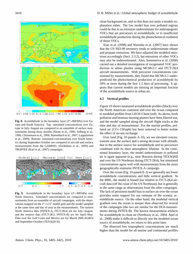
4.1 Continental boundary layer

Figure 8 compares simulated boundary layer (P>800 hPa)concentrations over Europe during July-August and overtropical South America during September-October to sur-face and airborne measurements collected during thosetimes (Slemr et al., 1996; Solberg et al., 1996; Christensenet al., 2000; Bartenbach et al., 2007; Karl et al., 2007;Eerdekens et al., 2009; Lappalainen et al., 2009). The modelcaptures the large-scale features and gradients seen in themeasurements, which include remote, rural, polluted, andforested sites and span 94◦ of latitude. There does not ap-pear to be a persistent bias in the model relative to thesecontinental boundary-layer datasets. The model is biased

low relative to the two Italian datasets, which are affectedby local anthropogenic sources. As we will see, this model-measurement discrepancy is also present over polluted areasin North America.

There have been a number of recent aircraft campaignsover North America, allowing a more detailed model eval-uation for that region. Figure 9 shows boundary layeracetaldehyde measurements during ITCT-2K2 (Parrish etal., 2004), ITCT-2K4 (Fehsenfeld et al., 2006), INTEX-A(Singh et al., 2006), INTEX-B (Singh et al., 2009), MI-LAGRO (Molina et al., 2010), and TEXAQS-II (Parrishet al., 2009) mapped onto the model grid, compared tomodel results sampled along the flight tracks at the timeof measurement. Biomass burning plumes (diagnosed byCH3CN>225 ppt or HCN>500 ppt) and fresh pollutionplumes (NO2>4 ppb or NOx:NOy>0.4) have been removedprior to gridding since they are not captured at the 2◦

×2.5◦

model resolution.

Observed concentrations in Fig. 9 are similar to those sim-ulated by GEOS-Chem, except over and downwind of pol-luted regions (US Northeast, Mexico City, southern Califor-nia) where a low model bias is evident. The discrepancy isunlikely to reflect an underestimate of direct urban/industrialemissions: this acetaldehyde source is small in the model(<2% of secondary production), and well-constrained by ob-served emission ratios relative to CO as discussed earlier.The problem appears specific to polluted areas, which ar-gues against a sink (i.e., OH) overestimate as the main ex-planation. Also, the fact that the predominant sources aswell as sinks of acetaldehyde are photochemical weakensthe sensitivity to model OH. The measurement artifacts men-tioned in Sect. 1 have been shown to be most significant in



Fig. 8. Acetaldehyde in the boundary layer (P>800 hPa) over Eu-rope and South America. Top: simulated concentrations over Eu-rope in July–August are compared to an ensemble of surface mea-surements during those months (Slemr et al., 1996; Solberg et al.,1996; Christensen et al., 2000; Bartenbach et al., 2007; Lappalainenet al., 2009). Bottom: simulated concentrations over South Amer-ica during September-October are compared to aircraft and surfacemeasurements from the GABRIEL (Eerdekens et al., 2009) andTROFFEE (Karl et al., 2007) campaigns.

Fig. 9. Acetaldehyde in the boundary layer (P>800 hPa) overNorth America. Simulated concentrations are compared to mea-surements from an ensemble of aircraft campaigns, with the obser-vations mapped on the 2◦

×2.5◦ model grid and the model sampledat the same time and day of year as the measurements. The easternNorth America data (INTEX-A, ITCT-2K4) are for July–August,and the western data (ITCT-2K2, INTEX-B) are for April–May.Data over the Gulf Coast and Mexico are for March (MILAGRO)and September-October (TEXAQS-II).

clean background air, and so this does not seem a tenable ex-planation either. The low model bias over polluted regionscould be due to an emission underestimate for anthropogenicVOCs that are precursors of acetaldehyde, or to insufficientacetaldehyde production during the photochemical oxidationof those VOCs.

Xiao et al. (2008) and Warneke et al. (2007) have shownthat the US NEI-99 inventory tends to underestimate ethaneand propane emissions. We have adjusted the modeled emis-sions accordingly (Sect. 2.3.2), but emissions of other VOCsmay also be underestimated. Also, Sommariva et al. (2008)carried out a detailed investigation of oxygenated VOC pro-duction in urban plumes using MCMv3.1 and ITCT-2K4aircraft measurements. With precursor concentrations con-strained by measurements, they found that MCMv3.1 under-predicted the photochemical production of acetaldehyde by50% or more during the first 1-2 days of processing. It ap-pears that current models are missing an important fractionof the acetaldehyde source in urban air.

4.2 Vertical profiles

Figure 10 shows measured acetaldehyde profiles (black) overthe North American continent and over the ocean comparedto modeled profiles from GEOS-Chem (red). As above, freshpollution and biomass burning plumes have been filtered out,and the model sampled along the aircraft flight tracks at thetime and day of measurement. For the marine profiles, pol-luted air (CO>150 ppb) has been removed to better isolatethe effect of air-sea exchange.

Over land (Fig. 10 panels A–D), we see elevated concen-trations near the surface and a strong decrease with altitude,due to the surface source for acetaldehyde and its precursorscombined with its short atmospheric lifetime. In the conti-nental boundary layer, the model underestimate in pollutedair is again apparent (e.g., near Houston during TEXAQSIIand over the US Northeast during ITCT-2K4), but simulatedconcentrations agree well with measurements from the moregeographically extensive INTEX-A campaign.

Over the ocean (Fig. 10 panels E–I) we generally see loweracetaldehyde concentrations and little vertical gradient. Inthe MBL, the model is biased low relative to ITCT-2K4 air-craft data (off the coast of the US Northeast), but is generallyin the same range as observations from the other campaigns.The lack of persistent model bias in surface air over the oceanprovides some support for our estimate of the oceanic ac-etaldehyde source. On the other hand, the modeled verticalgradient over the ocean is steeper than observed for severalof the campaigns (the two are similar for the DC8 measure-ments during INTEX-B). The known measurement artifactsfor acetaldehyde in clean air (Northway et al., 2004; Apel etal., 2008) make it difficult to directly test the modeled oceansource of acetaldehyde; we return to this point later.

The observed free tropospheric concentrations are muchhigher than the model for all marine and continental profiles



Fig. 10. Vertical profiles of acetaldehyde mixing ratio over theNorth American continent(A–D) and over the ocean(E–I). Air-craft measurements are shown in black with the error bars indicat-ing twice the standard error around the mean for each altitude bin.Red lines show the GEOS-Chem simulated profiles with the modelsampled at the same time and day of year as the observations. Notethe differing x-axis scales for the land and ocean profiles. See textfor details.

in Fig. 10. This problem was noted previously over the Pa-cific and North America (Staudt et al., 2003; Singh et al.,2004; Kwan et al., 2006), but those earlier comparisons werebased on a less thorough description of acetaldehyde sourcesand chemistry than presented in this paper. We see here thatthe issue persists with the improved simulation, and points to

Fig. 11. Vertical profiles of PAN:NOx ratio over the North Ameri-can continent(A–D) and over the ocean(E–I). Colors as in Fig. 10.See text for details.

a general discrepancy between the high measured acetalde-hyde concentrations in the free troposphere and present un-derstanding of its sources and atmospheric lifetime.

In the following section we evaluate the acetaldehyde sim-ulation indirectly in terms of consistency with measuredPAN and NOx. Hudman et al. (2007) found the verticalconcentration profiles for NOx and PAN to be individuallywell-simulated by GEOS-Chem compared to INTEX-A andITCT-2K4 measurements, after accounting for recent NorthAmerican emission reductions and a more realistic lightning



source. We focus here on PAN:NOx ratio comparisons in thefree troposphere and over the ocean, where the low acetalde-hyde levels (and possible measurement artifacts) make directcomparison of simulated and observed acetaldehyde concen-trations more uncertain.

4.3 PAN:NOx ratio

Since acetaldehyde, PAN, and NOx are related by well-defined chemistry, measured PAN and NOx concentrationsprovide an additional constraint with which to test the model.Any severe model bias for acetaldehyde should also manifestas a corresponding bias in the simulated PAN:NOx ratio.

Figure 11 compares vertical profiles of measured andsimulated PAN:NOx ratios for the same aircraft campaignsshown in Fig. 10. The methods used to measure thesespecies have been previously published and are summarizedby Raper et al. (2001) for PEM-TB, Singh et al. (2006) forINTEX-A, Fehsenfeld et al. (2006) for ITCT-2K4, Singh etal. (2009) for INTEX-B (DC8 aircraft), Parrish et al. (2009)for TEXAQS-II, and by Slusher et al. (2004) and Weinheimeret al. (1993) for INTEX-B (C130 aircraft). In all cases freshpollution and biomass burning plumes have been filtered outas above.

In contrast to the persistent and severe model underesti-mate of acetaldehyde concentrations relative to the free tro-pospheric measurements, we see that the PAN:NOx ratio isrelatively well-simulated. There are cases where the mea-sured ratio is higher than the model in the free troposphere(e.g., C130 data from INTEX-B), which would be consis-tent with a model underestimate of acetaldehyde. However,taken together, the PAN:NOx comparisons provide no cor-roboration for a large-scale missing source of acetaldehydein the free troposphere. A model sensitivity run in which weimposed a minimum acetaldehyde concentration of 100 pptthroughout the troposphere (an approximate lower boundbased on the average profiles in Fig. 10) resulted in unre-alistically high simulated PAN:NOx ratios: up to 5× higherthan observed.

In surface air over the ocean, the modeled PAN:NOx ratiosagree well with the measurements (Fig. 11). We estimatedthe ocean acetaldehyde source using a conservative assump-tion for its OML lifetime based on available data (Mopperand Kieber, 1991; Zhou and Mopper, 1997), leading to acomputed net ocean source of 57 Tg a−1. A longer assumedOML lifetime would result in a larger ocean source in themodel, which would agree better with the previous estimateof 125 Tg a−1 (Singh et al., 2004). However, a sensitivity runwith 125 Tg a−1 net oceanic emission produced PAN:NOxvertical gradients over the ocean less steep than observed,an overestimate of atmospheric acetaldehyde in the marineboundary layer compared to most of the airborne datasets,and higher acetaldehyde concentrations in the surface oceanthan seems tenable based on the range of observations (Mop-per and Kieber, 1991; Zhou and Mopper, 1997). We con-

clude that the balance of evidence argues against a signifi-cantly larger ocean source than used here.

5 Role of ethanol as acetaldehyde source

Ethanol is receiving attention as a renewable fuel with thepotential to reduce our reliance on fossil fuels and mitigateglobal warming. Analyses to date indicate that a transitionto ethanol fuels could cause significant air quality penaltiesor benefits, depending on how the ethanol is produced (Hillet al., 2006; Jacobson, 2007; Hill et al., 2009): in mone-tary terms, health impacts may outweigh greenhouse gas im-pacts. A study by Jacobson (2007) predicts that a switchto E85 ethanol fuel (85% ethanol fuel, 15% gasoline) in theUS would increase air pollution-related mortality, hospital-ization, and asthma relative to 100% gasoline. Projected airquality impacts of ethanol fuel use are closely tied to the as-sociated increase in acetaldehyde levels, from direct emis-sions and from photochemical oxidation of unburned ethanol(65–75% of organic gas emissions from E85 automobilesconsist of unburned ethanol itself; Black, 1991; Jacobson,2007).

Actual air pollution impacts of ethanol use will depend onthe ethanol and acetaldehyde increases relative to their exist-ing sources. We have provided here the first detailed assess-ment of existing sources for these compounds, totaling 25and 213 Tg a−1 globally. Jacobson (2007) estimates that con-verting the entire US vehicle fleet to E85 would increase ac-etaldehyde emissions by 0.14 Tg a−1 and ethanol emissionsby 2.1 Tg a−1 (considering tailpipe emissions only). Thesetwo compounds made up 76% by mass of the total projectednon-methane VOC emission increase, and 80% of the in-crease for potential acetaldehyde precursors (excluding C1compounds, unreactive compounds, and ethene). Account-ing for a 95% acetaldehyde yield from ethanol oxidation anda 23% depositional sink for ethanol (see above) this trans-lates to an approximate total acetaldehyde source increase of1.6 Tg a−1 for the US.

By comparison, we estimate the current US ethanol sourceat 1.3 Tg a−1, including 74% from biogenic emissions. Weestimate the current US acetaldehyde source at 7.8 Tg a−1,including direct emissions and secondary production but ex-cluding the ocean source. Here we consider only photo-chemical production occurring over the US; a conservativeassumption since VOC oxidation continues as air moves off-shore. We conclude that the projected increase in ethanolemissions for a US transition to E85 is comparable to the ex-isting US ethanol source (2.1 versus 1.3 Tg a−1), and that theassociated acetaldehyde source increase is equivalent to only21% of the current US acetaldehyde source. Studies inves-tigating how ethanol fuel use will affect air quality need toadequately account for these existing sources.



6 Key uncertainties and outstanding issues

In this section we examine the main sources of uncertainty inthe model evaluation and identify observational needs for re-fining the acetaldehyde source and sink estimates presentedhere. The acetaldehyde lifetime in the OML is a key param-eter for estimating the ocean source. Published estimates im-ply values between 0.3–12 h, but with no information on howit might vary in space and time (Mopper and Kieber, 1991;Zhou and Mopper, 1997). As a result, our computed oceansource carries significant uncertainty. Atmospheric measure-ments of acetaldehyde and PAN:NOx provide some supportfor our estimate of the sea-to-air flux and bounds on its mag-nitude, but additional measurements of acetaldehyde and itsturnover rates in the OML as well as air-sea flux would bevaluable constraints.

Another area of uncertainty is the source rate of precur-sor VOCs. Bottom-up uncertainties in VOC emissions canbe large (Xiao et al., 2008). Also, for simple precursorssuch as ethane and propene the time-dependent acetaldehydeyield is well known, but uncertainties are higher for morecomplex compounds including isoprene. Measurements ofacetaldehyde itself provide an integrating constraint on theproduct of precursor emissions and acetaldehyde yield. Wehave shown here that our acetaldehyde simulation capturesthe large-scale patterns and gradients in surface air observa-tions, but is biased low in polluted air. In contrast, there wasno model bias evident for formaldehyde concentrations rela-tive to aircraft measurements over the eastern US (Millet etal., 2006).

Biogenic emissions from terrestrial plants do not representa dominant term in the overall acetaldehyde budget, but thebottom-up uncertainty in this source is probably at least 50%based on the range of observed canopy-scale emission rates(see Supplemental Information). Simulated acetaldehydeconcentrations over the US Southeast and over the Amazonare generally similar to available aircraft and surface mea-surements, which lends support to the MEGANv2.1 emis-sions. Ethanol measurements are much sparser and more areneeded to better constrain its present-day budget and impor-tance as an acetaldehyde source. More information is alsoneeded to better parameterize the effect of soil moisture onemissions for both compounds.

Other potential sources of error in the acetaldehyde simu-lation include boundary layer venting and model OH. Pre-vious work with GEOS-Chem argues against a persistentmodel bias in the former (Millet et al., 2006; Xiao et al.,2007; Hudman et al., 2008). The error in mean OH is esti-mated at±10% for GEOS-Chem (Xiao et al., 2008), and inany case acetaldehyde is buffered to a degree since it is bothproduced and destroyed photochemically.

7 Conclusions

We used a global 3-D chemical transport model (GEOS-Chem) together with an ensemble of surface, airborne, andsatellite observations to carry out the first detailed analy-sis of the global acetaldehyde budget. We carried out ex-tensive updates to the GEOS-Chem chemical mechanism tomore accurately represent the production of acetaldehydefrom VOC oxidation, and the resulting chemical yields ofacetaldehyde are in general agreement with those from theMaster Chemical Mechanism (MCMv3.1). The dominantglobal acetaldehyde source in the model is photochemical(128 Tg a−1), most importantly from oxidation of alkanes,alkenes, ethanol, and isoprene. This is a factor of 4 largerthan the previous estimate (30 Tg a−1; Singh et al., 2004);the present work uses a more comprehensive and up-to-datetreatment of precursor emissions and their oxidation path-ways.

Monthly distributions of colored dissolved organic matter(CDOM) in the world’s oceans derived from satellite oceancolor observations allow us to estimate the oceanic sourceof acetaldehyde, based on published yields of acetaldehydefrom CDOM photodegradation (Kieber et al., 1990). Thisis an important step forward as the first calculation of theacetaldehyde sea-to-air flux that is tied to actual produc-tion rates in the ocean mixed layer (OML) as constrainedby observations. The resulting net global sea-to-air flux is57 Tg a−1, the second largest source term in the model buta factor of two smaller than the atmospheric source fromVOC oxidation. It is also a factor of two smaller than theprevious estimate of Singh et al. (2004), which was basedon atmospheric measurements over the Pacific Ocean. Ourrepresentation of the ocean source yields predicted acetalde-hyde concentrations over the ocean surface that are simi-lar to aircraft measurements; however, the modeled verticalgradient over the ocean is too steep relative to the observa-tions in several cases. Quantitative evaluation of the mod-eled ocean source against atmospheric acetaldehyde obser-vations is complicated by known measurement artifacts inclean air. Simulated PAN:NOx ratios agree well with ob-servations over the ocean which provides some support forthe modeled ocean source; however, more measurements areneeded to reduce its uncertainty.

Terrestrial sources of acetaldehyde in the model include23 Tg a−1 from vegetation and 3 Tg a−1 from biomass burn-ing. Direct anthropogenic emissions (including biofuel) arewell-constrained by measured emission ratios relative to COand amount to 2 Tg a−1 globally, 1% of the total source. Re-action with OH is the main acetaldehyde sink, accounting for88% of the total loss in the model. With photolysis (11%) andwet + dry deposition (<2%), the overall atmospheric lifetimefor acetaldehyde in the model is 0.8 days.

Simulated acetaldehyde mixing ratios generally agree wellwith aircraft and surface measurements in the continentalboundary layer, capturing broad patterns of concentration



and variability over North America, Europe, and the Ama-zon. There is no evidence of a persistent bias that would sug-gest a significant error in the primary and secondary terres-trial sources in the model. An exception is the low bias com-pared to aircraft measurements in polluted air, which must bedue to an underestimate of anthropogenic hydrocarbon emis-sions or of the associated acetaldehyde yield. Current modelsappear to be missing an important fraction of the acetalde-hyde source in polluted air.

We see a severe model-measurement discrepancy in thefree troposphere. For all of the aircraft campaigns exam-ined here, the observed acetaldehyde levels are substantiallyhigher than predicted by GEOS-Chem. The average freetropospheric bias ranges from a factor of 2–30, dependingon location and altitude. On the other hand, we find thatthe corresponding PAN:NOx ratios are well-simulated by themodel. This is an apparent contradiction based on present un-derstanding of acetaldehyde and PAN chemistry, since suchelevated acetaldehyde concentrations should also manifest ashigh PAN:NOx ratios compared to the model. We concludethat there is no strong evidence for a large missing acetalde-hyde source in the free troposphere.

Our work lays the groundwork for an improved assess-ment of the potential effects of ethanol fuel on air quality,since in the atmosphere ethanol is oxidized to acetaldehydenearly quantitatively. We find that current US acetaldehydesources (7.8 Tg a−1) are nearly 5× greater than the increasepredicted for a full vehicle fleet transition to ethanol fuel(1.6 Tg a−1; Jacobson, 2007). Current ethanol sources areless well constrained but appear to be predominantly bio-genic. We estimate current US emission at 1.3 Tg a−1, com-pared to an expected increase of 2.1 Tg a−1 for a transition toethanol fuel.

Acknowledgements.We gratefully acknowledge the science teamsfor the GABRIEL, INTEX-A, INTEX-B, ITCT-2K2, ITCT-2K4,MILAGRO, PEM-TB, TEXAQS-II, and TROFFEE aircraftexperiments. Particular thanks go to B. Brune, X. Ren, J. Mao,T. Ryerson, G. Huey, A. Weinheimer, and R. Cohen for the useof their airborne NO and NO2 measurements. MPB and PIPacknowledge funding from NERC (grant NE/D001471).

Edited by: P. Monks

References

Altshuller, A. P.: Chemical reactions and transport of alkanes andtheir products in the troposphere, J. Atmos. Chem., 12, 19–61,1991a.

Altshuller, A. P.: Estimating product yields of carbon-containingproducts from the atmospheric photooxidation of ambient airalkenes, J. Atmos. Chem., 13, 131–154, 1991b.

Andreae, M. O. and Merlet, P.: Emission of trace gases and aerosolsfrom biomass burning, Global Biogeochem. Cy., 15, 955–966,2001.

Apel, E. C., Hills, A. J., Lueb, R., Zindel, S., Eisele, S., andRiemer, D. D.: A fast-GC/MS system to measure C-2 to C-4carbonyls and methanol aboard aircraft, J. Geophys. Res., 108,8794, doi:10.1029/2002JD003199, 2003.

Apel, E. C., Brauers, T., Koppmann, R., Bandowe, B., Bossmeyer,J., Holzke, C., Tillmann, R., Wahner, A., Wegener, R., Brun-ner, A., Jocher, M., Ruuskanen, T., Spirig, C., Steigner, D.,Steinbrecher, R., Alvarez, E. G., Muller, K., Burrows, J. P.,Schade, G., Solomon, S. J., Ladstatter-Weissenmayer, A., Sim-monds, P., Young, D., Hopkins, J. R., Lewis, A. C., Legreid,G., Reimann, S., Hansel, A., Wisthaler, A., Blake, R. S., El-lis, A. M., Monks, P. S., and Wyche, K. P.: Intercomparisonof oxygenated volatile organic compound measurements at theSAPHIR atmosphere simulation chamber, J. Geophys. Res., 113,D20307, doi:10.1029/2008JD009865, 2008.

Atkinson, R., Baulch, D. L., Cox, R. A., Crowley, J. N., Hamp-son, R. F., Hynes, R. G., Jenkin, M. E., Rossi, M. J., and Troe, J.:Evaluated kinetic and photochemical data for atmospheric chem-istry: Volume II – gas phase reactions of organic species, Atmos.Chem. Phys., 6, 3625–4055, 2006,http://www.atmos-chem-phys.net/6/3625/2006/.

Ban-Weiss, G. A., McLaughlin, J. P., Harley, R. A., Kean, A. J.,Grosjean, E., and Grosjean, D.: Carbonyl and nitrogen diox-ide emissions from gasoline- and diesel-powered motor vehicles,Environ. Sci. Technol., 42, 3944–3950, 2008.

Bartenbach, S., Williams, J., Plass-Dulmer, C., Berresheim, H.,and Lelieveld, J.: In-situ measurement of reactive hydrocar-bons at Hohenpeissenberg with comprehensive two-dimensionalgas chromatography (GC× GC-FID): use in estimating HO andNO3, Atmos. Chem. Phys., 7, 1–14, 2007,http://www.atmos-chem-phys.net/7/1/2007/.

Bey, I., Jacob, D. J., Yantosca, R. M., Logan, J. A., Field, B. D.,Fiore, A. M., Li, Q. B., Liu, H. G. Y., Mickley, L. J., and Schultz,M. G.: Global modeling of tropospheric chemistry with assim-ilated meteorology: Model description and evaluation, J. Geo-phys. Res., 106, 23073–23095, 2001.

Black, F.: An overview of the technical implications of methanoland ethanol as highway motor vehicle fuels, EPA/600/D-91/239,US EPA, Washington DC, USA, 1991.

Bloss, C., Wagner, V., Jenkin, M. E., Volkamer, R., Bloss, W. J.,Lee, J. D., Heard, D. E., Wirtz, K., Martin-Reviejo, M., Rea,G., Wenger, J. C., and Pilling, M. J.: Development of a detailedchemical mechanism (MCMv3.1) for the atmospheric oxidationof aromatic hydrocarbons, Atmos. Chem. Phys., 5, 641–664,2005,http://www.atmos-chem-phys.net/5/641/2005/.

Christensen, C. S., Skov, H., Nielsen, T., and Lohse, C.: Temporalvariation of carbonyl compound concentrations at a semi-ruralsite in Denmark, Atmos. Environ., 34, 287–296, 2000.

Christian, T. J., Kleiss, B., Yokelson, R. J., Holzinger, R., Crutzen,P. J., Hao, W. M., Saharjo, B. H., and Ward, D. E.: Comprehen-sive laboratory measurements of biomass-burning emissions: 1.Emissions from Indonesian, African, and other fuels, J. Geophys.Res., 108, 4719, doi:10.1029/2003JD003704, 2003.

Cojocariu, C., Kreuzwieser, J., and Rennenberg, H.: Correlationof short-chained carbonyls emitted from Picea abies with phys-iological and environmental parameters, New Phytologist, 162,717–727, 2004.

Cojocariu, C., Escher, P., Haberle, K. H., Matyssek, R., Rennen-berg, H., and Kreuzwieser, J.: The effect of ozone on the emis-


http://www.atmos-chem-phys.net/6/3625/2006/




sion of carbonyls from leaves of adult Fagus sylvatica, Plant CellEnviron., 28, 603–611, 2005.

Colomb, A., Gros, V., Alvain, S., Sarda-Esteve, R., Bonsang, B.,Moulin, C., Klupfel, T., and Williams, J.: Variation of atmo-spheric volatile organic compounds over the Southern IndianOcean (30–49 degrees S), Environ. Chem., 6, 70–82, 2009.

Custer, T. and Schade, G.: Methanol and acetaldehyde fluxes overryegrass, Tellus B – Chem. Phys. Meteorol., 59, 673–684, 2007.

de Gouw, J. and Warneke, C.: Measurements of volatile or-ganic compounds in the earths atmosphere using proton-transfer-reaction mass spectrometry, Mass Spectrom. Rev., 26, 223–257,2007.

de Gouw, J. A., Howard, C. J., Custer, T. G., and Fall, R.: Emis-sions of volatile organic compounds from cut grass and cloverare enhanced during the drying process, Geophys. Res. Lett., 26,811–814, 1999.

de Gouw, J. A., Howard, C. J., Custer, T. G., Baker, B. M., andFall, R.: Proton-transfer chemical-ionization mass spectrome-try allows real-time analysis of volatile organic compounds re-leased from cutting and drying of crops, Environ. Sci. Technol.,34, 2640–2648, 2000.

de Gouw, J. A., Middlebrook, A. M., Warneke, C., Goldan, P.D., Kuster, W. C., Roberts, J. M., Fehsenfeld, F. C., Worsnop,D. R., Canagaratna, M. R., Pszenny, A. A. P., Keene, W. C.,Marchewka, M., Bertman, S. B., and Bates, T. S.: Budget of or-ganic carbon in a polluted atmosphere: Results from the NewEngland Air Quality Study in 2002, J. Geophys. Res., 110,D16305, doi:10.1029/2004JD005623, 2005.

de Gouw, J. A., Welsh-Bon, D., Warneke, C., Kuster, W. C., Alexan-der, L., Baker, A. K., Beyersdorf, A. J., Blake, D. R., Cana-garatna, M., Celada, A. T., Huey, L. G., Junkermann, W., Onasch,T. B., Salcido, A., Sjostedt, S. J., Sullivan, A. P., Tanner, D.J., Vargas, O., Weber, R. J., Worsnop, D. R., Yu, X. Y., andZaveri, R.: Emission and chemistry of organic carbon in thegas and aerosol phase at a sub-urban site near Mexico City inMarch 2006 during the MILAGRO study, Atmos. Chem. Phys.,9, 3425–3442, 2009,http://www.atmos-chem-phys.net/9/3425/2009/.

Duncan, B. N., Logan, J. A., Bey, I., Megretskaia, I. A., Yan-tosca, R. M., Novelli, P. C., Jones, N. B., and Rinsland, C. P.:Global budget of CO, 1988-1997: Source estimates and val-idation with a global model, J. Geophys. Res., 112, D22301,doi:10.1029/2007JD008459, 2007.

Eerdekens, G., Ganzeveld, L., de Arellano, J. V. G., Klupfel, T.,Sinha, V., Yassaa, N., Williams, J., Harder, H., Kubistin, D., Mar-tinez, M., and Lelieveld, J.: Flux estimates of isoprene, methanoland acetone from airborne PTR-MS measurements over the trop-ical rainforest during the GABRIEL 2005 campaign, Atmos.Chem. Phys., 9, 4207–4227, 2009,http://www.atmos-chem-phys.net/9/4207/2009/.

Emmerson, K. M. and Evans, M. J.: Comparison of troposphericgas-phase chemistry schemes for use within global models, At-mos. Chem. Phys., 9, 1831–1845, 2009,http://www.atmos-chem-phys.net/9/1831/2009/.

EPA: Chemical summary for acetaldehyde, EPA 749-F-94-003a,Office of Pollution Prevention and Toxics, 1994.

EPA NEI 2002 inventory:http://www.epa.gov/oar/data/, last ac-cess: 2007.

Fall, R.: Abundant oxygenates in the atmosphere: A biochemical

perspective, Chem. Rev., 103, 4941–4951, 2003.Fehsenfeld, F. C., Ancellet, G., Bates, T. S., Goldstein, A. H., Hard-

esty, R. M., Honrath, R., Law, K. S., Lewis, A. C., Leaitch, R.,McKeen, S., Meagher, J., Parrish, D. D., Pszenny, A. A. P., Rus-sell, P. B., Schlager, H., Seinfeld, J., Talbot, R., and Zbinden, R.:International Consortium for Atmospheric Research on Trans-port and Transformation (ICARTT): North America to Europe –Overview of the 2004 summer field study, J. Geophys. Res., 111,D23S01, doi:10.1029/2006JD007829, 2006.

Filella, I., Penuelas, J., and Seco, R.: Short-chained oxygenatedVOC emissions in Pinus halepensis in response to changes inwater availability, Acta Physiol. Plant., 31, 311–318, 2009.

GMAO: File Specification for GEOS-5 DAS Gridded Output, ver-sion 6.4, http://gmao.gsfc.nasa.gov/operations/, NASA GlobalModeling and Assimilation Office (GMAO), 2008.

Grabmer, W., Kreuzwieser, J., Wisthaler, A., Cojocariu, C., Graus,M., Rennenberg, H., Steigner, D., Steinbrecher, R., and Hansel,A.: VOC emissions from Norway spruce (Picea abies L. [Karst])twigs in the field – Results of a dynamic enclosure study, Atmos.Environ., 40, S128–S137, 2006.

Granier, C., Lamarque, J. F., Mieville, A., Muller, J. F., Olivier,J., Orlando, J., Peters, J., Petron, G., Tyndall, G., and Wallens,S.: POET, a database of surface emissions of ozone precursors,http://www.aero.jussieu.fr/projet/ACCENT/POET.php, 2005.

Greenberg, J. P., Friedli, H., Guenther, A. B., Hanson, D., Harley, P.,and Karl, T.: Volatile organic emissions from the distillation andpyrolysis of vegetation, Atmos. Chem. Phys., 6, 81–91, 2006,http://www.atmos-chem-phys.net/6/81/2006/.

Grosjean, D., Williams, E. L., and Grosjean, E.: Atmosphericchemistry of isoprene and of its carbonyl products, Environ. Sci.Technol., 27, 830–840, 1993.

Guenther, A., Baugh, B., Brasseur, G., Greenberg, J., Harley, P.,Klinger, L., Serca, D., and Vierling, L.: Isoprene emission es-timates and uncertainties for the Central African EXPRESSOstudy domain, J. Geophys. Res., 104, 30625–30639, 1999.

Guenther, A., Karl, T., Harley, P., Wiedinmyer, C., Palmer, P. I.,and Geron, C.: Estimates of global terrestrial isoprene emissionsusing MEGAN (Model of Emissions of Gases and Aerosols fromNature), Atmos. Chem. Phys., 6, 3181–3210, 2006,http://www.atmos-chem-phys.net/6/3181/2006/.

Hill, J., Nelson, E., Tilman, D., Polasky, S., and Tiffany, D.:Environmental, economic, and energetic costs and benefits ofbiodiesel and ethanol biofuels, P. Natl. Acad. Sci. USA, 103,11206–11210, 2006.

Hill, J., Polasky, S., Nelson, E., Tilman, D., Huo, H., Ludwig, L.,Neumann, J., Zheng, H. C., and Bonta, D.: Climate change andhealth costs of air emissions from biofuels and gasoline, P. Natl.Acad. Sci. USA, 106, 2077–2082, 2009.

Holzinger, R., Warneke, C., Hansel, A., Jordan, A., Lindinger, W.,Scharffe, D.H., Schade, G., and Crutzen, P.J.: Biomass burn-ing as a source of formaldehyde, acetaldehyde, methanol, ace-tone, acetonitrile, and hydrogen cyanide, Geophys. Res. Lett.,26, 1161-1164, 1999.

Holzinger, R., Sandoval-Soto, L., Rottenberger, S., Crutzen, P. J.,and Kesselmeier, J.: Emissions of volatile organic compoundsfrom Quercus ilex L. measured by Proton Transfer ReactionMass Spectrometry under different environmental conditions, J.Geophys. Res., 105, 20573–20579, 2000.

Hudman, R. C., Jacob, D. J., Turquety, S., Leibensperger, E. M.,





http://www.epa.gov/oar/data/

http://gmao.gsfc.nasa.gov/operations/

http://www.aero.jussieu.fr/projet/ACCENT/POET.php




Murray, L. T., Wu, S., Gilliland, A. B., Avery, M., Bertram, T.H., Brune, W., Cohen, R. C., Dibb, J. E., Flocke, F. M., Fried, A.,Holloway, J., Neuman, J. A., Orville, R., Perring, A., Ren, X.,Sachse, G. W., Singh, H. B., Swanson, A., and Wooldridge, P. J.:Surface and lightning sources of nitrogen oxides over the UnitedStates: Magnitudes, chemical evolution, and outflow, J. Geo-phys. Res., 112, D12S05, doi:10.1029/2006JD007912, 2007.

Hudman, R. C., Murray, L. T., Jacob, D. J., Millet, D. B., Tur-quety, S., Wu, S., Blake, D. R., Goldstein, A. H., Holloway,J., and Sachse, G. W.: Biogenic vs. anthropogenic sources ofCO over the United States, Geophys. Res. Lett., 35, L04801,doi:10.1029/2007GL032393, 2008.

Jacob, D. J., Field, B. D., Li, Q. B., Blake, D. R., de Gouw,J., Warneke, C., Hansel, A., Wisthaler, A., Singh, H. B.,and Guenther, A.: Global budget of methanol: Constraintsfrom atmospheric observations, J. Geophys. Res., 110, D08303,doi:10.1029/2004JD005172, 2005.

Jacobson, M. Z.: Effects of ethanol (E85) versus gasoline vehicleson cancer and mortality in the United States, Environ. Sci. Tech-nol., 41, 4150–4157, 2007.

Jardine, K., Harley, P., Karl, T., Guenther, A., Lerdau, M., and Mak,J. E.: Plant physiological and environmental controls over theexchange of acetaldehyde between forest canopies and the atmo-sphere, Biogeosciences, 5, 1559–1572, 2008,http://www.biogeosciences.net/5/1559/2008/.

Karl, T., Guenther, A., Jordan, A., Fall, R., and Lindinger, W.: Eddycovariance measurement of biogenic oxygenated VOC emissionsfrom hay harvesting, Atmos. Environ., 35, 491–495, 2001a.

Karl, T., Guenther, A., Lindinger, C., Jordan, A., Fall, R., andLindinger, W.: Eddy covariance measurements of oxygenatedvolatile organic compound fluxes from crop harvesting using aredesigned proton-transfer-reaction mass spectrometer, J. Geo-phys. Res., 106, 24157–24167, 2001b.

Karl, T., Curtis, A. J., Rosenstiel, T. N., Monson, R. K., and Fall, R.:Transient releases of acetaldehyde from tree leaves – products ofa pyruvate overflow mechanism?, Plant Cell Environ., 25, 1121–1131, 2002.

Karl, T., Guenther, A., Spirig, C., Hansel, A., and Fall, R.: Sea-sonal variation of biogenic VOC emissions above a mixed hard-wood forest in northern Michigan, Geophys. Res. Lett., 30, 2186,doi:10.1029/2003GL018432, 2003.

Karl, T., Potosnak, M., Guenther, A., Clark, D., Walker, J., Her-rick, J. D., and Geron, C.: Exchange processes of volatile organiccompounds above a tropical rain forest: Implications for model-ing tropospheric chemistry above dense vegetation, J. Geophys.Res., 109, D18306, doi:10.1029/2004JD004738, 2004.

Karl, T., Harley, P., Guenther, A., Rasmussen, R., Baker, B., Jar-dine, K., and Nemitz, E.: The bi-directional exchange of oxy-genated VOCs between a loblolly pine (Pinus taeda) plantationand the atmosphere, Atmos. Chem. Phys., 5, 3015–3031, 2005a,http://www.atmos-chem-phys.net/5/3015/2005/.

Karl, T., Harren, F., Warneke, C., de Gouw, J., Grayless, C., andFall, R.: Senescing grass crops as regional sources of reactivevolatile organic compounds, J. Geophys. Res., 110, D15302,doi:10.1029/2005JD005777, 2005b.

Karl, T. G., Christian, T. J., Yokelson, R. J., Artaxo, P., Hao, W.M., and Guenther, A.: The Tropical Forest and Fire EmissionsExperiment: method evaluation of volatile organic compoundemissions measured by PTR-MS, FTIR, and GC from tropical

biomass burning, Atmos. Chem. Phys., 7, 5883–5897, 2007,http://www.atmos-chem-phys.net/7/5883/2007/.

Kesselmeier, J.: Exchange of short-chain oxygenated volatile or-ganic compounds (VOCs) between plants and the atmosphere: Acompilation of field and laboratory studies, J. Atmos. Chem., 39,219–233, 2001.

Kieber, R. J., Zhou, X. L., and Mopper, K.: Formation of carbonylcompounds from UV-induced photodegradation of humic sub-stances in natural waters: Fate of riverine carbon in the sea, Lim-nol. Oceanogr., 35, 1503–1515, 1990.

Kimmerer, T. W. and Kozlowski, T. T.: Ethylene, ethane, acetalde-hyde, and ethanol production by plants under stress, Plant Phys-iol., 69, 840–847, 1982.

Kimmerer, T. W. and Macdonald, R. C.: Acetaldehyde and ethanolbiosynthesis in leaves of plants, Plant Physiol., 84, 1204–1209,1987.

Kirstine, W., Galbally, I., Ye, Y. R., and Hooper, M.: Emissions ofvolatile organic compounds (primarily oxygenated species) frompasture, J. Geophys. Res., 103, 10605–10619, 1998.

Kreuzwieser, J., Schnitzler, J. P., and Steinbrecher, R.: Biosynthesisof organic compounds emitted by plants, Plant Biol., 1, 149–159,1999.

Kreuzwieser, J., Kuhnemann, F., Martis, A., Rennenberg, H., andUrban, W.: Diurnal pattern of acetaldehyde emission by floodedpoplar trees, Physiologia Plantarum, 108, 79–86, 2000.

Kreuzwieser, J., Papadopoulou, E., and Rennenberg, H.: Interactionof flooding with carbon metabolism of forest trees, Plant Biol.,6, 299–306, 2004.

Kuhns, H., Knipping, E. M., and Vukovich, J. M.: Developmentof a United States-Mexico emissions inventory for the Big BendRegional Aerosol and Visibility Observational (BRAVO) Study,J. Air & Waste Manage. Assoc., 55, 677-692, 2005.

Kwan, A. J., Crounse, J. D., Clarke, A. D., Shinozuka, Y., An-derson, B. E., Crawford, J. H., Avery, M. A., McNaughton,C. S., Brune, W. H., Singh, H. B., and Wennberg, P. O.:On the flux of oxygenated volatile organic compounds fromorganic aerosol oxidation, Geophys. Res. Lett., 33, L15815,doi:10.1029/2006GL026144, 2006.

Lappalainen, H. K., Sevanto, S., Back, J., Ruuskanen, T. M., Ko-lari, P., Taipale, R., Rinne, J., Kulmala, M., and Hari, P.: Day-time concentrations of biogenic volatile organic compounds in aboreal forest canopy and their relation to environmental and bio-logical factors, Atmos. Chem. Phys., 9, 5447–5459, 2009,http://www.atmos-chem-phys.net/9/5447/2009/.

Lee, A., Goldstein, A. H., Kroll, J. H., Ng, N. L., Varut-bangkul, V., Flagan, R. C., and Seinfeld, J. H.: Gas-phaseproducts and secondary aerosol yields from the photooxida-tion of 16 different terpenes, J. Geophys. Res., 111, D17305,doi:10.1029/2006JD007050, 2006.

Madronich, S., and Calvert, J.G.: Permutation reactions of organicperoxy radicals in the troposphere, J. Geophys. Res., 95, 5697-5715, 1990.

Maritorena, S., Siegel, D. A., and Peterson, A. R.: Optimization ofa semianalytical ocean color model for global-scale applications,Appl. Opt., 41, 2705–2714, 2002.

Millet, D. B., Jacob, D. J., Turquety, S., Hudman, R. C., Wu, S.,Fried, A., Walega, J., Heikes, B. G., Blake, D. R., Singh, H.B., Anderson, B. E., and Clarke, A. D.: Formaldehyde distribu-tion over North America: Implications for satellite retrievals of


http://www.biogeosciences.net/5/1559/2008/





formaldehyde columns and isoprene emission, J. Geophys. Res.,111, D24S02, doi:10.1029/2005JD006853, 2006.

Millet, D. B., Jacob, D. J., Boersma, K. F., Fu, T. M., Kurosu, T.P., Chance, K., Heald, C. L., and Guenther, A.: Spatial distri-bution of isoprene emissions from North America derived fromformaldehyde column measurements by the OMI satellite sen-sor, J. Geophys. Res., 113, D02307, doi:10.1029/2007JD008950,2008a.

Millet, D. B., Jacob, D. J., Custer, T. G., Gouw, J. A. d., Goldstein,A. H., Karl, T., Singh, H. B., Sive, B. C., Talbot, R. W., Warneke,C., and Williams, J.: New constraints on terrestrial and oceanicsources of atmospheric methanol, Atmos. Chem. Phys., 8, 6887–6905, 2008b,http://www.atmos-chem-phys.net/8/6887/2008/.

Millet, D. B., Atlas, E. L., Blake, D. R., Blake, N. J., Diskin, G.S., Holloway, J. S., Meinardi, S., Ryerson, T. B., and Sachse, G.W.: Halocarbon emissions from the United States and Mexicoand their global warming potential, Environ. Sci. Technol., 43,1055–1060, 2009.

Molina, L. T., Madronich, S., Gaffney, J. S., Apel, E., Foy, B.d., Fast, J., Ferrare, R., Herndon, S., Jimenez, J. L., Lamb, B.,Osornio-Vargas, A. R., Russell, P., Schauer, J. J., Stevens, P. S.,and Zavala, M.: An overview of the MILAGRO 2006 campaign:Mexico City emissions and their transport and transformation,Atmos. Chem. Phys. Discuss., 10, 7819–7983, 2010,http://www.atmos-chem-phys-discuss.net/10/7819/2010/.

Montegut, C. D., Madec, G., Fischer, A. S., Lazar, A., and Iudicone,D.: Mixed layer depth over the global ocean: An examination ofprofile data and a profile-based climatology, J. Geophys. Res.-Ocean., 109, C12003, doi:10.1029/2004JC002378, 2004.

Mopper, K. and Kieber, D. J.: Distribution and biological turnoverof dissolved organic compounds in the water column of the BlackSea, Deep-Sea Res., 38, S1021–S1047, 1991.

Nelson, N. B., Siegel, D. A., and Michaels, A. F.: Seasonal dynam-ics of colored dissolved material in the Sargasso Sea, Deep-SeaRes. Pt. I, 45, 931–957, 1998.

Nelson, N. B., Siegel, D. A., Carlson, C. A., Swan, C., Smethie, W.M., and Khatiwala, S.: Hydrography of chromophoric dissolvedorganic matter in the North Atlantic, Deep-Sea Res. Pt. I, 54,710–731, 2007.

Northway, M. J., de Gouw, J. A., Fahey, D. W., Gao, R. S., Warneke,C., Roberts, J. M., and Flocke, F.: Evaluation of the role of het-erogeneous oxidation of alkenes in the detection of atmosphericacetaldehyde, Atmos. Environ., 38, 6017-6028, 2004.

Olivier, J., Peters, J., Granier, C., Petron, G., Muller, J. F., and Wal-lens, S.: Present and future surface emissions of atmosphericcompounds, POET report #2, EU project EVK2-1999-00011,2003.

Parrish, D. D., Kondo, Y., Cooper, O. R., Brock, C. A., Jaffe,D. A., Trainer, M., Ogawa, T., Hubler, G., and Fehsenfeld,F. C.: Intercontinental Transport and Chemical Transformation2002 (ITCT 2K2) and Pacific Exploration of Asian Continen-tal Emission (PEACE) experiments: An overview of the 2002winter and spring intensives, J. Geophys. Res., 109, D23S01,doi:10.1029/2004JD004980, 2004.

Parrish, D. D., Allen, D. T., Bates, T. S., Estes, M., Fehsenfeld, F.C., Feingold, G., Ferrare, R., Hardesty, R. M., Meagher, J. F.,Nielsen-Gammon, J. W., Pierce, R. B., Ryerson, T. B., Seinfeld,J. H., and Williams, E. J.: Overview of the Second Texas Air

Quality Study (TexAQS II) and the Gulf of Mexico AtmosphericComposition and Climate Study (GoMACCS), J. Geophys. Res.,114, D00F13, doi:10.1029/2009JD011842, 2009.

Paulson, S. E., Flagan, R. C., and Seinfeld, J. H.: Atmospheric pho-tooxidation of isoprene. Part II: The ozone-isoprene reaction, Int.J. Chem. Kin., 24, 103–125, 1992.

Randerson, J. T., Thompson, M. V., Conway, T. J., Fung, I. Y., andField, C. B.: The contribution of terrestrial sources and sinksto trends in the seasonal cycle of atmospheric carbon dioxide,Global Biogeochem. Cy., 11, 535–560, 1997.

Randerson, J. T., van der Werf, G. R., Giglio, L., Collatz, G. J.,and Kasibhatla, P. S.: Global Fire Emissions Database, Version 2(GFEDv2), Oak Ridge National Laboratory Distributed ActiveArchive Center (idoi:10.3334/ORNLDAAC/834), Oak Ridge,TN, USA, 2006.

Raper, J. L., Kleb, M. M., Jacob, D. J., Davis, D. D., Newell, R.E., Fuelberg, H. E., Bendura, R. J., Hoell, J. M., and McNeal,R. J.: Pacific Exploratory Mission in the tropical Pacific: PEM-Tropics B, March–April 1999, J. Geophys. Res., 106, 32401–32425, 2001.

Roberts, J. M.: The atmospheric chemistry of organic nitrates, At-mos. Environ., 24A, 243–287, 1990.

Rottenberger, S., Kuhn, U., Wolf, A., Schebeske, G., Oliva, S. T.,Tavares, T. M., and Kesselmeier, J.: Exchange of short-chainaldehydes between Amazonian vegetation and the atmosphere,Ecol. Appl., 14, S247–S262, 2004.

Rottenberger, S., Kuhn, U., Wolf, A., Schebeske, G., Oliva, S. T.,Tavares, T. M., and Kesselmeier, J.: Formaldehyde and acetalde-hyde exchange during leaf development of the Amazonian de-ciduous tree species Hymenaea courbaril, Atmos. Environ., 39,2275–2279, 2005.

Rottenberger, S., Kleiss, B., Kuhn, U., Wolf, A., Piedade, M. T. F.,Junk, W., and Kesselmeier, J.: The effect of flooding on the ex-change of the volatile C-2-compounds ethanol, acetaldehyde andacetic acid between leaves of Amazonian floodplain tree speciesand the atmosphere, Biogeosciences, 5, 1085–1100, 2008,http://www.biogeosciences.net/5/1085/2008/.

Sander, S. P., Friedl, R. R., Golden, D. M., Kurylo, M. J., Moortgat,G. K., Wine, P. H., Ravishankara, A. R., Kolb, C. E., Molina, M.J., Finlayson-Pitts, B. J., Huie, R. E., and Orkin, V. L.: Chemi-cal kinetics and photochemical data for use in atmospheric stud-ies: Evaluation number 15, JPL Publication 02-25, Jet Propul-sion Laboratory, Pasadena, USA, 2006.

Schade, G. W. and Goldstein, A. H.: Fluxes of oxygenated volatileorganic compounds from a ponderosa pine plantation, J. Geo-phys. Res., 106, 3111–3123, 2001.

Schade, G. W. and Goldstein, A. H.: Plant physiological in-fluences on the fluxes of oxygenated volatile organic com-pounds from ponderosa pine trees, J. Geophys. Res., 107, 4082,doi:10.1029/2001JD000532, 2002.

Schnitzler, J. P., Bauknecht, N., Bruggemann, N., Einig, W., Forkel,R., Hampp, R., Heiden, A. C., Heizmann, U., Hoffmann, T.,Holzke, C., Jaeger, L., Klauer, M., Komenda, M., Koppmann, R.,Kreuzwieser, J., Mayer, H., Rennenberg, H., Smiatek, G., Stein-brecher, R., Wildt, J., and Zimmer, W.: Emission of biogenicvolatile organic compounds: An overview of field, laboratoryand modelling studies performed during the ‘Tropospheric Re-search Program’ (TFS) 1997–2000, J. Atmos. Chem., 42, 159–177, 2002.



http://www.atmos-chem-phys-discuss.net/10/7819/2010/

http://www.biogeosciences.net/5/1085/2008/


Siegel, D. A., Maritorena, S., Nelson, N. B., Hansell, D. A., andLorenzi-Kayser, M.: Global distribution and dynamics of col-ored dissolved and detrital organic materials, J. Geophys. Res.-Ocean., 107, 3228, doi:10.1029/2001JC000965, 2002.

Siegel, D. A., Maritorena, S., Nelson, N. B., and Behrenfeld, M. J.:Independence and interdependencies among global ocean colorproperties: Reassessing the bio-optical assumption, J. Geophys.Res.-Ocean., 110, C07011, doi:10.1029/2004JC002527, 2005.

Singh, H., Chen, Y., Staudt, A., Jacob, D., Blake, D., Heikes, B.,and Snow, J.: Evidence from the Pacific troposphere for largeglobal sources of oxygenated organic compounds, Nature, 410,1078–1081, 2001.

Singh, H. B., Kanakidou, M., Crutzen, P. J., and Jacob, D. J.: Highconcentrations and photochemical fate of oxygenated hydrocar-bons in the global troposphere, Nature, 378, 50–54, 1995.

Singh, H. B., Tabazadeh, A., Evans, M. J., Field, B. D., Jacob,D. J., Sachse, G., Crawford, J. H., Shetter, R., and Brune, W.H.: Oxygenated volatile organic chemicals in the oceans: In-ferences and implications based on atmospheric observationsand air-sea exchange models, Geophys. Res. Lett., 30, 1862,doi:10.1029/2003GL017933, 2003.

Singh, H. B., Salas, L. J., Chatfield, R. B., Czech, E., Fried,A., Walega, J., Evans, M. J., Field, B. D., Jacob, D. J.,Blake, D., Heikes, B., Talbot, R., Sachse, G., Crawford, J.H., Avery, M. A., Sandholm, S., and Fuelberg, H.: Analy-sis of the atmospheric distribution, sources, and sinks of oxy-genated volatile organic chemicals based on measurements overthe Pacific during TRACE-P, J. Geophys. Res., 109, D15S07,doi:10.1029/2003JD003883, 2004.

Singh, H. B., Brune, W. H., Crawford, J. H., Jacob, D. J., and Rus-sell, P. B.: Overview of the summer 2004 intercontinental chem-ical transport experiment - North America (INTEX-A), J. Geo-phys. Res., 111, D24S01, doi:10.1029/2006JD007905, 2006.

Singh, H. B., Brune, W. H., Crawford, J. H., Flocke, F., and Jacob,D. J.: Chemistry and transport of pollution over the Gulf of Mex-ico and the Pacific: spring 2006 INTEX-B campaign overviewand first results, Atmos. Chem. Phys., 9, 2301–2318, 2009,http://www.atmos-chem-phys.net/9/2301/2009/.

Sinha, V., Williams, J., Meyerhofer, M., Riebesell, U., Paulino, A.I., and Larsen, A.: Air-sea fluxes of methanol, acetone, acetalde-hyde, isoprene and DMS from a Norwegian fjord following aphytoplankton bloom in a mesocosm experiment, Atmos. Chem.Phys., 7, 739–755, 2007,http://www.atmos-chem-phys.net/7/739/2007/.

Slemr, J., Junkermann, W., and VolzThomas, A.: Temporal varia-tions in formaldehyde, acetaldehyde and acetone and budget offormaldehyde at a rural site in southern Germany, Atmos. Envi-ron., 30, 3667–3676, 1996.

Slusher, D. L., Huey, L. G., Tanner, D. J., Flocke, F. M., andRoberts, J. M.: A thermal dissociation-chemical ionization massspectrometry (TD-CIMS) technique for the simultaneous mea-surement of peroxyacyl nitrates and dinitrogen pentoxide, J.Geophys. Res., 109, D19315, doi:10.1029/2004JD004670, 2004.

Solberg, S., Dye, C., Schmidbauer, N., Herzog, A., and Gehrig, R.:Carbonyls and nonmethane hydrocarbons at rural European sitesfrom the Mediterranean to the Arctic, J. Atmos. Chem., 25, 33–66, 1996.

Sommariva, R., de Gouw, J. A., Trainer, M., Atlas, E., Goldan, P.D., Kuster, W. C., Warneke, C., and Fehsenfeld, F. C.: Emis-

sions and photochemistry of oxygenated VOCs in urban plumesin the Northeastern United States, Atmos. Chem. Phys. Disc., 8,12371–12408, 2008.

Staudt, A. C., Jacob, D. J., Ravetta, F., Logan, J. A., Bachiochi,D., Krishnamurti, T. N., Sandholm, S., Ridley, B., Singh, H.B., and Talbot, B.: Sources and chemistry of nitrogen ox-ides over the tropical Pacific, J. Geophys. Res., 108, 8239,doi:10.1029/2002JD002139, 2003.

Swan, C. M., Siegel, D. A., Nelson, N. B., Carlson, C. A., and Nasir,E.: Biogeochemical and hydrographic controls on chromophoricdissolved organic matter distribution in the Pacific Ocean, Deep-Sea Res. Pt. I, 54, 710–731, 2009.

Taraborrelli, D., Lawrence, M. G., Butler, T. M., Sander, R., andLelieveld, J.: Mainz Isoprene Mechanism 2 (MIM2): an isopreneoxidation mechanism for regional and global atmospheric mod-elling, Atmos. Chem. Phys., 9, 2751–2777, 2009,http://www.atmos-chem-phys.net/9/2751/2009/.

Tyndall, G. S., Cox, R. A., Granier, C., Lesclaux, R., Moortgat,G. K., Pilling, M. J., Ravishankara, A. R., and Wallington, T.J.: Atmospheric chemistry of small organic peroxy radicals, J.Geophys. Res., 106, 12157–12182, 2001.

van der Werf, G. R., Randerson, J. T., Giglio, L., Collatz, G. J.,Kasibhatla, P. S., and Arellano, A. F.: Interannual variability inglobal biomass burning emissions from 1997 to 2004, Atmos.Chem. Phys., 6, 3423–3441, 2006,http://www.atmos-chem-phys.net/6/3423/2006/.

Vestreng, V. and Klein, H.: Emission data reported to UN-ECE/EMEP: Quality assurance and trend analysis & Presenta-tion of WebDab, MSC-W Status Report 2002, Norwegian Mete-orological Institute, Oslo, 2002.

Warneke, C., Karl, T., Judmaier, H., Hansel, A., Jordan, A.,Lindinger, W., and Crutzen, P. J.: Acetone, methanol, and otherpartially oxidized volatile organic emissions from dead plantmatter by abiological processes: Significance for atmosphericHOx chemistry, Global Biogeochem. Cy., 13, 9–17, 1999.

Warneke, C., Luxembourg, S. L., de Gouw, J. A., Rinne, H. J. I.,Guenther, A. B., and Fall, R.: Disjunct eddy covariance measure-ments of oxygenated volatile organic compounds fluxes from analfalfa field before and after cutting, J. Geophys. Res., 107, 4067,10.1029/2001JD000594, 2002.

Warneke, C., McKeen, S. A., de Gouw, J. A., Goldan, P. D.,Kuster, W. C., Holloway, J. S., Williams, E. J., Lerner, B. M.,Parrish, D. D., Trainer, M., Fehsenfeld, F. C., Kato, S., At-las, E. L., Baker, A., and Blake, D. R.: Determination of ur-ban volatile organic compound emission ratios and comparisonwith an emissions database, J. Geophys. Res., 112, D10S47,doi:10.1029/2006JD007930, 2007.

Weinheimer, A. J., Walega, J. G., Ridley, B. A., Sachse, G. W.,Anderson, B. E., and Collins, J. E.: Stratospheric NOy measure-ments on the NASA DC-8 during AASE-II, Geophys. Res. Lett.,20, 2563–2566, 1993.

Winters, A. J., Adams, M. A., Bleby, T. M., Rennenberg, H.,Steigner, D., Steinbrecher, R., and Kreuzwieser, J.: Emissions ofisoprene, monoterpene and short-chained carbonyl compoundsfrom Eucalyptus spp. in southern Australia, Atmos. Environ., 43,3035–3043, 2009.

Xiao, Y. P., Logan, J. A., Jacob, D. J., Hudman, R. C., Yantosca,R., and Blake, D. R.: Global budget of ethane and regionalconstraints on US sources, J. Geophys. Res., 113, D21306,







doi:10.1029/2007JD009415, 2008.Yang, W., Shabanov, N. V., Huang, D., Wang, W., Dickinson, R.

E., Nemani, R. R., Knyazikhin, Y., and Myneni, R. B.: Analysisof leaf area index products from combination of MODIS Terraand Aqua data, Remote Sensing of Environment, 104, 297–312,2006.

Yevich, R. and Logan, J. A.: An assessment of biofuel use and burn-ing of agricultural waste in the developing world, Global Bio-geochem. Cy., 17, 1095, doi:10.1029/2002GB001952, 2003.

Yokelson, R. J., Christian, T. J., Karl, T. G., and Guenther, A.:The tropical forest and fire emissions experiment: laboratory firemeasurements and synthesis of campaign data, Atmos. Chem.Phys., 8, 3509–3527, 2008,http://www.atmos-chem-phys.net/8/3509/2008/.

Zavala, M., Herndon, S. C., Wood, E. C., Jayne, J. T., Nelson, D.D., Trimborn, A. M., Dunlea, E., Knighton, W. B., Mendoza, A.,Allen, D. T., Kolb, C. E., Molina, M.J., and Molina, L. T.: Com-parison of emissions from on-road sources using a mobile lab-oratory under various driving and operational sampling modes,Atmos. Chem. Phys., 9, 1–14, 2009,http://www.atmos-chem-phys.net/9/1/2009/.

Zhang, J. F. and Smith, K. R.: Emissions of carbonyl compoundsfrom various cookstoves in China, Environ. Sci. Technol., 33,2311–2320, 1999.

Zhang, Q., Streets, D. G., Carmichael, G. R., He, K. B., Huo, H.,Kannari, A., Klimont, Z., Park, I. S., Reddy, S., Fu, J. S., Chen,D., Duan, L., Lei, Y., Wang, L. T., and Yao, Z. L.: Asian emis-sions in 2006 for the NASA INTEX-B mission, Atmos. Chem.Phys., 9, 5131–5153, 2009,http://www.atmos-chem-phys.net/9/5131/2009/.

Zhou, X. L. and Mopper, K.: Photochemical production of low-molecular-weight carbonyl compounds in seawater and surfacemicrolayer and their air-sea exchange, Mar. Chem., 56, 201–213,1997.





global atmospheric budget of acetaldehyde: 3-d model analysis … · facts by northway et al....

Documents