growth optimal portfolio selection strategies with transaction costs
TRANSCRIPT
8/9/2019 Growth Optimal Portfolio Selection Strategies With Transaction Costs
http://slidepdf.com/reader/full/growth-optimal-portfolio-selection-strategies-with-transaction-costs 1/15
Growth Optimal Investment with Transaction
Costs
László Györfi and István Vajda
Department of Computer Science and Information Theory,Budapest University of Technology and Economics,
Magyar Tudósok Körútja 2., Budapest, Hungary, H-1117{gyorfi,vajda}@szit.bme.hu
Abstract. Discrete time infinite horizon growth optimal investment in
stock markets with transactions costs is considered. The stock processesare modelled by homogeneous Markov processes. Assuming that the dis-tribution of the market process is known, we show two recursive invest-ment strategies such that, in the long run, the growth rate on trajectories(in "liminf" sense) is greater than or equal to the growth rate of any otherinvestment strategy with probability 1.
1 Introduction
The purpose of this paper is to investigate sequential investment strategies forfinancial markets such that the strategies are allowed to use information collectedfrom the past of the market and determine, at the beginning of a trading period,a portfolio, that is, a way to distribute their current capital among the availableassets. The goal of the investor is to maximize his wealth on the long run. If there is no transaction cost and the price relatives form a stationary and ergodicprocess the best strategy (called log-optimum strategy) can be constructed infull knowledge of the distribution of the entire process, see Algoet and Cover [2].
Papers dealing with growth optimal investment with transaction costs in dis-crete time setting are seldom. Cover and Iyengar [13] formulated the problem of horse race markets, where in every market period one of the assets has positivepay off and all the others pay nothing. Their model included proportional trans-action costs and they used a long run expected average reward criterion. Thereare results for more general markets as well. Iyengar [12] investigated growthoptimal investment with several assets assuming independent and identicallydistributed (i.i.d.) sequence of asset returns. Bobryk and Stettner [4] consideredthe case of portfolio selection with consumption, when there are two assets, abank account and a stock. Furthermore, long run expected discounted rewardand i.i.d asset returns were assumed. In the case of discrete time, the most farreaching study was Schäfer [16] who considered the maximization of the longrun expected growth rate with several assets and proportional transaction costs,
This research was supported by the Computer and Automation Research Instituteof the Hungarian Academy of Sciences.
Y. Freund et al. (Eds.): ALT 2008, LNAI 5254, pp. 108–122, 2008.c Springer-Verlag Berlin Heidelberg 2008
8/9/2019 Growth Optimal Portfolio Selection Strategies With Transaction Costs
http://slidepdf.com/reader/full/growth-optimal-portfolio-selection-strategies-with-transaction-costs 2/15
Growth Optimal Investment with Transaction Costs 109
when the asset returns follow a stationary Markov process. In contrast to theprevious literature we assume only that the stock processes are modelled by ho-mogeneous (there is no requirement regarding the initial distribution) Markovprocesses. We extend the usual framework of analyzing expected growth rate
by showing two recursive investment strategies such that, in the long run, thegrowth rate on trajectories is greater than or equal to the growth rate of anyother investment strategy with probability 1.
The rest of the paper is organized as follows. In Section 2 we introduce themarket model and describe the modelling of transaction costs. In Section 3 weformulate the underlying Markov control problem, and Section 4 defines optimalportfolio selection strategies. Following the Summary in Section 5, the proofsare given in Section 6.
2 Mathematical Setup: Investment with Transaction Cost
Consider a market consisting of d assets. The evolution of the market in timeis represented by a sequence of market vectors s1, s2, . . . ∈ R
d+, where si =
(s(1)i , . . . , s
(d)i ) such that the j-th component s
(j)i of si denotes the price of the
j-th asset at the end of the i-th trading period. (s(j)0 = 1.)
In order to apply the usual prediction techniques for time series analysis onehas to transform the sequence {si} into a more or less stationary sequence of
return vectors {xi} as follows: xi = (x(1)
i , . . . , x(d)
i ) such that x(j)
i =s(j)i
s(j)i−1 . Thus,
the j-th component x(j)i of the return vector xi denotes the amount obtained
after investing a unit capital in the j-th asset on the i-th trading period.The investor is allowed to diversify his capital at the beginning of each trading
period according to a portfolio vectorb = (b(1), . . . b(d))T .The j-th component b(j)
of b denotes the proportion of the investor’s capital invested in asset j. Through-out the paper we assume that the portfolio vector b has nonnegative componentswith
d
j=1 b(j) = 1. The fact that
d
j=1 b(j) = 1 means that the investment strat-egy is self financing and consumption of capital is excluded. The non-negativityof the components of b means that short selling and buying stocks on margin arenot permitted. To make the analysis feasible, some simplifying assumptions areused that need to be taken into account. We assume that assets are arbitrarily di-visible and all assets are available in unbounded quantities at the current price atany given trading period. We also assume that the behavior of the market is notaffected by the actions of the investor using the strategies under investigation.
For j ≤ i we abbreviate by xij the array of return vectors (xj , . . . ,xi). Denote
by Δd the simplex of all vectors b ∈ Rd+ with nonnegative components summing
up to one. An investment strategy is a sequenceB
of functionsbi :
Rd+
i−1→ Δd , i = 1, 2, . . .
so that bi(xi−11 ) denotes the portfolio vector chosen by the investor on the i-
th trading period, upon observing the past behavior of the market. We writeb(xi−1
1 ) = bi(xi−11 ) to ease the notation.

8/9/2019 Growth Optimal Portfolio Selection Strategies With Transaction Costs
http://slidepdf.com/reader/full/growth-optimal-portfolio-selection-strategies-with-transaction-costs 3/15
110 L. Györfi and I. Vajda
Let S n denote the gross wealth at the end of trading period n, n = 0, 1, 2, · · · ,where without loss of generality let the investor’s initial capital S 0 be 1 dollar,while N n stands for the net wealth at the end of trading period n. Using theabove notations, for the trading period n, the net wealth N n−1 can be invested
according to the portfolio bn, therefore the gross wealth S n at the end of tradingperiod n is
S n = N n−1
dj=1
b(j)n x(j)n = N n−1 bn , xn ,
where · , · denotes inner product.At the beginning of a new market day n + 1, the investor sets up his new port-
folio, i.e. buys/sells stocks according to the actual portfolio vector bn+1. Duringthis rearrangement, he has to pay transaction cost, therefore at the beginning of a
new market day n+1 the net wealth N n in the portfoliobn+1 is less than S n. Therate of proportional transaction costs (commission factors) levied on one assetare denoted by 0 < cs < 1 and 0 < c p < 1, i.e., the sale of 1 dollar worth of asseti nets only 1 − cs dollars, and similarly we take into account the purchase of anasset such that the purchase of 1 dollar’s worth of asset i costs an extra c p dollars.We consider the special case when the rate of costs are constant over the assets.Let’s calculate the transaction cost to be paid when select the portfolio bn+1.
Before rearranging the capitals, at the j-th asset there are b(j)n x
(j)n N n−1 dollars,
while after rearranging we need b(j)n+1N n dollars. If b
(j)n x
(j)n N n−1 ≥ b
(j)n+1N n then
we have to sell and cs
b(j)n x(j)n N n−1 − b(j)n+1N n
is the transaction cost at the
j-th asset is, otherwise we have to buy and c p
b(j)n+1N n − b
(j)n x
(j)n N n−1
is the
transaction cost at the j-th asset.Let x+ denote the positive part of x. Thus, the gross wealth S n decomposes
to the sum of the net wealth and cost the following - self-financing - way S n =
N n+ csd
j=1
b(j)n x
(j)n N n−1 − b
(j)n+1N n
++ c p
dj=1
b(j)n+1N n − b
(j)n x
(j)n N n−1
+.
Dividing both sides by S n and introducing the ratio wn = N nSn
, 0 < wn < 1,
we get
1 = wn + cs
dj=1
b(j)n x
(j)n
bn , xn− b
(j)n+1wn
+
+ c p
dj=1
b(j)n+1wn −
b(j)n x
(j)n
bn , xn
+
.(1)
Remark 1. Equation (1) is used in the sequel. Examining this cost equation, itturns out, that for arbitrary portfolio vectors bn, bn+1, and return vector xnthere exists a unique cost factor wn ∈ [0, 1), i.e. the portfolio is self financing. Thevalue of cost factor wn at day n is determined by portfolio vectors bn and bn+1
as well as by return vector xn, i.e. wn = w(bn,bn+1,xn), for some function w. If we want to rearrange our portfolio substantially, then our net wealth decreasesmore considerably, however, it remains positive. Note also, that the cost does notrestrict the set of new portfolio vectors, i.e., the optimization algorithm searchesfor optimal vector bn+1 within the whole simplex Δd. The value of the costfactor ranges between 1−cs
1+cp≤ wn ≤ 1.
8/9/2019 Growth Optimal Portfolio Selection Strategies With Transaction Costs
http://slidepdf.com/reader/full/growth-optimal-portfolio-selection-strategies-with-transaction-costs 4/15
Growth Optimal Investment with Transaction Costs 111
Starting with an initial wealth S 0 = 1 and w0 = 1, wealth S n at the closing timeof the n-th market day becomes S n = N n−1bn , xn = wn−1S n−1bn , xn=n
i=1[w(bi−1,bi,xi−1) bi , xi]. Introduce the notation
g(bi−1,
bi,xi−1,
xi) = log(w(
bi−1,
bi,xi−1)
bi ,xi), (2)
then the average growth rate becomes
1
nlog S n =
1
n
ni=1
log(w(bi−1,bi,xi−1) bi , xi) =1
n
ni=1
g(bi−1,bi,xi−1,xi).(3)
Our aim is to maximize this average growth rate.In the sequel xi will be random variable and is denoted by Xi. Let’s use the
decomposition1n
log S n = I n + J n, (4)
where I n is 1n
ni=1(g(bi−1,bi,Xi−1,Xi) − E{g(bi−1,bi,Xi−1,Xi)|Xi−1
1 }) and
J n = 1n
ni=1 E{g(bi−1,bi,Xi−1,Xi)|Xi−1
1 }. I n is an average of martingaledifferences. Under mild conditions on the support of the distribution of X,g(bi−1,bi,Xi−1,Xi) is bounded, therefore I n is an average of bounded mar-tingale differences, which converges to 0 almost surely, since according to the
Chow Theorem (cf. Theorem 3.3.1 in Stout [18]) ∞i=1
E{g(bi−1,bi,Xi−1,Xi)2}
i2< ∞
implies that I n → 0 almost surely. Thus, the asymptotic maximization of theaverage growth rate 1
nlog S n is equivalent to the maximization of J n.
If the market process {Xi} is a homogeneous and first order Markov process then, for appropriate portfolio selection {bi}, we have that
E{g(bi−1,bi,Xi−1,Xi)|Xi−11 }
= E{log(w(bi−1,bi,Xi−1) bi , Xi)|Xi−11 }
= log w(bi−1,bi,Xi−1) + E{log bi , Xi |Xi−11 }
= log w(bi−1,
bi,X
i−1) +E
{log bi ,X
i |bi,X
i−1}def = v(bi−1,bi,Xi−1),
therefore the maximization of the average growth rate 1n
log S n is asymptoticallyequivalent to the maximization of
J n =1
n
ni=1
v(bi−1,bi,Xi−1). (5)
Remark 2. Without transaction cost, the fundamental limits, determined in Al-goet and Cover [2] reveal that the so-called log-optimum portfolio B∗ = {b∗(·)} isthe best possible choice. More precisely, in trading period n let b∗(·) be such thatb∗n(Xn−1
1 ) = argmaxb(·) E
log
b(Xn−1
1 ) , Xn
Xn−11
. If S ∗n = S n(B∗) de-
notes the capital achieved by a log-optimum portfolio strategy B∗, after n tradingperiods, then for any other investment strategy B with capital S n = S n(B) and

8/9/2019 Growth Optimal Portfolio Selection Strategies With Transaction Costs
http://slidepdf.com/reader/full/growth-optimal-portfolio-selection-strategies-with-transaction-costs 5/15
112 L. Györfi and I. Vajda
for any stationary and ergodic return process {Xn}∞−∞, lim inf n→∞1n
log S∗nSn
≥
0 almost surely. Note that for first order Markovian return process b∗n(Xn−11 ) =
b∗n(Xn−1) = arg maxb(·) E { log b(Xn−1) , Xn|Xn−1} .
Before introducing to optimal strategies we show to empirical suboptimal algo-rithms with some experimental results.
Algorithm 1. For transaction cost, one may apply the portfolio b∗n(Xn−1),
and after calculating the portfolio subtract the transaction cost. Let’s considerit’s empirical counterpart in case of unknown market process. Apply the kernelbased log-optimal portfolio selection introduced by Györfi, Lugosi and Udina[8] as follows: define an infinite array of experts B() = {b()(·)}, where is apositive integer. For fixed positive integer , choose the radius r > 0 such thatlim→∞ r = 0. Then, for n > 1, define the expert b() as follows. Put
b()n = arg max
b∈Δd
{i<n:xi−1−xn−1≤r}
ln b , xi , (6)
if the sum is non-void, and b0 = (1/ d , . . . , 1/d) otherwise, where · denotesthe Euclidean norm. These experts are aggregated as follows: let {q} be a prob-ability distribution over the set of all positive integers . Consider two types of aggregations: By aggregating with the wealth the initial capital S 0 = 1 is distrib-uted among the expert according to the distribution {q}, and the expert makes
the portfolio selection and pays for transaction cost individually. If S n(B
()
) isthe capital accumulated by the elementary strategy B() the investor’s wealth
after period n, aggregations S n =
qS n(B()). In the second case the ag-gregated portfolio pays for transaction cost. Here S n(B()) is again the capitalaccumulated by the elementary strategy B
() after n periods. Then, after pe-
riod n, the investor’s aggregated portfolio becomes bn =È
qSn−1(B
())b()nÈ
qSn−1(B())
.The
investor’s capital is S n = S n−1bn , xnw(bn−1,bn,xn−1), so the aggregatedportfolio pays for the transaction cost.
Algorithm 2. Our second suboptimal strategy is a one-step optimization asfollows: put b1 = {1/ d , . . . , 1/d} and for i ≥ 1, bi+1 = argmaxb v(bi,b,Xi).
Obviously, this portfolio has no global optimality property. Let’s consider itsempirical counterpart in case of unknown distribution. Put b1 = {1/ d , . . . , 1/d}and for n ≥ 1,
b()n = arg max
b∈Δd
{i<n:xi−1−xn−1≤r}
(ln b , xi + ln w(bn−1,b,xn−1)) , (7)
if the sum is non-void, and b0 = (1/ d , . . . , 1/d) otherwise. These elementary
portfolios are mixed as in Algortihm1.The investment strategies are tested on a data set containing 23 stocks and has
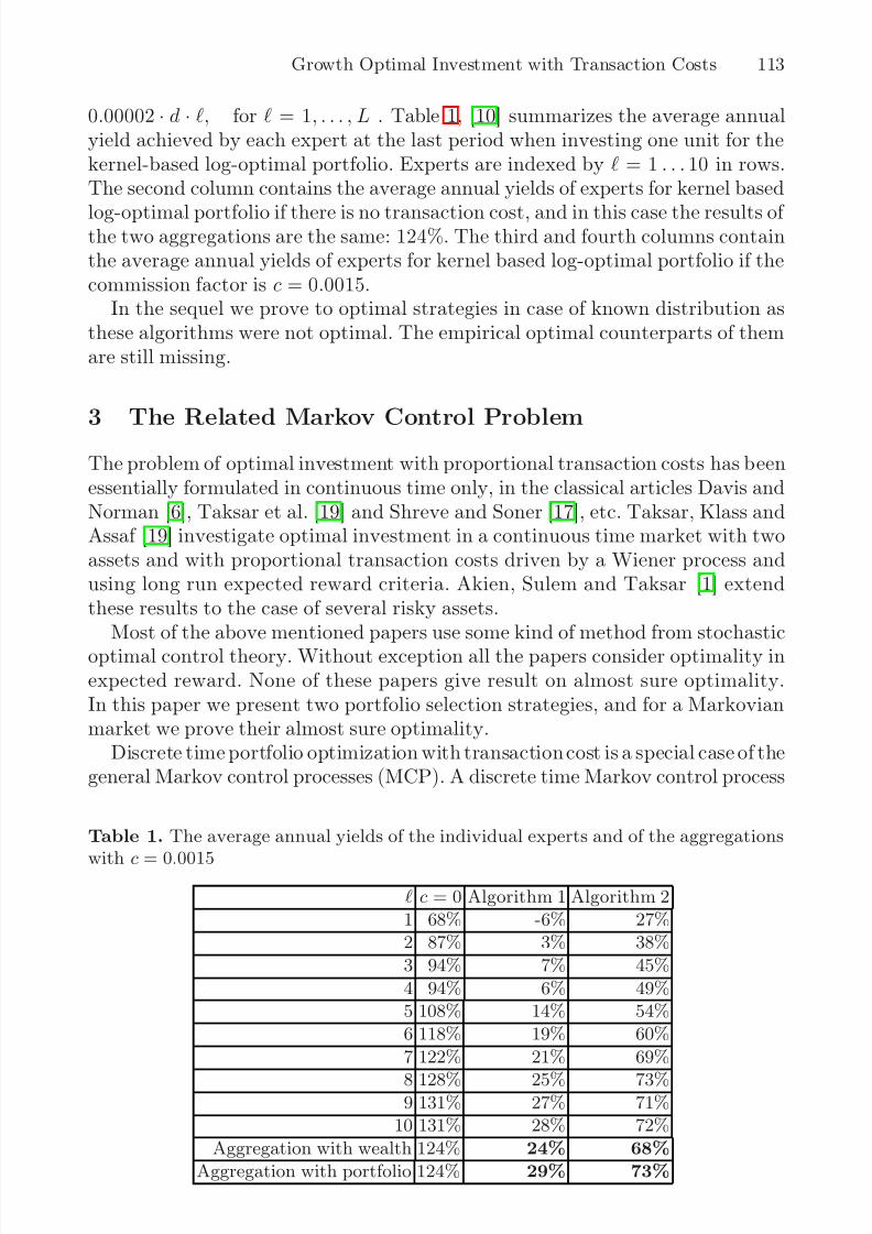
length 44 years - 11178 trading days ending in 2006 - achievable at www.szit.bme.hu/oti/portfolio. The proposed empirical portfolio selection algorithms use an in-finite set of experts. In the experiment we selected L = 10. Choose {q} = 1/Lover the experts in use, and the radius r2 = 0.0001 · d · , r2 = 0.0002 · d +
8/9/2019 Growth Optimal Portfolio Selection Strategies With Transaction Costs
http://slidepdf.com/reader/full/growth-optimal-portfolio-selection-strategies-with-transaction-costs 6/15
Growth Optimal Investment with Transaction Costs 113
0.00002 · d · , for = 1, . . . , L . Table 1, [10] summarizes the average annualyield achieved by each expert at the last period when investing one unit for thekernel-based log-optimal portfolio. Experts are indexed by = 1 . . . 10 in rows.The second column contains the average annual yields of experts for kernel based
log-optimal portfolio if there is no transaction cost, and in this case the results of the two aggregations are the same: 124%. The third and fourth columns containthe average annual yields of experts for kernel based log-optimal portfolio if thecommission factor is c = 0.0015.
In the sequel we prove to optimal strategies in case of known distribution asthese algorithms were not optimal. The empirical optimal counterparts of themare still missing.
3 The Related Markov Control Problem
The problem of optimal investment with proportional transaction costs has beenessentially formulated in continuous time only, in the classical articles Davis andNorman [6], Taksar et al. [19] and Shreve and Soner [17], etc. Taksar, Klass andAssaf [19] investigate optimal investment in a continuous time market with twoassets and with proportional transaction costs driven by a Wiener process andusing long run expected reward criteria. Akien, Sulem and Taksar [1] extendthese results to the case of several risky assets.
Most of the above mentioned papers use some kind of method from stochasticoptimal control theory. Without exception all the papers consider optimality inexpected reward. None of these papers give result on almost sure optimality.In this paper we present two portfolio selection strategies, and for a Markovianmarket we prove their almost sure optimality.
Discrete time portfolio optimization with transaction cost is a special case of thegeneral Markov control processes (MCP). A discrete time Markov control process
Table 1. The average annual yields of the individual experts and of the aggregations
withc = 0.0015
c = 0 Algorithm 1 Algorithm 2
1 68% -6% 27%2 87% 3% 38%
3 94% 7% 45%
4 94% 6% 49%5 108% 14% 54%
6 118% 19% 60%
7 122% 21% 69%
8 128% 25% 73%9 131% 27% 71%
10 131% 28% 72%
Aggregation with wealth 124% 24% 68%
Aggregation with portfolio 124% 29% 73%

8/9/2019 Growth Optimal Portfolio Selection Strategies With Transaction Costs
http://slidepdf.com/reader/full/growth-optimal-portfolio-selection-strategies-with-transaction-costs 7/15
114 L. Györfi and I. Vajda
is defined by a five tuple (S,A,U (s), Q , r) (cf. [11]). S is a Borel space, called thestate space, the action space A is Borel, too, the space of admissible actions U (s)is a Borel subset of A. Let the set K be {(s, a) : s ∈ S, a ∈ U (s)}. The transitionlaw is a stochastic kernel Q(.|s, a) on S given K , and r(s, a) is the reward function.
The evolution of the process is the following. Let S t denote the the state attime t, action At is chosen at that time. Let S t = s and At = a , then the rewardis r(s, a), and the process moves to S t+1 according to the kernel Q(.|s, a). Acontrol policy is a sequence π = {πn} of deterministic functions, which can alsobe stochastic kernels on A given the past states and actions.
Two reward criteria are considered. The expected long run average reward forπ is defined by J (π) = lim inf n→∞
1n
n−1t=0 E
πr(S t, At). The sample-path average
reward is defined as J (π) := lim inf n→∞1n
n−1t=0 r(S t, At). In the theory of MCP
most of the results correspond to expected long run average reward, while just
a few present result for the sample-path criterion. Such sample-path results canbe found in [3] for bounded rewards and in [20], [14] for unbounded rewards. ForMarkov control processes, the main aim is to approach the maximum asymptoticreward: J ∗ = supπ J (π), which leads to a dynamic programming problem.
For portfolio optimization with transaction cost, we formulate the correspond-ing Markov control problem. Assume that there exist 0 < a1 < 1 < a2 < ∞ suchthat
Xi ∈ [a1, a2]d
.
1. Let us define the state space as: S :=
(b
,x
)|b
∈ Δd,x
∈ [a1, a2]
d.
2. The action space is A := Δd.3. For the set of admissible actions we get U (b,x) := Δd.4. The stochastic kernel is Q(d(b,x)|(b,x),b) := P (dx|x) := P{dX2 =dx|X1 =x} the transition probability distribution of the Markov market process,describing the asset returns. Note, that this corresponds to the assumption, thatthe market behaviour is not affected by the investor.5. The reward function is: r((b,x),b) = v(b,b,x).6. The sample-path average reward criterion is the following:
lim inf n→∞1nn
t=1 r((bt−1,xt−1),bt) = lim inf n→∞1nn
t=1 v(bt−1,bt,xt−1)= lim inf n→∞ J n.
Remark 3. It should be noted that the methods of MCP literature, more pre-cisely the theorems in [3], [20], [14] can’t be applied in our case. However, wedo use the formalism, the results on the existence of the solution of discountedBellman equations, and the basic idea of vanishing discount approach.
4 Optimal Portfolio Selection Algorithms
We introduce two optimal portfolio selection strategies. Let 0 < δ < 1 denote adiscount factor. We apply a kind of vanishing discount approach, formulated bythe discounted Bellman equation:
F δ(b,x) = maxb
{v(b,b,x) + (1 − δ)E{F δ(b,X2) | X1 = x}} . (8)
8/9/2019 Growth Optimal Portfolio Selection Strategies With Transaction Costs
http://slidepdf.com/reader/full/growth-optimal-portfolio-selection-strategies-with-transaction-costs 8/15
Growth Optimal Investment with Transaction Costs 115
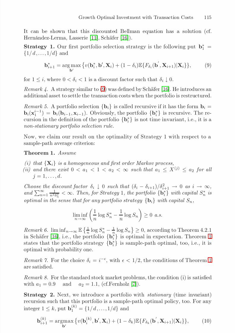
It can be shown that this discounted Bellman equation has a solution (cf.Hernández-Lerma, Lasserie [11], Schäfer [16]).
Strategy 1. Our first portfolio selection strategy is the following put b∗1 =
{1/ d , . . . , 1/d} and
b∗i+1 = arg max
b
v(b∗i ,b,Xi) + (1 − δi)E{F δi(b
,Xi+1)|Xi}}, (9)
for 1 ≤ i, where 0 < δi < 1 is a discount factor such that δi ↓ 0.
Remark 4. A strategy similar to (9) was defined by Schäfer [16]. He introduces anadditional asset to settle the transaction costs when the portfolio is restructured.
Remark 5. A portfolio selection {bi} is called recursive if it has the form bi =bi(x
i−1
1
) = bi(bi−1,xi−1). Obviously, the portfolio {b∗i
} is recursive. The re-cursion in the definition of the portfolio {b∗i } is not time invariant, i.e., it is anon-stationary portfolio selection rule .
Now, we claim our result on the optimality of Strategy 1 with respect to asample-path average criterion:
Theorem 1. Assume
(i) that {Xi} is a homogeneous and first order Markov process,(ii) and there exist 0 < a1 < 1 < a2 < ∞ such that a1 ≤ X (j) ≤ a2 for all
j = 1, . . . , d.
Choose the discount factor δi ↓ 0 such that (δi − δi+1)/δ2i+1 → 0 as i → ∞,and
∞n=1
1n2δ2n
< ∞. Then, for Strategy 1, the portfolio {b∗i } with capital S ∗n is
optimal in the sense that for any portfolio strategy {bi} with capital S n,
lim inf n→∞
1
nlog S ∗n −
1
nlog S n
≥ 0 a.s.
Remark 6. lim inf n→∞
E 1
n
log S ∗n
− 1
n
log S n ≥ 0, according to Theorem 4.2.1in Schäfer [16], i.e., the portfolio {b∗i } is optimal in expectation. Theorem 1states that the portfolio strategy {b∗i } is sample-path optimal, too, i.e., it isoptimal with probability one.
Remark 7. For the choice δi = i−, with < 1/2, the conditions of Theorem 1are satisfied.
Remark 8. For the standard stock market problems, the condition (i) is satisfiedwith a1 = 0.9 and a2 = 1.1, (cf.Fernholz [7]).
Strategy 2. Next, we introduce a portfolio with stationary (time invariant)recursion such that this portfolio is a sample-path optimal policy, too. For any
integer 1 ≤ k, put b(k)1 = {1/ d , . . . , 1/d} and
b(k)i+1 = argmax
b
v(b
(k)i ,b,Xi) + (1 − δk)E{F δk(b
,Xi+1)|Xi}}, (10)
8/9/2019 Growth Optimal Portfolio Selection Strategies With Transaction Costs
http://slidepdf.com/reader/full/growth-optimal-portfolio-selection-strategies-with-transaction-costs 9/15
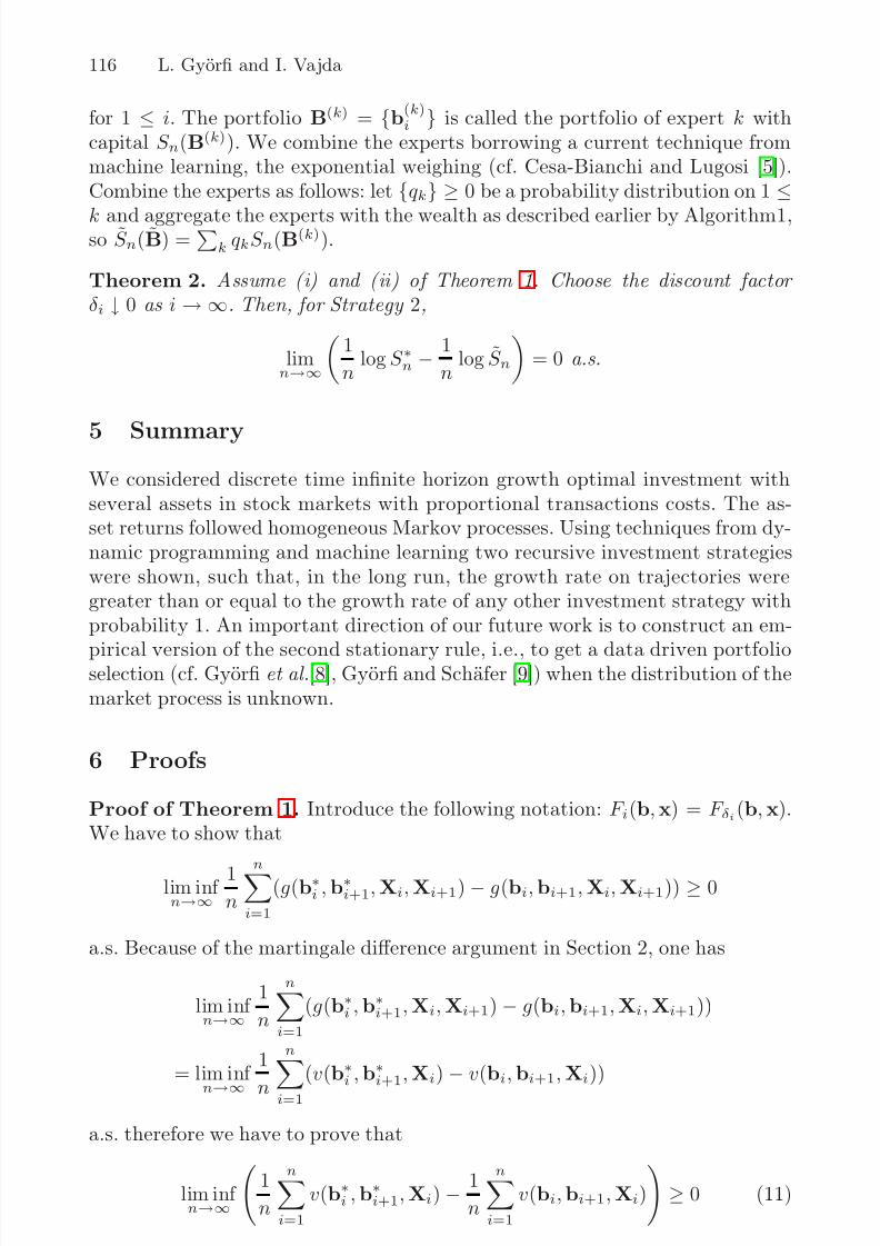
116 L. Györfi and I. Vajda
for 1 ≤ i. The portfolio B(k) = {b
(k)i } is called the portfolio of expert k with
capital S n(B(k)). We combine the experts borrowing a current technique frommachine learning, the exponential weighing (cf. Cesa-Bianchi and Lugosi [5]).Combine the experts as follows: let {qk} ≥ 0 be a probability distribution on 1 ≤
k and aggregate the experts with the wealth as described earlier by Algorithm1,so S̃ n(B̃) =
k qkS n(B(k)).
Theorem 2. Assume (i) and (ii) of Theorem 1. Choose the discount factor δi ↓ 0 as i → ∞. Then, for Strategy 2,
limn→∞
1
nlog S ∗n −
1
nlog S̃ n
= 0 a.s.
5 Summary
We considered discrete time infinite horizon growth optimal investment withseveral assets in stock markets with proportional transactions costs. The as-set returns followed homogeneous Markov processes. Using techniques from dy-namic programming and machine learning two recursive investment strategieswere shown, such that, in the long run, the growth rate on trajectories weregreater than or equal to the growth rate of any other investment strategy withprobability 1. An important direction of our future work is to construct an em-
pirical version of the second stationary rule, i.e., to get a data driven portfolioselection (cf. Györfi et al.[8], Györfi and Schäfer [9]) when the distribution of themarket process is unknown.
6 Proofs
Proof of Theorem 1. Introduce the following notation: F i(b,x) = F δi(b,x).We have to show that
lim inf n→∞
1n
ni=1
(g(b∗i ,b∗i+1,Xi,Xi+1) − g(bi,bi+1,Xi,Xi+1)) ≥ 0
a.s. Because of the martingale difference argument in Section 2, one has
lim inf n→∞
1
n
ni=1
(g(b∗i ,b∗i+1,Xi,Xi+1) − g(bi,bi+1,Xi,Xi+1))
= lim inf n→∞
1
n
n
i=1
(v(b∗i ,b∗i+1,Xi) − v(bi,bi+1,Xi))
a.s. therefore we have to prove that
lim inf n→∞
1
n
ni=1
v(b∗i ,b∗i+1,Xi) −1
n
ni=1
v(bi,bi+1,Xi)
≥ 0 (11)
8/9/2019 Growth Optimal Portfolio Selection Strategies With Transaction Costs
http://slidepdf.com/reader/full/growth-optimal-portfolio-selection-strategies-with-transaction-costs 10/15
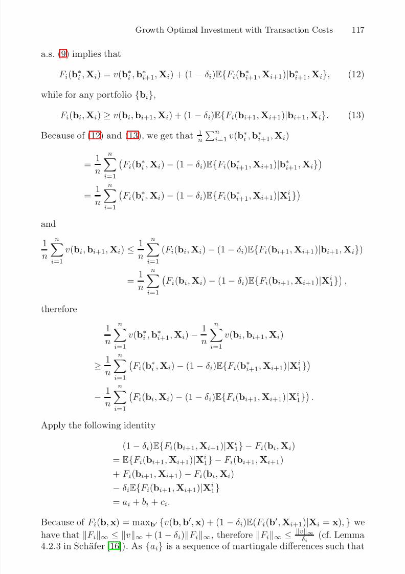
Growth Optimal Investment with Transaction Costs 117
a.s. (9) implies that
F i(b∗i ,Xi) = v(b∗i ,b∗i+1,Xi) + (1 − δi)E{F i(b
∗i+1,Xi+1)|b∗i+1,Xi}, (12)
while for any portfolio {bi},
F i(bi,Xi) ≥ v(bi,bi+1,Xi) + (1 − δi)E{F i(bi+1,Xi+1)|bi+1,Xi}. (13)
Because of (12) and (13), we get that 1n
n
i=1 v(b∗i ,b∗i+1,Xi)
=1
n
ni=1
F i(b
∗i ,Xi) − (1 − δi)E{F i(b∗i+1,Xi+1)|b∗i+1,Xi}
=1
n
n
i=1
F i(b∗
i,Xi) − (1 − δi)E{F i(b∗
i+1,Xi
+1)|Xi
1}
and
1
n
ni=1
v(bi,bi+1,Xi) ≤1
n
ni=1
(F i(bi,Xi) − (1 − δi)E{F i(bi+1,Xi+1)|bi+1,Xi})
=1
n
n
i=1 F i(bi,Xi) − (1 − δi)E{F i(bi+1,Xi+1)|Xi
1}
,
therefore
1
n
ni=1
v(b∗i ,b∗i+1,Xi) −1
n
ni=1
v(bi,bi+1,Xi)
≥1
n
ni=1
F i(b
∗i ,Xi) − (1 − δi)E{F i(b
∗i+1,Xi+1)|Xi
1}
−1
n
n
i=1
F i(b
i,X
i) − (1 − δ
i)E{F
i(b
i+1,X
i+1)|Xi
1} .
Apply the following identity
(1 − δi)E{F i(bi+1,Xi+1)|Xi1} − F i(bi,Xi)
= E{F i(bi+1,Xi+1)|Xi1} − F i(bi+1,Xi+1)
+ F i(bi+1,Xi+1) − F i(bi,Xi)
− δiE{F i(bi+1,Xi+1)|Xi1}
= ai + bi + ci.
Because of F i(b,x) = maxb {v(b,b,x) + (1 − δi)E(F i(b,Xi+1)|Xi = x), } we
have that F i∞ ≤ v∞ + (1 − δi)F i∞, therefore F i∞ ≤ v∞δi
(cf. Lemma4.2.3 in Schäfer [16]). As {ai} is a sequence of martingale differences such that
8/9/2019 Growth Optimal Portfolio Selection Strategies With Transaction Costs
http://slidepdf.com/reader/full/growth-optimal-portfolio-selection-strategies-with-transaction-costs 11/15
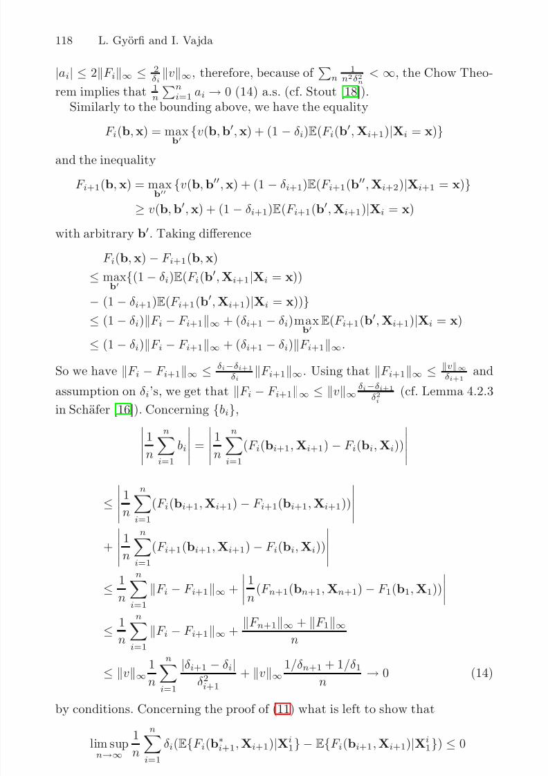
118 L. Györfi and I. Vajda
|ai| ≤ 2F i∞ ≤ 2δi
v∞, therefore, because of
n1
n2δ2n< ∞, the Chow Theo-
rem implies that 1n
ni=1 ai → 0 (14) a.s. (cf. Stout [18]).
Similarly to the bounding above, we have the equality
F i(b
,x
) = maxb {v(b
,b
,x
) + (1 − δi)E
(F i(b
,X
i+1)|X
i =x
)}
and the inequality
F i+1(b,x) = maxb
{v(b,b,x) + (1 − δi+1)E(F i+1(b,Xi+2)|Xi+1 = x)}
≥ v(b,b,x) + (1 − δi+1)E(F i+1(b,Xi+1)|Xi = x)
with arbitrary b. Taking difference
F i(b,x) − F i+1(b,x)
≤ maxb
{(1 − δi)E(F i(b,Xi+1|Xi = x))
− (1 − δi+1)E(F i+1(b,Xi+1)|Xi = x))}
≤ (1 − δi)F i − F i+1∞ + (δi+1 − δi)maxb
E(F i+1(b,Xi+1)|Xi = x)
≤ (1 − δi)F i − F i+1∞ + (δi+1 − δi)F i+1∞.
So we have F i − F i+1∞ ≤ δi−δi+1δi
F i+1∞. Using that F i+1∞ ≤ v∞δi+1
and
assumption on δi’s, we get that F i − F i+1∞ ≤ v∞δi−δi+1
δ2i(cf. Lemma 4.2.3
in Schäfer [16]). Concerning {bi}, 1
n
ni=1
bi
=
1
n
ni=1
(F i(bi+1,Xi+1) − F i(bi,Xi))
≤
1
n
ni=1
(F i(bi+1,Xi+1) − F i+1(bi+1,Xi+1))
+ 1n
ni=1
(F i+1(bi+1,Xi+1) − F i(bi,Xi))
≤1
n
ni=1
F i − F i+1∞ +
1
n(F n+1(bn+1,Xn+1) − F 1(b1,X1))
≤
1
n
ni=1
F i − F i+1∞ +F n+1∞ + F 1∞
n
≤ v∞
1
n
n
i=1
|δi+1 − δi|
δ2i+1 + v∞
1/δn+1 + 1/δ1
n → 0 (14)
by conditions. Concerning the proof of (11) what is left to show that
lim supn→∞
1
n
ni=1
δi(E{F i(b∗i+1,Xi+1)|Xi
1} − E{F i(bi+1,Xi+1)|Xi1}) ≤ 0
8/9/2019 Growth Optimal Portfolio Selection Strategies With Transaction Costs
http://slidepdf.com/reader/full/growth-optimal-portfolio-selection-strategies-with-transaction-costs 12/15
Growth Optimal Investment with Transaction Costs 119
a.s. The definition of F i implies that
F i(b∗i+1,Xi+1) − F i(bi+1,Xi+1)
= maxb v(b∗i+1,b,Xi+1) + (1 − δi)E{F i(b
,Xi+2)|Xi+1}− max
b
v(bi+1,b,Xi+1) + (1 − δi)E{F i(b
,Xi+2)|Xi+1}
≤ maxb
v(b∗i+1,b,Xi+1) + (1 − δi)E{F i(b
,Xi+2)|Xi+1}
−v(bi+1,b,Xi+1) − (1 − δi)E{F i(b,Xi+2)|Xi+1}
≤ max
b
v(b∗i+1,b,Xi+1) − v(bi+1,b,Xi+1)
≤ 2v∞,
therefore
1
n
ni=1
δiE{F i(b∗i+1,Xi+1) − F i(bi+1,Xi+1)|Xi
1} ≤2v∞
n
ni=1
δi → 0. (15)
(6), (14) and (15) imply (11).
Proof of Theorem 2
Theorem 1 implies that lim inf n→∞ 1n
log S ∗n − 1n
log S̃ n ≥ 0 a.s.. We have to
show that
lim inf n→∞
1
nlog S̃ n −
1
nlog S ∗n
≥ 0 (16)
a.s. By definition, 1n
log S̃ n = 1n
log∞
k=1 qkS n(B(k)) ≥ 1n
log supk qkS n(B(k)) =
supk
log qkn
+ 1n
log S n(B(k))
, therefore (16) follows from the following:
lim inf n→∞
supk
log qkn
+ 1n
ni=1 g(b
(k)i ,b
(k)i+1,Xi,Xi+1)
− 1
n n
i=1 g(b∗i ,b∗i+1,Xi,Xi+1) ≥ 0 a.s. which is equivalent to
lim inf n→∞
supk
log qkn
+1
n
ni=1
(v(b(k)i ,b
(k)i+1,Xi) − v(b∗i ,b∗i+1,Xi))
≥ 0 (17)
a.s. (10) implies that
F k(b(k)i ,Xi) = v(b
(k)i ,b
(k)i+1,Xi) + (1 − δk)E{F k(b
(k)i+1,Xi+1)|b
(k)i+1,Xi}, (18)
while for any portfolio {bi},
F k(bi,Xi) ≥ v(bi,bi+1,Xi) + (1 − δk)E{F k(bi+1,Xi+1)|bi+1,Xi},
thus for the portfolio {b∗i }
F k(b∗i ,Xi) ≥ v(b∗i ,b∗i+1,Xi) + (1 − δk)E{F k(b∗i+1,Xi+1)|b∗i+1,Xi}. (19)
8/9/2019 Growth Optimal Portfolio Selection Strategies With Transaction Costs
http://slidepdf.com/reader/full/growth-optimal-portfolio-selection-strategies-with-transaction-costs 13/15
120 L. Györfi and I. Vajda
Because of (18) and (19), we get that 1n
ni=1 v(b∗i ,b∗i+1,Xi) ≤
≤1
n
n
i=1
F k(b∗i ,Xi) − (1 − δk)E{F k(b∗i+1,Xi+1)|b∗i+1,Xi}=
1
n
ni=1
F k(b∗i ,Xi) − (1 − δk)E{F k(b∗i+1,Xi+1)|Xi
1}
and 1n
n
i=1 v(b(k)i ,b
(k)i+1,Xi) =
=1
n
ni=1
F k(b
(k)i ,Xi) − (1 − δk)E{F k(b
(k)i+1,Xi+1)|b
(k)i+1,Xi}
=1
n
ni=1
F k(b
(k)i ,Xi) − (1 − δk)E{F k(b
(k)i+1,Xi+1)|X
i1}
,
therefore
1
n
ni=1
v(b(k)i ,b
(k)i+1,Xi) −
1
n
ni=1
v(b∗i ,b∗i+1,Xi)
≥1
n
ni=1
F k(b
(k)i ,Xi) − (1 − δk)E{F k(b
(k)i+1,Xi+1)|Xi
1}
− 1n
ni=1
F k(b∗i ,Xi) − (1 − δk)E{F k(b∗i+1,Xi+1)|Xi
1}
.
Apply the following identity
(1 − δk)E{F k(bi+1,Xi+1)|Xi1} − F k(bi,Xi)
= E{F k(bi+1,Xi+1)|Xi1} − F k(bi+1,Xi+1) + F k(bi+1,Xi+1) − F k(bi,Xi)
− δkE{F k(bi+1,Xi+1)|Xi1}
= ai + bi + ci.Similarly to the proof of Theorem 1, the averages of ai’s and bi’s tend to zeroa.s., so concerning (17) we have that, with probability one,
lim inf n→∞
supk
log qkn
+1
n
ni=1
(v(b(k)i ,b
(k)i+1,Xi) − v(b∗i ,b∗i+1,Xi))
≥ supk
lim inf n→∞
log qkn
+1
n
n
i=1
(v(b(k)i ,b
(k)i+1,Xi) − v(b∗i ,b∗i+1,Xi))
= supk
lim inf n→∞
1
n
ni=1
(v(b(k)i ,b
(k)i+1,Xi) − v(b∗i ,b∗i+1,Xi))
= supk
lim inf n→∞
δkn
ni=1
(E{F k(b(k)i+1,Xi+1)|Xi
1} − E{F k(b∗i+1,Xi+1)|Xi1}).
8/9/2019 Growth Optimal Portfolio Selection Strategies With Transaction Costs
http://slidepdf.com/reader/full/growth-optimal-portfolio-selection-strategies-with-transaction-costs 14/15
Growth Optimal Investment with Transaction Costs 121
The problem left is to show that the last term is non negative a.s. Using thedefinition of F k
F k(b(k)i+1,Xi+1) − F k(b∗i+1,Xi+1)
= maxb
v(b(k)i+1,b,Xi+1) + (1 − δk)E{F k(b
,Xi+2)|Xi+1}
− maxb
v(b∗i+1,b,Xi+1) + (1 − δk)E{F k(b,Xi+2)|Xi+1}
= max
bminb
v(b
(k)i+1,b,Xi+1) + (1 − δk)E{F k(b
,Xi+2)|Xi+1}
−
v(b∗i+1,b,Xi+1) + (1 − δk)E{F k(b,Xi+2)|Xi+1}
≥ minb
v(b
(k)i+1,b,Xi+1) + (1 − δk)E{F k(b,Xi+2)|Xi+1}
−v(b∗i
+1
,b,Xi+1) + (1 − δk)E{F k(b,Xi+2)|Xi+1}= min
b
v(b
(k)i+1,b,Xi+1) − v(b∗i+1,b,Xi+1)
≥ −2v∞,
therefore
supk
lim inf n→∞
δkn
ni=1
E{F k(b(k)i+1,Xi+1) − F k(b∗i+1,Xi+1)|Xi
1} ≥ supk
δk(−2v∞)
= 0
a.s., and (17) is proved.
References
[1] Akien, M., Sulem, A., Taksar, M.I.: Dynamic Optimization of Long-term GrowthRate for a Portfolio with Transaction Costs and Logaritmic Utility. MathematicalFinance 11, 153–188 (2001)
[2] Algoet, P., Cover, T.: Asymptotic Optimality Asymptotic Equipartition Proper-
ties of Log-optimum Investments. Annals of Probability 16, 876–898 (1988)[3] Arapostathis, A., Borkar, V.S., Fernandez-Gaucherand, E., Ghosh, M.K., Marcus,
S.I.: Discrete-time Controlled Markov Processes with Average Cost Criterion: aSurvey. SIAM J. Control Optimization 31, 282–344 (1993)
[4] Bobryk, R.V., Stettner, L.: Discrete Time Portfolio Selection with ProportionalTransaction Costs. Probability and Mathematical Statistics 19, 235–248 (1999)
[5] Cesa-Bianchi, N., Lugosi, G.: Prediction, Learning, and Games. Cambridge Uni-versity Press, Cambridge (2006)
[6] Davis, M.H.A., Norman, A.R.: Portfolio Selection with Transaction Costs. Math-ematics of Operations Research 15, 676–713 (1990)
[7] Fernholz, E.R.: Stochastic Portfolio Theory. Springer, New York (2000)[8] Györfi, L., Lugosi, G., Udina, F.: Nonparametric Kernel-based Sequential Invest-
ment Strategies. Mathematical Finance 16, 337–357 (2006)[9] Györfi, L., Schäfer, D.: Nonparametric Prediction. In: Suykens, J.A.K., Horváth,
G., Basu, S., Micchelli, C., Vandevalle, J. (eds.) Advances in Learning Theory:Methods, Models and Applications, pp. 339–354. IOS Press, Amsterdam (2003)

8/9/2019 Growth Optimal Portfolio Selection Strategies With Transaction Costs
http://slidepdf.com/reader/full/growth-optimal-portfolio-selection-strategies-with-transaction-costs 15/15
122 L. Györfi and I. Vajda
[10] Györfi, L., Ottucsák, G.: Empirical log-optimal portfolio selections: a survey, man-uscript (2007),http://www.szit.bme.hu/oti/portfolio/articles/tgyorfi.pdf
[11] Hernández-Lerma, L., Lasserre, J.B.: Discrete-Time Markov Control Processes:Basic Optimality Criteria. Springer, New York (1996)
[12] Iyengar, G.: Discrete Time Growth Optimal Investment with Costs. Working Pa-per (2002), http://www.columbia.edu/gi10/Papers/stochastic.pdf
[13] Iyengar, G., Cover, T.: Growth Optimal Investment in Horse Race Markets withCosts. IEEE Transactions on Information Theory 46, 2675–2683 (2000)
[14] Lasserre, J.B.: Sample-path Average Optimality for Markov Control Processes.IEEE Transactions on Automatic Control 44, 1966–1971 (1999)
[15] Palczewski, J., Stettner, L.: Optimisation of Portfolio Growth Rate on the Marketwith Fixed Plus Proportional Transaction Cost. CIS to Appear a Special IssueDedicated to Prof. T. Duncan (2006)
[16] Schäfer, D.: Nonparametric Estimation for Finantial Investment under Log-Utility. PhD Dissertation, Mathematical Institute, University Stuttgart. ShakerVerlag, Aachen (2002)
[17] Shreve, S.E., Soner, H.M.: Optimal Investment and Consumption with Transac-tion Costs. Annals of Applied Probability 4, 609–692 (1994)
[18] Stout, W.F.: Almost Sure Convergence. Academic Press, New York (1974)[19] Taksar, M., Klass, M., Assaf, D.: A Diffusion Model for Optimal Portfolio Selection
in the Presence of Brokerage Fees. Mathematics of Operations Research 13, 277–294 (1988)
[20] Vega-Amaya, O.: Sample-path Average Optimality of Markov Control Processes
with Strictly Unbounded Costs. Applicationes Mathematicae 26, 363–381 (1999)