Harmonic Analysis

Lectures by Pascal AuscherTypeset by Lashi Bandara

June 8, 2010

Contents

1 Measure Theory 2

2 Coverings and cubes 4

2.1 Vitali and Besicovitch . . . . . . . . . . . . . . . . . . . . . . . . . . . . . . 4

2.2 Dyadic Cubes . . . . . . . . . . . . . . . . . . . . . . . . . . . . . . . . . . . 8

2.3 Whitney coverings . . . . . . . . . . . . . . . . . . . . . . . . . . . . . . . . 9

3 Maximal functions 14

3.1 Centred Maximal function on Rn . . . . . . . . . . . . . . . . . . . . . . . . 14

3.2 Maximal functions for doubling measures . . . . . . . . . . . . . . . . . . . 17

3.3 The Dyadic Maximal function . . . . . . . . . . . . . . . . . . . . . . . . . . 19

3.4 Maximal Function on Lp spaces . . . . . . . . . . . . . . . . . . . . . . . . . 21

4 Interpolation 26

4.1 Real interpolation . . . . . . . . . . . . . . . . . . . . . . . . . . . . . . . . 26

4.2 Complex interpolation . . . . . . . . . . . . . . . . . . . . . . . . . . . . . . 29

5 Bounded Mean Oscillation 35

5.1 Construction and properties of BMO . . . . . . . . . . . . . . . . . . . . . . 35

5.2 John-Nirenberg inequality . . . . . . . . . . . . . . . . . . . . . . . . . . . . 39

5.3 Good λ inequalities and sharp maximal functions . . . . . . . . . . . . . . . 42

i

6 Hardy Spaces 48

6.1 Atoms and H1 . . . . . . . . . . . . . . . . . . . . . . . . . . . . . . . . . . . 48

6.2 H1 − BMO Duality . . . . . . . . . . . . . . . . . . . . . . . . . . . . . . . . 52

7 Calderon-Zygmund Operators 55

7.1 Calderon-Zygmund Kernels and Operators . . . . . . . . . . . . . . . . . . . 55

7.2 The Hilbert Transform, Riesz Transforms, and The Cauchy Operator . . . . 57

7.2.1 The Hilbert Transform . . . . . . . . . . . . . . . . . . . . . . . . . . 57

7.2.2 Riesz Transforms . . . . . . . . . . . . . . . . . . . . . . . . . . . . . 59

7.2.3 Cauchy Operator . . . . . . . . . . . . . . . . . . . . . . . . . . . . . 61

7.3 Lp boundedness of CZOα operators . . . . . . . . . . . . . . . . . . . . . . . 62

7.4 CZO and H1 . . . . . . . . . . . . . . . . . . . . . . . . . . . . . . . . . . . 67

7.5 Mikhlin multiplier Theorem . . . . . . . . . . . . . . . . . . . . . . . . . . . 69

7.6 Littlewood-Paley Theory . . . . . . . . . . . . . . . . . . . . . . . . . . . . . 71

8 Carleson measures and BMO 76

8.1 Geometry of Tents and Cones . . . . . . . . . . . . . . . . . . . . . . . . . . 77

8.2 BMO and Carleson measures . . . . . . . . . . . . . . . . . . . . . . . . . . 80

9 Littlewood Paley Estimates 91

10 T (1) Theorem for Singular Integrals 96

Notation 105

1

Chapter 1

Measure Theory

While we shall focus our attention primarily on Rn, we note some facts about measuresin an abstract setting and in the absence of proofs.

Let X be a set. The reader will recall that in the literature, a measure µ on X is usuallydefined on a σ-algebra M ⊂ P(X). This approach is limited in the direction we willtake. In the sequel, it will be convenient to forget about measurability and associate a sizeto arbitrary subsets but still in a meaningful way. We present the Caratheodory’s notionof measure and measurability. In the literature, what we call a measure is sometimesdistinguished as an outer measure.

Definition 1.0.1 (Measure/Outer measure). Let X be a set. Then, a map µ : P(X)→[0,+∞] is called a measure on X if it satisfies:

(i) µ(∅) = 0,

(ii) µ(A) ≤∑∞

i=1 µ(Ai) whenever A ⊂⋃∞i=1Ai.

Remark 1.0.2. Note that (ii) includes the statement: if A ⊂ B, then µ(A) ≤ µ(B).

Certainly, the classical measures are additive on disjoint subsets. This is something welose in the definition above. However, we can recover both the measure σ-algebra and anotion of measurable set.

Definition 1.0.3 (Measurable). Let µ be a measure on X (in the sense of Definition1.0.1). We say A ⊂ X is µ-measurable if for all Y ⊂ X,

µ(A) = µ(A \ Y ) + µ(A ∩ Y ).

Theorem 1.0.4. Let Ai∞i=1 be a countable set of µ-measurable sets. Then,

(i)⋂∞i=1Ai and

⋃∞i=1Ai are µ-measurable,

(ii) If the sets Ai∞i=1 are mutually disjoint, then

µ

( ∞⋃i=1

Ai

)=∞∑i=1

µ(Ai),

2

(iii) If Ak ⊂ Ak+1 for all k ≥ 1, then

limk→∞

µ(Ak) = µ

( ∞⋃i=1

Ai

),

(iv) If Ak ⊃ Ak+1 for all k ≥ 1, then

limk→∞

µ(Ak) = µ

( ∞⋂i=1

Ai

),

(v) The set M = A ⊂ X : A is µ−measurable is a σ-algebra.

A proof of (i) - (iv) can can be found in [GC91, p2]. Then, (v) is an easy consequence andwe leave it as an exercise.

The following result illustrates that we can indeed think about classical measures in thisframework. Recall that a measure space is a tripe (X,M , ν) where M ⊂ P(X) is a σ-algebra and ν : M → [0,+∞] is a measure in the classical sense. Measure spaces are alsogiven as the tuple (X,µ) by which we mean (X,M , ν) where M is the largest σ-algebracontaining measurable sets.

Theorem 1.0.5. Let (X,M , ν) be a measure space. Then, there exists an measure µ onX such that µ = ν on M .

See [G.81, §5.2, Theorem 3].

Of particular importance is the following construction of the Lebesgue measure in oursense.

Definition 1.0.6 (Lebesgue Measure). Let A ⊂ Rn. For a Euclidean ball B, denote thevolume of the ball by volB. Define the Lebesgue measure L :

L (A) = inf

∞∑i=1

volBi : A ⊂∞⋃i=1

Bi and each Bi is an open ball

.

This definition is justified by the following proposition.

Proposition 1.0.7. Let (Rn,M ′,L ′) be the classical Lebesgue measure defined on thelargest σ-algebra M ′ and let M = A ⊂ X : A is L −measurable. Then,

M ′ = M and L (A) = L ′(A)

for all A ∈M ′.

For a more detailed treatment of abstract measure theory, see [GC91, §1] and [G.81, Ch.5].

3

Chapter 2

Coverings and cubes

We will consider the setting of Rn with the usual Euclidean norm |· | inducing the standardEuclidean metric dE(x, y) = |x− y|. We note, however, that some of the material that wediscuss here can be easily generalised to a more abstract setting.

To introduce some nomenclature, we denote the ball centred at x with radius r > 0 byB(x, r). We are intentionally ambiguous as to whether the ball is open or closed. We willspecify when this becomes important.

For a ball B, let radB denote it’s radius. For λ > 0, we denote the ball with the samecentre but radius λ radB by λB.

This chapter is motivated by the following two questions.

(1) Suppose that Ω =⋃B∈B B where B is a family of balls. We wish to extract a

subfamily B′ of balls that do not overlap “too much” and still cover Ω.

(2) Given a set Ω ⊂ Rn, how can we select a cover of Ω with a given geometric structure.

2.1 Vitali and Besicovitch

Lemma 2.1.1 (Vitali Covering Lemma). Let Bαα∈I be a family of balls in Rn andsuppose that

supα∈I

radBα <∞.

Then there exists a subset I0 ⊂ I such that

(i) Bαα∈I0 are mutually disjoint.

(ii)⋃α∈I Bα ⊂

⋃α∈I0 5Bα.

Remark 2.1.2. (i) The balls Bαα∈I can be open or closed.

4

(ii) This statement only relies on the metric structure of Rn with the euclidean metricgiven by |· |. It can be replaced by a metric space (E, d). As an example, we can set(E, d) = (Rn, d∞), where d∞ is the infinity distance given be by the infinity norm.This is equivalent to replacing balls by cubes.

(iii) The condition supα∈I radBα <∞ is necessary. A counterexample is Bi = B(0, i) : i ∈ N.

(iv) The optimal constant is not 5, it is 3, but somewhat complicates the proof.

Proof. Let M = supα∈I radBα. For j ∈ N, define

I(j) =α ∈ I : 2−j−1M < radBα ≤ 2−jM

.

We inductively extract maximal subsets of each I(j). So, for j = 0, let J(0) be a maximalsubset of I(0) such that Bαα∈J(0) are mutually disjoint. The existence of such a collectionis guaranteed by Zorn’s Lemma. Now, for j = 1, we extract a maximal J(1) ⊂ I(1) suchthat Bαα∈J(1) mutually disjoint and also disjoint from Bαα∈J(0). Now, when j = k,we let J(k) ⊂ I(k) be maximal such that Bαα∈J(k) mutually disjoint and disjoint fromBαα∈∪k−1

m=0J(m). We then let

I0 =⋃k∈N

J(k).

By construction, Bαα∈I0 are mutually disjoint. This proves (i).

To prove (ii), fix a ball Bα ∈ I. We show that there exists a β ∈ I0 such that Bα ⊂ 5Bβ.We have a k ∈ N such that α ∈ I(k). That is,

2−k−1M < radBα ≤ 2−kM.

If i ∈ J(k), then we’re done. So suppose not. By construction, this must mean that Bαmust intersect a ball Bβ for β ∈ J(l) where 0 ≤ l ≤ k. But we know that

radBβ ≥ 2−l−1M ≥ 2−k−1M ≥ 1

2radBα

and by the triangle inequality

d(xα, xβ) ≤ radBα + radBβ.

Then, radBα + d(xα, xβ) ≤ 2 radBα + radBβ ≤ 5 radBβ and so it follows that

Bα = B(xα, radBα) ⊂ B(xβ, radBα + d(xα, xβ)) ⊂ B(xβ, 5 radBβ) = 5Bβ.

Before we introduce our next covering theorem, we require a rigorous notion of a family ofballs to not intersect “too much.” First, we note that χX denotes the indicator functionof B.

Definition 2.1.3 (Bounded Overlap). A collection of balls B is said to have boundedoverlap if there exists a C ∈ N such that∑

B∈B

χB ≤ C.

5

Theorem 2.1.4 (Besicovitch Covering Theorem). Let E ⊂ Rn. For each x ∈ E, let B(x)be a ball centred at x. Assume that E is bounded or that supx∈E radB(x) < ∞. Then,there exists a countable set E0 ⊂ E and a constant C(n) ∈ N such that

(i) E ⊂⋃x∈E0

B(x).

(ii)∑

x∈E0χB(x) ≤ C(n).

Remark 2.1.5. (i) Here, (ii) means that the set B(x)x∈E0forms a bounded covering

of E with constant C(n). This constant depends only on dimension. The boundedcovering property tells us that the balls are “almost disjoint.” In fact, we can organiseE0 = E1 ∪ . . . ∪ EN such that each set B(x)x∈Ek contain mutually disjoint balls.We will not prove this.

(ii) We can substitute cubes for balls.

(iii) For E unbounded, the condition supx∈E radB(x) <∞ is necessary.

(iv) This theorem is very special to Rn. A counterexample is the Heisenberg group.

(v) The balls must be centred at each point in E. Otherwise, consider E = [0, 1] andBi = [0, 1− 2i], i ≥ 1.

Before we proceed to prove the theorem, we require the following Lemma.

Lemma 2.1.6. For y ∈ Rn, let Cε(y) be the sector with vertex y with aperture angleε. Suppose that 0 < ε ≤ π/6. Then, for all R > 0, x, z ∈ Cε(y), if |x| , |z| ≤ R then|x− z| ≤ R.

Proof of Besicovitch Covering Theorem. Let M = supx∈E radB(x) and suppose that E isbounded and M = ∞. Then, fix an x0 ∈ E and there exists a ball B(x0, R) such thatB(x0, R) ⊃ E. Then, we’re done by setting E0 = x0.

So, we suppose now that E is bounded and M <∞. Define:

E(k) =x ∈ E : 2−k−1M < radB(x) ≤ 2−kM

.

We select points xj inductively from each E(k) to construct a set E′(k). So, fix an initialx0,0 ∈ E(0) and select x0,i ∈ E(0) by requiring that x0,i 6∈

⋃i−1l=0 B(x0,l). Then, for arbitrary

k > 0, assume that E′(0), . . . , E′(k−1) have already been constructed and construct E′(k)by selecting xk,i such that xk,i 6∈

⋃i−1l=0 B(xk,l) ∪k−1

m=1 ∪xm,i∈E′(m)B(xm,i). Each E′(k) mustbe finite since by the boundedness of E and the definition of E(k), this process must stopafter finitely many selections in E(k). Now, let E0 =

⋃k∈NE

′(k) with equipped with thenatural ordering. That is, E0 = x1, x2, . . . and if i < j then xj 6∈ B(xi). This is thesame as saying that xi was selected before xj .

We prove (i). Suppose x ∈ E but x 6∈⋃xi∈E0

B(xi). In particular this means thatx ∈ E′(k) for some k which is a contradiction.

6

Now, to show (ii), fix y ∈ Rn, let ε = π/6 and let Cε(y) denote the sector with vertex yand aperture ε. Define

Ay = xi ∈ E0 : y ∈ B(xi) and xi ∈ Cε(y) ,

and let i = minAy. Take xj ∈ Ay with j > i. Then,xi, xj ∈ Cε(y)

|xi − y| ≤ radB(xi)

|xj − y| ≤ radB(xj)

and so |xi − xj | ≤ max radB(xi), radB(xj) by application of Lemma 2.1.6. But by theordering on E0, xj was selected after xi and so xj 6∈ B(xi). Consequently radB(xj) ≤|xj − xi| which implies radB(xj) ≥ radB(xi).

Now, suppose that xi was selected at generation k, so 2−k−1M < radB(xi) ≤ 2−kM . Also,2−k−1M < radB(xj) ≤ 2−kM for otherwise, xj would be selected at a later generationl > k which implies that radB(xi) > radB(xj) which is a contradiction.

Also, note thatB(xj , 2

−k−2M) : j ∈ Ay

are mutually disjoint and are all contained inB(xi, 2

−k+1M). It follows that,∑j∈Ay

L (B(xj , 2−k−2M)) ≤ L (B(xi, 2

−k+1M) = (23)nL (B(0, 2−k−2M))

and

cardAy =∑j∈Ay

1 =∑j∈Ay

L (B(xj , 2−k−2M))

L (B(0, 2−k−2M))≤ 23n

and we are done.

We shall not give details for the case that E is unbounded, but it can be obtained fromthe previous case with some effort. We refer the reader to [GC91, p35].

Corollary 2.1.7 (Sard’s Theorem). Let f ∈ C1(Rn;Rn) and let

A =

x ∈ Rn : lim inf

r→0

L (f(B(x, r)))

L (B(x, r))= 0

.

Then L (f(A)) = 0. (Recall that by our definition of L , we can measure every subset ofRn).

Proof. Firstly, we note that for all x ∈ A and ε > 0, there exists an rx ∈ (0, 1] such that

L (f(B(x, rx))) ≤ εL (B(x, rx)).

LetA0 ⊂ A be the set of centres given by Besicovitch applied to the set of balls Bx = B(x, rx)for which the above measure condition holds. Then, f(A) ⊂

⋃xi∈A0

f(B(xi)) and by the

7

subadditivity of L ,

L (f(A)) ≤∑xi∈A0

L (f(Bxi))

≤ ε∑xi∈A0

L (Bxi)

≤ εˆA∪B(0,1)

∑χBxi (y) dL (y)

≤ εC(n)L (A ∪B(0, 1)).

Now, if A is bounded, then L (A ∪ B(0, 1)) < ∞ and we can obtain the conclusion byletting ε → 0. Otherwise, we replace A by A ∩ B(0, k) to obtain L (f(A ∩ B(0, k))) = 0and then by taking k →∞ we establish L (f(A))) = 0.

2.2 Dyadic Cubes

We begin with the construction of dyadic cubes on Rn.

Definition 2.2.1 (Dyadic Cubes). Let [0, 1)n be the reference cube and let j ∈ Z andk = (k1, . . . , kn) ∈ Zn. Then define the dyadic cube of generation j with lower left corner2−jk

Qj,k =x ∈ Rn : 2jx− k ∈ [0, 1)n

,

the set of generation j dyadic cubes

Qj = Qj,k : k ∈ Zn ,

and the set of all cubes

Q =⋃j∈Z

Qj = Qj,k : j ∈ Z and k ∈ Zn .

We define the length of a cube to be its side length `(Qj,k) = 2−j.

Remark 2.2.2. If we were to replace [0, 1)n with R =∏ni=1[ai, ai+δ) as a reference cube,

then the dyadic cubes with respect to R are constructed via the homothety ϕ : Rn → Rnwhere ϕ([0, 1)n) = R.

Theorem 2.2.3 (Properties of Dyadic Cubes). (i) For j ∈ Z, `(Qj,k) = 2−j, L (Qj,k) =2−jn, and Qj forms a partition of Rn for each j ∈ Z.

(ii) For all j ∈ Z and k ∈ Zn, there exists a unique k′ ∈ Zn such that Qj,k ⊂ Qj−1,k′.

We set Qj,k = Qj−1,k′ and it is called the parent of Qj,k.

(iii) For all j ∈ Z and k ∈ Zn, the setQj+1,k′ : Qj+1,k′ = Qj,k

(that is, the set of cubes

Qj+1,k′ for which Qj,k is the parent) are called the children of Qj,k.

(iv) For all x ∈ Rn, there exists a unique sequence of dyadic cubes (Qj,kj )j∈Z ⊂ Q suchthat Qj+1,kj+1

is a child of Qj,k, Qj,kj is the parent of Qj+1,kj+1and x ∈ Qj,kj for

all j ∈ Z.

8

(v) Let E ⊂ Q such that Ω =⋃Q∈E Q and satisfying L (Ω) < ∞. Then, there exists a

collection F ⊂ Q of mutually disjoint dyadic cubes such that Ω =⋃Q′∈F Q′.

Proof. We leave it to the reader to verify (i) - (iv). We prove (v).

Define:

F =Q′ ∈ Q : Q′ ⊂ Ω but Q′ 6⊂ Ω

.

We prove that F 6= ∅. Let Q ∈ E , and denote the kth parent by Qk. It follows that

L (Qk) = (2n)kL (Q). Now, let k0 = maxk : Qk ⊂ Ω

and consequently, Qk0 ∈ F .

Now, note that⋃Q∈E Q ⊂

⋃Q′∈F Q′ and by the construction of F ,

⋃Q′∈F Q′ ⊂ Ω. But

by hypothesis Ω =⋃Q∈E Q and so it follows that Ω =

⋃Q′∈F Q′.

To complete the proof, we prove that F is mutually disjoint. Let Q′,Q′′ ∈ F and assumethat Q′ 6= Q′′. This is exactly that Q′ 6⊂ Q′′ and Q′ 6⊃ Q′′ so by (iii), Q′ ∩Q′′ = ∅.

Remark 2.2.4. (i) Suppose Ω is an open set with L (Ω) <∞ and let E = Q ∈ Q : Q ⊂ Ω.Then, F ⊂ E and we call F the maximal dyadic cubes in E . Maximality here iswith respect to the property Q ⊂ Ω.

(ii) The assumption L (Ω) <∞ cannot be dropped. A counterexample is [0, 2k) ⊂ R fork ∈ N.

2.3 Whitney coverings

The Whitney covering theorems are an important tool in Harmonic analysis. We initiallygive a dyadic version of Whitney. But first, we recall some terminology from the theory ofmetric spaces. Recall that the diameter of a set E ⊂ X for a metric space (X, d) is givenby

diamE = supx,y∈E

d(x, y),

and the distance from E to another set F ⊂ X is given by

dist(E,F ) = infx∈E,y∈F

d(x, y).

Then the distance from E to a point y ∈ X is simply given by dist(x,E) = dist(E,F )where F = x.

Theorem 2.3.1 (Whitney Covering Theorem for Dyadic cubes). Let O $ Rn be open.Then, there exists a collection of Dyadic cubes E = Qii∈I such that

(i)1

30dist(Qi, cO) ≤ diamQi ≤

1

10dist(Qi, cO),

9

(ii)

O =⋃i∈IQi,

(iii) The dyadic cubes in E are mutually disjoint.

Proof. We define E as the collection of dyadic cubes Q such that:

(a) Q ⊂ Ω,

(b) diamQ ≤ 110 dist(Q, cO)

and let F be the maximal subcollection of E as in Remark 2.2.4. This collection F is welldefined: let x ∈ O and (Qj,kj )j∈Z the dyadic sequence which contains x. So, there existsa Qj,kj ⊂ Ω and since x is fixed, we can impose the condition (b). This proves (ii), and

(iii) and by construction diamQ ≤ 110 dist(Q, cO) for every Q ∈ F . It remains to check

the lower bound.

So, take Q ∈ F . Then, by maximality, either Q 6⊂ Ω or dist(Q, cO) < 10 diam Q. So,then, in either case,

dist(Q, cO) ≤ 10 diam Q

. Combining this with the fact that diam Q = 2 diamQ,

dist(Q, cO) ≤ 10 diam Q + diam Q ≤ (20 + 2) diamQ ≤ 30 diamQ,

which completes the proof.

Remark 2.3.2. In (i), the constant 1/10 could be replaced by 1/2 − ε for all ε > 0.However, this would change the constant 1/30.

The Whitney dyadic cubes introduced in the preceding theorem satisfy some importantproperties.

Proposition 2.3.3. The Whitney Dyadic cubes of O satisfy:

(i) For all i ∈ I, 3Qi ⊂ O,

(ii) For all i, j ∈ I, if 3Qi ∩ 3Qj, then

1

4≤ diamQi

diamQj≤ 4,

(iii) There exists a constant only depending on dimension, C(n), such that∑i∈I

χ3Qi ≤ C(n).

10

Proof. (i) Suppose there exists an z ∈ cO ∩ 3Qi. So, there exists a y ∈ Qi such thatd(y, z) ≤ diamQi. But,

10 diamQi ≤ dist(Qi, cO) ≤ dist(y, cO) ≤ dist(y, z) ≤ diamQi

which is a contradiction.

(ii) By symmetry, it suffices to prove that

diamQidiamQj

≤ 4.

Let y ∈ 3Qi ∩ 3Qj . We note that dist(y,Qi) ≤ diamQi since y ∈ 3Qi, and by thetriangle inequality,

10 diamQi ≤ dist(Qi, cO) ≤ dist(y, cO) + dist(y,Qi) ≤ dist(y, cO) + diamQi

which shows that dist(y, cO) ≥ 9 diamQi.Also, there exists z ∈ Qj such that d(y, z) ≤ diamQj and dist(y, cO) ≤ dist(z, cO) +diamQj . We estimate dist(z, cO). Fix w ∈ Qj and we find

dist(z, cO) ≤ d(z, w) + dist(w, cO) ≤ diamQj + dist(w, cO).

By taking an infimum over all w ∈ Qj and using the fact that dist(Qj , cO) ≤30 diamQj , we find that dist(z, cO) ≤ 31 diamQj and consequently dist(y, cO) ≤32 diamQj .Putting these estimates together, we get that

diamQidiamQj

≤ 32

9< 4.

(iii) Fix i ∈ I and let Ai = j ∈ I : 3Qi ∩ 3Qj 6= ∅. So, for any y ∈ 3Qi ∩ 3Qj ,dist(y,Qi) ≤ diamQi,dist(y,Qj ≤ diamQj ,dist(Qi,Qj) ≤ diamQi + diamQj .

Let K = −2,−1, 0, 1, 2. Then, for any j ∈ Ai, diamQj = 2k diamQi where k ∈ K.Now for such a k ∈ K, define Aki =

j ∈ Ai : diamQj = 2k diamQi

.

If j ∈ Aki , then dist(Qi,Qj) ≤ (1 + 2k) diamQi ≤ 5 diamQi, and in particular,this means that Qj ⊂ 10Qi. But all such Qjj∈Aki are mutually disjoint and

so L(⋃

j∈AkiQj)≤ (10)nL (Qi) = 40nL (Qj) for any j ∈ Aki since diamQi =

2−k diamQj ≤ 4 diamQj . Then,

cardAki =∑j∈Aki

1 ≤∑j∈Aki

L (Qj)L (Qi)

≤ 40n

and this completes the proof.

11

Theorem 2.3.4 (Whitney Covering Theorem for metric spaces). Let (E, d) be a metricspace, and let O $ E be open. Then there exists a set of balls E = Bαα∈I and a constantc1 <∞ independent of O such that

(i) The balls in E are mutually disjoint,

(ii) O =⋃α∈I c1Bα,

(iii) 4c1Bα 6⊂ O.

Proof. Let δ(x) = dist(x, cO), and fix 0 < ε < 1/2 to be chosen later. Define

B = B(x, εδ(x)) : x ∈ O

and let E = Bαα∈I ⊂ B maximal with mutually disjoint balls. The existence of E isguaranteed by Zorn’s Lemma. Now we set rα = εδ(xα) and c1 = 1/2ε. Then,

4c1Bα = B(xα, 4c1rα) = B(xα, 4· (1/2ε)εδ(xi)) = B(xα, 2δ(xi)) 6⊂ O.

This proves (i) and (iii).

Now, suppose there exists x ∈ O \⋃α∈I c1Bα. By maximality, there exists a β ∈ I such

that ∅ 6= B(x, rx) ∩B(xβ, rxβ ). In particular, this implies that

d(x, xβ) ≤ ε(δ(x) + δ(xβ)) and d(x, xβ) ≥ 1

2δ(xβ)

and soδ(xβ) ≤ ε

12 − ε

δ(x).

Now, trivially, B(xβ, 2δ(xα)) ⊂ B(x, 2δ(x) + d(x, xβ)) and by the inequalities above,

2δ(x) + d(x, xβ) ≤

[2ε

12 − ε

+ ε+ε2

12 − ε

]δ(x)

Let ϕ(ε) denote the quantity within the square brackets and by putting this together, wefind that B(xβ, 2δ(xβ)) ⊂ B(x, ϕ(ε)δ(x)). Now, note that ϕ(ε) → 0, so we can choose0 < ε < 1/2 such that ϕ(ε) < 1. For such a choice of ε, we find B(xβ, 2δ(xβ)) ⊂B(x, ϕ(ε)δ(x)) ⊂ O. But this is a contradiction since B(xβ, 2δ(xβ)) 6⊂ O.

Proposition 2.3.5. Assume that (E, d) = (Rn, dE), where dE(x, y) = |x− y|, thenc1Bαα∈I possesses the bounded covering property.

Proof. Fix α ∈ I and let Aα = β ∈ I : c1Bα ∩ c1Bβ 6= ∅ . Now, take β ∈ Aα and fixz ∈ c1Bα ∩ c1Bβ. Then,

d(z, xβ) ≤ rad c1Bβ = c1 radBβ =1

2εεδ(xβ) =

1

2δ(xβ).

By the triangle inequality,

δ(xβ) = dist(xβ,cO) ≤ dist(z, cO) + d(xβ, z) ≤ dist(z, cO) +

1

2δ(xβ)

12

and we conclude1

2≤ dist(z, cO).

Furthermore,

dist(z, cO) ≤ dist(xα,cO) + d(z, xα) ≤ δ(xα) +

1

2δ(xα) =

3

2δ(xα).

Combining these two estimates, and by symmetry we conclude that

1

3≤δ(xβ)

δ(xα)≤ 3.

Let E =B(xβ,

ε3δ(xα)) : β ∈ Aα

. This collection of balls are mutually disjoint by the

previous inequality. Now,

d(xα, xβ) ≤ d(xα, z) + d(xβ, z) ≤1

2δ(xα) +

1

2δ(xβ) ≤ 1

2δ(xα) +

3

2δ(xα) ≤ 2δ(xα).

Now, set

C =ε3 + 2ε3

,

and combining this with the estimate above, B(xβ,ε3δ(xα)) ⊂ B(xα, C

ε3δ(xα)). So again,

the volumes of the balls can be compared since with constant C since ε is fixed, and usinga volume argument as in the proof of Besicovitch (Theorem 2.1.4) we attain a bound oncardAα depending only on dimension.

Remark 2.3.6. We note that the preceding proposition can be proved for a metric spacehaving the following structural property: There exists a constant 0 < C <∞ such that forall R > 0, the number of mutually disjoint balls of radius R contained in a ball of radius2R is bounded by C.

13

Chapter 3

Maximal functions

3.1 Centred Maximal function on Rn

We begin with the introduction of the classical Hardy-Littlewood maximal function.

Definition 3.1.1 (Hardy-Littlewood Maximal function). Let µ be a reference measure,Borel, positive, and locally finite. Let ν be a second, positive, Borel measure. Define:

Mµ(ν)(x) = supr>0

1

µ(B(x, r))

ˆB(x,r)

dν = supr>0

ν(B(x, r))

µ(B(x, r))

for each x ∈ Rn. If f ∈ L1loc(dµ), then set dν(x) = |f(x)|dµ(x) and define

Mµ(f)(x) =Mµ(ν)(x) = supr>0

1

µ(B(x, r))

ˆB(x,r)

|f | dµ.

Remark 3.1.2. By convention, we take 00 = 0.

The first and fundamental question of this construct is to ask the size of Mµ(ν) in termsof ν.

Theorem 3.1.3 (Maximal Theorem). Suppose that ν is a finite measure. Then thereexists a constant depending only on the dimension C = C(n) > 0 such that for all λ > 0,

µ x ∈ Rn :Mµ(ν)(x) > λ ≤ C

λν(Rn).

Remark 3.1.4. (i) The functionMµ(ν) may not be a Borel function but it is a Lebesguemeasurable function. This a reason we wanted our measures to be defined on arbitrarysets. The proof however does illustrate that x ∈ Rn :Mµ(ν)(x) > λ ⊂ B where Bis a Borel set with µ(B) ≤ C

λ ν(Rn).

(ii) With some regularity assumptions on µ, Mµ(ν) becomes lower semi-continuous.That is, for all λ > 0, the set x ∈ Rn :Mµ(ν)(x) > λ is open.

For example, suppose the map (x, r) 7→ µ(B(x, r)) is continuous (or equivalentlyµ(Sn−1(x, r)) = 0 (Exercise)). Then, Mµ(ν) is lower semi-continuous (Exercise).

14

Proof of Maximal Theorem. Let Oλ = x ∈ Rn :Mµ(ν)(x) > λ. So, for all x ∈ Oλ, thereexists Bx = B(x, rx) such that ν(Bx) > λµ(Bx). Fix R > 0, and apply Besicovitch to theset Oλ ∩B(0, R). So, there is an E ⊂ Oλ ∩B(0, R) at most countable such that

Oλ ∩B(0, R) ⊂⋃x∈E

Bx and∑x∈E

χBx ≤ C(n).

Then,

µ(Oλ ∩B(0, R)) ≤∑x∈E

µ(Bx) ≤∑x∈E

1

λν(Bx) =

∑x∈E

1

λ

ˆRnχBx dν

=1

λ

ˆRn

∑x∈E

χBx dν =1

λν

(⋃x∈E

Bx

)≤ C(n)

λν(Rn).

The sets Oλ ∩B(0, R) are increasing as R→∞, so

µ(Oλ) = limR→∞

µ(Oλ ∩B(0, R)) ≤ C(n)

λν(Rn)

which completes the proof.

Corollary 3.1.5. For all f ∈ L1(dµ) and for all λ > 0,

µ x ∈ Rn :Mµ(f)(x) > λ ≤ C(n)

λ

ˆRn|f | dµ.

Theorem 3.1.6 (Lebesgue Differentiation Theorem). Let f ∈ L1loc(dµ). Then, there exists

an Lf ⊂ Rn such that µ(cLf ) = 0 and

limr→0

1

µ(B(x, r))

ˆB(x,r)

|f(x)− f(y)| dµ(y) = 0

for all x ∈ Lf . In particular,

f(x) = limr→0

1

µ(B(x, r))

ˆB(x,r)

f(y)dµ(y)

for all x ∈ Lf .

Remark 3.1.7. 1. This is a local statement, and so we can replace f by fχK whereK is any compact set. Consequently we can assume that f ∈ L1(dµ).

2. If f is continuous, then we can take Lf = ∅. That is, the Theorem holds everywhere.

Proof. Define:

ωf (x) = lim supr→0

1

µ(B(x, r))

ˆB(x,r)

|f(x)− f(y)| dµ(y)

and we remark that the measurability of ωf is the same as the measurability of Mµ(f).Note that ωf is subadditive, that is, ωf+g ≤ ωf + ωg. Also, ωf ≤ |f |+Mµ(f).

15

Let ε > 0, and since C0c(Rn) is dense in L1(dµ) (since µ is locally finite), there exists a

g ∈ C0c(Rn) such that ˆ

Rn|f − g| dµ < ε.

Now, observe that from the previous remark (ii), ωg = 0 and so it follows that

ωf ≤ ωf−g + ωg ≤ |f − g|+Mµ(f − g).

Fix λ > 0 and note that

x ∈ Rn : ωf (x) > λ ⊂x ∈ Rn : |(f − g)| (x) >

λ

2

∪x ∈ Rn :Mµ(f − g)(x) >

λ

2

.

From this, it follows that

µ x ∈ Rn : ωf (x) > λ ≤ µx ∈ Rn : |(f − g)| (x) >

λ

2

+

µ

x ∈ Rn :Mµ(f − g)(x) >

λ

2

≤ 1

λ2

ˆRn|f − g| dµ+

C(n)λ2

ˆRn|f − g| dµ

≤ 1 + C(n)λ2

ε.

Now letting ε→ 0, we find that µ x ∈ Rn : ωf (x) > λ = 0 and µ x ∈ Rn : ωf (x) > 0 =limn→∞ µ

x ∈ Rn : ωf (x) > 1

n

= 0. To complete the proof, we set Lf = x ∈ Rn : ωf (x) > 0.

Remark 3.1.8 (On the measurablility of ωf ). Let

ωf ; 1n

(x) = lim supr→0, r≤ 1

n

1

µ(B(x, r))

ˆB(x,r)

|f(x)− f(y)| dµ(y)

and

M1nµ (f)(x) = sup

r>0, r≤ 1n

1

µ(B(x, r))

ˆB(x,r)

|f | dµ.

Then, note that as n∞, ωf ; 1n ωf . Now, for all ρ ∈ Q + ıQ,

|f(x)− f(y)| ≤ |f(x)− ρ|+ |ρ− f(y)|

and so it follows that

ωf ; 1n

(x) ≤ |f(x)− ρ|+M1nµ (ρ− f)(x)

and also that

ωf, 1n

(x) ≤ infρ∈Q+ıQ

|f(x)− ρ|+M

1nµ (ρ− f)(x)

.

By the density of Q + ıQ, equality holds for x ∈ F where F = x ∈ Rn : f(x) ∈ C. Sincef ∈ L1(dµ), we have µ(cF ) = 0.

16

Then,

ωf measurable ⇐⇒ ωf ; 1n

measurable

⇐⇒ M1nµ (ρ− f)(x) measurable

⇐⇒ Mµ(f) measurable.

Exercise 3.1.9. Prove that if µ(Sn−1(x, r)) = 0 for all x ∈ Rn, r > 0, then ωf is Borelmeasurable.

Remark 3.1.10. The use of Besicovitch means that this is specific to Rn.

3.2 Maximal functions for doubling measures

Definition 3.2.1 (Doubling measure). Let µ be a positive, locally finite, Borel measure.We say it is doubling if there exists a C > 0 such that for all x ∈ Rn and all r > 0,

µ(B(x, 2r)) ≤ Cµ(B(x, r)).

Definition 3.2.2 (Uncentred maximal function). Let µ be positive, locally finite, andBorel and ν positive and Borel. Define

M′µ(ν)(x) = supB3x

ν(B)

µ(B)

for all x ∈ Rn. As before, when f ∈ L1loc(dµ), M′µ(f) =M′µ(ν) where dν = |f | dµ. That

is,

M′µ(f)(x) = supB3x

1

µ(B)

ˆB|f | dµ.

Cheap Trick 3.2.3. There exists an constant C = C(n) > 0 such that

Mµ(ν) ≤M′µ(ν) ≤ C(n)Mµ(ν).

Lemma 3.2.4. M′µ(ν) is a lower semi-continuous (and hence Borel) function.

Proof. Fix λ > 0 and fix x ∈x ∈ Rn :M′µ(ν)(x) > λ

. So, there exists a ball B with

x ∈ B such thatν(B)

µ(B)> λ.

But for any y ∈ B, we have

M′µ(ν)(y) >ν(B)

µ(B)> λ

and so B ⊂x ∈ Rn :M′µ(ν)(x) > λ

. This exactly means that

x ∈ Rn :M′µ(ν)(x) > λ

is open.

Theorem 3.2.5 (Maximal theorem for doubling measures). Let µ be a doubling measure.Then, there exists an constant C(n, µ) > 0 depending on dimension and the constant C inthe doubling condition for µ such that for all f ∈ L1(dµ) and all λ > 0,

µx ∈ Rn :M′µ(f)(x) > λ

≤ C

λ

ˆRn|f | dµ.

17

Cheap proof. We use Cheap Trick 3.2.3 coupled with the Maximal theorem forMµ(f).

The preceding proof has the disadvantage that it is inherently tied up with Rn. Thefollowing is a better proof.

Better proof. Define: O′λ =x ∈ Rn :M′µ(f)(x) > λ

,

M′mµ (ν)(x) = supB3x, radB≤m

ν(B)

µ(B),

and O′mλ =x ∈ Rn :M′mµ (f)(x) > λ

. Then, O′λ =

⋃∞m=1O

′mλ .

Fix m. Then, for all x ∈ O′mλ , there exists a ball Bx with x ∈ Bx with radBx ≤ m suchthat

1

µ(Bx)

ˆBx

|f | dµ > λ.

By a repetition of the argument in Lemma 3.2.4, B ⊂ O′mλ making M′µ(f) Borel.

Let B = Bxx∈O′mλ , and apply the Vitali Covering Lemma 2.1.1. So, there exists a

countable subset of centres C ⊂ O′mλ and mutually disjointBxj

xj∈C

⊂ B satisfying

O′mλ ⊂⋃xj∈C

5Bxj .

Therefore,

µ(O′mλ ) ≤∑xj∈C

µ(5Bxj ) ≤ C3∑xj∈C

µ(Bxj )

≤ C3

λ

∑xj∈C

ˆBxj

|f | dµ =C3

λ

ˆ⋃xj∈C

Bxj

|f | dµ ≤ C3

λ

ˆO′mλ

|f | dµ ≤ C3

λ

ˆO′λ

|f | dµ

Now, O′mλ is an increasing sequence of sets and so we obtain the desired conclusion lettingm→∞.

Remark 3.2.6. This proof is not only better because it frees itself from Besicovitch to themore general Vitali, but we get a better estimate since the integral is over O′λ rather thanRn.

Corollary 3.2.7 (Lebesgue Differentiation Theorem for doubling measures). We have

f(x) = limB3x, radB→0

1

µ(B)

ˆBf(y) dµ(y)

for µ-almost everywhere x ∈ Rn.

18

3.3 The Dyadic Maximal function

Let µ be a positive, locally finite Borel measure.

Definition 3.3.1 (Dyadic Maximal function). Let Q0 ∈ Q and let D(Q0) be the collectionof dyadic subcubes of Q0. Define:

MQµ (f)(x) = sup

Q∈D(Q0), Q3x

1

µ(Q)

ˆQ|f | dµ

for x ∈ Q0 and f ∈ L1loc(Q0; dµ).

Theorem 3.3.2 (Maximal theorem for the dyadic maximal function). Suppose f ∈L1(Q0; dµ) and λ > 0. Then,

µx ∈ Q0 :MQ

µ (f)(x) > λ≤ 1

λ

ˆQ0

|f | dµ.

Remark 3.3.3. Notice here that the bounding constant here is 1. It is independent ofdimension and µ.

We give two proofs.

Proof 1. Let Ωλ =x ∈ Q0 :MQ

µ (f)(x) > λ

. If Ωλ 6= ∅ and x ∈ Ωλ, there exists aQ ∈ D(Q0) such that x ∈ Q and

1

µ(Q)

ˆQ|f | dµ > λ. (†)

Let C be the collection of all such cubes. Since Q is countable, C is also countable. Then,for everyQ ∈ C , we have thatQ ⊂ Ωλ so therefore, Ωλ =

⋃Q∈C Q. Let M = Qii∈I ⊂ C

be the maximal subcollection. Then, M is a partition of Q0. So,

µ(Ωλ) =∑i∈I

µ(Qi) ≤1

λ

∑i∈I

ˆQi|f | dµ ≤ 1

λ

ˆΩλ

|f | dµ.

Remark 3.3.4. (i) The uniqueness of M is a consequence of the disjointness of thedyadic cubes at each generation.

(ii) The proof gives us an even sharper inequality since we are only integrating on the setΩλ rather than Q0.

Proof 2. If1

µ(Q0)

ˆQ0

|f | dµ > λ,

then Ωλ = Q0 and there’s nothing to do. So assume the converse. We construct amutually disjoint subset F by the following procedure. Consider a dyadic child of Q0,say, Q. If Q satisfies (†), we stop and put Q in F . Otherwise, we apply this procedure to

19

Q in place of Q0. That is, we consider whether a given dyadic child of Q to satisfies (†).The collection F is called the stopping cubes for the property (†). 1

We claim that:Ωλ =

⋃Q∈F

Q.

Clearly, Q ∈ F implies that Q ⊂ Ωλ (Proof 1). Suppose that there exists x ∈ Ωλ butx 6∈

⋃Q∈F Q. But we know thatMQ

µ (f)(x) > λ so there exists a dyadic cube Q′ ∈ D(Q0)such that x ∈ Q′ satisfying the property (†). The stopping time did not stop before Q′by hypothesis x 6∈

⋃Q∈F Q, but Q′ satisfies (†). But by the construction of F , we have

Q′ ∈ F which is a contradiction.

The estimate then follows by the same calculation as in Proof 1.

Remark 3.3.5. The collection F is the maximal collection M from Proof 1.

Definition 3.3.6 (Dyadic maximal function on Rn). Define:

MQµ (f)(x) = sup

Q∈Q, Q3x

1

µ(Q)

ˆQ|f | dµ

for x ∈ Rn and f ∈ L1loc(dµ).

Corollary 3.3.7. Suppose f ∈ L1(Rn; dµ) and λ > 0. Then,

µx ∈ Rn :MQ

µ (f)(x) > λ≤ 1

λ

ˆRn|f | dµ.

Proof. Since we are considering dyadic cubes, we begin by splitting Rn into quadrants,and let g = fχ(R+)n . We note that it suffices to prove the statement for one quadrantsince the argument is unchanged for the others.

For each k ∈ N, let Qk = [0, 2k)n. Then, note that:

MQµ (f)(x) = sup

k∈Ngk(x)

where

gk(x) = supQ∈D(Qk), Q⊂Qk, Q3x

1

µ(Q)

ˆQ|f | dµ.

Now, let Ωkλ =

x ∈ Qk : gk(x) > λ

. We compute:

µ x ∈ (R+)n : gk(x) > λ = µ(Ωkλ) ≤ 1

λ

ˆQk|f | dµ ≤ 1

λ

ˆ(R+)n

|f | dµ.

The desired conclusion is achieved by letting k →∞ and summing over all quadrants.

Corollary 3.3.8. For f ∈ L1loc(dµ), we have

f(x) = limQ∈Q, L (Q)→0,Q∈x

1

µ(Q)

ˆQf(y) dµ(y)

for µ-almost everywhere x ∈ Rn.

1This is a stopping time argument, a typical technique in probability.

20

Proof. Exercise.

Remark 3.3.9. For a fixed x, the set Q ∈ Q : L (Q)→ 0,Q 3 x is really a sequence.Consequently, the limit is really the limit of a sequence.

We have the following important Application.

Proposition 3.3.10. For f ∈ L1loc(dµ),

|f | ≤

MQ

µ (f)

Mµ(f)

M′µ(f)

for µ-almost everywhere x ∈ Rn.

Remark 3.3.11. The centred maximal function uses Besicovitch and is confined to Rn.The others do not and can be generalised to spaces with appropriate structure. For instance,in the case of the Dyadic maximal function, we must be able to at least perform a dyadicdecomposition of the space.

A consequence of the Lebesgue differentiation is:

Mµ(f) ≤M′µ(f).

Exercise 3.3.12. Try to compare MQµ with Mµ (and M′µ). For simplicity, take µ = L

(but note that this has nothing to do with the measure but rather the geometry).

3.4 Maximal Function on Lp spaces

In this section, we let M denote either Mµ,M′µ or MQµ . We firstly note that for every

f ∈ L∞(dµ),

Mf(x) ≤ ‖f‖∞for all x ∈ Rn. So,Mf is a bounded operator on L∞(dµ). We investigate the boundednesson Lp(dµ) for p <∞.

Lemma 3.4.1 (Cavalieri’s principle). Let 0 < p < ∞ and let g be a positive, measurablefunction. Then,

ˆRngp dµ = p

ˆ ∞0

µ x ∈ Rn : g(x) > λλp−1 dλ.

Proof. Assume that µ finite (this is required for the application of Fubini’s theorem in thefollowing computation). In the case µ is not finite, assuming that µ x ∈ Rn : g(x) > λ <∞ for all λ > 0, we can restrict µ to a σ-algebra (depending on g) where it is thecase. Then this reduces to the assumption µ is finite by approximating g via gN,R =gχx∈Rn:g(x)≤NχB(0,R) and then applying the Monotone Convergence Theorem.

21

We compute and apply Fubini:

p

ˆ ∞0

µ x ∈ Rn : g(x) > λλp−1 dλ

= p

ˆ ∞0

ˆx∈Rn:g(x)>λ

1 dµ(x)λp−1 dλ

=

ˆRn

ˆ g(x)

0pλp−1 dλ dµ(x)

=

ˆRngp dµ(x).

Theorem 3.4.2 (Boundedness of the Maximal function on Lp). Let 1 < p < ∞. Then,there exists a constant C = C(p, n) > 0 such that whenever f ∈ Lp(dµ) thenMf ∈ Lp(dµ)and

‖Mf‖Lp(dµ) ≤ C‖f‖Lp(dµ).

For the case of M = M′µ, we assume that µ is doubling and C may also depend on theconstants in the doubling condition.

Proof. Assume that f ∈ L1(dµ) ∩ Lp(dµ). Let λ > 0 and define

fλ(x) =

f(x) |f(x)| ≥ λ

2

0 |f(x)| < λ2

and

|f | ≤ |fλ|+λ

2.

By the subadditivity of the supremum,

Mf ≤Mfλ +λ

2

and

x ∈ Rn :Mf(x) > λ ⊂x ∈ Rn :Mfλ(x) >

λ

2

.

Therefore,

µ x ∈ Rn :Mf(x) > λ ≤ µx ∈ Rn :Mfλ(x) >

λ

2

≤ C

λ

ˆRn|fλ| dµ.

Then,

p

ˆ ∞0

µ x ∈ Rn :Mf(x) > λλp−1 dλ ≤ pˆ ∞

0C

ˆRn|fλ|λp−2 dλdµ(x)

≤ CpˆRn

ˆ 2f(x)

0|fλ|λp−2 dλ

≤ C2p−1 p

p− 1

ˆRn|f |p dµ(x)

Now, for a general f ∈ Lp(dµ) by the density of L1(dµ) ∩ Lp(dµ) in Lp(dµ), we can takea sequence (for example simple functions) fk ∈ L1(dµ) ∩ Lp(dµ) satisfying |fk| |f |.Then, Mfk Mf and the proof is complete by invoking the Monotone ConvergenceTheorem.

22

Remark 3.4.3. (i) The constant C(n, p) satisfies:

C(n, p) ≤(C2p−1 p

p− 1

) 1p

(†)

So, if we let p→∞, then we find that(C2p−1 p

p− 1

) 1p

→ 1.

But as p→ 1, C ∼ pp−1 and blows up!

In fact it is true that if 0 6= f ∈ L1(dL ), then Mf 6∈ L1(dL ) (Exercise). For p = 1,the best result is the Maximal Theorem.

(ii) We remark on the optimality of C(n, p). Consider the inequality (†), and note thatthe C is the Maximal Theorem constant. This depends on n and the measure µ(unless we consider MQ

µ ).

Suppose µ = L . Then the best upper bound for C with respect to n is n log n.Consider the operator norm of M:

Mp,n = supf∈Lp(dL ), ‖f‖Lp(dL )=1

‖Mf‖Lp(dL ).

IfM =Mµ (ie, the centred maximal function), then Mp,n can be shown to be boundedin n for any fixed p > 1. This is important in stochastic analysis.

Now, suppose M =MQµ . Then,

Mp,n =p

p− 1.

To see this, first note that

L x ∈ Rn :Mf(x) > λ ≤ 1

λ

ˆx∈Rn:Mf(x)>λ

|f | dL

and

‖Mf‖pLp(dL ) =

ˆRn|Mf | dL

= p

ˆ ∞0

L x ∈ Rn :Mf(x) > λλp−1 dλ

≤ pˆ ∞

0

ˆx∈Rn:Mf(x)>λ

|f | dµλp−1 dλ

= p

ˆ ∞0

(ˆ Mf(x)

0λp−1 dL (x)

)|f | dλ

=p

p− 1

ˆRn

(Mf)p−1 |f | dL

≤ p

p− 1‖Mf‖p−1

Lp(dL )‖f‖pLp(dL )

which shows that‖Mf‖Lp(dL ) ≤

p

p− 1‖f‖Lp(dL ).

Optimality can be shown via martingale techniques. We will not prove this.

23

We give the following important application of Maximal function theory.

Theorem 3.4.4 (Hardy-Littlewood Sobolev inequality). Let 0 < λ < n, 1 ≤ p < nn−λ and

q satisfying1

p+λ

n= 1 +

1

q.

Then,

(i) When p = 1, there exists a constant C(λ, n) such that for all α > 0,

L x ∈ Rn : |νλ ∗ u(x)| > α ≤ C

αnλ

‖u‖nλ

L1(dL ),

(ii) When p > 1, there exists a constant C(p, λ, n) such that

‖νλ ∗ u‖Lp(dL ) ≤ C‖u‖Lp(dL ),

where

(νλ ∗ )u(x) =

ˆRn

1

|x− y|λu(y) dL (y)

is the convolution of u with νλ.

Remark 3.4.5 (Motivation). Such a νλ arises when trying to “integrate” functions inRn. Such “potentials” are one way to “anti-derive.” Formally, in the case of λ = n− 2,(

1

|x|n−2 ∗ u

)(ξ) = C(n)

u(ξ)

|ξ|2

whereˆdenotes the Fourier Transform. See [Ste71a].

Proof (Hedberg’s inequality). We prove (i). Let u ∈ C∞c (Rn), and set w = νλ ∗ u. Wetake λ > 0 to be chosen later. Then,

w(x) ≤ˆ|x−y|≥δ

1

|x− y|λ|u(y)| dL (y) +

∞∑k=0

ˆδ2k−1≤|x−y|≤δ2k

1

|x− y|λ|u(y)| dL (y).

First, whenever |x− y| ≥ δ,ˆ|x−y|≥δ

1

|x− y|λ|u(y)| dL (y) ≤ 1

δλ‖u‖L1(dL ).

So, fix k ≥ 0. Then,ˆδ2k−1≤|x−y|≤δ2k

1

|x− y|λ|u(y)| dL (y)

≤ (δ2−k−1)−λL (B(x, λ2−k))

L (B(x, λ2−k))

ˆ|x−y|≤δ2k

|u(y)| dL (y)

≤ bn2λ(δ2−k)n−λML (u)(x)

24

where bn = L (B(0, 1)), the volume of the n ball. It follows then that

∞∑k=0

ˆδ2k−1≤|x−y|≤δ2k

1

|x− y|λ|u(y)| dL (y)

≤∞∑k=0

bn2λ(δ2−k)n−λML (u)(x)

≤ δ−λδn bn2λ

1− 2−(n−λ)ML (u)(x)

Now, let

A = A(n, λ) =bn2λ

1− 2−(n−λ)

and solve for δ such that δnA(n, λ)ML (u)(x) = ‖u‖L1(dL ). Since if u 6≡ 0 thenML u(x) 6=0 almost everywhere (which we leave as an exercise),

δ =

(‖u‖L1(dL )

A(n, λ)ML (u)(x)

) 1n

.

Then, for almost everywhere x ∈ Rn,

w(x) ≤ δ−λ‖u‖L1(dL ) + δ−λδnA(n, λ)ML u(x)

= δ−λ2‖u‖L1(dL )

= 2

(‖u‖L1(dL )

A(n, λ)ML (u)(x)

)−λn

‖u‖L1(dL )

= 2

(A(n, λ)ML (u)(x)

‖u‖L1(dL )

) 1q

‖u‖L1(dL )

= A(n, λ)1qML (u)(x)

1q ‖u‖

1− 1q

L1(dL ).

From this, it follows that,

L x ∈ Rn : w(x) > α ≤ L

x ∈ Rn :ML (x) > αq

(‖u‖

1− 1q

L1(dL )

)−q

≤ C(n)

αq

(‖u‖

1− 1q

L1(dL )

)q‖u‖L1(dL )

=C(n)

αq‖u‖q

L1(dL ).

The density of C∞c (Rn) in L1(dL ) completes the proof.

We leave (ii) as an exercise.

25

Chapter 4

Interpolation

4.1 Real interpolation

Suppose that (M,µ) and (N, ν) are measure spaces and the measures µ and ν are σ-finitemeasures.

Recall that when 0 < p < ∞, Lp(M,µ) (or Lp(M,dµ)) is the space of µ-measurablefunctions f for which |f |p is integrable. When 1 ≤ p < ∞, this space is a Banach space(modulo the almost everywhere equality) and the norm is what we expect:

‖f‖p =

(ˆM|f |p dµ

)p.

For p =∞, f ∈ L∞(M,µ) if and only if there exists a λ > 0 such that µ x ∈M : |f(x)| > λ =0. This is a Banach space and the norm is then given by

‖f‖∞ = esssup |f | = inf λ > 0 : µ x ∈M : |f(x)| > λ = 0 .

We define a generalisation of these spaces called the Weak Lp spaces.

Definition 4.1.1 (Weak Lp space). Let 0 < p < ∞. Then, define Lp,∞(M,µ) to be thespace of µ-measurable functions f satisfying

supλ>0

λpµ x ∈M : |f(x)| > λ <∞.

For a function f ∈ Lp,∞(M,µ), we define a quasi-norm:

‖f‖p,∞ =

(supλ>0

λpµ x ∈M : |f(x)| > λ) 1p

.

When p =∞, we let Lp,∞(M,µ) = L∞.

Remark 4.1.2. (i) The Weak Lp spaces are really a special case of Lorentz spaces Lp,q.They truly generalise the Lp spaces for they are equal to Lp when q = p. See [Ste71b]for a detailed treatment.

26

(ii) We emphasise that for 0 < p < ∞, ‖f‖p,∞ is not a norm, but it is a quasi-norm.That is,

‖f + g‖p,∞ ≤ 2(‖f‖p,∞ + ‖g‖p,∞).

This is a direct consequence of the following observation:

x ∈M : |f + g| > λ ⊂x ∈M : |f | > λ

2

∪x ∈M : |g| > λ

2

.

(iii) When 1 < p < ∞, there exists a norm on Lp,∞(M,µ) which is metric equivalent to‖· ‖p,∞.

(iv) When p = 1, there is no such equivalent norm. In fact, L1,∞(M,µ) is not evenlocally convex. For instance when u ∈ L1(Rn, dL ) then ML u ∈ L1,∞(Rn, dL ) bythe Maximal theorem.

Proposition 4.1.3. The Weak Lp spaces are complete with respect to the metric dp(f, g) =‖f − g‖p,∞ for 0 < p <∞.

Proposition 4.1.4 (Tchebitchev-Markov inequality). If f is positive, µ-measurable and0 < p <∞, then

µ x ∈M : f(x) > λ ≤ 1

λp

ˆx∈M :f(x)>λ

fp dµ(x) ≤ 1

λp‖f‖pp.

In particular, Lp,∞(M,µ) ⊂ Lp(M,µ).

Remark 4.1.5. The inclusion is strict in general. For instance,

1

|x|λ∈ L

nλ,∞(Rn, dL ) \ L

nλ (Rn, dL ),

when 0 < λ.

Remark 4.1.6 (σ-finiteness of µ). The above definitions do note require σ-finiteness ofµ. We will, however, require this in the interpolation theorem to follow.

Definition 4.1.7 (Sublinear operator). Let K = R or K = C, and let FM denote the spacemeasurable functions f : M → K. Let DM be a subspace of FM and let T : DM → FN .We say that T is sublinear if

|T (f1 + f2)(x)| ≤ |Tf1(x)|+ |Tf2(x)|

for ν-almost all x ∈ N .

Example 4.1.8. (i) T : f 7→ ML f where D = L1loc(Rn, dL ).

(ii) Any linear T is sublinear.

Definition 4.1.9 (Weak/Strong type). Let T : DM → FN be sublinear and let 1 ≤ p, q ≤∞. Then,

(i) T is strong type (p, q) if T : DM ∩ Lp(M,µ)→ Lq(N,µ) is a bounded map. That is,there exists a C > 0 such that whenever f ∈ DM ∩ Lp(M,µ) we have Tf ∈ Lq(N,µ)and

‖Tf‖q ≤ C‖f‖p.

27

(ii) T is weak type (p, q) (for q < ∞) if T : DM ∩ Lp(M,µ) → Lq,∞(N,µ) is a boundedmap. That is, there exists a C > 0 such that whenever f ∈ DM ∩ Lp(M,µ) we haveTf ∈ Lq,∞(N,µ) and

‖Tf‖q,∞ ≤ C‖f‖p.

(iii) T is weak type (p,∞) if it is strong type (p,∞).

Remark 4.1.10. Note that if T is strong type (p, q) then it is weak type (p, q).

Example 4.1.11. (i) The maximal operator T : f → Mµf is weak type (1, 1) andstrong type (p, p) for 1 < p ≤ ∞.

(ii) The operator u 7→ νλ ∗ u where νλ is the potential in Theorem 3.4.4 is of weak type(1, nλ ) if 0 < λ < n on (Rn,L ).

Theorem 4.1.12 (Marcinkiewicz Interpolation Theorem). Given (M,µ) and (N, ν) letDM be stable under multiplication by indicator functions. That is, if f ∈ DM then χXf ∈DM . Let 1 ≤ p1 < p2 ≤ ∞, 1 ≤ q1 < q2 ≤ ∞, with p1 ≤ q1 and p2 ≤ q2. Furthermore,let T : DM → FN be a sublinear map that is weak type (p1, q1) and (p2, q2). Then, for allp ∈ (p1, p2), T is strong type (p, q) with q satisfying

1

p=

1− θp1

+θ

p2and

1

q=

1− θq1

+θ

q2.

Proof. We prove the case when q1 = p1, q2 = p2 < ∞ and leave the general case as anexercise.

First, by the weak type (pi, pi) hypothesis for i = 1, 2 we have constants Ci > 0 such that

‖Tf‖pi,∞ ≤ Ci‖f‖pifor all f ∈ DM ∩ Lpi(M,µ). Fix such an f along with p ∈ (p1, p2) and

ˆN|Tf |p dν = p

ˆ ∞0

ν x ∈ N : |Tf(x)| > λλp−1 dλ.

Fix λ > 0 and define

gλ(x) =

f(x) |f(x)| > λ

0 otherwise

andhλ(x) = f(x)− gλ(x).

So, gλ = fχx∈M :|f(x)|>λ ∈ DM and hλ = fχx∈M :|f(x)|≤λ ∈ DM by the stability hypoth-esis on DM .

Now,

ˆM|gλ|p1 dµ =

ˆx∈M :|f(x)|>λ

|f |p1 dµ ≤ˆM|f |p1

∣∣∣∣fλ∣∣∣∣p−p1 dµ ≤

‖f‖ppλp−p1

and by similar calculation,ˆM|hλ|p2 =

ˆx∈M :|f(x)|≤λ

|f |p2 dµ ≤ λp2−pˆM|f |p dµ <∞.

28

Since T is sublinear, for ν-almost all x ∈ N ,

|Tf(x)| ≤ |Tgλ(x)|+ |Thλ(x)|

and so

ν x ∈ N : |Tf(x)| > λ ≤ νx ∈ N : |Tgλ(x)| > λ

2

+ ν

x ∈ N : |Thλ(x)| > λ

2

.

We compute,

ˆ ∞0

ν

x ∈ N : |Tgλ(x)| > λ

2

λp−1 dλ

≤ˆ ∞

0

Cp11(λ2

)p1 ‖gλ‖p1p1λp1 dλ≤ (2C1)p1

ˆ ∞0

λp−p1−1

ˆx∈M :|f(x)|≤λ

|f |p1 dµdλ

= (2C1)p1ˆM

(ˆ |f |0

λp−p1−1 dλ

)dµ

=(2C1)p1

p− p1

ˆM|f |p dµ.

By a similar calculation, but this time integrating from |f | to ∞ with λ−ξ for ξ > 0, weget ˆ ∞

0ν

x ∈ N : |Thλ(x)| > λ

2

dλ ≤ (2C2)p2

p2 − p

ˆM|f |p dµ.

Putting these estimates together,

ˆN|Tf |p ≤ p

((2C1)p1

p− p1+

(2C2)p2

p2 − p

)ˆM|f |p dµ

which completes the proof.

Remark 4.1.13. If the definition of gλ was changed to gλ = fχx∈M :|f(x)|>aλ with a ∈R+, then this leads to better bounds by optimising a. In fact, we can get a log convexcombination of C1, C2. That is:

‖Tf‖p ≤ C(p, p1, p2)C1−θ1 Cθ2‖f‖p.

For a function θ 7→ h(θ), Log convex here means that θ 7→ log h(θ) is convex.

4.2 Complex interpolation

We begin by considering a “baby” version of complex interpolation. Let a ∈ CN . Then,for 1 ≤ p <∞,

‖a‖p =

(N∑i=

|ai|p) 1

p

29

and for p =∞‖a‖∞ = sup

1≤i≤N|ai|

are norms. Let M be an N ×N matrix, then

‖M‖LCN ,‖·‖p = ‖M‖p,p = supa∈CN ,‖a‖p 6=0

‖Ma‖p‖a‖p

is the associated operator norm. We leave it as an (easy) exercise to verify that

‖M‖∞,∞ = supi

N∑j=1

|mij |

where M = (mij). Then,

‖M‖1,1 = ‖M∗‖∞,∞ = supj

N∑i=1

|mij |

where we have used the fact that ‖· ‖1 and ‖· ‖∞ are dual norms on CN . For 1 < p <∞,there is no such characterisation of ‖M‖p,p but we have the following Schur’s Lemma.

Proposition 4.2.1 (Schur’s Lemma).

‖M‖p,p ≤ ‖M‖1p

1,1‖M‖1− 1

p∞,∞.

Proof. For matrices, the result follows from the application of Holders inequality.

Let a ∈ CN with ‖a‖p = 1. Then,

|(Ma)i| =

∣∣∣∣∣∣∑j

mijaj

∣∣∣∣∣∣≤∑j

|mij | |aj |

=∑j

|mij |1−1p |mij |

1p |aj |

≤

∑j

|mij |1p′

∑j

|mij | |aj |p 1

p

and so it follows that∑i

|(Ma)i|p ≤ ‖M‖pp′∞,∞

∑i

∑j

|mij | |aj |p ≤ ‖M‖pp′∞,∞‖M‖1,1 |a|

p

which finishes the proof.

30

This is really a special case of more general interpolation results of the form

‖M‖q,q ≤ ‖M‖1−θp,p ‖M‖

θr,r

for 1 ≤ p < q < r ≤ ∞ and1

q=

1− θp

+θ

r.

A proof of this statement cannot be accessed easily via elementary techniques since thereis no explicit characterisation of ‖M‖q,q and ‖M‖r,r. This was the essential ingredient ofthe preceding proof. This more general statement comes as a consequence of the powerfulcomplex interpolation method.

We prove this by employing the following 3 lines theorem of Hadamard. First note thatin the following statement, S denotes the topological interior of S and H(S) denotes theholomorphic functions on S.

Lemma 4.2.2 (3 lines Theorem of Hadamard). Let S = ζ ∈ C : 0 ≤ Re ζ ≤ 1. LetF ∈ H(S) and F ∈ C0(S), Further suppose that ‖F‖∞ <∞ on S and let

C0 = supt∈R|F (ıt)| and C1 = sup

t∈R|F (1 + ıt)| .

Then for x ∈ (0, 1), and t ∈ R,

|F (x+ ıt)| ≤ C1−x0 Cx1 .

Proof. Assume that C0, C1 > 0. If not, prove the theorem with C0 + δ, C1 + δ in place ofC0, C1 for δ > 0 to conclude that |F (ζ)| ≤ (C0 + δ)1−Re ζ(C1 + δ)Re ζ and letting δ → 0conclude that

|F (ζ)| = 0 = C1−Re ζ0 CRe ζ

1

for ζ ∈ S.

Fix ε > 0 and set Gε(ζ) = F (ζ)Cζ−10 C−ζ1 eεζ

2for ζ ∈ S. Then, Gε ∈ H(S), Gε ∈ C0(S).

Now, fix R > 0 and let QR = S ∩ ζ ∈ C : Im ζ ≤ R. By the maximum principle,

supζ∈QR

|Gε(ζ)| = supζ∈∂QR

|Gε(ζ)| .

We consider each part of ∂QR. For ζ = ıt with |t| ≤ R,

|Gε(ζ)| = |F (ıt)|C−10 eε(ıt)

2 ≤ 1

and for ζ = 1 + ıt with |t| ≤ R,

|Gε(ζ)| = |F (1 + ıt)|C−11 eRe ε(1−t2+2ıt) ≤ eε.

Then, for ζ = x+ ıR with |t| ≤ R,

|Gε(ζ)| ≤ |F (x+ ıR)|Cx−10 Cx1 eRe ε(x2−R2+2ıxR) ≤ CeRe ε(1−R2)

where

C =

(supζ∈S|F (ζ)|

)(sup

0≤x≤1Cx−1

0 Cx1

)

31

and lastly, when ζ = x− ıR with |t| ≤ R,

|Gε(ζ)| ≤ CeRe ε(1−R2)

by the same calculation since Re ε(x2 −R2 + 2ıxR) = ε(x2 − R2). So, for ε fixed, thereexists an R0 such that whenever R ≥ R0,

Ce−εR2 ≤ 1

|Gε(x)| ≤ eε

∀ζ ∈ S, ∃R′ ≥ R0 such that ζ ∈ QR′ and |Gε(ζ)| ≤ eε

and so for all ζ ∈ S and all ε > 0,

|F (ζ)| ≤∣∣∣C1−ζ

0 Cζ1e−εζ2eε∣∣∣ .

The proof is then completed by fixing ζ and letting ε→ 0.

Remark 4.2.3. This lemma can be proved assuming some growth on F for |Im ζ| → ∞(rather than F bounded). However, there needs to be some control on the growth.

Lemma 4.2.4 (Phragmen-Lindelof). Let Σ ⊂ C be the closed subset between the linesR ± ıπ2 (obtained from the conformal map ζ 7→ ıπ(ζ − 1

2). Suppose F ∈ H(Σ),C0(Σ) andassume that F is bounded on the lines x ± ıπ2 . Suppose there exists an A > 0, β ∈ [0, 1)such that for all ζ ∈ Σ,

|F (ζ)| ≤ exp(A exp(β |Re ζ|)).

Then, |F (ζ)| ≤ 1 for ζ ∈ Σ.

Proof. The proof is the same as the proof of the preceding lemma, except eε(ıζ)2

= e−εζ2

term needs to be replaced by something decreasing faster to 0 as |Re ζ| → ∞. We leavethe details as an exercise (or see [Boa54]).

We are now in a position to state and prove the powerful complex interpolation theoremof Riesz-Thorin.

Theorem 4.2.5 (Riesz-Thorin). Let 1 ≤ p < r ≤ ∞ and let (M,µ), (N, ν) be σ-finitemeasure spaces. Let DM denote the space of simple, integrable functions on M , andT : DM → FN be C-linear. Furthermore, assume that T is of strong type (p, p) and (r, r)with bounds Mp and Mr respectively. Then, T is of strong type (q, q) for any q ∈ (p, r)with bound Mq satisfying

Mq ≤M1−θp M θ

q ,

where1

q=

1− θp

+θ

r

with 0 < θ < 1.

Before we prove the theorem, we illustrate the following immediate and important corol-lary.

32

Corollary 4.2.6. With the above assumptions, T has a continuous extension to a boundedoperator Lq(M,dµ) 7→ Lq(N, dν) for each q ∈ (p, r).

Proof. Fix q ∈ (p, r) and since q < ∞, DM is dense in Lq(M,dµ). Then, define theextension by the usual density argument.

Proof of Riesz-Thorin. Fix p < q < r and note that DM is dense in Lq(M,dµ), DN isdense in Lq

′(N, dν) and by duality, Lq(N, dν)′ = Lq

′(N, dν). Thus, it suffices to show that

A = supf∈DM , ‖f‖q=1, g∈DN , ‖g‖q′=1

∣∣∣∣ˆNTf g dν

∣∣∣∣ <∞as this will imply that T is of strong type (q, q) on DM and ‖T‖ ≤ A.

Fix f ∈ DM , g ∈ DN with ‖f‖q = ‖g‖q′ = 1. So,

f =∑k

αkχAk

where αk ∈ C, µ(Ak) <∞ and the sum is finite. Similarly,

g =∑l

βlχBl ,

and it follows that ˆNTf g dν =

∑k

∑l

αkβl

ˆNTχAk χBl dν.

But µ(Ak) <∞ which implies that χAk ∈ Lp(M,dµ) ∩ Lr(M,dµ) and

ˆNTχAk χBl dν

is well defined. We will construct an F ∈ H(S),C0(S), ‖F‖∞ <∞ (where S is defined inLemma 4.2.2) with

F (θ) =

ˆNTf g dν.

Let ζ ∈ C and write

fζ =∑k

|αk|a(ζ) αk|αk|

χAk

wherea(ζ) =

q

p(1− ζ) +

q

rζ.

Similarly,

gζ =∑l

|βl|a(ζ) βl|βl|

χBl

and

a(ζ) =q′

p′(1− ζ) +

q′

r′ζ.

33

Note that a(θ) = 1 if and only if b(θ) = 1 and f = fθ and g = gθ. Set

F (ζ) =

ˆNTfζ gζ dν

and note that it is well defined for each ζ by the same reasoning as previously for f andg in place of fζ and gζ . Furthermore,

F (ζ) =∑k

∑l

|αk|a(ζ) |βk|b(ζ)αk|αk|

βl|βl|

ˆNTχAk χBl dν

so F ∈ H(C) ⊂ H(S),C0(S) and

F (θ) =

ˆNTf g dν.

In order to apply Lemma 4.2.2 we estimate supt∈R |F (ıt)| , supt∈R |F (1 + ıt)|. So, by thestrong type (p, p) property of T ,

supt∈R|F (ıt)| = sup

t∈R

∣∣∣∣ˆNTfıt gıt dν

∣∣∣∣≤ sup

t∈R‖Tfıt‖p‖gıt‖p′

≤Mp supt∈R‖Tfıt‖p‖gıt‖p′ .

Using the fact that Ak are mutually disjoint, we can write

‖fıt‖pp =∑k

∣∣∣|αk|a(ıt)∣∣∣p µ(Ak)

and since a(ıt) = qp + ıt

(qr −

qp

),

‖fıt‖pp =∑k

|αk|q µ(Ak) = ‖f‖qq.

By a similar calculation, ‖gıt‖p′

p′ = ‖g‖q′

q′ if p′ <∞ and ‖gıt‖∞ = 1 = ‖g‖q′

q′ if p′ =∞.

This shows that supıt |F (ıt)| ≤ Mp. An identical calculation, using the strong type (r, r)property of T gives supıt |F (1 + ıt)| ≤ Mr. Then, set C0 = Mp and C1 = Mr and weinvoke Lemma 4.2.2 to find

|F (ζ)| ≤M1−Re ζp MRe ζ

r .

The proof is then complete by setting ζ = θ.

Exercise 4.2.7. Assume the hypothesis of the previous theorem, but here assume that Tis of strong type (p1, p2) and strong type (r1, r2) where 1 ≤ p1 < r1 ≤ ∞ and 1 ≤ p2 <r2 ≤ ∞. Then, T is of strong type (q1, q2) where

1

q1=

1− θp1

+θ

r1and

1

q2=

1− θp2

+θ

r2

where 0 < θ < 1.

Remark 4.2.8. Notice that in the previous exercise, we do not require p1 < p2 and r1 < r2

as we did in the case of Real interpolation (Theorem 4.1.12).

34

Chapter 5

Bounded Mean Oscillation

In this chapter, the framework we work within is Rn with the metric d = d∞ and Lebesguemeasure L . By Q(x, r), we always denote a ball with respect to d of radius r centred atx. That is, Q = Q(x, r) represents an arbitrary cube in Rn.

We remark that for the theory, there is nothing special about Rn and d∞. It is justconvenient to work in this setting. The following material could be defined and studiedsimilarly on spaces of homogeneous type.

5.1 Construction and properties of BMO

We introduce some notation. Let mX f denote the mean of the function f on the set X.That is

mE f =1

L (E)

ˆEf dL .

Definition 5.1.1 (Bounded Mean Oscillation (BMO)). Let f ∈ L1loc(Rn), real or complex

valued. We say that f has bounded mean oscillation if

‖f‖∗ = supQ

mQ |f −mQ| = supQ

1

L (Q)

ˆQ|f −mQ f | dL <∞.

Here Q is an arbitrary cube in Rn. We define

BMO =f ∈ L1

loc(Rn) : ‖f‖∗ <∞.

Proposition 5.1.2 (Properties of BMO). (i) L∞(Rn) ⊂ BMO and ‖f‖∗ ≤ 2‖f‖∞.

(ii) BMO is a linear space (over K), and ‖· ‖∗ is a semi-norm. That is,

‖f + g‖∗ ≤ ‖f‖∗ + ‖g‖∗,

and‖λf‖∗ = |λ| ‖f‖∗

35

for f, g ∈ BMO and λ ∈ K. Furthermore, ‖f‖∗ = 0 if and only if f constant almosteverywhere x ∈ Rn.

(iii) BMO/K is a normed space with norm

‖f + K‖ = ‖f‖∗,

making BMO/K a Banach space. BMO convergence is often called convergencemodulo constant.

(iv) For f ∈ L∞(Rn), x0 ∈ Rn and t > 0 the function defined by

ft,x0(x) = f

(x− x0

t

)∈ L∞(Rn).

Similarly, for f ∈ BMO, ft,x0 ∈ BMO and ‖ft,x0‖∗ = ‖f‖∗.

Proof. We prove that ‖f‖∗ = 0 if and only if f constant almost everywhere x ∈ Rn (ii)and leave the rest as an exercise.

Note that the “if” direction is trivial. To prove the “only if” direction, assume that‖f‖∗ = 0. Then, for every cube Q ⊂ Rn, f = mQ f almost everywhere x ∈ Q. Let Qj bean exhaustion of Rn by increasing cubes. That is, let Qj = [−2j , 2j ]n for j = 0, 1, 2, . . . .Then, f = mQj f almost everywhere on Qj and hence mQ0 f = mQj f for all j. Lettingj →∞ we establish that f is constant almost everywhere on Rn.

Exercise 5.1.3. 1. Let A ∈ GLn(K) and x0 ∈ Rn. Write fA,x0(x) = f(Ax−x0). Showthat if f ∈ BMO then fA,x0 ∈ BMO and

‖fA,x0‖∗ ≤ 2‖A‖n∞,∞ detA−1‖f‖∗.

(Hint: Use the next Lemma). This exercise illustrates that we can indeed change theshape of cubes.

2. Show that

‖f‖′∗ = supB

mB(|f −mB f |) <∞

where B are Euclidean balls defines an equivalent semi-norm on BMO.

Lemma 5.1.4. Let f ∈ L1loc(Rn) and suppose there exists a C > 0 such that for all cubes

Q, there exists a cQ ∈ K such that mQ |f − cQ| ≤ C. Then, f ∈ BMO and ‖f‖∗ ≤ 2C.

Proof. We write

f −mQ f = f − cQ + cQ −mQ f = f − cQ + mQ(cQ − f)

and it follows that

mQ |f −mQ f | ≤ mQ |f − cQ|+ mQ |cQ − f | ≤ 2 mQ |f − cQ| ≤ 2C.

36

Example 5.1.5 (ln |x| ∈ BMO). In particular, this implies that L∞(Rn) $ BMO.

We show that this is true for n = 1. Let f(x) = ln |x|. For t > 0,

ft(x) = ln∣∣∣xt

∣∣∣ = ln |x| − ln |t| = f(x) + c.

So, for I an interval of length t,

mI |f −mI f | = mI |ft −mI ft| .

By change of variables, y = xt ∈ J where J is of unit length and

mI |ft −mI ft| = mJ |f −mJ f |

and so we are justified in assuming that I has unit length. So, let I = [x0− 12 , x0 + 1

2 ] andby symmetry, assume x0 ≥ 0.

Consider the case 0 ≤ x0 ≤ 3. Then,

mI |F | =ˆI|f(x)| dx ≤

ˆ 72

− 12

|ln |x|| dx <∞.

Now, suppose x0 ≥ 3. Then, for x ∈ [x0 − 12 , x0 + 1

2 ],∣∣∣∣ln(x)− ln

(x0 −

1

2

)∣∣∣∣ = ln(x)− ln

(x0 −

1

2

)=

ˆ x

x0− 12

1

tdt ≤

ˆ x

x0− 12

1

3dt

≤ 1

3

(x− x0 +

1

2

)≤ 1

3

(x0 +

1

2− x0 +

1

2

)≤ 1

3

and by setting CI = ln(x0 − 12), C = 1

3 ,

x0+ 12

x0− 12

|ln(x)− CI | dL (x) =

ˆ x0+ 12

x0− 12

|ln(x)− CI | dL (x) ≤ 1

3= C.

Let CI = 0 whenever 0 ≤ x0 < 3 and let

C ′ = max

(C,

ˆ 72

− 12

|ln |x|| dL (x)

).

Then, mI |f − CI | ≤ C ′ and the proof is complete by applying Lemma 5.1.4.

The following proposition highlights an important feature of L∞ which is missing in BMO.

Proposition 5.1.6. Let

f(x) =

ln(x) x > 0

0 x ≤ 0.

Then, f 6∈ BMO and consequently, BMO is not stable under multiplication by indicatorfunctions.

37

Proof. Let I = [−ε, ε] for ε > 0 and small. We compute,

mI |f −mI f | =1

2ε

ˆ ε

0|ln |x| −mI f | dL (x) +

1

2ε

ˆ 0

−ε|mI f | dL (x).

Then,

1

2ε

ˆ 0

−ε|mI f | dL (x) =

1

2ε

ˆ 0

−ε

∣∣∣∣ 1

2ε

ˆ ε

0ln |x| dL x

∣∣∣∣ dL (y)

=1

2

1

2ε|ε ln ε+ ε|

=1

4|ln ε+ 1| .

But this is not bounded as ε→ 0.

Proposition 5.1.7 (Further properties of BMO). (i) Whenever f ∈ BMO, then |f | ∈BMO and ‖ |f | ‖∗ ≤ 2‖f‖∗.

(ii) Suppose f, g ∈ BMO are real valued. Then, f+, f−,max(f, g),min(f, g) ∈ BMO.Furthermore,

‖max(f, g)‖∗, ‖min(f, g)‖∗ ≤3

2(‖f‖∗ + ‖g‖∗) .

(iii) Let f ∈ BMO real valued. Then we have the following Approximation by truncation.Let

fN (x) =

N f(x) > N

f(x) −N ≤ f(x) ≤ N−N f(x) < N

for N ∈ R+. Then, fN ∈ L∞(Rn), ‖fN‖∗ ≤ 2‖f‖∗ and fN → f almost everywherein Rn.

(iv) Assume f is complex valued. Then f ∈ BMO if and only if Im f,Re f ∈ BMO and

‖Im f‖∗, ‖Re f‖∗ ≤ ‖f‖∗ ≤ ‖Im f‖∗ + ‖Re f‖∗.

Proof. (i) Let CQ = |mQ f |. Then, ||f | − CQ| ≤ |f −mQ f | and so mQ ||f | − CQ| ≤mQ |f −mQ f | ≤ ‖f‖∗. Then, apply Lemma 5.1.4.

(ii) Apply (i). Exercise.

(iii) Pick Q a cube, and let x, y ∈ Q. Then, |fN (x)− fN (y)| ≤ |f(x)− f(y)| and

fN (x)−mQ fN =

Q

(fN (x)− fN (y) dL (y).

So, Q|fN (x)−mQ fN | ≤

Q

Q|fN (x)− fN (y)| dL (x)dL (y)

≤ Q

Q|f(x)−mQ f + mQ f − f(y)| dL (x)dL (y)

≤ Q

Q|f(x)−mQ f |+ |mQ f − f(y)| dL (x)dL (y)

≤ 2‖f‖∗.

38

(iv) Exercise.

Proposition 5.1.8. Let Q,R be cubes with Q ⊂ R. Let f ∈ BMO. Then,

|mQ f −mR f | ≤L (R)

L (Q)‖f‖∗.

Proof. We compute,

|mQ f −mR f | = mQ |f −mR f |

≤ 1

L (Q)

ˆQ|f −mR f |

≤ 1

L (Q)

ˆR|f −mR f |

≤ L (R)

L (Q)

(1

L (R)

) ˆR|f −mR f |

≤ L (R)

L (Q)‖f‖∗.

Corollary 5.1.9. (i) Suppose that L (R) ≤ 2L (Q). Then |mR f −mQ f | ≤ 2‖f‖∗.

(ii) Suppose that Q,R are arbitrary cubes (not necessarily Q ⊂ R). Then, |mR f −mQ f | ≤Cn‖f‖∗ ρ(Q,R) where

ρ(Q,R) = ln

(2 +

L (R)

L (Q)+

L (Q)

L (R)+

dist(Q,R)

(L (Q) + L (R))1n

).

Proof. We leave the proof as an exercise but note that the proof of (i) is easy. The proofof (ii) requires a “telescoping argument.”

5.2 John-Nirenberg inequality

BMO was invented by John-Nirenberg for use in partial differential equations.

Theorem 5.2.1 (John-Nirenberg inequality). There exist constants C = C(n) ≥ 0 andα = α(n) > 0 depending on dimension such that for all f ∈ BMO with ‖f‖∗ 6= 0 and forall cubes Q and λ > 0,

L x ∈ Q : |f(x)−mQ f | > λ ≤ Ce−α λ‖f‖∗L (Q)

39

Remark 5.2.2 (On the exponential decay). Note that by the definition of the BMO normcombined with Tchebitchev-Markov inequality (Proposition 4.1.4), we get decay in 1

λ since

L x ∈ Q : |f(x)−mQ f | > λ

≤ 1

λ

ˆx∈Q:|f(x)−mQ f|>λ

|f −mQ f | dL ≤ 1

λ‖f‖∗L (Q).

It is natural to ask the question why we get extra gain into exponential decay. The reasonis as follows. The expression above is for a single cube. But the exponential decay comesfrom the fact that we have scale invariant estimates. This is typical in harmonic analysis.

Proof of the John-Nirenbeg inequality. First, note that it is enough to assume that Q =Q0 = [0, 1)n by the scale invariance of BMO. Furthermore, we can assume that mQ0 f = 0since ‖f‖∗ = ‖f −mQ f‖∗. By multiplying by a constant coupled with the fact that ‖· ‖∗is a semi-norm, we need to only consider ‖f‖∗ = 1.

Let Fλ = x ∈ Q : |f(x)| > λ . We show that L (Fλ) ≤ Ce−αλ. We prove this for fN(the truncation of f) and let N →∞ to establish the claim via the monotone convergencetheorem. So, without loss of generality, assume that f ∈ L∞(Rn).

Consider the case when λ > 1. As before, let D(Q) denote the dyadic subcubes ofQ. Let Eλ =

x ∈ Q :MQf(x) > λ

and we have that Fλ ⊂ Eλ up to a set of null

measure (since f ≤MQf almost everywhere). Hence, L (Fλ) ≤ L (Eλ) and we show thatL (Eλ) ≤ Ce−αλ. Then, by definition

supQ∈D(Q), Q3x

mQ |f | =MQf(x)

and

mQ |f | = mQ |f −mQ f | ≤ ‖f‖∗ = 1.

Coupled with this and the assumption that λ > 1, we have that Eλ $ Q. Let C = Qi,λbe the maximal collection of subcubes Q ∈ D(Q) such that Eλ = tQi,λ. So,

mQi,λ |f | > λ and mQi,λ|f | ≤ λ

with Qi,λ ⊂ Q.

For each i, we estimate∣∣∣mQi,λ f −mQi,λ

f∣∣∣ . Let Rknk=0 be a set of cubes such that

Qi,λ = R0 ⊂ R1 ⊂ · · · ⊂ Rn = Qi,λ

andL (Rk+1)

L (Rk)≤ 2.

It is trivial that such a collection exists. By this we have that for all k,∣∣mRk+1f −mRk f

∣∣ ≤ 2‖f‖∗ = 2

40

and summing over k, ∣∣∣mQi,λ f −mQi,λf∣∣∣ ≤ 2n.

Therefore, ∣∣mQi,λ f ∣∣ ≤ 2n+∣∣∣mQi,λ f ∣∣∣ ≤ 2n+ λ.

Now, pick a δ > 2n + 1 to be chosen later. Let C ′ = Qj,λ+δ be the maximal disjointcovering for Eλ+δ. Then, Eλ+δ ⊂ Eλ and for each j, there exists a unique i such thatQj,λ+δ ⊂ Qi,λ. Fix i, and estimate:

L (Eλ+δ ∩Qi,λ) = L(tj:Qj,λ+δ⊂Qi,λQj,λ+δ

)=

∑j:Qj,λ+δ⊂Qi,λ

L (Qj,λ+δ)

≤ 1

λ+ δ

∑j:Qj,λ+δ⊂Qi,λ

ˆQj,λ+δ

|f | dL

≤ 1

λ+ δ

ˆEλ+δ∩Qi,λ

|f | dL

≤ 1

λ+ δ

ˆQi,λ

∣∣f −mQi,λf∣∣ dL +

1

λ+ δ

∣∣mQi,λ f ∣∣L (Eλ+δ ∩Qi,λ)

≤ 1

λ+ δ|Qi,λ| ‖f‖∗ +

2n+ λ

λ+ δL (Eλ+δ ∩Qi,λ).

Therefore,

L (Eλ+δ ∩Qi,λ) ≤ 1

δ − 2nL (Qi,λ)

and summing over i,

L (Eλ+δ) ≤1

δ − 2nL (Eλ).

Now, fix δ such that 1 < δ − 2n and observe that

L (Eλ+kδ) ≤(

1

δ − 2n

)kL (Eλ)

for k ∈ N. If λ ≥ 2, then there exists a unique k ∈ N such that 2 + kδ ≤ λ < 2 + (k + 1)δand so it follows that

L (Eλ) ≤ L (E2+2kδ) ≤ e−k ln(δ−2n)L (E2) ≤ e−k ln(δ−2n)L (Q) ≤ e−k ln(δ−2n) ≤ Ce−αλ.

For the case 0 < λ ≤ 2,

L (Fλ) ≤ L (Q) ≤ eα2· e−α2 ≤ Ce−αλ

and the proof is complete.

41

Definition 5.2.3 (BMOp). For f ∈ Lploc(Rn), define

‖f‖∗,p = supQ

(mQ |f −mQ f |p)1p

and define

BMOp =f ∈ Lploc(R

n) : ‖f‖∗,p <∞.

Remark 5.2.4. Note that BMOp ⊂ BMO and ‖f‖∗ . ‖f‖∗,p.

Corollary 5.2.5. For all 1 < p <∞, BMOp = BMO and ‖f‖∗,p ' ‖f‖∗.

Proof. Fix a cube Q and f ∈ BMO. Then,

ˆQ|f −mQ f |p =

ˆ ∞0

pλp−1L x ∈ Q : |f(x)−mQ f | > λ dλ

≤(p

ˆ ∞0

λp−1Ce−α λ‖f‖∗ dλ

)L (Q)‖f‖p∗

and noting that

p

ˆ ∞0

λp−1Ce−α λ‖f‖∗ dλ < C‖f‖p∗

completes the proof.

Exercise 5.2.6. For f ∈ BMO, there exists a β > 0 such that

supQ

Q

exp(β |f −mQ f |) <∞.

5.3 Good λ inequalities and sharp maximal functions

We introduce the following variants on centred and uncentred maximal function. The areconstructed using arbitrary cubes rather than balls.

Definition 5.3.1 (Cubic maximal functions). For f ∈ L1loc(Rn), define the centred cubic

maximal function:

Mf(x) = supr>0

Q(x,r)

|f(y)| dL (y)

and the uncentred cubic maximal function:

M′f(x) = supQ3x

Q|f(y)| dL (y).

Proposition 5.3.2. There exist C1, C2 > 0 such that

C1ML f ≤Mf ≤ C2ML f

andC1M′L f ≤M′f ≤ C2M′L f

42

Proof. The proof follows easily noting that there exist constants A and B such that forevery cube Q, there exist balls B1, B2 with the same centre such that B1 ⊂ Q ⊂ B2 andAL (B1) = L (Q) = BL (B2).

Remark 5.3.3. In particular, this means that we can simply substitute M and M′ inplace of ML and M′L in Theorems and obtain the same conclusions.

We now introduce a new type of maximal function which will be the primary tool of thissection.

Definition 5.3.4 (Sharp maximal function). For f ∈ L1loc(Rn) and x ∈ Rn, define

M]f(x) = supQ3x

mQ |f −mQ f | .

Remark 5.3.5. (i) f ∈ BMO if and only if M]f ∈ L∞(Rn). Furthermore, ‖f‖∗ =‖M]f‖∞.

(ii) M]f ≤ 2M′f .

In particular (ii) means that if f ∈ Lp(Rn) with 1 < p <∞, then M]f ∈ Lp(Rn).

It is natural to ask whether there is a converse to (ii) in the previous remark. There is nopointwise inequality - consider f constant. This is also true for Lp functions (see [Ste93]).The only hope is to prove ‖M′f‖p . ‖M]f‖p for f ∈ Lp(Rn).

Good λ inequalities (originally from probability theory) help us to establish such a bound.These are distributional inequalities of the following type:

Definition 5.3.6 (Good λ inequality). A good λ inequality is of the form

L x ∈ Rn : |f(x)| > κλ, |g(x)| ≤ γλ ≤ ε(κ, γ) L x ∈ Rn : |f(x)| > λ (Iλ)

where f, g are measurable, λ > 0, κ > 1, γ ∈ (0, 1) and ε(κ, γ) > 0.

Proposition 5.3.7. Suppose there exists a p0 ∈ (0,∞) such that ‖f‖p0 <∞ and assume(Iλ) holds for all λ > 0. Then, for all p ∈ [p0,∞) satisfying

1

Cp= sup

κ>1, γ∈(0,1)(1− κpε(κ, γ)) > 0

we have‖f‖p ≤ (Cp)

1pκ

γ‖g‖p

for some κ > 1 and γ < 1.

Proof. Let fN = fχx∈Rn:|f(x)|<N. Then note that

ˆ|fN |p = p

ˆ N

0λp−1L x ∈ Rn : |f(x)| > λ dλ

= pκpˆ N

κ

0λp−1L x ∈ Rn : |f(x)| > κλ dλ.

43

Also,

x ∈ Rn : |f(x)| > κλ = x ∈ Rn : |f(x)| > κλ, |g(x)| ≤ γλ ∪ x ∈ Rn : |g(x)| > γλ

and so it follows that

L x ∈ Rn : |f(x)| > κλ = L x ∈ Rn : |f(x)| > κλ, |g(x)| ≤ γλ+ L x ∈ Rn : |g(x)| > γλ

≤ ε(κ, γ)L x ∈ Rn : |f(x)| > λ+ L x ∈ Rn : |g(x)| > γλ

by invoking (Iλ). Therefore, it follows that

pκpˆ N

κ

0λp−1L x ∈ Rn : |f(x)| > κλ dλ

≤ pκpε(κ, γ)

ˆ Nk

0λp−1L x ∈ Rn : |f(x)| > λ dλ

+ pκpˆ N

k

0λp−1L x ∈ Rn : |g(x)| > γλ dλ

≤ pκpε(κ, γ)

ˆ N

0λp−1L x ∈ Rn : |f(x)| > λ dλ

+ p

(κ

γ

)p ˆ ∞0

λp−1L x ∈ Rn : |g(x)| > λ dλ.

By the assumption that ‖f‖p0 <∞, we have that ‖fN‖p <∞ for all p ∈ [p0,∞) and so

(1− κpε(κ, γ))p

ˆ N

0λp−1L x ∈ Rn : |f(x)| > λ dλ

=

ˆ|fN |p − pκpε(κ, γ)

ˆ N

0λp−1L x ∈ Rn : |f(x)| > λ dλ

≤(κ

γ

)pp

ˆ ∞0

λp−1L x ∈ Rn : |g(x)| > λ dλ.

Then, apply the monotone convergence theorem to obtain the conclusion.

The goal is to prove the following important inequality.

Theorem 5.3.8 (Fefferman-Stein inequality). Let p0 ∈ (0,∞) and f ∈ L1loc(Rn) such that

‖f‖p0 < ∞. Then, for all p ∈ (p0,∞) there exists a Cp > 0 (independent of f) such that

‖M′f‖p ≤ Cp‖M]f‖p.

Corollary 5.3.9. Let p ∈ (1,∞). Then, there exists a C(p, n) > 0 such that for allf ∈ Lp(Rn),

‖M′f‖p ≤ C(p, n)‖M]f‖p.

In particular, ‖f‖p ' ‖M′f‖p ' ‖M]f‖p on Lp(Rn).

Proof. Apply the theorem with p0 = p since f ∈ Lp(Rn) if and only ifM′f ∈ Lp(Rn).

44

To prove the Fefferman-Stein inequality, by Proposition 5.3.7, it suffices to prove (Iλ) withf replaced with M′f and g replaced with M]f . First, we need two key Lemmas.

Lemma 5.3.10 (Localisation for maximal functions). There exists κ0 = κ0(n) > 1 suchthat for all f ∈ L1

loc(Rn), for all cubes Q, and all λ > 0 if there exists C > 1 and x ∈ CQwith M′f(x) ≤ λ, then for all κ > κ0

Q ∩x ∈ Rn :M′f(x) > κλ

⊂x ∈ Rn :M(fχMQ)(x) >

κ

κ0λ

with M = C + 2.

Proof. We know that M′f ≤ κ0Mf for some κ0 = κ0(n) > 1. Let

x ∈ Q ∩x ∈ Rn :M′f(x) > κλ

and so

Mf(x) >κ

κ0λ > λ

since κ > κ0. So, there exists an r > 0 such that

1

Q(x, r)

ˆQ(x,r)

|f(y)| dL (y) >κ

κ0λ.

First, x 6∈ Q(x, r) since M′f(x) ≤ λ. This implies that ‖x− x‖∞ ≥ r. Secondly, byhypothesis, x ∈ CQ and letting xQ be the centre of Q,

‖x− x‖∞ ≤ ‖x− xQ‖∞ + ‖xQ − x‖∞ ≤ radQ+ C radQ ≤ (C + 1) radQ.

So, for any y ∈ Q(x, r)

‖y − xQ‖∞ ≤ ‖y − x‖∞ + ‖x− xQ‖∞ ≤ r + radQ ≤ (C + 1) radQ+ radQ ≤M radQ

Thus,

M(fχMQ)(x) ≥ Q(x,r)

|fχMQ| dL =

Q(x,r)

|f | dL >κ

κ0λ

and completes the proof.

Lemma 5.3.11 (Proving (Iλ)). Fix q ∈ (1,∞) and α ≥ 1. Let F ∈ L1loc(Rn), F ≥ 0 such

that for all cubes Q there exists GQ, HQ : Rn → R+ measurable with

(i) F ≤ GQ +HQ almost everywhere x ∈ Q,

(ii) For all x ∈ Rn,

αM′F (x) ≥

supQ3x

(fflQH

qQ

) 1q

q <∞‖HQ‖L∞(Q) q =∞

.

45

Set

G(x) = supQ3x

QGQ.

Then, there exists C = C(q, n) > 0 and κ′0 = κ′0(α, n) ≥ 1 such that for all λ > 0, κ > κ′0,and γ ∈ (0, 1], (Iλ) holds for M′F and G in place of f and g respectively. That is,

Lx ∈ Rn :

∣∣∣M′F (x)∣∣∣ > κλ, |G(x)| ≤ γλ

≤ ε(κ, γ) L

x ∈ Rn :

∣∣∣M′F (x)∣∣∣ > λ

where

ε(κ, γ) = C((α

κ

)q+γ

κ

).

Remark 5.3.12. When q =∞, for all x ∈ Q(ακ

)q= 0.

Proof. Let λ > 0 and Eλ =x ∈ Rn :M′F (x) > λ

is open by the lower semi-continuity

of M′F .

If Eλ = Rn, there’s nothing to do. So, suppose that Eλ 6= Rn and use a Whitney decompo-sition with dyadic cubes (Theorem 2.3.1). So, Eλ = tQi, mutually disjoint with diamQicomparable with dist(Qi, cEλ). In particular, there exists a constant C = C(n) > 1 suchthat for all i, CQi ∩ cEλ 6= ∅. That is, for each i, there exists a xi ∈ CQi such that

M′f(xi) ≤ λ. Set Di = Qi ∩x ∈ Rn :M′f(x) > κλ, G ≤ γλ

, and so∑

i

L (Di) = Lx ∈ Rn :M′f(x) > κλ, G ≤ γλ

since κ ≥ 1.

We estimate each Di for each i. Assume Di 6= ∅. So, there exists a yi ∈ Qi such thatG(yi) ≤ γλ. So, by the Localisation Lemma 5.3.10

L (Di) ≤ L (Qi ∩x ∈ Rn :M′f(x) > κλ

)

≤ L

(x ∈ Rn :M(fχMQi)(x) >

κ

κ0λ

)≤ A+B

where

A = L

x ∈ Rn : GMQiχMQi(x) >

κ

2κ0λ

and

B = L

x ∈ Rn :M′(HMQiχMQi)(x) >

κ

κ0λ

.

We estimate A by invoking the Maximal theorem (weak type (1, 1)):

A ≤ 2Cκ0

κλ

ˆRnGMQiχMQi dL ≤ 2C

κ0

κλ

ˆMQi

GMQi dL

≤ 2Cκ0

κL (MQi)

G(yi)

λ≤ 2C

κ0

κL (MQi)γ.

46

By the Maximal theorem (weak type (q, q)) for q <∞,

B ≤ C(

2κ0

κλ

)q ˆRn

(HMQiχMQi)q dL ≤ C

(2κ0

κλ

)q ˆMQi

(HMQi)q dL

≤ αq(M′f(xi)

)q≤ L (MQi)C

(2κ0

κλ

)q(αλ)q ≤ L (MQi)C

(2κ0

κ

)qαq.

If q =∞, then‖HMQi‖L∞(MQi) ≤ αM

′F (xi) ≤ αλ.

Thus, if κ > α2κ0, thenx ∈ Rn :M′(HMQiχMQi)(x) >

κ

κ0λ

= ∅.

We are now in a position to prove the Fefferman-Stein inequality.

Proof of the Fefferman-Stein inequality. By hypothesis, f ∈ L1loc(Rn) such that ‖M′f‖p0 <

∞. Set F = |f |. Pick a cube Q and let GQ = |f −mQ f | and HQ = |mQ f |. Then,

(i) F ≤ GQ +HQ, and

(ii) ‖HQ‖L∞(Q) = |mQ f | ≤ M′f(x) =M′F (x) for all x ∈ Q.

Apply Lemma 5.3.11 to get the inequality (Iλ) with G =M]f and ε(κ, γ) = C γκ .

Then, apply Proposition 5.3.7 with p ≥ p0 since 1− κpε(κ, γ) > 0 for fixed κ and small γ.Thus, we conclude that for some Cp > 0,

‖M′f‖p = ‖M′F‖p ≤ Cp‖G‖p = Cp‖M]f‖p

and the proof is complete.

We have the following Corollary to the Fefferman-Stein inequality.

Corollary 5.3.13 (Stampacchia). Suppose that T is sublinear on DRn, a subspace of thespace of measurable functions stable under multiplication by indicator functions. Supposefurther that T : Lp(Rn) → Lp(Rn) for some p ∈ [1,∞) and T : DRn ∩ L∞(Rn) → BMOare bounded. Then for all q ∈ (p,∞), T is strong type (q, q) with log convex control ofoperators “norms.”

47

Chapter 6

Hardy Spaces

6.1 Atoms and H1

Hardy spaces are function spaces designed to be better suited to some applications thanL1. We consider atomic Hardy spaces.

Definition 6.1.1 (∞-atom). Let Q be a cube in Rn. A measurable function a : Q→ C iscalled an ∞-atom on Q if

(i) spt a ⊂ Q,

(ii) ‖a‖∞ ≤1

L (Q) ,

(iii)´Q a dL = 0.

We denote the collection of ∞-atoms on Q by A∞Q and A∞ = ∪QA∞Q .

Remark 6.1.2. Note that (i) along with (ii) implies that ‖a‖1 ≤ 1.

Definition 6.1.3 (p-atom). Let Q be a cube in Rn. A measurable function a : Q→ C iscalled an p-atom on Q if

(i) spt a ⊂ Q,

(ii) ‖a‖p ≤1

L (Q)1− 1

p,

(iii)´Q a dL = 0. We denote the collection of p-atoms on Q by A p

Q and A p = ∪QA pQ.

Definition 6.1.4 (H1,p). Let 1 < p ≤ ∞ and f ∈ L1(Rn). We say that f ∈ H1,p if thereexist p-atoms aii∈N and (λi)i∈N ∈ `1(N) such that

f =∞∑i=0

λiai

almost everywhere.

48

Remark 6.1.5. The fact that∑|λi| < ∞ combined with ‖ai‖1 ≤ 1 implies that

∑λiai

converges in L1(Rn). For f ∈ L1(Rn), then the equality f =∑λiai is in L1(Rn) We could

certainly give a similar definition in the more general setting of f ∈ S ′(Rn). Then, wewould ask the convergence of the series in the sense of S ′(Rn) in the definition. Then asL1(Rn) embeds in S ′(Rn) it coincides with the L1 function

∑i λiai after identification.

On noting that H1,p is a K vector space, we define a norm.

Definition 6.1.6 (H1,p norm). We define

‖f‖H1,p = inf∑

|λi| : f =∑

λiai

,

where the infimum is taken over all possible representations of f .

Proposition 6.1.7. (i) (H1,p, ‖· ‖H1,p) is a Banach space,

(ii) Whenever 1 < p < r <∞, we have

H1,∞ ⊂ H1,r ⊂ H1,p ⊂ L1(Rn),

(iii) H1,p is closed in L1(Rn) with

‖f‖1 ≤ ‖f‖H1,p

for all f ∈ H1,p.

Proof. Exercise.

Theorem 6.1.8 (Equivalence of H1,p spaces). For 1 < p < ∞, H1,∞ = H1,p with equiva-lence of norms.

Proof. (i) We establish what is called the Calderon-Zygmund decomposition of L1 func-tion. More precisely, we show given a p-atom a that there exists a decompositiona = b + g with b ∈ H1,p with ‖b‖H1,p ≤ 1

2 and g ∈ H1,∞ with ‖g‖H1,∞ ≤ C(n, p) for

all p-atoms a. (Note that ‖a‖H1,p ≤ 1 so ‖b‖H1,p ≤ 12 is better.)

Let Q be a cube in Rn such that a ∈ A pQ. As before, let D(Q) denote the dyadic

subcubes of Q. We have

mQ |a|p =1

L (Q)

ˆQ|a|p ≤ 1

L (Q)p.

Fix α ∈ R with αp > mQ |a|p to be chosen later and let

Eα =x ∈ Q : (MQ |a|p)(x)

1p > α

.

Note then that Q 6= Eα and Eα = t∞i=1Qi where Qi ∈ D(Q) maximal for the propertythat mQi |a|

p > αp. Set

bi = (a−mQi a)χQi

and b =∑∞

i=1 bi. Let g = a− b.

49

We note the properties of bi. First, spt bi ⊂ Qi and

ˆQibi dL = 0.

Also,

‖bi‖p ≤(ˆQi|a|p) 1p

+ |mQi a|L (Qi)1p =

1

L (Qi)1− 1p

λi

where λi = 2 |mQi |a|p|

1p L (Qi). We set ai = 1

λibi and we note that λi 6= 0. For

otherwise, if λi = 0, then a = 0 on Qi but we assume that (mQi |a|p)

1p > α > 0 which

is a contradiction. Therefore, ai is a p-atom.

Now, by Holder’s inequality and the Maximal Theorem,

∞∑i=1

λi = 2∞∑i=1

|mQi |a|p|

1p L (Qi)1− 1

p ≤ 2

( ∞∑i=1

L (Qi)

)1− 1p( ∞∑i=1

ˆQi|a|p) 1

p

≤ 2E1− 1

pα

(ˆQ|a|p) 1p

≤ 2E1− 1

pα

1

L (Q)1− 1

p

≤ 2

(1

α‖a‖1

)1− 1p 1

L (Q)1− 1

p

≤ 2

(1

αL (Q)

)1− 1p

.

Now, we choose α such that

2

(1

αL (Q)

)1− 1p

=1

2

to find

α =1

L (Q)4p′

where 1p + 1

p′ = 1. It then follows that ‖b‖H1,p ≤ 12 .

Now, consider g,

g =

a on Q \ EαmQi a on Qi

.

Certainly, on Q \Eα, |a|p ≤MQ(|a|p) ≤ αp almost everywhere and so |g| ≤ α almosteverywhere. On Qi, by maximality and Holders inequality,

|mQi a| ≤ mQi |a| ≤ 2n mQi |a| ≤ 2nα.

Hence, |g| ≤ 2nα. It then follows that

‖g‖∞ ≤ 2nα ≤ 2n4p′

L (Q)

and so 12n4p′

g ∈ A∞Q which implies that g ∈ H1,∞ with ‖g‖H1,p ≤ 2n4p′.

50

(ii) Fix f0 ∈ H1,p with f0 6= 0. We show there exists a decomposition f0 = f1 + g0 with

‖f1‖H1,p ≤2

3‖f0‖H1,p and ‖g0‖H1,∞ ≤

4

32n4p

′‖f0‖H1,p .

For every ε > 0 there exists an atomic decomposition f0 =∑∞

i=1 λjaj with

∞∑i=1

|λj | ≤ ‖f0‖H1,p + ε.

We apply (i) to each bj to find a decomposition aj = bj + gj with ‖bj‖H1,p ≤ 12 .

Certainly, f1 =∑∞

j=1 λj exists since H1,p is a Banach space (Proposition 6.1.7).

Also, ‖gj‖H1,∞ ≤ 2n4p′

and

‖f1‖H1,p ≤1

2

∞∑j=1

|λj | ≤1

2

(‖f0‖H1,p + ε

).

So, choose ε = 13‖f0‖H1,p . Setting g0 =

∑∞j=0 λjgj (the sum converging in H1,∞

because it is a Banach space), we find

‖g0‖H1,∞ ≤ 2n4p′(‖f0‖H1,p + ε

)=

4

32n4p

′‖f0‖H1,p .

(iii) We iterate

f0 = f1 + g0

f1 = f2 + g1

f2 = f3 + g2

... =...

and so for each k,

f0 = fk + g0 + g1 + · · ·+ gk−1.

Certainly fk → 0 in H1,p, and g0 + g1 + · · ·+ gk converges to g in H1,∞ with

‖g‖H1,∞ ≤4

32n4p

′∞∑j=0

(2

3

)j‖f0‖H1,p .

By Proposition 6.1.7, convergence in H1,∞ implies convergence in H1,p and so f0 = gand f0 ∈ H1,∞.

This motivates the following definition.

Definition 6.1.9 (Hardy space H1). We define H1 to be any H1,p for 1 < p ≤ ∞ with thecorresponding norm.

51

6.2 H1 − BMO Duality

We show that the dual space of H1 and BMO are isomorphic with equivalent norms. Thisrelationship was first established by C. Fefferman but using a different characterisation ofH1.

Theorem 6.2.1 (H1 −BMO duality). The dual of H1 is isomorphic to BMO with equiv-alent norms.

Not quite a correct “proof”. We work with H1 = H1,2 and BMO = BMO2 with corre-sponding norms ‖· ‖H1,2 and ‖· ‖∗. Let b ∈ BMO2 and a ∈ A 2. Set

Lb(a) =

ˆRnb(x)a(x) dL (x).

Then, Lb(a) is well defined and since for all cubes Q we have spt a ⊂ Q and´Q a = 0,

|Lb(a)| ≤(ˆ

Q|b−mQ b|

) 12

‖a‖2 ≤ ‖b‖∗.

By linearity, Lb is defined on Vect A 2. Let f ∈ Vect A 2. Then, f =∑m

i=1 λiai and

Lb(f) ≤ ‖b‖∗m∑i=1

λiai.

By density of Vect A 2 in H1,2, Lb can be defined on all of H1,2.

Remark 6.2.2. This proof is correct if we know that for all f ∈ Vect A 2, ‖f‖H1,2 'inf∑

finite |λi|. Note that we automatically have ‖f‖H1,2 ≤ inf∑

finite |λi|. This subtletywent unnoticed for some time, and it has only been recently that ‖f‖H1,2 & inf

∑finite |λi|

by an intricate argument. Also this equivalence is not true for all atoms: there exists acounter example for ∞-atoms.

We take a different approach in proving the theorem.

Proof of the H1 − BMO duality. We work with H1 = H1,2 and BMO = BMO2 with corre-sponding norms ‖· ‖H1,2 and ‖· ‖∗.

(i) Take b ∈ L∞(Rn) and f ∈ H1,2. Define,

Lb(a) =

ˆRnb(x)a(x) dL (x)

and note that it is well defined since H1,2 ⊂ L1(Rn). If f =∑∞

i=1 λiai, we can applyDominated Convergence since

ˆRn

∞∑i=1

|b(x)λiai(x)| dL (x) ≤ ‖b‖∞∞∑i=1

|λi| .

52

This implies that |Lb(f)| ≤ ‖b‖∗∑∞

i=1 |λi| and taking an infimum over all possibleλi,

|Lb(f)| ≤ ‖b‖∗‖f‖H1,2 .

(ii) Now take b ∈ BMO2 and f ∈ Vect A 2. Let (bk)∞k=1 be the truncation of b. So,

|bk| ≤ |b| almost everywhere, bk b almost everywhere, and ‖bk‖∗ ≤ 2‖b‖∗. 1 Now,suppose f =

∑mi=1 λiai and Lbk(f) =

∑mi=1 λiLbk(ai). Since b ∈ BMO2, we have

that b ∈ L2loc(Rn) which implies b ∈ L2(spt ai). So, certainly |bkai| ≤ |bai| ∈ L1(Rn)

almost everywhere. Thus, ˆRnbkai dL →

ˆRnbai dL ,

ie., Lbk(ai)→ Lb(a). This implies that

|Lb(f)| ≤ supk|Lbk(f)| ≤ 2‖b‖∗‖f‖H1,2 .

(iii) We now apply a density argument and extend Lb to the whole of H1,2. Let Lb denotethis extension.

So we have shown that whenever b ∈ BMO2 we have Lb ∈ (H1,2)′. Let T : BMO2 →(H1,2)′ denote the map b 7→ Lb.

(iv) We leave it as an exercise to show that T is linear.

(v) We show that T is injective. Let b ∈ BMO2 such that Lb = 0. We show that b isconstant.

Fix a cube Q and let f ∈ L2(Q) with´Q f dL = 0. Then, there exists a λ ∈ K s

such that fλ ∈ A 2

Q which implies that f ∈ Vect A 2. So,

0 = Lb(f) = Lb(f) =

ˆQbf dL

and b orthogonal since we assume´Q f = 0. It follows that b|Q is constant. By

exhaustion of Rn by increasing Q, we deduce that b is constant.

(vi) Lastly, we show that T is surjective. Let L ∈ (H1,2)′ and fix a cube Q. Let L20(Q) =

f ∈ L2(Q) :´Q f dL = 0

and note that L2

0(Q) ⊂ H1,2. Take f ∈ L20(Q) and a

λ = ‖f‖2L (Q)12 . Then,

‖fλ‖

2≤ 1

L (Q)12

so fλ is a 2-atom. That is, λ > ‖f‖2L (Q)

12 . Thus,

‖f‖H1,2 = λ‖fλ‖

H1,2≤ ‖f‖2L (Q)

12 .

Furthermore, L|L20(Q) ∈ (L2

0(Q))′ and so by the Riesz Representation Theorem, there

exists a bQ ∈ L20(Q) such that for all f ∈ L2

0(Q),

L(f) =

ˆQbQf dL

1Here we assume b real valued. For complex valued b, separate real and imaginary parts.

53

and ‖bQ‖2 ≤ ‖L‖(H1,2)′L (Q)12 .

Let Q, Q′ denote two cubes with Q ⊂ Q′. Then, whenever f ∈ L20(Q),

L(f) =

ˆQbQf dL =

ˆQ′bQ′f dL

and so bQ − bQ′ is constant almost everywhere in Q. Define b as follows:

b(x) =

b[−1,1]n(x) x ∈ [−1, 1]n

b[−2j ,2j ]n(x) + cj x ∈ [−2j , 2j ]n \ [−2j−1, 2j−1]n, j ≥ 1

where cj is the constant such that b[−2j ,2j ]n − b[−1,1]n = −cj on [−1, 1]n.

We show that b ∈ BMO2, ‖b‖∗ ≤ ‖L‖(H1,2)′ and L = Lb. Fix Q, and let j ∈ Nsuch that Q ⊂ [−2j , 2j ]n. Let k be such that 2 ≤ k ≤ j. Then, ck − ck−1 =b[−2k,2k]n − b[−2k−1,2k−1]n which is constant on [−2k−1, 2k−1] and on particular on

[−2k−1, 2k−1] \ [−2k−2, 2k−2]. Therefore, b(x) = b[−2j ,2j ]n(x) + cj on all of [−2j , 2j ]n

and in particular on Q. Also, there exists a constant c such that b[−2j ,2j ]n − bQ = con the cube Q and so b(x) = bQ + c+ cj on Q. Then,

b−mQ b = bQ + c+ cj −mQ bQ − c− cj = bQ

since mQ bQ = 0. Therefore,

ˆQ|b−mQ b|2 dL =

ˆQ|bQ|2 dL ≤ ‖L‖2(H1,2)′L (Q).

The fact that L = Lb follows from the fact that L(a) = Lb(a) for all a ∈ A 2.

Remark 6.2.3. BMO and “atomic H1” can be defined on any space of homogeneous type.The results of this section go through in such generality. See [CR77].

54

Chapter 7

Calderon-Zygmund Operators

7.1 Calderon-Zygmund Kernels and Operators

We denote the diagonal of Rn × Rn by ∆ = (x, x) : x ∈ Rn.

Definition 7.1.1 (Calderon-Zygmund Kernel). Let 0 < α ≤ 1. A Calderon-ZygmundKernel of order α is a continuous function K : c∆→ K such that there exist a C > 0 andsatisfies:

(i) For all (x, y) ∈ c∆,

|K(x, y)| ≤ C

|x− y|n,

(ii) For all x, y, y′ ∈ Rn satisfying |y − y′| ≤ 12 |x− y| when x 6= y,∣∣K(x, y)−K(x, y′)

∣∣ ≤ C ( |y − y′||x− y|

)α 1

|x− y|n,

(iii) For all x, x′, y′ ∈ Rn satisfying |x− x′| ≤ 12 |x− y| when x 6= y,∣∣K(x, y)−K(x′, y)

∣∣ ≤ C ( |x− x′||x− y|

)α 1

|x− y|n,

We write K ∈ CZKα and norm it via ‖K‖α = inf C : (i) to (iii) hold.

Remark 7.1.2. (i) The constant 12 can be replaced by any θ ∈ (0, 1). Then, the constant

C changes.

(ii) The Euclidean norm |· | can be changed to any other norm. Again, C changes.

(iii) When α = 1, ∇yK(x, y) exists almost everywhere and satisfies:

|∇yK(x, y)| ≤ C ′

|x− y|n+1

for all (x, y) ∈ c∆.

55

(iv) When α = 1, ∇xK(x, y) exists almost everywhere and satisfies:

|∇xK(x, y)| ≤ C ′

|x− y|n+1

for all (x, y) ∈ c∆.

(v) Define K∗(x, y) = K(y, x). Then, K ∈ CZKα implies K∗ ∈ CZKα.

Definition 7.1.3 (Kernel associated to an operator). Let T ∈ L(L2(Rn)). We say that akernel K : c∆→ K is associated to T if for all f ∈ L2(Rn), with spt f compact,

Tf(x) =

ˆRnK(x, y)f(y) dL (y)

for almost every x ∈ c(spt f).

Remark 7.1.4. This integral is a Lebesgue integral for all x ∈ c(spt f). Moreover, thissays that Tf can be represented by this integral away from the support of f .

Definition 7.1.5 (Calderon-Zygmund Operator). A Calderon-Zygmund Operator of orderα is an operator T ∈ L(L2(Rn)) that is associated to a K ∈ CZKα. We define CZOα

to be the collection of all Calderon-Zygmund operators of order α. Also, ‖T‖CZOα=

‖T‖L(L2(Rn)) + ‖K‖α.

Remark 7.1.6. (i) T ∈ CZOα if and only if T ∗ ∈ CZOα.

Also, let f, g ∈ L2(Rn) with spt f, spt g compact and spt f ∩ spt g = ∅. Then,

〈T ∗g, f〉 = 〈g, Tf〉 =

ˆRng(x)

(ˆRnK(x, y)f(y) dL (y)

)dL (x)

=

ˆRnf(y)

(ˆRnK(x, y)g(x) dL (x)

)dL (y)

and since f was arbitrary, T ∗g(y) =´Rn K(x, y)g(x) dL (x) for almost every y ∈

c(spt g). That is, T ∗ has associated kernel K∗.

(ii) T ∈ CZOα if and only if T tr ∈ CZOα, where T tr is the real transpose of T . Theassociated kernel to T tr is Ktr(x, y) = K(y, x).

(iii) The map T 7→ K, where T ∈ CZOα and K ∈ CZKα the associated kernel, is notinjective. Consequently, one cannot define a CZOα uniquely given a kernel K ∈CZOα. The following is an important illustration.

Let m ∈ L∞(Rn) and let Tm be the map f 7→ mf . It is easy to check that this isa bounded operator on L2(Rn). Let K = 0 on c∆ and let f ∈ L2(Rn) with spt fcompact. Then, whenever x 6∈ spt f , Tmf(x) = m(x)f(x) = 0. Therefore,

Tmf(x) =

ˆRnK(x, y)f(y) dL (y)

whenever x ∈ c(spt f), which shows the associated kernel to Tm is 0.

56

7.2 The Hilbert Transform, Riesz Transforms, and The CauchyOperator

We discuss three important examples that have motivated the theory.

7.2.1 The Hilbert Transform

Definition 7.2.1 (Hilbert Transform). We define a map H : S (Rn)→ S ′(Rn) by

H(ϕ) = p. v.

(1

πx

)∗ ϕ.

That is,

p. v.

(1

πx

)∗ ϕ(y) = lim

ε→0

ˆRn

1

πxϕ(y − x) dL (x).

Proposition 7.2.2. H extends to a bounded operator on L2(R).

Proof. We can analyse this convolution via the Fourier Transform. For a function ϕ ∈S (Rn), the Fourier transform is given by

ϕ(ξ) =

ˆRn

e−ıx·ξ dL (x).

We can extend this naturally to T ∈ S ′(Rn) by defining T via 〈T , ϕ〉 = 〈T, ϕ〉 for everyϕ ∈ S (Rn). So, when ϕ ∈ S (R),

〈p. v.(

1

πx

), ϕ〉 = 〈p. v. 1

πx, ϕ〉

= limε→0

ˆx:|x|>ε

1

πxϕ(x) dL (x)

= limε→0

ˆx:ε−1>|x|>ε

1

πxϕ(x) dL (x)

= limε→0

ˆRnϕ(ξ)

(ˆx:ε−1>|x|>ε

1

πxeıx·ξ dL (x)

)dL (ξ).

Now, fix ξ ∈ Rn. Then,ˆx:ε−1>|x|>ε

1

πxeıx·ξ dL (x) = −ı

ˆx:ε−1>|x|>ε

1

πxsin(x· ξ) dL (x)

= −2ı

ˆx:ε−1>x>ε

sin(x· ξ) dL (x)

= −2ı

ˆx:ε−1>x>ε

sin(x |ξ|) sgn(ξ) dL (x)

= −2ı

πsgn(ξ)

ˆ 1ε|ξ|

ε|ξ|

sinu

udL (u).

57

The integral appearing on the right hand side is uniformly bounded on ε and ξ. Thus, byDominated Convergence,

〈p. v.(

1

πx

), ϕ〉 =

ˆR−ı sgn(ξ)ϕ(ξ) dL (ξ)

and so for all ϕ ∈ S (R), Hϕ = −ı sgn(ξ)ϕ(ξ). Since the Fourier transform is bounded

on L2(R), we extend H to the whole of L2(R) by defining Hf(ξ) = −ı sgn(ξ)f(ξ) almosteverywhere in R. Then, this extension agrees on S (R) and by Plancherel Theorem,‖Hf‖2 = ‖f‖2.

Proposition 7.2.3. H ∈ CZO1.

Proof. Let K ∈ CZK1 be defined by

K(x, y) =1

π(x− y),

when x 6= y. Fix f ∈ L2(R) with spt f compact. Then, fix x ∈ c(spt f) and chooser such that B(x, r) ∩ spt f = ∅. So, there exists a sequence ϕn ∈ C∞c (R). such thatspt ϕn ∩B(x, r) = ∅ and ϕn → f in L2(Rn). Then, for every z ∈ B(x, r),

Hϕn(z) =

ˆRK(z, y)ϕn(y) dL (y)→

ˆRK(z, y)f(y) dL (y)

and Hϕn → Hf in L2(Rn). Covering c(spt f) with countably many such balls, we concludethat

Hf(x) =

ˆRnK(x, y)f(y) dL (y)

almost everywhere x ∈ c(spt f). Therefore H ∈ CZO1.

The Hilbert Transform comes from Complex Analysis. Let f ∈ C∞c (R) and take theCauchy extension f to C \ R. That is,

F (z) =1

2πı

ˆf(t)

z − tdt

where z = x+ ıy, y 6= 0. It is an easy fact that F is holomorphic on C \ R. But C \ R isnot connected. So,

limy→0+

F (x± ıy) =1

2(f(x)± ıHf(x))

and consequently

Hf(x) = limy→0+

F (x+ ıy)− F (x− ıy)

ı,

and

f(x) = limy→0+

F (x+ ıy) + F (x− ıy).

We have the following Theorem of M.Riesz:

58

Theorem 7.2.4 (Boundedness of the Hilbert Transform). H has a bounded extension toLp(R) for 1 < p <∞.

Corollary 7.2.5. Let F±(x) = limy→0+ F (x± ıy). Then the decomposition f = F+ + F−is topological in Lp(Rn). That is ‖f‖p ' ‖F+‖p + ‖F−‖p.

Remark 7.2.6. When f is real valued, 12Hf is the imaginary part of F+.

7.2.2 Riesz Transforms

Motivated by the symbol side of the Hilbert Transform, we define operators Rj for j =1, . . . , n on Rn.

Definition 7.2.7 (Riesz Transform). Define Rj : L2(Rn)→ L2(Rn) by

(Rjf )(ξ) = −ı ξj|ξ|f(ξ)

for j = 1, . . . , n.

We note that by Plancherel’s Theorem, Rj is well defined and in particular ‖Rjf‖2 ≤ ‖f‖2.

Proposition 7.2.8. Rj ∈ CZO1.

Proof. Consider

Kj(x) = p. v. cnxj

|x|n+1

for some cn > 0. Then Kj ∈ S ′(Rn). If we can show that for appropriate cn,

Kj(ξ) = −ı ξj|ξ|

in S ′(Rn), by the same argument as for the Hilbert Transform,

Rjf = cn

ˆRn

xj − yj|x− y|n+1 f(y) dL (y)

for all f ∈ L2(Rn) with spt f compact and for almost every x ∈ c(spt f).

We compute the Fourier Transform of Kj . Fix ϕ ∈ S (Rn). Then,

〈Kj , ϕ〉 = 〈Kj , ϕ〉 = limε→0

cn

ˆx:ε<|x|<ε−1

xj

|x|n+1

ˆRn

e−ıx·ξ ϕ(ξ) dL (ξ) dL (x).

For ξ 6= 0, let

Iε = cn

ˆx:ε<|x|<ε−1

xj

|x|n+1 e−ıx·ξ dL (x).

As before, we show that |Iε| is uniformly bounded in ξ and ε and that

Iε → −ıξj|ξ|

59

as ε→ 0.

As previously, write e−ıx·ξ = cos(x· ξ)− ı sin(x· ξ). We only need to regard the imaginarypart. By a change of variables, let w = ξ

|ξ| and x = |ξ| y. Then,

Iε = −ıcnˆx: ε|ξ|<|x|<

1|ξ|ε

yj

|y|n+1 sin(y·w) dL (y)

since the Jacobian factor of the change of variables is cancelled by the homogeneity ofxj|x|n+1 .

We change variables again, this time to polar coordinates. Let y = rθ, for r > 0 andθ ∈ Sn−1. Then,

Iε = −ıcnˆSn−1

θj

(ˆ 1ε|ξ|

ε|ξ|

sin(rθ·w)

rdr

)dσ(θ)

where dσ is the surface measure on Sn−1. So, |Iε| is uniformly bounded since∣∣∣∣∣ˆ 1

ε|ξ|

ε|ξ|

sin(rθ·w)

rdr

∣∣∣∣∣is uniformly bounded in ε, |ξ| and θ. Furthermore,ˆ

ε|ξ|

1

ε |ξ|sin(rθ·w) dr → sgn(θ·w)

as ε→ 0 and so

Iε → −ıcnπ

2

ˆSn−1

θj sgn(ω·w) dσ(θ).

Write

aj =

ˆSn−1

θj sgn(θ·w) dσ(θ)

and let

a = (a1, . . . , an) = −ıcnπ

2

ˆSn−1

((θ − (θ·w)w) + (θ·w)w) sgn(θ·w) dσ(θ)

= −ıcnπ

2

(ˆSn−1

|θ·w| dσ(θ)

)w.

because (θ − (θ·w)w) sgn(θ·w) is odd in the symmetry with respect to the hyperplanew⊥. and Sn−1 is invariant under this symmetry. By rotational invariance,ˆ

Sn−1

|θ·w| dσ(θ) =

ˆSn−1

|θ1| dσ(θ)

and so we define cn by

cnπ

2

ˆSn−1

|θ1| dσ(θ) = 1.

Then, it follows that

aj = −ıwj = −ı ξj|ξ|

and the proof is complete.

60

Theorem 7.2.9. Rj is bounded on Lp(Rn) whenever 1 < p <∞.

Corollary 7.2.10 (Application to PDEs). Let ϕ ∈ S (Rn). Then, ∂i∂jϕ = −RiRj∆ϕand

‖∂i∂jϕ‖p ≤ C(n, p)‖∆ϕ‖pwhenever 1 < p <∞.

Proof. We note that for all ξ ∈ Rn,

(∂i∂jϕ)(ξ) = (−ıξi)(−ıξj)ϕ(ξ)

=

(−ı ξi|ξ|

)(−ı ξj|ξ|

)|ξ|2 ϕ(ξ)

=

(−ı ξi|ξ|

)(−ı ξj|ξ|

) n∑j=1

ξ2j ϕ(ξ)

=

(−ı ξi|ξ|

)(−ı ξj|ξ|

)(−∆ϕ)(ξ)

and by application of the theorem, the proof is complete.

7.2.3 Cauchy Operator

The Cauchy Operator is an example of an operator that is not of convolution type.

Identify R2 ' C. Let ϕ : R → R be a Lipschitz map. That is, there exists an M > 0such that |ϕ(t)− ϕ(s)| ≤ M |t− s|. By Rademacher’s Theorem [Fed96, Theorem 3.1.6],ϕ is differentiable almost everywhere and ϕ′ ∈ L∞(R) with ‖ϕ′‖∞ ≤ M . Now, let Γ =t+ ıϕ(t) : t ∈ R ⊂ C.

If f is smooth in a neighbourhood of Γ and has compact support, then whenever z 6∈ Γ,define

F (z) =1

2πı

ˆf(w)

z − wdw =

ˆR

f(s+ ıϕ(s))

z − (s+ ıϕ(s))(1 + ıϕ′(s)) ds

where z = Z(t) + ıα and Z(t) = t+ ıϕ(t). Fix t. Then,

limα→0±

= F (Z(t) + ıα) =1

2f(z(t)) + Cf(z(t))

(which are the Plemelj formula’s - details in [Mey92, Volume 2]) where the Cauchy operatoris given by

Cf(z(t)) = limε→0

1

2πı

ˆs:|z(t)−z(s)|>ε

f(z(s))

z(t)− z(s)z′(s) ds = lim

ε→0

1

2πı

ˆw∈Γ:|z−w|>ε

f(w)

z − wdw.

Let f(s) = f(z(s))z′(s). Then,

Cf(z(t)) = p. v.

ˆR

1

z(t)− z(s)f(s) ds = T f(t).

61

Theorem 7.2.11 (Coifman, McIntosh, Meyer (1982)). T ∈ CZO1 with kernel

p. v.1

z(t)− z(s)∈ CZK1.

The hard part of the theorem is to show ‖T f‖2 ≤ C‖f‖2. As a consequence,

Corollary 7.2.12. (i) C is bounded on L2(Γ, |dw|) where |dw| is the arclength measure,

(ii) The decomposition

f(z) = limα→0+

F (z(t) + ıα) + limα→0−

F (z(t) + ıα)

is topological in Lp(Γ, |dw|).

These results have important applications in boundary value problems, geometric measuretheory and partial differential equations.

Remark 7.2.13. We emphasise that this operator C is not of convolution type. Unlike inthe previous two examples, we cannot employ the Fourier transform or simple techniques.

7.3 Lp boundedness of CZOα operators

The L2 boundedness of CZOα operators comes for free by definition. It is an interestingquestion to ask when T ∈ CZOα is a bounded map from Lq(Rn) to Lp(Rn). But first, wehave the following proposition which shows that at least for the Hilbert transform, p = q.

Proposition 7.3.1. Suppose the Hilbert transform H : Lq(R)→ Lp(R) for some p, q > 1is bounded. Then, p = q.

Proof. Let f ∈ Lq(Rn) and consider the function g(x) = f(λx) for λ > 0.

λα‖Hf‖q ≤ Cλβ‖f‖p

and so α = −1q , β = −1

p and α = β which implies p = q.

As a heuristic, we cannot hope to prove Lq to Lp boundedness, but we can hope to proveLp to Lp boundedness.

Definition 7.3.2 (Hormander kernel). Let K ∈ L1loc(

c∆) and suppose there exists CH > 0such that

esssup(y,y′)∈R2n

ˆx:|x−y|≥2|y−y′|

∣∣K(x, y)−K(x, y′)∣∣ dL (x) ≤ CH .

Then, K is called a Hormander kernel.

Remark 7.3.3. The number 2 appearing in the set of integration is irrelevant. This canbe replaced by any A > 1 at the cost of changing CH .

62

Lemma 7.3.4. (i) Every CZKα kernel is Hormander .

(ii) The adjoint of a CZKα kernel is Hormander .

Proof. The proof of (ii) follows easily from (i) observing that K ∈ CZKα implies K∗ ∈CZKα.

We prove (i). Let K ∈ CZKα and so we have that

∣∣K(x, y)−K(x, y′)∣∣ ≤ Cα((y − y′)

x− y

)α 1

|x− y|n

whenever |y − y′| ≤ 12 |x− y| and x 6= y. So,

ˆx:|x−y|≥2|y−y′|

(|y − y′|)|x− y|

)α 1

|x− y|ndL (x)

=

∞∑j=0

ˆx:2j2|y−y′|≤|x−y|≤2j+12|y−y′|

(|y − y′|)|x− y|

)α 1

|x− y|ndL (x)

≤ |y − y′|α

2 |y − y′|α+n

∞∑j=0

L (B(y, 2j+1∣∣y − y′∣∣)

≤ A(α, n).

We now present the following important and main lemma.

Lemma 7.3.5 (Calderon-Zygmund decomposition). Let f ∈ L1(Rn) and λ > 0. Thenthere exists a C(n) > 0 and a decomposition of f = g + b almost everywhere on Rn whereg ∈ L∞(Rn) with ‖g‖∞ ≤ C(n)λ, and b =

∑∞i=1 bi where

(i) spt bi ⊂ Bi with Bi a ball,

(ii)´Bi|bi| dL ≤ C(n)λL (Bi),

(iii)´Rn bi = 0,

(iv) Bi have the bounded overlap property

∞∑i=1

χBi ≤ C(n),

(v)∑∞

i=1 L (Bi) ≤ C(n) 1λ‖f‖1.

Remark 7.3.6. (i) The constant C(n) depends only on the dimension n.

(ii) Note that∑∞

i=1 ‖bi‖1 ≤ C(n)λ∑∞

i=1 L (Bi) ≤ C(n)2‖f‖1 which shows that∑∞

i=1 biconverges in L1. Hence, b ∈ L1(Rn) with ‖b‖1 ≤ C(n)2‖f‖1.

63

(iii) The fact that g ∈ L∞(Rn)∩L1(Rn) implies g ∈ Lp(Rn) for all p ∈ [1,∞]. In the caseof p = 2,

‖g‖2 ≤√‖g‖1‖g‖∞ ≤

√(1 + C(n))2C(n)

√λ‖f‖1.

Proof of the Calderon-Zygmund decomposition. Recall that M′f is the uncentred maxi-mal function of f on balls of Rn. We know that the set Ωλ = x ∈ Rn :M′f(x) > λ isopen and of finite measure by the Maximal Theorem:

L (Ωλ) ≤ C

λ‖f‖1.

Also, Ωλ 6= Rn. Let E be a Whitney covering of Ωλ. SetBi = c1Bi : Bi ∈ E

where c1 is

the constant in the Whitney Covering Lemma 2.3.4. Then, (v) is proved and

∞∑i=1

L (Bi) =

ˆ ∞∑i=1

χBi dL ≤ˆC(n)χΩλ dL ≤ CC(n)

λ‖f‖1

which proves (vi).

We can now take c ∈ (0, 1) (say, c = c−11 ) and so cBi are mutually disjoint. Then,

construct a partition of unity ϕi so that∑

i ϕi = 1 on Ωλ and ϕi = 1 on cBi. Explicitly,

ϕi =χBi∑jχBj

.

Now, set

bi =

fϕi −

fflBifϕi dL on Bi

0 otherwise.

Since we allow Bi to be closed we (i) is proved and (iii) is apparent from the constructionof bi.

Now, to prove (ii), we note that´Bi|bi| dL ≤ 2

´Bi|f | dL and

4Bi ∩ cΩλ = 4c1Bi ∩ cΩ 6= ∅.

Then,´

4Bi|f | dL ≤ M′f(z)L (4Bi) for all z ∈ 4Bi. Choosing z ∈ cΩλ we observe that

M′f(z) ≤ λ and so ˆBi

|bi| dL ≤ 2λL (4Bi) ≤ 2 4nλL (Bi)

which establishes (ii).

Define:

g =

f on cΩλ∑

i(fflBifϕi dL )χBi on Ωλ

.

Then, on cΩλ, f ≤M′f ≤ λ almost everywhere. On Ωλ, by invoking the bounded overlapproperty,∣∣∣∣∣∑

i

( Bi

fϕi dL

)χBi

∣∣∣∣∣ ≤ C(n) supi

∣∣∣∣ Bi

fϕi dL

∣∣∣∣ ≤ C(n) supi

Bi

|f | dL ≤ C(n)4nλ.

This completes the proof.

64

Theorem 7.3.7. Every T ∈ CZOα is of weak type (1, 1).

We have the following immediate consequence.

Corollary 7.3.8. Let T ∈ CZOα. Then, for all p ∈ (1,∞), T is strong type (p, p).

Proof. Since T is weak type (1, 1) by the Theorem and strong type (2, 2) by definition, wehave that T is strong type (p, p) for p ∈ (1, 2).

Now, note that T ∈ CZOα implies that T ∗ ∈ CZOα and so T ∗ has a bounded extensionto Lp(Rn)′ = Lp

′(Rn) for 1 < p′ < 2. Therefore, T has a bounded extension to Lp(Rn) for

2 < p <∞.

Proof of Theorem 7.3.7. Let f ∈ L1(Rn) ∩ L2(Rn) and fix λ > 0. We show that

L (x ∈ Rn : |Tf(x)| > λ) ≤ C

λ‖f‖1

with C independent of f and λ. Since we only know Tf(x) when x 6∈ spt f , we use theCalderon-Zygmund decomposition to localise. Let f = g + b this decomposition at levelλ with the properties of g and b from Lemma 7.3.5. Since f, g ∈ L2(Rn), we also haveb ∈ L2(Rn). Since b =

∑∞i=1 bi, with bi = (fϕi − mBi fϕi)χBi we have that this series

converges in L2(Rn). So, Tf = Tg + Tb and we estimate by Markov’s inequality

A = L

(x ∈ Rn : |Tg(x)| > λ

2

)≤ 4

λ2

ˆRn|Tg|2 dL ≤ 4

λ2‖T‖L(L2(Rn))‖g‖

22

and use ‖g‖22 ≤ C(n)λ‖f‖1.

Now, T (b) = T (∑∞

i=1 bi) =∑∞

i=1 T (bi) with the series on the right converging in L2(Rn)and |T (b)| ≤

∑i |T (bi)| almost everywhere. So, with c > 1 to be chosen later,

B = L

(x ∈ Rn : |Tb(x)| > λ

2

)≤ L

(x ∈ Rn :

∞∑i=1

|Tbi(x)| > λ

2

)

≤ L (∪jcBj) + L

x ∈ Rn \ (∪jcBj) :

∞∑j=1

|Tbi(x)| > λ

2

≤∞∑j=1

L (cBj) +1

λ

ˆRn\(∪jcBj)

∞∑i=1

|Tbi| dL

≤ cnC(n)

λ‖f‖1 +

1

λ

ˆRn\(∪jcBj)

∞∑i=1

|Tbi| dL .

Consequently, it is enough to prove that

supi

ˆRn\cBi

|Tbi| dL ≤ C(T )‖bi‖1

65

since ‖bi‖1 ≤ C(n)λL (Bi) which gives

∞∑i=1

1

λ‖bi‖1 ≤ C(n)

∞∑i=1

L (Bi) ≤C(n)2

λ‖f‖1.

We note that for almost everywhere x ∈ Rn \ cBi, Tbi(x) =´BiK(x, y)bi(y) dL (y). Let

yi be the centre of the ball Bi. Since´Rn bi dL = 0, for almost all x ∈ Rn \ cBi,

Tbi(x) =

ˆBi

(K(x, y)−K(x, yi))bi(y) dL (y).

We choose c = 2 since 2 |y − yi| ≤ 2 radBi ≤ |x− y| and

ˆRn\2Bi

|Tbi| dL ≤ˆy∈Bi

|bi(y)|

(ˆx:|x−y|≥2|y−yi|

|K(x, y)−K(x, yi)| dL (x)

)dL (y)

ˆRn|bi(y)|CH(K) dL (y) ≤ CH(K)‖bi‖1

where CH(K) is the Hormander constant associated with K. Taking an infimum on theright hand side, we have

ˆRn\2Bi

|Tbi| dL ≤ ‖K‖CZKα‖bi‖1.

The sum A + B gives us the desired conclusion with constant C ≤ C(n)(‖T‖L(L2(Rn)) +‖K‖CZKα

= C(n)‖T‖CZOα.

For a general f ∈ L1(Rn) let fk → f be a sequence which converges in L1(Rn) with eachfk ∈ L2(Rn). Without loss of generality, assume that fk → f almost everywhere (sincewe can pass to a subsequence). The weak type (1, 1) condition gives that Tfk is Cauchyin measure and call T f the limit. This exists almost everywhere and T f ∈ L1,∞(Rn).Furthermore,

T (f)(x) =

ˆRnK(x, y)f(y) dL (y)

for almost every x ∈ c(spt f) with spt f compact.

Remark 7.3.9. It would also suffice to prove for general f in the previous Theorem bynoting L1(Rn) ∩ L2(Rn) is dense in L1(Rn) and that T : L1(Rn) ∩ L2(Rn) → L1,∞(Rn) isbounded. Since L1,∞(Rn) is complete, T extends to a bounded map T : L1(Rn)→ L1,∞(Rn).

Example 7.3.10. We note that

H(χ[0,1])(x) = − 1

πln

∣∣∣∣x− 1

x

∣∣∣∣whenever x 6∈ [0, 1].

This example is of importance because H is a CZO, χ[0,1] ∈ L1(R) but H(χ[0,1]) 6∈ L1(R).

66

7.4 CZO and H1

A natural question to ask is: what subspace of L1 should we choose so that a CZOα mapsthat space back into L1?

Theorem 7.4.1. Let T ∈ CZOα. Then, T induces a bounded operator H1 → L1(Rn).

Corollary 7.4.2. Let T ∈ CZOα. Then, T extends to a bounded operator from L∞(Rn)to BMO.

Proof. Let f ∈ L∞(Rn) and g ∈ H1. Then, Lg = 〈f, T trg〉 is a linear functional on H1

satisfying ∣∣〈f, T trg〉∣∣ =

∣∣∣∣ˆRnfT trg dL

∣∣∣∣ ≤ ‖f‖∞‖T tr‖LH1,L1(Rn)‖g‖H1 .

By duality, there exists a β ∈ BMO such that L = Lβ. Define Tf = β, with β identifiedwith Lβ.

Remark 7.4.3. (i) This was originally proved directly, without alluding to duality. See[Ste93].

(ii) We apply Tf to p-atoms. Let a ∈ A p. Then,

〈Tf, a〉 = Lβ(a) =

ˆRnβa dL .

Let B = B(yB, rB) = spt a. Then,

〈Tf, a〉 =

ˆRnfT tr(a) dL

=

ˆ2BfT tr(a) dL +

ˆRn\2B

fT tr(a) dL

=

ˆRnT (fχ2B)T (a) dL +

ˆRn\2B

f(y)

(ˆRnK(x, y)a(x) dL (x)

)dL (y)

=

ˆRnT (fχ2B)T (a) dL +

ˆRn

(ˆRn\2B

f(y)(K(x, y)−K(yB, y)) dL (y)

)a(x) dL (x) dL (y)

by the application of Fubini. So, on B there exists a constant CB such that

β(y) = T (fχ2B)(y) +

ˆRn\2B

f(y)(K(x, y)−K(yB, y)) dL (y) + CB.

Proof of Theorem 7.4.1. We show that whenever a ∈ A∞, then Ta ∈ L1(Rn) with ‖Ta‖1 ≤C(n, T ). We automatically have Ta ∈ L2(Rn) since a ∈ L∞(Rn) and spt a ⊂ B a ball.Then, since ‖a‖2 ≤

1

L (B)12

,

ˆ2B|Ta| dL ≤ L (2B)

12 ‖Ta‖L2(2B) ≤ L (2B)

12 ‖T‖L(L2(Rn)‖a‖2 ≤ 2n‖T‖L(L2(Rn).

67

As in the proof of Theorem 7.3.7,

ˆRn\2B

|Ta| dL ≤ C(n)‖K‖CZOα‖a‖1.

Since H1 ⊂ L1(Rn), Tf ∈ L1,∞(Rn) for every f ∈ H1. So, fix f ∈ H1 and pick arepresentation: f =

∑∞j=1 λjaj where

∑∞j=1 |λj | ≤ 2‖f‖H1 with aj ∈ A∞. This series

converges almost everywhere in L1 and hence,

∞∑j=1

λjTaj = T

∞∑j=1

λjaj

holds almost everywhere. Also,

∞∑j=1

‖λjTαj‖ ≤∞∑j=1

|λj |C(n, T ) ≤ 2‖f‖H1C(n, T ).

Thus,∑∞

j=1 λjTaj converges in L1 hence Tf ∈ L1(Rn) and ‖Tf‖1 ≤ 2C(n, T )‖f‖H1 .

Proposition 7.4.4. Let T ∈ CZOα. Then, T1 is defined as a BMO function.

Proof. Follows easily from the fact that 1 ∈ L∞(Rn), and T : L∞(Rn)→ BMO is bounded.

Remark 7.4.5. To compute T1, use the formula for Tf on each ball B for f = 1.

Corollary 7.4.6. Let T ∈ CZOα. Then T maps H1 to H1 if and only if T tr1 = 0 (inBMO).

Before we prove this corollary, we need the following lemmas.

Lemma 7.4.7. Let T ∈ CZOα with associated kernel K ∈ CZKα and a ∈ A∞ withspt a ⊂ B = B(yB, rB). For each j ∈ N with j ≥ 1, let Cj(B) = 2j+1B \ 2jB. Then, forall x ∈ Cj(B),

|Ta(x)| ≤ ‖K‖CZKα2−j(n+α)r−nB .

Proof. We compute and use the α regularity of K,

|Ta(x)| ≤ ‖K‖CZKα

ˆy∈B

(|y − yB|x− yB

)α 1

|x− yB|n|a(y)| dL (y)

≤ ‖K‖CZKαrαB

1

(2jrB)n+α

ˆy∈B|a(y)| dL (y)

and the result follows since ˆy∈B|a(y)| dL (y) ≤ 1.

Lemma 7.4.8. Let m : Rn → C and B = B(yB, rB) a ball such that

68

1.´

2B |Tm|2 dL ≤ C

L (B) ,

2. For every j ∈ N, j ≥ 1, and x ∈ Cj(B) = 2j+1B \ 2jB we have

|Ta(x)| ≤ ‖K‖CZKα2−j(n+α)r−nB .

Then, m ∈ H1 and ‖m‖H1 does not exceed a constant depending on n, ‖K‖CZKαand α > 0.

Proof of Corollary 7.4.6. Let a be an ∞-atom with spt a ⊂ B. By Lemma 7.4.7 andpreviously, we have shown that a satisfies the hypothesis of Lemma 7.4.8. We concludethat Ta ∈ H1 with a uniform norm (with respect to a) if and only if

´Rn Ta dL = 0. But,´

Rn Ta dL = 0 for all atoms a ∈ A∞ if and only if T tr1 = 0.

7.5 Mikhlin multiplier Theorem

Definition 7.5.1 (Fourier multiplier operator). Let m ∈ L∞(Rn). Define the Fouriermultiplier operator operator Tm : L2(Rn)→ L2(Rn) associated to m by

(Tmf ) = mf.

Remark 7.5.2. By Plancherel theorem, Tm ∈ L(L2(Rn)) and ‖Tm‖L(L2(Rn)) = ‖m‖∞.

We want to consider when such an operator is bounded on Lp(Rn) for p 6= 2. Suchoperators arise naturally - for instance when studying PDE with constant or smoothcoefficients. Also, we have the following important example.

Example 7.5.3 (The Riesz Transform). Consider the Fourier multiplier

m(ξ) = ıξi|ξ|.

Then, Tm = Rj, the j Riesz transform.

Theorem 7.5.4 (Mikhlin Multipler Theorem). Let m ∈ L∞(Rn). Assume that m ∈C∞(Rn \ 0) and for all α ∈ Nn there exists a Cα <∞ such that∣∣∣∣∣∂|α|∂ξα

m(ξ)

∣∣∣∣∣ ≤ Cα

|ξ||α|

when ξ 6= 0, and where |α| = α1 + · · ·+ αn. Then, Tm ∈ CZO1, hence Tm has a boundedextension to Lp(Rn) for all p ∈ (1,∞).

Remark 7.5.5. Note that Tm (and T trm) is bounded on H1.

Proof. It is enough to show that Tm has an associated K ∈ CZK1. We use the Littlewood-Paley decomposition. The idea is to split up Rn such that 1

|ξ|α is essentially constant on

each part.

69

Take w ∈ C∞(R+, [0, 1]) with spt w ⊂ [12 , 4] and w = 1 on [1, 2]. Define:

W (t) =w(t)∑

j∈Zw(2−jt)

for t > 0. Observe that 1 ≤∑

j∈Zw(2−jt) ≤ 4 for all t > 0 and t 7→∑

j∈Zw(2−jt) ∈C∞(0,∞). In fact W ∈ C∞(0,∞) ∩ L∞(Rn),∣∣∣∣ dkdtkW (t)

∣∣∣∣ ≤ Ckfor all t ∈ (0,∞). Define ϕ : Rn → [0,∞] by ϕ(ξ) = W (|ξ|). Then, ϕ ∈ C∞(Rn \ 0),radial bounded and

spt ϕ ⊂ C0 =

ξ ∈ Rn :

1

2≤ |ξ| ≤ 4

for all α ∈ Nn, and

‖ ∂|α|

∂xαϕ‖∞≤ C(n, α).

Theϕj(ξ) = ϕ(2−jξ)

form a partition of unity:

∑j∈Z ϕj(ξ) = 1, ξ ∈ Rn \ 0.

We want to compute k = m in S ′(Rn) and show that |k(x)| ≤ c|x|n and |∇k(x)| ≤ C

|x|n+1

(x 6= 0). This implies the Schwartz kernel of Tm will be given by k(x−y) (in S ′(Rn)) andits restriction to c∆ is CZK1.

Let ψ ∈ S (Rn) then

〈k, ψ〉 = 〈m, ψ〉= 〈m, ψ〉

=

ˆRnm(ξ)ψ(ξ) dL (ξ)

=∑j∈Z

ˆRnm(ξ)ϕj(ξ)ψ(ξ) dL (ξ)

=∑j∈Z

ˆRnm(ξ)ϕj(ξ)

(1

(2π)n

ˆRn

eıx·ξψ(x) dL (x)

)dL (ξ)

=∑j∈Z〈kj , ψ〉

where

〈kj , ψ〉 =1

(2π)n

ˆRn

(ˆRn

eıx·ξm(ξ)ϕj(ξ)

)ψ(x) dL (ξ) dL (x).

In fact, mϕj ∈ L∞(Rn) with compact support, so kj identifies with a bounded C∞ functionand we write

kj(x) =1

(2π)n

ˆRnm(ξ)ϕj(ξ)e

ıx·ξ dL (ξ)

for x ∈ Rn. Also, k =∑

j∈Z kj in S ′(Rn).

We estimate kj . First,

|kj(x)| ≤ ‖m‖∞ˆRn|ϕj(ξ)| dL (ξ) = ‖m‖∞‖ϕj‖1 = ‖m‖∞‖ϕ1‖2jn.

70

Then, for x large,

kj(x) =(−1)|α|

(2π)n

ˆRn

∂|α|

∂ξα(mϕj)(ξ)

eıx·ξ

(ıx)αdL (ξ).

We cover Rn by conical sections. Then, in the first section, |x| ' |x1|. So, choose α suchthat αj = 0 for j > 1 and

|kj(x)| ≤ C2−jα2jn‖∂|α|

∂ξαϕ‖

1

where C depends on the sector. Now, we cover Rn by a finite number of sections to obtain

|kj(x)| ≤ CM2jn

(1 + 2j |x|)M

for all M ∈ N. Then, for x 6= 0,

|k(x)| ≤∑j∈Z|kj(x)| ≤ C

|x|n.

A repetition of this argument with ∇k in place of k yields the desired estimate for ∇k.

7.6 Littlewood-Paley Theory

We extend Calderon-Zygmund Operators to a Hilbert space valued functions. In thissection, we let H be a separable complex Hilbert space and we denote it’s norm by|· |H =

√〈· , · 〉H .

We require the following notions.

Definition 7.6.1 (Strongly measurable). Let f : Rn →H . Then, we say that f is stronglymeasurable if given an orthonormal Schauder basis ei of H , the Fourier coefficients〈f, ei〉 : Rn → C are measurable.

Definition 7.6.2 (Lp(Rn; H )). For 1 ≤ p < ∞, we define the Hilbert valued Lp spacedenoted by Lp(Rn; H ) to be the set of strongly measurable functions f : Rn → H suchthat

´Rn |f |

pH dL <∞. Then, the Lp norm is defined as ‖f‖p = ‖ |f |H ‖p.

Similarly, for p =∞, we say that f ∈ L∞(Rn; H ) if f is strongly measurable and |f |H ∈L∞(Rn). Then, ‖f‖∞ = ‖ |f |H ‖∞.

A deeper discussion of these ideas can be found in [Yos95].

We also extend the notion of a CZK kernel and CZO operator to a Hilbert valued setting.

Definition 7.6.3 (Hilbert CZKα). Let H1,H2 be separable Hilbert spaces. Then, we say aK is a Hilbert valued Calderon-Zygmund Kernel if K(x, y) ∈ L(H1,H2) for all (x, y) ∈ c∆and satisfies (i) to (iii) in Definition 7.1.1 with the absolute value replaced by L(H1,H2)norm. We denote the set of all such K by CZKα(H1,H2).

71

Definition 7.6.4 (Hilbert CZOα). Let H1,H2 be separable Hilbert spaces. We say thata T ∈ L(L2(Rn; H1),L2(Rn; H2)) is a Calderon-Zygmund operator of order α if it isassociated to a K ∈ CZOα(H1,H2) by:

Tf(x) =

ˆRnK(x, y)f(y) dL (y)

almost everywhere x ∈ c(spt f) with f ∈ L2(Rn; H1) with spt f compact. We denote theset of all such operators by CZOα(H1,H2).

Theorem 7.6.5. If T ∈ CZOα(H1,H2), then T induces a continuous extension to abounded operator from Lp(Rn; H1) to Lp(Rn; H2) for 1 < p <∞.

Proof. Same as the “scalar” case.

Theorem 7.6.6. Let ϕ ∈ S (Rn) such that spt ϕ ⊂ξ ∈ Rn : 1

2 ≤ |ξ| ≤ 4

and ϕ(ξ) = 1if 1 ≤ |ξ| ≤ 2. Let 1 < p <∞. Then, there exist constants C1, C2 <∞ depending only onn, ϕ and p such that

C1‖f‖p ≤ ||

∑j∈Z|∆jf |2

12

||p ≤ C2‖f‖p (LP)

for all f ∈ Lp(Rn) where ∆jf = ϕj ∗ f with ϕj(x) = 2jnϕ(2jx).

Remark 7.6.7. Note that (∆jf ) = ϕj f , ϕj(ξ) = ϕ( ξ2j

) and spt ϕj ⊂ξ : 1

2 ≤|ξ|2j≤ 4

.

The pieces ∆j are “almost-orthogonal” for “good” f, g:

ˆRn

∆jf(x)∆lg(x) dL =1

(2π)n

ˆRn

(∆jf )(ξ)(∆lg)(ξ) dL (ξ) = 0

if |j − l| ≥ 3.

This theorem says how to “pack” the ∆jf pieces to recover the Lp norm.

Proof. Define T : L2(Rn;C)→ L2(Rn; `2(Z)) as the map f 7→ (∆jf)j∈Z.

(i) T ∈ L(L2(Rn;C),L2(Rn; `2(Z))) because:

ˆRn|Tf(x)|2`2(Z) dL (x) =

ˆRn

∑j∈Z|∆jf(x)|2 dL (x)

=∑j∈Z

1

(2π)n

ˆRn|ϕj(ξ)|

∣∣∣f(ξ)∣∣∣2 dL (ξ)

=

ˆRnm(ξ)

∣∣∣f(ξ)∣∣∣2 dL (ξ)

72

where m(ξ) =∑

j∈Z1

(2π)n

∣∣∣ϕ( ξ2)∣∣∣. Also,

m(ξ) ≤ 4

(2π)n‖ϕ‖2∞

for all ξ 6= 0. Thus,ˆRn|Tf |2`2(Z) dL ≤ 4‖ϕ‖2∞

ˆRn|f |2 dL .

(ii) We have m(ξ) ≥ 1(2π)n for all ξ 6= 0 since ϕ(ξ) = 1 for 1 ≤ |ξ| ≤ 2. However,

ˆRn|Tf |2`2(Z) ≥ ‖f‖

22

so (LP) holds for p = 2.

(iii) We apply Calderon-Zygmund theory to show that T ∈ CZOα(C, `2(Z)).

Let Kj(x, y) = ϕj(x − y) for j ∈ Z and x, y ∈ Rn and K(x, y) = (Kj(x, y))j∈Z forx, y ∈ c∆. We note that ‖K(x, y)‖2L(C,`2(Z)) =

∑j∈Z |Kj(x, y)|2. We use the fact that

|ϕj(x)| = Cϕ2jn(1 + 2j |x|)−M whenever M > n.

We split the above sum according to 2j |x− y| ≥ 1 or < 1 and this gives us∑j∈Z|Kj(x, y)|2 ≤ Cϕ,n

1

|x− y|2n.

Also, ∇xK(x, y) = (∇xKj(x, y))j∈Z and

|∇xK(x, y)| ≤ C2j(n+1) |∇ϕ|∣∣2j(x− y)

∣∣ ≤ Cϕ2j(n+1)(1 + 2j |x|)−M

where M > n+ 1. This implies that

‖∇xK(x, y)‖L(C,`2(Z)) ≤Cϕ

|x− y|n+1

and ∇yK(x, y) = −∇xK(x, y).

(iv) Let f ∈ C∞c (Rn) and g ∈ C∞c (Rn, `2(Z)) with spt f ∩ spt g = ∅. First, note that thisimplies spt f ∩ spt |g| = ∅. Then,

ˆRnTf(x)· g(x) dL (x) =

ˆRn

∞∑j=1

∆jf(x)· gj(x) dL (x)

=

∞∑j=1

ˆRn

(ˆRnkj(x, y)f(y) dL (y)

)gj(x) dL (x)

=

∞∑j=1

ˆRn

(ˆRnkj(x, y)gj(x) dL (y)

)f(y) dL (x)

=

ˆRn

∞∑j=1

(ˆRnkj(x, y)gj(x)f(y) dL (y)

)dL (x)

73

by applying Fubini and by the disjoint supports of f and g. Since Tf(x) ∈ L2(`2)and

´Rn K(x, y)f(y) is an `2 valued integral, we have that

Tf(x) =

ˆRnK(x, y)f(y) dL (y)

in L2loc(

c(spt f); `2) and hence almost everywhere x ∈ c(spt f).

(v) We conclude that T extends to an operator from Lp(Rn;C) to Lp(Rn; `2(Z)) for

1 < p < ∞. Hence, (∑

j∈Z |∆jf |2)12 = |Tf |`2(Z) ∈ Lp(Rn;C) with ‖ |Tf |`2(Z) ‖p ≤

C(p, n,CZO1)‖f‖p.

(vi) We prove the left hand side of the (LP) estimate. We show that there exists aϕ ∈ S (Rn) such that for all ξ ∈ Rn \ 0,∑

j∈Zϕ(

ξ

2j) ˆϕ(

ξ

2j) = 1.

Let

w(ξ) =

ϕ(ξ)∑

j∈Z

∣∣∣ϕ( ξ2j

)∣∣∣2 ξ ∈ Rn \ 0

0 ξ = 0

and note that w ∈ C∞(Rn), with spt w ⊂ spt ϕ. Define ϕ = W ∈ S (Rn). Byconstruction,

∑j∈Z ϕ( ξ

2j) ˆϕ( ξ

2j) = 1.

Let f ∈ Lp(Rn;C) ∩ L2(Rn;C) and g ∈ C∞c (Rn). Then,ˆRnf(x)g(x) dL (x) =

1

(2π)n

ˆRnf(ξ)g(ξ) dL (ξ)

=∑j∈Z

ˆRnϕj(ξ)f(ξ)· ˆϕ(ξ)g(ξ) dL (ξ)

=∑j∈Z

ˆRn

∆jf(x)∆jg(x) dL (x)

=

ˆRn

∑j∈Z

∆jf(x)∆jg(x) dL (x)

where ∆jg = ϕj ∗ g and this implies∣∣∣∣ˆRnfg dL

∣∣∣∣ ≤ ‖ |Tf |`2(Z) ‖p‖|T g|`2(Z)‖p′ .

A repetition of previous steps applied to T yields ‖|T g|`2(Z)‖p ≤ C‖g‖p′ . By duality

of Lp and Lp′

and density of C∞c (Rn) in Lp(Rn),

‖f‖p ≤ C(p′, n, ϕ) ≤ ‖ |Tf |`2(Z) ‖p.

Then, we can remove the f ∈ L2(Rn;C) again by density and boundedness of T .

74

Remark 7.6.8. One can prove a “continuous time” Littlewood Paley estimates with sameϕ. Define for t > 0

ϕt(x) =1

tnϕ(x

t) and Qt = ϕt ∗ f.

Then, for all p ∈ (1,∞), there exists constants C1, C2 <∞ such that for all f ∈ Lp(Rn),

C1‖f‖p ≤ ‖(ˆ ∞

0|Qtf |2

dt

t

)‖p

≤ C2‖f‖p.

That is, we sent 2j to 1tn and `2(Z) to L2(R+,

dtt ). This is because

ˆ ∞0

h(t) dt =∑j∈Z

ˆ 2−(j+1)

2−jh(t)

dt

t.

This perspective tells us that `2(Z) is really the discrete version of L2(R+,dtt ).

75

Chapter 8

Carleson measures and BMO

Definition 8.0.9 (Carleson measure). A Carleson measure is a positive locally finite Borelmeasure µ on Rn+1

+ such that there exists a constant C <∞ for which

µ(B × (0, r]) ≤ CL (B)

for all B = B(x, r). We call B× (0, r] the Carleson window and define the Carleson norm

‖µ‖C = supB

µ(B × (0, radB]

L (B).

The following measures are not Carleson measures.

Example 8.0.10. (i) dµ(x, t) = dL (x)dt since no such constant C is possible for largeballs.

(ii) dµ(x, t) = dL (x)dtt since µ(B × (0, r]) = L (B)´ r

0dtt =∞.

(iii) dµ(x, t) = dL (x)dttα for α ∈ R. Note that

µ(B × (0, r]) = L (B)

ˆ r

0

dt

tα=

r1−α

1−α 1− α > 0

∞ otherwise.

So, we only need to consider the situation 1− α > 0 but in this case, we cannot getuniform control via a constant C.

Definition 8.0.11 (Cone). Let x ∈ Rn. We define the cone over x:

Γ(x) =

(y, t) ∈ Rn+1+ : |x− y| < t

.

The following are examples of Carleson measures.

Example 8.0.12. (i) dµ(x, t) = χ[a,b](t)dL (x)dtt where 0 < a < b < ∞. Then, the

constant C = ln ba .

76

(ii) dµ(x, t) = χΓ(x)(y)dL (y)dtt . Then,

µ(B × (0, r]) ≤ˆ r

0L (B(x, t))

dt

t=

ˆ r

0tnL (B(0, 1))

dt

t=

L (B)

n.

Definition 8.0.13 (Tent). Let B = B(xB, rB) ⊂ Rn be a ball. We define the Tent overthe ball:

T (B) =

(y, t) ∈ Rn+1+ : |xB − y| < rB − t

=

(y, t) ∈ Rn+1+ : 0 < t ≤ d(y, cB)

.

Similarly, using d∞ instead of d, and `(Q) instead of r, we can define a Tent over a cubeQ.

Remark 8.0.14. 1. B × (0, r] can be changed to B × (0, cr] for any fixed c > 0.

2. B × (0, r] can be changed to T (B).

8.1 Geometry of Tents and Cones

We begin with the following observation.

Proposition 8.1.1. Let B be an open ball. Then, cT (B) = ∪z 6∈BΓ(z).

This lead to the following definition.

Definition 8.1.2 (Tent over open set). Let Ω ⊂ Rn be open. Then, define

T (Ω) =

(y, t) ∈ Rn+1+ : 0 < t ≤ d(y, cΩ)

= c (∪z 6∈ΩΓ(z)) .

Remark 8.1.3. Observe that (y, t) ∈ T (Ω) implies that y ∈ Ω.

Definition 8.1.4 (Non-tangential maximal function). Let f : Rn+1+ → C and define the

non-tangential maximal function of f :

M∗f(x) = sup(y,t)∈Γ(x)

|f(y, t)| ∈ [0,∞].

Remark 8.1.5. Given a Borel measure µ on Rn+1+ , we can define the non-tangential

maximal function M∗µ with respect to µ by replacing the sup with an esssup. Note thenthat M∗µ is defined µ almost everywhere.

Proposition 8.1.6. M∗f is lower semicontinous and hence Borel.

Proof. Let α ≥ 0 and x ∈ Rn such that M∗f(x) > α. Now, there exists a (y, t) ∈ Γ(x)such that |f(y, t)| > α. Therefore, for all z ∈ B(y, t) we have (y, t) ∈ Γ(z) and henceM∗(z) ≥ |f(y, t)| > α. That is, x ∈ B(y, t) ⊂ x ∈ Rn :M∗f(x) > α.

Proposition 8.1.7. Fix α ≥ 0. Then,(y, t) ∈ Rn+1

+ : |f(y, t)| > α⊂ T (x ∈ Rn :M∗f(x) > α).

77

Proof. Note that |f(y, t)| > α implies B(y, t) ⊂ x ∈ Rn :M∗f(x) > α and hence t <d(y, cΩ).

Definition 8.1.8. Define:

C(µ)(x) = supB3x

µ(T (B))

L (B)∈ [0,∞].

Theorem 8.1.9 (Carleson’s Lemma). Let µ be a Carleson measure and f : Rn+1+ → C

be a µ-measurable function. Let α > 0 such that L x ∈ Rn :M∗f(x) > α < ∞. Thenthere exists a C(n) such that

µ

(y, t) ∈ Rn+1+ : |f(y, t)| > α

≤ C(n)

ˆx∈Rn:M∗f(x)>α

C(µ)(x) dL (x).

Remark 8.1.10. (i) For all x ∈ Rn C(µ)(x) ≤ ‖µ‖C (with ‖· ‖C defined using tents).

(ii) For all x ∈ Rn,µ(T (B))

L (B)≤ inf

x∈BC(µ)(x).

(iii) C(µ) is lower semicontinous and non negative.

Proof of Carleson’s Lemma. Set Ω = x ∈ Rn :M∗f(x) > α and note that Ω is openwith L (Ω) < ∞. Hence, Ω $ Rn and so we can apply the Whitney Covering Lemma(with balls) to obtain the existence of c(n), C(n) with c(n) < 1 < C(n) < ∞ andBi = Bi(yi, ri)i∈I where each Bi is a ball, Ω = ∪iBi and cBi are mutually disjointand CBi ∩ cΩ 6= ∅.

We note that it is enough to estimate µ(T (Ω)). Let (y, t) ∈ T (Ω). Then, y ∈ Ω and thereexists an i ∈ I such that y ∈ Bi. Let z ∈ CBi ∩ cΩ. Then,

t ≤ d(y, cΩ) ≤ |y − z| ≤ |y − yi|+ |yi − z| ≤ (1 + C)ri ≤ d(y, c(2 + C)Bi).

Thus, (y, t) ∈ T ((2 + C)Bi). Then,

µ(T (Ω)) ≤ µ(∪iT ((2 + C)Bi))

≤∑i

µ(T ((2 + C)Bi))

≤∑i

infz∈(2+C)Bi

C(µ)(x)L ((2 + C)Bi)

≤∑i

infz∈CBi

C(µ)(z)

(2 + C

c

)nL (cBi)

≤(

2 + C

c

)n∑i

ˆcBi

C(µ)(z) dL (z)

≤(

2 + C

c

)n ˆΩC(µ)(z) dL (z)

since the balls cBi are mutually disjoint in Ω.

Corollary 8.1.11. For all open Ω, µ(T (Ω)) ≤ C‖µ‖C L (Ω).

78

Proof. Note that in the previous proof, we only used the fact that Ω = x ∈ Rn :M∗f(x) > αto obtain that Ω $ Rn. So, the argument works when Ω $ Rn. Certainly, the claim istrivially true when Ω = Rn.

Corollary 8.1.12. With the assumptions of Carleson’s Lemma,

µ

(y, t) ∈ Rn+1+ : |f(y, t)| > α

≤ c‖µ‖C L (x ∈ Rn :M∗f(x) > α).

Corollary 8.1.13. Assume f : Rn+1+ → C is µ-measurable and µ is a Carleson measure.

Then, ¨Rn+1+

|f(y, t)| dµ(y, t) ≤ C‖µ‖CˆRnM∗f(x) dL (x).

Proof. If ‖M∗f‖1 = ∞, there’s nothing to prove. So, assume not. Then, ‖M∗f‖1 < ∞implies L x ∈ Rn :M∗f(x) > α <∞ for all α > 0. Thus,

µ

(y, t) ∈ Rn+1+ : |f(y, t)| > α

≤ C(n)L x ∈ Rn :M∗f(x) > α‖µ‖C

and integrating both sides from 0 to ∞ in α finishes the proof.

Definition 8.1.14. Fix t > 0 and let ϕ be a function on Rn. We define

ϕt(x) =1

tnϕ(xt

).

We state the following technical Lemma.

Lemma 8.1.15. Let ϕ(x) = (1 + |x|)−n−ε, ε > 0, x ∈ Rn. Then, there exists a c =c(n, ε) <∞ such that for all x ∈ Rn and for all (y, t) ∈ Γ(x)

|ϕt ∗ f(y)| ≤ cMf(x)

for all f ∈ L1loc(Rn) such that

´Rn ϕ(y) |f(y)| dL (y) <∞.

We define the following operator family which will be of interest to us.

Definition 8.1.16 ((Rt)t>0). For t > 0, let

Rtf(x) =

ˆRnKt(x, y)f(y) dL (y)

almost everywhere x ∈ Rn whenever f ∈ L1loc(Rn) such that

´Rn ϕ(y) |f(y)| dL (y) < ∞

and with|Kt(x, y)| ≤ Cϕt(x− y)

for all t > 0 and almost everywhere x, y ∈ Rn.

Corollary 8.1.17. For all 1 < p <∞ and f ∈ L(Rn),

¨Rn+1+

|Rtf(y)|p dµ(y, t) ≤ C(n, ε, C)‖µ‖C ‖f‖pp

whenever µ is a Carleson measure.

79

Proof. Let g(x, t) = |Rtf(x)|p. By application of Corollary 8.1.13,

¨Rn+1+

|Rtf(x)|p dµ(x, t) ≤ C(n)‖µ‖CˆRnM∗g(x) dL (x).

Then, by Lemma 8.1.15, |Rtf(y)| ≤ C(n, ε)Mf(x) if |x− y| < t. Thus,

C(n)‖µ‖CˆRnM∗g(x) dL (x) ≤ C(n)C(n, ε)p

ˆRn

(Mf)p dL ≤ C(p, n)‖f‖pp.

8.2 BMO and Carleson measures

Theorem 8.2.1. Suppose that

(i) Rt(1)(x) = 0 almost everywhere x ∈ Rn and for all t > 0 (note that this is saying´Rn Kt(x, y) dL (y) = 0 almost everywhere),

(ii) For all f ∈ L2(Rn),

¨Rn+1+

|Rtf(x)|2 dL (x)dt

t≤ C1

ˆRn|f(x)|2 dL (x).

Let b ∈ BMO. Then Rt(b)(x) is defined almost everywhere x ∈ Rn and for all t > 0 andthere exists a C2 <∞ such that |Rt(b)(x)|2 ≤ C2‖b‖∗ and

|Rt(b)(x)| dL (x)dt

t

is a Carleson measure.

Remark 8.2.2. The estimate in condition (ii) of the Theorem is one of Littlewood-Paleytype. It does not follow from the kernel bounds on Rt. That is, ‖Rtf‖2 ≤ C(n, ε)‖f‖2 isnot enough to integrate from 0 to ∞ in dt

t .

Proof of Theorem 8.2.1. Fix x ∈ Rn. Pick a ball B centred at x. Write b = b1 + b2 + mB bwhere b1 = (b−mB b)χB and b2 = (b−mB b)χ

cB. Let

Ij =

ˆRn|Kt(x, y)| |bj(y)| dL (y)

for j = 1, 2. We estimate these two quantities.

First, assume that radB = t. Then,

I1 ≤ˆB

1

tnϕ

(x− yt

)|b(y)−mB b| dL (y) ≤ C(n)‖b‖∗

80

and using the fact that when |x− y| ∼ 2rt,

1

tnϕ

(x− yt

)≤ 1

tn

(1 +

x− yt

)−n−ε≤ 1

tn2−j(n+ε)

we have

I2 ≤ˆ

cB

1

tnϕ

(x− yt

)|b(y)−mB b| dL (y)

≤∑j

ˆ2j+1B\2jB

1

tnϕ

(x− yt

)(|b−m2j+1B| b+ m2j+1B b−mB b) dL (y)

≤∑j

2−jε1

(2jt)n

ˆ2j+1B

|b−m2j+1B b| dL +

ˆ2j+1B

|m2j+1B b−mB b| dL

≤∑j

2−jεC(n)‖b‖∗ + C(n)(1 + j)‖b‖∗

≤∑j

(1 + j)2−jεC(n)‖b‖∗.

Therefore, Rtb1, Rtb2 are well defined with uniform estimates and Rt(mB b) = 0 since mB bis constant by (i). Hence, Rtb is well defined and |Rtb| ≤ C2‖b‖∗. In fact, Rtb(x) does notdepend on the choices of B 3 x. That is, it is independent of decomposition.

Now, we do the Carleson measure estimate. Fix B0 = B0(x0, r) and B = B(x0, 2r). Weuse (ii),

¨B0×(0,r]

|Rt(b1)(x)|2 dL (x)dt

t≤¨

Rn+1+

|Rt(b1)(x)|2 dL (x)dt

t

≤ C1

ˆRn|b1(x)|2 dL (x)

≤ C1L (B)‖b‖2∗

and L (B) = 2nL (B0).

For Rt(b2), we do the same as before for I2, but this time with x ∈ B0, y 6∈ B andradB = 2r0. So, noting that when |x− y| > 2j+1r0 we have

1

tnϕ

(x− yt

)≤ 1

tn

(1 +|x− y|t

)−n−ε≤ 1

tntn+ε

(2j+1r0)n+ε=

(t

r0

)ε( 1

2j+1r0

)n2−(j+1)ε

81

we calculate

I2 ≤ˆ

cB

1

tnϕ

(x− yt

)|b(y)−mB b| dL (y)

≤∑j

ˆ2j+1B\2jB

1

tnϕ

(x− yt

)(|b(y)−m2j+1B b|+ |m2j+1B −mB b|) dL (y)

≤∑j

(t

r0

)ε2−(j+1)ε

(1

2j+1r0

)n ˆ2j+1B

(|b(y)−m2j+1B b|+ |m2j+1B −mB b|) dL (y)

≤(t

r0

)ε∑j

(1 + j)2−(j+1)εC(n)‖b‖∗.

Thus,

¨B0×(0,r]

|Rt(b2)(x)|2 dL (x)dt

t≤ C(n, ε)‖b‖2∗

¨B0×(0,r]

(t

r0

)2ε dL (x)dt

t

≤ C(n, ε)‖b‖2∗1

2εL (B0)

the proof is completed by adding up the two estimates.

We define the following family of operators.

Definition 8.2.3 ((Qt)t>0). Let ϕ ∈ S (Rn) with´Rn ϕ dL = 0. Define Qtf = ϕt ∗ f

when f ∈ L1loc(Rn).

Remark 8.2.4. We note that

Qtf(x) =

ˆRn

1

tnϕ

(x− yt

)f(y) dL (y).

We have (i):

Qt(1) =

ˆRnϕt(x− y) dL (y) = 0.

And for (ii):

¨Rn+1+

|Qtf(x)|2 dL (x)dt

t=

1

(2π)n

ˆRn

(ˆ ∞0|ϕ(tξ)|2

)dt

t

∣∣∣f(ξ)∣∣∣2 dL (ξ)

≤ A‖f‖22.

since ϕ(0) = 0 and

|ϕ(ξ)| ≤

c |ξ| |ξ| ≤ 1c|ξ| |ξ| ≥ 1

with

A = supξ∈Rn

ˆ ∞0|ϕ(tξ)| dt

t<∞.

So, we can apply the Theorem with Rt = Qt.

82

Theorem 8.2.5 (Carleson Embedding). Let β ∈ L∞(Rn+1+ , dL (x)dt

t ) and assume that

dµ(x, t) = |β(x, t)|2 dL (x)dt

t

is a Carleson measure. Let βt(x) = β(x, t). Then for all f ∈ H1(Rn),

(i) For all ε > 0 and R <∞,

Iε,R(f) =

ˆRn

ˆ R

εQt(βt)(x)f(x)

dL (x)dt

t

is well defined and |Iε,R(f)| ≤ C(n, ϕ)‖f‖H1‖µ‖12C .

(ii) We have that

limε→0,R→∞

Iε,R(f)

exists and defines an element b ∈ BMO with ‖b‖∗ ≤ C(n, ϕ)‖µ‖12C . We write,

b =

ˆ ∞0

Qtβtdt

t.

Proof. To prove (i), we note that |Qt(βt)(x)| ≤ ‖β‖∞‖ϕ‖1 almost everywhere (x, t) ∈Rn+1

+ . Now, f ∈ H1(Rn) implies f ∈ L1(Rn) and

Iε,R(f) =

ˆRn

ˆ R

εQt(βt)(x)f(x)

dL (x)dt

t≤ ‖β‖∞‖ϕ‖1‖f‖1

ˆ R

ε

dt

t<∞.

Now for (ii), let f = a ∈ A∞ with spt a ⊂ B with B a ball. Then,

Iε,R(a) =

ˆ R

ε

(ˆRnβt(x)Qtr

t (a)(x) dL (x)

)dt

t

where Qtrt = ψt ∗ where ψ(y) = ϕ(−y). Let

I =

¨Rn+1+

|βt(x)|∣∣Qtr

t (a)(x)∣∣ dL (x)dt

t.

Then clearly, |Iε,R| ≤ I.

We compute this integral by covering Rn+1+ with square annuli. Let A2jB = 2jB× (0, 2jr],

C0 = A2B and Cj = A2j+1B \A2jB when j > 0 Also, define C2j = A2j+1B ∩2jB× (0, 2j+1r]

when j > 0 and C1j = Cj \ C2

j .

83

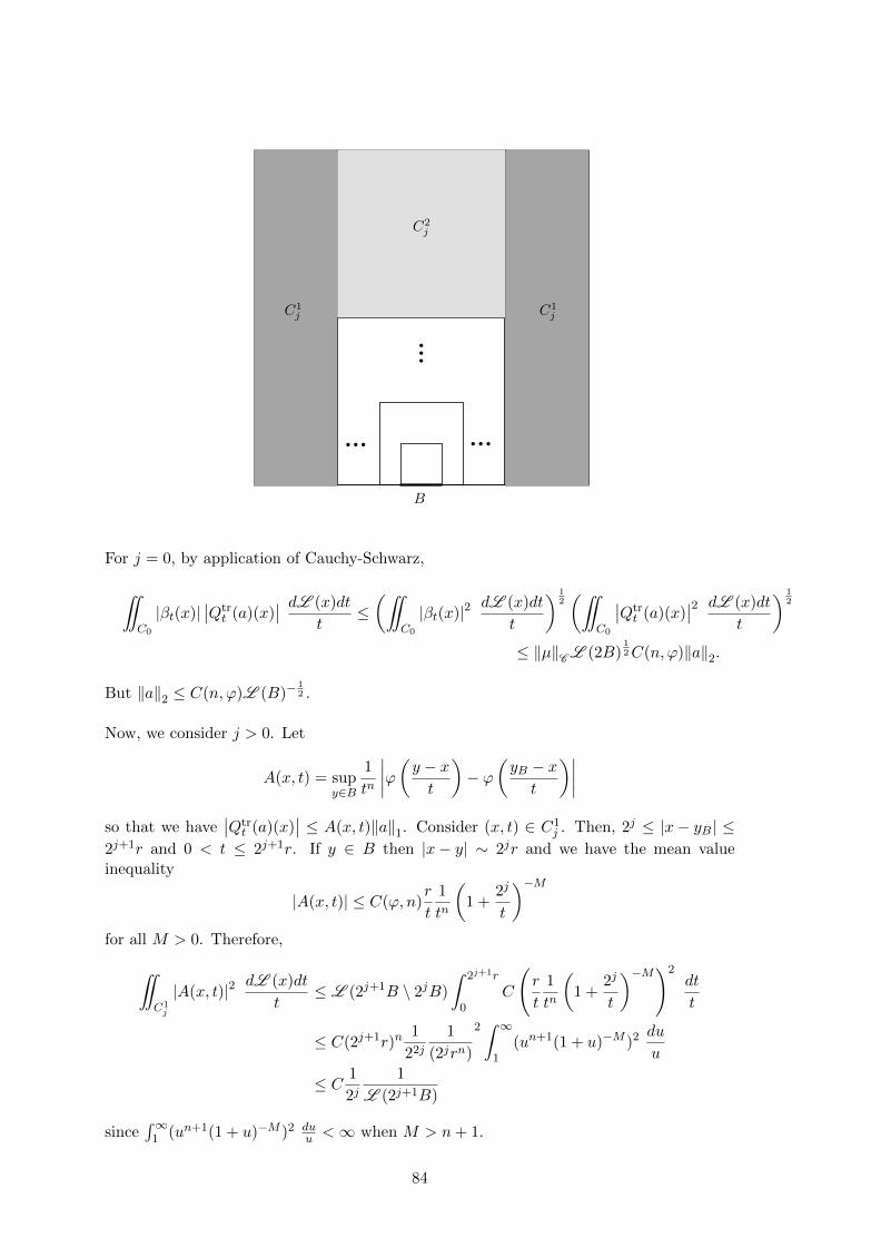
C2j

C1jC1

j

B

.........

For j = 0, by application of Cauchy-Schwarz,

¨C0

|βt(x)|∣∣Qtr

t (a)(x)∣∣ dL (x)dt

t≤(¨

C0

|βt(x)|2 dL (x)dt

t

) 12(¨

C0

∣∣Qtrt (a)(x)

∣∣2 dL (x)dt

t

) 12

≤ ‖µ‖C L (2B)12C(n, ϕ)‖a‖2.

But ‖a‖2 ≤ C(n, ϕ)L (B)−12 .

Now, we consider j > 0. Let

A(x, t) = supy∈B

1

tn

∣∣∣∣ϕ(y − xt)− ϕ

(yB − xt

)∣∣∣∣so that we have

∣∣Qtrt (a)(x)

∣∣ ≤ A(x, t)‖a‖1. Consider (x, t) ∈ C1j . Then, 2j ≤ |x− yB| ≤

2j+1r and 0 < t ≤ 2j+1r. If y ∈ B then |x− y| ∼ 2jr and we have the mean valueinequality

|A(x, t)| ≤ C(ϕ, n)r

t

1

tn

(1 +

2j

t

)−Mfor all M > 0. Therefore,

¨C1j

|A(x, t)|2 dL (x)dt

t≤ L (2j+1B \ 2jB)

ˆ 2j+1r

0C

(r

t

1

tn

(1 +

2j

t

)−M)2dt

t

≤ C(2j+1r)n1

22j

1

(2jrn)

2 ˆ ∞1

(un+1(1 + u)−M )2 du

u

≤ C 1

2j1

L (2j+1B)

since´∞

1 (un+1(1 + u)−M )2 duu <∞ when M > n+ 1.

84

Now, if (x, t) ∈ C2j , we have |x− yB| ≤ 2jr, and 2jr ≤ t < 2j+1r and the mean value

inequality takes the form

A(x, t) ≤ supz∈B

(r

t

1

tn

∣∣∣∣∇ϕ(z − xt)∣∣∣∣)

and when x ∈ 2B, (r

t

1

tn

∣∣∣∣∇ϕ(z − xt)∣∣∣∣) ≤ r

(2jr)n+1‖∇ϕ‖∞

and when x 6∈ 2B,

A(x, t) ≤ C(n)r

(2jr)n+1

(1 +|yB − x|

2jr

)−M.

Therefore,

¨C2j

|A(x, t)|2 dL (x)dt

t≤ˆ

2jB

ˆ 2j+1r

2jr|A(x, t)|2 dL (x)dt

t

≤ ln 2

ˆ2jB|A(x, t)|2 dL (x)

≤ ln 2

(ˆ2B|A(x, t)|2 dL (x) +

ˆ2jB\2B

|A(x, t)|2 dL (x)

)

≤ C

(1

2j(n+2)L (B)+

r2

(2jr)2(n+1)

ˆ2jB

(1 +|yB − x|

2jr

)−2M

dL (x)

)

≤ C(

1

22jL (B)+

1

22jL (2jB)

)Therefore, ¨

C2j

|A(x, t)|2 dL (x)dt

t≤ C

22j

1

L (2j+1B)

and

I =

¨Rn+1+

|βt(x)|∣∣Qtr

t (a)(x)∣∣ dL (x)dt

t

=∑j

¨Cj

|βt(x)|∣∣Qtr

t (a)(x)∣∣ dL (x)dt

t

≤∑j

(¨Cj

|βt(x)|2 dL (x)dt

t

) 12(¨

Cj

∣∣Qtrt (a)(x)

∣∣2 dL (x)dt

t

) 12

≤(‖µ‖C L (2j+1B)

) 12

(C

22j

1

L (2j+1B)

) 12

≤ C‖µ‖12C .

This tells us that limε→0, R→∞ Iε,R exists and

limε→0, R→∞

Iε,R =

¨Rn+1+

βt(x)Qtrt (a)(x)

dL (x)dt

t.

85

Now, take a general f ∈ H1. Then, we can find λj and aj ∈ A∞ such that f =∑

j λjajin H1 and in particular L1(Rn) and also such that

∑j |λj | ≤ 2‖f‖H1 . Using the fact that

Iε,R ≤ Cε,R‖f‖1, we can write

Iε,R(f) =∑j

λjIε,R(aj).

Therefore,

|Iε,R(f)| ≤∑j

|λj | |Iε,R(aj)| ≤ C‖µ‖12C

∑j

|λj | ≤ C‖µ‖12C 2‖f‖H1

with C independent of ε and R.

Let

bε,R =

ˆ R

εQtβt

dt

t

and note that it is a measurable function. Also, 〈bε,R, f〉 = Iε,R(f). Thus, bε,R ∈ BMO

with ‖bε,R‖∗ ≤ C‖µ‖12C with C independent of ε,R. Now since BMO = H1′ there exists

a convergent subsequence (bεj ,Rj ) and 〈bεj ,Rj , f〉 → 〈β, f〉 for some β ∈ BMO. Theuniqueness of β then follows from the uniqueness of limε→0, R→∞ Iε,R(a) for atoms a ∈ A∞

and then by the density of Vect A∞ in H1 so limε→0, R→∞〈bε,R, f〉 = 〈β, f〉.

Exercise 8.2.6. Replace Qtrt by Rt with kernel Kt satisfying:

Kt(x, y) ≤ C

tn

(1 +|x− y|t

)−n−εwhen ε > 0 and

|Kt(x, y)−Kt(x, z)| ≤ C(|y − z|t

)δ 1

tn

(1 +|x− y|t

)−n−ε−δfor δ > 0 when |y − z| ≤ 1

2(t+ |x− y|).

Theorem 8.2.7 (Paraproducts of J.M. Bony). Let ψ, ψ, ϕ ∈ S (Rn) such that´Rn ψ dL =´

Rn ψ dL = 0. Define,

Qt = ψt ∗ , Qt = ψt ∗ , Pt = ϕt ∗

and let b ∈ BMO. Let

πb(f) =

ˆ ∞0

Qt(Qt(b)Pt(f))dt

t.

Then,

(i) We have πb ∈ L(L2(Rn)) and

‖πb(f)‖2 ≤ C(n, ϕ, ψ, ψ)‖b‖∗‖f‖2

whenever f ∈ L2(Rn),

(ii) πb ∈ CZO1,

86

(iii) πtrb (1) = 0 in BMO,

(iv) If´Rn ϕ dL = 1 and ψ, ψ are radial functions satisfying

ˆ ∞0

ψ(tξ)ψ(tξ)dt

t= 1

then πb(1) = b in BMO.

Proof. (i) Let

Iε,R = 〈ˆ R

εQt(Qt(b)Pt(f))

dt

t, g〉

whenever g ∈ L2(Rn). Then, by noting that 〈Qt(Qt(b)Pt(f)), g〉 = 〈Qt(b)Pt(f), Qtrt (g)〉

and applying Fubini,

|Iε,R| =∣∣∣∣ˆ R

ε

ˆRnQt(b)(x)Pt(f)(x)Qtr

t (g)(x)dL (x)dt

t

∣∣∣∣≤ˆ R

ε

ˆRn

∣∣∣Qt(b)(x)Pt(f)(x)Qtrt (g)(x)

∣∣∣ dL (x)dt

t

≤ I1 I2

where

I21 =

¨Rn+1+

|Pt(f)(x)Qt(b)(x)|2 dL (x)dt

t

and

I22 =

¨Rn+1+

∣∣∣Qt(b)(x)Pt(f)(x)Qtrt (g)(x)

∣∣∣2 dL (x)dt

t.

We have the Littlewood Paley estimate I2 ≤ C(ψ, n)‖g‖2 since ψ ∈ S (Rn) and´Rn ψ dL = 0. Then, note that

|Qt(b)(x)|2 dL (x)dt

t

is a Carleson measure and so by application of Carleson Embedding Theorem withRt = Pt,

I1 ≤ C(n, ϕ, ψ)‖f‖2‖b‖∗.

Hence,

limε→0, R→∞

Iε,R =

¨Rn+1+

Qt(b)(x)Pt(f)(x)Qtrt (g)(x)

dL (x)dt

t

is a bounded bilinear form on L2(Rn) and we conclude (i) by invoking the RieszRepresentation Theorem.

(ii) Let f, g ∈ C∞c (Rn). Then,

〈πb(f), g〉 =

¨Rn+1+

Qt(b)(x)Pt(f)(x)Qtrt (g)(x)

dL (x)dt

t= 〈K, g ⊗ f〉

where g ⊗ f(y, z) = g(y)f(z) and

K(y, z) =

ˆ ∞0

ˆRnϕt(z − x)Qt(b)(x)ψt(y − x)

dL (x)dt

t

87

where this equality is in S (Rn)′.

Now by using the fact that |Qt(b)(x)| ≤ C‖b‖∗ and by the decay of ϕ, ψ using thatηε(x) ≤ (1 + |x|)−n−ε and ηε ∗ ηε ≤ C(n, ε)ηε, we have

ˆ ∞0

1

tnηε

(y − zt

)dt

t≤ C(n, ε)

|y − z|n.

The estimate for ∇yK follows since under differentiation in y, ψt gives an extra 1t

factor and so we get

|∇yK| ≤C(n, ε)

|y − z|n+1 .

So, K ∈ CZK1.

(iv) We already have that

〈πb(f), g〉 =

¨Rn+1+

Qt(b)(x)Pt(f)(x)Qtrt (g)(x)

dL (x)dt

t

whenever f, g ∈ L2(Rn). First, we show this same equality when f ∈ L∞(Rn) andwhen g = a ∈ A∞.

Recall that when b ∈ BMO and a ∈ A∞, we have

¨Rn+1+

|Qt(b)(x)|∣∣∣Qtr

t (a)(x)∣∣∣ dL (x)dt

t≤ C‖b‖∗.

Also, |Pt(f)(x)| ≤ ‖ϕ‖1‖f‖∞ for all (x, t) ∈ Rn+1+ . Therefore,

¨Rn+1+

Qt(b)(x)Pt(f)(x)Qtrt (a)(x)

dL (x)dt

t

exists.

Note that πtrb : H1 → L1(Rn) and so πtr

b (a) ∈ L1(Rn) and hence 〈f,πtrb (a)〉 well

defined and by definition 〈f,πtrb (a)〉 = 〈πb(f), a〉. Let fk = fχ[−2k,2k]n when k ∈ N

and so fk ∈ L2 ∩ L∞(Rn). So by Dominated convergence 〈fk,πtrb (a)〉 → 〈f,πtr

b (a)〉and Pt(fk)(x)→ Pt(f)(x) for all (x, t) ∈ Rn+1

+ .

Now, set f = 1, and since we assumed that´Rn ϕ dL = 1, we have Pt(1) = 1 for all

(x, t) ∈ Rn+1+ . Then,

〈πb(1), a〉 =

¨Rn+1+

Qt(b)(x)Qtrt (a)

dL (x)dt

t

= limε→0, R→∞

ˆ R

ε

ˆRnQt(b)(x)Qtr

t (a)dL (x)dt

t= lim

ε→0, R→∞〈b, Uε,R〉

where

Uε,R =

ˆ R

εQtrt Q

trt (a)

dt

t.

It suffices to prove that Uε,R → a in H1 since this gives 〈πb(1), a〉 = 〈b, a〉 for alla ∈ A∞ and hence πb(1) = b.

88

We note that a ∈ L2(Rn) since spt a ⊂ B for some ball B and ‖a‖∞ ≤ L (B)−1.Using the assumption that ψ, ψ are radial, we have

Uε,R(a)(ξ) =

ˆ R

εψ(tξ)

ˆψ(tξ)

dt

ta(ξ)

and so Uε,R(a)→ a in L2(Rn).

Define a function ϕ on Rn by

ϕ(ξ) =

ˆ ∞1

ψ(tξ)ˆψ(tξ)

dt

t= 1−

ˆ 1

0ψ(tξ)

ˆψ(tξ)

dt

t

whenever ξ ∈ Rn \ 0. It is an easy fact that ϕ ∈ C∞(Rn \ 0), with decay at ∞.Then, ϕ extends to a C∞(Rn) function with ϕ(0) = 1. This implies that ϕ ∈ S (Rn)

and so ϕ ∈ S (Rn). Then, Uε,R(a)(ξ) = (−ϕ(Rξ) + ϕ(εξ))a(ξ) so that

Uε,R = ϕR ∗ a+ ϕε ∗ a.

Then, it is enough to prove that ϕR ∗ a → a in H1 as R → ∞ and ϕε ∗ a → a inH1 as ε→ 0.

Now, using´Rn a = 0, spt a ⊂ B = B(xB, rB) and ‖a‖1 ≤ 1, we leave it as an

exercise to show that

|ϕR ∗ a(x)| ≤ C(n, ϕ)

R

(1

Rn

(1 +|x− xB|−n−1

R

))when R is large, ˆ

RnϕR ∗ a =

ˆRnϕR

ˆRna = 0

andR

C(n, ϕ)ϕR ∗ a ∈ H1

with uniform norm with respect to R (ie., ‖ϕR ∗ a‖H1 = O( 1R)).

Set hε = ϕε ∗ a − a. Then, we know that hε → 0 in L2(Rn). Define functionsh1ε = (hε −m2B hε)χ2B and h2

ε by hε = h1ε + h2

ε. Then, spt h1ε ⊂ 2B,

ˆ2B

∣∣h1ε

∣∣2 dL ≤ˆ

2B|hε|2 dL → 0

and´

2B h1ε dL = 0. These facts then imply that h1

ε → 0 in H1 using the fact thatf ∈ L2(Rn) : spt f ⊂ 2B

continuously embeds into H1. Also,

ˆRnh2ε =

ˆRnhε −

ˆRnh1ε = 0− 0 = 0.

We leave it as an exercise to show that∣∣h2ε(x)

∣∣ ≤ C(n, ϕ)C(ε)(1 + |x− xB|)−n−1

for all x ∈ Rn and ε < rB where

C(ε) = sup(m2B hε, ε).

With this fact in hand, ‖hε‖H1 ≤ C(n, ϕ)C(ε)→ 0.

89

(iii) We note that as before,

〈πtrb (f), g〉 =

¨Rn+1+

Qt(b)(x)Pt(g)(x)Qtrt (f)(x)

dL (x)dt

t

for all f, g ∈ L2(Rn). We want to show that this holds when we have f ∈ L∞(Rn)and g ∈ A∞. As before, let fk = f[−2k,2k]n , and so

〈πtrb (f), g〉 = 〈f,πb(g)〉

= limk→∞〈fk,πb(g)〉

=

¨Rn+1+

Qt(b)(x)Pt(g)(x)Qtrt (fk)(x)

dL (x)dt

t

Now, although Qtrt (fk)(x) → Qtr

t (f)(x) for all (x, t) we cannot apply Dominatedconvergence theorem since

´Rn g 6= 0. Instead, cover Rn+1

+ by set Cj as in the proofof the Carleson Embedding Theorem 8.2.5.

For j > 0, we have the same estimates of P trt (g) as for for Qtr

t (g) in (iv). So,∣∣∣Qtrt (g)

∣∣∣ ≤ C uniformly with respect to t, x, k. Then, take the limit.

For the situation when j = 0,

∣∣∣∣¨C0

Qt(b)(x)Pt(g)(x)Qtrt (f − fk)(x)

dL (x)dt

t

∣∣∣∣ ≤ (¨C0

∣∣∣Qtrt (f − fk)(x)

∣∣∣2 dL (x)dt

t

) 12

(¨C0

|Qt(b)(x)Pt(g)(x)|2 dL (x)dt

t

) 12

If k is large, f − fk = 0 on a neighbourhood of 2B. The region C0 is above 2B, sowe can apply decay estimates to prove

¨C0

∣∣∣Qtrt (f − fk)(x)

∣∣∣2 dL (x)dt

t→ 0.

The other term is dealt with by noting that |Qt(b)(x)|2 dL (x)dtt is a Carleson measure.

Now, put f = 1, Qtrt (1)(x) = 0 for all (x, t) ∈ Rn+1

+ since´Rn ψ dL = 0.Thus,

〈πtrb (1), g〉 = 0 for all g ∈ A∞ and so πtr

b (1) = 0 in BMO.

90

Chapter 9

Littlewood Paley Estimates

Definition 9.0.8 (Littlewood Paley Estimate). Let (Rt)t>0 be a family of operators on aHilbert space. Suppose there exists a C > 0 such that

ˆ ∞0‖Rtf‖

dt

t≤ C‖f‖2. (LPE)

Such an estimate is called a Littlewood Paley Estimate.

Example 9.0.9. Let Rt = ψt ∗ where ψ ∈ S (Rn) with´Rn ψ dL = 0. Then,

ˆ ∞0‖Rtf‖22

dt

t= C

ˆRn

(ˆ ∞0

∣∣∣ψ(tξ)∣∣∣2 dt

t

) ∣∣∣f(ξ)∣∣∣2 dL (ξ) ≤ C(ψ)‖f‖22.

Remark 9.0.10. Unlike in the example, we will not have the luxury of the Fourier Trans-form in the general theory. This is our goal.

Definition 9.0.11 (Operator ε-family). Let ε > 0 and (Rt)t>0 be a family of Operatorswith kernels Kt(x, y) where the map (t, x, y) 7→ Kt(x, y) is measurable satisfying:

(i) For all (t, x, y, z) ∈ R+ × R3n,

|Kt(x, y)| ≤ C

tn

(1 +|x− y|t

)−n−ε,

(ii) For δ > 0,

|Kt(x, y)−Kt(x, z)| ≤ C(|y − z|t

)δ 1

tn

(1 +|x− y|t

)−n−ε−δ,

where C <∞. Such a family of operators is called an ε-family.

Theorem 9.0.12 (Christ, Journe, Coifman, Meyer). Let (Rt)t>0 be an ε-family. Then,

(i) LPE holds,

91

(ii) The measure

|Rt(1)(x)| dL (x)dt

t

is a Carleson measure,

are equivalent statements.

Remark 9.0.13. The direction (ii) implies (i) goes from one test function to all L2(Rn)functions.

The following proof of 9.0.12 is due to Fefferman-Stein.

Proof of 9.0.12 (i) =⇒ (ii). Fix a Carleson box R = B × (0, r] where r = radB and letf ∈ L∞(Rn). Let f1 = fχ2B and f2 = fχc2B so that f = f1 + f2. Then,

¨R|Rt(f1)(x)|2 dL (x)dt

t≤ C‖f1‖22 ≤ C‖f‖∞L (2B).

By noting that whenever (x, t) ∈ R implies x ∈ B, we have

|Rt(f2)(x)| =∣∣∣∣ˆy∈c2B

Kt(x, y)f(y) dL (y)

∣∣∣∣≤ ‖f‖∞

ˆy∈c2B

C

tn

(1 +|x− y|t

)−n−εdL (y) ≤ C‖f‖∞

(t

r

)εTherefore,

¨R|Rt(f2)(x)|2 dL (x)dt

t≤ C‖f‖2∞

¨R

(t

r

)2ε dL (x)dt

t≤ C‖f‖2∞L (B)

1

2ε.

Before we proceed to prove the converse, we require the following important Lemma.

Lemma 9.0.14. Let (Vt)t>0 be an ε-family. Suppose that Vt(1) = 0. Then, there exist anε′ ∈ (0, ε) and a C > 0 such that for all (t, s) ∈ (0,∞)2,

‖VtV ∗s ‖L(L2(Rn) ≤ Ch(s

t)

where h(x) = infx, 1

x

ε′.

Proof of 9.0.12 (ii) =⇒ (i). First, define Vt = Rt − Rt(1)Pt where Pt = ϕt ∗ , ϕ ∈C∞c (Rn) with

´Rn ϕ dL = 1. Then,

(Rt(1)Pt)f(x) = Rt(1)(x)Pt(f)(x) =

ˆRnRt(1)(x)ϕt(x− y)f(y) dL (y)

92

which shows that (Vt)t>0 is an ε-family with the same ε as Rt. Now, take f ∈ L2(Rn).Then, ¨

Rn+1+

|Rt(1)(x)Pt(f)(x)|2 dL (x)dt

t≤ C‖µ‖C ‖f‖

22

where

µ = |Rt(1)(x)|2 dL (x)dt

t.

Hence, (ii) implies that |Rt(1)(x)Pt(1)(x)|2 dL (x)dtt satisfies (i) and so proving (i) for Rt

reduces to proving (i) for Vt.

Firstly, we note that Vt(1)(x) = 0 for all (x, t) ∈ Rn+1+ . We use a technique developed for

a different purpose called the Cotlar-Knapp-Stein inequality or T ∗T -argument. We have

¨Rn+1+

|Vt(f)(x)|2 dL (x)dt

t=

ˆ ∞0〈Vtf, Vtf〉

dt

t=

ˆ ∞0〈V ∗t Vtf, f〉

dt

t

and for each t, V ∗t Vt is a bounded (from ε-family hypothesis) self-adjoint operator onL2(Rn). We want the right hand side to be equal to 〈Sf, f〉 for some bounded operator S.

Fix r,R such that 0 < r ≤ R <∞, and let

Sr,R =

ˆ R

rV ∗t Vt

dt

t

and it is a bounded operator on L2(Rn) since by the ε-family hypothesis ‖V ∗t Vt‖L(L2(Rn))

is uniformly bounded in t and so

‖Sr,R‖L(L2(Rn)) ≤ˆ R

r‖V ∗t Vt‖L(L2(Rn))

dt

t≤ C ln

(R

r

).

Also, Sr,R is self adjoint and therefore, operator theory tells us that

‖Sr,R‖mL(L2(Rn)) = ‖Smr,R‖L(L2(Rn)).

We write out Sm:

Smr,R =

ˆ R

r. . .

ˆ R

rV ∗t1(Vt1V

∗t2)Vt2 . . . (Vtn−1V

∗tm)Vtm

dt1t1

. . .dtmtm

.

and on application of Lemma 9.0.14, we get

‖Smr,R‖L(L2(Rn))

≤ˆ R

r. . .

ˆ R

r‖V ∗t1‖L(L2(Rn))

Ch

(t1t2

). . . Ch

(tn−1

tm

)‖Vtm‖L(L2(Rn))

dt1t1

. . .dtmtm

≤ Cm−1

ˆ R

r. . .

ˆ R

r‖V ∗t1‖L(L2(Rn))

h

(t1t2

). . . h

(tn−1

tm

)‖Vtm‖L(L2(Rn))

dt1t1

. . .dtmtm

.

Since the integral is a convolution, we have the technical estimate that

ˆ ∞0

h

(tj−1

tj

)h

(tjtj+1

)dtjtj

= Cε′h

(tj−1

tj+1

).

93

Combining this with the facts that ‖V ∗tj‖L(L2(Rn))∈ L∞(R+) and h( t1tm ) ∈ L1(R+,

dtt ), we

have

‖Smr,R‖L(L2(Rn))≤ Cm−1Cm−2

ε′

ˆ R

r

ˆ R

r‖V ∗t1‖L(L2(Rn))

h

(t1tm

)‖Vtm‖L(L2(Rn))

dt1t1

dtmtm

≤ Cm−1Cm−2ε′ C

ˆ R

r‖Vtm‖L(L2(Rn))

dtmtm

≤ C ′′(CCε)m ln

(R

r

)and

‖Sr,R‖L(L2(Rn)) ≤ lim infm→∞

(C ′′(CCε)

m ln

(R

r

)) 1m

≤ CCε′ .

Then, we find that

limr→0, R→∞

∣∣∣∣ˆ R

rV ∗t Vt

dt

t

∣∣∣∣ ≤ CCε′which proves

ˆ ∞0‖Vtf‖22

dt

t= lim

r→0, R→∞

ˆ R

r〈V ∗t Vt, f〉

dt

t≤ CCε′‖f‖22

for all f ∈ L2(Rn).

Now, we return to the proof of the Lemma.

Proof of Lemma 9.0.14. We study VtV∗s and its kernel. Let Vt(x, y) and V ∗s (x, y) denote

the kernels of Vt and V ∗s respectively and

VtV∗s (f)(x) =

ˆRnVt(x, z)

ˆRnV ∗s (z, y)f(y) dL (y)dL (z) =

ˆRnKs,t(x, y)f(y) dL (y)

where

Ks,t(x, y) =

ˆRnVt(x, z)Vs(y, z) dL (z).

We note that by Fubini, this expression holds for all f ∈ ∪1≤p≤∞Lp(Rn).

Now, assume that 0 < s < t. Then we have the estimates

|Vt(x, z)| ≤C

tn

(1 +|x− z|t

)−n−εand |Vs(x, z)| ≤

C

sn

(1 +|x− z|s

)−n−ε.

We leave it as an exercise to prove

ˆRn

C

tn

(1 +|x− z|t

)−n−ε Csn

(1 +|x− z|s

)−n−εdL (z)

≤ C(n, ε)C

tn

(1 +|x− y|t

)−n−εfor 0 < s ≤ t.

94

Now, using oscillation of y 7→ Vs(y, z), we can write

Ks,t(x, y) =

ˆRn

(Vt(x, z)− Vt(x, y))Vs(y, z) dL (z)

and hence

|Ks,t(x, y)| ≤ˆRn|Vt(x, z)− Vt(x, y)| |Vs(y, z)| dL (z).

We also have

|Vt(x, z)− Vt(x, y)| ≤

Ctn (decay)

Ctn

(|y−z|t

)δ(regularity in y)

and this implies that for all δ′ ∈ (0, δ), and some C ′ > 0,

|Vt(x, z)− Vt(x, y)| ≤ C ′

tn

(|y − z|t

)δ′.

Therefore, by choosing 0 < δ′ < ε,

|Ks,t(x, y)| ≤ C ′

tn

ˆRn

(|y − z|t

)δ′ (1 +|y − z|t

)−n−εdL (z) ≤ C

tnδδ′

tδ′.

The technical estimate gives us

|Ks,t(x, y)| ≤ C

tn

(1 +|x− y|t

)−n−ε.

Now, if X ≤ A and X ≤ B, then for all θ ∈ [0, 1] the estimate X ≤ AθB1−θ holds. Weapply this to |Ks,t(x, y)| with θ such that (1− θ)(n+ ε) = n+ ν > n to obtain

|Ks,t(x, y)| ≤ C(st

)δ′θ (1 +|y − z|t

)−n−νfor all 0 < s ≤ t. By symmetry,

|Ks,t(x, y)| ≤ C(t

s

)δ′θ (1 +|y − z|t

)−n−ν.

Thus we have

supx∈Rn

ˆRn|Ks,t(x, y)| ≤ C ′′ inf

(s

t,t

s

)δ′θand sup

y∈Rn

ˆRn|Ks,t(x, y)| ≤ C ′′ inf

(s

t,t

s

)δ′θwhich gives

‖VtV ∗s ‖L(L1(Rn)) ≤ inf

(s

t,t

s

)δ′θand ‖VtV ∗s ‖L(L∞(Rn)) ≤ C

′′ inf

(s

t,t

s

)δ′θ.

Then interpolation yields

‖VtV ∗s ‖L(L2(Rn)) ≤ C inf

(s

t,t

s

)δ′θ.

95

Chapter 10

T (1) Theorem for SingularIntegrals

This chapter concerns itself with the question of proving the boundedness of L2(Rn) op-erators that are associated to Calderon-Zygmund kernels.

Definition 10.0.15 (Schwartz kernel). Let T : C∞c (Rn)→ C∞c (Rn) be linear and contin-uous. Then, the uniquely given K ∈ C∞c (R2n)′ defined by

〈K, g ⊗ f〉 = 〈Tf, g〉

is called the Schwartz kernel of T .

We begin with the following definition.

Definition 10.0.16 (Singular integral operator). Let T : C∞c (Rn) → C∞c (Rn)′ be linearand continuous. Then T is said to be a Singular integral operator if its Schwartz kernelwhen restricted to c∆ is a CZKα for some α > 0. We write T ∈ SIO.

We emphasise that while a Singular integral operator has CZK kernel, it is not a Calderon-Zygmund operator. Recall that a Calderon-Zygmund operator is bounded on L2(Rn). Thefollowing examples emphasise that a Singular integral operator need not be bounded onL2(Rn).

Example 10.0.17. (i) Tf(x) = |x|2 f(x) when x ∈ Rn is not bounded. But T is an SIOand the Schwartz kernel is given by K(x, y) = |x|2 δ0(x− y) and K|c∆ = 0 ∈ CZKα.

(ii) Tf = f ′ whenever f ∈ C∞c (Rn) is not bounded on L2(Rn). The Schwartz kernel hereis given by K(x, y) = −δ′0(x− y). Again, K|c∆ = 0 ∈ CZK

(iii) Tf(x) = ln |x| f(x) when f is measurable. Then, T |C∞c (Rn) ∈ SIO but ln |x| 6∈L∞(Rn). So, it is not bounded on L2(Rn). It will be useful to emphasise for thesequel that that T (1) = ln |x| ∈ BMO.

The previous examples illustrated that one of the problem for the boundedness of a T ∈SIO on L2(Rn) is the behaviour of the Schwartz kernel on the diagonal ∆. We will prove

96

a theorem that T ∈ SIO is bounded in L2(Rn) if and only if both T (1), T tr(1) ∈ BMOand when T has the “weak boundedness property.” In the sequel, we will give a rigorousformulation of this property. This is the key property that will give control on the diagonalof the Schwartz kernel of T .

Definition 10.0.18 (NB,q). For q ∈ N and B a ball in Rn and any ϕ ∈ C∞c (Rn) withspt ϕ ⊂ B, define

NB,q(ϕ) = supα∈Nn, |α|≤q

(‖∂αϕ‖∞(radB)|α|

).

Remark 10.0.19. This is a scale invariant quantity. Let spt ϕ ⊂ B(0, 1) and

ψ(x) = ϕ

(x− x0

r

)for some x0 ∈ Rn and r > 0. Then, spt ψ ⊂ B(x0, r) and NB(x0,r),q(ψ) = NB(0,1),q(ϕ).

Proposition 10.0.20. Let T ∈ SIO and fix x0 ∈ Rn, r > 0 and define Tx0,r by

〈Tx0,rϕ,ψ〉 = 〈Tϕ(· −x0

r

), ψ

(· −x0

r

)〉.

Then, Tx0,r ∈ SIO and its kernel is given by Kx0,r(x, y) = rnK(rx+ x0, ry + x0).

Proof. Exercise.

Corollary 10.0.21. T ∈ L(L2(Rn)) if and only if Tx0,r ∈ L(L2(Rn)) and ‖Tx0,r‖L(L2(Rn)) ≤rn‖T‖L(L2(Rn)).

Definition 10.0.22 (Weak boundedness property). Let T ∈ SIO. We say that T has theweak boundedness property (or WBP) if there exists a q ∈ N, q > 0, and a C > 0 suchthat for all balls B and all ϕ,ψ ∈ C∞c (B),

|〈Tϕ, ψ〉| ≤ CL (B)NB,q(ϕ)NB,q(ψ).

Remark 10.0.23. We note that ‖ϕ‖2 ≤ L (B)12 ‖ϕ‖∞ ≤ L (B)

12NB,q(ϕ). Therefore, if

T ∈ L(L2(Rn)), then

|〈Tϕ, ψ〉| ≤ ‖T‖L(L2(Rn))‖ϕ‖2‖ψ‖2 ≤ ‖T‖L(L2(Rn))L (B)NB,q(ϕ)NB,q(ψ).

We now deal with the issue of giving meaning to T acting on the constant function f ≡1. Note that this is non trivial since T is an operator defined on compactly supportedfunctions.

Definition 10.0.24. Define

D0(Rn) =

ψ ∈ C∞c (Rn) :

ˆRnψ dL = 0

.

Lemma 10.0.25. Let T ∈ SIO and ψ ∈ D0(Rn). Let B be a ball such that spt ψ ⊂ B.Then, Tψ ∈ L1(c2B) and

‖Tψ‖L1(c2B) ≤ ‖K‖CZKαC(n,B)‖ψ‖L1(B).

97

Remark 10.0.26. In writing Tψ ∈ L1(c2B), we mean the distribution Tψ|c2B ∈ L1(c2B).

Proof. Fix ϕ ∈ C∞c (Rn) and spt ϕ ⊂ c2B. Then,

〈Tψ, ϕ〉 = 〈K,ϕ⊗ ψ〉 = 〈K|c∆ , ϕ⊗ ψ〉

since spt ϕ⊗ ψ ⊂ c∆. Certainly,

〈K|c∆ , ϕ⊗ψ〉 =

¨c∆K(x, y)ϕ(x)ψ(y) dL (y)dL (x) =

ˆRn

(ˆRnK(x, y)ψ(y) dL (y)

)ϕ(x) dL (x)

and so Tψ|c2B agrees with ˆRnK(x, y)ψ(y) dL (y).

Now, since´Rn ψ dL = 0,

ˆRnK(x, y)ψ(y) dL (y) =

ˆRn

(K(x, y)−K(x, yB))ψ(y) dL (y)

where yB is the centre of B and∣∣∣∣ˆRnK(x, y)ψ(y) dL (y)

∣∣∣∣ ≤ ‖K‖CZKα

ˆRn

(radB)α

|x− yB|n+α |ψ(y)| dL (y)

≤ ‖K‖CZKα

(radB)α

|x− yB|n+α ‖ψ‖L1(B).

The conclusion is achieved by integrating over x ∈ c2B.

Proposition 10.0.27. Let f ∈ C∞ ∩ L∞(Rn) and ψ ∈ D0(Rn) and let B be a ball suchthat spt ψ ⊂ B. Then, whenever η ∈ C∞c (Rn) such that spt η ⊂ 4B and η ≡ 1 on 3B,

〈T (fη), ψ〉+

ˆRn

(1− η)(x)f(x)T tr(ψ)(x) dL (x)

is well defined and does not depend on the choice of η.

Proof. We note that ψ and fη ∈ C∞c (Rn) and this implies that 〈T (fη), ψ〉 exists. By theapplication of Lemma 10.0.25, we have T tr(ψ)|c2B ∈ L1(c2B). Also, (1 − η)f ∈ L∞(Rn)and spt (1− η)f ⊂ c2B.

To show the independence of η, choose η1 and η2 with the desired properties. Then, wenote that

〈T (fη1), ψ〉+

ˆRn

(1− η1)(x)f(x)T tr(ψ)(x) dL (x)

= 〈T (fη2), ψ〉+

ˆRn

(1− η2)(x)f(x)T tr(ψ)(x) dL (x)

is equivalent to

〈T (f(η1 − η2)), ψ〉 =

ˆRn

(η1 − η2)(x)f(x)T tr(ψ)(x) dL (x).

98

Noting that spt ψ ⊂ B and spt (η1 − η2)f ⊂ 4B \ 3B, we compute

〈T (f(η1 − η2)), ψ〉 =

¨RnK(x, y)f(y)(η1 − η2)(x)ψ(x) dL (x)dL (y)

=

ˆRn

(η1 − η2)(x)f(x)

(ˆRnK(y, x)ψ(y) dL (y)

)dL (x)

by the application of Fubini.

As a consequence, we are able to make the following definition.

Definition 10.0.28. Whenever f ∈ C∞ ∩ L∞(Rn), define Tf by

〈Tf, ψ〉 = 〈T (fη), ψ〉+

ˆRn

(1− η)(x)f(x)T tr(ψ)(x) dL (x)

whenever ψ ∈ D0(Rn) and η ∈ C∞c (Rn) such that spt η ⊂ 4B and η ≡ 1 on 3B.

Proposition 10.0.29. Whenever f ∈ C∞ ∩ L∞(Rn), we have Tf ∈ D0(Rn)′.

Proof. We want to show that Tf ∈ D0(Rn)′ with bounds depending only on f . Let B bea ball and ψ ∈ D0(Rn) a such that spt ψ ⊂ B. Fix an η as in the definition of Tf .

As T ∈ L(C∞c (Rn),C∞c (Rn)′), there exists an integer M > 0 such that

|〈T (fη), ψ〉| ≤ C(M, 4B) sup|α|≤M

‖∂α(fη)‖∞ sup|α|≤M

‖∂αψ‖∞

≤ C ′(M, 4B) sup|α|≤M

‖∂αf‖L∞(B) sup|α|≤M

‖∂αψ‖∞

Now,

ˆRn

∣∣(1− η)(x)f(x)T tr(ψ)(x)∣∣ dL (x) ≤

ˆc2B‖1− η‖∞‖f‖∞

∣∣T tr(ψ)(x)∣∣ dL (x)

≤ ‖1− η‖∞‖f‖∞C(n, α)‖K‖CZKα‖ψ‖1

≤ C(n, α)(1 + ‖η‖∞)‖f‖∞‖K‖CZKα‖ψ‖∞L (B).

Altogether, we have shown

|〈Tf, ψ〉| ≤ C(M,B) sup|α|≤M

‖∂αψ‖∞.

This shows that ψ 7→ 〈Tf, ψ〉 is continuous on D0(Rn).

We now present the crucial theorem of this chapter.

Theorem 10.0.30 (T (1) Theorem of David-Journe (’84)). Let T ∈ SIO. Then, T ∈L(L2(Rn)) if and only if T possesses the weak boundedness property, T (1), T tr(1) ∈ BMO.

99

Remark 10.0.31. When we write T ∈ L(L2(Rn)), we mean T extends to such an operatorsince what we prove is that

|〈Tf, g〉| ≤ ‖f‖2‖g‖2whenever f, g ∈ C∞c (Rn).

The following Lemma is of use in the proof of the T (1) Theorem. We leave its proof as anexercise.

Lemma 10.0.32. Let ϕ ∈ C∞c (Rn) be a radial function such that´Rn ϕ dL = 1, and

spt ϕ ⊂ B(0, 12). Let Pt = ϕt ∗ . Then for all f ∈ C∞c (Rn),

limt→0

P 2t (f) = f and lim

t→∞P 2t (f) = 0

in C∞c (Rn).

Proof of the T (1) Theorem. We already have one direction: if T ∈ L(L2(Rn)) we havealready seen that T has WBP and T (1), T tr(1) ∈ BMO. We prove the converse.

Let T0 = T − πT (1) − πtrT tr(1) where πb is the paraproduct with b ∈ BMO. We note

we can choose πb such that πb ∈ CZO1 ⊂ SIO, πb(1) = b in BMO and πtrb = 0 in

BMO. Therefore, T0 ∈ SIO and possesses WBP. Also, T0(1) = T (1) − T (1) − 0 = 0and T tr

0 (1) = T tr(1) − 0 − T tr(1) = 0 in BMO. Since T ∈ L(L2(Rn)) if and only ifT0 ∈ L(L2(Rn)), we can assume that T (1) = 0 and T tr(1) = 0 in BMO.

Take a ϕ and Pt as in the hypothesis of Lemma 10.0.32. Fix f, g ∈ C∞c (Rn) and by thesame Lemma,

〈Tf, g〉 = limε→0〈TP 2

ε f, P2ε g〉 − lim

R→∞〈TP 2

Rf, P2Rg〉 = lim

ε→0

(〈TP 2

ε f, P2ε g〉 − 〈TP 2

1ε

f, P 21ε

g〉).

Also, the map t ∈ (0,∞) 7→ P 2t f ∈ C∞c (Rn) is C1 and therefore,

〈Tf, g〉 = limε→0

ˆ 1ε

ε

d

dt〈TP 2

t , P2t g〉 dt.

Here,d

dt〈TP 2

t , P2t g〉 dt = 〈T

(d

dtP 2t f

), P 2

t g〉+ 〈TP 2t f,

d

dtP 2t g〉

and since 〈TP 2t f,

ddtP

2t g〉 = 〈T tr

(ddtP

2t g), P 2

t f〉, it is enough to just treat 〈T(ddtP

2t f), P 2

t g〉.

Now, we note that P 2t f ∈ C∞c (Rn) ⊂ S (Rn) and we consider the spatial Fourier Trans-

form. On noting that ϕ is radial if and only if ϕ is radial, we have

d

dtP 2t f(ξ) =

d

dtP 2t f(ξ) =

d

dtϕ(tξ)2f(ξ) = 2

n∑k=1

ξk(∂kϕ(tξ))ϕ(tξ).

So define ψk(x) = −xkϕ(x) and ψk(x) = ∂kϕ(x) so that ψk, ψk ∈ C∞c (B(0, 12)) with´

Rn ψk dL =´Rn ψk dL = 0. Also,ψk(ξ) = ı∂kϕ(ξ) and

ˆψk(ξ) = −ıξkϕ(ξ) and therefore,

d

dtP 2t f(ξ) =

2

t

n∑k=1

t(ξk∂k ˆϕ(tξ)

)ϕ(tξ)f(ξ) =

2

t

n∑k=1

ψk(tξ)ˆψk(tξ)f(ξ).

100

Letting Qk,t = ψk,t ∗ and Qk,t = ψk,t ∗ we have

d

dtP 2t f =

2

t

n∑k=1

Qk,tQk,tf.

We consider Qk,tQk,tf for each k. So fix k and ε > 0. We prove that there exists a C > 0(independent of ε) such that∣∣∣∣∣

ˆ 1ε

ε〈TQk,tQk,tf, P 2

t g〉dt

t

∣∣∣∣∣ ≤ C‖f‖2‖g‖2.Let

Iε =

ˆ 1ε

ε〈TQk,tQk,tf, P 2

t g〉dt

t=

ˆ 1ε

ε〈Qtr

k,tTtrP 2

t g, Qk,tg〉dt

t.

and Rk,t = Qtrk,tT

trP 2t . Then, by Cauchy-Schwarz

|Iε| ≤

(ˆ 1ε

ε‖Rk,tg‖22

dt

t

) 12(ˆ 1

ε

ε‖Qk,tf‖

2

2

dt

t

) 12

.

By an LPE estimate, we get that(ˆ 1ε

ε‖Qk,tf‖

2

2

dt

t

) 12

≤ C(ψk)‖f‖2

and so it is enough to show that

ˆ ∞0‖Rk,tg‖22

dt

t≤ C(ϕ,ψk, T )‖g‖22.

We examine the kernel of Rk,t. Pick a h ∈ C∞c (Rn). First, we note that 〈Rk,tg, h〉 =〈TQk,th, P 2

t g〉. For u, v ∈ Rn, set

ψuk,t(x) = ψk,t(x− u) and ϕvk,t(x) = ϕt(x− v)

so that

Qk,th =

ˆRnψuk,th(u) dL (u) and P 2

t g =

ˆRnϕvt g(v) dL (v).

Using the continuity of T : C∞c (Rn)→ C∞c (Rn)′, we can write

〈TQk,th, P 2t g〉 =

ˆRn

ˆRnh(u)〈Tψuk,t, ϕvt 〉g(v) dL (u)dL (v)

and so the kernel of Rk,t is Kk,t(u, v) = 〈Tψuk,t, ϕvt 〉.

We estimate Kk,t(u, v). First, suppose |u− v| ≤ 3t. then, spt ψuk,t ⊂ B(u, t2) and spt ϕvt ⊂B(v, t) and by setting B = B(v, 4t) we have that spt ψuk,t, spt ϕvt ⊂ B. By the fact that Thas WBP,

|Kk,t(u, v)| ≤ CL (B)NB,q(ψuk,t)NB,q(ϕvt )

101

and so

|Kk,t(u, v)| ≤ CC(n, ψk, ϕ)

tn.

Now, suppose |u− v| ≥ 3t. As before, we have spt ψuk,t ⊂ B(u, t2) and also´Rn ψ

uk,t dL = 0

which gives ∣∣Tψuk,t(x)∣∣ ≤ C‖K‖CZKα

tα

|x− u|n+α ‖ψuk,t‖1

where K is the kernel of T and when x 6∈ B(u, t). Now, spt ϕvt ⊂ B(v, t) ⊂ cB(u, t) and so∣∣〈Tψuk,t, ϕvt 〉∣∣ =

ˆRnTψuk,t(x)ϕvt (x) dL (x) ≤ C‖K‖CZKα

tα

|v − u|n+α ‖ψk‖1‖ϕ‖1

since ‖ψuk,t‖1 = ‖ψk,t‖1 = ‖ψk‖1 and ‖ϕt‖1 = ‖ϕ‖1.

Now, we consider the regularity of Kk,t(u, v) with respect to v. We note that v 7→ ϕvt ∈C∞c (Rn) is a C1 function and

∂vlϕvt = −1

t(∂lϕ)t and ∂vlKk,t(u, v) = −1

t〈Tψuk,t, (∂lϕ)vt )〉.

This gives

|∂vlKk,t(u, v)| ≤ C

tn+1

(1 +|u− v|t

)−n−ε.

So (Rt)t>0 is an ε′-family for some ε′ < ε.

We compute Rk,t(1). Choose η ∈ C∞c (Rn) with η ≡ 1 on B(u, 3t2 ) and spt η ⊂ B(u, 2t).

Then,

Rk,t(1)(u) =

ˆRnKk,t(u, v) dL (v)

=

ˆRn〈Tψuk,t, ϕvt 〉 dL (v)

=

ˆRn〈Tψuk,t, ηϕvt 〉 dL (v) +

ˆRn〈Tψuk,t, (1− η)ϕvt 〉 dL (v)

= 〈Tψuk,t,ˆRnηϕvt dL (v)〉+

ˆRn

(ˆRnTψuk,t(x)(1− η)(x)ϕvt (x) dL (x)

)dL (v).

First, we have ˆRnηϕvt dL (v) = η

in C∞c (Rn) so 〈Tψuk,t,´Rn ηϕ

vt dL (v)〉 = 〈Tψuk,t, η〉. Also, Tψuk,t ∈ L1(spt (1 − η)) in x,

(1− η) ∈ L∞(Rn) in x, ϕvt ∈ L1(Rn) in v and ϕvt ∈ L∞(Rn) in x. By Fubini coupled with´Rn ψ

vk,t dL (v) = 1

ˆRn

(ˆRnTψuk,t(x)(1− η)(x)ϕvt (x) dL (x)

)dL (v) =

ˆRnTψuk,t(x)(1− η)(x) dL (x).

By definition of T tr(1) and using T tr(1) = 0 in BMO,

Rk,t(1)(u) =

ˆRn

(ˆRnTψuk,t(x)(1− η)(x)dL (x)

)+ 〈Tψuk,t, η〉 = 〈T tr(1), ψuk,t〉 = 0.

102

Combining these facts, we have shown that Rk,t is an ε′-family with Rk,t(1) = 0 for all tand k. In particular

|Rk,t(1)(x)|2 dL (x)dt

t

is Carleson. Therefore, by Theorem 9.0.12,

ˆ ∞0‖Rk,tg‖22

dt

t≤ C‖g‖22

and the proof is complete.

Remark 10.0.33 (Avoiding the reduction to T (1) = T tr(1) = 0). We note that for allt > 0 and all u ∈ Rn the equality Rk,t(1)(u) = 〈T tr(1), ψuk,t〉 holds when T tr(1) ∈ BMO.

Going back again to the definition of 〈T tr(1), ψuk,t〉 and comparing with the definition of

Qk,t(Ttr(1))(u) when T tr(1) ∈ BMO (since Qk,t =

ˇψuk,t ∗ ), we can see that

〈T tr(1), ψuk,t〉 = Qk,t(Ttr(1))(u).

Thus, Rk,t(1) = Qk,t(Ttr(1)). As the Littlewood Paley estimates combined with the decay

of Qk,t and T tr(1) ∈ BMO imply that

∣∣Qk,t(T tr(1))(x)∣∣2 dL (x)dt

t

is a Carleson measure we can conclude by applying Theorem 9.0.12.

103

Bibliography

[Boa54] Ralph Boas, Entire functions, Elsevier, 1954.

[CR77] Weiss G. Coifman R., Extensions of hardy spaces and their use in analysis, Bull.Amer. Math. Soc. 83 (1977), no. 4, 569–645.

[Fed96] Herbert Federer, Geometric measure theory, Springer-Verlag Berlin, 1996.

[G.81] De Barra G., Measure and integration, New Age International Ltd., 1981.

[GC91] Evans L. Gariepy C., Measure theory and fine properties of functions, CRC PressInc., 1991.

[Mey92] Yves Meyer, Wavelets and operators, Cambridge University Press, 1992.

[Ste71a] E.M. Stein, Singular integrals and differentability properties of functions, Prince-ton University Press, 1971.

[Ste71b] Weiss G. Stein, E.M., Introduction to fourier analysis on euclidean spaces, Prince-ton University Press, 1971.

[Ste93] E. M. Stein, Harmonic analysis: real-variable methods, orthogonality, and os-cillatory integrals, Princeton Mathematical Series, vol. 43, Princeton UniversityPress, Princeton, NJ, 1993.

[Yos95] Kosaku Yosida, Functional analysis, Springer-Verlag, 1995.

104

Notation

A∞ The collection of all ∞-atoms.

A p The collection of all p-atoms.

A∞Q The collection of ∞-atoms on a cube Q.

A pQ The collection of p-atoms on a cube Q.

L(X) Bounded linear operators T : X → X.

L(X,Y ) Bounded linear operators T : X → Y .

BMOp The space of f ∈ Lploc with mQ |f −mQ f |p ≤ C.

C(µ)(x) The Carleson function associated with the Carleson measure µ.

Ckc (Rn) Functions f : Rn → C, k times differentiable and compactly supported.

cO Complement of the set O.

CZKα Calderon-Zygmund Kernels of order α.

CZKα(H1,H2) Hilbert valued Calderon-Zygmund kernels from H1 to H2.

CZOα Calderon-Zygmund operators of order α.

CZOα(H1,H2) Hilbert valued Calderon-Zygmund operators from L2(Rn; H1) to L2(Rn; H2).

δ0(x) Dirac mass at x

diamE Diameter of a set E in the metric sense.

dist(E,F ) Distance from E to F in the metric sense.

dist(x,E) Distance from a point x to E in the metric sense.

Q Collection of dyadic cubes.

D(Q) Dyadic subcubes of Q.

K Field either R or C.

ˆ The Fourier transform.

H(Ω) Holomorphic functions in Ω.

105

‖· ‖H1,p Norm on the hardy space H1,p.

H1,p The Hardy space built out of A p.

H1 The hardy space H1 equivalent with every H1,p.

χX Indicator function of the set X.

χX Indicator function on the set X.

C Topological interior of C.

L The Lebesgue measure

`(Q) Length of the dyadic cube Q.

Lploc(dµ) Locally Lp space of the measure µ.

Lp,∞ Weak Lp space.

Lp(Rn) The same as Lp(dL ).

Lp(dµ) Lp space over Rn with respect to dµ. Same as Lp(Rn, µ).

Lp(M,µ) Space of µ-measurable functions for which |f |p is integrable.

Lp(M,dµ) Same as Lp(M,µ).

M Maximal function Mµ,M′µ or MQµ .

M′µ Uncentred maximal function.

Mµ(ν) Maximal function (centred) of ν with respect to µ.

MQµ Dyadic maximal function.

M]f The sharp maximal function of f .

M∗f The non-tangential maximum function of f : Rn+1+ → C.

Mf Centred cubic maximal function.

mE The mean of f on the set E.

NB,q(ϕ) Scale invariant quantity with respect to q ∈ N, ball B and smooth ϕ with spt ϕ ⊂B.

‖· ‖p,∞ Weak Lp quasi-norm.

ν ∗ u Convolution of u with ν.

Qj,k The parent cube of Qj,k.

ϕt Function family 1tnϕ(tx).

R+n+ 1 The positive half plane Rn × (0,∞).

P(X) The power set of X.

106

p. v.K Principle value integral operator associated to K.

Qj,k Dyadic cube of level j with lower left corner 2−jk.

radB Radius of the ball B.

Rt An ε-family of operators.

D0(Rn) Smooth compactly supported functions with vanishing integral.

FM Measurable functions f : M → K.

supB3x Supremum over B containing x.

T tr Real transpose of T .

Vect A p The collection of finite linear combinations of p-atoms.

B(x, r) Ball centred at x and of radius r > 0.

d∞ Infinity metric.

dE Standard Euclidean metric.

f+ The set of points for which f is positive.

f− The set of points for which f is negative.

X ′ Dual space of the Banach space X.

M′f Uncentred cubic maximal function.

107

Index

T (1) Theorem, 99Calderon-Zygmund

Decomposition, 63Kernel, 55Operator, 56

Hormander kernel, 62

Besicovitch Covering Theorem, 6BMO, 35

BMOp, 42Properties, 35

Bounded Mean Oscillation, 35Bounded Overlap, 5

CarlesonEmbedding, 83Measure, 76Norm, 76Window, 76

Carleson’s Lemma, 78Cavalieri’s principle, 21Cone, 76Convergence modulo constant, 36

Dyadic cubes, 8Children, 8Maximal, 9Parent, 8Properties, 8Whitney Covering, 9

Fourier symbol, 69

Hardy spaceH1,p, 48H1, 51H1 − BMO duality, 52∞-atom, 48p-atom, 48Equivalence Theorem, 49Norm, 49

Hilbert Transform, 57Boundedness, 59

Hilbert valuedLp space, 71Calderon-Zygmund Operator, 72Calderon-Zygmund kernel, 71

InequalityFefferman-Stein, 44Good λ, 43Hardy-Littlewood Sobolev, 24John-Nirenberg, 39

Lebesgue Differentiation Theorem, 15Doubling measures, 18

Littlewood Paley Estimate, 91Littlewood-Paley, 71

Continuous time, 75Log convex, 29Lorentz space, 26

Marcinkiewicz Interpolation Theorem, 28Maximal function

Boundedness on Lp, 22Centred cubic, 42Dyadic, 19Dyadic on Rn, 20Hardy-Littlewood maximal function, 14Maximal Theorem, 14

Dyadic, 19Maximal theorem for doubling measures,

17Non-tangential, 77Sharp, 43Uncentred, 17Uncentred cubic, 42

Measure, 2Doubling, 17Lebesgue Measure, 3Space, 3

Mikhlin Multiplier Theorem, 69

Operatorε-family, 91Cauchy, 61

108

Fourier multiplier, 69Singular integral, 96

Paraproduct, 86Phragmen-Lindelof Lemma, 32

Riesz Transform, 59Riesz-Thorin Theorem, 32

Schur’s Lemma, 30Schwartz kernel, 96Stampacchia Theorem, 47Strong type, 27Strongly measurable, 71Sublinear operator, 27

Tchebitchev-Markov inequality, 27Tent

Ball, 77Cube, 77Open set, 77

Vitali Covering Lemma, 4

Weak Lp space, 26Weak boundedness property, 97Weak type, 27Whitney Covering

Dyadic cubes, 9Properties, 10

Metric space, 12

109