high order singular value decomposition for plant

HAL Id: hal-02385304https://hal.inria.fr/hal-02385304

Submitted on 29 Nov 2019

HAL is a multi-disciplinary open accessarchive for the deposit and dissemination of sci-entific research documents, whether they are pub-lished or not. The documents may come fromteaching and research institutions in France orabroad, or from public or private research centers.

L’archive ouverte pluridisciplinaire HAL, estdestinée au dépôt et à la diffusion de documentsscientifiques de niveau recherche, publiés ou non,émanant des établissements d’enseignement et derecherche français ou étrangers, des laboratoirespublics ou privés.

High Order Singular Value Decomposition for PlantBiodiversity Estimation

Alessandra Bernardi, Martina Iannacito, Duccio Rocchini

To cite this version:Alessandra Bernardi, Martina Iannacito, Duccio Rocchini. High Order Singular Value Decompositionfor Plant Biodiversity Estimation. Bollettino dell’Unione Matematica Italiana, Springer Verlag, 2021,�10.1007/s40574-021-00300-w�. �hal-02385304�

https://hal.inria.fr/hal-02385304

https://hal.archives-ouvertes.fr

HIGH ORDER SINGULAR VALUE DECOMPOSITION FOR PLANT

BIODIVERSITY ESTIMATION

ALESSANDRA BERNARDI?, MARTINA IANNACITO†, AND ‡DUCCIO ROCCHINI

Abstract. We propose a new method to estimate plant biodiversity with Renyi and Rao indexesthrough the so called High Order Singular Value Decomposition (HOSVD) of tensors. Starting fromNASA multispectral images we evaluate biodiversity and we compare original biodiversity estimateswith those realised via the HOSVD compression methods for big data. Our strategy turns out to beextremely powerful in terms of storage memory and precision of the outcome. The obtained resultsare so promising that we can support the efficiency of our method in the ecological framework.

1. Introduction

In order to face Earth changes in space and time, satellite imageries are nowadays being used toprovide timely information over the whole globe.

From this point of view, starting from the early ’70s, technological improvements in remote sen-sors led to a growth in the number and in the size of available data. For example to store a band ofthe entire Earth’s surface from the MODIS sensor with a low spectral resolution, 5600 m, we needaround 99 MB. Therefore for rasters with higher spectral, spatial or radiometric resolutions thememory request increases significantly. One may point out that 99 MB are not much, if comparedwith the features of modern machines. However the memory needed to process thousands of imagesmight represent a crucial issue. Moreover, in order to perform any index computation over theseimages, they should be loaded into the computer RAM, which usually has lower capacity and isoccupied also by the system application and by our computing script.Since the advent of big data, which include multispectral and hyperspectral images, improving stor-age and analytical techniques became fundamental. Mathematicians are facing this challenge to-gether with computer scientists, physicists and engineers (cf. e.g. [DLDMV00, VVM12, ADKM11,LC10, STG+19, BP94, BBK+16, BDHM17, GSR+14, SSV+05, BBCM11, BBC+19]). The usualstructure for storing multispectral images are tensors. For matrices approximation there exists anoptimal technique, called Singular Values Decomposition, SVD (cf. [Sch07, Ste93, Mir59, EY36]).One application of SVD is image compression (cf. e.g. [WBWJ15, JXP12, GVL96]). Since we needto store data in tensors, the generalisation of matrices, we will present High Order Singular ValueDecomposition (HOSVD) firstly introduced in [DLDMV00, VVM12], a generalisation to tensorsof SVD to tensors. There are various techniques to approximate tensors by taking advantage ofthe HOSVD, those that will be implemented in this paper are the so called Truncated HOSVD(T-HOSVD) and Sequentially Truncated HOSVD (ST-HOSVD). Even if only for some special casesHOSVD provides optimal results ([VNVM14, BDHR17, DOT18]), it is possible to present an esti-mate of the tensor approximation errors. Indeed the core of the present paper will be application ofT-HOSVD and ST-HOSVD techniques, their modern versions and the error made by using them.Indeed in the last section we will apply some possible HOSVD implementations to tensors in which

?Department of Mathematics, University of Trento, 38123 Povo (TN), Italy†Inria Bordeaux - Sud-Ouest, 200, avenue de la Vieille Tour, 33405 Talence, France‡Department of Biodiversity and Molecular Ecology, Fondazione Edmund Mach, Research and

Innovation Centre, 38010 S. Micehle all’Adige (TN), ItalyE-mail addresses: [email protected], [email protected], [email protected]: September 2019.

1

2 A. BERNARDI, M. IANNACITO, AND D. ROCCHINI

we stored RED and NIR bands. Next from the compressed tensors we get NDVI rasters and overthem we compute biodiversity indexes. So we will be able to compare our biodiversity estimationsfrom compressed data with those realised over original data.As far as we know, this is the first attempt to estimate biodiversity with the presented indexesfrom HOSVD compressed data. Moreover the obtained results are extremely promising, letting ussupport its efficiency in ecological framework.

2. Ecological background

One of the main component of Erath’s biosphere is biodiversity, which is in strict relationshipwith the planet status in space and time. Measuring biodiversity over wide spatial scales is difficultconcerning time, costs and logistical issues, e.g.: (i) the number of sampling units to be investigated,(ii) the choice of the sampling design, (iii) the need to clearly define the statistical population, (iv)the need for an operational definition of a species community, etc. (cf. [Chi07]). Hence, ecolog-ical proxies of species diversity are important for developing effective management strategies andconservation plans worldwide (cf. [RBC+10]). From this point of view, environmental heterogene-ity is considered to be one of the main factors associated to a high degree of biological diversitygiven that areas with higher environmental heterogeneity can host more species due to the greaternumber of available niches within them. Therefore, measuring heterogeneity from satellite imagesmight represent a powerful approach to gather information of diversity changes in space and timein an effective manner (cf. [ZFL+19]). Nowadays, the advent of satellites has made possible havingreal images of a territory, even with a remarkable quality. This approach is behind the the remotesensing discipline. Many definitions have been proposed during the years for this subject. We referto the one presented in [CW11, p.6].

Definition 2.1. Remote sensing is the practice of deriving information about Earth’s land andwater surfaces using images acquired from an overhead perspective, using electromagnetic radiationin one or more regions of the electromagnetic spectrum, reflected or emitted from the Earth’ssurface.

This field of study is based on a well known physical phenomenon: different materials anddifferent organisms absorb and reflect electromagnetic radiations differently. Most of the modernsatellite sensors can acquire multiple images, divided in the so called bands.

Definition 2.2. Bands or channels are the recorded spectral measurements.

Depending on the sensor features, we can acquire images dived into the different bands.

Definition 2.3. Multi-spectral sensor can acquire from 4 up to 10 bands. Hyper-spectral sensorcan acquire more than 100 bands.

Data used in the present paper come from the MODerate-Resolution Imaging Spectroradiometersensor, or MODIS, built on both the satellites Terra and Aqua, cf. [CJ]. MODIS measures 36bands in the visible and infrared spectrum, at different resolutions. Firstly there are RED andNIR bands with pixel size of 250km and next 5 bands, still with RED and NIR, at 500m of spatialresolution. These are extremely useful for land observation. The remaining bands with 1km ofresolution consist of monitoring images from visible spectrum, MIR, NIR and TIR. The data areregistered four times a day: twice daytime and twice night-time. Images usually include the entireEarth’s surface.From the 60s the scientific community highlighted two important relations between spectral mea-surements and biomass:

• a direct relation between NIR region and biomass, i.e. greater the biomass greater the NIRreflected radiation measured and vice versa;

HIGH ORDER SINGULAR VALUE DECOMPOSITION FOR PLANT BIODIVERSITY ESTIMATION 3

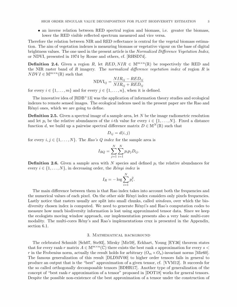
• an inverse relation between RED spectral region and biomass, i.e. greater the biomass,lower the RED visible reflected spectrum measured and vice versa.

Therefore the relation between NIR and RED reflectance is central for the vegetal biomass estima-tion. The aim of vegetation indexes is measuring biomass or vegetative vigour on the base of digitalbrightness values. The one used in the present article is the Normalized Difference Vegetation Index,or NDVI, presented in 1974 by Rouse and others, cf. [RHSD74].

Definition 2.4. Given a region R, let RED,NIR ∈ Mm×n(R) be respectively the RED andthe NIR raster band of R imagery. The normalized difference vegetation index of region R isNDV I ∈Mm×n(R) such that

NDVIij =NIRij −REDij

NIRij +REDij

for every i ∈ {1, . . . ,m} and for every j ∈ {1, . . . , n}, when it is defined.

The innovative idea of [RDB+13] was the application of information theory studies and ecologicalindexes to remote sensed images. The ecological indexes used in the present paper are the Rao andRenyi ones, which we are going to define.

Definition 2.5. Given a spectral image of a sample area, let N be the image radiometric resolutionand let pi be the relative abundances of the i-th value for every i ∈ {1, . . . , N}. Fixed a distancefunction d, we build up a pairwise spectral difference matrix D ∈MN (R) such that

Dij = d(i, j)

for every i, j ∈ {1, . . . , N}. The Rao’s Q index for the sample area is

IRQ =N∑j=1

N∑i=1

pipjDij .

Definition 2.6. Given a sample area with N species and defined pi the relative abundances forevery i ∈ {1, . . . , N}, in decreasing order, the Renyi index is

IR = − logN∑i=1

p2i .

The main difference between them is that Rao index takes into account both the frequencies andthe numerical values of each pixel. On the other side Renyi index considers only pixels frequencies.Lastly notice that rasters usually are split into small chunks, called windows, over which the bio-diversity chosen index is computed. We need to generate Renyi’s and Rao’s computation codes tomeasure how much biodiversity information is lost using approximated tensor data. Since we keepthe ecologists moving window approach, our implementation presents also a very basic multi-coremodality. The multi-cores Reny’s and Rao’s implementations crux is presented in the Appendix,section 6.1.

3. Mathematical background

The celebrated Schmidt [Sch07, Ste93], Mirsky [Mir59], Eckhart, Young [EY36] theorem statesthat for every rank-r matrix A ∈Mm×n(C) there exists the best rank s approximation for every s <r in the Frobenius norm, actually the result holds for arbitrary (Om×On)-invariant norms [Mir60].The famous generalization of this result [DLDMV00] to higher order tensors fails in general toproduce an output that is the “best” approximation of a given tensor, cf. [VVM12]. It succeeds forthe so called orthogonally decomposable tensors [BDHR17]. Another type of generalization of theconcept of “best rank-r approximation of a tensor” proposed in [DOT18] works for general tensors.Despite the possible non-existence of the best approximation of a tensor under the construction of


[DLDMV00], this technique turns out to be very convenient from the computational point of viewand it is possible to prove that the outcome is a “quasi-optimal solution. In this paper we willmainly use the technique popularized by L. De Lathauwer and J. Vandewalle in [DLDMV00], theso called High Order Singular Value Decomposition (HOSVD), we will study two types of errorsmade by the specific approximation, we will make a comparison among them and we will show thatthey will be small enough to have very precise results.

Here some basic mathematical preliminaries. The number field will always be the complex fieldof numbers C.

Definition 3.1. Let V be a linear subspace of the tensor space Cn1 ⊗ · · · ⊗ Cnd . If for everyi ∈ {1, . . . , d}, there exist a subspace Vi ⊆ Cni such that

V = V1 ⊗ · · · ⊗ Vd,then V is a separable tensor subspace of Cn1 ⊗ · · · ⊗ Cnd .

Remark that not every subspace of Cn1 ⊗ · · · ⊗ Cnd is separable. The structure of a separabletensor space has some consequences on its elements.

Definition 3.2. The multilinear rank of a tensor A ∈ Cn1⊗· · ·⊗Cnd is the d-uple (r1, . . . , rd) withthe property that ri is the minimal dimension of a subspace Vi ⊂ Cni such that A ∈ V1 ⊗ · · · ⊗ Vdfor every i ∈ {1, . . . , d}.

Let A ∈ Cn1 ⊗ · · · ⊗ Cnd be a tensor and let (r1, . . . , rd) ∈ Nd. We will discuss if there exists,and in case how to determine, a tensor M of multilinear rank lower or equal component-wise than(r1, . . . , rd) which minimizes the Frobenius norm of the tensor difference, i.e.

M = arg infmlrank(T )≤(r1,...,rd)

∥∥A− T∥∥ .This problem is also known as Low MultiLinear Rank Approximation (LMLRA). M. Ishteva and L.De Lathauwer firstly stated this problem and introduced this acronym, cf. [IAVHDL11]. Lookingfor a tensor M ∈ Cn1 ⊗ · · · ⊗Cnd satisfying the stated rank properties means searching a subspaceVi ⊂ Cni of dimension ri for every i ∈ {1, . . . , d} such that, if the approximation tensor M exists,it belongs to V1 ⊗ · · · ⊗ Vd.

The techniques of T-HOSVD and ST-HOSVD are described by L. De Lathauwer, B. De Moorand J. Vandewalle, in [DLDMV00] and by N. Vannieuwenhoven, R. Vandebril and K. Meerbergen,in [VVM12] respectively. Here we will recall the fundamental aspects for the reader convenience.

Definition 3.3. The multilinear multiplication of an order-d tensor A ∈ Cn1×···×nd by a d-uple ofmatrices (M1, . . . ,Md), Mi ∈ Cni×mi is

(M1, . . . ,Md) ·A :=

r∑i=1

(M1ai1)⊗ · · · ⊗ (Mda

id),

whenever A =∑r

i=1 ai1 ⊗ · · · ⊗ aid. The resulting tensor belongs to Cm1×···×md .

Definition 3.4 ([Moo20, Bje51, Pen55]). Given a matrix M ∈ Mm×n(C), the Moore-Penroseinverse is a matrix M † ∈Mn×m of M satisfying the following properties:

• MM †M = M ;• M †MM † = M †;• (MM †)H = MM †;• (M †M)H = M †M .

If B = (M1, . . . ,Md) ·A in Definition 3.3 with Mi’s square invertible matrices, then

(M †1 , . . . ,M†d) ·B = A.

A tensor also naturally defines the following multilinear maps.


Definition 3.5. Let A ∈ Cn1 ⊗ · · · ⊗ Cnd . For any k ∈ {1, . . . , d} we can define the k-th standardflattening of A as

A(k) : (Cn1)∗ × · · · × (Cnk−1)∗ ⊗ (Cnk+1)∗ ⊗ · · · ⊗ (Cnd)∗ → Cnk

(w1, . . . , wk−1, wk+1, . . . , wd) 7→ (w1, . . . , wk−1, I, wk+1, . . . , wd)T ·A.

More generally, let p t q = [1, d] be a partition of d with s = |p| and t = |q|. Then, we canassociate to A even more multilinear maps, namely

A(p;q) : (Cnq1 )∗ × · · · × (Cnqt )∗ → Cnp1 ⊗ · · · ⊗ Cnps

(w1, . . . , wt) 7→ wT1 ·q1 · · ·wTt−1 ·qt−1 wTt ·qt A

whose∏sj=1 npj ×

∏tj=1 nqj matrix is

A(p;q) =r∑i=1

(aip1 ⊗ · · · ⊗ aips)(a

iq1 ⊗ · · · ⊗ a

iqt)

T .

This interpretation of A is called a flattening of A.

The punchline of the HOSVD is to apply the SVD to the flattenings of a given tensor andto use the More-Penrose transform, Definition 3.4, to build an approximated tensor. As alreadyoutlined, this technique is optimal for the so called orthogonally decomposable (ODeCo) tensors,cf. [BDHR17], while for other cases there are no evidences that this procedure would lead to “thebest multilinear-rank approximation” of a given tensor. It’s worth noting that, unlike matrices,tensors of higher order can fail to have best rank-r approximations, cf. [dSL08]. Anyway thevarious algorithms of the HOSVD are extremely explicit and it is possible to estimate the measureof the error made by thanking this approximation. We will show that for the applied purpose ofthis paper the approximation is very good in the considered problem.

HOSVD provides a sparse representation of the given tensor, whose costs in terms of storage usecan be easily computed. Indeed given A ∈ Cn1 ⊗ · · · ⊗ Cnd whose multilinear rank is known to be(r1, . . . , rd), from HOSVD we get that A = (U1, . . . , Ud) · C with Ui rank-ri orthogonal (ni × ri)-matrices and C ∈ Cr1⊗· · ·⊗Crd the so called core tensor. The storage of each matrix Ui costs nirimemory units for every i ∈ {1, . . . , d} and storing the core tensor C needs

∏di=1 ri memory units.

In conclusion the sparse representation of A costs

d∑i=1

niri +

d∏i=1

ri memory units

which is extremely better than∏di=1 ni.

The following proposition reveals the main strategy of the HOSVD.

Proposition 3.6 (HOSVD [VVM12]). Let V = V1 ⊗ · · · ⊗ Vd be a separable tensor subspace ofCn1 ⊗ · · · ⊗ Cnd with dimVi = ri, i = 1, . . . , d. Let

B = {u1i1 ⊗ · · · ⊗ udid}j=1,...,ri

be an orthogonal basis of V for the standard product, and let (Ui) = (uiji)i=1,...,d;ji=1,...,ri be thecorresponding orthogonal bases for the Vi’s, i=1, . . . , d. The projector

πi : Cn1 ⊗ · · · ⊗ Cnd 7→ Cn1 ⊗ · · · ⊗ Cnd

is such that for every A ∈ Cn1 ⊗ · · · ⊗ Cnd

πi(A) = (UHi Ui) ·i A


for every i ∈ {1, . . . , d}. Define PV (A) := π1 . . . πd(A). Then for every A ∈ Cn1 ⊗ · · · ⊗ Cnd andfor every ρ permutation of d elements, we get that:

‖A− PV (A)‖2 =

d∑i=1

∥∥πρi−1 . . . πρ1(A) − πρi . . . πρ1(A)∥∥2 . (1)

Corollary 3.7. Under the hypothesis of Proposition 3.6, we have that for every tensor A ∈ Cn1 ⊗· · · ⊗ Cnd

‖A− PV (A)‖2 ≤d∑i=1

∥∥∥π⊥i (A)∥∥∥2 .

Usually, in applications, the multilinear rank of the given tensor is not known. Consequently,working on the exact error is not convenient. Therefore, on the basis of Proposition 3.6 andCorollary 3.7, N. Vannieuwenhoven K. Meerbergen and R. Vandebril developed two new strategiesto approximate tensors, cf. [VVM12], when the multilinear rank is not known. The first is basedon the approximation of the upper bound of the error, stated in Corollary 3.7. As a matter of factreducing the upper bound implies reducing the the exact error.

The Truncated Higher Order Singular Value Decomposition (T-HOSVD) has the SVD as keyconcept. Fixed A ∈ Cn1 ⊗ · · · ⊗ Cnd , consider the i-th term of the upper bound summation, i.e.

0 ≤∥∥∥π⊥i (A)

∥∥∥2 =∥∥∥A− (UiU

Hi )·iA

∥∥∥2 .By the positivity of each term of the previous expression, minimizing the upper bound meansminimizing each term of the upper bound summation, i.e. taking the minimum of the norm ofthe difference between A and its projection in just one direction each time. Because the tensor isapproximated only with respect to one direction each time, the minimization problem is mathe-matically

arg minπi projection into Vi

∥∥∥π⊥i (A)∥∥∥2 = arg min

Ui∈O(ni×ri)

∥∥∥A(i) − (UiUHi )A(i)

∥∥∥2 ,i.e. looking for for the best approximation at rank ri of the i-th flattening of A for every i ∈{1, . . . , d}. However thanks to Schmidt, Mirsky, Eckhart, Young theorem the problem for matriceshas a close solution which is obtained through SVD of the i-th flattening of A, truncated at theri singular values for every i ∈ {1, . . . , d}. It is clear that the order of projectors application isnot significant for the T-HOSVD. This won’t be true anymore for the Sequentially Truncated HighOrder Singular Value (ST-HOSVD). The idea of the ST-HOSVD is minimizing each term of thesummation of Proposition 3.6. Let A ∈ Cn1⊗· · ·⊗Cnd be a tensor and let (r1, . . . , rd) be the targetmultilinear rank of the approximation. The first step is looking for the projector which minimisesthe first error term of Equation (1):

arg minπ1

∥∥∥π⊥1 (A)∥∥∥2 = arg min

U1∈O(n1×r1)

∥∥(U1UH1 )·1A

∥∥2 ,i.e.

arg minU1∈O(n1×r1)

∥∥(U1UH1 )A(1)

∥∥2 .The last formulation of this first step has a close solution, thanks to Schmidt, Mirsky, Eckhart,Young theorem. We are looking for the best rank r1 approximation of the 1-st flattening. So wecan conclude that the matrix U1 obtained from the SVD of the first flattening of A truncated atthe r1-th column is such that

U1 = arg minU1∈O(n1×r1)

∥∥(U1UH1 )A(1)

∥∥2 .


The core tensor of the first step,

C(1) = (UH1 , I, . . . , I) ·A.

Fixed the π1 = U1UH1 , the next step is looking for the projector which minimises the second error

term of Equation (1):

arg minπ2

∥∥∥π⊥2 π1(A)∥∥∥2 = arg min

U2∈O(n2×r2)

∥∥∥(U2UH2 )·2(U1U

H1 )·1A

∥∥∥2 .But thanks to multilinearity, the last equation becomes


∥∥∥(U1)·1(U2UH2 )·2(UH1 )·1A

∥∥∥2i.e.


∥∥∥(U1)·1(U2UH2 )·2C

(1)∥∥∥2 .

Since U1 is fixed, the second step problem becomes


∥∥∥(U2UH2 )·2C

(1)∥∥∥2 = arg min

U2∈O(n2×r2)

∥∥∥(U2UH2 )·2C

(1)(2)

∥∥∥2whose solution is the matrix U2 obtained through the SVD of the 2-nd flattening of C(1) truncatedat the r2-th column. Defined the new core tensor

C(2) = (UH1 , UH2 , I, . . . , I) ·A,

we proceed similarly with the next ones. At the (d− 1)-th step the (d− 1)-th core tensor is definedas

C(d−1) = (UH1 , UH2 , . . . , U

Hd−1, I) ·A.

For the last d-th step, we look for the projectors which minimises the last error term of Equation(1):

arg minπd

∥∥∥π⊥d πd−1 . . . π1(A)∥∥∥2 ,

which using the multilinearity and the projectors properties becomes

arg minUd∈O(nd×rd)

∥∥∥(UdUHd )·d(U1U

H1 , .., Ud−1U

Hd−1)·1,..,d−1

A∥∥∥2

i.e.

arg minUd∈O(nd×rd)

∥∥∥(UdUHd )C

(d−1)(k)

∥∥∥2 .The solution of the last problem is the matrix Ud obtained through the SVD of the d-th flatteningof the core tensor C(d−1) truncated at the rd-th column.

We can now state both the T-HOSVD and the ST-HOSVD algorithms, whose implementationsare in the Appendix, Section 6.2 and Section 6.3 respectively.


Algorithm 1: T-HOSVD

Input: a tensor A ∈ Cn1 ⊗ · · · ⊗ Cnd

Input: a target multilinear rank (r1, . . . , rd)Output: the T-HOSVD basis in matrix form (U1, . . . , Ud)Output: the T-HOSVD core tensor C ∈ Cn1 ⊗ · · · ⊗ Cnd

1 for i = 1, 2, . . . , d do2 Compute SVD of A(i), i.e. A(i) = UiΣiV

Ti ;

3 Store in U i the first ri columns of Ui4 end

5 C ← (UH1 , . . . , U

Hd ) ·A;

Algorithm 2: ST-HOSVD

Input: a tensor A ∈ Cn1 ⊗ · · · ⊗ Cnd

Input: a target multilinear rank (r1, . . . , rd)

Output: the ST-HOSVD basis in matrix form U1, . . . , UdOutput: the ST-HOSVD core tensor C ∈ Cn1 ⊗ · · · ⊗ Cnd

1 C ← A;

2 for i = 1, 2, . . . , d do3 Compute SVD of C(i), i.e. C(i) = UiΣiV

Ti ;

4 Store in Ui the first ri columns of Ui;

5 C ← (UHi )·iC;

6 end

4. Results

In this section we will first describe the data used: RED, NIR and NDVI bands of differentterritories, provided by NASA, [Did18b, Did18a]. The first step in our analysis will be computingthe biodiversity index over the NASA NDVI imageries. Then we will generate a new NDVI fromRED and NIR using Definition 2.4, since we do not know how NASA generates NDVI from theother two bands. Over these “relative” NDVI we will compute the biodiversity indexes. Nextwe will generate 3-order tensors with just RED and NIR bands. Then we will approximate thesetensors with T-HOSVD and ST-HOSVD. Lastly from the approximated tensors we will extractRED and NIR imageries to get “approximated” NDVI. Over these last NDVI we compute thebiodiversity indexes. In conclusion we will measure the error made in estimating biodiversity whenwe use approximated NDVI instead of NASA NDVI or relative NDVI.

4.1. Data. From MOD13C2v006 and MOD13A3v006, both sensed by MODIS, cf. [CJ], and avail-able at [Did18b, Did18a], we select the RED, NIR rasters and the NASA computed NDVI.MOD13C2v006 is a product characterized by 13 layers, each of which stores an imagery of theEarth with different properties. Each raster is a matrix of 3600 rows and 7200 columns. The sideof each pixel corresponds to 5600 m, which is the spatial resolution. The imageries are monthly:they are obtained from the daily data through NASA’s algorithms. The chosen data from January2010 until December 2018 are in hdf format.MOD13A3v006 is a similar product with a higher spatial resolution. While each image from theprevious dataset covered the entire Earth’s surface, each one from this second dataset covers just1200 × 1200 m2. We select the 20 components, called granules, to compose an Europe’s map. Wedownload in GEOTiff the granules from RED, NIR bands and from the NDVI computed by theNASA, from June 2011 until December 2018. Also in this case they are obtained by the NASAscientists from daily data. The final dimension of most of the rasters is 4800 rows and 6000 columns.


We do not talk about every used test elements from MOD13A3v006 dataset, since those of Decem-ber 2016 and of December 2017 do not include all the 20 granules. Moreover we remark that rastersof December 2012 and December 2015 have the correct dimension, but they have respectively oneand two missing areas. Lastly NASA stores the data in 16-bit signed integers.The next step is creating 3-order tensors. Taking advantage of the GDAL dependencies for python,we simply convert rasters into matrix, removing the metadata useless for our aims. Then we storeNDVI, RED and NIR into 3-order arrays.

Definition 4.1. Let TE be the set of all the tensor A ∈ Rn1 ⊗ Rn2 ⊗ R3 with n1 = 4800 andn2 = 6000 such that

• A·,·,1 is the NDVI raster,• A·,·,2 is the RED raster band,• A·,·,3 is the NIR raster band

of Europe dataset for every month and for every year. The cardinality of TE is nE = 91.Similarly let TW be the set of all the tensor A ∈ Rm1 ⊗ Rm2 ⊗ R3 with m1 = 3600 and m2 = 7200such that

• A·,·,1 is the NDVI raster,• A·,·,2 is the RED raster band,• A·,·,3 is the NIR raster band

of Earth dataset for every month and for every year. The cardinality of TW is nW = 108.

Remark 4.2. Henceforth we will denote with R⊗E the tensor space Rn1 ⊗ Rn2 ⊗ R3, where E =(n1, n2, 3), n1 = 4800 and n2 = 6000 and with R⊗W the tensor space Rm1 ⊗ Rm2 ⊗ R3, whereW = (m1,m2, 3), m1 = 3600 and m2 = 7200.

Since obtaining biodiversity indexes takes long time and needs many resources, we perform allthe computation over HPC@UniTrento, the university of Trento cluster. The indexes measured areRao and Renyi both with window side equal to 11. We maintain the same window side on Europe’sand on Earth’s images, since the different spatial resolutions lead to similar rasters dimensions.

4.2. NASA and relative NDVI. The first step is computing both Rao and Renyi indexes overthe NDVI raster, extracted from the loaded tensor, i.e. over (Akh)·,·,1 for every kh ∈ {1, . . . , nh}for every h ∈ {E,W}.

Definition 4.3. Let Rh be the set of Rao index computed over (Akh)·,·,1 for every kh ∈ {1, . . . , nh}for every h ∈ {E,W}. Similarly let Ih be the set of Renyi index computed over (Akh)·,·,1 for everykh ∈ {1, . . . , nh} for every h ∈ {E,W}.We call R original estiamtes for every R ∈ RE ∪RW ∪ IE ∪ IW .

We use the obtained images as comparison term. Then we compute also an NDVI from the REDand NIR raster, using Definition 2.4, since the algorithm used by NASA for NDVI creation is notpublic.

Definition 4.4. Let gE : R⊗E 7→ Mn1×n2(R) × Mn1×n2(R) and gW : R⊗W 7→ Mm1×m2(R) ×Mm1×m2(R) be such that

gh(A) = (A·,·,2, A·,·,3)

for every A ∈ Th for every h ∈ {E,W}. Let M ∈ R be a default missing value and let l : R×R 7→ Rbe a function such that

l(a, b) =

{a−ba+b if a+ b 6= 0

M if a+ b = 0

for every a, b ∈ R. Let l : Mp×q(R)×Mp×q(R) 7→Mp×q(R) be such that for every A,B ∈Mp×q(R)then l(A,B) = C such that Ci,j = l(Ai,j , Bi,j) for every i ∈ {1, . . . , p} for every j ∈ {1, . . . , q}.


Let fh = l ◦ gh be the function that associates to each tensor A ∈ Th the NDVI raster obtained

from (Akh)·,·,2 and (Akh)·,·,3 for every kh ∈ {1, . . . , nh} for every h ∈ {E,W}. Then

Th = fh(Th)

for every h ∈ {E,W}.We call elements of Nh self-made NDVI images for every h ∈ {E,W}.

Remark 4.5. Since rasters have only non negative elements for every NIR and RED band, thesecond case of function l in the previous definition is verified when both elements of NIR and REDrasters are zero. In that case we assign to NDVI the default missing value, M = −3000.

Consequently we perform again index estimation over Nh elements for every h ∈ {E,W}.

Definition 4.6. Let Rh be the set of Rao index computed over Akh ∈ Nh for every kh ∈ {1, . . . , nh}for every h ∈ {E,W}. Similarly let Ih be the set of Renyi index computed over Akh ∈ Nh for everykh ∈ {1, . . . , nh} for every h ∈ {E,W}.

We call R relative estiamtes for every R ∈ RE ∪ RW ∪ IE ∪ IW .

Remark 4.7. Henceforth we assume that elements of the same set pairs (Rh, Rh) and (Ih, Ih) areordered equally for every h ∈ {E,W}.

Even now, we can present some comparison between these two types of estimates. We computethe error‖Aj −Bj‖F for every Aj ∈ Ri and Bj ∈ Ri for every j ∈ {1, . . . , ni} for every i ∈ {E,W}.Next we also compute the error per pixel dividing the error by the number of pixels. Since we areworking with huge matrices, this type of distributed error is useful to understand how big is onaverage the error made pointwise. In the following table we present some statistics, where e is theerror vector and ep is the error per pixel vector. Besides for every v ∈ Cn, we set

min v = min{v1, . . . , vn} and max v = max{v1, . . . , vn}.

Dataset E[e] E[ep] Var[e] Var[ep] min ep max ep

Europe 197877.819 0.0069 409993378560.6464 0.0005 0.0013 0.1777World 1731817.3949 0.0668 687978783275.7339 0.001 0.0155 0.1678

Table 1. Rao index statistics for original and relative data.

We make on average a 0.6% error per pixel for Europe Rao estimation using self-made NDVIinstead of NASA NDVI, while the error is on average of 6% per pixel when Rao is computed overEarth NDVIs. Both the unbiased variance are very small, which means that errors are not verydifferent from the mean. Notice that also the minimum approximation error is greater for Earththan for Europe data. We suppose that this is linked with the water surface greater in Worldrasters than in Europe’s ones.Similarly we compute the error ‖Aj −Bj‖F for every Aj ∈ Ii and Bj ∈ Ii for every j ∈ {1, . . . , ni}for every i ∈ {E,W}. With the same notation already introduced, we present some statistics forRenyi index.

Dataset E[e] E[ep] Var[e] Var[ep] min ep max ep

Europe 132517.8038 0.0046 420678175017.4135 0.0005 0.0003 0.1777World 782043.4085 0.0302 148701528527.3207 0.0002 0.0112 0.0688

Table 2. Renyi index statistics for original and relative data.


In this case the mean error per pixel for both the dataset is smaller than the previous mean. Onepossible explication could be that Renyi index takes into account only frequencies while Rao indexconsiders both values and their frequencies. However in this case variance in World error is smallerthan in Europe, while in the Rao case there is the opposite situation. Moreover we observe thatthe minimum and the maximum approximation error in the World dataset for both the indexesis realised by the same element, i.e. April 2018 and May 2014 respectively. This considerationholds also for Europe dataset: the minimum error comes from April 2018 and the maximum fromDecember 2012.

4.3. Approximated NDVI. Before applying the approximation tensors codes, described in theAppendix, Sections 6.2 and 6.3, we have to highlight one limit of the python function svds. Ittakes as additional parameter k, which is the rank of the wanted approximation and which has tobe strictly lower than both the dimensions of the given matrix. So if we had passed just a 3-ordertensor such that n3 = 2, for the third flattening we would have fixed k equal to 1, getting a vector:this is a too low order tensor for our aims. Therefore we decide to increase n3 up to 3, addinganother matrix to our tensor: in the first case we take twice RED band raster and once NIR one,in the second case we take twice NIR band and once RED one.

Definition 4.8. Let gR,h : R⊗h 7→ R⊗h be the function that associate the tensor B such that

B·,·,1 = B·,·,2 = A·,·,2 and B·,·,3 = A·,·,3,

to each tensor A ∈ Th for every h ∈ {E,W}. Then

TR,h = gR,h(Th)

for every h ∈ {E,W}.Similarly let gN,h : R⊗h 7→ R⊗h be the function that associates the tensor B such that

B·,·,1 = B·,·,3 = A·,·,3 and B·,·,2 = A·,·,2,

to each tensor A ∈ Th for every h ∈ {E,W}. Then

TN,h = gN,h(Th)

for every h ∈ {E,W},

To compute T-HOSVD and ST-HOSVD, we fix five multilinear target ranks.

Definition 4.9. Let R = {10, 50, 100, 500, 1000} be a set with the given order fixed, then the targetmultilinear rank we choose are

rj = (ij , ij , 2)

for every ij ∈ R for every j ∈ {1, . . . , 5}. Let Tk,h,j be the set of T-HOSVD approximation atmultilinear rank rj of tensors from the set Tk,h for every h ∈ {E,W}, for every k ∈ {N,R} and forevery j ∈ {1, . . . , 5}. Similarly let Sk,h,j be the set of ST-HOSVD approximation.

Before presenting results related to indexes computation, we have some data about storagememory use. Since it depends on the core tensor and on the projectors dimensions, which are equalfor T-HOSVD and ST-HOSVD, we report only a table for each dataset. For each tensor A ∈ Tk,Wthe ratio between the memory used for storing the core tensor and the projectors over the memoryused for storing A is the same, for every k ∈ {N,R}. For tensors of Tk,E it holds the same, exceptfor those elements composed by a lower number of granules, for every k ∈ {N,R}. Since they are2 over 91, we neglect them and in the table we present the ratios of memory usage for each rankapproximation. We call these ratios absolute compression ratios, because they have as denominatorthe memory used to store two time RED band and once NIR band, or vice-versa. In the followingtable they are present as Abs. R, when RED band raster is repeated and as Abs. N, in the othercase. Beside we list also a relative compression ratio, where the denominator is the amount of


memory necessary to store once RED and once NIR band. In the table it is Rel. Moreover here andall along the paper for simplicity we write as rank only the significant components of the multilinearrank, i.e. ij for every ij ∈ R for every j ∈ {1, . . . , 5}.

RankEurope Earth

Rel Abs. R Abs. N Rel Abs. R Abs. N

10 0.0019 0.0013 0.0013 0.0021 0.0014 0.001450 0.0095 0.0063 0.0063 0.0105 0.007 0.007100 0.0191 0.0127 0.0127 0.0212 0.0141 0.0141500 0.1024 0.0683 0.0683 0.1138 0.0759 0.07591000 0.2222 0.1481 0.1481 0.2469 0.1646 0.1646

Table 3. Rate of compression.

Remark that even with the greater component wise target multilinear rank, we need just a smallpercentage of memory with respect the one used for storing the entire tensor. In addiction to this,even the relative ratio at the highest multilinear rank present a significant saving in memory use.In order to not get lost during the presentation with the numerous indexes used, we will give ageneral idea. After having generated new tensors and having approximated them, we compute newNDVIs through function fh of Definition 4.4 applied on Tk,h,j ∪ Sk,h,j for every h ∈ {E,W}, forevery k ∈ {N,R} and for every j ∈ {1, . . . , 5}. We compute biodiversity index over them. Lastly wemeasure the difference in estimating biodiversity from approximated NDVI and NASA or self-madeNDVI.

Definition 4.10. Let Nk,h,T,j = fh(Tk,h,R,j) and let Nk,h,S,j = fh(Sk,h,R,j) every j ∈ {1, . . . , 5} andfor every h ∈ {E,W}. We call elements of Nk,h,T,j ∪ Nk,h,S,j approximated NDVIs.

4.3.1. Renyi index. Next step is computing Renyi index over approximated NDVIs.

Definition 4.11. Let IR,h,k,j be the set of Renyi index computed over elements of NR,h,t,j forevery h ∈ {E,W}, for every t ∈ {T, S} and for every j ∈ {1, . . . , 5}, and call them ij-approximatedestimates for every ij ∈ R and for every j ∈ {1, . . . , 5}.

Remark 4.12. Notice that we have 4 indexes for approximated estimates set:

1st index: indicates the repeated matrix in the starting tensor R for RED and N for NIR;2nd index: the belonging dataset, E for Europe and W for Earth;3rd index: the approximation algorithm, T for T-HOSVD and S for ST-HOSVD;4th index: is associated with the target multilinear rank.

The last step is computing the error with respect to the original estimates, i.e.∥∥∥Ak − Ck,j∥∥∥for every Ak ∈ Ih and for every Ck,j ∈ IR,h,T,j ∪ IR,h,S,j , for every k ∈ {1, . . . , nh}, for everyj ∈ {1, . . . , 5} and for every h ∈ {E,W}. Moreover we compute the error with respect to relativeestimates, i.e. ∥∥∥Bk − Ck,j∥∥∥for every Bk ∈ Ih and for every Ck,j ∈ IR,h,T,j ∪ IR,h,S,j , for every k ∈ {1, . . . , nh}, for everyj ∈ {1, . . . , 5} and for every h ∈ {E,W}.

Now we present some statistics for the errors per pixel with respect to original estimates, storedin vector epO and relative estimates, in vector epR for Europe dataset, for both the decomposition


techniques for each target multilinear rank. In the following table we report as rank only thesignificant component of the multilinear rank, for simplicity.

Remark 4.13. To simplify the discussion henceforth and all along the article the ij-original errorwill be the error between original estimate and ij-approximated estimate, while the ij-relative errorwill be the error between relative estimate and ij-approximated estimate for every ij ∈ R.

T-HOSVD ST-HOSVD

Rank 10 50 100 500 1000 10 50 100 500 1000

E[epO] 0.1576 0.0914 0.0801 0.0807 0.0766 0.1597 0.0917 0.0803 0.0798 0.0755

Var[epO] 0.0003 0.0002 0.0002 0.0013 0.0013 0.0003 0.0002 0.0002 0.0013 0.0013

E[epR] 0.1572 0.0913 0.0807 0.0821 0.079 0.1593 0.0918 0.0811 0.0815 0.0779

Var[epR] 0.0003 0.0002 0.0003 0.0014 0.0014 0.0003 0.0002 0.0003 0.0014 0.0014

min epO 0.1164 0.0641 0.0537 0.0466 0.0383 0.1164 0.0646 0.0542 0.0459 0.0367

min epR 0.1164 0.0641 0.0537 0.0466 0.0383 0.1164 0.0646 0.0542 0.0459 0.0367

max epO 0.1864 0.1377 0.1136 0.194 0.1999 0.1931 0.1371 0.1104 0.1932 0.199

max epR 0.1864 0.147 0.1618 0.194 0.1999 0.1931 0.1479 0.1679 0.1932 0.199

Table 4. Statistics for Renyi index over N ∈ NR,E,t,j .

Notice that ST-HOSVD original and relative error per pixel is lower than T-HOSVD original andrelative error per pixel, when the first two components of target multilinear rank are greater or equalthan 500. The variance of both errors is quite low, even if it increases in the last three multilinearranks. Moreover we underline that the minimum relative error and the minimum original error areequal up to the forth decimal digit. They also decrease, when the components of multilinear rankincrease. On the other hand the maximum of relative errors and the maximum of original errorsdo not coincide. Beside, they increase significantly in the forth and fifth approximation. Finallywe notice that the average relative error per pixel is frequently slightly greater than the originalone. For T-HOSVD this inequality between original and relative error average happens from thethird approximation, while for the ST-HOSVD from the second one. The difference seems to growfor increasing multilinear rank components. This could appear a bit strange, since we expectthe contrary. However we have to remark that Renyi index takes into account only raster valuesfrequencies, neglecting the values themselves. In addiction from the complete data, we observe thatthe relative error of elements with missing granules, tensors of December 2012 and December 2015,is more than 3 times the original error.

We can now list statistics about the Earth dataset. Similarly in vector epO there are the errorsper pixel with respect to original Renyi estimates, while in epR with respect to relative estimatesfor each target multilinear rank.

T-HOSVD ST-HOSVD

Rank 10 50 100 500 1000 10 50 100 500 1000

E[epO] 0.1376 0.0943 0.0875 0.0626 0.0584 0.1383 0.0946 0.0876 0.0625 0.058

Var[epO] 0.0001 0.0001 0.0002 0.0002 0.0001 0.0001 0.0001 0.0002 0.0002 0.0001

E[epR] 0.1358 0.091 0.0846 0.0545 0.0491 0.1365 0.0912 0.0847 0.0545 0.0485

Var[epR] 0.0001 0.0001 0.0002 0.0002 0.0 0.0001 0.0001 0.0002 0.0002 0.0

min epO 0.1156 0.0758 0.0668 0.048 0.0471 0.1156 0.076 0.0672 0.0483 0.0468

min epR 0.1155 0.0748 0.0655 0.0421 0.0414 0.1155 0.075 0.0658 0.0421 0.0411

max epO 0.1599 0.1182 0.1255 0.0967 0.0813 0.1601 0.1185 0.1253 0.0973 0.0811

max epR 0.155 0.1134 0.1263 0.0968 0.0744 0.1551 0.1138 0.126 0.0974 0.0731

Table 5. Statistics for Renyi index over N ∈ NR,W,t,j .


5

2.5

0

Figure 1. Renyi index computed over NASA NDVI of February 2013.

We remark that even in this case on average ST-HOSVD technique leads to lower original andrelative errors than T-HOSVD, for the last two and for the last one target multilinear rank re-spectively. Moreover we observe that relative error mean is slightly lower than original one, as weexpected. Minimum and maximum of both errors decrease for increasing multilinear rank com-ponents. Certainly the most stunning value is the variance of relative error per pixel at the lastapproximation. For both T-HOSVD and ST-HOSVD it is lower than 10−4.We include the images associated to Renyi index in the five approximations for the Europe worstcase and the Earth best case, both from ST-HOSVD approximation technique.

Example 4.14. Looking at the Renyi index computed over Europe NDVI of February 2013 asit is in Figure 1, we immediately notice that biodiversity seems to be quite high, near 4.5 almosteverywhere in Europe. However as remarked in [RMR17], Renyi index tends to overestimatebiodiversity. Besides we underline that Renyi index computed over self-made NDVI does not differmuch from its computation over NASA NDVI.Next we have in Figure 2A the same index computed over self-made NDVI and the approximatedRenyi estimates at different multilinear ranks. We can notice that when the first two componentsof the multilinear rank grow, in the Renyi estimation some new noising elements appear, leadingto high errors. We believe that this type of phenomenon deserves further analysis. However in theinternal land of Europe, the biodiversity estimation is quite close to the relative and original one,for multilinear rank components strictly greater than 100.

In the next example we will consider the element of Earth dataset, which realises the minimumerror.

Example 4.15. Firstly we show in Figure 3 the Renyi estimate over NASA NDVI of October 2017.As we said in the Example 4.14 Renyi index provides quite high biodiversity values. Indeed also inthis case there are many Earth areas with a biodiversity value close to 4.5. Then we present thesame index over self-made and approximated NDVI. Even if the small printing dimensions reducethe detail precision, our eyes do not perceive at first glance much difference between the last three


(A) Relativeapproximation

(B) Compo-nent rank 10compression

(C) Compo-nent rank 50compression

(D) Compo-nent rank 100compression

(E) Compo-nent rank 500compression

(F) Compo-nent rank 1000compression

Figure 2. Approximation of Renyi index for February 2013, from NDVI ofNR,E,S,j ∪ NE .

index approximations and the index of Figure 3. However with a closer observation, for example, wenotice that islands of the Pacific ocean disappear in first approximation and they partially reappearin the last two images. We may conclude that the original and relative error is in this case linkedwith these missing territories, but also with the different evaluation of biodiversity in Amazon, forexample.

Next step in our discussions is computing Renyi index over approximated NDVI of NN,h,t,j forevery h ∈ {E,W}, for every t ∈ {T, S} and j ∈ {1, . . . , 5}.

Definition 4.16. Let IN,h,t,j be the set of Renyi index computed over elements of NN,h,t,j forevery h ∈ {E,W}, for every t ∈ {T, S} and for every j ∈ {1, . . . , 5}. We decide to call theseij-approximated estimates for every ij ∈ R and for every j ∈ {1, . . . , 5}.


5

2.5

0

Figure 3. Renyi index computed over NASA NDVI of October 2017.

(A) Relative approximation (B) Component rank 10compression

(C) Component rank 50compression

(D) Component rank 100compression

(E) Component rank 500compression

(F) Component rank 1000compression

Figure 4. Approximation of Renyi index for October 2017, from NDVI of NR,W,S,j∪NW .


As before, we compute the error with respect to the original estimates, i.e.∥∥∥Ak − Ck,j∥∥∥for every Ak ∈ Ih and for every Ck,j ∈ IN,h,T,j ∪ IN,h,S,j , for every k ∈ {1, . . . , nh}, for everyj ∈ {1, . . . , 5} and for every h ∈ {E,W}. Moreover we compute the error with respect to relativeestimates, i.e. ∥∥∥Bk − Ck,j∥∥∥for every Bk ∈ Ih and for every Ck,j ∈ IN,h,T,j ∪ IN,h,S,j , for every k ∈ {1, . . . , nh}, for everyj ∈ {1, . . . , 5} and for every h ∈ {E,W}.Lastly we report some statistics about ij-original and ij-relative errors per pixel, stored in vectorepO and epR for each ij ∈ R. Firstly a table for Europe related data.

T-HOSVD ST-HOSVD

Rank 10 50 100 500 1000 10 50 100 500 1000

E[epO] 0.1569 0.09 0.0782 0.0794 0.076 0.1586 0.0903 0.0783 0.0787 0.0751

Var[epO] 0.0003 0.0002 0.0002 0.0013 0.0013 0.0003 0.0002 0.0002 0.0013 0.0013

E[epR] 0.1563 0.0894 0.0782 0.0806 0.0783 0.158 0.0897 0.0785 0.08 0.0775

Var[epR] 0.0003 0.0002 0.0002 0.0014 0.0015 0.0004 0.0002 0.0002 0.0015 0.0014

min epO 0.1128 0.0623 0.0518 0.0449 0.0436 0.1143 0.0625 0.0521 0.0438 0.0428

min epR 0.1128 0.0623 0.0518 0.0449 0.0436 0.1143 0.0625 0.0521 0.0438 0.0428

max epO 0.1827 0.1462 0.1275 0.1936 0.1991 0.1855 0.1457 0.1222 0.1932 0.1988

max epR 0.1827 0.1363 0.1484 0.1936 0.1991 0.1855 0.1373 0.1528 0.1932 0.1988

Table 6. Statistics for Renyi index over N ∈ NN,E,t,j .

Almost every consideration for statistics of approximated estimates of IR,E,t,j for every t ∈ {T, S}and for every j ∈ {1, . . . , 5} holds also in this case. However we can notice that on average the 100relative and original error are lower that 500 one, but this is not true anymore for 1000 relativeand original. Moreover when the first two multilinear rank components are strictly smaller that500, T-HOSVD relative and original errors are lower than ST-HOSVD ones. For the statistics overIR,E,t,j elements, this consideration holds only for relative error at the third multilinear rank. Theremarks about not full granules elements are true also in this case. We underline that at eachmultilinear rank both the original and the relative errors on average are smaller in this second case,i.e. applying the procedure to tensors where the NIR band raster is repeated.Lastly some statistical aspects about Earth approximated estimates. As previously, we list a tablewith mean, variance, min and max for ij-original and ij-relative errors per pixel, stored respectivelyin vector epO and epR for each ij ∈ R.

T-HOSVD ST-HOSVD

Rank 10 50 100 500 1000 10 50 100 500 1000

E[epO] 0.1351 0.0915 0.084 0.0601 0.0556 0.1355 0.0917 0.0842 0.0601 0.0553

Var[epO] 0.0001 0.0001 0.0002 0.0002 0.0001 0.0001 0.0001 0.0002 0.0002 0.0001

E[epR] 0.1334 0.0879 0.0807 0.052 0.046 0.1338 0.0882 0.0809 0.052 0.0455

Var[epR] 0.0001 0.0001 0.0002 0.0002 0.0001 0.0001 0.0001 0.0002 0.0002 0.0

min epO 0.1119 0.0727 0.0638 0.0443 0.0424 0.112 0.0728 0.0641 0.0445 0.0422

min epR 0.1114 0.0715 0.0623 0.0385 0.0382 0.1115 0.0716 0.0628 0.0387 0.0379

max epO 0.1564 0.1154 0.121 0.0963 0.0792 0.1574 0.116 0.1209 0.0964 0.0791

max epR 0.1536 0.1098 0.1218 0.0965 0.0731 0.1536 0.1099 0.1217 0.0966 0.0719

Table 7. Statistics for Renyi index over N ∈ NN,W,t,j .


(A) Compo-nent rank 10compression





5

2.5

0

Figure 5. Approximation of Renyi index for February 2013, from NDVI of NR,E,S,j .

Also in this case the considerations presented for IR,W,t,j error statistics hold. Notice that againvariance is lower than 10−4 for 1000-relative error of ST-HOSVD. Moreover also in this case ST-HOSVD is convenient only when the first two multilinear rank components are greater than 500.Lastly original and relative error on average are again smaller in this second case, i.e. when weapply our method to tensors where NIR band is repeated.We will present briefly the Renyi index image over Europe NDVI of February 2013 and over EarthNDVI of October 2017, obtained starting from the correspondent tensors of TN,h for h ∈ {E,W}.

Example 4.17. In Example 4.14 we presented the Renyi index image, which realises the highestoriginal and relative error, starting from RED repeated band. Here we have the image of Renyiindex for the same element, with approximation obtained from NIR band repeated. We remarkthat also starting from twice NIR and once RED band tensor element of February 2013 realises thehighest original and relative error. Again we observe an increasing presence of noise in the northEurope area for growing multilinear rank components.


(A) Component rank 10compression

(B) Component rank 50compression



(E) Component rank 1000 compression

5

2.5

0

Figure 6. Approximation of Renyi index for October 2017, from NDVI of NN,W,S,j .

Example 4.18. Similarly we display approximation of Renyi index for Earth element of October2017, obtained from tensors where is repeated twice the NIR band. As in Example 4.14 we underlinethat the number of detected territories in the Pacific ocean grows when the first two multilinearrank components grow. Moreover comparing Figure 4F and Figure 6E, we notice that the amountof Pacific island present is greater in the second one. Indeed this is the element which minimisesthe original error also in this second proceeding way. Therefore even in this case we can affirm thatchoosing a starting tensor with repeated NIR band is more convenient that starting with repeatedRED band.

4.3.2. Rao index. In this second part Rao index is computed over approximated NDVI rasters.

Definition 4.19. Let RR,h,k,j be the set of Rao index computed over elements of NR,h,t,j for everyh ∈ {E,W}, for every t ∈ {T, S} and for every j ∈ {1, . . . , 5}. We call these ij-approximatedestimates for every ij ∈ R and for every j ∈ {1, . . . , 5}.


As we did previously, we compute the error with respect to the original estimates, i.e.∥∥∥Ak − Ck,j∥∥∥for every Ak ∈ Rh and for every Ck,j ∈ RR,h,T,j ∪ RR,h,S,j , for every k ∈ {1, . . . , nh}, for everyj ∈ {1, . . . , 5} and for every h ∈ {E,W}. Moreover we compute the error with respect to relativeestimates, i.e. ∥∥∥Bk − Ck,j∥∥∥for every Bk ∈ Rh and for every Ck,j ∈ RR,h,T,j ∪ RR,h,S,j , for every k ∈ {1, . . . , nh}, for everyj ∈ {1, . . . , 5} and for every h ∈ {E,W}.To describe our results we report some statistics about ij-original and ij-relative error per pixel,stored in vector epO and epR for each ij ∈ R. Firstly we list information for Europe related data.The most evident aspect is the high mean of both original and relative error made, even when the

T-HOSVD ST-HOSVD

Rank 10 50 100 500 1000 10 50 100 500 1000

E[epO] 0.6419 0.3621 0.2944 0.2059 0.1922 0.6328 0.3604 0.293 0.2081 0.1951

Var[epO] 0.0044 0.0012 0.001 0.0031 0.003 0.0038 0.0011 0.001 0.003 0.003

E[epR] 0.6424 0.3633 0.2961 0.2083 0.1953 0.6333 0.3615 0.2946 0.2104 0.1982

Var[epR] 0.0043 0.0013 0.0013 0.0038 0.0045 0.0037 0.0013 0.0013 0.0038 0.0045

min epO 0.4819 0.274 0.2194 0.1306 0.1128 0.4825 0.2724 0.2185 0.1326 0.1144

min epR 0.4819 0.274 0.2193 0.1306 0.1127 0.4825 0.2724 0.2185 0.1326 0.1144

max epO 0.7559 0.4081 0.3591 0.3858 0.3894 0.7246 0.4065 0.3722 0.3871 0.3917

max epR 0.7558 0.465 0.4659 0.4486 0.5599 0.7246 0.4746 0.4734 0.4742 0.5618

Table 8. Statistics for Rao index over N ∈ NR,E,t,j .

components of multilinear rank grow. Indeed this average is close to a 20% of error per pixel. Ifwe compare it with the average error per pixel made for Renyi index, we could think that in thiscase HOSVD is not performant. However we want to remark two critical aspects: firstly Rao indextakes into account also the values of NDVI, not only their frequencies. Next we remind that atmultilinear rank r5 we are keeping nearly 15% of the total information, as in Table 3. Thereforeeven if results on average are not as good as in Renyi case, we do not exclude the power of thismethod for Rao index computation. Besides in the best case we have both original and relativeerror per pixel near to 11%, which is appreciable, as we will see. Lastly we remark an interestingand unexpected twist. If in the previous analysis T-HOSVD performed better when multilinearrank components were small with respect to ST-HOSVD, in the present case T-HOSVD providesbetter result than the other algorithm when the first two multilinear rank components are greaterthat 500. Notice also that in this case the relative error is on average greater than the original one.This phenomenon is at least in part linked to the two incomplete elements, December 2012 and2015. Indeed for these elements the relative error is slightly less than twice the original error.

Now we present some statistics for the original and relative errors of Rao estimates for Earthdataset. As before in the following table epO is the vector of the errors per pixel computed withrespect to original estimates, while in epR we store the errors per pixel with respect to relativeestimates.


T-HOSVD ST-HOSVD

Rank 10 50 100 500 1000 10 50 100 500 1000

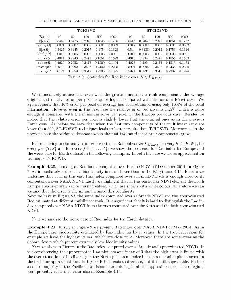
E[epO] 0.5442 0.3476 0.2949 0.1845 0.1735 0.5416 0.3467 0.2945 0.1851 0.1752

Var[epO] 0.0021 0.0007 0.0007 0.0004 0.0002 0.0018 0.0007 0.0007 0.0004 0.0002

E[epR] 0.5425 0.3445 0.2917 0.175 0.1628 0.54 0.3436 0.2913 0.1756 0.1646

Var[epR] 0.0019 0.0006 0.0006 0.0003 0.0001 0.0017 0.0005 0.0006 0.0003 0.0001

min epO 0.4614 0.2943 0.2472 0.1551 0.1523 0.4613 0.294 0.2475 0.1555 0.1539

min epR 0.4625 0.2952 0.2473 0.1509 0.1454 0.4623 0.295 0.2473 0.1513 0.1473

max epO 0.613 0.3992 0.3498 0.2442 0.2295 0.5991 0.3994 0.3497 0.2435 0.2306

max epR 0.6124 0.3859 0.3512 0.2396 0.1895 0.5971 0.3834 0.3511 0.2387 0.1926

Table 9. Statistics for Rao index over N ∈ NR,W,t,j .

We immediately notice that even with the greatest multilinear rank components, the averageoriginal and relative error per pixel is quite high if compared with the ones in Renyi case. Weagain remark that 16% error per pixel on average has been obtained using only 16.4% of the totalinformation. However even in the best case the relative error per pixel is 14.5%, which is quiteenough if compared with the minimum error per pixel in the Europe previous case. Besides wenotice that the relative error per pixel is slightly lower that the original ones as in the previousEarth case. As before we have that when the first two components of the multilinear rank arelower than 500, ST-HOSVD techniques leads to better results than T-HOSVD. Moreover as in theprevious case the variance decreases when the first two multilinear rank components grow.

Before moving to the analysis of error related to Rao index over NN,h,p,j for every h ∈ {E,W}, forevery p ∈ {T, S} and for every j ∈ {1, . . . , 5}, we show the best case for Rao index for Europe andthe worst case for Earth dataset in the following examples. In both the case we use as approximationtechnique T-HOSVD.

Example 4.20. Looking at Rao index computed over Europe NDVI of December 2014, in Figure7, we immediately notice that biodiversity is much lower than in the Renyi case, 4.14. Besides weunderline that even in this case Rao index computed over self-made NDVIs is enough close to itscomputation over NASA NDVI. Lastly we highlight that in this particular NDVI element the northEurope area is entirely set to missing values, which are shown with white colour. Therefore we canassume that the error is the minimum since this peculiarity.Next we have in Figure 8A the same index computed over self-made NDVI and the approximatedRao estimated at different multilinear rank. It is significant that it is hard to distinguish the Rao in-dex computed over NASA NDVI from the ones computed over the forth and the fifth approximatedNDVI.

Next we analyse the worst case of Rao index for the Earth dataset.

Example 4.21. Firstly in Figure 9 we present Rao index over NASA NDVI of May 2014. As inthe Europe case, biodiversity estimated by Rao index has lower values. In the tropical regions forexample we have the highest values, which are close to 2. Moreover there are some areas as theSahara desert which present extremely low biodiversity values.

Next we show in Figure 10 the Rao index computed over self-made and approximated NDVIs. Itis clear observing the approximated Rao pictures and index of 9 that the high error is linked withthe overestimation of biodiversity in the North pole area. Indeed it is a remarkable phenomenon inthe first four approximations. In Figure 10F it tends to decrease, but it is still appreciable. Besidesalso the majority of the Pacific ocean islands are missing in all the approximations. These regionswere probably related to error also in Example 4.15.


2

1

0

Figure 7. Rao index computed over NASA NDVI of December 2014.

As before, the following step is computing Rao index over approximated NDVI of NN,h,t,j forevery h ∈ {E,W}, for every t ∈ {T, S} and j ∈ {1, . . . , 5}.

Definition 4.22. Let RN,h,t,j be the set of Rao index computed over elements of NN,h,t,j for everyh ∈ {E,W}, for every t ∈ {T, S} and for every j ∈ {1, . . . , 5} and we call them ij-approximatedestimates for every ij ∈ R and for every j ∈ {1, . . . , 5}.

Then we compute the error with respect to the original estimates, i.e.∥∥∥Ak − Ck,j∥∥∥for every Ak ∈ Rh and for every Ck,j ∈ RN,h,T,j ∪ RN,h,S,j , for every k ∈ {1, . . . , nh}, for everyj ∈ {1, . . . , 5} and for every h ∈ {E,W}. Moreover we compute the error with respect to relativeestimates, i.e. ∥∥∥Bk − Ck,j∥∥∥for every Bk ∈ Rh and for every Ck,j ∈ RN,h,T,j ∪ RN,h,S,j , for every k ∈ {1, . . . , nh}, for everyj ∈ {1, . . . , 5} and for every h ∈ {E,W}.

In conclusion we report some statistics about the original and the relative errors per pixel, storedrespectively in vector epO and epR for the Europe dataset. Comparing Table 8 with Table 10, wenotice that the average original and relative error per pixel are greater in the second case. Inother words, starting from a tensor with repeated NIR band is not convenient for computing Raoindex over Europe elements. Besides we underline that the minimum relative and original error arerealised when the starting tensor has RED band repeated. We can not affirm nothing about themaximum original and relative error, since for ij ∈ {10, 100} it is lower when the repeated bandis the NIR, while for ij ∈ {50, 500, 1000} when it is repeated RED band. Lastly we highlight asalways for the Europe dataset that the average original error is lower than the relative one. As inthe repeated RED case, we remark that ST-HOSVD is convenient when the first two componentsof multilinear are strictly lower than 500, otherwise T-HOSVD provides better results. Then we


(A) Relativeapproximation





(F) Compo-nent rank 1000compression

Figure 8. Approximation of Rao index for December 2014, from NDVI of NR,E,S,j ∪ NE .

T-HOSVD ST-HOSVD

Rank 10 50 100 500 1000 10 50 100 500 1000

E[epO] 0.6392 0.3641 0.2962 0.2094 0.1969 0.6332 0.3632 0.2953 0.2111 0.1991

Var[epO] 0.0049 0.0012 0.001 0.003 0.0029 0.0044 0.0012 0.0009 0.0029 0.0029

E[epR] 0.6396 0.3647 0.2974 0.2115 0.1999 0.6335 0.3638 0.2964 0.2131 0.2021

Var[epR] 0.0048 0.0013 0.0011 0.0036 0.0043 0.0044 0.0013 0.0011 0.0035 0.0042

min epO 0.4801 0.2741 0.2204 0.1357 0.1246 0.4777 0.2739 0.2202 0.1378 0.1269

min epR 0.4801 0.2741 0.2204 0.1357 0.1246 0.4778 0.2739 0.2202 0.1377 0.1269

max epO 0.7505 0.4167 0.3497 0.3933 0.3953 0.7403 0.4155 0.3491 0.3946 0.3949

max epR 0.7504 0.4444 0.4259 0.4487 0.5458 0.7402 0.4506 0.4193 0.4472 0.547

Table 10. Statistics for Rao index over N ∈ NN,E,t,j .


2

1

0

Figure 9. Rao index computed over NASA NDVI of December 2014.

(A) Relative approximation (B) Component rank 10compression



(E) Component rank 500compression

(F) Component rank 1000compression

Figure 10. Approximation of Rao index for May 2014, from NDVI of NR,W,S,j ∪ NW .


present the final statistics for original and relative errors of Rao estimates for Earth dataset. Asalways in vector epO and in epR are respectively stored the original and relative errors per pixel.

T-HOSVD ST-HOSVD

Rank 10 50 100 500 1000 10 50 100 500 1000

E[epO] 0.5366 0.3419 0.2869 0.1754 0.1636 0.5353 0.3417 0.287 0.1761 0.1651

Var[epO] 0.0023 0.0008 0.0007 0.0005 0.0003 0.0022 0.0008 0.0007 0.0005 0.0003

E[epR] 0.535 0.3389 0.2835 0.1657 0.1525 0.5337 0.3387 0.2836 0.1664 0.1541

Var[epR] 0.0021 0.0006 0.0006 0.0003 0.0001 0.002 0.0006 0.0006 0.0003 0.0001

min epO 0.4481 0.2873 0.2385 0.1431 0.1357 0.4487 0.2881 0.2394 0.1437 0.1376

min epR 0.4486 0.2885 0.2385 0.1382 0.1331 0.4483 0.2887 0.2394 0.1391 0.135

max epO 0.6063 0.3887 0.3458 0.2352 0.226 0.6006 0.389 0.3466 0.2352 0.2267

max epR 0.6057 0.375 0.3478 0.2307 0.1746 0.5997 0.3743 0.3487 0.2314 0.1768

Table 11. Statistics for Rao index over N ∈ NN,W,t,j .

In this case comparing Table 9 with Table 11, we notice that starting tensors with repeated NIRband provides on average better results. Indeed for both the decomposition techniques at the fifthapproximation the average original and relative error per pixel is around 17.5% in the first caseand 16.5% in the second one. This 1% difference between the RED and NIR case is present alsoin the minimum and maximum relative and original error per pixel for both the decompositiontechniques. Besides we underline that also in this case ST-HOSVD is convenient when the firsttwo multilinear components are lower than 100, otherwise T-HOSVD is preferable. In conclusionto these analysis we want to empathise that an average error of 16.5% per pixel is not much, if weremind that we use only 16.4% of the total information available.Lastly as before, we display the Rao index computed for December 2014 and May 2014, startingfrom tensors with repeated NIR bands.

Example 4.23. Firstly we remark that December 2014 realises the minimum original and relativeerror, also starting from tensors with repeated NIR band. In Figure 11 there are approximatedRao estimates at different multilinear rank, for this NIR repeated case. As before, our eyes hardlyperceive differences between Rao computed over NASA or self-made NDVI and over the last threeapproximated NDVIs.

Example 4.24. Firstly we remark that May 2014 do not realise the minimum original and relativeerror starting from tensors with repeated NIR band. Therefore these are not the worst approxima-tions in the Earth dataset, in this second case. In Figure 12 there are approximated Rao estimatesat different multilinear rank, for this NIR repeated case. As in Figure 10 the problematic areas arethe North pole and the Pacific ocean. Indeed we notice that there is a biodiversity overestimationin the Arctic regions, which decreases for increasing multilinear rank components. Moreover evenin the fifth approximation there are missing island in the Pacific ocean. However we can not easilynotice much difference with respect to Figure 10.

5. Conclusion

We have shown that the presented approach is extremely convenient for Renyi index estimationto save storage memory. As reported in Tables 4,6, 5 and 7 the average error per pixel is around5.5% for Earth dataset and is close to 7.6% for the Europe’s one when using respectively 16.4%and 14.8% of the total tensor information. Moreover we have seen that starting from tensor withrepeated NIR bands is more convenient than with RED repeated, in the Renyi case. For Rao casestarting with twice NIR rasters is more convenient only for Earth dataset. Lastly we have remarked


(A) Compo-nent rank 10compression




%(E) Compo-nent rank 1000compression

2

1

0

Figure 11. Approximation of Rao index for December 2014, from NDVI of NN,E,S,j .

that in Renyi case T-HOSVD makes on biodiversity estimation lower error than ST-HOSVD whenthe first two multilinear rank components are relatively low.

In the Rao case we face greater on average original and relative error per pixel. Indeed in Tables8 and 9 we have an average error per pixel close to 19.5% and 17% for Europe and for Earth datasetrespectively. In this case we have noticed that the roles of T-HOSVD and ST-HOSVD are inverted.Indeed T-HOSVD makes on biodiversity estimation lower error than ST-HOSVD with the first twomultilinear rank components are relatively great.

In conclusion we believe that the presented work might help ecologists in their remote sensedplant biodiversity estimation. Indeed fixed a certain accuracy, they can compress through T-HOSVD and ST-HOSVD the tensors with NIR and RED bands, to save storage memory and atthe same time computing with fixed tolerance the biodiversity estimates.Lastly if it was possible to directly download decomposed tensors, ecologists would benefit of asignificant computer memory saving.


(A) Component rank 10compression

(B) Component rank 50compression



(E) Component rank 1000 compression

2

1

0

Figure 12. Approximation of Rao index for May 2014, from NDVI of NN,W,S,j .

References

[ADKM11] E. Acar, D.M. Dunlavy, T.G. Kolda, and M. Mørup, Scalable tensor factorizations for incomplete data,Chemometrics and Intelligent Laboratory Systems 106 (2011), no. 1, 41 – 56, Multiway and MultisetData Analysis.

[BBC+19] E. Ballico, A. Bernardi, I. Carusotto, S. Mazzucchi, and V. Moretti, Introduction, Lecture Notes of theUnione Matematica Italiana (2019), 1–4.

[BBCM11] A. Bernardi, J. Brachat, P. Comon, and B. Mourrain, Multihomogeneous polynomial decompositionusing moment matrices, ISSAC 2011—Proceedings of the 36th International Symposium on Symbolicand Algebraic Computation, ACM, New York, 2011, pp. 35–42. MR 2895192

[BBK+16] M. Benzi, D. Bini, D. Kressner, H. Munthe-Kaas, and C. Van Loan, Exploiting hidden structure inmatrix computations: Algorithms and applications, Lecture Notes in Mathematics (2016).

[BDHM17] A. Bernardi, N.S. Daleo, J.D. Hauenstein, and B. Mourrain, Tensor decomposition and homotopy con-tinuation, Differential Geometry and its Applications 55 (2017), 78 – 105, Geometry and complexitytheory.


[BDHR17] A. Boralevi, J. Draisma, E. Horobet, and E. Robeva, Orthogonal and unitary tensor decomposition froman algebraic perspective, Israel J. Math. 222 (2017), no. 1, 223–260. MR 3736505

[Bje51] A. Bjerhammar, Application of calculus of matrices to method of least squares; with special referencesto geodetic calculations, Trans. Roy. Inst. Tech. Stockholm (1951).

[BP94] D. Bini and V.Y. Pan, Fundamental computations with general and dense structured matrices, Polyno-mial and Matrix Computations (1994), 81–227.

[Chi07] A. Chiarucci, To sample or not to sample? That is the question ... for the vegetation scientist, FoliaGeobotanica 42 (2007), no. 2, 209.

[CJ] E. Chuvieco and C. Justice, Nasa earth observation satellite missions for global change research, EarthObservation of Global Change, 23–47.

[CW11] J.B. Campbell and R.H. Wynne, Introduction to remote sensing, 5 ed., vol. 1, Guilford Publications,2011.

[Did18a] K. Didan, Mod13c2 modis/terra vegetation indices monthly l3 global 0.05deg cmg v006. 2015,https://doi.org/10.5067/MODIS/MOD13C2.006, 2010–2018.

[Did18b] , MOD13A3 MODIS/Terra vegetation Indices Monthly L3 Global 1km SIN Grid V006. 2015,https://doi.org/10.5067/MODIS/MOD13A3.006, 2011–2018.

[DLDMV00] L. De Lathauwer, B. De Moor, and J. Vandewalle, A multilinear singular value decomposition, SIAMJournal on Matrix Analysis and Applications 21 (2000), no. 4, 1253–1278.

[DOT18] J. Draisma, G. Ottaviani, and A. Tocino, Best rank-k approximations for tensors: generalizing eckart-young, Research in the Mathematical Sciences 5 (2018), 27.

[dSL08] V. de Silva and L.-H. Lim, Tensor rank and the ill-posedness of the best low-rank approximation problem,SIAM J. Matrix Anal. Appl. 30 (2008), 1084–1127.

[EY36] C. Eckart and G. Young, The approximation of one matrix by another of lower rank, Psychometrika 1(1936), 211–218.

[GSR+14] M. Gerster, P. Silvi, M. Rizzi, R. Fazio, T. Calarco, and S. Montangero, Unconstrained tree tensornetwork: An adaptive gauge picture for enhanced performance, Physical Review B 90 (2014), no. 12,125154.

[GVL96] G.H. Golub and C.F. Van Loan, Matrix computations, third ed., The Johns Hopkins University Press,1996.

[Ian19] M. Iannacito, Biodiversity index computation, https://zenodo.org/badge/latestdoi/196228972,https://github.com/MartinaIannacito/Biodiversity-index-computation, July 2019.

[IAVHDL11] M. Ishteva, P.-A. Absil, S. Van Huffel, and L. De Lathauwer, Best low multilinear rank approximation ofhigher-order tensors, based on the riemannian trust-region scheme, Society for Industrial and AppliedMathematics 32 (2011), no. 1, 115–135.

[JOP ] E. Jones, T. Oliphant, and P. Peterson, Scipy: Open source scientific tools for python,http://www.scipy.org/, 2001–.

[JXP12] Y.-J. Jia, P.-F. Xu, and X.-M. Pei, An investigation of image compression using block singular valuedecomposition, Communications and Information Processing (2012), 723–731.

[KPAP19] J. Kossaifi, Y. Panagakis, A. Anandkumar, and M. Pantic, Tensorly: Tensor learning in python, Journalof Machine Learning Research 20 (2019), no. 26, 1–6.

[LC10] L.-H. Lim and P. Comon, Multiarray signal processing: Tensor decomposition meets compressed sensing,Comptes Rendus Mecanique 338 (2010), no. 6, 311 – 320.

[Mir59] L. Mirsky, On the trace of matrix products, Mathematische Nachrichten 20 (1959), 171–174.[Mir60] , Symmetric gauge functions and unitarily invariant norms, Q. J. Math. Oxf. II. Ser. 11 (1960),

50–59.[Moo20] E.H. Moore, On the reciprocal of the general algebraic matrix, Bulletin of the American Mathematical

Society 26 (1920), 394–95.[Oli06] T.E. Oliphant, A guide to numpy, vol. 1, Trelgol Publishing USA, 2006.[Pen55] R. Penrose, A generalized inverse for matrices, Proceedings of the Cambridge Philosophical Society 51

(1955), 406–13.[RBC+10] D. Rocchini, N. Balkenhol, G. A. Carter, G. M. Foody, T.W. Gillespie, K.S. He, S. Kark, N. Levin,

K. Lucas, M. Luoto, H. Nagendra, J. Oldeland, C. Ricotta, J. Southworth, and M. Neteler, Remotelysensed spectral heterogeneity as a proxy of species diversity: Recent advances and open challenges,Ecological Informatics 5 (2010), no. 5, 318–329.

[RDB+13] D. Rocchini, L. Delucchi, G. Bacaro, P. Cavallini, H. Feilhauer, G.M. Foody, K.S. He, H. Nagendra,C. Porta, C. Ricotta, S. Schmidtlein, L.D. Spano, M. Wegmann, and M. Neteler, Calculating landscapediversity with information-theory based indices: A GRASS GIS solution, Ecological Informatics 17(2013), 82–93.


[RHSD74] J. W. Rouse, Jr., R. H. Haas, J. A. Schell, and D. W. Deering, Monitoring vegetation systems in thegreat plains with erts, NASA Special Publication 351 (1974), 309.

[RMR17] D. Rocchini, M. Marcantonio, and C. Ricotta, Measuring rao’s q diversity index from remote sensing:An open source solution, Ecological Indicators 72 (2017), 234–238.

[Sch07] E. Schmidt, Zur theorie der linearen und nichtlinearen integralgleichungen, Mathematische Annalen 65(1907), 433–476.

[SSV+05] C. Schon, E. Solano, F. Verstraete, J.I. Cirac, and M.M. Wolf, Sequential generation of entangledmultiqubit states, Phys. Rev. Lett. 95 (2005), 110503.

[Ste93] G.W. Stewart, On the early history of the singular value decomposition, SIAM Review 35 (1993), 551–566.

[STG+19] P. Silvi, F. Tschirsich, M. Gerster, J. Junemann, D. Jaschke, M. Rizzi, and S. Montangero, The TensorNetworks Anthology: Simulation techniques for many-body quantum lattice systems, SciPost Phys. Lect.Notes (2019), 8.

[Var ] G. Varoquaux, Joblib: running python functions as pipeline jobs, https://github.com/joblib/joblib,2009–.

[VNVM14] N. Vannieuwenhoven, J. Nicaise, R. Vandebril, and K. Meerbergen, On generic nonexistence of theschmidt–eckart–young decomposition for complex tensors, SIAM Journal on Matrix Analysis and Ap-plications 35 (2014), 886–903.

[VVM12] N. Vannieuwenhoven, R. Vandebril, and K. Meerbergen, A new truncation strategy for the higher-ordersingular value decomposition, SIAM Journal on Scientific Computing 34 (2012), 1027–1052.

[WBWJ15] L. Wang, J. Bai, J. Wu, and G. Jeon, Hyperspectral image compression based on lapped transform andtucker decomposition, Signal Processing: Image Communication 36 (2015), 63 – 69.

[ZFL+19] F. Zellweger, P.D. Frenne, J. Lenoir, D. Rocchini, and D. Coomes, Advances in Microclimate EcologyArising from Remote Sensing, Trends in Ecology & Evolution 34 (2019), no. 4, 327–341.

6. Appendix

6.1. Rao’s and Renyi’s codes. Remind that for every raster of size (m,n), fixed l the side of themoving window, the biodiversity index is computed l ×m× n times. To speed up the entire workwe decide to implement a parallel version of the biodiversity index algorithm. When a computerexecutes a parallel functions its cores perform independently different tasks at the same time. In ourcase we want that each core of the used machine works on different position of the moving window.Consequently to implement this mechanism we needed a parallel computing library compatiblewith Python, the chosen programming language. We preferred Joblib, cf. [Var ], since its ease ofuse. Other two used libraries are itertools, to create iterable elements and spatial from SciPy,to compute the distance element wise for two matrices. The main Rao computation code is

#### computation

import numpy as np

import scipy

from scipy import spatial

import itertools

#### parallelisation

import joblib

from joblib import Parallel, delayed

import multiprocessing

def raop(rw):

def raout (cl, rw = rw, rasterm = rasterm, missing = missing, w = w, distance_m

↪→ = distance_m):

tw_labels, tw_values = np.unique(rasterm[(rw-w):(rw+w+1),(cl-w):(cl+w+1)],

↪→ return_counts=True)

if len(np.where(tw_labels == missing)) != 0:

tw_values = np.delete( tw_values, np.where(tw_labels == missing))


tw_labels = np.delete( tw_labels, np.where(tw_labels == missing))

if len(tw_values) > 1:

d1 = spatial.distance.cdist(np.diag(tw_labels), np.diag(tw_labels),

↪→ distance_m)

p = tw_values/np.sum(tw_values)

p1 = np.zeros((len(tw_values),len(tw_values)))

comb = np.array([x[0]*x[1] for x in list(itertools.combinations(p, 2))])

p1[np.triu_indices(len(tw_values), k=1)] = comb

p1[np.tril_indices(len(tw_values), k=-1)] = comb

return ((np.sum(np.multiply(p1,d1))))

elif len(tw_values) == 1:

return (((0)))

else:

return ((missing))

Raout = Parallel(n_jobs = NcCores)(delayed(raout)(cl) for cl in range(w,c-w))

return (Raout)

out[w:(r-w), w:(c-w)] = (np.asarray(Parallel(n_jobs = NcCores)(delayed(raop)(rw)

↪→ for rw in range(w,(r-w)))).reshape(r-2*w,c-2*w))

Since the moving window scrolls over rows and over columns, we define two parallelised functions oneinside the others, raop whose variable is just the row index and raout. This second function takesas variable the column index and has other set parameters: rasterm the raster, rw the row index,missing a value used in the raster when data are not present, w the window side and a functiondistance_m to compute the distance between raster values. The first step is storing the valuesand their frequencies of the raster area covered by the moving window in the arrays tw_labels

and tw_values respectively. Then we check if there is the missing value in the considered area:if it is present, we remove it and its frequency from the storing arrays. Next if there are atleast two different elements in the tw_values array, we compute their distance with the functionspatial.distance.cdist and save the result in the d1 matrix. In p we put the relative frequencies,obtained from the absolute ones. We define a 0 matrix p1, with the same size of d1. We computeand store in comb all the possible combination between different elements of vector p. We assignthese values to the upper and lower triangular part of the matrix p1. Lastly we return the sumof the elements of the product matrix between d1 and p1. Notice that the product matrix willcoherently have diagonal null elements, since the distance between a pixel value and itself is 0.If there is just one element in vector tw_values, we return 0 since the difference between a pixelvalue and itself is 0. Otherwise, if tw_values is an empty vector, we return missing. Insidefunction raop we define function raout and we do the first Parallel call. Outside it we do thesecond Parallel call. Notice that this function is thought to compute Rao’s index when themoving window is completely contained into the raster. When this condition is not satisfied, tospeed up computation, there is a special implementation of Rao’s, available here [Ian19]. With asimilar approach, we implemented Renyi’s index, whose core is

#### computation

import numpy as np

import scipy

#### parallelisation

import joblib

from joblib import Parallel, delayed

import multiprocessing


def IndexOP (rw):

def IndexOut (cl, rw = rw, rasterm = rasterm, missing = missing, w = w, alpha=

↪→ alpha, base = base):

tw_labels, tw_values = np.unique(rasterm[(rw-w):(rw+w+1),(cl-w):(cl+w+1)],

↪→ return_counts=True)

if len(np.where(tw_labels == missing)[0]) != 0:

tw_values = np.delete( tw_values, np.where(tw_labels == missing))

if len(tw_values) != 0:

p = tw_values/np.sum(tw_values)

if np.log(np.sum(p**alpha)) == 0:

return(0)

else:

return((1/(1-alpha)) * np.log(np.sum(p**alpha)) / np.log(base))

else:

return (missing)

Index_Out = Parallel(n_jobs = NcCores)(delayed(IndexOut)(cl) for cl in range(w,

↪→ c-w))

return (Index_Out)

out[w:(r-w), w:(c-w)] = np.asarray(Parallel(n_jobs = NcCores)(delayed(IndexOP)(rw

↪→ ) for rw in range(w,r-w))).reshape(r-2*w,c-2*w)

Similarly we declare function IndexOP, with just row index as variable and inside it functionIndexOut. This one takes as parameters some equals to raout’s ones. The variable proper ofIndexOut are alpha, the Renyi’s parameter, and base, the logarithm base. The code structureis similar to raout. We compute and store the values, present inside the raster area covered bythe moving window, and their frequencies. We check and in case delete missing value and itsfrequency. If there is still an element into tw_values, we compute the relative frequencies andreturn the Renyi index. We test if the index final value is 0 and return 0 to avoid sign problem. Iftw_values is an empty vector, we return missing value. We do a first Parallel call of IndexOutinside IndexOP and a second one of IndexOP outside it. Even in this case the presented code willwork only when the moving window is entirely contained in the raster. To speed up the computa-tions, we develop a special version of this code which works when the moving window is not fullycontained. It is available here [Ian19].

6.2. Approximation codes for T-HOSVD. In order to implement the approximation Algo-rithm 1 of T-HOSVD we need a python library expressly developed to manage tensors. Moreoverwe also want that this library to interact properly with NumPy the python most used library fornumerical computation, cf. [Oli06]. Therefore we choose TensorLy, cf. [KPAP19]. This recentlydeveloped library, firstly presented in 2016, wants to make tensor study and manipulation easyand accessible. Besides their creators projected TensorLy to perfectly match with other famouspython libraries, as NumPy, SciPy. They developed most of the main tensor operations and relatedfunctions. To compute the singular value decomposition of tensors flattening, the central step inT-HOSVD and ST-HOSVD algorithm, we need a python function able to manage huge arrays. Thisis not a trivial task, since development of python functions is left to singular initiative. We decideto use svds function from SciPy sparse linear algebra function, cf. [JOP ]. This implementation ofSVD takes advantage of matrix sparsity in performing the matrix-vector multiplication. The finalimplementation of T-HOSVD is

import numpy as np


import tensorly as tl

from tensorly import decomposition as decompose

from tensorly import tenalg as Tla

import scipy


from scipy.sparse.linalg import svds

def T_hosvd(T, rango, projector = Ture):

L = []

dim = T.shape

for i in range(len(dim)):

flat = tl.unfold(T,i)

res = svds(flat, k = rango[i])

L.append(np.transpose(res[0][0:dim[i], :]))

core = Tla.multi_mode_dot(T,L)

if projector:

P = [np.transpose(u) for u in L]

return [core,P]

return core

This function takes as input variable a tensor T and a list or a tuple, whose values are the targetmultilinear rank components. Inside the T_hosvd we declare an empty list, L, in which at the i-thstep we store matrix U_i from the thin SVD of the i-th flattening for every i ∈ {1, . . . , d}. The dim

variable is a tuple containing the size of tensor T. Then for each direction we compute the flatteningand its SVD. After the for loop, we get the core tensor with the multilinear product between a listof matrices, our projectors, and the original tensor T. Notice that there is the option projector,with True as default value, to return a list L containing the projectors matrices together with thestandard result, i.e. the core tensor.

6.3. Approximation codes for ST-HOSVD. The ST-HOSVD implementation of Algorithm 2is

import numpy as np

import tensorly as tl

from tensorly import decomposition as decompose

from tensorly import tenalg as Tla

import scipy


from scipy.sparse.linalg import svds

def ST_hosvd(T, rango, projector = True):

dim = T.shape

core = T

if projector:

P=[]

for i in range(len(dim)):

flat = tl.unfold(core,i)

res = svds(flat, k=rango[i])

core = Tla.mode_dot(core,np.transpose(res[0][0:dim[i],:]),mode=i)


if projector:

P.append(res[0][0:dim[i],:])

if projector:

return [core,P]

return core

The input arguments of ST-HOSVD and T-HOSVD implementations are the same. The firstdifference with T_hosvd is the initial declaration of core tensor, set equal to T. Next we highlightthat only if the projector variable is True, we initialize an empty list to store the projectorsmatrices. Another difference is the computation of the core tensor inside the for loop with thecomponent wise product between matrix and tensor, fixed a certain direction. The basic output isstill the final core tensor.

high order singular value decomposition for plant

Documents