parallel algorithms for the singular value decomposition · parallel algorithms for the singular...
TRANSCRIPT
�
�
Erricos John: Handbook on Parallel Computing and Statistics DK2384 c004 2005/7/20 20:27�
�
�
�
�
�
4Parallel Algorithms forthe Singular ValueDecomposition
Michael W. Berry, Dani Mezher, Bernard Philippe,and Ahmed Sameh
CONTENTS
Abstract . . . . . . . . . . . . . . . . . . . . . . . . . . . . . . . . . . . . . . . . . . . . . . . . . . . . . . . . . . . . . . . . . . . . . . . . . . . . . . . . . 1184.1 Introduction. . . . . . . . . . . . . . . . . . . . . . . . . . . . . . . . . . . . . . . . . . . . . . . . . . . . . . . . . . . . . . . . . . . . . . . . 118
4.1.1 Basics . . . . . . . . . . . . . . . . . . . . . . . . . . . . . . . . . . . . . . . . . . . . . . . . . . . . . . . . . . . . . . . . . . . . . . 1184.1.2 Sensitivity of the Smallest Singular Value . . . . . . . . . . . . . . . . . . . . . . . . . . . . . . . . . . . . 1204.1.3 Distance to Singularity — Pseudospectrum . . . . . . . . . . . . . . . . . . . . . . . . . . . . . . . . . . . 122
4.2 Jacobi Methods for Dense Matrices . . . . . . . . . . . . . . . . . . . . . . . . . . . . . . . . . . . . . . . . . . . . . . . . . 1234.2.1 Two-sided Jacobi Scheme [2JAC] . . . . . . . . . . . . . . . . . . . . . . . . . . . . . . . . . . . . . . . . . . . . 1234.2.2 One-Sided Jacobi Scheme [1JAC] . . . . . . . . . . . . . . . . . . . . . . . . . . . . . . . . . . . . . . . . . . . 1274.2.3 Algorithm [QJAC] . . . . . . . . . . . . . . . . . . . . . . . . . . . . . . . . . . . . . . . . . . . . . . . . . . . . . . . . . . 1304.2.4 Block-Jacobi Algorithms . . . . . . . . . . . . . . . . . . . . . . . . . . . . . . . . . . . . . . . . . . . . . . . . . . . . 132
4.3 Methods for large and sparse matrices . . . . . . . . . . . . . . . . . . . . . . . . . . . . . . . . . . . . . . . . . . . . . . . 1334.3.1 Sparse Storages and Linear Systems . . . . . . . . . . . . . . . . . . . . . . . . . . . . . . . . . . . . . . . . . . 1334.3.2 Subspace Iteration [SISVD] . . . . . . . . . . . . . . . . . . . . . . . . . . . . . . . . . . . . . . . . . . . . . . . . . 1344.3.3 Lanczos Methods . . . . . . . . . . . . . . . . . . . . . . . . . . . . . . . . . . . . . . . . . . . . . . . . . . . . . . . . . . . 136
4.3.3.1 The Single-Vector Lanczos Method [LASVD] . . . . . . . . . . . . . . . . . . . . . . . . 1364.3.3.2 The Block Lanczos Method [BLSVD] . . . . . . . . . . . . . . . . . . . . . . . . . . . . . . . . 138
4.3.4 The Trace Minimization Method [TRSVD] . . . . . . . . . . . . . . . . . . . . . . . . . . . . . . . . . . . . 1404.3.4.1 Polynomial Acceleration Techniques for [TRSVD] . . . . . . . . . . . . . . . . . . . 1424.3.4.2 Shifting Strategy for [TRSVD] . . . . . . . . . . . . . . . . . . . . . . . . . . . . . . . . . . . . . . . 143
4.3.5 Refinement of Left Singular Vectors . . . . . . . . . . . . . . . . . . . . . . . . . . . . . . . . . . . . . . . . . . 1444.3.6 The Davidson Methods . . . . . . . . . . . . . . . . . . . . . . . . . . . . . . . . . . . . . . . . . . . . . . . . . . . . . . 147
4.3.6.1 General Framework of the Methods . . . . . . . . . . . . . . . . . . . . . . . . . . . . . . . . . 1474.3.6.2 How do the Davidson Methods Differ? . . . . . . . . . . . . . . . . . . . . . . . . . . . . . . 1494.3.6.3 Application to the Computation of the Smallest Singular Value . . . . . . . 151
4.4 Parallel computation for Sparse Matrices . . . . . . . . . . . . . . . . . . . . . . . . . . . . . . . . . . . . . . . . . . . . 1524.4.1 Parallel Sparse Matrix-Vector Multiplications . . . . . . . . . . . . . . . . . . . . . . . . . . . . . . . . . 1524.4.2 A Parallel Scheme for Basis Orthogonalization . . . . . . . . . . . . . . . . . . . . . . . . . . . . . . . 1544.4.3 Computing the Smallest Singular Value on Several Processors . . . . . . . . . . . . . . . . . 156
4.5 Application: parallel computation of a pseudospectrum . . . . . . . . . . . . . . . . . . . . . . . . . . . . . . 1574.5.1 Parallel Path-Following Algorithm using Triangles . . . . . . . . . . . . . . . . . . . . . . . . . . . . 1574.5.2 Speedup and Efficiency . . . . . . . . . . . . . . . . . . . . . . . . . . . . . . . . . . . . . . . . . . . . . . . . . . . . . . 1584.5.3 Test Problems . . . . . . . . . . . . . . . . . . . . . . . . . . . . . . . . . . . . . . . . . . . . . . . . . . . . . . . . . . . . . . . 159
References . . . . . . . . . . . . . . . . . . . . . . . . . . . . . . . . . . . . . . . . . . . . . . . . . . . . . . . . . . . . . . . . . . . . . . . . . . . . . . 160
117
�
�
Erricos John: Handbook on Parallel Computing and Statistics DK2384 c004 2005/7/20 20:27�
�
�
�
�
�
118 Handbook on Parallel Computing and Statistics
ABSTRACT
The goal of the survey is to review the state-of-the-art of computing the Singular Value Decompo-sition (SVD) of dense and sparse matrices, with some emphasis on those schemes that are suitablefor parallel computing platforms. For dense matrices, we present those schemes that yield the com-plete decomposition, whereas for sparse matrices we describe schemes that yield only the extremalsingular triplets. Special attention is devoted to the computation of the smallest singular valueswhich are normally the most difficult to evaluate but which provide a measure of the distance tosingularity of the matrix under consideration. Also, we conclude with the presentation of a parallelmethod for computing pseudospectra, which depends on computing the smallest singular values.
4.1 INTRODUCTION
4.1.1 BASICS
The Singular Value Decomposition (SVD) is a powerful computational tool. Modern algorithmsfor obtaining such a decomposition of general matrices have had a profound impact on numerousapplications in science and engineering disciplines. The SVD is commonly used in the solutionof unconstrained linear least squares problems, matrix rank estimation, and canonical correlationanalysis. In computational science, it is commonly applied in domains such as information retrieval,seismic reflection tomography, and real-time signal processing [1].
In what follows, we will provide a brief survey of some parallel algorithms for obtaining theSVD for dense, and large sparse matrices. For sparse matrices, however, we focus mainly on theproblem of obtaining the smallest singular triplets.
To introduce the notations of the chapter, the basic facts related to SVD are presented withoutproof. Complete presentations are given in many text books, as for instance [2, 3].
Theorem 4.1 [SVD]If A ∈ R
m×n is a real matrix, then there exist orthogonal matrices
U = [u1, . . . , um] ∈ Rm×m and V = [v1, . . . , vn] ∈ R
n×n
such that
� = U T AV = diag(σ1, . . . , σp) ∈ Rm×n, p = min(m, n) (4.1)
where σ1 ≥ σ2 ≥ · · · ≥ σp ≥ 0.
Definition 4.1 The singular values of A are the real numbers σ1 ≥ σ2 ≥ · · · ≥ σp ≥ 0. They areuniquely defined. For every singular value σi (i = 1, . . . , p), the vectors ui and vi are respectivelythe left and right singular vectors of A associated with σi .
More generally, the theorem holds in the complex field but with the inner products and orthog-onal matrices replaced by the Hermitian products and unitary matrices, respectively. The singularvalues, however, remain real nonnegative values.
Theorem 4.2 Let A ∈ Rm×n (m ≥ n) have the singular value decomposition
U T AV = �.
Then, the symmetric matrix
B = AT A ∈ Rn×n, (4.2)
�
�
Erricos John: Handbook on Parallel Computing and Statistics DK2384 c004 2005/7/20 20:27�
�
�
�
�
�
Parallel Algorithms for the Singular Value Decomposition 119
has eigenvalues σ12 ≥ · · · ≥ σn
2 ≥ 0, corresponding to the eigenvectors (vi ), (i = 1, · · · , n).The symmetric matrix
Aaug =(
0 AAT 0
)(4.3)
has eigenvalues ±σ1, . . . ,±σn, corresponding to the eigenvectors
1√2
(ui
±vi
), i = 1, . . . , n.
The matrix Aaug is called the augmented matrix.
Every method for computing singular values is based on one of these two matrices.The numerical accuracy of the i th approximate singular triplet (ui , σi , vi ) determined via the
eigensystem of the 2-cyclic matrix Aaug is then measured by the norm of the eigenpair residualvector ri defined by
‖ ri ‖2= [‖ Aaug(ui , vi )T − σi (ui , vi )
T ‖2]/[‖ ui ‖22 + ‖ vi ‖2
2]1/2,
which can also be written as
‖ ri ‖2= [(‖ Avi − σi ui ‖22 + ‖ ATui − σi vi ‖2
2)1/2]/ ‖ ui ‖2
2 + ‖ vi ‖22]1/2. (4.4)
The backward error [4]
ηi = max{‖ Avi − σi ui ‖2, ‖ ATui − σi vi ‖22}
may also be used as a measure of absolute accuracy. A normalizing factor can be introduced forassessing relative errors.
Alternatively, we may compute the SVD of A indirectly by the eigenpairs of either the n × nmatrix AT A or the m × m matrix AAT. If V = {v1, v2, . . . , vn} is the n × n orthogonal matrixrepresenting the eigenvectors of AT A, then
V T(AT A)V = diag(σ 21 , σ 2
2 , . . . , σ 2r , 0, . . . , 0︸ ︷︷ ︸
n−r
),
where σi is the i th nonzero singular value of A corresponding to the right singular vector vi . Thecorresponding left singular vector, ui , is then obtained as ui = (1/σi )Avi . Similarly, if U ={u1, u2, . . . , um} is the m × m orthogonal matrix representing the eigenvectors of AAT, then
U T(AAT)U = diag(σ 21 , σ 2
2 , . . . , σ 2r , 0, . . . 0︸ ︷︷ ︸
m−r
),
where σi is the i th nonzero singular value of A corresponding to the left singular vector ui . Thecorresponding right singular vector, vi , is then obtained as vi = (1/σi )ATui .
Computing the SVD of A via the eigensystems of either AT A or AAT may be adequate fordetermining the largest singular triplets of A, but some loss of accuracy may be observed for thesmallest singular triplets (see Ref. [5]). In fact, extremely small singular values of A (i.e., smallerthan
√ε‖A‖, where ε is the machine precision parameter) may be computed as zero eigenvalues
of AT A (or AAT). Whereas the smallest and largest singular values of A are the lower and upperbounds of the spectrum of AT A or AAT, the smallest singular values of A lie at the center of the
�
�
Erricos John: Handbook on Parallel Computing and Statistics DK2384 c004 2005/7/20 20:27�
�
�
�
�
�
120 Handbook on Parallel Computing and Statistics
spectrum of Aaug in (4.3). For computed eigenpairs of AT A and AAT, the norms of the i th eigenpairresiduals (corresponding to (4.4)) are given by
‖ ri ‖2=‖ AT Avi − σ 2i vi ‖2 / ‖ vi ‖2 and ‖ ri ‖2=‖ AATui − σ 2
i ui ‖2 / ‖ ui ‖2,
respectively. Thus, extremely high precision in computed eigenpairs may be necessary to computethe smallest singular triplets of A. This fact is analyzed in Section 4.1.2. Difficulties in approxi-mating the smallest singular values by any of the three equivalent symmetric eigenvalue problemswill be discussed in Section 4.4.
When A is a square nonsingular matrix, it may be advantageous in certain cases to com-pute the singular values of A−1 which are (1/σn) ≥ · · · ≥ (1/σ1). This approach has thedrawback of solving linear systems involving the matrix A, but when manageable, it provides amore robust algorithm. Such an alternative is of interest for some subspace methods (see Section4.3). Actually, the method can be extended to rectangular matrices of full rank by considering aQR-factorization:
Proposition 4.1 Let A ∈ Rm×n (m ≥ n) be of rank n. Let
A = Q R, where Q ∈ Rm×n and R ∈ R
n×n,
such that QT Q = In and R is upper triangular.The singular values of R are the same as the singular values of A.
Therefore, the smallest singular value of A can be computed from the largest eigenvalue of
(R−1 R−T) or of
(0 R−1
R−T 0
).
4.1.2 SENSITIVITY OF THE SMALLEST SINGULAR VALUE
To compute the smallest singular value in a reliable way, one must investigate the sensitivity of thesingular values with respect to perturbations of the matrix at hand.
Theorem 4.3 Let A ∈ Rn×n and ∆ ∈ R
n×n. The singular values of A and A + ∆ are respectivelydenoted
σ1 ≥ σ2 ≥ · · · ≥ σn
σ1 ≥ σ2 ≥ · · · ≥ σn .
They satisfy the following bounds
|σi − σi | ≤ ‖∆‖2, for i = 1, . . . , n.
Proof. See Ref. [3].
When applied to the smallest singular value, this result ends up with the following estimation.
Proposition 4.2 The relative condition number of the smallest singular value of a nonsingularmatrix A is equal to χ2(A) = ‖A‖2‖A−1‖2.
Proof. The result is obtained from
|σn − σn|σn
≤(‖∆‖2
‖A‖2
) ‖A‖2
σn.
�
�
Erricos John: Handbook on Parallel Computing and Statistics DK2384 c004 2005/7/20 20:27�
�
�
�
�
�
Parallel Algorithms for the Singular Value Decomposition 121
This means that the smallest singular value of an ill-conditioned matrix cannot be computed withhigh accuracy even with an algorithm of perfect arithmetic behavior (i.e., backward stable).
Recently, some progress has been made [6]. It is shown that for some special class of matrices,an accurate computation of the smallest singular value may be obtained via a combination of someQR-factorization with column pivoting and a one-sided Jacobi algorithm (see Section 4.2.2).
Because the nonzero singular values are roots of a polynomial (e.g., roots of the characteristicpolynomial of the augmented matrix), then when simple, they are differentiable with respect to theentries of the matrix. More precisely, one can states that:
Theorem 4.4 Let σ be a nonzero simple singular value of the matrix A = (ai j ) with u = (ui ) andv = (vi ) being the corresponding normalized left and right singular vectors. Then, the singularvalue is differentiable with respect to the matrix A, or
∂σ
∂ai j= uiv j , ∀i, j = 1, . . . , n.
Proof. See Ref. [7].
The effect of a perturbation of the matrix on the singular vectors can be more significant thanthat on the singular values. The sensitivity of the singular vectors depend on the singular valuedistribution. When a simple singular value is not well separated from the rest, the correspondingleft and right singular vectors are poorly determined. This is made precise by the following theorem,see Ref. [3], which we state here without proof. Let A ∈ R
n×m (n ≥ m) have the SVD
U T AV =(
�0
).
Partition U = (u1 U2 U3) and V = (v1 V2) where u1 ∈ Rn , U2 ∈ R
n×(m−1), U3 ∈ Rn×(n−m),
v1 ∈ Rm , and U2 ∈ R
m×(m−1). Partition conformally
U T AV =⎛⎝ σ1 0
0 �20 0
⎞⎠ .
Given a perturbation A = A + E of A, let
U T EV =⎛⎝ γ11 g12
T
g21 G22g31 G32
⎞⎠ .
Theorem 4.5 Let h = σ1g12 + �2g21. If (σ1 I − �2) is nonsingular (i.e., if σ1 is a simple singularvalue of A), then the matrix
U T AV =⎛⎝ σ1 + γ11 g12
T
g21 �2 + G22g31 G32
⎞⎠
has a right singular vector of the form(1
(σ12 I − �2
2)−1h
)+ O(‖E‖2).
It was remarked in Theorem 4.1 that computing the SVD of A could be obtained from the
eigendecomposition of the matrix C = AT A or of the augmented matrix Aaug =(
0 AAT 0
). It
�
�
Erricos John: Handbook on Parallel Computing and Statistics DK2384 c004 2005/7/20 20:27�
�
�
�
�
�
122 Handbook on Parallel Computing and Statistics
is clear, however, that using C to compute the smallest singular value of A is bound to yield poorerresult as the condition number of C is the square of the condition number of Aaug. It can be shown,however, that even with an ill-conditioned matrix A, the matrix C can be used to compute accuratesingular values.
4.1.3 DISTANCE TO SINGULARITY — PSEUDOSPECTRUM
Let us consider a linear system defined by the square matrix A ∈ Rn×n . However, one needs to
quantify how far is the system under consideration from being singular. It turns out that the smallestsingular value σmin(A) is equal to that distance.
Let S be the set of all singular matrices in Rn×n and the distance corresponding to the 2-norm :
d(A, B) = ‖A − B‖2 for A, B ∈ Rn×n .
Theorem 4.6 d(A,S) = σmin(A).
Proof. Let us denote σ = σmin(A) and d = d(A,S). There exist two unitary vectors u and v suchthat Au = σv . Therefore (A − σvuT)u = 0. Since ‖σvuT‖2 = σ , apparently B = A − σvuT ∈ Sand d(A, B) = σ which proves that d ≤ σ .
Conversely, let us consider any matrix ∆ ∈ Rn×n such that (A +∆) ∈ S. There exists a unitary
vector u such that (A + ∆)u = 0. Therefore :
σ ≤ ‖Au‖2 = ‖∆u‖2 ≤ ‖∆‖2,
which concludes the proof.
This result leads to a useful lower bound of the condition number of a matrix.
Proposition 4.3 The condition number χ2(A) = ‖A‖2‖A−1‖2 satisfies
χ2(A) ≥ ‖A‖2
‖A − B‖2,
for any singular matrix B ∈ S.
Proof. The result follows from the fact that B = A + (B − A) and ‖A−1‖2 = 1/σmin(A).
For instance in Ref. [8], this property is used to illustrate that the condition number of the linearsystems arising from the simulation of flow in porous media, using mixed finite element methods,is of the order of the ratio of the extreme values of conductivity.
Let us now consider the sensitivity of eigenvalues with respect to matrix perturbations. Towardsthis goal, the notion of pseudospectrum [9] or of ε-spectrum [10] was introduced:
Definition 4.2 For a matrix A ∈ Rn×n (or A ∈ C
n×n) and a parameter ε > 0, the pseudospectrumis the set:
ε(A) = {z ∈ C | ∃∆ ∈ Cn×nsuch that ‖∆‖ ≤ ε and z is an eigenvalue of (A + ∆)}. (4.5)
This definition does not provide a constructive method for determining the pseudospectrum.Fortunately, a constructive method can be drawn from the following property.
Proposition 4.4 The pseudospectrum is the set:
ε(A) = {z ∈ C | σmin(A − z I ) ≤ ε}, (4.6)
where I is the identity matrix of order n.
�
�
Erricos John: Handbook on Parallel Computing and Statistics DK2384 c004 2005/7/20 20:27�
�
�
�
�
�
Parallel Algorithms for the Singular Value Decomposition 123
Proof. For any z ∈ C, z is an eigenvalue of (A + ∆) if and only if the matrix (A − z I ) + ∆ issingular. The proposition is therefore a straight application of Theorem 4.6.
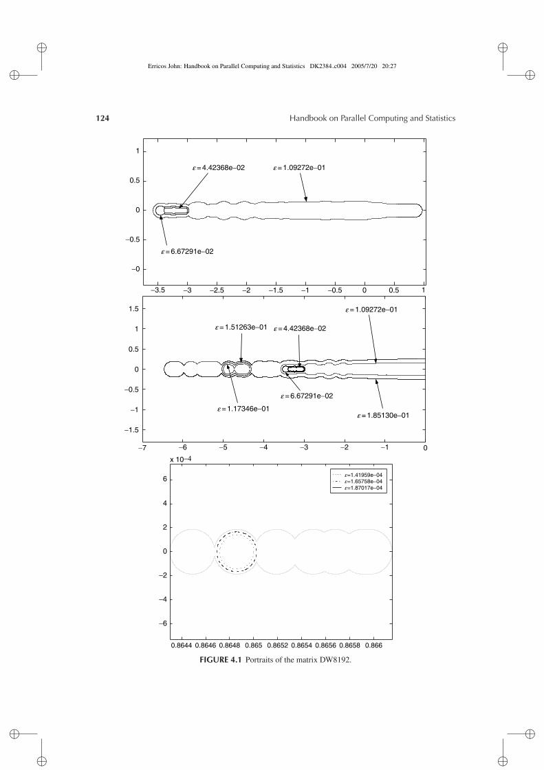
This proposition provides a criterion for deciding whether z belongs to ε(A). To representthe pseudospectrum graphically, one can define a grid in the complex region under considerationand compute σmin(A − zi j I ), for all the zi j determined by the grid. Although highly parallel, thisapproach involves a very high volume of operations. Presently, one prefers to use path-followingtechniques [11–13]. Section 4.5 describes one of these methods. For illustration, the pseudospec-trum of a matrix from the Matrix Market [14] test suite is displayed in Figure 4.1, where severalvalues of ε are shown.
In what follows, we present a selection of parallel algorithms for computing the SVD of denseand sparse matrices. For dense matrices, we restrict our survey to the Jacobi methods for ob-taining all the singular triplets, a class of methods not contained in ScaLAPACK [15, 16]. TheScaLAPACK (or Scalable LAPACK) library includes a subset of LAPACK routines redesigned fordistributed memory Multiple Instruction Multiple Data (MIMD) parallel computers. It is currentlywritten in a Single-Program-Multiple-Data style using explicit message passing for interprocessorcommunication. It assumes matrices are laid out in a two-dimensional block cyclic fashion. Theroutines of the library achieve respectable efficiency on parallel computers and the software is con-sidered to be robust. Some projects are under way, however, for making the use of ScaLAPACK inlarge-scale applications more user-friendly. Examples include, the PLAPACK project [17, 18], theOURAGAN project which is based on SCILAB [19], as well as projects based on MATLAB [20].None of these projects, however, provide all the capabilities of ScaLAPACK.
Whereas for sparse matrices, we concentrate our exposition on those schemes that obtain thesmallest singular triplets. We devote the last section to the vital primitives that help to assure therealization of high to performance on parallel computing platforms.
4.2 JACOBI METHODS FOR DENSE MATRICES
4.2.1 TWO-SIDED JACOBI SCHEME [2JAC]
Here, we consider the standard eigenvalue problem
Bx = λx (4.7)
where B is a real n × n-dense symmetric matrix. One of the best known methods for determiningall the eigenpairs of (4.7) was developed by the 19th century mathematician, Jacobi. We recall thatJacobi’s sequential method reduces the matrix B to the diagonal form by an infinite sequence ofplane rotations
Bk+1 = Uk BkU Tk , k = 1, 2, ...,
where B1 ≡ B, and Uk = Uk(i, j, θki j ) is a rotation of the (i, j)-plane where
ukii = uk
j j = ck = cos θki j and uk
i j = −ukji = sk = sin θk
i j .
The angle θki j is determined so that bk+1
i j = bk+1j i = 0, or
tan 2θki j = 2bk
i j
bkii − bk
j j
,
where |θki j | ≤ 1
4π .
�
�
Erricos John: Handbook on Parallel Computing and Statistics DK2384 c004 2005/7/20 20:27�
�
�
�
�
�
124 Handbook on Parallel Computing and Statistics
−3.5 −3 −2.5 −2 −1.5 −1 −0.5 0 0.5 1
e = 1.09272e−01
e = 6.67291e−02
e = 4.42368e−02
1
0.5
0
−0.5
−0
−7 −6 −5 −4 −3 −2 −1 0
−1.5
−1
−0.5
0
0.5
1
1.5 e = 1.09272e−01
e = 6.67291e−02
e = 4.42368e−02
e = 1.85130e−01e = 1.17346e−01
e = 1.51263e−01
0.8644 0.8646 0.8648 0.865 0.8652 0.8654 0.8656 0.8658 0.866
−6
−4
−2
0
2
4
6
x 10−4
e=1.41959e−04e=1.65758e−04e=1.87017e−04
FIGURE 4.1 Portraits of the matrix DW8192.

�
�
Erricos John: Handbook on Parallel Computing and Statistics DK2384 c004 2005/7/20 20:27�
�
�
�
�
�
Parallel Algorithms for the Singular Value Decomposition 125
For numerical stability, we determine the plane rotation by
ck = 1√1 + t2
k
and sk = cktk,
where tk is the smaller root (in magnitude) of the quadratic equation
t2k + 2αk tk − 1 = 0, αk = cot 2θk
i j .
Hence, tk may be written as
tk = sign αk
|αk | +√
1 + α2k
.
Each Bk+1 remains symmetric and differs from Bk only in rows and columns i and j , where themodified elements are given by
bk+1i i = bk
ii + tkbki j ,
bk+1j j = bk
j j − tkbki j ,
and
bk+1ir = ckbk
ir + skbkjr , (4.8)
bk+1jr = −skbk
ir + ckbkjr , (4.9)
in which r = i , j . If we represent Bk by
Bk = Dk + Ek + ETk , (4.10)
where Dk is diagonal and Ek is strictly upper triangular, then as k increases ‖ Ek ‖F approacheszero, and Bk approaches the diagonal matrix = diag (λ1, λ2, . . . , λn) (‖ · ‖F denotes the Frobe-nius norm). Similarly, the transpose of the product (Uk · · · U2U1) approaches a matrix whose j thcolumn is the eigenvector corresponding to λ j .
Several schemes are possible for selecting the sequence of elements bki j to be eliminated via
the plane rotations Uk . Unfortunately, Jacobi’s original scheme, which consists of sequentiallysearching for the largest off-diagonal element, is too time consuming for implementation on a mul-tiprocessor. Instead, a simpler scheme in which the off-diagonal elements (i, j) are annihilated inthe cycle fashion (1, 2), (1, 3), . . . , (1, n), (2, 3), . . . , (2, n), . . . , (n − 1, n) is usually adopted asits convergence is assured [21]. We refer to each sequence of n rotations as a sweep. Further-more, quadratic convergence for this sequential cyclic Jacobi scheme has been well documented(see Refs. [22, 23]). Convergence usually occurs within 6 to 10 sweeps, i.e., from 3n2 to 5n2 Jacobirotations.
A parallel version of this cyclic Jacobi algorithm is obtained by the simultaneous annihilationof several off-diagonal elements by a given Uk , rather than only one as is done in the serial version.For example, let B be of order 8 and consider the orthogonal matrix Uk as the direct sum of fourindependent plane rotations, where the ci ’s and si ’s for i = 1, 2, 3, 4 are simultaneously determined.An example of such a matrix is
Rk(1, 3) ⊕ Rk(2, 4) ⊕ Rk(5, 7) ⊕ Rk(6, 8),
�
�
Erricos John: Handbook on Parallel Computing and Statistics DK2384 c004 2005/7/20 20:27�
�
�
�
�
�
126 Handbook on Parallel Computing and Statistics
where Rk(i, j) is that rotation which annihilates the (i, j) off-diagonal element. If we considerone sweep to be a collection of orthogonal similarity transformations that annihilate the elementin each of the 1
2 n(n − 1) off-diagonal positions (above the main diagonal) only once, then fora matrix of order 8, the first sweep will consist of eight successive orthogonal transformationswith each one annihilating distinct groups of four elements simultaneously. For the remainingsweeps, the structure of each subsequent transformation Uk, k > 8, is chosen to be the same asthat of U j where j = 1 + (k − 1) mod 8. In general, the most efficient annihilation scheme
consists of (2r − 1) similarity transformations per sweep, where r =⌊
12 (n + 1)
⌋, in which
each transformation annihilates different⌊
12 n⌋
off-diagonal elements (see Ref. [24]). Althoughseveral annihilation schemes are possible, the Jacobi algorithm we present below utilizes an an-nihilation scheme which requires a minimal amount of indexing for computer implementation.Moreover, Luk and Park [25, 26] have demonstrated that various parallel Jacobi rotation orderingschemes are equivalent to the sequential row ordering scheme, and hence share the same conver-gence properties.
Algorithm [2JAC]Step 1: (Apply orthogonal similarity transformations via Uk for current sweep).
1. (a) For k = 1, 2, 3, . . . , n − 1 (serial loop)
simultaneously annihilate elements in position (i, j), where{i = 1, 2, 3, . . . ,
⌈12 (n − k)
⌉,
j = (n − k + 2) − i.
for k > 2,
{i = (n − k + 2), (n − k + 3), . . . , n −
⌊12 k⌋,
j = (2n − k + 2) − i.
(b) For k = n simultaneously annihilate elements in positions (i, j), where{i = 2, 3, . . . ,
⌈12 n⌉
j = (n + 2) − i
Step 2: (Convergence test).
1. (a) Compute ‖ Dk ‖F and ‖ Ek ‖F (see (4.10)).(b) If
‖ Ek ‖F
‖ Dk ‖F< tolerance, (4.11)
then stop. Otherwise, go to Step 1 to begin next sweep.
We note that this algorithm requires n similarity transformations per sweep for a dense realsymmetric matrix of order n (n may be even or odd). Each Uk is the direct sum of either
⌊ 12 n⌋
or⌊ 1
2 (n − 1)⌋
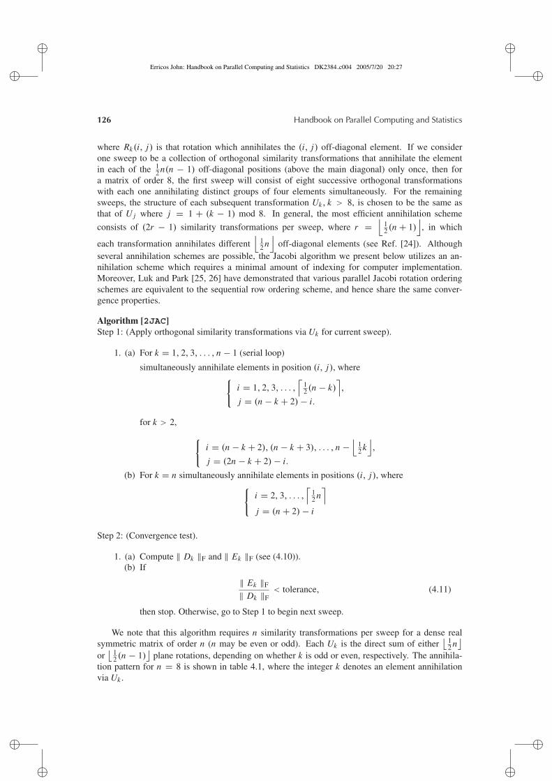
plane rotations, depending on whether k is odd or even, respectively. The annihila-tion pattern for n = 8 is shown in table 4.1, where the integer k denotes an element annihilationvia Uk .
�
�
Erricos John: Handbook on Parallel Computing and Statistics DK2384 c004 2005/7/20 20:27�
�
�
�
�
�
Parallel Algorithms for the Singular Value Decomposition 127
TABLE 4.1Annihilation Scheme for [2JAC]
x 7 6 5 4 3 2 1
x 5 4 3 2 1 8x 3 2 1 8 7
x 1 8 7 6x 7 6 5
x 5 4x 3
x
In the annihilation of a particular (i, j)-element in Step 1 above, we update the off-diagonalelements in rows and columns i and j as specified by (4.8) and (4.9). With regard to storagerequirements, it would be advantageous to modify only those row or column entries above the maindiagonal and utilize the guaranteed symmetry of Bk . However, if one wishes to take advantageof the vectorization that may be supported by the parallel computing platform, we disregard thesymmetry of Bk and operate with full vectors on the entirety of rows and columns i and j in (4.8)and (4.9), i.e., we are using a full matrix scheme. The product of the Uk’s, which eventually yieldsthe eigenvectors for B, is accumulated in a separate two-dimensional array by applying (4.8) and(4.9) to the n × n-identity matrix.
In Step 2, we monitor the convergence of the algorithm by using the ratio of the computednorms to measure the systematic decrease in the relative magnitudes of the off-diagonal elementswith respect to the relative magnitudes of the diagonal elements. For double precision accuracy inthe eigenvalues and eigenvectors, a tolerance of order 10−16 will suffice for Step 2(b). If we assumeconvergence (see Ref. [25]), this multiprocessor algorithm can be shown to converge quadraticallyby following the work of Wilkinson [23] and Henrici [27].
4.2.2 ONE-SIDED JACOBI SCHEME [1JAC]
Suppose that A is a real m × n-matrix with m � n and rank A = r . The SVD of A can be definedas
A = U�V T, (4.12)
where U TU = V TV = In and � = diag(σ1, . . . , σn), σi > 0 for 1 ≤ i ≤ r , σ j = 0 forj ≥ r + 1. The first r columns of the orthonormal matrix U and the orthogonal matrix V define theorthonormalized eigenvectors associated with the r nonzero eigenvalues of AAT or AT A.
As indicated in Ref. [28] for a ring of processors, using a method based on the one-sided iter-ative orthogonalization method of Hestenes (see also Ref. [29, 30]) is an efficient way to computethe decomposition (4.12). Luk [31] recommended this singular value decomposition scheme on theIlliac IV, and corresponding systolic algorithms associated with two-sided schemes have been pre-sented in Ref. [32, 33]. We now consider a few modifications to the scheme discussed in Ref. [28]for the determination of (4.12) on shared-memory multiprocessors, e.g., see Ref. [34].
�
�
Erricos John: Handbook on Parallel Computing and Statistics DK2384 c004 2005/7/20 20:27�
�
�
�
�
�
128 Handbook on Parallel Computing and Statistics
Our main goal is to determine the orthogonal matrix V = [V , W ], where V is n × r , so that
AV = Q = (q1, q2, . . . , qr ), (4.13)
andqT
i q j = σ 2i δi j ,
where the columns of A are orthogonal and δi j is the Kronecker-delta. Writing Q as
Q = U � with U TU = Ir , and � = diag(σ1, . . . , σr ),
thenA = U �V T.
We construct the matrix V via the plane rotations
(ai , a j )
[c −ss c
]= (ai , a j ), i < j,
so that
aTi a j = 0 and ‖ ai ‖2>‖ a j ‖2, (4.14)
where ai designates the i th column of matrix A. This is accomplished by choosing
c =[β + γ
2γ
]1/2
and s =[
α
2γc
], if β > 0, (4.15)
or
s =[γ − β
2γ
]1/2
and c =[
α
2γ s
], if β < 0, (4.16)
where α = 2aTi a j , β =‖ a j ‖2
2, and γ = (α2 + β2)1/2. Note that (4.14) requires the columns of Qto decrease in norm from left to right, and hence the resulting σi to be in monotonic nonincreasingorder. Several schemes can be used to select the order of the (i, j)-plane rotations. Following theannihilation pattern of the off-diagonal elements in the sequential Jacobi algorithm mentioned inSection 4.1, we could certainly orthogonalize the columns in the same cyclic fashion and thus per-form the one-sided orthogonalization serially. This process is iterative with each sweep consistingof 1
2 n(n − 1) plane rotations selected in cyclic fashion.By adopting the ordering of the annihilation scheme in [2JAC], we obtain a parallel version of
the one-sided Jacobi method for computing the singular value decomposition on a multiprocessor.For example, let n = 8 and m � n so that in each sweep of our one-sided Jacobi algorithm wesimultaneously orthogonalize pairs of columns of A (see Table 4.1). For example, for n = 8 we canorthogonalized the pairs (1,8), (2,7), (3,6), (4,5) simultaneously via postmultiplication by a matrixVi which consists of the direct sum of four plane rotations. In general, each Vk will have the sameform as Uk so that at the end of any particular sweep si we have
Vs1 = V1V2 · · · Vn,
and hence
V = Vs1 Vs2 · · · Vst , (4.17)
�
�
Erricos John: Handbook on Parallel Computing and Statistics DK2384 c004 2005/7/20 20:27�
�
�
�
�
�
Parallel Algorithms for the Singular Value Decomposition 129
where t is the number of sweeps required for convergence.
Algorithm [1JAC]Step 1: (Postmultiply matrix A by orthogonal matrix Vk for current sweep).
1. (a) Initialize the convergence counter, istop, to zero.(b) For k = 1, 2, 3, . . . , n − 1 (serial loop)
simultaneously orthogonalize the column pairs (i, j), where i and j are given by 1(a)in Step 1 of [2JAC], provided that for each (i, j) we have
(aTi a j )
2
(aTi ai )(aT
j a j )> tolerance, (4.18)
and i , j ∈ {k|k < kmin}, where kmin is the minimal column index k such that‖ ak ‖2
2< tolerance. Upon the termination of [1JAC], r = rank A = kmin. Note:if (4.18) is not satisfied for any particular pair (i, j), istop is incremented by 1 andthat rotation is not performed.
(c) For k = nsimultaneously orthogonalized the column pairs (i, j), where i and j are given by1(b) in Step 1 of [2JAC].
Step 2: (Convergence test).
If istop = 12 n(n − 1), then compute σi = √
(AT A)i i , i = 1, 2, . . . , kmin = r , and stop. Otherwise,go to beginning of Step 1 to start next sweep.
In the orthogonalization of columns in Step 1, we are implementing the plane rotations speci-fied by (4.15) and (4.16), and hence guaranteeing the ordering of column norms and singular valuesupon termination. Whereas [2JAC] must update rows and columns following each similarity trans-formation, [1JAC] performs only postmultiplication of A by each Vk and hence the plane rotation(i, j) changes only the elements in columns i and j of matrix A. The changed elements can berepresented by
ak+1i = cak
i + sakj , (4.19)
ak+1j = −sak
i + cakj , (4.20)
where ai denotes the i th column of matrix A, and c, s are determined by either (4.15) or (4.16).Since no row accesses are required and no columns are interchanged, one would expect good per-formance for this method on a machine which can apply vector operations to compute (4.19) and(4.20). Each processor is assigned one rotation and hence orthogonalizes one pair of the n columnsof matrix A.
Following the convergence test used in Ref. [30], in Step 2, we count the number of times thequantity
aTi a j
(aTi ai )(aT
j a j )(4.21)
falls, in any sweep, below a given tolerance. The algorithm terminates when the counter istopreaches 1
2 n(n − 1), the total number of column pairs, after any sweep. Upon termination, the firstr columns of the matrix A are overwritten by the matrix Q from (4.13) and hence the nonzero
�
�
Erricos John: Handbook on Parallel Computing and Statistics DK2384 c004 2005/7/20 20:27�
�
�
�
�
�
130 Handbook on Parallel Computing and Statistics
singular values σi can be obtained via the r square roots of the first r diagonal entries of AT A.The matrix U in (4.12), which contains the leading r , left singular vectors of the original matrix A,is readily obtained by column scaling of the resulting matrix A (now overwritten by Q = U�) bythe nonzero singular values σi . Similarly, the matrix V , which contains the right singular vectors ofthe original matrix A, is obtained as in (4.17) as the product of the orthogonal Vk’s. This productis accumulated in a separate two-dimensional array by applying the rotations specified by (4.19)and (4.20) to the n × n-identity matrix. It is important to note that the use of the ratio in (4.21)is preferable over the use of aT
i a j , since this dot-product is necessarily small for relatively smallsingular values.
Although our derivation of [1JAC] is concerned with the singular value decomposition of rec-tangular matrices, it is most effective for solving the eigenvalue problem in (4.7) for symmetricpositive definite matrices. If m = n = r , B is a positive definite matrix, and Q in (4.13) is anorthogonal matrix. Consequently, it is not difficult to show that{
σi = λi
xi = qiλi
,i = 1, 2, . . . , n,
where λi denotes the i th eigenvalue of B, xi the corresponding normalized eigenvector, and qi thei th column of matrix Q. If B is symmetric, but perhaps not positive definite, we can obtain its eigen-vectors by considering instead B + α I , where α is the smallest quantity that ensures definiteness ofB + α I , and retrieve the eigenvalues of B via Rayleigh quotients.
[1JAC] has two advantages over [2JAC]: (i) no row accesses are needed, and (ii) the matrix Qneed not be accumulated.
4.2.3 ALGORITHM [QJAC]
As discussed above, [1JAC] is certainly a viable candidate for computing the SVD (4.12) on mul-tiprocessors . However, for m × n-matrices A in which m � n, the problem complexity can bereduced if an initial orthogonal factorization of A is performed. One can then apply the one-sidedJacobi method, [1JAC], to the resulting upper-triangular matrix R (which may be singular) andobtain the decomposition (4.12). In this section, we present a multiprocessor method, QJAC, whichcan be quite effective for computing (4.12) on parallel machines.
Given the m × n-matrix A, where m � n, we perform a block generalization of Householder’sreduction for the orthogonal factorization
A = Q R, (4.22)
where Q is m × n-orthonormal matrix, and R is an n × n-upper-triangular matrix. The blockschemes of LAPACK are used for computing (4.22) to make use of vector–matrix, matrix–vector(BLAS2), and matrix–matrix (BLAS3) multiplication modules. The [1JAC] algorithm can then beused to obtain the SVD of the upper-triangular matrix R.
Hence, the SVD of an m × n-matrix (m � n) A (having rank r ) defined by
A = U�V T,
where U TU = V TV = Ir , and � = diag(σ1, . . . , σr ), σi > 0 for 1 ≤ i ≤ r , can be efficientlydetermined as follows:
Block Householder-Jacobi [QJAC]Step 1: Apply block Householder reduction via (3.6) to the matrix A to obtain the factorization
A = Q R, (4.23)
where Q is m × n with orthonormal columns, and R is upper triangular of order n.
�
�
Erricos John: Handbook on Parallel Computing and Statistics DK2384 c004 2005/7/20 20:27�
�
�
�
�
�
Parallel Algorithms for the Singular Value Decomposition 131
Step 2: Determine the SVD of the upper-triangular matrix via [1JAC],
R = U
[�0
]V T, (4.24)
where U and V are n × r -matrices having orthogonal columns (r ≡ rank A) and � = diag σi
contains the r nonzero singular values of A.
Step 3: Recover the left singular vectors ui of A by back-transforming the columns of U :
U = QU , (4.25)
where Q is the product of the Householder transformations applied in Step 1 and ui is the i thcolumn of U .
Note that in using [1JAC] for computing the SVD of R, we must iterate on a full n × n-matrix which is initially upper-triangular. This sacrifice in storage must be made to capitalize uponthe potential vectorization and parallelism inherent in [1JAC] on parallel machines with vectorprocessors.
Charlier et al. [35] demonstrate that an implementation of Kogbetliantz’s algorithm for com-puting the SVD of upper-triangular matrices is quite effective on a systolic array of processors.We recall that Kogbetliantz’s method for computing the SVD of a real square matrix A mirrors the[2JAC] method for symmetric matrices, in that the matrix A is reduced to the diagonal form by aninfinite sequence of plane rotations
Ak+1 = Uk Ak V Tk , k = 1, 2, . . . , (4.26)
where A1 ≡ A, and Vk = Vk(i, j, φki j ), Uk = Uk(i, j, θk
i j ) are orthogonal plane rotation matri-ces which deviate from In and Im , respectively, in the (i, i)-, ( j, j)-, (i, j)-, and ( j, i)-entries. Itfollows that Ak approaches the diagonal matrix � = diag(σ1, σ2, . . . , σn), where σi is the i thsingular value of A, and the products (Uk · · · U2U1), (Vk · · · V2V1) approach matrices whose i thcolumn is the respective left and right singular vector corresponding to σi . For the case whenthe σi ’s are not pathologically close, Paige and Van Dooren [36] have shown that the row (orcolumn) cyclic Kogbetliantz’s method ultimately converges quadratically. For triangular matrices,Charlier and Van Dooren [37] have demonstrated that Kogbetliantz’s algorithm converges quadrat-ically for those matrices having multiple or clustered singular values provided that singular valuesof the same cluster occupy adjacent diagonal position of Aν , where ν is the number of sweepsrequired for convergence. Even if we were to assume that R in (4.22) satisfies this conditionfor quadratic convergence of the parallel Kogbetliantz’s method in [36], the ordering of the ro-tations and subsequent row (or column) permutations needed to maintain the upper-triangular formis more efficient for systolic architectures than for shared-memory parallel machines. One clearadvantage of using [1JAC] is to determine the SVD of R lies in that the rotations defined by(4.15) or (4.16), as applied via the parallel ordering illustrated in Table 4.1, require no proces-sor synchronization among any set of the
⌊12 n⌋
or⌊
12 (n − 1)
⌋simultaneous plane rotations. The
convergence rate of [1JAC], however, does not necessarily match that of Kogbetliantz’salgorithm.
Let
Rk = Dk + Ek + ETk ,
�
�
Erricos John: Handbook on Parallel Computing and Statistics DK2384 c004 2005/7/20 20:27�
�
�
�
�
�
132 Handbook on Parallel Computing and Statistics
and
Sk = RTk Rk = Dk + Ek + ET
k , (4.27)
where Dk , Dk are diagonal matrices and Ek , Ek are strictly upper-triangular.Although we cannot guarantee quadratic convergence for [1JAC], we can always produce clus-
tered singular values on adjacent positions of Dk for any matrix A. If we monitor the magnitudesof the elements of Dk and Ek in (4.28) for successive values of k in [1JAC] (for clustered singularvalues), Sk will converge to a diagonal form through an intermediate block diagonal form, whereeach of the principal submatrices (positioned along Dk) has diagonal elements which comprise onecluster of singular values of A (see Refs. [34, 35]). Thus, after a particular number of critical sweepskcr, we obtain
Skcr =
T1T2
T3. . .
. . .
Tnc
(4.28)
so that the SVD of each Ti , i = 1, 2, . . . , nc, can be computed in parallel by either a Jacobi or Kog-betliantz’s method. Each symmetric matrix Ti will, in general, be dense of order qi , representingthe number of singular values of A contained in the i th cluster. Since the quadratic convergence ofKogbetliantz’s method for upper-triangular matrices [37] mirrors the quadratic convergence of thetwo-sided Jacobi method, [2JAC], for symmetric matrices having clustered spectra [38], we wouldobtain a faster global convergence for k > kcr if [2JAC], rather than [1JAC], were applied to eachof the Ti . Thus, a hybrid method consisting of an initial phase of several [1JAC] iterations followedby [2JAC] on the resulting subproblems would combine the optimal parallelism of [1JAC] and thefast convergence of the [2JAC] method. Of course, the difficulty in implementing such a methodlies in the determination of the critical number of sweeps kcr. We note that such a hybrid SVDmethod would be quite suitable for implementation on multiprocessors with hierarchical memorystructure and/or vector processors.
4.2.4 BLOCK-JACOBI ALGORITHMS
The above algorithms are well-suited for shared-memory computers. Although they can also beimplemented on distributed memory systems, their efficiency on such systems may suffer due tocommunication costs. To increase the granularity of the computation (i.e., to increase the numberof floating point operations between two communications), block algorithms are considered. Forone-sided algorithms, each processor is allocated a block of columns instead of a single column.The computation remains the same as discussed above with the ordering of the rotations within asweep is as given in Ref. [26].
For the two-sided version, the allocation manipulates two-dimensional blocks instead of sin-gle entries of the matrix. Some authors [39–41] propose a modification of the basic algorithm inwhich one annihilates, in each step, two off-diagonal blocks by performing a full SVD on a small-sized matrix. Good efficiencies are realized on distributed memory systems but this block strategyincreases the number of sweeps needed to reach convergence.
�
�
Erricos John: Handbook on Parallel Computing and Statistics DK2384 c004 2005/7/20 20:27�
�
�
�
�
�
Parallel Algorithms for the Singular Value Decomposition 133
We note that, parallel Jacobi algorithms can only surpass the speed of the bidiagonalizationschemes of ScaLAPACK when the number of processors available are much larger than the size ofthe matrix under consideration.
4.3 METHODS FOR LARGE AND SPARSE MATRICES
4.3.1 SPARSE STORAGES AND LINEAR SYSTEMS
When the matrix is large and sparse, a compact storage scheme must be considered. The principlebehind such storage schemes is to store only the nonzero entries and sometimes more data as in bandor profile storage schemes. For a more detailed presentation of various compact storage schemes,we refer for instance to Refs. [42, 43]. Here, we consider only the Compressed Sparse Row format(CSR) storage scheme.
Let us consider a sparse matrix A of order n with nz (denoted nz in algorithms) non zero entries.The CSR format is organized into three one-dimensional arrays:
array a(1:nz): contains all the nonzero entries of the matrix sorted by rows; within arow no special ordering is assumed although it is often preferable to sort the entries byincreasing column indices.
array ja(1:nz): contains all the column indices of the nonzero entries in the same orderas the order of the entries in array a.
array ia(1:n+1): , ia(i) (i = 1, . . . , n) is the index of the first nonzero entry of thei th row which is stored in array a and ia(n+1) is set to nz + 1.
The main procedures which use a matrix stored in that way are the multiplications of a matrix, A orAT, by a vector x ∈ R
n . The corresponding algorithms are:
ALGORITHM : y := y + A*x
for i = 1:n,for l = ia(i) : ia(i+1)-1,
y(i) = y(i) + a(l)*x(ja(l)) ;end ;
end ;
ALGORITHM : y := y + AT*x
for i = 1:n,for l = ia(i) : ia(i+1)-1,
y(ja(l)) = y(ja(l)) + a(l)*x(i) ;end ;
end
Solving linear systems which are defined by sparse matrices is not an easy task. One mayconsider direct methods, invariably consisting of matrix factorization, or consider iterative schemes.In direct solvers, care is needed to minimize the fill-in in the triangular factors, whereas in iterativemethods, adopting effective preconditioning techniques is vital for fast convergence.
It is usually admitted that direct methods are more robust but are economical only when thetriangular factors are not too dense, and when the size of the linear system is not too large. Re-ordering schemes are almost necessary to keep the level of fill-in as low as possible. Also, whilepivoting strategies for dense linear systems are relaxed to minimize fill-in, the most effective sparsefactorization schemes forbid the use of pivots below a given threshold. It is well known that theQR-factorization schemes, one of the most robust, is not used often in direct solvers as it suffersfrom a high level of fill-in. Such a high level of fill-in occurs because the upper-triangular fac-tor, R, is the transpose of the Cholesky factor of matrix AT A which is much more dense than theoriginal matrix A. Nevertheless, we shall see that this orthogonal factorization is a viable tool forcomputing the smallest singular value of sparse matrices. A survey of the state-of-the-art of sparse
�
�
Erricos John: Handbook on Parallel Computing and Statistics DK2384 c004 2005/7/20 20:27�
�
�
�
�
�
134 Handbook on Parallel Computing and Statistics
matrix factorization may be found in the following Refs. [42, 44–51]. Current efficient packagesfor LU-factorization include UMFPACK [52], SuperLU [53], and MUMPS [54].
When the order of the matrix is so large as to make the use of direct methods prohibitivelyexpensive in storage and time, one resorts to iterative solvers. Classic iterative solvers such as therelaxation schemes methods of Jacobi, Gauss Seidel, SOR, or SSOR, are easy to use but not aseffective as Krylov subspace methods. The latter class uses the matrix only through the proceduresof matrix–vector multiplications as defined above. Moreover, under certain conditions, Krylovsubspace schemes exhibit superlinear convergence. Often, however, Krylov subspace schemes aresuccessful only in conjunction with a preconditioning strategy. This is especially true for nonsym-metric ill-conditioned linear systems. Such preconditioners may be one of the above relaxationmethods, approximate factorizations or approximate inverses of the matrix of coefficients. A state-of-the-art survey of iterative solvers may be found in the following Refs. [43, 48, 55–58] or otherreferences therein. When the matrix is symmetric positive definite, a preconditioned conjugate gra-dient scheme (PCG) may be an optimal choice as an iterative solver [2]. For symmetric indefinitesystems, methods like SYMMLQ and MINRES [59] are adequate, but surprisingly PCG is oftenused with great success even though it may fail in theory. For nonsymmetric systems, the situationis less clear because available iterative schemes cannot combine minimization of the residual, atany given step, for a given norm within the Krylov subspace, and orthogonalizing it with respectto the same subspace for some scalar product. Therefore, two classes of methods arise. The mostpopular methods include GMRES [60], Bi-CGSTAB [61], QMR [62], and TFQMR [63].
Before presenting methods for computing the sparse SVD, we note that classical methods fordetermining the SVD of dense matrices: the Golub–Kahan–Reinsch method [64, 65] and Jacobi-like SVD methods [34, 66] are not viable for large sparse matrices. Because these methods applyorthogonal transformations (Householder or Givens) directly to the sparse matrix A, they incurexcessive fill-ins and thereby require tremendous amounts of storage. Another drawback to thesemethods is that they will compute all the singular triplets of A, and hence may be computationallywasteful when only a few of the smallest, or largest, singular triplets are desired. We demonstratehow canonical sparse symmetric eigenvalue problems can be used to (indirectly) compute the sparseSVD.
Since the computation of the smallest singular value is equivalent to computing an eigenvalueof a symmetric matrix, which is the augmented matrix or the matrix of the normal equations, inwhat follows we present methods that are specifically designed for such problems.
4.3.2 SUBSPACE ITERATION [SISVD]
Subspace iteration is perhaps one of the simplest algorithms used to solve large sparse eigenvalueproblems. As discussed in Ref. [67], subspace iteration may be viewed as a block generalizationof the classical power method. The basic version of subspace iteration was first introduced byBauer [68] and if adapted to the matrix
B = γ2 In − AT A, (4.29)
would involve forming the sequenceZk = Bk Z0,
where γ2 is chosen so that B is (symmetric) positive definite and Z0 = [z1, z2, . . . , zs] is an n × smatrix. If the column vectors, zi , are normalized separately (as done in the power method), thenthese vectors will converge to the dominant eigenvectors of B, which are also the right singularvectors corresponding to the smallest singular values of A. Thus, the columns of the matrix Zk
will progressively lose linear independence. To approximate the p-largest eigenpairs of B, Bauer
�
�
Erricos John: Handbook on Parallel Computing and Statistics DK2384 c004 2005/7/20 20:27�
�
�
�
�
�
Parallel Algorithms for the Singular Value Decomposition 135
demonstrated that linear independence among the zi ’s could be maintained via reorthogonalizationat each step, by a modified Gram–Schmidt procedure, for example. However, the convergence rateof the zi ’s to eigenvectors of B will only be linear.
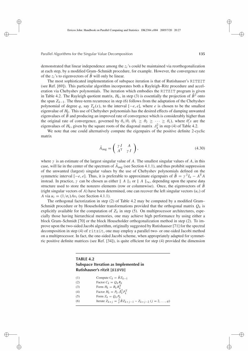
The most sophisticated implementation of subspace iteration is that of Rutishauser’s RITZIT(see Ref. [69]). This particular algorithm incorporates both a Rayleigh–Ritz procedure and accel-eration via Chebyshev polynomials. The iteration which embodies the RITZIT program is givenin Table 4.2. The Rayleigh quotient matrix, Hk , in step (3) is essentially the projection of B2 ontothe span Zk−1. The three-term recurrence in step (6) follows from the adaptation of the Chebyshevpolynomial of degree q, say Tq(x), to the interval [−e, e], where e is chosen to be the smallesteigenvalue of Hk . This use of Chebyshev polynomials has the desired effects of damping unwantedeigenvalues of B and producing an improved rate of convergence which is considerably higher thanthe original rate of convergence, governed by θs/θ1 (θ1 ≥ θ2 ≥ · · · ≥ θs), where θ ′
i s are theeigenvalues of Hk , given by the square roots of the diagonal matrix ∆2
k in step (4) of Table 4.2.We note that one could alternatively compute the eigenpairs of the positive definite 2-cyclic
matrix
Aaug =(
γ I AAT γ I
), (4.30)
where γ is an estimate of the largest singular value of A. The smallest singular values of A, in thiscase, will lie in the center of the spectrum of Aaug (see Section 4.1.1), and thus prohibit suppressionof the unwanted (largest) singular values by the use of Chebyshev polynomials defined on thesymmetric interval [−e, e]. Thus, it is preferable to approximate eigenpairs of B = γ 2 In − AT Ainstead. In practice, γ can be chosen as either ‖ A ‖1 or ‖ A ‖∞, depending upon the sparse datastructure used to store the nonzero elements (row or columnwise). Once, the eigenvectors of B(right singular vectors of A) have been determined, one can recover the left singular vectors (ui ) ofA via ui = (1/σi )Avi (see Section 4.1.1).
The orthogonal factorization in step (2) of Table 4.2 may be computed by a modified Gram–Schmidt procedure or by Householder transformations provided that the orthogonal matrix Qk isexplicitly available for the computation of Zk in step (5). On multiprocessor architectures, espe-cially those having hierarchical memories, one may achieve high performance by using either ablock Gram–Schmidt [70] or the block Householder orthogonalization method in step (2). To im-prove upon the two-sided Jacobi algorithm, originally suggested by Rutishauser [71] for the spectraldecomposition in step (4) of ritzit, one may employ a parallel two- or one-sided Jacobi methodon a multiprocessor. In fact, the one-sided Jacobi scheme, when appropriately adapted for symmet-ric positive definite matrices (see Ref. [34]), is quite efficient for step (4) provided the dimension
TABLE 4.2Subspace Iteration as Implemented inRutishauser’s ritzit [SISVD]
(1) Compute Ck = B Zk−1(2) Factor Ck = Qk Rk
(3) Form Hk = Rk RTk
(4) Factor Hk = Pk∆2k PT
k(5) Form Zk = Qk Pk
(6) Iterate Zk+ j = 2e B Zk+ j−1 − Zk+ j−2 ( j = 2, . . . , q)
�
�
Erricos John: Handbook on Parallel Computing and Statistics DK2384 c004 2005/7/20 20:27�
�
�
�
�
�
136 Handbook on Parallel Computing and Statistics
of the current subspace, s, is not too large. For larger subspaces, an optimized implementationof the classical EISPACK [72] pair, TRED2 and TQL2, or Cuppen’s algorithm as parallelized byDongarra and Sorensen [73] may be used in step (4).
The success of Rutishauser’s subspace iteration method using Chebyshev acceleration reliesupon the following strategy for delimiting the degree of the Chebyshev polynomial, Tq(x/e), onthe interval [−e, e], where e = θs (assuming s vectors carried and k = 1 initially), ξ1 = 0.04 andξ2 = 4:
qnew = min{2qold, q},where
q =
⎧⎪⎪⎪⎨⎪⎪⎪⎩
1, if θ1 < ξ1θs
2 × max
⎡⎣ ξ2
arccosh(
θsθ1
) , 1
⎤⎦ otherwise.
(4.31)
The polynomial degree of the current iteration is then taken to be q = qnew. It can easily be shownthat the strategy in (4.31) insures that
∥∥∥∥Tq
[θ1
θs
]∥∥∥∥2
= cosh
[q arccosh
(θ1
θs
)]≤ cosh(8) < 1500.
Although this bound has been quite successful for ritzit, we can easily generate several varia-tions of polynomial-accelerated subspace iteration schemes (SISVD) using a more flexible bound.Specifically, we consider an adaptive strategy for selecting the degree q in which ξ1 and ξ2 aretreated as control parameters for determining the frequency and the degree of polynomial accelera-tion, respectively. In other words, large (small) values of ξ1, inhibit (invoke) polynomial accelera-tion, and large (small) values of ξ2 yield larger (smaller) polynomial degrees when acceleration isselected. Correspondingly, the number of matrix–vector multiplications will increase with ξ2 andthe total number of iterations may well increase with ξ1. Controlling the parameters, ξ1 and ξ2,allows us to monitor the method’s complexity so as to maintain an optimal balance between dom-inating kernels (e.g., sparse matrix multiplication, orthogonalization, and spectral decomposition).We will demonstrate these controls in the polynomial acceleration-based trace minimization SVDmethod discussed in Section 4.3.4.
4.3.3 LANCZOS METHODS
4.3.3.1 The Single-Vector Lanczos Method [LASVD]
Other popular methods for solving large, sparse, symmetric eigenproblems originated from a methodattributed to Lanczos (1950). This method generates a sequence of tridiagonal matrices Tj with theproperty that the extremal eigenvalues of the j × j matrix Tj are progressively better estimates ofthe extremal eigenvalues of the original matrix. Let us consider the (m + n) × (m + n) 2-cyclicmatrix Aaug given in (4.3), where A is the m × n matrix whose singular triplets are sought. Also,let w1 be a randomly generated starting vector such that ‖w1‖2 = 1. For j = 1, 2, . . . , l define thecorresponding Lanczos matrices Tj using the following recursion [74]. Define β1 ≡ 0 and v0 ≡ 0,then for i = 1, 2, . . . , l define Lanczos vectors wi and scalars αi and βi+1 where
βi+1wi+1 = Aaugwi − αiwi − βiwi−1, and αi = wTi (Aaugwi − βiwi−1),
|βi+1| = ‖Aaugwi − αiwi − βiwi−1‖2.(4.32)
�
�
Erricos John: Handbook on Parallel Computing and Statistics DK2384 c004 2005/7/20 20:27�
�
�
�
�
�
Parallel Algorithms for the Singular Value Decomposition 137
For each j , the corresponding Lanczos matrix Tj is defined as a real symmetric, tridiagonalmatrix having diagonal entries αi (1 ≤ i ≤ j), and subdiagonal (superdiagonal) entries βi+1 (1 ≤i ≤ ( j − 1)), i.e.,
Tj ≡
⎛⎜⎜⎜⎜⎜⎜⎝
α1 β2β2 α2 β3
β3 · ·· · ·
· · β j
β j α j
⎞⎟⎟⎟⎟⎟⎟⎠
. (4.33)
By definition, the vectors αiwi and βiwi−1 in (4.32) are respectively, the orthogonal projectionsof Aaugwi onto the most recent wi and wi−1. Hence for each i , the next Lanczos vector wi+1 isobtained by orthogonalizing Aaugwi with respect to wi and wi−1. The resulting αi , βi+1 obtained inthese orthogonalizations, define the corresponding Lanczos matrices. If we rewrite (4.32) in matrixform, then for each j we have
AaugW j = W j Tj + β j+1w j+1e j , (4.34)
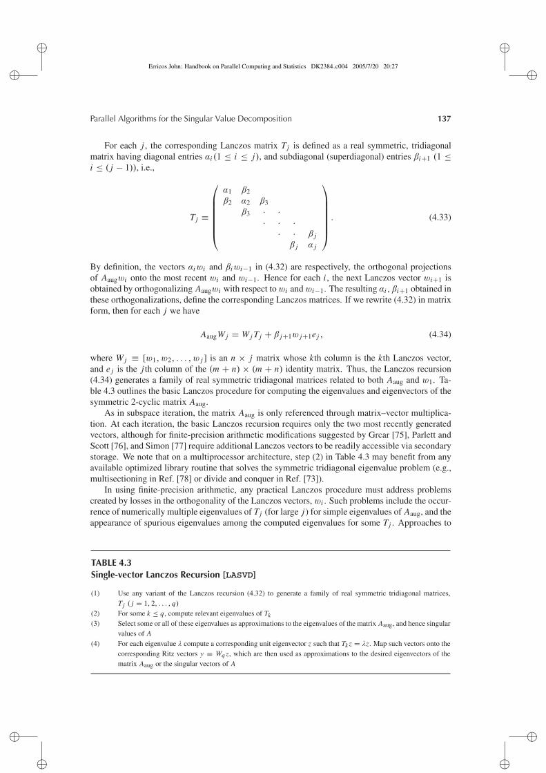
where W j ≡ [w1, w2, . . . , w j ] is an n × j matrix whose kth column is the kth Lanczos vector,and e j is the j th column of the (m + n) × (m + n) identity matrix. Thus, the Lanczos recursion(4.34) generates a family of real symmetric tridiagonal matrices related to both Aaug and w1. Ta-ble 4.3 outlines the basic Lanczos procedure for computing the eigenvalues and eigenvectors of thesymmetric 2-cyclic matrix Aaug.
As in subspace iteration, the matrix Aaug is only referenced through matrix–vector multiplica-tion. At each iteration, the basic Lanczos recursion requires only the two most recently generatedvectors, although for finite-precision arithmetic modifications suggested by Grcar [75], Parlett andScott [76], and Simon [77] require additional Lanczos vectors to be readily accessible via secondarystorage. We note that on a multiprocessor architecture, step (2) in Table 4.3 may benefit from anyavailable optimized library routine that solves the symmetric tridiagonal eigenvalue problem (e.g.,multisectioning in Ref. [78] or divide and conquer in Ref. [73]).
In using finite-precision arithmetic, any practical Lanczos procedure must address problemscreated by losses in the orthogonality of the Lanczos vectors, wi . Such problems include the occur-rence of numerically multiple eigenvalues of Tj (for large j) for simple eigenvalues of Aaug, and theappearance of spurious eigenvalues among the computed eigenvalues for some Tj . Approaches to
TABLE 4.3Single-vector Lanczos Recursion [LASVD]
(1) Use any variant of the Lanczos recursion (4.32) to generate a family of real symmetric tridiagonal matrices,Tj ( j = 1, 2, . . . , q)
(2) For some k ≤ q, compute relevant eigenvalues of Tk
(3) Select some or all of these eigenvalues as approximations to the eigenvalues of the matrix Aaug, and hence singularvalues of A
(4) For each eigenvalue λ compute a corresponding unit eigenvector z such that Tk z = λz. Map such vectors onto thecorresponding Ritz vectors y ≡ Wq z, which are then used as approximations to the desired eigenvectors of thematrix Aaug or the singular vectors of A
�
�
Erricos John: Handbook on Parallel Computing and Statistics DK2384 c004 2005/7/20 20:27�
�
�
�
�
�
138 Handbook on Parallel Computing and Statistics
deal with these problems range between two different extremes. The first involves total reorthogo-nalization of every Lanczos vector with respect to every previously generated vector [79]. The otherapproach accepts the loss of orthogonality and deals with these problems directly. Total reorthog-onalization is certainly one way of maintaining orthogonality, however, it will require additionalstorage and additional arithmetic operations. As a result, the number of eigenvalues which can becomputed is limited by the amount of available secondary storage. On the other hand, a Lanczosprocedure with no reorthogonalization needs only the two most recently generated Lanczos vectorsat each stage, and hence has minimal storage requirements. Such a procedure requires, however,the tracking [5] of the resulting spurious eigenvalues of Aaug (singular values of A) associated withthe loss of orthogonality in the Lanczos vectors, wi .
We employ a version of a single-vector Lanczos algorithm (4.32) equipped with a selective re-orthogonalization strategy, LANSO, designed by Parlett and Scott [76] and Simon [77]. This partic-ular method (LASVD) is primarily designed for the standard and generalized symmetric eigenvalueproblem. We simply apply it to either B = AT A or the 2-cyclic matrix Aaug defined in (4.3).
4.3.3.2 The Block Lanczos Method [BLSVD]
Here, we consider a block analog of the single-vector Lanczos method. Exploiting the structure ofthe matrix Aaug in (4.3), we can obtain an alternative form for the Lanczos recursion (4.32). If weapply the Lanczos recursion specified by (4.32) to Aaug with a starting vector u = (u, 0)T such that‖u‖2 = 1, then the diagonal entries of the real symmetric tridiagonal Lanzcos matrices generatedare all identically zero. The Lanzcos recursion in (4.32) reduces to the following: define u1 ≡ u,v0 ≡ 0, and β1 ≡ 0, then for i = 1, 2, . . . , k
β2ivi = ATui − β2i−1vi−1,β2i+1ui+1 = Avi − β2i ui .
(4.35)
The Lanczos recursion (4.35), however, can only compute the distinct singular values of anm × n matrix A and not their multiplicities. Following the block Lanczos recursion for the sparsesymmetric eigenvalue problem [80, 81], (4.35) can be represented in matrix form as
ATUk = Vk J Tk + Zk,
AVk = Uk Jk + Zk,(4.36)
where Uk = [u1, . . . , uk], Vk = [v1, . . . , vk], Jk is a k × k bidiagonal matrix with Jk[ j, j] = β2 j
and Jk[ j, j + 1] = β2 j+1, and Zk , Zk contain remainder terms. It is easy to show that the nonzerosingular values of Jk are the same as the positive eigenvalues of
Kk ≡(
O Jk
J Tk O
). (4.37)
For the block analog of (4.36), we make the simple substitutions
ui ↔ Ui , vi ↔ Vi ,
where Ui is m × b, Vi is n × b, and b is the current block size. The matrix Jk is now a upper blockbidiagonal matrix of order bk
Jk ≡
⎛⎜⎜⎜⎜⎜⎜⎝
S1 RT1
S2 RT2· ·
· ·· RT
k−1Sk
⎞⎟⎟⎟⎟⎟⎟⎠
, (4.38)
�
�
Erricos John: Handbook on Parallel Computing and Statistics DK2384 c004 2005/7/20 20:27�
�
�
�
�
�
Parallel Algorithms for the Singular Value Decomposition 139
where the Si ’s and Ri ’s are b × b upper-triangular matrices. If Ui ’s and Vi ’s form mutually orthog-onal sets of bk vectors so that Uk and Vk are orthonormal matrices, then the singular values of thematrix Jk will be identical to those of the original m×n matrix A. Given the upper block bidiagonalmatrix Jk , we approximate the singular triplets of A by first computing the singular triplets of Jk .To determine the left and right singular vectors of A from those of Jk , we must retain the Lanczosvectors of Uk and Vk . Specifically, if {σ (k)
i , y(k)i , z(k)
i } is the i th singular triplet of Jk , then the ap-proximation to the i th singular triplet of A is given by {σ (k)
i , Uk y(k)i , Vk z(k)
i }, where Uk y(k)i , Vk z(k)
iare the left and right approximate singular vectors, respectively. The computation of singular tripletsfor Jk requires two phases. The first phase reduces Jk to a bidiagonal matrix Ck having diagonalelements {α1, α2, . . . , αbk} and superdiagonal elements {β1, β2, . . . , βbk−1} via a finite sequence oforthogonal transformations (thus preserving the singular values of Jk). The second phase reducesCk to diagonal form by a modified QR-algorithm. This diagonalization procedure is discussed indetail in Ref. [65]. The resulting diagonalized Ck will yield the approximate singular values of A,whereas the corresponding left and right singular vectors are determined through multiplications byall the left and right transformations used in both phases of the SVD of Jk .
There are a few options for the reduction of Jk to the bidiagonal matrix, Ck . Golub et al.[82] advocated the use of either band Householder or band Givens methods which in effect chaseoff (or zero) elements on the diagonals above the first superdiagonal of Jk . In either reduction(bidiagonalization or diagonalization), the computations are primarily sequential and offer limiteddata locality or parallelism for possible exploitation on a multiprocessor. For this reason, we adoptthe single-vector Lanczos bidiagonalization recursion defined by (4.35) and (4.36) as our strategyfor reducing the upper block bidiagonal matrix Jk to the bidiagonal form (Ck), i.e.,
J Tk Q = PCT
k ,
Jk P = QCk,(4.39)
or
Jk p j = α j q j + β j−1q j−1,
J Tk q j = α j p j + β j p j+1,
(4.40)
where P ≡ {p1, p2, . . . , pbk} and Q ≡ {q1, q2, . . . , qbk} are orthonormal matrices of order bk×bk.The recursions in (4.40) require band matrix–vector multiplications which can be easily exploitedby optimized level-2 BLAS routines [83] now resident in optimized mathematical libraries on mosthigh-performance computers. For orthogonalization of the outermost Lanczos vectors, {Ui } and
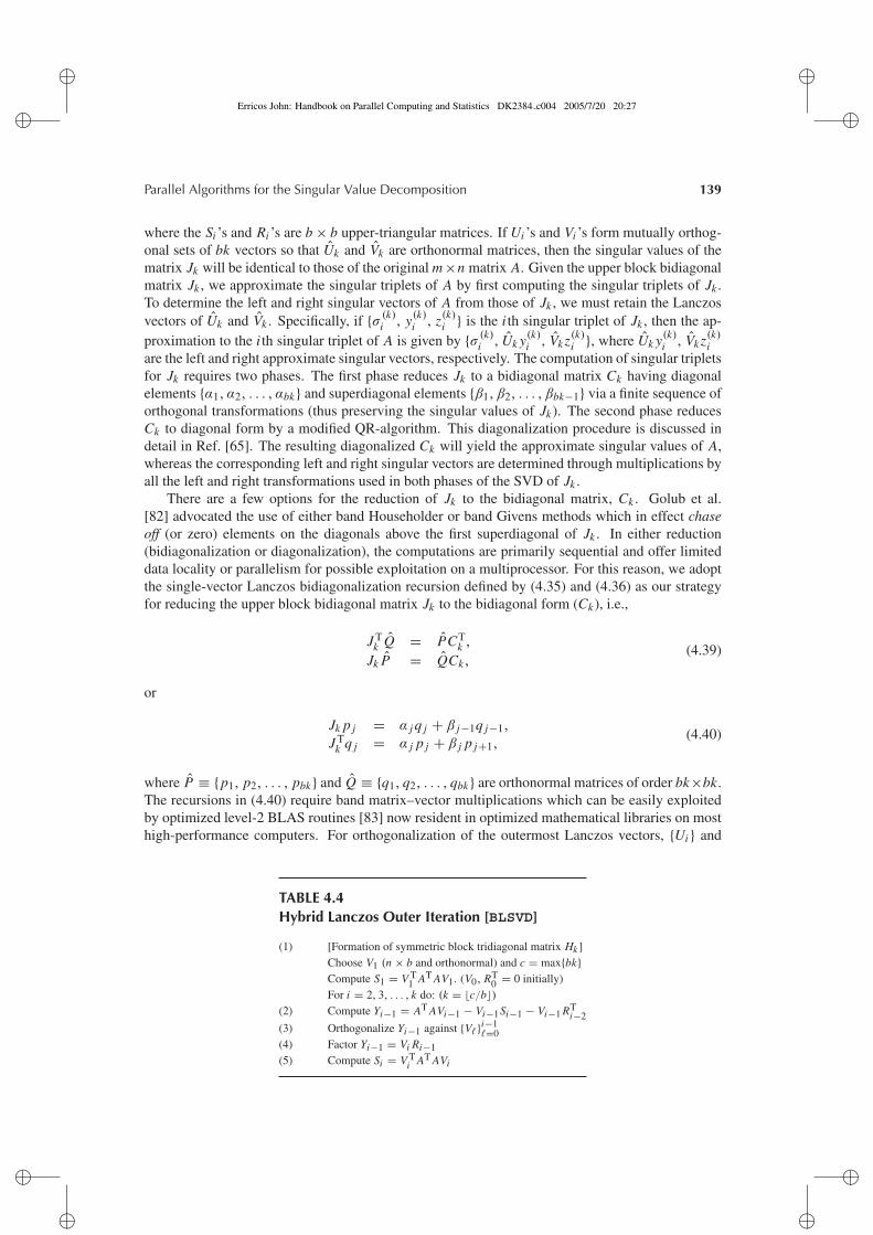
TABLE 4.4Hybrid Lanczos Outer Iteration [BLSVD]
(1) [Formation of symmetric block tridiagonal matrix Hk ]Choose V1 (n × b and orthonormal) and c = max{bk}Compute S1 = V T
1 AT AV1. (V0, RT0 = 0 initially)
For i = 2, 3, . . . , k do: (k = �c/b�)(2) Compute Yi−1 = AT AVi−1 − Vi−1Si−1 − Vi−1 RT
i−2(3) Orthogonalize Yi−1 against {V�}i−1
�=0(4) Factor Yi−1 = Vi Ri−1(5) Compute Si = V T
i AT AVi
�
�
Erricos John: Handbook on Parallel Computing and Statistics DK2384 c004 2005/7/20 20:27�
�
�
�
�
�
140 Handbook on Parallel Computing and Statistics
{Vi }, as well as the innermost Lanczos vectors, {pi } and {qi }, we have chosen to apply a completeor total reorthogonalization [79] strategy to insure robustness in our triplet approximations for thematrix A. This hybrid Lanczos approach which incorporates inner iterations of single-vector Lanc-zos bidiagonalization within the outer iterations of a block Lanczos SVD recursion is also discussedin Ref. [1].
As an alternative to the outer recursion defined by (4.36), which is derived from the equivalent 2-cyclic matrix Aaug, Table 4.4 depicts the simplified outer block Lanczos recursion for approximatingthe eigensystem of AT A. Combining the equations in (4.36), we obtain
AT AVk = Vk Hk,
where Hk = J Tk Jk is the k × k symmetric block tridiagonal matrix
Hk ≡
⎛⎜⎜⎜⎜⎜⎜⎝
S1 RT1
R1 S2 RT2
R2 · ·· · ·
· · RTk−1
Rk−1 Sk
⎞⎟⎟⎟⎟⎟⎟⎠
, (4.41)
having block size b. We then apply the block Lanczos recursion [79] in Table 4.4 for computing theeigenpairs of the n ×n symmetric positive definite matrix AT A. The tridiagonalization of Hk via aninner Lanczos recursion follows from simple modifications of (4.34). Analogous to the reductionof Jk in (4.38), the computation of eigenpairs of the resulting tridiagonal matrix can be performedvia a Jacobi or QR-based symmetric eigensolver.
As with the previous iterative SVD methods, we access the sparse matrices A and AT for thishybrid Lanczos method only through sparse matrix–vector multiplications. Some efficiency, how-ever, is gained in the outer (block) Lanczos iterations by the multiplication of b vectors rather thanby a single vector. These dense vectors may be stored in a fast local memory (cache) of a hier-archical memory-based architecture, and thus yield more effective data reuse. A stable variant ofGram–Schmidt orthogonalization [69], which requires efficient dense matrix–vector multiplication(level-2 BLAS) routines [83] or efficient dense matrix–matrix multiplication (level-3 BLAS) rou-tines [84], is used to produce the orthogonal projections of Yi (i.e., Ri−1) and Wi (i.e., Si ) onto V ⊥and U⊥, respectively, where U0 and V0 contain converged left and right singular vectors, respec-tively, and
V = (V0, V1, . . . , Vi−1) and U = (U0, U1, . . . , Ui−1).
4.3.4 THE TRACE MINIMIZATION METHOD [TRSVD]
Another candidate subspace method for the SVD of sparse matrices is based upon the trace mini-mization algorithm discussed in Ref. [85] for the generalized eigenvalue problem
H x = λGx, (4.42)
where H and G are symmetric and G is also positive definite. To compute the SVD of an m × nmatrix A, we initially replace H with Aaug as defined in (4.30) or set H = AT A. Since we need toonly consider equivalent standard symmetric eigenvalue problems, we simply define G = Im+n (orIn if H = AT A). Without loss of generality, let us assume that H = AT A, G = In and consider
�
�
Erricos John: Handbook on Parallel Computing and Statistics DK2384 c004 2005/7/20 20:27�
�
�
�
�
�
Parallel Algorithms for the Singular Value Decomposition 141
the associated symmetric eigensystem of order n. If Y is defined as the set of all n × p matrices Yfor which Y TY = Ip, then using the Courant–Fischer theorem (see Ref. [86]) we obtain
minY∈Y
trace(Y T HY ) =p∑
i=1
σn−i+1, (4.43)
where√
σi is a singular value of A, λi = σi is an eigenvalue of H , and σ1 ≥ σ2 ≥ · · · ≥ σn . Inother words, given an n × p matrix Y which forms a section of the eigenvalue problem
H z = λz, (4.44)
i.e.,
Y T HY = �, Y TY = Ip, (4.45)
� = diag(σn, σn−1, . . . , σn−p+1),
our trace minimization scheme [TRSVD] Ref. [85], see also [87], finds a sequence of iteratesYk+1 = F(Yk), where both Yk and Yk+1 form a section of (4.44), and have the property trace(Y T
k+1 HYk+1) < trace (Y Tk HYk). From (4.43), the matrix Y in (4.45) which minimizes trace(Y T HY )
is the matrix of H -eigenvectors associated with the p-smallest eigenvalues of the problem (4.44).As discussed in Ref. [85], F(Y ) can be chosen so that global convergence is assured. Moreover,(4.45) can be regarded as the quadratic minimization problem
minimize trace(Y T HY ) (4.46)
subject to the constraints
Y TY = Ip. (4.47)
Using Lagrange multipliers, this quadratic minimization problem leads to solving the (n + p) ×(n + p) system of linear equations
(H Yk
Y Tk 0
)(∆k
L
)=(
HYk
0
), (4.48)
so that Yk+1 ≡ Yk − ∆k will be an optimal subspace iterate.Since the matrix H is positive definite, one can alternatively consider the p-independent (paral-
lel) subproblems
minimize ((y(k)j − d(k)
j )T H(y(k)j − d(k)
j )) (4.49)
subject to the constraints
Y Td(k)j = 0, j = 1, 2, . . . , p,
where d(k)j = ∆ke j , e j the j th column of the identity, and Yk = [y(k)
1 , y(k)2 , . . . , y(k)
p ]. Thecorrections ∆k in this case are selected to be orthogonal to the previous estimates Yk , i.e., so that(see Ref. [88])
∆Tk Yk = 0.
�
�
Erricos John: Handbook on Parallel Computing and Statistics DK2384 c004 2005/7/20 20:27�
�
�
�
�
�
142 Handbook on Parallel Computing and Statistics
We then recast (4.48) as(H Yk
Y Tk 0
)(d(k)
jl
)=(
H y(k)j
0
), j = 1, 2, . . . , p, (4.50)
where l is a vector of order p reflecting the Lagrange multipliers.The solution of the p-systems of linear equations in (4.50) can be done in parallel by either a
direct or iterative solver. Since the original matrix A is assumed to be large, sparse and withoutany particular sparsity structure (pattern of nonzeros) we have chosen an iterative method (conju-gate gradient) for the systems in (4.50). As discussed in Refs. [1, 85], a major reason for usingthe conjugate gradient (CG) method for the solution of (4.50) stems from the ability to terminateCG iterations early without obtaining fully accurate corrections d(k)
j that are more accurate thanwarranted. In later stages, however, as Yk converges to the desired set of eigenvectors of B, oneneeds full accuracy in computing the correction matrix ∆k .
4.3.4.1 Polynomial Acceleration Techniques for [TRSVD]
The Chebyshev acceleration strategy used within subspace iteration (see Section 4.3.2), can also beapplied to [TRSVD]. However, to dampen unwanted (largest) singular values of A in this context,we must solve the generalized eigenvalue problem
x = 1
Pq(λ)Pq(H)x, (4.51)
where Pq(x) = Tq(x)+ε In , Tq(x) is the Chebyshev polynomial of degree q and ε is chosen so thatPq(H) is (symmetric) positive definite. The appropriate quadratic minimization problem similar to(4.49) here can be expressed as
minimize ((y(k)j − d(k)
j )T(y(k)j − d(k)
j )) (4.52)
subject to the constraintsY T Pq(H)d(k)
j = 0, j = 1, 2, . . . , p.
In effect, we approximate the smallest eigenvalues of H as the largest eigenvalues of the matrixPq(H) whose gaps are considerably larger than those of the eigenvalues of H .
Although the additional number of sparse matrix–vector multiplications associated with themultiplication by Pq(H) will be significant for high degrees q, the system of equations via Lagrangemultipliers in (4.50) becomes much easier to solve, i.e.,
(I Pq(H)Yk
Y Tk Pq(H) 0
)(d(k)
jl
)=(
y(k)j0
), j = 1, 2, . . . , p. (4.53)
It is easy to show that the updated eigenvector approximation, y(k+1)j , is determined by
y(k+1)j = y(k)
j − d(k)j = Pq(H)Yk[Y T
k P2q (H)Yk]−1Y T
k Pq(H)y(k)j .
Thus, we may not need to use an iterative solver for determining Yk+1 since the matrix [Y Tk P2
q (H)Yk]−1
is of relatively small order p. Using the orthogonal factorization
Pq(H)Yk = Q R,
we have[Y T
k P2q (H)Yk]−1 = R−T R−1,
where the polynomial degree, q, is determined by the strategy defined in Section 4.3.2.
�
�
Erricos John: Handbook on Parallel Computing and Statistics DK2384 c004 2005/7/20 20:27�
�
�
�
�
�
Parallel Algorithms for the Singular Value Decomposition 143
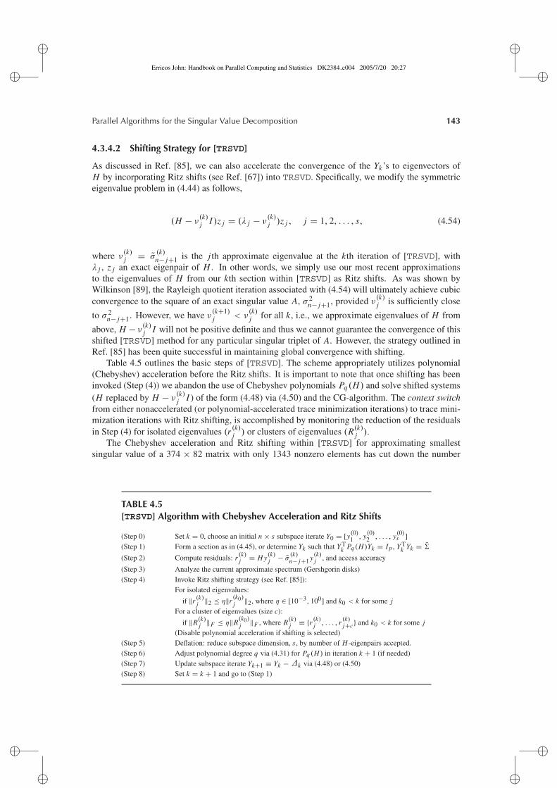
4.3.4.2 Shifting Strategy for [TRSVD]
As discussed in Ref. [85], we can also accelerate the convergence of the Yk’s to eigenvectors ofH by incorporating Ritz shifts (see Ref. [67]) into TRSVD. Specifically, we modify the symmetriceigenvalue problem in (4.44) as follows,
(H − ν(k)j I )z j = (λ j − ν
(k)j )z j , j = 1, 2, . . . , s, (4.54)
where ν(k)j = σ
(k)n− j+1 is the j th approximate eigenvalue at the kth iteration of [TRSVD], with
λ j , z j an exact eigenpair of H . In other words, we simply use our most recent approximationsto the eigenvalues of H from our kth section within [TRSVD] as Ritz shifts. As was shown byWilkinson [89], the Rayleigh quotient iteration associated with (4.54) will ultimately achieve cubicconvergence to the square of an exact singular value A, σ 2
n− j+1, provided ν(k)j is sufficiently close
to σ 2n− j+1. However, we have ν
(k+1)j < ν
(k)j for all k, i.e., we approximate eigenvalues of H from
above, H − ν(k)j I will not be positive definite and thus we cannot guarantee the convergence of this
shifted [TRSVD] method for any particular singular triplet of A. However, the strategy outlined inRef. [85] has been quite successful in maintaining global convergence with shifting.
Table 4.5 outlines the basic steps of [TRSVD]. The scheme appropriately utilizes polynomial(Chebyshev) acceleration before the Ritz shifts. It is important to note that once shifting has beeninvoked (Step (4)) we abandon the use of Chebyshev polynomials Pq(H) and solve shifted systems(H replaced by H − ν
(k)j I ) of the form (4.48) via (4.50) and the CG-algorithm. The context switch
from either nonaccelerated (or polynomial-accelerated trace minimization iterations) to trace mini-mization iterations with Ritz shifting, is accomplished by monitoring the reduction of the residualsin Step (4) for isolated eigenvalues (r (k)
j ) or clusters of eigenvalues (R(k)j ).
The Chebyshev acceleration and Ritz shifting within [TRSVD] for approximating smallestsingular value of a 374 × 82 matrix with only 1343 nonzero elements has cut down the number
TABLE 4.5[TRSVD] Algorithm with Chebyshev Acceleration and Ritz Shifts
(Step 0) Set k = 0, choose an initial n × s subspace iterate Y0 = [y(0)1 , y(0)
2 , . . . , y(0)s ]
(Step 1) Form a section as in (4.45), or determine Yk such that Y Tk Pq (H)Yk = Ip , Y T
k Yk = �
(Step 2) Compute residuals: r (k)j = H y(k)
j − σ(k)n− j+1 y(k)
j , and access accuracy
(Step 3) Analyze the current approximate spectrum (Gershgorin disks)(Step 4) Invoke Ritz shifting strategy (see Ref. [85]):
For isolated eigenvalues:
if ‖r (k)j ‖2 ≤ η‖r
(k0)j ‖2, where η ∈ [10−3, 100] and k0 < k for some j
For a cluster of eigenvalues (size c):
if ‖R(k)j ‖F ≤ η‖R
(k0)j ‖F , where R(k)
j ≡ {r (k)j , . . . , r (k)
j+c} and k0 < k for some j(Disable polynomial acceleration if shifting is selected)
(Step 5) Deflation: reduce subspace dimension, s, by number of H -eigenpairs accepted.(Step 6) Adjust polynomial degree q via (4.31) for Pq (H) in iteration k + 1 (if needed)(Step 7) Update subspace iterate Yk+1 ≡ Yk − ∆k via (4.48) or (4.50)(Step 8) Set k = k + 1 and go to (Step 1)
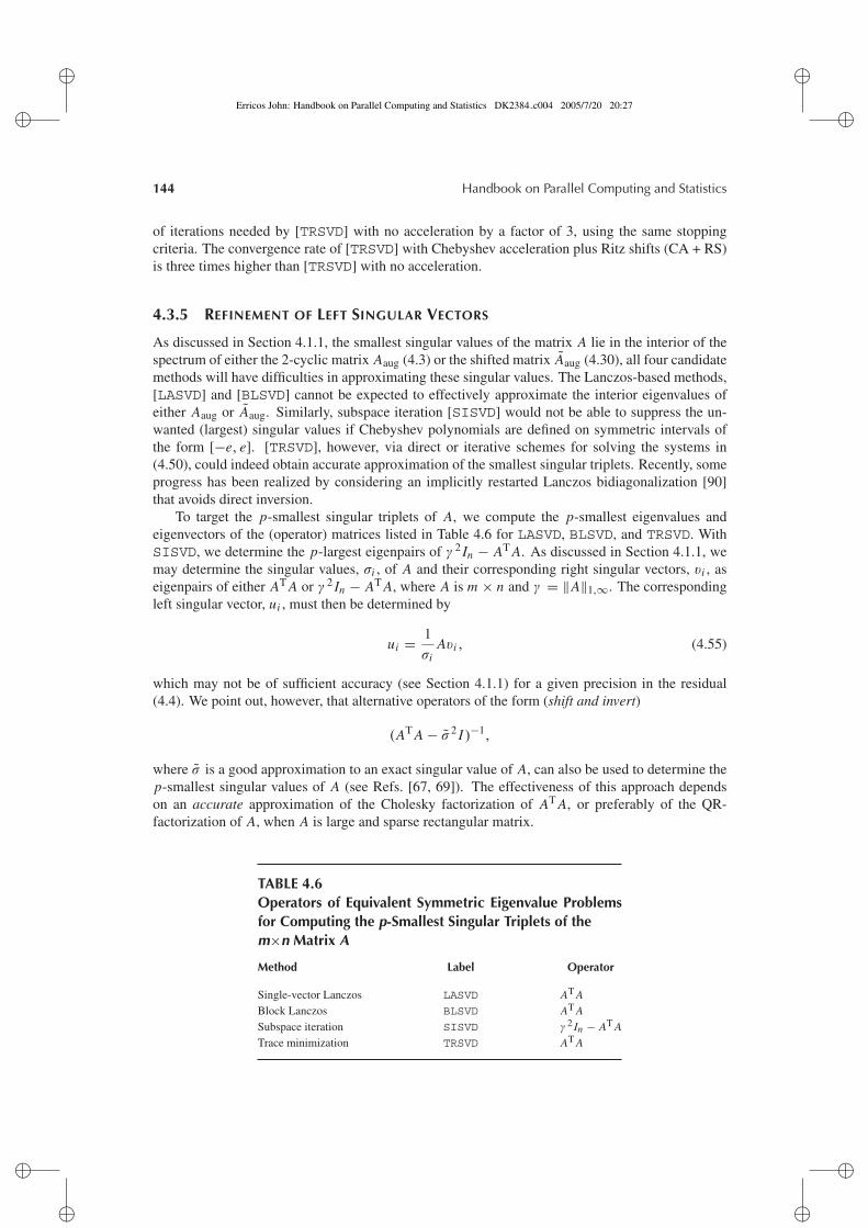
�
�
Erricos John: Handbook on Parallel Computing and Statistics DK2384 c004 2005/7/20 20:27�
�
�
�
�
�
144 Handbook on Parallel Computing and Statistics
of iterations needed by [TRSVD] with no acceleration by a factor of 3, using the same stoppingcriteria. The convergence rate of [TRSVD] with Chebyshev acceleration plus Ritz shifts (CA + RS)is three times higher than [TRSVD] with no acceleration.
4.3.5 REFINEMENT OF LEFT SINGULAR VECTORS
As discussed in Section 4.1.1, the smallest singular values of the matrix A lie in the interior of thespectrum of either the 2-cyclic matrix Aaug (4.3) or the shifted matrix Aaug (4.30), all four candidatemethods will have difficulties in approximating these singular values. The Lanczos-based methods,[LASVD] and [BLSVD] cannot be expected to effectively approximate the interior eigenvalues ofeither Aaug or Aaug. Similarly, subspace iteration [SISVD] would not be able to suppress the un-wanted (largest) singular values if Chebyshev polynomials are defined on symmetric intervals ofthe form [−e, e]. [TRSVD], however, via direct or iterative schemes for solving the systems in(4.50), could indeed obtain accurate approximation of the smallest singular triplets. Recently, someprogress has been realized by considering an implicitly restarted Lanczos bidiagonalization [90]that avoids direct inversion.
To target the p-smallest singular triplets of A, we compute the p-smallest eigenvalues andeigenvectors of the (operator) matrices listed in Table 4.6 for LASVD, BLSVD, and TRSVD. WithSISVD, we determine the p-largest eigenpairs of γ 2 In − AT A. As discussed in Section 4.1.1, wemay determine the singular values, σi , of A and their corresponding right singular vectors, vi , aseigenpairs of either AT A or γ 2 In − AT A, where A is m × n and γ = ‖A‖1,∞. The correspondingleft singular vector, ui , must then be determined by
ui = 1
σiAvi , (4.55)
which may not be of sufficient accuracy (see Section 4.1.1) for a given precision in the residual(4.4). We point out, however, that alternative operators of the form (shift and invert)
(AT A − σ 2 I )−1,
where σ is a good approximation to an exact singular value of A, can also be used to determine thep-smallest singular values of A (see Refs. [67, 69]). The effectiveness of this approach dependson an accurate approximation of the Cholesky factorization of AT A, or preferably of the QR-factorization of A, when A is large and sparse rectangular matrix.
TABLE 4.6Operators of Equivalent Symmetric Eigenvalue Problemsfor Computing the p-Smallest Singular Triplets of them×n Matrix A
Method Label Operator
Single-vector Lanczos LASVD AT ABlock Lanczos BLSVD AT A
Subspace iteration SISVD γ 2 In − AT A
Trace minimization TRSVD AT A
�
�
Erricos John: Handbook on Parallel Computing and Statistics DK2384 c004 2005/7/20 20:27�
�
�
�
�
�
Parallel Algorithms for the Singular Value Decomposition 145
For [LASVD], we simply define Aaug = AT A in (4.32) and apply the strategy outlined in Table4.3. For [SISVD] we make the substitution Aaug = γ 2 In − AT A for (4.30) and apply the methodin Table 4.2. Similarly, we solve the generalized eigenvalue problem in (4.44) with
H = AT A, G = In,
and apply the strategy in Table 4.5 for the appropriate [TRSVD] method. Here, we do not requirethe shift, γ 2, because the trace minimization will converge to the smallest eigenvalues of AT A (andhence squares of singular values of A) by default. For [BLSVD], we combine the equations in (4.36)and obtain
AT AVk = Vk Hk + Zk,
where Hk = J Tk Jk is the k × k symmetric block tridiagonal matrix in (4.41), with the n × k matrix
Zk containing the remainder terms. The appropriate block Lanczos (outer) recursion is then givenby Table 4.4.
Having determined approximate singular values, σi , and corresponding right singular vectors,vi , to a user-specified tolerance for the residual
ri = AT Avi − σ 2i vi , (4.56)
we must then obtain an approximation to the corresponding left singular vector, ui , via (4.55). Asmentioned in Section 4.1.1, it is quite possible that square roots of the approximate eigenvaluesof either AT A or γ 2 In − AT A will be poor approximations to exact singular values of A whichare extremely small. This phenomenon, of course, will lead to poor approximations to the leftsingular vectors. Even if σi (computed by any of the four methods) is an acceptable singular valueapproximation, the residual corresponding to the singular triplet {σi , ui , vi }, defined by (4.4), willbe bounded by
‖ri‖2 ≤ ‖ri‖2/[σi (‖ui‖22 + ‖vi‖2
2)12 ], (4.57)
where ri is the residual given in (4.56) for the symmetric eigenvalue problem for AT A or (γ 2 In −AT A). Scaling by σi can easily lead to significant loss of accuracy in estimating the triplet residualnorm, ‖ri‖2, especially when σi approaches the machine unit roundoff error, µ.
One remedy is to refine the initial approximation of the left singular vector via (inverse iteration)
AATu(k)i+1 = σ 2
i u(k)i , (4.58)
where u(0)i ≡ ui from (4.55). Since AAT is symmetric semidefinite, direct methods developed by
Aasen [91], Bunch and Kaufman [92], or Parlett and Reid [93] could be used in each step of (4.58)if AAT is explicitly formed. With regard to iterative methods, the SYMMLQ algorithm developed byPaige and Saunders [94] can be used to solve these symmetric indefinite systems of equations. Asan alternative, we consider the following equivalent eigensystem for the SVD of an m ×n matrix A.
(γ In AT
A γ Im
)(vi
ui
)= (γ + σi )
(vi
ui
), (4.59)
where {σi , ui , vi } is the i th singular triplet of A and
γ = min[1, max{σi }]. (4.60)
�
�
Erricos John: Handbook on Parallel Computing and Statistics DK2384 c004 2005/7/20 20:27�
�
�
�
�
�
146 Handbook on Parallel Computing and Statistics
One possible refinement recursion (inverse iteration) is thus given by
(γ In AT
A γ Im
)(v
(k+1)i
u(k+1)i
)= (γ + σi )
(v
(k)i
u(k)i
), (4.61)
By applying block Gaussian elimination to (4.61) we obtain a more optimal form (reduced system)of the recursion(
γ In AT
0 γ Im − 1γ AAT
)(v
(k+1)i
u(k+1)i
)= (γ + σi )
(v
(k)i
u(k)i − 1
γ Av(k)i
). (4.62)
Our iterative refinement strategy for an approximate singular triplet of A, {σi , ui , vi }, is then definedby the last m equations of (4.62), i.e.,
(γ Im − 1
γAAT
)u(k+1)
i = (γ + σi )
(u(k)
i − 1
γAvi
), (4.63)
where the superscript k is dropped from vi , since we refine only our left singular vector approxima-tion, ui . If u(0)
i ≡ ui from (4.59), then (4.63) can be rewritten as(
γ Im − 1
γAAT
)u(k+1)
i = (γ − σ 2i /γ )u(k)
i , (4.64)
with (normalization)u(k+1)
i = u(k+1)i /‖u(k+1)
i ‖2.
It is easy to show that the left-hand-side matrix in (4.63) is symmetric positive definite provided(4.60) holds. Accordingly, we may use parallel conjugate gradient iterations to refine each singulartriplet approximation. Hence, the refinement procedure outlined in Table 4.6 may be consideredas a black box procedure to follow the eigensolution of AT A or γ 2 In − AT A by any one of ourfour candidate methods for the sparse SVD. The iterations in Step (3) of the refinement scheme inTable 4.7 terminate once the norms of the residuals of all p approximate singular triplets (‖ri‖2)fall below a user-specified tolerance or after kmax iterations.
(α In + β AT A)ui = (α + βσ 2i ), vi
TABLE 4.7Refinement Procedure for the Left SingularVector Approximations Obtained Via Scaling
(1) Solve eigensystems of the form i = 1, 2, . . . , p, whereα = 0 and β = 1 for LASVD, BLSVD, and TRSVD, orα = γ 2 > σ 2
max and β = −1 for SISVD
(2) Define u(0)i ≡ 1
σiAvi , i = 1, 2, . . . , p
(3) For k = 0, 1, 2, . . . (until ‖ri ‖2 ≤ tolerance or k ≥kmax)
Solve(γ Im − 1
γ AAT)
u(k+1)i = (γ − σ 2
i /γ )u(k)i ,
i = 1, 2, . . . , p
Set u(k+1)i = u(k+1)
i /‖u(k+1)i ‖2
�
�
Erricos John: Handbook on Parallel Computing and Statistics DK2384 c004 2005/7/20 20:27�
�
�
�
�
�
Parallel Algorithms for the Singular Value Decomposition 147
SUMMARY
In this work, we demonstrated that a trace minimization strategy [TRSVD] using Chebyshev ac-celeration, Ritz shifting, and an iterative refinement method for improving left singular vector ap-proximations, can be quite economical and robust when computing several of the smallest singulartriplets of sparse matrices arising from a variety of applications. A single-vector Lanczos method[LASVD] can be quite competitive in speed compared to [TRSVD] at the risk of missing some ofthe desired triplets due to parameter selection difficulties. Whereas [TRSVD] is effective in achiev-ing high accuracy in approximating all the desired singular triplets. [LASVD] is acceptable onlywhen moderate to low accurate triplets are needed. A subspace iteration-based method [SISVD]using Chebyshev acceleration performed poorly for clustered singular values when polynomials ofrelatively high degree are used. Typically, this scheme requires less memory than the other threemethods. A block Lanczos SVD method [BLSVD], on the other hand, is quite robust for obtainingall the desired singular triplets at the expense of large memory requirements. The use of alternativereorthogonalization strategies could be a remedy for this difficulty. Finally, we have proposed a hy-brid [TRSVD] method which circumvents the potential loss of accuracy when solving eigensystemsof AT A.
4.3.6 THE DAVIDSON METHODS
4.3.6.1 General Framework of the Methods
In 1975, Davidson [95] introduced a method for computing the smallest eigenvalues of theSchrodinger operator. Later, the method was generalized in two papers by Morgan and Scott [96]and Crouzeix et al. [97] in which the convergence of the method is proved. More recently, anotherversion of the algorithm, under the name Jacobi–Davidson, was introduced in Ref. [98]. We presenthere a general framework for the class of Davidson methods, and point out how the various versionsdiffer from one another. We should point out that for symmetric eigenvalue problems, the David-son method version in Ref. [98] is strongly related to the trace minimization scheme discussed inSection 4.3.4, see Refs. [85, 99]. All versions of the Davidson method may be regarded as variousforms of preconditioning the basic Lanczos method. To illustrate this point, let us consider a sym-metric matrix A ∈ R
n×n . Both classes of algorithms generate, at some iteration k, an orthonormalbasis Vk = [v1, ..., vk] of a k-dimensional subspace Vk of R
n×n . In the Lanczos algorithm, Vk isa Krylov subspace, but for Davidson methods, this is not the case. In both classes, however, theinteraction matrix is given by the symmetric matrix Hk = Vk
T AVk ∈ Rk×k . Likely with the Lanc-
zos method, the goal is to obtain Vk such that some eigenvalues of Hk are good approximations ofsome eigenvalues of A: if (λ, y) is an eigenpair of Hk , then it is expected that the Ritz pair (λ, x),where x = Vk y, is a good approximation of an eigenpair of A. Note that this occurs only for someeigenpairs of Hk and at convergence.
Davidson methods differ from Lanczos in the definition of the new direction w which willbe incorporated in the subspace Vk to obtain Vk+1. For Lanczos schemes the vector w is givenby w = Avk , whereas for Davidson methods, a local improvement of the direction of the Ritzvector towards the sought after eigenvector is obtained by a quasi-Newton step (similar to the traceminimization scheme in Refs. [85, 99]). In Lanczos, the following vector vk+1 is computed by thethree-term recursion, if reorthogonalization is not considered, whereas in Davidson methods, thenext vector is obtained by reorthogonalizing w with respect to Vk . Moreover, in this case, the matrixHk is no longer tridiagonal. Therefore, one iteration of Davidson methods involves more arithmeticoperations than the basic Lanczos scheme; it is at least as expensive as a Lanczos scheme with fullreorthogonalization. Moreover, the basis Vk must be stored which implies the need for limiting the
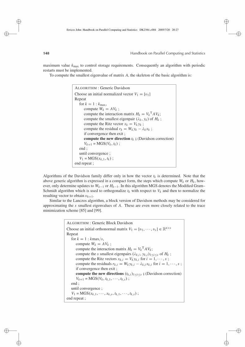
�
�
Erricos John: Handbook on Parallel Computing and Statistics DK2384 c004 2005/7/20 20:27�
�
�
�
�
�
148 Handbook on Parallel Computing and Statistics
maximum value kmax to control storage requirements. Consequently an algorithm with periodicrestarts must be implemented.
To compute the smallest eigenvalue of matrix A, the skeleton of the basic algorithm is:
ALGORITHM : Generic Davidson
Choose an initial normalized vector V1 = [v1]Repeat
for k = 1 : kmax,compute Wk = AVk ;compute the interaction matrix Hk = Vk
T AVk ;compute the smallest eigenpair (λk, yk) of Hk ;compute the Ritz vector xk = Vk yk ;compute the residual rk = Wk yk − λk xk ;if convergence then exit ;compute the new direction tk ; (Davidson correction)Vk+1 = MGS(Vk, tk) ;
end ;until convergence ;V1 = MGS(xk,1, tk) ;
end repeat ;
Algorithms of the Davidson family differ only in how the vector tk is determined. Note that theabove generic algorithm is expressed in a compact form, the steps which compute Wk or Hk , how-ever, only determine updates to Wk−1 or Hk−1. In this algorithm MGS denotes the Modified Gram–Schmidt algorithm which is used to orthogonalize tk with respect to Vk and then to normalize theresulting vector to obtain vk+1.
Similar to the Lanczos algorithm, a block version of Davidson methods may be considered forapproximating the s smallest eigenvalues of A. These are even more closely related to the traceminimization scheme [85] and [99].
ALGORITHM : Generic Block Davidson
Choose an initial orthonormal matrix V1 = [v1, · · · , vs] ∈ Rn×s
Repeatfor k = 1 : kmax/s,
compute Wk = AVk ;compute the interaction matrix Hk = Vk
T AVk ;compute the s smallest eigenpairs (λk,i , yk,i )1≤i≤s of Hk ;compute the Ritz vectors xk,i = Vk yk,i for i = 1, · · · , s ;compute the residuals rk,i = Wk yk,i − λk,i xk,i for i = 1, · · · , s ;if convergence then exit ;compute the new directions (tk,i )1≤i≤s ; (Davidson correction)Vk+1 = MGS(Vk, tk,1, · · · , tk,s) ;
end ;until convergence ;V1 = MGS(xk,1, · · · , xk,s, tk,1, · · · , tk,s) ;
end repeat ;
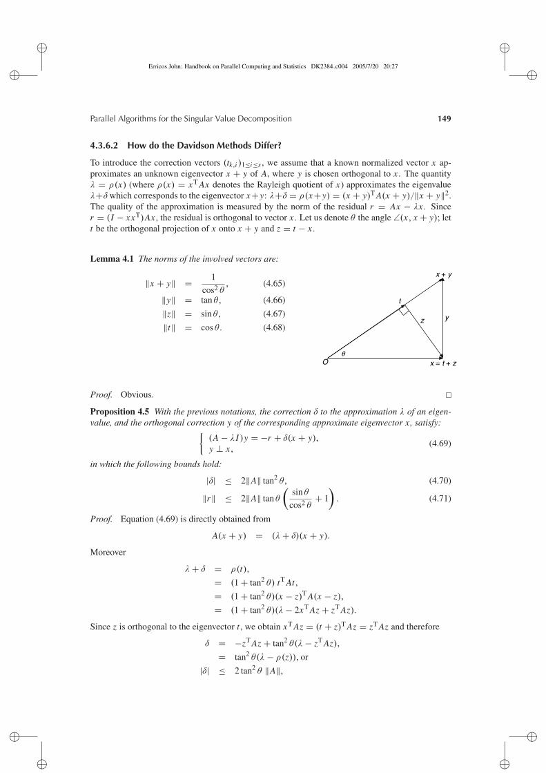
�
�
Erricos John: Handbook on Parallel Computing and Statistics DK2384 c004 2005/7/20 20:27�
�
�
�
�
�
Parallel Algorithms for the Singular Value Decomposition 149
4.3.6.2 How do the Davidson Methods Differ?
To introduce the correction vectors (tk,i )1≤i≤s , we assume that a known normalized vector x ap-proximates an unknown eigenvector x + y of A, where y is chosen orthogonal to x . The quantityλ = ρ(x) (where ρ(x) = xT Ax denotes the Rayleigh quotient of x) approximates the eigenvalueλ+δ which corresponds to the eigenvector x+y: λ+δ = ρ(x+y) = (x + y)T A(x + y)/‖x + y‖2.The quality of the approximation is measured by the norm of the residual r = Ax − λx . Sincer = (I − xxT)Ax , the residual is orthogonal to vector x . Let us denote θ the angle ∠(x, x + y); lett be the orthogonal projection of x onto x + y and z = t − x .
Lemma 4.1 The norms of the involved vectors are:
‖x + y‖ = 1
cos2 θ, (4.65)
‖y‖ = tan θ, (4.66)
‖z‖ = sin θ, (4.67)
‖t‖ = cos θ. (4.68)
t
y
x = t + z
z
x + y
qO
Proof. Obvious.
Proposition 4.5 With the previous notations, the correction δ to the approximation λ of an eigen-value, and the orthogonal correction y of the corresponding approximate eigenvector x, satisfy:{
(A − λI )y = −r + δ(x + y),y ⊥ x,
(4.69)
in which the following bounds hold:
|δ| ≤ 2‖A‖ tan2 θ, (4.70)
‖r‖ ≤ 2‖A‖ tan θ
(sin θ
cos2 θ+ 1
). (4.71)
Proof. Equation (4.69) is directly obtained from
A(x + y) = (λ + δ)(x + y).
Moreover
λ + δ = ρ(t),
= (1 + tan2 θ) tT At,
= (1 + tan2 θ)(x − z)T A(x − z),
= (1 + tan2 θ)(λ − 2xT Az + zT Az).
Since z is orthogonal to the eigenvector t , we obtain xT Az = (t + z)T Az = zT Az and therefore
δ = −zT Az + tan2 θ(λ − zT Az),
= tan2 θ(λ − ρ(z)), or
|δ| ≤ 2 tan2 θ ‖A‖,
�
�
Erricos John: Handbook on Parallel Computing and Statistics DK2384 c004 2005/7/20 20:27�
�
�
�
�
�
150 Handbook on Parallel Computing and Statistics
which proves (4.70). Bound (4.71) is a straight consequence of relations (4.69), (4.66),and (4.70).
Thus the various version of the Davidson method are based on the following: at iteration k, theRitz pair (λ, x) under consideration is computed and the determined correction y is added to thespace Vk to obtain Vk+1.
The system (4.69) is not easy to solve. Since the norm of the nonlinear term δ(x + y) is O(θ2)whereas ‖r‖ = O(θ), one may instead consider the approximate problem{
(A − λI )y = −r,y ⊥ x,
(4.72)
which has no solution except the trivial solution when λ is an eigenvalue. Two alternatives may beconsidered to define another approximate problem.
The first one, which corresponds to the original Davidson’s method, is to approximately solvethe problem:
(A − λI )y = −r, (4.73)
and then orthogonalize y with respect to the subspace Vk . The solution cannot be the exact one elseit would provide y = −x and no new direction would be incorporated to yield Vk+1.
The second approach is that of trace minimization and the Jacobi–Davidson schemes in whichone projects the linear system (4.72) onto the hyperplane (x)⊥ orthogonal to x .
More precisely, the different approaches for the correction are:
Davidson with a preconditionner: solve
(M − λI )y = −r, (4.74)
where M is some preconditionner of A. In the original Davidson’s method, M is taken asthe diagonal of A.
Davidson and Inverse Iteration: when λ is close to an eigenvalue, solve approximately
(A − λI )y = −r, (4.75)
by an iterative method with a fixed number of iterations. In such situation, the method issimilar to inverse iteration in which the ill-conditioning of the system provokes an errorwhich is in the direction of the sought after eigenvector. The iterative solver, however,must be adapted to symmetric indefinite systems.
Trace Minimization and Jacobi–Davidson schemes: solve the problem:{Q(x)(A − λI )y = −r,y ⊥ x,
(4.76)
where Q(x) = I −xxT is the orthogonal projection with respect to x . The system is solvediteratively. As in the previous situation, the iterative solver must be adapted for symmetricindefinite systems (the system matrix can be expressed as Q(x)(A − λI )Q(x)).
A recent study by Simoncini and Elden [100] compares the Rayleigh quotient method, correctionvia “Davidson and Inverse Iteration,” and the Newton–Grassmann method which corresponds tocorrections via trace minimization or Jacobi–Davidson. The study concludes that the two correctionschemes have comparable behavior. Simoncini and Elden [100] also provides a stopping criterionfor controlling the inner iterations of an iterative solver for the correction vectors.
�
�
Erricos John: Handbook on Parallel Computing and Statistics DK2384 c004 2005/7/20 20:27�
�
�
�
�
�
Parallel Algorithms for the Singular Value Decomposition 151
4.3.6.3 Application to the Computation of the Smallest Singular Value
The smallest singular value of a matrix A may be obtained by applying one of the various versionsof the Davidson methods to obtain the smallest eigenvalue of the matrix C = AT A, or to obtain theinnermost positive eigenvalue of the 2-cyclic augmented matrix in (4.3). We assume that one hasthe basic kernels for matrix–vector multiplications, including the multiplication of the transpose ofthe original matrix A by a vector. Multiplying the transpose of a matrix by a vector is considereda drawback, and whenever possible, the so-called “transpose-free” methods should be used. Eventhough one can avoid such a drawback when dealing with the interaction matrix Hk = Vk
TCVk =AVk
T AVk , we still have to compute the residuals corresponding to the Ritz pairs which do notinvolve multiplication of the transpose of a matrix by a vector.
For the regular single-vector Davidson method, the correction vector is obtained by approxi-mately solving the system
AT Atk = rk . (4.77)
Obtaining an exact solution of (4.77) would yield the Lanczos algorithm applied to C−1. Oncethe Ritz value approaches the square of the sought after smallest singular value, it is recommendedthat we solve (4.77) without any shifts; the benefit is that we deal with a fixed symmetric positivedefinite system matrix.
The approximate solution of (4.77) can be obtained by performing a fixed number of iterationsof the conjugate gradient scheme, or by solving an approximate linear system Mtk = rk with adirect method. The latter has been theoretically studied in Ref. [101] in which M is obtained fromapproximate factorizations:
Incomplete LU-factorization of A: Here, M = U−1L−1L−TU−T, where L and U are theproducts of an incomplete LU-factorization of A obtained via the so-called ILUTH. In sucha factorization, one drops entries of the reduced matrix A which are below a given threshold.This version of the Davidson method is called DAVIDLU.
Incomplete QR-factorization of A: Here, M = R−1 R−T, where R is the upper-triangularfactor of an incomplete QR-factorization of A. This version of the Davidson method iscalled DAVIDQR.
Incomplete Cholesky of AT A: Here, M = L−TL−1, where L is the lower-triangular factor ofan incomplete Cholesky factorization of the normal equations. This version of the Davidsonmethod is called DAVIDIC.
Even though the construction of any of the above approximate factorizations may fail, experimentspresented in Ref. [101] show the effectiveness of the above three preconditioners whenever theyexist. It is also shown that DAVIDQR is slightly more effective than either DAVIDLU or DAVIDIC.
Similar to trace minimization, the Jacobi–Davidson method can be used directly on the matrixAT A to compute the smallest eigenvalue and the corresponding eigenvector. More recently, theJacobi–Davidson method has been adapted in Ref. [102] for obtaining the singular values of A byconsidering the eigenvalue problem corresponding to the 2-cyclic augmented matrix.
SUMMARY
Computing the smallest singular value often involves a shift and invert strategy. The advantage oftrace minimization method and of Davidson methods over Lanczos or subspace iteration methods isto only use an approximation of the inverse through a preconditionner or through a partial resolutionof an iterative procedure. Trace minimization and Davidson methods are all based on a Newton-like
�
�
Erricos John: Handbook on Parallel Computing and Statistics DK2384 c004 2005/7/20 20:27�
�
�
�
�
�
152 Handbook on Parallel Computing and Statistics
correction. With the former a fixed-sized basis is updated at each step whereas with the latter anextension of the subspace is invoked at each iteration except when restarting. One may assumethat expanding the subspace usually speeds up the convergence. Often, however, using a subspacewith fixed dimension results in a more robust scheme, especially if the size of the subspace is welladapted to the eigenvalue separation (i.e., singular value separation for our problem).
4.4 PARALLEL COMPUTATION FOR SPARSE MATRICES
In this section, we present approaches for the parallelization of the two most important kernels:matrix–vector products and basis orthogonalization. The experiments were done on a 56-processordistributed memory machine, an Intel Paragon XP/S i860, where communications between proces-sors were handled by the MPI library. We conclude with the description of a parallel computationof the smallest singular value of a family of sparse matrices. In that case, the experiment was doneon a cluster of workstation.
4.4.1 PARALLEL SPARSE MATRIX-VECTOR MULTIPLICATIONS
Matrix-vector multiplications are usually the most CPU-time-consuming operations in most itera-tive solvers. As mentioned earlier, the methods devoted to SVD computations involve multiplicationby the original matrix and by its transpose as well. Obviously, only one copy of the matrix is stored.We present here the approach described in Ref. [103] which considers a matrix stored using theCSR format outlined in Section 4.3.1.
The main goal of data partitioning is to define large-grain local tasks and to overlap communica-tions with computations. This is not always possible as efficiency depends on the matrix structure.Because of the row-oriented compact storage of the sparse matrix, data allocation is performed byrows:
Data allocation:
A =
⎡⎢⎢⎢⎣
A0
A1
......
......
Ap−1
⎤⎥⎥⎥⎦ v =
⎡⎢⎢⎢⎣
v0
v1...
v p−1
⎤⎥⎥⎥⎦
−→ Node 0−→ Node 1
−→ ...−→ Node (p − 1)
On each processor, the matrix components are stored row-wise as well. These, in turn, areorganized into two parts: local and exterior. On processor k, the local part, denoted Aloc,kdefines the component which do not require communication during the multiplication. Onthe same processor, the exterior part is split into the blocks A j
ext,k ( j = k) as shown below.
Data partition for the multiplications by Az and AHz :
A =
⎡⎢⎢⎢⎢⎢⎢⎢⎣
Aloc,0 A1ext,0 · · · · · · Ap−1
ext,0
A0ext,1 Aloc,1 · · · · · · Ap−1
ext,1...
......
......
...
A0ext,p−1 A1
ext,p−1 · · · · · · Aloc,p−1
⎤⎥⎥⎥⎥⎥⎥⎥⎦
v =
⎡⎢⎢⎢⎢⎢⎢⎢⎣
v0loc
v1loc......
vp−1loc
⎤⎥⎥⎥⎥⎥⎥⎥⎦
−→ Node 0−→ Node 1
−→ ...
−→ ...−→ Node (p − 1)
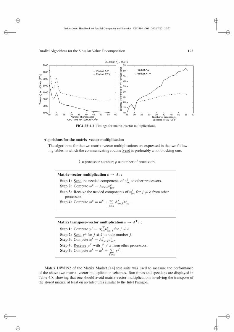
�
�
Erricos John: Handbook on Parallel Computing and Statistics DK2384 c004 2005/7/20 20:27�
�
�
�
�
�
Parallel Algorithms for the Singular Value Decomposition 153
15 20 25 30 35 40 45 50 55 601000
2000
3000
4000
5000
6000
7000
8000
− Product A.V −. Product AT.V
15 20 25 30 35 40 45 50 55 6010
15
20
25
30
35
40
45
50
55
Number of processorsSpeedup for AV / ATV
Spe
edup
(re
fere
nced
on
r=17
pro
cess
ors) − Product A.V
−. Product AT.V
Number of processorsCPU Time for 1000 AV / ATV
Tim
e (m
s) fo
r 10
00 A
V (
AT
V)
n = 8192, nz = 41,746
FIGURE 4.2 Timings for matrix–vector multiplications.
Algorithms for the matrix–vector multiplication
The algorithms for the two matrix–vector multiplications are expressed in the two follow-ing tables in which the communicating routine Send is preferably a nonblocking one.
k = processor number; p = number of processors.
Matrix–vector multiplication v → Av:
Step 1: Send the needed components of vkloc to other processors.
Step 2: Compute wk = Aloc,kvkloc.
Step 3: Receive the needed components of vjloc for j = k from other
processors.Step 4: Compute wk = wk + ∑
j =kA j
ext,kvjloc.
Matrix transpose–vector multiplication v → ATv :
Step 1: Compute y j = A jTextv
kloc, j for j = k.
Step 2: Send y j for j = k to node number j .Step 3: Compute wk = AT
loc,kvkloc.
Step 4: Receive y j ′ with j ′ = k from other processors.Step 5: Compute wk = wk + ∑
j ′ =ky j ′ .
Matrix DW8192 of the Matrix Market [14] test suite was used to measure the performanceof the above two matrix–vector multiplication schemes. Run times and speedups are displayed inTable 4.8, showing that one should avoid matrix-vector multiplications involving the transpose ofthe stored matrix, at least on architectures similar to the Intel Paragon.
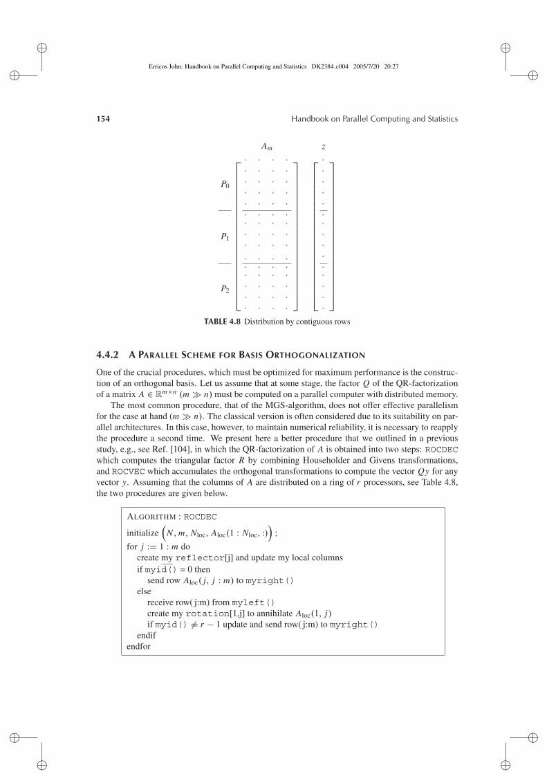
�
�
Erricos John: Handbook on Parallel Computing and Statistics DK2384 c004 2005/7/20 20:27�
�
�
�
�
�
154 Handbook on Parallel Computing and Statistics
P0
P1
P2
Am
⎡⎢⎢⎢⎢⎢⎢⎢⎢⎢⎢⎢⎢⎢⎢⎢⎢⎢⎢⎢⎢⎢⎣
· · · ·· · · ·· · · ·· · · ·· · · ·· · · ·· · · ·· · · ·· · · ·· · · ·· · · ·· · · ·· · · ·· · · ·· · · ·
⎤⎥⎥⎥⎥⎥⎥⎥⎥⎥⎥⎥⎥⎥⎥⎥⎥⎥⎥⎥⎥⎥⎦
z
⎡⎢⎢⎢⎢⎢⎢⎢⎢⎢⎢⎢⎢⎢⎢⎢⎢⎢⎢⎢⎢⎢⎣
···············
⎤⎥⎥⎥⎥⎥⎥⎥⎥⎥⎥⎥⎥⎥⎥⎥⎥⎥⎥⎥⎥⎥⎦
TABLE 4.8 Distribution by contiguous rows
4.4.2 A PARALLEL SCHEME FOR BASIS ORTHOGONALIZATION
One of the crucial procedures, which must be optimized for maximum performance is the construc-tion of an orthogonal basis. Let us assume that at some stage, the factor Q of the QR-factorizationof a matrix A ∈ R
m×n (m � n) must be computed on a parallel computer with distributed memory.The most common procedure, that of the MGS-algorithm, does not offer effective parallelism
for the case at hand (m � n). The classical version is often considered due to its suitability on par-allel architectures. In this case, however, to maintain numerical reliability, it is necessary to reapplythe procedure a second time. We present here a better procedure that we outlined in a previousstudy, e.g., see Ref. [104], in which the QR-factorization of A is obtained into two steps: ROCDECwhich computes the triangular factor R by combining Householder and Givens transformations,and ROCVEC which accumulates the orthogonal transformations to compute the vector Qy for anyvector y. Assuming that the columns of A are distributed on a ring of r processors, see Table 4.8,the two procedures are given below.
ALGORITHM : ROCDEC
initialize(
N , m, Nloc, Aloc(1 : Nloc, :))
;
for j := 1 : m docreate my reflector[j] and update my local columnsif myid() = 0 then
send row Aloc( j, j : m) to myright()else
receive row( j:m) from myleft()create my rotation[1,j] to annihilate Aloc(1, j)if myid() = r − 1 update and send row( j:m) to myright()
endifendfor
�
�
Erricos John: Handbook on Parallel Computing and Statistics DK2384 c004 2005/7/20 20:27�
�
�
�
�
�
Parallel Algorithms for the Singular Value Decomposition 155
At completion the factor Q is explicitly available but is shared in the same fashion that theoriginal matrix Am at the beginning. Hence, the product z = Qy is trivial.
ALGORITHM : ROCVEC
k := myid() ;zloc := 0 ;{ apply orthogonal transformations in reverse order }for j := m : 1 step −1 do
if (k = 0) thenreceive zloc( j) from myright()i := j ;
elseif (k = r − 1) then
apply my rotation[1, j] on [y( j), zloc(1)]send the updated y( j) to myleft()
elsereceive yj from myright()apply my rotation[1, j] on [y j, zloc(1)]send the updated yj to myleft()
endifi := 1 ;
endifapply my reflector[ j] on zloc(i : Nloc)
endfor
Data distribution. The factor R is sent to processor Pr−1. To compute the product z = Qy thevector y ∈ R
m must be at the beginning in processor Pr−1. The resulting vector z ∈ RN is split at
completion.
Parallelism. The application of Householder reflectors is a completely independent stage.However, to annihilate the remaining nonzero elements through Givens rotations, it is necessaryto transport a row portion along r processors. But as soon as that portion is passed througha processor, the latter applies its next reflector so that there is an overlapping of its computa-tions and the transfer of that row portion to the other processors. Since there will be a totalof m transfers of this sort during the whole factorization, communication overheads willbe masked if m � r . In summary, we expect a reasonable speedup when (n/r) � m andm � r .
Experiment. The following experiment illustrates the superior scalability of the scheme ROC(ROC=ROCDEC+ROCVEC) with respect to the MGS procedure. The goal is to compute Qy whereQ is the Q-factor in the QR-factorization of A. In Table 4.9, we give the running times (in seconds)of the two algorithms with a constant computing load per processor. The column length is n = 104rand the number of columns is m = 40. The algorithm ROC appears to be much more scalable thanMGS.
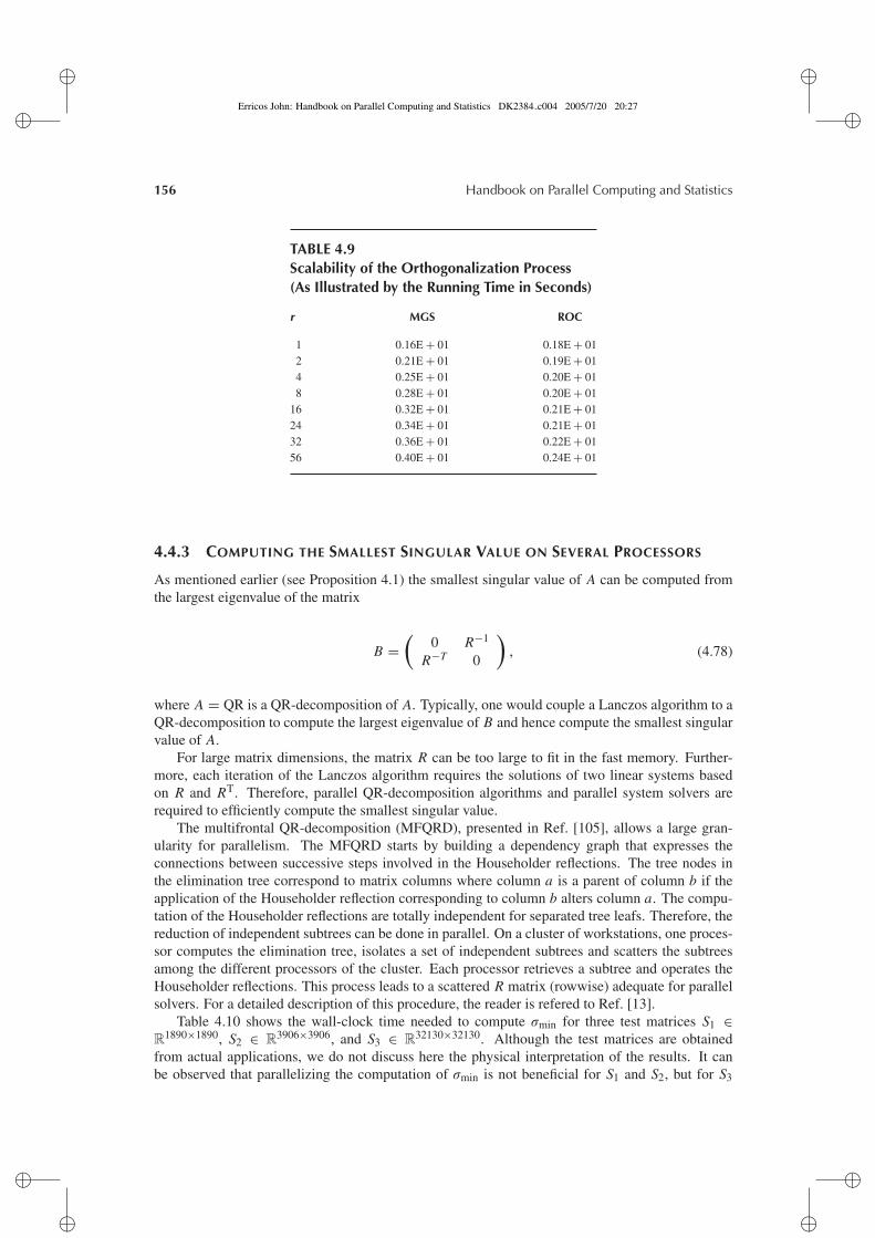
�
�
Erricos John: Handbook on Parallel Computing and Statistics DK2384 c004 2005/7/20 20:27�
�
�
�
�
�
156 Handbook on Parallel Computing and Statistics
TABLE 4.9Scalability of the Orthogonalization Process(As Illustrated by the Running Time in Seconds)
r MGS ROC
1 0.16E + 01 0.18E + 012 0.21E + 01 0.19E + 014 0.25E + 01 0.20E + 018 0.28E + 01 0.20E + 01
16 0.32E + 01 0.21E + 0124 0.34E + 01 0.21E + 0132 0.36E + 01 0.22E + 0156 0.40E + 01 0.24E + 01
4.4.3 COMPUTING THE SMALLEST SINGULAR VALUE ON SEVERAL PROCESSORS
As mentioned earlier (see Proposition 4.1) the smallest singular value of A can be computed fromthe largest eigenvalue of the matrix
B =(
0 R−1
R−T 0
), (4.78)
where A = QR is a QR-decomposition of A. Typically, one would couple a Lanczos algorithm to aQR-decomposition to compute the largest eigenvalue of B and hence compute the smallest singularvalue of A.
For large matrix dimensions, the matrix R can be too large to fit in the fast memory. Further-more, each iteration of the Lanczos algorithm requires the solutions of two linear systems basedon R and RT. Therefore, parallel QR-decomposition algorithms and parallel system solvers arerequired to efficiently compute the smallest singular value.
The multifrontal QR-decomposition (MFQRD), presented in Ref. [105], allows a large gran-ularity for parallelism. The MFQRD starts by building a dependency graph that expresses theconnections between successive steps involved in the Householder reflections. The tree nodes inthe elimination tree correspond to matrix columns where column a is a parent of column b if theapplication of the Householder reflection corresponding to column b alters column a. The compu-tation of the Householder reflections are totally independent for separated tree leafs. Therefore, thereduction of independent subtrees can be done in parallel. On a cluster of workstations, one proces-sor computes the elimination tree, isolates a set of independent subtrees and scatters the subtreesamong the different processors of the cluster. Each processor retrieves a subtree and operates theHouseholder reflections. This process leads to a scattered R matrix (rowwise) adequate for parallelsolvers. For a detailed description of this procedure, the reader is refered to Ref. [13].
Table 4.10 shows the wall-clock time needed to compute σmin for three test matrices S1 ∈R
1890×1890, S2 ∈ R3906×3906, and S3 ∈ R
32130×32130. Although the test matrices are obtainedfrom actual applications, we do not discuss here the physical interpretation of the results. It canbe observed that parallelizing the computation of σmin is not beneficial for S1 and S2, but for S3
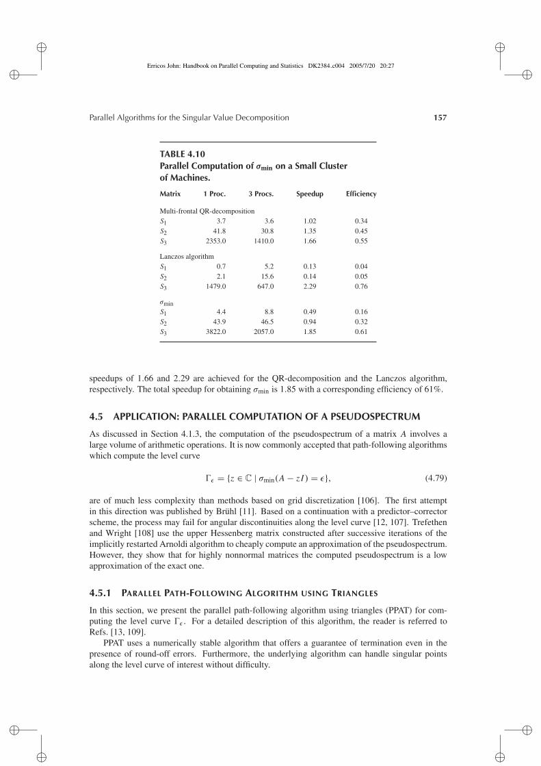
�
�
Erricos John: Handbook on Parallel Computing and Statistics DK2384 c004 2005/7/20 20:27�
�
�
�
�
�
Parallel Algorithms for the Singular Value Decomposition 157
TABLE 4.10Parallel Computation of σmin on a Small Clusterof Machines.
Matrix 1 Proc. 3 Procs. Speedup Efficiency
Multi-frontal QR-decompositionS1 3.7 3.6 1.02 0.34S2 41.8 30.8 1.35 0.45S3 2353.0 1410.0 1.66 0.55
Lanczos algorithmS1 0.7 5.2 0.13 0.04S2 2.1 15.6 0.14 0.05S3 1479.0 647.0 2.29 0.76
σminS1 4.4 8.8 0.49 0.16S2 43.9 46.5 0.94 0.32S3 3822.0 2057.0 1.85 0.61
speedups of 1.66 and 2.29 are achieved for the QR-decomposition and the Lanczos algorithm,respectively. The total speedup for obtaining σmin is 1.85 with a corresponding efficiency of 61%.
4.5 APPLICATION: PARALLEL COMPUTATION OF A PSEUDOSPECTRUM
As discussed in Section 4.1.3, the computation of the pseudospectrum of a matrix A involves alarge volume of arithmetic operations. It is now commonly accepted that path-following algorithmswhich compute the level curve
�ε = {z ∈ C | σmin(A − z I ) = ε}, (4.79)
are of much less complexity than methods based on grid discretization [106]. The first attemptin this direction was published by Bruhl [11]. Based on a continuation with a predictor–correctorscheme, the process may fail for angular discontinuities along the level curve [12, 107]. Trefethenand Wright [108] use the upper Hessenberg matrix constructed after successive iterations of theimplicitly restarted Arnoldi algorithm to cheaply compute an approximation of the pseudospectrum.However, they show that for highly nonnormal matrices the computed pseudospectrum is a lowapproximation of the exact one.
4.5.1 PARALLEL PATH-FOLLOWING ALGORITHM USING TRIANGLES
In this section, we present the parallel path-following algorithm using triangles (PPAT) for com-puting the level curve �ε . For a detailed description of this algorithm, the reader is referred toRefs. [13, 109].
PPAT uses a numerically stable algorithm that offers a guarantee of termination even in thepresence of round-off errors. Furthermore, the underlying algorithm can handle singular pointsalong the level curve of interest without difficulty.
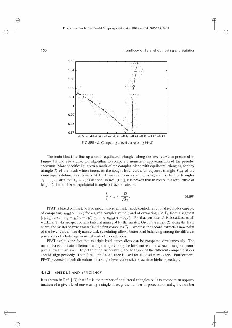
�
�
Erricos John: Handbook on Parallel Computing and Statistics DK2384 c004 2005/7/20 20:27�
�
�
�
�
�
158 Handbook on Parallel Computing and Statistics
−0.5 −0.49 −0.48 −0.47 −0.46 −0.45 −0.44 −0.43 −0.42 −0.410.97
0.98
0.99
1
1.01
1.02
1.03
1.04
1.05
FIGURE 4.3 Computing a level curve using PPAT.
The main idea is to line up a set of equilateral triangles along the level curve as presented inFigure 4.3 and use a bisection algorithm to compute a numerical approximation of the pseudo-spectrum. More specifically, given a mesh of the complex plane with equilateral triangles, for anytriangle Ti of the mesh which intersects the sought-level curve, an adjacent triangle Ti+1 of thesame type is defined as successor of Ti . Therefore, from a starting triangle T0, a chain of trianglesT1, . . . , Tn such that Tn = T0 is defined. In Ref. [109], it is proven that to compute a level curve oflength l, the number of equilateral triangles of size τ satisfies
l
τ≤ n ≤ 10l√
3τ. (4.80)
PPAT is based on master-slave model where a master node controls a set of slave nodes capableof computing σmin(A − z I ) for a given complex value z and of extracting z ∈ �ε from a segment[zl, zg], assuming σmin(A − zl I ) ≤ ε < σmin(A − zg I ). For that purpose, A is broadcast to allworkers. Tasks are queued in a task list managed by the master. Given a triangle Ti along the levelcurve, the master spawns two tasks; the first computes Ti+1 whereas the second extracts a new pointof the level curve. The dynamic task scheduling allows better load balancing among the differentprocessors of a heterogeneous network of workstations.
PPAT exploits the fact that multiple level curve slices can be computed simultaneously. Themain idea is to locate different starting triangles along the level curve and use each triangle to com-pute a level curve slice. To get through successfully, the triangles of the different computed slicesshould align perfectly. Therefore, a prefixed lattice is used for all level curve slices. Furthermore,PPAT proceeds in both directions on a single level curve slice to achieve higher speedups.
4.5.2 SPEEDUP AND EFFICIENCY
It is shown in Ref. [13] that if n is the number of equilateral triangles built to compute an approx-imation of a given level curve using a single slice, p the number of processors, and q the number
�
�
Erricos John: Handbook on Parallel Computing and Statistics DK2384 c004 2005/7/20 20:27�
�
�
�
�
�
Parallel Algorithms for the Singular Value Decomposition 159
of evaluations of σmin for each bisection process, then the speedup is given by
Sp =
⎧⎪⎪⎪⎨⎪⎪⎪⎩
2n(q + 1)
n + 2qif p ≥ 2q + 2,
2np(q + 1)
p2 − 2p + 2n(q + 1)if p < 2q + 2.
(4.81)
For large values of n, the speedup and efficiency can be expressed as
Sp = min(p, 2q + 2) + O(1/n),
and
E p = min
(1,
2q + 2
p
)+ O(1/n).
The upper bound of the speedup is given by Smax = 2q + 2. This limit is theoretically achievedwhenever p ≥ 2q + 2.
4.5.3 TEST PROBLEMS
Three test matrices were selected from the Matrix Market suite [14]. Table 4.11 summarizes theircharacteristics (N z is the number of nonzero entries and tσmin is the average computation time forσmin(A − z I )). The application uses up to 20 workers, where the master process shares the samephysical processor as the first worker. The underlying hardware is a low-cost general purposenetwork of personal computers (Pentium III, 600 MHz, 128 MB RAM).
Figure 4.4 displays speedups and efficiencies for computing 100 points on a given level curvewith PPAT. The best performance was observed for matrix Dw8192 which is the largest of the set; aspeedup of 10.85 using 12 processors which corresponds to a 90% efficiency. The lowest efficiencyobtained was 63% for Olm1000 on 13 processors. In a more realistic approach, we have usedthe 70 processors of the PARASKI cluster at IRISA to compute, in 41 s, the level curve ε = 0.05of Olm1000 split into 15 slices. A single processor required 4020 s to compute the same levelcurve. The corresponding speedup is 98 with an efficiency greater than 1, indicating higher datalocality realized for each processor. This result indicates the favorable scalability of PPAT becausePARASKI is a heterogeneous cluster of processors ranging from PII to PIV; the sequential time ismeasured on a randomly selected PIII of the cluster.
TABLE 4.11Test Matrices from the Non-Hermitian Eigenvalue problem(NEP) Collection
Matrix Order Nz ||A||F tσmin (s)
Olm1000 1,000 3,996 1.3 × 10⁶ 0.27Rdb3200L 3,200 18,880 2.8 × 10³ 15.14Dw8192 8,192 41,746 1.6 × 10³ 114.36
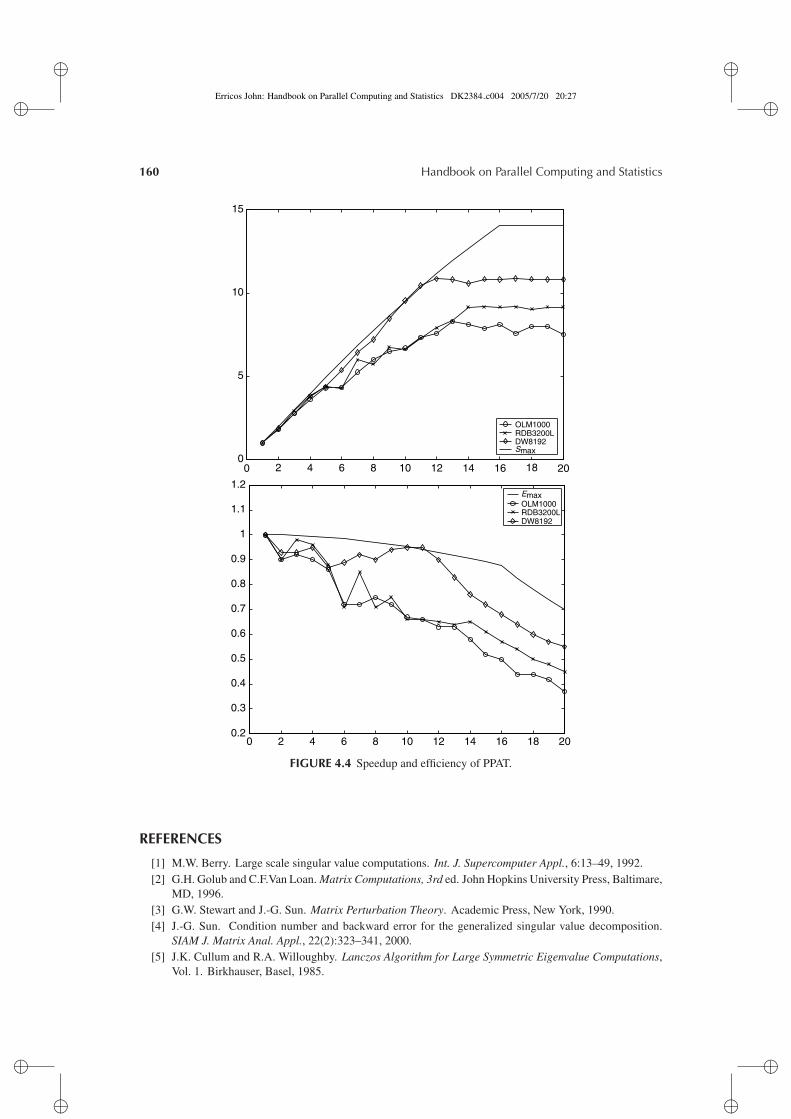
�
�
Erricos John: Handbook on Parallel Computing and Statistics DK2384 c004 2005/7/20 20:27�
�
�
�
�
�
160 Handbook on Parallel Computing and Statistics
0 2 4 6 8 10 12 14 16 18 200
5
10
15
OLM1000RDB3200LDW8192Smax
0 2 4 6 8 10 12 14 16 18 200.2
0.3
0.4
0.5
0.6
0.7
0.8
0.9
1
1.1
1.2EmaxOLM1000RDB3200LDW8192
FIGURE 4.4 Speedup and efficiency of PPAT.
REFERENCES
[1] M.W. Berry. Large scale singular value computations. Int. J. Supercomputer Appl., 6:13–49, 1992.[2] G.H. Golub and C.F.Van Loan. Matrix Computations, 3rd ed. John Hopkins University Press, Baltimare,
MD, 1996.[3] G.W. Stewart and J.-G. Sun. Matrix Perturbation Theory. Academic Press, New York, 1990.[4] J.-G. Sun. Condition number and backward error for the generalized singular value decomposition.
SIAM J. Matrix Anal. Appl., 22(2):323–341, 2000.[5] J.K. Cullum and R.A. Willoughby. Lanczos Algorithm for Large Symmetric Eigenvalue Computations,
Vol. 1. Birkhauser, Basel, 1985.
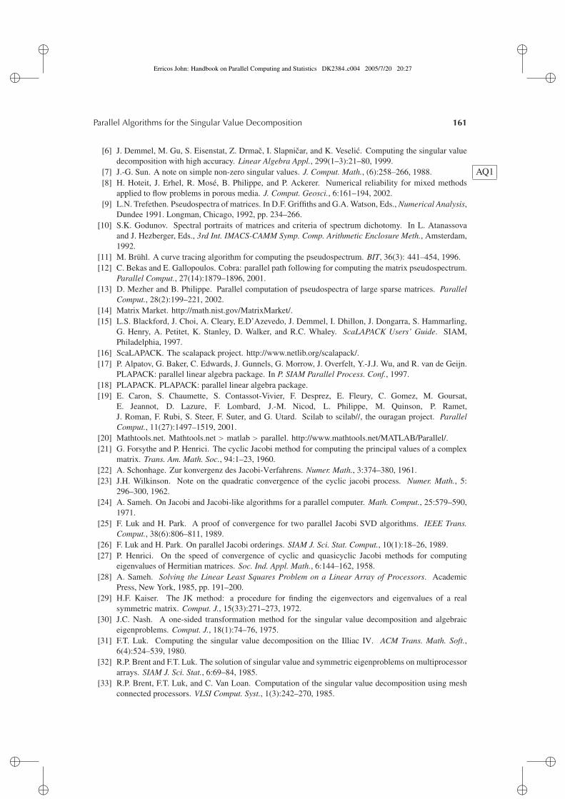
�
�
Erricos John: Handbook on Parallel Computing and Statistics DK2384 c004 2005/7/20 20:27�
�
�
�
�
�
Parallel Algorithms for the Singular Value Decomposition 161
[6] J. Demmel, M. Gu, S. Eisenstat, Z. Drmac, I. Slapnicar, and K. Veselic. Computing the singular valuedecomposition with high accuracy. Linear Algebra Appl., 299(1–3):21–80, 1999.
[7] J.-G. Sun. A note on simple non-zero singular values. J. Comput. Math., (6):258–266, 1988. AQ1[8] H. Hoteit, J. Erhel, R. Mose, B. Philippe, and P. Ackerer. Numerical reliability for mixed methods
applied to flow problems in porous media. J. Comput. Geosci., 6:161–194, 2002.[9] L.N. Trefethen. Pseudospectra of matrices. In D.F. Griffiths and G.A. Watson, Eds., Numerical Analysis,
Dundee 1991. Longman, Chicago, 1992, pp. 234–266.[10] S.K. Godunov. Spectral portraits of matrices and criteria of spectrum dichotomy. In L. Atanassova
and J. Hezberger, Eds., 3rd Int. IMACS-CAMM Symp. Comp. Arithmetic Enclosure Meth., Amsterdam,1992.
[11] M. Bruhl. A curve tracing algorithm for computing the pseudospectrum. BIT, 36(3): 441–454, 1996.[12] C. Bekas and E. Gallopoulos. Cobra: parallel path following for computing the matrix pseudospectrum.
Parallel Comput., 27(14):1879–1896, 2001.[13] D. Mezher and B. Philippe. Parallel computation of pseudospectra of large sparse matrices. Parallel
Comput., 28(2):199–221, 2002.[14] Matrix Market. http://math.nist.gov/MatrixMarket/.[15] L.S. Blackford, J. Choi, A. Cleary, E.D’Azevedo, J. Demmel, I. Dhillon, J. Dongarra, S. Hammarling,
G. Henry, A. Petitet, K. Stanley, D. Walker, and R.C. Whaley. ScaLAPACK Users’ Guide. SIAM,Philadelphia, 1997.
[16] ScaLAPACK. The scalapack project. http://www.netlib.org/scalapack/.[17] P. Alpatov, G. Baker, C. Edwards, J. Gunnels, G. Morrow, J. Overfelt, Y.-J.J. Wu, and R. van de Geijn.
PLAPACK: parallel linear algebra package. In P. SIAM Parallel Process. Conf., 1997.[18] PLAPACK. PLAPACK: parallel linear algebra package.[19] E. Caron, S. Chaumette, S. Contassot-Vivier, F. Desprez, E. Fleury, C. Gomez, M. Goursat,
E. Jeannot, D. Lazure, F. Lombard, J.-M. Nicod, L. Philippe, M. Quinson, P. Ramet,J. Roman, F. Rubi, S. Steer, F. Suter, and G. Utard. Scilab to scilab//, the ouragan project. ParallelComput., 11(27):1497–1519, 2001.
[20] Mathtools.net. Mathtools.net > matlab > parallel. http://www.mathtools.net/MATLAB/Parallel/.[21] G. Forsythe and P. Henrici. The cyclic Jacobi method for computing the principal values of a complex
matrix. Trans. Am. Math. Soc., 94:1–23, 1960.[22] A. Schonhage. Zur konvergenz des Jacobi-Verfahrens. Numer. Math., 3:374–380, 1961.[23] J.H. Wilkinson. Note on the quadratic convergence of the cyclic jacobi process. Numer. Math., 5:
296–300, 1962.[24] A. Sameh. On Jacobi and Jacobi-like algorithms for a parallel computer. Math. Comput., 25:579–590,
1971.[25] F. Luk and H. Park. A proof of convergence for two parallel Jacobi SVD algorithms. IEEE Trans.
Comput., 38(6):806–811, 1989.[26] F. Luk and H. Park. On parallel Jacobi orderings. SIAM J. Sci. Stat. Comput., 10(1):18–26, 1989.[27] P. Henrici. On the speed of convergence of cyclic and quasicyclic Jacobi methods for computing
eigenvalues of Hermitian matrices. Soc. Ind. Appl. Math., 6:144–162, 1958.[28] A. Sameh. Solving the Linear Least Squares Problem on a Linear Array of Processors. Academic
Press, New York, 1985, pp. 191–200.[29] H.F. Kaiser. The JK method: a procedure for finding the eigenvectors and eigenvalues of a real
symmetric matrix. Comput. J., 15(33):271–273, 1972.[30] J.C. Nash. A one-sided transformation method for the singular value decomposition and algebraic
eigenproblems. Comput. J., 18(1):74–76, 1975.[31] F.T. Luk. Computing the singular value decomposition on the Illiac IV. ACM Trans. Math. Soft.,
6(4):524–539, 1980.[32] R.P. Brent and F.T. Luk. The solution of singular value and symmetric eigenproblems on multiprocessor
arrays. SIAM J. Sci. Stat., 6:69–84, 1985.[33] R.P. Brent, F.T. Luk, and C. Van Loan. Computation of the singular value decomposition using mesh
connected processors. VLSI Comput. Syst., 1(3):242–270, 1985.
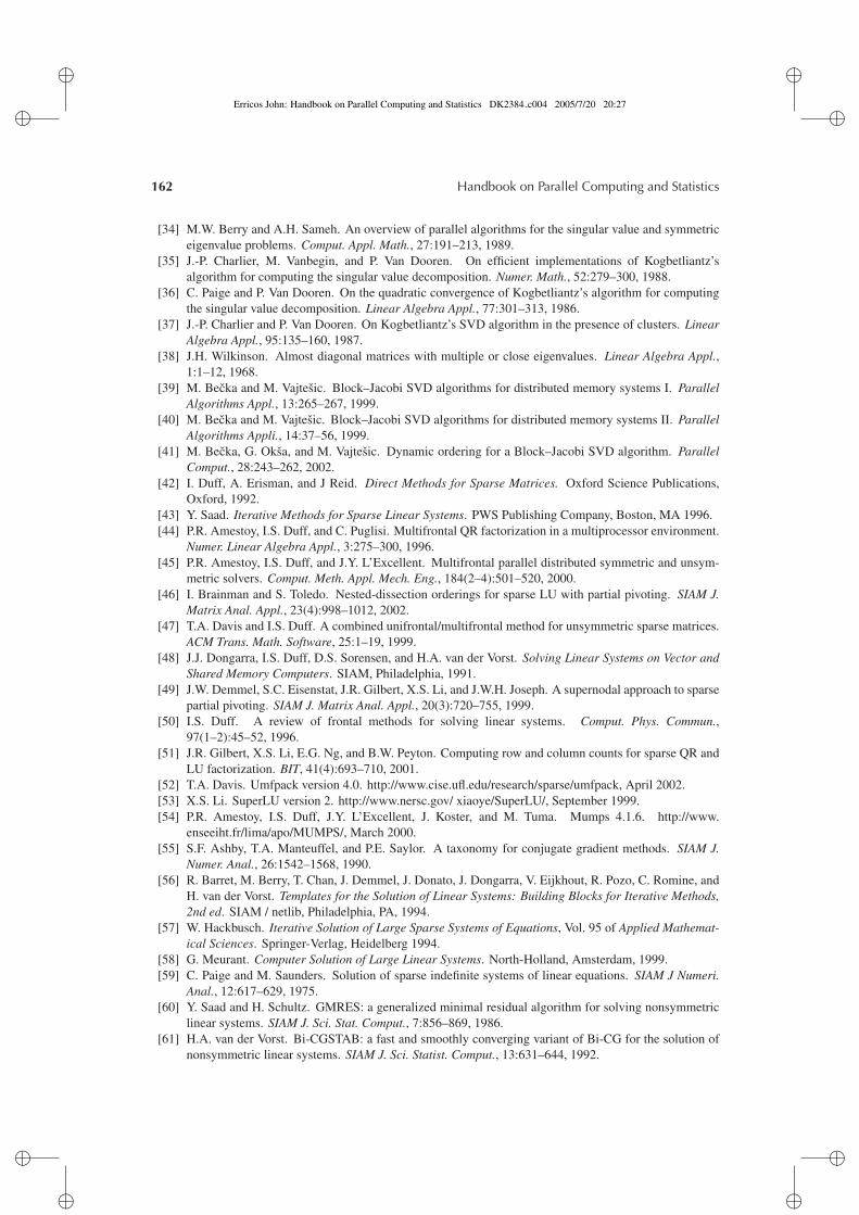
�
�
Erricos John: Handbook on Parallel Computing and Statistics DK2384 c004 2005/7/20 20:27�
�
�
�
�
�
162 Handbook on Parallel Computing and Statistics
[34] M.W. Berry and A.H. Sameh. An overview of parallel algorithms for the singular value and symmetriceigenvalue problems. Comput. Appl. Math., 27:191–213, 1989.
[35] J.-P. Charlier, M. Vanbegin, and P. Van Dooren. On efficient implementations of Kogbetliantz’salgorithm for computing the singular value decomposition. Numer. Math., 52:279–300, 1988.
[36] C. Paige and P. Van Dooren. On the quadratic convergence of Kogbetliantz’s algorithm for computingthe singular value decomposition. Linear Algebra Appl., 77:301–313, 1986.
[37] J.-P. Charlier and P. Van Dooren. On Kogbetliantz’s SVD algorithm in the presence of clusters. LinearAlgebra Appl., 95:135–160, 1987.
[38] J.H. Wilkinson. Almost diagonal matrices with multiple or close eigenvalues. Linear Algebra Appl.,1:1–12, 1968.
[39] M. Becka and M. Vajtesic. Block–Jacobi SVD algorithms for distributed memory systems I. ParallelAlgorithms Appl., 13:265–267, 1999.
[40] M. Becka and M. Vajtesic. Block–Jacobi SVD algorithms for distributed memory systems II. ParallelAlgorithms Appli., 14:37–56, 1999.
[41] M. Becka, G. Oksa, and M. Vajtesic. Dynamic ordering for a Block–Jacobi SVD algorithm. ParallelComput., 28:243–262, 2002.
[42] I. Duff, A. Erisman, and J Reid. Direct Methods for Sparse Matrices. Oxford Science Publications,Oxford, 1992.
[43] Y. Saad. Iterative Methods for Sparse Linear Systems. PWS Publishing Company, Boston, MA 1996.[44] P.R. Amestoy, I.S. Duff, and C. Puglisi. Multifrontal QR factorization in a multiprocessor environment.
Numer. Linear Algebra Appl., 3:275–300, 1996.[45] P.R. Amestoy, I.S. Duff, and J.Y. L’Excellent. Multifrontal parallel distributed symmetric and unsym-
metric solvers. Comput. Meth. Appl. Mech. Eng., 184(2–4):501–520, 2000.[46] I. Brainman and S. Toledo. Nested-dissection orderings for sparse LU with partial pivoting. SIAM J.
Matrix Anal. Appl., 23(4):998–1012, 2002.[47] T.A. Davis and I.S. Duff. A combined unifrontal/multifrontal method for unsymmetric sparse matrices.
ACM Trans. Math. Software, 25:1–19, 1999.[48] J.J. Dongarra, I.S. Duff, D.S. Sorensen, and H.A. van der Vorst. Solving Linear Systems on Vector and
Shared Memory Computers. SIAM, Philadelphia, 1991.[49] J.W. Demmel, S.C. Eisenstat, J.R. Gilbert, X.S. Li, and J.W.H. Joseph. A supernodal approach to sparse
partial pivoting. SIAM J. Matrix Anal. Appl., 20(3):720–755, 1999.[50] I.S. Duff. A review of frontal methods for solving linear systems. Comput. Phys. Commun.,
97(1–2):45–52, 1996.[51] J.R. Gilbert, X.S. Li, E.G. Ng, and B.W. Peyton. Computing row and column counts for sparse QR and
LU factorization. BIT, 41(4):693–710, 2001.[52] T.A. Davis. Umfpack version 4.0. http://www.cise.ufl.edu/research/sparse/umfpack, April 2002.[53] X.S. Li. SuperLU version 2. http://www.nersc.gov/ xiaoye/SuperLU/, September 1999.[54] P.R. Amestoy, I.S. Duff, J.Y. L’Excellent, J. Koster, and M. Tuma. Mumps 4.1.6. http://www.
enseeiht.fr/lima/apo/MUMPS/, March 2000.[55] S.F. Ashby, T.A. Manteuffel, and P.E. Saylor. A taxonomy for conjugate gradient methods. SIAM J.
Numer. Anal., 26:1542–1568, 1990.[56] R. Barret, M. Berry, T. Chan, J. Demmel, J. Donato, J. Dongarra, V. Eijkhout, R. Pozo, C. Romine, and
H. van der Vorst. Templates for the Solution of Linear Systems: Building Blocks for Iterative Methods,2nd ed. SIAM / netlib, Philadelphia, PA, 1994.
[57] W. Hackbusch. Iterative Solution of Large Sparse Systems of Equations, Vol. 95 of Applied Mathemat-ical Sciences. Springer-Verlag, Heidelberg 1994.
[58] G. Meurant. Computer Solution of Large Linear Systems. North-Holland, Amsterdam, 1999.[59] C. Paige and M. Saunders. Solution of sparse indefinite systems of linear equations. SIAM J Numeri.
Anal., 12:617–629, 1975.[60] Y. Saad and H. Schultz. GMRES: a generalized minimal residual algorithm for solving nonsymmetric
linear systems. SIAM J. Sci. Stat. Comput., 7:856–869, 1986.[61] H.A. van der Vorst. Bi-CGSTAB: a fast and smoothly converging variant of Bi-CG for the solution of
nonsymmetric linear systems. SIAM J. Sci. Statist. Comput., 13:631–644, 1992.
�
�
Erricos John: Handbook on Parallel Computing and Statistics DK2384 c004 2005/7/20 20:27�
�
�
�
�
�
Parallel Algorithms for the Singular Value Decomposition 163
[62] R. Freund and N. Nachtigal. QMR: a quasi-minimal residual method for non-Hermitian linear systems.Numer. Math., 60:315–339, 1991.
[63] R. Freund. A transpose-free quasi-minimal residual algorithm for non-Hermitian linear systems. SIAMJ. Sci. comput., 14:470–482, 1993.
[64] G.H. Golub and W. Kahan. Calculating the singular values and pseudo-inverse of a matrix. SIAM J.Numer. Anal., 2(3):205–224, 1965.
[65] G.H. Golub and C. Reinsch. Singular Value Decomposition and Least Squares Solutions. Springer-Verlag, Heidelberg, 1971.
[66] M.R. Hestens. Inversion of matrices by biorthogonalization and related results. Soc. Ind. Appl. Math.,6:51–90, 1958.
[67] B.N. Parlett. The Symmetric Eigenvalue Problem. Prentice Hall, New York, 1980.[68] F.L. Bauer. Das verfahred der treppeniteration und verwandte verfahren zur losung algebraischer eigen-
wertprobleme. ZAMP, 8:214–235, 1957.[69] H. Rutishauser. Simultaneous iteration method for symmetric matrices. Numer. Math., 16:205–223,
1970.[70] K. Gallivan, W. Jalby, and U. Meier. The use of BLAS3 in linear algebra on a parallel processor with a
hierarchical memory. SIAM J. Sci. Stat. Comput., 18(6):1079–1084, 1987.[71] H. Rutishauser. Computational aspects of F.L. Bauer’s simultaneous iteration method. Numer. Math.,
13:4–13, 1969.[72] B. Smith, J. Boyce, J. Dongarra, B. Garbow, Y. Ikebe, V. Klema, and C. Moler. Matrix Eigensystem
Routines — EISPACK Guide, 2nd ed. Springer-Verlag, Heidelberg, 1976.[73] J. Dongarra and D. Sorensen. A fast algorithm for the symmetric eigenvalue problem. SIAM J. Sci. Stat.
Comput., 8(2):s139–s154, 1987.[74] C.C. Paige. Error analysis of the Lanczos algorithms for tridiagonalizing a symmetric matrix. Inst.
Math. Appl., 18:341–349, 1976.[75] J. Grcar. Analysis of the Lanczos Algorithm and of the Approximation Problem in Richardson’s
Method, Ph.D. Thesis. Technical report, The University of Illinois, Chicago, 1981.[76] B.N. Parlett and D.S. Scott. The Lanczos algorithm with selective reorthogonalization. Math. Comput.,
33:217–238, 1979.[77] H. Simon. Analysis of the symmetric Lanczos algorithm with reorthogonalization methods. Linear
Algebra Appl., 61:101–131, 1984.[78] S. Lo, B. Philippe, and A.H. Sameh. A multiprocessor algorithm for the symmetric tridiagonal
eigenvalue problem. SIAM J. Sci. Stat. Comput., 8(2):s155–s165, 1987.[79] G.H. Golub and C. Van Loan. Matrix Computations, 2nd ed. Johns Hopkins University Press,
Battimore, MD, 1989.[80] R.R. Underwood. An Iterative Block Lanczos Method for the Solution of Large Sparse Symmetric
Eigenproblems, Ph.D. thesis. Technical report, Stanford University, Stanford, 1975.[81] G.H. Golub and R.R. Underwood. The Block Lanczos Method for Computing Eigenvalues, Academic
Press, New York, 1977, pp. 361–377.[82] G.H. Golub, F.T. Luk, and M.L. Overton. A block Lanczos method for computing the singular values
and corresponding singular vectors of a matrix. ACM Trans. Math. Software, 7(2):149–169, 1981.[83] J. Dongarra, J. Du Croz, S. Hammarling, and R. Hanson. An extended set of FORTRAN basic linear
algebra subprograms. ACM Trans. Math. Software, 14(1):1–17, 1988.[84] W. Jalby and B. Philippe. Stability analysis and improvement of the block Gram–Schmidt algorithm.
SIAM J. Sci. Stat. Comput., 12(5):1058–1073, 1991.[85] A.H. Sameh and J.A. Wisniewski. A trace minimization algorithm for the generalized eigenvalue
problem. SIAM J. Numer. Anal., 19(6):1243–1259, 1982.[86] J.H. Wilkinson. The Algebraic Eigenvalue Problem. Clarendon Press, Oxford, 1965.[87] M.W. Berry, B. Parlett, and A.H. Sameh. Computing extremal singular triplets of sparse matrices on a
shared-memory multiprocessor. Int. J. High Speed Comput., 2:239–275, 1994.[88] D.G. Luenberger. Introduction to Linear and Nonlinear Programming. Addison-Wesley, Reading,
Massachusetts, 1973.
�
�
Erricos John: Handbook on Parallel Computing and Statistics DK2384 c004 2005/7/20 20:27�
�
�
�
�
�
164 Handbook on Parallel Computing and Statistics
[89] J.H. Wilkinson. Inverse Iteration in Theory and in Practice. Academic Press, New York, 1972.[90] E. Kokiopoulou, C. Bekas, and E. Gallopoulos. Computing Smallest Singular Triplets with Implic-
itly Restarted Lanczos Bidiagonalization. Technical report, Computer Eng. & Informatics Dept.,HPCLAB-TR-17-02-03. Appl. Numer. Math., 2003, to appear.AQ2
[91] J.O. Aasen. On the reduction of a symmetric matrix to tridiagonal form. BIT, 11:233–242, 1971.[92] J.R. Bunch and L. Kaufman. Some stable methods for calculating inertia and solving symmetric linear
systems. Math. Comput., 31:162–179, 1977.[93] B.N. Parlett and J.K. Reid. On the solution of a system of linear equations whose system is symmetric
but not definite. BIT, 10:386–397, 1970.[94] C.C. Paige and M.A. Saunders. Solution of sparse indefinite systems of linear equations. SIAM J.
Numer. Anal., 12(4):617–629, 1975.[95] E.R. Davidson. The iterative calculation of a few of the lowest eigenvalues and corresponding
eigenvectors of large real-symmetric matrices. Comput. Phys., 17:87–94, 1975.[96] R.B. Morgan and D.S. Scott. Generalizations of Davidson’s method for computing eigenvalues of sparse
symmetric matrices. SIAM J. Sci. Stat. Comput., 7:817–825, 1986.[97] M. Crouzeix, B. Philippe, and M. Sadkane. The Davidson method. SIAM J. Sci. Stat. Comput., 15:1:
62–76, 1994.[98] G.L.G. Sleipen and H.A. van der Vorst. A Jacobi–Davidson iteration method for linear eigenvalue
problems. SIAM J. Matrix Anal. Appl., 17(2):401–425, 1996. Also SIGEST in SIAM Rev. 42(2):267–293.
[99] A. Sameh and Z. Tong. The trace minimization method for the symmetric generalized eigenvalueproblem. J. Comput. Appl. Math., 123:155–175, 2000.
[100] V. Simoncini and L. Elden. Inexact Rayleigh quotient-type methods for eigenvalue computations. BIT,42(1):159–182, 2002.
[101] B. Philippe and M. Sadkane. Computation of the fundamental singular subspace of a large matrix.Linear Algebra Appl., 257:77–104, 1997.
[102] M.E. Hochstenbach. A Jacobi–Davidson type SVD method. SIAM J. Sci. Comput., 23(2):606–628,2001.
[103] V. Heuveline, B. Philippe, and M. Sadkane. Parallel computation of spectral portrait of large matricesby Davidson type methods. Numer. Algorithms, 16(1):55–75, 1997.
[104] R. Sidje and B. Philippe. Parallel Krylov subspace basis computation. In J. Tankoano, Ed., CARI’94Proc., Ouagadougou. INRIA — ORSTOM, ORSTOM Editions, Paris, 1994, pp. 421–440.
[105] P.R. Amestoy, I.S. Duff, and C. Puglisi. Multifrontal QR factorization in a multiprocessor environment.Numer. Linear Algebra Appl., 3:275–300, 1996.
[106] L.N. Trefethen. Computation of pseudospectra. Acta Numer., 247–295, 1999.AQ3[107] S.H. Lui. Computation of pseudospectra by continuation. SIAM J. Sci. Comput., 28(2): 565–573, 1997.[108] L.N. Trefethen and T. Wright. Large-scale Computation of Pseudospectra using ARPACK and Eigs.
Technical report, Oxford University Computing Laboratory, Oxford, June 2000.[109] D. Mezher and B. Philippe. PAT — a reliable path-following algorithm. Numer. Algorithms, 29:
131–152, 2002.
AUTHOR QUERIES
AQ1 Please provide vol. numberAQ2 Please updateAQ3 Please provide Vol. number