singular value decomposition and its application to

J. Inverse Ill-Posed Probl., Ahead of PrintDOI 10.1515/JIIP.2011.047 © de Gruyter 2011

Singular value decompositionand its application to numerical inversion for

ray transforms in 2D vector tomography

Evgeny Y. Derevtsov, Anton V. Efimov, Alfred K. Louis andThomas Schuster

Abstract. The operators of longitudinal and transverse ray transforms acting on vectorfields on the unit disc are considered in the paper. The goal is to construct SVD-decompo-sitions of the operators and invert them approximately by means of truncated decomposi-tion for the parallel scheme of data acquisition. The orthogonal bases in the initial spacesand the image spaces are constructed using harmonic, Jacobi and Gegenbauer polynomi-als. Based on the obtained decompositions inversion formulas are derived and the polyno-mial approximations for the inverse operators are obtained. Numerical tests for data setswith different noise levels of smooth and discontinuous fields show the validity of the ap-proach for the reconstruction of solenoidal or potential parts of vector fields from their raytransforms.

Keywords. Vector tomography, vector field, Radon transform, ray transform, singularvalue decomposition, orthogonal polynomials.

2010 Mathematics Subject Classification. 33C45, 42C05, 65R10, 65R32.

1 Introduction

The development both of mathematical approaches and of systems of data mea-surements and processing induced new mathematical models in tomography suchas thermotomography, diffusion tomography, vector and tensor tomography. Themodels appear due to the necessity of the reconstruction of properties of mediawith different degree of complication. Thus the tomography of vector fields arisesfor the description of vector characteristics of currents of fluids, vectors of electro-magnetic fields inside the conductor in inhomogeneous media, and many others.

We consider here a method of solving the vector tomography problem in a planein the case of parallel scheme of observation. As the problem of scalar tomography

The work has been supported by German Science Foundation (Deutsche Forschungsgemeinschaft,DFG) under grants LO310/11-1, SCHU 1978/5-1, Mathematical Department of RAS under grant1.3.8, RFBR under grant 11-07-00447, and SB RAS (Common Multi-discipline project SB and UrBRAS No 2009-14).

AUTHOR’S COPY | AUTORENEXEMPLAR


2 E. Y. Derevtsov, A. V. Efimov, A. K. Louis and T. Schuster

consists in the inversion of the Radon transform for a function, the vector tomo-graphy problem is the problem of inversion of ray transform operators applying tovector fields. In other words, one has to solve operator equations Af D g of thefirst kind. Here A is a linear, bounded operator, and coincides with one of the raytransform operators. There are longitudinal or transverse ray transforms. In the op-erator equation g is a known right hand-side (data of tomographic measurements),and f is an unknown vector field to be determined.

The method of singular value decomposition (SVD) is well known and oftenused for inversion of compact linear operators. The idea of the approach consistsin representing the operator in a form of series of singular numbers and basicelements in the image space. Then the inverse operator is a similar series with thereciprocal of the singular numbers and pre-images of the bases elements. SVD-de-composition for the operator of Radon transform acting on functions given in Rn

is well known ([2,3,10,11,17,19]). The SVD-decomposition of the ray transformin Rn, acting on functions, is constructed in [16]. In 2D the SVD-decompositionwas used to analyze the ill-posedness of the limited angle problem in [12], and forthe construction of inversion formulas for sparsely sampled data in [15]. In the 2D-case the SVD-decomposition for the operator of longitudinal ray transform, actingon symmetric tensor fields and reconstructing its solenoidal part, is known for fan-beam scheme of observation [8]. The polynomial bases for different subspaces ofvector fields given in the ball of R3 are constructed in [5]. In [20,21] reconstructionkernels for the longitudinal ray transform have been computed by means of theSVD of the 2D-Radon transform.

Here we reformulate the SVD-decomposition for the Radon operator, acting onfunctions given on the unit disk, in a form useful for the construction of SVD forthe operators of ray transform acting on vector fields.

For constructing the SVD-decompositions in the vector case we exploit the factthat every solenoidal v or potential u vector field in the plane can be defined by afunction (potential) according to

v D r? ;

for the solenoidal field, andu D r';

for potential field. Similarly to the scalar case we construct the potentials usingclassical polynomials. The constructed potentials form a non-orthogonal systemfor the potentials, but the arising solenoidal or potential vector fields are orthogonalin L2.S1.B//.

The algorithm for numerical inversion of the operators of longitudinal and trans-verse ray transforms is based on the constructed SVD-decompositions for the men-



SVD of ray transforms in 2D vector tomography 3

tioned operators. Numerical simulations show the validity of the approach leadingto good results of vector field reconstruction.

2 Preliminary definitions, objects and results

LetB D ¹.x; y/ 2 R2 W x2Cy2 < 1º be the unit disk with center in the origin of arectangular Cartesian coordinate system. Its boundary, the unit circle, is denoted as@B D ¹.x; y/ 2 R2 W x2 C y2 D 1º. A notation Z D ¹.˛; s/ 2 R2 W ˛ 2 Œ0; 2��;s 2 Œ�1; 1�º for a cylinder Œ�1; 1� � Œ0; 2�� is used.

The function space L2.B/ contains in B square integrable (in Lebesgue mea-sure sense) functions. We use also Hilbert spaces of SobolevHk.B/, with integerk � 0, consisting of in B square integrable functions which have derivatives upto the order k in L2.B/. The subspaces Hk

0 .B/ are the subsets of functions fromHk.B/ vanishing on @B together with all derivatives up to the .k � 1/th order.The inner product is defined as

.f; g/Hk.B/ D

X0�jaj�k

ZB

DafDag dxdy;

where a is multi-index, and an operationDa is the operator of derivation by multi-index. The norm is generated by inner product,

kf kHk.B/ D

� X0�jaj�k

ZB

jDaf j2 dxdy

�1=2:

Using weight functions � > 0 in B the space L2.Z; �/, consists of with weight� square integrable functions, and the inner product is defined as

.f; g/L2.Z;�/ D

ZZ

f .x/g.x/�.x/ dx

for these spaces. The norm then is defined by

kf kL2.Z;�/ D

�ZZ

jf .x/j2�.x/ dx

�1=2:

In particular with � � 1 we have the classical Hilbert space L2.Z/.

2.1 Radon transform

Let on the plane a function f 2 L2.B/ with a support lying in B , supp f � B ,f W B ! R, be given. The Radon transform R W L2.B/! L2.Z; .1 � s

2/�1=2/




of the function f 2 L2.B/ is defined by

.Rf /.�; s/ � .Rf /.˛; s/ D

Z p1�s2

�p1�s2

f .s� C t�?/ dt; (2.1)

where .s� C t�?/ D .s cos˛ � t sin˛; s sin˛ C t cos˛/, the unit vector � D.cos˛; sin˛/ specifies the direction, the orthogonal direction is defined by the vec-tor � D �? D .� sin˛; cos˛/. The fixed direction � generates parallel beams inthe plane, and every line of the beam is determined by a parameter s. Thus the lineL�;s has the parametric equations x D s cos˛� t sin˛, y D s sin˛C t cos˛. Forfixed direction � we also use the notation

R�f .s/ D Rf .�; s/: (2.2)

2.2 Ray transforms of vector fields

Let in B a vector field w D .w1; w2/, w W B ! R2 be given. The transverse raytransform of the vector field w is defined as

.P?w/.�; s/ D

Z p1�s2

�p1�s2

hw.s� C t�?/; �i dt

D

Z p1�s2

�p1�s2

.w1 cos˛ C w2 sin˛/ dt:

(2.3)

The longitudinal ray transform of w is determined by the formula

.Pw/.�; s/ D

Z p1�s2

�p1�s2

hw.s� C t�?/; �?i dt

D

Z p1�s2

�p1�s2

.�w1 sin˛ C w2 cos˛/ dt:

(2.4)

For fixed direction � the transforms can be rewritten as

.P?w/.�; s/ D R�.w>�/.s/; (2.5)

.Pw/.�; s/ D R�.w>�?/.s/: (2.6)

A vector field u is called potential if there exists a function ' (potential) suchthat u D r' D .@'

@x; @'@y/. A vector field v is called solenoidal if its divergence is

equal to 0,

div v D@v1

@xC@v2

@yD 0:




It is easy to check that in the 2D-case there exists a function (potential) suchthat

v D r? D

��@

@y;@

@x

�:

A Hilbert space of all square integrable vector fields given in B is denoted asL2.S

1.B//. The inner product in the space is given as

.u; v/L2.S1.B// D

ZB

hu; vi dxdy;

with associated norm

kwkL2.S1.B// D

�ZB

.w21 C w22/ dxdy

�1=2:

It is well known ([9,25]) that every vector field w can be decomposed uniquelyinto a sum of potential, solenoidal and harmonic parts (Helmholtz–Hodge decom-position),

w D r' C ws Crh; divws D 0; 'j@B D 0; hws; �ij@B D 0;

where r' is a potential vector field, ' 2 H 10 .B/, w

s is a solenoidal vector field,rh is a harmonic vector field, with h to be harmonic function, and � is the outernormal to @B . It should be mentioned that the field rh is potential (by definition)as well as solenoidal, because divrh D �h D 0.

We restrict our considerations on vector fields without harmonic vector part.For example these fields have potentials vanishing on the boundary or in infinity.See details in [4].

Lemma 2.1. For potentials ' 2 H 10 .B/ the following relations hold:

P?.r'/ D P .r?'/ D@

@sl.R'r/ : (2.7)

Proof. The proof easily follows from properties of the Radon transfrom. It canalso be found in [4].

The fields w have the decomposition consisting of only two parts,

w D r' C ws; ' 2 H 10 .B/; divws D 0; hws; �ij@B D 0;

where the solenoidal field can be represented through a potential,

ws D r? ; 2 H 10 .B/:




The operator of transverse ray transform

P? W L2.S1.B//! L2.Z; .1 � s

2/�1=2/

has a nontrivial kernel consisting of solenoidal fields where the normal to the boun-dary @B is zero,

P?ws � 0; divws D 0; hws; �ij@B D 0;

and this operator allows one to reconstruct only the potential part of any vectorfield w (cf. [6]). Thus the operator P? may be treated as an operator mapping apotential vector field u D r', ' 2 H 1

0 .B/, to its image .P?u/.˛; s/ correspond-ing to the transverse ray transform.

The operator of longitudinal ray transform

P W L2.S1.B//! L2.Z; .1 � s

2/�1=2/

also has a nontrivial kernel. The kernel consists of potential fields vanishing on theboundary @B ,

Pu � 0; u D r'; 'j@B D 0;

and from the longitudinal ray transform only the solenoidal part of a vector fieldw can be reconstructed (see [23]). In [23] also the corresponding inversion formu-las can be found. The operator P , similarly, can be treated as the mapping of asolenoidal vector field v D r? , 2 H 1

0 .B/, to its longitudinal ray transformvalue .Pv/.˛; s/.

For potentials vanishing on the boundary, both null-space results can be shownusing (2.5) and (2.6).

The formulas (2.1)–(2.4) may be considered as integral equations,

Rf D g; P?u D g; Pv D g; (2.8)

where f 2 L2.B/ is a function, and u, v are potential and solenoidal vector fieldswith potentials from H 1

0 .B/, the right-hand side g is from L2.Z; .1 � s2/�1=2/.

The choice of the weight space L2.Z; .1 � s2/�1=2/ as a space of images for in-vestigating the operators is correct due to their continuity in the correspondingpairs of the spaces ([18]). Thus the three equations in (2.8) are treated as the op-erator equation Aw D g of the first kind, A is one of the operators from (2.8).It should be mentioned also that due to data errors the right-hand side g is onlyknown approximately as gı , and kg � gıkL2.Z;.1�s2/�1=2/ � ı with g D Aw.

The problem is to determine w (it may be the function f or vector fields u, v)for known gı . For this purpose we construct SVD-decompositions for the opera-tors of transverse P? and longitudinal P ray transforms. The constructed decom-positions are then used for reconstruction of vector fields applying the truncatedsingular decompositions.




2.3 Method of SVD-decomposition

We apply the method of singular values decomposition for solving operator equa-tions of the form (2.8). A brief description of the method is contained in this sub-section. Let H , K be Hilbert spaces, and A be a linear bounded operator actingfrom H into K. The operator equation

Af D g (2.9)

of the first kind is considered. For solving ill-posed problems like (2.9) the gener-alized inverse (Moore–Penrose inverse) ACg is constructed. The operator

AC W K ! H

is defined on ImA C .ImA/? and known as the operator of Moore–Penrose. Ingeneral, i.e., if the range ofA is infinite dimensional, the operatorAC is not contin-uous. Therefore a family of continuous linear (regularizing) operators .T / >0 isconsidered. The operators .T / >0 are given on the whole spaceK, T W K ! H ,and the regularization property lim !0 T g D ACg is valid on the domain of def-inition ofAC. It is easy to see that if the operatorAC is not bounded, then we havekT k ! 1 while ! 0. A regularizing family of operators allows to determineapproximate solutions for (2.9) in the following sense. Let gı 2 K be an approx-imation of g, i.e., kgı � gkK � ı. Let the function .ı/ be such that if ı ! 0,then

(i) .ı/! 0,

(ii) kT .ı/kı ! 0.

Hence (see [18]), for ı ! 0 kT .ı/gı � ACgkH ! 0. Thus the element T .ı/gı

is close to ACg if gı and g are close, and is the regularization parameter.For operators admitting an SVD-decomposition one of the regularization meth-

ods is the truncated singular decomposition. The singular value decomposition(SVD) of an operator A consists of its representation

Af D

1XkD1

�k.f; fk/Hgk; (2.10)

with normalized orthogonal bases .fk/, .gk/ of the spaces H and K, and thenumbers �k > 0 are the singular values of the operator A. Let us assume that thesequence ¹�kº is bounded. Then A is a continuous linear operator acting from H

into K with the adjoint operator

A�g D

1XkD1

�k.g; gk/Kfk :




The operators

A�Af D

1XkD1

�2k .f; fk/Hfk; AA�f D

1XkD1

�2k .g; gk/Kgk

are self-adjoint in H and K respectively. The spectra of the operator A�A containthe eigenvalues �2

kcorresponding to eigenfunctions fk and in case of nontrivial

null spaces the eigenvalue 0 with infinite multiplicity. The same proposition isvalid for the operator AA� with eigenfunctions gk . The eigenfunctions are con-nected by the relations

A�gk D �kfk; Afk D �kgk : (2.11)

Conversely, if .fk/, .gk/ are the normalized systems of eigenfunctions of the op-erators A�A and AA�, satisfying the relations (2.11), then the operator A admitsthe representation (2.10). In particular, compact operators admit always a SVD-de-composition (see [7]).

Theorem 2.2. If an operator A admits singular decomposition (2.10), then

ACg DX�k>0

��1k .g; gk/Kfk :

Proof. The proof of the theorem may be found, for example, in [18].

According to Theorem 2.2 the operatorAC is unbounded if �kj! 0 for certain

sequence kj !1. Then the operator AC can be regularized by means of trun-cated singular value decomposition,

T g DX�k�

��1k .g; gk/Kfk; > 0: (2.12)

It follows from the theorem that T g! ACg as ! 0, and kT k � sup�k� ��1k

.The singular value decomposition also allows for constructing the approximateinverse where the solution is represented with the help of an a-priori calculatedreconstruction kernel, see e.g. [22] and for directly calculating features of the so-lution see [14].

3 Construction of SVD-decompositions

This section is devoted to the construction of singular value decompositions forthe Radon operator and the operators of transverse and longitudinal ray transformsacting on a vector field. Orthogonal normalized polynomials form the bases for




the original spaces of the operators. Then their images are determined and theorthogonal normalized systems as well as the SVDs are constructed. Further, theinverse operator is constructed based on the obtained decompositions accordingto Theorem 2.2. Finally the polynomial approximation is constructed using thetruncated singular values decomposition (2.12).

3.1 SVD-decomposition of the Radon transform

Restricting ourselves to the 2D-case we reformulate well-known (cf. [2,3,11,17])SVD-decompositions for the Radon transform R W L2.B/! L2.Z; .1�s

2/�1=2/

to a form more convenient for algorithm development and calculations. A familyof functions

ˆcos;sink;n

.x; y/ D .1 � x2 � y2/�Hcos;sink

.x; y/P .kC1C2�;kC1/n .x2 C y2/;

k; n D 0; 1; 2; : : : ; � � �1=2:(3.1)

with Hk defined in (6.1) and P .˛;ˇ/N the Jacobi polynomials for the interval Œ0; 1�,is considered. In polar coordinates .r; '/ the functions have the form´

Q cos

Q sin

µk;n

.r; '/ D .1 � r2/�rk

´cos k'sin k'

µP .kC1C2�;kC1/n .r2/: (3.2)

Proposition 3.1. The functions (3.1), (3.2) form an orthogonal system in L2.B/with norms

kˆk;nk2L2.B/

D�kŠ

2.k C 2nC 1/C knCk

�.nC 2� C 1/

�.k C nC 2� C 1/;

where C knCkD

.nCk/ŠkŠ nŠ

.

Proof. We fist prove that the following inner products are equal to 0,�ˆcosk;m; ˆ

cosl;n

�L2.B/

D 0;�ˆcosk;m; ˆ

sinl;n

�L2.B/

D 0;�ˆsink;m; ˆ

sinl;n

�L2.B/

D 0

(3.3)

for all k, m, l , n D 0; 1; 2; : : : , except k D l , m D n for the first and the thirdequalities. We remind the definition of inner product . � ; � /L2.B/,

.f; g/L2.B/ D

ZB

f .x; y/g.x; y/ dxdy D

Z 1

0

Z 2�

0

Qf .r; '/ Qg.r; '/r drd'; (3.4)




where the function with “tilde” are the functions depending on polar variables,Qf .r; '/ D f .r cos'; r sin'/. Below we use the representation (3.2) for our func-

tion system.The second equality from equations (3.3) above holds for any k; l � 1 as we

haveR 2�0 cos k' sin l' d' D 0. The validity of the equality with k D l D 0 fol-

lows from the orthogonality of Jacobi polynomials (A.4) (the similar case will beconsidered in more details below).

We prove only the first formula from (3.3), as the third one is proved analo-gously. Let us write the inner product according to the formula (3.4),

I WD�ˆcosk;m; ˆ

cosl;n

�L2.B/

D1

2

Z 1

0

Z 2�

0

Qk;m.r; '/ Q l;n.r; '/ d.r

2/d'

D1

2

Z 1

0

Z 2�

0

°.1 � r2/2�rkClP .kC1C2�;kC1/n .r2/

� P .lC1C2�;lC1/m .r2/ cos.k'/ cos.l'/d.r2/±d':

We consider the two cases k ¤ l and k D l , n ¤ m, separately:

� For k ¤ l it follows I D 0 asR 2�0 cos.k'/ cos.l'/ d' D 0.

� If k D l , n ¤ m, then changing variables t D r2, we obtain the expression

I D�

2

Z 1

0

.1 � t /2�tkP .kC1C2�;kC1/n .t/P .kC1C2�;kC1/m .t/ dt:

The property of orthogonality of Jacobi polynomials (A.4) means that I D 0.The norms of Jacobi polynomials are well known (k D l , n D m), see [1] forexample.

We reformulate the next result which in fact is [10, Theorem 3.1] for the 2D-case, as it is fundamental for our further considerations.

Proposition 3.2. Let � > 0, k; n � 0,

‰.'; s/ D .1 � s2/��1=2C.�/

kC2n.s/Yk.'/

with Gegenbauer polynomials C .�/kC2n

.s/ and spherical harmonics Yk.'/ on theunit circle @B . Then ˆ D R�1‰ is given by

ˆ.'; r/ D c.k; n; �/.1 � r2/��1rkP .kC2;kC1/n .r2/Yk.'/

with Jacobi polynomials P .p;q/n of degree n and indices p; q, and

c.k; n; �/ D 21�2��.k C 2nC 2�/�.nC 1/

�.k C 2nC 1/�.�/�.nC �/:




The system of functions (3.1) (or (3.2)) with � D 0 is chosen as the basis inL2.B/ for numerical simulation. The normalized orthogonal polynomial systemin L2.B/, in polar coordinates, is written as´QF cos

QF sin

µk;n

.r; '/ D

r2.k C 2nC 1/

�C knCkr

k

ćos k'sin k'

µP .kC1;kC1/n .r2/;

k; n D 0; 1; 2; : : : :

(3.5)

It should be mentioned that for k D 0 we have only one bases function, as

F cos0;n D F

sin0;n:

For every fixed degree N D kC 2n of polynomials there are exactly N C 1 basespolynomials, and the system (3.5) is complete in L2.B/.

According to Proposition 3.2 the images of the system (3.5) after application ofRadon transform are the polynomials

R

´F cos

F sin

µk;n

.x; y/

!.˛; s/

D .�1/n2p2p

�.k C 2nC 1/

p

1 � s2C.1/

kC2n.s/

ćos k˛sin k˛

µ

defD

´‰cos

‰sin

µk;n

.˛; s/:

(3.6)

Hence the following system of functions,

Gcos;sink;n

.˛; s/ WD

rk C 2nC 1

4�‰

cos;sink;n

.˛; s/

D .�1/np2

�

p

1 � s2C.1/

kC2n.s/

ćos k˛sin k˛

µ;

is orthogonal and normalized in the space of images L2.Z; .1 � s2/�1=2/ of theRadon transform. Thus the representation�

RFcos;sink;n

.x; y/�.˛; s/ D �k;nG

cos;sink;n

.˛; s/; k; n D 0; 1; 2; : : : ;

is valid, where the numbers

�k;n D 2

r�

k C 2nC 1

are the singular values of the operator R. Hence we get the following result.




Theorem 3.3 (SVD-decomposition for the Radon transform).

(1) The singular value decomposition for the Radon transform has the form

Rf D

1Xk;nD0

�k;n

��f; F cos

k;n

�L2.B/

Gcosk;n C ık;0

�f; F sin

k;n

�L2.B/

Gsink;n

�;

where ık;0 is Kronecker symbol, and the numbers �k;n are the singular values,

�k;n D 2

r�

k C 2nC 1:

(2) The action of the the inverse operator can be described by the formula

R�1g D

1Xk;nD0

��1k;n

��g;Gcos

k;n

�L2.Z;.1�s2/�1=2/

F cosk;n

C ık;0�g;Gsin

k;n

�L2.Z;.1�s2/�1=2/

F sink;n

�:

(3.7)

Remark 3.4. By means of the truncated singular value decomposition, restrictingin (3.7) by finite series, we obtain polynomial approximation for the reconstructingfunction,

f .x; y/ D�R�1g.˛; s/

�.x; y/

�

kC2n�NXk;nD0

��1k;n

��g;Gcos

k;n

�L2.Z;.1�s2/�1=2/

F cosk;n.x; y/

C ık;0�g; Gsin

k;n

�L2.Z;.1�s2/�1=2/

F sink;n.x; y/

�:

(3.8)

The maximal degree N of the polynomials is chosen in dependence of the noiselevel.

3.2 SVD-decomposition of the ray transforms

Here the SVD-decompositions for the operators of transverse, P?, and longitudi-nal, P , ray transforms are constructed. The operator

P? W L2.S1.B//! L2.Z; .1 � s

2/�1=2/

restricted to potential vector fields is considered, since the solenoidal fields are inthe null space. The operator P W L2.S

1.B//! L2.Z; .1� s2/�1=2/ accordingly

acts on solenoidal fields only. We would like to remind, that the support of the vec-tor fields lies in B [ @B , and their potentials vanish on the boundary @B , henceLemma 2.1 is applicable for sufficiently smooth potentials.




Bases vector fields in the original spaceL2.S1.B// are constructed on the foun-dation of an approach which may be called conditionally as “the method of poten-tials”. The main idea consists in the preliminary construction of (in L2.B/ non-orthogonal) systems of polynomials. Then we apply the operator r for construc-tion of potential vector fields, and the operator r? for construction of solenoidalfields. We choose the following system of polynomials as the potentials,

ˆcos;sink;n

.x; y/ D .1 � x2 � y2/Hcos;sink

.x; y/P.kC2;kC1/n .x2 C y2/; (3.9)

k; n D 0; 1; : : : , and in polar coordinates´ecosesin

µk;n

.r; '/ D .1 � r2/rk

´cos k'sin k'

µP.kC2;kC1/n .r2/:

The polynomial factor .1� r2/ appears due to the boundary conditions for poten-tials. An application of the operator r leads to a set of potential vector fields

.ˆcos;sink;n

/pot.x; y/ WD rˆcos;sink;n

.x; y/: (3.10)

The operator r? gives solenoidal vector fields

.ˆcos;sink;n

/sol.x; y/ WD r?ˆcos;sink;n

.x; y/: (3.11)

Proposition 3.5. The systems of potential (3.10) and solenoidal (3.11) vector fieldsare orthogonal in L2.S1.B// with norms

k.ˆcos;sink;n

/potk2L2.S1.B//

D k.ˆcos;sink;n

/solk2L2.S1.B//

D2�.nC 1/2

.k C 2nC 2/.C knCk

/2:

Proof. Let us consider the potentialsecosk;n.r; '/ D .1 � r

2/rk cos.k'/P .kC2;kC1/n .r2/

and ecosl;m.r; '/ D .1 � r

2/r l cos.l'/P .lC2;lC1/m .r2/:

Immediate evaluations of hrecosk;n;recos

l;mi show that the integrand is

I D F.r2/ cos.k'/ cos.l'/CG.r/ cos..k � l/'/;

where the function F depends on r2, and G depends on r only. Hence after inte-gration the obtained expression over ' from 0 to 2� we get zero for k ¤ l . Itmeans that the potential vector fields recos

k;nand recos

l;mare orthogonal for any

m; n, k ¤ l in L2.S1.B//.




Considering the case k D l , n ¤ m, at first we denote

Pn WD P.kC2;kC1/n .r2/; Pm WD P

.kC2;kC1/m .r2/; Hk WD r

k cos.k'/:

After changing variables t D r2, we obtain for the inner product hrecosk;n;recos

k;mi

the expression for the integrand

I D .Hk/2�4t � 4k.1 � t /

�PnPm C k

2.1 � t /2tk�1PnPm

C .Hk/2.1 � t /��4t C 2k.1 � t /

��Pn.Pm/

0C .Pn/

0Pm�

C 4.Hk/2t .1 � t /2.Pn/0.Pm/

0:

As .Hk/2 D tk cos2.k'/ and the other terms are independent of the variable ', itfollows that Z 2�

0

.I=�/ d' D f .t/C 2k2.1 � t /2tk�1PnPm;

wheref .t/ D f1 C f2 C f3

with

f1 D tk�4t � 4k.1 � t /

�PnPm;

f2 D tk.1 � t /

��4t C 2k.1 � t /

��PnPm

�0;

f3 D 4tkC1.1 � t /2.Pn/

0.Pm/0:

Differentiation by parts of the integrand f2.t/,Z 1

0

f2.t/ dt D

Z 1

0

tk.1 � t /��4t C 2k.1 � t /

��PnPm

�0dt

D �

Z 1

0

tk�1�4t2 � 4kt.1 � t /C 2k2.1 � t /2

� .4k C 4/t.1 � t /�PnPm dt;

and adding the corresponding integrals with integrands 2k2.1� t /2tk�1PnPm andf1 lead to

4.k C 1/

Z 1

0

.1 � t /tkP .kC2;kC1/n .t/P .kC2;kC1/m .t/dt: (3.12)

For n ¤ m the integral is equal to zero as the Jacobi polynomials P .p;q/n .t/ andP.p;q/m .t/ are orthogonal on .0; 1/ with the weight .1 � t /p�qtq�1.




Finally we consider the term f3.t/ D 4tkC1.1�t /2.Pn/

0.Pm/0. Taking in mind

the formula �P .p;q/n

�0D �

n.nC p/

qP.pC2;qC1/n�1 ;

we obtain for the corresponding integral

4nm.nC k C 2/.mC k C 2/

.k C 1/2

Z 1

0

.1� t /2tkC1P.kC4;kC2/n�1 .t/P

.kC4;kC2/m�1 .t/ dt:

(3.13)The integral is equal to zero form ¤ n due to the orthogonality of the Jacobi poly-nomials.

The orthogonality of solenoidal (3.11) vector fields follows from the propertyhrf;rgi D hr?f;r?gi for any f; g.

For calculation of the norms we use (3.12), (3.13) withm D n and the propertiesof Jacobi polynomials.

Hence we obtain that the system of potentialséF coseF sin

µk;n

.r; '/ WD

qkC2nC22�

CknCk

nC1.1 � r2/rk

ćos k'sin k'

µP.kC2;kC1/n .r2/

(3.14)forms an orthogonal and in the space L2.S1.B// normalized system of potentialvector fields

.F k;n/pot.x; y/ WD rFk;n.x; y/; k; n D 0; 1; : : : ; (3.15)

and solenoidal vector fields,

.F k;n/sol.x; y/ WD r?Fk;n.x; y/; k; n D 0; 1; : : : : (3.16)

Proposition 3.6. The functions P?

´F cos

F sin

µpot

k;n

.x; y/

!.˛; s/ D

P

´F cos

F sin

µsol

k;n

.x; y/

!.˛; s/

D a.k; n/p

1 � s2C.1/

kC2nC1.s/

ćos k˛sin k˛

µ

DW

´‰cos

‰sin

µk;n

.˛; s/;

(3.17)

where

a.k; n/ D .�1/nC12p2

�.k C 2nC 2/;




form orthogonal system in the space L2.Z; .1 � s2/�1=2/ of images of transverse(longitudinal) ray transform. The norms are

k‰cos;sink;n

k2L2.Z;.1�s2/�1=2/

D4�

k C 2nC 2: (3.18)

Proof. According to the Proposition 3.2 the images of the Radon transform ofpotentials (3.14), without taking in mind constants, are the functions

.1 � s2/3=2C.2/

kC2n.s/Yk.˛/: (3.19)

As Fk;n.x; y/ D 0 on @B , we get

P?�rFk;n

�D P

�r?Fk;n

�[email protected];n/

@s;

using Lemma 2.1. After differentiation of (3.19) by s and application of the for-mula for derivatives (A.9), we have

Jk;n WD@

@s

�.1 � s2/3=2C

.2/

kC2n.s/Yk.˛/

�D �.k C 2nC 3/.1 � s2/1=2

�sC

.2/

kC2n.s/ � C

.2/

kC2n�1.s/�Yk.˛/:

Then, using the recurrence formula (A.7), we get

Jk;n D �.k C 2nC 1/.k C 2nC 3/

2.1 � s2/1=2C

.1/

kC2nC1.s/Yk.˛/:

Now we use the properties of orthogonality (A.6) on .�1; 1/ of Gegenbauer poly-nomials C .1/m with the weight .1 � s2/�1=2, and of trigonometric functions Yk.˛/on Œ0; 2��. It follows that the inner products in L2.Z; .1 � s2/�1=2/ of the func-tions Jk;n, Jl;m with k ¤ l or n ¤ m are equal to zero.

The formulas for the constants a.k; n/ and (3.18) for the norms follow imme-diately from Propositions 3.2 and 3.5, (3.14), and the norms of the Gegenbauerpolynomials.

We conclude that the system of functions

Gcos;sink;n

.˛; s/ WD

rk C 2nC 2

4�‰

cos;sink;n

.˛; s/

D .�1/nC1p2

�

p

1 � s2C.1/

kC2nC1.s/

´cos k˛sin k˛

µ




is orthogonal and normalized in the space L2.Z; .1�s2/�1=2/. Thus the formulas�P?.F

cos;sink;n

/pot.x; y/�.˛; s/ D

�P .F

cos;sink;n

/sol.x; y/�.˛; s/

D �k;nGcos;sink;n

.˛; s/

are valid, with k; n D 0; 1; : : : . The numbers �k;n D 2q

�kC2nC2

are the singularvalues of the operators P? and P .

Hence we obtain the following results.

Theorem 3.7. (1) The singular value decomposition of the operator P? has theform

P?u D

1Xk;nD0

�k;n

��u; .F cos

k;n/pot�

L2.S1.B//Gcosk;n

C ık;0�u; .F sin

k;n/pot�

L2.S1.B//Gsink;n

�;

where �k;n D 2q

�kC2nC2

are the singular values.

(2) The required potential vector field u is calculated using the inverse operatorby the formula

u D .P?/�1g

D

1Xk;nD0

��1k;n

��g;Gcos

k;n

�L2.Z;.1�s2/�1=2/

.F cosk;n/

pot

C ık;0�g;Gsin

k;n

�L2.Z;.1�s2/�1=2/

.F sink;n/

pot�:

(3.20)

Theorem 3.8. (1) The SVD-decomposition of the operator P is

Pv D

1Xk;nD0;1;2;:::

�k;n

��v; .F cos

k;n/sol�

L2.S1.B//Gcosk;n

C ık;0�v; .F sin

k;n/sol�

L2.S1.B//Gsink;n

�;

where �k;n D 2q

�kC2nC2

are the singular values.

(2) The required solenoidal vector field is calculated using the inverse operatorby the formula

v D P�1g

D

1Xk;nD0

��1k;n

��g;Gcos

k;n

�L2.Z;.1�s2/�1=2/

.F cosk;n/

sol

C ık;0�g;Gsin

k;n

�L2.Z;.1�s2/�1=2/

.F sink;n/

sol�:

(3.21)




4 Numerical simulations

In this section algorithms for the approximate reconstruction of a scalar functionby its Radon transform and vector fields by their ray transforms are developed.The results of numerical simulation are presented. The data for the tomographicproblems (Radon or ray transforms) are calculated by means of Simpson formulasaccording to (2.1), (2.3), (2.4). The noise, besides the numerical approximations, ismodeled using of pseudorandom uniformly distributed parameter of correspondinglevel in percents.

4.1 Reconstruction of functions by Radon transform

The subsection contains results of simulation not only with SVD-decompositionalgorithms but also results obtained by least squares method (LSM) with a basescontaining non-orthogonal polynomials of the form xkyn, and the orthogonalpolynomial bases constructed in Section 3.1. We assume below that all the for-mulas for functions and vector fields are valid in the unit disk B , and outside theyare extended by 0.

Test 1. Functions with different degrees of smoothness

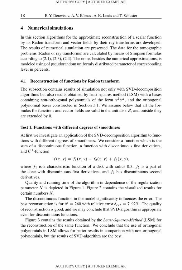
At first we investigate an application of the SVD-decomposition algorithm to func-tions with different degrees of smoothness. We consider a function which is thesum of a discontinuous function, a function with discontinuous first derivatives,and C 1-function

f .x; y/ D f1.x; y/C f2.x; y/C f3.x; y/;

where f1 is a characteristic function of a disk with radius 0:3, f2 is a part ofthe cone with discontinuous first derivatives, and f3 has discontinuous secondderivatives.

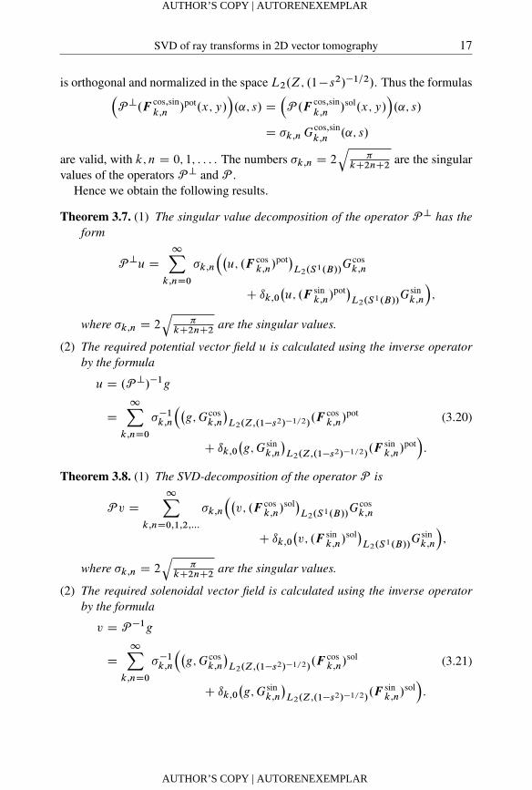
Quality and running time of the algorithm in dependence of the regularizationparameter N is depicted in Figure 1. Figure 2 contains the visualized results forcertain numbers N .

The discontinuous function in the model significantly influences the error. Thebest reconstruction is for N D 260 with relative error ırel D 7; 92%. The qualityof reconstruction is good, and we may conclude that SVD-algorithm is appropriateeven for discontinuous functions.

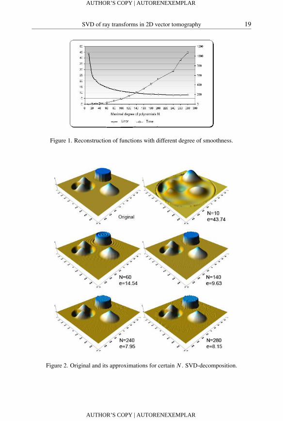
Figure 3 contains the results obtained by the Least-Squares-Method (LSM) forthe reconstruction of the same function. We conclude that the use of orthogonalpolynomials in LSM allows for better results in comparison with non-orthogonalpolynomials, but the results of SVD-algorithm are the best.




Figure 1. Reconstruction of functions with different degree of smoothness.

Figure 2. Original and its approximations for certain N . SVD-decomposition.




Figure 3. Reconstruction of the function by LSM-algorithm.

4.2 Reconstruction of vector fields

The behavior of the SVD-algorithm applied to vector fields reconstruction is sim-ilar to the reconstruction of a scalar function so we restrict ourselves to only onenumerical test which is devoted to the influence of the noise level to the quality ofreconstruction. The conclusions from analyzing the results are valid not only forvector fields reconstruction but for reconstruction of the functions, too.

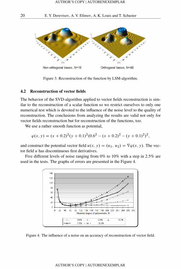
We use a rather smooth function as potential,

'.x; y/ D .x C 0:2/2.y C 0:1/2.0:62 � .x C 0:2/2 � .y C 0:1/2/2;

and construct the potential vector field u.x; y/ D .u1; u2/ D r'.x; y/. The vec-tor field u has discontinuous first derivatives.

Five different levels of noise ranging from 0% to 10% with a step in 2.5% areused in the tests. The graphs of errors are presented in the Figure 4.

Figure 4. The influence of a noise on an accuracy of reconstruction of vector field.




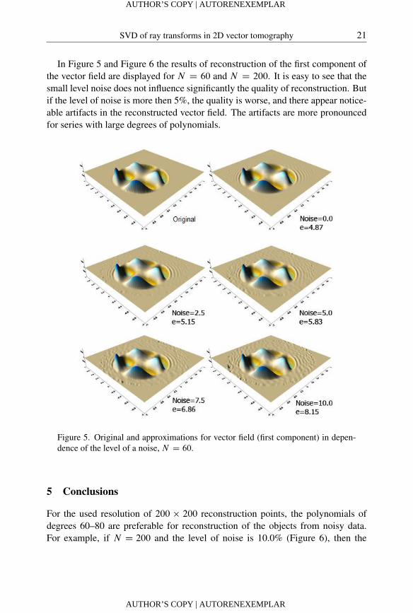
In Figure 5 and Figure 6 the results of reconstruction of the first component ofthe vector field are displayed for N D 60 and N D 200. It is easy to see that thesmall level noise does not influence significantly the quality of reconstruction. Butif the level of noise is more then 5%, the quality is worse, and there appear notice-able artifacts in the reconstructed vector field. The artifacts are more pronouncedfor series with large degrees of polynomials.

Figure 5. Original and approximations for vector field (first component) in depen-dence of the level of a noise, N D 60.

5 Conclusions

For the used resolution of 200 � 200 reconstruction points, the polynomials ofdegrees 60–80 are preferable for reconstruction of the objects from noisy data.For example, if N D 200 and the level of noise is 10.0% (Figure 6), then the




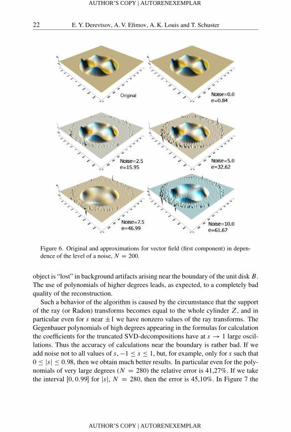
Figure 6. Original and approximations for vector field (first component) in depen-dence of the level of a noise, N D 200.

object is “lost” in background artifacts arising near the boundary of the unit diskB .The use of polynomials of higher degrees leads, as expected, to a completely badquality of the reconstruction.

Such a behavior of the algorithm is caused by the circumstance that the supportof the ray (or Radon) transforms becomes equal to the whole cylinder Z, and inparticular even for s near ˙1 we have nonzero values of the ray transforms. TheGegenbauer polynomials of high degrees appearing in the formulas for calculationthe coefficients for the truncated SVD-decompositions have at s ! 1 large oscil-lations. Thus the accuracy of calculations near the boundary is rather bad. If weadd noise not to all values of s, �1 � s � 1, but, for example, only for s such that0 � jsj � 0:98, then we obtain much better results. In particular even for the poly-nomials of very large degrees (N D 280) the relative error is 41,27%. If we takethe interval Œ0; 0:99� for jsj, N D 280, then the error is 45,10%. In Figure 7 the




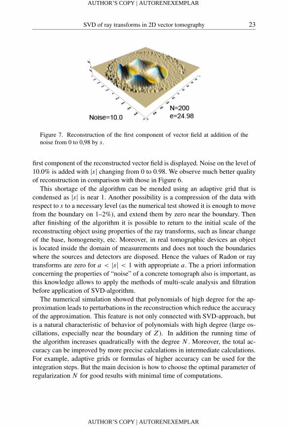
Figure 7. Reconstruction of the first component of vector field at addition of thenoise from 0 to 0,98 by s.

first component of the reconstructed vector field is displayed. Noise on the level of10.0% is added with jsj changing from 0 to 0.98. We observe much better qualityof reconstruction in comparison with those in Figure 6.

This shortage of the algorithm can be mended using an adaptive grid that iscondensed as jsj is near 1. Another possibility is a compression of the data withrespect to s to a necessary level (as the numerical test showed it is enough to movefrom the boundary on 1–2%), and extend them by zero near the boundary. Thenafter finishing of the algorithm it is possible to return to the initial scale of thereconstructing object using properties of the ray transforms, such as linear changeof the base, homogeneity, etc. Moreover, in real tomographic devices an objectis located inside the domain of measurements and does not touch the boundarieswhere the sources and detectors are disposed. Hence the values of Radon or raytransforms are zero for a < jsj < 1 with appropriate a. The a priori informationconcerning the properties of “noise” of a concrete tomograph also is important, asthis knowledge allows to apply the methods of multi-scale analysis and filtrationbefore application of SVD-algorithm.

The numerical simulation showed that polynomials of high degree for the ap-proximation leads to perturbations in the reconstruction which reduce the accuracyof the approximation. This feature is not only connected with SVD-approach, butis a natural characteristic of behavior of polynomials with high degree (large os-cillations, especially near the boundary of Z). In addition the running time ofthe algorithm increases quadratically with the degree N . Moreover, the total ac-curacy can be improved by more precise calculations in intermediate calculations.For example, adaptive grids or formulas of higher accuracy can be used for theintegration steps. But the main decision is how to choose the optimal parameter ofregularization N for good results with minimal time of computations.




A Appendix: Classical orthogonal polynomials

For the construction of the bases as well as in original spaces as in the spaces ofimages of the operators of Radon and ray transform, we need special polynomialsdepending on one or two variables. They are harmonic polynomials, Jacobi andGegenbauer polynomials. We list their main properties used in the paper.

A.1 Harmonic polynomials

Let us consider harmonic polynomials of two variables given in a unit disk B . Bydefinition they are solutions of the Laplace equation

4H.x; y/ D 0:

In polar coordinate system .r; '/ they may be written in the form

H cosk .r; '/ D rk cos k';

H sink .r; '/ D rk sin k';

(A.1)

where k is a degree of the polynomial. For harmonics of degree zero (k D 0) wedefine

H cos0 .r; '/ D H sin

0 .r; '/def�

1p2: (A.2)

The bases for vector fields are constructed by differentiation of potentials, con-taining harmonic polynomials therefor there are useful relations allowing to cal-culate their derivatives

@

@xH cosk D kH

cosk�1;

@

@xH sink D kH

sink�1;

@

@yH cosk D �kH

sink�1;

@

@yH sink D kH

cosk�1:

(A.3)

A.2 Jacobi polynomials for the interval .0; 1/

The Jacobi polynomials given on the interval .0; 1/ are calculated according to theformula

P .p;q/n .t/ D 1C

nXkD1

.�1/kC kn.p C n/.p C nC 1/ : : : .p C nC k � 1/

q.q C 1/ : : : .q C k � 1/tk :




On the interval .0; 1/ the polynomials are orthogonal with a weight tq�1.1�t /p�q ,Z 1

0

tq�1.1 � t /p�qP .p;q/n .t/P .p;q/m .t/dt

DnŠ�.q/�.p � q C nC 1/

q.q C 1/ : : : .q C n � 1/.p C 2n/�.p C n/ınm;

(A.4)

where ınm is the Kronecker symbol.The bases for vector fields are constructed by differentiation of potentials, con-

taining not only harmonic polynomials, but Jacobi polynomials too. There are use-ful relations allowing to calculate their derivatives

d

dt

�P .p;q/n .t/

�D �

n.nC p/

qP.pC2;qC1/n�1 .t/: (A.5)

A.3 Gegenbauer polynomials for the interval .�1; 1/

The Gegenbauer polynomials C .�/n .t/ are the main tool for constructing bases inspaces of images of Radon and ray transforms. They are determined by the formula

C .�/n .t/ D1

�.�/

Œn2�X

kD0

.�1/k�.�C n � k/

kŠ.n � 2k/Š.2t/n�2k :

The polynomials are orthogonal with a weight .1�t2/��1=2 on the interval .�1;1/,Z 1

�1

C .�/n .t/C .�/m .t/.1 � t2/��1=2dt D�21�2��.nC 2�/

nŠ.nC �/�2.�/ınm: (A.6)

Recurrence formulas are

.nC 1/C.�/nC1.t/ � 2�

�tC .�C1/n .t/ � C

.�C1/n�1 .t/

�D 0; (A.7)

.nC 2�/C .�/n .t/ � 2��C .�C1/n .t/ � tC

.�C1/n�1 .t/

�D 0; (A.8)

and the derivatives fulfill

.1 � t2/dC

.�/n .t/

dtD .nC 2� � 1/C

.�/n�1.t/ � ntC

.�/n .t/

D .nC 2�/tC .�/n .t/ � .nC 1/C.�/nC1.t/:

(A.9)




Bibliography

[1] M. Abramowitz and I. A. Stegun, Handbook of Mathematical Functions, NationalBureau of Standards Applied Mathematics Series, John Wiley & Sons, New York,1972.

[2] A. M. Cormack, Representations of a function by its line integrals with some radio-logical applications II, J. Appl. Physics 35 (1964), 2908–2913.

[3] M. E. Davison, A singular value decomposition for the Radon transform in n-dimen-sional Euclidean space, Numer. Funct. Anal. Optim. 3 (1981), 321–340.

[4] E. Y. Derevtsov, Certain problems of non-scalar tomography, Sib. Èlektron. Mat. Izv.7 (2010), C.81–C.111 (in Russian).

[5] E. Y. Derevtsov, S. G. Kazantsev and T. Schuster, Polynomial bases for subspaces ofvector fields in the unit ball. Method of ridge functions, J. Inverse Ill-Posed Probl. 5(2007), no. 1, 1–38.

[6] E. Y. Derevtsov, V. V. Pickalov and T. Schuster, Application of local operators fornumerical reconstruction of a singular support of a vector field by its known raytransforms, J. Phys. Conf. Ser. 135 (2008), Article ID 012035.

[7] I. C. Gohberg and M. G. Krein, Introduction to the Theory of Linear NonselfadjointOperators, American Mathematical Society, Providence, RI, 1969.

[8] S. G. Kazantsev and A. A. Bukhgeim, Singular value decomposition for the 2D fan-beam Radon transform of tensor fields, J. Inverse Ill-Posed Probl. 12 (2004), no. 4,1–35.

[9] N. E. Kochin Vector Calculus and Fundamentals of Tensor Calculus, ONTI, Gos.tekhniko-teoreticheskoe izd., Leningrad, Moscow, 1934 (in Russian).

[10] A. K. Louis, Orthogonal function series expansions and the null space of the Radontransform, SIAM J. Math. Anal. 15 (1984), 621–633.

[11] A. K. Louis, Tikhonov–Phillips regularization of the Radon transform, in: Construc-tive Methods for the Practical Treatment of Integral Equations, pp. 211–223, editedby G. Hämmerlin and K.-H. Hoffman, Birkhäuser-Verlag, Basel, 1985.

[12] A. K. Louis, Incomplete data problems in X-ray computerized tomography I: Sin-gular value decomposition of the limited angle transform, Numer. Math. 48 (1986),251–262.

[13] A. K. Louis, Inverse und schlecht gestellte Probleme, B. G. Teubner, Stuttgart, 1989.

[14] A. K. Louis, Feature reconstruction in inverse problems, Inverse Problems 27 (2011),065010, DOI:10.1088/0266-5611/27/6/065010.

[15] A. K. Louis and T. Schuster, A novel filter design technique in 2D X-ray CT, InverseProblems 12 (1996), 685–696.

[16] P. Maass, The X-ray transform: Singular value decomposition and resolution, InverseProblems 3 (1987), 727–741.




[17] R. B. Marr, On the reconstruction of a function on a circular domain from a samplingof its line integrals, J. Math. Anal. Appl. 19 (1974), 357–374.

[18] F. Natterer, The Mathematics of Computerized Tomography, B. G. Teubner, Stuttgart,John Wiley & Sons, Chichester, 1986.

[19] E. T. Quinto, Singular value decomposition and inversion methods for the exteriorRadon transform and a spherical transform, J. Math. Anal. Appl. 95 (1985), 437–448.

[20] T. Schuster, The 3D Doppler transform: Elementary properties and computation ofreconstruction kernels, Inverse Problems 16 (2000), no. 3, 701–723.

[21] T. Schuster, An efficient mollifier method for three-dimensional vector tomography:Convergence analysis and implementation, Inverse Problems 17 (2001), 739–766.

[22] T. Schuster, The Method of Approximate Inverse: Theory and Applications, LectureNotes in Mathematics 1906, Springer-Verlag, Heidelberg, 2007.

[23] V. A. Sharafutdinov, Integral Geometry of Tensor Fields, VSP, Utrecht, 1994.

[24] G. Szego, Orthogonal Polynomials, American Mathematical Society, Providence,RI, 1939.

[25] H. Weyl, The method of orthogonal projection in potential theory, Duke Math. J. 7(1940), 411–444.

Received August 5, 2011.

Author information

Evgeny Y. Derevtsov, Sobolev Institute of Mathematics,Acad. Koptyug prosp., 4, 630090 Novosibirsk, Russia.E-mail: [email protected]

Anton V. Efimov, Novosibirsk State University,Pirogova St., 2, 630090 Novosibirsk, Russia.E-mail: [email protected]

Alfred K. Louis, Institute of Applied Mathematics, Saarland University,66041 Saarbrücken, Germany.E-mail: [email protected]

Thomas Schuster, Department for Mathematics,Carl von Ossietzky University Oldenburg, 26129 Oldenburg, Germany.E-mail: [email protected]



mailto:[email protected]




singular value decomposition and its application to

Documents