Lecture 11

Vector Spacesand

Singular Value Decomposition

SyllabusLecture 01 Describing Inverse ProblemsLecture 02 Probability and Measurement Error, Part 1Lecture 03 Probability and Measurement Error, Part 2 Lecture 04 The L2 Norm and Simple Least SquaresLecture 05 A Priori Information and Weighted Least SquaredLecture 06 Resolution and Generalized InversesLecture 07 Backus-Gilbert Inverse and the Trade Off of Resolution and VarianceLecture 08 The Principle of Maximum LikelihoodLecture 09 Inexact TheoriesLecture 10 Nonuniqueness and Localized AveragesLecture 11 Vector Spaces and Singular Value DecompositionLecture 12 Equality and Inequality ConstraintsLecture 13 L1 , L∞ Norm Problems and Linear ProgrammingLecture 14 Nonlinear Problems: Grid and Monte Carlo Searches Lecture 15 Nonlinear Problems: Newton’s Method Lecture 16 Nonlinear Problems: Simulated Annealing and Bootstrap Confidence Intervals Lecture 17 Factor AnalysisLecture 18 Varimax Factors, Empirical Orthogonal FunctionsLecture 19 Backus-Gilbert Theory for Continuous Problems; Radon’s ProblemLecture 20 Linear Operators and Their AdjointsLecture 21 Fréchet DerivativesLecture 22 Exemplary Inverse Problems, incl. Filter DesignLecture 23 Exemplary Inverse Problems, incl. Earthquake LocationLecture 24 Exemplary Inverse Problems, incl. Vibrational Problems

Purpose of the Lecture

View m and d as points in thespace of model parameters and data

Develop the idea of transformations of coordinate axes

Show how transformations can be used to convert a weighted problem into an unweighted one

Introduce the Natural Solution and the Singular Value Decomposition

Part 1

the spaces ofmodel parameters

anddata

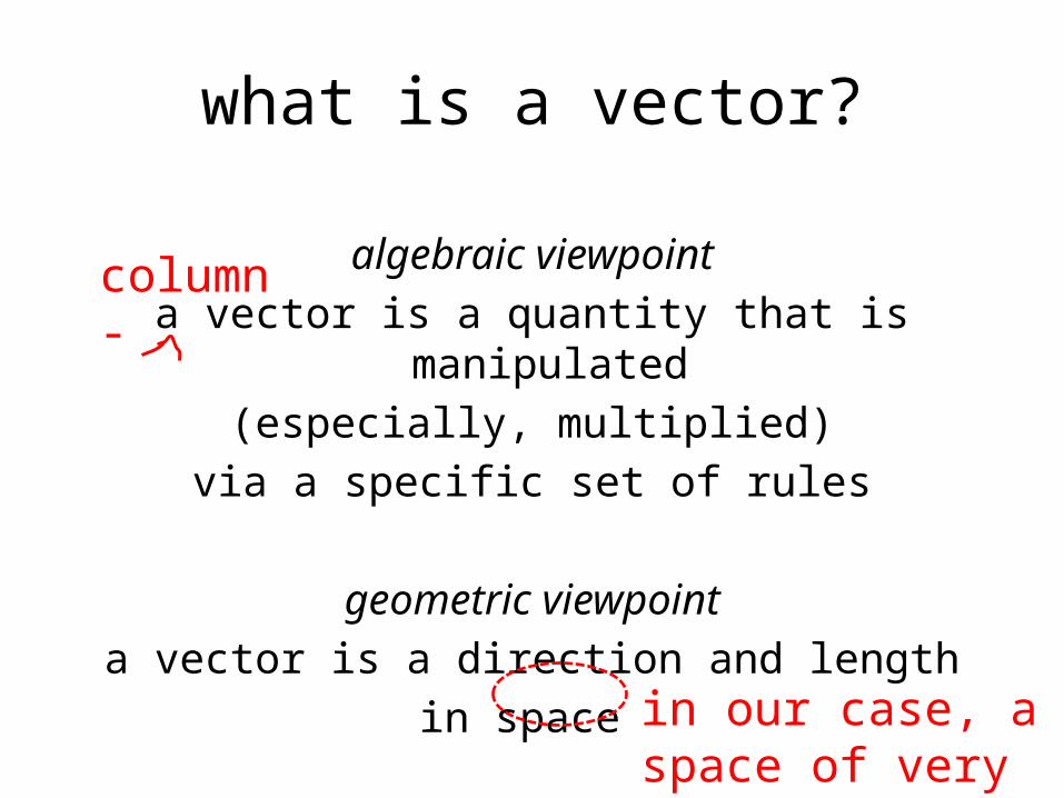
what is a vector?

algebraic viewpoint

a vector is a quantity that is manipulated

(especially, multiplied)

via a specific set of rules

geometric viewpoint

a vector is a direction and length

in space

what is a vector?

algebraic viewpoint

a vector is a quantity that is manipulated

(especially, multiplied)

via a specific set of rules

geometric viewpoint

a vector is a direction and length

in space

column-

in our case, a space of very high dimension

S(m)m3

m2 m1 d1

d2d3

S(d)m d

forward problem

d = Gmmaps an m onto a d

maps a point in S(m) to a point in S(d)

m3

m2 m1 d1

d2d3m d

Forward Problem: Maps S(m) onto S(d)

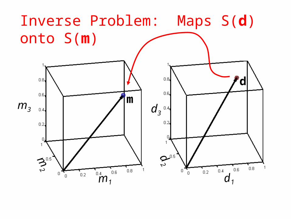
inverse problem

m = G-gdmaps a d onto an m

maps a point in S(m) to a point in S(d)

m3

m2 m1 d1

d2d3m d

Inverse Problem: Maps S(d) onto S(m)

Part 2

Transformations of coordinate axes

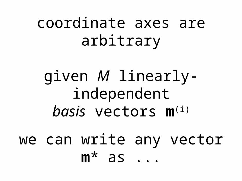
coordinate axes are arbitrary

given M linearly-independentbasis vectors m(i)

we can write any vector m* as ...

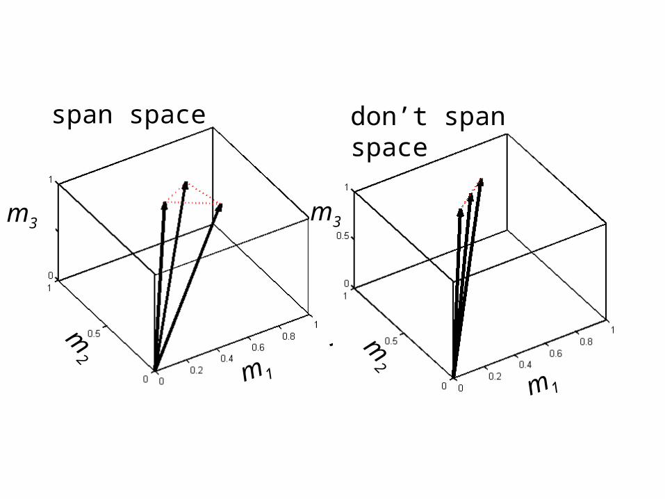
span space

m3

m2 m1m2

dm3

m1

m2

don’t span space

... as a linear combination of these basis vectors

... as a linear combination of these basis vectors

components of m* in new coordinate system

mi*’ = αi

might it be fair to saythat the components of a vector

are a column-vector?

matrix formed from basis vectorsMij = vj(i)

transformation matrix T

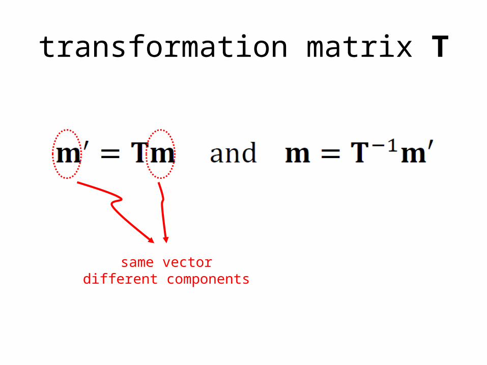
transformation matrix T

same vectordifferent components

Q: does T preserve “length” ?(in the sense that mTm = m’Tm’)

A: only when TT= T-1

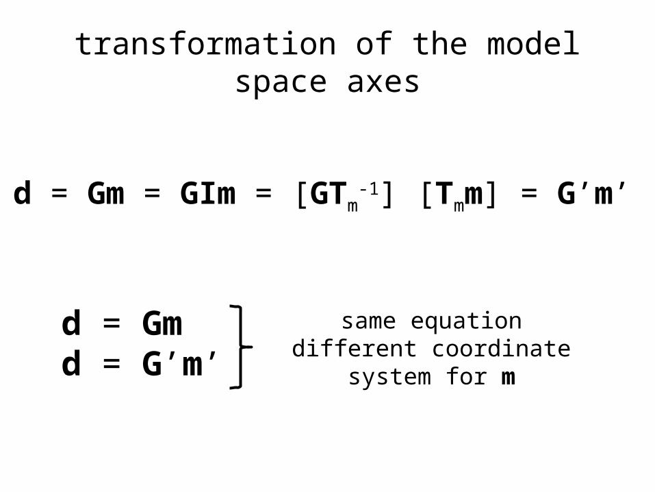
transformation of the model space axes

d = Gm = GIm = [GTm-1] [Tmm] = G’m’d = Gmd = G’m’ same equation

different coordinate system for m

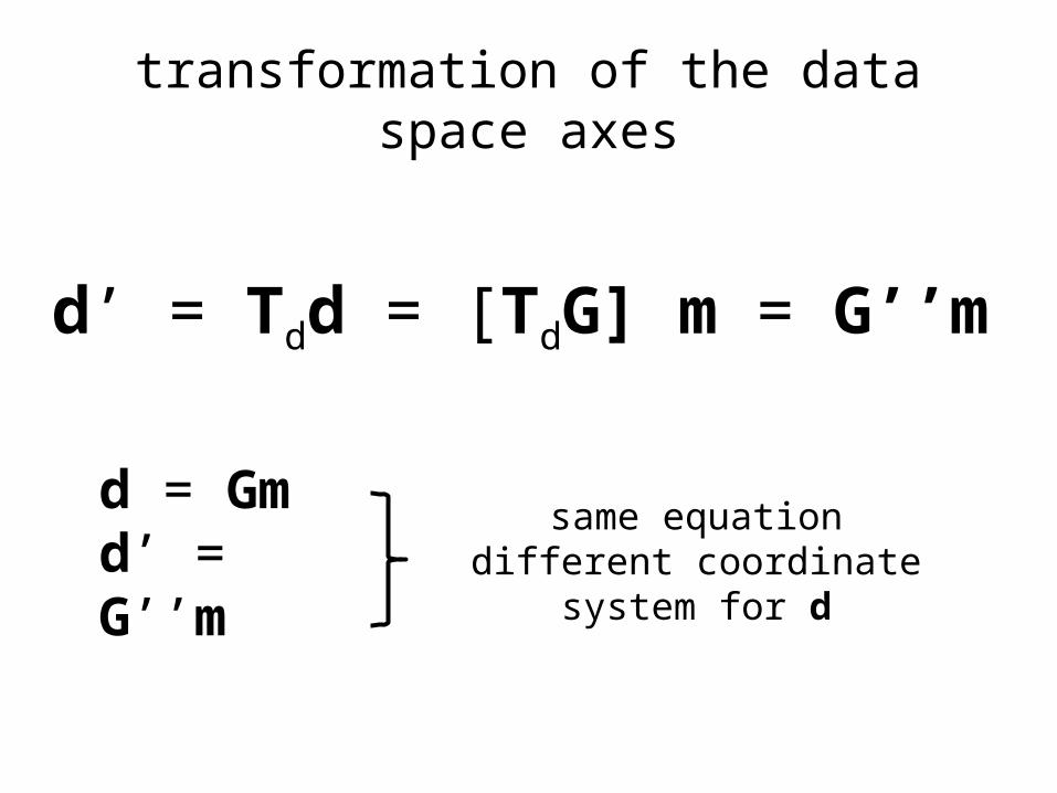
transformation of the data space axes

d’ = Tdd = [TdG] m = G’’md = Gmd’ = G’’m same equation

different coordinate system for d

transformation of both data space and model space axes

d’ = Tdd = [TdGTm-1] [Tmm] = G’’’m’d = Gmd’ = G’’’m’ same equation

different coordinate systems for d and m

Part 3

how transformations can be used to convert a weighted problem into

an unweighted one

when are transformations useful ?

remember this?

when are transformations useful ?

remember this?

massage this into a pair of transformations

mTWmmWm=DTD or Wm=Wm½Wm½=Wm T½ Wm½

OK since Wm symmetric

mTWmm = mTDTDm = [Dm] T[Dm] Tm

when are transformations useful ?

remember this?

massage this into a pair of transformations

eTWeeWe=We½We½=We T½ We½

OK since We symmetric

eTWee = eTWe T½ We½e = [We½m] T[We½m] Td

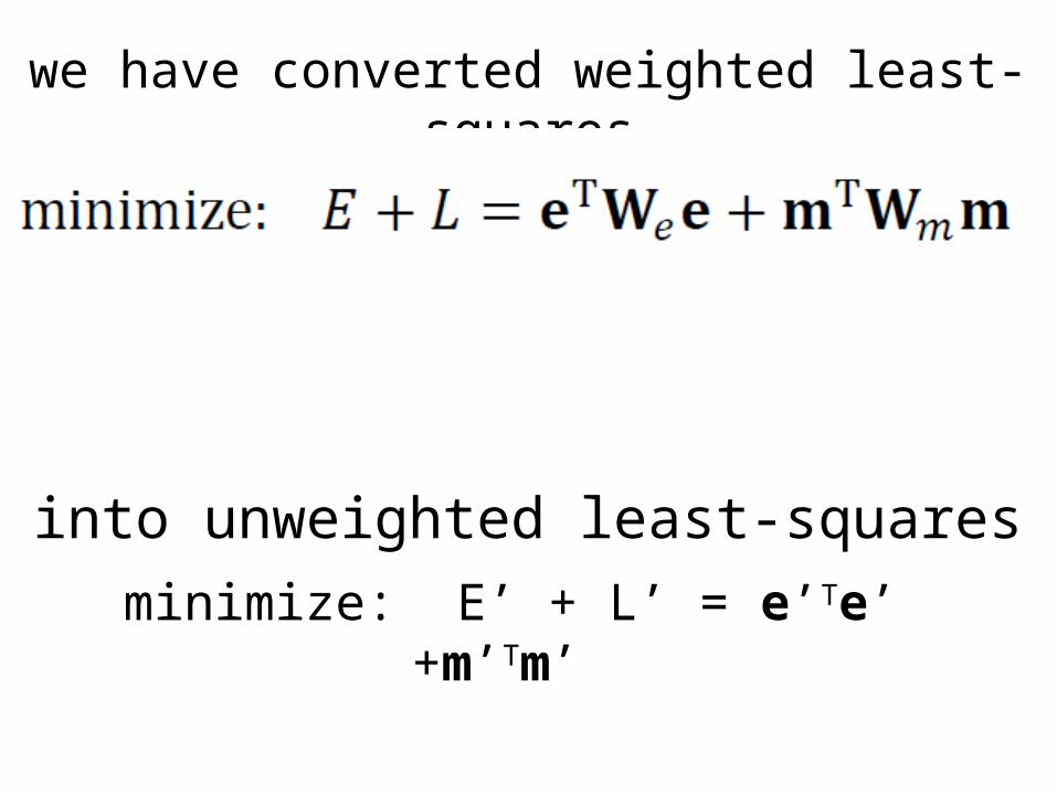
we have converted weighted least-squares

minimize: E’ + L’ = e’Te’ +m’Tm’ into unweighted least-squares

steps

1: Compute Transformations

Tm=D=Wm½ and Te=We½2: Transform data kernel and data to new coordinate system

G’’’=[TeGTm-1] and d’=Ted3: solve G’’’ m’ = d’ for m’ using unweighted method

4: Transform m’ back to original coordinate system

m=Tm-1m’

steps

1: Compute Transformations

Tm=D=Wm½ and Te=We½2: Transform data kernel and data to new coordinate system

G’’’=[TeGTm-1] and d’=Ted3: solve G’’’ m’ = d’ for m’ using unweighted method

4: Transform m’ back to original coordinate system

m=Tm-1m’

extra work

steps

1: Compute Transformations

Tm=D=Wm½ and Te=We½2: Transform data kernel and data to new coordinate system

G’’’=[TeGTm-1] and d’=Ted3: solve G’’’ m’ = d’ for m’ using unweighted method

4: Transform m’ back to original coordinate system

m=Tm-1m’

to allow simpler solution method

Part 4

The Natural Solution and the Singular Value Decomposition

(SVD)

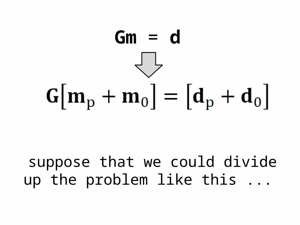
Gm = d

suppose that we could divide up the problem like this ...

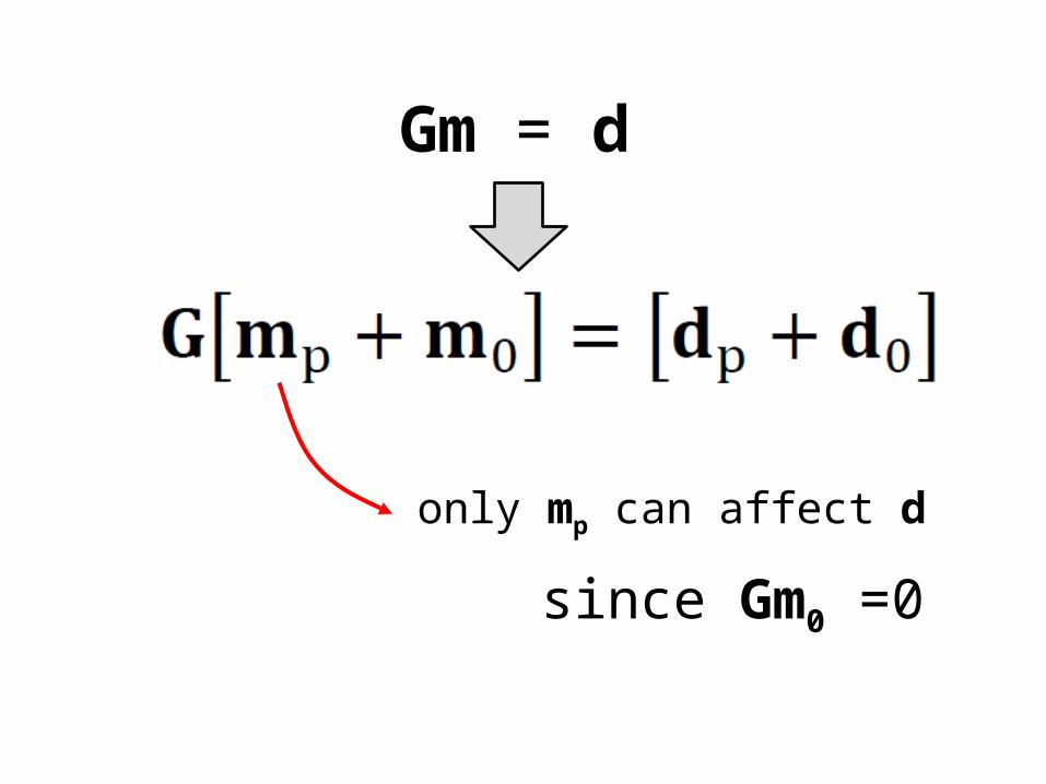
Gm = d

only mp can affect dsince Gm0 =0

Gm = d

Gmp can only affect dpsince no m can lead

to a d0

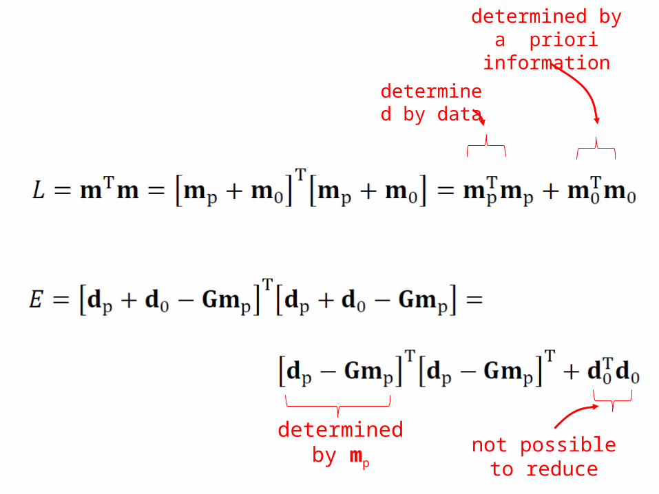
determined by data

determined by a priori information

determined by mp not possible to reduce

natural solution

determine mp by solving dp-Gmp=0set m0=0

what we need is a way to do

Gm = d

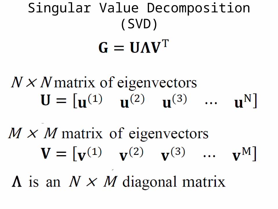
Singular Value Decomposition (SVD)

singular value decomposition

UTU=I and VTV=I

suppose only p λ’s are non-zero

suppose only p λ’s are non-zero

only first p columns of U

only first p columns of V

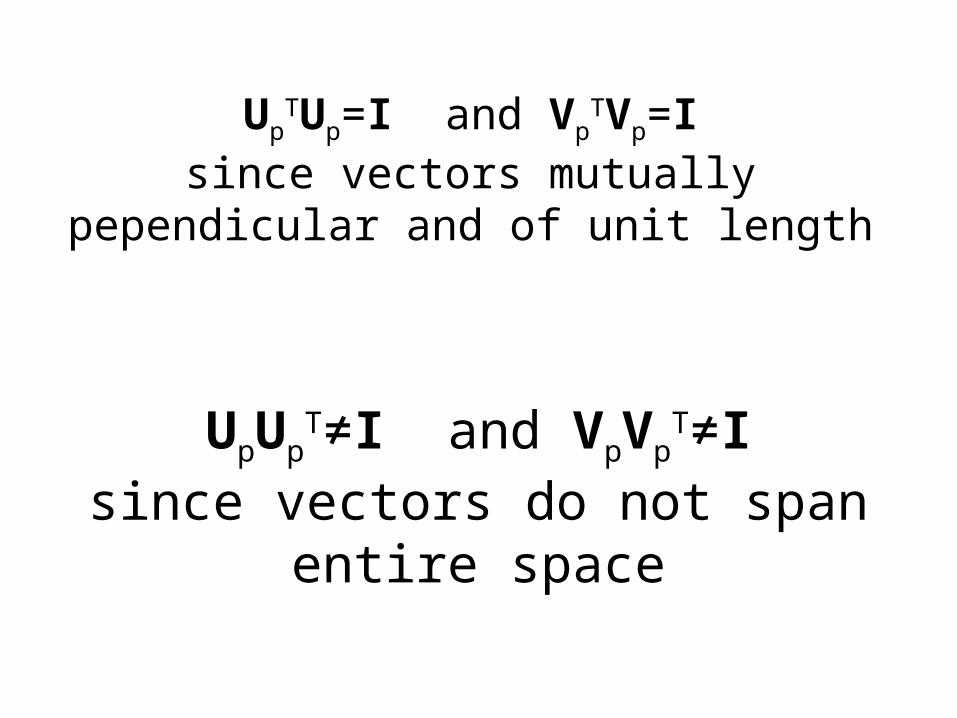
UpTUp=I and Vp

TVp=Isince vectors mutually pependicular

and of unit length

UpUpT≠I and VpVp

T≠Isince vectors do not span entire space

The part of m that lies in V0 cannot effect d

since VpTV0=0so V0 is the model null space

The part of d that lies in U0 cannot be affected by m

since ΛpVpTm is multiplied by Upand U0 UpT =0

so U0 is the data null space

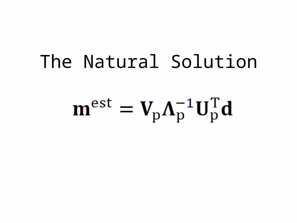
The Natural Solution

The part of mest in V0 has zero length

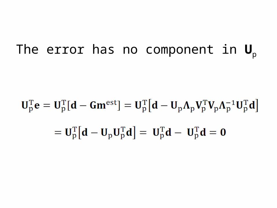
The error has no component in Up

computing the SVD

determining puse plot of λi vs. i

however

case of a clear division betweenλi>0 and λi=0 rare

2 4 6 8 10 12 14 16 18 200

1

2

3

4

iS

i

2 4 6 8 10 12 14 16 18 200

0.5

1

1.5

2

2.5

i

Si

(A) (B)

(C) (D)

ji

ji

index number, iλi

λi

index number, iλi

p

p?

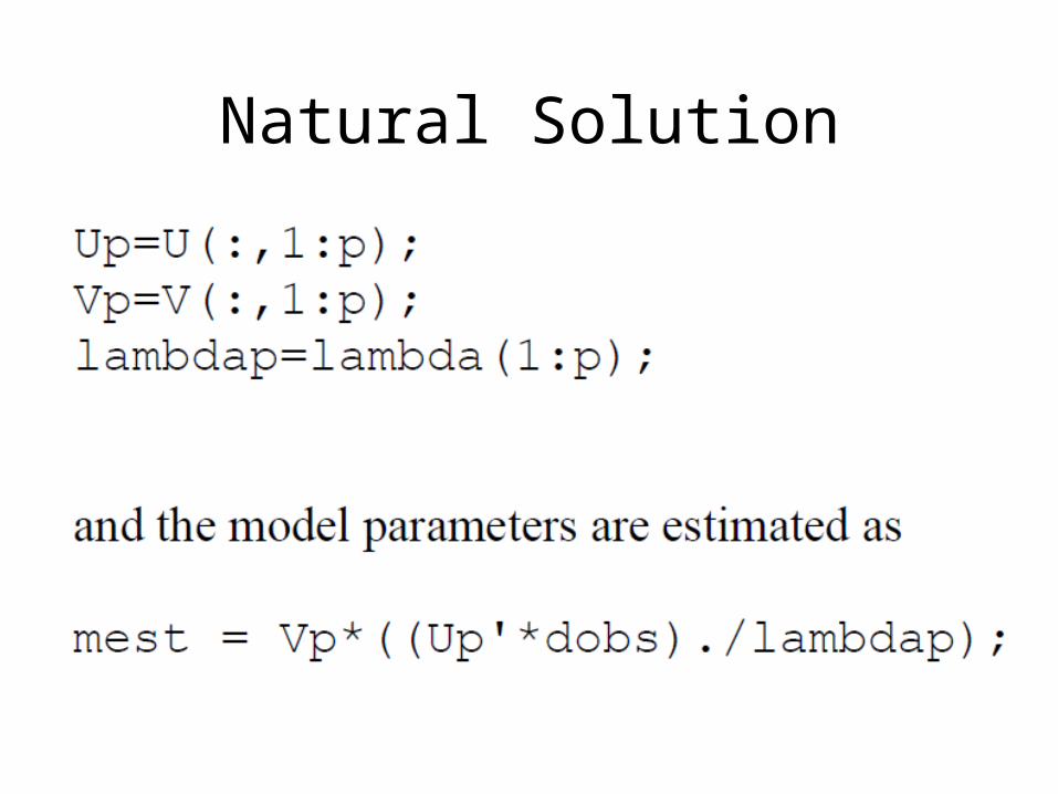
Natural Solution

=

(A) (B)

G m dobs mtrue (mest)N(mest)DML

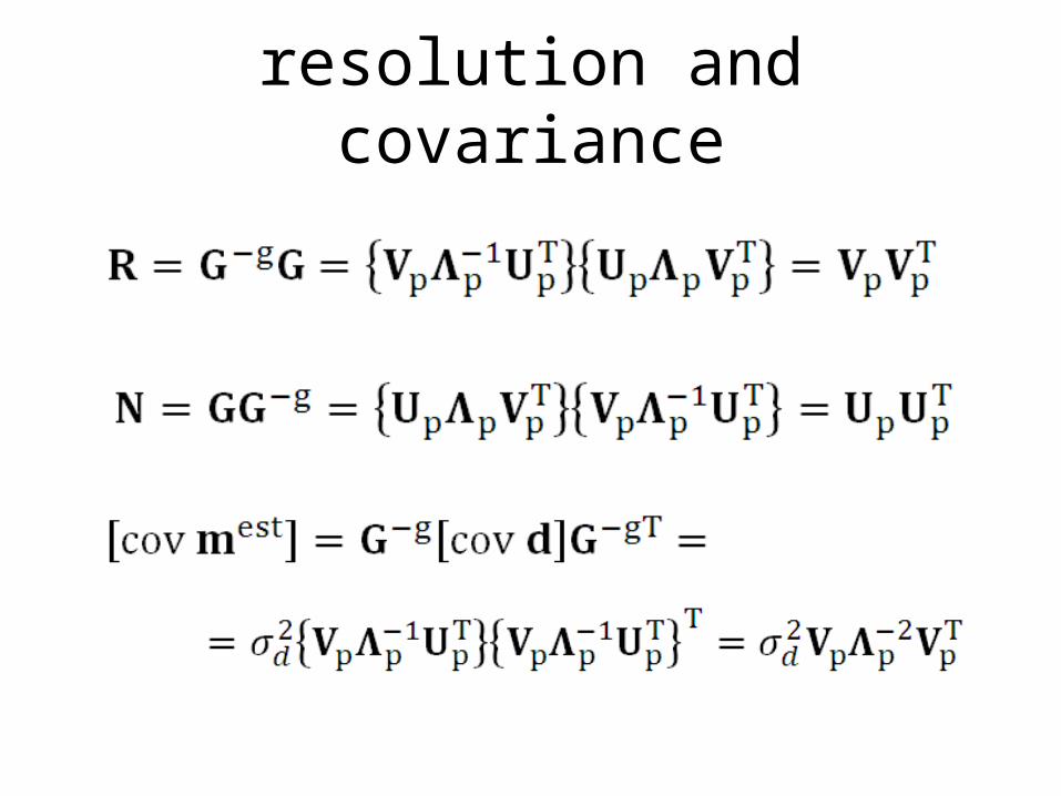
resolution and covariance

resolution and covariance

large covariance if any λp are small

Is the Natural Solution the best solution?

Why restrict a priori information to the null space

when the data are known to be in error?

A solution that has slightly worse error but fits the a priori information better might be preferred ...