how big are the environmental benefits of high-speed rail

How Big Are the Environmental Benefits of High-Speed Rail? A Cost-Benefit Analysis of High-Speed Rail replacing automobile travel in the Georgetown-San Antonio corridor.

By

Kevin Scott

An Applied Research Project (Political Science 5397)

Submitted to the Department of Political Science Texas State University

In Partial Fulfillment for the Requirements for the Degree of Masters of Public Administration

Fall 2011

Faculty Approval:

Dr. Hassan Tajalli

Dr. Willard Fields

Jared Gallini MPA

Abstract

Purpose. The purpose of this study is to determine the environmental impact of a high-speed rail

network operating in the Georgetown-San Antonio corridor Methods. This research uses a cost-

benefit analysis methodology in order to determine whether high-speed rail will reduce the

annual carbon dioxide levels produced by automobiles in the Georgetown-San Antonio corridor.

The data used for this study derive from existing published studies. The study then compares five

types of high-speed rail technologies that are planned for use in the United States to determine

which option has the lowest annual output of CO2 during operation. Results. The results show

that high-speed rail significantly reduces annual carbon dioxide levels within the corridor due to

the cancelling out of annual automobile trips in the Georgetown-San Antonio corridor. The

German Intercity Express (ICE) is found to be the appropriate high-speed rail technology to have

operating in the corridor, in producing the lowest annual emission cost of carbon dioxide of the

five high-speed rail technologies. Conclusion. Operation of a German Intercity Express (ICE)

high-speed rail network would benefit communities in the Georgetown-San Antonio corridor by

reducing the annual amount of automobile carbon dioxide emissions.

TABLE OF CONTENTS

CHAPTER ONE: INTRODUCTION…………………………………………………………..1

RESEARCH PURPOSE…………………………………………………………………………3 CHAPTERS SUMMARIES……………………………………………………………………3 CHAPTER TWO: LITERATURE REVIEW………………………………………………...5 HIGH SPEED RAIL TRANSFORMING THE UNITED STATES’ TRANSPORTATION SYSTEM…………………………………………………………………………………………..5

Recovery and Reinvestment Act…………………………………………………………6 Benefits available to United States Cities………………………………………………7

HIGH SPEED RAIL- TRAFFIC CONGESTION AND ITS COSTS…………………………8 Wasted travel hours and Fuel……………………………………………………………8 Roadways and Airport Congestion……………………………………………………...9 Japanese high-speed rail train Kyushu Shinkansen……………………………………..9 Congestion in Texas- Transportation Institute: 2009 urban mobility report……………11 Reduction in intercity trips & Short haul air travel……………………………………12

HIGH SPEED RAIL- INFLUENCE ON CLIMATE CHANGE AND OIL SCARCITY………13 Reduction of transportation emissions…………………………………………………..13 Reduce dependence on imported oil……………………………………………………..13

HIGH SPEED RAIL- environmentally friendly transit……………………………………14 Europe’s investments…………………………………………………………………….14 High speed rail versus Conventional rail energy consumption………………………15

HIGH-SPEED RAIL- SAFE, RELIABLE, AND ACCESSIBLE SOURCE OF TRANSPORTATION……………………………………………………………………………16

Proven safest mode of transportation……………………………………………………16 Accessible interconnected railway stations……………………………………………...18 Lone Star Rail……………………………………………………………………………19 Reduced travel times……………………………………………………………………20

HIGH SPEED RAIL- PROMOTES ECONOMIC DEVELOPMENT……………………….....20 Beneficial changes in local land use and national employment rates…………………20 Contributing to economic competitiveness, urban and rural growth……………………21 Tourism…………………………………………………………………………………..21 Annual increase in gross domestic product……………………………………………..22 DESIGNATED HIGH-SPEED RAIL TECHNOLOGIES…………………………….. 23 Shinkansen……………………………………………………………………….23 TGV………………………………………………………………………………….25 ICE……………………………………………………………………………………..25 IC-3……………………………………………………………………………………26 MagLev………………………………………………………………………… 27

CHAPTER SUMMARY……………………………………………………………………… 29 CONCEPTUAL FRAMEWORK……………………………………………………………….29

CHAPTER THREE: METHODOLOGY………………………………………………….....31

STATEMENT OF RESEARCH PURPOSE…………………………………………………….31 COSTS…………………………………………………………………………………………...32

Annual emission produced by high speed rail operation………………………………32 BENEFITS……………………………………………………………………………………….33

Reduction in annual carbon dioxide (CO2) level for corridor……………………………33 TIMEFRAME……………………………………………………………………………………33 OPERATIONALIZATION……………………………………………………………………...33 STRENGTHS AND WEAKNESSES OF A COST BENEFIT ANALYSIS………………36 DATA COLLECTION..................................................................................................................37 CALCULATING THE COST BENEFIT ANALYSIS………………………………………….38 BENEFITS……………………………………………………………………………………….38 Annual Weekday Vehicle Trip Cancellation…………………………………………….38 Annual commuter saves in automobile CO2……………………………………………41 Net annual automobile carbon dioxide emissions saved in the corridor………………..42 COSTS…………………………………………………………………………………………44

Individual commuter high-speed rail commuter costs in annual CO2 emission ...............44 Annual emission of CO2 for the five high-speed rail technologies………………….46

HUMAN SUBJECTS PROTECTION ………………………………………………………….49

CHAPTER FOUR: RESULTS……………………………………………………………...50

INTRODUCTION…………………………………………………………………………….…50 BENEFITS……………………………………………………………………………………….51

Direct Benefits…………………………………………………………………………...51 Vehicle Trip Cancellation………………………………………………………………..52 Average commuter saves annually of automobile carbon dioxide emission……..…55 Net Annual Automobile Emissions Saved……………………………………………57

COSTS…………………………………………………………………………………………...62 Individual commuter costs in annual CO2 emission by using high-speed rail…………...62

Annual emission of CO2 for each of the five high-speed rail technologies…………65 MODEL RESULTS……………………………………………………………………………69 CONCLUSION……………………………………………………………………………….72

CHAPTER FIVE: CONCLUSION………………………………………………………....73

INTRODUCTION……………………………………………………………………………….73 SUMMARY……………………………………………………………………………………...73 RECOMMENDATIONS………………………………………………………………………...75

BIBLIOGRAPHY………………………………………………………………………77 APPENDICIES APPENDIX-A: Map of proposed lone star commuter rail…………………………..……...…...82 APPENDIX-B: Map of United States’ petroleum imports …………………...…………………83 APPENDIX-C: U.S. Traffic and fatality rates-1990-2009 per 100 million miles traveled……84

APPENDIX-D: Average distance traveled between destinations, Number of daily riders, Average daily miles driven by riders from each station, Daily number of car trip cancelled, Average auto occupancy……………………………………..………………….85 List of Images, Tables

CHAPTER 2

Image 2.1: High-Speed Intercity Passenger Rail Program................................................6 Table 2.1: Shinkansen CO2 emission data……………………………………………24 Table 2.2: TGV CO2 emission data…………………………………………………….25 Table 2.3: ICE CO2 emission data……………………………………………………26 Table 2.4: IC-3 CO2 emission data……………………………………………………27 Table 2.5: MagLev CO2 emission data…………………………………………………28 Table 2.6: Conceptual framework of scholarly research……………..……………….30

CHAPTER 3

Table 3.1: Operationalization of the Conceptual Framework Table..................................35 Table 3.2: Weekday ridership estimate for the corridor………………………………....39 Table 3.3: Average automobile occupancy………………………………………………40 Table 3.4: Annual weekday vehicle trip cancellation for the corridor…………………..40

Table 3.5: Average automobile’s emission of CO2 per passenger mile………………...41 Table 3.6: Annual commuter savings in automobile carbon dioxide………….. 42 Table 3.7: Net Annual Automobile Carbon Dioxide Emissions Saved in the Corridor...44 Table 3.8: CO2 emission rate per passenger mile based on five high-speed rail options..45 Table 3.9: Individual commuter costs in annual high-speed rail CO2……………….46 Table 3.10: CO2 rate per passenger mile on five high-speed rail options……………47 Table 3.11: Average daily miles by riders in the Georgetown-San Antonio corridor…..47 Table 3.12: High-speed rail annual emissions on high-speed technology selected……48

CHAPTER 4 Table 4.1: Average weekday commuter trips diverted in favor of rail ……………….52 Table 4.2: Average automobile occupancy by daily trip purpose……………………..53

Table 4.3: Annual weekday vehicle trip cancellation for the corridor……………….54 Table 4.4: Summary CO2 Emissions Factors by Mode………………………………..55

Table 4.5: Average daily miles by riders in the Georgetown-San Antonio corridor…..56 Table 4.6: Formula to calculate the annual commuter’s savings of automobile CO2………57 Table 4.7: Average daily miles by riders in the Georgetown-San Antonio corridor…….58 Table 4.8: Average automobile occupancy……………………………………………58 Table 4.9: Summary CO2 Emissions Factors by Mode………………………………59 Table 4.10: Annual savings of automobile CO2 emissions in corridor…………………..60 Table 4.11: Annual automobile emissions saved by station and corridor……………….61 Table 4.12: CO2 emission rate per passenger mile based on five high-speed rail option..62

Table 4.13: average distance between Georgetown-San Antonio corridor rail stations…63 Table 4.14: Commuter’s annual emission footprint by high-speed rail technology…….64 Table 4.15: Annual emission using each of the five high-speed technologies…………..64 Table 4.16: Five high-speed rail technologies’ CO2 lbs per passenger mile…………….66 Table 4.17: Average daily miles by riders in the Georgetown-San Antonio corridor.......66 Table 4.18: Formula determining high-speed annual emissions footprint……………67 Table 4.19: Five high-speed rail technologies’ annual emissions……………………68 Table 4.20: Net annual emissions savings for Georgetown-San Antonio corridor……69 Table 4.21: Annual automobile emissions saved by station and corridor……………….70 Table 4.22: Five high-speed rail technologies’ annual emission ………………………71 Table 4.23: Total annual net emissions savings by high-speed rail technology……….71

About the Author

Kevin Scott earned his Masters of Public Administration candidate from Texas State

University in San Marcos. He completed his undergraduate studies at Texas State University in

San Marcos, earning a Bachelor of Applied Arts in Public Administration in 2009. His interest in

high-speed rail came from his major focus in Urban and Environmental Planning during graduate

and undergraduate studies, along with his time as an intern at the Texas Commission on

Environmental Quality. He has lived and worked in the I.H. 35 corridor and during this time

observed the population / urban growth and related Environmental, Transportation and Economic

impacts. These impacts have influenced his interest in Environmental and Transportation related

issues. Mr. Scott Lives in New Braunfels, Texas and can be reached by email at

[email protected]

mailto:[email protected]

1

Chapter 1: INTRODUCTION

Introduction

The United States Government spends billions of dollars annually on highways and

public transit systems, but traffic congestion remains. Rush hour in many cities now lasts all

morning and afternoon, reaching far into surrounding suburbs. Traffic tie-ups cost motorists at

least $74 billion every year in wasted time and fuel (Hosansky 1999, 729).

Of the 1,700 mile length of Interstate 35 from Mexico to Canada, the section with the

highest levels of fatalities, the worst congestion, the slowest average speed per mile, and the

highest levels of air pollution is the Georgetown-San Antonio corridor (Austin-San Antonio

Commuter Rail District 2003, 1). These problems occur in part due to the population boom along

the Georgetown-San Antonio corridor. Experts expect the corridor’s population to double almost

five million people - the size of the Dallas-Ft. Worth metroplex by the year 2023 (Austin-San

Antonio Commuter Rail District 2003, 1). The construction, maintenance and improvement of I-

35 required to accommodate current and future traffic will take decades to complete causing

further traffic delays. The Texas Department of Transportation’s attempt to help divert the

amount of traffic on I-35 has been to add toll roads along the Georgetown-San Antonio corridor.

The effect has been positive, with freight vehicle traffic now using the State highway 130 toll

way; but, the toll ways have had a limited impact on the daily commuter traffic and congestion

continues to be a daily problem. Texas Legislature and relevant State and Federal Agencies

should review alternative modes of transportation to help alleviate congestion on the

Georgetown-San Antonio corridor. One strategy to relieve the traffic burden is a proposed high-

speed rail system from Dallas to San Antonio and from Austin to Houston, called the Texas T-

2

plan. The Texas T-plan looks at either using existing Union Pacific lines, or investing new rail

lines specifically for high-speed rail use. The Union Pacific rail line is suited to passenger service

via high-speed rail and could transport passengers through the Georgetown-San Antonio corridor

faster than automobile. High-speed rail could provide services to the region’s major

destinations—downtown Austin or San Antonio, University of Texas, Texas State University,

University of Texas San Antonio, Austin Community College, San Antonio Community College,

tourist attractions (Schlitterbahn water parks, 6th street nightlife area, San Antonio Riverwalk),

and to major employers in Travis, Hays, Comal, and Bexar counties. Appendix A provides a

proposed map of the Lone Star Rail system.

Currently no environmental impact study exists for the Georgetown- San Antonio

corridor; however, the TCEQ has initiated an environmental impact study for the entire Texas T-

plan corridor. This ARP uses a costs benefit analysis in determining the amount of annual

automobile carbon-dioxide emissions savings in the Georgetown-San Antonio corridor due to a

forecasted number of commuters switching mode of transportation to using high-speed rail. The

second part of the ARP then looks at five high-speed rail technologies (MagLev, German

Intercity Express, TGV, IC-3, Shinkansen) that are being considered for use in the United States’

high-speed rail network. The ARP compares the five different technologies to determine which

of the five provides the best benefit to the corridor in emitting the lowest amount of carbon

dioxide annually during operation.

3

Research Purpose

The purpose of this ARP is to determine the benefits and costs received by the

Georgetown-San Antonio corridor as a result of high-speed rail network being in operation. The

benefits received by the corridor come in the form of annual weekday vehicle trips canceled

within the Georgetown-San Antonio corridor. The next benefit is the amount the daily weekday

commuter saves annually in automobile carbon dioxide emissions by opting not to use their

automobile. Lastly, the net annual automobile carbon dioxide emissions saved by the corridor as

automobile trips are cancelled out. The costs acquired as a result of a high-speed rail network

being in operation include the following: What the individual commuter emits in annual CO2

emissions by using each of the five high-speed rail technologies. The cost being the annual

amount of carbon dioxide that each of the five high-speed rails emit into the Georgetown-San

Antonio corridor during operation. The ARP then determines out of the five high-speed rail

technologies (MagLev, Shinkansen, IC-3, ICE, and TGV) which option has the greatest

environmental benefit in emitting the least amount of CO2 annually.

Chapter Summaries

This study begins with a review of potential benefits the United States would receive in

taking part of United States President Barack Obama’s vision to incorporate high-speed rail

systems into the nation’s overburdened transportation system. In chapter two, the research

reviews and examines the available literature on high-speed rail transportation and its related

benefits. The literature review discusses the benefits of high-speed rail in alleviating highway

and airport congestion; reducing pollution and energy use in the transportation sector; promoting

economic development; improving transportation safety; providing more options for travelers;

4

and making transportation more reliable by increasing redundancy in the national transportation

system.

Chapter three describes the methodology used to operationalize the environmental

benefits and costs associated with a high-speed network in the Georgetown-San Antonio

corridor. This paper primarily focuses on the amount of CO2 saved emitted in the corridor. This

chapter discusses how each cost and benefit associated with CO2 is measured and how the

resulting comparison generates meaningful results to support whether to implement a high-speed

rail network in the corridor or not.

Chapter four presents the results of the analysis. The results of this study show direct

benefits in the form of annual vehicle trip cancellations within the corridor, the amount the

commuter saves in annual automobile carbon dioxide emissions, and net annual automobile

emissions saved by the corridor due to a high-speed rail network’s operation. Also in this

chapter, five high-speed rail technologies are analyzed to determine which of the five

technologies presents the greatest annual benefit in emitting the lowest annual amount of CO2

during operation. The only cost incurred by corridor communities is the annual operation of the

high-speed rail network, and the CO2 emitted during its operation.

Chapter five provides a summary of the cost benefit analysis performed on a proposed

high-speed rail network operating within the Georgetown-San Antonio corridor. Then

recommending which high-speed rail technology will provide the largest benefit to the region by

reducing annual automobile CO2 emission, while emitting the lowest amount of CO2 annually of

the five high-speed rail technologies.

5

Chapter 2: LITERATURE REVIEW

Introduction

The purpose of this chapter is to review and examine available literature on high-speed

rail transportation and the accompanying benefits the rail system brings when integrated into a

national transportation system. The literature review discusses the benefits provided to other

countries utilizing high-speed rail and the role the rail system has played to alleviate highway

and airport congestion; reduce pollution and energy use in the transportation sector; promote

economic development; improve transportation safety; provide more options for travelers; and

make transportation more reliable by increasing redundancy in the national transportation

system. Additionally, this literature review assesses the environmental impact of five high-speed

rail technologies (Shinkansen, TGV, ICE, IC-3, MagLev) that the United States is looking at

using in the nation’s high-speed rail network, and each technology’s effect on air quality,

specifically carbon dioxide (CO2) emissions during operation.

High speed rail transforming the United States’ transportation system

The first United States presidents to introduce the possibility of high-speed rail in the

United States were Ronald Reagan and George W. Bush; however, both showed little interest in

advanced rail technology, mainly because development of any commercially viable high-speed

rail network would require the federal government to underwrite much of the capital costs. The

Clinton administration brought a sea of change to government involvement in high-speed rail.

President Clinton spoke often about the idea of high-speed rail in the United States during his

1992 Presidential campaign.

6

―I strongly support the development of high-speed rail because we need to ensure that we

possess a transportation system that boosts American productivity and international

competitiveness‖. ―Passenger rail service creates jobs, conserves energy and provides an

opportunity to avoid airport expansion‖ (Worsnop 1993, 2). On April 16, 2009, President

Barack Obama, along with Vice President Joe Biden and Secretary of Transportation Ray

LaHood announced a new federal push to transform travel in the United States (as presented in

image 2.1).

Image 2.1: high-speed intercity passenger rail program

Source: http://www.fra.dot.gov/rpd/downloads/HSIPR_Summary_of_Federal_Investments_070811.pdf

http://www.fra.dot.gov/rpd/downloads/HSIPR_Summary_of_Federal_Investments_070811.pdf

7

Thus was born a vision to create high-speed rail lines between major cities in the United

States. The president held that high-speed rail would benefit the United States as a whole,

reducing dependence on cars and planes and spurring economic development and made high-

speed rail part of the Recovery and Reinvestment Act. In President Obama’s address to the

nation describing the Recovery and Reinvestment Act, he outlined the following vision for the

incorporation of high-speed rail into the U.S. transportation system.

Today, our aging system of highways and byways, air routes and rail lines is hindering that growth. Our highways are clogged with traffic, costing us $80 billion a year in lost productivity and wasted fuel. Our airports are choked with increased loads. Some of you flew down here and you know what that was about. We're at the mercy of fluctuating gas prices all too often; we pump too many greenhouse gases into the air. What we need, then, is a smart transportation system equal to the needs of the 21st century. A system that reduces travel times and increases mobility. A system that reduces congestion and boosts productivity. A system that reduces destructive emissions and creates jobs. What we're talking about is a vision for high-speed rail in America. Imagine boarding a train in the center of a city. No racing to an airport and across a terminal, no delays, no sitting on the tarmac, no lost luggage, no taking off your shoes. Imagine whisking through towns at speeds over 100 miles an hour, walking only a few steps to public transportation, and ending up just blocks from your destination. Imagine what a great project that would be to rebuild America (U.S. Office of the Press Secretary 2009, 1-4).

President Obama envisions that high-speed rail has the opportunity to be successful in the

United States by helping relieve the country’s economic depression and reducing the burden on

overworked transportation systems. The ability to travel quickly by rail between most major

urban centers might not be a problem now, but it will be by 2050 when the U.S population has

grown by 130 million people (Peterman, Fritteli, and Mallet 2009, 14).

Peterman, Fritteli, and Mallet believe that future intercity passenger mobility will be

dependent on fully utilizing all of the available options (Peterman, Fritteli, and Mallet 2009, 14).

The authors cite a number of benefits in support of developing high-speed rail. Benefits include:

8

the potential role of high-speed rail in alleviating highway and airport congestion; reducing

pollution and energy use in the transportation sector; promoting economic development;

improving transportation safety; providing more options for travelers; and making transportation

more reliable by increasing redundancy within the national transportation system.

High-speed rail- traffic congestion and its costs

The government spends billions of dollars annually on highways and public transit

systems but traffic congestion seems worse than ever. Rush hour in many cities now lasts all

morning and afternoon and reaches far into the surrounding suburbs. Traffic congestion caused

urban Americans to spend 4.8 billion additional travelling hours and to purchase an extra 3.9

billion gallons of fuel for a combined cost of $115 billion (Schrank, Lomax, Turner 2010, 1). As

planners search for ways to modernize the nation’s overburdened transportation network, they

are increasingly looking ―back to the future.‖ They see the humble railroad train, which helped

shaped the Industrial Revolution 200 years ago, transforming life in the 21st century. But the

sleek trains the planners envision are barely related to their smoke-belching forebares (Hosansky

1999, 742).

High-speed rail operating in Europe and Asia

High-speed rail has been in commercial service in Europe and Japan for decades. Japan’s

famed ―bullet‖ trains began operating in 1964, just before the start of the Olympic Games in

Tokyo. Train à Grande Vitesse (TGV), France’s high-speed trains began regular passenger runs

in 1981 (Hosansky 1999, 742). Transportation officials in the United States hope new trains will

lure hurried travelers from congested roadways and air corridors in the Northeast. High-speed

rail could be the option that relives those exhausted modes of transportation because it ―is a heck

9

of a lot cheaper than the never ending business of widening highways and expanding airports,‖

says Amtrak spokesman John Wolf (Hosansky 1996, 743).

Vuchic and Casello (2002, 34) also recognize the need for high-speed rail in the United

States. The authors believe wasted time and fuel plague those using the nation’s highway

transportation system. Thus, the need for high-speed ground transportation systems has

intensified in recent decades as congestion in major cities continues to be a problem due to rising

populations. All industrialized countries have faced two serious transportation problems in

urbanized regions and in major intercity corridors, as a result of increasing transportation

congestion. First, highway and street congestion become a chronic problem, causing longer

travel times, economic inefficiencies, and deterioration of the environment and quality of life.

Secondly, the same congestion problems are occurring at airports, as seen by overcrowding of

people and flights in the terminals. These two problems were addressed by the April 16, 2009

vision for high-speed rail in America speech given by President Obama, who stated investing in

a high-speed rail will ―loosen the congestion suffocating our highways and skyways‖ (Tanaka &

Monji 2010, 7).

An example of congestion relief to a country’s transportation system is evidenced by the

post-assessment of the Japanese high-speed rail train Kyushu Shinkansen, carried out by the

Japanese railway construction, transport, and technology agency. The post-assessment results

support President Obama’s claim that high-speed rail will ease the amount of congestion on other

modes of transportation by decreasing the yearly total number of users on highways and

skyways. Since the commencement of the Kyushu Shinkansen train system in March, 2004,

results of annual ridership data have shown the share of travel using high-speed rail in the

corridor between Fukuoka and Kagoshima increased from 41 percent to 71 percent and the share

10

of travel by air decreased from 42 percent to 12 percent. Although the number of bus users

increased, the total share of transportation by bus fell from 18 percent to 17 percent and the

number of high-speed rail users increased substantially. As for the transportation share in the

corridor between Kumamoto and Kagoshima, the share of travel by high-speed rail rose from 88

percent to 99.5 percent, whereas, the share by bus fell from 12 percent to 0.5 percent, due to the

termination of the Highway express bus services (Tanaka & Monji 2010, 7).

Shinkansen high-speed rail post-assessment

A questionnaire survey targeted Shinkansen users and questioned the mode of

transportation the participants used before the operational start of Shinkansen. Findings indicate

that 20 percent of all Shinkansen users changed from air travel to Shinkansen, and 25 percent

switched from driving a car to riding Shinkansen. Evaluation of the purpose of trip showed that

33 percent of the Shinkansen business users switched from air to Shinkansen; whereas,

approximately 35 percent of users traveling for leisure and recreation changed from the

automobile to the Shinkanen service (Tanaka & Monji 2010, 7). With the operation of Kyushu

Shinkansen, travel times fell, and the use of the railway for work and school commuting from

Izumi City and Satsuma Sendai City to Kagoshima City and other cities increased significantly.

In the second year of the Kyushu Shinkansen service, and ever since, commuter numbers have

increased. As of January 31, 2007, the number of commuters using the railway was 1,100 a day,

approximately eleven times the number before the launch of Shinkansen in January, 2004

(Tanaka & Monji 2010, 7). The post-assessment of Kyushu Shinkansen by the Japan Railway

Construction, Transport, and Technology Agency confirms the increase in the number of

passengers with the commencement of the new Shinkansen route, thus reducing the burden on

air and ground transportation.

11

Congestion studies in the United States

In 2009, the Texas Transportation Institute conducted a study similar evaluating urban

mobility. The study found that traffic congestion and lost productivity, along with related effects,

diminish quality-of-life in and around the mega-regions of the United States. The Texas

Transportation Institute estimated the cost of congestion in 2007 alone at $87.2 billion, and 2.8

billion gallons of gasoline were wasted in America’s 439 urban areas (Texas Transportation

Institute 2009, 1). The estimated costs of congestion indicated continued growth of these mega-

regions will place more stress on local transportation systems. In these areas, the average annual

delay per traveler is over 34 hours, which equates to about three days per year lost due to

congestion (Texas Transportation Institute 2009, 1). The report finds high-speed rail could be

particularly beneficial in relieving the economic and social costs caused by congestion in mega-

region areas.

A recent analysis by the United States Conference of Mayors showed the introduction of

high-speed rail services could have substantial impact on how many people make intercity trips.

The report examined four potential high-speed rail hubs (Los Angeles, Albany, Orlando, and

Chicago) and found that high-speed rail could potentially reduce automobile trips in these cities

by 27 percent on average, and eliminate the need for 100,000 annual short haul flights (United

States Conference of Mayors 2010, 26). A report by CALPIRG Education fund authors (Tony

Dutzik and Erin Steva 2010, 1), investigates the benefits of high-speed rail around the world, and

found high-speed rail a suitable replacement for short-haul air travel congestion, and a

replacement for commuter automobile travel. In California, the report concluded that high-speed

rail would ease future congestion on the roadways caused by population increases, and could

reduce the need for expensive highway and airport expansions. High-speed rail service has

12

virtually eliminated short-haul air service in several European corridors, such as Paris and Lyon,

France; and Cologne and Frankfurt, Germany. The number of air passengers between London

and Paris has reduced by half since high-speed rail service was initiated between the two cities

through the Channel Tunnel. The recent launch of high-speed rail service between Madrid and

Barcelona, Spain, has cut air travel by one third on what was once one of the world’s busiest

passenger air routes. High-speed rail service between Madrid and Seville has reduced the share

of travel by car between the two cities from 60 percent to 34 percent (CALPIRG 2010, 1). Even

in the northeastern United States where Amtrak Acela Express service is low by international

standards, rail service accounts for 62 percent of the air/rail market on trips between New York

and Washington D.C., and 47 percent of the air/rail market on trips between Boston and New

York. Oliver Hauck, the president of the mobility division of Siemens industry, Inc., finds high-

speed rail could take as many as 28 million car trips off the road yearly in the United States,

reducing inner-city car travel by more than 27 percent. This reduction in highway congestion

could free up existing highway lanes resulting in a lower annual number of accidents and

automobile deaths.

The most congested car dependent cities receive the greatest benefit from high-speed rail

operation, by reducing the number of intercity car trips and getting commuters within and from

work without congestion that causes economic and social hardships. According to the 2010 study

conducted by the United States Conference of Mayors, congestion rates can be reduced at the

following rates in the following major cities due to the availability of high-speed rail, (in Los

Angeles- reduced as much as 37 percent, in Chicago- reduced as much as 33 percent, in Orlando-

reduced as much as 18 percent, and in Albany- reduced as much as 22 percent) (United States

Conference of Mayors 2010, 26). As Benjamin Franklin said, ―time is money.‖ Workers stuck in

13

traffic are less productive, and delayed goods are less valuable to customers when delayed. Even

if commuters are sacrificing only leisure time, delays still have social and economic

consequences. For example, research shows that children’s’ school performance is heavily

dependent on parental involvement, in schooling - which could be hindered if the parent is

commuting on a congested freeway (Romero 2008, 9). In addition, wear and tear on vehicle parts

(e.g., on brakes in stop and go traffic), plus fuel consumed while idling, are additional economic

costs associated with traffic congestion (Romero 2008, 9). With the introduction of high-speed

rail the amount the government spends annually on highway and public transit systems will

decline in relation to fewer vehicles on the roads.

High- speed rail- influence on climate change and oil scarcity

The challenges confronting climate change and potential oil scarcity are increasingly

becoming major policy issues. To reduce transport emissions and oil dependency, a wide array of

system changes must be applied together, including more fuel-efficient vehicles, less carbon

intensive fuels, urban planning that supports cycling and public transportation, and improved

attractiveness of transport modes with a low climate impact. A key to reducing annual

greenhouse gas emission levels occurs with carbon pricing. Carbon pricing is the generic term

for placing a price on carbon through subsidies, a carbon tax, or an emissions trading (cap-and-

trade) system. Assigning an approximate cost to damage done by greenhouse gas emissions

using carbon pricing may incentivize a reduction of carbon emissions and the discovery or

implementation of low-emission technologies, such as high-speed rail.

Oil powers 95 percent of America’s cars, trucks, ships, planes, and railcars (Langer 2005,

3). The United States is the largest oil consumer and importer in the world, and relies on imports

for more than half of its oil consumption (as shown in Appendix B). The environmental impact

14

of petroleum powered vehicles is a rising concern; nevertheless, most Americans cannot afford

automobiles that use an alternative energy source due to the cost. Today, an American driving

thirty two miles a day, to and from work, will spend almost $1000 a year on gasoline (Langer

2005, 3). The recovery act seeks to directly tackle such issues with a multi-pronged approach

investing in technologies that will make alternatively powered vehicles cheaper, technologies

that will make an alternative energy vehicle structurally feasible, and a high-speed rail network

that will reduce travel time and congestion (United States Department of Transportation 2009,

8).

High-speed rail- environmentally friendly transit

European countries are making the best of the available renewable energy technologies

available to power high-speed rail networks. In Sweden, the country’s high-speed trains are

powered entirely with renewable energy, cutting emissions of global warming pollutants by 99

percent (CALPIRG 2010, 2). France, a model of non-oil transportation, constructed electrified

railroad lines. The TGV high-speed passenger rail technology used in France is powered by

nuclear generated electricity, lowering annual greenhouse gas emissions. High-speed rail

networks would be constructed using Transit Orientated Development, and busy bus routes not

diverted to high-speed rail would be converted to electric trolley buses. Cycling would also be

encouraged (Drake, Bassi, Tennyson, Herren 2009, 5). In Europe, high-speed rail is electric and

the only motorized mode of transport capable of shifting from fossil fuels to renewable energy

without separate investment in the propulsion units. Europe could move to renewable electricity

without changing anything else. At the present, renewable energy only accounts for 14 percent of

the European Union’s electricity production, but the European commission seeks to raise this to

15

20 percent by 2020 (Community of European Railway and Infrastructure Companies and

International Union of railway 2008, 12).

Alberto Alvarez (2010) analyzes the differences between high-speed rail technologies,

energy consumption and greenhouse gas emissions. The comparison includes an empirical

verification of the differences between high-speed and conventional rail systems and an analysis

based on theoretical models. Alvarez shows, on average, high-speed railway systems usually

consume 29 percent less energy than conventional railway systems. With a comparison of the

levels of energy consumption and emissions of high-speed passenger trains with those of all

other modes of transportation with which it competes, the net effects on emissions of high-speed

train service on any corridor can be analyzed. Alvarez compares the Spanish highway rail system

Alta Velocidad Espanola (AVE) with the conventional rail system in place in Spain. His results

conclude that although there is a difference in the energy consumption rates of the Spanish high

speed rail system AVE, and that of conventional rail system, the cost is offset by, the diversion

of passengers from air and automobile travel, which ultimately yields significant reductions in

energy consumption and emissions. Japan’s Shinkansen uses one quarter the energy of air travel

or 1/6 the energy of automobile travel per passenger. The energy efficiency of Shinkansen high-

speed rail technology continues to improve over time, and today’s trains use nearly a third less

energy, while traveling significantly faster, than the trains introduced in the mid-60s (CALPIRG

2010, 2). On Europe’s high-speed lines, a typical Monday morning business trip from London to

Paris via high-speed rail uses approximately a third as much energy as a car or plane trip per

passenger.

Diesel powered trains appear to be the technology of choice for most of the high-speed

corridors, but these trains generate particulate matter and nitrogen oxides, which can aggravate,

16

and possibly cause, health problems such as asthma. With the world’s oil resources gradually

being depleted and climate change developing into an environmental threats to human kind,

transportation authorities are seeking alternatives to existing forms of energy used for

transportation. Less energy consuming and more environmentally-friendly green mobilization

alternatives can replace the now heavily gasoline dependent vehicles used for land and air

transportation. Many countries are turning to high-speed rail systems as a solution to the

decreasing of global oil resources and the development of climate change (Kao, Lai, Shih 2010,

18).

High-speed rail- safe, reliable, and accessible source of transportation

Another benefit of high-speed rail to the United States is a safe, reliable, and accessible

transportation service. With respect to safety, any comparison of accident statistics for the

different transport modes immediately confirms that high-speed rail is, along with air transport,

the safest mode in terms of passenger fatalities per billion passenger-kilometers (Campos 2009,

25). There has never been a fatal accident on Japan’s Shinkansen high-speed rail or France’s

TGV railways, despite those systems carrying millions of passengers over the course of several

decades. As the United States population increases, more and more people will need safe and

reliable transportation.

High-speed rail safety

While air travel in America is relatively safe, except for rare disasters, car travel is a

major killer in United States. In 2008, more than 3,400 people died on California’s highways, an

improvement over previous years, but still shockingly high (California Office of Traffic Safety,

2010, 20). Appendix C shows the data recorded on traffic fatalities and traffic fatality rates per

17

100 million miles traveled in the United States from 1990 to 2009. The Federal Railroad

administration is also dedicated to improving railroad safety by developing and enforcing safety

regulations, along with research and development of railroad safety technologies. The Federal

Railroad administration states that high-speed rail options in the United States will actually

establish sustained safety records, better than the existing modes of transportation, as shown by

zero fatalities in European and Asian nations using high-speed rail (United States Department of

Transportation and Federal Railroad Administration 2010, 24). Both the United States

Department of Transportation and Federal Railroad Administration agree that introducing high-

speed rail into the nation’s overburdened transportation system will ultimately reduce property

damage, as well as human and monetary terms costs (United States Department of

Transportation and Federal Railroad Administration 1997, 6-11).

James Glave and Rachel Swaby (2010, 11-3) insist that human error is less a possibility

with high-speed rail, because modern bullet trains are equipped with regenerative brakes, power

wheels sets, centralized control systems, and other safety features. Operators rely on a system

known as automatic train control, in which traffic and speed information is monitored centrally

and displayed on the screen in the driver’s cab. Sensors can be placed along the route to monitor

for high winds, mudslides, flooding, earthquakes, or misaligned tracks and can trigger alarms or

stop the train immediately.

High-speed rail reliability

Another safety feature of high-speed rail is that high-speed trains do not have

locomotives, but have powered axles paired into wheel sets called bogies. Rather than placing all

the drive wheels at the front, these state-of-the-art systems have bogies up and down the length

18

of the train. This design reduces axle load, maintenance costs, and the risk of a catastrophic

―accordion‖ effect in the event of an accident. In human error scenarios, what happens if a train

operator passes out at 150 mph? Nothing, thanks to a time-tested safety device: a dead man’s

switch. On some lines, drivers must press a button with their foot every 30 seconds. Should they

neglect this duty, an audible alarm sounds, and if ignored, the train will initiate an emergency

stop. With these safety features onboard high-speed rail trains, the likelihood of an accident is

decreased.

Delays plague many forms of transportation, such as cars and planes, in a variety of

ways. Air travel at major airports such as San Francisco and Los Angeles are prone to delays.

Freeway congestion can force drivers to either allocate extra time to trips or risk changing

schedules. High-speed rail provides a reliable mode to reach destinations in other cities on time

without delay (CALPIRG 2010, 20).

High-speed rail accessibility

The high-speed train network has improved different regions throughout Europe. High-

speed rail stations are located on interconnected railways making regions more accessible,

bringing regions closer to each other for travel. This interconnected European network of high

speed-railways has restructured entire communities by promoting regional development and

encouraging interaction between regions (Gutierrez, Gonzalez, and Gomez 1996, 227).

Accessibility is a major factor for a commuter choosing a mode of transportation. The most

important and challenging elements in the design of a new high-speed rail network are the

number and locations of stations. Each additional station increases the service accessibility

crucial for travelers in choosing a mode of transportation (Givoni 2010, 5).

19

Lone Star Rail in central Texas

The proposed Lone Star Rail would service those who travel from the City of

Georgetown (located north of Austin) to San Antonio, and the municipalities in between. Rail

operations manager Joe Black says the rail could prove beneficial to students and to those who

travel between the congested cities by providing an economic alternative to commuting by car or

bus to class and to work. ―It connects just about every major school in the Austin-San Antonio

region, like the Texas State campus in Round Rock,‖ Black said. ―Both students and professors

will have a better way to go back and forth. With gas prices creeping up, there comes a point

where you just have to decide.‖ Dana Stanesic, interdisciplinary studies junior, recently

transferred to Texas State and lives in north Austin. She said she has not relocated to San Marcos

because she will continue her studies at the Round Rock campus next year. ―I ride the bus to

school, but it’s half an hour drive from my house to the bus stop,‖ Stanesic said. ―I try not to

complain, but commuting is about four hours of my day wasted and sometimes I even get car

sick. It would be awesome to have a direct route and not deal with those problems.‖ The Lone

Star rail would provide passengers an alternative mode of transportation equipped with free

wireless internet, which Black says could benefit students by increasing study time (Bliss 2011,

1-2). Reduced travel time means efficiency.

Japanese Shinkansen high-speed rail

The Japanese high-speed rail technology Shinkansen reduced the travel time between

Hakata and Kagoshima by approximately ninety minutes. Compared with the travel time by air

over the same route, the travel time of the Shinkansen is ten minutes shorter. The travel time

between the Kumamoto and Kagoshima corridor by rail was shortened by more than half, from

20

two hours and twenty three minutes before Shinkansen, to fifty eight minutes after Shinkansen

(Tanaka and Monji 2010, 7).

High-speed rail can expand the distances that people can travel, provide businesses with

access to more workers with specialized skills, and allow workers to access a greater number of

employers. These expanded markets offer important new opportunities, especially in an era of

flexible work schedules where daily commutes are not required. In Los Angeles, officials

anticipate high-speed rail to increase such communities from outlying areas such as Palmdale

and business trips from the central valley and San Diego. In Orlando, high-speed rail could

enable commuting from the Lakeland area and day trips from Tampa. In Chicago, high-speed rail

could allow commuting from the Milwaukee area and day trips from cities such as Madison. In

Albany, New York, faster trains could allow for commuting or business daytrips to New York

City (The United States Conference of Mayors 2009, 6-7).

High-speed rail promotes economic development

High-speed rail, according to supporters, promotes economic development, as well as

beneficial changes in land use and employment. In the short term, planning, design, and building

high-speed rail creates jobs. A high-speed rail network will spur economic development and the

creation of long-term jobs, particularly around high-speed rail stations. For example, the

California High-Speed Rail Authority declares that its proposal for a high-speed rail connecting

northern and southern Californian cities will create 160,000 short-term construction related jobs,

and 450,000 long-term jobs in the proximity of high-speed rail stations (Peterman, Frittelli,

Mallet 2009, 17). On the question of whether high-speed rail can provide economic benefits for

the national economy as a whole by increasing depth of labor markets and improving business

21

travel, President Barack Obama states the recovery and reinvestment plan and the funds allocated

for the construction of a national high-speed rail network will save and create 150,000 jobs in the

United States. (Office of the Press Secretary 2009,1). By making investments across the country,

President Obama plans to lay a new foundation for our economic competitiveness and contribute

to urban and rural growth. Jobs created cannot be outsourced, and demand for technology gives a

new generation of innovators and entrepreneurs the opportunity to step up and lead the way in

the 21st century.

High-speed rail connectivity overcomes traditional isolation from national and

international transportation networks, significantly improving the connectivity between different

regions throughout a nation. While inter-metropolitan air transport has only a minor impact on

improving intermediate cities transport accessibility, high speed rail significantly improves the

interconnectivity between cities and metropolises by considerably reducing time distances

(Urena, Menerault, Garmendia 2009, 269). Daily expenditures from business tourists can be up

to four times more than leisure travelers’ expenditures. Business tourism is therefore a key

strategy for cities and large urban areas. The high-speed rail that brings Lyon, France closer to

the French capital has led to double of this kind of tourism. In addition, the high-speed rail

contributed to putting the city of Lyon on the tourist map and increased tourist awareness of the

city. As a result, urban tourism in Lyon recorded strong growth (Mason and Petiot 2009, 614).

An analysis of the effects of the Mediterranean high-speed rail between Paris and Marseille

implemented in 2001 on tourism shows a significant increase in the number of tourists. For

example, the southern region has benefited from an increase in short stay travel (extended

weekend getaways), and from an increase in travel from specific markets (e.g., young adults,

22

seniors, upper social professional categories, and international travelers) (Masson and Petiot

2009, 614).

Japan’s increase in gross domestic product

Japan’s economy has also been affected by the construction of the Kyushu Shinkansen,

with streamlined business activities. Reductions in business trip expenses, expansion of business

opportunities, and ease of holding meetings and business negotiations are all benefits provided

by high-speed rail. The economic ripple effect is shown in the post-assessment of the Kyushu

Shinkansen. The results show high-speed rail providing an annual increase in the gross domestic

product in 2008 (the fifth year of operation) of approximately ¥25 billion ($263 million). In

2013, the 10th year of operation, the gross domestic product will be approximately ¥29 billion

($305 million) (Tanaka and Monji 2010, 4-5).

By maximizing the high-speed rail corridors and station centers with new revitalized

economic and community development, affected areas will reap full benefits economically,

environmentally, and in energy conservation (United States Department of Transportation and

Federal Railroad Administration 2010, 13). A study of the Frankfurt-Cologne high-speed rail line

in Germany estimated that areas surrounding the two towns housing new high-speed rail stations

experienced a 2.7 percent increase in overall economic activity compared with the rest of the

region (CALPIRG 2010, 2). Several cities have used high-speed rail as the catalyst for ambitious

urban redevelopment efforts. The city of Lille, France, used a rail station as the core of a multi-

use development that now provides 6,000 jobs. The new international high-speed rail terminal at

London’s St. Pancras station is the centerpiece of a major redevelopment project that will add

1,800 residential units, as well as hotels, offices, and cultural venues in the heart of London. A

23

British study projects that the construction of the nation’s first high-speed rail line will lead to

more than $26 billion in net economic benefits over the next sixty years (CALPIRG 2010, 3).

The proposed national high-speed rail network has the potential to generate many

benefits by interconnecting regions throughout the United States. These potential benefits mean

new relationships between cities, new opportunities for economic investment, sustainable land

use patterns, and meeting demand in the northeast corridor. High-speed rail, will affect the

economic geography across the regions encompassed, creating significant economic

development opportunities for all types of cities. Jobs, wages, business sales, and value added

will significantly increase with the introduction of high-speed rail services. For larger cities,

high-speed rail service will improve access to labor markets and consolidate business, financial,

and cultural/tourism services. For midsized and smaller cities, high-speed rail service will

expand access to specialized regional talent and help leverage local investments for accessing

larger markets (The United States Conference of Mayors 2009, 7). The following section reviews

the CO2 emission data provided by the Center for Clean Air Policy and Center for Neighborhood

Technology on the five high-speed rail technologies designated for operation in the Texas T-

Bone corridor.

Designated high-speed rail technologies

This section reviews the CO2 emission data provided by the Center for Clean Air Policy

and Center for Neighborhood Technology on the five high-speed rail technologies (Shinkansen,

TGV, ICE, IC-3, MagLev) to determine in the results chapter the best technology to have in

operation within the Georgetown-San Antonio corridor.

24

Shinkansen

The first high speed rail technology looked at in the research comes from overseas in its

origin, the country of Japan. Shinkansen literally means new trunk line, referring to the tracks,

but the name is widely used inside and outside Japan to refer to the trains as well as the system as

a whole. The Tōkaidō Shinkansen is the world's busiest high-speed rail line. Carrying 151

million passengers a year (March 2008), it has transported more passengers (over 4 billion,

network over 6 billion) than any other high speed line in the world (Smith 2003, 222). Between

Tokyo and Osaka, the two large metropolises in Japan, up to thirteen trains per hour with sixteen

cars each (1,323 seats capacity) run in each direction with a minimum headway of three minutes

between trains (Smith 2003, 222). Though largely a long-distance transport system, the

Shinkansen also serves commuters who travel to work in metropolitan areas from outlying cities.

The Center for Clean Air Policy and Center for Neighborhood Technology forecast that

Shinkansen will emit 0.22 lbs CO2 per passenger mile (as shown in Table 2.1)

Table 2.1: Shinkansen CO2 emission data

Source: http://www.cnt.org/repository/HighSpeedRailEmissions.pdf

http://www.cnt.org/repository/HighSpeedRailEmissions.pdf

25

TGV

The idea of the TGV was first proposed in the 1960s, after Japan had begun construction

of the Shinkansen (also known as the bullet train) in 1959. At the time the French government

favored new technologies, exploring the production of hovercraft and the Aérotrain air-cushion

vehicle. Simultaneously, the French government began researching high speed trains that would

operate on conventional track. In 1976 the government agreed to fund the first line. By the mid-

1990s the trains were so popular that the French Transportation President Louis Gallois declared

TGV "The train that saved French railways." The Center for Clean Air Policy and Center for

Neighborhood Technology forecast that TGV will emit 0.15 lbs CO2 per passenger mile (shown

in Table 2.2).

Table 2.2: TGV CO2 emission data


ICE

The ICE originated as a concept for new land-based high-speed public transportation for

Germany, competing with the Transrapid monorail system. The ICE succeeded in being adopted

nationwide in Germany. It is argued that the ICE prospered in part because of its ability to run on


26

conventional tracks (albeit not at full speeds - on tracks near stations they are known to be passed

by commuter trains, especially by S-Bahn trains) (Peter 2006, 20). The shared use of old tracks

also means that conventional trains often have to wait for late ICEs to pass, leading to further

delays. ICE established the world speed record for conventional trains on 1 May 1988 although it

has since been surpassed by French TGV (Peter 2006 20). The Center for Clean Air Policy and

Center for Neighborhood Technology forecast that ICE will emit 0.11 lbs CO2 per passenger

mile (shown in Table 2.3).

Table 2.3: ICE CO2 emission data


IC-3

The IC-3 is a Danish-built high-comfort medium/long distance diesel multiple-unit train.

The sets were built by the Danish company ABB Scandia (later purchased by Adtranz, which

itself was subsequently acquired by Bombardier Transportation). This train model has been

operating in Denmark and Sweden since 1989. The name indicates simply that it is a three-

carriage InterCity trainset (Bombardier INC, 2001). The short distances between stations on

inter-city routes in Denmark makes acceleration more important than high top speed, and so the


27

IC-3 units are geared for a top service speed of only 180 km/h (112 mph) (Bombardier INC,

2001). The most significant feature of the IC-3 is the front- and cab-design. When viewed from

the outside, the viewer will notice the large rubber diaphragm surrounding a flat cab. When two

or more units are coupled together in a single train, the entire front door folds away to give a

wide passage, and the rubber diaphragms at the ends form a flush aerodynamic seal. The IC3 can

also couple and run in tandem with the electrical version, the IR4 (Bombardier INC, 2001). The

Center for Clean Air Policy and Center for Neighborhood Technology forecast that IC-3 will

emit 0.26 lbs CO2 per passenger mile (shown in Table 2.4).

Table 2.4: IC-3 CO2 emission data


MagLev

Maglev (derived from magnetic levitation), is a system of transportation that uses

magnetic levitation to suspend, guide and propel vehicles from magnets rather than using


28

mechanical methods, such as friction-reliant wheels, axles and bearings. Maglev transport is a

means of flying a vehicle or object along a guideway by using magnets to create both lift and

thrust, only a few inches above the guideway surface (Yan 1999, 1-12). High-speed Maglev

vehicles are lifted off their guideway and thus move more smoothly, quietly and require less

maintenance than wheeled mass transit systems – regardless of speed. This non-reliance on

friction also means that acceleration and deceleration can far surpass that of existing forms of

transport. The power needed for levitation is not a particularly large percentage of the overall

energy consumption; most of the power used is needed to overcome air resistance (drag), as with

any other high-speed form of transport (Yan 1999, 1-12). The highest recorded speed of a

Maglev train is 581 km/h (361 mph), achieved in Japan by the CJR's MLX01 superconducting

Maglev in 2003, 6 km/h (3.7 mph) faster than the conventional TGV wheel-rail speed record

(Yan 1999, 1-12). The Center for Clean Air Policy and Center for Neighborhood Technology

forecast that MagLev will emit 0.49 lbs CO2 per passenger mile (shown in Table 2.5).

Table 2.5: MagLev CO2 emission data



29

Summary

In summary, to reap the economic and transportation benefits known to other nations

with high-speed rail networks, the United States must follow through on its decision to invest in

high-speed rail and maximize the benefits that accompany the investment. The United States

should follow through on its commitment to build a high-speed rail network, thus creating

thousands of jobs and positions to counter economic hardship and relieve congested air and

highway transportation networks. Diverting travelers onto high-speed rail will help preserve non-

renewable energy resources and produce lower annual emissions. The United States’ investment

in high-speed rail will revive interstate highways, waterways, and aviation facilities (United

States Department of Transportation and Federal Railroad Administration 2010, 26). The United

States Government will need to make sure the benefits received will outweigh the costs

associated with the integration of a national high-speed rail network. This research conducts a

cost-benefit analysis following the conceptual framework below to determine the benefit in the

amount of annual carbon dioxide (CO2) savings in the Georgetown to San Antonio corridor

should a high-speed rail network be in operation.

Conceptual Framework

The conceptual framework for this applied research project identifies the costs and

benefits that have an effect on the results this research. This cost benefit analysis determines the

net annual automobile emission savings of carbon dioxide (CO2) the Georgetown-San Antonio

corridor acquires as diverted commuters now travel by high-speed rail. This research then

analyzes each of the five high-speed rail technologies determining the best option for the

Georgetown-San Antonio corridor in having the lowest annual emission of CO2.

30

Table 2.6: Conceptual framework of scholarly research

Conceptual Framework

Research Purpose: to perform a cost-benefit analysis of the net annual carbon dioxide emissions savings within the Georgetown–San Antonio Interstate 35 corridor with the introduction of high-speed rail as a mode of transportation.

Benefits: Scholarly support: - Annual vehicle trip cancellation for the Georgetown to San Antonio Corridor. - Annual commuter saves in automobile carbon dioxide emissions - Net Annual Automobile Carbon Dioxide Emissions Saved in the Corridor.

Alvarez (2010), Austin- San Antonio Inter-municipal Commuter Rail District (2005), Center for Clean Air Policy and Center for Neighborhood Technology (2006), Chen and Zhang (2010), Givoni, Capon, Haikalis, Simpson, and King (2010), Glaser (2009), Gutierrez, Gonzalez and Gomez (1996), Kao, Lai, Shih (2010), Levinson, Gillen, Kanafani, Mathieu (1996), Levinson, Mathieu, Gillen, and Kanafani (1997), Pazour, Meller, and Pohl (2010), Vukan and Casello (2002), Worsnop (1993), United States Department of Transportation (1997), United States Department of Transportation (2010), University of Pennsylvania (2010), U.S. PIRG Education Fund (2010).

Costs: Scholarly support: - What the individual commuter costs in annual CO2 emission by using high-speed rail. -Projected high-speed rail annual emissions depending on high-speed rail technology selected (TGV, MagLev, ICE, IC-3, Shinkansen)

Center for Clean Air Policy and Center for Neighborhood Technology (2006), Austin – San Antonio Intermunicipal Commuter Rail District (2003) Annual Report.

Time Horizon 1 year analysis

31

CHAPTER 3: METHODOLOGY

Statement of research purpose:

The purpose of this paper is twofold. First, the research will provide introductory material

on cost benefit analysis and its role in the decision-making process. Second, the study will apply

the technique of cost benefit analysis to determine if a high-speed rail system between

Georgetown and San Antonio will reduce the overall carbon dioxide level.

High-speed rail is often cited as a solution to many transportation problems: it reduces

congestion on roads and at airports, it is cost effective and convenient, it improves mobility, and

it benefits the environment. Greenhouse gas emissions are reduced as travelers switch to high-

speed rail from other modes of travel, little modeling of this impact has been done to estimate the

potential benefit that high-speed rail will have on greenhouse gas emissions in the United States.

Traffic congestion between Georgetown and San Antonio has never been worse. The increase in

population between the two cities has created bottleneck congestion on Interstate 35. The

resulting congestion negatively impacts the environment within the corridor due to the

continuously increasing amounts of carbon dioxide annually emitted into the atmosphere.

The purpose of this paper is to conduct a cost-benefit analysis on a high-speed rail system

between Georgetown and San Antonio, to determine if this mode of transportation is a viable

investment by reducing the overall carbon dioxide emissions. Benefits received by the corridor

are the result of the cancelling out an annual of automobile trips, and annual mileage not driven

due to diverting automobile passengers opting to use high-speed rail (forecasted by the Austin–

San Antonio Intermunicipal Commuter Rail District 2003 Report). Due to the number of

automobile trips canceled out and the annual mileage not driven by automobiles in the corridor, a

32

resulting overall savings is acquired in the amount of automobile CO2 emissions saved annually

by the Georgetown-San Antonio corridor. This research analyzes the five high-speed rail

technologies shown in the literature review to determine which of the five technologies has the

lowest annual CO2 emission during operation in the corridor. Emission rates per passenger mile

for each of the five high-speed rail technologies have been provided by the Center for Clean Air

Policy and Center for Neighborhood Technology 2006 report. These centers have investigated

high-speed rail networks throughout the United States and the high-speed rail technologies

designated to be used on the nation’s tracks. This research in following the same model used by

the Center for Clean Air Policy and Center for Neighborhood Technology 2006 report,

determines the high-speed rail technology having the lowest annual emission of CO2. The next

section examines the associated costs and benefits of this analysis and shows how each are

measured in the operationalization table.

Costs

The costs measured in the analysis include; what the individual commuter costs in annual

CO2 emission by using each of the five high-speed rail technologies. Another associated cost is

the annual emission of CO2 by each of the five high-speed rail technologies operating in the

corridor. Emission data on the five high-speed rail technologies is provided by the Center for

Clean Air Policy and Center for Neighborhood Technology. The forecasted annual ridership for

the Georgetown-San Antonio corridor is provided by the Austin–San Antonio Intermunicipal

Commuter Rail District 2003 Annual Report. The analysis will look at the five high-speed rail

technologies listed in the literature and then determine which technology offers the best benefit

for the Georgetown- San Antonio corridor.

33

Benefits

One expected benefit from introducing high-speed rail includes the following: the annual

vehicle trip cancellations for the Georgetown-San Antonio corridor. Another benefit of high-

speed rail derives from the amount each commuter saves in automobile carbon dioxide annually

by switching to high-speed rail. By convincing more people to switch to high-speed rail as their

primary source of travel, a commuter will save the corridor in the amount of carbon dioxide

(CO2) emitted. The final benefit of high-speed rail is the net annual automobile carbon dioxide

emissions saved in the corridor, as the diverting of commuters from automobile travel to high-

speed rail will result in lower net annual automobile emissions for the entire Georgetown-San

Antonio corridor.

Timeframe

The time period for the analysis is the year 2020. A number of high-speed rail studies

around the country are focusing target dates of operation around this time. Of course the actual

target year remains in question due to the uncertainty of funding and construction schedules.

Operationalization

The methodology for this research is a cost-benefit analysis. Cost-benefit analysis is a

practical way of assessing the desirability of a project. When it is important to take a long view

and a wide view of a project, a long view evaluates project repercussions in the future, and a

wide view evaluates stakeholder side effects (Prest and Turvey 1965, 683). A project or program

is evaluated by comparing costs and benefits in order to generate meaningful results to support

appropriate decision. The research demonstrates whether the benefits of a constructed high-speed

34

rail corridor between Georgetown and San Antonio outweigh the costs resulting from the rail

network’s operation. Travel between Georgetown and San Antonio is evaluated based on the

five high-speed rail technologies (MagLev, German ICE, Shankansen, TGV, Danish IC-3)

designated for use in the United States, and to determine which has the least CO2 emission.

The results of the cost-benefit analysis determine the amount of benefits received by the

Georgetown-San Antonio corridor. The benefit of a lower annual level of carbon dioxide (CO2)

in the corridor will result from vehicle cancellation trips due to commuters switching to high-

speed rail. The total number of diverted annual passengers can be calculated to determine the

total annual amount of automobile emissions not emitted into the corridor due to commuters

switching transportation mode and to high-speed rail. The cost in this analysis is the annual

amount of carbon dioxide that a high-speed rail produces. Annual emission due to high-rail

operation is subtracted from the annual automobile savings (Net annual automobile emissions

saved), resulting in a net annual CO2 savings for the corridor. This research analyzes each of the

five high-speed rail technologies to determine which rail technology has the lowest annual

emissions of CO2 during operation.

35

Table 3.1: Operationalization of the Conceptual Framework Table

Calculation of acquired costs and benefits Benefits Components Definition of components Measurement

Annual weekday vehicle trip cancellation for the Georgetown to San Antonio Corridor.

Daily ridership forecast for Georgetown-San Antonio Corridor (provided by the Austin – San Antonio Intermunicipal Commuter Rail District (2003) Annual Report)

Average automobile occupancy (EPA)

Weekday daily vehicle trip cancellations (estimated by researcher)

Annual vehicle trip cancellations (estimated by researcher)

Daily ridership forecast for Georgetown-San Antonio Corridor= 10,990

Average automobile occupancy= 1.63

Weekday daily vehicle trip cancellations= 6,742

Annual vehicle trip cancellations= 1,752,920

1) Weekday daily vehicle trips canceled = 10,990/1.63= 6,742 2) Annual weekday vehicle trips canceled = (6,742 daily vehicle trips canceled * 5 weekdays * 52 weeks per year) 3) 1,752,920 annual weekday vehicle trips canceled

Annual commuter saves in automobile carbon dioxide emissions.

Automobile’s emission of CO2 per passenger mile (provided by the Center for Clean Air Policy)

Average distance between rail stations (estimated by researcher)

5 weekdays 52 weeks a year

Average automobile’s emission of CO2 per passenger mile= 0.53

Average distance between rail stations= 46.10 miles


1) Automobile’s emission of CO2 per passenger mile= (0.53 lbs CO2 per passenger mile) * 46.10 miles (average distance between rail stations)* 5 days per week * 52 weeks per year = 10,188.1 lbs CO2 Average commuter saves in automobile carbon dioxide per year

Net Annual Automobile Carbon Dioxide Emissions Saved in the Corridor.

Average daily miles by riders in corridor (estimated by researcher)

Average occupancy of an automobile (EPA)

Automobile emission rate of CO2 per passenger mile (provided by the Center for Clean Air Policy)

Daily savings of automobile emissions in corridor (estimated by researcher)

Net annual savings of automobile emissions in corridor (estimated by researcher)

Average daily miles by riders in corridor= 492,546.68

Average occupancy of an automobile= 1.63

Automobile emission rate of CO2 per passenger mile= 0.53.

Daily savings of automobile emissions in corridor= 160,153.22 lbs of CO2

Net annual savings of automobile emissions in corridor= 41,639,836.93 lbs of CO2

1) Daily savings of automobile emissions in corridor= (Average daily miles by riders in corridor/ Average occupancy of an automobile)*Automobile emission rate of CO2 per passenger mile 2) Daily savings of automobile emissions in corridor= (492,546.68/1.63)*0.53 = 160,153.22 lbs of CO2 3) Net annual savings of automobile emissions in corridor= 160,153.22 * 5 * 52= 41,639,836.93 lbs of CO2

36

Costs Components Definition of components Measurement

What the individual commuter costs in annual CO2 emission depending on high-speed rail technology selected. (TGV, Shinkansen, ICE, IC-3,MagLev)

Certain high-speed rail technology’s CO2 emissions per passenger mile (provided by the Center for Clean Air Policy)


5 week days 52 weeks per year

Certain high-speed rail technology’s CO2 emissions per passenger mile. (TGV= 0.15, Shinkansen= 0.22, ICE= 0.11, IC-3= 0.26, MagLev= 0.49)



1) CO2 per passenger mile (based on high-speed rail technology) * 46.10 miles (average commute between rail stations) * 5 days per week * 52 weeks per year = What the individual commuter costs in annual CO2 emission depending on high-speed rail technology selected

Projected high-speed rail annual emissions depending on high-speed rail technology selected. (TGV, Shinkansen, ICE, IC-3,MagLev)


Daily miles by riders predicted for the Georgetown-San Antonio corridor (estimated by researcher)

Annual miles by riders predicted for the Georgetown-San Antonio corridor (estimated by researcher)

Certain high-speed rail technology’s CO2 emissions per passenger mile (TGV= 0.15, Shinkansen= 0.22, ICE= 0.11, IC-3= 0.26, MagLev= 0.49)

Daily miles by riders predicted for the Georgetown-San Antonio corridor= 492,546.68

Annual miles by riders predicted for the Georgetown-San Antonio corridor= 128,062,136.8

1) Certain high-speed rail technology’s CO2 emissions per passenger mile * Annual miles by riders predicted for the Georgetown-San Antonio corridor (128,062,136.8)= Projected high-speed rail annual emissions

Source of Data: Austin – San Antonio Intermunicipal Commuter Rail District (2003) Annual Report, 1- Appendix C-7-9.

Center for Clean Air Policy. (2006). High speed Rail and greenhouse gas emissions in the U.S. 21(7): 1-15

Strengths and weaknesses of a cost benefit analysis

The cost benefit analysis determines whether a high-speed rail network will be beneficial

to the Georgetown-San Antonio corridor or not. One weakness of cost benefit analysis in this

study is that the study does not take into account other greenhouse gases emitted into the air by

high-speed rail and automobile operation. Another weakness is that the calculations in this

analysis are educated guesses in terms of their results, based on the ridership numbers provided

by the Austin- San Antonio Inter-municipal Commuter Rail District 2003 report and the

37

formulas to calculate each expected benefit and cost by The Center for Neighborhood

Technology (CNT), the Center for Clear Air Policy (CCAP). The results are not 100% accurate,

meaning that this analysis should be used strictly to model as similar study after, and not cited as

exact results. This study was conducted strictly on the possibility of high-speed being in

operation within the Georgetown-San Antonio area.

Data Collection

The data for this analysis comes from various sources; however, most comes from The

Center for Neighborhood Technology (CNT), the Center for Clear Air Policy (CCAP),

Environmental Protection Agency (EPA), and the Austin- San Antonio Inter-municipal

Commuter Rail District. The study determines the amount of net annual carbon dioxide (CO2)

emissions saved by the automobile passenger miles that do not occur in the Georgetown-San

Antonio corridor due to commuters switching preferred mode of commute to high-speed rail

from automobile. To calculate the net annual automobile emissions savings for the Georgetown-

San Antonio corridor, the model and formulas used in the Center for Neighborhood Technology

(CNT), the Center for Clear Air Policy (CCAP) 2006 study are replicated in this study. The

analysis subtracts the estimated annual automobile emissions savings of CO2 from the annual

emission of CO2 generated by each of the five high-speed rail technologies to determine which

of the five options is most beneficial to corridor. The analysis considers data predicted for the

year 2020 as the target date of construction. The results of this study as said before are not 100%

accurate, meaning that this analysis should be used strictly to model as similar study after, and

not cited by in having exact results.

38

Calculating the cost benefit analysis

A cost benefit analysis indicates whether the predicted benefit of having a lower annual

automobile CO2 emission results from the introduction of high-speed rail in the Georgetown-San

Antonio corridor. The following section describes how the benefits and costs are calculated. The

formulas used to determine the costs and benefits of this study are modeled after the same

formulas used in the Center for Clear Air Policy & Center for Neighborhood Technology 2006

report. Data concerning ridership and vehicle cancellation numbers for the Georgetown-San

Antonio corridor has been forecasted by the 2003 Austin-San Antonio Intermunicipal Commuter

Rail District study.

Benefits

Annual weekday vehicle trip cancellation for the Georgetown to San Antonio

corridor

Vehicle trip cancellation is a benefit arising from the introduction of high-speed rail,

because emissions savings occur ―when critical masses of passengers switch modes of

transportation causing a vehicle trips to be cancelled‖ (Center for Clean Air Policy and Center

for Neighborhood Technology 2005, 7). As people leave vehicles at home or at train stations, the

vehicle cancellation effect causes lower annual amounts of carbon dioxide to be emitted into the

air due to automobile trips not happening. High-speed rail leads to the canceling of a number of

automobile trips and replaces each individual’s emission output with a combined single source of

emission that all the riders on the high-speed rail train share. This research uses forecasted

ridership data acquired from the 2003 Austin-San Antonio Intermunicipal Commuter Rail

39

District study for the thirteen stops on the proposed Georgetown-San Antonio line to predict the

vehicle trip cancellation effect on annual automobile emissions for the corridor in the year 2020.

To calculate the number of daily vehicle trip cancellations, the research takes the number of daily

diverted passengers 10,990 (as shown as predicted by Austin-San Antonio Intermunicipal

Commuter Rail District study below in Table 3.2), and divides it by the average automobile

occupancy shown in Table 3.3 by The 2001 National Household Travel Survey (1.63), resulting

in the daily number of automobile trips cancelled in the corridor (Weekday vehicle trips canceled

= 10,990/1.63= 6,742). In calculating the number of annual automobile trips cancelled by high-

speed rail in the corridor, the research takes the daily automobile trips cancelled (6,742) and

multiplies by five (weekdays), then multiplies the product by fifty two (weeks in a year). The

resulting 1,752,920 amount is the number of automobile trips cancelled annually (Table 3.4).

Table 3.2: Year 2020 average weekday ridership estimate for Georgetown-San

Antonio corridor

Source: http://asarail.org/ASA_Annual_Report.pdf

http://asarail.org/ASA_Annual_Report.pdf

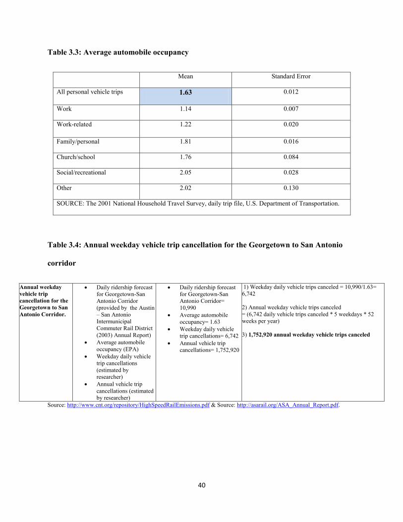
40

Table 3.3: Average automobile occupancy

Mean Standard Error

All personal vehicle trips 1.63 0.012

Work 1.14 0.007

Work-related 1.22 0.020

Family/personal 1.81 0.016

Church/school 1.76 0.084

Social/recreational 2.05 0.028

Other 2.02 0.130

SOURCE: The 2001 National Household Travel Survey, daily trip file, U.S. Department of Transportation.

Table 3.4: Annual weekday vehicle trip cancellation for the Georgetown to San Antonio

corridor

Annual weekday vehicle trip cancellation for the Georgetown to San Antonio Corridor.







Weekday daily vehicle trip cancellations= 6,742


1) Weekday daily vehicle trips canceled = 10,990/1.63= 6,742 2) Annual weekday vehicle trips canceled = (6,742 daily vehicle trips canceled * 5 weekdays * 52 weeks per year) 3) 1,752,920 annual weekday vehicle trips canceled

Source: http://www.cnt.org/repository/HighSpeedRailEmissions.pdf & Source: http://asarail.org/ASA_Annual_Report.pdf.



41

Annual commuter saves in automobile carbon dioxide emissions

By switching to high-speed rail from automobiles as a main source of travel, it is

estimated that the average commuter will save the corridor in the amount of carbon dioxide

(CO2) emitted by automobile annually. In order to calculate the amount of carbon dioxide an

average commuter saves by switching from automobile to high-speed rail travel, a few factors

need to be calculated. The factors needed to complete the calculation are:

The average automobile’s emission of CO2 per passenger mile (0.53 pound) (Table 3.5).

Table 3.5: Average automobile’s emission of CO2 per passenger mile


Also needed, is the average distance between the thirteen train stations located within the

corridor (46.10 miles).

o (In Appendix D, the average distance between thirteen rail stations within the

corridor is calculated by charting out the estimated distances from each train

station to the other twelve connecting train stations. Then next step is to calculate

the average distance of a train station from its connecting twelve stations. Once


42

the average distance for every train station has been charted, the researcher then

calculates the overall average distance of the thirteen train stations from one

another (46.10 miles. The distances computed are not exact and are disputable).

And lastly needed are the number of days commuted per week (five weekdays), and the

number of weeks per year the commuter makes the trip (fifty two weeks in a year) are

needed as well.

The formula used to calculate an individual’s annual automobile emission is modeled

after the same formula used in the Center for Clean Air Policy and Center for

Neighborhood Technology study (shown in Table 3.6).

The formula is: automobile CO2 emission per passenger mile in 2020 (0.53) times

average estimated distance between train stations (46.10) times five days per week times

fifty two weeks per year.

Table 3.6: Annual commuter saves in automobile carbon dioxide emissions








1) Automobile’s emission of CO2 per passenger mile= (0.53 lbs CO2 per passenger mile) * 46.10 miles (average distance between rail stations)* 5 days per week * 52 weeks per year = 10,188.1 lbs CO2 Average commuter saves in automobile carbon dioxide per year


Net annual automobile carbon dioxide emissions saved in the corridor

In this section, a calculation modeled after the same formula used by the Center for Clean

Air Policy and Center for Neighborhood Technology study determines the net automobile

emissions savings within the corridor as a whole. The diverting of individuals from automobile


43

travel to high-speed rail results in annual automobile emissions saved by the entire Georgetown-

San Antonio corridor. The formula shown below in Table 3.7 determines the amount of

automobile emissions saved annually in the Georgetown-San Antonio corridor.

Needed is the average daily miles for riders in the entire corridor, the average

daily miles is computed by multiplying the average distance between rail stations

estimated by the researcher (46.10 miles) by the number of forecasted daily

riders as predicted by the Austin-San Antonio Intermunicipal Commuter Rail

District study (10,990). The result is the predicted daily miles by riders

(492,546.69).

Also needed is the average occupancy of an automobile estimated by the EPA (as

shown above in table 3.2 being 1.63), and the automobile emission rate of CO2

per passenger mile (shown in Table 3.5) (0.53 lbs CO2 per passenger mile).

The next step divides the corridor’s daily miles by riders (492,546.68) by the

average occupancy of an automobile (1.63). That result is then multiplied by the

automobile emissions per passenger mile (0.53). The resulting amount is the

daily savings of automobile emissions for the corridor (160,153.22 lbs of CO2, as

shown in Table 3.7).

To determine the annual amount of savings to the corridor one must simply multiply the

daily amount of CO2 savings for the corridor 160,153.22 by five days a week times fifty two

weeks a year. The 41,639,836.93 lbs CO2 resulting amount is the predicted annual automobile

emissions savings for the Georgetown-San Antonio corridor.

44

Table 3.7: Net Annual Automobile Carbon Dioxide Emissions Saved in the Corridor














Costs

What the individual commuter costs in annual CO2 emission by using high-speed

rail

The following calculation (Table 3.8) is replicated by the formula used in the Center for

Clean Air Policy and Center for Neighborhood Technology 2006 study. The formula determines

the carbon dioxide emission annually by individual commuters by using one of the five high-

speed rail technologies (TGV, ICE, IC-3, Shinkansen, MagLev). Each high-speed rail

technology’s emission rate per passenger mile determines how much an individual commuter is

contributing in annual CO2 emissions by using a selected high-speed rail technology.

To calculate what the individual commuter emits annually by using a high-speed

rail technology a few factors are needed. First is listing the lbs of CO2 per

passenger mile of the five high-speed technologies (Table 3.8).


45

Table 3.8: CO2 emission rate per passenger mile based on five high-speed rail options

High Speed Rail Technology Lbs CO2 Per Passenger Mile

Shinkansen 0.22

TGV 0.15

ICE 0.11

Danish IC-3 0.26

MagLev 0.49


The second step takes each of the high-speed rail technologies’ pounds of CO2 per

passenger mile and multiplies each by the average distance between the thirteen

rail stations that was estimated by the researcher at 46.10 miles (Appendix D).

That amount is then multiplied by five days a week and fifty two weeks a year.

The resulting emission produced is the amount of CO2 an individual commuting

on one of the five high-speed rail technologies produces annually (Table 3.9).

The formula used in this calculation is modeled after the formula used in the

Center for Clean Air Policy and Center for Neighborhood Technology 2006

report, which is shown on the next page in Table 3.9.


46

Table 3.9: What the individual commuter costs in annual CO2 emission depending on high-

speed rail technology selected

What the individual commuter costs in annual CO2 emission depending on high-speed rail technology selected (TGV, Shinkansen, ICE, IC-3,MagLev)




Certain high-speed rail technology’s CO2 emission per passenger mile (TGV= 0.15, Shinkansen= 0.22, ICE= 0.11, IC-3= 0.26, MagLev= 0.49)



1) CO2 per passenger mile (based on high-speed rail technology) TIMES 46.10 miles (average commute between rail stations) TIMES 5 days per week TIMES 52 weeks per year = What the individual commuter produces in annual CO2 emission depending on high-speed rail technology selected TGV= 1,797.9 lbs CO2 annually Shinkansen= 2,636.92 lbs CO2 annually ICE= 1,318.46 lbs CO2 annually IC-3=3,116. 36 lbs CO2 annually MagLev= 5,873.14 lbs CO2 annually


Predicted annual emission of carbon dioxide for each of the five high-speed rail

technologies operating in the Georgetown-San Antonio corridor

The resulting annual cost in high-speed rail operation and emission of CO2 must be

considered when choosing the most efficient technology for operation. By using emission data

on the five high-speed rail technologies provided by the Center for Clean Air Policy and Center

for Neighborhood Technology, the high-speed rail technology option with the lowest annual

carbon dioxide production deems the appropriate choice of high-speed rail technology selected.

Needed to determine the high-speed rail technology with the lowest annual

emission of CO2 are the following factors:

The first factor needed, is the CO2 emission per passenger mile for each of the

five high-speed rail technologies (Table 3.10).


47



Shinkansen 0.22

TGV 0.15

ICE 0.11

Danish IC-3 0.26

MagLev 0.49


The second factor needed is the annual miles by riders predicted for the

Georgetown-San Antonio corridor.

Annual miles by riders are determined by first calculating the daily miles by

riders. Daily miles by riders is calculated by taking the 46.10 miles (average

distance between rail stations within the corridor) and multiplying by the daily

predicted ridership of the corridor (10,990) as predicted by the Austin-San

Antonio Intermunicipal Commuter Rail District study.

The result is 492,546.69 daily miles by riders within the corridor (Table 3.11).

Table 3.11: Average daily miles by riders in the Georgetown-San Antonio corridor

Average Distance 51.70 44.29 43.39 42.89 37.82 36.51 36.41 38.15 42.49 47.25 54.85 58.04 65.45 46.10 Number of daily riders 740 1,110 210 320 580 1,810 980 1,800 490 340 630 1,500 480 10,990 Avg. daily miles driven by riders from each station (Average Distance * Riders) 38,258.00 49,164.46 9,112.38 13,725.54 21,937.38 66,078.92 35,679.54 68,676.92 20,821.23 16,063.69 34,553.08 87,057.69 31,417.85 492,546.69


48

Annual miles by riders is then calculated by simply multiplying the 492,546.69

daily miles, by five week days, and fifty two weeks a year, resulting in

128,062,136.8 annual miles by riders.

Now it is possible to predict the annual emission of CO2 for each of the five high-speed

rail technologies operating in the Georgetown-San Antonio corridor, due to now having the CO2

emission rate per passenger mile based on five high-speed rail options, along with the

128,062,136.8 annual miles by riders.

To calculate the annual emission of CO2 for each of the five high-speed rail

technologies operating within the corridor, the formula used is shown in Table

3.12.

The calculation is completed by multiplying the emissions per passenger mile

for the each high-speed rail technology by the annual miles by riders predicted

for the Georgetown-San Antonio corridor (128,062,136.8).

Table 3.12: Projected high-speed rail annual emissions depending on high-speed rail

technology selected





Certain high-speed rail technology’s CO2 emission per passenger mile. (TGV= 0.15, Shinkansen= 0.22, ICE= 0.11, IC-3= 0.26, MagLev= 0.49).

Daily miles by riders predicted for the Georgetown-San Antonio corridor= 492,546.68.


1) Certain high-speed rail technology’s CO2 emission per passenger mile TIMES 2) Annual miles by riders (128,062,136.8) = Projected high-speed rail annual emissions



49

Human subjects protection

This research poses no risk to human subjects and has been approved by the Institutional

Review Board. The reviewers have determined that your IRB Application Number 2011I7755 is

exempt from IRB review. The project is approved.

50

Chapter 4: RESULTS

Introduction

This chapter presents the findings of the cost benefit analysis conducted based on the

benefit received when commuters switch preferred mode of travel from automobile to high-speed

rail technology on the Interstate 35 corridor. The results of this analysis determine whether travel

by high-speed rail is environmentally beneficial in the reduction of carbon dioxide levels emitted

by automobile travel on interstate 35. This analysis considers the emission data presently

available on high-speed rail technologies along with data on automobile emissions due to a

realistic possibility exists that construction of a high-speed rail system could occur.

United States’ predicted benefits with high-speed rail operation

Current projections supplied by the Center of Clean Air Policy and Center for

Neighborhood Technology show that passengers would take 112 million trips on high-speed rail

in the U.S. in 2025, traveling more than 25 billion passenger miles. These trips would result in

29 million fewer automobile trips and nearly 500,000 fewer flights. The Center of Clean Air

Policy and Center for Neighborhood Technology calculated, as a result of the canceled

automobile trips and flights, a total emission savings of six billion pounds of CO2 per year (2.7

MMTCO2, Million Metric Tons) should all proposed high speed rail systems considered in the

United States be built. These organizations predict the savings from the canceled automobile and

airplane trips to be the primary sources of the emissions savings; together these two modes make

up 80 percent of the estimated emissions savings among all modes of transportation.

51

Cost benefit analysis

The results of the cost benefit analysis determine the amount of benefits received by the

Georgetown-San Antonio corridor. As commuters decide not to use their automobile to make

their daily commute they produce savings in the reduced annual amount of automobile CO2

emitted into the air. The total number of diverted annual passengers can be calculated to

determine the total annual amount of automobile emissions were not emitted into the corridor

due to commuters switching mode of transportation to high-speed rail. The cost represented in

this analysis is the annual amount of carbon dioxide a high-speed rail produces annually,

(Projected high-speed rail annual emissions). The annual emission from high-rail operation is

then subtracted from the annual automobile savings, resulting in a net annual automobile savings

for the corridor. The study then analyses each of the five high-speed rail technologies to

determine the rail technology with the lowest annual contribution of emissions. The next section

discusses the benefits received when commuters switch preferred mode of transportation from

automobile to high-speed rail.

Benefits

Direct Benefits

One benefit that would be a direct result of the proposed high-speed rail system is the

annual number of vehicle trip cancellations in the Georgetown-San Antonio corridor. A second

benefit produced by commuters using high-speed rail is the savings to individual commuter’s

annual amount of automobile emissions due to a change in primary mode of transportation.

Lastly, after calculating the total number of individual trips annually diverted in the Georgetown-

San Antonio corridor, the resulting benefit is the total amount of automobile CO2 emissions

52

savings annually in the corridor; because the total number of automobile trips canceled in the

corridor produce lower annual CO2 emission levels.

Annual Weekday Vehicle Trip Cancellation for the Georgetown to San Antonio Corridor

Vehicle trip cancellation is a benefit of the introduction of high-speed rail, because

emissions savings occur ―when critical masses of passengers switch modes of transportation

causing vehicle trips to be canceled‖ (Center for Clean Air Policy and Center for Neighborhood

Technology 2006, 7). As people leave their vehicles at home or at train stations, vehicle trip

cancellation causes lower annual amounts of carbon dioxide to be emitted into the air. High-

speed rail leads to the canceling of automobile trips and replaces each individual’s emission

output with a combined single source of emission that all the riders on the high-speed rail train

share. Table 4.1 provided by the Austin-San Antonio Intermunicipal Commuter Rail District

study forecasts the predicted weekday ridership for the planned train stations along the


Table 4.1: Average weekday commuter trips diverted in favor of rail for the year (2020)

53

This research uses forecasted ridership data by the Austin-San Antonio Intermunicipal

Commuter Rail District study for the thirteen stops on the Georgetown-San Antonio line. The

formula used by the Center of Clean Air Policy and Center for Neighborhood Technology is

modeled after in this study to predict the vehicle trip cancellation for the corridor in the year

2020. Table 4.1, predicts 10,990 passengers is the daily ridership prediction in the Georgetown-

San Antonio corridor.

Table 4.2: Average automobile occupancy by daily trip purpose

Mean Standard Error

All personal vehicle trips

1.63 0.012

Work 1.14 0.007





Other 2.02 0.130

SOURCE: The 2001 National Household Travel Survey, daily trip file, U.S.

Department of Transportation.

To calculate the number of daily vehicle trip cancellations, the research takes the

10,990 daily diverted passengers and divides by the average automobile

occupancy 1.63 (Table 4.2). The resulting daily number of automobile trips

cancelled in the corridor equals 6,742.

54

Calculating the number of annual automobile trips cancelled by high-speed rail in

the corridor is calculated by following the formula in Table 4.3.

The first step is taking the 6,742 daily automobile trips cancelled and multiplying

by 5 (weekdays), then multiplying by fifty two (weeks in a year).

The resulting number of automobile trips cancelled annually by high-speed rail is

1,752,920.

Table 4.3: Annual weekday vehicle trip cancellation for the Georgetown to San Antonio corridor

Benefits: Name of Components Definition of components Measurement:

Annual weekday vehicle trip cancellation for the Georgetown to San Antonio corridor







A weekday daily vehicle trip cancellations= 6,742


1) Weekday vehicle trips canceled = 10,990/1.63= 6,742 2) Annual weekday vehicle trips canceled = (6,742 daily vehicle trips canceled * 5 weekdays * 52 weeks per year) 3) 1,752,920 annual weekday vehicle trips canceled



55

How much the commuter saves in annual automobile carbon dioxide emissions

By convincing more people to switch to high-speed rail from automobile travel, the

average commuter will save the corridor in the amount of carbon dioxide (CO2) not emitted

annually. Planning and constructing environmentally friendly adjacent housing and development

areas in high-speed rail districts, daily commuters will find high-speed rail a beneficial mode of

transportation. The corridor will benefit by the amount of carbon dioxide an average commuter

saves annually by switching from automobile to high-speed rail. In order to calculate the amount

of carbon dioxide an average commuter saves in annual automobile CO2 emissions, a few factors

are needed:

The 0.53 pounds of CO2 per passenger mile an automobile emits (Table 4.4).

Table 4.4: Summary CO2 Emissions Factors by Mode


The average distance between the thirteen train stations that was computed by the

researcher at 46.10 miles (Table 4.5, exact distance is disputable),


56


The five days commute per week, and the fifty two weeks per year the commuter makes

the trip.

The formula used to calculate an individual’s annual automobile emission has been

replicated in Table 4.6 from the formula used in the Center for Clean Air Policy and Center for

Neighborhood Technology 2006 report.

The first step in calculating the annual commuter’ savings of automobile carbon dioxide

savings, is taking the 0.53 pounds of CO2 per passenger mile emitted from automobiles,

and multiplying by the average distance between train stations along the corridor (46.10

miles),

The result is then multiplied by five (5 weekdays) and lastly multiplied by fifty two (52

weeks in a year).

As the result, the annual commuter within the corridor will be saving 10,188.1 lbs of

automobile CO2 by opting not to use their automobile to travel by.

Average Distance 51.70 44.29 43.39 42.89 37.82 36.51 36.41 38.15 42.49 47.25 54.85 58.04 65.45 46.10 Number of daily riders 740 1,110 210 320 580 1,810 980 1,800 490 340 630 1,500 480 10,990 Avg. daily miles driven by riders from each station (Average Distance * Riders) 38,258.00 49,164.46 9,112.38 13,725.54 21,937.38 66,078.92 35,679.54 68,676.92 20,821.23 16,063.69 34,553.08 87,057.69 31,417.85 492,546.69

57

Table 4.6: Formula to calculate the annual commuter’s savings of automobile carbon

dioxide savings








1) Average automobile’s emission of CO2 per passenger mile (0.53 lbs CO2 per passenger mile) TIMES 46.10 miles (average distance between rail stations) TIMES 5 days per week TIMES 52 weeks per year = 10,188.1 lbs CO2 Average commuter saves in automobile carbon dioxide per year


Net annual automobile carbon dioxide emissions saved in the corridor

In this section a calculation determines the net automobile emissions savings within the

corridor as a whole due to annual automobile trip cancellations. As a result, diverting individuals

from automobile travel to high-speed rail results in net annual automobile emissions savings for

the Georgetown-San Antonio corridor, as shown in Table 4.10.To determine the net annual

automobile emissions savings for the Georgetown-San Antonio corridor, the formula used in the

Center for Clean Air Policy and Center for Neighborhood Technology 2006 report will be

replicated to do so.

To determine the amount of automobile emissions saved annually for the Georgetown-

San Antonio corridor, a few factors are required including the following:

The total daily miles by riders for the corridor (Table 4.7). Total daily miles by

riders is calculated by multiplying the average distance between rail stations

(46.10 miles) times the number of daily riders (10,990).


58

Resulting in 492,546.69 total daily miles by riders (Table 4.7).


Also needed is the 1.63 average occupancy of an automobile (shown in Table 4.8).

Table 4.8: Average automobile occupancy

Mean Standard Error

All personal vehicle trips 1.63 0.012

Work 1.14 0.007





Other 2.02 0.130

SOURCE: The 2001 National Household Travel Survey, daily trip file, U.S.

Department of Transportation.

And lastly needed is the automobile emissions rate per passenger mile (Table 4.9)

Average Distance 51.70 44.29 43.39 42.89 37.82 36.51 36.41 38.15 42.49 47.25 54.85 58.04 65.45 46.10 Number of daily riders 740 1,110 210 320 580 1,810 980 1,800 490 340 630 1,500 480 10,990 Daily miles driven by riders from each station (Average Distance * Riders) 38,258.00 49,164.46 9,112.38 13,725.54 21,937.38 66,078.92 35,679.54 68,676.92 20,821.23 16,063.69 34,553.08 87,057.69 31,417.85 492,546.69

59

Table 4.9: Summary CO2 Emissions Factors by Mode


Now the pieces have been found to determine the net annual emissions savings in the

corridor (as shown in Table 4.10).

The first step is taking the estimated 492,546.68 daily miles by riders (Table 4.7), and

dividing by the average occupancy of an automobile (1.63).

Then multiplying that result by the 0.53 lbs CO2 automobile emissions per passenger

mile.

The resulting amount is the 160,153.22 lbs of CO2 daily savings of automobile emissions

by the corridor (as shown below in Table 4.10).

To determine the annual amount of savings for the corridor, simply multiply the

160,153.22 daily savings of CO2 by five (5 days a week) times fifty two (52 weeks a

year).

The resulting annual automobile emissions savings for the Georgetown-San Antonio

corridor is 41,639,836.93 lbs of CO2 (Table 4.10).


60

Table 4.10: Annual savings of automobile CO2 emissions in corridor














Result

The total amount of automobile emissions saved in the Georgetown-San Antonio corridor

due to the number of total miles of automobile trips canceled and number of diverted automobile

passengers to high-speed rail has the predicted resulting effect of a net annual automobile

savings of 41,639,836.93 lbs of CO2 annually (Table 4.11).


61

Table 4.11: Annual automobile emissions saved by station and corridor

Daily miles by riders from each city

Average Occupancy

Automobile emission per passenger mile (lbs of CO2)

Automobile Emissions Saved Daily

Automobile Emissions Saved Annually

Georgetown 38,258.00 1.63 0.53 12,439.72 3,234,326.63

Round Rock 49,164.46 1.63 0.53 15,985.99 4,156,357.55

McNeil Jct. 9,112.38 1.63 0.53 2,962.92 770,359.88

Research 13,725.54 1.63 0.53 4,462.91 1,160,355.34

US 183 21,937.38 1.63 0.53 7,133.01 1,854,583.80

Austin CBD 66,078.92 1.63 0.53 21,485.78 5,586,304.05

Ben White 35,679.54 1.63 0.53 11,601.32 3,016,343.80

San Marcos 68,676.92 1.63 0.53 22,330.53 5,805,938.65

New Braunfels 20,821.23 1.63 0.53 6,770.09 1,760,224.29

Selma 16,063.69 1.63 0.53 5,223.16 1,358,022.58

SA Airport 34,553.08 1.63 0.53 11,235.05 2,921,112.88

San Antonio

CBD

87,057.69 1.63 0.53 28,307.10 7,359,846.63

Kelly 31,417.85 1.63 0.53 10,215.62 2,656,060.86

Total 492,546.69 1.63 0.53 160,153.22 41,639,836.93

In the next section, this analysis determines annual costs associated with high-speed rail

operation. The first cost identified is the annual amount of CO2 the individual commuter using a

high-speed rail technology emits into the corridor.

62

Costs

What the individual commuter costs in annual CO2 emission by using high-speed

rail

In Table 4.14, the following calculation determines what the individual commuter emits

in carbon dioxide annually using each of the five high-speed rail technologies. The formula used

in the Center for Clean Air Policy and Center for Neighborhood Technology 2006 report will be

replicated to determine what the individual commuter emits in annual CO2 emissions by

traveling by each of the high-speed rail technologies.

To determine what the individual will emit annually by high-speed rail, will depend on a

few factors. The first being what high-speed rail technology is being used, and what the high-

speed rail technology’s emission rate per passenger mile is. As shown in Table 4.12 are the five

high-speed rail technologies looked at in this study and their emission rates per passenger mile.



Shinkansen 0.22

TGV 0.15

ICE 0.11

Danish IC-3 0.26

MagLev 0.49



63

Also needed is the average distance between rail stations (46.10 miles) that was estimated

by the researcher (distance is disputable, shown in Table 4.13).

Table 4.13: average distance between Georgetown-San Antonio corridor rail stations

To calculate what the individual commuter costs in annual CO2 emissions by using the

five high-speed rail technologies, the formula used in the Center for Clean Air Policy and

Center for Neighborhood Technology 2006 report (Table 4.14) is modeled after.

The calculation is completed in taking each of the five high-speed rail technologies’

emission of CO2 per passenger mile, and multiplying each by the average distance

between rail stations in the corridor (46.10 miles),

Georgetown Round Rock

McNeil Jct. Research US 183

Austin CBD

Ben White

San Marcos

New Braunfels Selma

San Antonio Airport

San Antonio

CBD Kelly Total

Georgetown 0 9.7 17.6 20.3 22.7 27.7 32 57 74.9 88.1 101.1 106.1 114.9 672.1

Round Rock 9.7 0 9 9.8 14.1 19.2 23.5 48.4 66.3 79.5 92.5 97.5 106.3 575.8

McNeil Jct. 17.6 9 0 7.7 12.2 16.9 21.6 46.5 64.4 77.6 90.6 95.6 104.4 564.1

Research 20.3 9.8 7.7 0 11.1 15.8 20.4 45.4 63.3 76.5 89.5 94.5 103.3 557.6

US 183 22.7 14.1 12.2 11.1 0 6.5 10.8 35.7 53.6 66.8 79.8 84.8 93.6 491.7

Austin CBD 27.7 19.2 16.9 15.8 6.5 0 5.5 30.4 48.4 61.6 74.6 79.6 88.4 474.6

Ben White 32 23.5 21.6 20.4 10.8 5.5 0 26.5 44.5 57.6 70.7 75.7 84.5 473.3

San Marcos 57 48.4 46.5 45.4 35.7 30.4 26.5 0 19.1 32.3 45.3 50.3 59.1 496 New Braunfels 74.9 66.3 64.4 63.3 53.6 48.4 44.5 19.1 0 15 28 33.1 41.8 552.4

Selma 88.1 79.5 77.6 76.5 66.8 61.6 57.6 32.3 15 0 13.4 18.5 27.3 614.2 San Antonio Airport 101.1 92.5 90.6 89.5 79.8 74.6 70.7 45.3 28 13.4 0 9.5 18 713 San Antonio CBD 106.1 97.5 95.6 94.5 84.8 79.6 75.7 50.3 33.1 18.5 9.5 0 9.3 754.5

Kelly 114.9 106.3 104.4 103.3 93.6 88.4 84.5 59.1 41.8 27.3 18 9.3 0 850.9 Average Distance 51.70 44.29 43.39 42.89 37.82 36.51 36.41 38.15 42.49 47.25 54.85 58.04 65.45 46.10

64

The result from each of the five rail technologies is then multiply by five (5 days a week)

and fifty two (52 weeks a year) that the commute is made.

Table 4.14: Commuter’s annual emission footprint by using a high-speed rail technology

What the individual commuter costs in annual CO2 emission depending on high-speed rail technology selected. (TGV, Shinkansen, ICE, IC-3,MagLev)

Certain high-speed rail technology’s CO2 emissions per passenger mile

Average distance between rail stations


Certain high-speed rail technology’s CO2 emissions per passenger mile. (TGV= 0.15, Shinkansen= 0.22, ICE= 0.11, IC-3= 0.26, MagLev= 0.49)



1) CO2 per passenger mile (based on high-speed rail technology) * 46.10 miles (average commute between rail stations) * 5 days per week * 52 weeks per year = What the individual commuter costs in annual CO2 emission depending on high-speed rail technology selected


The resulting annual CO2 emission for a commuter using each of the five high-

speed technologies in the Georgetown-San Antonio corridor is shown below in

Table 4.15.

Table 4.15: Annual emission for a commuter using each of the five high-speed rail

technologies within the Georgetown-San Antonio corridor

High Speed Rail Technology

Lbs CO2 Per Passenger Mile

Average distance between rail

stations (miles)

Five weekdays

Fifty two weeks a year

Annual CO2 emission for an individual

commuter using high-speed rail in the Georgetown-San

Antonio Corridor (Lbs of CO2)

Shinkansen 0.22 X 46.10 X 5 X 52 = 2,636.92

TGV 0.15 X 46.10 X 5 X 52 = 1,797.9

ICE 0.11 X 46.10 X 5 X 52 = 1,318.46

Danish IC-3 0.26 X 46.10 X 5 X 52 = 3,116.36

MagLev 0.49 X 46.10 X 5 X 52 = 5,873.14


65

The results show that the ICE high-speed rail technology produces the lowest annual amount of

CO2 emission per individual rider. In the next section the research will determine out of the five

high-speed rail technologies designated for operation in the corridor, of which produces the

lowest amount of annual CO2 emissions due to each of the five technologies operation.

Predicted annual emission of carbon dioxide for each of the five high-speed rail

technologies running in the Georgetown to San Antonio corridor

An annual savings of 41,639,836.93 lbs of automobile carbon dioxide (CO2) emissions

means the air quality and environment would benefit from a high-speed rail system. But, the

resulting annual cost by high-speed rail operation and emission of CO2 must be considered when

choosing the most efficient technology for operation. Emission data on the five high-speed rail

technologies provided by the Center for Clean Air Policy and Center for Neighborhood

Technology, will determine the high-speed rail technology option with the lowest carbon dioxide

production annually and the appropriate choice of high-speed rail technology to use in the


The formula used to determine each high-speed rail annual emissions appears in

Table 4.18, as replicated by the formula used in the Center for Clean Air Policy

and Center for Neighborhood Technology report.

Criteria needed for calculation include:

o The emissions per passenger mile for the each high-speed rail technology

(Table 4.16) ,

66

Table 4.16: Five high-speed rail technologies’ CO2 lbs per passenger mile

High Speed-Rail Technology

Lbs CO2 Per Passenger

Mile Shinkansen 0.22

TGV 0.15

ICE 0.11

Danish IC-3 0.26

MagLev 0.49


o And the annual miles by riders forecasted by the researcher for the Georgetown-

San Antonio corridor :

(492,546.68 daily miles by riders (Table 4.17) predicted for the

Georgetown-San Antonio corridor times

five days a week times

fifty two weeks a year= 128,062,136.8 annual miles by riders).


Average Distance 51.70 44.29 43.39 42.89 37.82 36.51 36.41 38.15 42.49 47.25 54.85 58.04 65.45 46.10 Number of daily riders 740 1,110 210 320 580 1,810 980 1,800 490 340 630 1,500 480 10,990 Daily miles driven by riders from each station (Average Distance * Riders) 38,258.00 49,164.46 9,112.38 13,725.54 21,937.38 66,078.92 35,679.54 68,676.92 20,821.23 16,063.69 34,553.08 87,057.69 31,417.85 492,546.69


67

Now having the parts needed to complete the formula replicated after the formula used in

the Center for Clean Air Policy and Center for Neighborhood Technology report (Table 4.18).

Table 4.18: Formula to determine the projected high speed rail technology’s annual

emissions footprint



Daily miles by riders predicted for the Georgetown-San Antonio corridor (estimated by researcher)

Annual miles by riders predicted for the Georgetown-San Antonio corridor (estimated by researcher)

Certain high-speed rail technology’s CO2 emissions per passenger mile (TGV= 0.15, Shinkansen= 0.22, ICE= 0.11, IC-3= 0.26, MagLev= 0.49)

Daily miles by riders predicted for the Georgetown-San Antonio corridor= 492,546.68


1) Certain high-speed rail technology’s CO2 emissions per passenger mile TIMES 2) Annual miles by riders predicted for the Georgetown-San Antonio corridor (128,062,136.8) = Projected high-speed rail annual emissions

To determine the annual emission of CO2 for each of the five high-speed rail technologies

operating in the Georgetown-San Antonio corridor, is simply done by taking each of the

five high-speed rail technologies’ lbs of CO2 per passenger mile and multiply each by the

(128,062,136.8) annual miles by riders estimated in the corridor.

68

Table 4.19: Five high-speed rail technologies’ annual emission footprint for Georgetown-

San Antonio Corridor



Annual miles by riders for the

Georgetown-San Antonio corridor

Annual Emission footprint for

Georgetown-San Antonio Corridor (Lbs of

CO2 per year)

Shinkansen 0.22 X 128,062,136.8 = 28,173,670.10

TGV 0.15 X 128,062,136.8 = 19,209,320.52

ICE 0.11 X 128,062,136.8 = 14,086,835.05

Danish IC-3 0.26 X 128,062,136.8 = 33,296,155.57

MagLev 0.49 X 128,062,136.8 = 62,750,447.03

This analysis determines in Table 4.19 the high-speed rail technology to have the least

effect on the net annual automobile emissions savings of CO2 in the Georgetown-San Antonio

corridor by producing the lowest amount of CO2 annually. As shown above in Table 4.19, after

calculating the five high-speed rail trains’ projected high-speed rail annual emissions , this

analysis indicates out of the five high-speed rail technologies, the German Intercity Express

(ICE) train would provide the best benefit. The ICE high-speed rail technology has the lowest

CO2 emission per passenger mile during operation (0.11), as well as the smallest annual emission

footprint (14,086,835.05 lbs of CO2 per year). The next section determines the effect that each of

the five high-speed rail technologies’ annual emissions of CO2 has on the net annual automobile

emissions savings (41,639,836.93lbs of CO2) projected for the Georgetown- San Antonio

corridor.

69

Model Results

Resulting net annual emissions savings of CO2 in Georgetown-San Antonio

corridor due to a high-speed rail operation

To calculate the effect that each high-speed rail technology’s annual emission of CO2

would have on the saved net annual automobile emissions for the Georgetown- San Antonio

corridor, the following equation (Table 4.20) applies.

Table 4.20: Net annual emissions savings for Georgetown-San Antonio corridor

To determine the best high-speed rail option to use in the Georgetown-San Antonio

corridor is done by taking the 41,639,836.93lbs of CO2 net annual automobile emissions savings

in the corridor (shown on the next page in Table 4.21) ,

Net annual emissions savings=

41,639,836.93lbs of CO2 automobile annual emissions savings (minus) Projected high-speed rail technology annual emission.

70

Table 4.21: Annual automobile emissions saved by station and corridor

Daily miles by riders from each city

Average Occupancy

Automobile emission per passenger mile (lbs of CO2)

Automobile Emissions Saved Daily

Automobile Emissions Saved Annually

Georgetown 38,258.00 1.63 0.53 12,439.72 3,234,326.63

Round Rock 49,164.46 1.63 0.53 15,985.99 4,156,357.55

McNeil Jct. 9,112.38 1.63 0.53 2,962.92 770,359.88

Research 13,725.54 1.63 0.53 4,462.91 1,160,355.34

US 183 21,937.38 1.63 0.53 7,133.01 1,854,583.80

Austin CBD 66,078.92 1.63 0.53 21,485.78 5,586,304.05

Ben White 35,679.54 1.63 0.53 11,601.32 3,016,343.80

San Marcos 68,676.92 1.63 0.53 22,330.53 5,805,938.65

New Braunfels 20,821.23 1.63 0.53 6,770.09 1,760,224.29

Selma 16,063.69 1.63 0.53 5,223.16 1,358,022.58

SA Airport 34,553.08 1.63 0.53 11,235.05 2,921,112.88

San Antonio

CBD

87,057.69 1.63 0.53 28,307.10 7,359,846.63

Kelly 31,417.85 1.63 0.53 10,215.62 2,656,060.86

Total 492,546.69 1.63 0.53 160,153.22 41,639,836.93

and subtracting from the 41,639,836.93lbs CO2 automobile emissions saved, each of the five

high-speed rail technologies’ annual emission produced (shown below in Table 4.22).

71

Table 4.22: Five high-speed rail technologies’ annual emission footprint for Georgetown-

San Antonio Corridor



Annual miles by riders for the

Georgetown-San Antonio corridor

Annual Emission footprint for

Georgetown-San Antonio Corridor (Lbs of

CO2 per year)

Shinkansen 0.22 X 128,062,136.8 = 28,173,670.10

TGV 0.15 X 128,062,136.8 = 19,209,320.52

ICE 0.11 X 128,062,136.8 = 14,086,835.05

Danish IC-3 0.26 X 128,062,136.8 = 33,296,155.57

MagLev 0.49 X 128,062,136.8 = 62,750,447.03

After completing the formula in Table 4.22 for each of the five high-speed rail

technologies, the results are shown in Table 4.23 to determine which of the five high-speed rail

technologies produces the greatest benefit by having the lowest cost in its own operation and

annual emission.

Table 4.23: Total annual net emissions savings by high-speed rail technology

Shinkansen TGV ICE Danish IC-3 MagLev

Automobile emissions saved

annually

41,639,836.93 41,639,836.93 41,639,836.93 41,639,836.93 41,639,836.93 Projected high-speed rail annual emission 28,173,670.10 19,209,320.52 14,086,835.05 33,296,155.57 62,750,447.03 Net annual emissions

savings by rail technology 13,466,166.83 22,430,516.41 27,553,001.88 8,343,681.36 -21,110,610.10

72

This study predicts that an annual net automobile emissions savings of 27,553,001.88 lbs

of carbon dioxide (CO2) in the Georgetown-San Antonio corridor because German ICE high-

speed rail technology produces the lowest projected annual emission cost of the five high-speed

rail technologies (14,086,835.05 lbs of CO2). Thus, the ICE high-speed rail technology would be

the appropriate choice for the Georgetown-San Antonio corridor.

Conclusion

This chapter discusses the costs and benefits as a result of commuters switching from

automobile technology to one the five high-speed rail technologies in the Georgetown-San

Antonio corridor. Each high-speed rail technology was evaluated to determine which of the five

high-speed rail technologies’ annual net emission impacts would benefit the Georgetown- San

Antonio corridor the greatest by diverting automobile commuters to the railway producing an

annual carbon dioxide emission during operation not detrimental to the net automobile emissions

saved. In estimating each of the five high-speed rail technologies’ annual net emission impacts,

the resulting carbon dioxide (CO2) saved from automobile commuters switching to the ICE high-

speed rail would result in an annual emissions savings of 27,553,001.88 lbs of carbon dioxide

(CO2). Though the German Intercity Express (ICE) high speed rail system produces the best

results in terms of net emissions saved annually, planners should also take into consideration all

costs and benefits of a high-speed rail systems’ implementation and decide the capital project’s

viability accordingly. The following chapter discusses the conclusions of the analysis.

73

Chapter 5: CONCLUSION

Introduction

This chapter provides a summary of the cost-benefit analysis performed on a proposed

high-speed rail transportation system in Central Texas. This chapter recommends the German

Intercity Express (ICE) high-speed rail technology as the train system that will provide the

largest benefit to the region while causing the smallest annual emission thereby minimally

impacting the net annual automobile emissions savings in the corridor.

Summary

This research project began by discussing the ongoing problems caused by traffic

congestion along the Interstate 35 corridor, and how the State of Texas has tried to remodel its

roadways to ease the burden on its highway transportation system, with little effect. The vision

of constructing a high-speed rail system that breezes through and connecting the state’s major

cities exhausted by overcrowding and traffic congestion has been a goal of the state’s public

administrators as well as anyone who has travelled down Interstate 35 at rush hour. All the

benefits associated with high-speed rail systems in operation worldwide are possible in Texas, as

well. Chapter two researched, reviewed, and examined the available literature on high-speed rail

transportation systems around the world and the costs and benefits associated with their high-

speed networks. The chapter also examines from the beginning, United States President Barack

Obama’s vision to incorporate a high-speed rail system into the nation’s already overburdened

transportation system. The literature review begins the cost-benefit analysis by identifying the

environmental costs and benefits that would result in the operation of a high-speed network;

74

specifically, the effect of the greenhouse gas carbon dioxide (CO2) and the gases’ emission rates

based on available high-speed rail technologies.

Chapter three, the Methodology chapter, reviews why a cost benefit analysis was an

appropriate method to address the research question. The purpose of this paper is to conduct a

cost-benefit analysis focusing on a high-speed rail system between Georgetown and San

Antonio, and to determine if this mode of transportation is a viable investment in reducing the

annual amount of automobile carbon dioxide emissions. The data used for this study derived

from existing published studies utilizing modeling shows high-speed rail, if built as planned, will

generate substantial environmental savings. Benefits occur when annual automobile trips are

canceled and by annual mileage not driven in the corridor due to diverting automobile passengers

onto the railway. The resulting annual savings occurs in the amount of automobile CO2 not

emitted into the air for that year. While there is a savings in the annual amount of automobile

CO2 not being emitted into the air, high-speed rail itself produces a cost in the annual amount of

CO2 it produces due to its operation. The research evaluates five high-speed rail technologies to

determine which of the five is the least detrimental to the Georgetown-San Antonio corridor’s

annual amount of automobile savings, i.e., which is the best option by producing the lowest

amount of annual emission of CO2. The best option is the high-speed rail technology with the

lowest annual emission of CO2; that is the least detrimental to the net annual automobile

emissions saved in the corridor. The data for the five high-speed rail technology emission rates,

average automobile emission rate, and ridership and diversion rates, came from existing data

published by The Center for Neighborhood Technology (CNT), the Center for Clear Air Policy

(CCAP), Environmental Protection Agency (EPA), and the Austin- San Antonio Intermunicipal

Commuter Rail District Study

75

Chapter four, the Results chapter, shows the direct benefits and costs associated with

implementation of a high-speed rail network in the Georgetown-San Antonio corridor. The

results show the direct benefits in the form of annual vehicle trip cancellations, how much the

average commuter saves in carbon dioxide emissions by switching to high-speed rail, and net

annual automobile emissions saved in the corridor. The only cost considered is the operation and

annual running of the selected high-speed rail technology. The research analyzed each high-

speed rail technology to determine which of the five high-speed rail technologies’ net emission

impacts would benefit the Georgetown- San Antonio corridor the greatest by diverting

automobile commuters onto its rails and producing an annual carbon dioxide level not

detrimental to the automobile emissions saved. This research concludes that the German Intercity

Express (ICE) high-speed rail technology produces the best results (as shown in Table 4.23) in

the lowest amount of emission per passenger mile (0.11 lbs of CO2), the lowest cost in annual

production of carbon dioxide (CO2) due to its operation (14,086,835.05 lbs of CO2), and most

importantly, the highest amount of annual net emission savings totaled at 27,553,001.88 lbs of

carbon dioxide (CO2) annually. The results are based on current projections of available data at

this time. If the project actually begins construction later than year 2020, a new forecast should

be done taking in consideration changes in technology and data available.

Recommendations

The results of this cost-benefit analysis forecast the annual emissions savings produced

by the five high-speed rail technologies for the year 2020. By following the methodology used in

this research, the State of Texas, as well as other states and nations can model research in similar

fashion to determine whether high-speed rail will benefit local annual carbon dioxide levels. This

76

study along with the Center for Neighborhood Technology (CNT) and Center for Clean Air

Policy (CCAP) recommends further research to better understand the potential impact of high

speed rail’s costs and benefits. In areas with cleaner than average electricity generation

production derived from other natural resources, such as wind, solar, or hydroelectric generated

electricity high-speed rail may be much more environmentally sound and the preferred choice.

Improved and updated energy and emissions data on past and emerging high-speed rail

technologies should constantly be reviewed to improve the understanding of the energy use and

emissions impact of intercity travel by high-speed rail technologies. The most direct way to

impact the emissions associated with high-speed rail is to improve the efficiency of the trains. As

described in the literature review, more efficient diesel locomotive engines and other

improvements, such as regenerative braking, are being developed to improve high-speed rail

efficiency. Local, state, and federal government can use cost benefit analysis to determine

whether a project benefits the public. The same can be said for the environment. Officials may

also use cost benefit analysis to determine the best transportation options based on environmental

impact.

77

Bibliography

Akerman, Jonas. 2011. The role of high-speed rail in mitigating climate change- the Swedish case europabanan from a life cycle perspective. Transportation Research Part D: Transport and Environment. 16 (3): 208-217.

Alvarez, Alberto G. 2010. Energy consumption and emissions of high-speed trains. Journal of

the Transportation Research Board 2159: 27-35. Austin – San Antonio Intermunicipal Commuter Rail District (2003) Annual Report, 1-

Appendix C-7-9. http://asarail.org/ASA_Annual_Report.pdf. Babcock, Lace, Jeffery Barg, Amy Berknopf, Cassidy Boulan, Jeff Bumgardner, Trinity Buch,

Ted Clement, Diana Cornely, Yirui Huang, Lisa Jacobson, Kate Keller, Zlata Kobzantsev, Erika Lindsey, Reuben MacMartin, Colin McLean, Danny O’Shaughnessy, Bryan Rodda, and Selina Zapata. 2010. Making high-speed rail work in the northeast megaregion: Shaping the future through strategic transportation investments. University of Pennsylvania: School of design.

Billitteri, Thomas. 2009. High-speed trains: does the United States need supertrains?

Congressional Quarterly 19 (17): 397-420. Bingham, Richard. 1988. Evaluation in practice: A methodological approach. Longman Group

United Kingdom. Bliss, Jillian. 2011. Inter-urban rail making stops in San Marcos near campus. The University

Star.

Bombardier. 2001. Mobility for tomorrow. Bombardier transportation in Hungary. http://www.bombardier.com/files/en/supporting_docs/BT_Hungary.pdf

California Office of Traffic Safety. 2008. California traffic safety report card. State of

California, Ca: Safety Report Card: 1-1. Campos, Javier, and Gines de Rus. 2009. Some stylized facts about high-speed rail: a review of

HSR experiences around the world. Transport Policy 16 (1): 19-28. CALPIRG Education Fund. 2010. Next Stop: California, The Benefits of High-Speed Rail

Around the World and What’s in Store for California. Sacramento, CA: U.S. PIRG Education Fund, CALPIRG Education Fund.


http://www.bombardier.com/files/en/supporting_docs/BT_Hungary.pdf

78

Chen, Xueming, and Ming Zhang. 2010. High-speed rail project development processes in the United States and China. Journal of the Transportation Research Board.2159: 9-17.

Community of European Railway and Infrastructure Companies and International Union of

Railways. 2008. Rail Transport and Environment: Facts and Figures. HCB Publishing Ltd.

Drake A, A.M. Bassi, E.L. Tennyson, and H.R. Herren. 2009. Evaluating the creation of a

parallel non-oil transportation system in an oil constrained future. Transport Policy Journal 1265 (9): 1-18.

Fender, Keith (August 2010). "TGV: High Speed Hero". Trains Magazine (8): 70. Glaeser, Edward. 2009. How big are the environmental benefits of high speed rail? New York

Times. Givoni, Moshe, Ross Capon, George Haikalis, David Simpson, and Elaine King. 2010. Current

research and development in intercity rail passenger systems. Transportation Research Board 16: 2-15.

Glave, James, and Rachel Swaby. 2010. Superfast bullet trains are finally coming to the U.S.

Wired Magazine. 1-30. Gutierrez, Javier, Rafael Gonzalez, and Gabriel Gomez. 1996. The european high-speed train

network: predicted effects on accessibility patterns. Journal of Transport Geography 4(4): 227-238.

Hosansky, David. 199. Traffic congestion: Is the United States facing permanent gridlock?

Congressional Quarterly 9(32): 729-752. Jorgensen, M W, and Sc Sorenson. 1997. Estimating emissions from railway traffic.

International Journal of Vehicle Design. Inderscience. http://inderscience.metapress.com/index/j3a7kd81au3q5xcw.pdf.

Kao, Tsung C., Yung-Cheng Lai, and Mei-Cheng Shih. 2010. Privatization versus public works

for high-speed rail projects. Journal of the Transportation Research Board 2159: 18-26. Langer, Gary. 2005. Poll: Traffic in the United States: A Look Under the Hood of a

Nation on Wheels. ABC News. http://abcnews.go.com/Technology/Traffic/story?id=485098&page=1

http://inderscience.metapress.com/index/j3a7kd81au3q5xcw.pdf

http://abcnews.go.com/Technology/Traffic/story?id=485098&page=1

79

Lever, James H. 1998.Technical Assessment of Maglev System Concepts Final Report by the Government Maglev System Assessment Team. U.S. Army Corps of Engineers, Cold Regions Research and Engineering Laboratory. http://www.crrel.usace.army.mil/techpub/CRREL_Reports/html_files/SR98_12.html

Levinson, David, Jean Michel Mathieu, and Adib Kanafani. 1997. The full cost of high-speed

rail: an engineering approach. The Annals of Regional Science 31: 189-215. Linneman, Peter, and Saiz, Albert. 2006. Forecasting 2020 U.S. County and MSA populations.

University of Pennsylvania. Masson, Sophie, and Romain Petiot. 2009. Can the high speed rain reinforce tourism

attractiveness? The case of the high speed rail between Perpignan (France) and Barcelona (Spain). Technovation 29: 611-617.

Pazour, Jennifer A., Meller, Russel D, and Pohl, Letitia M. 2010. A model to design a national

high-speed rail network for freight distribution. Transportation Research Part A: Policy and Practice. (3) 44: 119- 135

Peter Jehle, René Naumann, Rainer Schach (2006). Transrapid und Rad-Schiene- Hochgeschwindigkeitsbahn: Ein gesamtheitlicher Systemvergleich. Springer. p. 20.

Peterman, D., Frittelli, J. and Mallett, W. 2009. High-speed rail (HSR) in the Unites States.

Congressional Research Service (CRS). Report for Congress. December 8. Prest, A. R. and Turvey, R. 1965. Cost-benefit analysis: a survey. The Economic Journal,

300(75), 683-735.

Rail, High Speed. 2006. High Speed Rail and Greenhouse Gas Emissions in the U.S. Communication. http://www.cnt.org/repository/HighSpeedRailEmissions.pdf.

Romero, Phillip J. 2008. Unlocking the gridlock in Los Angeles County’s transportation system:

the local economic benefits of high-speed rail. Los Angeles: California State University. Salameh, Mamdough G. 2003. The new frontiers for the United States energy security in the 21st

century. Applied Energy. 76 (1-3): 135-144. Schrank, David, Tim Lomax, and Shawn Turner. 2010. TTI’s 2010

Urban Mobility Report. College Station, TX: Texas Transportation Institute, A&M University.

http://www.crrel.usace.army.mil/techpub/CRREL_Reports/html_files/SR98_12.html


80

Shields, Patricia M. 1998. Pragmatism as philosophy of science: A tool for public administration. Research in Public Administration 4: 195-225. http://ecommons.txstate.edu/polsfacp/33/

Shields, P. and H. Tajalli 2006. Intermediate theory: The missing link in successful student

scholarship" Journal of Public Affairs Education 12 (3): 313-334. http://ecommons.txstate.edu/polsfacp/39/

Smith, Roderick A. (2003). "The Japanese Shinkansen". The Journal of Transport History

(Imperial College, London) 24/2: 222–236

Tanaka, Yuki, and Masakazu Monji. 2010. Application of post assessment of kyushu shinkansen

network to proposed U.S. high-speed railway project. Journal of the Transportation Research Board 0361-1981 (2159): 1-8.

Thompson, Louis. S. 1994. High speed rail (HSR) in the United States—why isn’t there more?

Japan Railway and Transport Review 3: 32–39.

The United States conference of Mayors. 2010. The economic impacts of high-speed rail on cities and their metropolitan areas. Washington, DC: Economic Development Group, Inc., Siemens Inc.

U.S. Department of Transportation. Office of Public Affairs. 2009. President Obama, Vice

President Biden, Secretary LaHood Call for U.S. High-Speed Passenger Trains. White House, Washington, DC. http://www.whitehouse.gov/the-press-office/2011/02/08/vice-president-biden-announces-six-year-plan-build-national-high-speed-r

U.S. Department of Transportation. 2010. National rail plan moving forward: a progress report

of factors that demonstrate the importance of efficient and effective rail infrastructure to the nation’s economy. Washington, DC: Federal Railroad Administration.

U.S. Department of Transportation. 1997. High-speed ground transportation for America:

report examining the economics of binging high-speed ground transportation (HSGT) to well-populated groups of cities throughout the United States. Washington, DC: Federal Railroad Administration.

U.S. Government Accountability Office. 2009. High Speed Passenger Rail: Future Development

Will Depend on Addressing Financial and Other Challenges and Establishing a Clear Federal Role. Government Accountability Office. pp. 64–68.

http://ecommons.txstate.edu/polsfacp/33/

http://ecommons.txstate.edu/polsfacp/39/

http://www.whitehouse.gov/the-press-office/2011/02/08/vice-president-biden-announces-six-year-plan-build-national-high-speed-r

http://www.whitehouse.gov/the-press-office/2011/02/08/vice-president-biden-announces-six-year-plan-build-national-high-speed-r

81

U.S. Office of the Press Secretary. 2009. Remarks by the President and the Vice President on a

vision for high-speed rail in America. White House: 1-4. Urena, Jose, Philippe Menerault, and Maddi Garmendia. 2009. The high-speed rail challenge for

big intermediate cities: a national, regional and local perspective. Cities. 26: 266-279. Vuchich, Vukan and Jeffery Casello. 2002. An evaluation of maglev technology and its

comparison with high speed rail. Transportation Quarterly 56 (2): 33-49. Worsnop, Richard. 1993. High-speed rail: does the high cost outweigh the anticipated benefits?

Congressional Quarterly 3 (14): 1-27. Yan Luguang. Technology of the High-Speed Magnetic Suspension Vehicle and Its Strategic

Position in China’s Passenger Transport. Science and Technology Review, No. 8, Aug. 1999.

82

Appendix A

Map of Proposed Lone Star Commuter Rail

83

Appendix B

Map of United States’ petroleum imports

84

Appendix C

United States Traffic fatalities rates from 1990-2009 per 100 million miles traveled

Alabama 1,121 996 1,154 1,148 1,207 1,110 969 848 2.6 1.8 2.0 1.9 2.0 1.8 1.6 1.5

Alaska 98 106 101 73 74 82 62 64 2.5 2.3 2.0 1.5 1.5 1.6 1.3 1.3

Arizona 869 1,036 1,151 1,179 1,293 1,071 938 807 2.5 2.1 2.0 2.0 2.1 1.7 1.5 1.3

Arkansas 604 652 703 654 665 649 600 585 2.9 2.2 2.2 2.1 2.0 2.0 1.8 1.8

California 5,192 3,753 4,120 4,333 4,240 3,995 3,434 3,081 2.0 1.2 1.3 1.3 1.3 1.2 1.1 1.0

Colorado 544 681 667 606 535 554 548 465 2.0 1.6 1.5 1.3 1.1 1.1 1.2 1.0

Connecticut 385 341 294 278 311 296 302 223 1.5 1.1 0.9 0.9 1.0 0.9 1.0 0.7

Delaware 138 123 134 133 148 117 121 116 2.1 1.5 1.4 1.4 1.6 1.2 1.4 1.3

District of Columbia 48 48 43 48 37 44 34 29 1.4 1.4 1.2 1.3 1.0 1.2 0.9 0.8

Florida 2,891 2,999 3,244 3,518 3,357 3,213 2,980 2,558 2.6 2.0 1.7 1.8 1.7 1.6 1.5 1.3

Georgia 1,562 1,541 1,634 1,729 1,693 1,641 1,495 1,284 2.2 1.5 1.4 1.5 1.5 1.5 1.4 1.2

Hawaii 177 132 142 140 161 138 107 109 2.2 1.5 1.5 1.4 1.6 1.3 1.0 1.1

Idaho 244 276 260 275 267 252 232 226 2.5 2.0 1.8 1.9 1.8 1.6 1.5 1.5

Illinois 1,589 1,418 1,355 1,363 1,254 1,248 1,043 911 1.9 1.4 1.2 1.3 1.2 1.2 1.0 0.9

Indiana 1,049 886 947 938 902 898 820 693 2.0 1.3 1.3 1.3 1.3 1.2 1.1 0.9

Iowa 465 445 388 450 439 446 412 372 2.0 1.5 1.2 1.5 1.4 1.4 1.3 1.2

Kansas 444 461 459 428 468 416 384 386 1.9 1.6 1.6 1.4 1.6 1.4 1.3 1.3

Kentucky 849 820 964 985 913 864 825 791 2.5 1.8 2.0 2.1 1.9 1.8 1.7 1.7

Louisiana 959 938 927 963 987 993 916 821 2.5 2.3 2.1 2.1 2.2 2.2 2.0 1.8

Maine 213 169 194 169 188 183 155 159 1.8 1.2 1.3 1.1 1.3 1.2 1.1 1.1

Maryland 707 588 643 614 652 614 591 547 1.7 1.2 1.2 1.1 1.2 1.1 1.1 1.0

Massachusetts 605 433 476 441 429 434 364 334 1.3 0.8 0.9 0.8 0.8 0.8 0.7 0.6

Michigan 1,571 1,382 1,159 1,129 1,086 1,087 980 871 1.9 1.4 1.1 1.1 1.0 1.0 1.0 0.9

Minnesota 566 625 567 559 494 510 455 421 1.5 1.2 1.0 1.0 0.9 0.9 0.8 0.7

Mississippi 750 949 900 931 911 884 783 700 3.1 2.7 2.3 2.3 2.2 2.0 1.8 1.7

Missouri 1,097 1,157 1,130 1,257 1,096 992 960 878 2.2 1.7 1.6 1.8 1.6 1.4 1.4 1.3

Montana 212 237 229 251 264 277 229 221 2.5 2.4 2.0 2.3 2.3 2.5 2.1 2.0

Nebraska 262 276 254 276 269 256 208 223 1.9 1.5 1.3 1.4 1.4 1.3 1.1 1.2

Nevada 343 323 395 427 431 373 324 243 3.4 1.8 2.0 2.1 2.0 1.7 1.6 1.2

New Hampshire 158 126 171 166 127 129 138 110 1.6 1.0 1.3 1.2 0.9 1.0 1.1 0.9

New Jersey 886 731 723 747 771 724 590 583 1.5 1.1 1.0 1.0 1.0 1.0 0.8 0.8

New Mexico 499 432 521 488 484 413 366 361 3.1 1.9 2.2 2.0 1.9 1.5 1.4 1.4

New York 2,217 1,460 1,495 1,434 1,454 1,332 1,238 1,156 2.1 1.1 1.1 1.0 1.0 1.0 0.9 0.9

North Carolina 1,385 1,557 1,573 1,547 1,554 1,676 1,428 1,314 2.2 1.7 1.6 1.5 1.5 1.6 1.4 1.3

North Dakota 112 86 100 123 111 111 104 140 1.9 1.2 1.3 1.6 1.4 1.4 1.3 1.7

Ohio 1,638 1,366 1,286 1,321 1,238 1,255 1,191 1,021 1.8 1.3 1.2 1.2 1.1 1.1 1.1 0.9

Oklahoma 641 650 774 803 765 766 750 738 1.9 1.5 1.7 1.7 1.6 1.6 1.6 1.6

Oregon 579 451 456 487 478 455 416 377 2.2 1.3 1.3 1.4 1.4 1.3 1.2 1.1

Pennsylvania 1,646 1,520 1,490 1,616 1,525 1,491 1,468 1,256 1.9 1.5 1.4 1.5 1.4 1.4 1.4 1.2

Rhode Island 84 80 83 87 81 69 65 83 1.1 1.0 1.0 1.1 1.0 0.8 0.8 1.0

South Carolina 979 1,065 1,046 1,094 1,045 1,077 921 894 2.8 2.3 2.1 2.2 2.1 2.1 1.9 1.8

South Dakota 153 173 197 186 191 146 121 131 2.2 2.1 2.2 2.2 2.1 1.6 1.4 1.4

Tennessee 1,177 1,307 1,339 1,270 1,284 1,211 1,043 989 2.5 2.0 1.9 1.8 1.8 1.7 1.5 1.4

Texas 3,250 3,779 3,699 3,536 3,531 3,466 3,476 3,071 2.1 1.7 1.6 1.5 1.5 1.4 1.5 1.3

Utah 272 373 296 282 287 299 276 244 1.9 1.7 1.2 1.1 1.1 1.1 1.1 0.9

Vermont 90 76 98 73 87 66 73 74 1.5 1.1 1.3 1.0 1.1 0.9 1.0 1.0

Virginia 1,079 929 922 947 962 1,027 825 757 1.8 1.2 1.2 1.2 1.2 1.3 1.0 0.9

Washington 825 631 567 649 633 571 521 492 1.8 1.2 1.0 1.2 1.1 1.0 0.9 0.9

West Virginia 481 411 410 374 410 432 378 356 3.1 2.1 2.0 1.8 2.0 2.1 1.8 1.8

Wisconsin 769 799 792 815 724 756 605 561 1.7 1.4 1.3 1.4 1.2 1.3 1.1 1.0

Wyoming 125 152 164 170 195 150 159 134 2.1 1.9 1.8 1.9 2.1 1.4 1.7 1.4

FOOTNOTES

For more information:

http://www.nhtsa.dot.gov/portal/site/nhtsa/menuitem.a0bd5d5a23d09ec24ec86e10dba046a0/

http://www-nrd.nhtsa.dot.gov/CATS/index.aspx

Internet release date: 09/30/2011

Source: U.S. National Highway Traffic Safety Administration, Traffic Safety Facts, annual.

\1 Deaths per 100 million vehicle miles traveled.

85

Appendix D

Average distance traveled between destinations, Number of daily riders, Average daily miles driven by riders from each station, Daily number of car trip cancelled, Average auto occupancy

Georgetown Round Rock

McNeil Jct. Research US 183

Austin CBD

Ben White

San Marcos

New Braunfels Selma

San Antonio Airport

San Antonio

CBD Kelly Total

Georgetown 0 9.7 17.6 20.3 22.7 27.7 32 57 74.9 88.1 101.1 106.1 114.9 672.1

Round Rock 9.7 0 9 9.8 14.1 19.2 23.5 48.4 66.3 79.5 92.5 97.5 106.3 575.8

McNeil Jct. 17.6 9 0 7.7 12.2 16.9 21.6 46.5 64.4 77.6 90.6 95.6 104.4 564.1

Research 20.3 9.8 7.7 0 11.1 15.8 20.4 45.4 63.3 76.5 89.5 94.5 103.3 557.6

US 183 22.7 14.1 12.2 11.1 0 6.5 10.8 35.7 53.6 66.8 79.8 84.8 93.6 491.7

Austin CBD 27.7 19.2 16.9 15.8 6.5 0 5.5 30.4 48.4 61.6 74.6 79.6 88.4 474.6

Ben White 32 23.5 21.6 20.4 10.8 5.5 0 26.5 44.5 57.6 70.7 75.7 84.5 473.3

San Marcos 57 48.4 46.5 45.4 35.7 30.4 26.5 0 19.1 32.3 45.3 50.3 59.1 496 New Braunfels 74.9 66.3 64.4 63.3 53.6 48.4 44.5 19.1 0 15 28 33.1 41.8 552.4

Selma 88.1 79.5 77.6 76.5 66.8 61.6 57.6 32.3 15 0 13.4 18.5 27.3 614.2 San Antonio Airport 101.1 92.5 90.6 89.5 79.8 74.6 70.7 45.3 28 13.4 0 9.5 18 713 San Antonio CBD 106.1 97.5 95.6 94.5 84.8 79.6 75.7 50.3 33.1 18.5 9.5 0 9.3 754.5

Kelly 114.9 106.3 104.4 103.3 93.6 88.4 84.5 59.1 41.8 27.3 18 9.3 0 850.9 Average Distance 51.70 44.29 43.39 42.89 37.82 36.51 36.41 38.15 42.49 47.25 54.85 58.04 65.45 46.10 Number of daily riders 740 1,110 210 320 580 1,810 980 1,800 490 340 630 1,500 480 10,990 Avg. daily miles driven by riders from each station (Average Distance * Riders) 38,258.00 49,164.46 9,112.38 13,725.54 21,937.38 66,078.92 35,679.54 68,676.92 20,821.23 16,063.69 34,553.08 87,057.69 31,417.85 492,546.69 Daily number of car trip cancelled 454 681 129 196 356 1,110 601 1,104 301 209 387 920 294 6,742

Average auto occupancy 1.63 1.63 1.63 1.63 1.63 1.63 1.63 1.63 1.63 1.63 1.63 1.63 1.63 1.63

how big are the environmental benefits of high-speed rail

Documents