improving the process of plant modeling: the l+c modeling
TRANSCRIPT

UNIVERSITY OF CALGARY
Improving the Process of Plant Modeling:
The L+C Modeling Language
by
Radosław Mateusz Karwowski
A THESIS
SUBMITTED TO THE FACULTY OF GRADUATE STUDIES
IN PARTIAL FULFILMENT OF THE REQUIREMENTS FOR THE
DEGREE OF DOCTOR OF PHILOSOPHY
DEPARTMENT OF COMPUTER SCIENCE
CALGARY, ALBERTA
September, 2002
© Radosław Mateusz Karwowski 2002

ii
Approval page University of Calgary
Faculty of Graduate Studies
The undersigned certify that they have read, and recommend to the Faculty of Graduate
Studies for acceptance, a thesis entitled �Improving the Process of Plant Modeling: the L+C
Modeling Language� submitted by Radosław Karwowski in partial fulfillment of the
requirements for the degree of Doctor of Philosophy.
Supervisor, Dr. Przemyslaw Prusinkiewicz, Department of Computer Science
Dr. Brian Wyvill, Department of Computer Science
Dr. Robin Cockett, Department of Computer Science
Dr. Lawrence Harder, Department of Biological Sciences
External examiner: Dr. Jean-Louis Giavitto, Laboratoire de Méthodes
Informatiques, Université d�Evry
Date

iii
Abstract In this thesis I present the modeling language L+C. L+C is a language based on the
formalism of L-systems. It has been created to address the need for a formalism that would
allow the expression of complex plant models. Current plant models require the
components of the model (organs or cells) to include many parameters to describe the state
of the model. Also the need to express complex calculations has been addressed.
Signal propagation has been traditionally expressed using context-sensitive L-systems.
L+C extends the formalism of L-systems by introducing new concepts: derivation direction
and new context. These two concepts are the foundation of a new method of propagating
signals in plant models: fast information transfer. Fast information transfer is an alternative,
faster method of propagating signals in linear and branching structures represented by L-
system strings.
The L+C modeling language is implemented in a plant modeling program lpfg, which
together with cpfg (another L-system-based modeling program developed at the University
of Calgary) are the core part of the modeling environment L-studio.

iv
Acknowledgements I would like to thank my supervisor, Dr. Przemyslaw Prusinkiewicz. I want to thank for
his advice and assistance during my stay at the University of Calgary. It was a great honour
and pleasure to work with him. I would like also to thank the members of my examining
committee for their valuable comments on my research and this thesis.
v
Table of contents
APPROVAL PAGE........................................................................................................ II
ABSTRACT ...................................................................................................................III
ACKNOWLEDGEMENTS.......................................................................................... IV
TABLE OF CONTENTS................................................................................................V
TABLE OF FIGURES .................................................................................................. IX
TABLE OF LISTINGS............................................................................................... XII
1. INTRODUCTION.................................................................................................... 1
1.1. MOTIVATION AND SCOPE OF WORK ..................................................................... 1
1.2. ORGANIZATION OF THE DISSERTATION................................................................ 3
1.3. DOCUMENT CONVENTIONS.................................................................................. 4
2. LINDENMAYER SYSTEMS ................................................................................. 5
2.1. D0L-SYSTEMS..................................................................................................... 5
2.2. BRACKETED L-SYSTEMS ..................................................................................... 6
2.3. GRAPHICAL REPRESENTATION OF L-SYSTEMS ..................................................... 7
2.4. PARAMETRIC L-SYSTEMS .................................................................................... 9
2.5. CONTEXT-SENSITIVE L-SYSTEMS ...................................................................... 10
2.5.1. How the productions are matched ........................................................... 11
2.5.2. Ignored and considered modules ............................................................. 15
2.6. L-SYSTEMS WITH PROGRAMMING STATEMENTS ................................................ 17
2.7. INTERPRETATION RULES.................................................................................... 21
2.8. DECOMPOSITION RULES .................................................................................... 24
2.9. ENVIRONMENTALLY SENSITIVE L-SYSTEMS AND OPEN L-SYSTEMS.................. 27
2.10. SUMMARY..................................................................................................... 34
3. NEW CONCEPTS AND FEATURES IN L-SYSTEMS .................................... 35
3.1. USER-DEFINED DATA TYPES .............................................................................. 35

vi
3.2. FUNCTIONS ....................................................................................................... 37
3.3. FAST INFORMATION TRANSFER.......................................................................... 38
3.3.1. Information transfer in linear structures ................................................. 39
3.3.2. Information transfer in branching structures .......................................... 41
3.4. SUMMARY......................................................................................................... 51
4. THE MODELING LANGUAGE L+C................................................................. 52
4.1. DERIVATION LENGTH ........................................................................................ 53
4.2. MODULE DECLARATIONS .................................................................................. 53
4.3. AXIOM .............................................................................................................. 54
4.4. PRODUCTIONS ................................................................................................... 55
4.5. THE PRODUCE STATEMENT................................................................................ 57
4.5.1. Multiple successors .................................................................................. 59
4.5.2. Empty successor ....................................................................................... 60
4.6. DECOMPOSITION RULES .................................................................................... 60
4.7. INTERPRETATION RULES.................................................................................... 62
4.8. CONTROL STATEMENTS..................................................................................... 63
5. IMPLEMENTATION CONSIDERATIONS AND STRATEGIES.................. 65
5.1. INTERPRETER VS. TRANSLATOR......................................................................... 65
5.2. L-SYSTEM STRING REPRESENTATION................................................................. 68
5.2.1. Traditional approach ............................................................................... 68
5.2.2. Proposed solution .................................................................................... 70
6. THE L+C TO C++ TRANSLATOR .................................................................... 72
6.1. TOP LEVEL PARAMETERS AND STATEMENTS...................................................... 74
6.2. L-SYSTEM GLOBAL PARAMETERS ...................................................................... 74
6.3. L-SYSTEM CONTROL STATEMENTS .................................................................... 75
6.4. MODULE DECLARATION .................................................................................... 76
6.5. PRODUCTIONS ................................................................................................... 77
6.6. THE PRODUCE STATEMENT ................................................................................ 86
6.7. OTHER ELEMENTS ............................................................................................. 88

vii
6.7.1. Ignore, consider ....................................................................................... 88
6.7.2. Axiom........................................................................................................ 88
6.7.3. Production, decomposition, interpretation .............................................. 88
7. APPLICATION EXAMPLES .............................................................................. 90
7.1. MODEL OF ANABAENA...................................................................................... 90
7.2. BORCHERT-HONDA MODEL............................................................................... 96
8. THE L-STUDIO MODELING ENVIRONMENT ........................................... 102
8.1. OBJECT ORGANIZATION................................................................................... 103
8.1.1. Animation parameters editor ................................................................. 103
8.1.2. Colormap editor ..................................................................................... 104
8.1.3. Material editor, gallery of objects ......................................................... 105
8.1.4. Surface editor ......................................................................................... 107
8.1.5. Contour editor........................................................................................ 108
8.2. CONTINUOUS MODELING MODE....................................................................... 108
8.3. VISUALLY CONTROLLED PARAMETERS............................................................ 110
8.4. VISUALLY DEFINED FUNCTIONS ...................................................................... 113
8.5. VISUAL INTERACTION WITH THE MODEL ......................................................... 117
9. CONCLUSIONS .................................................................................................. 120
9.1. SUMMARY OF CONTRIBUTIONS........................................................................ 120
9.1.1. Evaluation of L+C ................................................................................. 120
9.1.2. Visual and interactive aspects of modeling............................................ 123
9.2. FUTURE WORK ................................................................................................ 124
9.2.1. Missing elements .................................................................................... 124
9.2.2. Problems worth revisiting...................................................................... 124
9.3. CLOSING REMARKS ......................................................................................... 127
A. LPFG USER�S GUIDE.................................................................................... 128
A.1. HARDWARE REQUIREMENTS............................................................................ 128
A.2. SOFTWARE REQUIREMENTS ............................................................................. 128

viii
A.3. INSTALLATION ................................................................................................ 128
A.4. COMMAND LINE OPTIONS ................................................................................ 128
A.5. USER INTERFACE............................................................................................. 130
A.5.1. View manipulation ................................................................................. 130
A.5.2. Menu commands..................................................................................... 130
A.6. L-SYSTEM FILE ................................................................................................ 132
A.6.1. Mandatory elements ............................................................................... 132
A.6.2. Include files ............................................................................................ 132
A.6.3. derivation length: ................................................................................... 133
A.6.4. Declarations of data structures and functions ....................................... 134
A.6.5. Module declaration ................................................................................ 134
A.6.6. Axiom...................................................................................................... 135
A.6.7. ignore, consider statements.................................................................... 136
A.6.8. Start, End, StartEach and EndEach control statements ........................ 137
A.6.9. Productions ............................................................................................ 137
A.6.10. produce statement .............................................................................. 139
A.6.11. Decomposition rules .......................................................................... 139
A.6.12. Interpretation rules ............................................................................ 140
A.6.13. Predefined functions and structures................................................... 142
A.6.14. Predefined modules............................................................................ 143
A.7. OTHER INPUT FILES ......................................................................................... 148
A.7.1. Animation parameters file...................................................................... 148
A.7.2. Draw/view parameters file..................................................................... 149
A.7.3. Environment parameters file.................................................................. 151
A.7.4. Miscellaneous input files........................................................................ 151
B. LISTINGS......................................................................................................... 153
B.1. ITERATING L-SYSTEM STRING IN THE TRADITIONAL REPRESENTATION ........... 153
B.2. ITERATING L-SYSTEM STRING IN THE NEW REPRESENTATION.......................... 154
B.3. PREDEFINED TYPES PROVIDED BY LPFG IN THE FILE LINTRFC.H ....................... 155
REFERENCES ............................................................................................................ 157

ix
Table of figures Figure 1 Branching structure generated by L-system in Listing 2......................................... 7
Figure 2 Turtle orientation defined by vectors H L and U (pointing to the viewer) .............. 8
Figure 3 Koch snowflake generated by the L-system in Listing 3 ........................................ 8
Figure 4 Isosceles right triangle ............................................................................................. 9
Figure 5 Matching right context, lateral branches are implicitly ignored............................ 13
Figure 6 Matching right context, remainder of lateral branch is implicitly ignored............ 13
Figure 7 Problem with multiple lateral branches when matching the right context ............ 13
Figure 8 Explicit enumeration of lateral branches in the right context................................ 14
Figure 9 Matching left context, beginning of the branch implicitly ignored ....................... 14
Figure 10 Matching left context, lateral branches implicitly ignored.................................. 14
Figure 11 Propagation of acropetal signal � output from L-system in Listing 4 ................. 15
Figure 12 Matching right context with ignored modules..................................................... 16
Figure 13 Matching left context with ignored modules ....................................................... 17
Figure 14 Sample image generated by the L-system from Listing 7 ................................... 20
Figure 15 Image generated by the L-system presented in Listing 8 .................................... 23
Figure 16 Developmental sequence of a model with interpretation rules............................ 24
Figure 17 Developmental sequence of a model with decomposition rules.......................... 24
Figure 18 Structure generated by L-system in Listing 9...................................................... 25
Figure 19 Decomposition rule applied recursively .............................................................. 27
Figure 20 Image generated by the L-system from Listing 11 for two values of SENS....... 30
Figure 21 Conceptual model of interaction between plant and environment (after
[Mec1997])................................................................................................................... 31
Figure 22 Phyllotactic pattern as generated by the L-system from Listing 12 .................... 33
Figure 23 Results of the simulation from Listing 12 ........................................................... 34
Figure 24 A sample branching structure .............................................................................. 42
Figure 25 Information transfer in a branching structure from the root to the tips ............... 43
Figure 26 Information transfer in a branching structure from the tips to the root ............... 44

x
Figure 27 Sample branching structure ................................................................................. 46
Figure 28 Left context, right context and new left context .................................................. 48
Figure 29 Left context, right context and new right context................................................ 49
Figure 30 Apex producing internodes and new apices ........................................................ 59
Figure 31 Parser as a module of cpfg ................................................................................... 65
Figure 32 Schematics of the new design.............................................................................. 66
Figure 33 From L+C to compiled executable file, phases of translation............................. 67
Figure 34 Traditional memory representation of L-system string ....................................... 68
Figure 35 Algorithms to find the next and previous module for the traditional string
representation ............................................................................................................... 69
Figure 36 New L-system string memory representation, attempt one ................................. 69
Figure 37 New L-system string memory representation...................................................... 70
Figure 38 Relation between the components: code in L+C, L-system generator and
compiled DLL. ............................................................................................................. 72
Figure 39 Sample source code in L+C, L+C to C++ translation units ................................ 73
Figure 40 CallerData makes it possible to access a production�s actual parameters .... 84
Figure 41 Mapping parameters locations into a CallerData structure........................... 84
Figure 42 Modules generated by productions are first stored in the Successor storage, then
transferred to the new string......................................................................................... 85
Figure 43 L+C to C++ translator, translation units.............................................................. 89
Figure 44 Image generated by the model in Listing 37 ....................................................... 96
Figure 45 Two images generated by the L-system from Listing 38 for two values of σ0 . 101
Figure 46 L-studio project tabs .......................................................................................... 103
Figure 47 Animate parameters editor................................................................................. 104
Figure 48 Screenshot of the colormap editor ..................................................................... 105
Figure 49 Screenshot of the material editor ....................................................................... 106
Figure 50 Screenshot of the surface editor......................................................................... 107
Figure 51 Screenshot of the contour editor ........................................................................ 108
Figure 52 Edit-reread-regenerate scheme used when modeling ........................................ 109

xi
Figure 53 Model of Lychnis coronaria (from [Pru1990]) generated for three different
branching angles: 10°, 30° and 50°............................................................................ 110
Figure 54 Model controlled by numerical parameters. The parameters are controlled by a
panel. .......................................................................................................................... 111
Figure 55 Communication flow involving the panel manager (after [Mer1991]) ............. 112
Figure 56 Visual design commands in the panel editor ..................................................... 112
Figure 57 Functions used in the model in Listing 39......................................................... 115
Figure 58 Model controlled by function parameters. The functions are controlled by the
function editor ............................................................................................................ 116
Figure 59 Models of Pellaea falcata and Indian paintbrush created using graphically
defined functions (from [Pru2001]) ........................................................................... 117
Figure 60 Information flow between cpfg and ilsa ............................................................ 117
Figure 61 Module X inserted interactively ........................................................................ 118
Figure 62 Lpfg menu .......................................................................................................... 130
xii
Table of listings Listing 1 Development of Anabaena catenula filament. ....................................................... 6
Listing 2 L-system generating simple branching structure .................................................... 7
Listing 3 L-system generating Koch snowflake .................................................................... 8
Listing 4 Acropetal signal propagation implemented using context-sensitive L-system .... 15
Listing 5 Acropetal signal propagation implemented using the ignore statement. .............. 16
Listing 6 Acropetal signal propagation implemented using the consider statement............ 16
Listing 7 L-system with control statements and predefined functions ................................ 19
Listing 8 L-system from Listing 2 with interpretation rules ................................................ 23
Listing 9 L-system with decomposition and interpretation rules......................................... 25
Listing 10 Decomposition rule used to generate a sequence of modules ............................ 27
Listing 11 L-system generating a model of Horneopython ligneri...................................... 29
Listing 12 Phyllotactic pattern and canalization of number of ray florets ........................... 32
Listing 13 A sample parametric production......................................................................... 35
Listing 14 A sample production with many parameters ...................................................... 36
Listing 15 Production from Listing 14 with only four parameters in module D ................. 37
Listing 16 Production from Listing 14 with parameters packed into structures .................. 37
Listing 17 Information transfer in linear structure using context-sensitive productions ..... 39
Listing 18 Fast information transfer in a linear structure, using a global variable .............. 40
Listing 19 Fast information transfer applied to a developmental signal in a branching
structure........................................................................................................................ 45
Listing 20 Fast information transfer in a branching structure using a global stack ............. 47
Listing 21 Developmental labelling scheme implemented using fast information transfer
with new context .......................................................................................................... 50
Listing 22 Functional labelling scheme implemented using the new context ..................... 50
Listing 23 Examples of module declarations ....................................................................... 53
Listing 24 Example of production predecessor in L+C ....................................................... 55
Listing 25 Sample production predecessors in L+C ............................................................ 56

xiii
Listing 26 L-system generating simple branching structure ................................................ 58
Listing 27 Production with multiple successors................................................................... 59
Listing 28 L-system based on Listing 26 using decomposition rules .................................. 60
Listing 29 L-system based on Listing 26 with interpretation rules...................................... 62
Listing 30 L-system based on Listing 26 using control statements and file I/O.................. 63
Listing 31 Function executing L+C program....................................................................... 74
Listing 32 Array moduleData is generated based on the module declarations .................... 77
Listing 33 Function Derive .................................................................................................. 77
Listing 34 Sample production with multiple successors...................................................... 81
Listing 35 translation of a production predecessor into a function prototype ..................... 82
Listing 36 Sample production caller .................................................................................... 83
Listing 37 Model of Anabaena in L+C ................................................................................ 93
Listing 38 Borchert-Honda model implemented in L+C using fast information transfer.... 98
Listing 39 Model of a simple branching structure with lateral branches length and
branching angle controlled by functions. Image generated by the L-system is on the
right. ........................................................................................................................... 114
Listing 40 L-system implementing simple interactive pruning ......................................... 118
Listing 41 Example of a complex successor written in cpfg.............................................. 123
Listing 42 Equivalent of code from Listing 41 rewritten in L+C ...................................... 123
Listing 43 A typical L-system in L+C ............................................................................... 132
Listing 44 Function FindNextModule � traditional string representation ......................... 153
Listing 45 Function FindPreviousModule � traditional string representation ................... 153
Listing 46 Function FindNextModule � new string representation ................................... 154
Listing 47 Function FindPreviousModule � new string representation ............................. 154
1
1. Introduction
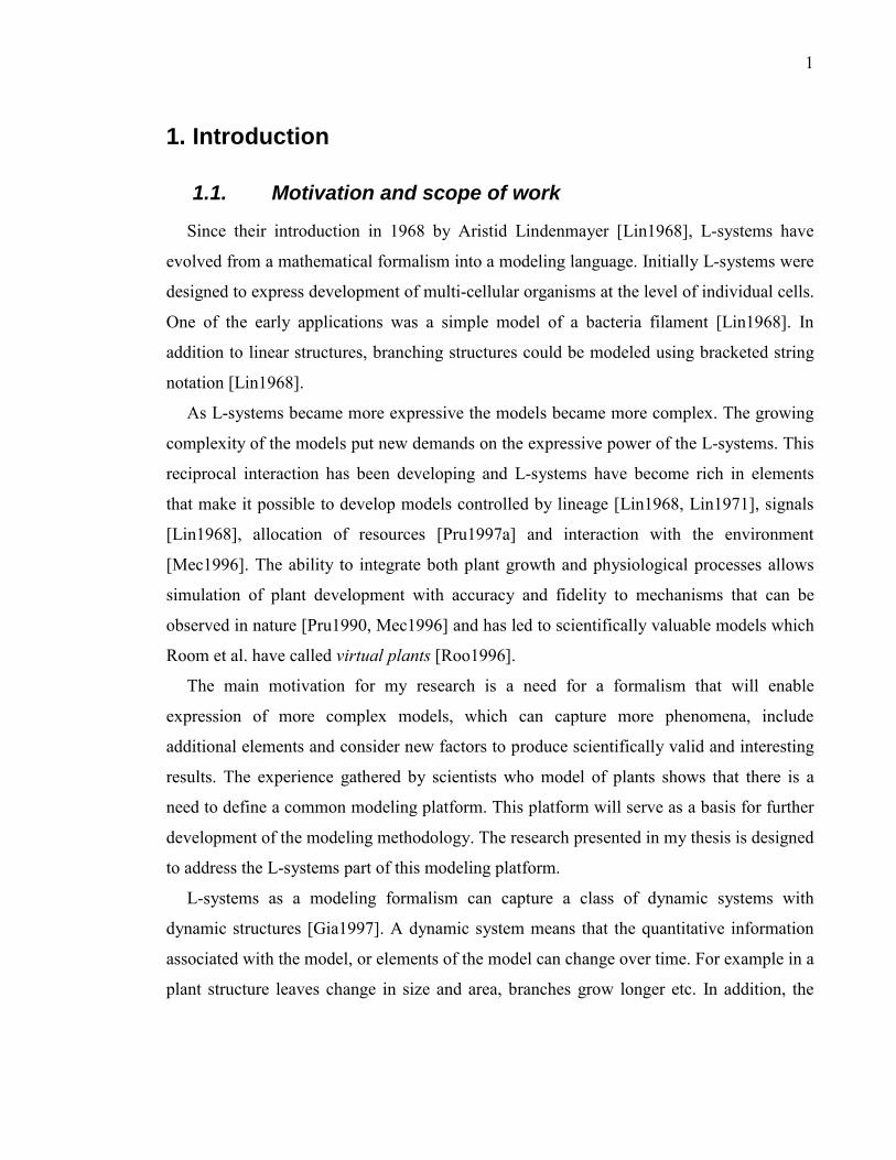
1.1. Motivation and scope of work
Since their introduction in 1968 by Aristid Lindenmayer [Lin1968], L-systems have
evolved from a mathematical formalism into a modeling language. Initially L-systems were
designed to express development of multi-cellular organisms at the level of individual cells.
One of the early applications was a simple model of a bacteria filament [Lin1968]. In
addition to linear structures, branching structures could be modeled using bracketed string
notation [Lin1968].
As L-systems became more expressive the models became more complex. The growing
complexity of the models put new demands on the expressive power of the L-systems. This
reciprocal interaction has been developing and L-systems have become rich in elements
that make it possible to develop models controlled by lineage [Lin1968, Lin1971], signals
[Lin1968], allocation of resources [Pru1997a] and interaction with the environment
[Mec1996]. The ability to integrate both plant growth and physiological processes allows
simulation of plant development with accuracy and fidelity to mechanisms that can be
observed in nature [Pru1990, Mec1996] and has led to scientifically valuable models which
Room et al. have called virtual plants [Roo1996].
The main motivation for my research is a need for a formalism that will enable
expression of more complex models, which can capture more phenomena, include
additional elements and consider new factors to produce scientifically valid and interesting
results. The experience gathered by scientists who model of plants shows that there is a
need to define a common modeling platform. This platform will serve as a basis for further
development of the modeling methodology. The research presented in my thesis is designed
to address the L-systems part of this modeling platform.
L-systems as a modeling formalism can capture a class of dynamic systems with
dynamic structures [Gia1997]. A dynamic system means that the quantitative information
associated with the model, or elements of the model can change over time. For example in a
plant structure leaves change in size and area, branches grow longer etc. In addition, the

2
structure itself can change: apices produce new branches; some branches may die and fall
off.
The focus of my research was to extend the framework of L-systems to address the
growing needs of the ever more complex functional-structural models. To address these
needs I have extended some concepts present in L-systems as a formalism, added concepts
known from other programming languages, and introduced new ones, not found in other
formalisms.
Specifically the notion of parametric L-systems has been extended. Originally
parametric L-systems allowed any number of numerical parameters to be associated with
modules. This has been extended to allow parameters of any type. In particular, a parameter
can be a user-defined structure. To address the need to express complex algorithms and
calculations I have added user-defined functions, a concept common in other programming-
languages.
An extension that is not found in other formalisms is the concept of fast information
transfer. L-systems have supported information transfer using context-sensitive
productions. This is a universal method for transferring any type of information: the
propagation of hormones, nutrients and other signals through the plant. An inherent feature
of this method is that the number of simulation steps required to transfer information from
point A to point B is proportional to the distance between these points measured as the
number of modules between them. This feature becomes a limitation when the speed of
signal propagation is high compared to the growth rate of the structure (for example
propagation of forces and torques in biomechanical models). Fast information transfer
removes this limitation making it possible to transfer signals throughout the whole structure
represented by the L-system string in one simulation step.
The number and weight of extensions postulated in my research made it justified to
design a completely new modeling language. The new language would combine elements
from L-systems and an imperative programming language. For the elements known from
general-purpose programming, such as functions and user-defined data types (structures),
the syntax from C++ was chosen. Rather than extending a modeling language with more
programming elements, my approach is to add L-system elements to C++. Prusinkiewicz

3
and Hanan [Pru1992] presented a similar idea for adding L-systems to C. Their work was
limited to context-free L-systems, without parameters.
By adding elements of L-systems to C++ the whole power of C++ can be used to
describe algorithms and data structures required for a model. Yet the introduction of L-
system constructs changes the structure of the language: the models are declarative in
nature and consist of productions. Therefore the language has been renamed L+C.
In addition to the language, I have designed and implemented the modeling program
lpfg. It executes models specified in the L+C modeling language. The results can be
rendered as a three-dimensional visualization of the model or stored in an external file for
further analysis. I have also created a comprehensive modeling system, L-studio. L-studio
was inspired by the vlab modeling environment originally created by Mercer [Mer1990,
Mer1991] and then extended by Federl [Fed1999]. L-studio combines the functionality of
several programs to create and render complex models, and is compatible with vlab. The
system has proved to be useful for biologists (it is currently being used in approximately
100 locations worldwide).
1.2. Organization of the dissertation
This section outlines the organization of the thesis.
Chapter 2 presents the history of L-systems, including the main concepts, definitions and
applications that are essential to understanding my research. In chapter 3 the new concepts
that I have added to L-systems are presented. The new modeling language created to
include these concepts is presented in chapter 4. Chapter 5 is devoted to some
considerations on how to implement the language and internal representation of the L-
system string. Chapter 6 discusses the interface which is used to communicate between the
modeling program (lpfg) and the translated L+C model. Chapter 7 contains examples that
demonstrate the benefits of using L+C over traditional L-system language.
Chapter 8 describes the L-studio plant modeling environment which I have created in the
scope of my research. There were two principal reasons for creating this environment. First,
there were several ideas related to interactive and visual modeling techniques that could be
tested. In addition there was considerable interest in a system that would work in the MS
Windows environment coming from biologists who use L-system-based simulations as one

4
of their research tools. The description of L-studio emphasizes the interactive and visual
modeling concepts I have introduced or extended.
The conclusions, including a summary of contributions and issues for further research
are presented in chapter 9. Appendix A contains the user�s manual of lpfg modeling
program, based on L+C modeling language.
1.3. Document conventions
Source code listings are printed using fixed-width font.
5
2. Lindenmayer systems Lindenmayer systems (or L-systems) are a mathematical formalism introduced by
Aristid Lindenmayer in 1968 [Lin1968] to model multi-cellular organisms. Ability to
express branching structures (with bracketed strings) made L-systems particularly useful in
modeling plants. The following sections describe the main concepts of L-systems.
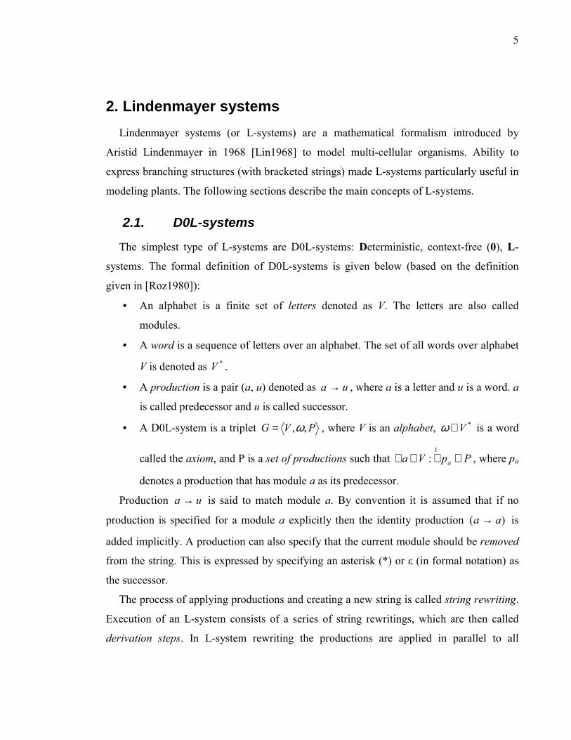
2.1. D0L-systems
The simplest type of L-systems are D0L-systems: Deterministic, context-free (0), L-
systems. The formal definition of D0L-systems is given below (based on the definition
given in [Roz1980]):
• An alphabet is a finite set of letters denoted as V. The letters are also called
modules.
• A word is a sequence of letters over an alphabet. The set of all words over alphabet
V is denoted as *V .
• A production is a pair (a, u) denoted as ua → , where a is a letter and u is a word. a
is called predecessor and u is called successor.
• A D0L-system is a triplet PVG ,,ω= , where V is an alphabet, *V∈ω is a word
called the axiom, and P is a set of productions such that PpVa a ∈∃∈∀1
: , where pa
denotes a production that has module a as its predecessor.
Production ua → is said to match module a. By convention it is assumed that if no
production is specified for a module a explicitly then the identity production )( aa → is
added implicitly. A production can also specify that the current module should be removed
from the string. This is expressed by specifying an asterisk (*) or ε (in formal notation) as
the successor.
The process of applying productions and creating a new string is called string rewriting.
Execution of an L-system consists of a series of string rewritings, which are then called
derivation steps. In L-system rewriting the productions are applied in parallel to all

6
modules in the string. The productions in L-systems are sometimes labelled (pn:) for
presentation or discussion purposes, but the labels do not appear in the actual code.
A classical example of a D0L-system describes the growth of the vegetative segment of
Anabaena catenula [DeK1987, Lin1971]. A vegetative segment consists of cells that can be
in one of two states � young (shorter) or ready to divide (longer). The cells also have two
possible polarities. The polarity specifies which of the daughter cells will be shorter. In the
following L-system (reproduced after [Pru1990]) the letters a and b specify the two states
and the subscripts l and r specify cell polarities.
Listing 1 Development of Anabaena catenula filament.
axiom: ar
p1: ar ! albr
p2: al ! blar
p3: br ! ar
p4: bl ! al
The developmental sequence determined by the L-system in Listing 1 begins with the
axiom ar, and produces a new word with each derivation step:
ar
albr
blarar
alalbralbr
blarblararblarar
2.2. Bracketed L-systems
To represent a branching structure using a string of letters (which by definition is a
linear structure), two reserved modules were introduced as a part of the original definition
of L-systems [Lin1968]. These modules are the left bracket ([) and the right bracket (]) and
they specify the beginning and the end of a branch, respectively.
The following L-system generates a simple branching structure (after [Pru1990], p. 25)
consisting of two types of modules: apices (A) and internodes (I):
7
Listing 2 L-system generating simple branching structure
axiom: A A ! I[A][A]IA I ! II
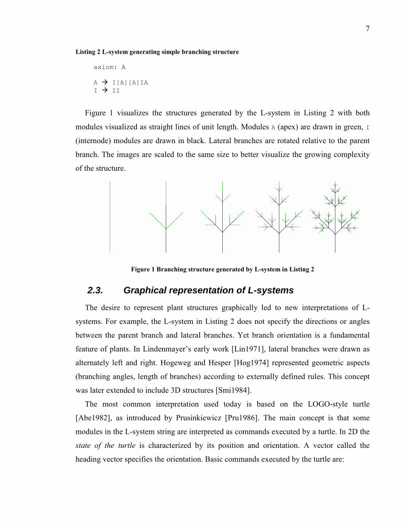
Figure 1 visualizes the structures generated by the L-system in Listing 2 with both
modules visualized as straight lines of unit length. Modules A (apex) are drawn in green, I
(internode) modules are drawn in black. Lateral branches are rotated relative to the parent
branch. The images are scaled to the same size to better visualize the growing complexity
of the structure.
Figure 1 Branching structure generated by L-system in Listing 2
2.3. Graphical representation of L-systems
The desire to represent plant structures graphically led to new interpretations of L-
systems. For example, the L-system in Listing 2 does not specify the directions or angles
between the parent branch and lateral branches. Yet branch orientation is a fundamental
feature of plants. In Lindenmayer�s early work [Lin1971], lateral branches were drawn as
alternately left and right. Hogeweg and Hesper [Hog1974] represented geometric aspects
(branching angles, length of branches) according to externally defined rules. This concept
was later extended to include 3D structures [Smi1984].
The most common interpretation used today is based on the LOGO-style turtle
[Abe1982], as introduced by Prusinkiewicz [Pru1986]. The main concept is that some
modules in the L-system string are interpreted as commands executed by a turtle. In 2D the
state of the turtle is characterized by its position and orientation. A vector called the
heading vector specifies the orientation. Basic commands executed by the turtle are:

8
• F � move forward one unit in the direction specified by the heading vector and draw
a line
• f � move forward one unit in the direction specified by the heading vector without
drawing a line
• + (plus), � (minus) rotate left, right around the position by a predefined angle.
To represent three-dimensional structures the state of the LOGO-style turtle has been
extended. In the 3D systems the orientation of the turtle is defined by three mutually
perpendicular vectors called heading, left and up.
L � left
H � heading
U � up
Figure 2 Turtle orientation defined by vectors H L and U (pointing to the viewer)
The L-system presented below (after [Pru1990]) generates the Koch snowflake using
basic turtle commands. The rotation angle associated with the rotate commands + and � is
specified externally to be 60 degrees.
Listing 3 L-system generating Koch snowflake
Axiom: F--F--F F ! F+F--F+F
Figure 3 Koch snowflake generated by the L-system in Listing 3
Additional commands were also introduced [Pru1986] to make it possible to generate
three-dimensional structures. These commands are
• rotation around the left vector (^ � pitch up, & � pitch down)
• rotation around the heading vector (\ � roll left, / � roll right).

9
When drawing branching structures specified by bracketed L-systems, the modules [ and
] are interpreted as follows:
• ] � the turtle state is pushed on a stack
• [ � the turtle state is popped from the stack.
In addition to the position and orientation the turtle state can also include drawing
parameters, such as drawing colour, line width etc.
2.4. Parametric L-systems
D0L-systems, as presented in the previous sections, can represent qualitative
information in which each type of module represents a different type of components in the
model, such as a cells or organ. Some quantitative information (such as the length of
internodes or the magnitude of angles of rotation) can also be specified by the D0L
formalism using multiple modules to express different lengths of lines or rotation angles.
For example in Listing 3 the two modules + or � are used to represent a rotation of 120
degrees left and right respectively.
However it is impossible to express such a simple figure as an isosceles right triangle
where the line lengths do not have a common denominator. This limitation has been
addressed by parametric L-systems [Pru1990, Han1992].
1
1 2
Figure 4 Isosceles right triangle
The essence of parametric L-systems is that each module consists of a symbol together
with associated numerical parameters. In the productions parameter values are referred to
using formal parameters. Additionally, formal parameters can be used in arithmetic
expressions. The expressions can be used to calculate new values of parameters in the
production�s successors.
The formal definition of parametric D0L-systems is as follows (after [Pru1990]):

10
• V is the alphabet.
• ∑ is the set of formal parameters.
• ( )∑C is the set of all logical expressions with parameters from ∑.
• ( )∑E is the set of all arithmetic expressions with parameters from ∑.
• ( )+ℜ×∈ *Vω is a nonempty parametric word called the axiom.
• P is a finite set of ordered productions of the form pred: condopt ! succ such that
*∑×∈ Vpred , )(∑∈ Ccond and ( )( )**∑×∈ EVsucc . The components of
productions are called predecessor, condition and successor respectively. If the
condition cond is omitted in a production it is assumed to evaluate to true.
In the case of parametric L-systems, the process of matching productions during string
rewriting is more complex than for D0L-systems. For a production to match a module in
the string, the following conditions must be met:
1) The module�s letter must match the letter in the predecessor,
2) The number of actual parameters associated with the module and the number of
formal parameters in the predecessor must be the same,
3) The condition cond must evaluate to true.
For example, production
A(t) : t>5 ! B(t+1)A(t/2)
can be applied to module A(6) and will produce parametric word consisting of two
modules: B(7) A(3).
2.5. Context-sensitive L-systems
In context-free L-systems productions are applied regardless of the context in which the
predecessor module appears. Context-sensitive L-systems make it possible to specify what
modules must be in the neighbourhood of the modules being replaced for the production to
be applied. Context-sensitive L-systems are necessary to express information flow in the
modelled structure. For example the transfer of nutrients or hormones throughout a plant

11
structure can be modelled using context-sensitive L-systems [Lin1968]. Context-sensitive
productions have the form:
lc < pred > rc : cond ! successor
The symbols < and > separate the three components of the predecessor: the left context
(lc), the strict predecessor (pred), and the right context (rc).
The process of matching productions in context-sensitive L-systems is governed by a set
of rules that are discussed in the following section.
2.5.1. How the productions are matched
When rewriting the string it is necessary to determine which production must be applied
to each module in the string. The process of determining the applicable production is called
production matching. For every module in the string, productions are checked for
matching. The productions are checked in the order in which they are specified in the L-
system.
For a production to match, all three components of the predecessor (left context, strict
predecessor and right context) must match. The rules for matching each of these
components are different. This is because the L-system string is a means of representing
branching structures and symmetric operations on the string do not (in general) correspond
to symmetric operations on the branching structure. No good definition of context in
branching structure can be found in the L-systems literature. One of partial definition is the
work by Prusinkiewicz et al. [Pru1988].
This section contains a detailed explanation of rules that control the process of
production matching. Good understanding of these rules is necessary for proper
understanding of the concept of fast information transfer in branching structures (described
in 3.3.2).
When the strict predecessor is compared with the contents of the string in the current
position in order for it to match the modules in the strict predecessor have to match exactly
the modules in the string.

12
When matching the right context and a module in the context is not the same as module
in the string the following rules apply:
• If a module in the string is [ and the module expected is not [ then the branch is
skipped. This rule reflects the fact that modules may be topologically adjacent, even
though in the string representation of the structure the two modules may be
separated by modules representing the lateral branch B (see Figure 5).
• When a branch in the right context ends (with a right bracket) then the rest of the
branch in the string is ignored by skipping to the first unmatched ]. This rule also
reflects the topology of the branching structure, not its string representation. For
example in Figure 6, module C is closer to A than D.
• If multiple lateral branches start at a given branching point, then the predecessor in
Figure 6 would check the first branch (see Figure 7). To skip a branch it is
necessary to specify explicitly which branch at the branching point should be tested
(see Figure 8). This notation is a simple consequence of the rule presented in Figure
6. In the current L-system notation there is no shortcut to specify the second, third
etc. lateral branch in a branching point without explicitly including pairs [ ] in the
production predecessor. There is also no way to specify �any of the lateral
branches�.

13
Skipped branch
Right context
B C
A Current position
String: A [ B ] C
A > C
Skipped branch Strict predecessor
Strict predecessor
Right context
Figure 5 Matching right context, lateral branches are implicitly ignored
Ignored part of the branch
Right context
D
Rest of the branch ignored
BC
A Current position
String: A [ B D ] C
A > [ B ] C
Figure 6 Matching right context, remainder of lateral branch is implicitly ignored
No match
C D
A Current position
String: A [ C ] [ B ] D
A > [ B ] D
B
Figure 7 Problem with multiple lateral branches when matching the right context

14
Branch explicitly ignored
C D
A Current position
String: A [ C ] [ B ] D
A > [ ] [ B ] D
B
Figure 8 Explicit enumeration of lateral branches in the right context
When matching the left context the following rules apply:
• Module [ is always skipped, since the preceding module will be topologically
adjacent (see Figure 9).
• If the module indicates the end of a branch then the entire branch is skipped (Figure
10).
C
B AC < A
Ignored module
String: C [ A ] B
Current position
Left context
Figure 9 Matching left context, beginning of the branch implicitly ignored
C
BA
C < B
Ignored branch
String: C [ A ] B
Current position
Left context
Ignored branch
Figure 10 Matching left context, lateral branches implicitly ignored

15
The rule illustrated in Figure 9 is a pronounced manifestation of asymmetry in the left
context � right context relationship: module C is left context of both A and B. But C�s right
context is B (unless [ ] delimiters are used explicitly). The relation of the left context can be
thought of as the parent module: the module before (below) the branching point. It is then
natural to say that C is parent module for both A and B. The distinction between main
branches and lateral branches can appear to be an implementation dependent artefact, but it
actually can be biologically justified (see for example [Bor1984]).
2.5.2. Ignored and considered modules
The L-system presented below (Listing 4) describes the propagation of an acropetal
signal using a context-sensitive production. This signal can be, for example, a hormone. J
represents an internode where the hormone is present (red line), and I represents an
internode where it is not present (black line).
Listing 4 Acropetal signal propagation implemented using context-sensitive L-system
Axiom: I[+J][-J]J[+J][-J]J[+J][-J]J p1: I < J ! I p2: I+ < J ! I p3: I- < J ! I
Figure 11 Propagation of acropetal signal � output from L-system in Listing 4
The L-system consists of three productions: p1 is responsible for transferring the signal
to the main branches; p2 and p3 are responsible for transferring the signal to the lateral
branches. They are necessary because every J is preceded by a + or a � (the modules that
specify rotation, see section 2.3) and the left context in p1 doesn�t match the sequence of
modules I[+J] or I[-J].

16
Productions p2 and p3 do not add any new information to the model. They have to be
present because of the geometric properties of the model. To be able to abstract from such
details, the notion of ignored modules was introduced. It makes it possible to specify a list
of modules that are ignored when checking for matching context so that Listing 4 can be
rewritten as follows:
Listing 5 Acropetal signal propagation implemented using the ignore statement.
ignore: +- Axiom: I[+J][-J]J[+J][-J]J[+J][-J]J I < J ! I
If the list of ignored modules is long it may be more practical to list only the relevant
modules that appear in the left or right context. This is done using the consider statement.
Consequently Listing 4 can be then rewritten as follows:
Listing 6 Acropetal signal propagation implemented using the consider statement
consider: I Axiom: I[+J][-J]J[+J][-J]J[+J][-J]J I < J ! I
In summary: the presence of ignored and considered modules adds two rules to the test
for matching context.
• When the right context is checked, modules that are not to be considered (those
listed after the ignore keyword or those not listed after the consider keyword) are
skipped (Figure 12).
• Similarly, when checking the left context, ignored modules are skipped (Figure 13).
ignore: X A > C
Ignored module
String: A X C
Current position
Figure 12 Matching right context with ignored modules

17
ignore: X C < A
Ignored module
String: C X A
Current position
Figure 13 Matching left context with ignored modules
2.6. L-systems with programming statements
As the models created using parametric L-systems became more complex, Hanan
[Han1992] extended L-systems to include some programming language constructs (see also
[Pru1992, Pru1996]).
Programming constructs include:
• Assignment of variables (local and global),
• Calls to predefined functions,
• Conditional statements (if � else),
• Loops.
Global variables can be used to store global information about the model e.g. the number
of leaves, flowers. Expressions used in parametric L-systems productions can be
complicated and they are often used in more than one module within one production.
Therefore, local temporary variables were introduced that could store a calculated value
that could be used throughout a production.
A(n) ! F[+A(n+1)][-A(n+1)] (1)
Hanan extended the cpfg language [Han1992] to include the following syntax for
productions:
lc < pred > rc : { α }opt cond { β }opt ! succ

18
where α and β are optional C-like compound statements, and cond is a logical expression.
During the string rewriting if the production predecessor (strict predecessor, left context
and right context) matches the current string position (see section 2.5.1) the statement α (if
present) is executed and cond evaluated. Thus, the production (1) can be rewritten as:
A(n) : { new_n = n+1; } 1 ! F[+A(new_n)][-A(new_n)] (2)
If cond evaluates to true (non-zero) value then β (if present) is executed and the
production applied (the successor added to the new string). But if cond evaluates to zero
then the production is not applied. In this case the next production declared is tested for
matching. This makes it possible to specify more than one production that has the same
predecessor but produces different modules depending on the value of cond. The condition
can depend on the global state of the model (global variables), local conditions (actual
parameters of modules in the predecessor) or both.
Other elements added to the cpfg language by Hanan [Han1992] are predefined
functions that include mathematical functions, pseudo-random number generators etc. They
are used in computations or in file and console I/O operations (results of simulations can be
stored in external files for further analysis using other programs or simply displayed in a
console).
In addition to productions, programming statements can be used in control statements.
Control statements are procedures, which are called during the execution of L-system
program. There are four control statements.
Start: { code } Executed at the beginning of the simulation
StartEach: { code } Executed before each derivation step
EndEach: { code } Executed after each derivation step
End: { code } Executed at the end of the simulation
All control statements are optional.
Listing 7 presents an L-system program that creates a simple branching structure (with
some randomness). The control statements are used to gather statistical data about the

19
model. The data are stored in an external file. Because the L-system source file is
preprocessed using a standard C preprocessor, #define is used to define constants.
Listing 7 L-system with control statements and predefined functions
#define STEPS 50 #define MATURE 1 #define dt 0.2 derivation length: STEPS Start: { fp = fopen("output.dat", "w"); db = 0; step = 0; } StartEach: { ap = 0; step = step+1; } EndEach: { if (ap>0) { fprintf(fp, "%.0f apices created in step %.0f\n", ap, step); } } End: { fprintf(fp, "Total: %.0f dead buds\n", db); fclose(fp); } Axiom: A(0) p1: A(t) : t<MATURE ! A(t+dt) p2: A(t) : ran(1)<0.8 { ap = ap+2; } ! F(0.2)[+A(0)][-A(0)] p3: A(t) : 1 { db = db+1; } ! ,G(0.2); p4: F(t) ! F(1.08*t)

20
Figure 14 Sample image generated by the L-system from Listing 7
There are three global variables declared in the Start statement: fp (file pointer), db
(dead buds counter) and step (step number). Before every derivation step global variable
ap (apex counter) is set to 0 and step is incremented.
Initially the model consists of a young apex A(0). Production p1 increases the age of the
apex until it reaches the mature state (condition t<MATURE). When the apex is mature
production p2 is applied with a 0.8 probability (condition ran(1)<0.8, where ran is a
pseudo-random number generator with uniform distribution). If applied, p2 produces an
internode (module F) and two lateral branches with young apices. It also increments the
global variable ap by two. This variable stores the number of apices produced in every
derivation step. If p2 is not executed then production p3 is applied. In that case the apex is
replaced with a dead bud drawn in an alternate colour1 and the global variable db is
incremented. Production p4 increases the internode length by a constant factor of 1.08. Thus
internodes created earlier will be longer than those created later.
A sample output generated by the L-system from Listing 7 is given below. 2 apices in step 6 4 apices in step 12 6 apices in step 18 8 apices in step 24 12 apices in step 30
1 In cpfg language modules , and ; change the current drawing colour.

21
22 apices in step 36 32 apices in step 42 46 apices in step 48 Total dead buds 21
2.7. Interpretation rules
When creating a plant model it is important to distinguish two elements in the process:
the structure of the plant model and its visualization. For example, during the development
and testing of a model, organs can be visualized simply: stems as straight lines, leaves as
polygons, etc. Once the model generates the correct structure and topology, the visual
aspect can be extended: lines can be replaced with cylinders, and polygons replaced with
3D surfaces (such as Beziér parametric surfaces). If these two aspects can be separated the
model is clearer and easier to maintain. This goal was achieved by introducing
homomorphisms for interpreting the string.
In formal language theory, a homomorphism defines a mapping from an alphabet V to
words in another alphabet Vh [Roz1980]. Formal definition of non-parametric L-systems
with homomorphisms is as follows (after [Pru1997]):
• V and Vh are two alphabets
• PVG ,,ω= is an L-system over alphabet V
• **: hVVh → is a homomorphism
• The ordered quintuplet hPVVH h ,,,, ω= is an L-system with a homomorphism
with the support G and homomorphism h.
Elements of h are called interpretation rules. Interpretation rules are applied only during
the interpretation of the string (for example when visualizing the model2). These rules are
not applied when deriving the string.
The syntax for interpretation rules is the same as productions, except that interpretation
rules are always context-free. During interpretation, modules in the string are replaced with
their image specified by the interpretation rules. By convention, if no interpretation rule is
specified for a module then its image is the module itself. Interpretation rules are applied
2 The string is also interpreted in other cases, for example see 2.9

22
recursively on the resulting words until the word contains only modules that are mapped
into themselves (terminal symbols) or until a predefined recursion depth is reached.
The interpretation rules are more closely related to Chomsky grammars than L-systems.
In Chomsky grammars the productions do not define development but the structure. Also,
productions in L-systems are applied in parallel, whereas productions in Chomsky
grammars are applied sequentially.
The following L-system is an extension of the program presented in Listing 2. It
includes interpretation rules that specify how to draw the organs. An apex is visualized as a
line and a circle3, both drawn using an alternative colour (orange). Internodes are visualized
as straight lines drawn using the default colour (green). In the cpfg language interpretation
rules are preceded by the keyword homomorphism.
3 In cpfg language @o draws a circle

23
Listing 8 L-system from Listing 2 with interpretation rules
#define STEPS 4 derivation length: STEPS axiom: A A ! I[+A][-A]IA I ! II homomorphism A !!!! ;F@o I !!!! F
Figure 15 Image generated by the L-system presented in Listing 8
Figure 16 shows the developmental sequence of a model with interpretation rules. When
the initial string µ0 is visualized, the interpretation rules (h) map this string into the string
v0, which contains the graphical information. After the visualization a derivation step is
performed (P) that applies the productions to the original string µ0 and produce string µ1.
This string is again mapped using the interpretation rules into the string v1 and so on.

24
µ0 P ⇒ µ1
P ⇒ µ2
P ⇒ µ3
P ⇒ �
⇓h ⇓h ⇓h ⇓h v0 v1 v2 v3 ...
Figure 16 Developmental sequence of a model with interpretation rules.
Interpretation rules do not always have to be applied after every derivation step. In some
cases for example the simulation is performed but only the final string is visualized.
2.8. Decomposition rules
Decomposition rules are formally and syntactically related to interpretation rules.
Decomposition rules are context-free. They are also applied recursively. The two
fundamental differences between decomposition and interpretation rules are that the
successor of a decomposition rule is inserted into the string, and decomposition rules are
always applied after each derivation step. Whereas the interpretation rules express the idea
�module looks like this�, decomposition rules express the idea �module consists of the
following�.
µ0 P ⇒ µ0�
D ⇒ µ1
P ⇒ µ 1�
D ⇒ µ2 �
Derivation step Derivation step Figure 17 Developmental sequence of a model with decomposition rules.
Figure 17 shows the developmental sequence of a model with decomposition rules. First
productions (P) are applied and the initial string µ0 is replaced with string µ0�. Then the
decomposition rules (D) are applied and produce string µ1. The string µ0� can be considered
an intermediate state and the application of the decomposition rules can be thought of as a
post-processing phase of the derivation step.
The L-system presented below implements a developmental model of a simple
branching structure.

25
Listing 9 L-system with decomposition and interpretation rules
#define max_t 2 #define dt 0.4 derivation length: 30 Axiom: A(0) p1: A(t) --> A(t+dt) p2: I(t) --> I(t+dt) decomposition d1: A(t) : t>max_t --> I(max_t)[+A(t-max_t)][-A(t-max_t)] homomorphism i1: A(t) --> ;(1)F(t)@o(0.8) i2: I(t) --> ;(2)F(t)
Figure 18 Structure generated by L-system in Listing 9
The model consists of two types of modules: A (apex) and I (internode). Both module
types have one parameter, that represents the age. Initially the model consists of a young

26
apex A(0). The productions p1 and p2 advance time. The actual development is
implemented in the decomposition rule d1. This rule specifies that a mature apex produces
an internode and two lateral apices. This decomposition rule is very similar to the
production p1 from the model presented in Listing 7. The main difference is that the age of
the new apices (as well as the age of the iternode) is calculated as the difference between
the current age of the apex and maximum age. This expresses the idea: if there is an apex of
age t and t>max_t then this apex must have produced an internode and two apices t-
max_t time ago. So the internode and the apices are already that old. This idea can be also
expressed using a production. A production however will not produce correct results if t-
max_t>max_t. For example if max_t=1 then using a production string A(3) would be
replaced with I(2)[+A(2)][-A(2)]. This is wrong because an apex cannot be older than 1,
but because decomposition rules are applied recursively the string A(3) will be properly
decomposed into:
A(3)
I(2)[+A(2)][-A(2)]
I(1)[+A(1)][-A(1)] I(1)[+A(1)][-A(1)]
effectively producing:
I(2)[+I(1)[+A(1)][-A(1)]][-I(1)[+A(1)][-A(1)]]
The fact that decomposition rules are applied recursively makes it possible to create for
example a model of a tree, where every derivation step corresponds to a time step equal to
several years, while branches are produced every year.
Another application of decomposition rules is to generate a sequence of the same (or
similar) modules or groups of modules. For example the decomposition rule in Listing 10
generates n repetitions of the sequence F @o(0.1).

27
Listing 10 Decomposition rule used to generate a sequence of modules
axiom: A(4) decomposition A(n) : n>0 ! F @o(0.1) A(n-1)
After the string is initialized the module A is decomposed into pairs of modules F and @o
followed by an A. The number of repetitions is specified by the value of the actual
parameter of A in the axiom (see Figure 19).
A(4)
F @o(0.1) A(3)
F @o(0.1) A(2)
F @o(0.1) A(1)
F @o(0.1) A(0)
Figure 19 Decomposition rule applied recursively
Effectively the module A(4) is replaced by
F @o(0.1) F @o(0.1) F @o(0.1) F @o(0.1) A(0)
Another decomposition rule can be added to remove the trailing module A(0): A(n) : n==0 ! *
2.9. Environmentally sensitive L-systems and Open L-systems
To model the impact of the environment on plants, and the mutual interaction between
plants and their environment, two extensions to L-systems were made: environmentally
sensitive L-systems and Open L-systems.

28
Environmentally sensitive L-systems [Pru1994] make it possible to pass information
from the environment to the model. Query modules make it possible to access geometric
information about the location and orientation of organs in the model. Query modules are
produced in the axiom or in the production successors. After each derivation step the actual
parameters of all query modules are set and then are used in the next derivation steps.
There are four main query modules: ?P(x, y, z), ?H(x, y, z), ?L(x, y, z) and
?U(x, y, z). They correspond to geometric properties of the LOGO-style turtle: position,
heading vector, left vector and up vector. When a query module is produced its parameters
are set to arbitrary values. After each derivation step the string is interpreted (without
drawing) and if a query module is found its actual parameters are set to the values
corresponding to the current properties of the turtle. This phase is called interpretation for
the environment.
Let us consider the following L-system: Axiom: A p1: A ! F ?P(0, 0, 0) F ?P(0, 0, 0) p2: F > ?P(x,y,z) : 1
{ printf(“Line ends at (%f,%f,%f)\n”, x, y, z); } ! F
Initially the string contains a single module A. During the first derivation step the
contents of the string is replaced with the sequence of four modules:
F ?P(0, 0, 0) F ?P(0, 0, 0).
The query modules ?P have parameters set to 0 as specified in p1. Then the interpretation
for the environment follows. Let�s assume that the turtle�s initial position is (0,0,0) and the
heading vector is (0,1,0). The first module found in the string during the interpretation is F.
This module causes the turtle to move forward in the direction specified by its heading
vector (see 2.3), so its position becomes (0,1,0). The next module found in the string is ?P.
Its three parameters will now be set to the values that represent the turtle�s current position.
So the contents of the string is modified and contains:
F ?P(0, 1, 0) F ?P(0, 0, 0).

29
Then the third module in the string is interpreted (F). It causes the turtle to move forward
again. Now the turtle�s position is (0,2,0). So when the next module is found (?P) its
parameters are changed to contain (0,2,0). After the interpretation for the environment the
string contains:
F ?P(0, 1, 0) F ?P(0, 2, 0).
This ends the first derivation step. During the interpretation for the environment the
contents of the string was changed and the information from the environment acquired. In
the second derivation step the production p2 is applied twice. It doesn�t change the string,
but it prints two messages:
Line ends at (0,1,0)
Line ends at (0,2,0)
To illustrate the use of an environmentally-sensitive L-system a model4 of an extinct
plant Horneophyton ligneri is presented in Listing 11. The main feature captured in the
model is the visible preference of the plant�s branches to grow upwards rather than
horizontally, which results in the characteristic shape of the plant�s crown.
Listing 11 L-system generating a model of Horneopython ligneri
#define SENS 1.0 /* sensitivity to orientation */ derivation length: 7 Axiom: A(10)?H(0,0,0) A(l)> ?H(x,y,z) ! F(l)T
[-(20)/(90)A(l*0.95*y^SENS)?H(0,0,0)] [+(20)/(90)A(l*0.95*y^SENS)?H(0,0,0)]
T ! * homomorphism T ! [-(20)/(90)F(3)][+(20)/(90)F(3)]
4 Unpublished model by P. Prusinkiewicz

30
SENS=0
SENS=1
Figure 20 Image generated by the L-system from Listing 11 for two values of SENS
The presented model proposes a simple mechanism to capture this preference. It
assumes that the length of branches produced by an apex depend on the vertical component
of the apex�s heading vector. It is possible to test the sensitivity of apices to the heading
vector by manipulating parameter SENS that can accept any real-number values. The
length of new branches is multiplied by the expression ySENS, where y is the vertical
component of the apex orientation vector. If, for example, SENS is equal to 0 (no
sensitivity to the orientation), the generated structure presents no directional preference (see
Figure 20 left). When SENS is set to 1 (Figure 20 right) the branches that grow more
horizontally are visibly shorter than the ones growing more vertically.
To obtain the orientation vector of the apex, the query module ?H is used. This module
provides the model with the three components of the heading vector.
Where environmentally sensitive L-systems provide one-way communication from the
environment to the plant model, Open L-systems [Mec1996] make it possible to model bi-
directional interaction between plant and its environment. In this case, the task of modeling
the environment is entrusted to an external program (usually written in a general purpose
programming language such as C). The conceptual model behind open L-systems is
presented in Figure 21.

31
Environment Plant
Reception
Internal processing
Response Reception
Internal processing
Response
Figure 21 Conceptual model of interaction between plant and environment (after [Mec1997])
The internal processing phase in the plant model corresponds to a derivation step (cf.
Figure 21). After each derivation step the string is scanned and communication modules
together with optional additional information (e.g. position and orientation of the module in
3D) are sent to environment. The environment receives this information (reception),
processes the data, and sends its response to the plant model. The plant model receives the
response and is ready for the next derivation step. This feedback loop is continued
throughout the simulation.
The exchange of information between the plant and its environment is done using
communication modules ?E. These modules are similar to the query symbols introduced in
environmentally sensitive L-systems. The main difference is that when communication
modules are generated their actual parameters are the input for the environment. This
information is passed to the environment, which determines its response and sends back
new values of parameters of the communication modules. These new values are then used
in the productions.
To demonstrate how Open L-systems work, I am presenting a real-life example that
demonstrates a phenomenon of canalization [Wad1942]: some organs (petals, primordia) in
capitula are more likely to occur in certain quantities than in others. The model5 presented
in Listing 12 generates a planar, spiral phyllotactic pattern using the algorithm proposed by
5 Unpublished model by P. Prusinkiewicz

32
Vogel in [Vog1979]. The algorithm places consecutive elements of the pattern (the
primordia) using the following formulas:
αϕ ∗= n ncr =
These formulas give the coordinates of pattern elements in the polar coordinates (r,φ). n
is the ordering number and c is a scaling factor. Numbering starts at the centre and proceeds
outward. Battjes and Prusinkiewicz [Bat1995] noticed that when generating phyllotactic
pattern that contains N primordia using the Vogel formula the number of outermost
primordia is usually a number from the Fibonacci series6.
The L-system in Listing 12 generates phyllotactic patterns and demonstrates the effect of
canalization of the number of organs.
Listing 12 Phyllotactic pattern and canalization of number of ray florets
Axiom: A(0) C?E(x): x==0 --> @c C?E(x): x==1 --> ;@c decomposition A(n) : n < NUMBER --> [+(n*137.5)f(0.5*n^0.5)C?E(n)]A(n+1)
6 Fibonacci series is defined as follows: a1=1, a2 =1, an=an-1+an-2 for n>2. The beginning of the series is: 1,
1, 2, 3, 5, 8, 13, 21, 34, 55�

33
Figure 22 Phyllotactic pattern as generated by the L-system from Listing 12
The whole pattern is generated at once in the decomposition rule. Primordia are
represented by modules C followed by a communication module ?E. Each consecutive
primordium has a parameter defining its vigour (n). The vigour is increasing as we move
outward.
To determine which primordia are outermost, an environmental program is used. There
are two pieces of information sent with every communication module ?E: the position of
the primordium (sent implicitly) and its vigour (n). The environment collects this
information and determines which organs are dominant. A dominant organ is one that
collides (occupies the same location in space as another organ) and has vigour that is
greater than the organ with which it collides. The environment sends this information back
by setting the value of the communication module ?E parameter to 0 if the organ is
dominated or to 1 if it is dominant. The dominating primordia are rendered using a different
colour (red).
The simulation presented in Listing 12 was executed for the value of NUMBER in the
range from 2 to 500. The results are shown on the chart on Figure 23. It can be seen that
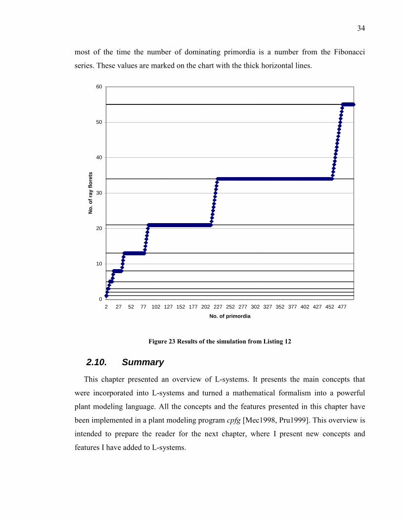
34
most of the time the number of dominating primordia is a number from the Fibonacci
series. These values are marked on the chart with the thick horizontal lines.
0
10
20
30
40
50
60
2 27 52 77 102 127 152 177 202 227 252 277 302 327 352 377 402 427 452 477
No. of primordia
No.
of r
ay fl
oret
s
Figure 23 Results of the simulation from Listing 12
2.10. Summary
This chapter presented an overview of L-systems. It presents the main concepts that
were incorporated into L-systems and turned a mathematical formalism into a powerful
plant modeling language. All the concepts and the features presented in this chapter have
been implemented in a plant modeling program cpfg [Mec1998, Pru1999]. This overview is
intended to prepare the reader for the next chapter, where I present new concepts and
features I have added to L-systems.

35
3. New Concepts and Features in L-systems This chapter presents new concepts and features I have added to L-systems. Sections 3.1
and 3.2 describe why it is useful to extend parametric L-systems with user-defined data
types, and user-definable functions, and how these extensions can be incorporated into the
L-system formalism. In section 3.3 I present further extensions: control of derivation
direction, fast information transfer and a modification of the notion of context: the new
context.
3.1. User-defined data types
The introduction of parametric L-systems [Pru1990, Han1992] made it possible to
include into the models quantitative information that can be expressed by real numbers.
Examples of such information are:
• Geometric properties (length of an internode, diameter of a branch),
• Biologically relevant information (concentration of hormones, amount of nutrients
produced/consumed),
• Biomechanical information (forces, torques, deformations),
For example, let us consider the production:
Listing 13 A sample parametric production
A(x,y) ! B(x+y) C(x-y)
In this production a module of type A with two numerical parameters (x and y) is
replaced by two modules, B and C, which have one parameter each. The values of the
parameters associated with the newly created modules B and C are expressed using standard
arithmetic notation. Specifically, the value of the parameter of module B equals the sum of
parameters x and y of module A, and the parameter of C equals the difference, x-y.
Parametric L-systems made it possible to implement new classes of models. A module
can have any number of parameters. However, n practice, if the number of parameters
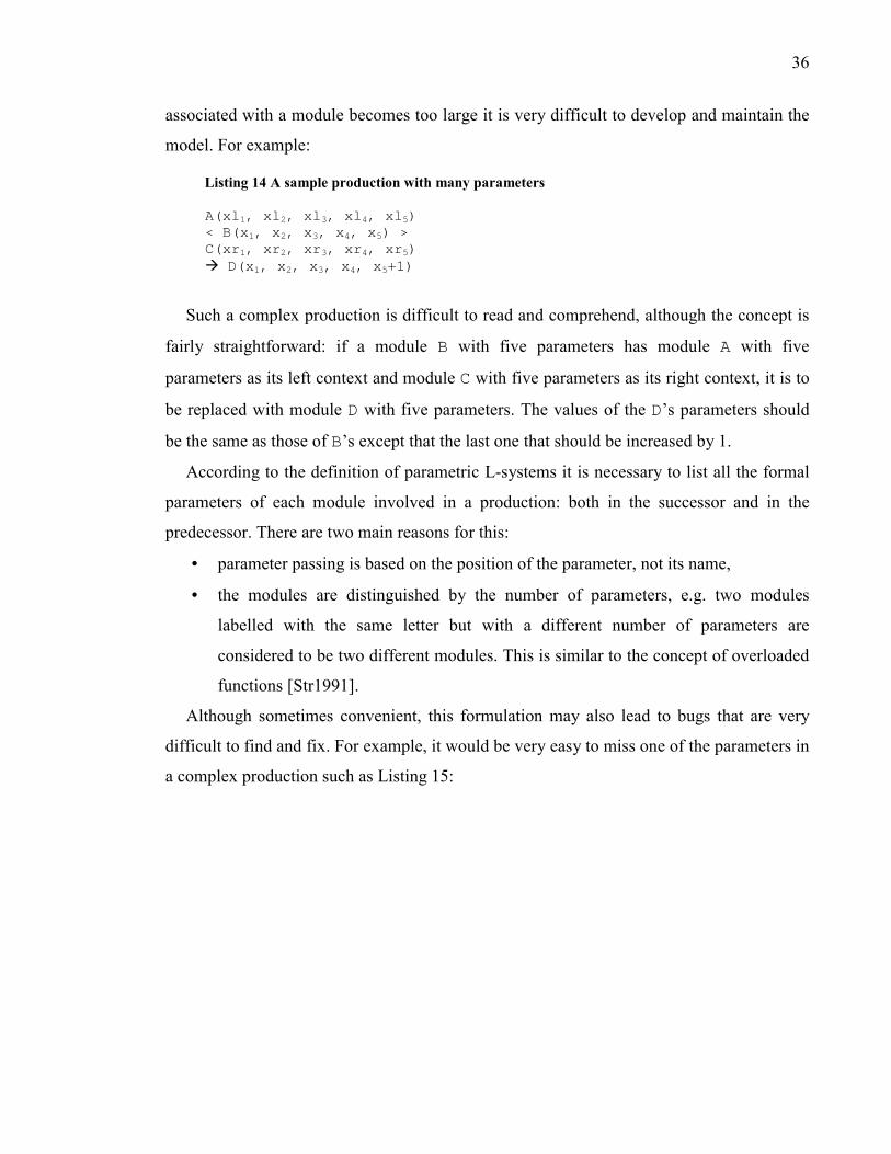
36
associated with a module becomes too large it is very difficult to develop and maintain the
model. For example:
Listing 14 A sample production with many parameters
A(xl1, xl2, xl3, xl4, xl5) < B(x1, x2, x3, x4, x5) > C(xr1, xr2, xr3, xr4, xr5) ! D(x1, x2, x3, x4, x5+1)
Such a complex production is difficult to read and comprehend, although the concept is
fairly straightforward: if a module B with five parameters has module A with five
parameters as its left context and module C with five parameters as its right context, it is to
be replaced with module D with five parameters. The values of the D�s parameters should
be the same as those of B�s except that the last one that should be increased by 1.
According to the definition of parametric L-systems it is necessary to list all the formal
parameters of each module involved in a production: both in the successor and in the
predecessor. There are two main reasons for this:
• parameter passing is based on the position of the parameter, not its name,
• the modules are distinguished by the number of parameters, e.g. two modules
labelled with the same letter but with a different number of parameters are
considered to be two different modules. This is similar to the concept of overloaded
functions [Str1991].
Although sometimes convenient, this formulation may also lead to bugs that are very
difficult to find and fix. For example, it would be very easy to miss one of the parameters in
a complex production such as Listing 15:
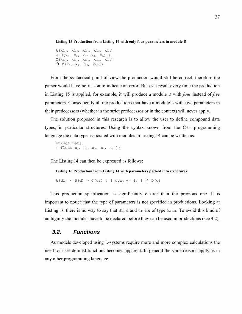
37
Listing 15 Production from Listing 14 with only four parameters in module D
A(xl1, xl2, xl3, xl4, xl5) < B(x1, x2, x3, x4, x5) > C(xr1, xr2, xr3, xr4, xr5) ! D(x1, x2, x3, x5+1)
From the syntactical point of view the production would still be correct, therefore the
parser would have no reason to indicate an error. But as a result every time the production
in Listing 15 is applied, for example, it will produce a module D with four instead of five
parameters. Consequently all the productions that have a module D with five parameters in
their predecessors (whether in the strict predecessor or in the context) will never apply.
The solution proposed in this research is to allow the user to define compound data
types, in particular structures. Using the syntax known from the C++ programming
language the data type associated with modules in Listing 14 can be written as: struct Data { float x1, x2, x3, x4, x5 };
The Listing 14 can then be expressed as follows:
Listing 16 Production from Listing 14 with parameters packed into structures
A(dl) < B(d) > C(dr) : { d.x5 += 1; } ! D(d)
This production specification is significantly clearer than the previous one. It is
important to notice that the type of parameters is not specified in productions. Looking at
Listing 16 there is no way to say that dl, d and dr are of type Data. To avoid this kind of
ambiguity the modules have to be declared before they can be used in productions (see 4.2).
3.2. Functions
As models developed using L-systems require more and more complex calculations the
need for user-defined functions becomes apparent. In general the same reasons apply as in
any other programming language.

38
• Functions encapsulate calculations. When a function is defined the calculations are
separated from the rest of the program. At the same time the complexity of the
calculations does not obstruct the main code.
• Functions are reusable: some formulas (or algorithms) are used in more than one
place in a model. A simple call to the function can be used rather than repeating the
details of the algorithm each time.
Well-designed functions have meaningful names and good parameters that can give
information about what the function actually does and what is the meaning of the
parameters. When an algorithm is included in the main code it is necessary to look
at the implementation to find out what it does. By using a function, a person reading
the model can understand what the algorithm does, without having to know how it
does it.
• Functions can be much more expressive than arithmetic formulas. Some languages
that do not support functions include simple macros (in the C preprocessor sense)
for representing calculations7. For example:
#define VectorLength(x, y, z) sqrt(x*x+y*y+z*z)
However no loops or conditional statements can be used in macros.
• Functions can be combined into libraries: Some functions are used in different
models. For example functions that calculate the dot product of vectors and the
length of vectors are general in nature and are used in different models. Instead of
rewriting them one can group such functions into a library that can be linked to
different models.
The calculations of L-systems do not require any special syntax. It is therefore
reasonable to assume that the syntax from any general-purpose language is acceptable.
3.3. Fast information transfer
The importance of information transfer in biological models cannot be overstated. For
example, information transfer (or signal propagation) in L-system models is used to model
7 C preprocessor is used for example by rayshade. A mechanism similar to C preprocessor is also used in
POV-ray.
39
the transport of substances in the plant, such as hormones, nutrients. It is also used for
collecting information about the structure, such as number of apices supported by a given
branch, and biomechanical information such as the: sum of forces, momentums, and
torques acting on a branch. Information can be transferred using context-sensitive
productions but this mechanism may not be fast enough in some applications. In the
following sections I present the traditional approach to the problem and then introduce a
new method, which I call fast information transfer.
3.3.1. Information transfer in linear structures
This section discusses the problem of information transfer in linear structures. First the
traditional approach using context-sensitive productions is presented in 3.3.1.1. Then the
new method using fast information transfer is shown in 3.3.1.2.
3.3.1.1. Traditional approach
Context-sensitive L-systems as introduced by Lindenmayer [Lin1968] have been a
natural choice for expressing information transfer. For example the L-system in Listing 17
moves a signal from left to right through the series of A modules, counting the number of
A�s.
Listing 17 Information transfer in linear structure using context-sensitive productions
axiom: S(0) AAAAAAAA S(n) < A ! A S(n+1) S(n) > A ! ε S(n) ! R(n)
S has one parameter, which represents the number of A�s counted so far. In the axiom
this value is set to 0. After the first derivation step module S will move past the leftmost A
and the value of its parameter will be 1:
AS(1) AAAAAAA
After the next derivation step S will move past the second A and the value of its
parameter will increment:

40
AAS(2) AAAAAA
Eventually after eight steps module S will reach the end and will be replaced with
module R representing the final result.
AAAAAAAA R(8)
It takes N derivation steps to transfer the signal (the counter module S) from one end of
the string to the other, where N is the number of A�s. Because the time required to perform a
single derivation step is also proportional to N, this method of transferring information is
O(N2).
3.3.1.2. Fast information transfer
According to the original formulation of L-systems the modules in the string are
replaced with their successors simultaneously. Nevertheless, in practice the process of
derivation is usually performed sequentially. The original string is scanned, module by
module, and as the productions are applied the new string is built. If the user knows that the
process of derivation is performed in a given direction (for example from left to right) it is
possible to rewrite Listing 17 as follows:
Listing 18 Fast information transfer in a linear structure, using a global variable
n = 0; axiom: AAAAAAAA p1: A > A : { n++; } ! A p2: A : { n++; } ! A R(n)
In a single derivation step, the first production replaces each module A that has another
module A to the right with itself, while the second production handles the end case. Both
productions increment n as each A is replaced. The table below shows the execution of a
single derivation step. The first column shows the contents of the original string and the
current module is shown in boldface.

41
Original string Production applied n Resulting string
AAAAAAAA p1 1 A
AAAAAAAA p1 2 AA
AAAAAAAA p1 3 AAA
AAAAAAAA p1 4 AAAA
AAAAAAAA p1 5 AAAAA
AAAAAAAA p1 6 AAAAAA
AAAAAAAA p1 7 AAAAAAA
AAAAAAAA p2 8 AAAAAAAA R(8)
In this way the signal propagates through the string in a single derivation step and the
string is only scanned once. Since the time required to perform a derivation step is
proportional to the number of modules in the string, this method is O(N).
If a signal needs to be propagated from right to left, the analogous method can be
applied as long as the derivation can be performed from right to left. So here I am
introducing the term derivation direction. I assume that the process of string rewriting is
done sequentially. The derivation direction specifies whether during rewriting the string is
scanned from left to right (forward) or from right to left (backward).
The information propagation presented in this section is an example of using the fast
information transfer in a linear structure. The only overhead in this method compared to the
traditional method is the need for a global variable (n). To use the fast information transfer
method, the derivation direction must be controlled by the user.
3.3.2. Information transfer in branching structures
Examples from the previous sections can be extended to branching structures where it is
often necessary to count the branching order to determine features such as the age of a
branch or its distance from the base. Berntson [Ber1997] presented a number of topological
ordering schemes, which can be divided into two broad categories: (developmental)
centrifugal and (functional) centripetal.
When labelling segments according to a developmental scheme, the process starts at the
base of the system and orders are assigned in increasing magnitude away from the base.
The name developmental reflects the direction of growth of the branching (or root) system.

42
When a functional scheme is used, the process starts at the tips of the branches (or root
tips) and orders of increasing magnitude are assigned toward the base. This scheme reflects
the distance (especially topological distance) to the base and is usually correlated with age
of the organ.
Two different labelling schemes will be applied on simple branching structures. One of
the schemes requires a signal to be propagated from tips of branches to the root and the
other requires the signal to go from the base of the structure to the tips. Both labeling
schemes will be first implemented using context-sensitive L-systems and then using fast
information transfer.
Here is a sample branching structure:
ab
A
B
C
D
E
ce
d
Figure 24 A sample branching structure
The structure in the Figure 24 corresponds to the following string: I[I[IAe]IAd]I[IAc]I[IAb]IAa
Modules I represent internodes (lines). Modules A represent apices (circles). The indices
associated with modules of type A have been added only to help identify the modules on the
diagram and those in the string. Branching points are visualized as diamonds and are
labelled with capital letters. Internodes that are lateral to their parent branch are thinner
than main branches. For example the internode between the branching points D and B is a
main branch, whereas the internode from B to the apex c is lateral. On the other hand
internode D C is lateral to its parent (E D), but the internode from C to apex d is the main

43
branch for D C. The distinction between the main and lateral branches will become relevant
when implementing developmental labelling scheme in the section 3.3.2.2.
3.3.2.1. Traditional approach
Developmental labelling scheme
In the case of developmental labelling schemes the signal needs to be propagated from
the root to the tips. The root as the oldest part of the plant has number 1. All child branches
(main or lateral) have numbers based on the label of their parent incremented by one.
The L-system that performs the labelling contains two productions:
Axiom: I[I[IAe]IAd]I[IAc]I[IAb]IAa
p1: I(parent)< I(n) ! I(parent+1)
p2: I(n) ! I(1)
And this is how it proceeds:
1
1
1
1
1 1
1
1
1
(a)
a
b
A
c
d
e
B
C
E
D
2
2
2
2
2 2
2
2
1
(b)
a
b
A
ce
dB
C
D
E
3
3
3
3
3 3
2
2
1
(c)
a
b
A
ce
dB
C
D
E
3
3
3
3
4 4
2
1
(d)
a
b
A
c e
dB
C
2 D
E
Figure 25 Information transfer in a branching structure from the root to the tips
Red lines represent the internodes, which contain updated information. The number of
steps required to propagate the information is equal to the length of the longest branch.
Functional labelling scheme
This labelling scheme can be used to calculate the number of apices supported directly
or indirectly by every internode. Every module representing an internode I will have a
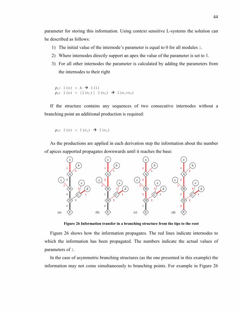
44
parameter for storing this information. Using context sensitive L-systems the solution can
be described as follows:
1) The initial value of the internode�s parameter is equal to 0 for all modules I.
2) Where internodes directly support an apex the value of the parameter is set to 1.
3) For all other internodes the parameter is calculated by adding the parameters from
the internodes to their right
p1: I(n) > A ! I(1) p2: I(n) > [I(n1)] I(n2) ! I(n1+n2)
If the structure contains any sequences of two consecutive internodes without a
branching point an additional production is required:
p3: I(n) > I(n1) ! I(n1)
As the productions are applied in each derivation step the information about the number
of apices supported propagates downwards until it reaches the base:
1
0
1
1 1
0
0
0
(a)
a
b
A
c e
d
1 C
B
D
E
1
1
2
1
1 1
2
1
0
(b)
a
b
A
e
dB
C
D
E
c
1
1
2
1
1 1
2
3
3
(c)
a
b
A
ce
dB
C
D
E
1
1
2
1
1 1
2
3
5
(d)
a
b
A
c e
dB
C
D
E
Figure 26 Information transfer in a branching structure from the tips to the root
Figure 26 shows how the information propagates. The red lines indicate internodes to
which the information has been propagated. The numbers indicate the actual values of
parameters of I.
In the case of asymmetric branching structures (as the one presented in this example) the
information may not come simultaneously to branching points. For example in Figure 26
45
(a) the information has reached point B only from c but not from A. In (b) the information
has reached the point B but D is still waiting, etc.
It is imperative to be able to determine whether information has reached a certain point
and yet this is a non-trivial task. For example, checking if the value is non-zero can be
misleading (e.g. the parameter of internode DB in figure (b) or the parameter of internode ED
in figure (c) are non-zero but do not contain the correct values). In practice it is necessary to
use an additional parameter (flag) to indicate if the information has reached the given point.
The number of steps required to propagate a signal in a branching structure is equal to
the length of the longest branch (main or lateral).
3.3.2.2. Fast information transfer with a stack
In the case of a branching structure, a single variable is usually not enough to apply fast
information transfer. Instead a stack is required. It is assumed that there is a data structure
theStack, which implements a stack of integers. theStack implements three methods:
void Push(int) and int Pop() (removes the top element from the stack) and int Top()
(returns the value of the top element without removing it).
Developmental labelling scheme
To propagate a developmental signal in a branching structure it is necessary to be able to
distinguish between main and lateral branches. The derivation must be performed forward.
In the following L-system the second parameter of I indicates main and lateral internodes.
It is true (1) for the main internodes and false (0) for the lateral ones:
Listing 19 Fast information transfer applied to a developmental signal in a branching structure
p1: I(nl, sl) < I(n,s) : { if (s==true) newn = theStack.Pop()+1; else newn = theStack.Top()+1; theStack.Push(newn); } ! I(newn, s) p2: I(n,s) < A() : { theStack.Pop(); } ! A

46
p3: I(n,s) : { theStack.Push(1); } ! I(1,s)
When a new value of I�s first parameter is set (p1 and p3) this value is pushed on the
stack. When the value of the previous label is needed (p1) it is accessible as the top element
on the stack.
This value is only read when the current internode is a lateral branch and is read and
removed from the stack when the current internode is a main branch. This is because every
lateral branch precedes a main branch in the string. To analyze how this L-system works a
simpler branching structure was chosen (see Figure 27).
I3
I2
I1
I1[I2A]I3A
Figure 27 Sample branching structure
The table below shows the progress of a single derivation step performed on the string
representing the branching structure (Figure 27). In the first column the current module is
indicated in boldface. The third column shows the contents of the stack after the production
specified in the second column has been applied. Original string Production
applied Stack Resulting string
I1(0,1)[I2(0,0)A]I3(0,1)A p3 1 I1(1,1)
I1(0,1)[I2(0,0)A]I3(0,1)A p1 2 1
I1(1,1)[I2(2,0)
I1(0,1)[I2(0,0)A]I3(0,1)A p2 1 I1(1,1)[I2(2,0)A I1(0,1)[I2(0,0)A]I3(0,1)A p1 2 I1(1,1)[I2(2,0)A]I3(2,1) I1(0,1)[I2(0,0)A]I3(0,1)A p2 Empty I1(1,1)[I2(2,0)A]I3(2,1)A
Every internode (except the first one) uses the information from the stack to calculate its
own order. Also productions push the order value on the stack to be used by the next
internode. Terminal internode values are not used; therefore they must be removed from the
stack (p2). Also every production for a main internode removes the top element from the
stack, as it is no longer used.

47
Functional labelling scheme
This L-system implements the functional scheme presented in 3.3.1.2 using fast
information transfer.
Listing 20 Fast information transfer in a branching structure using a global stack
p1: I(n) > A : { theStack.Push(1); } ! I(1) p2: I(n) > [I(nl)] I(ns) : { n = theStack.Pop() + theStack.Pop(); theStack.Push(n); } ! I(n)
This L-system assumes that the derivation is performed backwards � from right to left.
This is how the process proceeds on the branching structure presented in Figure 27. Original string Production
applied Stack Resulting string
I1(0)[I2(0)A]I3(0)A p1 1 I3(1)A
I1(0)[I2(0)A]I3(0)A p1 1 1
I2(1)A]I3(1)A
I1(0)[I2(0)A]I3(0)A p2 2 I1(2)[I2(1)A]I3(1)A
The algorithm is based on the fact that the branch tips are visited before the branching
points. When a branching point is visited, the stack contains the values pushed by the
productions applied for the internodes at the tips. Every internode pushes the value of its
parameter on the stack. Internodes at the tips (those that have an apex in the right context)
set the value of the parameter to 1. Internodes at the branching points calculate the value of
the parameter based on two topmost values on the stack. This method resembles the way
arithmetic expressions are calculated using the reverse Polish notation.
3.3.2.3. Fast information transfer using the new context
The method presented in the previous sections requires a global data structure � the
stack. The stack contains data that are a subset of the information that is generated in
successors. But in fact these data are redundant as they are already present in the new string
being created.
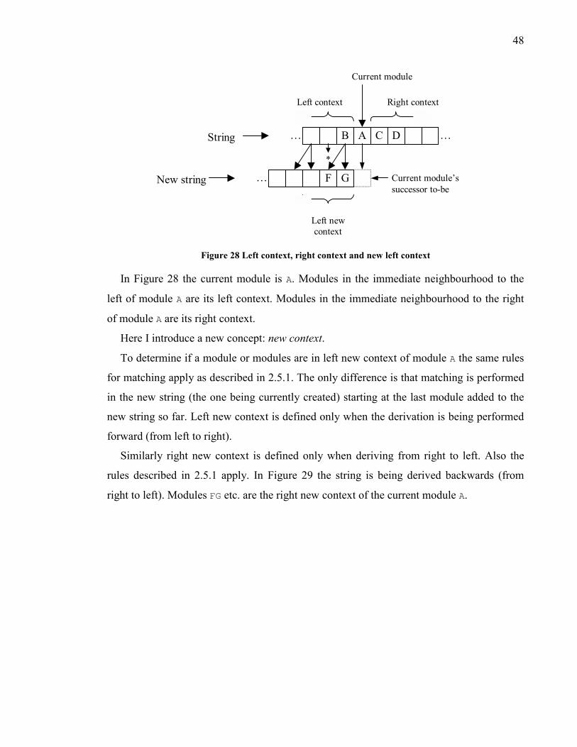
48
Left context
*
A CB� � D
GF
Current module
� Current module�s successor to-be
Right context
Left new context
String
New string
Figure 28 Left context, right context and new left context
In Figure 28 the current module is A. Modules in the immediate neighbourhood to the
left of module A are its left context. Modules in the immediate neighbourhood to the right
of module A are its right context.
Here I introduce a new concept: new context.
To determine if a module or modules are in left new context of module A the same rules
for matching apply as described in 2.5.1. The only difference is that matching is performed
in the new string (the one being currently created) starting at the last module added to the
new string so far. Left new context is defined only when the derivation is being performed
forward (from left to right).
Similarly right new context is defined only when deriving from right to left. Also the
rules described in 2.5.1 apply. In Figure 29 the string is being derived backwards (from
right to left). Modules FG etc. are the right new context of the current module A.
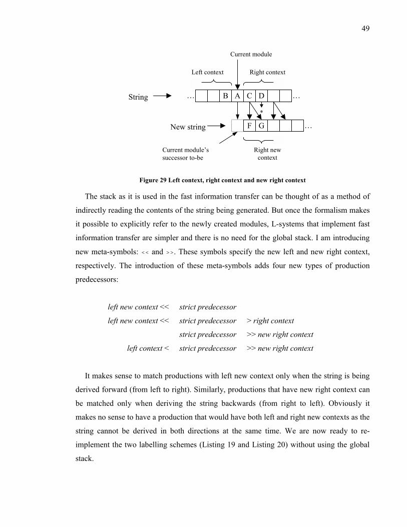
49
Left context
*
A CB� � D
GF
Current module
�
Current module�s successor to-be
Right context
Right new context
String
New string
Figure 29 Left context, right context and new right context
The stack as it is used in the fast information transfer can be thought of as a method of
indirectly reading the contents of the string being generated. But once the formalism makes
it possible to explicitly refer to the newly created modules, L-systems that implement fast
information transfer are simpler and there is no need for the global stack. I am introducing
new meta-symbols: << and >>. These symbols specify the new left and new right context,
respectively. The introduction of these meta-symbols adds four new types of production
predecessors:
left new context << strict predecessor
left new context << strict predecessor > right context
strict predecessor >> new right context
left context < strict predecessor >> new right context
It makes sense to match productions with left new context only when the string is being
derived forward (from left to right). Similarly, productions that have new right context can
be matched only when deriving the string backwards (from right to left). Obviously it
makes no sense to have a production that would have both left and right new contexts as the
string cannot be derived in both directions at the same time. We are now ready to re-
implement the two labelling schemes (Listing 19 and Listing 20) without using the global
stack.

50
Developmental labelling scheme
An L-system using the fast information transfer with new context that implements the
developmental labelling scheme contains two productions is presented below:
Listing 21 Developmental labelling scheme implemented using fast information transfer with new
context
p1: I(nl) << I(n) ! I(nl+1) p2: I(n) ! I(n+1)
The process of rewriting is shown in the table below: Original string Production applied Resulting string
I(0)[I(0)A]I(0)A p2 I(1)
I(0)[I(0)A]I(0)A p1 I(1)[I(2)
I(0)[I(0)A]I(0)A identity I(1)[I(2)A
I(0)[I(0)A]I(0)A p1 I(1)[I(2)A]I(2)
I(0)[I(0)A]I(0)A identity I(1)[I(2)A]I(2)A
The L-system using the new context has the following advantages:
• There is no need for the stack
• It needs just one production (production p2 merely initializes the first internode�s
parameter to 1)
• There is no need for an extra parameter to distinguish between main and lateral
branches
Functional labelling scheme
The L-system in Listing 22 implements the functional labelling scheme using the new
context. The derivation is performed backwards.
Listing 22 Functional labelling scheme implemented using the new context
p1: I(n) > A ! I(1) p2: I(n) >> [ I(nl) ] I(ns) ! I(nl+ns)
The table below shows the process of rewriting

51
Original string Production applied Resulting string I(0)[I(0)A]I(0)A identity A
I(0)[I(0)A]I(0)A p1 I(1)A
I(0)[I(0)A]I(0)A identity A]I(1)A
I(0)[I(0)A]I(0)A p1 I(1)A]I(1)A
I(0)[I(0)A]I(0)A p2 I(2)[I(1)A]I(1)A
3.4. Summary
This chapter presents the extensions I have added to the formalism of L-systems. The
extensions include two features known from general purpose languages: user-defined data
types and functions. These features extend the capabilities of L-systems in expressing
models that require many parameters and complex calculations.
A new concept, not found in other formalisms is the concept of fast information transfer.
Fast information transfer together derivation direction and new context make it possible to
transfer signals through the structure represented by the L-system string in a single
derivation step.
All these extensions and concepts have been incorporated in the modeling language
L+C, which is described in the following chapter.

52
4. The Modeling language L+C The number and significance of the new features and concepts that I have added to the
formalism of L-systems made it desirable to design a new language instead of extending the
existing implementation of the plant modeling language cpfg. This is why I have designed
modeling language L+C8. This language is a declarative language based on the formalism
of L-systems.
L+C combines constructs, which can be divided into two categories:
a) constructs specific to L+C
b) constructs known from other programming languages, in particular the C++ general
purpose programming language.
The syntax of the constructs that are not characteristic to L-systems has been borrowed
from C++. This includes rules for scoping. Contents specific to L-systems have syntax,
which is partially inherited from the traditional notation of L-systems, but also some effort
has been made to use syntax that would not look too alien to C++. The decision of
designing L+C based on the syntax of C++ gives the following benefits:
• the learning curve is gentle for people who already know C++,
• the expressive power of C++ together with existing methodologies and libraries can
be used directly in an L+C program,
• no documentation is needed for the C++ part of the language.
A program in L+C consists of a series of declarations:
• Structures, classes
• Global variables
• Functions
• Derivation length
• Modules
8 First draft of the language specifications, has been prepared together with P. Prusinkiewicz, R. Sievänen
and J. Perttunen and described in an unpublished manuscript.

53
• Axiom
• Productions
• Decomposition rules
• Interpretation rules
• Control statements
This chapter discusses the syntax of L+C. As the syntax of C++ constructs is the same as
in C++, only the syntax of constructs specific to L+C will be presented. Listings in this
chapter show sample uses of the constructs being presented.
4.1. Derivation length
Derivation length specifies the number of derivation steps.
derivation length: expression;
4.2. Module declarations
L+C requires that all modules used in a model must be declared. Modules are identified
by their names (identifiers). Two modules are predefined in L+C: SB and EB. SB is the start
of a branch and EB is the end of a branch. These modules correspond to the modules [ and ]
in the traditional notation.
Module declaration has the following syntax:
module identifier(parameter-listopt);
The identifier must be a valid C++ identifier. The parameter list is an optional list of
type identifiers separated by commas. The following listing presents some sample module
declarations:
Listing 23 Examples of module declarations
struct data { int n; float arr[3];

54
}; // module without parameters module A(); // module with two parameters module C(int, float); // module with a parameter of user-defined structure type data module Internode(data);
Types that are used as module parameter types must be defined beforehand.
4.3. Axiom
Axiom defines the initial contents of the L-system string. There must be exactly one
axiom declared in every L-system. The syntax of the axiom is as follows:
axiom: parametric-wordopt;
A parametric word is a sequence of one or more parametric modules:
identifier(expression1, expression2, ...)
Where identifier must be name of a previously declared module. The number of
expressions in the parenthesis must be the same as the number of parameters in the
module�s declarations. Also, the types of expressions must correspond to the types of
parameters in the module�s declaration. If the parameter is declared to have no parameters
(as module A in Listing 23), then the module�s identifier is followed by (). Optionally the
parentheses might be skipped altogether.
If modules A, C and Internode are declared as in Listing 23 a sample axiom may look
like this:
axiom: A C(i, 2.3) Internode(d);
Here, i must be an integer and d must be a variable of type data. The same syntax of
parametric word is also used in the produce statement.

55
4.4. Productions
Productions define the way the structure represented by the L-system string develops
over time by specifying the fate of every module. Declaration of a production starts with
the predecessor. The predecessor consists of three components: the strict predecessor, the
left context and the right context (see 2.5). The left context and the right context are
optional. Also, one of the new contexts (left or right) can be specified in a production
predecessor (see section 3.3.2.3). The strict predecessor specifies which module(s) in the
string will be replaced.
Left and right context specify which modules must be present in the neighbourhood of
the strict predecessor. The general syntax for productions is:
leftcontextopt < newleftcontextopt << strictpred >> newrightcontextopt > rightcontextopt:
{
production body }
All components of a production predecessor are sequences of one or more modules with
formal parameters, such as those shown in the following example:
Listing 24 Example of production predecessor in L+C
A() < C(i, r) > Internode(d)
This predecessor specifies that the production should be applied to module C if there is a
module A to the left of C and a module Internode to the right. The types of parameters are
determined by the declarations of modules, which have to appear before the modules are
used in a production. If the modules A, C and Internode are declared as in Listing 23 then
i will be an integer, r will be a float and d will be a structure of type data. All formal
parameters of every module must be listed, even if they are not used in the production
body. The identifiers of formal parameters must be unique within a production. Their scope
is the same as the scope of formal parameters in C++ functions.

56
Formal parameters are similar to formal parameters of functions. When a production is
applied they are given values. These values can be used inside the production body.
In the case of a production, the formal parameters get the values from the actual
parameters of modules in the string. For example, if the string contains the following
sequence:
A C(5, 2.5) I({ 2, { 0, 0.4, 0.6 }})
the production from Listing 24 can be applied. The production formal parameters will be
assigned the following values:
i = 5, r = 2.5, d = { 2, { 0, 0.4, 0.6 }}
A program in L+C can define more than one production for the same module. In other
words more than one production can refer to the same module in the strict predecessor.
Listing 25 Sample production predecessors in L+C
A() < C(i, r) > Internode(d) : { … } C(i, r) > Internode(d) : { … } C(i, r) : { ... }
When more than one production is declared for a given module, the order in which these
productions are specified is important. When the string is being rewritten, then for every
module in the string a production must be applied. If there is more than one production for
a given module then the productions will be tested for matching in the order in which they
are declared. In Listing 25 there are three productions for module C. The first one specifies
both the left and right context, the second specifies only the right context and the third one
is context-free.

57
According to the original definition [Lin1968] productions are applied in parallel. In
L+C the derivation is performed sequentially9. It can be performed in one of two directions:
forward (from left to right) or backward (from right to left) (see 3.3).
Because the derivation is performed in a specified direction and this direction can be
controlled, L+C allows the use of the new context (see 3.3.2.3). The syntax used for
specifying the new context is the same as that used with ordinary context. Checking for
new and ordinary context can be mixed in one production, as in the following examples:
A() < C(i, r) >> Internode(d) : … A() < A() << C(i, r) > Internode(d) : … A() << C(i, r) : ... A() < C(i, r) >> Internode(fd) > Internode(d) : ...
etc.
As explained in section 3.3.2.3 checking for right new context makes sense and is
possible only when the string is being derived from right to left. If the derivation is being
performed in the opposite direction, these productions are ignored. Similarly, checking for
the left new context is possible only when the string is being derived from left to right and
this is the only time when these productions are tested for matching. The derivation
direction is controlled by the user form within L-system (see A.6.13). Discussion of the use
of new context is presented in section 3.3.2.3.
A production successor is specified using the produce statement. The syntax of the
produce statement is presented in the following section.
4.5. The produce statement
A production consists of the predecessor and the body. The production body is a
compound statement that can contain any code allowed inside a C++ function. In addition,
9 As a matter of fact, the introduction of the cut module [Han1992] silently implies that the process of
derivation is performed sequentially from left to right.
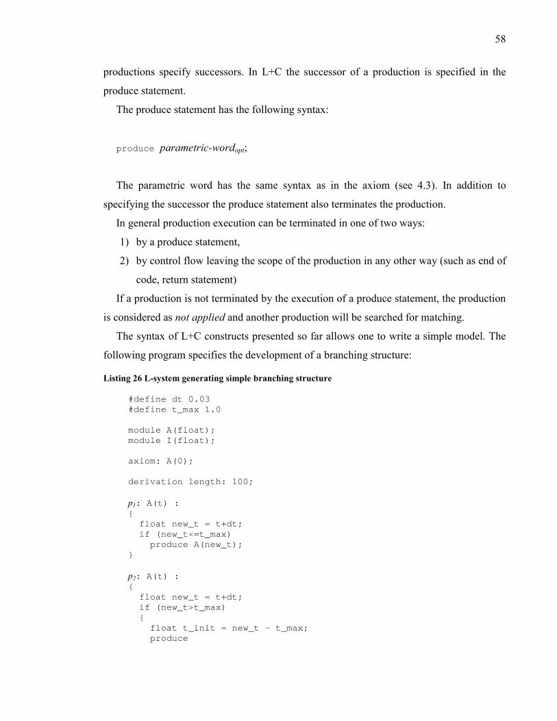
58
productions specify successors. In L+C the successor of a production is specified in the
produce statement.
The produce statement has the following syntax:
produce parametric-wordopt;
The parametric word has the same syntax as in the axiom (see 4.3). In addition to
specifying the successor the produce statement also terminates the production.
In general production execution can be terminated in one of two ways:
1) by a produce statement,
2) by control flow leaving the scope of the production in any other way (such as end of
code, return statement)
If a production is not terminated by the execution of a produce statement, the production
is considered as not applied and another production will be searched for matching.
The syntax of L+C constructs presented so far allows one to write a simple model. The
following program specifies the development of a branching structure:
Listing 26 L-system generating simple branching structure
#define dt 0.03 #define t_max 1.0 module A(float); module I(float); axiom: A(0); derivation length: 100; p1: A(t) : { float new_t = t+dt; if (new_t<=t_max) produce A(new_t); } p2: A(t) : { float new_t = t+dt; if (new_t>t_max) { float t_init = new_t - t_max; produce

59
I(t_init) SB A(t_init) EB SB A(t_init) EB I(t_init) A(t_init); } } p3: I(t) : { produce I(t+dt); }
The model implemented by this program is expressed using two types of modules:
apices (module A) and internodes (module I). Each of these modules has one numerical
parameter, which corresponds to the age of the organ. Initially the structure consists of a
single apex of age 0. At every derivation step the age of apex is increased by dt (p1). When
an apex reaches mature age (p2) it produces an internode, two lateral apices and another
internode followed by an apex (see Figure 30). The last production specifies that internodes
grow older at every time step by dt.
Figure 30 Apex producing internodes and new apices
4.5.1. Multiple successors
The code in Listing 26 includes a feature that deserves more attention. Two productions
are defined for module A (p1 and p2). In (p1) a local variable new_t is declared and its value
calculated based on the value of A�s parameter t. If condition (new_t<=_max) evaluates to
true then a produce statement is executed. Otherwise the control flow leaves the scope of
the production. In this case the production is considered not applied which means that the
next production (p2) will be tested for matching. p2 defines and initializes new_t as in the
previous production and if condition (new_t>t_max) is met then the produce statement is
executed.
In L+C it is possible to combine these two productions into one production:
Listing 27 Production with multiple successors
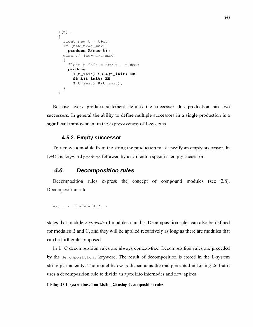
60
A(t) : { float new_t = t+dt; if (new_t<=t_max) produce A(new_t); else // (new_t>t_max) { float t_init = new_t - t_max; produce I(t_init) SB A(t_init) EB SB A(t_init) EB I(t_init) A(t_init); } }
Because every produce statement defines the successor this production has two
successors. In general the ability to define multiple successors in a single production is a
significant improvement in the expressiveness of L-systems.
4.5.2. Empty successor
To remove a module from the string the production must specify an empty successor. In
L+C the keyword produce followed by a semicolon specifies empty successor.
4.6. Decomposition rules
Decomposition rules express the concept of compound modules (see 2.8).
Decomposition rule
A() : { produce B C; }
states that module A consists of modules B and C. Decomposition rules can also be defined
for modules B and C, and they will be applied recursively as long as there are modules that
can be further decomposed.
In L+C decomposition rules are always context-free. Decomposition rules are preceded
by the decomposition: keyword. The result of decomposition is stored in the L-system
string permanently. The model below is the same as the one presented in Listing 26 but it
uses a decomposition rule to divide an apex into internodes and new apices.
Listing 28 L-system based on Listing 26 using decomposition rules

61
#define dt 0.03 #define t_max 1.0 module A(float); module I(float); axiom: A(0); derivation length: 100; p1: A(t) : { produce A(t+dt); } p2: I(t) : { produce I(t+dt); } decomposition: d1: A(t) : { if (t>t_max) { float t_init = t - t_max; produce I(t_init) SB A(t_init) EB SB A(t_init) EB I(t_init) A(t_init); } }
The decomposition rule (d1) in Listing 28 contains a condition (t>t_max), which makes
sure that apices are not decomposed infinitely by imposing a terminating condition. If a
decomposition rule does not contain a terminating condition (or if there is a bug and the
condition is never satisfied), an infinite recursion could result. To avoid infinite recursion a
safeguard parameter called maximum decomposition depth can be specified using the
following syntax:
maximum depth: expression;
If no maximum depth is specified then a default value is used. If the maximum depth is
reached during the execution of a program then a run-time warning message will be
printed.
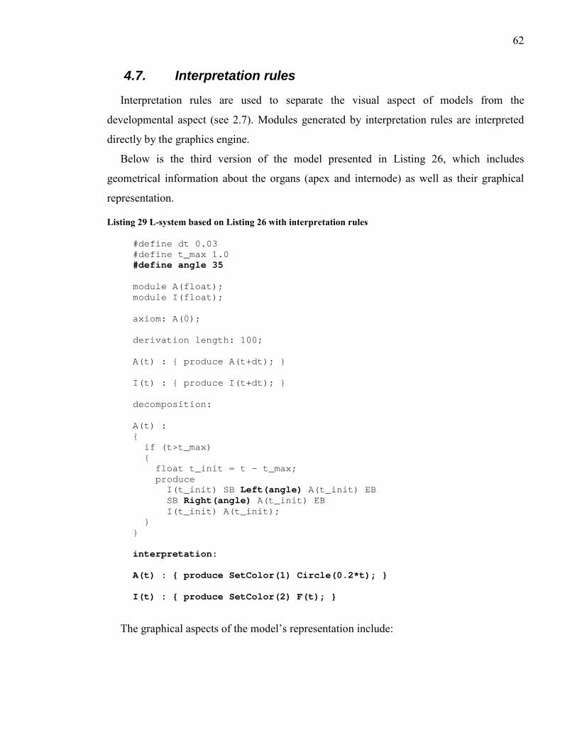
62
4.7. Interpretation rules
Interpretation rules are used to separate the visual aspect of models from the
developmental aspect (see 2.7). Modules generated by interpretation rules are interpreted
directly by the graphics engine.
Below is the third version of the model presented in Listing 26, which includes
geometrical information about the organs (apex and internode) as well as their graphical
representation.
Listing 29 L-system based on Listing 26 with interpretation rules
#define dt 0.03 #define t_max 1.0 #define angle 35 module A(float); module I(float); axiom: A(0); derivation length: 100; A(t) : { produce A(t+dt); } I(t) : { produce I(t+dt); } decomposition: A(t) : { if (t>t_max) { float t_init = t - t_max; produce I(t_init) SB Left(angle) A(t_init) EB SB Right(angle) A(t_init) EB I(t_init) A(t_init); } } interpretation: A(t) : { produce SetColor(1) Circle(0.2*t); } I(t) : { produce SetColor(2) F(t); }
The graphical aspects of the model�s representation include:

63
1) Lateral apices are orientated relative to the main branch (modules Left and Right
in the decomposition rule)
2) Interpretation rules specify that apices should be visualized as circles and internodes
as lines (module F). Apices and internodes are rendered using two different colours
(modules SetColor in the interpretation rules).
4.8. Control statements
There are four control statements in L+C: Start, StartEach, EndEach and End. Control
statements are procedures that are called at specific points of the execution of an L+C
program: at the beginning, before every derivation step, after every derivation step and after
the last step, respectively. The following sample program demonstrates how to use control
statements to output results of a simulation to an external file. This program is another
modification of the model presented in Listing 26:
Listing 30 L-system based on Listing 26 using control statements and file I/O
#define dt 0.03 #define t_max 1.0 module A(float); module I(float); axiom: A(0); derivation length: 100; int stepno, apexcount; FILE* fpOutput; Start: { fpOutput = fopen(“output.dat”, “w”); stepno = 0; } StartEach: { apexcount = 0; stepno++; } EndEach: { fprintf(fpOutput, “Step: %d\t, Number of apices: %d\n”,

64
stepno, apexcont); } End: { fclose(fpOutput); } A(t) : { float new_t = t+dt; if (t<=t_max) { apexcount++; produce A(new_t); } else // (t>t_max) { float t_init = t - t_max; apexcount += 3; produce I(t_init) SB A(t_init) EB SB A(t_init) EB I(t_init) A(t_init); } } I(t) : { produce I(t+dt); }
In addition to generating the branching structure this program also stores some statistical
information in an external file (output.dat). In the Start statement it opens the external
file output.dat and sets the stepno (step number) variable to 0. Before every derivation
step StartEach is executed where apexcount (apex counter) is set to 0 and stepno is
incremented. After every derivation step EndEach is executed which writes to the output
file current step number and the number of apices in the model. At the end of the simulation
the End statement is executed, which closes the output file.
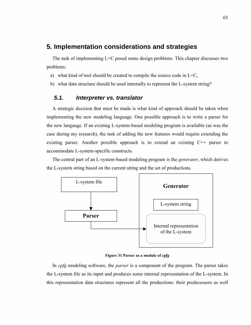
65
5. Implementation considerations and strategies The task of implementing L+C posed some design problems. This chapter discusses two
problems:
a) what kind of tool should be created to compile the source code in L+C,
b) what data structure should be used internally to represent the L-system string?
5.1. Interpreter vs. translator
A strategic decision that must be made is what kind of approach should be taken when
implementing the new modeling language. One possible approach is to write a parser for
the new language. If an existing L-system-based modeling program is available (as was the
case during my research), the task of adding the new features would require extending the
existing parser. Another possible approach is to extend an existing C++ parser to
accommodate L-system-specific constructs.
The central part of an L-system-based modeling program is the generator, which derives
the L-system string based on the current string and the set of productions.
Generator
Internal representation of the L-system
L-system file
Parser
L-system string
Figure 31 Parser as a module of cpfg
In cpfg modeling software, the parser is a component of the program. The parser takes
the L-system file as its input and produces some internal representation of the L-system. In
this representation data structures represent all the productions: their predecessors as well

66
as their code. The code (sequence of statements to be performed) is stored as a list of
structures that represent individual statements; expressions are stored as arithmetic trees
etc. In this approach the developer has the full control over the parser. But at the same time
this approach requires the developer to write parser for elements that are not typical to L-
systems but common to other programming languages: arithmetic expressions,
programming statements such as assignments, loops, conditional statements, etc. Also the
execution of interpreted code is known to be usually slow compared to compiled code.
A translator incorporates the following design:
Translation phase
Generator L-system file
Compiled executable
L-system string
Figure 32 Schematics of the new design
For practical purposes the L-system file is not compiled into a standalone program, but
into a DLL (dynamic-link library), to which a modeling program can connect at run-time.
The translation phase can be designed to consist of the following steps:
C++ compiler and linker
L+C to C++ translator (L2C)
C++ preprocessor
Preprocessed code
L+C code
Translated C++ code
Compiled executable file (DLL)

67
Figure 33 From L+C to compiled executable file, phases of translation
The second step � translating from the pre-processed L+C code to valid C++ code �is of
main interest here, because all the other steps can be accomplished using existing tools
(C++ preprocessor and compiler). The L+C to C++ translator will be also called L2C.
The main advantages of the translator approach is:
• only L+C specific elements must be identified and replaced with equivalent code in
C++,
• the translator can pass verbatim all other elements of the program to the C++
compiler,
• the compiled code can be expected to execute faster than interpreted code,
especially in domains in which the interpreted code is particularly slow (for
example, numerical calculations).
Before the specifications of the translator can be defined fully it is necessary to discuss
the problem of representing an L-system string internally.

68
5.2. L-system string representation
5.2.1. Traditional approach
Hanan [Han1992] proposed that the parametric L-system string be represented verbatim.
In general a module with numerical parameters is stored internally in the form presented in
Figure 34.
One module with parameters
More float parameters
A ( , ) B
sizeof(float)
Figure 34 Traditional memory representation of L-system string
In Figure 34, every frame represents one byte. To represent a module A with some
numerical parameters the first byte will be letter A (or actually the number that corresponds
to the letter A in ASCII code). The next byte contains the left (opening) parenthesis. The
actual parameters are stored as their binary representation in the following bytes. If the
numerical parameters are of type float stored in the IEEE format they occupy four bytes (or
in general sizeof(float) bytes). Consecutive parameters are separated with bytes
containing comma �,�. The last parameter is followed by the right (closing) parenthesis. If
a module doesn�t have any parameters then its symbol is immediately followed by the next
module. In addition it is assumed that the last module is followed by the null character and
that the pointer to the beginning of the string is known.
To perform string derivation it is necessary to iterate forward and backward through the
string � find the next and the previous module (if there is one).
The internal representation described above allows such iterations (for the actual listings
see B.1). Figure 35 presents the corresponding algorithms:

69
no
no
yes
yes
Start
�(� found?
Skip sizeof(float)+1 forward
�,� found?
Skip one byte forward
Skip one byte forward
Next module found
no
no
yes
yes
Start
�)� found?
Skip sizeof(float)+1 back
�,� found?
Skip one byte back
Skip one byte back
Previous module found
Figure 35 Algorithms to find the next and previous module for the traditional string representation
An important question is whether this representation can be extended to support modules
that have parameters of user-defined types. A naïve approach could be to store user-defined
type parameters in the same way as implemented previously:
Any number of bytes
A ( , ) B
Any number of bytes
One module with parameters
,
Figure 36 New L-system string memory representation, attempt one
When trying to formulate algorithms for iterating the string the following problems
arise:
1. The size of parameters is not fixed. Parameters can be of arbitrary type, so they can
also be of arbitrary size. Therefore it is impossible to skip a parameter forward to
check whether it is followed by a comma (indicating presence of another parameter

70
following the comma) or the closing parenthesis. This problem might be addressed
if the sizes of parameters for a given module are known.
2. When iterating backwards (searching for the beginning of the previous module)
information about the sizes of parameters is not enough for two reasons. First, the
size information is not available until the module has been identified. Second, a
module cannot be identified until the parameters have been skipped to read its
name.
5.2.2. Proposed solution
Module id as short int
Module id as short int
0x12 0xAB
One module with parameters
Binary representation of the module�s parameters
0x12 0xAB 0xE1 0x2B
Figure 37 New L-system string memory representation
The proposed solution is presented in Figure 37. The main differences between the
previous and new representation are:
1. the module�s name is encoded as a fixed size identifier. Here it is assumed to be a C
short int � an integral type stored in two bytes,
2. the identifier is present at both the beginning and end of the module,
3. parameters are not comma separated. They occupy a continuous region of memory,
4. if a module does not have any parameters it is represented as its identifier of type
short int,
5. the format does not provide an end-of-string character. Information about the total
length is stored separately.
With this representation the string can be iterated both forward and backward if access
to the total size of parameters for every module type is provided.
Listing 46 and Listing 47 in appendix B contain the code that moves the current pointer
in the L-system string to the next and previous module. The code in Listing 46 and Listing
47 refers to function GetParametersSize. This function is part of the interface that

71
communicates between the dynamic part of the program (L-system) and fixed generator.
This interface defines how the generator manipulates the string, what code should be
generated by the L+C to C++ translator and how this code should cooperate with the
generator. The interface is presented in the next chapter.

72
6. The L+C to C++ translator When designing the translator it is crucial to identify its top-level requirements:
1. the translator must generate valid C++ code
2. the code generated by the translator must conform to guidelines that allow for the
generator to access the information required to perform production matching as well
as other information specific to L-systems (derivation length, axiom, etc.)
The first requirement is obvious and requires no further explanation. The second
requirement demands that some sort of interface be defined to link the translated (and
compiled) L+C program with the generator.
The L+C translator divides its input (code in L+C) into three categories (see Figure 38):
1. Code that needs to be translated,
2. Code that requires additional code to be generated (bridge code),
3. C++ code that is not modified and passed verbatim to the C++ compiler. L+C
Translated code
Bridge data and code
L-system engine (generator)
Unmodified C++ code
L+C to C++ translator
Compiled DLL C++
compiler
Figure 38 Relation between the components: code in L+C, L-system generator and compiled DLL.
The elements of an L+C program that are specific to L-systems and need to be translated
are:
1. Global L-system parameters (derivation length, maximum decomposition depth,
maximum interpretation depth),
2. Axiom,
3. Control statements,
4. Definitions of modules,

73
5. Productions,
6. Consider/ignore statements.
Figure 39 presents a sample code in L+C. Translation units belonging to different
categories are highlighted. The following sections discuss in more detail how different
statements are translated into C++ code.
L+C code
Intact code
module A(int, float); module B(float, ModuleData);
axiom: A(1, 0.5);
derivation length: 5;
void Func(float, int* ) { … }
A(n, f) < B(f, d) : { if (n>0) produce B(f/2, d); else produce A(n, f*1.5); }
class ModuleData { public: ModuleData(); … private: int n; float x; … };
C++ data declarations
C++ functions
Intact code
C++ function prototypes.
Bridge code (production callers)
Bridge data (callers table)
C++ function calls
Products of translation
Figure 39 Sample source code in L+C, L+C to C++ translation units
The following sections identify different elements of programs written in L+C and
explain how they are translated by the L2C translator and then used by lpfg.

74
6.1. Top level parameters and statements
This Execute function is the core of the generator component of lpfg.
Listing 31 Function executing L+C program
void Execute() { Start(); Axiom(); DecomposeString(MaximumDecompositionDepth()); for (int i=0; i<DerivationLength(); ++i) { StartEach(); Derive(); DecomposeString(MaximumDecompositionDepth()); EndEach(); } End(); }
This simplified code refers to functions, highlighted in bold, that are not part of the
generator. These functions are created by the L2C translator and provide information from
the L-system or perform actions specified in the L-system.
• Start() executes the Start control statement,
• Axiom() initializes the L-system string ,
• MaximumDecompositionDepth() returns the value of an expression that specifies
maximum decomposition depth in the L-system,
• DerivationLength() returns the value of an expression that specifies the number
of derivation steps to be performed as specified in the L-system,
• StartEach() executes the StartEach control statement,
• EndEach() executes the EndEach control statement,
• End() executes the End control statement.
The following sections discuss how these functions are created during translation from
L+C to C++.
6.2. L-system global parameters
Every program in L+C defines the following numeric parameters:

75
• Derivation length
• Maximum decomposition depth
• Maximum interpretation depth
These parameters are always defined. If they are not specified explicitly (maximum
decomposition and interpretation depth are optional), then the translator provides default
values. These global parameters are integers. They are accessible to the generator through
functions. The prototypes of the functions are:
int DerivationLength();
int MaximumDecompositionDepth();
int MaximumInterpretationDepth();
Each of the three global parameters (derivation length, maximum decomposition and
interpretation depth) is specified in the L+C file by a keyword (derivation length,
maximum depth) followed by an arithmetic expression and terminated with a semicolon.
The translator replaces the keyword with a C++ function prototype. The expression is
copied verbatim and the closing (right) curly brace is appended. Here the replaced elements
are printed in boldface while the elements copied verbatim are in italic.
Original code: Translated code: derivation length: i+3; int DerivationLength() { return i+3; }
Analogous substitutions are done in case of maximum decomposition and interpretation
depth.
6.3. L-system control statements
L-system control statements are statements that are executed at specific points of the
simulation, and they are: Start, End, StartEach, EndEach. These statements are actually
procedures without parameters. In C++ such procedures are functions that take no

76
parameters and return void. Because the body of the control statements can contain any
valid C++ code, the L2C translator must only replace control statement keywords with C++
function prototypes to create a valid C++ function definition:
Original code: Translated code: Start: { … }
void Start() { … }
Analogous substitutions are made for the other control statements.
6.4. Module declaration
A module declaration contains two pieces of information: the name of the module and
the parameters� types. The code in Listing 31 does not use any of this information
explicitly. From the discussion on the internal representation of the L-system string (see
section 5.2) it is known that information about the total size of the parameters is required to
iterate over the string and carry out the derivation. From the same discussion it is also
known that the modules in the string are not identified by their names, but by numerical
identifiers. The L2C translator replaces module declarations with the declarations of
module identifiers:
Original code: Translated code: module A(int, float); short int A_id = 101;
The identifier name is created by appending _id to the module�s name. The identifiers�
values are consecutive integers.
This substitution does not contain information about the size of parameters of the
module. Instead, size information is stored in an array, which is generated after the L+C
source file has been parsed:
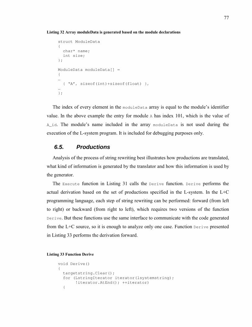
77
Listing 32 Array moduleData is generated based on the module declarations
struct ModuleData { char* name; int size; }; ModuleData moduleData[] = { … { “A”, sizeof(int)+sizeof(float) }, … };
The index of every element in the moduleData array is equal to the module�s identifier
value. In the above example the entry for module A has index 101, which is the value of
A_id. The module�s name included in the array moduleData is not used during the
execution of the L-system program. It is included for debugging purposes only.
6.5. Productions
Analysis of the process of string rewriting best illustrates how productions are translated,
what kind of information is generated by the translator and how this information is used by
the generator.
The Execute function in Listing 31 calls the Derive function. Derive performs the
actual derivation based on the set of productions specified in the L-system. In the L+C
programming language, each step of string rewriting can be performed: forward (from left
to right) or backward (from right to left), which requires two versions of the function
Derive. But these functions use the same interface to communicate with the code generated
from the L+C source, so it is enough to analyze only one case. Function Derive presented
in Listing 33 performs the derivation forward.
Listing 33 Function Derive
void Derive() { targetstring.Clear(); for (LstringIterator iterator(lsystemstring); !iterator.AtEnd(); ++iterator) {
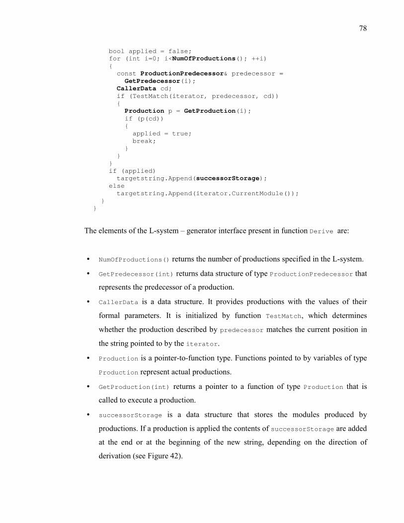
78
bool applied = false; for (int i=0; i<NumOfProductions(); ++i) { const ProductionPredecessor& predecessor = GetPredecessor(i); CallerData cd; if (TestMatch(iterator, predecessor, cd)) { Production p = GetProduction(i); if (p(cd)) { applied = true; break; } } } if (applied) targetstring.Append(successorStorage); else targetstring.Append(iterator.CurrentModule()); } }
The elements of the L-system � generator interface present in function Derive are:
• NumOfProductions() returns the number of productions specified in the L-system.
• GetPredecessor(int) returns data structure of type ProductionPredecessor that
represents the predecessor of a production.
• CallerData is a data structure. It provides productions with the values of their
formal parameters. It is initialized by function TestMatch, which determines
whether the production described by predecessor matches the current position in
the string pointed to by the iterator.
• Production is a pointer-to-function type. Functions pointed to by variables of type
Production represent actual productions.
• GetProduction(int) returns a pointer to a function of type Production that is
called to execute a production.
• successorStorage is a data structure that stores the modules produced by
productions. If a production is applied the contents of successorStorage are added
at the end or at the beginning of the new string, depending on the direction of
derivation (see Figure 42).

79
Below is a detailed description of the interface elements present in Listing 33.
NumOfProductions
Function int NumOfProductions() is generated by L2C after the source file has been
parsed. As the translator parses the L+C program it counts the number of productions and
can generate the function:
int NumOfProductions() { return 7; }
ProductionPredecessor, GetPredecessor
Before the structure ProductionPredecessor can be defined it is necessary to identify
what information is necessary to determine if a given production matches the current
module. Matching a production requires a comparison of modules in the string and modules
in the production�s predecessor. The modules in the string are identified by numbers (see
section 5.2). This means that a production�s predecessor is fully defined by three sets of
module identifiers: one set each for left context, the strict predecessor and the right context.
struct ProductionModules { short int module_ids[maxModules]; int count; }; struct ProductionPredecessor { ProductionModules lcntxt; ProductionModules strict; ProductionModules rcntxt; };
L2C translator generates an array of structures of type ProductionPredecessor.
Elements of this array are returned by the function GetPredecessor(int).
For example, if a program contains a production with the following predecessor:
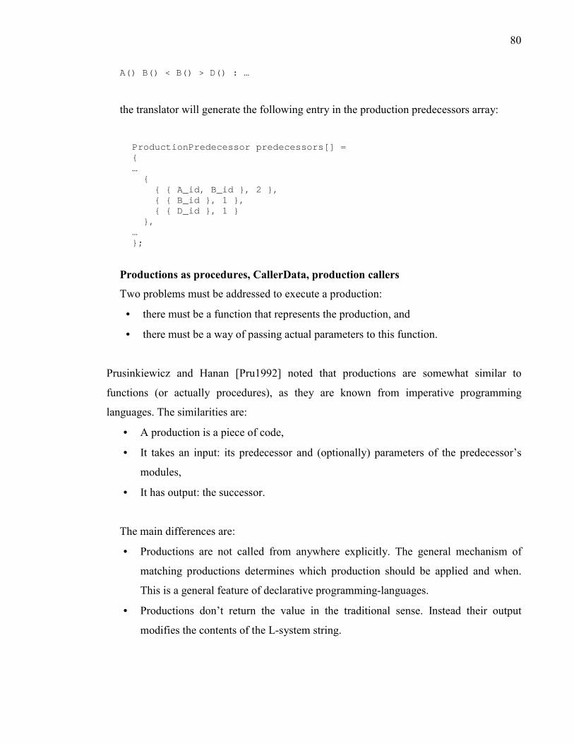
80
A() B() < B() > D() : …
the translator will generate the following entry in the production predecessors array:
ProductionPredecessor predecessors[] = { … { { { A_id, B_id }, 2 }, { { B_id }, 1 }, { { D_id }, 1 } }, … };
Productions as procedures, CallerData, production callers
Two problems must be addressed to execute a production:
• there must be a function that represents the production, and
• there must be a way of passing actual parameters to this function.
Prusinkiewicz and Hanan [Pru1992] noted that productions are somewhat similar to
functions (or actually procedures), as they are known from imperative programming
languages. The similarities are:
• A production is a piece of code,
• It takes an input: its predecessor and (optionally) parameters of the predecessor�s
modules,
• It has output: the successor.
The main differences are:
• Productions are not called from anywhere explicitly. The general mechanism of
matching productions determines which production should be applied and when.
This is a general feature of declarative programming-languages.
• Productions don�t return the value in the traditional sense. Instead their output
modifies the contents of the L-system string.

81
Consider the following example (elements specific to L+C have been highlighted with
boldface):
Listing 34 Sample production with multiple successors
struct data { float l; int n; }; module A(data, float); module B(int, float); A(dl, xl) < B(n, a) : { float x = f(n, dl.l); if (a>xl) produce B(n+1, x); else produce B(n-1, xl); }
The production in Listing 34 has two modules in its predecessor. The first line of this
production will be regarded as corresponding to the C++ function prototype. A function
prototype contains the following elements:
• name,
• parameters,
• return type.
In L-systems there is no return type of productions, because they don�t return values. In
C++ the function name and parameters identify the function. In L-systems, on the other
hand, the names of the modules in the predecessor (and the order of their appearance in all
the three parts of the predecessor: left context, strict predecessor and right context) identify
a production. The parameters are implicit, the modules have to be declared beforehand.
A production predecessor is a distinctive element of L+C. On one hand, it identifies the
part of the string that is to be replaced (the strict predecessor) and optionally the context �
the neighbour modules of the strict predecessor. On the other hand, the production
predecessor corresponds to a procedure (or function) prototype: it specifies the input
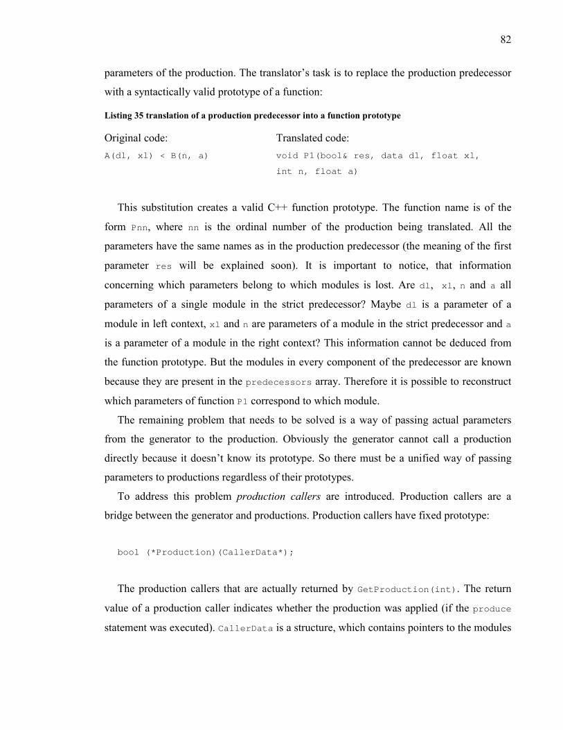
82
parameters of the production. The translator�s task is to replace the production predecessor
with a syntactically valid prototype of a function:
Listing 35 translation of a production predecessor into a function prototype
Original code: Translated code: A(dl, xl) < B(n, a) void P1(bool& res, data dl, float xl,
int n, float a)
This substitution creates a valid C++ function prototype. The function name is of the
form Pnn, where nn is the ordinal number of the production being translated. All the
parameters have the same names as in the production predecessor (the meaning of the first
parameter res will be explained soon). It is important to notice, that information
concerning which parameters belong to which modules is lost. Are dl, xl, n and a all
parameters of a single module in the strict predecessor? Maybe dl is a parameter of a
module in left context, xl and n are parameters of a module in the strict predecessor and a
is a parameter of a module in the right context? This information cannot be deduced from
the function prototype. But the modules in every component of the predecessor are known
because they are present in the predecessors array. Therefore it is possible to reconstruct
which parameters of function P1 correspond to which module.
The remaining problem that needs to be solved is a way of passing actual parameters
from the generator to the production. Obviously the generator cannot call a production
directly because it doesn�t know its prototype. So there must be a unified way of passing
parameters to productions regardless of their prototypes.
To address this problem production callers are introduced. Production callers are a
bridge between the generator and productions. Production callers have fixed prototype:
bool (*Production)(CallerData*);
The production callers that are actually returned by GetProduction(int). The return
value of a production caller indicates whether the production was applied (if the produce
statement was executed). CallerData is a structure, which contains pointers to the modules

83
in the string being rewritten (see Figure 40). TestMatch initializes CallerData while
determining whether a given production matches the current position in the string.
Production callers are functions generated by the translator and their responsibility is to
extract the parameters from the string and pass them to the actual production. Production
callers also inform the generator whether the production was applied. A sample production
caller corresponding to the production from Listing 35 looks as follows:
Listing 36 Sample production caller
bool PC1(CallerData* pCD) { // extract parameters for the left context data dl; const char* pX = pCD->lcntxt.Addr[0]; // first data memcpy(&dl, pX, sizeof(data)); // skip sizeof(data) bytes pX += sizeof(data); float xl; // and extract a float memcpy(&xl, pX, sizeof(float); // now extract parameters for the strict predecessor int n; pX = pCD->strict.Addr[0]; memcpy(&n, pX, sizeof(int)); pX += sizeof(int); float a; memcpy(&a, pX, sizeof(float)); // if there were any modules in the right predecessor // the parameters would be extracted here bool res = false; // assume that the production did not apply // call the production-function P1(res, dl, xl, n, a); return res; }

84
Current module
CallerData
Strict predecessor Left context Right context
String
Pointers to modules in left
context
Pointers to modules in strict
predecessor
Pointers to modules in right
context
� � �
Figure 40 CallerData makes it possible to access a production�s actual parameters
A_id A_id Y_id Y_id I_id Z_id Z_id 1 2 0.5
CallerData { … strict { … }, count = 1;
rcntxt { …}, count = 2;
}
String
Figure 41 Mapping parameters locations into a CallerData structure
The actual definition of CallerData is as follows:
struct ActualParameters { char* Addr[MaxParameters];
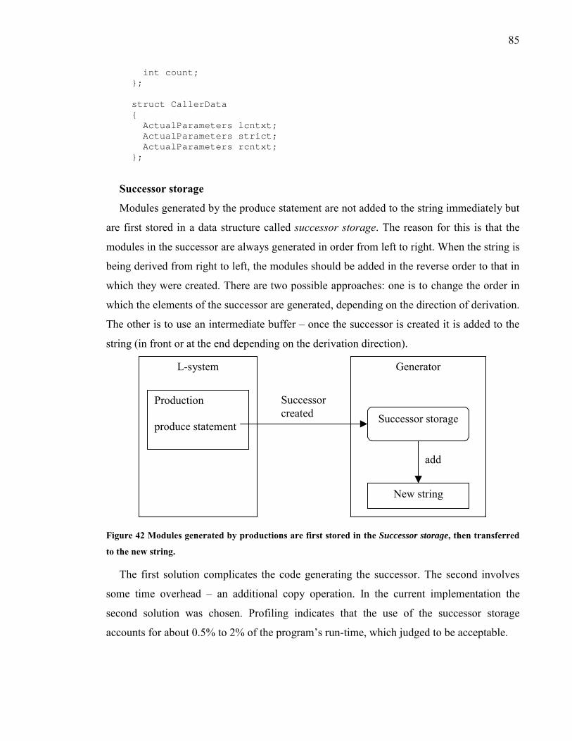
85
int count; }; struct CallerData { ActualParameters lcntxt; ActualParameters strict; ActualParameters rcntxt; };
Successor storage
Modules generated by the produce statement are not added to the string immediately but
are first stored in a data structure called successor storage. The reason for this is that the
modules in the successor are always generated in order from left to right. When the string is
being derived from right to left, the modules should be added in the reverse order to that in
which they were created. There are two possible approaches: one is to change the order in
which the elements of the successor are generated, depending on the direction of derivation.
The other is to use an intermediate buffer � once the successor is created it is added to the
string (in front or at the end depending on the derivation direction).
Generator
add
L-system
Production produce statement
Successor storage
Successor created
New string
Figure 42 Modules generated by productions are first stored in the Successor storage, then transferred
to the new string.
The first solution complicates the code generating the successor. The second involves
some time overhead � an additional copy operation. In the current implementation the
second solution was chosen. Profiling indicates that the use of the successor storage
accounts for about 0.5% to 2% of the program�s run-time, which judged to be acceptable.
86
6.6. The produce statement
The produce statement plays two roles, specifying the successor of the production, and
implying that the execution of the production should terminate (return statement)10. While
building a successor, the DLL generated from the L+C source file needs to modify data that
belongs to the main program.
SuccessorStorage is the data structure where the successor is created by a production.
After the production is applied, the complete successor is added to the string. The generator
has to provide a function that will let the DLL (or the productions to be exact) add data to
the SuccessorStorage. This function is called Add:
void Add(const void*, int);
The first parameter is a pointer to the data to be added and the second parameter is the
number of bytes to be added. The code calling Add takes full responsibility that the data
stored in the SuccessorStorage are correct, e.g. it follows the specifications of the L-
system string. If the data to be added are contained in variables, the Add function could be
used directly:
Add(&B_id, sizeof(short int)); Add(&n, sizeof(int)); Add(&x, sizeof(float)); Add(&B_id, sizeof(short int));
But in general this is not the case. Both produce statements in Listing 34 generate
modules with their parameters specified using expressions. C++ does not allow one to
obtain the address of an expression. Consequently the following construct is not valid in
C++:
10 The two functions could be split, so that the keyword produce just produced the successor, but did not
terminate the production. Alternatively another keyword (for example insert) could be introduced to
generate the successor, but not terminating the production, making it possible to build the successor in a series
of insert statements. This idea seems worth considering in the future research.

87
Add(&(n+1), sizeof(int));
One possible solution is to declare local variables that store the values of parameters and
use them in the call to Add:
Add(&B_id, sizeof(short int)); int n1 = n+1; Add(&n1, sizeof(int)); Add(&x, sizeof(float)); Add(&B_id, sizeof(short int));
This approach is acceptable but would complicate the implementation of the L+C parser.
A more effective and general solution has been chosen. A template function
Produce is defined as follows: template<class T> void Produce(T t) { Add(&t, sizeof(T)); }
Now the translation of the produce statement is straightforward: Produce<short int>(B_id); Produce<int>(n+1); Produce<float>(x); Produce<short int>(B_id);
This solution takes advantage of the C++ compiler�s optimizing capabilities and greatly
simplifies both the L+C parser and the generated code. Note the explicit types in the
instantiation of Produce, so that the type used is the same as the type of the parameter
being produced. Otherwise the C++ compiler could perform an implicit type conversion
and generate Add for a wrong type. For example, it is common to use a literal like 1 where a
float is expected instead of 1.0f. But in this case the compiler would assume that <int>
instance is required. This kind of mistake could result in a corrupted string.
Finally, the production caller must be informed if the production was actually applied.
This is done by assigning true to the parameter res (see Listing 35 and Listing 36). Finally
all the code generated in place of the produce statement is enclosed in curly braces, so that
it actually forms a single (compound) statement: { Produce<short int>(B_id);

88
Produce<int>(n+1); Produce<float>( x); Produce<short int>(B_id); res = true; return; }
6.7. Other elements
6.7.1. Ignore, consider
The ignore and consider statements are mutually exclusive. Each of these statements
is replaced by a declaration of an array of module identifiers and a function that returns the
number of elements in the array. For example:
Original code: Translated code: ignore: A B Left Right; short int ignored[] =
{ A_id, B_id, Left_id, Right_id }; int NumOfIgnored() { return 4; }
6.7.2. Axiom
Axiom is a special type of production that does not have a predecessor. It is replaced by
a function named Axiom. Contents of the axiom are expanded as if it were a produce
statement. This function can be called directly by the generator.
Original code: Translated code: Axiom: F(1) Left(90) F(1); void Axiom()
{ Produce<short int>(F_id); Produce<float>(1); Produce<short int>(F_id); … }
6.7.3. Production, decomposition, interpretation
These keywords are not actually translated. Instead, they change the internal state of the
translator that determines the allowed types of the productions (if context-sensitive
productions are allowed). Also, in the case of decomposition and interpretation rules there
is no array of ProductionPredecessor. Instead there are two arrays of ProdCallers: one
for interpretation and one for decomposition rules.
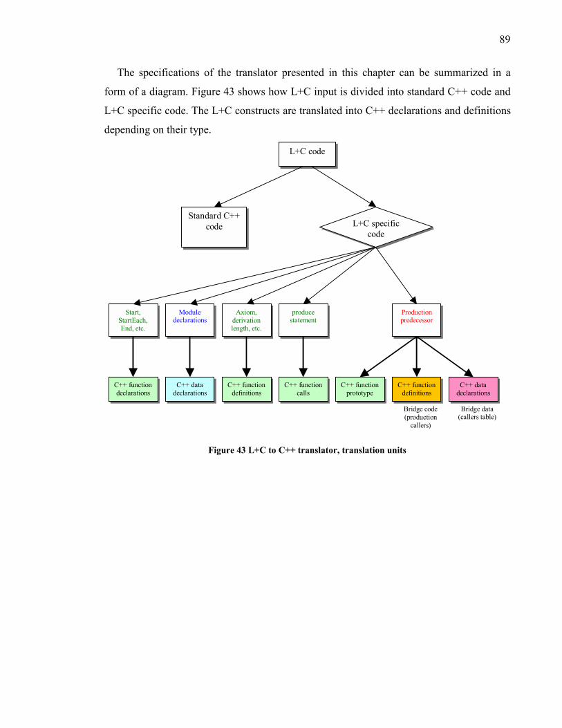
89
The specifications of the translator presented in this chapter can be summarized in a
form of a diagram. Figure 43 shows how L+C input is divided into standard C++ code and
L+C specific code. The L+C constructs are translated into C++ declarations and definitions
depending on their type.
Bridge data (callers table)
Bridge code (production
callers)
C++ function declarations
C++ data declarations
C++ function definitions
C++ function calls
C++ function prototype
C++ function definitions
C++ data declarations
Production predecessor
produce statement
Axiom, derivation length, etc.
Module declarations
Start, StartEach, End, etc.
L+C specific code
Standard C++ code
L+C code
Figure 43 L+C to C++ translator, translation units
90
7. Application examples This section presents examples that demonstrate the use of the L+C modeling language.
They have been selected to demonstrate the use of concepts and features introduced in
L+C.
7.1. Model of Anabaena
This example implements a developmental model of a filamentous cyanobacterium
Anabaena catenula. The distribution of heterocysts (term described below) in the filament
tends to form a pattern. The model captures this tendency by operating on genes�
expression: production of two proteins. This model extends the model presented in Listing
1 in section 2.1 and was written by P. Prusinkiewicz (unpublished). It employs user-defined
structures to store the parameters that describe cells and user-defined functions to perform
calculations.
In the model presented in Listing 37, the cells are characterized by the following
parameters:
• Concentration of protein hetR,
• Concentration of protein patS,
• Length,
• Polarity,
• Differentiation degree.
Initially the model consists of two cells. During the simulation the concentration of the
activator hetR and inhibitor patS controls cell development. The concentration changes as
the result of the following processes:
1. diffusion of patS (transfer of the substance from a cell of high concentration to cells
of lower concentration),
2. production,
3. decay.

91
Diffusion
The change of concentration caused by diffusion of patS from a cell of size x over the
time increment ∆t is expressed by formula:
txw
patSpatSDpatSdiff ∆
−=∆ 2 ,
where D is diffusion constant, w is the width of the cell, and patS2 is the concentration in
the neighbouring cell. If the concentration in the current cell is greater than that in the other
cell, then the substance will diffuse to the other cell and the concentration will decrease (the
numerator patS2-patS is negative). If the concentration in the current cell is lower it will
increase.
If the current cell has two adjacent neighbours (labelled l and r), diffusion equals the
sum of the diffusions between the cell and both of its neighbours. Diffusion is then
expressed by formula:
txw
patSpatSpatSDpatS rldiff ∆
−+=∆
2
Production
The amount of patS produced in the time interval ∆t depends on the concentration of
hetR in the cell. It is expressed by the formula
xth
hetRhetRpatS prod
∆
+
⋅+=∆ 02
2
1 κρ ,
where ρ, κ and h0 are parameters, x is the size of the cell. HetR acts as the activator.
The amount of hetR during the time interval ∆t depends on the concentration of both
hetR and patS. HetR is an activator and patS is an inhibitor as expressed by the formula
below:

92
xta
hetRhetR
patShetR ∆
+
⋅+=∆ 02
2
1 κρ
If the concentration of hetR exceeds a threshold, the cell becomes a heterocyst.
Heterocysts do not divide.
Decay
The decay of proteins during ∆t is expressed by the following formulas:
thetRhetR ∆−=∆ µ tpatSpatS ∆−=∆ ν ,
where µ and ν are decay parameters. Decay is implemented in the decomposition rule d1.
Growth and division
During every time step cells grow in length (decomposition rule d1), resulting in
decreased concentration of hetR and patS. Cells grow during the simulation and divide
(except for heterocysts) if their size exceeds a threshold. Polarity of the cells determines
which of the daughter cells is longer.
Implementation of the model
Modules of type Cell represent cells. The information associated with every cell is
stored in the Cell parameter of type CellData.
Diffusion is controlled by productions p1, p2 and p3. p2 and p3 apply when a cell has only
one neighbour. During the derivation, diffusion of patS is calculated. The successors of the
productions are modules of type TempCell, to distinguish between the cells before and after
the growth phase handled by decomposition. This distinction avoids infinite recursion in
the decomposition rules.
The growth phase of the simulation (decomposition d1) involves three stages. First, the
new concentrations of both patS and hetR are determined as a result of their production by
the cell using the HetR and PatS functions. Then the decay of the substances is calculated.
93
Finally, the cells grow and those that reach the maximum size and are not heterocysts
divide.
Listing 37 Model of Anabaena in L+C
enum Polarity { plRight, plLeft }; // daughter cell length coefficients const float longer = 0.55f; const float shorter = 1.0f - longer; const float rho = 3; // protein production parameter const float a0 = 0.01; // base activator production const float h0 = 1; // base inhibitor production const float mu = 0.1; // hetR decay rate const float nu = 0.45; // patS decay rate const float D_patS = 0.0045; // diffusion coefficient const float kappa = 0.001; // protein production coefficient const float dt = 0.5; // time step const float w = 0.01; // diffusion w parameter const float lm = 1.0; // cell maximum size const float gr = 1.002; // growth rate of cells const float thr = 0.5; // treshold hetR value for heterocysts struct CellData { float hetR, patS; // protein concentrations float x; // cell size (length) Polarity p; // plLeft or plRight float vph; // differentiation degree // vegetative-pro-hetero }; // Definition of modules used in the model module Cell(CellData); module TempCell(CellData); // Production of proteins float HetR(float hetR, float patS) { return rho/patS*(hetR*hetR/(1+kappa*hetR*hetR) + a0); } float PatS(float hetR) { return rho*(hetR*hetR/(1+kappa*hetR*hetR) + h0); } // Parameters of the initial two cells CellData icd1, icd2;

94
Start: { icd1.hetR = 0.1; icd1.patS = 100.0; icd1.x = longer; icd1.p = plRight; icd1.vph = 0; icd2 = icd1; icd2.x = shorter; } Axiom: Right(90) Cell(icd1)Cell(icd2); // Interaction between cells (diffusion of patS) p1: Cell(cdl) < Cell(cd) > Cell(cdr) : { cd.patS += (D_patS*(cdl.patS+cdr.patS-2*cd.patS)/(cd.x*w))*dt; produce TempCell(cd); } p2: Cell(cd) > Cell(cdr) : { cd.patS += (D_patS*(cdr.patS-cd.patS)/(cd.x*w))*dt; produce TempCell(cd); } p3: Cell(cdl) < Cell(cd) : { cd.patS += (D_patS*(cdl.patS-cd.patS)/(cd.x*w))*dt; produce TempCell(cd); } decomposition: d1: TempCell(tcd) : { CellData cd = tcd; // Proteins production cd.hetR += HetR(tcd.hetR,tcd.patS)*dt/cd.x; cd.patS += PatS(tcd.hetR)*dt/cd.x; // Decay of proteins cd.hetR -= mu*tcd.hetR*dt; cd.patS -= nu*tcd.patS*dt; // If did not reach max size, grow if(cd.x < lm) { cd.hetR /= gr; cd.patS /= gr; cd.x *= gr; // differentiation degree of heterocyst

95
// is identified with its size if(cd.hetR>thr) cd.vph=cd.x; } // If maximum size not reached, or heterocyst, that's it if (cd.x<lm || cd.hetR>thr) produce Cell(cd); // otherwise, divide else { CellData cd1 = cd; CellData cd2 = cd; cd1.p = plLeft; cd2.p = plRight; // take polarity into account if (cd.p==plRight) { cd1.x *= longer; cd2.x *= shorter; } else { cd1.x *= shorter; cd2.x *= longer; } produce Cell(cd1) Cell(cd2); } } interpretation: // Display the cell i1: Cell(cd) : { float width; width = max(shorter, cd.vph); produce SetWidth(width) f(width/2) Circle(width/2)F((cd.x-width)/2) SB() Right(90) SetColor(2) SetWidth(shorter/4)F(log(cd.patS)) EB() SB() Left(90) SetColor(3) SetWidth(shorter/4)F(log(1000*cd.hetR)) EB() F((cd.x-width)/2)Circle(width/2)f(width/2); }
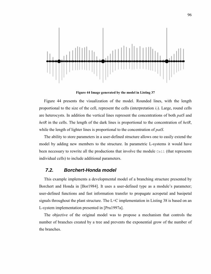
96
Figure 44 Image generated by the model in Listing 37
Figure 44 presents the visualization of the model. Rounded lines, with the length
proportional to the size of the cell, represent the cells (interpretation i1). Large, round cells
are heterocysts. In addition the vertical lines represent the concentrations of both patS and
hetR in the cells. The length of the dark lines is proportional to the concentration of hetR,
while the length of lighter lines is proportional to the concentration of patS.
The ability to store parameters in a user-defined structure allows one to easily extend the
model by adding new members to the structure. In parametric L-systems it would have
been necessary to rewrite all the productions that involve the module Cell (that represents
individual cells) to include additional parameters.
7.2. Borchert-Honda model
This example implements a developmental model of a branching structure presented by
Borchert and Honda in [Bor1984]. It uses a user-defined type as a module�s parameter;
user-defined functions and fast information transfer to propagate acropetal and basipetal
signals throughout the plant structure. The L+C implementation in Listing 38 is based on an
L-system implementation presented in [Pru1997a].
The objective of the original model was to propose a mechanism that controls the
number of branches created by a tree and prevents the exponential grow of the number of
the branches.

97
The program operates on three types of modules: apices A, internodes I and an auxiliary
module N. Each internode has a parameter of type InternodeData. InternodeData is a
structure type that contains the following fields: segment type (st), flux value (flux) and
apex count (count).
In this model, plant development is controlled by the amount of substances that
propagate acropetally (from the base of the structure towards the apices). The process of
development is modeled in discrete time steps. The development starts with a single
internode and an apex. This internode is called the base of the tree. Development of the
plant depends on the flux (flow of substances) available for every apex in the plant. At the
beginning of the simulation the base of the tree contains the initial concentration of growth
substances.
Each time step is divided into three phases. Each phase corresponds to a derivation step.
Variable stepType of type PhaseType controls the current phase. Its value is changed at
the beginning of every derivation step (StartEach statement) and cyclically assumes
values BSP (basipetal signal phase � counting apices), ASP (acropetal signal phase �
distributing flux) and GP (growth phase).
Growth phase
The age of the base is incremented (production p1). The amount of growth substances
available for every apex is checked. If this amount exceeds a threshold, the apex produces
two new branches: main and lateral (production p2).
Basipetal signal phase
During this phase the derivation is performed backward (see StartEach statement). The
number of apices supported by each internode is calculated (production p3). This includes
the apex following the internode in question or apices supported indirectly by the daughter
branches of the internode. The number of apices supported by internodes is considered an
acropetal signal and is transferred using fast information transfer.
98
Acropetal signal phase
In this phase the derivation is performed forward (see StartEach statement). The
amount of flux available for all internodes is determined. At the base the flux is calculated
(production p4) using the formula proposed by Borchert and Honda: ( ) kkv ησ 10 2 −= (see
function BaseFlux). This formula simulates a sigmoidal increase of flux over time. Starting
from the base internode, the flux is divided between the daughter branches (production p5).
The amount of flux available for a daughter internode depends on the number of apices
supported by the branch. Main branches are preferred over lateral branches in the sense that
they are assigned more flux. If two branches support the same number of apices then the
main branch is assigned λ (constant lambda) of the flux reaching the branching point and
the lateral branch obtains the remainder (1- λ) of flux. If the number of apices supported by
the main and lateral branch is different, then the flux reaching the lateral branch is
multiplied by the ratio c/cs, where c is the number of apices supported by the lateral branch
and cs is the number of apices supported by the main branch. The fraction of flux available
for a branch is calculated in the function Flux.
Listing 38 Borchert-Honda model implemented in L+C using fast information transfer
#include <math.h> // required for pow #include <lpfgall.h> // predefined modules and data structures const float Alpha1 = 10.0f; // branching angle - main segments const float Alpha2 = 32.0f; // branching angle - lateral segments const float sigma0 = 17.0f; // initial flux const float eta = 0.89f; // input flux change parameter const float vth = 5.0f; // threshold flux for branching const float lambda = 0.7f; // flux distribution factor derivation length: 36; int StepNo; // Step number counter enum PhaseType { BSP = 0, ASP, GP }; PhaseType steptype; enum SegType { stBase, stStr, stLat }; struct InternodeData { SegType st;
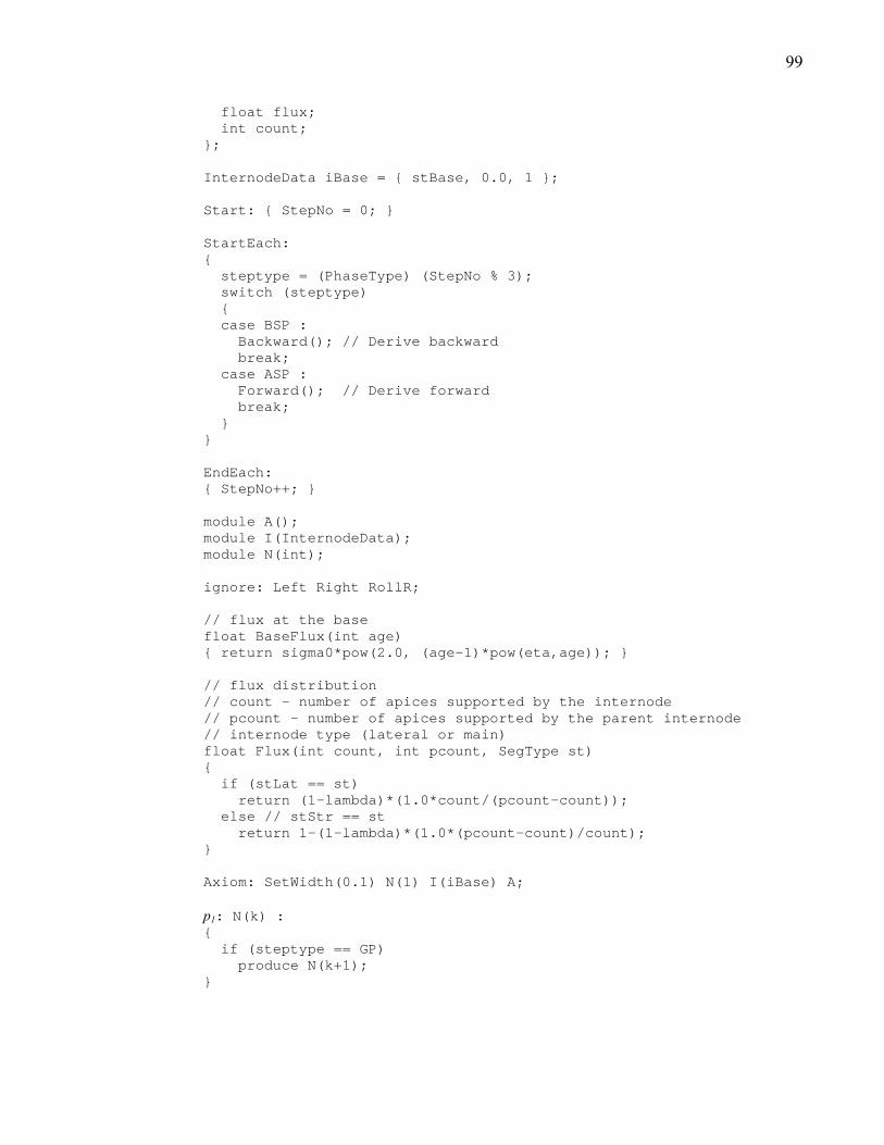
99
float flux; int count; }; InternodeData iBase = { stBase, 0.0, 1 }; Start: { StepNo = 0; } StartEach: { steptype = (PhaseType) (StepNo % 3); switch (steptype) { case BSP : Backward(); // Derive backward break; case ASP : Forward(); // Derive forward break; } } EndEach: { StepNo++; } module A(); module I(InternodeData); module N(int); ignore: Left Right RollR; // flux at the base float BaseFlux(int age) { return sigma0*pow(2.0, (age-1)*pow(eta,age)); } // flux distribution // count – number of apices supported by the internode // pcount – number of apices supported by the parent internode // internode type (lateral or main) float Flux(int count, int pcount, SegType st) { if (stLat == st) return (1-lambda)*(1.0*count/(pcount-count)); else // stStr == st return 1-(1-lambda)*(1.0*(pcount-count)/count); } Axiom: SetWidth(0.1) N(1) I(iBase) A; p1: N(k) : { if (steptype == GP) produce N(k+1); }

100
p2: I(idata) < A() : { if ((steptype == GP) && (idata.flux>vth)) { InternodeData iLat = { stLat, idata.flux*(1-lambda), 1 }; InternodeData iStr = { stStr, idata.flux*lambda, 1 }; produce RollR(180) SB Right(Alpha2) I(iLat) A EB Left(Alpha1) I(iStr) A; } } p3: I(idata) >> SB() I(idata1) EB() I(idata2) : { idata.count = idata1.count + idata2.count; produce I(idata); } p4: N(k) << I(idata) : { idata.flux = BaseFlux(k); produce I(idata); } p5: I(idataL) << I(idata) : { idata.flux = idataL.flux*Flux(idata.count, idataL.count, idata.st); produce I(idata); }
The amount of flux produced at the base of the tree depends linearly on the parameter σ0
(sigma0). If this value is higher there is more flux available for the lateral branches and the
tree tends to grow wider. The simulation has been performed for two values of sigma0. The
results are presented in Figure 45.

101
σ0 = 17
σ0 = 7
Figure 45 Two images generated by the L-system from Listing 38 for two values of σ0

102
8. The L-studio modeling environment During my research I have designed and implemented the modeling environment L-
studio. Originally it was created to address the need for an L-system based plant modeling
environment for MS Windows, as this operating system is more popular among biologists
than Unix. Later the development of L-studio was used as an opportunity to test some new
interactive and visual modeling techniques. L-studio together with a set of additional
programs constitutes a plant modeling software system. The whole system consists of the
following elements:
• L-system based simulation program cpfg (plant and fractal generator with
continuous parameters),
• L-system based simulation program lpfg (plant and fractal generator implementing
the L+C language),
• L-studio modeling environment that provides visual tools and serves as a control
component in the process of modeling and performing simulations
• A set of programs for simulating environmental processes that affect plant
development
• A set of sample models
L-studio is specifically designed for the MS Windows operating system. It has a
counterpart in the Unix system, Virtual Laboratory (vlab) [Mer1990, Mer1991, Fed1999].
All other components of the system (cpfg, lpfg and environmental programs) are designed
to be platform-independent and they can be used under Windows as well as Unix operating
systems. The portability has been achieved by the use of the C and C++ programming
languages and the dependencies on any external libraries have been reduced to a minimum:
graphic output is implemented using OpenGL library and user interface has mostly been
entrusted to the command line options. At the same time the system provides a user-
friendly way of invoking the simulation programs without the need of manually typing
commands.

103
The L-studio modeling environment is object (or model) oriented. An object is a set of
files that are used in a simulation. An object-oriented environment means that its
components are designed to cooperate and help the user in the process of developing and
experimenting with the object.
The description of L-studio contained in this chapter is not intended to be a user�s
manual. Instead it presents selected elements of the system. The selection is intended to
give a general overview of L-studio and to present concepts incorporated in the system that
I have introduced or extended. An overview of the L-studio/cpfg modeling system from the
user�s perspective can be found in [Pru1999]. A user�s manual is available at
http://www.cpsc.ucalgary.ca/Research/bmv/lstudio/index.html.
8.1. Object organization
Every object consists of a set of files. All files constituting an object are stored in a
separate directory. The files that constitute a model are typically: L-system file, view
parameters file and colours definition file etc. This design has been borrowed from an
implementation of a prototype-extension paradigm [Lie1986] as it is found in vlab,
although the functionality in this domain available in L-studio is limited compared to vlab.
When working with an object, L-studio offers the user specialized editors to manipulate
different types of files. Different editors are accessible under different tabs:
Figure 46 L-studio project tabs
Almost all files controlled by L-studio are text files. Some of them are directly edited as
text files by the user. These are: L-system, view parameters, description. Other text files are
edited using specialized visual editors.
8.1.1. Animation parameters editor
The animation parameters editor is a form-based editor. All parameters controlling
animation are specified using simple GUI controls: edit lines, check boxes, radio buttons,
etc.

104
Figure 47 Animate parameters editor
Every check box and every edit line corresponds to an entry in the animate file. But the
use of this form-based dialog relieves the user from the necessity of memorizing the syntax
of all the options as they appear in the file.
8.1.2. Colormap editor
Images generated using cpfg and lpfg modeling programs can be rendered in one of two
colour modes: colormap mode and material mode. In the L-system the current drawing
colour or material is specified using an index.
In the colormap mode the drawing colour is specified as a triplet of the RGB
components. All colours available for the model are stored in a palette � a set of 256
colours. These colours are manipulated using the colormap editor. To modify a colour in
the palette, the user selects the colour and uses three sliders to modify the colour�s
components. The effect of the change is visible immediately in the palette as the selected
entry is updated.

105
Figure 48 Screenshot of the colormap editor
8.1.3. Material editor, gallery of objects
Material rendering mode is used to create images that look more realistic than in
colormap mode. In material mode, scenes are drawn using the Phong shading model as
implemented by OpenGL [Woo1999]. In this model materials are specified by a set of
material parameters, including four colour parameters (ambient, diffuse, specular,
emission) and two numerical parameters (shininess and transparency). Each of these
parameters can be modified independently.
The material editor in L-studio uses a view/edit/gallery scheme (see Figure 49). I
designed this scheme to simplify editing and managing entities of the same type in a unified
manner.
The gallery is an abstraction that represents a set of elements. The elements stored in a
gallery are accessible through the gallery window where they are displayed. The way that
elements are rendered in a gallery is sometimes simplified and does not contain all pertinent
information (for example the gallery of panels displays only the names of the elements, see
section 8.3). However elements in the gallery window must be distinguishable and
recognizable. Basic operations that can be performed in a gallery are:

106
• Adding new elements;
• Deleting existing ones;
• Rearranging (changing the order) within the gallery;
• Copying and pasting of elements between galleries � thus moving components of L-
studio objects without the necessity of manually transferring and/or editing the files
where they are stored;
• Performing special operations on subsets of elements. For example, the material
gallery makes it possible to interpolate colour components within a range of
selected materials (see Figure 49).
Every gallery cooperates with a corresponding viewer/editor, so that the element
selected in the gallery is the one being edited in the editor. When the user selects another
element from the gallery, changes made to the element previously selected are first
propagated to the gallery and then the newly selected element is ready for editing.
Gallery
Previewer Controls
Figure 49 Screenshot of the material editor
In the material editor, the viewer/editor part consists of the material previewer window
and six controls � colour sliders. All parameters defining a material can be manipulated
using the colour sliders and a colour-chooser window (not shown).

107
8.1.4. Surface editor
Cpfg and lpfg make it possible to draw bicubic (Bézier) surfaces [Han1992, Fol1990].
The surface editor provides an interactive, graphical way to define and edit these surfaces.
Preview
Gallery
Control point manipulators
Controls
Figure 50 Screenshot of the surface editor
In the surface editor the responsibilities of the editor components (previewer and
controls) are different compared to the material editor. In the material editor, the previewer
is passive � it displays the current state of the element being edited. In the surface editor,
elements of the gallery (surfaces), can be edited both in the preview window and using
controls. To modify the surface directly in the preview window the user can click and drag
control points with the mouse. To modify a surface using the controls, the user selects a
control point by pressing a button (labelled 1 to 16) and changes the point�s coordinates
using control point manipulators located above the gallery. Control points in the preview
window can be moved only in the XY plane, consequently the z coordinate can be modified
only using the control point manipulator.
The surface gallery is an example of the gallery that displays only a subset of
information related to the elements because the names of surfaces are not visible in the
gallery.
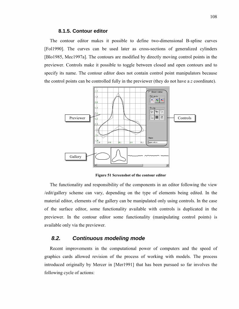
108
8.1.5. Contour editor
The contour editor makes it possible to define two-dimensional B-spline curves
[Fol1990]. The curves can be used later as cross-sections of generalized cylinders
[Blo1985, Mec1997a]. The contours are modified by directly moving control points in the
previewer. Controls make it possible to toggle between closed and open contours and to
specify its name. The contour editor does not contain control point manipulators because
the control points can be controlled fully in the previewer (they do not have a z coordinate).
Gallery
Previewer Controls
Figure 51 Screenshot of the contour editor
The functionality and responsibility of the components in an editor following the view
/edit/gallery scheme can vary, depending on the type of elements being edited. In the
material editor, elements of the gallery can be manipulated only using controls. In the case
of the surface editor, some functionality available with controls is duplicated in the
previewer. In the contour editor some functionality (manipulating control points) is
available only via the previewer.
8.2. Continuous modeling mode
Recent improvements in the computational power of computers and the speed of
graphics cards allowed revision of the process of working with models. The process
introduced originally by Mercer in [Mer1991] that has been pursued so far involves the
following cycle of actions:

109
Editor (L-system, colours, surface, etc.)
Data file
Modeling program
Modifications saved Data re-read
Image generated on the screen
Model regenerated/redrawn
Figure 52 Edit-reread-regenerate scheme used when modeling
In this scheme the user first modifies a component of the model (L-system, colour
specifications etc.), then saves it to a data file and makes the modeling program reread the
modified information. The process is repeated until desired effect is achieved.
Continuous modeling mode frees the user from performing repetitive tasks of issuing
saving and rereading commands, so that he/she can concentrate on the task at hand: editing
of the data. After every change, the modifications are saved automatically and a request is
sent to the modeling program to reread the modified data and redraw and/or regenerate the
model. In this way, updated information transfers continuously from the editor to the
modeling program. Continuous modeling mode has been added to the functionality of L-
studio modeling environment.

110
8.3. Visually controlled parameters
The ability to manipulate parameters controlling the model is almost as important as the
ability to express the model itself. Modification of the model code (L-system) qualitatively
changes the model. On the other hand parameter modification changes quantitative features
of the model. Modification of parameters is a way of performing experiments on the model
by asking �what if?� questions. �What if the branching angle was different (see Figure
53)?� �What if asymmetry was different?� Etc.
Figure 53 Model of Lychnis coronaria (from [Pru1990]) generated for three different branching angles:
10°, 30° and 50°.
In the scope of my research I have improved the methods of controlling parameters by
adding visual programming elements to the design of control panels. These improvements
are discussed in more detail below.
Methods of controlling numerical parameters have been studied in the past [Mer1990,
Mer1991]. Control panels cooperating with parameter editors introduced by Mercer
[Mer1991] made it possible to control numerical and logical parameters visually. Panels
contain controls such as sliders and buttons. Using these controls it is possible to
manipulate parameters contained in text files without actually opening these files in a text
editor.

111
The control panels are designed on a per object basis. In this way, the panels can always
reflect the specific needs of every model or even different aspects of the same model,
depending on the type of experiment or demonstration.
cpfg window
Panels gallery
Panel previewer
Execute/design switch
Figure 54 Model controlled by numerical parameters. The parameters are controlled by a panel.
In the original design [Mer1991] control panels had to be created by manually creating
and editing text files (scripts) that describe the layout and functionality of the controls. The
scripts are interpreted by panel manager. The panel manager is a program that reads the
panel definition and then builds and visualizes the panel. The panel manager is also
responsible for accepting the user input and translating it into the parameter editor�s
actions. The parameter editor is an external program that actually modifies the data file. In
the original implementation, parameter editors were custom-written programs that
internally callsed the ed and awk programs. Finally, the modified parameters are read by
the application program (for example cpfg).

112
Panel definition
file
Panel manager
Parameter editor
Data file
Application
Figure 55 Communication flow involving the panel manager (after [Mer1991])
To simplify the building of control panels, I have researched the possibilities of applying
interactive methods to this process. There are programs and utilities that allow interactive
and visual design of elements of a GUI. Commonly known examples include resource
editors in MS Visual Studio and Qt Designer. These tools make it possible to visually
design elements of a GUI, such as menus or dialog boxes. Control panels are a special type
of dialog box, which contain controls typical to dialog boxes: buttons, sliders, labels, group
frames.
Controls
Layout and alignment
Figure 56 Visual design commands in the panel editor
This kind of tool has been implemented and incorporated into L-studio in a panel editor,
which serves two functions. When in the design mode the panel editor allows the user to
modify a panel:
• Add a control (slider, button, group box, label)
• Delete a control
• Move a control

113
• Arrange a group of controls (modify alignment, distribution)
• Specify and modify the actions associated with a control
In the panel editor the user also specifies the data file, which is controlled by the panel. In
execute mode, the panel editor becomes the panel manager, building and displaying the
controls. It also accepts and handles user input. Because the panel editor follows the
view/edit/gallery design scheme, it is possible to handle more than one panel and perform
the same operations on the set of panels that are performed in other galleries:
• Add new panels,
• Delete existing ones,
• Move panels between objects.
8.4. Visually defined functions
Productions in L+C can contain numerical expressions. The expressions may include
arithmetic operators and function calls. In addition to the standard C++ mathematical
functions and user-defined functions, they may also include graphically defined functions.
Graphically defined functions are used in the following situations:
1) when it is difficult or impractical to find a formula that expresses the desired
function, or
2) when it is necessary to be able to manipulate the values of the function locally.
In the process of modeling, some quantities defining the model cannot be described just
by numbers. For example leaf length is not the same for all leaves even within the same
plant or branch. Instead, it depends on the position of the leaf e.g. its placement on the
stem. This parameter can be thought of as a function: it assigns exactly one value (leaf
length) for every argument from the domain (position on the stem). Similarly, branching
angle is also different for virtually every lateral branch. It can also be described as a
function of position along the stem.

114
It is desirable to have access to this kind of parameters in the form of function calls from
the L-system program, so that they can be used like any other function (trigonometric and
other mathematical functions).
Listing 39 Model of a simple branching structure with lateral branches length and branching angle
controlled by functions. Image generated by the L-system is on the right.
module A(int); module L(float); axiom: SetWidth(0.2) SetColor(2) A(1); derivation length: 22; A(n) : { if (n<=20) { float arg = n/20.0; float brang = 90-90*Fangle(arg); produce F(1) SB Left(brang) F(Flength(arg)) EB SB Right(brang) F(Flength(arg)) EB A(n+1); } else produce F(1) SetColor(3) Circle(0.4); }
The model in Listing 39 refers to two functions Fangle and Flength.
The information that defines these functions can come from different sources.
Sometimes an algebraic formula is available. In that case, functions such as Fangle or
Flength implement the formula and return the result. Sometimes the function can be
defined by experimental data. In that case, the Fangle or Flength functions could calculate
the results by reading the data from an array, an external file etc. However in some cases,
only limited information is available about a function � e.g. the approximate shape of its
plot. This idea can be found for example in [Lin1998, Lin1999]. Both functions (Fangle
and Flength) used in the Listing 39 were defined by drawing the shape of the plot:

115
Flength Fangle
Figure 57 Functions used in the model in Listing 39
Rather than being specified by algebraic formulas, these functions are drawn using the
function editor. The function editor is a b-spline curve editor with additional constrains,
that make sure that the edited curve can be interpreted as a function f(x) = y for any
]1,0[∈x . These constrains are:
• p1.x = 0,
• plast.x = 1,
• pn.x ≤ pn+1.x.
Graphically defined functions can be easily modified by moving control points. For this
reason, graphically defined functions represent extensions of visually controlled
parameters.
Graphically defined functions do not replace functions specified by formulas or other
algorithms that can be easily expressed in a general-purpose programming language such as
C++. Doubtless it is much easier to type a formula such as y = x*x or y = sin(x), rather
than to draw the plot of these functions. Graphically defined functions create a new
category of functional parameters that can be manipulated interactively by the user. The
principal difference between analytic and graphically defined functions is that modifying a
parameter in a formula (a coefficient in a polynomial or exponent in an exponential
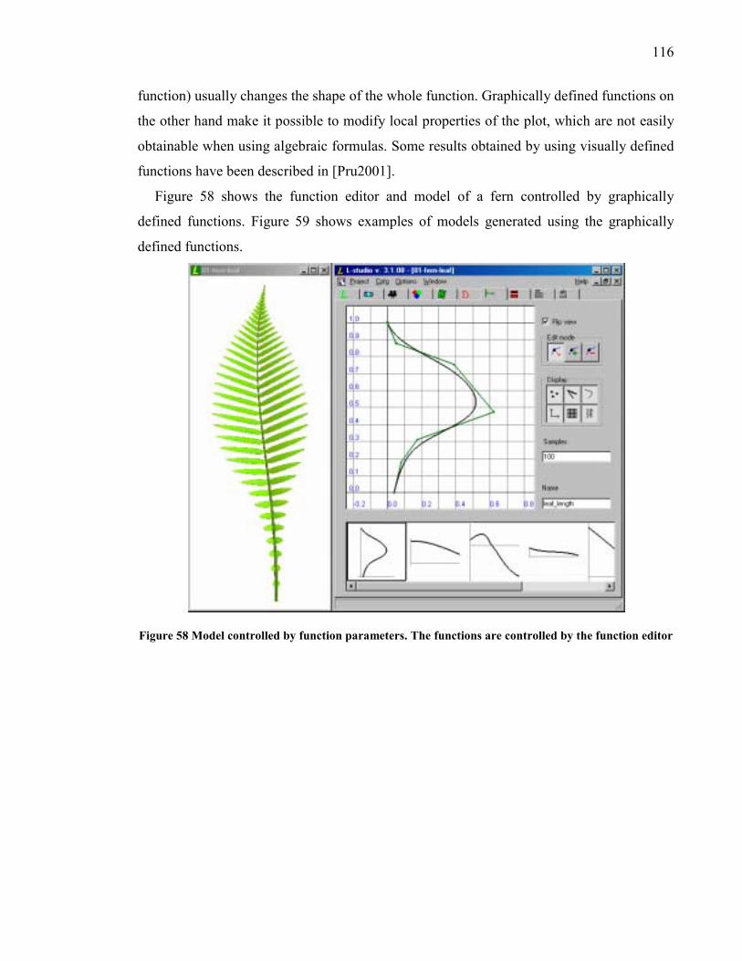
116
function) usually changes the shape of the whole function. Graphically defined functions on
the other hand make it possible to modify local properties of the plot, which are not easily
obtainable when using algebraic formulas. Some results obtained by using visually defined
functions have been described in [Pru2001].
Figure 58 shows the function editor and model of a fern controlled by graphically
defined functions. Figure 59 shows examples of models generated using the graphically
defined functions.
Figure 58 Model controlled by function parameters. The functions are controlled by the function editor

117
Figure 59 Models of Pellaea falcata and Indian paintbrush created using graphically defined functions
(from [Pru2001])
8.5. Visual interaction with the model
The need for direct interaction with the model was recognized some time ago. Power et
al. presented some research on visual manipulation of models generated using L-systems in
[Pow1999]. In this paper the authors give an overview of their application ilsa (interactive
L-string arranger) that allows a user to interactively manipulate the geometry of a plant
model. The design of the ilsa is based on the flow of control presented in Figure 60.
String saved String read
axiom
L-string File L-string
L-string File String saved String read
derivation User�s manipulation
ilsa cpfg
Figure 60 Information flow between cpfg and ilsa

118
To manipulate a plant model using cpfg/ilsa, the user first needs to create a model in
cpfg. Once the model is generated the L-string is saved to a disk file. The file is then read
by ilsa. Ilsa provides a display window where the user can interactively manipulate organs:
turn, rotate and bend. Ilsa inserts corresponding turtle commands in the L-string to reflect
the modifications. Then the string can be saved in a disk file and read back into cpfg. Work
by Power provides a method for interactive manipulation of the geometry of generated
structures.
I propose another method of interaction with models. My more general method is based
on the ability to modify the string interactively by inserting a predefined module. The user
can point to an element of the model on the screen and request to insert a predefined
module (X) in the string. The module X is inserted in the string right before the module
pointed to by the user. Figure 61 shows a visualization of the following L-system:
Listing 40 L-system implementing simple interactive pruning
Axiom: F1[+F2][-F3] X ! ;F4(0.2)%
Click here
F2 F3
F1
F4 F2
F1
Figure 61 Module X inserted interactively
Initially the structure consists of three segments F1, F2 and F3. When the user selects the
branch corresponding to the module F3 the string is modified:
F1[+F2][-XF3]
During the next derivation step, the production p1 is applied and the module X is replaced
with the segment F4, which is shorter and drawn using a different colour. The remainder of

119
the branch (module F3) is removed by the module % (cut). In this way the user interactively
modified the development of the model. This method can also be used to induce more
complex actions than cutting a branch. For example, module X can be a signal that induces
flowering in a selected branch. A short discussion on further applications is presented in
9.1.2.

120
9. Conclusions
9.1. Summary of contributions
The research described in this dissertation contributes to three areas in the domain of
plant modeling:
a) L-systems as a mathematical formalism,
b) L-systems as a programming language,
c) Visual and interactive modeling.
The contributions belonging to the first two categories have been summarized and
implemented in a new L-systems based modeling language L+C, which I have defined and
implemented. Evaluation of the language from the conceptual and practical points of view
is presented in section 9.1.1. Summary of my contributions in the domain of visual and
interactive modeling are presented in section 9.1.2.
I have also created a plant modeling environment, L-studio. The environment is
comprised of three principal elements: L-system based modeling programs (cpfg and lpfg)
and a set of tools integrated into the program called L-studio. Cpfg is an L-system based
plant modeling program. It was originally created by Prusinkiewicz. Further extensions
were added by James, Hammel, Hanan, Měch and myself [Han1992, Mec1997a,
Mec1998]. I have designed and implemented lpfg. Lpfg is an L-system based modeling
program which implements and uses the L+C modeling language. The language is
described in chapter 3.4. The user�s manual for lpfg is presented in appendix A.
9.1.1. Evaluation of L+C
Users of L-systems have identified shortcomings of L-systems as a formalism and a
modeling language. These shortcomings are described in chapter 3 together with proposed
solutions. The number and significance of required modifications and extensions justified
creation of a new language instead of extending the existing syntax. As a result I designed a
new L-system-based modeling language L+C. It has been designed from scratch with a

121
well-defined set of requirements. This approach made it possible to include new elements
in a cleanly and consistently.
The main conceptual contributions to the formalism of L-systems are fast information
transfer and the new-context construct. Fast information transfer is an alternative method of
propagating information and signals in models of both linear and branching structures. It
has tow advantages over the traditional method of information transfer using context-
sensitive productions:
a) It allows a clearer structure for models than in traditional L-systems, which need
many derivation steps to propagate a signal.
b) The signal can be propagated throughout the entire structure in one derivation step.
The time required is proportional to the number of modules in the string so the
method is O(N) as opposed to O(N2) when using context-sensitive methods.
New context facilitates implementation of fast information transfer in models without
the use of a global variable (in the case of linear structures) or a stack (in the case of
branching structures). Expressing fast information transfer using only local data (a
modules� parameters and variables local to the productions) is consistent with the spirit of
L-systems � expressing models in the local terms.
The introduction of user-defined types increased the expressive power of L-systems as a
modeling language and allowed creation of models in which the modules are associated
with many parameters. A large number of parameters associated with modules are required
in (among others) genetic and biomechanical models.
An important decision in the design of L+C was to base its syntax on an existing
general-purpose language, C++. L+C adds L-system-specific constructs to C++ while
preserving all the expressive power of C++. The flow of control is governed by the
declarative nature of L-systems rather than by the imperative paradigm as in C++.
This decision had two further effects:
a) The syntax of elements typical to C++ (e.g. declarations of structures, functions
etc.) are the same as in C++. This diminishes the learning for new users of the
language, if they are already familiar with C++.
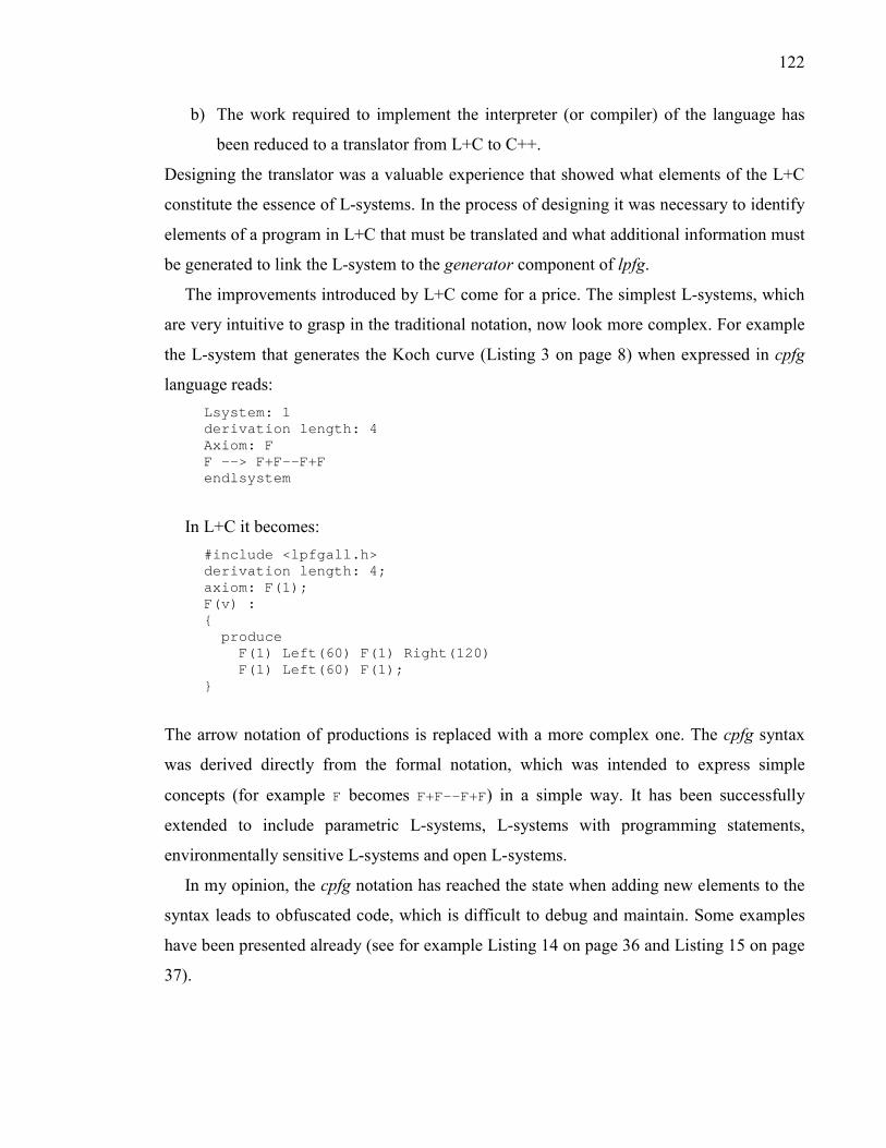
122
b) The work required to implement the interpreter (or compiler) of the language has
been reduced to a translator from L+C to C++.
Designing the translator was a valuable experience that showed what elements of the L+C
constitute the essence of L-systems. In the process of designing it was necessary to identify
elements of a program in L+C that must be translated and what additional information must
be generated to link the L-system to the generator component of lpfg.
The improvements introduced by L+C come for a price. The simplest L-systems, which
are very intuitive to grasp in the traditional notation, now look more complex. For example
the L-system that generates the Koch curve (Listing 3 on page 8) when expressed in cpfg
language reads: Lsystem: 1 derivation length: 4 Axiom: F F --> F+F--F+F endlsystem
In L+C it becomes: #include <lpfgall.h> derivation length: 4; axiom: F(1); F(v) : { produce F(1) Left(60) F(1) Right(120) F(1) Left(60) F(1); }
The arrow notation of productions is replaced with a more complex one. The cpfg syntax
was derived directly from the formal notation, which was intended to express simple
concepts (for example F becomes F+F--F+F) in a simple way. It has been successfully
extended to include parametric L-systems, L-systems with programming statements,
environmentally sensitive L-systems and open L-systems.
In my opinion, the cpfg notation has reached the state when adding new elements to the
syntax leads to obfuscated code, which is difficult to debug and maintain. Some examples
have been presented already (see for example Listing 14 on page 36 and Listing 15 on page
37).

123
Also the decision to use single ASCII symbols or pair of symbols as identifiers of turtle
commands in cpfg leads to expressions such as this one11:
Listing 41 Example of a complex successor written in cpfg
@OF(l)[,@v&(90)f(ran(0.01))^(90)@c(0.5*2)]
Because cpfg is not a free-form language, the possibilities of formatting productions are
limited. I claim that the equivalent of code rewritten in L+C (see Listing 42), although
longer, is more legible:
Listing 42 Equivalent of code from Listing 41 rewritten in L+C
Sphere0 F(1) SB DecColor RotToVert Down(90) f(ran(0.01)) Up(90) Circle(0.5*2) EB;
Better legibility is particularly evident in more complex models. Because L+C was
designed to make it possible to write more complex models, it can be assumed that this goal
has been achieved.
9.1.2. Visual and interactive aspects of modeling
I have also researched improvements in the domain of visual modeling. The concept of
visually controlled parameters has been extended to include graphically defined functions.
Corresponding visual tools to manipulate these functions have also been constructed and
implemented. Graphically defined functions are one of the fundamental elements of inverse
modeling [Pru2001]. The ability to manipulate the shape of the function�s plot makes it is
easy to experiment with models, for example by locally modifying the controlling
functions.
The concept of continuous modeling leads to results that proved to be useful both in the
course of modeling work and in the case of presentations and live demonstrations.
I have also implemented a new method of direct interaction with models. The result is
the concept of modules that are interactively inserted into the model. Modules inserted
11 An actual successor from a model of Terminalia catappa [Mec1996].
124
interactively do not break the link between the algorithm that generated the model, internal
representation of the model and its graphical representation. The model can handle the
modules inserted by the user and react on them.
Possible applications of interactively inserted modules include modeling of:
a) pruning,
b) grafting,
c) local mutations,
d) presence of pests,
e) application of pesticides.
9.2. Future work
In this section I briefly describe problems and questions that have been identified during
my research but have not been addressed. These problems may constitute the foundation for
future work on the modeling using L-systems and further development of L+C.
9.2.1. Missing elements
L+C does not include sub-L-systems. Sub-L-systems introduced by Hanan [Han1992]
make it possible to create hierarchical models. Adding this concept to L+C is still an open
problem because of differences of how local variables are handled in sub-L-systems and in
C++.
Developmental surfaces [Mec1997a] are also not available in L+C. The problem of how
to model growing surfaces such as leaves and petals is a very general and interesting
challenge that definitely deserves work.
9.2.2. Problems worth revisiting
Object-oriented elements in L+C
One of the most interesting concepts that warrants further research of the L+C modeling
language is the incorporation of concepts from object-oriented programming. In particular
these concepts include:
a) inheritance.
b) Polymorphism.

125
c) Data hiding,
Inheritance
The concept of inheritance makes it possible to conceptually organize the elements of a
model into a hierarchical structure. Elements that are lower in the structure inherit (share)
features of the elements higher up. For example age can be considered a characteristic
shared by all organs in a plant. It is therefore appropriate to define it at the top level of the
hierarchy as a characteristic for all modules to share. Other examples that may characterize
entire classes of modules, and therefore could be inherited (shared) include: amount of
photosynthates produced by leaves, length and diameter of internodes, diameter of fruits.
In each case inheritance could be used to define modules that represent specific organs
by adding new properties to the base modules.12
Polymorphism
In object-oriented languages polymorphism makes it possible to state that some
calculations are to be performed, without giving details that may depend on the object type.
Polymorphism is achieved using virtual methods (or functions), which have the same name
but different meaning depending on the object type. For example, in the context of plant
modeling, an important quantity is the amount of resources, such as carbon, allocated to
specific modules. All organs use carbon for growth and maintenance, but functions that
describe the amounts are different for different organs (for example, leaf vs. fruit). Thus the
allocation of carbon may be defined using a virtual method at the level of organs and then
specialized for individual organ types.
Data hiding
When dealing with data structures, manipulation can be performed using one of two
approaches. The first approach is to access all members of the data structure directly. The
values can be read and modified at will. The second approach is to encapsulate all
operations that can be performed on the data structure into a set of functions. In the
programming practice it has been found that this second approach works better. This is
especially true when the members of a data structure are interdependent. The specialized
functions guarantee that these interdependencies are always satisfied and the information
12 A different concept of inheritance in L-systems has been proposed by Borovikov in [Bor1995]
126
represented by the structure is internally consistent. At present, the L+C language makes it
possible to associate methods with data structures, but does not make it possible to
associate methods with module types. Consequently, the concept of data hiding is not fully
supported at the level of modules.
What are further consequences of deriving the string forward and backward?
More consideration can be given to the problems related to sequential derivation of the
string and explicit control over the direction of the process. Fast information transfer relies
on the ability to control the derivation direction. Also the % (cut) module introduced by
Hanan [Han1992] requires the derivation to be performed from left to right. When the
derivation is performed in the opposite direction branch cutting cannot be performed by
skipping to the end of the current branch. What are other effects of sequential derivation
forward or backward, and how the sequential execution of derivation steps alters the
properties of L-systems? What is the relationship between fast information transfer and
attribute grammars? More theoretical research would help answer these questions.
Dynamic data structures as modules� parameters
Currently it is clear how to use simple (C++ built-in) or compound types (structures) as
modules� parameters. What is not clear is how to use non-trivial dynamic data structures
(linked-lists, stacks etc.) as a modules� parameters. The main problem arises because the
elements of these structures are allocated dynamically and require special handling when
being deleted, copied etc. Various methods of resource transfer and resource management
should be tested. In particular some consideration should be given to the use of STL-
defined containers as a modules� parameters.
It is worth noting that the problems described above are a direct consequence of using
C++ as the foundation of L+C. For example, these problems are not present in L-Lisp
created by Erstad [Ers2002]. L-Lisp is an L-systems framework written in Common Lisp, a
language with garbage collection mechanism.
127
Query modules vs. new context
Query modules contain meaningful information after the �interpretation step for the
environment� has been performed. This step is performed after string rewriting is
completed. In particular, query modules do not contain any meaningful information
immediately after they are created (e.g. when they are in the new context). It would be
interesting to consider the changes in the L+C language semantics to disallow query
modules in the new context, or alternatively perform the interpretation while deriving. This
could be applied only when deriving forward.
Module names
The L+C specifies that a module name must be a valid C++ identifier. This restriction
disallows module names such as [ and ]. These identifiers have a well established position
in L-systems notation and it is tempting to consider the possibility of allowing them as
module identifiers.
However lifting the restriction on module names would imply a major redesign of the
way the L+C to C++ translator works. Currently L2C works under the assumption that a
single token is enough to recognize L+C constructs. But [ and ] symbols can appear in C++
code when they have different meaning (array element operator). Consequently allowing [
and ] as valid module identifiers would probably require full syntax analysis of the L+C
source code.
9.3. Closing remarks
The main goal of my research was to improve the process of plant modeling. The L+C
modeling language, implemented in lpfg, and the modeling environment L-studio are a
practical realisation of the concepts I have introduced or extended in the scope of my
research. The modeling system is distributed by the University of Calgary and is currently
used in approximately 100 locations worldwide. L+C�s applications are not limited to the
plant modeling but also include applications in the domain of subdivision curves [Pru2002].
128
Appendices
A. LPFG user’s guide lpfg is a plant modeling program. The models are expressed using a formalism based on
L-systems. The formalism, called the L+C modeling language adds L-systems specific
constructs to the C++ programming language.
A.1. Hardware requirements
lpfg does not have any specific hardware requirements. It uses OpenGL to generate
images it is therefore strongly recommended to use graphics cards capable of displaying
graphics with resolution at least 1024x768 pixels at 24 or 32 bit depth. A mouse or an
equivalent pointing device is also required.
A.2. Software requirements
lpfg runs under MS Windows operating systems (9x/Me/NT v. 4.0/2000). It requires a
C++ compiler capable of generating Windows DLL�s (Dynamic Link Libraries). lpfg was
originally developed and tested using MS Visual C++ compiler v. 6.0.
A.3. Installation
lpfg is distributed together with L-studio. Refer to the L-studio installation guide on how
to install it.
A.4. Command line options
lpfg is designed as an element of a modeling environment, such as L-studio or Vlab.
Usually it will be invoked by the environment rather than directly by the user. This sections
presents the command line switches supported by lpfg. lpfg [-a] [-d] [-b] [-wnb] [-wnm] [-wr w h] [-wpr x y] [-wp x y] [-w w
h] [–out filename] [colormap_file.map] [material_file.mat]
[animation_file.a] [functionset_file.fset] [drawparameters_file.dr]
[viewparameters_file.v] [contourset_file.cset] [environmentfile.e]
Lsystemfile.l
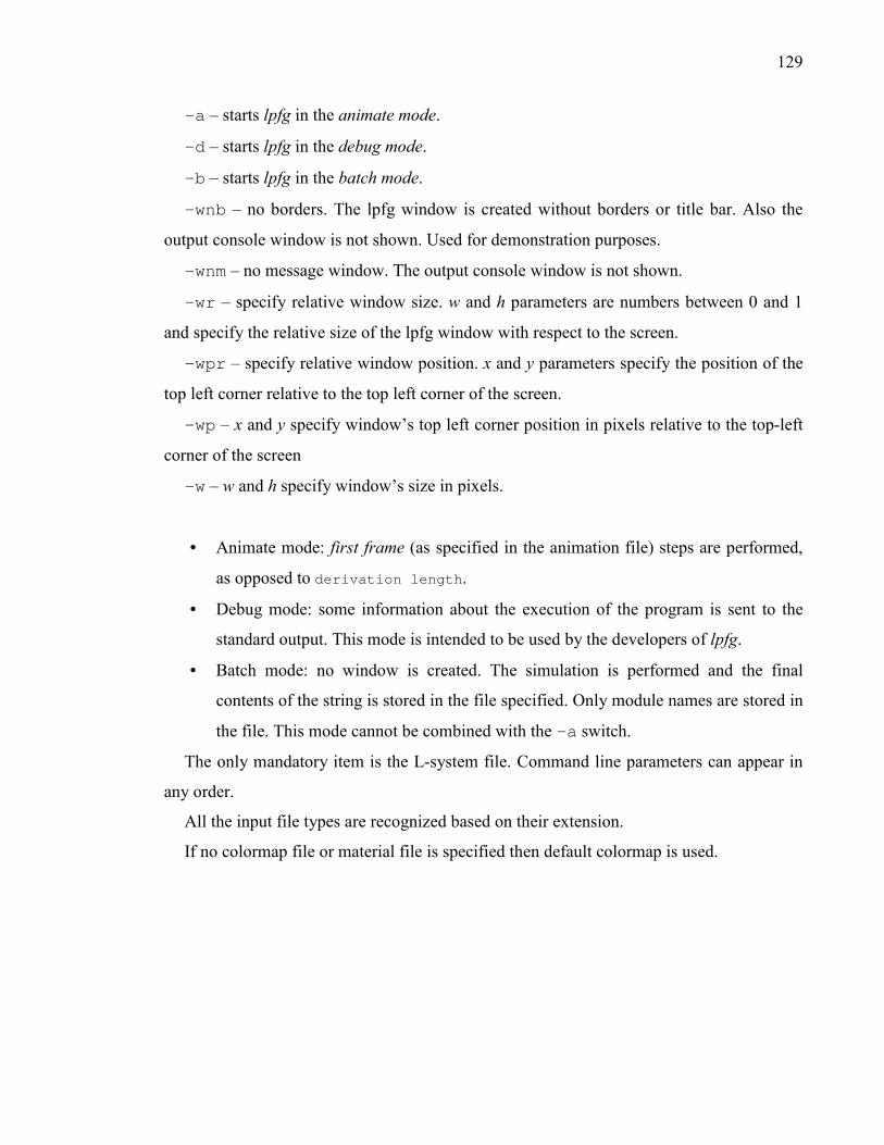
129
-a � starts lpfg in the animate mode.
-d � starts lpfg in the debug mode.
-b � starts lpfg in the batch mode.
-wnb � no borders. The lpfg window is created without borders or title bar. Also the
output console window is not shown. Used for demonstration purposes.
-wnm � no message window. The output console window is not shown.
-wr � specify relative window size. w and h parameters are numbers between 0 and 1
and specify the relative size of the lpfg window with respect to the screen.
-wpr � specify relative window position. x and y parameters specify the position of the
top left corner relative to the top left corner of the screen.
-wp � x and y specify window�s top left corner position in pixels relative to the top-left
corner of the screen
-w � w and h specify window�s size in pixels.
• Animate mode: first frame (as specified in the animation file) steps are performed,
as opposed to derivation length.
• Debug mode: some information about the execution of the program is sent to the
standard output. This mode is intended to be used by the developers of lpfg.
• Batch mode: no window is created. The simulation is performed and the final
contents of the string is stored in the file specified. Only module names are stored in
the file. This mode cannot be combined with the –a switch.
The only mandatory item is the L-system file. Command line parameters can appear in
any order.
All the input file types are recognized based on their extension.
If no colormap file or material file is specified then default colormap is used.

130
A.5. User interface
A.5.1. View manipulation
• Rotation � lpfg uses XY rotation interface based on the continuous XY rotation as
described by Chen et al. in [ref]. The model is rotated around the Y axis when the
mouse is moved horizontally and around X axis when the mouse is moved
vertically. To start rotating press left mouse button.
• Roll � to roll the model around the Z axis press Shift + middle mouse button.
Moving the mouse to the right rotates the model clockwise, moving the mouse to
the left rotates the model counter-clockwise.
• Zoom � to start press Ctrl + left mouse button or the middle mouse button. Moving
mouse up zooms in, moving down zooms out.
• Pan � to start press Shift + left mouse button.
• Change frustum angle � to start press Ctrl + middle mouse button. Moving mouse
up increases the angle, moving down decreases the angle. This operation has effect
only in the perspective projection mode.
A.5.2. Menu commands
To display menu click the right mouse button inside the lpfg window.
Figure 62 Lpfg menu

131
Step Advances simulation to the next step. This may correspond to
more than one derivation step if parameter step in the animate
file is present and specifies a value greater than 1.
Run Starts or resumes the animation.
Forever Starts or resumes the animation. After the last frame is reached
the animation returns to the first frame and continues.
Stop Stops the animation.
Rewind Resets the animation to the first frame.
Don�t animate Stops the animation and generates the image in the still mode
(performs the number of derivation steps as specified in the
derivation length statement).
Restore view Resets rotation, zoom, pan, frustum and roll to the default
values.
Reset !!!! Rotation Resets rotation.
Reset !!!! Zoom Resets zoom.
Reset !!!! Pan Resets pan.
Reset !!!! Roll Resets roll.
Reset !!!! Frustum Resets frustum (not implemented yet).
Show axis Turns on or off display of coordinate system axis in the left
lower corner.
Output !!!! BMP Creates image file filename.bmp containing the current state
of the window. Filename is the name of the L-system file.
Output !!!! Rayshade Creates a rayshade file (not implemented yet).
Output !!!! POV-Ray Creates a POV-ray file (not implemented yet).
Output !!!! Postscript Creates a postscript file filename.ps. Filename is the name of
the L-system file. All modules F are drawn as lines, even if
line style is set to cylinder. If line style is polygon
then modules F are drawn as lines of properly scaled width. The
only other module supported is Circle and Circle0. No other
modules are visualized.

132
A.6. L-system file
A typical L-system program file has the following format:
Listing 43 A typical L-system in L+C
#include <lpfgall.h> derivation length: d; // declarations of data structures // declarations of functions // module declarations ignore: module list; axiom: parametric word; lcontext < predecessor > rcontext : { … produce parametric word; }
All elements of a program can appear in any order except for the following restrictions:
1) all elements referred to in a statement must be declared beforehand. For example: types
used as parameters of a module must be declared before the module can be declared.
Also modules that appear in the ignore or consider statement must be declared before.
2) Productions are matched in the order in which they are declared.
A.6.1. Mandatory elements
The mandatory elements in every L-system are the statements: derivation length and
axiom.
A.6.2. Include files
The first line in the L-system is the include statement. The lpfgall.h include file
includes the following standard header files:
133
• memory.h and stdlib.h � standard C header files. Required by the code generated
by the L2C translator
• lparams.h � this file contains the declarations and definitions that are used by lpfg,
L2C translator and the C++ code generated by the L2C translator. For example:
maximum number of parameters per module, maximum number of modules in a
production predecessor etc.
• lintrfc.h � this file contains declarations and definitions that are used by lpfg and
the C++ code generated by the L2C translator. For example: types used for
communication between the L-system and lpfg, predefined vector types (see section
Predefined functions and structures)
• lsys.h � this file contains declarations and definitions required by the C++ code
generated by the L2C translator. These include definitions of some predefined
functions: Forward(), Backward(), etc.
• stdmods.h � this file contains declarations of predefined modules.
lpfg standard header files should be treated the same way as the standard C header files:
they should never be changed or edited in any way. If they are models might not compile,
stop working or lpfg may hang or crash.
In addition to the required include files any other include files can be also specified.
A.6.3. derivation length:
The derivation length statement has the following form: derivation length: integer expression ;
The integer expression is any arithmetic expression that has value of type integer or a
value that can be converted into an integer. The expression can be a function call (or it can
contain a function call). The value of this expression is evaluated once when the model is
generated in the still mode, but may be evaluated more than once in the animate mode. It is
the user�s responsibility to make sure that the expression has always the same value. For
example, in the statement
derivation length: ++i;

134
the expression ++i will return different value every time it is evaluated. In the animate
mode this may result in an infinite number of steps.
A.6.4. Declarations of data structures and functions
Syntax of declarations of data structures and functions are the same as in C++.
A.6.5. Module declaration
Every module must be declared before it can be used in the axiom or in a production.
The module declaration has the following form:
module Identifier(parameters listopt); or
module Identifier;
The parameters list is a comma separated list of types. These are sample module
declarations:
module A(int, float); module B(); module C(data, float); module D;
Module A is declared to have two parameters: one of type int and another one of type
float. Module B is declared to have no parameters. Module C is declared to have two
parameters of type data and float where data is a previously defined type (for example a
structure). Module D is declared to have no parameters and uses the shortcut notation
(without empty parentheses).
Note: All types must be declared before they can be used as parameters in module�s
declaration. In particular this applies to all user-defined types (structures).
Note: Parameters of modules (unlike parameters of functions) don�t have names.
Consequently it is illegal two give them names. For example: module A(int id, float length);

135
will cause the L2C translator to signal an error. But it is legal and often useful to
comment on module parameters: module A(int /* id */, float /*length*/);
Note: Parameter type must be a single identifier. For example the following are valid
C++ type specifiers but cannot be used as parameter types of modules: unsigned int
char*
If a type of this kind is needed it is necessary to use typedef to create an identifier for
that type. For example: typedef unsigned int uint;
typedef char* text;
It is possible to declare a module and specify the module�s numerical identifier in its
declaration. The syntax for this declaration is:
module Identifier(parameters listopt) = constant expression; or module Identifier = constant expression;
This syntax should not be used in the user�s L-systems and is reserved for the include
file that declares standard modules (stdmods.h).
A.6.6. Axiom
The axiom statement has the following form: axiom: parametric word ;
The parametric word is a sequence of modules. Initial value for every modules�
parameters must be specified. Initial value of a parameter must be an expression of the
same type as the type of the parameter. All conversion rules from C++ apply. In the
following code:
module A(int, float);

136
axiom: A(5, 2.7-sin(M_PI/3)) A(1-abs(v), 5);
the axiom contains two modules of type A. Modules A have two parameters: an int and a
float. The first module A will have its first parameter initialized with number 5. The
second parameter will be initialized with the value of expression 2.7-sin(M_PI/3) where
sin is a previously declared function (in math.h in standard C++)
The second module A will have its first parameter initialized with value 1-abs(v) where
abs is a previously defined function (in stdlib.h in standard C++) and v is a variable
previously defined. The second parameter will be initialized with a value of 5 (an integer)
implicitly converted into a float 5.0f.
If a module has no parameters its name can be followed by empty parentheses or the
parentheses can be omitted altogether:
module B(); axiom: B() B;
In this example axiom contains two modules B. B has no parameters.
A.6.7. ignore, consider statements
ignore statement has the following form: ignore: list of modules ;
The list of modules contains modules identifiers separated by blank characters (spaces,
tabs or new lines). The list is terminated with a semicolon. For example: ignore: A F P;
Syntax for the consider statement is analogous: consider: list of modules ;
ignore and consider statements are mutually exclusive. By default all modules are
considered when matching contexts. The ignore statement specifies the modules that
should be ignored when matching contexts. The consider statement specifies the list of
modules that should be considered when matching contexts. If consider statement is used
then only the modules listed in the consider statement are considered. For detailed
information on matching productions see section How the productions are matched.

137
Note: SB and EB modules are always considered. Listing them in the consider
statement is unnecessary. Listing them in the ignore statement is allowed but has no
effect.
A.6.8. Start, End, StartEach and EndEach control statements
The syntax for these statements is: Start | End | StartEach | EndEach :
{
…
}
These statements should be treated as procedures. Any legal C++ statements are allowed
inside their body. User can also specify here the direction of the derivation process (see
predefined functions).
Start is always executed before axiom.
StartEach is executed before every derivation step. EndEach is executed after every
derivation step.
End is executed after the last derivation step only when the program is not in the
animate mode. This means:
• after the program has been started without the –a switch
• when the user selects Don�t animate from the menu
A.6.9. Productions
There are three main types of productions:
a) context-free productions
b) context-sensitive productions
c) new-context-sensitive productions
Context-free productions have the following form: strict predecessor :
{
…

138
}
Context-sensitive productions have the form lcontextopt < strict predecessor > rcontextopt:
{
…
}
At least one of contexts must be specified.
New-context sensitive productions have one of the following forms: flcontext << strict predecessor > rcontextopt :
{
…
}
lcontextopt < strict predecessor >> frcontextopt :
{
…
}
Every component of the predecessor (contexts and the strict predecessor) consists of one
or more modules. Modules in the predecessor must include names of their formal
parameters. Formal modules are separated by commas. If a module has no parameters its
name must be followed by a pair of parentheses ().
For example:
A(nl, fl) < B() > A(nr, fr) C(d, v) : { … }
specifies a production that has one module B as its strict predecessor. Module A is the left
context and modules A and C are the right context. Names of the formal parameters must be
unique within a predecessor. This is why parameters in the left context have postfix l.
Production can contain any valid C++ code. Productions also usually contain one or more
produce statements.

139
A.6.10. produce statement
Produce statement specifies production�s successor. It is allowed only inside
productions. It has the following form: produce parametric-wordopt;
Parametric-word has the same syntax as in axiom. If it is omitted then the successor of
the production is empty. Effectively it removes the modules present in the strict predecessor
from the derived string.
Examples: produce A(4, 5.2) B A(1, 0.5); produce ;
If a production does not execute a produce statement then lpfg will continue searching
for other productions matching the current position in the string. If no production is found
then default (identity) production is applied.
A.6.11. Decomposition rules
Decomposition rules make it possible to decompose a module in the string into several
components. After axiom and every derivation step a decomposition step is performed.
Decomposition is performed as long as the string does not contain any modules that can be
further decomposed or the maximum decomposition depth is reached. Syntactically
decomposition rules are very similar to regular productions except for the following
differences:
• only one module in the strict predecessor is allowed,
• decomposition rules are always context-free.
When the statement decomposition: is present in the L-system it specifies that all the
following rules are decomposition rules until the end of the source file or until
production: or interpretation: statement is encountered. To specify maximum
decomposition depth the maximum depth: statement is used. It must be placed in the global
scope after the decomposition:. The syntax of the maximum depth statement is as
follows: maximum depth: integer-expression ;
140
The default maximum decomposition depth is 1.
Note: L-system can contain many decomposition sections but only one maximum
depth: statement is allowed for decomposition. The same applies to the interpretation
rules.
Decomposition rules can be recursive, e.g. the module in the strict predecessor can
appear in the successor. For example:
#include <lpfgall.h> module A(int); axiom: A(5); derivation length: 0; decomposition: maximum depth: 6; A(n) : { if (n>0) produce F(1) A(n-1); }
The L-system above will generate five modules F(1).
Note: decomposition is internally implemented by a recursive call to a function. If the
maximum depth is a very large number the thread stack might overflow causing lpfg to
crash.
A.6.12. Interpretation rules
Interpretation rules are syntactically very similar to the decomposition rules. To specify
interpretation rules the interpretation: statement must be specified. Like the
decomposition rules interpretation rules must have exactly one module in the strict
predecessor and must be context-free. At most one maximum depth: statement is allowed
per L-system.

141
Interpretation rules are executed only during the interpretation of the string. Modules
produced by interpretation rules are not inserted into the string but are just used as
commands for the turtle during the interpretation steps.
The interpretation step is performed in the following cases:
1. When redrawing the model in the window
2. When generating output file (rayshade, POVray, postscript)
3. When calculating the view volume.
4. After axiom and each derivation step if any of the productions contains query or
communication modules
Note: interpretation and decomposition rules can be very helpful in properly
expressing models. They can be used to separate the functional aspect of the model from
its visual aspect. But these rules can be also misused. In particular interpretation rules
might add time overhead. It is a matter of experience and good design intuition to use
them wisely and effectively.
Note: in lpfg it is possible to specify regular productions after decomposition and
interpretation rules. To specify regular productions use the production: statement. This
possibility leads to another methodology of writing models. Instead of dividing the model
into production, decomposition and interpretation sections all rules that apply to one type
of module can be grouped together. For example:
production: A() : { … } decomposition: A() : { … } interpretation: A() : { … } production: B() > A() : { … } decomposition: B() : { … }
Etc.

142
A.6.13. Predefined functions and structures
Here is the summary of the predefined functions and structures provided by lpfg:
void Forward()
This function specifies that the derivation of the string should be performed forward �
from left to right. This is default. void Backward()
This function specified that the derivation of the string should be performed backward �
from right to left.
Forward and Backward can be used anywhere in the code where it is legal to call a
function. They take effect the next time derivation is performed. In particular if called in
the StartEach statement they affect the current derivation step.
void Printf(const char*, …).
This function is similar to the standard C function printf. Its use is recommended over
the printf for the following reasons:
• Output generated by printf is not stored in the lpfg.log file.
• In the future releases lpfg might be not connected to any console but instead provide
its own output window (like cpfg�s message log). In that case output of printf
would not be visible anywhere.
float ran(float range)
Generates a pseudorandom number uniformly distributed in the range [0, range).
float func(int id, float x)
This function returns the value of the function specified in the function-set file (if one is
present in the command line). First parameter specifies the ordinal number of the function
as in the .fset file. It must be in the range [1, num of functions]. The second is the x value
for which the y value is requested. Parameter x must be in the range [0, 1].
143
If the parameter id is incorrect (outside the range) value 0 is returned and warning
message is printed. If the parameter x has invalid value then:
• if x<0 then func(id, 0) is returned
• if x>1 then func(id, 1) is returned
In addition lpfg provides four structures that represent vectors. The structures are:
struct V2f { float x, y; }; struct V3f { float x, y, z; }; struct V2d { double x, y; }; struct V3d { double x, y, z; };
These structures are used as parameters for some predefined modules. They can also be
used in the user�s code in the L-system. Additionally if the preprocessor�s symbol
NOAUTOOVERLOAD is not defined before #include <lpfgall.h> these structures receive
additional functionality: operators for addition of two structures of the same type and
multiplying a vector by a number. For example: V2f a(1.5, 2.0), b(0, 0.5); V2f c = a + 2.5*b;
Refer to the file lintrfc.h in the lpfg/include directory to see full definition of these
structures.
A.6.14. Predefined modules
The following table lists all the predefined modules.

144
Module Description Equivalent
in cpfg
Modeling branching structures SB() Starts a new branch by pushing the current state of the turtle
on the turtle stack.
[
EB() Ends a branch by popping the state of the turtle from the
turtle stack.
]
Cut() Cuts the remainder of the current branch. When detected in
the string during the generation process, the module and all
following modules up to the closest unmatched EB module
are ignored for derivation purposes. If no unmatched EB
module can be found, symbols are ignored until the end of the
string.
%
Changing position and drawing Turtle commands
F(float /*d*/) Moves forward a step of length d and draws a line segment
from the original position to the new position of the turtle.
F(d)
f(float /*d*/) Moves forward a step of length d. No line is drawn. f(d)
MoveTo (float /*x*/, float /*y*/, float /*z*)
Sets the turtle position to x, y, z. @M(x,y,z)
MoveTo2f (V2f /*p*/)
Moves the turtle to point p. z coordinate is assumed to be 0. @M
MoveTo2d (V2d /*p*/)
Same as MoveTo2f @M
MoveTo3f (V3f /*p*/)
Same as MoveTo2f except that the z coordinate is specified
by the parameter p.
@M
MoveTo3d (V3d /*p*/)
Same as MoveTo3f @M
Affine geometry support
Line2f (V2f /*p1*/, V2f /*p2*/)
Draws a line from the point specified by p1 to the point p2. z
coordinates are assumed to be 0. After the interpretation of
the module the turtle position is equal to p2. Heading, left

145
and up vectors are not changed. If the distance between p1
and p2 is less than ε13 the module is ignored.
Line2d (V2d /*p1*/, V2d /*p2*/)
Same as Line2f
Line3f (V3f /*p1*/, V3f /*p2*/)
Same as Line2f, except that z coordinates are specified in
the p1 and p2 parameters
Line3d (V3d /*p1*/, V3d /*p2*/)
Same as Line3f
LineTo2f (V2f /*p*/)
Draws a line from the current turtle position to the point p. z
coordinate is assumed to be 0. After the interpretation of the
module the turtle position is equal to p. Heading, left and up
vectors are not changed. If the distance from the current
position to p is less than ε the module is ignored.
LineTo2d (V2d /*p*/)
Same as LineTo2f
LineTo3f (V3f /*p*/)
Same as LineTo2f, except that z coordinate is specified by
the parameter p.
LineTo3d (V3d /*p*/)
Same as LineTo3f
LineRel2f (V2f /*p*/)
Draws a line from the current turtle position to the point
p2 = (turtle position) + p. z coordinate is assumed to be 0.
After the interpretation of the module the turtle position is
equal to p2. Heading, left and up vectors are not changed. If
the length of vector p is less than ε the module is ignored.
LineRel2d (V2d /*p*/)
Same as LineRel2f
LineRel3f (V3f /*p*/)
Same as LineRel2f, except that z coordinate is specified
by the parameter p.
LineRel3d (V3d /*p*/)
Same as LineRel3f
Turtle rotations Left (float /*a*/)
Turns left by angle a around the U axis +(a)
Right (float /*a*/)
Turns right by angle a around the U axis -(a)
Up(float /*a*/) Pitches up by angle a around the L axis ^(a)
13 ε is defined as 0.00001

146
Down (float /*a*/)
Pitches down by angle a around the L axis &(a)
RollL (float /*a*/)
Rolls left by angle a around the H axis \(a)
RollR (float /*a*/)
Rolls right by angle a around the H axis /(a)
TurnAround() Turns around 180 degrees around the U axis. This is
equivalent to Left(180) or Right(180). It does not roll
or pitch the turtle
|
SetHead (float /*hx*/, float /*hy*/, float /*xz*, float /*ux*/, float /*uy*/, float /*uz*)
Sets the heading vector of the turtle to hx, hy, hz and the up
vector to ux, uy, uz. The values do not need to specify
normalized vectors. The module is ignored if any of the
following is true:
a) hx,hy,hz specify a vector of length less than ε
b) ux,uy,uz specify a vector of length less than ε
c) Length of the cross product of new H and U is less than ε
@R
(hx,hy,hz,
ux,uy,uz)
RollToVert() Rolls the turtle around the H axis so that H and U line in a
common vertical plane with U closest to up.
@v
Changing turtle parameters IncColor() Increases the value of the current colour index or material
index by one
;
DecColor() Decreases the value of the current colour index or material
index by one
,
SetColor (int /*n*/)
Sets the value of the current colour index or material index to
n. If n is less than 1 or greater than 255 the module is
ignored.
;(n)
,(n)
SetWidth (float /*v*/)
Sets the value of the current line width to v. If v≤0 the
module is ignored.
#(n)
!(n)
Drawing circles and spheres Circle (float /*r*/)
Draws a circle of radius r at the current turtle position in the
XY plane.
@o(d)
@c(d)
Sphere (float /*r*/)
Draws a sphere of radius r at the current turtle position. @O(d)
Sphere0() Draws a sphere of diameter equal to the current line width @O
Circle0() Draws a circle of diameter equal to the current line width @o

147
@c
Drawing bicubic parametric surfaces Surface (int /*id*/, float /*scale*/)
Draws the predefined surface identified by the identifier id
at the current location and orientation. The surface is scaled
by the factor scale. Surfaces are specified in the view file.
The first surface specified in the view file has id=0.
~
Drawing generalized cylinders CurrentContour (int /*id*/)
Sets the contour specified by id as the current contour for
generalized cylinders. If id equal to 0 is specified then the
default contour (circle) is used.
@#(id)
StartGC() Starts a generalized cylinder in the current turtle position.
(Functionality not fully implemented yet)
@Gs
PointGC (int /*n*/)
Specifies a control point on the central line of the generalized
cylinder. The value n specifies how many mesh strips are
drawn between the control point and the previous one.
(Functionality not fully implemented yet)
@Gc(n)
EndGC (int /*n*/)
Ends a generalized cylinder. The parameter n specifies the
number of strips as for the module PointGC. (Functionality
not fully implemented yet)
@Ge
Drawing mesh MeshPoint() Specifies a mesh point.
Tropism SetElasticity (int /*id*/, float /*v*/)
Sets the elasticity parameter of tropism id to value v. @Ts
IncElasticity (int /*id*/)
Increments the elasticity parameter of tropism id by the
elasticity step parameter of the tropism.
@Ti
DecElasticity (int /*id*/)
Decrements the elasticity parameter of tropism id by the
elasticity step parameter of the tropism
@Td

148
Query and communication modules GetPos (float /*x*/, float /*y*/, float /*z*/)
Queries the current turtle position. If any query module is
present in the predecessor of any production in the L-system
a special interpretation step is performed after each generate
step, when productions are applied. The string is interpreted
even if no drawing occurs. During the interpretation the three
parameters of the module are set to the x, y and z
coordinates of the current turtle position.
?P(x,y,z)
GetHead (float /*x*/, float /*y*/, float /*z*)
Queries the current turtle heading vector. ?H(x,y,z)
GetLeft (float /*x*/, float /*y*/, float /*z*)
Queries the current turtle left vector. ?L(x,y,z)
GetUp (float /*x*/, float /*y*/, float /*z*)
Queries the current turtle up vector. ?U(x,y,z)
En(float …) Communication modules used to send and receive
environmental information.
?E(v)
Miscellaneous Label(Text14 str) Prints the string str in the drawing window at the current
turtle location.
@L(str)
A.7. Other input files
A.7.1. Animation parameters file
Command Comments first frame: n Derivation step to be interpreted as the first frame. Default is 0.
Note: in cpfg default first frame is 1. This is why Rewind in cpfg
rewinds to the first derivation step, while in lpfg Rewind rewinds to
axiom.
14 Text is typedef�ed as const char* in lintrfc.h

149
last frame: n Derivation step to be interpreted as the last frame. Default is the
number of derivation steps.
swap interval: t Time interval between frames. (Currently not implemented)
step: n Number of derivation steps between drawing of frames. Default is 1
Double buffer: on|off Specifies if the double buffer mode should be used. Default is on.
clear between frames: on|off
Specifies whether to clear the screen between frames. Default is on.
A.7.2. Draw/view parameters file
Drawing and viewing parameters are stored in the view file. This file can have extension
.v or .dr. View file is preprocessed by standard C++ preprocessor therefore use of
comments (both C style /* … */ and C++ style //) as well as #define�s #if�s and all
other standard preprocessor directives are allowed. The commands are interpreted in the
order in which they appear in the file. If there two or more commands that specify the same
parameter the last one takes precedence. This does not apply to commands that specify new
set of parameters every time they appear (e.g. lights, tropisms). Every command must be
contained in a single line.
Command Comments
Setting the view projection: parallel|perspective
Default is parallel.
scale: s s specifies the size of the final image on the screen. 1.0 corresponds
to full size. Default is 1.1.
min zoom: v v specifies the minimum value of zooming factor (see Interactive
view manipulation). Default is 0.05.
max zoom: v v specifies the maximum value of zooming factor (see Interactive
view manipulation). Default is 50.
line style: style Style must be one of the following: pixel, polygon or
cylinder. Default is pixel.
front distance: x x specifies the front clipping plane
back distance: x x specifies the back clipping plane
Rendering parameters

150
z buffer: on|off Default is off.
render mode: Mode must be one of the following: filled, wireframe or
shaded. Default is filled.
light: command1 command2…
Command must be one of the following:
O: x y z origin of point light source
V: x y z vector of directional source
A: r g b ambient
D: r g b ambient
S: r g b specular
P: x y z e c spotlight with the direction (x,y,z), exponent e,
cutoff angle c
T: c l q attenuation factors.
Up to 8 lights can be specified. 8 is the minimum number of lights
that must be supported according to the OpenGL specifications
Other commands surface: filename txidopt Filename is the filename of a surface (.s) file. txid if present
specifies identifier of the texture associated with the surface. See
description of the module Surface in Predefined modules.
Note: this command can be dropped in a future version when the
gallery of surfaces is introduced.
texture: filename Filename specifies the image file that contains the texture. Both
width and height of the image must be powers of 2. Textures are
indexed starting at 0. Currently only RGB files are supported.
tropism: command1 … Command must be one of the following:
T: x y z tropism vector (required)
A: a angle. Default is 0.
I: x intensity. Default is 1
E: e elasticity. Default is 0
S: de elasticity step. Default is 0.
Any number of tropisms can be specified in the view file.
torque: command1 … Command must be one of the commands valid for tropism except for
A.

151
A.7.3. Environment parameters file
Environment parameters file has extension .e.
Command Remarks executable: command Specifies the executable of the environmental process together
with its optional command line parameters
communication type: pipes|sockets|memory|files
Ignored. The only communication supported in the current
version is files.
following modules: on|off Ignored. No following modules are sent to the environment.
turtle position: format turtle heading: format turtle left: format turtle up: format turtle line width: format turtle scale factor: format
C-like format string used when sending turtle parameters. All are
optional but most environmental programs will require at least
turtle position.
For example:
turtle position: P: %f %f %f
verbose: on|off Verbose mode generates additional information about the details
of the communication
A.7.4. Miscellaneous input files
A.7.4.1. Colourmap file
Specifies 256 colours. Colourmap mode is used to create schematic images. See material
file.
For the description of the file format see the document L-studio, Cpfg, Lpfg � format
description.
A.7.4.2. Material file
Specifies 256 materials. Materials are specified by the following components: ambient,
diffuse, specular, emission and transparency. See OpenGL documentation for further
explanation. Material mode is used to create realistic images.
For the description of the file format see the document L-studio, Cpfg, Lpfg � format
description.

152
A.7.4.3. Surface file
Specifies surfaces composed of one or more Bézier patches.
For the description of the file format see the document L-studio, Cpfg, Lpfg � format
description.
A.7.4.4. Function-set file
Specifies functions of one variable. The functions are defined as B-spline curves
constrained in such a way that they assign exactly one y to every x in the normalized
function domain [0, 1].
For the description of the file format see the document L-studio, Cpfg, Lpfg � format
description.
A.7.4.5. Contour-set file
Specifies contours defined as planar B-spline curves. The curves are considered as cross-
sections of generalized cylinders.
For the description of the file format see the document L-studio, Cpfg, Lpfg � format
description.
A.7.4.6. Textures
Currently the only supported format of textures is RGB. Textures in the RGB format
may contain Alpha (transparency) channel.
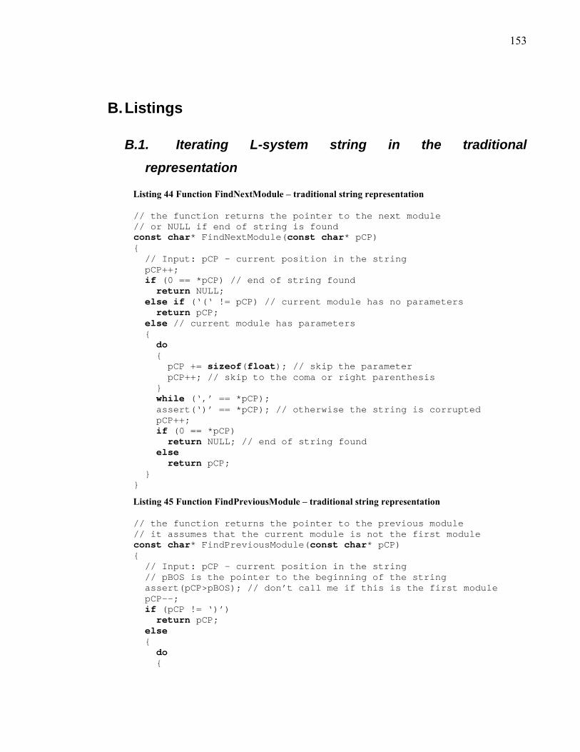
153
B. Listings
B.1. Iterating L-system string in the traditional
representation
Listing 44 Function FindNextModule � traditional string representation
// the function returns the pointer to the next module // or NULL if end of string is found const char* FindNextModule(const char* pCP) { // Input: pCP – current position in the string pCP++; if (0 == *pCP) // end of string found return NULL; else if (‘(‘ != pCP) // current module has no parameters return pCP; else // current module has parameters { do { pCP += sizeof(float); // skip the parameter pCP++; // skip to the coma or right parenthesis } while (‘,’ == *pCP); assert(‘)’ == *pCP); // otherwise the string is corrupted pCP++; if (0 == *pCP) return NULL; // end of string found else return pCP; } }
Listing 45 Function FindPreviousModule � traditional string representation
// the function returns the pointer to the previous module // it assumes that the current module is not the first module const char* FindPreviousModule(const char* pCP) { // Input: pCP – current position in the string // pBOS is the pointer to the beginning of the string assert(pCP>pBOS); // don’t call me if this is the first module pCP--; if (pCP != ‘)’) return pCP; else { do {

154
pCP -= sizeof(float); // skip the parameter pCP--; // skip to the coma or left parenthesis } while (‘,’ == *pCP); assert(‘(‘ == *pCP); // otherwise the string is corrupted pCP--; return pCP; } }
B.2. Iterating L-system string in the new representation
Listing 46 Function FindNextModule � new string representation
const char* FindNextModule(const char* pCP) { // Input: pCP – current position in the string short int ModuleId; // retrieve the current module id memcpy(&ModuleId, pCP, sizeof(short int)); // get the size of its parameters int SizeOfParameters = GetParametersSize(ModuleId); if (SizeOfParameters==0) // no parameters { pCP += sizeof(short int); // just skip the module id return pCP; } else { pCP += sizeof(short int); // skip the module id pCP += SizeOfParameters; // skip the parameters pCP += sizeof(short int); // skip the trailing id return pCP; } }
Listing 47 Function FindPreviousModule � new string representation
const char* FindPreviousModule(const char* pCP) { assert(pCP>pBOS); // don’t call me if this is the first module // skip to the previous module id pCP -= sizeof(short int); short int ModuleId; // retrieve the previous module id memcpy(&ModuleId, pCP, sizeof(short int)); // get the size of its parameters int SizeOfParameters = GetParametersSize(ModuleId); if (SizeOfParameters==0) return pCP; // no parameters – we’re done else { pCP -= SizeOfParameters; // skip the parameters pCP -= sizeof(short int); // skip the module id

155
return pCP; } }
B.3. Predefined types provided by lpfg in the file lintrfc.h template <typename f> struct V2 { V2() : x(0.0f), y(0.0f) {} V2(f nx, f ny) : x(nx), y(ny) {} V2<f> operator+(V2<f> l, V2<f> r) { return V2<f>(l.x+r.x, l.y+r.y); } // Multiplication of vector by a scalar V2<f> operator*(f r, V2<f> l) { return V2<f>(l.x*r, l.y*r); } // Scalar product f operator*(V2<f> l) { return x*l.x + y*l.y; } f x, y; }; typedef V2<float> V2f; typedef V2<double> V2d; template <typename f> struct V3 { V3() : x(0.0f), y(0.0f), z(0.0f) {} V3(f nx, f ny, f nz) : x(nx), y(ny), z(nz) {} V3<f> operator+(V3<f> l, V3<f> r) { return V3<f>(l.x+r.x, l.y+r.y, l.z+r.z); } V3<f> operator-(V3<f> l, V3<f> r) { return V3<f>(l.x-r.x, l.y-r.y, l.z-r.z); } // Multiplication of vector by a scalar V3<f> operator*(f r, V3<f> l) { return V3<f>(l.x*r, l.y*r, l.z*r); } // Scalar product f operator*(V3<f> r, V3<f> l) { return r.x*l.x + r.y*l.y + r.z*l.z; } // Vector product V3<f> operator%(V3<f> r, V3<f> l) { return V3<f>( r.y*l.z-r.z*l.y, r.z*l.x-r.x*l.z, r.x*l.y-r.y*l.x); } V3<f> operator+=(V3<f> l) {

156
x += l.x; y += l.y; z += l.z; return *this; } f x, y, z; }; typedef V3<float> V3f; typedef V3<double> V3d;

157
References [Abe1982] Abelson H., diSessa A. A. Turtle geometry. M.I.T. Press, Cambridge, 1982.
[Bat1995] Battjes J., Prusinkiewicz P. Modeling meristic characters of Asteracean
flower head. In: Symmetry in Plants (World Scientific Series in
Mathematical Biology and Medicine, Vol. 4). Jean R.V., Barabe D. (editors).
1998
[Ber1997] Berntson G. M. Topological scaling and plant root system architecture:
developmental and functional hierarchies. New Phytologist 135 (1997), pp.
621-634
[Blo1985] Bloomenthal J. Modeling the mighty maple. Proceedings of SIGGRAPH �94,
pp. 305-311, New York 1984
[Bor1984] Borchert R., Honda H. Control of development in the bifurcation branch
system of Rabebuia rosea: A computer simulation. Botanical gazette 145
(1984) 2, pp. 184-195.
[Bor1995] Borovikov I.A., L-systems with Inheritance: An Object-Oriented Extension
of L-systems. SIGPLAN Notices 30 (5), pp. 43-60, 1995
[DeK1987] De Koster C.G., Lindenmayer A. Discrete and continuous models for
heterocyst difference in growing filaments of blue-green bacteria. Acta
Biotheorica 36 (1987), pp. 247-273
[Ers2002] Erstad K. A. L-systems, Twining Plants, Lisp, Candidate Scientist thesis,
University of Bergen, Norway, 2002.
[Fed1999] Federl P., Prusinkiewicz P. Virtual Laboratory: An interactive software
environment for computer graphics. Proceedings of Computer Graphics
International 1999, pp. 93-100, 242
[Fol1990] Foley J.D., van Dam A., Feiner S., Hughes J. Computer graphics: Principles
and practice. Addison-Wesley, 1990
[Gia1997] Giavitto J.-L., DeVito D., Micehl O. Semantics and compilation of Recursive
and Sequential Streams in 8 ½. 9th International Symposium on

158
Programming Languages, Implementations, Logics and Programs
(PLILP�97), Southampton, Springer-Verlag, 1997
[Han1992] Hanan J. S. Parametric L-systems and their application to the modeling and
visualization of plants. PhD thesis, University of Regina, Canada, 1992.
[Hog1974] Hogeweg P., Herper B. A model study on biomorphological description.
Pattern Recognition 6 (1974), pp. 165-179.
[Jir2000] Jirasek C. A biomechanical model of branch shape in plants expressed using
L-systems. M. Sc. Thesis, University of Calgary, 2000
[Jir2000a] Jirasek C., Prusinkiewicz P., Moulia B. Integrating biomechanics into
developmental plant models expressed using L-systems. H.-Ch. Spatz and T.
Speck, Plant Biomechanics, Georg Thieme Verlag 2000
[Lie1986] Lieberman H. Using prototypical objects to implement shared behavior in
object-oriented systems. Proceedings of the ACM Conference on Object-
Oriented Programming Systems, Languages and Applications, pp. 214-223.
ACM, New York 1986
[Lin1968] Lindenmayer A. Mathematical models for cellular interaction in
development, Parts I and II. Journal of Theoretical Biology. 18 (1968), pp.
280-315
[Lin1971] Lindenmayer A. Developmental systems without cellular interaction, their
languages and grammars. Journal of Theoretical Biology 30 (1971), pp. 455-
484
[Lin1998] Lintermann B. Deussen O. xfrog 2.0, www.greenworks.de. December 1998.
[Lin1999] Lintermann B. Deussen O. Interactive Modeling of Plants, IEEE Computer
Graphics and Applications 19 (1), pp. 56-65, 1999.
[Mec1996] Mĕch R. Prusinkiewicz P. Visual models of plants interacting with their
environment. Proceedings of SIGGRAPH �96. ACM SIGGRAPH, New York
1996, pp. 397-410
[Mec1997] Mĕch R. Modeling and simulation of the interactions of plants with the
environment using L-systems and their extensions. PhD thesis, University of
Calgary, 1997

159
[Mec1997a] Mĕch R., Prusinkiewicz P., Hanan J. Extensions to the graphical
interpretation of L-systems based on turtle geometry. Unpublished
manuscript.
[Mec1998] Mĕch R. Cpfg version 3.4. User�s Manual.
http://www.cpsc.ucalgary.ca/Research/bmv/lstudio/manual.pdf.
[Mer1990] Mercer L., Prusinkiewicz P., Hanan J. The concept and design of a virtual
laboratory. Proceedings of Graphics Interface �90, pp. 149-155. CIPS 1990
[Mer1991] Mercer L. The virtual laboratory. Master�s thesis, University of Regina,
1991
[Pow1999] Power J. L., Bernheim Brush A. J., Salesin D., Prusinkiewicz P. Interactive
arrangement of Botanical L-system Models, 1999 ACM Symposium on
Interactive 3D Graphics
[Pru1986] Prusinkiewicz P. Graphical applications of L-systems. Proceedings Graphics
Interface 1986.
[Pru1987] Prusinkiewicz P. Applications of L-systems to computer imagery. Graph
grammars and their application to computer science; Third International
Workshop, editors: H. Ehrig, M. Nagl, A. Rosenfeld, G Rozenberg.
Springer-Verlag, Berlin, 1987. Lecture Notes in Computer Science 291, pp.
534-548.
[Pru1988] Prusinkewicz P., Lindenmayer A., Hanan J. Developmental models of
herbaceous plants for computer imagery purposes. Proceedings of
SIGGRAPH �88. ACM SIGGRAPH, New York, 1988
[Pru1990] Prusikniewicz P,. Lindenmayer A. The algoritrhmic beauty of plants.
Springer-Verlag, New York, 1990
[Pru1992] Prusinkiewicz P., Hanan J. L-systems: From formalism to programming
languages. Lindenmayer systems: Impact on theoretical computer science,
computer graphics, and developmental biology, G. Rozenberg and A.
Saloma, Springer-Verlag, Berlin 1992, pp. 193-211
[Pru1994] Prusinkiewicz P., James M., Mĕch R. Synthetic topiary. Proceedings of
AIGGRAPH �94. ACM SIGGRAPH, New York 1994, pp. 351-358

160
[Pru1996] Prusinkiewicz P., Hammel M., Hanan J., Mĕch R. L-systems: from the theory
to visual models of plants. Machine Graphic and Vision 5 (1996), pp. 365-
392
[Pru1997] Prusinkiewicz P., Mĕch R. Application of L-systems with homomorphism to
graphical modeling. University of Calgary, Calgary, Canada 1997.
Manuscript.
[Pru1997a] Prusinkiewicz P., Hammel M., Hanan J., Mĕch R. Visual Models of Plant
Development. In G. Rozenberg and A. Salomaa (Eds.): Handbook of Formal
Languages Vol III, Springer, Berlin 1997, pp. 535-597.
[Pru1999] Prusinkiewicz P., Karwowski R., Mĕch R., Hanan J. L-studio/cpfg: a
software system for modeling plants. Lecture Notes in Computer Science
1779: Applications of graph transformation with industrial relevance, pp.
457-464.
[Pru2001] Prusinkiewicz P., Mündermann L., Karwowski R., Lane B. The Use of
Positional Information in the Modeling of Plants. Proceedings of
SIGGRAPH 2001, pp. 289-300.
[Pru2002] Prusinkiewicz P., Samavati F., Smith C., Karwowski R. L-system description
of subdivision curves. University of Calgary, June 2002. Submitted for
publication.
[Roo1996] Room P., Hanan J., Prusinkiewicz P. Virtual plants: New perspectives for
ecologists, pathologists and agricultural scientists. Trends in Plant Science.
1, pp. 33-38
[Roz1980] Rozenberg G., Saloma A. The mathematical theory of L-systems. Academic
Press, New York, 1980
[Shi1964] Shinozaki K., Yoda K., Hozumi K., Kira T. A quantitative analysis of plant
form � the pipe model theory. Japanese Journal of Ecology, 14 (3), 1964, pp.
97-104.
[Smi1984] Smith A. R. Plants, fractals and formal languages. Proceedings of
SIGGRAPH �84. ACM SIGGRAPH New York, 1984.
[Str1991] Stroustroup B. The C++ Programming Language, Addison-Wesley, 1991

161
[Vog1979] Vogel H. A better way to construct the sunflower head. Mathematical
Biosciences, 44 (1979), pp. 179-189.
[Wad1942] Waddington C. H. Canalization of development and the inheritance of
acquired characteristics. Nature, 150, pp. 563-565, 1942.
[Woo1999] Woo M., et al. OpenGL Programming Guide: The Official Guide to
Learning OpenGL (3rd Edition). Addison-Wesley, 1999