Indoor positioning in LoRaWAN networks

Evaluation of RSS positioning in LoRaWAN networks usingcommercially available hardware

Master’s thesis in Communication Engineering

RASMUS HENRIKSSON

Department of Signals and SystemCHALMERS UNIVERSITY OF TECHNOLOGYGöteborg, Sweden 2016

Master’s thesis 2016:45

Indoor positioning inLoRaWAN networks

Evaluation of RSS positioning in LoRaWAN networks usingcommercially available hardware

RASMUS HENRIKSSON

Department of Signals and SystemsDivision of Communication systems

Chalmers University of TechnologyGöteborg, Sweden 2016

Indoor positioning in LoRaWAN networksEvaluation of RSS positioning in LoRaWAN networks using commercially availablehardwareRASMUS HENRIKSSON

© Rasmus Henriksson, 2016.

Examiner: Henk Wymeersch, Signals and Systems

Master’s Thesis 2016:45Department of Signals and SystemsDivision of Communication SystemsChalmers University of TechnologySE-412 96 GothenburgTelephone +46 31 772 1000

Göteborg, Sweden 2016

Indoor positioning in LoRaWAN networksEvaluation of RSS positioning in LoRaWAN networks using commercially availablehardwareRASMUS HENRIKSSONDepartment of Signals and SystemsChalmers University of Technology

iv

AbstractAs the Internet of Things expands, new networks are launched in order to providelong range links with low power usage. While the low power consumption is one ofthe key components of devices connected to these networks, low cost is another whichallows for large scale deployments of devices. By providing a position estimationbuilt into these networks both power and cost can be cut by not having to useany GNSS solution. This thesis investigates if the received signal strength fromLoRaWAN networks can be used to determine the position of a connected end-device. The study is done by simulating a large scale network with real worldmeasurements to study how the number of anchor nodes impact the positioningaccuracy. Results show that the measurements vary too much to give a good positionestimation.

v

AcknowledgementsThis work is the final part in my master’s program Communication Engineering atChalmers University of Technology. The work have been conducted for Cybercomat their Gothenburg office.I would like to thank Gabriel Ibanez and Henrik Lundqvist at Cybercom for trustingme with this task and their support along the way. I would also like to thank HenkWymeersch for being my examiner and helping to point me in the right directionduring the project.

Rasmus Henriksson, Göteborg, June 2016

vi

Contents

1 Introduction 11.1 Low-Power Wide-Area Networks . . . . . . . . . . . . . . . . . . . . . 11.2 Indoor positioning in research . . . . . . . . . . . . . . . . . . . . . . 21.3 Outline of project . . . . . . . . . . . . . . . . . . . . . . . . . . . . . 31.4 Thesis outline . . . . . . . . . . . . . . . . . . . . . . . . . . . . . . . 3

2 LoRaWAN 52.1 Organisation . . . . . . . . . . . . . . . . . . . . . . . . . . . . . . . . 52.2 Modulation . . . . . . . . . . . . . . . . . . . . . . . . . . . . . . . . 52.3 Network structure . . . . . . . . . . . . . . . . . . . . . . . . . . . . . 6

3 Positioning 93.1 Positioning basics . . . . . . . . . . . . . . . . . . . . . . . . . . . . . 93.2 Received Signal Strength . . . . . . . . . . . . . . . . . . . . . . . . . 103.3 Time of Arrival . . . . . . . . . . . . . . . . . . . . . . . . . . . . . . 113.4 Calculating position estimates . . . . . . . . . . . . . . . . . . . . . . 11

4 Implementation 134.1 Network setup . . . . . . . . . . . . . . . . . . . . . . . . . . . . . . . 134.2 Gathering RSS measurements . . . . . . . . . . . . . . . . . . . . . . 144.3 Simulation . . . . . . . . . . . . . . . . . . . . . . . . . . . . . . . . . 15

5 Results and discussion 175.1 Indoor measurements . . . . . . . . . . . . . . . . . . . . . . . . . . . 175.2 Simulation results . . . . . . . . . . . . . . . . . . . . . . . . . . . . . 195.3 Measurement and simulation interpretations . . . . . . . . . . . . . . 205.4 Time of arrival or received signal strength . . . . . . . . . . . . . . . 215.5 Positioning algorithm . . . . . . . . . . . . . . . . . . . . . . . . . . . 22

6 Conclusion 23

Bibliography 25

A End-device source code I

vii

Acronyms

3GPP 3G Partnership ProgramADR Adaptive Data RateAoA Angle of ArrivalBW BandwidthdBm Decibell milliwattDL DownlinkFHSS Frequency-Hopping Spread SpectrumFPGA Field-Programmable Gate ArrayFSK Frequency Shift KeyingGNSS Global Navigation Satellite SystemIID Independent and Identically DistributedIoT Internet of ThingsISM Industrial, scientific and medical (radio bands)LBT Listen Before TalkLLS Linearised Least Squares (method)LoRa Long Range (modulation technique)LoRaWAN Long Range Wide Area Network (network standard)LOS Line Of SightLPWAN Low Power Wide Area NetworkM2M Machine to machine (communication)MAC Medium Access ControlML Maximum LikelihoodRMS Root Mean SquareRSS Received Signal StrengthSF Spread FactorSNR Signal-to-Noise RatioToA Time of ArrivalUL UplinkWAN Wide Area NetworkWSN Wireless Sensor Network

viii

1Introduction

In the year 2016 everything seem to revolve around the emergence of IoT, whereanything from cars to bathroom scales is to be connected to the internet in orderto provide additional services for the consumer. However, the driving force behindIoT is more likely to be industry applications evolving from M2M technologies.Speaking in broad terms, IoT is simply an evolution of M2M communications, wheremore emphasis is put on connecting large number of nodes and using an ethernetback-end to reroute data as needed. This is a crucial step towards building smartcity applications and what is called the fourth industrial revolution, where expertsanticipate that the borders between what is physical, digital and biological willbecome blurred in industries [1]. With such a large scale goal and a lack of existinginfrastructure to power it, companies are fighting to launch their own solution fornetworks supporting the IoT. While many M2M applications relied on 2G for largescale deployment, or smaller local networks for indoor, the IoT revolution sees theemergence of networks with different requirements, such as low chip-cost and supportfor tens of thousands of nodes in a single cell. Right now there are a lot of upcomingnetwork standards that promise to solve these and many other issues. Among themost discussed competitors are Sigfox, LoRaWAN and LTE-M. This thesis will focuson the network standard called LoRaWAN, within the subset of networks dealingwith long-range and low-power applications.

1.1 Low-Power Wide-Area Networks

LPWAN is an acronym for Low-power Wide-Area Networks, which as the namesuggests, focus on providing large cells for low-power end-devices, typically batterypowered. The main driving force is to provide network access for M2M and IoTapplications over large distances, but still maintaining a low power consumption.On top of this, many companies are competing to provide cheap and easy-to-installsolutions, making for quite a challenging task.As range, power and bandwidth are closely related factors in networks, changing oneof these will inevitably have an impact on the other two. In the case of LPWANs,the bandwidth is sacrificed in order to ensure a low-power communication over longrange. What the terms ’low’ and ’long’ refers to in this context is not clearly defined,but a typical LPWAN have a range of about 10 km, an expected battery life forend-devices of 5-10 years and a maximum bit rate around 1-50 kpbs.

1

1.1.1 LoRaWAN and CompetitorsCurrently there are several LPWAN standards developed by different organisations.Of these LoRaWAN, Sigfox, NB-IoT, LTE-M and Weightless are probably the onesmost often heard of. While there are large differences in how the standards arebuilt in term of modulation, bit rate etc, the main differences are probably in thedifferent business models [2]. Notably LoRaWAN and Weightless are both developedas open standards in unlicensed spectrum, meaning that anyone can set up theirown network if desired. This opens up for interesting dynamics in a business areadominated by mobile network operators. On the other end of the spectrum, Sigfoxis a company acting as both developer and operator, who are aiming for worldwidenetwork support.The last two standards, NB-IoT and LTE-M, are both standardized by 3GPP anddeveloped in the traditional way that has formed the latest cellular network stan-dards. The aim for these techniques are to provide a standard for network operatorto deploy in licensed spectrum on top of existing 4G network. Additionally theevolution of 5G aims to target IoT applications as well, but as it is still in an earlydevelopment stage it will not be considered further at this point in time.

1.2 Indoor positioning in researchIn IoT in general, and particularly in wireless sensor networks, a core issue is powerconsumption and cost of modules. By deploying an internal positioning techniquein the network instead of using a GNSS based technique, both of these factors canbe kept to a minimum. Moreover many of these networks are intended for indooruse, eliminating the use of GNSS at all because they lack the required Line-of-Sight(LOS).In current research there have been quite a few attempts to solve the problem ofindoor positioning with sufficient accuracy with varying results. While there arecommercial systems such as the iBeacon and WiFiSLAM from Apple they are oftento crude to be used in industry, and are mainly developed for use in advertisement.In research however, WiFi has been used with an accuracy of 1m when using acombination of ToA/AoA (Time of Arrival, Angle of Arrival) and multiple precodedmessages. By spacing these messages over the sample time in the receiver, a goodestimation of the position can be calculated with existing hardware [3]. A comple-mentary standard is Bluetooth Low Energy (BLE), where the main algorithm usedis fingerprinting with beacons as anchor nodes [4]. With fingerprinting a heat mapof the signal strength is constructed for the area in which the positioning algorithmis to be used. While this yields good results, the map will degrade over time andneeds to be updated continuously.

2

1.3 Outline of project

1.3.1 PurposeThe purpose of this thesis is two-fold. The first is to make use of the LoRaWANnetwork standard to set up a functioning network. This network will then be usedto gather measurements in order to simulate how a large-scale deployment wouldprovide indoor positioning estimates. With this simulation, different aspects on howa positioning algorithm using LoRaWAN would function will be evaluated.

1.3.2 ObjectiveThe objective of the thesis can be summarised as the four goals:

• To learn and utilise the open network standard LoRaWAN• To build a functioning LoRaWAN network to use for gathering of measure-

ments• Simulate a positioning algorithm as a proof-of-concept• Evaluate the accuracy of the positioning system, and suggest improvements

for further studies

1.3.3 ScopeThe project is set to deliver a positioning method using existing LoRaWAN hard-ware. The method is intended as a proof-of-concept, and therefor aspects such ascost and battery consumption are disregarded.

1.4 Thesis outlineThe thesis is divided into six chapters including this one. Chapter 2 will explainhow the LoRaWAN standard functions, and elaborate on how the modulation calledLoRa is a vital part of this network standard.Chapter 3 will go through the basics of wireless position techniques. It will also relatethese techniques to the LoRaWAN standard and evaluate which are of interest forthe research question.Chapter 4 describes the methods used for each step of the project. The hardwareof the network is presented, how measurements were conducted and finally how thesimulation was carried out.Chapter 5 will present the results of both measurements and simulation, along witha discussion on interpretations. Improvements and fault sources will also be dealtwith in this chapter.Finally, chapter 6 will present a conclusion and suggestions for how further researchcan be conducted on this subject.

3

4

2LoRaWAN

LoRaWAN is an LPWAN developed and maintained by the LoRa Alliance. Thisstandard builds upon the LoRa modulation developed by Semtech and adds a net-work layer to handle traffic between end-devices and central nodes. This allowsfor communication over long range for low data-rate devices. The main motivationbehind the network is to enable IoT, wide-area sensor networks, and other M2Mapplications. For the current release (v1.1), the focus of the network is on uplinkcommunications.

2.1 Organisation

The LoRaWAN standard is developed by a non-profit organization called the LoRaAlliance. The LoRa Alliance include over 200 companies as of June 2016, whichspan the whole LoRaWAN ecosystem. The organisation is split around sponsors,contributors, institutional members and adopters, where the first three categoriesmainly work with development, and the last is certified to sell LoRa-compatibleproducts. Initially the LoRa standard, short for Long Range, was developed by aFrench startup called Cycleo in 2012, which was later acquired by Semtech. Semtechalso founded the LoRa Alliance together with companies such as Microchip, IBMand Cisco with the goal of creating a network standard using the LoRa modulation.Currently Semtech is the owner of two patents used in the LoRa chipset, FractionalN-synthesized chirp generator [5] and Low power long range transmitter [6], whichmakes Semtech a key player in the LoRa Alliance.

2.2 Modulation

The key enabling factor in LoRaWAN networks is the LoRa modulation standard.The LoRa modulation uses a proprietary Chirp Spread Spectrum (CSS) scheme,which creates wideband linear frequency modulated chirps. The chip rate of thesechirps are equal to the spectral bandwidth of the signal and uses 125, 250 or 500kHz of bandwidth. The gains of using using CSS are twofold, the first being thatchirps are noise resistant and the second that these chirps can be generated withhigh precision using a cheap crystal, which leads to low chip costs. Because of therelative broadband characteristics of the chirps, multi-path fading is typically notan issue [7]. Doppler spread causes a frequency shift, which also only have a smalleffect on the channel thanks to the time-varying frequency of the chirps. When

5

0 2 4 6 8 10 12 14 16 18

Time

-1

-0.5

0

0.5

1

Am

plitu

de

Figure 2.1: Visualisation of the up-chirps used in the LoRa modulation. Thefrequency increases as a linear function of time.

using the LoRa modulation, 15 km of range can be achieved in urban environmentsand up to 30 km with good line-of-sight [7].Additionally LoRa uses a Frequency-Hopping Spread Spectrum (FHSS) scheme toswitch frequency between available channels according to a pseudo-random distri-bution. This helps to further mitigate interference.A key thing to note with the CSS modulation scheme is that it produces a verysharp peak when auto-correlated, and has previously been deployed in radar ap-plications [8]. The high peak helps to identify the correct time that the signal isreceived, and thus can be used to give a good estimate of the time it takes for atransmission to travel between two nodes.

2.2.1 Symbol coding and bit rateThe bit rate of LoRa varies between 0.3 and 22 kpbs depending on the spreadfactor used. The spread factor can take on values between 7 and 12, and each ofthese are associated with a set of orthogonal codes which allows for simultaneouscommunication at different bit rates. Symbol coding in LoRa is accomplished byusing time-shifted up-chirps which are interleaved to improve robustness [9]. Byusing a higher spreading factor, the robustness of the communication link is increasedbut as a consequence the time-on-air also increases.

2.3 Network structureThe LoRaWAN network protocol is a standard developed by the LoRa Alliance.The first version was released in 2015, and the current version as of June 2016 is1.1. The network uses the terminology gateways, end-devices and network serverto distinguish between different entities. The end-devices are typically some kindof sensor, which are further divided into three different categories depending on

6

Figure 2.2: Sketch of a typical LoRaWAN network setup.

their power consumption. The end-devices are connected to gateways in a startopology, where the gateway is the central node. Typically a gateway can handleseveral thousands of end-devices, however they do not communicate directly withother gateways. Instead gateways are connected by ethernet to the network server,which stores data and handles traffic in both directions. This makes for a star-of-star topology where the network server is the central node, and gateways areintermediate nodes. As LoRaWAN operates in unlicensed ISM bands, gateways aretypically set up by both companies and private users. Currently there are a fewcrowdsourced networks such as The Things Network. In these networks users sharea network server provided by a company, and gateways are crowdfunded locally andopen to use for anyone who own LoRa compatible end-devices.

2.3.1 Device classesLoRaWAN devices are divided into three different classes depending on their in-tended load on the network. All devices must have at least Class A functionality tobe considered LoRa certified devices. Restrictions for Class A devices are to opentwo receive windows following each uplink transmission. In practice this means thatthe device can be inactive for long periods of time to conserve battery power. Theonly way for the gateway to communicate downlink with the end-device is to waitfor an uplink transmission and then respond.Class B devices have, on top of Class A functionality, dedicated time slots for re-ceiving downlink messages, and also periodically receives beacon messages for clocksynchronisation. Class C devices are continuously listening, and are therefore in-tended to be connected to a power supply.

2.3.2 License-free carrierThe LoRa modulation is built around using a license-free carrier frequency whichvaries between different regions of the world. Currently there are standards forEurope, US and China which span certain ranges within 433-870 MHz. All of theused carrier frequencies in LoRaWAN are ISM bands. For Europe, 863-870 MHz isthe most common band used, which will also be used in the studies in this project.Because LoRaWAN is not based on a Listen Before Talk (LBT) principle, there arecertain restrictions limiting the duty cycles between 0.1-10% depending on whichband is used.

7

8

3Positioning

Positioning is crucial for many LPWAN applications due to the nature of the datagathered. Specially as the number of devices can range up to several thousandswithin a single cell, estimating position is of vital importance in order to install anduse data from end-devices properly. An example of this is using temperature sensorsto measure temperature fluctuations in an urban area. As the number of temper-ature sensors increase, so will the accuracy of the city’s temperature distributionmodel. However, when using a large number of sensors it will become tedious andexpensive work to manually program the position of each sensor.A natural solution to this problem would be to equip each sensor with a GNSStracker, for example using GPS. While this solution is tempting, adding a GPStracker to a device will increase both cost and power consumption [10]. Anotherissue with using a satellite based system is the lack of indoor coverage, which doesnot only include offices and home, but also factories and malls. Taking this intoconsideration, speculation can be made that the LPWAN to be used in the future isthe one which first can introduce a reliable positioning system which uses low powerand works indoor.

3.1 Positioning basics

In this chapter the terminology anchor nodes will be used to describe nodes with ana priori known location and target nodes are nodes with unknown position whichwill have their position estimated. To simplify calculations, all nodes are consideredto exist in a 2-dimensional plane and thus in a real-world scenario this correspondsto all nodes being located at the same altitude.To find the position of target nodes one must first identify which measurable param-eters are of interest, and then link these parameters mathematically to the distancebetween anchor and target nodes. Typically these are the received signal strength(RSS), ToA or Aoa, which can be utilised in a variety of different ways to calculatethe distance between nodes. As AoA requires antenna arrays to function, which isnot supported in the LoRaWAN specification as of now, it will not be consideredfurther.When RSS or ToA are used, the most simple approach to visualise the system ofequations is that shown in equation (3.1), where pi is the position of anchor nodes,pt the position of the single target node, and vi is the measurement error associatedwith the distance between pi and pt. Note that vi is a random variable, which isassumed to be zero-mean [11]. The real properties of vi can be obtained by executing

9

test runs where pt is known.

|pi − pt| =√

(xi − xt)2 + (yi − yt)2 + vi (3.1)pi = (xi, yi), i = 1, .., na

pt = (xt, yt)(3.2)

To solve equation (3.1) the task is to maximise the probability density functionp(pt|pt) where pt is the estimated position given by measurements. This can eitherbe done in non-iterative ways such as linearised least squares method, or by usingan iterative filtering function suitable for non-linear equations such as an extendedor linearised Kalman filter. For the sake of estimating the positioning accuracy, themore simple method of least squares estimation will be used in this project.

3.2 Received Signal StrengthAs wireless signals traverse air they are subject to several effects causing signaldegradation. Usually these are described as a sum of a second-order function anda random variable which describes time and frequency related fluctuations. In thesimplest case scenario, the power received Pr is related to the power transmitted,Pt, through the free space path loss model described in equation (3.3). The FSPLmodel consider only LOS connections, and model these as deterministic processes.

Pr = Pt

(√GrGtλ

4πd

)2

(3.3)

Which rewritten in decibel scale becomes the following equation:

Pr[dBm] = Pt[dBm]− 20 log10(d)− 20 log10(4πλ

) (3.4)

Through the free space path loss model it is clear that the power received dependsnot only on the distance between nodes, but also the antenna gain, G, and thewavelength of the carrier signal, λ. Through empirical studies the FPSL modelhave evolved into what is known as the log-distance path loss model, where theunknown parameters are determined through experiments [11]. The parameters aredetermined at a reference distance, d0, and clump together into a single parameter,PL0 as seen in equation (3.5). Please note that all power units will be in the dBmscale from now onwards.

Pr = Pt − PL0 − 10γ log10

( dd0

)(3.5)

Here γ denotes the path loss exponent, and varies depending on environment andhardware setup. In the previous FSPL model this exponent is equal to 2.The last piece in the RSS equation is the shadowing effect, denoted Xg, which is arandom variable to describe fluctuations in measurements caused by various distur-bances such as interference from other transmissions, weather effects or scattering.

10

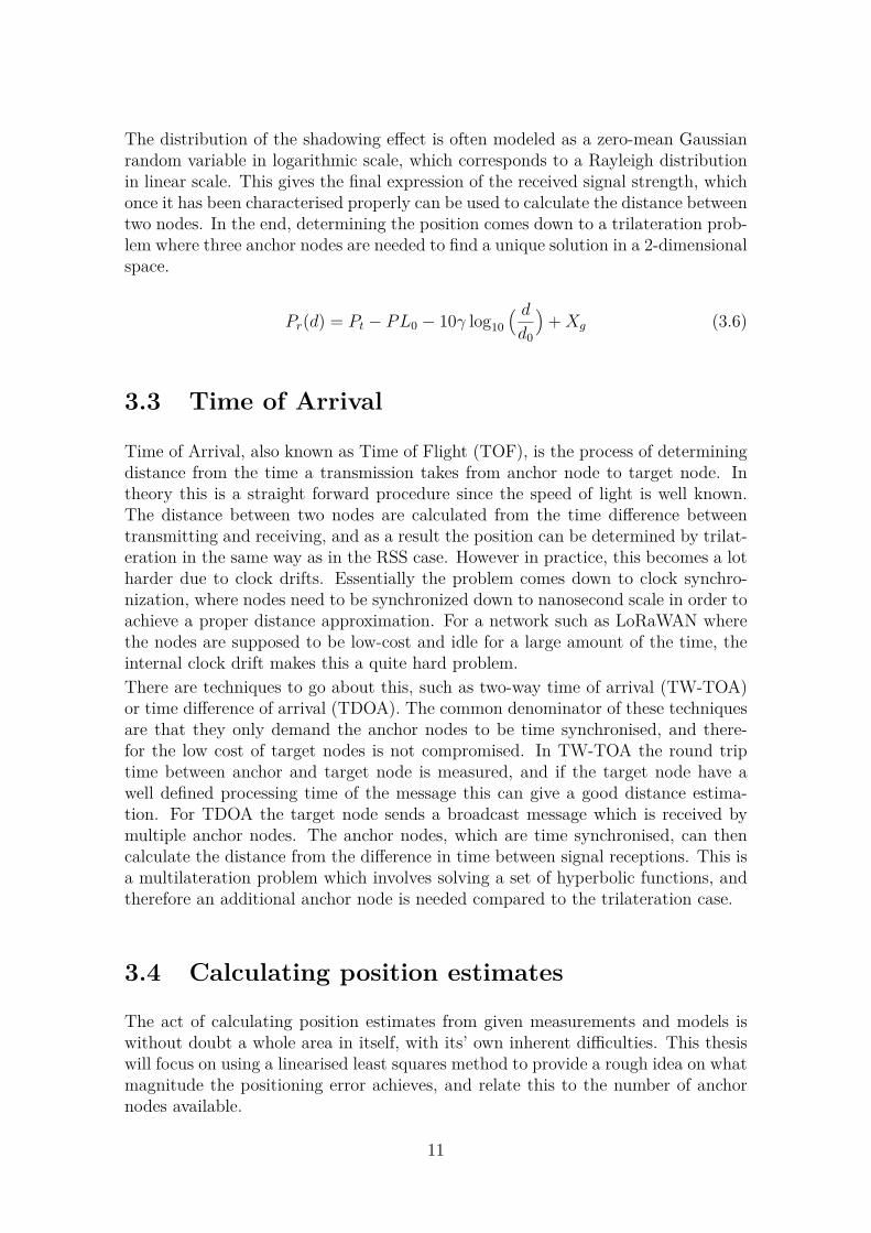
The distribution of the shadowing effect is often modeled as a zero-mean Gaussianrandom variable in logarithmic scale, which corresponds to a Rayleigh distributionin linear scale. This gives the final expression of the received signal strength, whichonce it has been characterised properly can be used to calculate the distance betweentwo nodes. In the end, determining the position comes down to a trilateration prob-lem where three anchor nodes are needed to find a unique solution in a 2-dimensionalspace.

Pr(d) = Pt − PL0 − 10γ log10

( dd0

)+Xg (3.6)

3.3 Time of Arrival

Time of Arrival, also known as Time of Flight (TOF), is the process of determiningdistance from the time a transmission takes from anchor node to target node. Intheory this is a straight forward procedure since the speed of light is well known.The distance between two nodes are calculated from the time difference betweentransmitting and receiving, and as a result the position can be determined by trilat-eration in the same way as in the RSS case. However in practice, this becomes a lotharder due to clock drifts. Essentially the problem comes down to clock synchro-nization, where nodes need to be synchronized down to nanosecond scale in order toachieve a proper distance approximation. For a network such as LoRaWAN wherethe nodes are supposed to be low-cost and idle for a large amount of the time, theinternal clock drift makes this a quite hard problem.There are techniques to go about this, such as two-way time of arrival (TW-TOA)or time difference of arrival (TDOA). The common denominator of these techniquesare that they only demand the anchor nodes to be time synchronised, and there-for the low cost of target nodes is not compromised. In TW-TOA the round triptime between anchor and target node is measured, and if the target node have awell defined processing time of the message this can give a good distance estima-tion. For TDOA the target node sends a broadcast message which is received bymultiple anchor nodes. The anchor nodes, which are time synchronised, can thencalculate the distance from the difference in time between signal receptions. This isa multilateration problem which involves solving a set of hyperbolic functions, andtherefore an additional anchor node is needed compared to the trilateration case.

3.4 Calculating position estimates

The act of calculating position estimates from given measurements and models iswithout doubt a whole area in itself, with its’ own inherent difficulties. This thesiswill focus on using a linearised least squares method to provide a rough idea on whatmagnitude the positioning error achieves, and relate this to the number of anchornodes available.

11

3.4.1 Non-iterative algorithm: Linearised Least-Squares

Let di be the distance between anchor node i and the target node, and di theestimated distance. The relationship between these two variables can be describedby equation (3.7) where vi is an unknown random variable corresponding to thepositioning error. By writing out the vectors dt and di as their x− and y-coordinatesit is clear that this is not a linear equation and will need some type of linearisationin order to be used in a least-square sense. By evaluating the squares introduced inthe previous step, equation (3.9) is found.

di = di + vi (3.7)(di − vi)2 = (xi − xt)2 + (yi − yt)2 (3.8)

(x2t + y2

t )− 2(xixt + yiyt) = (di − vi)2 − (x2i + y2

i ) (3.9)

This equation is rewritten by introducing the variables Ri and Rt as the nodes’ radiifrom origo. This gives equation (3.11).Rt =

√x2

t + y2t

Ri =√x2

i + y2i

⇒ R2t − 2(xixt + yiyt) = d2

i − 2divi + v2i −R2

i (3.10)d2

i −R2i = −2xixt − 2yiyt +R2

t + 2dini − n2i (3.11)

The final step is now to rewrite this as a linear system, which is done with vectornotation in equation (3.12). The j-index denotes row j of the matrix.

h = Gθ + n (3.12)where θ = [x, y, R2]T

Gj = [−2xi, −2yi, 1]hj = [d2

i −R2i ]

nj = [v2i − 2divi]

(3.13)

Since this equation is linear, the least-square estimator is known as

θ =(GT WG

)−1GT Wh (3.14)

The price to pay for linearisation is that the measurement noise v is squared toproduce n. Assuming that v is a zero-mean variable this should still produce areliable estimation.

12

4Implementation

In this chapter methods used to build the network, conduct measurements and sim-ulate position estimation will be described. Also any hardware used in the networkwill be described. For simulations, Matlab have been used.

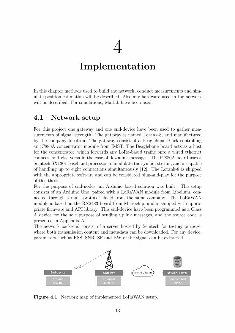
4.1 Network setupFor this project one gateway and one end-device have been used to gather mea-surements of signal strength. The gateway is named Lorank-8, and manufacturedby the company Ideetron. The gateway consist of a Beaglebone Black controllingan iC880A concentrator module from IMST. The Beaglebone board acts as a hostfor the concentrator, which forwards any LoRa-based traffic onto a wired ethernetconnect, and vice versa in the case of downlink messages. The iC880A board uses aSemtech SX1301 baseband processor to modulate the symbol stream, and is capableof handling up to eight connections simultaneously [12]. The Lorank-8 is shippedwith the appropriate software and can be considered plug-and-play for the purposeof this thesis.For the purpose of end-nodes, an Arduino based solution was built. The setupconsists of an Arduino Uno, paired with a LoRaWAN module from Libelium, con-nected through a multi-protocol shield from the same company. The LoRaWANmodule is based on the RN2483 board from Microchip, and is shipped with appro-priate firmware and API library. This end-device have been programmed as a ClassA device for the sole purpose of sending uplink messages, and the source code ispresented in Appendix A.The network back-end consist of a server hosted by Semtech for testing purpose,where both transmission content and metadata can be downloaded. For any device,parameters such as RSS, SNR, SF and BW of the signal can be extracted.

Figure 4.1: Network map of implemented LoRaWAN setup.

13

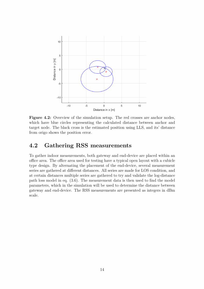
Figure 4.2: Overview of the simulation setup. The red crosses are anchor nodes,which have blue circles representing the calculated distance between anchor andtarget node. The black cross is the estimated position using LLS, and its’ distancefrom origo shows the position error.

4.2 Gathering RSS measurementsTo gather indoor measurements, both gateway and end-device are placed within anoffice area. The office area used for testing have a typical open layout with a cubicletype design. By alternating the placement of the end-device, several measurementseries are gathered at different distances. All series are made for LOS condition, andat certain distances multiple series are gathered to try and validate the log-distancepath loss model in eq. (3.6). The measurement data is then used to find the modelparameters, which in the simulation will be used to determine the distance betweengateway and end-device. The RSS measurements are presented as integers in dBmscale.

14

4.3 SimulationTo evaluate the accuracy of this positioning approach Matlab have been used to con-duct simulations where the number of anchor nodes vary. The goal of the simulationsis to put a number on how good the accuracy is for this method of positioning. Toget a rough understanding of this, a non-iterative optimisation method is used tocalculate mean and standard deviation as a function of nodes. The simulation usesfour general steps which are described below.

1. In this setup, the real position of the end-device is always at (0, 0). n gatewaysare generated at random distance and angle from origo, both drawn from auniform distribution. While the angle can have any value in the range [0, 2π],the distance may only take on discrete values which have measurement dataassociated with them. For this simulation, it is assumed that all antennas areisotropic radiators.

2. Each gateway, gi, i ∈ [1, n], is associated with an RSS value depending on thereal distance between the end-device in origo and gi. The RSS value is drawnfrom the set of actual data associated with this distance, and the index of thisvalue is from a uniform distribution.

3. The theoretical distances, di are calculated by using eq. (3.6) with the ex-tracted model parameters. This model assumes that the noise is zero-mean,and as such the true distance is associated with a random variable as in eq.(4.1).

di = di + v (4.1)

From each gateway, located at (xi, yi), a circle is drawn with radii di. A sketchof how the simulation setup looks can be found in figure 4.2.

4. The problem of finding the true position is now a non-linear optimisationproblem, where the point closest to all circles is to be found. This is solved byusing the linearised least squares method presented in equation (3.12).

15

16

5Results and discussion

This chapter will present the results found from the measurements and simulationscarried out during this project, followed by a discussion interpreting them. First themeasurement data will be presented and analysed. These measurements are thenused in the simulations presented in previous chapter. The results of these simu-lations are presented with focus on how the positioning accuracy can be increasedwith a growing number of anchor nodes. The results of these simulations are thendiscussed in the second part of this chapter.

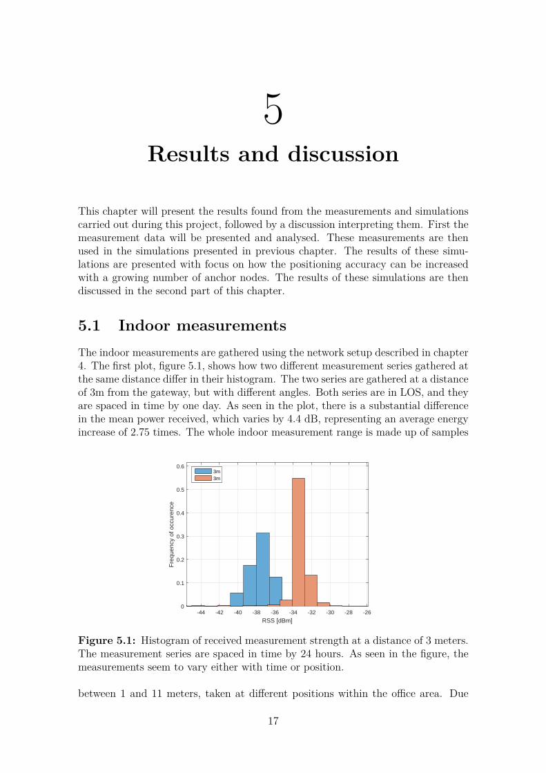
5.1 Indoor measurementsThe indoor measurements are gathered using the network setup described in chapter4. The first plot, figure 5.1, shows how two different measurement series gathered atthe same distance differ in their histogram. The two series are gathered at a distanceof 3m from the gateway, but with different angles. Both series are in LOS, and theyare spaced in time by one day. As seen in the plot, there is a substantial differencein the mean power received, which varies by 4.4 dB, representing an average energyincrease of 2.75 times. The whole indoor measurement range is made up of samples

-44 -42 -40 -38 -36 -34 -32 -30 -28 -26

RSS [dBm]

0

0.1

0.2

0.3

0.4

0.5

0.6

Fre

quen

cy o

f occ

uren

ce

3m3m

Figure 5.1: Histogram of received measurement strength at a distance of 3 meters.The measurement series are spaced in time by 24 hours. As seen in the figure, themeasurements seem to vary either with time or position.

between 1 and 11 meters, taken at different positions within the office area. Due

17

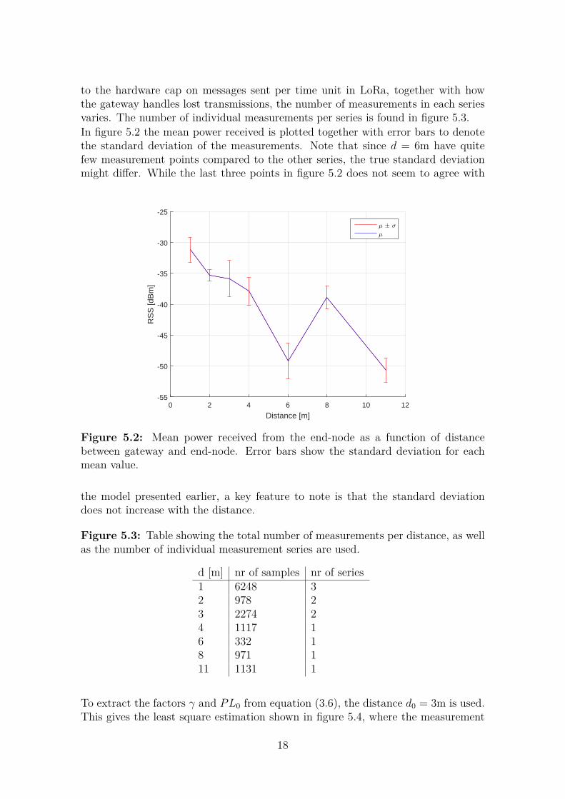
to the hardware cap on messages sent per time unit in LoRa, together with howthe gateway handles lost transmissions, the number of measurements in each seriesvaries. The number of individual measurements per series is found in figure 5.3.In figure 5.2 the mean power received is plotted together with error bars to denotethe standard deviation of the measurements. Note that since d = 6m have quitefew measurement points compared to the other series, the true standard deviationmight differ. While the last three points in figure 5.2 does not seem to agree with

0 2 4 6 8 10 12

Distance [m]

-55

-50

-45

-40

-35

-30

-25

RS

S [d

Bm

]

µ ± σµ

Figure 5.2: Mean power received from the end-node as a function of distancebetween gateway and end-node. Error bars show the standard deviation for eachmean value.

the model presented earlier, a key feature to note is that the standard deviationdoes not increase with the distance.

Figure 5.3: Table showing the total number of measurements per distance, as wellas the number of individual measurement series are used.

d [m] nr of samples nr of series1 6248 32 978 23 2274 24 1117 16 332 18 971 111 1131 1

To extract the factors γ and PL0 from equation (3.6), the distance d0 = 3m is used.This gives the least square estimation shown in figure 5.4, where the measurement

18

mean for each d is plotted with a logarithmic distance of base ten. Here, γ = 1.69and PL0 = −35.9.

-0.2 0 0.2 0.4 0.6 0.8 1 1.2

log10

d

-55

-50

-45

-40

-35

-30

-25R

SS

[dB

m]

Least square estimationµ ± σµ

Figure 5.4: RSS plotted against a logarithmic distance. The black graph is theleast square estimator of the measurements when correlated with the log distancepath loss model.

By studying the deviation of measurement values from the distance-related meanvalue, µ(d), a distribution for the shadowing effects can be found. This is done bysubtracting µ(d) from each measure point, and results in the histogram in figure5.5. From visual inspection, it is clear that the histogram bear strong resemblanceto a Gaussian distribution, however the additional peaks suggest that it is the sumof several Gaussian random variables.

5.2 Simulation results

The positioning simulation are carried out as a function of the number of nodes, n.At each i ∈ [3, n] the root mean square (RMS) error and its’ standard deviation iscalculated over 1000 iterations. The result of this simulation is shown in figure 5.6.From the figure it can be concluded that the accuracy of the position estimationincrease with the number of nodes used. In figure 5.7 the RMS error and standarddeviation are plotted for up to n = 100. An interesting fact when studying thesefigures are that the RMS error fall below 10 meters at n = 40, and the measurementsare conducted only in a range up to 11 meters. Also at 40 nodes, the standarddeviation is still around 8 meters.

19

-30 -20 -10 0 10 20 30

RSS deviation from mean [dBm]

0

0.02

0.04

0.06

0.08

0.1

0.12

0.14

0.16

0.18

Fre

quen

cy o

f occ

uran

ce

Figure 5.5: Histogram over the shadowing effect for all measure points. Meanvalue is equal to zero, and standard deviation is equal to 7.36.

5.3 Measurement and simulation interpretationsWhen studying the simulation results there is a clear tendency that both the meanand variance of the RMS error decreases as the number of nodes increase. This isnot a surprising result given the zero mean characteristic of the shadowing effect,however the rate of decline is not sufficient to build a functional positioning system.Judging from the results in figure 5.7, the RMS error seem to have a steady declineeven at n = 100. This, in theory, suggests that the positioning algorithm will im-prove as the number of nodes inside the network grows. However, the problem inusing LoRaWAN is the star topology, which does not allows communication betweenend-devices. In a real world scenario, having access to more than 10 gateways at onetime is uncommon. This would cap the error at 20 ± 22 meters of accuracy, whichdoes not give any additional information about the position of the end-device con-sidering the measurement range. However, if communication between end-deviceswas to be allowed, this approach might work in very large networks. This posi-tioning would probably have the trade-off of using more power to locate all nodes,but for some scenarios it might be beneficial. For large scale networks however, thedistances will probably be greater than 11 meters, and thus to be sure that thisapproach works it might be a good idea to perform a study over a larger distance.Studying the simulation results presented in figure 5.1 it is clear that the signalstrength varies not only with distance, but also with position. This is most likelydue to interference or multipath effects, and have the consequence that one mea-surement series have significantly higher values. Using the mean values of thesetwo measurement series in the path loss model suggested in equation (3.6), resultsin a distance of either 2 or 3.5 meters. As the true distance is 3 meters, neitherof these values are correct and will thus give a faulty distance estimation to theposition algorithm, even though they are taken as mean values over several hundredmeasurements. This result is not surprising, and shows that fingerprinting might bea technique to evaluate when building indoor positioning with LoRa.

20

2 4 6 8 10 12 14 16 18 20 22

Number of nodes

-100

-50

0

50

100

150

200

RM

S d

ista

nce

erro

r [m

]

µRMSE

± σRMSE

µRMSE

Figure 5.6: Simulated RMS error of position estimation with an increasing numberof anchor nodes. For each point on the x-axis 1000 iterations are used to calculatethe mean and standard deviation. From the graph it is clear that the position errordecreases as the number of anchor nodes increase.

5.4 Time of arrival or received signal strength

The advantage of using RSS instead of TOA is the reduced complexity of the hard-ware needed. In these scenarios a time drift of 10 ns correspond to a drift in distanceof 3 meters. The radio board of the gateway used in this project have a maximumsampling frequency of 36 MSamples/s [13], corresponding to a sampling time of 28ns. This would, with a perfect clock synchronisation, give a ranging error of ±4.2meters, which is on a slightly lower magnitude than the error from using RSS.In the scenario of this project there are two main issues with implementing a ToAsolution. The first is that the clock of the SX1257 LoRaWAN board is dependenton a crystal oscillator which is very likely to drift over time. The alternative isusing the Arduino board to supply a clock signal, which is not reliable down tonanosecond scale. The second problem is the black box characteristics of purchasinga commercial LoRaWAN board. The board is supplied with a set of APIs to relayinstructions, and these are not built with the intention of supplying a high accuracytime reference for the signals received.However there are a lot of benefits with using TOA together with a LoRa mod-ulation, which should be evaluated in future research. The technique have goodsynergies with the chirp modulation, which is both resistant to multipath effectsand have good auto-correlation properties for determining the timestamp of the re-ceived signals. This has been proven earlier in [14] [15] [16], but not explicitly for aLoRa modulation.If a LoRa system using ToA would be constructed, the most viable solution is

21

0 10 20 30 40 50 60 70 80 90 100

Number of nodes

0

10

20

30

40

50

60

RM

S d

ista

nce

erro

r [m

]

µRMSE

0 10 20 30 40 50 60 70 80 90 100

Number of nodes

0

20

40

60

80

100

120

Var

ianc

e of

RM

S d

ista

nce

erro

r [m

]

σRMSE

Figure 5.7: Mean and standard deviation of the RMS error as a function of numberof nodes. The values are calculated from a series of 100 measurements at eachnumber of nodes.

probably to use TDOA. By time synchronising the gateways and utilising a TDOAscheme, the low complexity of the end-devices can be maintained in favor for a lowprice tag.

5.5 Positioning algorithmThe positioning algorithm used in this project is a rather crude estimation comparedto other algorithms available. While there are many more non-iterative algorithmsthat solve the ML estimation with better results, the one used in this project ismainly chosen to give a hint on what the accuracy would be in a large scale deploy-ment. There is also the option to use iterative algorithms to solve this problem suchas Kalman or particle filters. These are more computational heavy, but also knownto give good results even with non-linear problems.

22

6Conclusion

To conclude this report, using RSS measurements to create a positioning estimationdoes not give satisfactory results in an indoor environment. Even when simulating100 anchor nodes, the mean square error is 8 meters. When the conducted measure-ments are in the range of 1-11 meters, this does not give much information aboutthe real position of the target node. In a real world scenario this can probably giveinformation in which general direction the target node can be found, but for any ap-plication requiring a real position estimate another approach should be considered.That being said, the approach used here might be of use in larger outdoor scenarios.However due to time constraints, it has not been tested in this study.For future studies it would be wise to focus on the more reliable ToA approachfor a number of reasons. The largest reason is of course the increased accuracy,but also with ToA the asymmetrical cost sharing between gateway and end-devicescan be upheld. With the help of a few gateways acting as anchor nodes with hightime accuracy, a type of TW-ToA or TDOA scheme can be used to position severalthousand of nodes with only small changes to the LoRaWAN scheme.Other approaches include using mesh networks for the large number of measure-ments, or utilising AoA, of which none are supported in the current LoRaWANstandard. The most pressing issue however is probably using a more complex po-sitioning algorithm. In any real world scenario the the LLS method used in thisproject is far too crude and it is possible that a Kalman or particle filter with anappropriate motion model can give far better position estimates using the same setof data.

23

24

Bibliography

[1] K. Schwab, “The fourth industrial revolution: what it means, how to respond,”Foreign Affairs, 2016.

[2] N. Hunn, “LoRa vs LTE-M vs Sigfox,” 2015.[3] C. Yang and H.-R. Shao, “WiFi-based indoor positioning,” IEEE Communica-

tions Magazine, no. March 2015, pp. 150–157, 2015.[4] R. Faragher and R. Harle, “An analysis of the accuracy of Bluetooth low energy

for indoor positioning applications,” 8-12 September 2014 2014.[5] C. A. Hornbuckle, “Fractional N-synthesized chirp generator,” 2010.[6] O. B. A. Seller and N. Sornin, “Low power long range transmitter,” 2013.[7] J. Petäjäjärvi, K. Mikhaylov, A. Roivainen, T. Hänninen, and M. Pettissalo,

“On the coverate of LPWANs: Range evaluation and channel attenuation modelfor LoRa technology,” 2015.

[8] Semtech, “An1200.22 LoRa modulation basics,” May 2015 2015.[9] B. Sikken, “Decoding lora,” 2016.[10] A. H. Sayed, A. Tarighat, and N. Khajehnouri, “Network-based wireless loca-

tion,” IEEE Signal Processing Magazine, no. July 2005, pp. 24–40, 2005.[11] A. Goldsmith, Wireless Communications. Cambridge: Cambridge University

Press, 2005.[12] GmbH.[13] Semtech, “Sx1257 rf front-end transceiver datasheet,” 2012.[14] P. Ferrari, A. Flammini, E. Sisinni, A. Depari, M. Rizzi, R. Exel, and T. Sauter,

“Timestamping and ranging performance for IEEE 802.15.4 css systems,” IEEETransactions on Instrumentation and Measurement, vol. 63, no. 5, pp. 1244–1253, 2014.

[15] Y. Zhang, “Precise location technology based on chirp spread spectrum,” Jour-nal of Networks, vol. 6, no. 6, pp. 872–878, 2011.

[16] L. Huang, Y. Lu, and W. Liu, “Using chirp signal for accurate RFID position-ing,” 28-30 July 2010 2010.

[17] M. Centenaro, L. Vangelista, A. Zanella, and M. Zorzi, “Long-range communi-cations in unlicensed bands: the rising stars in the iot and smart city scenarios.”2015.

[18] J. Cheng, Y. Cai, Q. Zhang, J. Cheng, and C. Yan, “A new three-dimensionalindoor positioning mechanism based on wireless lan,” Mathematical Problemsin Engineering, vol. 2014, 2014.

[19] H. Cho and S. W. Kim, “Mobile robot localization using biased chirp-spread-spectrum ranging,” IEEE Transactions on Industrial Electronics, vol. 57, no. 8,pp. 2726–2835, 2010.

25

[20] Ericsson, “Cellular networks for massive IOT (white paper),” January 20162016.

[21] S. Gezici, Z. Tian, G. B. Giannakis, H. Kobayashi, A. F. Molisch, H. V. Poor,and Z. Sahinoglu, “Localization via ultra-wideband radios,” IEEE Signal Pro-cessing Magazine, no. July 2005, pp. 70–84, 2005.

[22] M. R. Gholami, Positioning Algorithms for Wireless Sensor Networks. Thesis,2011.

[23] M. R. Gholami, S. Gezici, E. G. Ström, and M. Rydström, “Hybrid TW-TOA/TDOA positioning algorithms for cooperative wireless networks,” 5-9June 2011 2011.

[24] F. Gustafsson and F. Gunnarsson, “Mobile positioning using wireless networks,”IEEE Signal Processing Magazine, no. July 2005, pp. 41–53, 2005.

[25] K. J. Krizman, T. E. Biedka, and T. S. Rappaport, “Wireless position location:Fundamentals, implementation strategies, and sources of error,” May 5-7, 19971997.

[26] D. Macagnano, G. Destino, and G. Abreu, “Indoor positioning: a key enablingtechnology for iot applications,” 2014.

[27] G. Mao, B. Fidan, and B. D. Anderson, “Wireless sensor network localizatiotehchniques,” Computer Networks, vol. 51, no. 10, p. 2529–2553, 2007.

[28] N. Patwari, J. N. Ash, S. Kyperountas, A. O. Hero, R. L. Moses, and N. S.Correal, “Locating the nodes,” IEEE Signal Processing Magazine, no. July 2005,2005.

[29] P. Pivato, S. Dalpez, and D. Macii, “Performance evauation of chirp spreadspectrum ranging for indoor embedded navigation systems,” 7th IEEE Intera-tion Symposium on Industrial Embedded Systems, pp. 307–310, 2012.

[30] S. Sand, A. Dammann, and C. Mensing, Positioning in Wireless CommuncationSystems. John Wiley and Sons, 2014.

[31] Semtech, “An1200.13: LoRa designer’s guide,” July 2013 2013.[32] Semtech, “LoRa FAQs,” 2015.[33] Semtech, “Sx1272/73 datasheet, rev. 3,” 2015.[34] N. Sornin, M. Luis, T. Eirich, T. Kramp, and O. Hersent, “LoRaWAN specifi-

cation v1.0,” January 2015 2015.[35] G. Sun, J. Chen, W. Guo, and K. R. Liu, “Signal processing techniques in

network-aided positioning,” IEEE Signal Processing Magazine, no. July 2005,pp. 12–23, 2005.

[36] K. Yu, I. Sharp, and Y. J. Guo, Ground-Based Wireless Positioning. Wiley-IEEE Press, 2009.

26

AEnd-device source code

For the latest version, please visit https://github.com/rashen/lora

/* LoRaWAN Network Test v0.3* Rasmus Henriksson* rasmhenriksson@gmail.com*/

// Cooking API#include <arduinoUtils.h>#include <arduinoUART.h>#include <arduinoMultiprotocol.h>#include <arduinoClasses.h>

// LoRaWAN#include <arduinoLoRaWAN.h>

// Bluetooth serial//#include <SoftwareSerial.h>// SoftwareSerial btSerial(9, 10); // RX,TX// String command = "";// String message;

// Pinsconst int errorLed = 13;//const int btVcc = 8;

// Constantsuint8_t socket = SOCKET0;uint8_t port = 1; // Range 1-223int packetCount = 0;

// Device parameters for Back -End registrationchar DEVICE_EUI [] = "0000000000000000"; // Insert device

EUIchar DEVICE_ADDR [] = "00000000"; // Insert device addresschar NWK_SESSION_KEY [] = "2

B7E151628AED2A6ABF7158809CF4F3C"; // Configured for

I

TTNchar APP_SESSION_KEY [] = "2

B7E151628AED2A6ABF7158809CF4F3C"; // Configured forTTN

char APP_KEY [] = "00000000000000000000000000000000"; //Insert unique (and secret !!) key here

// Variablesuint8_t error;uint8_t SNR;char data[] = "00010203040506070809"; // Payload to senduint32_t cFreq[] = { 867100000 , 867300000 , 867500000 ,

867700000 , 867900000 };uint32_t fOffset = 200000;int errorCount = 0;

void showError(uint8_t e, int n) {if (e == 0) {

digitalWrite(errorLed , LOW);}else {

// btSerial.println ("Error occured ");for (int i = 1; i <= n; i++) {

digitalWrite(errorLed , HIGH);delay (100);digitalWrite(errorLed , LOW);delay (100);

}}

}

void softwareReset () {asm volatile ("␣␣jmp␣0");// wdt_enable(WDTO_15MS);

}

void setup() {pinMode(errorLed , OUTPUT);// pinMode(btVcc , OUTPUT);// btSerial.begin (9600);

// digitalWrite(btVcc , HIGH);digitalWrite(errorLed , LOW);

// 1. Activate LoRaWAN

II

error = 1;LoRaWAN.ON(socket);LoRaWAN.factoryReset ();

// Channel parametersfor (uint8_t i = 3; i < 8; i++) {

LoRaWAN.setChannelStatus(i, "on");LoRaWAN.setChannelFreq(i, cFreq[i - 3]);

}for (uint8_t i = 0; i < 3; i++) {

LoRaWAN.setChannelDutyCycle(i, 302);}

for (uint8_t i = 3; i < 8; i++) {LoRaWAN.setChannelDutyCycle(i, 99);

}

// btSerial.println (" Setting channel parameters ");LoRaWAN.setPower (5); // [N/A, 14, 11, 8, 5, 2]

dBmLoRaWAN.setADR("off"); // Adaptive data rateLoRaWAN.setDataRate (5); // [250, 440, 980, 1760,

3125, 5470, 11000];

// Set device EUI and addresserror = LoRaWAN.setDeviceEUI ();LoRaWAN.setDeviceAddr(DEVICE_ADDR);showError(error , 2);

// Keys and retriesLoRaWAN.setNwkSessionKey(NWK_SESSION_KEY);LoRaWAN.setAppSessionKey(APP_SESSION_KEY);LoRaWAN.setAppKey(APP_KEY);LoRaWAN.setRetries (3);

// 8. Save configerror = LoRaWAN.saveConfig ();showError(error , 5);

LoRaWAN.joinABP ();

}

III

void loop() {// LoRaWAN.joinABP ();error = LoRaWAN.sendUnconfirmed(port , data);showError(error , 2);if (error != 0) {

errorCount = errorCount + 1;if (errorCount > 3) {

LoRaWAN.joinABP ();if (errorCount > 50)

softwareReset ();}

}else

errorCount = 0;delay (3000);port = errorCount + 1;

}

IV