inertial navigation adiru systems - ensta bretagnemems domaine mems rlg - fog rlg - fog hp driven by...
TRANSCRIPT

78
Inertial Navigation Systems
Centrale SEXTANT SIRAL
Integrated INS/GPS miniature navigation system, ELEKTROPRIBOR, Russia
120 mm
Sigma 40DX
Sigma 95
MARINS
EPSILON 10
KN-4072A
LN120G LASEREF VI
QUASAR 3000
ADIRU

79
Inertial Technology Manufacturers
1 mg
Gyrometers accuracy
AccelerometerAccuracy
150°/h 1°/h 0.1°/h 0.01°/h 0.001°/h
10 mg
100 µg
10 µg
30°/h
HWL
HWLHWL
Litton
Litef
Sagem
Sagem
Sagem
AISAIS
L3Com
Sagem
Kearfott
Kearfott
Litef
Litton
Astrium
Thales
ThalesThales
Litef
Thales
MEMSDomaine
RLG - FOG RLG - FOG HPMEMS
Driven by price and technology breakdown
KVHHWL
Sagem
HWL
LITEF
LITEF
iXBlue

80
Inertial navigation systems
Principles Basic ideas Compensation of Attitude reference
Architectures : strap-down and gimbaled
Gimbaled systems
Strap-down systems
Key issues
gr

81
Inertial navigation systems
Global design Basic idea : double integrate inertial forces in order to compute
velocity and position
∫ ∫V P
Reference frame
Acceleros.
Gyros.
Inertial force
And then, how would the attitude be measured ?
(to be continued…)
82
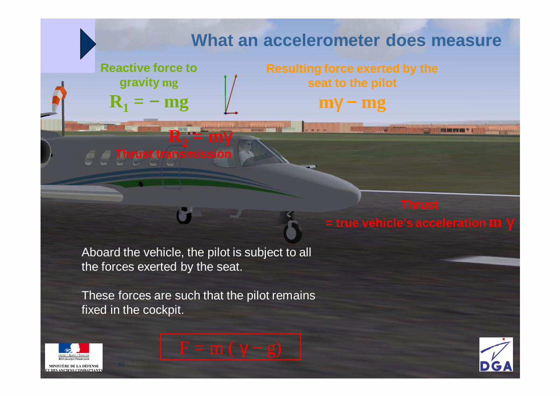
Aboard the vehicle, the pilot is subject to all the forces exerted by the seat.
These forces are such that the pilot remains fixed in the cockpit.
F = m ( γ − g)
What an accelerometer does measure
Thrust
= true vehicle’s acceleration m γγγγ
R2 = mγγγγThrust transmission
Reactive force to gravity mg
R1 = −−−− mg
Resulting force exerted by the seat to the pilot
mγ γ γ γ −−−− mg

83
An angular reference frame is necessary !
Let a vehicle turn clockwise at a constant e rotational speed ω rad.s−1
and constant tangential velocity v.
The accelerometers provide :
• Nul acceleration on the X-axis • Constant centripetal acceleration Rω2 on the Y-axis
γ γ γ γ −−−− g−−−− g
γγγγvehicle
The orientation of the measured acceleration is needed.
If the INS system assumed constant orientation, it would compute a parabolic trajectory along the Y-axis !
84
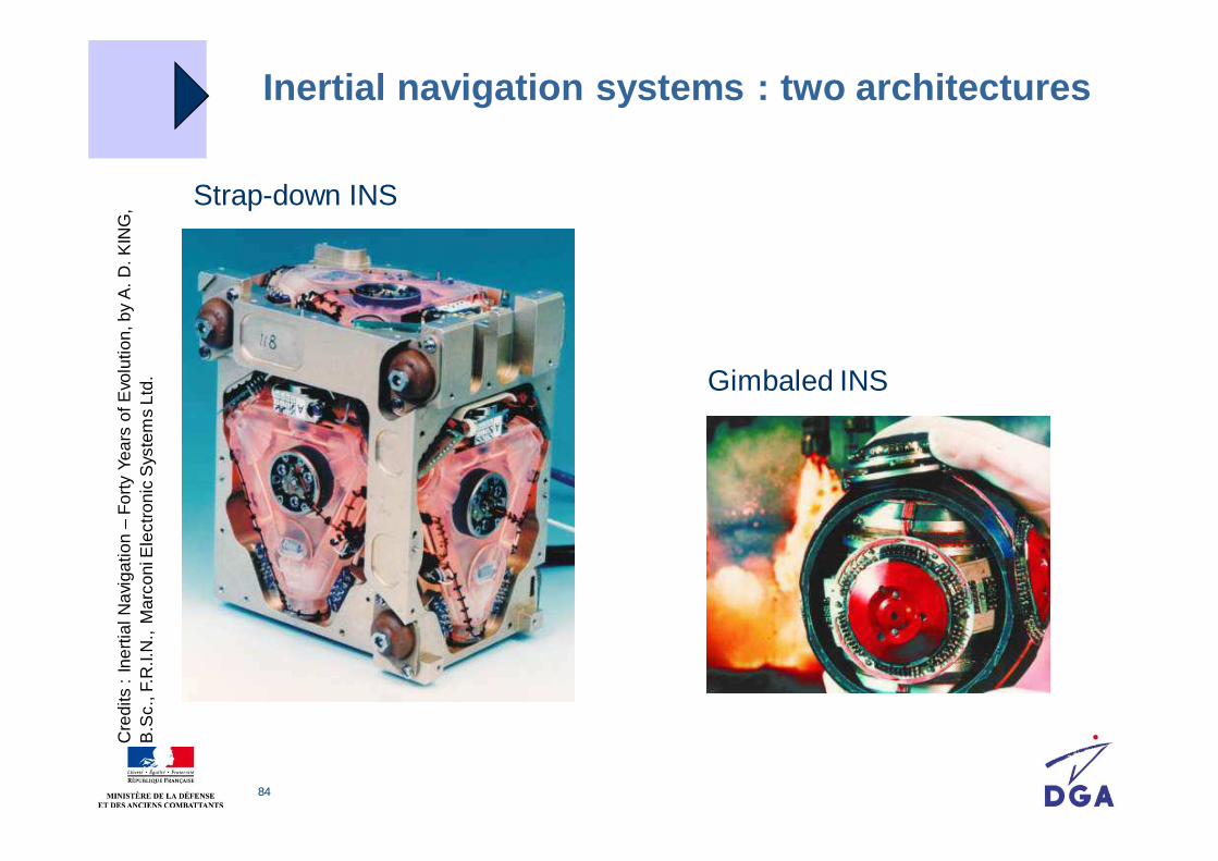
Inertial navigation systems : two architectures
Strap-down INS
Gimbaled INS
Cre
dits
:In
ertia
l Nav
igat
ion
–F
orty
Yea
rs o
f Evo
lutio
n, b
y A
. D. K
ING
, B
.Sc.
, F.R
.I.N
., M
arco
ni E
lect
roni
c S
yste
ms
Ltd.

85
Design of inertial navigation systems : two archite ctures
The angular reference is used to compensate for . Then The linear acceleration may be integrated. The position is the result of numerical integration of the speed.
The angular reference is also the reference frame, with respect to which the attitude is defined: it may then be measured or computed.
Gimbaled Strap-down
The attitude is measured on the gimbals : the reference frame is
indeed a piece of hardware.
The attitude of accelerometers is constantly integrated : the attitude of the vehicle is
computed.
gr

86
Strap-down inertial navigation systems
The inertial attitude of the accelerometer cluster is constantly integrated, so that the inertial force may be properly oriented in inertial space.
Other definitions of attitude are obtained from computations.
Elektropribor THALESTOTEM 3k

87
Gimbaled inertial navigation systems
The angular position of the vehicle is constantly mechanically compensated, so that the accelerometer platform keeps steady. Implies the use of gimbals.The vehicle attitude is measured on gimbal pickoffs, which provide the movement of the outer body around the steady platform.
Elektropribor

88
Strap-down inertial navigation systems

89
Accéléromètres et gyromètres
Accels
Gyros
axe d’entrée
fr
efrr
⋅er
Projection de l’accélération apparente sur l’axe d’entrée →
mesure
Principe de mesure : étudier et/ou rendre immobile une masse d’épreuve interne m par
rapport au boîtier
charnière
masse d’épreuve m
Impossibilité de séparer les effets de la gravité locale et des mouvements
propres du véhicule
Mesure d’une « accélération apparente » dite force spécifique
gfrrr
−= γ
axe d’entréeer
ωr err
⋅ωProjection de la vitesse de
rotation instantanée sur l’axe d’entrée → mesure Impossibilité de mesurer l’orientation
absolue du véhicule
Principe de mesure : effets Coriolis sur une masse interne m ou étude d’effets relativistes
Mesure d’une vitesse de rotation instantanée (ou débattement angulaire)

90
Strap-down inertial navigation systems
Change of coordinate frame
x
y
z
Angular integration of
gyros
x
y
z
Accels
Compensation of gravity
∫∫
Attitude of the sensor unitrelative to the reference frame
Initial attitude of the accelerometers relative to the reference frame
Initial position and velocity of the vehicle
Gyros
( ) ( ) frame refacc ffrr
→rvrr
,
rr
Vehicle attitude relative to local geodetic frame
( ) ( )( ) frame ref
frame refframe ref
g
fr
rr
+=γ
( )( ) frame refrgrr
Local gravity model
rr
Examples of reference frame : Earth Fixed Earth Centered, Copernic, …
Inertial navigation systemDouble integration of an apparent, measured acceleration • reconstructed angular position of the accel cluster, through gyros• compensated by local gravity, modeled as a function of the estimated position
Inertial navigation systemDouble integration of an apparent, measured acceleration • reconstructed angular position of the accel cluster, through gyros• compensated by local gravity, modeled as a function of the estimated position
( ) frame refγr
Angular position

91
x
y
zBody coordinate frame
x
yz
Local geodetic / navigation coordinate frame
Lon
Latxy
z
Earth Fixed Earth Centered coordinate frame
nn
bb
ee
True north pole
Common coordinate frames
tt
Inertialframe
ii
x y
z
Fixed relative to stars

92
Computation of position and velocity (1)
Velocities
So, for terrestrial applications, need to integrate :
Hence for t = EFEC :
t
rvrr ∆
= for terrestrial applications
t : EFEC or North-East-Down
for spatial vesselsi
rvrr ∆
=
( )( )rvrv
rgfr
ititit
it
ii
rrrrrrr
rrrr
×+×+×+=
+=
/// 2 ωωω
( ) ⊥Ω+×Ω−+= rvrgfv EE
t rrrrrrr 22
Time derivatives wrt rotary frames

93
Plumb bob vs Newton gravity
Earth is rotating in the inertial frame, thus inducing an inertial force that adds to the gravity field.
By the definition, we denote
And will omit the « Plumb bob » subscript in the following. Therefore :
( ) ( ) ( )rrgrgrrrrrrr ×Ω×Ω−=bob Plumb
( ) vrgfv E
e rrrrrr ×Ω−+= 2

94
Computation of position and velocity (2)
Actual computation should be able to add measured in accelerometer axes to
usually available in some global frame (eg. ECEF)
Therefore : a coordinate transform between accelerometer axes and global axes is absolutly needed !
some data is measured : modeled : computed : perfectly known :
fr
( )rgrr
gyros
measdatamoddata
data
cdata

95
Computation of position and velocity (3)
How do gyros provide proper coordinate transform between global and accelerometer axes (body) ?
They measure : in body axes.
and the transition matrix from i to b obeys
ib /ωr
( )
=
z
y
x
bib
ωωω
ω /
r
( )[ ]
ib
xy
xz
yz
ibbibib
T
TTdt
d
/
///
0
0
0
⋅
−−
−=
⋅×−=
ωωωωωω
ωr
96
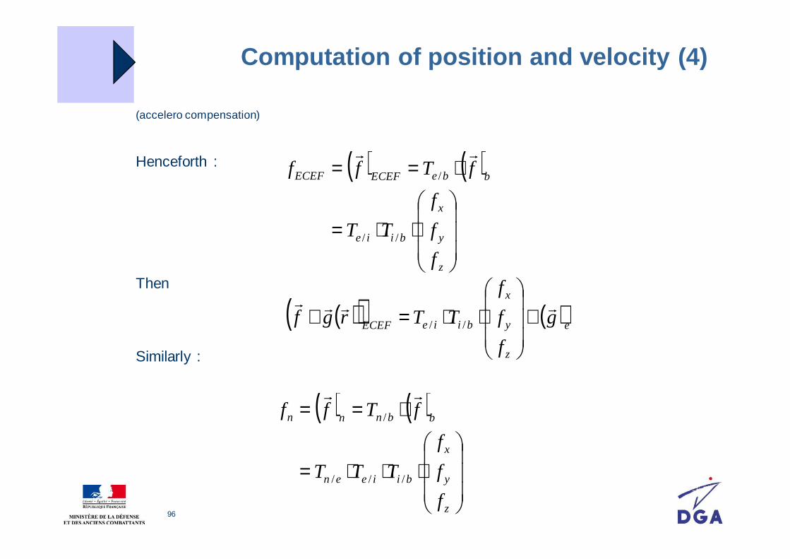
Computation of position and velocity (4)
(accelero compensation)
Henceforth :
Then
Similarly :
( ) ( )
⋅⋅=
⋅==
z
y
x
biie
bbeECEFECEF
f
f
f
TT
fTff
//
/
rr
( )( ) ( )e
z
y
x
biieECEF g
f
f
f
TTrgfrrrr
+
⋅⋅=+ //
( ) ( )
⋅⋅⋅=
⋅==
z
y
x
biieen
bbnnn
f
f
f
TTT
fTff
///
/
rr
97
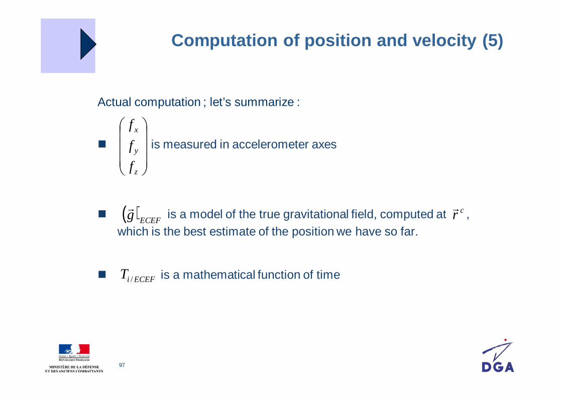
Computation of position and velocity (5)
Actual computation ; let’s summarize :
is measured in accelerometer axes
is a model of the true gravitational field, computed at , which is the best estimate of the position we have so far.
is a mathematical function of time
z
y
x
f
f
f
( )ECEFgr cr
r
ECEFiT /

98
Computation of position and velocity (6)
So the actual computation of position and velocity will involve the following in the ECEF axes :
Nota bene : need initial estimates !
( ) ( )
⋅
−−
−=
Ω+×
Ω−
+
⋅⋅=
=
⊥
cib
cib
cE
c
E
c
z
y
x
ECEFic
ibc
cc
TTdt
d
rvr
g
g
g
tTTvdt
d
vrdt
d
//
2// 0
0
2
mod
meas
0
0
0
meas
z
y
x
xy
xz
yz
ωω
ωω
ωω
f
f
f
cib
cc Tvr /,, ( ) ( ) ( )000 cb/i
cc T,v,r

99
Computation of position and velocity in n (7)
Le cas de n = Trièdre Géographique Local (TGL) ou North-East-Down
avec
( ) ( ) vrgfv E
n rrrrrrr ×Ω+−+= 2ρ
en /ωρ rr ∆=
100
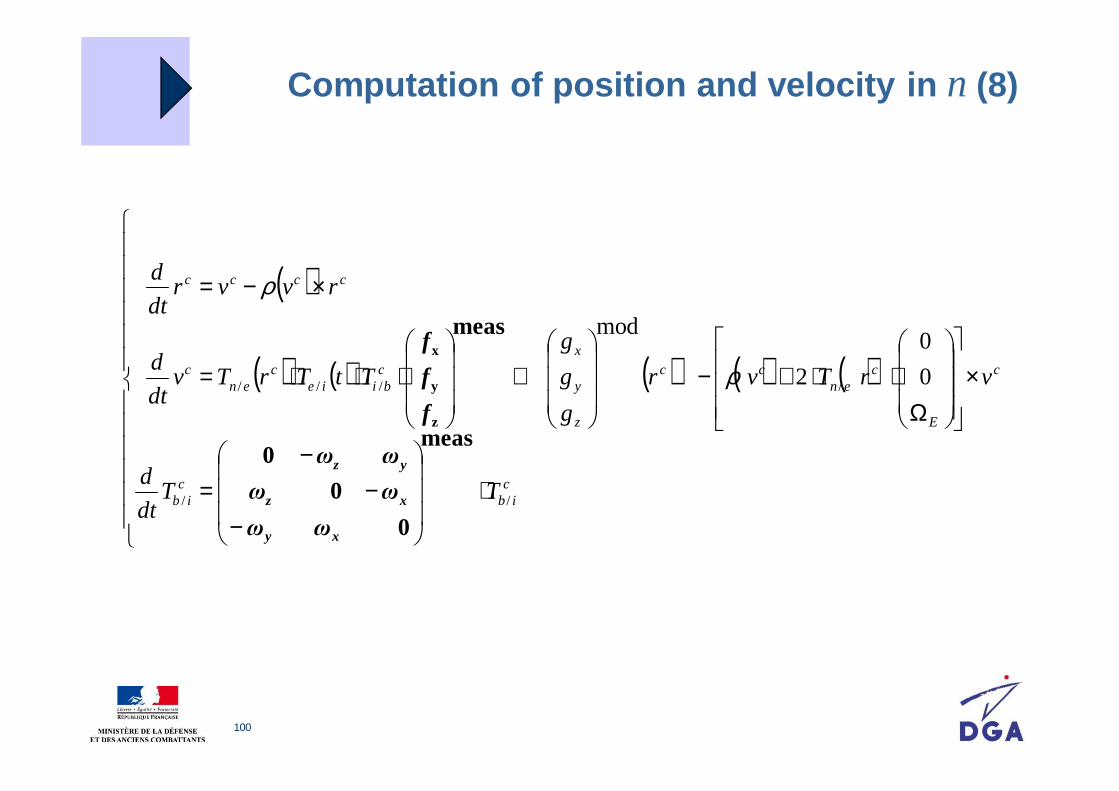
( )
( ) ( ) ( ) ( ) ( )
⋅
−−
−=
×
Ω⋅⋅+−
+
⋅⋅⋅=
×−=
cib
cib
c
E
cen
cc
z
y
xcbiie
cen
c
cccc
TTdt
d
vrTvr
g
g
g
TtTrTvdt
d
rvvrdt
d
//
//// 0
0
2
mod
meas
0
0
0
meas
z
y
x
xy
xz
yz
ωω
ωω
ωω
f
f
f
ρ
ρ
Computation of position and velocity in n (8)

101
Hardware design of computation

102
Strap-down INS : two time scales
Schematic of strap-down calculus
Sen
sor
acqu
isiti
on
Acquisition and processing of sensor data
Thermal compensations
Virtual platform Interfaceacceleros +
acceleros -
dither
gyros
velocity increments
angular increments
attitudes
quaternion
angular velocity
linear velocity
acceleros sums
temperatures
Compensation parameters
High frequency
Low frequency

103
Strap-down INS : two time scales, why ?
ConingSculling Centrifugal
accelerations
aktz −=Ω∫ π2d(Goodman theorem)
ΩΩΩΩ
Ωz
YX
Gyro input axis
Z
Sinusoidal acceleration input γ = γο cosωt
Simultaneous rotation of input axis at ωrad/s
ψ = ψ0 cos (ωt + φ)then the accelerometer X will be biased by
γγγγ
Rotational perturbation
φψγ cos2
100sculling =B
γγγγcentrifugal
L
ω=ϕ&Rotation of IMU
2centrifuge ωγ L=

104
Strap-down INS : two time scales, why ?
High frequency process
acquisition gyros
acquisition capteurs de
vitesse d’activation
filtrage d’activation
mise à l’échelle
correction mésalignements
correction mouvements
coniques
correction de bras de levier
correction de sculling
(mvt. de godille)
correction mésalignements
mise à l’échelle
acquisition accéléros +
acquisition accéléros
−correction
de non linéarité
facteurs d’échelle mésalignements
mésalignementsfacteurs d’échelle
dérives
incréments angulaires
incréments de vitesse
biais
cumuls gyros
cumuls accéléros
+
cumuls accéléros
−
+
+
+
+
+
−
−
vitesses d’activation
Acquisition
Correction
105
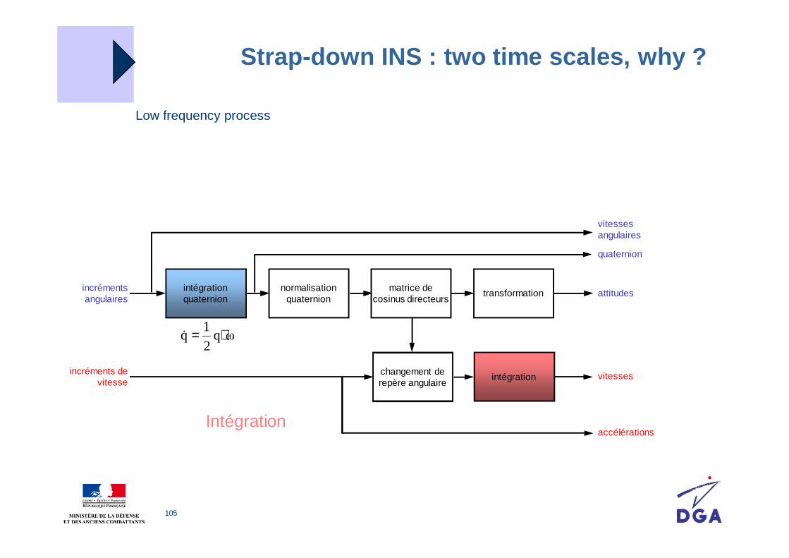
Strap-down INS : two time scales, why ?
Low frequency process
intégration quaternion
normalisation quaternion
matrice de cosinus directeurs
changement de repère angulaire
intégration
transformation
incréments de vitesse
incréments angulaires
attitudes
vitesses angulaires
quaternion
vitesses
accélérations
ωq2
1q ⋅=&
Intégration

106
Hardware design of system

107
Strap-down INS
Strap-down INS TOTEM 3000 (THALES)

108
Strap-down INS
Inertial measurement unit

109
Strap-down INS
FIN3110 instrument cluster
Marconi FIN3110 ring laser gyro inertial navigation unit
Credits : Inertial Navigation – Forty Years of Evolution, by A. D. KING, B.Sc., F.R.I.N., Marconi Electronic Systems Ltd.

110
Strap-down INS
MIMU (Space applications)
HG9900 IMU (from datasheet online)

111
Inertial Navigation SystemsKey issues

112
Key elements of inertial systems
Supporting mechanics
Inertial sensorsGyroscopes and rate gyros
AccelerometersPerformance under
environment, reliability
Stiffness, EM shielding, precision,
optical alignment
SuspensionsShock damage avoidance
Vibration isolation
Control electronicsDedicated compensations
Mechanical housingStiffness, EM shielding, precision, optical alignment, thermal draining, handling
Navigation computerOptimized and modular algorithms,
safety design objectives
Input/Output boardVersatility, performance, safety design objectives
Power supplyStability, power consumption

113
INS : thermal issues
Thermal stabilization
The performances of inertial sensors may significantly depend on temperature. Therefore it might be necessary to control the effects of thermal drifts :
control the temperature of the sensors and/or environment : needs thermal insulation materials and thermostating devicesGimbaled INS are more concerned.
correct thermal drifts using models : needs calibrationModels of order 2, 3 or 4 are used on strap-down systems, whose computation power is appropriate.

114
INS : vibratory environment issues
Suspension The main purpose is to reject vibratory perturbances due to the
environment or dithers. It might be crucial for the inertial sensors to survive the mechanical environment ! performances (coning, sculling, …)
The design of the vibration dampers is a compromise between the passband the efficiency of correction algorithms (coning, sculling) the need to activate laser gyros (dithers).
The design of a strap-down system usually requires the cancellation of assymetric effects and angular disturbances.
Popular vibration damping : pods rings

115
INS : design issues
TechnologyChallenges Gimbaled Strap-down
DesignHard & Complex
Servoing of gyrosTransmitting signals through gimbals requires slip rings
Easy…but HF computations and balancing of IMU
Manufacturing& servicing/maintenance
ComplexMany piecesResolvers
EasyVery few pieces
Calibration Easy Hard
Computation time Small Large
Range of vehicle orientationsRestricted
Gimbals may lock when reaching some positions
FullIf gyro integration algorithm appropriate (quaternion)
IntegrityIntrinsic property
of the « inertial » platformHard
fault in electronics may induce loss of all computations !

116
Inertial navigation systems : take home ideas
Discrete, independent Non-jammableAvailable, reliableUniversal coverage
Very expensiveAccuracy is also a function of volume and mass
Divergent accuracyOperational constraints

117
Structure of INS errors

118
Computation of position and velocity (recall)
The actual computation of position and velocity will involve the following in the ECEF axes :
Nota bene : need initial estimates !
( ) ( )
⋅
−−
−=
Ω+×
Ω−
+
⋅⋅=
=
⊥
cib
cib
cE
c
E
c
z
y
x
ECEFic
ibc
cc
TTdt
d
rvr
g
g
g
tTTvdt
d
vrdt
d
//
2// 0
0
2
mod
meas
0
0
0
meas
z
y
x
xy
xz
yz
ωω
ωω
ωω
f
f
f
cib
cc Tvr /,, ( ) ( ) ( )000 cb/i
cc T,v,r

119
Error analysis : coordinate transform error (1)
Coordinate transform errorsLet’s denote the (small) vector such that
We could show that satisfies the following :
where is defined in the accelerometer axes as
( )( ) ibic
ib TψT // Id ⋅×−≅ r
ψr
ψr
gyroεψ rr−=
i
gyroεψ rr−=
i
gyroεr
( ) ( ) ( )bibbibb /meas
/gyro ωωε rrr−=
« The speed of coordinate transform error as seen from the stars is exactly the gyro error. »
120
Position & Velocity errors

121
Error analysis : position and velocity errors (1)
Velocity errorLet’s denote the amount of specific force measurement error :
One can show that
accεr
( )
−
=
z
y
x
z
y
x
b
f
f
f
f
f
fmeas
accεr
( )
( ) ( ) ( )
( ) ( )⊥−⋅Ω+−×
Ω−
−+−⋅∂∂+
×
⋅+⋅=−
rrvv
rgrgrrgr
f
f
f
TTvv
cE
c
E
ECEFECEFc
ECEF
ECEF
z
y
x
ECEFbc
ECEFbc
2
modmod
/acc/
0
0
r
r&& ψε

122
Error analysis : position and velocity errors (2)
(velocity error continued)
With the assumption that , we end up with the following
« grand model » : ( ) ( )ECEFECEF rgrg ≈mod
⊥⋅Ω+⋅∂∂++×=×Ω+ rr
r
gfvv EE
t rrr
rrvrrrr δδεψδδ 2
acc2 ⊥⋅Ω+⋅∂∂++×=×Ω+ rr
r
gfvv EE
t rrr
rrvrrrr δδεψδδ 2
acc2
t here : ECEF

123
Error analysis : 3D mid-term behaviour (1)
For short to mid term applications (a few hours at most), the effects of are negligible if and are small enough.
The full model then reads :
In North-East-Down axes (NED),
EΩr
−=
⋅∂∂++×=
gyro
acc
εψ
δεψδrv
rr
rrvrr
NED
t
rr
gfv
−=
⋅∂∂++×=
gyro
acc
εψ
δεψδrv
rr
rrvrr
NED
t
rr
gfv
R
g
r
gs
s
s
s
NED
02
2
2
2
200
00
00
=
−−
≅
∂∂ ω
ωω
ωwithr
r
(spherical Earth with radius R)
rrδ v
rδ
Mid-Term Error Model (MTERM)

124
Error analysis : vertical mid-term behaviour (2)
Vertical divergenceOn the local vertical axis (D in NED), MTERM may be further developed as :
This is an exponentially unstable dynamical system, with divergence time
Consequently, when a stable navigation system is needed on the vertical axis, it may not be inertial purely !
( ) ( ) zfv sDDD δωεψδ 2acc 2++×= rvr
& ( ) ( ) zfv sDDD δωεψδ 2acc 2++×= rvr
&
s5662
1 ≅=sω
τ

125
Error analysis : horizontal mid-term behaviour (1)
Horizontal errorsOn the local horizontal plane of NED, equation MTERM now reads
( ) ( ) ( )( ) ( )
( )
−=−=
−+×+×=
DD
NENE
NEsNENEDDNENE rffv
gyro
gyro
2acc
εψεψ
δωεψψδ
r&r
r&r
rrvrvr&r( ) ( ) ( )
( ) ( )( )
−=−=
−+×+×=
DD
NENE
NEsNENEDDNENE rffv
gyro
gyro
2acc
εψεψ
δωεψψδ
r&r
r&r
rrvrvr&r

126
Horizontal errors : simplified modelWhen assuming horizontal accelerations only,
So :
The gravitational field is responsible for errors on the horizontal plane when gyros show significant horizontal reference error ( )
Significant errors due to azimut misalignment occur only if significant horizontal accelerations occur.
Error analysis : horizontal mid-term behaviour (2)
( ) ( ) ( )( ) ( )
( )
−=−=
−+×−×=
DD
NENE
NEsNENEDNENE rgv
gyro
gyro
2acc
εψεψ
δωεψψγδ
r&r
r&r
rrvrvr&r( ) ( ) ( )( ) ( )
( )
−=−=
−+×−×=
DD
NENE
NEsNENEDNENE rgv
gyro
gyro
2acc
εψεψ
δωεψψγδ
r&r
r&r
rrvrvr&r
0rr
≠NEψ
NEγrDψr

127
Error analysis : solving for horizontal errors in mi d-term (1)
Now assume constant sensor errors, as seen from the EFEC coordinate frame
Then :
and
stationary=accεrstationary=gyroεr
0 gyro, NENENE t ψεψ rrr +⋅= 0
gyro, DDD t ψεψ rrr +⋅=
in EFEC

128
Error analysis : solving for horizontal errors in mi d-term (2)
(constant sensor errors continued)
short term contributions of simply follow
short term contributions of are linear (!) :
global, mid-term oscillatory behaviour at fundamental Schüler’s frequency
NEg ψrr×−
!2
0
gyro,0
2
gyro,
apple sNewton' of speed
apple sNewton' of position
×+
×=⋅×+⋅×
NE
NENENE tgt
g
ψ
εψεr
rrrrr
accεr t⋅accεr

129
Error analysis : solving for horizontal errors in s hort-term (more graphically !)
0 2 4 6 8 10 12 14 16 18 200
1
2
3
4
5
6
7
8
9
10
Vel
ocity
err
or (
m/s
)
Time (min)
1 mg
0,1 mg
0,01 mg
10 mg
0,001 °/h
0,01 °/h
0,1 °/h
1 °/h
0 2 4 6 8 10 12 14 16 18 200
200
400
600
800
1000
1200
1400
1600
1800
2000
Time (min)
Pos
ition
err
or (
m)
0,001 °/h
0,01 °/h
0,1 °/h
1 °/h
0,01 mg
0,1 mg
1 mg
10 mg
accelerometer bias or g ×××× initial alignment error rate gyro bias

130
Error analysis : solving for horizontal errors in m id-term (more graphically !)
Mid-term Schüler damping effect
Initial position error
Rate gyro bias
Accelero bias
0
0
0
positionsvelocities
84 min

131
P & V mid-term errors : orders of magnitude
0 0.5 1 1.5 2 2.5 3-8
-6
-4
-2
0
2
4
6
8
Time in h
Vel
ocity
err
or (
m/s
)
0 0.5 1 1.5 2 2.5 3-2
-1.5
-1
-0.5
0
0.5
1
1.5x 10
4
Time in h
Pos
ition
err
or (
m)
1 mg
0.1 mg
1 mg
0.1 mg
0.1 °/h
0.01 °/h0.01 °/h
0.1 °/h
0.001 °/h 0.001 °/h
accelerometer bias or g ×××× initial alignment error rate gyro bias

132
Analytical expressions of mid-term velocity errors
It can be shown that velocity errors have a response to gyro drift as follows
Maximum errors are thus
( )( )tDR
tDR
v
v
SN
SW
W
N
ωω
δδ
cos1
cos1
Terre
Terre
−⋅⋅−⋅⋅−
==
Application: consider 0,01°/h on each input axis N, W, U⇒ 0,01×60’ /h = 0,60 ’/h = 0,60 Nm/h = 0,60 ktssince 1°= 60’ = 60 Nm on the Earth (otherwise stated: RTerre x 1° = 60 Nm)
NWMax DRv ,Terre2 ⋅⋅=δ

133
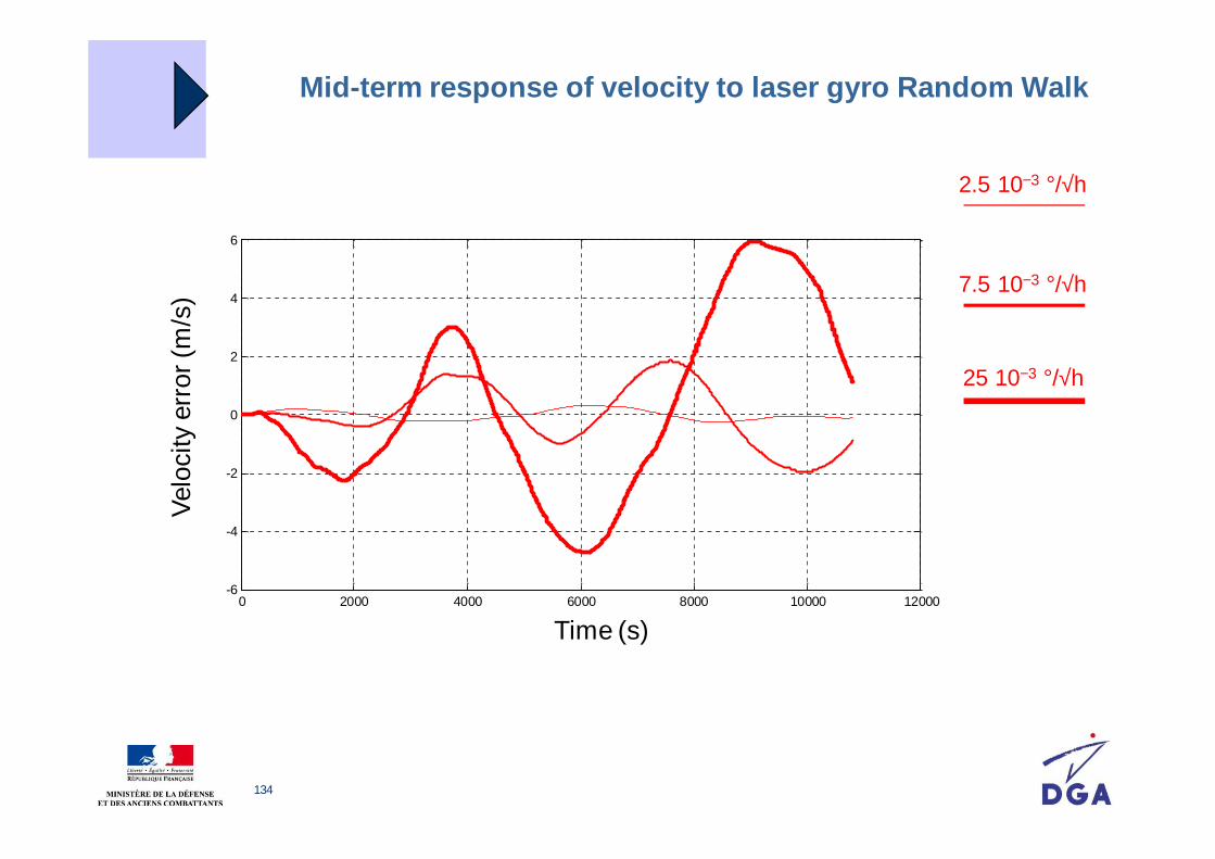
Schüler stabilizing effect
Medium term error propagation : Schüler’s term starts beeing more and more sensitiver
r
g rr
r
∆∂∂
The difference between the computedgravitational horizontal component and thetrue component has an opposite sign to thehorizontal position error.
Henceforth the horizontal Schüler componenthas a stabilizing effect on horizontal error.
Mtrue
Mcomputed
∆∆∆∆g
Mtru
e
Mcomputed
∆∆∆∆g
The difference between the computedgravitational vertical component and the truecomponent has the same sign as the verticalposition error.
Henceforth the vertical Schüler componenthas a destabilizing effect on vertical error.
g(Mcomputed )
g(Mtrue )
134
Mid-term response of velocity to laser gyro Random Walk
2.5 10−3 °/√h
7.5 10−3 °/√h
25 10−3 °/√h
Time (s)
Vel
ocity
err
or (
m/s
)
0 2000 4000 6000 8000 10000 12000-6
-4
-2
0
2
4
6

135
Altitude error
Time in min
Altitude error in m
Mean time of divergence : 9 min 30 s
Exponentially divergent altitude errors
Such a divergent nature
• precludes using of INS as a sole reference for altitude
• calls upon vertical hybridization, with GPS and/or pressure sensor
Initial errors :altitude = 10 mspeed = 0,2 m.s−1
No sensor error !

136
Attitude & Heading errors

137
Error analysis : attitude error (1)
The attitude is defined as the transition matrix from the angular reference frame to the body frame :
So for instance, when reference = NED (which is a local frame):
This leads to the actual computation of attitude :
reference/bT
NEDiib
NEDbb
TT
TT
//
/reference/
⋅==
cc NEDb
cb TT
/reference/ =
function of computed position

138
Error analysis : attitude error (2)
With the following conventional notations
one can show that
Therefore the computed attitude error reads :
( ) ×−=⇒⋅×−≅ ψψ IdId/// bbib
cib cTTT
( ) ×−=⇒⋅×−≅ θθ IdId/// NEDNEDiNED
ciNED cTTT
( ) NEDbNEDbTT cc //
Id ⋅×−≅ ϕ
ϕθψ rrv +=
ψθϕ vrr −=

139
Error analysis : attitude error (3)
The main result to keep in mind about attitude errors wrt the local geodetic frame (NED) is that horizontal components are pretty much bounded !
The divergent horizontal position errors are compensating for the inertial reference error : horizontal errors are reflecting inertial reference errors.
Horizontal components of attitude errors are damped by gravity through Schüler loops (accelerometers) : since the gravitation field is essentially vertical, the local horizontal plane is the orthogonal to accelerometers’ signals. This information is biased when the vehicle is accelerating along the horizontal plane – but it shan’t be long term.
Note : due to Earth’s rotation around the North-South axis (so-called « World axis »), is roughly spir aling around this axis : hence the equatorial components are bou nded, the world component is linearly diverging in time. This property leads to longitude divergence of horizonta l errors, that is to say North component of .
θr
ψv
ψv
θr

140
500 1000 1500 2000 2500 3000 3500 4000 4500 5000
-0.2
-0.1
0
0.1
0.2
0.3
0.4
0.5
1,0 °/h
10 °/h
0,1 °/h
10 mg
1,0 mg
0,10 mg
Mid-term vertical errors (roll & pitch)
Time in seconds
Degrees

141
Mid and long term true heading errors
0 2 4 6 8 10 12 14 16 18 20
0
5
10
15
20
25
Time in hours
1,0 °/h
10 °/h
0,1 °/h 10 mg
Degrees
142
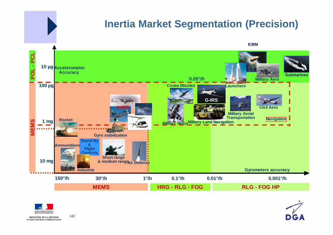
Inertia Market Segmentation (Precision)
1 mg
Gyrometers accuracy
AccelerometerAccuracy
150°/h 1°/h 0.1°/h 0.01°/h 0.001°/h
10 mg
100 µg
10 µg
Launchers
Military Aero
Military Land Navigation
30°/h
Civil Aero
Ammunitions
Short range& medium range
Military Helos
Gyro stabilization
Air Defense
AHRSMilitary Aerial
Transportation
Cruise Missiles
G-IRS
Stand-By&
Flight Controls
Rocket
Industrie
0.05°/hSubmarines
Navigation
ICBM
HRG - RLG - FOG RLG - FOG HPMEMS
ME
MS
PO
L -
PC
L

143
Hybridization

144
Hybrid technologies (inertial system/ x)
The hybridization of an inertial navigation system with a non-inertial is necessary to prevent from the vertical divergence (when mid-term navigation is a requirement). altitude sensor : GNSS, baro-altimeters, vision, … altitude blocking
The hybridization is also a mean to preclude horizontal (velocity) oscillations, using : odometers GNSS zero velocity updates (the user or some sensor raises a flag as
soon as the vehicle stops in the environment)
The most popular technique of hybridization is the Kalman filter (and brother filters)

145
Stochastic hybridization techniques (1)
Kalman filter Optimal choice when the dynamics and measurement are
linear with gaussian noise, and perfectly known If the linear dynamics and noises are not perfectly known, a
robust tuning of the filter might fit : nevertheless a robust set of parameters may provide ultra-conservative results !
Extended Kalman filter Used when dynamics and/or measurement are analytically
non-linear Poor performance if non-linearities are too strong No theoretical guarantee of optimality

146
Stochastic hybridization techniques (2)
Particle filtering Used when dynamics and/or measurement are strongly non-linear Particle = (roughly speaking) one simulation of the system at a given
initial state. Hence particle filtering makes massively parallel simulations of the real system → the particle which best explains measurements is selected probabilistically
No theoretical guarantee of optimality, unless the number of particles is infinite !
Unscented (or Sigma points) Kalman filter Used when dynamics and/or measurement are analytically non-linear Tries to inherit nice properties of particle filtering in presence of strong
non-linearities : the idea is to extend the exploration space at most, without increasing the number of particles. Hence UKF chooses deterministic values in state space to explore (so-called « Sigma points »).

147
Hybrid technologies (inertial system/ x)
Various architectures are practiced: from « loose » to « ultra-tight » « loose » = GPS position and/or velocity updates « ultra-tight » = « radio-inertial navigation system »

148
Principle of a navigation filter
1 2
p v a ω v p
−
δp0 δv0 Ψ εb εg
δp δv δa δω
Deviation
model
δp0
δv0
Ψ
εb
εgNavigation filter
1 2
INS Other equipment
p v a ωFiltered

149
Advantages and drawbacks… hybridized !
The hybridization often allows for better accuracy and/or cheaper sensors mutual calibration « in run calibration » fault detection and analysis
sensor redundancy
Be always aware ! Appropriate modeling of causality (e.g.dynamical models) is the fundamental condition to these positive effects of hybridization.
An hybridized system also inherits drawbacks of subsystems less availability dependancy on American DoD, when hybridizing GPS

150
Hybridization of INS and GPS provides better equilibri um in cost, accuracy, accuracy, dependency, vulnerability
INS and GPS : two navigation means thatcomplement each other
Discrete, independent
Non-jammable
Available, reliable, highpass
Universal coverage
Provides whole navigation data
Very accurate over the short term
Fully autonomous
Very expensive
Accuracy is a function of volume and mass
Poor, divergent accuracy over the long term
Operational constraints
Very accurate anytime
Free service very cheap function (civil)
No operational constraint in civil services
Very compact form factor
Provides position and velocity only (no angles)
Availability not compatible with high integrity reqs.
Low/no availability in certain zones
Operational constraints in military services (key management)
Noisy over the short term
Highly jammable
Dependent on the USA

151
Hybridization example : INS/GPS (2)
Specific terminology closed loop : the filter estimates are backwarded to the INS
loops (velocity for instance) tight coupling : GPS pseudo-ranges are provided by the
receiver, as updates to the hybridization filter Ultra-tight coupling : updates are INS increments and GPS
pseudo-ranges (no separate computation of velocity or position)
Inertial aid : the GPS receiver stage is provided with inertial informations
152
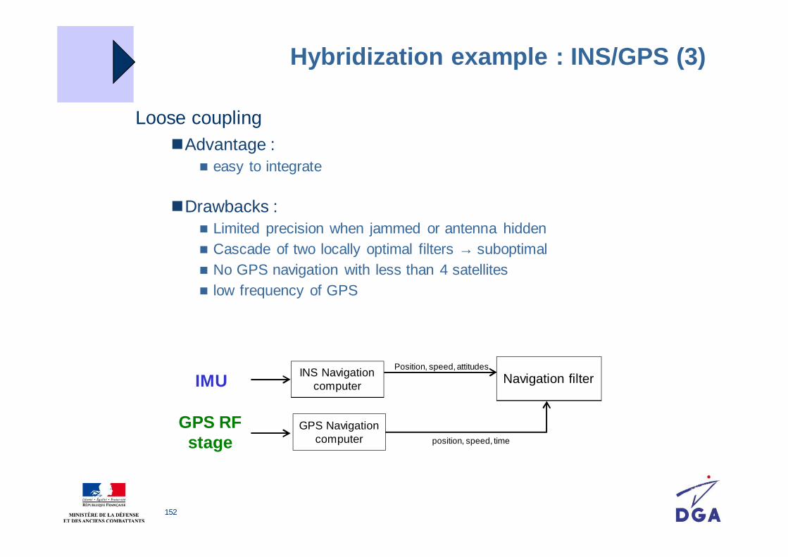
Hybridization example : INS/GPS (3)
Loose coupling Advantage :
easy to integrate
Drawbacks : Limited precision when jammed or antenna hidden Cascade of two locally optimal filters → suboptimal No GPS navigation with less than 4 satellites low frequency of GPS
Navigation filterPosition, speed, attitudes
position, speed, time
GPS Navigation computer
IMU
GPS RF stage
INS Navigation computer

153
Hybridization example : INS/GPS (4)
Loose INS / GPS with filter loopbackAdvantage :
INS errors maintained small → linear error models
Drawbacks : possible biased GPS measurements loop back to INS short term noise pollution of the INS
corrections Navigation filterPosition, speed, attitudes
GPS Navigation computer
INS Navigation computerIMU
GPS RF stage position, speed, time

154
Hybridization example : INS/GPS (5)
Tight INS / GPS coupling with INS or filter aid of GPSAdvantages :
reduced lock-on time of the GPS receiver stage more robust to jamming higher robustness against signal losses due to dynamics higher GPS frequency
Drawbacks : IMU is necessary robustness against jammers can be deceiptful
pseudo-ranges, doppleror GPS solutions
Navigation filterPosition, speed, attitudes
GPS Navigation computer
IMU
GPS RF stage
INS Navigation computer
155
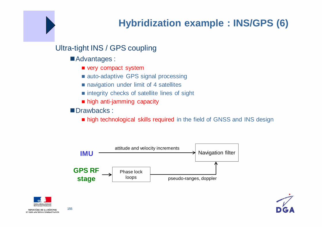
Hybridization example : INS/GPS (6)
Ultra-tight INS / GPS couplingAdvantages :
very compact system auto-adaptive GPS signal processing navigation under limit of 4 satellites integrity checks of satellite lines of sight high anti-jamming capacity
Drawbacks : high technological skills required in the field of GNSS and INS design
Navigation filterattitude and velocity increments
pseudo-ranges, dopplerPhase lock
loops
IMU
GPS RF stage

156
Appendices

157
French/English terminology
Centrale inertielle de navigation Inertial navigatio n system
Cardan Gimbal
Plate-forme à cardans Gimbaled platform
Contacts tournants Slip rings
Thermostat Thermostat
Thermostatisation Thermostating
Suspension Suspension
Suspension antivibratoire Vibration damping element
Mécanisation Mechanization
Spire Coil
Fibre optique Optical fiber
Odomètre Odometer
Centrifugeuse Centrifuge
Calage angulaire Setting angle
Panne Fault
Intégrité Fault tolerance, integrity
Guidage Guidance
Pilotage Control
Navigation Navigation
Localisation Localization
Missile balistique Ballistic missile
Spécification Requirement
Prédiction Predication phase
Recalage Update phase
Moindres carrés Least squares
Hybridation, couplage Coupling
Couplage lâche, serré, très serré (GPS) Loose, tight , ultra-tight coupling (speaking of GPS)
158
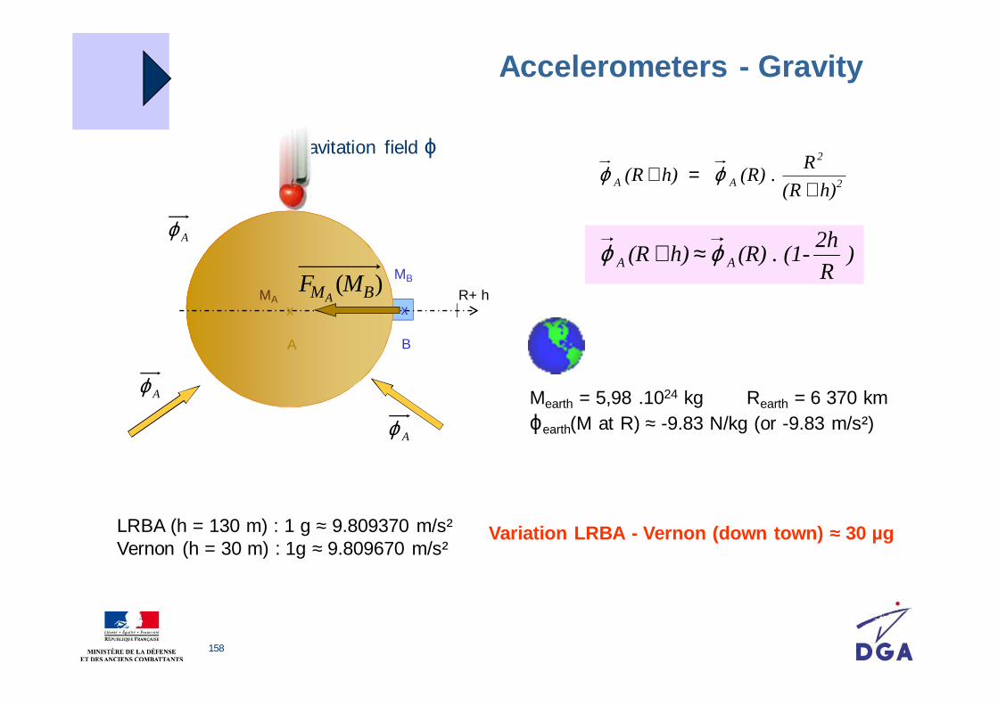
Gravitation field ϕ
MA
MB)( BM MFA
x
B
x
A
Aϕ
Aϕ
Aϕ
R+ h
2
2
AA h)(R
R(R) . h) (R
+=+ ϕϕ
Mearth = 5,98 .1024 kg Rearth = 6 370 km ϕearth(M at R) ≈ -9.83 N/kg (or -9.83 m/s²)
Variation LRBA - Vernon (down town) ≈≈≈≈ 30 µg
)R
2h(R) . (1-h)(R AA ϕϕ ≈+
LRBA (h = 130 m) : 1 g ≈ 9.809370 m/s² Vernon (h = 30 m) : 1g ≈ 9.809670 m/s²
Accelerometers - Gravity

159
Gyros : what is deg.h -1 ?
Gyro’s main performance expressed in deg.h-1
Earth rotation = 1 revolution / day = 360 deg / 24 hours~ 15 deg.h-1
Think of 1 deg.h-1 as roughly 1/15 of the earth rotation during 1 hour
Earth rotation rate
15.041 deg.h -1
EΩr

160
Sensor performance modeling
Main concepts
161
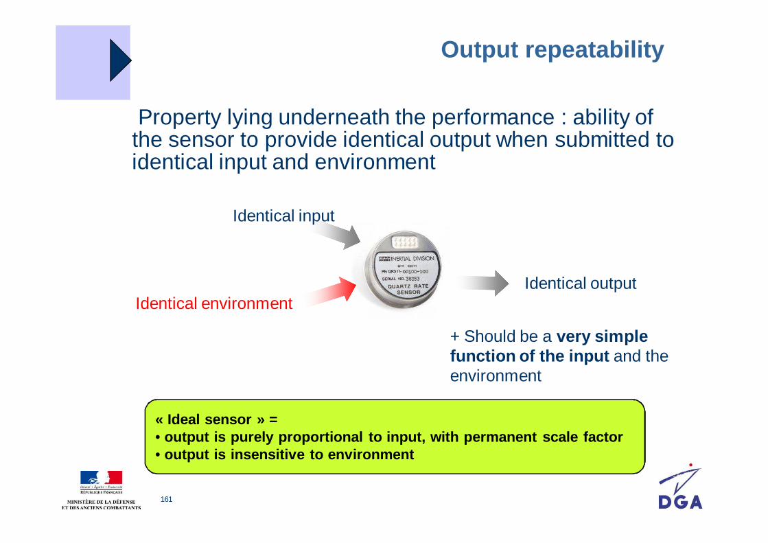
Output repeatability
Property lying underneath the performance : ability of the sensor to provide identical output when submitted to identical input and environment
Identical input
Identical environmentIdentical output
+ Should be a very simple function of the input and the environment
« Ideal sensor » =• output is purely proportional to input, with perman ent scale factor• output is insensitive to environment

162
Unitary sensor model
K1
K2
K3
K3
K2
K2+K3
Output (as)
True input
2K
3K
second order sensitivity
third order sensitivity
ε residuals
Input
•
•
•
Output
Measurements
Error / model
+⋅+⋅+⋅
∆++⋅= ε33
22
1
101 1 EKEKE
K
KKKS
E input
first order sensitivity (scale factor)1K
offset0K

163
Thermal sensitivity
Repeatability of the parameters K0, K1, K2, K3, … as functions of temperature is modeled with polynomials
-600
-400
-200
0
200
400
600
800
-50 -30 -10 10 30 50 70 90
Temperature in °C
Bias residual (µg)
-6000
-4000
-2000
0
2000
4000
6000
8000Bias variation (µg)
Bias residual (2nd order)Bias (uncompensated)
Bias = f(θ)
Uncompensated bias : 100 mm/s²/°C
(10 µg/°C)
Hysteresis
Unmodeled Biais error after compensation
(2nd order)
( )( )( )3
ref03
2ref02
ref01000
TTK
TTK
TTKKK
−⋅+
−⋅+
−⋅+=
( )( )( )3
ref13
2ref12
ref11101
TTK
TTK
TTKKK
−⋅+
−⋅+
−⋅+=
( )ref21202 TTKKK −⋅+=
( )ref31303 TTKKK −⋅+=
Offset/bias
2nd order NL
Scale factor
3rd order NL

164
Sensor mounting errors (outside of the packaging)
AX
AY
RY
RZ
RX
AZ
Accelero or gyro
AX
AY
RY
RX
2 axes - seen from above
3 axes
AXRX
Reference X-axis of the sensor cluster
Input X-axis defined on the packaging of the X-gyro/accelero-meter

165
3D sensor errors
zzyyxx efefeffrrrr
++=Measurement equation as seen from the computer,
inducing false 3D measurement : ff
rr⋅= Km
=1
1
1
K
zyzx
yzyx
xzxy
εεεεεε
fz
fr
xer
fx
fy
True measurement
yer
zer
fzm
fr
xe′r
fxm
ye′r
ze′rfy
mPerfectly aligned sensorsTheoretical
Misaligned (=real) sensors
zzyyxx efefeff ′+′+′= rrrrm
fr
mfr
zyx eeerrr
,,
zyx eee ′′′ rrr,,
False projection of the computer

166
Stability, accuracy, precision
Accuracy, stability, temporal driftEnvironment : temperature, in run, vibrations, radiations, pressure, acceleration,…

167
Vocabulary of sensor stability
« In run » stability
timeSensor off Sensor on…Short term
Self heatingPower on electrical
transients
« Run to run » stability
« Power on » / « Warm up » repeatability
Short term
Sensor output
« Warm up » time
Note : on IESI, run-to-run does not include power-on & warm-up.

168
Useful formulae
Transform of apparent velocity
Reference frame T2
1/2ωr
xxxrrrr ×−= 1/2
12
ω
( )xxxx
xxxx
xxx
rrrrrr&rr
rrrrrrr
rrrr
××−×−×−=
×−×−
×−=
×−=
1/21/2
1
1/21/2
11
1/2
1
1/2
1
1/2
1
2
1/2
122
ωωω2ω
ωωω
ω
First derivative
Second derivativehence 1/21/2
1
1/2
2
ωωω &rrr==
Reference frame T1
xr

169
Quaternions
Spectral Representation of a Rotation
αααα
When α tends to 0, the exact development simplifies to the first order as:
e : rotation axis
U
∆∆∆∆U
For any angle α,
( ) [ ] ( ) [ ]2eαcos1eαsinIαe,Rot ⋅×−+⋅×+=
( ) [ ] ( )2αeαIαe,Rot O+⋅×+=µ

170
Quaternions
Rotations vs. pass matrices
Let (a) and (b) be two orthonormal, clockwise bases.The pass-matrix from (a) to (b) is denoted Ta/b. Then the pass-matrix
from (a) to (b) is Ta/b−1 = Tb/a.
In this context, the rotation operator R=Rot(e,α) transforming (a) into (b), that is to say such that
Is represented in the base (a) by the matrix:
a/b
a
TR ≡
( ) ( )baR =
171
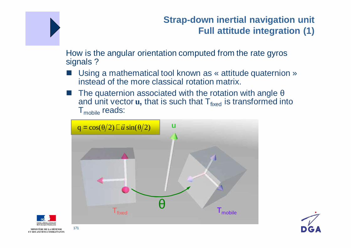
Strap-down inertial navigation unitFull attitude integration (1)
How is the angular orientation computed from the rate gyros signals ? Using a mathematical tool known as « attitude quaternion »
instead of the more classical rotation matrix. The quaternion associated with the rotation with angle θ
and unit vector u, that is such that Tfixed is transformed into Tmobile reads:
)2θsin()2θcos(q ur+=
Tfixed Tmobile
u
θ

172
Strap-down inertial navigation unitFull attitude integration (2)
Then The attitude integration in terms of quaternion space reads :
with ω : the (« quaternionized ») rotation vector from the rate gyros measurement.
This is the theoretical ordinary differential equation, that needs to be numerically integrated, using specific techniques.
ωq2
1q ⋅=&

173
Quaternions
Quaternion representationUsing the following notations,
We have :
=
=
=
=
2
αcos
2
αsine
2
αsine
2
αsine
4
33
22
11
ρ
ρ
ρ
ρ
( ) ( )( ) ( )( ) ( )
++−+−−+−+++−+−−
=24
23
22
2141324213
413224
23
22
214321
4213432124
23
22
21
a/b
22
22
22
T
ρρρρρρρρρρρρρρρρρρρρρρρρρρρρρρρρρρρρ

174
Quaternions
Quaternions’ algebra HSet of real linear combinations of 1, i, j and k, where
Isomorphism between H and the direct rotation groupWith Ta/b written as the previous slide, we uniquely associate
denoting
kkjjii
jikkiikjjkkjiij
kji
−=−=−==−==−==−=
−===
∗∗ *
222 1
2
αsin
2
αcos
4321a/b
u
kjiQ
+=
+++= ρρρρ
321 eee kjiu ++=
175
Quaternions
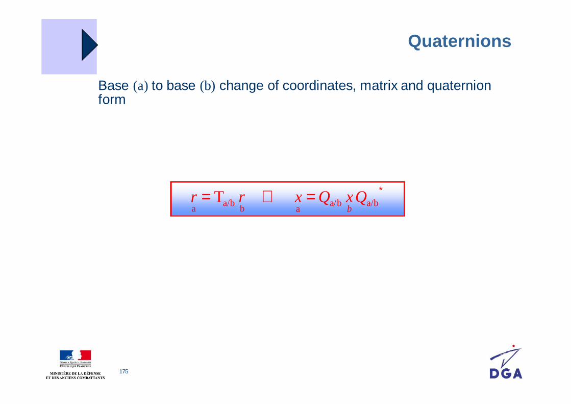
Base (a) to base (b) change of coordinates, matrix and quaternion form
∗=⇔= a/ba/bab
a/ba
T QxQxrrb
176
Quaternions
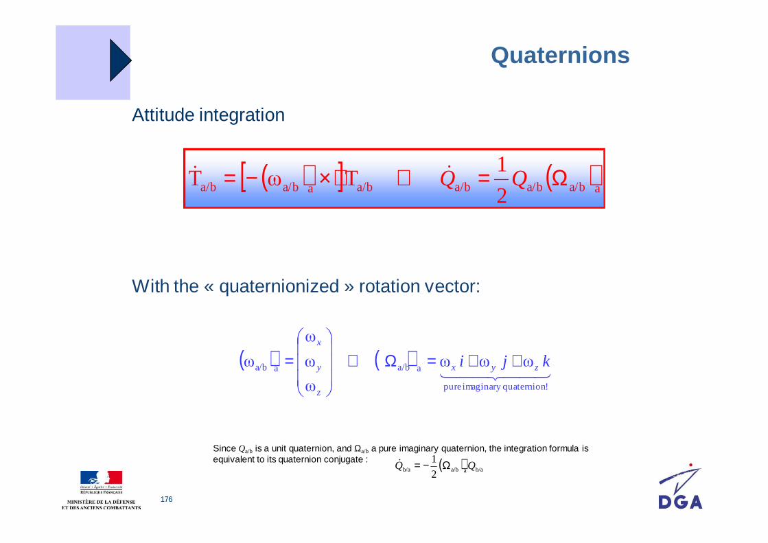
Attitude integration
With the « quaternionized » rotation vector:
( )[ ] ( )aa/ba/ba/ba/baa/ba/b 2
1TωT Ω=⇔⋅×−= QQ&&
( ) ( )44 344 21
! quaternionimaginary pure
aa/baa/b ωωω
ω
ω
ω
ω kji zyx
z
y
x
++=Ω⇔
=
( ) b/aaa/bb/a2
1QQ Ω−=&
Since Qa/b is a unit quaternion, and Ωa/b a pure imaginary quaternion, the integration formula is equivalent to its quaternion conjugate :
177
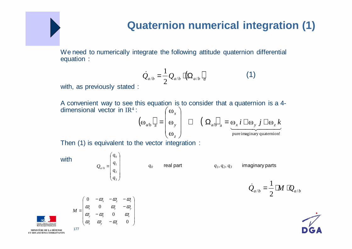
Quaternion numerical integration (1)
We need to numerically integrate the following attitude quaternion differentialequation :
with, as previously stated :
A convenient way to see this equation is to consider that a quaternion is a 4-dimensional vector in IR4 :
Then (1) is equivalent to the vector integration :
with
( )abababa QQ /// 2
1 Ω⋅=&
( ) ( )44 344 21
! quaternionimaginary pure
aa/baa/b ωωω
ω
ω
ω
ω kji zyx
z
y
x
++=Ω⇔
=
=
3
2
1
0
/
q
q
q
q
Q ba
(1)
baba QMQ // 2
1 ⋅⋅=&
−−
−−−−
=
0
0
0
0
xyz
xzy
yzx
zyx
M
ωωωωωωωωωωωω
q0 q1, q2, q3real part imaginary parts

178
We can solve this last equation between tk−1 and tk as:
provided that the vector is constant between tk-1 and tk
When the time step is small enough, angular increments are verysmall, and so is the argument of the exp. Then:
BTW, note that
Quaternion numerical integration (2)
∫∫−−
+≈
k
k
k
k
t
t
t
tMM
11 2
1Id
2
1exp 4
−−
−−−−
== ∫−
0
0
0
0
1
xyz
xzy
yzx
zyx
t
t
k
k
MA
αααααααααααα
∫−
= k
k
t
t zyxzyx1
,,,, ωαwhere are the (debiased) angular increments
( ) ( )1//12
1exp −⋅
= ∫−
kba
t
tkba tQMtQk
k
[ ]
×−
=
−−
−−−−
=.
0
0
0
0
0
ααα
αααααααααααα
T
xyz
xzy
yzx
zyx
A where
=
z
y
x
ααα
α
ba /ωr

179
Quaternion numerical integration (3)
Typical numerical schemes in practice, more accurate approximations of the previous
discrete equation may be derived a popular one :
Check [Titterton] pages 319-324 for more details
4444 34444 2144 344 21scorrection
112
2
npropagatio
11 6
1
8
1
2
1
⋅+⋅⋅−⋅+= −−−− kkkkk QAQQAQQ α
where
23
22
21
2
2vvvv ++=
[ ]
×−
=
−−
−−−−
=.
0
0
0
0
0
ααα
αααααααααααα
T
xyz
xzy
yzx
zyx
A
∫−
= k
k
t
t zyxzyx1
,,,, ωα are the (debiased) angular increments
( ) ( )1/1/ −− == kbakkbak tQQtQQ

180
Wilcox integration of quaternion
Second order
Third order
Forth order
⋅+⋅⋅−⋅+= −−−− 11
2
11 61
81
21
kkkkk QAQQAQQ α
⋅+⋅⋅+
⋅+⋅⋅−⋅+= −−−−−− 11
4
11
2
11 101
3841
61
81
21
kkkkkkk QAQQAQQAQQ αα
1
2
11 81
21
−−− ⋅⋅−⋅+= kkkk QQAQQ α

181
Strategies to reduce computation load whenunder coning motion
Any of the previous numerical schemes can lead to apparent drift errors (when coning motion exists) : finite angular resolution of the RLG superactivation high frequency vibrations vs frequency of digitial computation digital signal processing stages inside the angular integration
loop
When integrated at very high frequency.Classes of numerical schemes (Miller, Bortz) are intended to allow (rather) low frequency computation while combining high frequency « correction » terms, to circumvent virtual drifts.
182
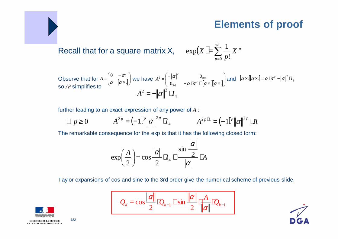
Elements of proof
Recall that for a square matrix X,
Observe that for we have andso A² simplifies to
further leading to an exact expression of any power of A :
The remarkable consequence for the exp is that it has the following closed form:
Taylor expansions of cos and sine to the 3rd order give the numerical scheme of previous slide.
[ ]
×−
=.
0
ααα T
A
( ) ∑+∞
==
0 !
1exp
p
pXp
X
[ ][ ]
××+⋅−−=
×
×
..0
0
13
31
22
ααααα
TA [ ][ ] 3
2.. IT ⋅−⋅=×× ααααα
4
22 IA ⋅−= α
( ) 4
22 1 IAppp ⋅−= α ( ) AA
ppp ⋅−=+ 212 1 α0≥∀ p
AIA ⋅+⋅=
α
αα 2
sin
2cos
2exp 4
11 2sin
2cos −− ⋅⋅+⋅= kkk Q
AQQ
ααα