1

Online Student Guide

OpusWorks 2019, All Rights Reserved

Introduction to Process Capability

2

Table of Contents

LEARNING OBJECTIVES ....................................................................................................................................4

INTRODUCTION ..................................................................................................................................................4 PROCESS CAPABILITY .................................................................................................................................................................... 4 CONTROL CHART ............................................................................................................................................................................ 4 SPECIFICATION LIMITS ................................................................................................................................................................. 5 CHARACTERISTICS OF THE DATA................................................................................................................................................ 5 POPULATION AND SAMPLES ........................................................................................................................................................ 6 SAMPLE............................................................................................................................................................................................. 6 POPULATION ................................................................................................................................................................................... 7 SYMBOLS: CENTER ......................................................................................................................................................................... 7 SYMBOLS: SPREAD ......................................................................................................................................................................... 8 SYMBOLS .......................................................................................................................................................................................... 8 SAMPLING DONE PROPERLY ........................................................................................................................................................ 9

HISTOGRAM .........................................................................................................................................................9 RELATIVE CAPABILITY .................................................................................................................................................................. 9

ASSESSING CAPABILITY ................................................................................................................................ 10

TWO TYPES OF DATA .................................................................................................................................... 11 CONTINUOUS DATA REVIEW .................................................................................................................................................... 11 DISCRETE DATA REVIEW .......................................................................................................................................................... 11

CONTINUOUS DATA ........................................................................................................................................ 12 DATA AND CUSTOMER REQUIREMENTS ................................................................................................................................ 12 DPMO AND SIX SIGMA QUALITY LEVEL ................................................................................................................................ 12 STEPS TO ASSESS PROCESS CAPABILITY ................................................................................................................................ 12 STEP 1............................................................................................................................................................................................ 13 STEP 2............................................................................................................................................................................................ 13 STEP 3............................................................................................................................................................................................ 14 STEP 4............................................................................................................................................................................................ 14 STEP 5............................................................................................................................................................................................ 15 ASSESSING DATA ......................................................................................................................................................................... 15

DISCRETE DATA .............................................................................................................................................. 15 DEFINE THE OPPORTUNITY ...................................................................................................................................................... 16 WHAT IS A DEFECT? ................................................................................................................................................................... 16 CALCULATING THE DEFECT RATE ........................................................................................................................................... 16 ESTIMATING SIGMA LEVEL ....................................................................................................................................................... 17 SIGMA LEVEL EXAMPLE ............................................................................................................................................................. 17 DISCRETE DATA .......................................................................................................................................................................... 18 IMPROVEMENT ............................................................................................................................................................................. 19

3

© 2019 by OpusWorks. All rights reserved. August, 2019 Terms of Use This guide can only be used by those with a paid license to the corresponding course in the e-Learning curriculum produced and distributed by OpusWorks. No part of this Student Guide may be altered, reproduced, stored, or transmitted in any form by any means without the prior written permission of OpusWorks. Trademarks All terms mentioned in this guide that are known to be trademarks or service marks have been appropriately capitalized. Comments Please address any questions or comments to your distributor or to OpusWorks at info@OpusWorks.com.

4

Learning Objectives

Upon completion of this course, student will be able to: • Learn that a measure of process capability can help you determine how well a process is able to

meet customer requirements • Discuss how to identify when one process is more capable than another • Distinguish capable from non-capable processes • Identify how sample measurements are used to estimate population values • Determine which Control Chart type is most appropriate for monitoring a particular process

parameter

Introduction

Process Capability

Process capability is defined as the extent to which a stable process is able to meet specifications. Embedded in this definition there are two key concepts. See if you can identify them by clicking on words that describe the concepts.

Control Chart

A control chart is a tool used to determine if a process is stable over time and is used to identify if any special causes of variation are present. When special causes of variation are present in a process, the estimates of process capability may not be reliable. The estimates computed at different time periods may be quite different. Estimates computed during the time when the process is unstable should not be used to predict how the process will behave in the future.

When the process is stable, the estimates taken at different times will be both reliable and valid. Statistical methods can be used to predict how well the process will behave in the future. Control charts are used to determine if a process is stable over time.

5

Specification Limits

The voice of your customers is represented by the specification limits. The specification limits define the customer’s requirements. You determine how well you are responding to the needs of your customers by comparing your process data, in the form of a histogram, to the specification limits.

Process capability metrics will use the voice of the process, data, to indicate how well you are listening to the voice of the customer, specification limits.

Characteristics of the Data

Three characteristics of the data that are most important when assessing capability are Shape, Center, and Spread. Let’s begin with the characteristic of shape.

6

Population and Samples

To measure the capability of a process, you will need to collect data from the process. Most often, this data will be collected by taking samples. By taking samples and plotting a histogram we often see a shape emerge that looks like this. We can use this curve to represent the population. The population represents the entire collection of process measurements. Now we can see how well the population fits within the spec limits. Let’s begin by further exploring the relationship between samples and populations.

Sample

Let’s use chocolates to illustrate some important points about population and samples. Suppose you are a Quality Inspector and you need to make sure that every chocolate covered cherry really had a cherry inside. One way to do this would be to check every one. But a far better way would be to sample. If you sample you would not have to check every piece. Besides, in this case sampling is more efficient and less costly. Testing them all would not be very smart because then you would have nothing left to sell. In this Lesson, you will see how taking samples from a process, can help you understand what the whole process is doing. But first, let’s define a very important term: Population.

7

Population

A population is all possible outputs of a process. It consists of all individual values you want to draw conclusions about. A population can be defined in many ways, depending on what you’re interested in studying. For example, if you’re trying to assure that this shipment has all the cherries it’s supposed to have, our population is all of the chocolate covered cherries in these boxes. A sample is a subset of the population. This operator is taking samples from this population of chocolates. Every chocolate in the sample is part of the population, but notice that not every chocolate is part of the sample, but they are part of the population.

Symbols: Center

Since we rarely measure the entire population, we seldom know the exact value of the center and spread. So, we use our sample data to estimate them. Let’s start with center. Two measures of center are X-bar and mu. X-bar is sample average. mu is the population average.

8

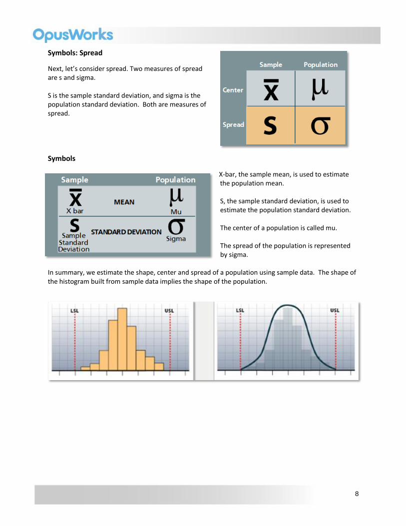
Symbols: Spread

Next, let’s consider spread. Two measures of spread are s and sigma. S is the sample standard deviation, and sigma is the population standard deviation. Both are measures of spread.

Symbols

X-bar, the sample mean, is used to estimate the population mean. S, the sample standard deviation, is used to estimate the population standard deviation. The center of a population is called mu. The spread of the population is represented by sigma.

In summary, we estimate the shape, center and spread of a population using sample data. The shape of the histogram built from sample data implies the shape of the population.

9

Sampling Done Properly

When done properly, sampling is very powerful. It saves time, makes better use of personnel, and it’s cost effective.

Histogram

With a histogram, you can look at how individual values compare to specs. By taking samples and plotting a histogram you often see a shape emerge that looks like this. You can use this curve to represent the population. Now you can see how well the population fits within the spec limits. Remember what process capability is?

Process Capability is the extent to which a stable process is able to meet specs.

Relative Capability

When our data looks like this, we can use this curve for many purposes. We can: -Compare the capability of two computer systems doing the same function, same process. -Compare the capability of two different departments or teams that perform the same process, -Or compare the capability of the same process before and after improvements. Reducing process variation is a key element of a process improvement philosophy. Process capability assessments help to track this progress.

In the following exercise you’ll have an opportunity to compare the capability of several processes. Both of these processes have the same spec limits and are centered on target.

10

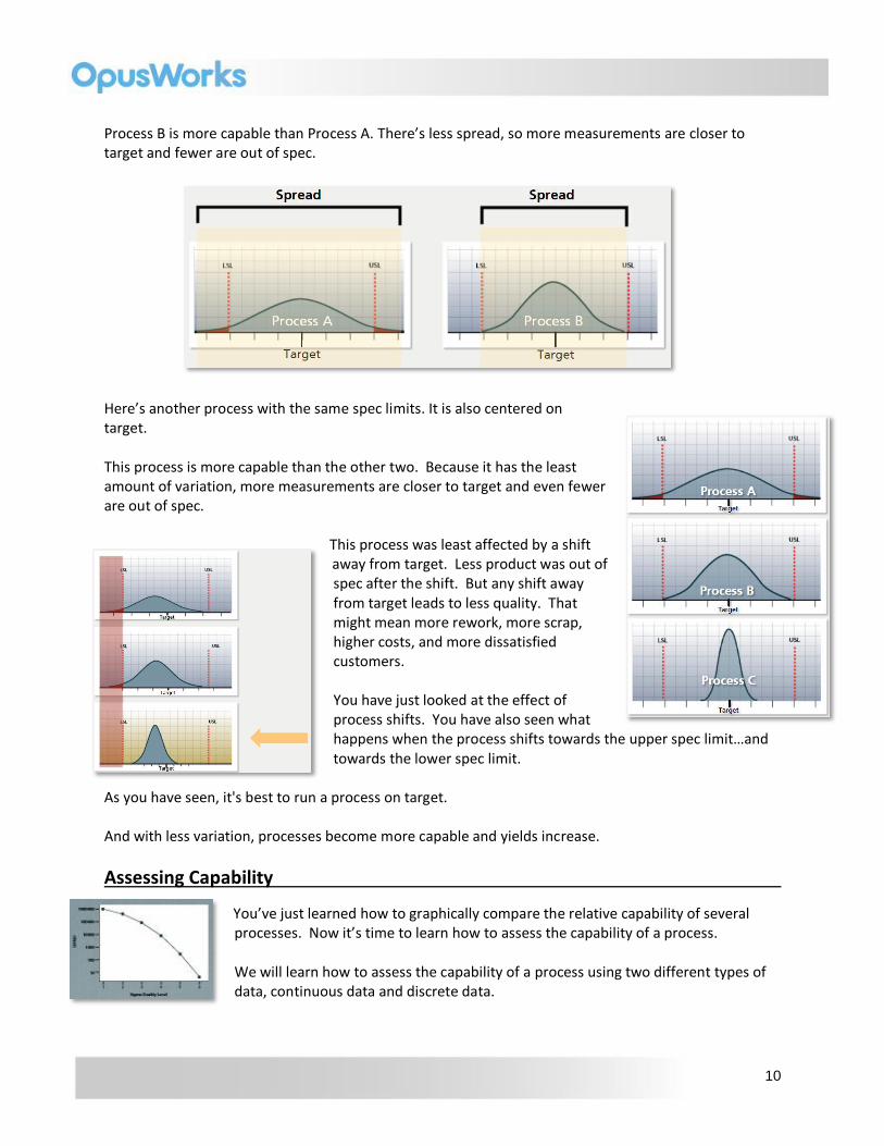
Process B is more capable than Process A. There’s less spread, so more measurements are closer to target and fewer are out of spec.

Here’s another process with the same spec limits. It is also centered on target. This process is more capable than the other two. Because it has the least amount of variation, more measurements are closer to target and even fewer are out of spec.

This process was least affected by a shift away from target. Less product was out of spec after the shift. But any shift away from target leads to less quality. That might mean more rework, more scrap, higher costs, and more dissatisfied customers. You have just looked at the effect of process shifts. You have also seen what happens when the process shifts towards the upper spec limit…and towards the lower spec limit.

As you have seen, it's best to run a process on target. And with less variation, processes become more capable and yields increase.

Assessing Capability

You’ve just learned how to graphically compare the relative capability of several processes. Now it’s time to learn how to assess the capability of a process. We will learn how to assess the capability of a process using two different types of data, continuous data and discrete data.

11

Two Types of Data

Data comes in two basic flavors; Continuous and Discrete.

Continuous Data Review

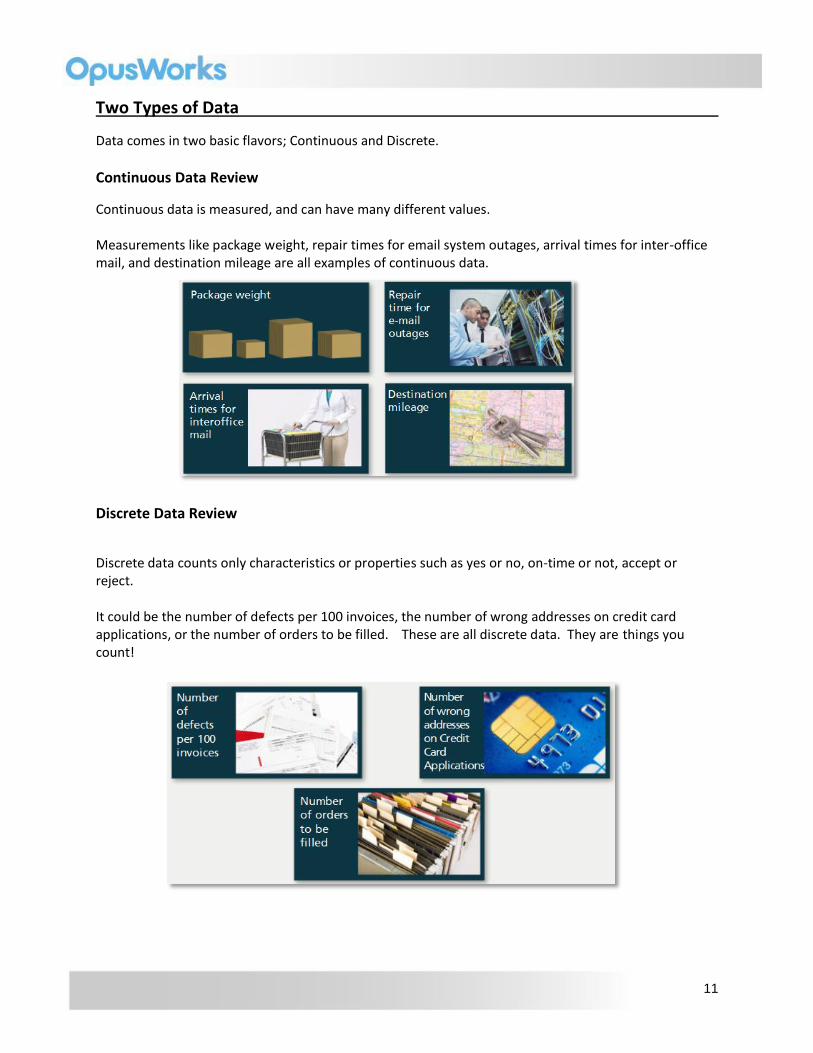
Continuous data is measured, and can have many different values. Measurements like package weight, repair times for email system outages, arrival times for inter-office mail, and destination mileage are all examples of continuous data.

Discrete Data Review

Discrete data counts only characteristics or properties such as yes or no, on-time or not, accept or reject. It could be the number of defects per 100 invoices, the number of wrong addresses on credit card applications, or the number of orders to be filled. These are all discrete data. They are things you count!

12

Continuous Data

Data and Customer Requirements

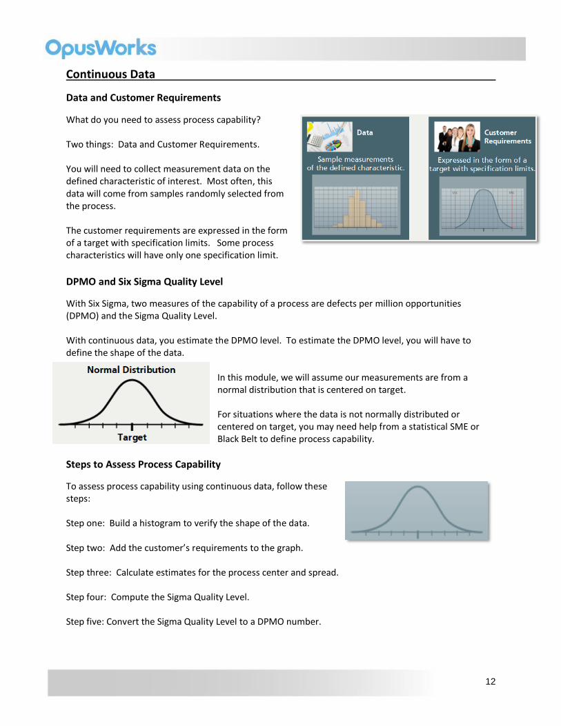
What do you need to assess process capability? Two things: Data and Customer Requirements. You will need to collect measurement data on the defined characteristic of interest. Most often, this data will come from samples randomly selected from the process. The customer requirements are expressed in the form of a target with specification limits. Some process characteristics will have only one specification limit.

DPMO and Six Sigma Quality Level

With Six Sigma, two measures of the capability of a process are defects per million opportunities (DPMO) and the Sigma Quality Level. With continuous data, you estimate the DPMO level. To estimate the DPMO level, you will have to define the shape of the data.

In this module, we will assume our measurements are from a normal distribution that is centered on target. For situations where the data is not normally distributed or centered on target, you may need help from a statistical SME or Black Belt to define process capability.

Steps to Assess Process Capability

To assess process capability using continuous data, follow these steps: Step one: Build a histogram to verify the shape of the data. Step two: Add the customer’s requirements to the graph. Step three: Calculate estimates for the process center and spread. Step four: Compute the Sigma Quality Level. Step five: Convert the Sigma Quality Level to a DPMO number.

13

Step 1

Step 1. Using sample data, build a histogram. The shape of the histogram will give you an indication if the data is normally distributed. There are statistical tests that can be used to verify if the data comes from a normal distribution. These tests are covered in a more advanced module.

Step 2

Add the customer’s requirements in the form of the specification limits and target value to the graph representing the process data. Visually, you now have a picture of the capability of the process.

14

Step 3

From the sample data, use the sample statistics X-bar as an estimate of the process mean, mu. Calculate the sample standard deviation, s and use this as an estimate of the population standard deviation, sigma.

Step 4

The Sigma Quality Level can be computed by finding the number of standard deviations that will fit between the process mean and the closest specification limit. In this example, we have one sigma, two sigma, three sigma. This is a three sigma process.

15

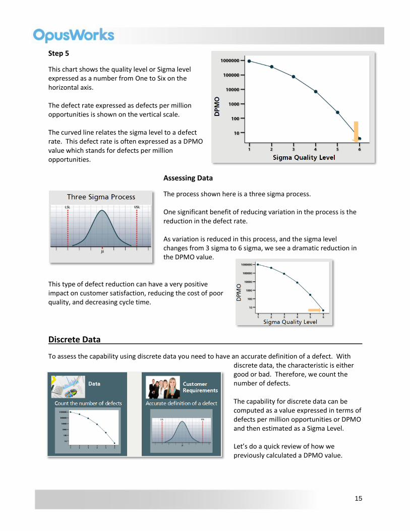
Step 5

This chart shows the quality level or Sigma level expressed as a number from One to Six on the horizontal axis. The defect rate expressed as defects per million opportunities is shown on the vertical scale. The curved line relates the sigma level to a defect rate. This defect rate is often expressed as a DPMO value which stands for defects per million opportunities.

Assessing Data

The process shown here is a three sigma process. One significant benefit of reducing variation in the process is the reduction in the defect rate. As variation is reduced in this process, and the sigma level changes from 3 sigma to 6 sigma, we see a dramatic reduction in the DPMO value.

This type of defect reduction can have a very positive impact on customer satisfaction, reducing the cost of poor quality, and decreasing cycle time.

Discrete Data

To assess the capability using discrete data you need to have an accurate definition of a defect. With discrete data, the characteristic is either good or bad. Therefore, we count the number of defects. The capability for discrete data can be computed as a value expressed in terms of defects per million opportunities or DPMO and then estimated as a Sigma Level. Let’s do a quick review of how we previously calculated a DPMO value.

16

Define the Opportunity

First we define the opportunity. An opportunity can be defined in many ways. Here we have a customer application form for a credit card. The form contains five sections. We could define the opportunity in many ways. We have decided to count each form as an opportunity and measure the defect rate at the form level.

What is a Defect?

Next we must define what is a defect. Be very specific and clear in your definition. Also, make sure everyone on your team agrees to the definition and commits to following the rules when tracking defects. In this example, we define the form as containing a defect if at least one error occurs on the form.

Calculating the Defect Rate

To calculate the defect rate as a DPMO value, we divide the number of defects by the number of opportunities and multiply by 1,000,000. In our example, 2000 were inspected and 220 were found to have defects. 220 divided by 2000 times 1,000,000 equals a DPMO value of 110,000. That means that for every 1,000,000 application forms processed, 110,000 will contain defects.

17

This is the capability of the process expressed as a DPMO value.

Estimating Sigma Level

With discrete data we compute the defect level and estimate the sigma level. This chart shows the quality level or Sigma level expressed as a number from One to Six on the horizontal axis. The defect rate expressed as defects per million opportunities is shown on the vertical scale. The values on this chart (allowing for a slight shift in the process mean) represent the long-term quality level you can expect from a process running at a stated sigma level.

Sigma Level Example

In the previous example, the DPMO value was 110,000. To convert this to a Sigma Level, we would locate 110,000 on the vertical axis. Then draw a horizontal line until it intersects the curve. At the point of intersection, we would draw a vertical line to the horizontal axis and read the Sigma Level corresponding to a DPMO value of 110,000. The Sigma Level for this process is approximately 2.73.

18

Discrete Data

Here’s a comparison of the two processes showing their DPMO and Sigma Quality Levels. With this data and the relationship between DPMO and sigma shown on this chart, it’s fairly easy to see that as the defect rate decreases, sigma will increase. A 4.38 sigma is better than a 2.73 sigma, and 6 sigma – well, that’s almost perfect quality!

3 vs. 6 Sigma Capability You have now seen how to assess the capability of a process using continuous data and using discrete data. Using the sigma quality level metric we can now use a language that is easily understood in describing and measuring our improvement efforts. As we reduce variation and improve capability, we will see a reduction in DPMO and an increase in the sigma level.

19

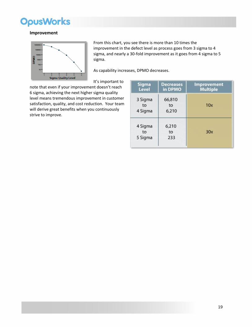
Improvement

From this chart, you see there is more than 10 times the improvement in the defect level as process goes from 3 sigma to 4 sigma, and nearly a 30-fold improvement as it goes from 4 sigma to 5 sigma. As capability increases, DPMO decreases. It’s important to

note that even if your improvement doesn’t reach 6 sigma, achieving the next higher sigma quality level means tremendous improvement in customer satisfaction, quality, and cost reduction. Your team will derive great benefits when you continuously strive to improve.