jamming ii: edwards’ statistical mechanics of random
TRANSCRIPT

Physica A 390 (2011) 427–455
Contents lists available at ScienceDirect
Physica A
journal homepage: www.elsevier.com/locate/physa
Jamming II: Edwards’ statistical mechanics of random packings ofhard spheresPing Wang, Chaoming Song, Yuliang Jin, Hernán A. Makse ∗
Levich Institute and Physics Department, City College of New York, New York, NY 10031, United States
a r t i c l e i n f o
Article history:Received 19 April 2010Received in revised form 8 September 2010Available online 20 October 2010
Keywords:Jammed matterPhase diagramVoronoi volumes
a b s t r a c t
The problem of finding the most efficient way to pack spheres has an illustrious history,dating back to the crystalline arrays conjectured by Kepler and the random geometriesexplored by Bernal in the 1960s. This problem finds applications spanning from themathematician’s pencil, the processing of granular materials, the jamming and glasstransitions, all the way to fruit packing in every grocery. There are presently numerousexperiments showing that the loosest way to pack spheres gives a density of∼55% (namedrandom loose packing, RLP) while filling all the loose voids results in a maximum densityof ∼63%–64% (named random close packing, RCP). While those values seem robustly true,to this date there is no well-accepted physical explanation or theoretical prediction forthem. Here we develop a common framework for understanding the random packingsof monodisperse hard spheres whose limits can be interpreted as the experimentallyobservedRLP andRCP. The reason for these limits arises froma statistical picture of jammedstates in which the RCP can be interpreted as the ground state of the ensemble of jammedmatter with zero compactivity, while the RLP arises in the infinite compactivity limit.We combine an extended statistical mechanics approach ‘a la Edwards’ (where the roletraditionally played by the energy and temperature in thermal systems is substituted bythe volume and compactivity) with a constraint on mechanical stability imposed by theisostatic condition. We show how such approaches can bring results that can be comparedto experiments and allow for an exploitation of the statistical mechanics framework. Thekey result is the use of a relation between the local Voronoi volumes of the constituentgrains (denoted the volume function) and the number of neighbors in contact that permitsus to simply combine the two approaches to develop a theory of volume fluctuations injammed matter. Ultimately, our results lead to a phase diagram that provides a unifyingview of the disordered hard sphere packing problem and further sheds light on a diversespectrum of data, including the RLP state. Theoretical results are well reproduced bynumerical simulations that confirm the essential role played by friction in determiningboth the RLP and RCP limits. The RLP values depend on friction, explaining why variedexperimental results can be obtained.
© 2010 Elsevier B.V. All rights reserved.
1. Introduction
Filling containerswith balls is one of the oldestmathematical puzzles known to scientists. The study of disordered spherepackings raises an interesting problem: how efficient and uniform will spheres pack if assembled randomly? This problemhas an important application in the jamming phenomenon, which takes place in particulate systems where all particles are
∗ Corresponding author.E-mail address: [email protected] (H.A. Makse).
0378-4371/$ – see front matter© 2010 Elsevier B.V. All rights reserved.doi:10.1016/j.physa.2010.10.017

428 P. Wang et al. / Physica A 390 (2011) 427–455
in close contact with one another. The study of jammed granular media offers unexpected challenges in physics since theequilibrium statistical mechanics fails for these out-of-equilibrium systems. The goal of the present study is to develop anensemble theory of volume fluctuations to describe the statistical mechanics of jammed matter with the aim of sheddinglight on the long-standing problem of characterizing random sphere packings.
1.1. Sphere packing problem
The study of the sphere packing problem started four centuries ago when Johannes Kepler conjectured that the mostefficient arrangement of spheres is the FCC lattice (an important part of the 18th problem proposed by Hilbert in 1900).Even though this is a tool used for centuries in fruit markets around the globe, nearly 400 years passed before this conjecturewas considered a mathematical proof, which has been developed only recently by Hales [1] in a series of articles covering250 pages supplemented by 3 GB of computer code to determine the best ordered packing through linear programming.The difficulty arises since in 3d it is not enough to look at the packing of one cell, but it is necessary to consider severalVoronoi cells at once. That is, the packing that minimizes the volume locally (the dodecahedron) does not tile the systemglobally. Such a situation does not arise in 2d, where the hexagonal packing minimizes the volume locally and globally; theequivalent of the Kepler conjecture in 2d, which is also known as Thue’s theorem, was proved long ago [2,3].
The analogous problem for disordered packings has also an illustrious but unfinished history. This problemwas initiatedby the pioneering work of Bernal in the 1960s [4] (although earlier attempts can be found). The traditional view statesthat [5] ‘‘packings of spherical particles have been shaken, settled in different fluids and kneaded inside rubber balloonsand all with no better results than a maximum density of 63%’’. This is the so-called random close packing RCP limit [4–8].On the other hand, other experiments have shown that densities as low as 55% can be obtained in random loose packings,RLP [6,8,9]. While the two limits seem reproducible in various experiments and computer simulations, a mathematically-rigorous definition is still unavailable. Indeed it was conjectured [10] that the RCP conception is mathematically ill-definedand should be replaced by the maximally random jammed (MRJ) conception in terms of an ensemble of order parameters.
To this date there is no well-accepted physical explanation of this phenomenon, no well-accepted theoretical predictionof such density values and heated debates are still found in the literature regarding the existence of rigorous definitions ofthe RCP and RLP, the uniqueness of the RCP state and the nature of their state of randomness.
1.2. Understanding jamming
One of themost important physical applications of the sphere packing problem is to understand the intrinsic geometricalstructures of jammed systems. A great deal of research has been devoted by physicists to the properties of packings ofgranular materials and other jammed systems such as compressed emulsions, dense colloids and glasses [11,12], due totheir ‘‘out-of-equilibrium’’ nature. Generally speaking, there are three interrelated approaches to understand the nature ofthe jammed state of matter and its ensuing jamming transition.
(a) Statistical mechanics of jammed matter: The jammed phase is described with the ensemble of volume and forcefluctuations proposed by Edwards [13–21]. Ideas from the physics of glasses provide interesting cross-fertilization betweenthe jamming transition and the glass transition [22–25].
(b) Critical phenomena of deformable particle: jamming is seen as a critical point at which observables such as pressure,coordination number and elastic moduli behave as power-law near the critical volume fraction, φc , [26–34]. The jammedstate is modelled as granular media composed of soft particles, typically Hertz–Mindlin [30,35,36] grains under externalpressure and emulsions compressed under osmotic pressure [37], as they approach the jamming transition from the solidphase above the critical density: φ → φ+
c .(c) Hard-sphere glasses: In parallel to studies in the field of jamming there exists a community attempting to understand
the packing problem approaching jamming from the liquid phase [38–40], that is, φ → φ−c . Here, amorphous jammed
packings are seen as infinite pressure glassy states [38,41]. Therefore, the properties of the jamming transition are intimatelyrelated to those of the glass transition [38].
A great deal of effort has been devoted to the study of jamming applying these approaches. A large body of experimentsand simulations have fully characterized the jammed state in the critical phenomena framework of soft-particles. The hard-sphere field studies frictionless amorphous packings interacting with hard-core normal forces only. Their results are aparticular case of themore general problemof jammedmatter composed of frictional and frictionless hard spheres as treatedin the present work.
Statistical mechanics studies of jammed matter were initiated in 1989 with the work of Sir Sam Edwards. It was firstrecognized that the main theoretical difficulty to develop a statistical formulation results from the lack of well-definedconservation laws on which an ensemble description of jammed matter could be based. Unlike equilibrium statisticalmechanics where energy conservation holds, granular matter dissipates energy through frictional inter-particle forces.Therefore, it is doubtful that energy in granular matter could describe the microstates of the system and a new ensembleneeds to be considered.
Stemming from the fact that it is possible to explore different jammed configuration at a given volume in systematicexperiments [19,42,20,21], Edwards proposed the volume ensemble (V -ensemble) as a replacement of the energy ensemble
P. Wang et al. / Physica A 390 (2011) 427–455 429
in equilibrium systems. A simple experiment is merely pouring grains in a fixed volume and applying perturbations, soundwaves or gentle tapping, to explore the configurational changes. Concomitant with a given network geometry there is adistribution of contact forces or stresses in the particulate medium. This means that the V -ensemble must be supplementedby the force or stress ensemble (F-ensemble) determined by the contact forces [15,43,44] for a full characterization ofjammed matter.
Following this theoretical framework, a large body of experiments, theory and simulations [13–21,45–47,37] havefocused on the study of volume fluctuations in granular media. Statistical studies have been concerned with testing forthe existence of thermodynamics quantities such as effective temperatures and compactivity as well as challenging thefoundations based on the ergodic hypothesis or equal probability of the jammed states. It is recognized that thermodynamicanalogies may illuminate methods for attempting to solve certain granular problems, but will inevitably fail at some pointin their application. The mode of this failure is an interesting phenomenon, as the range of phenomena for which ergodicityof some kind or other will apply or not is an interesting question. This has been illustrated by the compaction experimentsof the groups of Chicago, Texas, Rennes and Schlumberger [19,42,20,21]. They have shown that reversible states exist alonga branch of compaction curve where statistical mechanics is more likely to work. Conversely, experiments also showed abranch of irreversibility where the statistical framework is not expected to work. Poorly consolidated formations, such as asandpile, are irreversible and a new ‘‘out-of-equilibrium’’ theory is required to describe them.
In this paper we will describe the reversible states which are amenable to the ergodic hypothesis while theunconsolidated irreversible states will be addressed in a future work. Unfortunately, there is no first principle derivationof the granular statistical mechanics analogous to the Liouville theorem for equilibrium systems [48]. Therefore, advancingthe statistical mechanics of granular matter requires well-defined theoretical predictions that can be tested experimentallyor numerically. While the possibility of a thermodynamic principle describing jammed matter is recognized as a sensibleline of research, the problem with the statistical approach is that after almost 20 years there are no practical applicationsyet. We require predictions of practical importance such as equations of state relating the observables: pressure, volume,coordination number, entropy, etc., that may lead to new phenomena being discovered and tested experimentally that willallow for a concrete exploitation of the thermodynamic framework.
1.3. Objectives
Here, we explore this problem by developing a systematic study of the V -ensemble of jammed matter. Our systemsof interest are primarily packings of granular materials, frictional colloids, infinitely rough grains and frictionless dropletsmimicking concentrated emulsions. We attempt to answer the following questions using statistical mechanics methods.
— What is a jammed state?— What are the proper state variables to describe the granular system at the ensemble level?— What are the ensuing equations of state to relate the different observables? For instance, the simplest equilibrium thermal
system, the ideal gas, is described by pressure, volume and temperature (p, V , T ) through pV = nRT . Is it possible toidentify the state variables for jammed matter which can describe the system in a specified region of the phase space?
— Which are the states with the maximum and minimum entropy (most and least disordered)?— Can we define a ‘‘compactimeter’’ to measure compactivity?— Can we provide a statistical interpretation of RLP and RCP, and use the ensemble formalism to predict their density
values?
To answer these questions, we illuminate a diverse spectrum of data on sphere packings through a statistical theory ofdisordered jammed systems. Our results ultimately lead to a phase diagram providing a unifying view of the disorderedsphere packing problem. An extensive program of computer simulations of frictional and frictionless granular media teststhe predictions and assumptions of the theory, finding good general agreement. The phase diagram introduced here allowsthe understanding of how randompackings fill space in 3d for any friction, and eventually can be extended as amathematicalmodel for packings in 2d and in higher dimensions, anisotropic particles and other systems. While physical application maybe limited to 2d or 3d, higher dimensions find application in the science of information theory, where data transmission andencryption find use for packing optimization.
1.4. Outline
This paper is the second installment of a series of papers dealingwith different aspects of jammedmatter froma statisticalmechanics point of view. In a companion paper, Jamming I [49], we describe the definition of the volume function based onthe Voronoi volume of a particle and its relation to the coordination number.
In the present paper, Jamming II, we describe calculations leading to the phase diagram of jammedmatter and numericalsimulations to test the theoretical results; a short version of the present paper has been recently published in Ref. [50].Jamming III [51] describes the entropy calculation to characterize randomness in jammed matter and a discussion of theV–F ensemble. Jamming IV [52] studies the distribution of volumes from the mesoscopic ensemble point of view and ageneralized z-ensemble to understand the distribution of coordination number. Jamming V [53] details the calculations
430 P. Wang et al. / Physica A 390 (2011) 427–455
for jamming in two dimensions at the mesoscopic level. The theory could be also extended to bidisperse [54] and high-dimensional systems [55].
The outline of the present paper is as follows. Section 2 explains the basis of the Edwards statistical mechanics. Section 3summarizes the results of Jamming I regarding the calculation of the volume function. Section 4 describes the isostaticcondition that defines the ensemble of jammed matter through the Θjam function, and explains the difference betweenthe geometrical, z, and mechanical, Z , coordination number, which is important to define the canonical partition function.Section 5 defines the density of states in the partition function. Section 6 explains the main results of this paper in theequations of state (21) and (23), and the phase diagram of Fig. 4. Finally, Section 7 explains the numerical studies to test thetheoretical predictions.
2. Statistical mechanics of jammed matter
Conventional statistical mechanics uses the ergodic hypothesis to derive the microcanonical and canonical ensembles,based on the quantities conserved, typically the energy E [48]. Thus the entropy in the microcanonical ensemble isS(E) = kB log
δ(E − H(p, q))dpdq, where H(p, q) is the Hamiltonian. This becomes the canonical ensemble with
exp[−H(∂S/∂E)].The analogous development of a statisticalmechanics of granular and other jammedmaterials presentsmany difficulties.
Firstly, the macroscopic size of the constitutive particles forbids the equilibrium thermalization of the system. Secondly, thefact that energy is constantly dissipated via frictional interparticle forces further renders the problem outside the realm ofequilibrium statistical mechanics due to the lack of energy conservation. In the absence of energy conservation laws, a newensemble is needed in order to describe the system properties.
Following this theoretical perspective, Edwards proposed the statistical mechanics of jammedmatter and interest in theproblem of volume fluctuations has flourished [14]. The central concept is that of a volume function W replacing the role ofthe Hamiltonian in describing the microstates of the system in the V -ensemble and the stress boundary
Πij =
∫σijdV
with the stress σij = 1/(2V )∑
c fci r
cj describing the F-ensemble [15,43,44], where f ci , rci are the force and position at
contact c . For simplicity only the isotropic case is described. Thus, only the pressure σ = σii/3 is necessary to describeforce fluctuations.
If we partition the space associating each particle with its surrounding volume, Wi (for instance with a Voronoitessellation as it will be done below), then the total volume, W , of a system of N particles is given by:
W =
N−i=1
Wi. (1)
The ensemble average of the volume function W provides the volume of the system, V = ⟨W⟩, in an analogous way to howthe average of the Hamiltonian is the energy in the canonical ensemble of equilibrium statistical mechanics.
The full canonical partition function in the V–F ensemble is the starting point of the statistical analysis [15]:
Z(X, A) =
∫g(W, Π) exp
−
Π
A−
W
X
Θjam dW dΠ, (2)
where g(W, Π) is the density of states for a given volume and boundary stress. Here Θjam formally imposes the jammingrestriction and therefore defines the ensemble of jammedmatter. This crucial function will be discussed at length below. Asa minimum requirement it should ensure touching grains, and obedience to Newton’s force laws.
Just as ∂E/∂S = T is the temperature in equilibrium systems, the temperature-like variables in granular systems are thecompactivity [14]:
X =∂V∂S
, (3)
and the angoricity (from the Greek ‘‘αγ χoζ ’’ (ankhos) = stress) [15]1:
A =∂Π
∂S. (4)
The compactivity measures the power to compactify while the angoricity measures the power to stress. These quantitieshave remained quite abstract so far, perhaps, this fact being the primary reason for the great deal of controversy surroundingthe statisticalmechanics of jammedmatter. In the present paperwe attempt to provide ameaning and interpretation for thecompactivity (the angoricity will be treated in subsequent papers) by developing equations of states as well interpretations
1 Note that in Ref. [15], the angoricity is denoted Z . Here we use A for the isotropic angoricity since Z is used to denote the mechanical coordinationnumber. In general the angoricity is a tensor, Aij =
∂Πij∂S , here we simplify to the isotropic case.

P. Wang et al. / Physica A 390 (2011) 427–455 431
Fig. 1. The Voronoi volume is the light grey area (shown in 2d for simplicity). The limit of the Voronoi cell of particle i in the direction s is li(s) = rij/2 cos θij .Then the Voronoi volume is proportional to the integration of li(s)3 over s as in Eq. (6).
in terms of a ‘‘compactimeter’’ to measure the ‘‘temperature’’ of jammed matter. In Eq. (2), the analogue of the Boltzmannconstant is set to unity for simplicity, implying that the compactivity is measured in units of volume and the angoricity inunits of boundary stress (stress times volume).
In the limit of vanishing angoricity, A → 0, the system is described by the V -ensemble alone. This is the hard spherelimit which will be the focus of the present work where the following partition function describes the statistics:
Zhardsph (X) =
∫g(W) e−W/XΘjam dW, (5)
where g(W) is the density of states for a given volume W .
3. Volume function
While it is always possible to measure the total volume of the system, it is unclear how to partition the space to associatea volume to each grain. Thus, the first step to study the V -ensemble is to find the volume function Wi associated to eachparticle that successfully tiles the system. This is analogous to the additive property of energy in equilibrium statisticalmechanics. This derivation is explained in Jamming I [49] and is the main theoretical result that leads to the solution of thepartition function for granular matter. We refer to this paper for details. Here we just state the main two results, Eqs. (6)and (7), and explain their significance for the solution of the statistical problem.
Initial attempts at modelling W included, (a) a model volume function under mean-field approximation [14], (b) thework of Ball and Blumenfeld [56], Blumenfeld and Edwards [16] in 2d and in 3d [57], and (c) simpler versions in terms of thefirst coordination shell by Edwards [47]. These definitions are problematic: (a) is not given in terms of the contact network,(c) is not additive, (b) and (c) are proportional to the coordination number of the balls contrary to expectation (see below).In Jamming I [49] we have found an analytical form of the volume function in any dimensions and demonstrated that it isthe Voronoi volume of the particle.
The definition of a Voronoi cell is a convex polygon whose interior consists of all points closer to a given particle than toany other (see Fig. 1). Its formula in terms of particle positions for monodisperse spherical packings in 3d is [49]:
Wvori =
13
12R
minj
rijcos θij
3s
≡ ⟨W si ⟩s, (6)
where rij is the vector from the position of particle i to that of particle j, the average is over all the directions s forming anangle θij with rij as in Fig. 1, and R is the radius of the grain. W s
i defines the orientational Voronoi volume which is obtainedwithout the integration over s. This formula has a simple interpretation depicted in Fig. 1.
The Voronoi construction is additive and successfully tiles the total volume. Prior to Eq. (6), there was no analyticalformula to calculate the Voronoi volume in terms of the contact network rij. Eq. (6) provides such a formula which allowstheoretical analysis in the V -ensemble. However this microscopic version is difficult to incorporate into the partitionfunction since it would necessitate a field theory. The next step is to develop a theory of volume fluctuations to coarsegrain Wvor
i over a mesoscopic length scale and calculate an average volume function. The coarsening reduces the degrees offreedom to one variable, the coordination number of each grain, and defines a mesoscopic volume function which is moreamenable to statistical calculations than Eq. (6). We find a (reduced) free volume function [49]:
w(z) ≡⟨W s
i ⟩i − Vg
Vg≈
2√3
z, (7)

432 P. Wang et al. / Physica A 390 (2011) 427–455
approximately valid formonodisperse hard sphereswith volumeVg , where z is the geometrical coordination number (whichis different from the mechanical coordination number, Z , see below). The average is over all the balls.
The inverse relation with z in Eq. (7) is in general agreement with experiments [45]. Many experiments have focusedon the analysis of the system volume and single particle volume fluctuations in granular media [21,45,46,19]. Of particularimportance to the present theory are the recent advances in X-ray tomography [45] and confocal microscopy [37,58] whichhave revealed the detailed internal structure of jammed matter allowing for the study of the free volume per particle.By partitioning the space with Voronoi diagrams, these studies show that Wi
vor is distributed with wide tails [45–47,37].More importantly, the X-ray tomography experiments with 300,000 monodisperse hard spheres performed by the Astegroup [45] find that the Voronoi volumes are inversely proportional, on average, to the coordination number of the particle,z, in reasonable agreement with the prediction of the volume function Eq. (7). Such data is displayed in Fig. 6 in Ref. [45]where the local volume fraction defined as φ−1
i − 1 = Wivor/Vg is plotted against the coordination number. From Eq. (7) we
find:
φi =1
w + 1=
z
z + 2√3, (8)
which agrees relatively well with the shape of the curves displayed in Fig. 6 of Ref. [45] for different packing preparations. Itshould be noted that for a more precise comparison a coarse grained volume fraction and geometrical coordination numbershould be considered in Eq. (8). A detailed discussion is provided in Section 7.6.
The free volume function decreases with z as expected since the more contacts per grain, the more jammed the particleis and the smaller the free volume associated with the grain. The coordination number z in Eq. (7) can be considered asa coarse-grained average associated with ‘‘quasiparticles’’ with mesoscopic free volume w. By analogy to the theory ofquantum energy spectra, we regard each state described by Eq. (7) as an assembly of ‘‘elementary excitations’’ which behaveas independent quasiparticles. As a grain is jammed in the packing, it interacts with other grains. The role of this interactionbetween grains is assumed in the calculation of the volume function (7) and it is implicit in the coarse-graining procedureexplained above. The quasiparticles can be considered as particles in a self-consistent field of surrounding jammedmatter. Inthe presence of this field, the volume of the quasiparticles depends on the surrounding particles as expressed in Eq. (6). Theassembly of quasiparticles can be regarded as a set of non-interacting particles (when the number of elementary excitationsis sufficiently low) and a single particle approximation can be used to solve the partition function as we will formulate inSection 6.
While Eq. (6) is difficult to treat analytically, the advantage of the mesoscopic equation (7) is that the partition functioncan be solved analytically sincew depends on z only, instead of rij. The key result is the relation between the Voronoi volumeand the coordination number which allows us to incorporate the volume function into a statistical mechanics approach ofjammed hard spheres, by using the constraint of mechanical stability as we show below.
4. Definition of jamming: isostatic conjecture
The definition of the constraint function Θjam is intimately related to the proper definition of a jammed state and shouldcontain the minimum requirement of mechanical equilibrium.
Distinguishing between metastable and mechanically stable packings that define the jammed state through the Θjamfunction remains a problem under debate, related to themore fundamental question of whether or not a jammed packing iswell-defined [10]. In practice, it is widely believed that the isostatic condition is necessary for a jammed disordered packingfollowing the Alexander conjecture [59–61] which was tested in several works [27,28,31,33]
It is well known that mechanical equilibrium imposes an average coordination number larger or equal than a minimumcoordination where the number of force variables equals the number of force and torque balance equations [59,61,60]. Theso-called isostatic condition.
In the case of frictionless spherical particles the isostatic condition is Z = 2d = 6 (in 3d), while the coordination inthe case of infinitely rough particles (with interparticle friction coefficient µ → ∞) is Z = d + 1 = 4, where d is thedimension of the system. Numerical simulations and theoretical work suggest that at the jamming transition the systembecomes exactly isostatic [28,29,27,34,61,33,60]. But no rigorous proof of this statement exists. In the following, wewill usethis isostatic conjecture to define the ensemble of jammed matter.
While isostaticity holds for perfectly smooth and infinitely rough grains, the main problem is to extend it to finitefrictional systems. For finite friction, the Coulomb condition takes the formof an inequality between the normal interparticlecontact force Fn and the tangential one Ft : Ft ≤ µFn and therefore no trivial solution to the minimum number of contactscan be obtained.
The problem can be understood as an optimization of an outcome based on a set of constraints, i.e., minimizing aHamiltonian of a systemover a convex polyhedron specified by linear and non-negativity constraints. The isostatic conditioncan be augmented to indicate the number of extra equations for contacts satisfying the Coulomb condition, which isanalogous to the number of redundant constraints in Maxwell constraint counting of rigidity percolation. This suggeststhat, for a finite value of µ, the original nonlinear problem can be mapped to a linear equation problem if we know howmany extra equations should be added. This problem is treated with more details in a future paper.
P. Wang et al. / Physica A 390 (2011) 427–455 433
Table 1Number of constraints and variables determining the isostatic condition for different systems of spherical particles.
Friction Nn Nt Ef Et
µ = 0 12NZ 0 dN 0
µ finite 12NZ
12 (d − 1)NZf2(µ) dN 1
2 d(d − 1)Nf1(µ)
µ = ∞12NZ
12 (d − 1)NZ dN 1
2 d(d − 1)N
µ
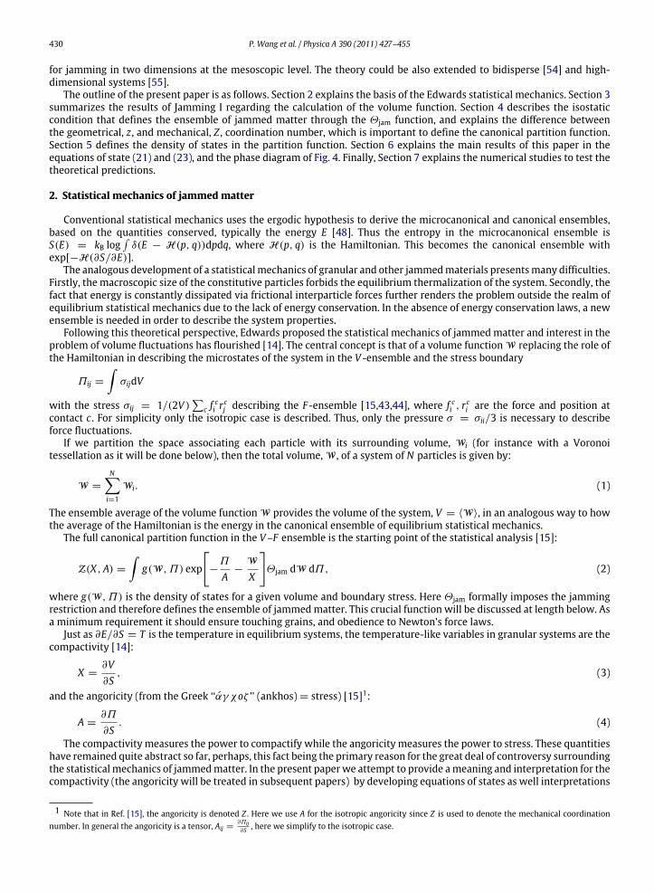
Fig. 2. Mechanical coordination number versus frictionµ obtained in our numerical simulations explained in Section 7 for different preparation protocolscharacterized by the initial volume fractions φi indicated in the figure. The symbols and parameters used in these simulations are the same as in the plotof Fig. 11.
In the following, we present a rough approximation suggesting that the coordination number could be related to friction.We consider the following argument. Consider a set of spherical particles interacting via normal and tangential contactforces. These can be the standard Hertz and Mindlin/Coulomb forces of contact mechanics [35,36,30], respectively, seeSection 7.1. We set N: number of particles, Nn: number of unknown normal forces, Nt : number of unknown tangentialforces, Ef : number of force balance equations, Et : number of torque balance equations, Z = 2M/N: average coordinationnumber of the packing, where M is the total number of contacts, f1(µ): undetermined function of the friction coefficient µsuch that 1 − f1(µ) is the fraction of spheres that can rotate freely (f1(0) = 0 and f1(∞) = 1), and f2(µ): undeterminedfunction of µ indicating the ratio of contacts satisfying Ft < µFn, which satisfies f2(0) = 0 and f2(∞) = 1.
A packing is isostatic when
Nn + Nt = Ef + Et . (9)
The average coordination number at the isostatic point is then (see Table 1):
Z(µ) = 2d1 + 1/2(d − 1)f1(µ)
1 + (d − 1)f2(µ), (10)
reducing to the known Z = 2d for frictionless particles and Z = d + 1 for infinitely rough particles.In what follows, we use the numerical fact that interpolating between the two isostatic limits, there exist packings of
finite µ with the coordination number smoothly varying between Z(µ = 0) = 6 and Z(µ → ∞) → 4 [31]. Numericalsimulations with packings described in Section 7 corroborate this result and further show that the Z vs. µ dependence isindependent of the preparation protocol as obtained in our simulations (see Fig. 2). This result then generalizes the isostaticconditions from µ = 0 and µ = ∞ to finite µ.
It should be noted that we cannot rule out that other preparation protocols could give rise to other dependence of Z onµ. However, we will see that the obtained phase diagram is given in terms of Z; the main prediction of the theory wouldstill be valid irrespective of the particular dependence Z(µ). That is, the theory does not assume anything about the relationbetween the interparticle friction and Z .
It is worth noting that other attempts to define the jammed state have been developed. A rigorous attempt is that ofTorquato et al. who propose three categories of jamming [62]: locally jammed, collectively jammed and strictly jammedbased on geometrical constraints. However, the definition of Ref. [62] is based purely on geometrical considerations andtherefore only valid for frictionless particles. Thus it is not suitable for granular materials with inter-particle frictionaltangential forces; their configurational space is influenced by the mechanics of normal and shear forces. Other approachesto define a jammed state based on the potential energy landscape [28] fail for granular materials too since such a potential

434 P. Wang et al. / Physica A 390 (2011) 427–455
Isostatic packing
a b
Fig. 3. (a) Consider a frictionless packing at the isostatic limit with z = 6. In this case the isostatic condition implies also Z = 6mechanical forces from thesurrounding particles. (b) If we now switch on the tangential forces using the same packing as in (a) by setting µ → ∞, the particle requires only Z = 4contacts to be rigid. Such a solution is guaranteed by the isostatic condition for µ → ∞. Thus, the particle still have z = 6 geometrical neighbors but onlyZ = 4 mechanical ones.
Fig. 4. Phase diagram of jammed matter: theory. Theoretical prediction of the statistical theory. All disordered packings lie within the yellow triangledemarcated by the RCP line, RLP line and G line. Lines of finite isocompactivity are in colour. The grey area is the forbidden zone where no jammedpackings can exist. (For interpretation of the references to colour in this figure legend, the reader is referred to the web version of this article.)
does not exist for frictional grains due to their inherent path-dependency. Thus, the definition of jammed state for granularmaterials must consider interparticle normal and tangential contact forces beyond geometry. In the companion paper [51]we elaborate on this problem.
4.1. Geometrical and mechanical coordination numbers
We have acknowledged a difference between the geometrical coordination number z in Eq. (7) and the mechanicalcoordination number Z which counts only the contacts with nonzero forces. Below we discuss the bounds of z.
Since some geometrical contacts may carry no force, then we have:
Z ≤ z. (11)
To show this, imagine a packing of infinitely rough (µ → ∞) spheres with volume fraction close to 0.64. There must bez = 6 nearest neighbors around each particle on the average. However, the mechanical balance law requires only Z = 4contacts per particle on average, implying that 2 contacts have zero force and do not contribute to the contact force network.
Such a situation is possible as shown in Fig. 3: starting with the contact network of an isostatic packing of frictionlessspheres having Z = 6 and all contacts carrying forces (then z = 6 also as shown in Fig. 3(a)), we simply allow the existenceof tangential forces between the particles and switch the friction coefficient to infinity. Subsequently, we solve the force andtorque balance equations again for this modified packing of infinitely rough spheres but the same geometrical network, asshown in Fig. 3(b). (Notice that the shear force is composed of an elastic Mindlin component plus the Coulomb conditiondetermined by µ, see Section 7.1 for details. Thus when µ → ∞, the elastic Mindlin component still remains.)
The resulting packing is mechanically stable and is obtained by setting to zero the forces of two contacts per ball, onaverage, to satisfy the new force and torque balance condition for the additional tangential force at the contact. Such asolution is guaranteed to exist due to the isostatic condition: at Z = 4 the number of equations equals the number of force

P. Wang et al. / Physica A 390 (2011) 427–455 435
variables. Despite mechanical equilibrium, giving Z = 4, there are still z = 6 geometrical contacts contributing to thevolume function.
Therefore, we identify two types of coordination number: the geometrical coordination number, z, contributing to thevolume function and themechanical coordination number, Z , measuring the contacts that carry forces only. This distinctionis crucial to understand the sum over the states and the bounds in the partition function as explained below.
These ideas are corroborated by numerical simulations in Section 7.6. The packings along the vertical RCP line found inthe simulations (see Fig. 11) have approximately the same geometrical coordination number, z ≈ 6. However, they differin mechanical coordination number, going from the frictionless point Z = 6 to Z ≈ 4 as the friction coefficient is increasedto infinity.
We have established a lower bound of the geometrical coordination in Eq. (11). The upper bound arises from consideringthe constraints in the positions of the rigid hard spheres. For hard spheres, theNd positions of the particles are constrained bythe Nz/2 geometrical constraints, |rij| = 2R, of rigidity. Thus, the number of contacts satisfies Nz/2 ≤ Nd, and z is boundedby:
z ≤ 2d. (12)
Notice that this upper bound applies to the geometrical coordination, z and not to the mechanical one, Z , and it is valid forany system irrespective of the friction coefficient, from µ = 0 → ∞.
Furthermore, in relation with the discussion of frictionless isostaticity, it is believed that above 2d, the system is partiallycrystallized. To increase the coordination number above 6, it is necessary to create partial crystallization in the packing,up to the point of full order of the FCC lattice with coordination number 12. Thus, by defining the upper bound at thefrictionless isostatic limit we also exclude from the ensemble the partially crystalline packings. This is an important point,akin to mathematical tricks employed in replica approaches to glasses [38].
In conclusion, themechanical coordination number, Z , ranges from4 to 6 as a function ofµ, and provides a lower bound tothe geometrical coordination number,while the upper bound is 2d. A granular system is specified by the interparticle frictionwhich determines the average mechanical coordination at which the system is equilibrated, Z(µ). The possible microstatesin the ensemble available for this system follow a Boltzmann distribution Eq. (5) for states satisfying the following bounds:
Z(µ) ≤ z ≤ 2d = 6. (13)
5. Density of states
According to the statistical mechanics of jammed matter, the volume partition function Z is defined by Eq. (5). In thequasiparticle approximation we can write:
Zhardsph (X) =
∫. . .
∫g
−w(zi)
e−
∑w(zi)/XΘjam
N∏i
dw(zi). (14)
Considering N non-interacting quasiparticles with free volume w(z), the partition function can be written as:
Zhardsph =
∫g(w) e−w/XΘjam dw
N
. (15)
Here, g(w) is the density of states for a given quasiparticle free volume.Since the mesoscopic w is directly related to z through Eq. (7), we change variables to the geometrical coordination
number in the partition function. The density of states for a single quasiparticle, g(w), is:
g(w) =
∫ 6
ZP(w|z)g(z)dz, (16)
where P(w|z) is the conditional probability of a free volume w for a given z, and g(z) is the density of states for a given z.Here, we have used the bounds in Eq. (13).
The next step in the derivation is the calculation of g(z) which is developed in three steps.First, we consider that the packing of hard spheres is in a jammed configuration where there can be no collective
motion of any contacting subset of particles leading to unjamming when including the normal and tangential forcesbetween the particles. This definition is an extended version of the collectively jammed category proposed by Torquatoand Stillinger [62] that goes beyond the merely locally jammed configuration of packings, unstable to the motion of a singleparticle. While the degrees of freedom are continuous, the fact that the packing is collectively jammed implies that thejammed configurations in the volume space are not continuous. Otherwise there would be a continuous transformation inthe position space that would unjam the system contradicting the fact that the packing is collectively jammed.
Thus, we consider that the configuration space of jammed matter is discrete since we cannot change one configurationto another in a continuous way. Similar consideration of discreteness has been studied in Ref. [62]. Notice that the volume

436 P. Wang et al. / Physica A 390 (2011) 427–455
landscape could be continuous since we could change the volume as well, or, in the case of soft particles, we can deformthem. Additionally, in the case of frictionless packings of soft particles, the energy of deformation iswell-defined, andwe candefine the collectively jammed configuration as a minimum in the energy with definitive positive Hessian (or a zero ordersaddle) like in Ref. [28]. In this case, there could be no continuous transformation of the particle coordinates that brings onejammed state to the next, unless we deform the particles. Thus, the space is discrete in this case as well.
Second, we call the dimension per particle of the configuration space as D and consider that the distance between twojammed configurations is not broadly distributed (meaning that the average distance is well-defined). We call the typical(average) distance between configurations in the volume space as hz , and therefore the number of configurations per particleis proportional to 1/(hz)
D . The constant hz plays the role of the Planck’s constant, h, in quantum mechanics.Third, we add z constraints per particle due to the fact that the particle is jammed by z contacts. Thus, there are Nz
position constraints (|rij| = 2R) for a jammed state of hard spheres as compared to the unjammed ‘‘gas’’ state. Therefore,the number of degrees of freedom is reduced to D − z, and the number of configurations is then 1/(hz)
D−z . Since the term1/(hz)
D is a constant, it will not influence the average of the observables in the partition function (although it changes thevalue of the entropy, see Jamming III [51]). Therefore, the density of states g(z) is assumed to have an exponential form:
g(z) = (hz)z= e−z/zc , (17)
with z−1c ≡ ln(1/hz). Physically, we expect hz ≪ 1, then g(z) is an exponentially rapid decreasing functionwith z. The exact
value of hz can be determined from a fitting of the theoretical values to the simulation data. The most populated state is thehighest volume at z = 4 while the least populated state is the ground state at z = 6. A constant could be added in (17) but ithas no consequence for the average of the observables in the partition function. However, it affects the value of the entropy.For the calculation of the entropy we consider that there is a single mesoscopic ground state and use g(z) = e−(z−2d)/zc [51].
We see that the negative of the geometrical coordination number,−z, plays the role of a number of degrees of freedom fora packing, due to the extra position constraints of the contacting particles. The coordination z can be then considered as thenumber of degrees of ‘‘frozen’’ per particle. Another way to understand Eq. (17) is the following. In the case of a continuousphase space of configurations we would obtain g(z+1)
g(z) = 0. However, since the space of volume configurations is discrete as
discussed above, the ratio g(z+1)g(z) ∼ hz . This implies again Eq. (17).
The conditional probability P(w|z) depends on the w function, w =2√3
z . The average is taken over a certain mesoscopiclength scale since the volume of a particle depends on the positions of the particles surrounding it. Practically, such lengthscale is approximately of several particle diameters. w is a coarse-grained volume and independent of the microscopicpartition of the particles, implying:
P(w|z) = δ(w − 2√3/z). (18)
Themeaning of Eq. (18) is that we neglect the fluctuations in the coordination number due to the coarse graining procedure.A more general ensemble can be considered where the fluctuations in the geometrical coordination number are taken intoaccount. We have extended our calculations to consider fluctuations in z and find a similar phase diagram as predicted bythe present partition function. This generalized z-ensemble will be treated in a future paper, where the boundaries of thephase diagram are regarded as a second-order phase transition. The generalized z-ensemble allows for the calculation of theprobability distribution of the coordination number, beyond the assumption of the delta function distribution in Eq. (18).The resulting prediction of P(z) is in general agreement with simulations (see Ref. [52]).
Substituting Eqs. (18) and (17) into Eq. (15), we find the isostatic partition function which is used in the remainder of thisstudy:
Ziso(X, Z) =
∫ 6
Z(hz)
z exp
−
2√3
zX
dz. (19)
6. Phase diagram
Next, we obtain the equations of state to define the phase diagram of jammed matter by solving the partition function.From Eq. (19), we calculate the ensemble average volume fraction φ = (w + 1)−1
= z/(z + 2√3) as:
φ(X, Z) =1
Ziso(X, Z)
∫ 6
Z
z
z + 2√3exp
−
2√3
zX+ z ln hz
dz. (20)
We start by investigating the limiting cases of zero and infinite compactivity.(a) In the limit of vanishing compactivity (X → 0), only the minimum volume or ground state at z = 6 contributes to
the partition function. Then we obtain the ground state of jammed matter with a density:
φRCP = φ(X = 0, Z) =6
6 + 2√3
≈ 0.634, Z(µ) ∈ [4, 6]. (21)
The meaning of the subscript RCP in (21) will become clear below.

P. Wang et al. / Physica A 390 (2011) 427–455 437
(b) In the limit of infinite compactivity (X → ∞), the Boltzmann factor exp[−2√3/(zX)] → 1, and the average in (20)
is taken over all the states with equal probability. We obtain:
φRLP(Z) = φ(X → ∞, Z)
=1
Ziso(∞, Z)
∫ 6
Z
z
z + 2√3exp (z ln hz) dz. (22)
The constant hz determines the minimum volume in the phase space. We expect hz ≪ 1, such that the exponential inEq. (22) decays rapidly. Then the leading contribution to Eq. (22) is from the highest volume at z = Z and therefore:
φRLP(Z) ≈Z
Z + 2√3, Z(µ) ∈ [4, 6]. (23)
This dependence of the volume fraction on Z suggests using the (φ, Z) plane to define the phase diagram of jammedmatter as plotted in Fig. 4. The equations of state (21) and (23) are plotted in the (φ, Z) plane in Fig. 4 providing two limitsof the phase diagram. Since the mechanical coordination number is limited by 4 ≤ Z ≤ 6 we have two more horizontallimits. The phase space is delimited from below by the minimum coordination Z = 4 for infinitely rough grains, denotedthe granular-line or G-line in Fig. 4.
Allmechanically stable disordered jammedpackings liewithin the confining limits of the phase diagram (indicated by theyellow zone in Fig. 4), while the grey shaded area in Fig. 4 indicates the forbidden zone. For example, a packing of frictionalhard spheres with Z = 5 (corresponding to a granular material with interparticle friction µ ≈ 0.2 according to Fig. 2)cannot be equilibrated at volume fractions below φ < φRLP(Z = 5) = 5/(5+ 2
√3) = 0.591 or above φ > φRCP = 0.634. It
is worth noting that particular packings can exist in the forbidden zone; our contention is that they are zero measure andtherefore have zero probability of occurrence at the ensemble level.
These results provide a statistical interpretation of the RLP and RCP limits.(i) The RCP limit—Stemming from the statistical mechanics approach, the RCP limit arises as the result of the relation (21),
which gives themaximum volume fraction of disordered packings under themesoscopic framework. To the right of the RCPline, packings exist only with some degree of order (for instance with crystalline regions). The prediction,
φRCP =6
6 + 2√3
≈ 0.634, (24)
is valid for all friction coefficients and approximates the experimental and numerical estimations [5–8] which find a closepacking limit independent of friction in a narrow range around 0.64.
Beyond the fact that 63%–64% is commonly quoted as RCP for monodisperse hard spheres, we present a physicalinterpretation of that value as the ground state of frictional hard spheres characterized by a given interparticle frictioncoefficient. In this representation, as µ varies from 0 to ∞ and Z decreases from 6 to 4, the state of RCP changes accordinglywhile its volume fraction remains the same, given by Eq. (24). The present approach has led to an unexpected number ofstates that all lie in the RCP line from Z = 6 to Z = 4 as depicted in Fig. 4, suggesting that RCP is not a unique point in thephase diagram.
An important prediction is that for frictionless systems there is only one possible state at Z = 6. It is important to notethat there is one state only at the mesoscopic level used in the theory. However, for a single mesoscopic state, we expectmany microstates, which are averaged out in the mesoscopic theory of the volume function. Thus, there could be morejammed states surrounding the frictionless point in the phase diagram. However, we expect that these states are clusteredin a narrow region around the frictionless point. To access thesemicrostates it would require different preparation protocols,analogous to the dependence of the glass transition temperature on cooling rates in glasses [40,38].
It is interesting to note that replica approaches to the jammed states [38] predict many jammed isostatic states withdifferent volume fractions for frictionless hard spheres. The first question is whether these states in the force/energyensemble are the same as the volume ensemble states that we treat in our approach. It should be noted that jammingin Refs. [40,38] is obtained when the particles are rattling infinitely fast in their cages, in the limit of infinite number ofcollisions per unit time. That is when the dynamic pressure related to the momentum of the particles diverges. Second,from our point of view, an investigation of the fluctuations of the microstates as well as more general ensembles allowingfor fluctuations in the coordination number could be considered. These studies may reveal whether the frictionless point isunique or not. This point is investigated further in Section 7.5.
(ii) The RLP limit—Equation of state (23) provides the lowest volume fraction for a given Z and represents a statisticalinterpretation of the RLP limit depicted by the RLP line in Fig. 4. We predict that to the left of this line, packings are notmechanically stable or they are experimentally irreversible as discussed in Refs. [19,21,20].
A review of the literature indicates that there is no general consensus on the value of RLP as different estimations havebeen reported ranging from 0.55 to 0.60 [6,9,8], proposing that there is no clear definition of RLP limit. The phase diagramproposes a solution to this problem. Following the infinite compactivity RLP line, the volume fraction of the RLP decreaseswith increasing friction from the frictionless point (φ, Z) = (0.634, 6), towards the limit of infinitely rough hard spheres,

438 P. Wang et al. / Physica A 390 (2011) 427–455
Z → 4. Indeed, experiments [6] indicate that lower volume fractions are achieved for larger coefficient of friction. Wepredict the lowest volume fraction in the limit: µ → ∞, X → ∞ and Z → 4 (and hz → 0) at
φminRLP =
4
4 + 2√3
≈ 0.536. (25)
Even though this is a theoretical limit, our results indicate that for µ > 1 this limit can be approximately achieved.The finding of a random loose packing bound is an interesting prediction of the present theory. The RLP limit has not been
well investigated experimentally, and so far it was not certain whether this limit can or cannot be reached in real systems.The lowest stable volume fraction ever reported, 0.550 ± 0.006, obtained by Onoda and Liniger [9] as the limit of vanishinggravity for spherical glass beads, is not far from the present prediction.
The intersections of the RCP, RLP and the G-line identify three interesting points in the (φ, Z(µ)) plane.(a) The frictionless point µ = 0, denoted J-point in Ref. [28], at
J ≡ (φRCP, Z(0)) = (0.634, 6),
corresponds to a system of compressed emulsions in the limit of small osmotic pressure as measured by Brujić [63].(b) The lowest coordination number Z = 4 plotted as the G-line defines two associated points from the lowest volume
fraction of loose packings at infinite compactivity, L-point,
L ≡ (φminRLP , Z(∞)) = (0.536, 4),
to the zero compactivity state of close packing, C-point,
C ≡ (φRCP, Z(∞)) = (0.634, 4).
The full JCL triangle defines the isostatic plane where the frictional hard sphere packings reside.(iii) Intermediate isocompactivity states—For finite X , Eq. (20) can be solved numerically. For each X , the function φ(X, Z)
can be obtained and is plotted as each isocompactivity colour line in Fig. 4. Between the two limits Eqs. (21) and (23), thereare packings inside the yellow zone in Fig. 4 with finite compactivity, 0 < X < ∞. Since X controls the probability of eachstate, like in condensed matter the number of possible ways to rearrange a packing having a given volume and entropy, S.Thus, the limits of themost compact and least compact stable arrangements correspond to X → 0 and X → ∞, respectively.Between these limits, the compactivity determines the volume fraction from RCP to RLP.
Dependence on hz and negative compactivityOf interest is the dependence of our prediction on the ‘‘Planck constant’’ of jammed matter, hz , that determines the
minimum volume in the phase space. The equation of state (23) and the prediction of the minimum RLP, Eq. (25) have beenobtained by considering hz → 0 but still nonzero. Thus, when X → ∞, the only state contributing to the volume partitionfunction is the most populated at z = Z(µ).
The approximation hz ≪ 1 is a sensible one, since the discretization of the space is supposed to be very small. However,this constant remains a fitting parameter of the theory. Indeed in the simulations we will use a value of hz = e−100 in orderto fit the theoretical values with the numerical ones for finite compactivity. This extremely small constant shifts the valueof the minimum RLP a little bit to the right of the phase diagram from the prediction of Eq. (25). Indeed, when we plot thephase diagram of Fig. 4 with a hz = e−100 a slightly larger value of φmin
RLP is obtained as seen in Fig. 4. In the unphysical limit ofhz → 1wewould obtain aminimum RLP value of (φmin
RLP +φRCP)/2, although as said, this would correspond to an unphysicalsituation.
However, it should be noted that this argument depends on the assumed exponential form of the density of states. Sinceat this point we do not have the exact form for the density of states, the results could change if other more accurate densityis found to be valid. On the other hand the prediction of the ground state at RCP, Eq. (21), remains unaffected by the densityof state or the value of hz .
It is interesting to note that we can extend the compactivity to negative values and study the range X : 0−→ −∞.
Indeed, for any value of hz , in the limit X → 0− we obtain the lowest volume fraction of the prediction of Eq. (23).Thus, properly speaking, the minimum value of RLP is defined in the limit of negative zero compactivity, and this limitis independent of the value of hz . The entropy has an interesting behavior in this regime which will be discussed later.
It is important to realize that the region from X : 0−→ ∞ disappears when hz → 0, thus the only meaningful limit is
that of X → +∞ (which equals both the limits X → −∞ and X → 0− when hz → 0). Thus, for any practical purpose,Eq. (25) can be considered to be the lowest possible density predicted by the theory. However, notice that the shape of theiso-compactivity curves depends slightly on the value of hz .
Sincewe always expect hz ≪ 1, it may not be necessary to use the negative compactivity states to describe RLP.We leavethis interesting observation for further investigations where the entropy of jamming is treated in more details in Ref. [51].
6.1. Volume landscape of jammed matter
Eq. (7) plays the role of the Hamiltonian of the jammed system and the jammed configurations can be considered as theminima of (7). Inspired by the physics of glasses and supercooled liquids, we imagine a ‘‘volume landscape’’, analogous to

P. Wang et al. / Physica A 390 (2011) 427–455 439
W
O
d
W
O
b
W
O
c
W
O
a
Fig. 5. Schematic representation of the volume landscape of jammed matter (ri,W ). The multidimensional coordinate ri represents the degrees of freedom:the particle positions. Each dot represents a discrete mesoscopic jammed state at different z. It is important to note that for each meso state there aremicroscopic states with the same z. All disordered packings are in the yellow region (of a schematic shape) of the phase space which corresponds to theisostatic plane of hard spheres at the jamming transition where our calculations are performed. Other ordered packings have lower volume, such as theFCC. (a) We represent the case of µ = ∞. The states represent those along the G-line in Fig. 4 as the compactivity varies from X = 0 (ground state) toX → ∞ at the RLP. The horizontal lines indicate packings at constant volume. The ground state of jammed matter for this friction coefficient has z = 6and the highest volume states are found for z = 4. The arrow indicates the limits of integration in the partition function for this particular friction. (b)For another finite µ, the space is delimited from above by a line of constant z = Z(µ). (c) For µ = 0 only the ground state is available, giving rise to asingle state. (d) The volume states in (a, b, c) are separated by energy barriers represented by the third coordinate in the phase space. The energy barriersare path dependent due to friction between the particles. Nevertheless, the jammed configurations are well-defined in the isostatic plane, and the energybarriers represent the work done to go from one configuration to another. Only at the frictionless point, the energy barriers are path independent. (Forinterpretation of the references to colour in this figure legend, the reader is referred to the web version of this article.)
the energy landscape in glasses [64], as a pictorial representation to describe the states of jammedmatter. Each mesoscopicjammed state (determined by the positions of the particles, denoted ri, and its corresponding volume w) is depicted as apoint in Fig. 5. At the mesoscopic level, the volume landscape has different levels of constant z, analogous to energy levelsin Hamiltonian systems.
The lowest volume corresponds to the FCC/HCP structure (with kissing number z = 12), as conjectured by Kepler [1].Other lattice packings, such as the cubic lattice and tetrahedron lattice, have higher volume levels in this representation.Beyond these ordered states, the ensemble of disordered packings is identified within the yellow area in Fig. 5(a),corresponding to a system with infinite friction. In this case the partition function is integrated from z = 4 to 6, thusall the states are sampled in the configuration average as indicated by the arrow in Fig. 5(a). When X → ∞, all the statesare sampled with equal probability, and, when X → 0, the ground state is the most probable. As the compactivity is varied,the states along the G-line in the phase diagram result. For µ → ∞, the maximum volume, w(z = 4) =
√3/2 is attained
for z = 4 when µ → ∞ in analogy with the high energy states in a classical system.As we set the friction coefficient to a finite value, the available states in the volume are less, since the integration in the
partition function is in the region Z(µ) ≤ z ≤ 6. This is indicated in Fig. 5(b) for a generic Z(µ). Finally when the frictionvanishes, we obtain only the ground state z = 6 as indicated in Fig. 5(c).
For any value of µ, the lowest state is always at z = 6. This corresponds to the states exemplified by the RCP line inthe phase diagram, all of them with a geometrical coordination z = 6. Eq. (21) indicates that the RCP corresponds to theground state of disordered jammed matter for a given friction which determines Z , while the RLP states are achieved forhigher volume levels as indicated in Fig. 5. An important conclusion is the following. The states along the RCP line all havez = 6, independent of Z (and hz) which ranges from 4 to 6 as a function of the friction coefficient µ. The states along theRLP line all have z = Z (when hz → 0). These predictions find good agreement with the numerically generated packings inSection 7.6.
At fixed volume, the jammed states are separated bybarriers of deformation energy, as depicted in Fig. 5(d). These barrierscan be understood as follows: so far we have treated the case of hard spheres considered as soft spheres (interacting via soft-potential such as Hertz–Mindlin forces) in the limit of vanishing deformation or infinite shear modulus. Indeed, the way toconsider forces in granular materials is by considering the small tiny deformation at the contact points and a given force

440 P. Wang et al. / Physica A 390 (2011) 427–455
Fig. 6. Predictions of the equation of state of jammed matter in the (X, φ, s) space. Each line corresponds to a different system with Z(µ) as indicated. Theprojections in the (φ, s) and (X, s) planes show that the RCP (X = 0) is less disordered than the RLP (X → ∞). The projection in the (X, φ) plane resemblesqualitatively the compaction curves of the experiments [19,21,20].
law [30]. In a sense, deformable particles are needed when discussing realistic jammed states especially when consideringthe problem of sound propagation and elastic behavior [65,66]. In the case of deformable particles the third axis in Fig. 5(d)corresponds to the energy of deformation or the work done to go from one configuration to the next. This energy is notuniquely defined in terms of the particle coordinates; it depends on the path taken from one jammed state to the next. Thus,we emphasize that the energy in Fig. 5 is path-dependent. The only point where it becomes independent of the path is inthe frictionless point. Besides this, the volume landscape in the isostatic plane Fig. 5(a)–(c) is well defined and independentof the energy barriers and path dependent issues.
It is important to note that the basins in Fig. 5 are not single states, but represent many microscopic states with differentdegrees of freedom ri, parameterized by a common value of z with a density of states g(z). The basins represent single statesonly at themesoscopic level providing amesoscopic view of the landscape of jammed states. This is an important distinctionarising from the fact that the states defined byw(z) = 2
√3/z, Eq. (7), are coarse grained from themicroscopic states defined
by the microscopic Voronoi volume Eq. (6) in the mesoscopic calculations leading to (7) as discussed in Jamming I [49]. Thisfact has important implications for the present predictions which will be discussed in Section 7.5. The advantage of thevolume landscape picture is that it allows visualization of the corresponding average over configurations that give rise tothe macroscopic observables of the jammed states.
6.2. Equations of state
Further statistical characterization of the jammed structures can be obtained through the calculation of the equations ofstate in the three-dimensional space (X, φ, S), with S the entropy, as seen in Fig. 6.
The entropy density, s =SN , is obtained as:
s(X, Z) = ⟨w⟩/X + lnZiso(X, Z). (26)
This equation is obtained in analogy with equilibrium statistical mechanics and it is analogous to the definition of freeenergy: F = E − TS where F = −T lnZ is the free energy. We replace T → X, E → ⟨w⟩. Therefore, F = E − TS orS = (E − F)/T = E/T + lnZ is now s(X, Z) = ⟨w⟩ /X + lnZiso(X, Z), which is plotted as the equation of state in Fig. 6.
Each curve in the figure corresponds to a systemwith a different Z(µ). The projections S(X) and S(φ) in Fig. 6 characterizethe nature of randomness in the packings. When comparing all the packings, the maximum entropy is at φmin
RLP and X → ∞
while the entropy is minimum for φRCP at X → 0. Following the G-line in the phase diagram we obtain the entropy forinfinitely rough spheres showing a larger entropy for the RLP than the RCP. The same conclusion is obtained for the otherpackings at finite friction (4 < Z(µ) < 6). We conclude that the RLP states are more disordered than the RCP states.Approaching the frictionless J-point at Z = 6 the entropy vanishes. More precisely, it vanishes for a slightly smaller φ thanφRCP of the order hz . Strictly speaking, the entropy diverges to −∞ at φRCP as S → ln X for any value of Z , in analogy withthe classical equation of state, when we approach RCP to distances smaller than hz . However, this is an unphysical limit, asit would be like considering distances in phase space smaller than the Planck constant.
It is commonly believed that the RCP limit corresponds to a statewith the highest number of configurations and thereforethe highest entropy. However, herewe show that the stateswith a higher compactivity have a higher entropy, correspondingto looser packings. Within a statistical mechanics framework of jammed matter, this result is a natural consequence andgives support to such an underlying statistical picture. Amore detailed study of the entropy is performed in Jamming III [51].

P. Wang et al. / Physica A 390 (2011) 427–455 441
The interpretation of the RCP as the ground state, X → 0, with vanishing entropy (S → 0 and therefore a unique state)warrants an elaboration. We notice that there exist packings above RCP all the way to φFCC = 0.74048, but these packingshave some degree of order. These partially ordered packings do not appear in our theory because we treat only disorderedpackings characterized by the mesoscopic volume function which has been derived under the isotropic assumption. Bydoing so, we explicitly do not consider crystals or partially crystalline packings in the ensemble. This interprets the RCP inthe context of the found third-law of thermodynamics. Our approach of neglecting the crystal state from the ensemble hasanalogies in replica treatment of glasses [67].
The mesoscopic entropy vanishes at RCP. From this point the entropy increases monotonically with X , being maximumfor the RLP limit. We note that the microscopic states contribute still to the entropy of RCP giving rise to more states thanpredicted by the present mesoscopic approach. This case is discussed in more detail in Ref. [51].
The equation of state φ(X) for different values of Z can be seen in the projection of Fig. 6. The volume fraction diminisheswith increasing compactivity according to the theoretical picture of the phase diagram. The curves φ(X) qualitativelyresemble the reversible branch of compaction curves in the experiments of Ref. [19] for shaken granular materials andoscillatory compression of grains [20] suggesting a correspondence between X and shaking amplitude. The intention is thatdifferent control parameters in experiments could be related to a state variable, and therefore might help experimentaliststo describe results obtained under different protocols.
For any value of Z , there is a common limit φ → φRCP as X → 0, indicating the constant volume fraction for all the RCPstates. The singular nature of the frictionless J-point is revealed as the volume fraction remains constant for any value ofX , explaining why this point is the confluence of the isocompactivity lines, including RCP and RLP. We conclude that at thefrictionless J-point the compactivity does not play a role, at least at the mesoscopic level.
6.3. Experimental realization of the phase diagram
A reanalysis of the available experimental data tends to agree with the above theoretical predictions. However, it wouldbe desirable to perform more controlled experiments in light of the present results. As in other out of equilibrium systems,such as glasses, the inherent path-dependency of jammed matter materializes in the fact that different packing structurescan be realized with different preparation protocols [18,19,21,20,42] involving tapping, fluidized beds, settling particles atdifferent speeds, acoustic perturbations or pressure waves [9]. Due to this reason, the value of φRCP has not been determinedyet for monodisperse frictionless systems. The more extensive evidence for a frictionless RCP appears from simulations,which have been extensively performed for hard and soft sphere systems. They find a common value of RCP for manydifferent preparation protocols [27,28,40]. For frictional materials, experiments of Scott and Kilgour [6], and others displaya nearly universal value of volume fraction for RCP consistent with the theoretical estimation.
Previous experiments [9] and simulations [30] find that lower volume fractions can be achieved for smaller settlingspeeds of the grains or slower compression (or quenching) rates during packing preparation. Colloidal glasses find a similarscenario [38,41], with their glass transition temperature dependence on the quench rate of cooling, although due to differentreasons. This raises the question of whether the jamming point is unique or determined by the preparation protocol [41].
The experiments performed by Onoda and Liniger with glass spheres in liquid of varying density to adjust conditionsof buoyancy in the limit of vanishing gravity show that for larger values of gravity, the volume fraction decreases. Thisindicates that settling speed of the particles can determine the final volume fraction. Indeed, it was found numerically thatthe compression rate during preparation of the packings is a systematic way to obtain lower packing fractions, such thatlower volume fractions can be achieved with quasi-static compression rates during preparation of the packings [30].
On the other hand, measuring the mechanical coordination number in experiments seems to be an even more difficulttask. In the phase diagram, the RCP can be found at the frictionless point with the highest possible coordination numberZ = 6. Such a value of Z has been observed in the experiments of Brujić et al. on concentrated emulsions near the jammingtransition [63] and simulations of droplets.
The experiments of Bernal [4] simultaneously measured the coordination number and the volume fraction. Indeed,Mason, a postgraduate student of Bernal, took on the task of shaking glass balls in a sack and freezing the packing by pouringwax over thewhole system.Hewould then carefully take the packing apart, ball by ball, painstakingly recording the positionsof contacts for each of over 8000 particles [4]. Their result is a coordination number Z ≈ 6 and a volume fraction φ ≈ 0.64which corresponds to the prediction of the frictionless point in the phase diagram. This may indicate that the particles usedin the experiment of Bernal have a low friction coefficient.
Another explanation, more plausible, is that the coordination number measured by Bernal is not the mechanical one, butthe geometrical one. Indeed, wemay argue that the only coordination that can bemeasured in experiments of counting balls‘a la Bernal’ is the geometrical one, since, one is never sure if the contacting balls were carrying a force or not. Bernal couldonly measure geometries, not forces. This is in addition to the uncertainty in the determination of the contacts with such arudimentary method as pouring wax and then counting one by one the area of contact. The theory predicts that along theRCP line, all the RCP states have geometrical z = 6, while Z ranges from4 to 6. Thus, it is quite plausible that the coordinationnumber in Bernal experiments is the geometrical one, z = 6, in agreement with the theory.
It is worth noting that since the labor-intensive method patented half a century ago by Bernal, other groups haveextracted data at the level of the constituent particles using X-ray tomography [45]. Such experimentsmay give a clue to therelationship between coordination number and volume fraction. The experimental data, to date, seems in good agreement
442 P. Wang et al. / Physica A 390 (2011) 427–455
with the present theory. However, this method does not directly determine the contacts to verify whether the particles aretouching or just very close together. Furthermore, themethod cannotmeasure forces so the distinction between geometricaland mechanical coordination is not possible to achieve in this experiment.
An answer might be obtained using methods from biochemistry being developed at the moment [68]. These methodspromise to provide the high resolution to determine the contact network with accuracy to develop an experimentalunderstanding of the problem.
An alternatewaymight be generating the packings in the phase space throughnumerical simulations,where both volumefraction and coordination number could be easily determined. Since Z is directly determined by µ, and the compactivitydetermines what value of the volume fraction a packing has between the limits of the phase diagram, the main question ishow to generate packings with different φ for a fixed µ to allow the exploration of the phase diagram.
7. Numerical tests
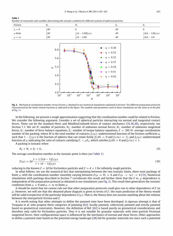
In this section we perform two different numerical tests: on the predictions of the theory and the assumptions of thetheory. The former are explained in Section 7.3 while the latter are elaborated in Section 7.6. It is worth mentioning thatwhile the predictions can be tested with packings prepared numerically and experimentally, the test of the assumptions ofthe theory is not so trivial. This is because the theory is based on the existence of quasiparticles which carry the informationat a mesoscopic scale. Thus, in principle we cannot use real packings, such as computer generated packings or experimentalones, to measure the quasiparticles. The information obtained from those packings already contains ensemble averagesthrough the Boltzmann distribution and density of states. That is, it is in principle not possible to isolate the behavior ofquasiparticles from the real measures rendering it difficult to properly test some of the assumptions of the theory at themore basic mesoscopic scale. In Section 7.6 we attempt to perform such a test, especially since we can easily obtain thepackings at the RLP line or the infinite compactivity limit. These packings are fully random obtained as flat averages in theensemble without the corresponding Boltzmann factor and may contain direct information on the mesoscopic fluctuations.
The existence of the theoretically inferred jammed states opens such predictions to experimental and computationalinvestigation. We numerically test the predictions of the phase diagram by preparing monodisperse packings ofHertz–Mindlin [35,36] spheres with friction coefficient µ at the jamming transition using methods previously developed[27,30,65,66].
We test the theoretical predictions and show how to dynamically generate all the packings in the phase space ofconfigurations through different preparation protocols. Although diverse states are predicted by the theory, theymay not beeasily accessible by experimentation due to their low probability of occurrence. For instance, we will find that the packingsclose to the C-point (high volume fraction, high friction, low coordination) are the most difficult to obtain.
The advantage of our theoretical framework is that it systematically classifies the different packings into a coherentpicture of the phase diagram. In the following we use different preparation protocols to generate all the phase space ofjamming. In particular we provide a scheme to reproduce the RCP and RLP lines amenable to experimental tests.
We achieve different packing states by compressing a system from an initial volume fraction φi with a compression rateΓ in a medium of viscosity (damping) η where the particles are dispersed. The system is defined by the friction coefficientµ which sets Z(µ) according to Fig. 2. While the simulations are not realistic (no gravity, boundaries, or realistic protocolare employed), they provide a way to test themain predictions of the theory. The final state (φ, Z) is achieved by the systemfor every (φi, Γ , η, µ) at the jamming transition of vanishing stress with a method explained next.
It should be noted that other experimental protocols could be also adapted to the exploration of the phase diagram, in-cluding (a) gentle tappingwith servomechanisms that adjust the system at a specified pressure [66], (b) gentle tappingwithexternal oscillatory perturbations, (c) settling of grains under gravity in a variety of liquidswith viscosityη, (d) fluidized beds.
Relation with hard sphere simulations. The present algorithm finds analogies with recent attempts to describe jammingusing ideas coming from the theory of mean-field spin glasses and optimization problems [38,41]. This is an interestingsituation since it has been shown that in the case of hard spheres the system always crystallizes unless an infinite quenchis applied [10].
However, our soft sphere simulations do not produce appreciable crystallization in the packing. This situation can beunderstood as follows. In order to avoid the (partial) crystallization in practice, a fast compression is needed. A simpledimensionality analysis tells that the quenching rate Γ ∝ G1/2, where G is the shear modulus of the grains (see Fig. 7). Thisanalysis allows for comparison of our soft ball simulations with the hard sphere simulations used in other studies [10]. Onecould imagine that there exists a typical quench rate, depending on the stiffness of the grains, as a division of the orderedand disordered (jammed) phases. It is interesting to note that at the hard-sphere limit, G → ∞, all the packings are in theordered phase except when Γ → ∞, where φ ≈ 0.64. This explains the behavior of the hard sphere packings found inpreviousworks [10]. For the soft ball case, the situation ismore subtle since a certain range of compression rate is acceptablefor the acquisition of disordered packings. It is in this range that we perform simulations. However, it should be noted thatthe above simple dimensionality analysis does not consider the dependence on dimensions and algorithms, which probablyhas important effects in the real situation.
According to this picture, in the theoretical limit of infinitely slow quench rates, the system should in principle crystallizefor any G. However in practice, this limit is almost impossible to achieve experimentally. For sufficiently fast quench rates,crystallization can be avoided and a granular system is stuck in a random jammed configuration since its configurational
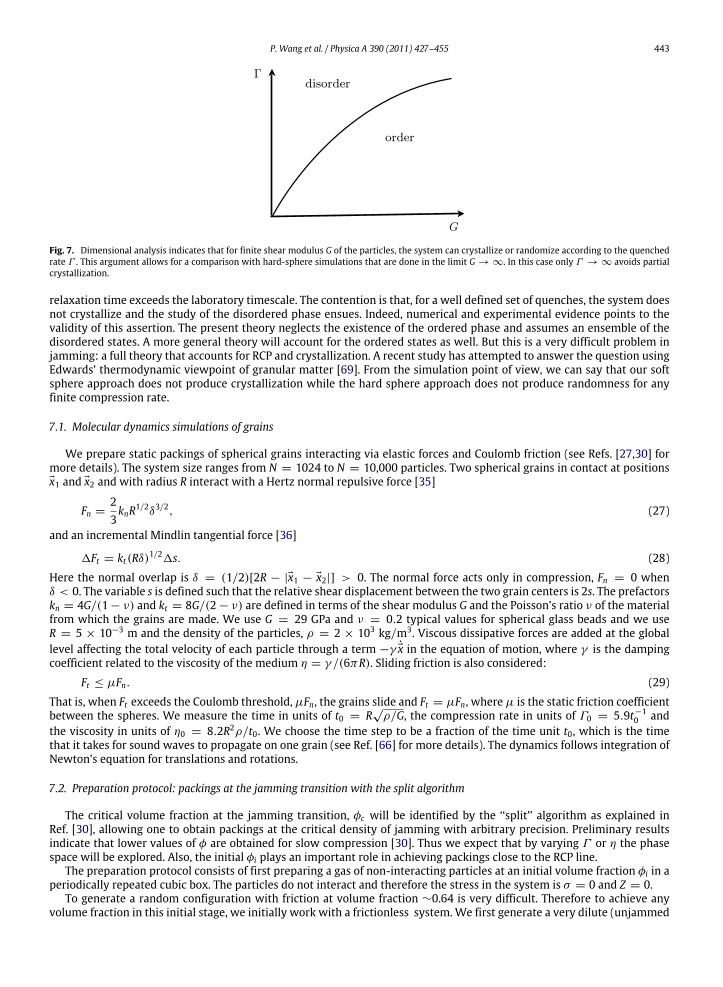
P. Wang et al. / Physica A 390 (2011) 427–455 443
Fig. 7. Dimensional analysis indicates that for finite shear modulus G of the particles, the system can crystallize or randomize according to the quenchedrate Γ . This argument allows for a comparison with hard-sphere simulations that are done in the limit G → ∞. In this case only Γ → ∞ avoids partialcrystallization.
relaxation time exceeds the laboratory timescale. The contention is that, for a well defined set of quenches, the system doesnot crystallize and the study of the disordered phase ensues. Indeed, numerical and experimental evidence points to thevalidity of this assertion. The present theory neglects the existence of the ordered phase and assumes an ensemble of thedisordered states. A more general theory will account for the ordered states as well. But this is a very difficult problem injamming: a full theory that accounts for RCP and crystallization. A recent study has attempted to answer the question usingEdwards’ thermodynamic viewpoint of granular matter [69]. From the simulation point of view, we can say that our softsphere approach does not produce crystallization while the hard sphere approach does not produce randomness for anyfinite compression rate.
7.1. Molecular dynamics simulations of grains
We prepare static packings of spherical grains interacting via elastic forces and Coulomb friction (see Refs. [27,30] formore details). The system size ranges from N = 1024 to N = 10,000 particles. Two spherical grains in contact at positionsx1 and x2 and with radius R interact with a Hertz normal repulsive force [35]
Fn =23knR1/2δ3/2, (27)
and an incremental Mindlin tangential force [36]
1Ft = kt(Rδ)1/21s. (28)
Here the normal overlap is δ = (1/2)[2R − |x1 − x2|] > 0. The normal force acts only in compression, Fn = 0 whenδ < 0. The variable s is defined such that the relative shear displacement between the two grain centers is 2s. The prefactorskn = 4G/(1 − ν) and kt = 8G/(2 − ν) are defined in terms of the shear modulus G and the Poisson’s ratio ν of the materialfrom which the grains are made. We use G = 29 GPa and ν = 0.2 typical values for spherical glass beads and we useR = 5 × 10⁻³ m and the density of the particles, ρ = 2 × 10³ kg/m3. Viscous dissipative forces are added at the globallevel affecting the total velocity of each particle through a term −γ ˙x in the equation of motion, where γ is the dampingcoefficient related to the viscosity of the medium η = γ /(6πR). Sliding friction is also considered:
Ft ≤ µFn. (29)
That is, when Ft exceeds the Coulomb threshold, µFn, the grains slide and Ft = µFn, where µ is the static friction coefficientbetween the spheres. We measure the time in units of t0 = R
√ρ/G, the compression rate in units of Γ0 = 5.9t−1
0 andthe viscosity in units of η0 = 8.2R2ρ/t0. We choose the time step to be a fraction of the time unit t0, which is the timethat it takes for sound waves to propagate on one grain (see Ref. [66] for more details). The dynamics follows integration ofNewton’s equation for translations and rotations.
7.2. Preparation protocol: packings at the jamming transition with the split algorithm
The critical volume fraction at the jamming transition, φc will be identified by the ‘‘split’’ algorithm as explained inRef. [30], allowing one to obtain packings at the critical density of jamming with arbitrary precision. Preliminary resultsindicate that lower values of φ are obtained for slow compression [30]. Thus we expect that by varying Γ or η the phasespace will be explored. Also, the initial φi plays an important role in achieving packings close to the RCP line.
The preparation protocol consists of first preparing a gas of non-interacting particles at an initial volume fraction φi in aperiodically repeated cubic box. The particles do not interact and therefore the stress in the system is σ = 0 and Z = 0.
To generate a random configuration with friction at volume fraction ∼0.64 is very difficult. Therefore to achieve anyvolume fraction in this initial stage, we initially work with a frictionless system. We first generate a very dilute (unjammed

444 P. Wang et al. / Physica A 390 (2011) 427–455
Fig. 8. Schematic representation of the protocol used to dynamically achieve the packings in the phase diagram. (a) The region near the C-point (highfriction, high volume fraction) is the most difficult to access. Here, we prepare an unjammed sample with no friction at φi (=0.62 in the diagram) veryclose to RCP, and then we switch friction to compress to the required frictional jammed state. The packings follow the paths indicated in the figure fortwo friction coefficients. On the other hand, the RLP line is easily obtained by compressing unjammed packings with low φi (=0.52 in the diagram) at (b)a given compression rate Γ1 for a given friction coefficient. (c) There is a small dependence on Γ , the faster the compression the deeper we enter in thephase diagram.
Fig. 9. Time evolution of stress (the pressure in the system) for two packings simulated as explained in the text. The solid red line represents a packingwith φ1 > φc and dotted black line represents a packing with φ2 < φc , where φ1 = φ2 + 2× 10⁻⁴ . The inset shows the time evolution of the coordinationnumber (For interpretation of the references to colour in this figure legend, the reader is referred to the web version of this article.)
gas of non-interacting particles) grain configuration randomly, usually with a volume fraction φ0 ≈ 0.30–0.36. Then weapply an extremely slow isotropic compressionwithout friction on this dilute configuration until the system reaches anotherunjammed configuration at higher density, φi (see Fig. 8(a)). The reason to add an extremely slow isotropic compression tothe dilute configuration is to avoid involving any kinetic energy to keep the system as random as possible. After obtainingthis unjammed state with initial volume fraction φi, we restore friction and a compression is applied with a compressionrate Γ until a given volume fraction φ1. Then the compression is stopped and the system is allowed to relax to mechanicalequilibrium by following Newton’s equations without further compression.
After the compression, two things can occur (see Fig. 9).(a) The system jams. If the volume fraction φ1 is above the jamming point, φ1 > φc , then the stress will decrease
and ultimately stabilize to a finite nonzero value, meaning that the pressure of the system remains unchanged (usually1σ < 10−3 Pa, red line, Fig. 9) over a large period of time (usually ∼107 MD steps). The coordination number usually has afirst initial decrease, but if the system is jammed it will also stabilize at a constant value above the isostatic minimal number(inset Fig. 9).
(b) The system is not jammed. If the volume fraction φ2 is below the jamming point, φ2 < φc , then the stress andthe coordination number will relax to zero. This fact is illustrated in Fig. 9. If the packing has φ1 > φc , it stabilizes at a

P. Wang et al. / Physica A 390 (2011) 427–455 445
Stable
Stable?
Unstable
yesno
Fig. 10. Flow chart for searching procedure of critical volume fraction φc .
a
b
Fig. 11. Phase diagram of jammed matter: simulations. Numerical simulations demonstrate how to dynamically access the theoretically found states. Thenumerical protocol is parameterized by (φi, Γ , η, µ). (a) The plot shows the dependence of the final jammed states (φ, Z) on φi for a fixed Γ = 10−7 andη = 10−3 (except for the orange I curve which is for η = 10−4) from left to right φi = 0.40 (black �), 0.53 (red •), 0.55 (violet N), 0.57 (blue H), 0.59 (green�), 0.61 (pink J) and 0.63 (orange I). Each equal-colour line set represents a different φi and the dashed lines join systems with the same friction µ. Solidlines represent the theoretical results with hz = e−100 or zc = 0.01 for different compactivities measured in units of 10−3Vg . From left to right X = ∞
(black solid line), 1.62 (blue solid line), 1.38 (green solid line), 1.16 (pink solid line) and 0.88 (orange solid line). The error bars correspond to the s.d. over10 realizations of the packings. (b) The plot focuses on the dependence of (φ, Z) on (Γ , η) for two different φi . Solid black symbols are for φi = 0.40 and(Γ , η) = (10−7, 10−3) (black �) and (10−4, 10−4) (black •). Open red symbols are for φi = 0.63 and (Γ , η) = (10−7, 10−3) (red �) and (10−3, 10−4) (red◦) (For interpretation of the references to colour in this figure legend, the reader is referred to the web version of this article.)
nonzero pressure above the jamming transition, but the pressure decreases very quickly to zero (the system is not jammed)if φ2 < φc , even though φ1 and φ2 differ only by 2 × 10⁻⁴.
We identify the exact volume fraction of the jamming transition φc , as follows [30]. A search procedure consisting ofseveral cycles is applied such that in each cycle we fix the lower and upper boundaries of φc , see Fig. 10. The differencebetween the boundaries gets smaller as the cycles proceed, meaning that φc is fixed with higher and higher precision. Westart from the packing of high volume fraction φ1 > φc and generate a series of packings with step-decreasing volumefractions until the first packing with zero pressure is observed, which has a volume fraction φ2 = φ1 −1φ, where 1φ is thedifference between the jammmed packing fraction φ1 and the unjammed packing fraction φ2. Thus, φc is bounded betweenφ1 − 1φ and φ1. Then we test φ = φ1 − 1φ/2. If φ = φ1 − 1φ/2 is stable, φc is between φ1 − 1φ and φ1 − 1φ/2.

446 P. Wang et al. / Physica A 390 (2011) 427–455
If φ = φ1 − 1φ/2 is unstable, φc is between φ1 − 1φ/2 and φ1. Therefore, in this cycle, we reduce the region where φcpossibly lies from 1φ to 1φ/2. If we carry out this cycle for n times, we improve the precision to 1φn = 1φ/2n. In oursimulations cycling ceases when 1φn gets below 2 × 10⁻⁴ and n = 12. A similar algorithm was employed in Ref. [30]to study the approach to the jamming transition by preparing packings at a finite pressure. In the present work we areinterested in jammed packings at vanishing pressure, right at the jamming transition in the isostatic plane defined for allfriction coefficients.
It is important to determine whether the packings are jammed in the sense that they are not only mechanically stablebut also they are stable under perturbations. Our numerical protocols assure that the system is at least locally jammed sinceeach particle is in mechanical equilibrium [62]. To test if the system is collectively jammed is more involved. For frictionlesssystems, where tangential forces are removed, we use the Hertz energy Uhertz =
415knR
1/2δ5/2 to test whether the Hessianof the jammed configurations is positive [28]. We find that the frictionless configurations have positive Hessian indicatingthat they are collectively jammed. However, this method is not useful when considering frictional systems. The energy ofdeformation depends on the path taken to deform the system and cannot be defined uniquely. In this case, a numerical testof the stability of the packings applies a small random velocity to each jammed particle. We find that the packings are stableto small perturbations consisting of external forces of the order of 0.1 times the value of the average force, indicating thatthe packings may be collectively jammed.
To test for more strict jammed conditions involves studying the stability under boundary deformations. We have testedthat our packings are stable under the most common strain deformations to isotropic packings by performing a uniaxialcompression test, a simple shear and a pure shear test.
A simple shear test implies a strain deformation 1ϵ12 = 1ϵ21 = 0, while the rest of the strain components ϵij remainconstant. A pure shear test is done with 1ϵ11 = −1ϵ22 = 0 and a uniaxial compression test along the 1-direction isperformed by keeping the strain constant in 1ϵ22 = 1ϵ33 = 0, and 1ϵ11 = 0. Here, the strain ϵij is determined from theimposed dimensions of the unit cell. For example, ϵ11 = 1L/L0 where 1L is the infinitesimal change in the 11 direction andL0 is the size of the reference state.
In all cases the packings are stable under strain perturbations indicative of the existence of a finite shear modulus (fromthe shear and compression tests) and a finite bulk modulus (from the compression test) of the jammed packings. A fullinvestigation of the elasticity of the jamming phase diagram is left for future studies. It suffices to state that the numericallyfound states can be considered to be mechanically stable jammed states amenable to a statistical mechanical description inthe sense of the reversible branch of compaction in the experiments of Ref. [19,20,42].
7.3. Results: phase diagram
We repeat the above procedure 10 times with different random initial configurations to get a better average of φc . Fig. 11shows the results for a system of N = 1024. All of the packings shown in the present work as well as the code to generatethem are available at http://jamlab.org. Each data point corresponds to a single set of (φi, Γ , η, µ) and is averaged overthese 10 realizations. We consider 0.40 ≤ φi ≤ 0.63, 10−7
≤ Γ ≤ 10−3, 10−4≤ η ≤ 10−3, and 0 ≤ µ ≤ ∞. The error of
φc obtained over the 10 realizations as shown in Fig. 11 is usually 5 × 10⁻⁴, larger than the precision of the split algorithm(2× 10⁻⁴). In general, all numerically generated jammed states lie approximately within the predicted bounds of the phasediagram.
The plot in Fig. 11(a) explores the dependence of the packings (φ, Z) on the initial state φi. (In the plot, φ refers to theφc obtained in a split algorithm.) In Fig. 11 we plot our results for a fixed quench rate Γ = 10−7 and damping coefficientη = 10−3 (except for the last orange curve on the right with η = 10−4) and for different initial states ranging from leftto right (see Fig. 11 for details). Each colour here corresponds to a particular φi (0.40 at the left to 0.63 at the right), whileeach data point along a curve corresponds to a system prepared at a different friction from µ = 0 at Z ≈ 6 to µ → ∞ atZ ≈ 4. For instance, the states joined by the dashed lines in Fig. 11(a) are for systems with the same µ. While these linesare approximately horizontal, indicating an approximate independence of Z on the preparation protocol φi, we observedeviations specially around the RLP line for intermediate values of µ. Despite this, the Z(µ) dependence is approximatelyvalid as seen in Fig. 2, which is plotted using the results of Fig. 11(a).
We find that the packings prepared from the larger initial densities φi closely reproduce the RCP line of zero compactivityat φRCP, confirming the prediction that RCP extends along the vertical line from the J-point to the C-point.
We find that the packings along the RCP line have equal geometrical coordination number z ≈ 6 but differ in theirmechanical one from Z = 6 to Z ≈ 4, in agreement with theory (see Section 7.6). These states are then identified with theground state of jammed matter for a given µ as depicted in the volume landscape picture of Fig. 5.
In the limit of small initial densities (see curves forφi = 0.40, 0.53 and 0.55 in Fig. 11(a))we reproduce approximately thepredictions of the RLP line. These packings follow the theoretical prediction for infinite compactivity except for deviations(less than 5%) in the coordination number for packings close to the lower value of Z = 4, where the numerical curve seemsto flatten out deviating from the theory. Numerically, we find the lowest volume fraction at φmin
RLP = 0.539 ± 0.003, close tothe theoretical prediction, φmin
RLP = 0.536. We notice that the theoretical lines in Fig. 11 are obtained for hz = e−100, thus theminimum RLP deviates slightly from the theoretical prediction in the limit hz → 0 as discussed in Section 6.
Packingswith the lowest Z correspond to infinitely rough spheres. The deviation of coordination number between theoryand simulation (especially at low volume fraction) could be from the system not achieving an isostatic state at infinite
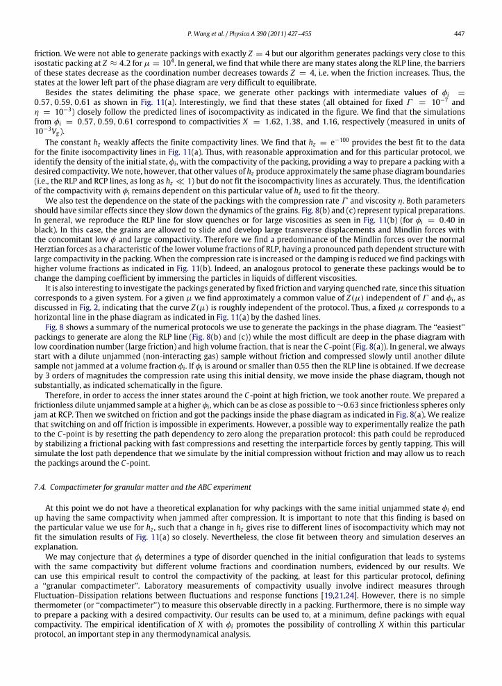
P. Wang et al. / Physica A 390 (2011) 427–455 447
friction. We were not able to generate packings with exactly Z = 4 but our algorithm generates packings very close to thisisostatic packing at Z ≈ 4.2 forµ = 104. In general, we find that while there are many states along the RLP line, the barriersof these states decrease as the coordination number decreases towards Z = 4, i.e. when the friction increases. Thus, thestates at the lower left part of the phase diagram are very difficult to equilibrate.
Besides the states delimiting the phase space, we generate other packings with intermediate values of φi =
0.57, 0.59, 0.61 as shown in Fig. 11(a). Interestingly, we find that these states (all obtained for fixed Γ = 10−7 andη = 10−3) closely follow the predicted lines of isocompactivity as indicated in the figure. We find that the simulationsfrom φi = 0.57, 0.59, 0.61 correspond to compactivities X = 1.62, 1.38, and 1.16, respectively (measured in units of10−3Vg ).
The constant hz weakly affects the finite compactivity lines. We find that hz = e−100 provides the best fit to the datafor the finite isocompactivity lines in Fig. 11(a). Thus, with reasonable approximation and for this particular protocol, weidentify the density of the initial state, φi, with the compactivity of the packing, providing a way to prepare a packing with adesired compactivity.We note, however, that other values of hz produce approximately the same phase diagram boundaries(i.e., the RLP and RCP lines, as long as hz ≪ 1) but do not fit the isocompactivity lines as accurately. Thus, the identificationof the compactivity with φi remains dependent on this particular value of hz used to fit the theory.
We also test the dependence on the state of the packings with the compression rate Γ and viscosity η. Both parametersshould have similar effects since they slow down the dynamics of the grains. Fig. 8(b) and (c) represent typical preparations.In general, we reproduce the RLP line for slow quenches or for large viscosities as seen in Fig. 11(b) (for φi = 0.40 inblack). In this case, the grains are allowed to slide and develop large transverse displacements and Mindlin forces withthe concomitant low φ and large compactivity. Therefore we find a predominance of the Mindlin forces over the normalHerztian forces as a characteristic of the lower volume fractions of RLP, having a pronounced path dependent structure withlarge compactivity in the packing. When the compression rate is increased or the damping is reduced we find packings withhigher volume fractions as indicated in Fig. 11(b). Indeed, an analogous protocol to generate these packings would be tochange the damping coefficient by immersing the particles in liquids of different viscosities.
It is also interesting to investigate the packings generated by fixed friction and varying quenched rate, since this situationcorresponds to a given system. For a given µ we find approximately a common value of Z(µ) independent of Γ and φi, asdiscussed in Fig. 2, indicating that the curve Z(µ) is roughly independent of the protocol. Thus, a fixed µ corresponds to ahorizontal line in the phase diagram as indicated in Fig. 11(a) by the dashed lines.
Fig. 8 shows a summary of the numerical protocols we use to generate the packings in the phase diagram. The ‘‘easiest’’packings to generate are along the RLP line (Fig. 8(b) and (c)) while the most difficult are deep in the phase diagram withlow coordination number (large friction) and high volume fraction, that is near the C-point (Fig. 8(a)). In general, we alwaysstart with a dilute unjammed (non-interacting gas) sample without friction and compressed slowly until another dilutesample not jammed at a volume fraction φi. If φi is around or smaller than 0.55 then the RLP line is obtained. If we decreaseby 3 orders of magnitudes the compression rate using this initial density, we move inside the phase diagram, though notsubstantially, as indicated schematically in the figure.
Therefore, in order to access the inner states around the C-point at high friction, we took another route. We prepared africtionless dilute unjammed sample at a higher φi, which can be as close as possible to∼0.63 since frictionless spheres onlyjam at RCP. Then we switched on friction and got the packings inside the phase diagram as indicated in Fig. 8(a). We realizethat switching on and off friction is impossible in experiments. However, a possible way to experimentally realize the pathto the C-point is by resetting the path dependency to zero along the preparation protocol: this path could be reproducedby stabilizing a frictional packing with fast compressions and resetting the interparticle forces by gently tapping. This willsimulate the lost path dependence that we simulate by the initial compression without friction and may allow us to reachthe packings around the C-point.
7.4. Compactimeter for granular matter and the ABC experiment
At this point we do not have a theoretical explanation for why packings with the same initial unjammed state φi endup having the same compactivity when jammed after compression. It is important to note that this finding is based onthe particular value we use for hz , such that a change in hz gives rise to different lines of isocompactivity which may notfit the simulation results of Fig. 11(a) so closely. Nevertheless, the close fit between theory and simulation deserves anexplanation.
We may conjecture that φi determines a type of disorder quenched in the initial configuration that leads to systemswith the same compactivity but different volume fractions and coordination numbers, evidenced by our results. Wecan use this empirical result to control the compactivity of the packing, at least for this particular protocol, defininga ‘‘granular compactimeter’’. Laboratory measurements of compactivity usually involve indirect measures throughFluctuation–Dissipation relations between fluctuations and response functions [19,21,24]. However, there is no simplethermometer (or ‘‘compactimeter’’) to measure this observable directly in a packing. Furthermore, there is no simple wayto prepare a packing with a desired compactivity. Our results can be used to, at a minimum, define packings with equalcompactivity. The empirical identification of X with φi promotes the possibility of controlling X within this particularprotocol, an important step in any thermodynamical analysis.

448 P. Wang et al. / Physica A 390 (2011) 427–455
Fig. 12. Measuring the temperature of sand. Pictorial representation.
The advance of a granular thermodynamics crucially depends on the invention of a thermometer that can easily measurethe compactivity, as in Fig. 12. A zero-th law of thermodynamics presents serious challenges in granular materials sincethere is no straightforward way to define a compactivity bath or reservoir.
The present theory predicts the dependence of the volume fraction, φ(X), on the compactivity, allowing for thedevelopment of a compactimeter. Such a device consists of a known granular medium, having a given µ and, therefore,a given coordination number. The compactimeter is inserted in a granular system and both system and compactimeter aregently shaken to allow for equilibration at a common compactivity (the compactimeter has a flexible membrane that allowsvolume transfer between both systems in contact). The volume of the grain in the compactimeter will adjust accordinglyand the compactivity can be read directly from the scale attached to it through the equation of state, X(φ), provided by thetheory.
The foundation of the above compactimeter relies on the validity of a zero-th law for granular thermodynamics thatdetermines the equilibration at a given compactivity of a system. Two systems in contact shouldmechanically equilibrate atthe same compactivity. A recent experiment [70] found a materials-independent relationship between the average volumefraction and its fluctuations in two equilibrated granular subsystems, which gives support to the zero-th law. Further testof the zero-th law is difficult to facilitate without theoretical guidance. Thus, it will be useful to perform the following test,either numerically or experimentally to test not only the idea of equilibration but also the possibility to describe granularmatter under the V -ensemble. Such a test has been labeled the ABC experiment as proposed by Edwards [47], which is nowpossible to perform using the phase diagram.
Two packings are numerically prepared at points A and B in Fig. 13 for differentµ, µA < µB. The systems are equilibratedat different compactivities XA < XB by using different φi. They are then put into contact through a flexible membrane (orby simply putting the particles at the surface in contact) and allowed to mechanically equilibrate by gently shaking thesystem. Numerically, this can be simulated with the same compression methods as explained in Section 7. The total volumeis kept fixed and the volumes of the subsystems should change accordingly, V = VA + VB. If the AB system equilibrates atthe same compactivity, then it will follow the trajectory depicted in Fig. 13 towards the state C of equilibration along theisocompactivity line. There is no need to measure the compactivity of the final packing. Just measuring the final volumes VAand VB (or their volume fractions) will suffice. This will provide an important test for the V -ensemble and compactivity todescribe jammed matter, as well as the validity of the phase diagram.
Another intriguing possibility would be to mix a frictionless A packing at the J-point with an infinite friction B packingat the L-point, which can be achieved numerically. This AB system would provide the maximum difference between theisolated packings, allowing study of the zero-th law with more accuracy. According to theory, the frictionless packing isindependent of X . Therefore, it should remain at the J-point. The µ → ∞ packing should, in principle, equilibrate at anyX or volume fraction along the G-line. Most probably, it would stay put at the L-point since the A and B packings are joinedby the isocompactivity X → ∞ line already. In any case, the resulting AB packing should fall inside the phase diagram ifthe theory is correct. If it does not equilibrate (falling outside the phase diagram, we note that the two packings are at theborderline), it could indicate the breakdown of the approach. Two conclusions could be reached from the failure of such atest. Either the V -ensemble is wrong or the approximations of the V -ensemble theory are not correct. If the latter, moresophisticated theories should be developed. If the former case occurs, then a different ensemble will have to be consideredbeyond isostaticity.
7.5. Microscopic states versus mesoscopic states
The notion that RCP arises for X = 0, implying that there are no fluctuations at RCP, deserves some discussion.Furthermore, it is important to discuss the implications of the related coincidence of RCP and RLP at the frictionless point.

P. Wang et al. / Physica A 390 (2011) 427–455 449
Z
Fig. 13. Sketch depicting a possible ABC experiment to test the zero-th law of granular thermodynamics and the validity of the phase diagram for finitecompactivities. For intermediate frictions, the A and B systems should follow the arrows to C when put into contact and allow interchange of volume bygently shaking.
That is, the fact that for frictionless particles there is a unique state of jamming and therefore the compactivity is irrelevantwhen µ = 0.
First of all, we need to emphasize that these results should be interpreted at the mesoscopic level. Thus, there is onemesoscopic state at RCP and only the mesoscopic entropy vanishes at this point. These results provides an unambiguousinterpretation of RCP only at the meso level. As discussed above, for a single mesoscopic state, there are many microscopicstates which average out in the calculation of the average free volume function w(z) which is used in the partition functionEq. (19) (see also Jamming I [49]). Therefore, we expect that these microscopic states will contribute to the entropy of RCP(see Jamming III [51] for a discussion) as well as giving rise to other states perhaps with different volume fraction. Belowwe elaborate on the existence of microscopic and mesoscopic packing states. This point is better discussed in terms of thevolume landscape of Fig. 5: all the jammed states are degenerated around themesoscopic ground statewith the coordinationnumber z = 6. These states have slightly different volume fractions, leading to microscopic fluctuations which are coarse-grained in the mesoscopic theory.
The existence of microscopic states neglected at the mesoscopic level raises an interesting analogy with recent workof Zamponi and Parisi [38] where the jammed states are considered as infinite pressure glassy states obtained after a fastcompression from a liquid state at finite temperature. They propose that a range of different volume fractions of jammingcan be achieved according to the initial state fromwhere the quench is started, with themaximumpossible jammed densityobtained when the initial density is the Kauzmann point of the ideal glass. In their representation (see Fig. 4 in Ref. [38])a range of initial densities in the liquid phase ϕ ∈ [ϕd, ϕK ], where ϕd is the density where many metastable states firstappear in the liquid phase as suggested by mean field model picture of the glass transition, and ϕK is the Kauzmann densityof the ideal glass transition, gives rise to a final density of jamming, ϕj(ϕ), obtained after a fast quench from ϕ. Two limitingdensities of jamming are predicted: theminimumatϕj(ϕd) = ϕth and themaximumvolume fraction obtained after a quenchfrom the Kauzmann point, ϕj(ϕK ) = ϕ0.
This situation could be interpreted in term of neglecting themicroscopic states in our theory. It is also a questionwhetherthe states at infinite pressure obtained using fast quenches from a liquid state ‘‘a la Zamponi’’ are equivalent to the jammedstate obtained in our approach for soft spheres. Our volume ensemble approachmight differ from the energy/force ensembleused in the work of Zamponi–Parisi. Further investigations are required to reveal the possible differences.
7.6. Geometrical versus mechanical coordination number: measuring the behavior of quasiparticles
In Section 7.3 we have tested the predictions of the theory. In this section we attempt to test some of the assumptionsof the theory, especially those related to the quasiparticles of w(z) and the bounds in z and its distribution. A quasiparticleis a mathematical entity that is, in principle, impossible to isolate from the structure of a real packing prepared either withMD computer simulations or experiments, rendering the measurement of their properties from real packings difficult. Thisis because real packings already contain the ensemble average, and we cannot dissociate the ensemble, with the Boltzmanndistribution of states, compactivity and density of states, from the isolated statistics of a quasiparticle.
Quasiparticles can be tested by preparing random packings with prescribed geometrical coordination number. However,below, we argue that we may obtain approximate properties from real packings in the limit X → ∞ and hz → 0 basedon the following observations. First, when X → ∞ the Boltzmann factor is one, and the average in the partition function isflat over the configurations up to the density of states. Furthermore, the density of states is found to be a very fast decayingfunction of z. These two results imply that along the RLP line of real packings (either numerical or experimental) we can

450 P. Wang et al. / Physica A 390 (2011) 427–455
Fig. 14. gz(1r) of packings with various friction coefficients µ along the RCP line. We set 2R = 1.
obtain fully random packings which could reveal the properties of the quasiparticles. Under this approximationwe can thentest some of the approximations of the theory. However, the conclusions from this section remain approximate.
We have proposed that the bounds of the geometrical coordination number are Z ≤ z ≤ 6 and below we test thesebounds.We find numerically that the quasiparticle size is of the order of two particle diameters. Once z is averaged over thisrange, we find that z ranges approximately between (Z, 6). In fact, we find evenmore narrow distribution than theoreticallyexpected. This is due to the fact that we define z without the microscopic fluctuations but including the mesoscopicfluctuations. Once we average over its neighbors, we not only remove the microscopic fluctuations but also, partially, themesoscopic ones. In the limiting case of no mesoscopic fluctuations, when X = 0 along the RCP line, we find a very narrowdistribution at z ≈ 6 for any value of Z and µ, after averaging z over a mesoscopic region of two particle diameters. Thedistribution is even narrower when z is coarse-grained over a region of four particle diameters.
The X-ray tomography experiments of Aste [45] (Fig. 6(a)) reveal the trend predicted by Eq. (7) between the inverse ofthe Voronoi volume and the number of neighbors of a set of Voronoi cells with similar volumes. However, it is evident fromthe figure that such number of neighbors is spanning a range of values between ∼4 and ∼10. The reason why the Aste’sgroup [45] found a wider range of z is possibly due to the fact they did not consider a range of coarse-graining.
A question arises as how to identify the geometrical from the mechanical coordination number, even numerically. Adetailed discussion of this topic appears in Ref. [71]. Below we summarize the results. Strictly speaking, this distinctionis not possible to materialize in real packings. Again, we need to generate random packings from a geometrical point ofview, without resorting to forces, and then study their distribution in real packings where forces are taken into account.Nevertheless, we follow the following approximate scheme to try to obtain information of the quasiparticles from realpackings.
Even in numerical simulations, there is always a round off error associated to measurements. Thus, two particles thatmay not be in contact (giving rise to a zero force) may be close enough to be considered as contributing to the geometricalcoordination. Indeed, it is known that g(r) has a singularity [72], g(r) ∼ (r−0.5)−0.5, implying that there aremany particlesalmost touching. Following this consideration, we introduce a modified radial distribution function (RDF) gz(r) in order toapproximately identify z and Z from real packings:
gz(r) =1N
R2
r2
N−i
N−j=i
Θ
rij
r − R− 1
Θ
r + Rrij
− 1
, r > R (30)
where R is the radius of particle, N is the number of particles, rij is the distance of two particle’s centers, rij = |ri − rj|, and Θ
is the Heaviside step function. The RDF describes the average value of the number of grains in contact with a virtual particleof radius r , and the factor of R2/r2 is the ratio of a real sphere’s area and the virtual one’s.
gz(r) measures the number of balls with their volume intersecting the surface of a sphere of radius r measured fromthe center of a given ball. When r = R in (30) we obtain the mechanical coordination number while the geometricalone is obtained for a small value 1r =
r−R2R = 0 for which we distinctly find a signature from computer simulations,
unambiguously defining it at 1r = 0.04.Figs. 14 and 15 plot the gz(1r) of packings with various friction coefficients µ on the isostatic plane along the RCP and
RLP lines respectively. Following the definition of Eq. (30), gz , with 1r = 0, should be directly equal to the mechanicalcoordination number, Z , and should range from 4 to 6 along both RCP and RLP (if hz ≪ 1) lines which is confirmed by ournumerical simulations in Figs. 14 and 15, respectively.

P. Wang et al. / Physica A 390 (2011) 427–455 451
Fig. 15. gz(1r) of packings with various friction coefficients µ along the RLP line.
Furthermore, as shown in the figures, we find that gz(1r) along the RCP line increases slightly as 1r increases, andfinally reaches the same value of gz at 1r = 0.04 as shown in Fig. 14. We identify the geometrical coordination numberas z = gz(0.04) under the accuracy of the simulations. Therefore, we conclude that all RCP states have approximately thesame geometrical coordination number, z ≈ 6, in agreement with the theory. In terms of the volume landscape of Fig. 5,the states along the RCP line are ground states with different friction at X = 0. Thus they should all have z = 6. We noticethat gz(1r = 0.04) = 6.65 > 6, which may result, firstly, from the approximate nature of our measurements of z fromreal packings since we are not measuring the quasiparticles directly, and, secondly, from the increasing of the coordinationnumber slightly away from the critical point as the local volume fraction φ increases slightly as Z − Zc ∼ (φ − φc)
β . Wenote that Z is also slightly increased from the isostatic point.
Along the RLP line, Fig. 15, we find that the geometrical coordination number as extracted from gz(0.04) is very close tothe mechanical one. Since the RLP line is at X → ∞ and hz ≪ 1, all the states along RLP have z ≈ Z as we move along theline varying the friction coefficient. Thus, the numerical results confirm the theory, and further confirm that the value of hzis very small.
Next, we study the coarse-grained coordination number ⟨z⟩l as defined as
⟨z⟩l =1Nl
R2
r2
Nl−i
Nl−j=i
Θ
rij
r − R− 1
Θ
r + Rrij
− 1
, r > R (31)
where Nl is the number of the particles inside a coarse-grained spherical range with a radius of l. Figs. 16 and 17 plot the PDFof ⟨z⟩l for all the packings along the RCP and RLP lines, respectively. The distributions show a narrow shape, and the averagevalue gives the value of gz(r), i.e.,
⟨z⟩l = gz(r). (32)
We find that all the P(⟨z⟩l) along the RCP line coincide at 1r = 0.04 as shown in Fig. 16(b) and (c), demonstrating thatall the states have approximately the same average value of z (as discussed above), as well as the same distribution. Thedistribution gets narrower as the coarse-graining parameter l increases from l = 2 to l = 4 as shown in Fig. 16(c). On theother hand Z changes as the friction changes following the isostatic condition, as seen in Fig. 16(a). This in good agreementwith the theory.
Along the RLP line, the situation is analogous. As discussed above, z ≈ Z . This is clearly demonstrated in Fig. 17(b)which should be compared with the analogous Fig. 16(b) for the RCP line. Fig. 17(a) also shows how Z changes with frictionin the same way as in Fig. 16(a). More importantly, we find that the bounds of ⟨z⟩l are well approximated between thebounds proposed by the theory (Z, 6). The slight shift towards higher coordinations observed in Fig. 17(b) is due to theapproximate nature of our measurements from real packings and the small increment in volume fraction from the criticalpoint of jamming, as discussed above. Overall, we conclude that along the RCP line, all states have z ≈ 6, with Z changingfrom 6 to 4 as friction is increased. On the other hand, along the RLP line, we find that z ≈ Z . These two results confirm thetheory very well. Fig. 18 summarizes all these finding indicating the ranges of z and Z along the iso-X lines of RCP and RLP,the iso-z vertical lines, and the iso-Z horizontal lines in the phase diagram.

452 P. Wang et al. / Physica A 390 (2011) 427–455
a
b c
Fig. 16. PDF of the coarse-grained coordination number ⟨z⟩l for packings with various friction coefficients µ along the RCP line. (a) 1r = 0 and l = 2;(b) 1r = 0.04 and l = 2; (c) 1r = 0.04 and l = 4.
a
b
Fig. 17. PDF of the coarse-grained coordination number ⟨z⟩l for packings with various friction coefficients µ along the RLP line. (a) 1r = 0 and l = 2;(b) 1r = 0.04 and l = 2.
8. Outlook
We have presented several results in the disordered sphere packing problem and here will discuss their significance.We start with the results that we believe are more robust and may survive higher scrutiny, and follow with the results thatrequire further study plus a discussion on how to improve the theory.
The final result of the phase diagram, the characterization of RCP andRLP using the compactivity, and the role of friction inthe determination of the limiting packings are interesting results, almost independent of the theory. The distinction betweenthe geometrical and mechanical coordination number is also important, allowing for the implementation of averages in thepartition function. On the mathematical side, the microscopic volume function and the formula obtained for the Voronoicell in Jamming I [49] are important and exact results which are the foundation of all preceding work presented herein.

P. Wang et al. / Physica A 390 (2011) 427–455 453
Fig. 18. Summary of the theoretical findings regarding the range of z and Z along the different iso-z, iso-Z , and iso-X lines and the J, C , and L-points in thephase diagram.
While the predictions Eqs. (24) and (25) of RCP and RLP approximate very well the known values, they are obviouslynot exact expressions, since they are based on several approximations of the statistical theory of volumes. Thus, theimplementation of the mesoscopic volume function and the probability distribution of volumes on which these resultsare based are, perhaps, the points where improvements may be necessary. While the 2
√3
z formula reproduces the averagevolume fraction surprisingly well, it is based on approximations to calculate the probability distribution of volumes, P>(c),as explained in Jamming I [49]. More work is needed to obtain better approximations to such a distribution to capturenot only the mean value of the Voronoi volume but higher moments as well. A full discussion is performed in JammingIV [52]. The present theory shows the way to improve upon Jamming I and obtain an exact formulation of P>(c), at least toa prescribed value of the coordination shell. Such a formulation is presently being developed and is based on a systematicstudy of quasiparticles with fixed geometrical coordination number; it produces good fits of P(W s
i ) for the case of 2d, while3d calculations are under way.
Other approximations that require additional attention are the considerations leading to the density of states g(z). Whilethe main results of RCP and RLP are nearly independent of the particular form of g(z), other quantities such as the entropyand the equations of state for finite nonzero compactivity are more sensitive to it. By a direct measurement of the entropy,g(z) can be calculated and compared to the simple exponential form used in the present study.
Furthermore, we have explicitly removed crystal states from our calculations by considering the upper bound of z = 6.A more general theory is needed then to investigate the transition from the RCP to the FCC as crystals start to form in thesystem. Such a theory will include not only disordered states but also partially crystallized states and would give X = 0 atFCC following the full Edwards partition function, Eq. (5). We investigate this idea in Ref. [69], where we find that RCP canbe interpreted as the ‘‘freezing point’’ in a first-order phase transition between ordered and disordered packing phases.
The distribution of coordination number, assumed to be a delta function, is another approximation to be improved upon.Once again, this may not affect the predicted RCP and RLP but deeper studies require also a distribution of z. A more generalensemble is being considered that predicts the distribution of z in good agreement with the existing data (see JammingIV [52]).
Finally, the extension to study the microstates requires more investigation. The identification of the elementary units asquasiparticles of fixed coordination number is interesting and could eventually lead to more precise solutions of RCP andRLP.
9. Conclusions
In conclusion, using Edwards statistical mechanics we have elucidated some aspects of RLP and RCP in the disorderedspherical packing problem. The numerical results suggest a way to experimentally test the existence of the predictedpackings. By allowing the grains to settle in liquids of varyingdensity, the speedof theparticles canbe varied and a systematicexploration of the jamming phase diagram can be achieved.
Beyond the elucidation of some questions in the sphere packing problem, other problems can now be addressedsystematically from the point of view of what we have learned from the phase diagram. This includes the investigationof the criticality of the jamming transition from frictionless to frictional systems by extending the phase space to (φ, Z, σ ),and generating packings away from the isostatic plane by isotropically compressing the packings generated in the plane ofFig. 4. Previous studies have focused on the frictionless point and on fixed friction. According to our results it is important tosample all the phase space for different friction and compactivities according to the preparation protocols explained above.

454 P. Wang et al. / Physica A 390 (2011) 427–455
log(P)
6
4
RLP RCP
isos
tatic
pla
ne
J point
Jamming
Fig. 19. Sketch depicting a possible extension of the phase diagram of Fig. 4 in the (φ, Z) isostatic plane at the jamming transition to the full phase diagramin the (φ, Z, σ ) space to investigate the criticality of the jamming transition for all packings with any friction coefficient.
Previous results find power law scaling [28,31,27,30] where the stress vanishes as σ ∼ (φ − φc)α . A possible scenario is
depicted in the extended phase diagram of Fig. 19 in the 3-dimensional space (φ, Z, σ ), which could be tested numericallyand experimentally. We note in passing that all the results in the present study refer to the isostatic plane at the jammingtransition σ = 0 or hard sphere limit. We expect that, as we compress packings of soft spheres, different planes of σ =
constant = 0 will be obtained as shown in Fig. 19. These compressed states are described not only by the compactivity Xbut also the angoricity A through the full partition function in the VF ensemble, Eq. (2). Our preliminary results indicatethat there seems to be evidence of criticality as the isostatic plane is approached when σ → 0, although with exponentsdependent on friction as well as the value of the compactivity.
Additional topics to be addressed by means of the presented approach include characterization of jamming in the phasespace of configurations, the problem of elasticity and Green’s function and the study of the pair correlation function g(r),the volume distribution P(W s
i ), Voronoi volume, P(Wvori ), and coordination number P(z), which are within the reach of the
present approach. Other systems under consideration are two-dimensional systems [53], polydisperse systems [54], as wellas the mean field case of infinite dimension. These are interesting cases, since there are many questions debated as to whatis the more dense state in higher dimension. Extensions to other systems such as anisotropic particles are also within thereach of the present approach.
Finally, a complete characterization of the VF-ensemble can now be performed through the measurement of otherquantities as a function of the volume fraction, such as the force distribution P(Fn, Ft), and equations of state through theangoricity in the (φ, Z, σ ) space. Some of these quantities can be obtained analytically from the ensembles allowing forinteresting predictions.
The phase diagram introduced here serves as a beginning to understand how random packings fill space in 3d. Thecomparative advantage of the present approach over extensive work done in the past, is in the classification of all packingsthrough X, Z and φ in the theoretical phase diagram from where these studies could be systematically performed. Thisclassification guides the search for indications of jamming from a systematic point of view, through the exploration of alljammed states from µ = 0 to µ → ∞.
Acknowledgements
This work is supported by the National Science Foundation, CMMTDivision and the Department of Energy, Office of BasicEnergy Sciences, Geosciences Division. We are grateful to B. Brujić and A. Yupanqui for inspirations, C. Briscoe for a criticalreading of the manuscript and the hospitality of UFC, Fortaleza where part of this work was done.
References
[1] T.C. Hales, http://arxiv.org/-abs/math.MG/9811078.[2] A. Thue, Forand. de Skand. Natur. 14 (1892) 352–353.[3] A. Thue, Christinia Vid. Selsk. Skr. 1 (1910) 1–9.[4] J.D. Bernal, J. Mason, Nature 188 (1960) 910;
J.D. Bernal, Nature 185 (1960);J.D. Bernal, Proc. R. Soc. Lond. Ser. A 280 (1964) 299.
[5] Anonymous, Nature 239 (1972) 488.[6] G.D. Scott, D.M. Kilgour, Br. J. Appl. Phys.; J. Phys. D 2 (1969) 863–866;
G.D. Scott, Nature 188 (1960) 908.[7] J.L. Finney, Proc. R. Soc. Lond. Ser. A 319 (1970) 479.

P. Wang et al. / Physica A 390 (2011) 427–455 455
[8] J.D. Berryman, Phys. Rev. A 27 (1983) 1053–1061.[9] G.Y. Onoda, E.G. Liniger, Phys. Rev. Lett. 64 (1990) 2727.
[10] S. Torquato, T.M. Truskett, P.G. Debenedetti, Phys. Rev. Lett. 84 (2000) 2064.[11] A. Coniglio, A. Fierro, H. Hermann, M. Nicodemi (Eds.), Unifying Concepts in Granular Media and Glasses, Elsevier, 2004.[12] R.P. Behringer, J.T. Jenkins (Eds.), Powders & Grains, vol. 97, Balkema, Rotterdam, 1997.[13] S.F. Edwards, R.B.S. Oakeshott, Physica A 157 (1989) 1080–1090.[14] S.F. Edwards, The role of entropy in the specification of a powder, in: A. Mehta (Ed.), Granular Matter: An Interdisciplinary Approach, Springer-Verlag,
New York, 1994, pp. 121–140.[15] S.F. Edwards, Physica A 353 (2005) 114.[16] R. Blumenfeld, S.F. Edwards, Phys. Rev. Lett. 90 (2002) 114303.[17] E. Bertin, O. Dauchot, M. Droz, Phys. Rev. Lett. 96 (2006) 120601.[18] M.P. Ciamarra, A. Coniglio, M. Nicodemi, Phys. Rev. Lett. 97 (2006) 158001.[19] E.R. Nowak, J.B. Knight, E. BenNaim, H.M. Jaeger, S.R. Nagel, Phys. Rev. E 57 (1998) 1971.[20] J. Brujić, P. Wang, D.L. Johnson, O. Sindt, H.A. Makse, Phys. Rev. Lett. 95 (2005) 128001.[21] M. Schröter, D.I. Goldman, H.L. Swinney, Phys. Rev. E 71 (2005) 030301(R).[22] L.F. Cugliandolo, J. Kurchan, L. Peliti, Phys. Rev. E 55 (1997) 3898.[23] A. Barrat, J. Kurchan, V. Loreto, M. Sellitto, Phys. Rev. Lett. 85 (2000) 5034.[24] H.A. Makse, J. Kurchan, Nature 415 (2002) 614.[25] A. Fierro, M. Nicodemi, M. Tarzia, A. de Candia, A. Coniglio, Phys. Rev. E 71 (2005) 061305.[26] A. Liu, S.R. Nagel, Nature 396 (1998) 21–22.[27] H.A. Makse, D.L. Johnson, L.M. Schwartz, Phys. Rev. Lett. 84 (2000) 4160.[28] C.S. O’Hern, S.A. Langer, A.J. Liu, S.R. Nagel, Phys. Rev. Lett. 88 (2002) 075507.[29] C.S. O’Hern, L.E. Silbert, A.J. Liu, S.R. Nagel, Phys. Rev. E 68 (2003) 011306.[30] H. Zhang, H.A. Makse, Phys. Rev. E 72 (2005) 011301.[31] L.E. Silbert, D. Ertas, G.S. Grest, T.C. Halsey, D. Levine, Phys. Rev. E 65 (2002) 031304.[32] V. Trappe, V. Prasad, L. Cipelletti, P.N. Segre, D.A. Weitz, Nature 411 (2001).[33] T. Under, J. Kertesz, D.E. Wolf, Phys. Rev. Lett. 94 (2005) 178001.[34] K. Shundyak, M. van Hecke, W. van Saarloos, Phys. Rev. E 75 (2007) 010301.[35] L.D. Landau, E.M. Lifshitz, Theory of Elasticity, Pergamon, NY, 1970.[36] R.D. Mindlin, Trans. ASME J. Appl. Mech. 71 (1949).[37] J. Brujić, S.F. Edwards, D.V. Grinev, I. Hopkinson, D. Brujić, H.A. Makse, Faraday Discuss. 123 (2003) 207.[38] G. Parisi, F. Zamponi, Rev. Modern Phys. 82 (2010) 789–845.[39] B.D. Lubachevsky, F.H. Stillinger, J. Stat. Phys. 60 (1990) 561.[40] M. Skoge, A. Donev, F.H. Stillinger, S. Torquato, Phys. Rev. E 74 (2006) 041127.[41] F. Krzakala, J. Kurchan, Phys. Rev. E 76 (2007) 021122.[42] P. Philippe, D. Bideau, Europhys. Lett. 60 (2002) 677.[43] S. Henkes, B. Chakraborty, Phys. Rev. Lett. 95 (2005) 198002.[44] R. Blumenfeld, On entropic characterization of granular materials, in: Granular and Complex Materials, in: Lecture Notes in Complex Systems, vol. 8,
2007, pp. 43–53.[45] T. Aste, M. Saadatfar, T.J. Senden, J. Stat. Mech. (2006) P07010.[46] F. Lechenault, F. da Cruz, O. Dauchot, E. Bertin, J. Stat. Mech. (2006) P07009.[47] H.A. Makse, J. Brujić, S.F. Edwards, Statistical mechanics of jammed matter, in: H. Hinrichsen, D.E. Wolf (Eds.), The Physics of Granular Media, Wiley-
VCH, 2004.[48] L.D. Landau, E.M. Lifshitz, Statistical Physics, Pergamon, NY, 1970.[49] C. Song, P. Wang, Y. Jin, H.A. Makse, Physica A 389 (2010) 4497.[50] C. Song, P. Wang, H.A. Makse, Nature 453 (2008) 629.[51] C. Briscoe, C. Song, P. Wang, H.A. Makse, Physica A 389 (2010) 3978.[52] P. Wang, C. Song, Y. Jin, H.A. Makse, e-print. arXiv:0808.2198.[53] S. Meyer, C. Song, Y. Jin, K. Wang, H.A. Makse, Physica A 389 (2010) 5137.[54] M. Danisch, Y. Jin, H.A. Makse, Phys. Rev. E 81 (2010) 051303.[55] J.A. van Meel, B. Charbonneau, A. Fortini, P. Charbonneau, Phy. Rev. E 80 (2009) 061110.[56] R.C. Ball, R. Blumenfeld, Phys. Rev. Lett. 88 (2002) 115505-1.[57] R. Blumenfeld, Eur. Phys. J. B 29 (2005) 261.[58] J. Zhou, S. Long, Q. Wang, Science 312 (2006) 1631.[59] S. Alexander, Phys. Rep. 296 (1998) 65.[60] C.F. Moukarzel, Phys. Rev. Lett. 81 (1998) 1634.[61] S.F. Edwards, D.V. Grinev, Phys. Rev. Lett. 82 (1999) 5397.[62] S. Torquato, F.H. Stillinger, J. Phys. Chem. B 105 (2001) 11849.[63] J. Brujić, C. Song, P. Wang, C. Briscoe, G. Marty, H.A. Makse, Phys. Rev. Lett. 98 (2007) 248001.[64] F.H. Stillinger, Science 267 (1995) 1935–1939.[65] H.A. Makse, N. Gland, D.L. Johnson, L.M. Schwartz, Phys. Rev. Lett. 83 (1999) 5070.[66] H.A. Makse, N. Gland, D.L. Johnson, L.M. Schwartz, Phys. Rev. E 70 (2004) 061302.[67] F. Zamponi, Nature 453 (2008) 606.[68] S. Mukhopadhyay, M.L. Gilchrist, H.A. Makse (in preparation).[69] Y. Jin, H.A. Makse, Physica A 389 (2010) 5362.[70] F. Lechenault, K.E. Daniels, e-print. arXiv:1001.5411.[71] C. Song, P. Wang, H.A. Makse, AIP Conf. Proc. 1227 (2010) 271.[72] A. Donev, et al., Phys. Rev. E 71 (2005) 011105.