A System of Experimental DesignC. F. Jeff Wu

Georgia Institute of Technology

• System has four broad branches :(i) regular orthogonal designs,(ii) nonregular orthogonal designs,(iii) response surface designs,(iv) optimal designs.

• New opportunities in boarder areas.– Interface between (ii) <=> (iii), (iii) <=> (iv).– Space-filling designs.

New materials available in “Experiments: Planning, Analysis and Parameter Design Optimization” by Wu - Hamada (2000)

Regular orthogonal designs ( Fisher, Yates, Finney, …): designs, using minimum aberration criterion

Nonregular orthogonal designs (Plackett-Burman, Rao, Bose): Plackett-Burman designs, orthogonal arrays

(factor screening, projection)

Response surface designs (Box) : fitting a parametric response surface

Optimal designs (Kiefer): optimality driven by specific model/criterion

knkn −− 3 ,2

Fundamental Principles for Factorial Effects

• Effect Hierarchy Principle:– Lower order effects more important than higher order

effects– Effects of same order equally important

• Effect Sparsity Principle: Number of relatively important effects is small

• Effect Heredity Principle: for an interaction to be significant, at least one of its parent factors should be significant

Fractional Factorial DesignsRun 1 2 3 12 13 23 123

1 - - - + + + - 2 - - + + - - + 3 - + - - + - + 4 - + + - - + - 5 + - - - - + + 6 + - + - + - - 7 + + - + - - - 8 + + + + + + +

col “12” = (col 1) × (col2), etc.

• 4 factors: 1, 2, 3, 4 =12 (4 & 12 are said to be aliased)24-1 design: I =124

• 5 factors: 1, 2, 3, 4 =12, 5 =1325-2 design: I =124 =135 = 2345

(defining contrast subgroup)

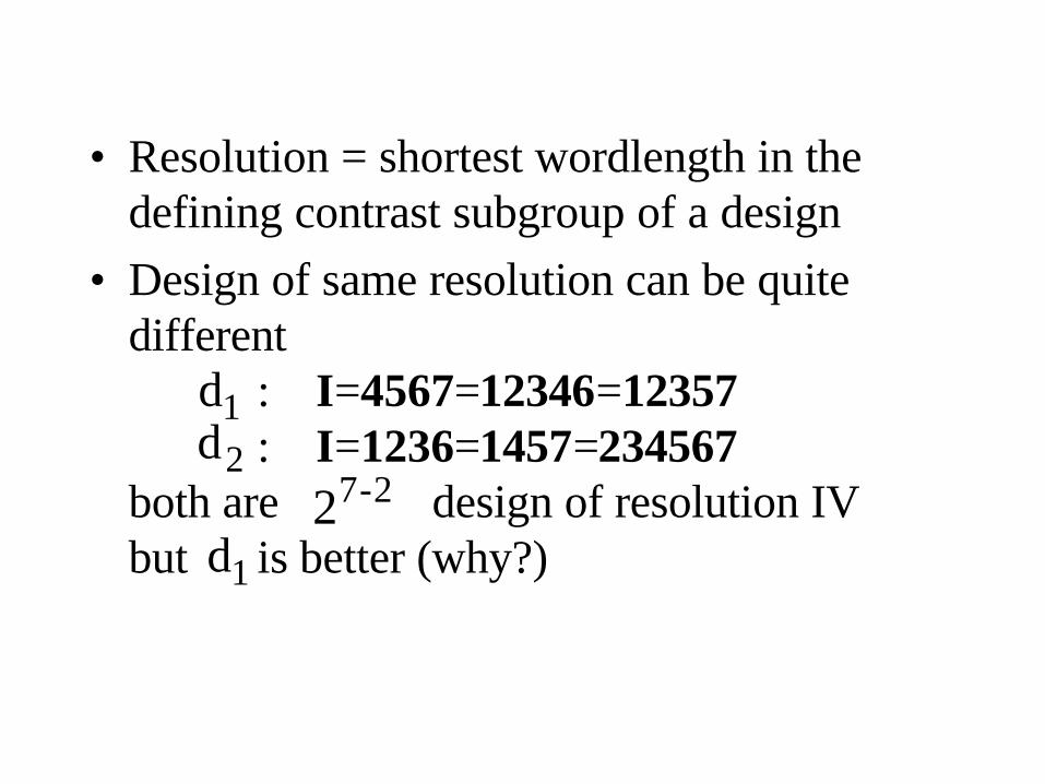
• Resolution = shortest wordlength in the defining contrast subgroup of a design

• Design of same resolution can be quite different

: I=4567=12346=12357: I=1236=1457=234567

both are design of resolution IV but is better (why?)

1d2d

1d272 -

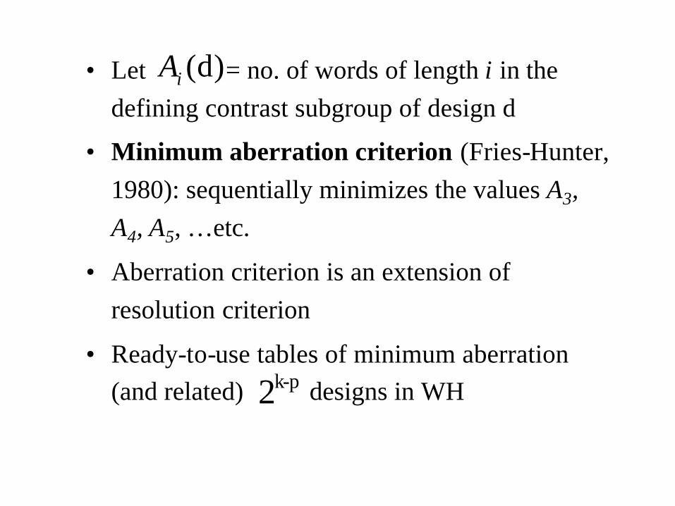
• Let = no. of words of length i in the defining contrast subgroup of design d

• Minimum aberration criterion (Fries-Hunter, 1980): sequentially minimizes the values A3, A4, A5, …etc.

• Aberration criterion is an extension of resolution criterion

• Ready-to-use tables of minimum aberration (and related) designs in WH

)d(iA

pk2 -

Thirty-Two Run Fractional Factorial Designs

Extensions of Minimum Aberration to Designs with Factor Asymmetry

• 2n-k designs in 2q blocks: “treatment defining contrast subgroup”, and “block defining contrast subgroup” are intertwined

• 2n-k parameter designs, control and noise factors(control-by-noise interaction key to robustness):modified effect hierarchy principle: c, n, cn (1st group), cc, ccn, nn (2nd group), etc.

• 2n-k split-plot designs, n1 whole-plot factors, n2split-plot factors: wp effects, wp x sp effects, speffects treated differently, two variance components

Two Types of Fractional Factorial Designs:• Regular ( designs):

columns of the design matrix form a group over a finite field; the interaction between any two columns is among the columns⇒ any two factorial effects are either

orthogonal or fully aliased• Nonregular (mixed-level designs, orthogonal

arrays)some pairs of factorial effects can be partiallyaliased⇒ more complex aliasing pattern

knkn −− 3 ,2

Orthogonal Arrays

• Two columns of a design matrix are orthogonal if all possible level combinations of the two columns appear equally often in the matrix

• An orthogonal array of strength two is an N×m matrix,

in which columns have levels and any two columns are orthogonal

• 2n-k, 3n-k designs are OA’s

)ssOA(N k1 mk

m1 ⋅⋅⋅⋅,

k1 mmm +⋅⋅⋅+= im is

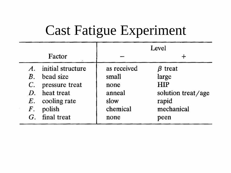
Cast Fatigue Experiment

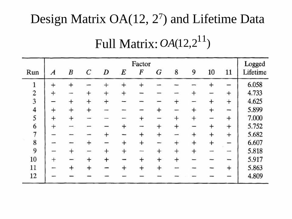
Design Matrix OA(12, 27) and Lifetime Data

Full Matrix: )2,12( 11OA

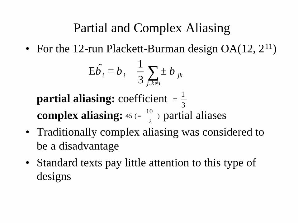
Partial and Complex Aliasing• For the 12-run Plackett-Burman design OA(12, 211)

partial aliasing: coefficient complex aliasing: partial aliases

• Traditionally complex aliasing was considered to be a disadvantage

• Standard texts pay little attention to this type of designs

∑≠

±+=ikj

jkii,3

1 ˆE βββ

31±

)2

10 ( 45

=

Useful Orthogonal Arrays• Collection in WH

• Run Size Economyvs.16-run designs, vs. 27-run designs,

• Flexibility in level combinations

)2,12( 11OA )23,12( 41OA)26,18( 61OA)26,24( 141OA

)2,12( 11OA

)2,20( 19OA)32,18( 71OA

)62,36( 38OA )42,48( 1211OA )52,50( 111OA)32,36( 1211OA

)23,24( 161OA

)32,54( 251OA

)63,36( 37OA

)3,18( 7OA

p-k2 11k8 ≤≤p-k3 7k5 ≤≤

Blood Glucose Experiment

)32,18( 71OA

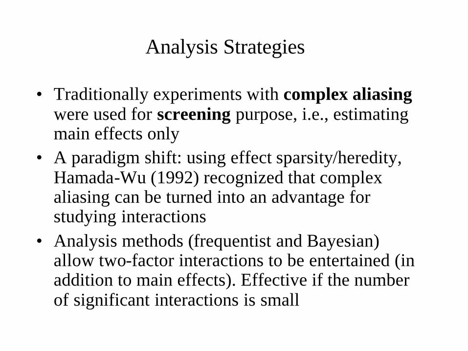
• Traditionally experiments with complex aliasingwere used for screening purpose, i.e., estimating main effects only

• A paradigm shift: using effect sparsity/heredity, Hamada-Wu (1992) recognized that complex aliasing can be turned into an advantage for studying interactions

• Analysis methods (frequentist and Bayesian) allow two-factor interactions to be entertained (in addition to main effects). Effective if the number of significant interactions is small

Analysis Strategies

• Cast Fatigue Experiment:Main effect analysis: F (R2=0.45)

F, D (R2=0.59)HW analysis: F, FG (R2=0.89)

F, FG, D (R2=0.92)

• Blood Glucose Experiment:Main effect analysis: Eq, Fq (R2=0.36)HW analysis: Bl, (BH)lq, (BH)qq (R2=0.89)

Bayesian analysis also identifies Bl, (BH)ll, (BH)lq, (BH)qq as having the highest posterior model probability

Examples

• Success in the HW analysis strategy led to research on the hidden projection properties of nonregular designs. Commonly used arrays like OA(12, 211), OA(18, 37), OA(36, 211312) have desirable projection properties (i.e., for 4 - 8 factors, a number of interactions can be estimated with good efficiency)

• This is achieved without adding new runs• It has also inspired a new approach to response

surface methodologyFurther Analysis

Further Analysis

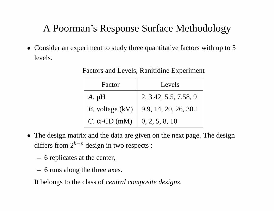
A Poorman’s Response Surface Methodology

• Consider an experiment to study three quantitative factorswith up to 5

levels.

Factors and Levels, Ranitidine Experiment

Factor Levels

A. pH 2, 3.42, 5.5, 7.58, 9

B. voltage (kV) 9.9, 14, 20, 26, 30.1

C. α-CD (mM) 0, 2, 5, 8, 10

• The design matrix and the data are given on the next page. The design

differs from 2k−p design in two respects :

– 6 replicates at the center,

– 6 runs along the three axes.

It belongs to the class ofcentral composite designs.

Ranitidine Experiment

Design Matrix and Response Data

Factor

Run A B C CEF ln CEF

1 −1 −1 −1 17.293 2.850

2 1 −1 −1 45.488 3.817

3 −1 1 −1 10.311 2.333

4 1 1 −1 11757.084 9.372

5 −1 −1 1 16.942 2.830

6 1 −1 1 25.400 3.235

7 −1 1 1 31697.199 10.364

8 1 1 1 12039.201 9.396

9 0 0 −1.67 7.474 2.011

10 0 0 1.67 6.312 1.842

11 0 −1.68 0 11.145 2.411

12 0 1.68 0 6.664 1.897

13 −1.68 0 0 16548.749 9.714

14 1.68 0 0 26351.811 10.179

15 0 0 0 9.854 2.288

16 0 0 0 9.606 2.262

17 0 0 0 8.863 2.182

18 0 0 0 8.783 2.173

19 0 0 0 8.013 2.081

20 0 0 0 8.059 2.087

Central Composite DesignsA simple CCD is shown graphically below. It has three parts(1) cube ( or corner) points, (2) axial (or star) points, (3) center points.

A Central Composite Design in Three Dimensions (cube point (dot), star point(cross), center point (circle))

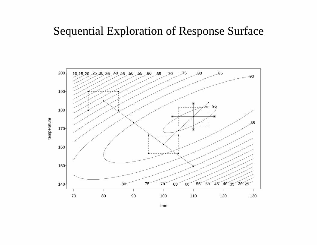
Sequential Exploration of Response Surface

time

tem

pera

ture

10 15 20 25

25

30

30

35

35

40

40

45

45

50

50

55

55

60

60

65

65

70

70

75

75

80

80

85

8590

95•

•

•

•

•

•

•

•

70 80 90 100 110 120 130

140

150

160

170

180

190

200

• •

• •

•

•

•

•

An Alternative to Standard Response Surface Methodology

• Standard RSM employs a 2-stage experimentation strategy; this can be time consuming and expensive.

• S. W. Cheng - Wu (2001) proposed a new strategy to perform factor screening (1st order model) and response surface exploration (2nd order model) on the same experiment using one design, based on new optimality criteria called projection -aberration

Optimal Designs• D-,G-,I-optimality based on a single model,

performance not guaranteed over a variety of models. Performance is highly model-dependent.

• Exact optimality more interesting than approximate (continuous) optimality. Algorithms make more impact than theory; generally applicable to any models.

• Bigger impact when used in conjunction with or as a supplement to a combinatorial or reasonably uniform design (irregular design, follow-up experiment, sequential designs).

• Generally useful as a benchmark.

Space-Filling Designs

• Latin Hypercube insd (McKay, Beckman, Conover, 1979):one-dimensional

balance for each of thed dimensions withs levels. Various extensions

available: OA-based LHS (Tang, 1993) achieves 2- or higher-dimensional

balance by combining LHS and OA.

• Uniform designs (Fang): based on wrapping around a sequencein high

dimensions using number-theoretic justifications. More generally,good

lattice points: work by Niederreiter etc.

• Design criteria and modeling are drasticallydifferent from all the previous

approaches: space-filling, minimax or maximin distance; use of

semi-parametric modeling or Gaussian process modeling that allows highly

nonlinear fitting.

25 points of a Latin hypercube sample

25 points of a randomly centered randomized orthogonal array. For any two variables, there is one point in each reference square.

25 points of an OA-based Latin hypercube sample

Innovations in Bayesian Analysis for Designed Experiments

• Choice of priors reflects the three principles (hierarchy, sparsity, heredity)

• Model search strategy depends on nature of design (much easier for regular designs; not so for nonregular designs); strategy should exploit the effect aliasing pattern

• Convenient for computer experiments.

A Summary of Layout Techniques

A flexible strategy for selecting a suitable design from among

(i) 2k−p designs : 8, 16, 32, 64, 128-run designs.

(ii) 3k−p designs : 9, 27, 81-run designs (optimal selection of factorcolumns by

minimum aberration criterion).

(iii) Plackett-Burman designs :OA(12,211), OA(20,219),...

(iv) Mixed-level designs :OA(8,4124),OA(16,4m2n) (derived from 2k−p

designs),OA(18,2137), OA(36,211312), OA(12,3124), OA(24,31216), ...

(allowing main effects and a flexible choice of interactionsto be estimated;

hidden-projection property).

(v) Central Composite designs.

(vi) Optimal Designs (SAS/QC).

(vii) Space-filling designs (Latin hypercube designs).