jorge cardoso - observing and controlling...
TRANSCRIPT

Master’s Degree in Informatics EngineeringFinal Dissertation
Observing and Controlling Performancein Microservices
Author:André Pascoal Bento
Supervisor:Prof. Filipe João Boavida Mendonça Machado Araújo
Co-Supervisor:Prof. António Jorge Silva Cardoso
July 2019

This page is intentionally left blank.
Abstract
Microservice based software architecture are growing in us-age and one type of data generated to keep history of the workperformed by this kind of systems is called tracing data. Trac-ing can be used to help Development and Operations (DevOps)perceive problems such as latency and request work-flow intheir systems. Diving into this data is difficult due to its com-plexity, plethora of information and lack of tools. Hence, itgets hard for DevOps to analyse the system behaviour in orderto find faulty services using tracing data. The most commonand general tools existing nowadays for this kind of data, areaiming only for a more human-readable data visualisation torelieve the effort of the DevOps when searching for issues intheir systems. However, these tools do not provide good waysto filter this kind of data neither perform any kind of tracingdata analysis and therefore, they do not automate the task ofsearching for any issue presented in the system, which standsfor a big problem because they rely in the system adminis-trators to do it manually. In this thesis is present a possiblesolution for this problem, capable of use tracing data to extractmetrics of the services dependency graph, namely the numberof incoming and outgoing calls in each service and their corre-sponding average response time, with the purpose of detectingany faulty service presented in the system and identifying themin a specific time-frame. Also, a possible solution for qualitytracing analysis is covered checking for quality of tracing struc-ture against OpenTracing specification and checking time cov-erage of tracing for specific services. Regarding the approachto solve the presented problem, we have relied in the imple-mentation of some prototype tools to process tracing data andperformed experiments using the metrics extracted from trac-ing data provided by Huawei. With this proposed solution, weexpect that solutions for tracing data analysis start to appearand be integrated in tools that exist nowadays for distributedtracing systems.
Keywords
Microservices, Cloud Computing, Observability, Monitor-ing, Tracing.
i

This page is intentionally left blank.
Resumo
A arquitetura de software baseada em micro-serviços estáa crescer em uso e um dos tipos de dados gerados para mantero histórico do trabalho executado por este tipo de sistemas édenominado de tracing. Mergulhar nestes dados é díficil de-vido à sua complexidade, abundância e falta de ferramentas.Consequentemente, é díficil para os DevOps de analisarem ocomportamento dos sistemas e encontrar serviços defeituososusando tracing. Hoje em dia, as ferramentas mais gerais e co-muns que existem para processar este tipo de dados, visamapenas apresentar a informação de uma forma mais clara, ali-viando assim o esforço dos DevOps ao pesquisar por proble-mas existentes nos sistemas. No entanto, estas ferramentas nãofornecem bons filtros para este tipo de dados, nem formas deexecutar análises dos dados e, assim sendo, não automatizam oprocesso de procura por problemas presentes no sistema, o quegera um grande problema porque recaem nos utilizadores parao fazer manualmente. Nesta tese é apresentada uma possivelsolução para este problema, capaz de utilizar dados de tracingpara extrair metricas do grafo de dependências dos serviços,nomeadamente o número de chamadas de entrada e saída emcada serviço e os tempos de resposta coorepondentes, com opropósito de detectar qualquer serviço defeituoso presente nosistema e identificar as falhas em espaços temporais especificos.Além disto, é apresentada também uma possivel solução parauma análise da qualidade do tracing com foco em verificar aqualidade da estrutura do tracing face à especificação do Open-Tracing e a cobertura do tracing a nível temporal para serviçosespecificos. A abordagem que seguimos para resolver o prob-lema apresentado foi implementar ferramentas protótipo paraprocessar dados de tracing de modo a executar experiênciascom as métricas extraidas do tracing fornecido pela Huawei.Com esta proposta de solução, esperamos que soluções paraprocessar e analisar tracing comecem a surgir e a serem in-tegradas em ferramentas de sistemas distribuidos.
Palavras-Chave
Micro-serviços, Computação na nuvem, Observabilidade,Monitorização, Tracing.
iii

This page is intentionally left blank.

Acknowledgements
This work would not be possible to be accomplished withouteffort, help and support from my family, fellows and colleagues.Thus, in this section I would like to give my sincere thanks toall of them.
Starting by giving thanks to my mother and to my wholefamily, who have supported me through this entire and longjourney, and who always gave and will always give me someof the most important and beautiful things in life, love andfriendship.
In second place, I would like to thank all people that wereinvolved directly in this project. To my supervisor, ProfessorFilipe Araújo, who contributed with his vast wisdom and ex-perience, to my co-supervisor, Professor Jorge Cardoso, whocontributed with is vision and guidance about the main roadwe should take and to Engineer Jaime Correia, who “breathes”these kind of topics through him and helped a lot with is enor-mous knowledge and enthusiasm.
In third place, I would like to thank Department of Infor-matics Engineering and the Centre for Informatics and Sys-tems, both from the University of Coimbra, for allowing andprovide the resources and facilities to to be carried out thisproject.
In fourth place, to the Foundation for Science and Tech-nology (FCT), for financing this project facilitating its accom-plishment, to Huawei, for providing tracing data, core for thiswhole research, and to Portugal National Distributed Com-puting Infrastructure (INCD) for providing hardware to runexperiments.
And finally, my sincere thanks to everyone that I have notmentioned and contributed to everything that I am today.
v

This page is intentionally left blank.

Contents
1 Introduction 11.1 Context . . . . . . . . . . . . . . . . . . . . . . . . . . . . . . . . . . . . . . 11.2 Motivation . . . . . . . . . . . . . . . . . . . . . . . . . . . . . . . . . . . . 21.3 Goals . . . . . . . . . . . . . . . . . . . . . . . . . . . . . . . . . . . . . . . 21.4 Work Plan . . . . . . . . . . . . . . . . . . . . . . . . . . . . . . . . . . . . . 31.5 Research Contributions . . . . . . . . . . . . . . . . . . . . . . . . . . . . . 71.6 Document Structure . . . . . . . . . . . . . . . . . . . . . . . . . . . . . . . 7
2 State of the Art 92.1 Concepts . . . . . . . . . . . . . . . . . . . . . . . . . . . . . . . . . . . . . 9
2.1.1 Microservices . . . . . . . . . . . . . . . . . . . . . . . . . . . . . . . 92.1.2 Observability and Controlling Performance . . . . . . . . . . . . . . 112.1.3 Distributed Tracing . . . . . . . . . . . . . . . . . . . . . . . . . . . 112.1.4 Graphs . . . . . . . . . . . . . . . . . . . . . . . . . . . . . . . . . . 142.1.5 Time-Series . . . . . . . . . . . . . . . . . . . . . . . . . . . . . . . . 15
2.2 Technologies . . . . . . . . . . . . . . . . . . . . . . . . . . . . . . . . . . . . 172.2.1 Distributed Tracing Tools . . . . . . . . . . . . . . . . . . . . . . . . 172.2.2 Graph Manipulation and Processing Tools . . . . . . . . . . . . . . . 182.2.3 Graph Database Tools . . . . . . . . . . . . . . . . . . . . . . . . . . 202.2.4 Time-Series Database Tools . . . . . . . . . . . . . . . . . . . . . . . 22
2.3 Related Work . . . . . . . . . . . . . . . . . . . . . . . . . . . . . . . . . . . 242.3.1 Mastering AIOps . . . . . . . . . . . . . . . . . . . . . . . . . . . . . 242.3.2 Anomaly Detection using Zipkin Tracing Data . . . . . . . . . . . . 242.3.3 Analysing distributed trace data . . . . . . . . . . . . . . . . . . . . 252.3.4 Research possible directions . . . . . . . . . . . . . . . . . . . . . . . 26
3 Research Objectives and Approach 273.1 Research Objectives . . . . . . . . . . . . . . . . . . . . . . . . . . . . . . . 273.2 Research Questions . . . . . . . . . . . . . . . . . . . . . . . . . . . . . . . . 28
4 Proposed Solution 334.1 Functional Requirements . . . . . . . . . . . . . . . . . . . . . . . . . . . . . 344.2 Quality Attributes . . . . . . . . . . . . . . . . . . . . . . . . . . . . . . . . 354.3 Technical Restrictions . . . . . . . . . . . . . . . . . . . . . . . . . . . . . . 364.4 Architecture . . . . . . . . . . . . . . . . . . . . . . . . . . . . . . . . . . . . 36
4.4.1 Context Diagram . . . . . . . . . . . . . . . . . . . . . . . . . . . . . 364.4.2 Container Diagram . . . . . . . . . . . . . . . . . . . . . . . . . . . . 374.4.3 Component Diagram . . . . . . . . . . . . . . . . . . . . . . . . . . . 39
5 Implementation Process 415.1 Huawei Tracing Data Set . . . . . . . . . . . . . . . . . . . . . . . . . . . . 415.2 OpenTracing Processor Component . . . . . . . . . . . . . . . . . . . . . . . 45
vii

Chapter 0
5.3 Data Analysis Component . . . . . . . . . . . . . . . . . . . . . . . . . . . . 51
6 Results, Analysis and Limitations 576.1 Anomaly Detection . . . . . . . . . . . . . . . . . . . . . . . . . . . . . . . . 576.2 Trace Quality Analysis . . . . . . . . . . . . . . . . . . . . . . . . . . . . . . 616.3 Limitations of OpenTracing Data . . . . . . . . . . . . . . . . . . . . . . . . 63
7 Conclusion and Future Work 65
viii
Acronyms
API Application Programming Interface. 9, 10, 22, 39, 49, 64, 67
CPU Central Processing Unit. 1, 2, 11, 16, 19
CSV Comma-separated values. 47, 54, 55, 56, 57, 60
DEI Department of Informatics Engineering. 1
DevOps Development and Operations. i, iii, 1, 2, 11, 17, 29, 64, 66
GDB Graph Database. 20, 21, 22, 39, 50
HTTP Hypertext Transfer Protocol. 12, 13, 23, 30, 39, 42, 43, 45, 47, 48
JSON JavaScript Object Notation. 41, 46, 55
OTP OpenTracing processor. 8, 37, 41, 43, 45, 47, 48, 50, 51, 54, 56, 57, 60, 61, 65
QA Quality Attribute. xi, 35, 36, 39
RPC Remote Procedure Call. 12, 30, 42, 43
TSDB Time Series Database. 22, 23, 39, 47, 48, 49, 54, 56
ix

This page is intentionally left blank.

List of Figures
1.1 Proposed work plan for first and second semesters. . . . . . . . . . . . . . . 51.2 Real work plan for first semester. . . . . . . . . . . . . . . . . . . . . . . . . 51.3 Real and expected work plans for second semester. . . . . . . . . . . . . . . 6
2.1 Monolithic and Microservices architectural styles [10]. . . . . . . . . . . . . 102.2 Sample trace over time. . . . . . . . . . . . . . . . . . . . . . . . . . . . . . 122.3 Span Tree example. . . . . . . . . . . . . . . . . . . . . . . . . . . . . . . . . 132.4 Graphs types. . . . . . . . . . . . . . . . . . . . . . . . . . . . . . . . . . . . 142.5 Service dependency graph. . . . . . . . . . . . . . . . . . . . . . . . . . . . . 152.6 time-series: Annual mean sunspot numbers for 1760-1965 [25]. . . . . . . . . 162.7 Anomaly detection in Time-Series [27]. . . . . . . . . . . . . . . . . . . . . . 162.8 Graph tools: Scalability vs. Algorithm implementation [35]. . . . . . . . . . 20
4.1 Proposed approach. . . . . . . . . . . . . . . . . . . . . . . . . . . . . . . . . 334.2 Quality Attribute (QA) utility tree. . . . . . . . . . . . . . . . . . . . . . . . 354.3 Context diagram. . . . . . . . . . . . . . . . . . . . . . . . . . . . . . . . . . 374.4 Container diagram. . . . . . . . . . . . . . . . . . . . . . . . . . . . . . . . . 384.5 Component diagram. . . . . . . . . . . . . . . . . . . . . . . . . . . . . . . . 40
5.1 Trace file count for 2018-06-28. . . . . . . . . . . . . . . . . . . . . . . . . . 435.2 Trace file count for 2018-06-29. . . . . . . . . . . . . . . . . . . . . . . . . . 445.3 Service calls samples. . . . . . . . . . . . . . . . . . . . . . . . . . . . . . . . 495.4 Service dependency variation samples. . . . . . . . . . . . . . . . . . . . . . 495.5 Service average response time samples. . . . . . . . . . . . . . . . . . . . . . 505.6 Service status code ratio samples. . . . . . . . . . . . . . . . . . . . . . . . . 505.7 Methods to handle missing data [67]. . . . . . . . . . . . . . . . . . . . . . . 535.8 Trend and seasonality results. . . . . . . . . . . . . . . . . . . . . . . . . . . 535.9 Isolation Forests and OneClassSVM methods comparison [69]. . . . . . . . . 545.10 Trace time coverage example. . . . . . . . . . . . . . . . . . . . . . . . . . . 55
6.1 Sample of detection, using multiple feature, of “Anomalous” and “Non-Anomalous” time-frame regions for a service. . . . . . . . . . . . . . . . . . 58
6.2 Comparison between “Anomalous” and “Non-Anomalous” service time-frameregions. . . . . . . . . . . . . . . . . . . . . . . . . . . . . . . . . . . . . . . 59
6.3 Comparison between “Anomalous” and “Non-Anomalous” service work-flowtypes. . . . . . . . . . . . . . . . . . . . . . . . . . . . . . . . . . . . . . . . 60
6.4 Services coverability analysis. . . . . . . . . . . . . . . . . . . . . . . . . . . 62
xi

This page is intentionally left blank.

List of Tables
2.1 Distributed tracing tools comparison. . . . . . . . . . . . . . . . . . . . . . . 182.2 Graph manipulation and processing tools comparison. . . . . . . . . . . . . 192.3 Graph databases comparison. . . . . . . . . . . . . . . . . . . . . . . . . . . 212.4 Time-series databases comparison. . . . . . . . . . . . . . . . . . . . . . . . 23
3.1 Final state questions groups. . . . . . . . . . . . . . . . . . . . . . . . . . . 31
4.1 Functional requirements specification. . . . . . . . . . . . . . . . . . . . . . 344.2 Technical restrictions specification. . . . . . . . . . . . . . . . . . . . . . . . 36
5.1 Huawei tracing data set provided for this research. . . . . . . . . . . . . . . 415.2 Span structure definition. . . . . . . . . . . . . . . . . . . . . . . . . . . . . 425.3 Relations between final research questions, functional requirements and
metrics. . . . . . . . . . . . . . . . . . . . . . . . . . . . . . . . . . . . . . . 48
xiii

This page is intentionally left blank.
Chapter 1
Introduction
This document presents the Master Thesis in Informatics Engineering of the studentAndré Pascoal Bento’s during the school year of 2018/2019, taking place in the Departmentof Informatics Engineering (DEI), Faculty of Sciences and Technology of the Universityof Coimbra.
1.1 Context
Software systems are becoming larger and more distributed than ever, thus requiringnew solutions and new development patterns. One approach that emerged in recent yearsis to decouple large monolithic components into interconnected “small pieces” that encap-sulate and provide specific functions. These components are known as “Microservices” andhave become mainstream in the enterprise software development industry [1], [2]. Besidestheir impact on latency, fine-grained distributed systems, including microservices, increasesystem complexity, thus turning anomaly detecting into a more challenging task [3].
To tackle this problem, Development and Operations (DevOps) resort to techniques likemonitoring [4], logging [5], and end-to-end tracing [6], to observe and maintain records ofthe work performed in a microservices system. Monitoring consists of measuring aspectslike Central Processing Unit (CPU) and hard drive usage, network latency and otherinfrastructure metrics around the system and components. Logging provides an overviewto a discrete, event-triggered log. Tracing is similar to logging, but focuses on registeringthe flow of execution of the program, as requests travel through several system modulesand boundaries. Distributed tracing can also preserve causality relationships when stateis partitioned over multiple threads, processes, machines and even geographical locations.Subsection 2.1.3 - Distributed Tracing.
The main problem with this is that there are not many implemented tools for process-ing tracing data and none for performing analysis of this type of data. For monitoring ittend to be easier, because data is represented in charts and diagrams, however for loggingand tracing it gets harder to manually analyse the data due to multiple factors like itscomplexity, plethora and increasing quantity of information. There are some visualisationtools for the DevOps to use, like the ones presented in Subsection 2.2.1 - Distributed Trac-ing Tools, however none of them gets to the point of analysing the system using tracing,has they tend to be developed only for visualisation and display of tracing data in a morehuman readable way. Distributed tracing data can be used by DevOps because it is partic-ularly well-suited to debugging and monitoring modern distributed software architectures,
1
Chapter 1
such as microservices. This kind of data contains critical information about request paths,response time and status, services presented in the system and their relationship and, forthis reason, can be further analysed to detect anomalous behaviours in requests, responsetimes and services in these systems. Nevertheless, this is critical information about thesystem behaviour, and thus there is the need for performing automatic tracing analysis.
1.2 Motivation
Exploring and develop ways to perform tracing analysis in microservice based systemslay down the motivation behind this work. The analysis of this kind of systems tend tobe very complex and hard to perform due to their properties and characteristics, as itis explained in Subsection 2.1.1 - Microservices, and to the type of data to be analysed,presented in Subsection 2.1.3 - Distributed Tracing.
DevOps teams have lots of problems when they need to identify and understand prob-lems with distributed systems. They usually detect the problems when a client complainsabout the quality of service, and after that, DevOps dive in monitoring metrics like, e.g,CPU usage, usage, hard drive usage and network latency. Later on, they use distributedtracing data visualisations and logs to find some explanation to what is causing the re-ported problem. This involves a very hard and tedious work of look-up through lots ofdata that represents the history of work performed by the system and, in most cases, thistedious work reveals like a big “find a needle in the haystack” problem. For this reason,DevOps have hard time finding problems in services and end up “killing” and reboot-ing services, which can be bad for the whole system. However, due to lack of time anddifficulty in identifying anomalous services precisely this is the best approach to perform.
Problems regarding the system operation are more common in distributed systemsand their identification must be simplified. This need of simplification comes from theexponential increase in the amount of data needed to retain information and the increas-ing difficulty in manually managing distributed infrastructures. The work presented inthis thesis, aims to perform a research around these needs and focus on presenting somesolutions and methods to perform tracing analysis.
1.3 Goals
The main goals for this thesis consist on the main points exposed bellow:
1. Search for existing technology and methodologies used to help DevOps teams in theircurrent daily work, with the objective of gathering the best practices about handlingtracing data. Also, we aim to understand how these systems are used, what are theiradvantages and disadvantages to better know how we can use them to design andproduce a possible solution capable of performing tracing analysis. From this weexpect to learn the state of the field for this research, covering the core conceptsrelated work and technologies, presented in Chapter 2 - State of the Art.
2. Perform a research about the main needs of DevOps teams, to better understandwhat are their biggest concerns that lead to their approaches when performing pin-pointing of microservices based systems problems. Relate these approaches withrelated work in the area, with the objective of understanding what other compa-nies and groups have done in the field of automatic tracing analysis. The processes
2

Introduction
used to tackle this type of data, their main difficulties and conclusions provide abetter insight about the problem. From this we expected to have our research objec-tives clearly defined and a compilation of questions to be evaluated and answered,presented in Chapter 3 - Research Objectives and Approach.
3. Reason about all the information gathered to design and produce a possible solutionthat provides a different approach to perform tracing analysis. From this we expectfirst to propose a possible solution, presented in Chapter 4. Then we implemented itusing state of the art technologies, feed it with tracing data provided by Huawei andcollect results, presented in Chapters 5 - Implementation Process and 6 - Results,Analysis and Limitations. Finally, we provide conclusions to this research work inChapter 7 - Conclusion and Future Work.
1.4 Work Plan
This work represents an investigation and was mainly an exploratory work, therefore,no development methodology was adopted. Meetings were scheduled to happen everytwo weeks. We gathered with the objective of discussing the work carried out and definenew courses of research. The main focus in the first semester were topics like publishedpapers, state of the art, analysis of related work and a proposition of solution. In thesecond semester, two more colleagues joined the project (DataScience4NP) and startedparticipating in meetings, which contributed with wider discussions of ideas. In thesemeeting, the main topics covered were: implementation of the proposed solution, researchfor algorithms and methods for trace processing and analysis of gathered data. In the end,these meetings were more than enough to keep the productivity and good work.
Total time spent in each semester, by week, were sixteen (16) hours for the first semesterand forty (40) hours for the second. In the end, it was spent a total of three-hundred andfour (304) hours for the first semester, starting in 11.09.2018 and ending in 21.01.2019(19 weeks ∗ 16 hours per week). For the second semester, eight-hundred and forty (840)hours were spent, starting in 04.02.2019 and ending in 28.06.2019 (21 weeks ∗ 40 hoursper week).
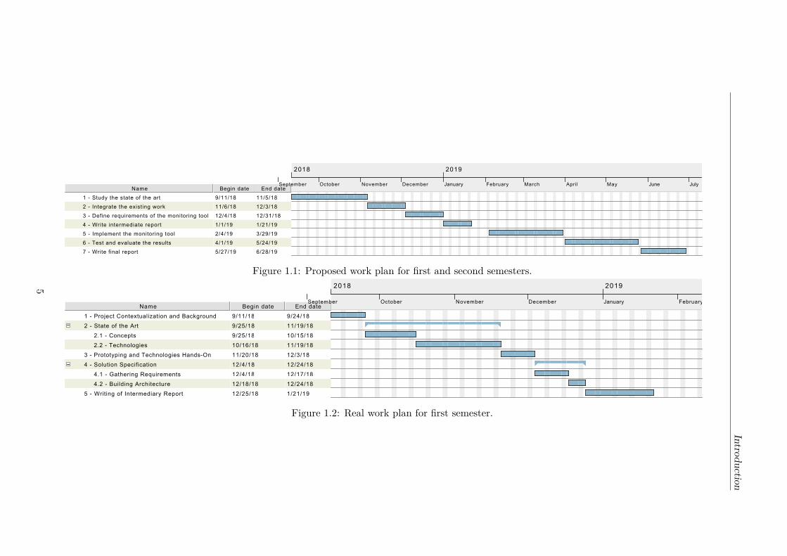
As we can see in Figures 1.1 and 1.2, the proposed work for the first semester hassuffered changes, when comparing it to the real work plan. Task 1 - Study the state ofthe art (Fig. 1.1), was branched in two, 1 - Project Contextualisation and Backgroundand 2 - State of the Art, however, these last ones tocked more time to accomplish due tolack of work in the field of trace processing and trace analysis, core topics for this thesis.Task 2 - Integrate the existing work (Fig. 1.1) was replaced by task 3 - Prototyping andTechnologies Hand-On (Fig. 1.2) due to redirections in the work course. This redirectionwas done due to interest increase in testing state of the art technologies, allowing us toget a better visualisation of the data provided by Huawei and enhancing our investigationwork. The remaining tasks took almost the predicted time to accomplish.
For the second semester, an “expected” work plan was defined with respect to theproposed work, presented in Figure 1.1, and the state of the research at the time. Theexpected work plan can be visualized in Figure 1.3. This Figure contains the expected(Grey) and real (Blue) work for the second semester.
Three main changes were made over time in the work plan. The first one involved areduction in task 1 - Metrics collector tool. When the solution was being implemented andthe prototype was capable to extract a set of metrics, we decided to stop the implementa-
3

Chapter 1
tion process to analyse the research questions. Second, this analysis lead to an emergenceof ideas, “2 - Restructuring research questions’,’ and thus a project redirection. Testswere removed from planning and the project followed with the objective of producing thedata analyser, “3 - Data Analyser tool”, and with it, answer two main questions regardinganomalous services and quality of tracing. Third, the introduction of a new task, “4 -Write paper to NCA 2019”, covering the work presented in this thesis.
4
Introduction
Name Begin date End date
1 - Study the state of the art 9/11/18 11/5/18
2 - Integrate the existing work 11/6/18 12/3/18
3 - Define requirements of the monitoring tool 12/4/18 12/31/18
4 - Write intermediate report 1/1/19 1/21/19
5 - Implement the monitoring tool 2/4/19 3/29/19
6 - Test and evaluate the results 4/1/19 5/24/19
7 - Write final report 5/27/19 6/28/19
2018 2019
September October November December January February March April May June July
Figure 1.1: Proposed work plan for first and second semesters.
Name Begin date End date
1 - Project Contextualization and Background 9/11/18 9/24/18
2 - State of the Art 9/25/18 11/19/18
2.1 - Concepts 9/25/18 10/15/18
2.2 - Technologies 10/16/18 11/19/18
3 - Prototyping and Technologies Hands-On 11/20/18 12/3/18
4 - Solution Specification 12/4/18 12/24/18
4.1 - Gathering Requirements 12/4/18 12/17/18
4.2 - Building Architecture 12/18/18 12/24/18
5 - Writing of Intermediary Report 12/25/18 1/21/19
2018 2019
September October November December January February
Figure 1.2: Real work plan for first semester.
5

Chapter
1
Name Begin date End date
1.a - Metrics collector tool (Expected) 2/4/19 5/3/19
1.1 - Setup project (Expected) 2/4/19 2/6/19
1.2 - Implement Controller (Expected) 2/7/19 2/18/19
1.3 - Implement Comunication (Expected) 2/19/19 2/22/19
1.4 - Implement File IO (Expected) 2/25/19 2/27/19
1.5 - Setup databases (Expected) 2/28/19 3/4/19
1.6 - Implement database repositories (Expected) 3/5/19 3/11/19
1.7 - Implement Graph Processor (Expected) 3/12/19 3/21/19
1.8 - Implement Logging Component (Expected) 3/22/19 3/26/19
1.9 - Research apropriate analysis algorithms (Expected) 3/27/19 4/11/19
1.10 - Implement Data Analyser (Expected) 4/12/19 4/23/19
1.11 - Define tests to be performed (Expected) 4/24/19 4/26/19
1.12 - Implement Testing Component (Expected) 4/29/19 5/3/19
1.b - Metrics collector tool 2/4/19 3/15/19
1.1 - Setup project (Real) 2/4/19 2/6/19
1.2 - Implement Logging Component (Real) 2/7/19 2/7/19
1.3 - Setup Docker Containers (Real) 2/8/19 2/8/19
1.4 - Implement Controller (Real) 2/11/19 2/20/19
1.5 - Implement File IO (Real) 2/21/19 2/25/19
1.6 - Implement Processors (Real) 2/26/19 3/4/19
1.7 - Setup databases (Real) 3/5/19 3/7/19
1.8 - Implement database repositories (Real) 3/8/19 3/12/19
1.9 - Implement metrics storage (Real) 3/13/19 3/15/19
2.a - Test and evaluate results (Expected) 5/6/19 5/27/19
2.1 - Run tests (Expected) 5/6/19 5/15/19
2.2 - Write analysis results (Expected) 5/16/19 5/27/19
2.b - Restructure research questions (Real) 3/18/19 3/27/19
2.1 - Write question analysis report (Real) 3/18/19 3/22/19
2.2 - Report review (Real) 3/25/19 3/27/19
3.a - Write final report (Expected) 5/28/19 6/28/19
3.b - Data analysis tool (Real) 3/28/19 5/17/19
3.1 - Quality of tracing analysis (Real) 3/28/19 4/3/19
3.1.1 - Time coverability testing (Real) 3/28/19 4/1/19
3.1.2 - Structure testing (Real) 4/2/19 4/3/19
3.2 - Research apropriate analysis algorithms (Real) 4/4/19 4/19/19
3.3 - Setup Jupyter notebooks (Real) 4/22/19 4/24/19
3.4 - Implement proposed solution and gather results (Real) 4/25/19 5/17/19
3.4.1 - Is there any anomalous service? (Real) 4/25/19 5/10/19
3.4.2 - Results gathering (Real) 5/13/19 5/17/19
4 - Write paper for NCA 2019 (Real) 5/20/19 5/29/19
5 - Write final report (Real) 5/30/19 6/28/19
2019
February March April May June Jul
Figure 1.3: Real and expected work plans for second semester.
6
Introduction
1.5 Research Contributions
From the work presented on this thesis, the following research contribution were made:
• Andre Bento, Jaime Correia, Ricardo Filipe, Filipe Araujo and Jorge Cardoso. Onthe Limits of Automated Analysis of OpenTracing. International Symposium onNetwork Computing and Applications (IEEE NCA 2019).
1.6 Document Structure
This section presents the document structure in this report, with a brief explanation ofthe contents in every section. This document contains a total of eight chapters, includingthis one, Chapter 1 - Introduction. The remaining six are presented as follows:
• In Chapter 2 - State of the Art the current state of the field for this kind of problem ispresented. This chapter is divided in three sections. The first one, Section 2.1 - Con-cepts introduces the reader to the core concepts to know as a requirement for a fullunderstanding of the topics discussed in this thesis. The second, Section 2.2 - Tech-nologies presents the result of a research for current technologies, that are able tohelp solving this problem and produce a proposed solution to be implemented. Fi-nally, Section 2.3 - Related Work presents the reader to related researches producedin the field of distributed tracing data handling.
• In Chapter 3 - Research Objectives and Approach the problem is approached indetail and the objectives of this research are presented. This chapter is divided intwo sections. First, Section 3.1 - Research Objectives, provides a concrete defini-tion of the problem, how we tackled it, the main difficulties that were found andthe objectives involved in order to propose a solution. Second, Section 3.2 - Re-search Questions, a compilation of questions are presented and evaluated with somereasoning about possible ways to answer them.
• In Chapter 4 - Proposed Solution a possible solution for the presented problem isexposed and explained in detail. This chapter is divided in four sections. Thefirst one, Section 4.1 - Functional Requirements, expose the functional requirementswith their corresponding priority levels and a brief explanation to every single oneof them. The second one, Section 4.2 - Quality Attributes, contains the gatherednon-functional requirements that were used to build the solution architecture. Thethird one, Section 4.3 - Technical Restrictions, presents the defined technical restric-tions for this project. The last one, Section 4.4 - Architecture, presents the possiblesolution architecture using some representational diagrams, and ends with an anal-ysis and validation to check if the presented architecture meets up the restrictionsinvolved in the architectural drivers.
• In Chapter 5 - Implementation Process, the implementation process of the possiblesolution is presented with detail. This chapter is divided in three main sections cov-ering the whole implementation process, from the input data set through the pair ofcomponents presented in the previous chapter. The first one, Section 5.1 - HuaweiTracing Data Set, the tracing data set provided by Huawei to be used as the core datafor research is exposed with some detail. Second, in Section 5.2 - OpenTracing Pro-cessor Component we present the possible solution for the first component, namely
7

Chapter 1
“Graphy OpenTracing processor (OTP)”, that processes and extracts metrics fromtracing data. The final Section 5.3 - Data Analysis Component presents the possi-ble solution for the second component, namely “Data Analyser”, that handles dataproduced by the first component and produces the analysis reports. Also, in the lasttwo sections presented, the used algorithms and methods in the implementations areproperly detailed and explained.
• In Chapter 6 - Research Objectives and Approach, the gathered results, correspond-ing analysis and limitations of tracing data are presented. This chapter is dividedin three main sections. The first one, Section 6.1 - Anomaly Detection, the resultsregarding the gathered observations on the extracted metrics of anomalous servicedetection are presented and explained. Second, in Section 6.2 - Trace Quality Analy-sis the results obtained from the quality analysis methods applied to the tracing dataset are presented and explained. The final Section 6.3 - Limitations of OpenTracingData we present the limitations felted when designing a solution to process tracingdata, more precisely OpenTracing data.
• Last, in Chapter 7 - Conclusion and Future Work, the main conclusions for thisresearch work are presented. To present this chapter, a reflection about the imple-mented tools, methods produced and the open paths from this research are exposed.Also a reflection of the main difficulties felted with this research regarding the han-dling of tracing data are presented. After this, the future work that can be addressed,considering this work, is properly explained.
Next, Chapter 2 - State of the Art, the state of the field is covered with core concepts,technologies and related work.
8

Chapter 2
State of the Art
In this Chapter, we discuss the core concepts regarding the project, the most moderntechnology for the purpose today and related work in the area. All the information pre-sented results from work of research through published articles, knowledge exchange andweb searching.
First, the main purpose of Section 2.1 - Concepts is to introduce and provide a briefexplanation about the core concepts to the reader. Second, Section 2.2 - Technologies, allthe relevant technologies are analysed and discussed. In the final Section 2.3 - RelatedWork, published articles and posts of related work are presented and possible researchdirections are discussed.
2.1 Concepts
The following concepts represents the baseline to understand the work related to thisresearch project. First an explanation of higher level of concepts that composes the titleof this thesis are presented in Subsections 2.1.1 and 2.1.2. The following Subsections 2.1.3to 2.1.5, aim to cover topics related to previous concepts: Distributed Tracing, Graphsand Time-Series.
2.1.1 Microservices
The term “micro web services” was first used by Dr. Peter Rogers during a conferenceon cloud computing in 2005, and evolved later on to “Microservices” at an event forsoftware architects in 2011, where the term was used to describe a style of architecturethat many attendees were experimenting with at the time. Netflix and Amazon wereamong the early pioneers of microservices [7].
Microservices is “an architectural style that structures an application as a collectionof loosely coupled services, which implement business capabilities” [1], [2].
This style of software development has a very long history and has being introducedand evolving due to software engineering achievements in the later years regarding clouddistributed computing infrastructures, Application Programming Interface (API) improve-ments, agile development methodologies and the emergence of the recent phenomenon ofcontainerized applications. “A container is a standard unit of software that packagesup code and all its dependencies so the application runs quickly and reliably from one
9

Chapter 2
computing environment to another, communicating with others through an API” [8].
In Microservices, services are small, specifically calibrated to perform a single func-tion, also each service is designed to be autonomous, resilient, minimal and composable.This framework brings a culture of rapid iteration, automation, testing, and continuousdeployment, enabling teams to create products and deploy code exponentially faster thanever before [9].
Until the rising of Microservices based architecture, the Monolithic architectural stylewas the most used. This style has a the particularity of produce software composed allin one piece. All features are bundled, packaged and deployed in a single tier applicationusing a single code base.
Figure 2.1 aims to give a comparison between both architectural styles, Monolithicand Microservices, and provide an insight about the differences between them.
Figure 2.1: Monolithic and Microservices architectural styles [10].
Both styles presented have their own advantages and disadvantages. To briefly presentsome of them, two examples are provided, one for each architectural style. First example:if one team needs to develop a single process system, e.g., e-Commerce application, thatauthorizes customer, takes an order, check products inventory, authorize payment andships ordered products. The best alternative is to use Monolithic architecture, becausethey can develop every feature in a single software package due to the application sim-plicity, however, if the client starts to demand hard changes and additional features inthe solution, the code base may tend to increase into “out of control”, leading to morechallenging and time consuming changes. Second example, if one team needs to developa complex and huge service that needs to scale, e.g., Video streaming service, the bestalternative is to use Microservices architecture, because they can tackle the problem ofcomplexity by decomposing the application into a set of manageable small services whichare much faster to develop and test by individual organized teams, and thus, it will beeasier to maintain the code base due to decoupling, however, it will be harder to monitor
10

State of the Art
and manage the entire platform due to additional complexity associated with distributedsystems.
Taking into consideration this increasing difficulty in monitoring and managing largeMicroservice based platforms, one must be aware and observe system behaviour to be ableto control it. Therefore, in the next Subsection 2.1.2, the core concept of Observabilityand Controlling Performance is explained.
2.1.2 Observability and Controlling Performance
This Subsection aims to provide an introduction to some theory concepts about Ob-servability and Performance Controlling, regarding distributed software systems.
Observability is a meaningfully extension of the word observing. Observing is “to beor become aware of, especially through careful and directed attention; to notice’ ’[11]. Theterm Observability comes from the world of engineering and control theory. Observabilityis not a new term in the industry, however it has gain more focus in the last years due toDevelopment and Operations (DevOps) raising. It means by definition “to measure of howwell internal states of a system can be inferred from knowledge of its external outputs” [12].Therefore, if our good old software systems and applications do not adequately externalizetheir state, then even the best monitoring can fall short.
Controlling in control systems is “to manage the behaviour of a certain system” [13].Controlling and Observability are dual aspects of the same problem [12], as we need tohave information to infer state and be able take action. E.g., When observing an expo-nential increase in the Central Processing Unit (CPU) load, the system scales horizontallyinvoking more machines and spreading the work between them to easy handle the work.This is a clear and simple example that conjugates the terms presented, we have: valuesthat are observed “Observability” and action that leads to system control “ControllingPerformance”.
When we want to understand the working and behaviour of a system, we need towatch it very closely and pay special attention to all details and information it provides.Microservice based systems produce multiple types of information if instrumented. Thesetype of information are the ones mentioned in Chapter 1: Monitoring, Tracing and Log-ging. In this thesis, the goal is to use tracing data thus, this type of produced informationis the one to focus.
In the next Subsection 2.1.3 - Distributed Tracing, the type of data mentioned beforeis presented and explained in detail.
2.1.3 Distributed Tracing
Distributed tracing [14] is a method that comes from traditional tracing, but applied toa distributed system at the work-flow level. It profiles and monitor applications, especiallythose built using microservice architectures and, in the end, it can be used to help DevOpsteams pinpoint where failures occur and why.
A number of tools and standards emerged from this concept. For example, the Open-Tracing standard [15] follows the model proposed by Fonseca et al. [16], which definestraces as a tree of spans representing scopes or units of work (i.e., thread, function, ser-vice). These traces enable following such units of work through the system.
11

Chapter 2
OpenTracing uses dynamic, fixed-width metadata to propagate causality between spans,meaning that each span has a trace identifier common to all spans of the same trace, aswell as a span identifier and parent identifier representing parent/child relationships be-tween spans [17]. The standard defines the format for spans and the semantic [18], [19]conventions for their content/annotations.
Figure 2.2 provides a clear insight about how spans are related to time and with eachother.
Span A
Span B
Span C
Span D
Span E
Time
Figure 2.2: Sample trace over time.
In Figure 2.2 there are a group of five spans spread through time that represents atrace. A trace is a group of spans that share the same TraceID. A trace is a representationof a data/execution path in the system. A span represents the logical unit of work in thesystem. A trace can also be a span, if there is only one span presented in the trace. Onespan can cause another.
Causality relationship between spans can be observed in Figure 2.2, where “Span A”causes “Span B” and “Span E”, moreover, “Span B” causes “Span C” and “Span D”. Fromthis we say that “Span A” is parent of “Span B” and “Span E”. Likewise, “Span B” and“Span E” are children of “Span A”. In this case, “Span A” does not have a parent, itis an “orphan span” and therefore, is the root span and the origin of this whole trace.Spans carry with them metadata like e.g., SpanID and ParentID, that allows to infer thisrelationships.
Disposition of spans over time is another clear fact that can be observed from therepresentation in Figure 2.2. Spans have a begin and an end in time. This causes them tohave a duration. Spans are spread through time, however they usually stay inside parentboundaries, this means that the duration of a parent span always covers durations of theirchildren. Considering a parent and a child spans, if they are related, the parent spanalways start before child span, also, the parent span always end after child span. Notethat nothing prevents multiple spans to start in the same exact moment. Span also carrywith them metadata like e.g., Timestamp and Duration, that allows to infer their positionin time and when they end.
An example of a span can be an Hypertext Transfer Protocol (HTTP) call or a RemoteProcedure Call (RPC) call. We may think of the following cases to define each operation
12

State of the Art
inherent to each box presented in Figure 2.2: A - “Get user info”, B - “Fetch user datafrom database”, C - “Connect to MySQL server”, D - “Can’t connect to MySQL server”and E - “Send error result to client”.
In the data model specification, the creators of OpenTracing say that: “with a coupleof spans, we might be able to generate a span tree and model a directed graph of a portionof the system” [15]. This is due to the causal relationships they represent. Apart from theroot span every other span must have a parent. Figure 2.3 provides an example of a spantree.
Span A Root Span
Span B Span E
Span C Span D
Figure 2.3: Span Tree example.
Figure 2.3 contains a span tree representation with a trace containing five spans. Apartfrom the root span every other span must have a parent. With this causal relationship,a path through the system can be retrieved. For example, if every span processes in adifferent endpoint represented by letters presented in the span tree, one may generate therequest path: A → B → D. This means that our hypothetical request passed throughmachine A, B and D, or if it were services, the request passed from service A, to B andfinally to D. From this, we can generate the dependency graph of the system (explainedin the Subsection 2.1.4 - Graphs).
This type of data is extracted as trace files or streamed over transfer protocols likee.g., HTTP, from technologies like Kubernetes [20], OpenStack [21], and other cloud ordistributed management system technologies that implements some kind of system orcode instrumentation using, for example, OpenTracing [22] or OpenCensus [23]. Tracingcontains some vital system details as they are the result of system instrumentation andtherefore, this data can be used as a resource to provide observability over the distributedsystem.
As said before, from the causality relationship between spans we can generate a de-pendency graph of the system. The next Subsection 2.1.4 - Graphs aims to provide a clearunderstand of this concept and how they relate with distributed tracing.
13
Chapter 2
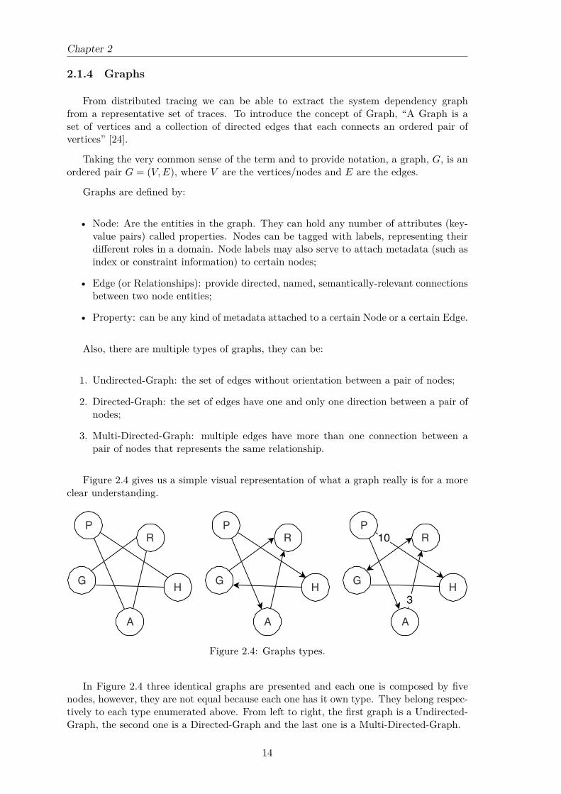
2.1.4 Graphs
From distributed tracing we can be able to extract the system dependency graphfrom a representative set of traces. To introduce the concept of Graph, “A Graph is aset of vertices and a collection of directed edges that each connects an ordered pair ofvertices” [24].
Taking the very common sense of the term and to provide notation, a graph, G, is anordered pair G = (V,E), where V are the vertices/nodes and E are the edges.
Graphs are defined by:
• Node: Are the entities in the graph. They can hold any number of attributes (key-value pairs) called properties. Nodes can be tagged with labels, representing theirdifferent roles in a domain. Node labels may also serve to attach metadata (such asindex or constraint information) to certain nodes;
• Edge (or Relationships): provide directed, named, semantically-relevant connectionsbetween two node entities;
• Property: can be any kind of metadata attached to a certain Node or a certain Edge.
Also, there are multiple types of graphs, they can be:
1. Undirected-Graph: the set of edges without orientation between a pair of nodes;
2. Directed-Graph: the set of edges have one and only one direction between a pair ofnodes;
3. Multi-Directed-Graph: multiple edges have more than one connection between apair of nodes that represents the same relationship.
Figure 2.4 gives us a simple visual representation of what a graph really is for a moreclear understanding.
G
R
A
P
H G
R
A
P
H G
R
3
A
10P
H
Figure 2.4: Graphs types.
In Figure 2.4 three identical graphs are presented and each one is composed by fivenodes, however, they are not equal because each one has it own type. They belong respec-tively to each type enumerated above. From left to right, the first graph is a Undirected-Graph, the second one is a Directed-Graph and the last one is a Multi-Directed-Graph.
14
State of the Art
The last graph has some numbers in some edges. Every graph can have this anno-tations. These can provide some information about the connection between the pair ofnodes. For example, in distributed systems context, if this graph represents our systemdependency graph, and nodes H and P hypothetical services, the edge between themcould represent calls between these two service and the notation number the number ofcalls with respect to the edge direction. Therefore, in this case, we would have 10 requestsfrom incoming from P to H.
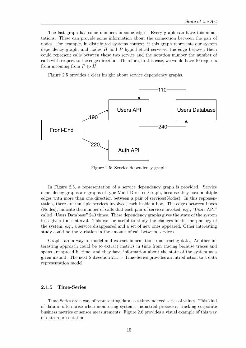
Figure 2.5 provides a clear insight about service dependency graphs.
190
220
Front-End 240
Users API
Auth API
110
Users Database
Figure 2.5: Service dependency graph.
In Figure 2.5, a representation of a service dependency graph is provided. Servicedependency graphs are graphs of type Multi-Directed-Graph, because they have multipleedges with more than one direction between a pair of services(Nodes). In this represen-tation, there are multiple services involved, each inside a box. The edges between boxes(Nodes), indicate the number of calls that each pair of services invoked, e.g., “Users API”called “Users Database” 240 times. These dependency graphs gives the state of the systemin a given time interval. This can be useful to study the changes in the morphology ofthe system, e.g., a service disappeared and a set of new ones appeared. Other interestingstudy could be the variation in the amount of call between services.
Graphs are a way to model and extract information from tracing data. Another in-teresting approach could be to extract metrics in time from tracing because traces andspans are spread in time, and they have information about the state of the system at agiven instant. The next Subsection 2.1.5 - Time-Series provides an introduction to a datarepresentation model.
2.1.5 Time-Series
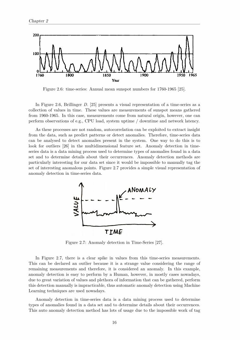
Time-Series are a way of representing data as a time-indexed series of values. This kindof data is often arise when monitoring systems, industrial processes, tracking corporatebusiness metrics or sensor measurements. Figure 2.6 provides a visual example of this wayof data representation.
15
Chapter 2
Figure 2.6: time-series: Annual mean sunspot numbers for 1760-1965 [25].
In Figure 2.6, Brillinger D. [25] presents a visual representation of a time-series as acollection of values in time. These values are measurements of sunspot means gatheredfrom 1960-1965. In this case, measurements come from natural origin, however, one canperform observations of e.g., CPU load, system uptime / downtime and network latency.
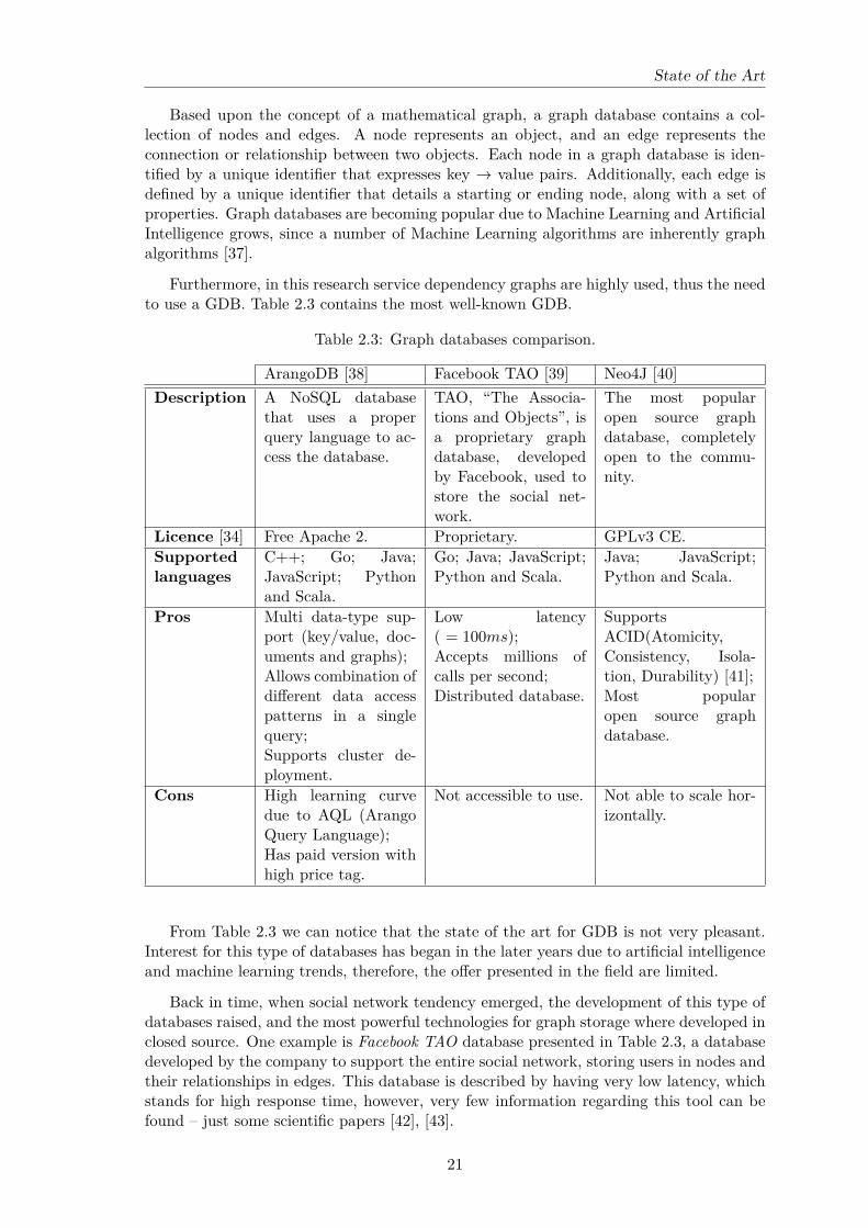
As these processes are not random, autocorrelation can be exploited to extract insightfrom the data, such as predict patterns or detect anomalies. Therefore, time-series datacan be analysed to detect anomalies present in the system. One way to do this is tolook for outliers [26] in the multidimensional feature set. Anomaly detection in time-series data is a data mining process used to determine types of anomalies found in a dataset and to determine details about their occurrences. Anomaly detection methods areparticularly interesting for our data set since it would be impossible to manually tag theset of interesting anomalous points. Figure 2.7 provides a simple visual representation ofanomaly detection in time-series data.
Figure 2.7: Anomaly detection in Time-Series [27].
In Figure 2.7, there is a clear spike in values from this time-series measurements.This can be declared an outlier because it is a strange value considering the range ofremaining measurements and therefore, it is considered an anomaly. In this example,anomaly detection is easy to perform by a Human, however, in mostly cases nowadays,due to great variation of values and plethora of information that can be gathered, performthis detection manually is impracticable, thus automatic anomaly detection using MachineLearning techniques are used nowadays.
Anomaly detection in time-series data is a data mining process used to determinetypes of anomalies found in a data set and to determine details about their occurrences.This auto anomaly detection method has lots of usage due to the impossible work of tag
16

State of the Art
manually the interesting set of anomalous points. Auto anomaly detection has a widerange of applications such as fraud detection, system health monitoring, fault detection,event detection systems in sensor networks, and so on.
After explaining the core concepts, foundations for the work presented in this thesis,to the reader, technologies capable of handling this types of information are presented anddiscussed in next Section 2.2 - Technologies.
2.2 Technologies
In this section are presented technologies and tools capable of handling the types ofinformation discussed in the previous Section 2.1 - Concepts.
The main tools covered are: 2.2.1 - Distributed Tracing Tools, for distributed trac-ing data handling, 2.2.2 - Graph Manipulation and Processing Tools and 2.2.3 - GraphDatabase Tools, for graph processing and storage, and 2.2.4 - Time-Series Database Tools,for time-series value storage.
2.2.1 Distributed Tracing Tools
This Subsection presents the most used and known distributed tracing tools. Thesetools are mainly oriented for tracing distributed systems like microservices-based applica-tions. What they do is to fetch or receive trace data from this kind of complex systems,treat the information, and then present it to the user using charts and diagrams in orderto explore the data in a more human-readable way. One of the best features presentedin this tools, is the possibility to perform queries on the tracing (e.g., by trace id and bytime-frame). Table 2.1 presents the most well-known open source tracing tools.
In Table 2.1, we can see that these two tools are very similar. Both are open sourceprojects, allow docker containerization and provide a browser ui to simplify user interac-tion. Jaeger was created by Uber and the design was based on Zipkin, however, it doesnot provide much more features. The best feature that was released for Jaeger in the pastyear was the capability of perform trace comparison, where the user can select a pair oftraces and compare them in terms of structure. This is a good effort in additional features,but it is short in versatility because we can only compare a pair of traces in a “sea” ofthousands, or even millions.
These tools aim to collect trace information and provide a user interface with somequery capabilities for DevOps to use. However they are always focused on span and tracelookup and presentation, and do not provide a more interesting analysis of the system,for example to determine if there is any problem related to some microservice presentedin the system. This kind of work falls into the user, DevOps, as they need to perform thetedious work of investigation and analyse the tracing with the objective of find anythingwrong with them.
This kind of tools can be a good starting point for the problem that we face, becausethey already do some work for us like grouping the data generated by the system andprovide a good representation for them.
In next Subsection 2.2.2, graph manipulation and processing tools are presented anddiscussed.
17

Chapter 2
Table 2.1: Distributed tracing tools comparison.
Jaeger [28] Zipkin [29]Brief description Released as open source by
Uber Technologies. Used formonitoring and troubleshoot-ing microservices-based dis-tributed systems. Was inspiredby Zipkin.
Helps gathering timing dataneeded to troubleshoot latencyproblems in microservice appli-cations. It manages both thecollection and lookup of thisdata. Zipkin’s design is basedon the Google Dapper paper.
Pros Open source;Docker-ready;Collector interface is compati-ble with Zipkin protocol;Dynamic sampling rate;Browser user interface.
Open source;Docker-ready;Allows multiple span transporttechnologies (HTTP, Kafka,Scribe, AMQP);Browser user interface.
Cons Only supports two span trans-port ways (Thrift and HTTP).
Fixed sampling rate.
Analysis Dependency graph view;Trace comparison (End 2018).
Dependency graph view.
Used by Red Hat;Symantec;Uber.
AirBnb;IBM;Lightstep.
2.2.2 Graph Manipulation and Processing Tools
Distributed tracing is a type of data produced by Microservice based architectures.This type of data is composed by traces and spans. With a set of related spans, a servicedependency graph can be produced. This dependency graph is a Multi-Directed-Graph,as presented in Subsection 2.1.4. Therefore, with this data at our disposal, there is theneed of a graph manipulation and processing tool.
In this Subsection, the state of the art about graph manipulation and processing toolsis presented. Graphs are non-linear data structure representations consisting of nodesand edges. Nodes are sometimes also referred to as vertices and edges are lines or arcsthat connect any pair of nodes in the graph. This data structure takes some particularapproaches when handling their contents, because there are some special attributes related.For example, perform the calculation of the degree of some node – degree of a node is thenumber of edges that connect to the node itself; Calculate how many nodes entered andexited the graph by comparing it to another one; Know the difference in edges betweentwo distinct graphs [30].
Taking into consideration this data structure, the particularities involved and the needto use graphs to manipulate service dependencies, frameworks with features capable ofhandling and retrieving graphs are a need. Therefore, Table 2.2 presents a comparison ofthe main tools available at the time for graph manipulation and processing.
18

State of the Art
Table 2.2: Graph manipulation and processing tools comparison.
Apache Giraph [31] Ligra [32] NetworkX [33]Description An iterative graph
processing systembuilt for high scala-bility. Currently usedat Facebook to anal-yse the social graphformed by users andtheir relationships.
A library collectionfor graph creation,analysis and manipu-lation of networks.
A Python package forthe creation, manipu-lation, and study ofstructure, dynamics,and functions of com-plex networks.
Licence [34] Free Apache 2. MIT. BSD - New License.Supportedlanguages
Java and Scala. C and C++. Python.
Pros Distributed and veryscalable;Excellent perfor-mance – Process onetrillion edges using200 modest machinesin 4 minutes.
Handles very largegraphs;Exploit large memoryand multi-core CPU –Vertically scalable.
Good support andvery easy to installwith Python;Lots of graph al-gorithms alreadyimplemented andtested.
Cons Uses “Think-Like-a-Vertex” programmingmodel that oftenforces into using sub-optimal algorithms,thus is quite limitedand sacrifices perfor-mance for scaling out;Unable to performmany complex graphanalysis tasks becauseit primarily supportsBulk synchronousparallel.
Lack of documenta-tion and therefore,very hard to use;Does not have manyusage in the commu-nity.
Not scalable (single-machine);High learning curvedue to the maturity ofthe project;Begins to slow downwhen processing highamount of data –400.000+ nodes.
Table 2.2 presents some key points to consider when choosing a graph manipulationand processing tool.
First, one aspect to be considered when comparing them is the scalability and perfor-mance that each provide. Apache Giraph is the best tool in this field, since it is imple-mented with distributed and parallel computation, which allows it to scale to multiple-machines, sharing the load between them, and processing data large quantities of datain less time than the remaining presented tools. On the opposite side, NetworkX, onlyworks in a single-machine environment which does not allow it scale to multiple-machines.Ligra, like the previous tool, works in a single-machine environment, however it benefitsfrom vertical scale on a single-machine, which allows to exploit multi-core CPU and largememory. NetworkX and Ligra are tools that can present a bottleneck in a system wherethe main focus is to handle large amounts of data in short times.
19

Chapter 2
Secondly, another aspect to be considered is the support and quantity of implementedgraph algorithms available on the frameworks. NetworkX have advantages in this aspect,because it contains implementation of the majority graph algorithms defined and studied ingraph and networking theory. Also, due to project maturity, it has a good documentationsupport from the community who keeps all the information updated. Ligra framework haslack of documentation, which causes tremendous difficulty for developers to use and knowwhat are the implemented features. Apache Giraph, does not support a large set of graphprocessing algorithms due to implementation constraints.
Figure 2.8 gives a clear insight when comparing these tools from two features – scala-bility / performance against implementation of graph algorithms.
Figure 2.8: Graph tools: Scalability vs. Algorithm implementation [35].
In Figure 2.8 we can observe tools disposition regarding the two aspect key pointsexplained before. This figure contains all tools presented over two featured axis: onefor scalability and the other for implementation of graph algorithms. Tools placementin this chart proves and reinforces the comparison presented before. Apache Giraph andNetworkX are placed in the edges of these features, which means that Apache Giraphcan be found in the upper left region of the chart – highly distributed but minimally ingraph algorithms implementation –, and NetworkX is in the lower right region – minimallydistributed but highly in graph algorithms implementation.
After discussing tools capable of manipulate and process graphs, their storage is aneed for later usage. Graph Database (GDB) storage technologies are presented in nextSubsection 2.2.3 - Graph Database Tools.
2.2.3 Graph Database Tools
Graph databases represent a way of persisting graph information. After having instan-tiated a Graph, processed it in volatile memory, they can be stored in persistent memoryfor later use. To do this one can use a GDB. A GDB is “a database that allows graph datastoring and uses graph structures for semantic queries with nodes, edges and propertiesto represent them” [36].
20
State of the Art
Based upon the concept of a mathematical graph, a graph database contains a col-lection of nodes and edges. A node represents an object, and an edge represents theconnection or relationship between two objects. Each node in a graph database is iden-tified by a unique identifier that expresses key → value pairs. Additionally, each edge isdefined by a unique identifier that details a starting or ending node, along with a set ofproperties. Graph databases are becoming popular due to Machine Learning and ArtificialIntelligence grows, since a number of Machine Learning algorithms are inherently graphalgorithms [37].
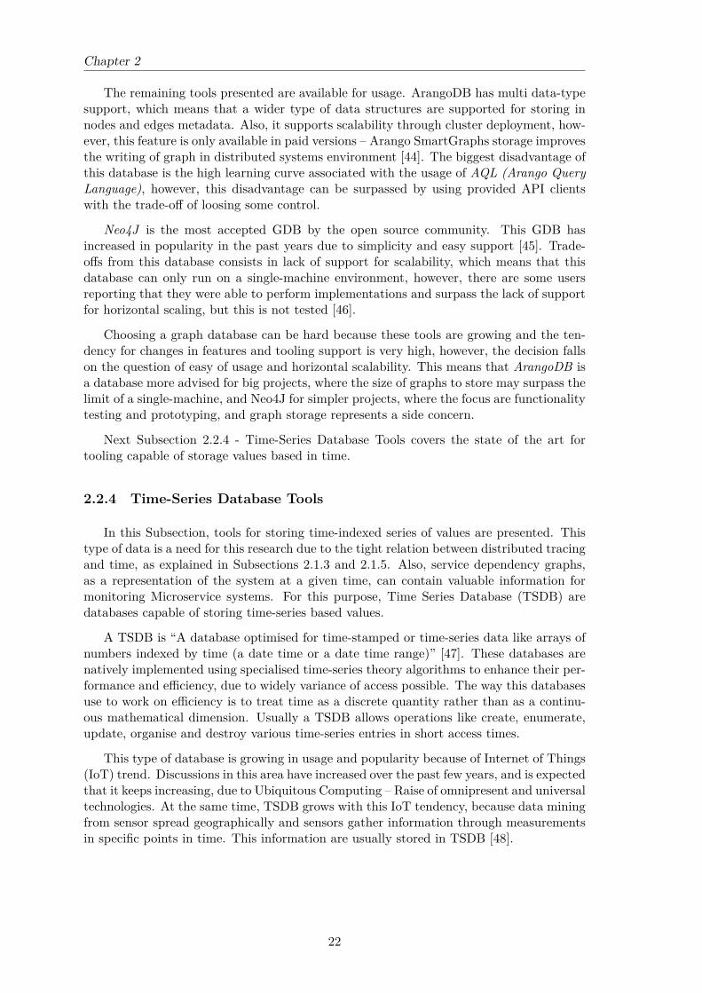
Furthermore, in this research service dependency graphs are highly used, thus the needto use a GDB. Table 2.3 contains the most well-known GDB.
Table 2.3: Graph databases comparison.
ArangoDB [38] Facebook TAO [39] Neo4J [40]Description A NoSQL database
that uses a properquery language to ac-cess the database.
TAO, “The Associa-tions and Objects”, isa proprietary graphdatabase, developedby Facebook, used tostore the social net-work.
The most popularopen source graphdatabase, completelyopen to the commu-nity.
Licence [34] Free Apache 2. Proprietary. GPLv3 CE.Supportedlanguages
C++; Go; Java;JavaScript; Pythonand Scala.
Go; Java; JavaScript;Python and Scala.
Java; JavaScript;Python and Scala.
Pros Multi data-type sup-port (key/value, doc-uments and graphs);Allows combination ofdifferent data accesspatterns in a singlequery;Supports cluster de-ployment.
Low latency( = 100ms);Accepts millions ofcalls per second;Distributed database.
SupportsACID(Atomicity,Consistency, Isola-tion, Durability) [41];Most popularopen source graphdatabase.
Cons High learning curvedue to AQL (ArangoQuery Language);Has paid version withhigh price tag.
Not accessible to use. Not able to scale hor-izontally.
From Table 2.3 we can notice that the state of the art for GDB is not very pleasant.Interest for this type of databases has began in the later years due to artificial intelligenceand machine learning trends, therefore, the offer presented in the field are limited.
Back in time, when social network tendency emerged, the development of this type ofdatabases raised, and the most powerful technologies for graph storage where developed inclosed source. One example is Facebook TAO database presented in Table 2.3, a databasedeveloped by the company to support the entire social network, storing users in nodes andtheir relationships in edges. This database is described by having very low latency, whichstands for high response time, however, very few information regarding this tool can befound – just some scientific papers [42], [43].
21
Chapter 2
The remaining tools presented are available for usage. ArangoDB has multi data-typesupport, which means that a wider type of data structures are supported for storing innodes and edges metadata. Also, it supports scalability through cluster deployment, how-ever, this feature is only available in paid versions – Arango SmartGraphs storage improvesthe writing of graph in distributed systems environment [44]. The biggest disadvantage ofthis database is the high learning curve associated with the usage of AQL (Arango QueryLanguage), however, this disadvantage can be surpassed by using provided API clientswith the trade-off of loosing some control.
Neo4J is the most accepted GDB by the open source community. This GDB hasincreased in popularity in the past years due to simplicity and easy support [45]. Trade-offs from this database consists in lack of support for scalability, which means that thisdatabase can only run on a single-machine environment, however, there are some usersreporting that they were able to perform implementations and surpass the lack of supportfor horizontal scaling, but this is not tested [46].
Choosing a graph database can be hard because these tools are growing and the ten-dency for changes in features and tooling support is very high, however, the decision fallson the question of easy of usage and horizontal scalability. This means that ArangoDB isa database more advised for big projects, where the size of graphs to store may surpass thelimit of a single-machine, and Neo4J for simpler projects, where the focus are functionalitytesting and prototyping, and graph storage represents a side concern.
Next Subsection 2.2.4 - Time-Series Database Tools covers the state of the art fortooling capable of storage values based in time.
2.2.4 Time-Series Database Tools
In this Subsection, tools for storing time-indexed series of values are presented. Thistype of data is a need for this research due to the tight relation between distributed tracingand time, as explained in Subsections 2.1.3 and 2.1.5. Also, service dependency graphs,as a representation of the system at a given time, can contain valuable information formonitoring Microservice systems. For this purpose, Time Series Database (TSDB) aredatabases capable of storing time-series based values.
A TSDB is “A database optimised for time-stamped or time-series data like arrays ofnumbers indexed by time (a date time or a date time range)” [47]. These databases arenatively implemented using specialised time-series theory algorithms to enhance their per-formance and efficiency, due to widely variance of access possible. The way this databasesuse to work on efficiency is to treat time as a discrete quantity rather than as a continu-ous mathematical dimension. Usually a TSDB allows operations like create, enumerate,update, organise and destroy various time-series entries in short access times.
This type of database is growing in usage and popularity because of Internet of Things(IoT) trend. Discussions in this area have increased over the past few years, and is expectedthat it keeps increasing, due to Ubiquitous Computing – Raise of omnipresent and universaltechnologies. At the same time, TSDB grows with this IoT tendency, because data miningfrom sensor spread geographically and sensors gather information through measurementsin specific points in time. This information are usually stored in TSDB [48].
22

State of the Art
Table 2.4 presents a comparison between two TSDB: InfluxDb and OpenTSDB.
Table 2.4: Time-series databases comparison.
InfluxDB [49] OpenTSDB [50]Description An open-source time-series
database written in Go and op-timised for fast, high-availabilitystorage and retrieval of time-series data in fields such asoperations monitoring, applica-tion metrics, Internet of Thingssensor data, and real-timeanalytics’s.
A distributed and scalable TSDBwritten on top of HBase;OpenTSDB was written to ad-dress a common need: store, in-dex and serve metrics collectedfrom computer systems (networkgear, operating systems and ap-plications) at a large scale, there-fore, making this data easily ac-cessible and displayed.
Licence [34] MIT. GPL.Supportedlanguages
Erlang, Go, Java, JavaScript,Lisp, Python, R and Scala.
Erlang, Go, Java, Python, R andRuby.
Pros Scalable in the enterprise ver-sion;Outstanding high performance;Accepts data from HTTP, TCP,and UDP protocols;SQL like query language;Allows real-time analytics’s.
Massively scalable;Great for large amounts of time-based events or logs;Accepts data from HTTP andTCP protocols;Good platform for future analyt-ical research into particular ag-gregations on event / log data;Does not have paid version.
Cons Enterprise high price tag;Clustering support only availablein the enterprise version.
Hard to set up;Not a good choice for general-purpose application data.
From Table 2.4, we can notice some similarities between these two TSDB databases.Both TSDB are capable scalable and accept HTTP and TCP transfer protocols for com-munication. InfluxDB and OpenTSDB are two open source time-series databases, how-ever, the first one, InfluxDB, is not completely free, as it has an enterprise paid version,which is not very visible in the offer. This enterprise version offers, clustering support,high availability and scalability [51], features that OpenTSDB offer for free. In termsof performance, InfluxDB surpasses and outperforms OpenTSDB in almost every bench-marks [52]. OpenTSDB has the benefits of being completely free and support the mostrelevant features, however it is very hard to set up and to develop for this database.
In the end, both TSDB are bundled with good features, and the decision falls into howmuch performance is needed when choosing one. If the need is performance and access tothe database in short amounts of time, with low latency responses, InfluxDB is the wayto go, by other way, if there no restriction about the performance needed to query thedatabase and money is a concern, the choice should be OpenTSDB.
Tooling for this project is presented. We have covered the most used technologies andcore concepts in related to the field of tracing Microservices. Next Section 2.3 - RelatedWork, will cover the related work performed in this area. Some ideas, approaches anddeveloped solutions will be discussed.
23
Chapter 2
2.3 Related Work
This section aims to present the related work in the field of distributed tracing datahandling and analysis. It is divided in three Subsections: first, 2.3.1 - Mastering AIOps,which covers a work carried out by Huawei, that uses machine learning – deep learning– methods to analyse data from distributed traces. Secondly, 2.3.2 - Anomaly Detectionusing Zipkin Tracing Data, a work of performed by Salesforce with the objective of analysetracing from a distributed tracing tool. Finally, 2.3.3 - Analysing distributed trace data,a work by Pinterest, where the objective is to study latency in tracing data.
2.3.1 Mastering AIOps
Distributed tracing has only started to gain widespread acceptance in the industryrecently, as a result of new architectural and software engineering practices, such as cloud-native, fine-grained systems and agile methodologies. Additionally, the increase in com-plexity resulting from the rise of web-scale distributed applications is a recent phenomenon.As a consequence of its novelty, there has been little research in the field so far.
A recent example, AIOps, an application of Artificial Intelligence to operations [53] wasintroduced in 2016 [54]. This trend aims to use Artificial Intelligence for IT Operationsin order to develop new methods to automate the enhance IT Operations. Driving this“revolution” are the following points:
• First there is the additional difficulty of manually managing distributed infrastruc-tures and system state;
• Secondly, the amount of data that has to be retained is increasing, creating a plethoraof problems to the operators handling it;
• Third, the infrastructure itself is becoming more distributed across geography andorganizations, as evidenced by trends like cloud-first development and fog computing;
• Finally, due to the overwhelming amount of new technologies and frameworks, it isan herculean task for operators to keep in pace with the new trends.
The work performed and presented by Huawei, entitled Mastering AIOps with DeepLearning, Time-Series Analysis and Distributed Tracing [55], aims to use distributed trac-ing data and aforementioned technologies to detect anomalous tracing. The proposedmethod encodes the traces and trains a deep learning neural network to detect significantdifferences in tracing. This is a very perceptive approach, taking into account the amountsof data that is needed to analyse, however is limited to classifying a trace as normal orabnormal, losing detail and interpretability i.e., no justification for the classification.
2.3.2 Anomaly Detection using Zipkin Tracing Data
Tooling in this field are not taking the expected relevance. Their usage is starting inindustry and production environments involving distributed systems, however, the con-cerns in are not well aligned with the needs of operators, and this leads to increasing effortwhen monitoring large scale and complex architectures, such as Microservices.
24
State of the Art
In a post from Salesforce, a work of research about using tracing data gathered byZipkin, to detect some anomalies in a Microservice based system [56]. At Salesforce,Zipkin is used to perform distributed tracing for Microservices, collecting traces fromtheir systems and providing performance insights in both production monitoring and pre-production testing. However, the current Zipkin open source instrumentation and UI offersonly primitive data tracing functionality and does not have in-depth performance analysisof the span data. The focus on their work was to detect and identify potential networkbottlenecks and microservices performance issues.
The approach carried out was to implement scripts using that used Python AI pack-ages, with the objective of extracting values from their network of services, namely servicedependency graph, in order to identify high traffic areas in the network. The values thatwere extracted were the number of connections from each service, which means, the degreeof the service at specific times. This allows to notice which services are establishing moreconnections with other services.
From this approach, it was possible to visualize the high traffic areas within the produc-tion network topology. Therefore, they have identified services with the most connections.This finding was an helpful feedback for service networking architects that designed thosemicroservices. Those services, identified with too many connections, may potentially be-come choking points in the system design. If one of the services fail, a huge impact on alarge number of depending services occur. Additionally, there could be also potential per-formance impacts in the system since a large number of services depending on them. Thoseare valuable information for system designers and architect to optimize their designs.
The conclusions from Salesforce research identified that, with Zipkin tracing data, it ispossible to identify network congestion, bottlenecks, efficiencies and the heat map in theproduction network. However, this tool does not provide analysis of tracing data at thislevel. This was the main conclusion and possible working direction from this research:“features like the ones presented, can be added to Zipkin or other distributed tracing toolproduct line, including UI and dashboards. Capabilities like daily metrics or correlationbetween microservices load and latency, able to generate alerts if bottleneck or heat mapis identified, should be added” [56].
2.3.3 Analysing distributed trace data
At Pinterest, the focus was to research for latency problems in their Microservicessolution. Pinterest claims to have tens of services and hundreds of network calls per-trace.One big problem identified at start is the huge difficulty of looking to trace data due tothe overwhelming quantity of information – “thousands of traces logged each minute (letalone the millions of requests per minute these traces are sampled from)”.
Pinterest felt the problem of monitoring Microservices early due to their service popu-larity in the past years. With this popularity, systems usage increased significantly. Thislead them to take action and create their closed source distributed tracing analysis toolcalled “Pintrace Trace Analyser” [57].
This tool gathers tracing data from Distributed Tracing Tools, more precisely fromZipkin, and processes a sample of these tracing to detect mainly latency problems in theservice dependency network. Looking at stats from thousands of traces over a longerperiod of time not only weeds out the outliers/buggy traces, but provides a holistic viewof performance.
25

Chapter 2
The conclusions from Pinterest, where that there is a great need to develop toolingfor distributed tracing analysis, with the main objective of ease the life of operators. Thefollowing points were considered:
1. Automatically generate reports so engineers can easily check the status of each de-ployment;
2. Setting up alerts for when latency or number of calls hits a certain threshold.
2.3.4 Research possible directions
One thing to notice from the related work presented is that there is few researchaccomplished in the area and trace tooling development, however, these works are fromthe past year and the tendency is to increase in the following years. Enlargement andusage of distributed systems are fuel to feed the need of research in this field and developnew methodologies and tools to monitor and control operations.
From the first work presented, “Mastering AIOps”, some final results and conclusionswere provided. They point out that the benefits of this approach were: first, very highaccuracy in detection 99, 7%, and secondly, extremely fast detection in O(n) time. How-ever, some limitations involving requiring very long training times for long traces (withdecent machines) were noted. Also, improvements were pointed: truncate traces, to lowerthe quantity of tracing and therefore, summarizing traces.
The second work presented, “Anomaly Detection using Zipkin Tracing Data”, pointdown the lack of features in the existing tools. These features include automatic anomalydetection using distributed tracing data. The main idea consists in extending functionalitypresented in this tools, to provide autonomous anomaly detection and alerting based oninformation presented in tracing from services.
The third work presented, “Analysing distributed trace data”, crucial points consideredwere to represent autonomous generation of reports, allowing operators to check the statusof deployments, and therefore, providing more control over the system regarding detectionof anomalous values in service latency.
Finally, from the multiple related work presented the final assumptions for possibleresearch directions in this field are:
• Focus on the most important traces, reducing the quantity of tracing;
• Develop new methods that leverage features of existing distributed tracing tools;
• Automate the detection of anomalies presented in distributed systems;
After providing the state of the art for this research to the reader, next Chapter 3 - Re-search Objectives and Approach will cover the objectives of this research, the approachused to tackle the problem and the compiled research questions.
26
Chapter 3
Research Objectives and Approach
In this Chapter, the problem is approached in detail and the objectives for this researchare presented. The problem definition, how we tackled it and our main difficulties andthe objectives involved to provide a possible solution are presented in Section 3.1 - Re-search Objectives. Also, a compilation of research questions are presented and evaluatedwith some reasoning about possible ways to answer them, later in Section 3.2 - ResearchQuestions.
3.1 Research Objectives
Modern distributed services are large, complex, and increasingly built upon other sim-ilarly complex distributed services. Debugging systems is not an easy task to perform.It involves the collection, interpretation, and display of information concerning the inter-actions among concurrently executing processes operating in distributed machines. Dis-tributed Tracing data helps keeping an history of work performed by these systems.
End-to-end tracing captures the causally-related activity (e.g., work done to process arequest) within and among the components of a distributed system. As distributed systemsgrow in scale and complexity, such tracing is becoming a critical tool for management taskslike diagnosis and resource accounting. However, as systems grow, resulting tracing datafrom system execution is growing as well [17].
Tracing data growth raises some problems. This data is used by system operators togain insight and observability of the distributed system, however, with this tendency toincrease in quantity and complexity, it is becoming an overwhelming task for operators.
There are some tools that help handling tracing data, such as the ones presented inSubsection 2.2.1 - Distributed Tracing Tools, however, they only perform the job of col-lecting tracing data, present this information to the user in more human-readable formatsand provide forms of querying this type of data. For this reason, manually managingthese growing microservice architectures is becoming an outdated approach due to theirincomportability.
To address this issue, there is a great need of improving tracing data processing andautomate the task of tracing analysis. However, at this point, we did not have any tracingdata at our disposal to start working, thus acquire tracing data from a distributed systemwas an urgency. Obtain tracing data for study is hard because it represents workingfrom these systems and contain confidential information about them. However, through a
27
Chapter 3
NDA (Non-Disclosure Agreement) and the help of professor Jorge Cardoso, representingHuawei, we were able to gain access to confidential tracing data generated by the company.To ensure confidentiality, in this thesis, direct data fields are presented using fictitiousinformation.
This tracing data set was the starting point for this research. It is in OpenTracingformat and was provided by Huawei. This data had been gathered from an experimentalOpenStack cluster used by the company for testing purposes, and covered two days ofoperation. This data is addressed in detail in Section 5.1 - Huawei Tracing Data Set.
After having access to tracing data, we have developed some prototype tools for dataingestion and setted up a distributed tracing tool. Zipkin was used as a distributedtracing tool to ingest tracing data provided by Huawei. The decision to use Zipkin insteadof Jaeger, fell in the fact that it were much simpler due to lesser feature configuration.This was done with the purpose of gain a clear visualization about the data that weregiven. From this we decided to perform several meetings with the objective of defining aresearch direction and be able to propose a solution.
In these meetings, the elements of this research project gathered to debate ideas anddefine a set of questions to answer, taking into consideration the defined problem. ProfessorJorge Cardoso, representing Huawei, was the client of the designed solution. The approachtaken was to create a shared Kanban Board [58], containing multiple lanes, to performthe of generation and refinement of prototype questions. This process involved havingprototype question in the first lane, and move them through every lane reaching the lastone, transforming a prototype question into a final research question. These researchquestions were built taking into consideration:
1. Main needs felt by operators in normal day-to-day tasks, troubleshooting distributedsystems;
2. Most common issues presented in these systems;
3. Variables involved when these issues appear;
4. Relationship between these variables and the most common issues.
In the next Section 3.2 - Research Questions, the process to generate the researchquestions is explained and the research questions, in their final state, are presented.
3.2 Research Questions
In this Section, we start by explaining the process to generate the research questions.In the end, these questions are defined and a possible approach for each one of them isdiscussed.
A Kanban Board was created with five lanes: “Initial Prototype”, “To Refine (1)”,“Interesting”, “To Refine (2)” and “Final Research Questions”. Throughout these lanes,questions were improved and filtered before reaching their final state.
Initial prototype questions were generated based on the four points enumerated at theend of the previous Section 3.1. Therefore, prototype questions where:
28
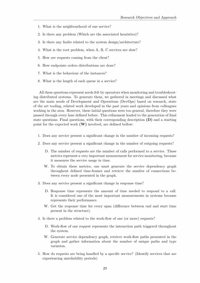
Research Objectives and Approach
1. What is the neighbourhood of one service?
2. Is there any problem (Which are the associated heuristics)?
3. Is there any faults related to the system design/architecture?
4. What is the root problem, when A, B, C services are slow?
5. How are requests coming from the client?
6. How endpoints orders distributions are done?
7. What is the behaviour of the instances?
8. What is the length of each queue in a service?
All these questions represent needs felt by operators when monitoring and troubleshoot-ing distributed systems. To generate them, we gathered in meetings and discussed whatare the main needs of Development and Operations (DevOps) based on research, stateof the art tooling, related work developed in the past years and opinions from colleaguesworking in the area. However, these initial questions were too general, therefore they werepassed through every lane defined before. This refinement leaded to the generation of finalstate questions. Final questions, with their corresponding description (D) and a startingpoint for the expected work (W) involved, are defined bellow:
1. Does any service present a significant change in the number of incoming requests?
2. Does any service present a significant change in the number of outgoing requests?
D. The number of requests are the number of calls performed to a service. Thesemetrics represent a very important measurement for service monitoring, becauseit measures the service usage in time.
W. To obtain these metrics, one must generate the service dependency graphthroughout defined time-frames and retrieve the number of connections be-tween every node presented in the graph.
3. Does any service present a significant change in response time?
D. Response time represents the amount of time needed to respond to a call.It is considered one of the most important measurements in systems becauserepresents their performance.
W. Get the response time for every span (difference between end and start timepresent in the structure).
4. Is there a problem related to the work-flow of one (or more) requests?
D. Work-flow of one request represents the interaction path triggered throughoutthe system.
W. Generate service dependency graph, retrieve work-flow paths presented in thegraph and gather information about the number of unique paths and typevariation.
5. How do requests are being handled by a specific service? (Identify services that areexperiencing unreliability periods)
29

Chapter 3
D. In the end, requests have success or not. This is represented by a status codein Hypertext Transfer Protocol (HTTP) or an exception in Remote ProcedureCall (RPC). Measure the ratio of these values can help identify unreliabilityperiods in services.
W. Gather status codes or exceptions from spans and generate a ratio of successand error.
6. Which services are the most popular in the system? (Number of established connec-tions)
D. Popularity of a service stands for the number of established connections. Thismeasurement is important because a failure in a very popular service can com-promise the entire system.
W. Generate service dependency graph, and calculate the degree of each node.Services with higher degree are the most popular in the system.
7. Does any service present a significant change in the services it uses to fulfil requests?
D. Services tend to communicate with a set of other services. These services donot change often, therefore, patterns in service communication can be observed.If these patterns are violated without service redeployment and networkingchanges, one might be facing a possible traffic redirection.
W. Generate service dependency graph, and retrieve the set of services that eachservice communicates. Gathering these values in time, lead to a history of com-munication between services and, therefore, pattern recognition can be appliedto detect strange variations.
8. Is there a problem related to the constitution of the system?
D. Constitution in microservices architecture represent which services are pre-sented in the system. The study of entries and exits of services in the overallsystem network can help identifying problems in system constitution.
W. Generate service dependency graph in consecutive time-frames and retrieve theentry / exit of services. Variation analysis of this data can lead to detectconstitution problems presented in distributed systems.
9. Do traces follow OpenTracing specification? (Structural quality testing)
D. Structure quality is always an important factor when using some dataset toanalyse a system. This question aims to perform a structural test of spanspresented in tracing against the defined specification.
W. Produce a structural schema based on the proposed open source tracing speci-fication – OpenTracing –, and check every span.
10. How is time coverage of tracing? (Coverability quality testing)
D. Time coverage is an important aspect in tracing, because this measurement canpinpoint possible failures in system instrumentation.
W. In tracing, child spans should cover almost the total duration of their parentspan. To perform this test, a span tree for each trace must be assembled andtimes ratios of the durations must be extracted.
30

Research Objectives and Approach
After having generated these final state questions, an analysis report was performedin order to group them in similar fields of end-to-end tracing use cases [17]. Table 3.1present the defined groups and the associated questions.
Table 3.1: Final state questions groups.
Group Question numbers1. Anomaly detection 1. Does any service present a significant change in
the number of incoming requests?2. Does any service present a significant change inthe number of outgoing requests?3. Does any service present a significant change inresponse time?
2. Steady state problems 4. Is there a problem related to the work-flow ofone (or more) requests?5. How do requests are being handled by a specificservice? (Identify services that are experiencingunreliability periods)
3. Distributed resource profiling 6. Which services are the most popular in the sys-tem? (Number of established connections)7. Does any service present a significant change inthe services it uses to fulfil requests?8. Is there a problem related to the constitution ofthe system?
4. Quality of tracing 9. Do traces follow OpenTracing specification?(Structural quality testing);10. How is time coverage of tracing? (Coverabilityquality testing).
Table 3.1 presents us with questions grouped in four classes: anomaly detection, steadystate problems, distributed resource profiling and quality of tracing. Questions were groupedin these four mentioned classes due to their affinity. The first one, Anomaly detection,is “diagnosis-related case that involves identifying and debugging problems related tocorrectness (e.g., component time-outs or connection failures)”, therefore grouped ques-tions are related with response time and number of calls performed to services. Secondly,Steady state problems, is “another diagnosis-related, which involves identifying and de-bugging problems that manifest in work-flows (and so are not anomalies)”, thus questionsare related with work-flow and status of requests. Thirdly, Distributed resource profiling,is “identify slow components or functions.”, so questions associated with service usageand system constitution. Finally, Quality of tracing, involve questions related to tracingquality testing.
The following general questions were composed for each group:
• Group 1 - Is there any anomalous service?
• Group 2 - What is the overall reliability of the service?
• Group 3 - Which service consumes more time when considering the entire set ofrequests?
• Group 4 - How can we measure the quality of tracing?
31

Chapter 3
From these general questions, we decided to tackle two groups: 1. Anomaly detectionand 4. Quality of tracing and therefore, the selected general questions were: 1. Is thereany anomalous service? and 4. How can we measure the quality of tracing?. Questionspresented in the remaining groups were not studied further in this research project.
The first question can be reduced to finding anomalies in observations of service orsystem behaviour, namely metrics and morphology. In particular, we considered threemetrics: number of incoming service calls, outgoing service calls and average response time.Our proposed solution in Chapter 4 - Proposed Solution must have this into consideration– extract and analyse these metrics from tracing data.
For the second question, there are multiple ways to analyse quality in tracing. Weexplore two directions, first performing a trace structure testing against the defined Open-Tracing specification –structural testing –, to determine if the tracing data complies withall the predefined requirements. Secondly, coverage testing for tracing data to determinehow much of the duration of Span is covered by its children – time coverability testing.The first kind would be more valuable if the specification was stricter, however, changingthe standard was not an option at the time as the data had external providence – discussedin Chapter 7 - Conclusion and Future Work.
Next Chapter 4 - Proposed Solution covers our proposed solution, taking into consid-erations the main problem, the data to process and the research questions to be answeredin this project.
32
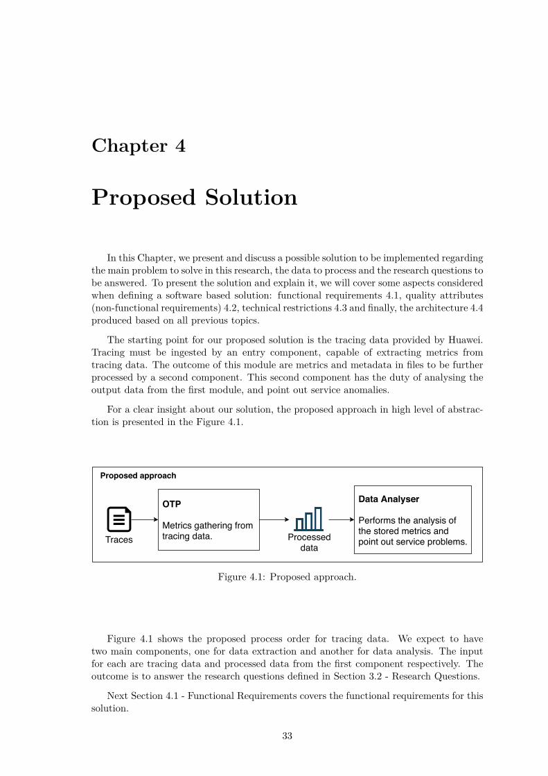
Chapter 4
Proposed Solution
In this Chapter, we present and discuss a possible solution to be implemented regardingthe main problem to solve in this research, the data to process and the research questions tobe answered. To present the solution and explain it, we will cover some aspects consideredwhen defining a software based solution: functional requirements 4.1, quality attributes(non-functional requirements) 4.2, technical restrictions 4.3 and finally, the architecture 4.4produced based on all previous topics.
The starting point for our proposed solution is the tracing data provided by Huawei.Tracing must be ingested by an entry component, capable of extracting metrics fromtracing data. The outcome of this module are metrics and metadata in files to be furtherprocessed by a second component. This second component has the duty of analysing theoutput data from the first module, and point out service anomalies.
For a clear insight about our solution, the proposed approach in high level of abstrac-tion is presented in the Figure 4.1.
Proposed approach
aaaMMM
OTP
Metrics gathering fromtracing data.Traces Processed
data
Data Analyser
Performs the analysis ofthe stored metrics andpoint out service problems.
Figure 4.1: Proposed approach.
Figure 4.1 shows the proposed process order for tracing data. We expect to havetwo main components, one for data extraction and another for data analysis. The inputfor each are tracing data and processed data from the first component respectively. Theoutcome is to answer the research questions defined in Section 3.2 - Research Questions.
Next Section 4.1 - Functional Requirements covers the functional requirements for thissolution.
33
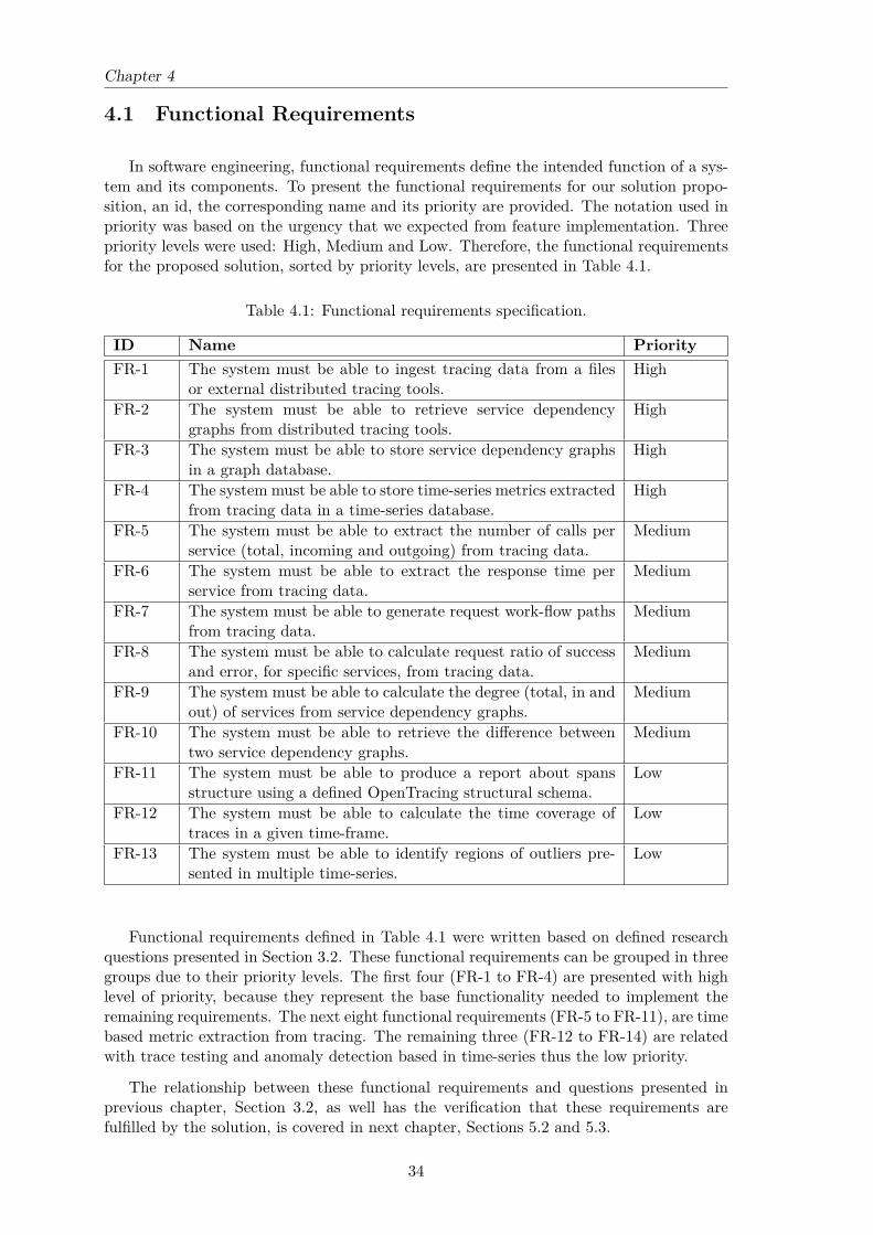
Chapter 4
4.1 Functional Requirements
In software engineering, functional requirements define the intended function of a sys-tem and its components. To present the functional requirements for our solution propo-sition, an id, the corresponding name and its priority are provided. The notation used inpriority was based on the urgency that we expected from feature implementation. Threepriority levels were used: High, Medium and Low. Therefore, the functional requirementsfor the proposed solution, sorted by priority levels, are presented in Table 4.1.
Table 4.1: Functional requirements specification.
ID Name PriorityFR-1 The system must be able to ingest tracing data from a files
or external distributed tracing tools.High
FR-2 The system must be able to retrieve service dependencygraphs from distributed tracing tools.
High
FR-3 The system must be able to store service dependency graphsin a graph database.
High
FR-4 The system must be able to store time-series metrics extractedfrom tracing data in a time-series database.
High
FR-5 The system must be able to extract the number of calls perservice (total, incoming and outgoing) from tracing data.
Medium
FR-6 The system must be able to extract the response time perservice from tracing data.
Medium
FR-7 The system must be able to generate request work-flow pathsfrom tracing data.
Medium
FR-8 The system must be able to calculate request ratio of successand error, for specific services, from tracing data.
Medium
FR-9 The system must be able to calculate the degree (total, in andout) of services from service dependency graphs.
Medium
FR-10 The system must be able to retrieve the difference betweentwo service dependency graphs.
Medium
FR-11 The system must be able to produce a report about spansstructure using a defined OpenTracing structural schema.
Low
FR-12 The system must be able to calculate the time coverage oftraces in a given time-frame.
Low
FR-13 The system must be able to identify regions of outliers pre-sented in multiple time-series.
Low
Functional requirements defined in Table 4.1 were written based on defined researchquestions presented in Section 3.2. These functional requirements can be grouped in threegroups due to their priority levels. The first four (FR-1 to FR-4) are presented with highlevel of priority, because they represent the base functionality needed to implement theremaining requirements. The next eight functional requirements (FR-5 to FR-11), are timebased metric extraction from tracing. The remaining three (FR-12 to FR-14) are relatedwith trace testing and anomaly detection based in time-series thus the low priority.
The relationship between these functional requirements and questions presented inprevious chapter, Section 3.2, as well has the verification that these requirements arefulfilled by the solution, is covered in next chapter, Sections 5.2 and 5.3.
34
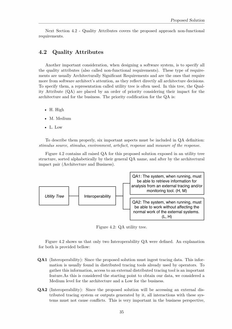
Proposed Solution
Next Section 4.2 - Quality Attributes covers the proposed approach non-functionalrequirements.
4.2 Quality Attributes
Another important consideration, when designing a software system, is to specify allthe quality attributes (also called non-functional requirements). These type of require-ments are usually Architecturally Significant Requirements and are the ones that requiremore from software architect’s attention, as they reflect directly all architecture decisions.To specify them, a representation called utility tree is often used. In this tree, the Qual-ity Attribute (QA) are placed by an order of priority considering their impact for thearchitecture and for the business. The priority codification for the QA is:
• H. High
• M. Medium
• L. Low
To describe them properly, six important aspects must be included in QA definition:stimulus source, stimulus, environment, artefact, response and measure of the response.
Figure 4.2 contains all raised QA for this proposed solution exposed in an utility treestructure, sorted alphabetically by their general QA name, and after by the architecturalimpact pair (Architecture and Business).
Utility Tree InteroperabilityQA2: The system, when running, mustbe able to work without affecting the
normal work of the external systems. (L, H)
QA1: The system, when running, mustbe able to retrieve information for
analysis from an external tracing and/ormonitoring tool. (H, M)
Figure 4.2: QA utility tree.
Figure 4.2 shows us that only two Interoperability QA were defined. An explanationfor both is provided bellow:
QA1 (Interoperability): Since the proposed solution must ingest tracing data. This infor-mation is usually found in distributed tracing tools already used by operators. Togather this information, access to an external distributed tracing tool is an importantfeature.As this is considered the starting point to obtain our data, we considered aMedium level for the architecture and a Low for the business.
QA2 (Interoperability): Since the proposed solution will be accessing an external dis-tributed tracing system or outputs generated by it, all interactions with these sys-tems must not cause conflicts. This is very important in the business perspective,
35

Chapter 4
because if our solution is not co-habitable with already used systems, it may becompletely rejected. For the architectural perspective it does not represent a bigimpact, and therefore a Low level was assigned.
4.3 Technical Restrictions
In this Section, technical restrictions considered in proposed solution are presented.
In software engineering, after specifying functional and non-functional requirementsfor a solution, comes the specification of business restrictions, however, in this projectnone were raised due to the fact that this work is focused on exploration and research.
To define the technical restrictions, we used an id and its corresponding description.Table 4.2 presents the technical restrictions considered for the proposed solution.
Table 4.2: Technical restrictions specification.
ID DescriptionTR-1 Use OpenTSDB as a Time-Series database.
Table 4.2 shows that we have raised only one technical restriction. This technicalrestriction was considered because Professor Jorge Cardoso, acting as a client for thissolution demanded it. OpenTSDB is the database that they are currently using in theirprojects at Huawei Research Center. This restriction will ease their work to introducechanges if needed.
4.4 Architecture
In this Section, the architecture is presented based on all previous topics with resourceto the defined Simon Brown’s C4 Model [59]. This approach of defining an architectureuses four diagrams: 1 - Context Diagram, 2 - Container Diagram, 3 - Component Diagramand 4 - Code Diagram. To define the architecture for our solution, only the first threerepresentations were considered. Every representation will be exposed with a explana-tion of the decisions taken to draw each diagram. After presenting the representationsand the corresponding explanations, we will cycle thought all architectural drivers: QA,business and technical restrictions, in order to explain where they are reflected and theconsiderations taken to produce this architecture.
4.4.1 Context Diagram
In this Subsection the context diagram is presented. This diagram allows us to see“the big picture” of the overall system as it represents the system as a “big box” and thecorresponding interactions with users and external software systems. Figure 4.3 presentsthe context diagram for this solution.
36
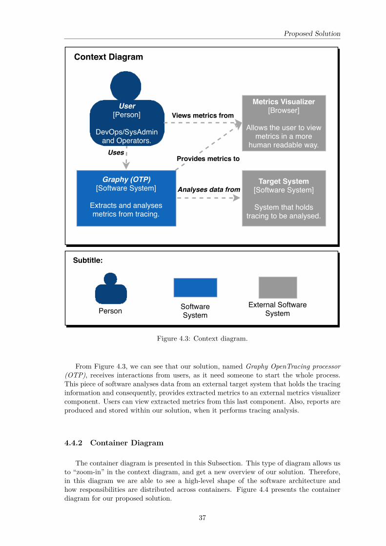
Proposed Solution
Context Diagram
Graphy (OTP)[Software System]
Extracts and analysesmetrics from tracing.
Uses
Subtitle:
PersonExternal Software
SystemSoftwareSystem
Target System[Software System]
System that holdstracing to be analysed.
User[Person]
DevOps/SysAdminand Operators.
Analyses data from
Metrics Visualizer[Browser]
Allows the user to viewmetrics in a more
human readable way.
Provides metrics to
Views metrics from
Figure 4.3: Context diagram.
From Figure 4.3, we can see that our solution, named Graphy OpenTracing processor(OTP), receives interactions from users, as it need someone to start the whole process.This piece of software analyses data from an external target system that holds the tracinginformation and consequently, provides extracted metrics to an external metrics visualizercomponent. Users can view extracted metrics from this last component. Also, reports areproduced and stored within our solution, when it performs tracing analysis.
4.4.2 Container Diagram
The container diagram is presented in this Subsection. This type of diagram allows usto “zoom-in” in the context diagram, and get a new overview of our solution. Therefore,in this diagram we are able to see a high-level shape of the software architecture andhow responsibilities are distributed across containers. Figure 4.4 presents the containerdiagram for our proposed solution.
37
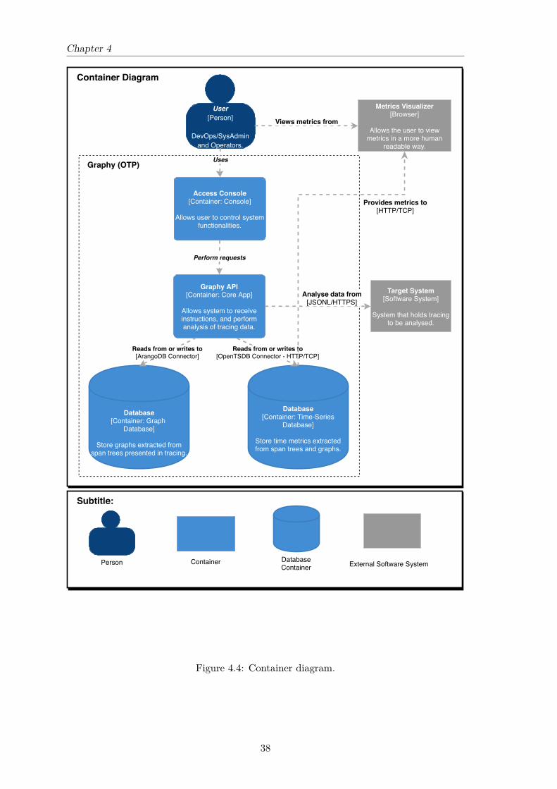
Chapter 4
Container Diagram
Graphy (OTP)
User[Person]
DevOps/SysAdminand Operators.
Uses
Target System[Software System]
System that holds tracingto be analysed.
Access Console[Container: Console]
Allows user to control systemfunctionalities.
Graphy API[Container: Core App]
Allows system to receiveinstructions, and performanalysis of tracing data.
Perform requests
Database[Container: Time-Series
Database]
Store time metrics extractedfrom span trees and graphs.
Database[Container: Graph
Database]
Store graphs extracted fromspan trees presented in tracing.
Subtitle:
Person External Software SystemContainer
Reads from or writes to[ArangoDB Connector]
Reads from or writes to[OpenTSDB Connector - HTTP/TCP]
Analyse data from[JSONL/HTTPS]
DatabaseContainer
Metrics Visualizer[Browser]
Allows the user to viewmetrics in a more human
readable way.
Text
Provides metrics to[HTTP/TCP]
Views metrics from
Figure 4.4: Container diagram.
38
Proposed Solution
Figure 4.4 contains the main containers involved in our solution. The first one, fromtop to bottom, is the Access Console and this container was considered as it is needed forthe user to be able interact with the Graphy Application Programming Interface (API).This last one controls the entire OpenTracing system, uses a communication protocol toretrieve tracing information from external target system, and two databases to store theinformation resulted from processing tracing data – a Graph Database (GDB) and a TimeSeries Database (TSDB). The second database provides metrics to be visualized in anexternal metrics visualizer system.
4.4.3 Component Diagram
This Subsection contains the last diagram, the component diagram. This type ofdiagram gives a more deeper vision about the system, and therefore, it reveals the maincomponents. Figure 4.5 presents the component diagram for this solution.
Figure 4.5 provides us with a lower level visualization of Graphy API container com-posed by eight components. At its core we have Graphy Controller, a component withthe responsibility of receiving requests from the user through Access Console and controlOpenTracing Processor, Tracing Collector and Data Analyser components. The first onehas the objective of mapping tracing data, span trees and service dependency graphs in-stantiation into memory. The second one collects tracing, the information that feeds thisentire application, from local files or from external systems, e.g., Zipkin. The last one,Data Analyser, identifies outliers presented in time-series metrics extracted from tracing,allowing our solution to detect anomalous services presented in distributed systems. GraphProcessor is the component for graphs handling, thus it has the capability of performingoperations over graphs, e.g., subtract one graph from another, extract node degrees andcount connections between nodes. The remaining components, Graphs Repository andMetrics Repository, are used to map graphs and time-series metrics, respectively, into andfrom their corresponding databases.
To check the architecture produced, we will now cycle between both QA and check werethey are reflected in the architecture presented for this solution, explaining the trade-offinvolved and what were our considerations about each one.
QA1 and QA2 are satisfied by the fact that the system is able to collect data froman external system. Using a communication protocol where data is exchanged thoughtHypertext Transfer Protocol (HTTP) and exposed API, allows to externally request littlechucks of data from target systems without interfering with their normal function.
Finally, for the only technical restriction raised, we can see that it is satisfied by theusage of OpenTSDB as the main TSDB for our solution.
This solution does not have many architectural drivers: quality attributes, businessconstraints and technical restrictions, due to being a prototype. The main objective is toproduce a solution capable of explore tracing data allowing us to conduct a research aboutwhat we can do with tracing, therefore it does not have many architectural constraints.Nevertheless, with the presentation of these four sections, we conclude that our solutionsatisfies all the architectural drivers, and therefore, we may claim that the proposed ar-chitecture fits our needs as a solution.
Next Chapter, 5 - Implementation Process, covers the implementation of the solutionpresented in the current chapter. All implemented algorithms and technical decisions arediscussed and explained in detail.
39
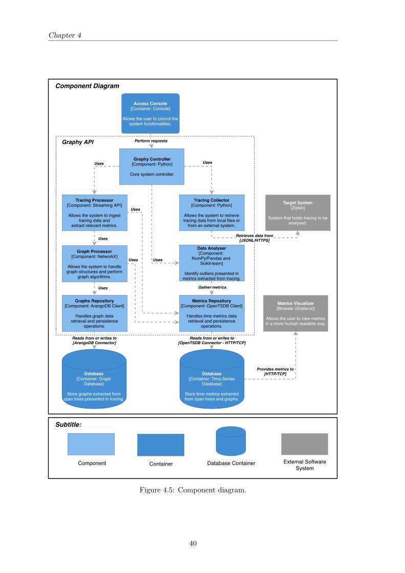
Chapter 4
Component Diagram
Graphy API
Target System[Zipkin]
System that holds tracing to beanalysed.
Access Console[Container: Console]
Allows the user to control thesystem functionalities.
Perform requests
Database[Container: Time-Series
Database]
Store time metrics extractedfrom span trees and graphs.
Database[Container: Graph
Database]
Store graphs extracted fromspan trees presented in tracing.
Subtitle:
External SoftwareSystem
Container
Reads from or writes to[ArangoDB Connector]
Reads from or writes to[OpenTSDB Connector - HTTP/TCP]
Retrieves data from[JSONL/HTTPS]
Database ContainerComponent
Uses
Graph Processor[Component: NetworkX]
Allows the system to handlegraph structures and perform
graph algorithms.
Tracing Processor[Component: Streaming API]
Allows the system to ingesttracing data and
extract relevant metrics.
Uses
Graphy Controller[Component: Python]
Core system controller.
Graphs Repository[Component: ArangoDB Client]
Handles graph dataretrieval and persistence
operations.
Uses Uses
Uses
Uses
Uses
Metrics Repository[Component: OpenTSDB Client]
Handles time metrics dataretrieval and persistence
operations.
Metrics Visualizer[Browser (Grafana)]
Allows the user to view metricsin a more human readable way.
Provides metrics to[HTTP/TCP]
Tracing Collector[Component: Python]
Allows the system to retrievetracing data from local files or
from an external system.
Data Analyser[Component:
NumPy/Pandas and Scikit-learn]
Identify outliers presented inmetrics extracted from tracing.
Gather metrics
Figure 4.5: Component diagram.
40
Chapter 5
Implementation Process
This Chapter presents the implementation process of the proposed solution explainedin previous Chapter. Three main sections are covered in this Chapter: Firstly, in Sec-tion 5.1 - Huawei Tracing Data Set, the data provided to perform this research is pre-sented and analysed. Secondly, in Section 5.2 - OpenTracing Processor Component, theimplementation of (OpenTracing processor (OTP)), our proposed solution to collect andstore metrics from tracing data is explained in detail with intermediate results. Finally,in Section 5.3 - Data Analysis Component, the approach and methods for analysis of thestored observations are presented.
5.1 Huawei Tracing Data Set
The starting point for this solution and every method developed within it was a dataset provided by Huawei, represented by professor Jorge Cardoso. To gain access to thisinformation, a NDA: Non-disclosure agreement was signed by both parts. This data setcontains the results of tracing data gathered from an experimental OpenStack cluster usedby the company for testing purposes, and covers two days of operation. Consequently, twofiles were provided, one for each day. These files were generated in 10 of July, 2018 and,for protection, some fields of the data set were obfuscated during the generation process.Table 5.1 contains some details about the provided data set.
Table 5.1: Huawei tracing data set provided for this research.
File Date 2018-06-28 2018-06-29Spans count 190 202 239 693Traces count 64 394 74 331
From Table 5.1, we can see some detail regarding spans and trace counting for eachday. Both files were written in JSONL format [60]. This file format is an extension tothe lightweight data-interchange standard JavaScript Object Notation (JSON): JavaScriptObject Notation, however, in JSONL format multiple JSON are separated by a new linecharacter. Each span is presented by a single JSON, therefore, each line contains a spanencoded in JSON format. To count spans a line count in each file was enough. To counttraces, spans must be mapped to span trees, and then the total of trees represent the tracecount. Algorithms to perform this conversion are presented further, in Section 5.2 - Open-Tracing Processor Component.
41

Chapter 5
Span data format is defined in an open source specification called OpenTracing [61],however, companies and software developers are not obliged to follow it, thus they canproduce their own span data format, leading to difficulties developing a general purposetool for tracing analysis. Therefore, to ease the interpretation of spans presented in thedata set, a file with instructions about the specification was provided. In this file, adefinition was given about possible fields and their corresponding data types. A sampleof the fields and their descriptions are exposed in Table 5.2.
Table 5.2: Span structure definition.
Field DescriptiontraceId Unique id of a trace (128-bit string).name Human-readable title of the instrumented function.timestamp UNIX epoch in milliseconds.id Unique id of the span (64-bit string).parentId Reference to id of parent span.duration Span duration in microseconds.binaryAnnotations protocol - “HTTP” or “function” for RPC calls;
http.url - HTTP endpoint;http.status_code - Result of the HTTP operation.
annotations value - Describes the position in trace (based on Zipkinformat). Could be one of the following values or other:“cs” (client send), “cr” (client receive), “ss” (server send)or “sr” (server receive);timestamp - UNIX epoch in microseconds;endpoint - Which endpoint generated a trace event.
Also, the file contained two notes. To point each one, has they are very important, wepresent them bellow.
1. Time units are not consistent, some fields are in milliseconds and some are in mi-croseconds.
2. Trace spans may contain more or less fields, except those mentioned here.
From Table 5.2, we get a notion about the fields that can be found in spans. Thesefields are defined by OpenTracing specification, therefore, is important that companiesfollows the specification, even if open source.
In this data set, spans are composed by: “traceId”, “name”, “timestamp”, “id”, “par-entId” and “duration”. These are the main required fields, because they represent thefoundations for tracing data, containing the identification, relation and temporal track ofthe span. Also, these fields are fixed, meaning that they are always represented by thedefined field name. The same can not be said from the remaining fields: “binaryAnno-tations” and “annotations”. These tow fields are always identified by these field names,however, their values are maps and therefore, have values stored in key - value pairs. Thisbrings some consistency problems and we might not know clearly what is available ina span, when working with it. As said in the second point presented in the list above:“Trace spans may contain more or less fields, except those mentioned here”, and for thisreason, there is a tremendous explosion in possibilities, because there might be keys withcorresponding values for some particular spans and it gets hard to generalise this in auniform span structure.
42
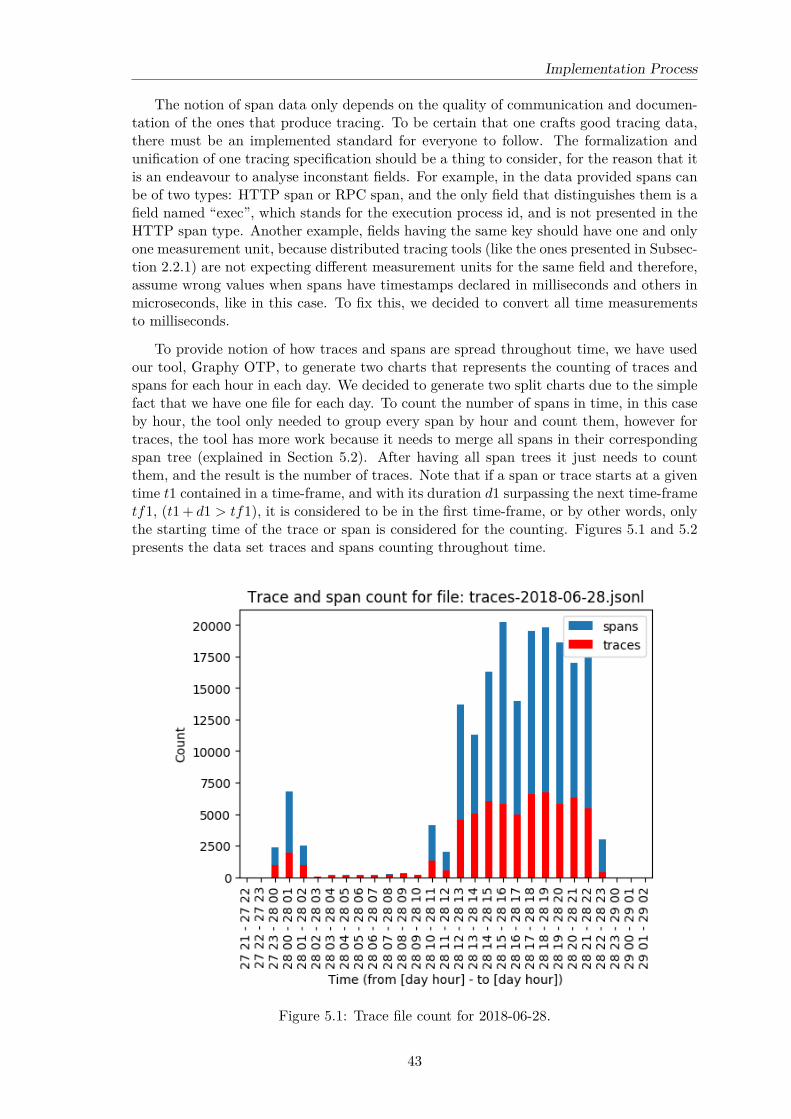
Implementation Process
The notion of span data only depends on the quality of communication and documen-tation of the ones that produce tracing. To be certain that one crafts good tracing data,there must be an implemented standard for everyone to follow. The formalization andunification of one tracing specification should be a thing to consider, for the reason that itis an endeavour to analyse inconstant fields. For example, in the data provided spans canbe of two types: HTTP span or RPC span, and the only field that distinguishes them is afield named “exec”, which stands for the execution process id, and is not presented in theHTTP span type. Another example, fields having the same key should have one and onlyone measurement unit, because distributed tracing tools (like the ones presented in Subsec-tion 2.2.1) are not expecting different measurement units for the same field and therefore,assume wrong values when spans have timestamps declared in milliseconds and others inmicroseconds, like in this case. To fix this, we decided to convert all time measurementsto milliseconds.
To provide notion of how traces and spans are spread throughout time, we have usedour tool, Graphy OTP, to generate two charts that represents the counting of traces andspans for each hour in each day. We decided to generate two split charts due to the simplefact that we have one file for each day. To count the number of spans in time, in this caseby hour, the tool only needed to group every span by hour and count them, however fortraces, the tool has more work because it needs to merge all spans in their correspondingspan tree (explained in Section 5.2). After having all span trees it just needs to countthem, and the result is the number of traces. Note that if a span or trace starts at a giventime t1 contained in a time-frame, and with its duration d1 surpassing the next time-frametf1, (t1+ d1 > tf1), it is considered to be in the first time-frame, or by other words, onlythe starting time of the trace or span is considered for the counting. Figures 5.1 and 5.2presents the data set traces and spans counting throughout time.
Figure 5.1: Trace file count for 2018-06-28.
43

Chapter 5
Figure 5.2: Trace file count for 2018-06-29.
Figure 5.1 presents the counting of traces and spans for the 28th of June, 2018. In thisFigure we can spot a “pit” in quantity from 2AM to 10AM. No explanation for this wasgiven, however, at this point we assumed that extracting metrics from data in this timeinterval would produce less points, thus less resolution. This is visible in metrics presentedin Figure 5.3, reproduced using Grafana. The quantity of data for the rest of the day issomehow inconstant, however, there is no lack of data like in the previous day.
Figure 5.2 presents the counting of traces and spans for the 28th of June, 2018. In thisFigure there are no “pits”, and consequently, the quantity of information is more constantthroughout time.
To summarise, this system produces an average of 5000 traces an hour and 15000 spansan hour. Also, the quantity of information provided in the second day (29th of June) ismore constant, and therefore, better for analysis, than in the first day (28th of June).Nevertheless, this data set has sufficient information to study tracing data and developmethods for tracing data, and then, it is a suitable data set for this research project.
Next Chapter, 5.2 - OpenTracing Processor Component, covers the explanation andalgorithms used over this data set for tracing metrics extraction and quality analysis. Also,some visualizations of metrics extracted from tracing data are provided.
44

Implementation Process
5.2 OpenTracing Processor Component
In this Chapter, the implementation for the first component of the proposed solution,OTP, is presented and explained, hence, functional requirements defined in Table 4.1, ser-vice dependency graph handling, span trees generation and methods for metrics extractionand storing from tracing data will be covered.
Starting by the first two functional requirements (FR-1 to FR-2). These require com-munication with distributed tracing tools, to obtain tracing data and to retrieve servicedependency graphs. We have decided to use Zipkin, as a distributed tracing tool forholding our data set, instead of Jaeger only due to simplicity in setup configuration. Tosetup this tool a Docker container was instantiated in an external server. Communica-tion methods are implemented in Tracing Collector component. To feed information toour solution, one can use two ways: collect tracing data from local files, or export themto Zipkin and ingest it through HTTP requests. This configurations can be changed byediting a configuration file provided with the solution. The configurations to edit are filelocations in local machine and Zipkin IP (Internet Protocol) address.
After collecting information from one of the two defined sources by Tracing Collector,data is passed to Tracing Processor which ingests and maps all the information into inmemory data structures. Data can be either trace data or service dependency graphs. If itis a graph, it is transferred to Graph Processor for process, graph metrics extraction andlater storage, otherwise, it is processed in Tracing Processor to extract defined metricsfrom tracing. The algorithm for metrics extraction from tracing and service dependencygraphs is presented at a high abstraction level in Algorithm 1.
Algorithm 1: Algorithm for metrics extraction from tracing.Data: Trace files/Trace data.Result: Trace metrics written in the time-series database.
1 Connect to Time-Series database;2 Read time_resolution, start_time and end_time from configuration;3 Read traces from trace files/trace data;4 Post traces to Zipkin;5 Get services from Zipkin;6 Calculate time_intervals using start_time, end_time and time_resolution;7 while time_interval in time_intervals do8 Get service_dependencies from Zipkin;9 Build service_dependency_graph using service_dependencies;
10 Extract graph_metrics from service_dependency_graph;11 while service in services do12 Get traces from Zipkin;13 Map traces in SpanTrees;14 Extract service_metrics from SpanTrees;15 Post graph_metrics to Time-Series database;16 Post service_metrics to Time-Series database;
Algorithm 1 contains some core functionalities implemented in components presentedin OTP solution. This algorithm aims for metrics extraction from tracing data and performthis procedure using two main data structures: service dependency graphs and tracing datamapped into SpanTrees.
45
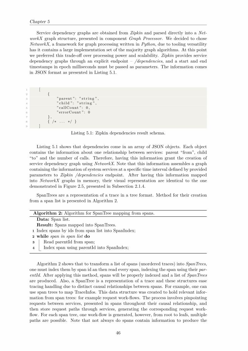
Chapter 5
Service dependency graphs are obtained from Zipkin and parsed directly into a Net-workX graph structure, presented in component Graph Processor. We decided to choseNetworkX, a framework for graph processing written in Python, due to tooling versatilityhas it contains a large implementation set of the majority graph algorithms. At this pointwe preferred this trade-off over processing power and scalability. Zipkin provides servicedependency graphs through an explicit endpoint – /dependencies, and a start and endtimestamps in epoch milliseconds must be passed as parameters. The information comesin JSON format as presented in Listing 5.1.
1 [2 {3 ” parent ” : ” s t r i n g ” ,4 ” ch i l d ” : ” s t r i n g ” ,5 ” cal lCount ” : 0 ,6 ” errorCount ” : 07 } ,8 { /∗ . . . ∗/ }9 ]
Listing 5.1: Zipkin dependencies result schema.
Listing 5.1 shows that dependencies come in an array of JSON objects. Each objectcontains the information about one relationship between services: parent “from”, child“to” and the number of calls. Therefore, having this information grant the creation ofservice dependency graph using NetworkX. Note that this information assembles a graphcontaining the information of system services at a specific time interval defined by providedparameters to Zipkin /dependencies endpoint. After having this information mappedinto NetworkX graphs in memory, their visual representation are identical to the onedemonstrated in Figure 2.5, presented in Subsection 2.1.4.
SpanTrees are a representation of a trace in a tree format. Method for their creationfrom a span list is presented in Algorithm 2.
Algorithm 2: Algorithm for SpanTree mapping from spans.Data: Span list.Result: Spans mapped into SpanTrees.
1 Index spans by ids from span list into SpanIndex;2 while span in span list do3 Read parentId from span;4 Index span using parentId into SpanIndex;
Algorithm 2 shows that to transform a list of spans (unordered traces) into SpanTrees,one must index them by span id an then read every span, indexing the span using their par-entId. After applying this method, spans will be properly indexed and a list of SpanTreesare produced. Also, a SpanTree is a representation of a trace and these structures easetracing handling due to distinct causal relationships between spans. For example, one canuse span trees to map TraceInfos. This data structure was created to hold relevant infor-mation from span trees: for example request work-flows. The process involves pinpointingrequests between services, presented in spans throughout their causal relationship, andthen store request paths through services, generating the corresponding request work-flow. For each span tree, one work-flow is generated, however, from root to leafs, multiplepaths are possible. Note that not always do spans contain information to produce the
46
Implementation Process
path, and therefore, some request paths are dubious, depending only on the completenessquality of tracing. The method to produce request work-flows is described in Algorithm 3.
Algorithm 3: Work-flow type algorithm.Data: Trace files/Trace data.Result: Comma-separated values (CSV) with unique work-flow types, their
corresponding count and times.1 Read start_time and end_time from configuration;2 Read SpanList from trace files/trace data within defined time_frame;3 while have Spans in SpanList do4 Read Span;5 Map Span to SpanTrees;6 while have SpanTree in SpanTrees do7 Read SpanTree;8 Map SpanTree to TraceInfos;9 Read TraceInfo;
10 Read work-flows, work-flow count, times, (others) from TraceInfo;11 Write fields to CSV files;
The method described in Algorithm 3 aims to use tracing to produce span trees, andthen generate TraceInfos to retrieve request work-flow paths.
These two data structures, service dependency graphs and span trees, are the founda-tions to extract metrics from tracing data, satisfy the functional requirements presentedin Section 4.1 and answer the final research questions defined in Section 3.2.
The metrics that OTP is able to extract from tracing data, for a defined time interval,are the following:
1. Number of incoming/outgoing service calls;
2. Average response time by service;
3. Service connection, i.e., other services invoking and being invoked by the system,i.e., the service dependency graph variation.
4. Service degree (in/out/total);
5. Service HTTP status code ratio. (sum of success or failure count over total statuscode count)
These metrics are all related with time and represent observations of values extractedfrom tracing data, therefore, as time-series metrics they are stored in a Time SeriesDatabase (TSDB). Explanation of used technology and procedure is provided later onthis Section.
Table 5.3 relates each metric with a functional requirement, and correspondent finalresearch question. Functional requirements are identified by an id from Table 4.1.
47

Chapter 5
Table 5.3: Relations between final research questions, functional requirements and metrics.
ResearchQuestion
FunctionalRequirements
Metrics
1. Is there anyanomalous service?
FR-5;FR-5;FR-6.
Number of incoming service calls;Number of outgoing service calls;Average response time by service.
2. What is the over-all reliability of theservice?
FR-7;FR-8.
No metric extracted;Service HTTP status code ratio.
3. Which serviceconsumes more timewhen consideringthe entire set ofrequests?
FR-9;FR-10.
Service degree;Service dependency graph variation.
For Table 5.3, only functional requirements from numbers 5 to 10 were considered, dueto being the ones related with metrics extraction. As said before, only question number 1was considered for metrics extraction. The remaining, defined at grey colour, were imple-mented and OTP extracts them, however, they were not further analysed in this research.Almost all functional requirements have one metric associated except one, FR-7. Thisfunctional requirement was implemented, and our solution allows to generate work-flowpaths from tracing data, however, no metric was defined. Nevertheless, the implementationof this functionality helped us understanding results for the first final research question –Method for work-flow generation from tracing data is explained Algorithm 3.
Span trees are a representation of causal relationship between spans. Two types of timebased metrics are extracted from span trees: 1. Average response time by service in time;and 2. Service HTTP status code ratio in time. To extract the first metric type, durationand annotations/endpoint/serviceName values presented in spans , when defined, are usedto calculate the average response time by service. For each span tree a list of services andtheir corresponding average times are obtained. After gathering all values from every spantree presented in the defined time-frame, the values are merged and posted to the TSDB.The second metric, is extracted through a calculation of status codes ratio by each service.For this, binaryAnnotations/http.status_code and annotations/endpoint/serviceName val-ues are used. Also, equally to the previous metric, values are merged and posted to theTSDB.
Service dependency graphs are a representation of dependencies of services at a specifictime-frame. Three types of time based metrics are extracted from service dependencygraphs: 1. Number of incoming/outgoing service calls in time; 2. Entry/exit of servicesin time (service dependency graph node variation); and 3. Service degree (in/out/total)in time. To extract the first metric type, the values in between (Edges) services (Nodes)are retrieved. These values are dispatched for storage with service name, flow indication(incoming/outgoing), timestamp and number of calls. The second metric type is extractedhaving two successive graphs and performing their difference. For example, if GraphA hasnodes A,B,C and GraphB, nodes A,C,D,E, the difference between them will result intwo service entries D,E and one exit. Last metric type, service degree, is extractedby retrieving the number of connections from each service. For example, consider thatGraphC has a service A connected from itself to services B,C,D. In this graph, serviceA has an out degree of three and an in degree of zero. The remaining services have an outdegree of zero and an in degree of one. Methods to extract these metrics are implemented
48

Implementation Process
in Graph Processor and resource to NetworkX to handle graph structures. All thesemetrics are then posted to the TSDB.
At this point, our solution is able to retrieve and store time-series metrics from tracingdata. For the TSDB, we have decided to use OpenTSDB, due to technical restrictionsimposed in Section 4.3. There was a client implementation for usage in Python, however,the support was not good due to lack of updates and clear documentation. For this reason,we decided to implement our own OpenTSDB client in Python using their ApplicationProgramming Interface (API) specification, – Metrics Repository component. Later, whenall implementation from tracing collection through trace metrics storage in the TSDB, weused a browser metrics visualizer. To do this, a Docker container with Grafana, a datavisualization tool capable of rendering time-series metrics in charts and present themin dashboards. The decision to use this tool, was due to easy to setup and integratedcompatibility with our TSDB. We just needed to create a container and, through a urlconfiguration in Grafana, we established a link to the TSDB.
Figures 5.3, 5.4, 5.5, and 5.6, contain sample representations of extracted time-seriesmetrics stored in our TSDB.
06-28 0006-28 04
06-28 0806-28 12
06-28 1606-28 20
06-29 0006-29 04
06-29 08
Time (Month-Day Hour)
0
10
20
30
40
Num
ber o
f inc
oming
calls
Service A Calls [Incoming]
06-28 0006-28 04
06-28 0806-28 12
06-28 1606-28 20
06-29 0006-29 04
06-29 08
Time (Month-Day Hour)
0
500
1000
1500
Tota
l valu
e
Service A Calls [Total]
06-28 0006-28 04
06-28 0806-28 12
06-28 1606-28 20
06-29 0006-29 04
06-29 08
Time (Month-Day Hour)
0
500
1000
1500
Out v
alue
Service A Calls [Outgoing]
06-28 1206-28 15
06-28 1806-28 21
06-29 0006-29 03
06-29 0606-29 09
Time (Month-Day Hour)
0
50
100
150
200
Num
ber o
f inc
oming
calls
Service B Calls [Incoming]
06-28 1206-28 15
06-28 1806-28 21
06-29 0006-29 03
06-29 0606-29 09
Time (Month-Day Hour)
0
50
100
150
200
Tota
l valu
e
Service B Calls [Total]
06-28 1206-28 15
06-28 1806-28 21
06-29 0006-29 03
06-29 0606-29 09
Time (Month-Day Hour)
0
5
10
15
20
25
Out v
alue
Service B Calls [Outgoing]
06-28 0006-28 04
06-28 0806-28 12
06-28 1606-28 20
06-29 0006-29 04
06-29 08
Time (Month-Day Hour)
0
100
200
300
Num
ber o
f inc
oming
calls
Service C Calls [Incoming]
06-28 0006-28 04
06-28 0806-28 12
06-28 1606-28 20
06-29 0006-29 04
06-29 08
Time (Month-Day Hour)
0
100
200
300
400
Tota
l valu
e
Service C Calls [Total]
06-28 0006-28 04
06-28 0806-28 12
06-28 1606-28 20
06-29 0006-29 04
06-29 08
Time (Month-Day Hour)
0
5
10
15
20
25
30
Out v
alue
Service C Calls [Outgoing]
Figure 5.3: Service calls samples.
06-28 0006-28 04
06-28 0806-28 12
06-28 1606-28 20
06-29 0006-29 04
06-29 08
Time (Month-Day Hour)
0
2
4
6
8
10
12
Gain
val
ue
Service dependency variation [Gain]
06-28 0006-28 04
06-28 0806-28 12
06-28 1606-28 20
06-29 0006-29 04
06-29 08
Time (Month-Day Hour)
2
0
2
4
6
8
10
12
Tota
l val
ue
Service dependency variation [Total]
06-28 0006-28 04
06-28 0806-28 12
06-28 1606-28 20
06-29 0006-29 04
06-29 08
Time (Month-Day Hour)
0.0
0.5
1.0
1.5
2.0
2.5
3.0
Loss
val
ue
Service dependency variation [Loss]
Figure 5.4: Service dependency variation samples.
49

Chapter 5
06-28 00
06-28 04
06-28 08
06-28 12
06-28 16
06-28 20
06-29 00
06-29 04
06-29 08
Time (Month-Day Hour)
1
2
3
4
5
Resp
onse
Tim
e (
1e5
mill
iseco
nd
s)Service A Average Response Time
06-28 12
06-28 15
06-28 18
06-28 21
06-29 00
06-29 03
06-29 06
06-29 09
Time (Month-Day Hour)
0.5
1.0
1.5
2.0
2.5
3.0
3.5
4.0
4.5
Resp
onse
Tim
e (
1e6
mill
iseco
nd
s)
Service B Average Response Time
06-28 00
06-28 04
06-28 08
06-28 12
06-28 16
06-28 20
06-29 00
06-29 04
06-29 08
Time (Month-Day Hour)
0
1
2
3
4
5
Resp
onse
Tim
e (
1e6
mill
iseco
nd
s)
Service C Average Response Time
Figure 5.5: Service average response time samples.
06-28 0006-28 04
06-28 0806-28 12
06-28 1606-28 20
06-29 0006-29 04
06-29 08
Time (Month-Day Hour)
0.0
0.2
0.4
0.6
0.8
1.0
Ratio
Service A Request Status code ratios2XX4XX5XX
06-28 1206-28 15
06-28 1806-28 21
06-29 0006-29 03
06-29 0606-29 09
Time (Month-Day Hour)
0.0
0.2
0.4
0.6
0.8
1.0
Ratio
Service B Request Status code ratios
2XX4XX
06-28 0006-28 04
06-28 0806-28 12
06-28 1606-28 20
06-29 0006-29 04
06-29 08
Time (Month-Day Hour)
0.0
0.2
0.4
0.6
0.8
1.0
Ratio
Service C Request Status code ratios
2XX4XX5XX
Figure 5.6: Service status code ratio samples.
Figure 5.3 represent samples about the number of service request calls metric. Inthis Figure, we have 9 plots, three in each row, representing three variations (incoming,outgoing and total) of this metric for one service. In this metric we can clearly see thelack of information presented in tracing for the beginning of the first day.
Figure 5.4 contain samples about service dependency variation, one for each metric(gain, loss and total). Total are the result of gain− loss. Gain stands for the number ofnew service entries in system, and loss, represent the number of service exits in system.
Last Figure, 5.6, shows the gathering of status code ratio samples for three distinctservices. The ratio varies from 0.0 to 1.0, and represent the proportion of status codegroups (2xx – Success, 4xx – Client error and 5xx – Other errors).
Also, service dependency graphs are stored for further access after being processed byGraph Processor component. We have decided to use ArangoDB as our Graph Database(GDB). This decision was based in the “Multi data-type support” provided by this database,allowing us to extend our graph structures to whatever we wanted, enhancing our graphstorage possibilities and relieving the implementation from parsing data-types. Thisdatabase has a Python client, pyArango [62], which revealed lack of features, leadingto propositions for functionality creation and issue declarations in GitHub. However, theanswers were not pleasant due to lack of support and people to maintain the project [63].This have lead to some difficulties when implementing Graphs Repository component inOTP. Difficulties from storing graphs with custom names to custom graph retrieval werefelted. The solution was to fork the project, perform changes and use our custom pyArangoclient. This changes were committed for review to the original project. We could not mit-igate these problems in advance because they were only perceived when using the client.
After presenting the first component, OTP, from our proposed solution, next Sec-tion 5.3 - Data Analysis Component covers the implementation of the second componentpresented in our solution.
50

Implementation Process
5.3 Data Analysis Component
In this Section, the implementation of the second component presented in our pro-posed solution, “Data Analysis” component, is presented and expected outcomes fromeach analysis are discussed.
“Data Analysis” component has the main objective of detecting anomalies, presentedin services, using time-series metrics extracted from tracing data using the componentpresented in previous Section and perform tracing quality analysis.
In our implementation, this component is detached from the remaining components,however, in architectural terms we have decided to place it has being part of the overallsolution. This is because there is nothing preventing total integration with other compo-nents presented in the solution. The reason to implement these methods detached fromthe remaining, was to ease our research path and increase flexibility. This means that,to ease our data exploration, implement these methods in Notebooks detached from theoverall components, allowed us to change code effortlessly and conceded focus on methodsdevelopment. Jupyter Notebook [64] was the notebook chosen for method implementation,hence, one server was created to hold our implementations in notebooks.
In this case, extracted time-series data belong to unlabelled data group. Data canbelong to unlabelled or labelled groups. Unlabelled data are information sampled from ofnatural, or human-created artefacts, that one can obtain from observing and record values.In this group, there is no “explanation” for each piece of data, as it just contains the data,and nothing else. Labelled data typically takes a set of unlabelled data and augmentseach piece of data with some sort of meaningful “tag”, “label”, or “class” that is somehowinformative or desirable to know. For example, for this solution, having labelled datawould help in identifying anomalies presented in our data set. However, only unlabelleddata was provided, and therefore, we needed to work with unlabelled data and performanomaly detection with it [65].
So, the approach was to use processed data produced from OTP, and perform theanalysis using “Data Analysis” component to point out service problems and performtracing quality analysis, as defined in Figure 4.1, to answer questions defined in Chapter 3:
1. Is there any anomalous behaviour in the system? (If yes, where?);
2. How can we measure the quality of tracing?
To answer the first question, using our proposed solution, one must use metrics ex-tracted from tracing data, namely the number of incoming / outgoing requests and theaverage response time for each service. These metrics are time-series metrics, and there-fore, anomaly detection using unsupervised learning algorithms are the way to do it [25].Metrics were obtained using methods defined in our OpenTSDB client, implemented inMetrics Repository component.
After extracting these metrics, they are allocated in a data structure called dataframefrom Pandas, an open source library that provides high-performance, easy-to-use datastructures and data analysis tools. This library was chosen due to being one of the mostused and popular for this purpose [66] – data science and data analysis. A Dataframe isa two-dimensional size-mutable, potentially heterogeneous tabular data structure withlabelled axes (rows and columns). In these data structures, values from time-seriesmetrics were stored in columns: timestamp (index), datetime, number_of_incoming_re-
51

Chapter 5
quests, number_of_outgoing_requests and average_response_time. In the end, a list ofdataframes are created, one dataframe for each service.
Before performing an analysis to detect if there are outliers presented in our data, theinformation must be checked and tested to verify if data have missing values. This is donebecause metrics are extracted from multiple sources and thus generates missing values.For example, we may have missing information for one of the three features in a row ofone dataframe. Missing values are a pain in data analysis and are represented by NaN indataframes, and for this reason,one can not apply anomaly detection algorithms over datawith missing values. To fulfil missing information there are two approaches:
1. Remove rows with missing values, which degrades the overall data and may resultin insufficient data;
2. Impute missing values, however, it may be dangerous because it introduces ”wrong”observations.
We decided to impute missing values because there were too keep information quantity.However, there are multiple ways for imputation of missing values into time-series data,depending on factors of trend and seasonality. Trending is the increasing or decreasingvalue in the series, and seasonality is the repeating short-term cycle in the series [25].Figure 5.7 shows the path to chose the correct method to fulfil information in time-seriesdata.
So, before applying the method, our component tests the data to chose the correctmethod to fulfil data. Figure 5.8 contains trend and seasonality sample tests performedover our data.
Figure 5.8 shows that there are clearly trends in our data, however, no seasonality wasdetected. For this reason, the selected method to fulfil data presented in dataframes isLinear Interpolation – Figure 5.7.
These dataframes are then processed by an unsupervised learning algorithm to detectif there are outliers. For the unsupervised learning algorithm there were: Isolation Forestsand OneClassSVM [68]. The first one uses binary decision trees to isolate data points andidentify outliers presented in the data set, the second one, generates density areas usingmax-margin methods, i.e. they do not model a probability distribution, hence the ideais to find a function that is positive for regions with high density of points, and negativefor small densities, identifying outliers presented in data. Figure 5.9 displays the errorcomparison of these two methods.
52

Implementation Process
Figure 5.7: Methods to handle missing data [67].
0
1x10e6
Tre
nd
Time
Trend and seasonality for time-series metric B
0
2000
Tre
nd
0.05
0.00
0.05
Seaso
nal
Time
Trend and seasonality for time-series metric A
0.05
0.00
0.05
Seaso
nal
Figure 5.8: Trend and seasonality results.
53

Chapter 5
Figure 5.9: Isolation Forests and OneClassSVM methods comparison [69].
From Figure 5.9, isolation forests prove to be a better method for outlier detectionbecause, from this test, it resulted in fewer errors as it did not construct a parametricrepresentation of the search space. For this reason, we decided to use Isolation Forests, todetect and identify outliers presented in time-series metrics extracted from tracing data.To implement Isolation Forests method we used Scikit-Learn, a library full of simple andefficient tools for data mining, data analysis and machine learning. All configurationsused from this library to implement Isolation Forests were setted to default. Therefore,Algorithm 4 presents the whole process to identify anomalous services presented in thesystem.
Algorithm 4: Anomalous service detection algorithm.Data: Processed data from tracing using OTP.Result: Report, in CSV file, containing identified anomalous services and
correspondent times.1 Read start_timestamp, end_timestamp, db_settings from configuration;2 Connect to TSDB;3 Retrieve metrics from TSDB using database connection, start_timestamp and
end_timestamp;4 Create dataframes with metrics data;5 Perform data imputation over dataframes;6 Feed Isolation Forests with metric columns from dataframes;7 Fire Isolation Forests method (Adds new column “anomaly” with -1 “Anomalous”
or 1 “Non-anomalous”);8 Filter “anomaly” column with -1 values from dataframes into
anomalous_dataframes;9 Write report with anomalous service names and times from
anomalous_dataframes data;
Algorithm 4 contains all the process explained above. The final outcome from thisalgorithm is a report containing all anomalous services and correspondent times identified.Also, later we decided to study further the pattern observed in anomalous regions. Forthis, the approach was to use the algorithm defined in 3 to analyse what happens towork-flows in “anomalous” and “non-anomalous” regions.
To answer the second question, it requires to perform a structural and time coverageanalysis. For the first analysis, the approach is to define a specification schema based onOpenTracing open source specification. This schema aims to test span structures in orderto detect structural problems present in spans, e.g., missed fields, wrong data types, typospresented in structure. The method implemented is presented in Algorithm 5.
54

Implementation Process
Algorithm 5: Span structure analysis algorithm.Data: Trace files/Trace data.Result: CSV file reporting span structure analysis.
1 Read specification from open_tracing_specification_schema.json;2 while not end of tracing do3 Read Span;4 Check Span against specification;5 Write results from “Check” to CSV file;
As we can see in Algorithm 5, our method aims to produce a report containing theresults of span structural analysis. To do this, first it needs to read the OpenTracingspecification schema. This schema is written in a JSON file, where the fields are annotatedwith tags: required, data-type: <string, int, other> and others. JSON Schema [70] wasthe library used to verify if each span complies with the specification. For the secondanalysis, the approach is to use spans presented in trace data to analyse the coverage ofeach trace. Figure 5.10 presents an example for time coverage in a trace.
Span A (duration 100ms)
Span B (duration 50ms)
Span C (duration 10 ms)
Time
Figure 5.10: Trace time coverage example.
Figure 5.10 gives us an example in which we have a trace with a root span of 100milliseconds of duration, and this root span has two children spans, one with 50ms, theother one with 10ms, the entire trace has a coverage of (50+10)/100 = 60%. This methodis applied to every trace, and the results are the stored in a CSV file to be plotted forvisualisation. In this case we apply it and split the results by service, with the objectiveof perceive the time coverability of tracing in each service. The method is presented inAlgorithm 6.
Algorithm 6: Trace coverability analysis algorithm.Data: Trace files/Trace data.Result: CSV file for each service reporting the coverability analysis.
1 Read start_time and end_time from configuration;2 Get services from Zipkin;3 while service in services do4 Get traces from Zipkin using service, start_time and end_time;5 Map traces in SpanTrees;6 Calculate trace_coverability using SpanTrees;7 Write trace_coverability to CSV file;
Algorithm 6 uses SpanTrees to calculate trace_coverability, this is due to causal re-lationships presented in these trees. As explained above, through Figure 5.10, one musthave a trace mounted in span relationships (span trees), to know when a span is child
55

Chapter 5
of another, and be able to calculate the coverability presented in a trace. This methodperforms this calculation for every service and, in the end, stores information about tracecoverability into a CSV file. This file is later used to produce plots about the service tracecoverability. What is expected from this method is that we achieve a plotting, where everyservice has a counting of traces that cover a certain amount of time.
To summarise, this tools gathers processed data and time-series data from our TSDB,extracted using OTP from original trace information. Then it perform data imputationto solve missing values problems, analyses resulting data using Isolation Forests, an un-supervised multiple feature machine learning algorithm, to identify outliers presented inour extracted metrics, and therefore, detect anomalies presented in services, identifyingtheir occurrences in time. Also, this tools uses tracing to perform an analysis about thestructure of spans presented in tracing, and uses processed data from OTP, to perform ananalysis of time coverage provided by tracing data.
Next Chapter 6, we will cover results obtained by this component, discuss these resultsand present OpenTracing data limitations.
56
Chapter 6
Results, Analysis and Limitations
In this Chapter we present the final results gathered from the “Data Analysis” com-ponent presented in Chapter 4 - Proposed Solution, to answer the questions defined inSection 3.2. Results for both questions, “1. Is there any anomalous service?” and “2. Howcan we measure the quality of tracing?”, are presented as well as a brief discussion regard-ing both results in Sections 6.1 and 6.2 respectively. Later, in the end of this Chapter, inSection 6.3, we explore some limitations regarding the OpenTracing data.
6.1 Anomaly Detection
For the first question, the approach was to use the OpenTracing processor (OTP)tool to extract metrics from tracing data to further analyse it using the unsupervisedlearning algorithm. The implemented algorithm used for metrics extraction is presentedin Algorithm 1.
After extract metrics, a tool for metrics visualisation (e.g., Grafana) was used to visu-alise metrics from OpenTSDB database. Samples from these visualizations were presentedin Figures 5.3, 5.4, 5.5 and 5.6. Therefore, the method explained in Algorithm 4 was ap-plied to metrics extracted from tracing data. From this algorithm, a Comma-separatedvalues (CSV) file is generated containing candidates to “possible anomalous regions” foreach service presented in the system. Figure 6.1 shows a sample of the result of outliersidentified in time-series data for a given hypothetical service.
57

Chapter 6
010
0030
000
1000
2000
010
0000
0
1530140000 1530160000 1530180000 1530200000 1530220000
05
10
Inco
min
g R
eque
sts
Out
goin
g R
eque
sts
Res
pons
e T
ime
(ms)
Gra
ph C
hang
es
Time Stamp
Figure 6.1: Sample of detection, using multiple feature, of “Anomalous” and“Non-Anomalous” time-frame regions for a service.
58

Results, Analysis and Limitations
Figure 6.1 contains a set of vertical red lines representing the points of identifiedanomalies in time, involving the three distinct time-series metrics. From this outlierdetection, using Isolation Forests, plots containing candidates to “possible anomalousregions” were generated. The outcome expected from these plots, were a clustering ofvalues in normal (“non-anomalous”) time-frame regions against clustering of values withoutliers scattered in distant regions (“anomalous”).
Figure 6.2 provides a representation of two time-frame samples, one for the “anoma-lous” region, and the other for the “non-anomalous” region considering the same service.In these samples we retrieved data to analyse and give answers to the first question. Forthis, we considered three features (as shown in the samples bellow): the number of incom-ing requests, the number of outgoing requests and the average response time. The sampleresolution for the time-frame is 10 minutes centred in a given timestamp.
Figure 6.2: Comparison between “Anomalous” and “Non-Anomalous” service time-frameregions.
As we can see in Figure 6.2, there is a clear difference between anomalous and non-anomalous regions. There is a drastic change in the range of values between the anomalousand non-anomalous regions, where the maximum for each feature changes greatly andtherefore, outliers are visible and evident in the observations. In the anomalous samples,it is possible to notice a clear crowding of points near the origin point of the chart andsome outliers in the upper-left and down-right regions of the chart. On the other side, inthe non-anomalous samples, all that is possible to notice is the crowding of points nearthe origin point of the chart. The crowding of points is what is expected to be the normalbehaviour for services, which means that is expected that the service can handle the loadwith good response times. Furthermore, after this observations, what is expected is toinvestigate what these points represent and what is causing this unexpected increment inthe number of incoming/outgoing requests and the average response time.
59
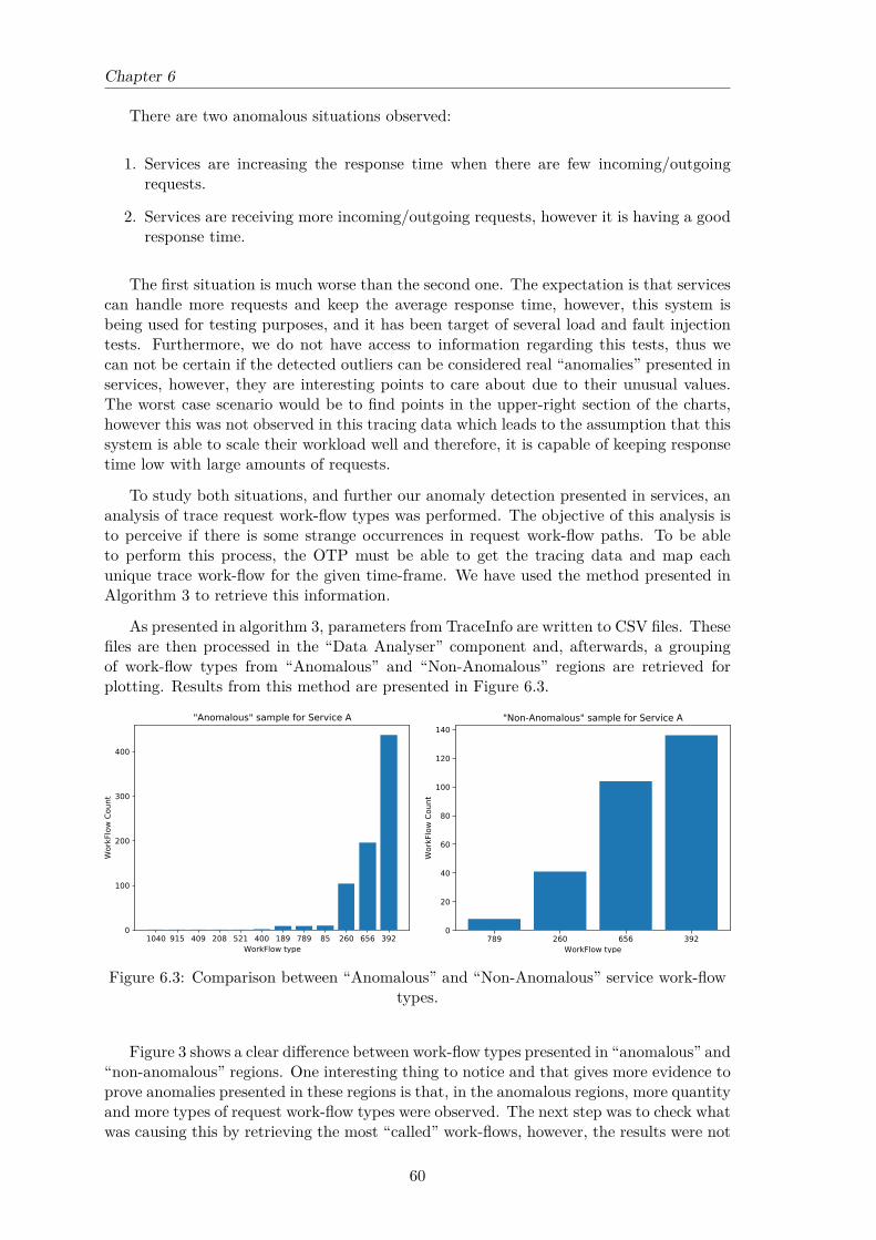
Chapter 6
There are two anomalous situations observed:
1. Services are increasing the response time when there are few incoming/outgoingrequests.
2. Services are receiving more incoming/outgoing requests, however it is having a goodresponse time.
The first situation is much worse than the second one. The expectation is that servicescan handle more requests and keep the average response time, however, this system isbeing used for testing purposes, and it has been target of several load and fault injectiontests. Furthermore, we do not have access to information regarding this tests, thus wecan not be certain if the detected outliers can be considered real “anomalies” presented inservices, however, they are interesting points to care about due to their unusual values.The worst case scenario would be to find points in the upper-right section of the charts,however this was not observed in this tracing data which leads to the assumption that thissystem is able to scale their workload well and therefore, it is capable of keeping responsetime low with large amounts of requests.
To study both situations, and further our anomaly detection presented in services, ananalysis of trace request work-flow types was performed. The objective of this analysis isto perceive if there is some strange occurrences in request work-flow paths. To be ableto perform this process, the OTP must be able to get the tracing data and map eachunique trace work-flow for the given time-frame. We have used the method presented inAlgorithm 3 to retrieve this information.
As presented in algorithm 3, parameters from TraceInfo are written to CSV files. Thesefiles are then processed in the “Data Analyser” component and, afterwards, a groupingof work-flow types from “Anomalous” and “Non-Anomalous” regions are retrieved forplotting. Results from this method are presented in Figure 6.3.
Figure 6.3: Comparison between “Anomalous” and “Non-Anomalous” service work-flowtypes.
Figure 3 shows a clear difference between work-flow types presented in “anomalous” and“non-anomalous” regions. One interesting thing to notice and that gives more evidence toprove anomalies presented in these regions is that, in the anomalous regions, more quantityand more types of request work-flow types were observed. The next step was to check whatwas causing this by retrieving the most “called” work-flows, however, the results were not
60

Results, Analysis and Limitations
good because of the completeness of the tracing data. The flows were not relevant tofurther our analysis because they were just calls from point A to point B, or representeda not so interesting request path due to involved services. Also, in some of these requestswork-flow path, high values of response time were observed and therefore, they tockedlonger to execute, however, like for the previous explanation, their path was not relevantto study. For these reasons, there were no possibility to extend our analysis and identifythe root cause for these abnormal observed behaviours. Therefore, at this point and forthis question, it is possible to say that this data set was exhaustively analysed, and animprovement of the tracing data, or the gathering of other types of data, e.g., monitoringand logging, should be a path to take. One point to note for future work is to test thismethod with other tracing data, to evaluate them and understand if this approach canlead to identification of the root cause of anomalous behaviour presented in services. Forthis reason, the data provided and thus, the OpenTracing in general has some limitations.These limitations are covered and explained further in Section 6.3.
6.2 Trace Quality Analysis
For the second question, the main approach was the same as in for the previous ques-tion, we need to use the OTP to process the tracing data and gather the results to befurther analysed in the “Data Analysis” component. However, in this case, the resultsobtained by the first component were directly used by the second one.
In this question the analysis is divided in two procedures as explained in Chapter 4.The first procedure aims to check if the spans comply with the OpenTracing specification.This method is rather simple and is presented in Algorithm 5.
The results obtained by the application of this method were that every span structurecomplies with the specification. This is not a very good test because the specification ofthe OpenTracing is not very strict and therefore, the created method for testing does notprovide a very accurate kind of results. To better explain this topic, we give two exampleswith some solutions for each one. First example, the units for timestamps are not uniform,one can use milliseconds and in other field of a span presented in the same trace, othercan use microseconds. This leads to problems in time measurements and is not covered bythis test. The solution for this problem can be the standardization of values and use onlyone measurement unit. Second example, there are multiple declarations for fields withkey → value pairs, and thus, this brings inconsistency and uncertainty with the possiblevalues that can appear. One solution for this is to redefine the semantic specification andterminology for programmers to adopt in their implementations. The limitations of thisspecifications and the redefinition of the OpenTracing specification is discussed later inSection 6.
The second procedure aims to check if tracing covers the entire time of the root spans.For a simple example, if we have a trace with a root span of 100 milliseconds of duration,and this root span has two children spans, one with 50ms, the other one with 10ms, theentire trace has a coverage of (50 + 10)/100 = 60%. This method is applied to everytrace, and the results are plotted for visualisation. In this case we apply it and split theresults by service, with the objective of perceive the time coverability of tracing in eachservice. The method is presented in Algorithm 6 and the corresponding results, regardingtwo different services, are presented in Figure 6.4.
61

Chapter 6
Figure 6.4: Services coverability analysis.
Figure 6.4 allows the user to visualise the tracing coverability, in terms of how manythe overall tracing covers their entire execution duration. The most important thing tonotice for this tracing data is the presence of higher bar values in 60% − 100% regions.This means that coverability for this tracing could be better, but in overall is good. Whatis expected by the result of this kind of analysis is that the coverability of tracing remainscloser to the last interval (90%−100%), which means that our service is fully/almost fullycovered by this kind of data and therefore, the analysis of this data is worthy and theresults provided by the usage of this it are trusty. From this data set, the results for theremaining services where close to the ones presented and shown by Figure 6.4.
After checking these results, one can use them to see which services developers cananalyse in order to improve the coverage of tracing. To improve this coverage, changesin code instrumentation must be performed. Later on, after performing changes in codeinstrumentation and gather new trace information, the method for coverability test mustbe executed over the new tracing data to see if results have changed. What is expectedis that trace coverability raises, which means that, for example, for service B presented inthis figure, after developers changed the implementation, the trace counting for coveragemust shift into higher intervals, and for this reason, one must observe lower values for1% − 70% and higher values for 71% − 100%. From this analysis, one thing to improveis to develop a method to analyse the gathered results in order to detect traces that do
62

Results, Analysis and Limitations
not cover their duration with respect to a predefined threshold. For example, the methodcould be applied to newer services after some time (to gather sufficient trace information),and then report or notify the developer if the service does not comply with the predefinedcoverage threshold. This would allow developers to improve their tracing coverage.
6.3 Limitations of OpenTracing Data
In this Section, we explore limitations felted when using and only using OpenTracingdata in this research and therefore, give some solutions to improve this work and presenta brand new project that emerged in the end of this research.
Limitations of OpenTracing were exposed in previous topics, Sections 6.1 and 6.2.These limitations are presented bellow:
1. There is no definition in the specification for which measurement units can be usedwhen defining numeric values in spans, neither an exclusive field or in-field to indicatethem;
2. Spans do not contain any field to indicate causally-related spans from different traces;
3. Specification does not provide a set of possible values for keys in key → value fieldspresented in spans;
4. Spans do not contain any field to identify correlated logs;
5. There are no defined way to record raw measurements or metrics with predefinedaggregation and set of labels from tracing.
The first limitation brings problems regarding the definition of time units in spans.Without the clear indication of units used in these metrics, one may confuse the mea-surement and make the mistake of inferring misleading values, resulting in wrong spreadof spans throughout time. This scenario occurred when posting our tracing data to dis-tributed tracing tools, and to solve this, we needed to check the measurement unit definedby the tool. For this reason, this is a big problem, and therefore, this should be definedin the specification.
Second limitation causes the inability of knowing which spans are related with otherones when they are presented in different traces. Not having this information leads to lackof understanding of causally relationships between operations performed by distributedcomponents. Therefore, to solve this issue, an additional field of causally-related spans ortraces should be added to the span structure.
Third limitation consists in having fields of key → value pairs, when there is no defini-tion of which keys can appear. This can be solved by creating a predefined schema whereall possible key values must be indicated. It looks easy to fix this issue, however, to changethe specification, there must be consensus in a unified structure and create new tools toprocess this new tracing data.
Fourth limitation, tracing contains relevant information about system work and canbe used to map the flow of execution throughout the system, however, it could be muchmore complete if it contained a correlation between spans and logs. This could be solvedif the span structure contained a field to declare related logs. Furthermore, the explicit
63
Chapter 6
declarations of logs would ease Development and Operations (DevOps) work because theyretrieve logs manually by time intervals after searching in tracing for e.g., longer spans.
Last limitation says that tracing specification does not have a defined way to record rawmeasurements or metrics. This can be solved if specification and OpenTracing providedan Application Programming Interface (API) with defined metrics that could be exploitedfrom tracing to be further analysed. This limitation was surpassed by creating a metricsextractor from tracing data in our proposed solution.
These limitations are generated by some issues presented in the specification of Open-Tracing. Provide changes was not the focus of this research, however, these limitationscarried out barriers for our own research because they bring difficulty when processing thistype of data. For this reason, revise and perform adjustments to the whole specificationis a job that must be done to ease tracing handling and analysis.
Near the end of this research, a project started with the support of big companies suchas Google, Lightstep and Uber. This project, named as OpenTelemetry [71], is backed byCNCF: Cloud Native Computing Foundation and for this reason is open source. Startedin April 2019 and has a defined roadmap to November 2019 with the main objective ofmerging OpenCensus and OpenTracing. The last one was the main focus of the researchpresented in this thesis because we only had access to tracing data. OpenCensus is a setof libraries for various languages that allows to collect application metrics, furthermore,this data can be analysed by developers and administrators to understand the health ofthe applications and debug problems [23].
The creation of OpenTelemetry and the interest from all these companies proves andemphasizes the whole work carried out during this research. All starting points for thecreation of OpenTelemetry solution, stands in the problems and limitations of OpenTracingfelted during this work and presented above. Furthermore, in June 2019, a revision oftracing specification was planned and worked out with the objective of introducing newstandard tags, log fields, and change span context reference types [72]. Also, in thisproject, creators are planning to develop a metrics API, however, at time of writing, theonly decision that was made is to use time-series to handle this kind of data but there isno specification created so far.
The usage of metrics, logs and other information come from the main objective of thisproject, merge OpenCensus and OpenTracing. Though the various components will beloosely coupled and consumed separately, the scope of the merged project includes datasources beyond distributed transaction traces. After all, instrumentation and observabilityinvolve other data sources, too. So the surface area of merged project API will incorporatea variety of signals, like metrics, traces and logs providing higher observability.
Observability stems from the discipline of control theory and refers to how well asystem can be understood on the basis of the telemetry that it produces. From distributedsystems, three major vertical data types are generated: Tracing, Metrics and Logging,and therefore, because they are tightly interconnected, one should use all of them to fullyachieve observability of these systems. For this reason, Metrics can be used to pinpoint,for example, a subset of misbehaving traces. Logs associated with those traces could helpto find the root cause of this behaviour. And then new metrics can be configured, basedon this discovery, to catch this issue earlier next time. Furthermore, OpenTelemetry is aneffort to combine all three verticals into a single set of system components and language-specific telemetry libraries and, in the end, replace both the OpenTracing project, whichfocused exclusively on tracing, and the OpenCensus project, which focused on tracing andmetrics.
64
Chapter 7
Conclusion and Future Work
This Chapter covers three main topics: a summary of what we did and the mainconclusions we reached from this research; followed by brief reflections regarding thiswhole research topic; and ending with the future work and research paths that seem to bepromising for the future.
After this whole research, we are able to state that tracing data is useful and requiredto find anomalies related to service morphology. However, this type of data is hard tohandle and one must use it if some issue was detected in metrics easier to analyse, e.g.monitoring. For this type of data to be easier to analyse, a discussion is provided aboutthis difficulty bellow. So, in the end our perception is that, there are issues that we canonly perceive using tracing data, but it is very expensive to analyse this data directly.
From tracing quality analysis, both tests are very interesting but, due to lack of requiredand strict specification, the tests and results of the “structural quality analysis” usingspans are not very useful however, one can state that this is all we can do taking intoconsideration the OpenTracing specification.
In the end, our analysis of the provided tracing data generated by OpenStack – HuaweiCluster, took us to the following conclusions about OpenTracing:
1. OpenTracing suffers from a lack of tools for data processing and visualisation.
2. The OpenTracing specification is ambiguous.
3. The lack of tools to control instrumentation quality jeopardizes the tracing effort.
Firstly, we found it difficult to find appropriate tools for tracing data processing andvisualisation. Only Zipkin and Jaegger, presented in the Subsection 2.2.1, are useful, asthey allow distributed tracing visualisation in a human readable way. Unfortunately, theydo not present any kind of tracing analysis. The need for additional open-source toolsthat can perform tracing analysis and visualisation is therefore quite real.
Secondly, one of the main difficulties in implementing the OpenTracing processor(OTP) and Data Analysis tools we mentioned in this thesis is the ambiguity in tracingdata. The specification includes many fields that are not strictly defined. As mentionedin Section 6.2, one of the problems is the lack of standardization of measurement units,which led to different ones being used in the data provided. Other problem resides in somefields that contain very important information about the path of the request. These fieldsare defined as key-value pairs, where the keys vary freely according to the programmer’s
65
Chapter 7
needs. This raises a major challenge for tools, which must infer the units, or assume thatsome data is unsuitable for analysis. A simple solution could be to redefine the speci-fication and reduce this kind of fields, transforming the specification into a more strictschema. This would allow the implementation of more general trace processing tools.
Therefore, from this work, the following research paths are considered for future work:
1. Improve and develop new tools for OpenTracing processing.
2. Perform a research to redefine the OpenTracing specification.
3. Explore and analyse the remaining extracted tracing metrics.
4. Use tracing data from other systems.
5. Develop a simulated system with the capability of fault-injection to prove the analysisobservations.
6. Conciliate the results from tracing data with other kinds of data like monitoring andlogging.
7. Follow closely the development and the community of OpenTelemetry project, andcontribute with ideas generated by this research.
First, today there are not many tools for processing and handling OpenTracing data.This increased difficulty is felt when we needed to process this kind of data in a differentway, because we always ended up developing everything from scratch.
Second, there must be a way to eliminate or reduce the ambiguity and uncertaintyof data presented in tracing generated by non-strict fields. If the specification can notbe changed, a new way to transform tracing data to ease the analysis is very welcome.However, this is a topic that should be covered by the development of OpenTelemetryproject, as mentioned in Section 6.3.
Third, these developed tools extract many more metrics. The majority of them werenot explored due to lack of time, and therefore, here resides the opportunity to do it. Thepath starts by defining new research questions or analyse the remaining ones, presentedin Section 3.2, that use these metrics and develop ways to analyse them.
Fourth, just one data set of tracing data was used in this research. Test the tools andmethods with other tracing data could be an interesting path.
Fifth, the system were the data was gathered was a company testing system. One goodfuture approach was to have a microservice based simulated system, were the developerscould inject faults like request flow redirection, latency issues, and others, point them outand test the developed tools and methods.
Sixth, only tracing data was used in this research, one interesting path to follow is tohave more kinds of data like monitoring and logging from the target system. This couldhelp the analysis of the system, due to more knowing about it.
Seventh, after developed, OpenTelemetry solution could cover points 2 and 5 mentionedhere. Also, expectation of success is high in the community, and commitment is visible inthe project pulse. For these reasons, this project is a must watch in the following months.
We started with only tracing data provided by Huawei, and walked a path were wedefined research questions based in Development and Operations (DevOps) needs and
66
Conclusion and Future Work
in OpenTracing characteristics. Later on, we designed a proposed solution capable ofprocessing tracing data and extract metrics from this type of data. Then we implementedthis solution and used it to retrieve results. These results proved some issues presented inOpenTracing specification and the difficulty that is to analyse a distributed system onlyusing tracing information.
OpenTelemetry was created and started near the end of the research work presented inthis thesis, with the core objective of merging OpenCensus and OpenTracing into a singleApplication Programming Interface (API), and consequently, review both specificationsin order to modify and improve them. This projects emphasizes the work performed inthis research, because the raised problems in this thesis are covered by it.
In the end, given the imposed limitations, one may conclude that this work was asuccess because the research directions are in the vanguard of the state of the art, re-lated work and general community of tracing usage and analysis. Also, tools for tracingprocessing and analysis were developed and the created methods and conclusions wereused to produce a scientific paper submitted to the International Symposium on NetworkComputing and Applications (IEEE NCA 2019).
67

This page is intentionally left blank.
References
[1] N. Dragoni, S. Giallorenzo, A. L. Lafuente, M. Mazzara, F. Montesi, R. Mustafin, andL. Safina, “Microservices: Yesterday, today, and tomorrow”, in Present and UlteriorSoftware Engineering, Cham: Springer International Publishing, 2017, pp. 195–216,isbn: 9783319674254. doi: 10.1007/978-3-319-67425-4_12. [Online]. Available:https://hal.inria.fr/hal-01631455.
[2] C. Richardson, Microservices Definition. [Online]. Available: https://microservices.io/ (visited on 10/17/2018).
[3] P. D. Francesco, I. Malavolta, and P. Lago, “Research on Architecting Microservices:Trends, Focus, and Potential for Industrial Adoption”, in 2017 IEEE InternationalConference on Software Architecture (ICSA), IEEE, 2017, pp. 21–30, isbn: 978-1-5090-5729-0. doi: 10.1109/ICSA.2017.24.
[4] I. O’Reilly Media, Monitoring Distributed Systems, 2017. [Online]. Available: https://landing.google.com/sre/sre-book/chapters/monitoring-distributed-systems/.
[5] S. P. R. Janapati, Distributed Logging Architecture for Microservices, 2017. [Online].Available: https://dzone.com/articles/distributed-logging-architecture-for-microservices.
[6] OpenTracing.io, What is Distributed Tracing? [Online]. Available: %7Bhttps : / /opentracing.io/docs/overview/what-is-tracing%7D.
[7] Laura Mauersberger, Microservices: What They Are and Why Use Them. [Online].Available: https://blog.leanix.net/en/a-brief-history-of-microservices(visited on 06/05/2019).
[8] C. Pahl, A. Brogi, J. Soldani, and P. Jamshidi, Cloud Container Technologies: aState-of-the-Art Review, 2017. doi: 10.1109/TCC.2017.2702586. [Online]. Avail-able: http://ieeexplore.ieee.org/document/7922500/.
[9] S. Newman, Building Microservices: Designing Fine-Grained Systems. 280, isbn:978-1-491-95035-7. [Online]. Available: http : / / ce . sharif . edu / courses / 96 -97/1/ce924-1/resources/root/Books/building-microservices-designing-fine-grained-systems.pdf.
[10] M. Fowler and J. Lewis, Microservices, a definition of this architectural term, 2014.[Online]. Available: https://martinfowler.com/articles/microservices.html(visited on 01/07/2018).
[11] Observing definition. [Online]. Available: https://www.thefreedictionary.com/observing (visited on 10/13/2018).
[12] Peter Waterhouse, Monitoring and Observability — What’s the Difference and WhyDoes It Matter? - The New Stack. [Online]. Available: https://thenewstack.io/monitoring-and-observability-whats-the-difference-and-why-does-it-matter/ (visited on 06/06/2019).
69
Chapter 7
[13] G. M. Brooker, Feedback and Control Systems. 2013, pp. 159–205. doi: 10.1049/sbcs003e_ch4. [Online]. Available: http://people.disim.univaq.it/~costanzo.manes/EDU_stuff/Feedback%20and%20Control%20System_DiStefano_Schaum_Ch01-09.pdf.
[14] R. R. Sambasivan, I. Shafer, J. Mace, B. H. Sigelman, R. Fonseca, and G. R. Ganger,“Principled workflow-centric tracing of distributed systems”, 2016, pp. 401–414. doi:10.1145/2987550.2987568. [Online]. Available: https://www.rajasambasivan.com/wp-content/uploads/2017/07/sambasivan-socc16.pdf.
[15] OpenTracing, OpenTracing Data Model Specification. [Online]. Available: https://github.com/opentracing/specification/blob/master/specification.md(visited on 12/10/2018).
[16] R. Fonseca, G. Porter, R. H. Katz, S. Shenker, and I. Stoica, “X-trace: A pervasivenetwork tracing framework”, in Proceedings of the 4th USENIX conference on Net-worked systems design & implementation (NSDI’07), USENIX Association, 2007,p. 20. doi: 10.1.1.108.2220.
[17] R. R. Sambasivan, R. Fonseca, I. Shafer, and G. R. Ganger, “So, you want to traceyour distributed system? Key design insights from years of practical experience”,p. 25, 2014. [Online]. Available: http://www.pdl.cmu.edu/PDL-FTP/SelfStar/CMU-PDL-14-102.pdf.
[18] The OpenTracing Semantic Specification, https://github.com/opentracing/specifi-cation/blob/master/specification.md.
[19] The OpenTracing Semantic Conventions, https://github.com/opentracing/specifi-cation/blob/master/semantic_conventions.md.
[20] Cloud Native Computing Foundation, What is Kubernetes? [Online]. Available: https://kubernetes.io/docs/concepts/overview/what-is-kubernetes/ (visited on11/29/2018).
[21] OpenStack, What is OpenStack? [Online]. Available: https://www.openstack.org/software/ (visited on 11/29/2018).
[22] OpenTracing.io, What is OpenTracing? [Online]. Available: https://opentracing.io/docs/overview/what-is-tracing/ (visited on 11/29/2018).
[23] Google LLC, What is OpenCensus? [Online]. Available: https://opencensus.io/(visited on 11/29/2018).
[24] R. Sedgewick and K. Wayne, Algorithms, 4th Edition - Graphs. Addison-WesleyProfessional, 2011. [Online]. Available: https : / / algs4 . cs . princeton . edu /42digraph/.
[25] D. R. Brillinger, Time Series: Data Analysis and Theory. 4. Society for Industrialand Applied Mathematics, 2006, vol. 37, p. 869, isbn: 0898715016. doi: 10.2307/2530198. [Online]. Available: https://books.google.pt/books/about/Time_Series.html?id=PX5HExMKER0C&redir_esc=y.
[26] H. Liu, S. Shah, and W. Jiang, “On-line outlier detection and data cleaning”, Com-puters and Chemical Engineering, vol. 28, no. 9, pp. 1635–1647, 2004, issn: 00981354.doi: 10.1016/j.compchemeng.2004.01.009.
[27] Nikolaj Bomann Mertz, Anomaly Detection in Google Analytics — A New Kind ofAlerting. [Online]. Available: https://medium.com/the-data-dynasty/anomaly-detection-in-google-analytics-a-new-kind-of-alerting-9c31c13e5237(visited on 06/06/2019).
70

References
[28] Jaeger: open source, end-to-end distributed tracing. [Online]. Available: https://www.jaegertracing.io/ (visited on 06/09/2019).
[29] Apache Zipkin · A distributed tracing system. [Online]. Available: https://zipkin.apache.org/ (visited on 06/09/2019).
[30] R. J. Trudeau and R. J. Trudeau, Introduction to graph theory. Dover Pub, 1993,p. 209, isbn: 0486318664. [Online]. Available: https://books.google.pt/books/about/Introduction_to_Graph_Theory.html?id=eRLEAgAAQBAJ&redir_esc=y.
[31] Apache Software Foundation, Apache Giraph. [Online]. Available: http://giraph.apache.org/ (visited on 12/03/2018).
[32] J. Shun and G. E. Blelloch, “Ligra: A Lightweight Graph Processing Framework forShared Memory”, Pittsburgh, [Online]. Available: https://www.cs.cmu.edu/%7B~%7Djshun/ligra.pdf.
[33] NetworkX. [Online]. Available: https://networkx.github.io/ (visited on 12/03/2018).[34] A. Morin, J. Urban, and P. Sliz, “A Quick Guide to Software Licensing for the
Scientist-Programmer”, PLoS Computational Biology, vol. 8, no. 7, F. Lewitter, Ed.,e1002598, 2012, issn: 1553-7358. doi: 10.1371/journal.pcbi.1002598. [Online].Available: https://dx.plos.org/10.1371/journal.pcbi.1002598.
[35] A. Deshpande, Surveying the Landscape of Graph Data Management Systems. [On-line]. Available: https : / / medium . com / @amolumd / graph - data - management -systems-f679b60dd9e0 (visited on 11/24/2018).
[36] J. Celko, “Graph Databases”, in Joe Celko’s Complete Guide to NoSQL, 2013,pp. 27–46, isbn: 1449356265. doi: 10.1016/b978-0-12-407192-6.00003-0.
[37] Favio Vázquez, Graph Databases. What’s the Big Deal? – Towards Data Science,2019. [Online]. Available: https://towardsdatascience.com/graph-databases-whats-the-big-deal-ec310b1bc0ed (visited on 06/07/2019).
[38] ArangoDB Inc., ArangoDB Documentation. [Online]. Available: https : / / www .arangodb.com/documentation/ (visited on 10/16/2018).
[39] Amenya, TAO — Facebook’s Distributed database for Social Graph, 2018. [Online].Available: https : / / medium . com / coinmonks / tao - facebooks - distributed -database-for-social-graph-c2b45f5346ea (visited on 06/07/2019).
[40] Neo4J Inc., No Title. [Online]. Available: https://neo4j.com/docs/ (visited on10/16/2018).
[41] B. M. Sasaki, J. Chao, and R. Howard, Graph Databases for Beginners. 2018, p. 45.[Online]. Available: https://go.neo4j.com/rs/710-RRC-335/images/Graph_Databases_for_Beginners.pdf?_ga=2.124112970.1994598198.1521285291-1141717847.1521285291&_gac=1.180373973.1521290471.CjwKCAjw-bLVBRBMEiwAmKSB.
[42] N. Bronson, Z. Amsden, G. Cabrera, P. Chakka, P. Dimov, H. Ding, J. Ferris, A.Giardullo, S. Kulkarni, H. Li, M. Marchukov, D. Petrov, L. Puzar, Y. J. Song,and V. Venkataramani, “TAO: Facebook’s Distributed Data Store for the SocialGraph”, [Online]. Available: https://cs.uwaterloo.ca/~brecht/courses/854-Emerging-2014/readings/data-store/tao-facebook-distributed-datastore-atc-2013.pdf.
[43] A. Ching, S. Edunov, M. Kabiljo, D. Logothetis, and S. Muthukrishnan, “One Tril-lion Edges: Graph Processing at Facebook-Scale Avery”, Proceedings of the VLDBEndowment, vol. 8, no. 12, pp. 1804–1815, 2015, issn: 15782190. doi: 10.1016/S0001-7310(16)30012-6. [Online]. Available: http://www.vldb.org/pvldb/vol8/p1804-ching.pdf.
71
Chapter 7
[44] ArangoDB Inc., ArangoDB Enterprise: SmartGraphs. [Online]. Available: https://www.arangodb.com/why-arangodb/arangodb-enterprise/arangodb-enterprise-smart-graphs/ (visited on 12/15/2018).
[45] A. Turu, P. Ozge, K. Supervisor, and E. Zimányi, “Université libre de BruxellesGraph Databases and Neo4J”, Tech. Rep., 2017. [Online]. Available: https://cs.ulb.ac.be/public/_media/teaching/neo4jj_2017.pdf.
[46] K. V. Gundy, Infographic: Understanding Scalability with Neo4j. [Online]. Avail-able: https://neo4j.com/blog/neo4j-scalability-infographic/ (visited on12/15/2018).
[47] T. Dunning and E. Friedman, Time Series Databases New Ways to Store and Ac-cess Data. 2015, p. 71, isbn: 9781491917022. [Online]. Available: https://www.academia.edu/29891282/Time_Series_Databases_New_Ways_to_Store_and_Access_Data.
[48] Tanay Pant, Ingesting IoT and Sensor Data at Scale – Hacker Noon, 2019. [Online].Available: https://hackernoon.com/ingesting-iot-and-sensor-data-at-scale-ee548e0f8b78 (visited on 06/07/2019).
[49] InfluxData, InfluxDB GitHub. [Online]. Available: https://github.com/influxdata/influxdb (visited on 12/12/2018).
[50] OpenTSDB, OpenTSDB. [Online]. Available: https://github.com/OpenTSDB/opentsdb (visited on 12/12/2018).
[51] C. Churilo, InfluxDB Markedly Outperforms OpenTSDB in Time Series Data &Metrics Benchmark. [Online]. Available: https://www.influxdata.com/blog/influxdb-markedly-outperforms-opentsdb-in-time-series-data-metrics-benchmark/ (visited on 12/12/2018).
[52] S. Noor, Z. Naqvi, S. Yfantidou, E. Zimányi, and Z. Zimányi, “Time Series Databasesand InfluxDB”, Tech. Rep., 2017. [Online]. Available: %7Bhttps://cs.ulb.ac.be/public/_media/teaching/influxdb_2017.pdf%7D.
[53] S. Jacob, The Rise of AIOps: How Data, Machine Learning, and AI Will TransformPerformance Monitoring, https://www.appdynamics.com/blog/aiops/aiops-platforms-transform-performance-monitoring/.
[54] A. Lerner, AIOps Platforms, https://blogs.gartner.com/andrew-lerner/2017/08/09/aiops-platforms/.
[55] S. Nedelkoski, J. Cardoso, and O. Kao, “Anomaly Detection and Classification usingDistributed Tracing and Deep Learning”, 2018, [Online]. Available: https://pt.slideshare.net/JorgeCardoso4/mastering-aiops-with-deep-learning.
[56] W. Li, Anomaly Detection in Zipkin Trace Data, 2018. [Online]. Available: https://engineering.salesforce.com/anomaly-detection-in-zipkin-trace-data-87c8a2ded8a1.
[57] B. Herr and N. Abbas, Analyzing distributed trace data, 2017. [Online]. Available:https : / / medium . com / @Pinterest _ Engineering / analyzing - distributed -trace-data-6aae58919949.
[58] M. Ikonen, E. Pirinen, F. Fagerholm, P. Kettunen, and P. Abrahamsson, “On the im-pact of Kanban on software project work: An empirical case study investigation”, inProceedings - 2011 16th IEEE International Conference on Engineering of ComplexComputer Systems, ICECCS 2011, IEEE, 2011, pp. 305–314, isbn: 9780769543819.doi: 10.1109/ICECCS.2011.37. [Online]. Available: http://ieeexplore.ieee.org/document/5773404/.
72

References
[59] S. Brown, The C4 model for software architecture. [Online]. Available: https://c4model.com/ (visited on 12/12/2018).
[60] I. Ward, JSON Lines. [Online]. Available: http://jsonlines.org/ (visited on04/18/2018).
[61] OpenTracing.io, The OpenTracing Specification repository. [Online]. Available: https://github.com/opentracing/specification.
[62] pyArango: Python Client Driver for ArangoDB. [Online]. Available: https://github.com/ArangoDB-Community/pyArango (visited on 06/14/2019).
[63] A. Bento and T. Daouda, pyArango Issues, 2019. [Online]. Available: https://github.com/ArangoDB-Community/pyArango/issues/137.
[64] D. Avila and M. Bussonnier, Jupyter Notebooks. [Online]. Available: https : / /jupyter.org/.
[65] R. Kothari and V. Jain, “Learning from labeled and unlabeled data”, [Online]. Avail-able: http://ieeexplore.ieee.org/document/1007592/.
[66] Pandas-dev, Pandas - Flexible and powerfull time-series data analysis. [Online].Available: https://github.com/pandas-dev/pandas.
[67] A. Swalin, “How to Handle Missing Data”, pp. 1–10, 2019. [Online]. Available:https://towardsdatascience.com/how-to-handle-missing-data-8646b18db0d4.
[68] C. Zhou and R. C. Paffenroth, “Anomaly Detection with Robust Deep Autoen-coders”, in Proceedings of the 23rd ACM SIGKDD International Conference onKnowledge Discovery and Data Mining - KDD ’17, New York, New York, USA: ACMPress, 2017, pp. 665–674, isbn: 9781450348874. doi: 10.1145/3097983.3098052.[Online]. Available: http://dl.acm.org/citation.cfm?doid=3097983.3098052.
[69] A. C. Bahnsen, Isolation forests for anomaly detection improve fraud detection. 2016.[Online]. Available: https://blog.easysol.net/using-isolation-forests-anamoly-detection/ (visited on 06/18/2019).
[70] JSON Schema. [Online]. Available: https://json-schema.org/ (visited on 06/16/2019).[71] OpenTelemetry. [Online]. Available: https://opentelemetry.io/ (visited on 06/21/2019).[72] OpenTelemetry Semantic Conventions. [Online]. Available: https://github.com/
open-telemetry/opentelemetry-specification/blob/master/semantic-conventions.md (visited on 06/22/2019).
73