Lecture 11

Introduction to ANOVA

Experiment First-born children tend to develop

language skills faster than their younger siblings. One possible explanation for this phenomenon is that first-born have undivided attention from their parents. A researcher wanted to test this theory by comparing the language development of language across only children, twins and triplets. Davis (1973) predicted that the multiple birth children should have slower language development.

ANOVA ANOVA or analysis of variance: a

hypothesis testing procedure that is used to evaluate differences between 2 or more samples.

It is an omnibus test: permits the analysis of several variables at the same time– Nice because we have greater flexibility in

designing our experiments. We can make multiple comparisons with one test.

• single child vs. twins• single child vs. triplets• twins vs. triplet

ANOVA and research design

Independent Measures - 2 or more different samples

Repeated Measures - 2 or more measurements from the same sample. The same sample is tested across all the different treatment conditions.

Mixed Design

ANOVA and Research Design Independent variable - Now we can test more than one

independent variable– Say we wanted to look at language development across 2

independent variables (# of births at one time) and SES– Note: SES and births are quasi-independent variables: we are

differentiating our groups by them, but can’t manipulate them.

Factors - The independent variables are called factors in ANOVA.– A study with only 1 IV is a single-factor design.– A study with more than 1 IV is a factorial design.

Levels - individual groups w/in a factor

single twins tripletsHi SES sample 1 sample 2 sample 3

Lo SES sample 4 sample 5 sample 6

Example

Meditation Talk DrugHi Support sample 1 sample 2 sample 3Lo Support sample 4 sample 5 sample 6

Therapy

How many factors are in this design? What are they?

What are the levels of each factor?

0 mg - placebo 25 mg 50 mg 100 mgsample 1 sample 2 sample 3 sample 4

Drug Dosage

How many factors are in this design? What?

What are the levels of each factor?

ANOVA Today we’ll just introduce ANOVA

(although remember repeated measures and multiple factor designs are based on the statistics covered today)

Goal of ANOVA is to help us decide

(1) There are no differences between the populations (null hypothesis).

(2) The differences represent real differences between populations (alternative hypothesis).

Single-Factor Independent Measures ANOVA

Population 1

Treatment 1

Population 2

Treatment 2

Population 3

Treatment 3

μ = ? μ = ? μ = ?

Sample 1

30

45

40

42

35

Sample 2

50

52

54

56

60

Population 4

Treatment 4

μ = ?

Sample 3

42

43

45

47

52

Sample 4

31

42

45

34

33

Test Statistic For ANOVA: F Ratio Reminder:

t = obtained difference between samplesdifference expected by chance (error)

Structure for ANOVA is the same; test statistic is call the F-ratio:

F = variance (differences) between sample means variance (differences) expected by chance

F - ratio is based on VARIANCE instead of sample mean DIFFERENCES– With more than 2 samples how would we calculate differences

Breaking it Down

Numerator - Can’t calculate mean difference score what would the diff. score bwtn 20, 30 and 35 be?– Variance simply gives us info about differences. The scores

are different.• Set 1 has large differences btwn means and large variance• Set 2 has small differences btwn means and small variance

Denominator of t measures standard error or standard deviation expected by chance. Denominator of F simply squares that to variance.

Set 1 Set 2M1 = 20 M1 = 28M2 = 30 M2 = 30M3 = 35 M3 = 31

s2 = 58.33 s2 = 2.33

ANOVA: Rationale ANOVA = analysis of variance

– Analysis means break into parts– We are going to break the total variance into

2 parts.

Between - Treatments Variance = really measuring the differences between sample means

Within - Treatments Variance = measuring differences inside each treatment condition

A Closer Look…

Exp. 2

40 42 44

s2 = MS = 4

Exp. 1

40 55 70

s2 = MS = 225

Sample 1 Sample 2 Sample 3 Sample 1 Sample 2 Sample 3

• Numerator = variance between samples.

•Variance between samples is big for experiment 1 and small for experiment 2.

•Denominator = variance within samples.

•Measure variance within the group, so how much variability was there in the set of scores that made up Exp 1, sample 1 and so on.

F = variance (differences) between sample means variance (differences) expected by chance

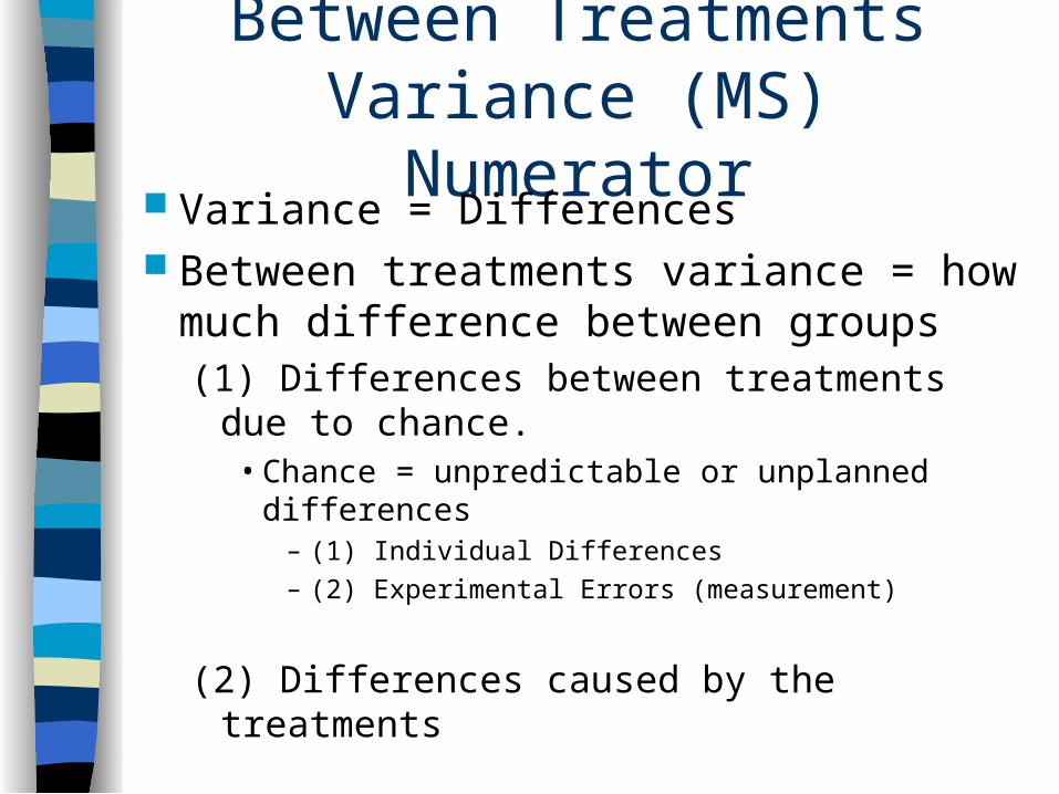
Between Treatments Variance (MS)Numerator

Variance = Differences Between treatments variance = how

much difference between groups(1) Differences between treatments due to

chance.• Chance = unpredictable or unplanned

differences– (1) Individual Differences– (2) Experimental Errors (measurement)

(2) Differences caused by the treatments

Within Treatments Variance (MS)Denominator

Within - treatments variance = inside each treatment condition each participant is treated the same. Researcher doesn’t do anything to cause individual differences.

– But there is still variability between individuals

• Chance

Total Variability

Between-treatments

Variance

Within-treatments

Variance

Measures difference due to:

1. Chance

2. Treatment Effects

Measures difference due to:

1. Chance

Putting it Together: F - Ratio Total Variability (F) = MS Between

MS Within

OR

F = treatment + chance

chance

(1) Treatment has no effect = the numerator and denominator are only measuring chance, so ratio hovers near 1.

(2) Treatment has an effect ratio should be substantially > 1.

IMPORTANT NOTE: Since the denominator measures uncontrolled and unexplained variance it is called the ERROR TERM.

Putting it Together

What will happen to our F-ratio as the difference btwn treatment increases?

What will happen to our F-ratio as the difference within treatments increases?

What does an F-ratio of 1 mean?

ANOVA: Terms and Notation Levels = # of individual treatment

conditions that make up a factor (notated by k…for independent samples k also specifies the number of samples).

n = # of scores in each level or treatment (k).

N = total number of scores in the entire study (note that this is not the population just the n from all samples).

T = X for each treatment condition (total)

G = T for the entire study (grand total)

Let’s look with our Example

A single factor design - IV = # children in a single birthing experience

Levels: k = 3 ( # conditions that make up our factor) n = 5 for each level (note this could be different across

levels). (# of scores in each level) N = 15 (total number of scores) T1 = 40; T2 = 30; T3 = 20 (X for each treatment condition). G = 90 (T for the entire study)

Single Child Twins Triplets8 4 47 6 4

10 7 76 4 29 9 3

ANOVA Formulas Final Calculation is the F-ratio:

F = variance between treatments

variance within treatment

where s2 = SS / df The entire process of ANOVA will take

9 calculations!– 3 SS values: SS total; SS btwn; SS w/in– 3 df values: df total; df btwn; df w/in– 2 variances: MS btwn & MS w/in– F-ratio

Analysis of SS Reminder: SS = X2 - ((X)2 / N) First we calculate the total and then each part; between

and within SStotal = X2 - (G2 / N) = 622 - (902 / 15) = 82

SSw/in = SSinside each treatment = 10 + 18 + 14 = 42

SSbtwn = (T2 / n) - (G2 / N)

= ((402 / 5) + (302 / 5) + (202 / 5) )- (902 / 15)

= 320 + 180 + 80 - 540 = 40 CHECK: SStotal = SSw/in + SSbtwn; 82 = 42 + 40

K = 3 X2 = 622

n = 5 each

N = 15

G = 90

Single Child Twin Triplet8 4 47 6 4

10 7 76 4 29 9 3

40 30 20

Review: Breaking down SS

SStotal

X2 - (G2 / N)

SSw/in

SSinside each treatment

SSbtwn

(T2 / n) - (G2 / N)

Note: So far, we’ve completed 3 of the 9 calculations!

Analysis of Degrees of Freedom Again, first we calculate the total and then each part;

between and within. Remember:

– Each df is associated with a specific SS value.– Normally the value of SS is obtained by counting the number

of items that were used to calculate SS and then subtract 1.

dftotal = N - 1 (this SS values measure the total variability) = 15 - 1 = 14

dfwithin = (n-1) = dfeach treatment = 4 + 4 + 4 = 12or N - k = 15 - 3 = 12

dfbetween = k - 1 (# T values or samples - 1) = 3 - 1 = 2 CHECK: dftotal = dfwithin + dfbetween; 14 = 12 + 2

K = 3 X2 = 622

n = 5 each

N = 15

G = 90

Single Child Twin Triplet8 4 47 6 4

10 7 76 4 29 9 3

40 30 20

Review: Breaking down dfdftotal

N - 1

dfw/in

N - k or dfeach treatment

dfbtwn

k - 1

Note: So far, we’ve completed 6 of the 9 calculations!

Analysis of MS and F - ratio In ANOVA it is convention to use the

term mean square or MS instead of variance or s2.

MS = variance = SS / df MSbetween = SSbetween / dfbetween

= 40 / 2 = 20

MSwithin = SSwithin / dfwithin

= 42 / 12 = 3.5

F = MSbetween / MSwithin

= 20 / 3.5 = 5.7

So we’re greater than 1 which is better than chance, but so far we don’t know about significance

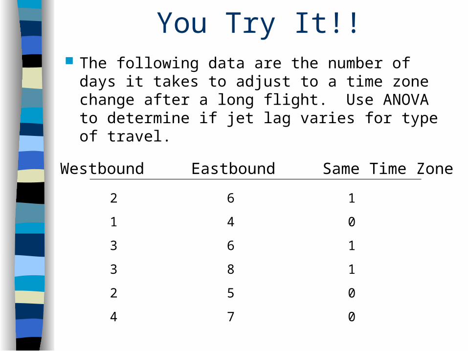
You Try It!! The following data are the number of days it

takes to adjust to a time zone change after a long flight. Use ANOVA to determine if jet lag varies for type of travel.

Westbound Eastbound Same Time Zone

2

1

3

3

2

4

6

4

6

8

5

7

1

0

1

1

0

0

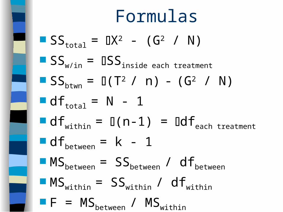
Formulas SStotal = X2 - (G2 / N)

SSw/in = SSinside each treatment

SSbtwn = (T2 / n) - (G2 / N)

dftotal = N - 1

dfwithin = (n-1) = dfeach treatment

dfbetween = k - 1

MSbetween = SSbetween / dfbetween

MSwithin = SSwithin / dfwithin

F = MSbetween / MSwithin

So, Now What? Hypothesis Testing!(1) State the hypotheses: Note. The hypotheses are

stated in terms of population parameters even though we use sample data to test them. Let’s use our example.

H0 = μ1 = μ2 = μ3 (no treatment effect)

H1 = At least one of the treatment means is different. In general H1 states that the treatment treatment

conditions are not all the same; so there is a real effect. Note: we do not give any specific alternative hypothesis.

This is because many different alternatives are possible and it would be tedious to list them all (& researcher typically have predictions).– e.g. H1 = μ1 = μ2 = μ3 or H1 = μ1 = μ3, but μ2 is different

Hypothesis Testing: Setting the critical region

(2) Set the critical region - But first we need to know something about

the distribution of F-ratios.– Because F -ratios are computed from 2 variances

(the numerator and denominator), F values will always be positive numbers.

• This comes from the fact that in order to calculate SS we have to square values, right?!

– When H0 is true the numerator and denominator are both measuring the same variance (chance or error). They should be roughly the same size, so F-ratio should equal 1.

• This means scores in our distribution (remember the distribution we test against is the null distribution) should pile up around 1.

Distribution of F-ratios The distribution is cut off at 0. The means pile up around 1 and then taper

off to the right (positively skewed). Like the t-distribution the exact F distribution

depends on df.– Large df provides a more accurate estimate of

population variance & F-ratios piled around 1.– Small df will result in a more spread out

distribution

Large df Small df

Hypothesis Testing: Setting the Critical Region

(2) Set the critical region. (In our example .05 2-tailed.)

We need to know the degrees of freedom for our F-ratio.– df between (in our example dfbetween = 2)– df within (in our example dfwithin = 12)

Use the F-distribution table (pg. 693)– df values for the numerator are printed across the top– df values for the denominator are printed in the column

on the left-hand side– Our example is said to have “degrees of freedom

equal to 2 and 12”. So, critical value is 3.88

NOTE: With ANOVA is it okay to set the critical region after we have calculated our df values in Step 3 (collect data and compute test stat).

Hypothesis Testing: Calculate the Test Statistic

(3) Collect the data and calculate the test statistic.

We already did this:– Remember there are 9 calculations

involved in computed an ANOVA• 3 for SS• 3 for df• 2 for MS• 1 for F-ratio

Hypothesis Testing: Make a Decision

(4) Make a decision.

The F-ratio we calculated was 5.7. This is greater than our critical value of 3.88, so we can reject the null hypothesis.

There is a significant treatment effect. But we don’t know which of our means are different. We can only say that at least one difference exists

Let’s Do One: Hypothesis Testing with ANOVA

A psychologist would like to examine the relative effectiveness of 3 therapy techniques for treating mild phobias. A sample of N = 18 individuals who display a moderate fear of spiders is obtained. The dependent variable is a measure of reported fear of spiders after therapy.

NOTE: While you can do ANOVA with unequal sample sizes, which is what this example is going to show ANOVA is most accurate when sample sizes are equal. Therefore, when possible researchers should try to equate across samples. However, ANOVA will still be a valid test, especially when sample sizes are large and the discrepancy between sample sizes is not huge.

Let’s Do One: Hypothesis Testing with ANOVA

Therapy A Therapy B Therapy C5

5

2

2

4

2

3

3

0

2

2

1

0

1

2

1

1

3T = 20

SS = 11.33

n = 6

T = 10

SS = 6

n = 5

T = 9

SS = 5.43

n = 7

G = 39

X2 = 121

N = 18

Formulas SStotal = X2 - (G2 / N)

SSw/in = SSinside each treatment

SSbtwn = (T2 / n) - (G2 / N)

dftotal = N - 1

dfwithin = (n-1) = dfeach treatment

dfbetween = k - 1

MSbetween = SSbetween / dfbetween

MSwithin = SSwithin / dfwithin

F = MSbetween / MSwithin

Effect Size in ANOVA Simplest and most direct measure is r2, the

percentage of variance accounted for by the treatment

r2 = SSbetween treatments

SSbetween treatments + SSwithin treatments (total)

r2 when computed for ANOVA is usually called 2

Compute the effect size for the previous example

In the Literature The means and standard deviations are

presented in Table 1. The analysis of variance (ANOVA) revealed a significant difference, F(2, 15) = 4.52, p < .05, 2 = .38

Therapy A Therapy B Therapy CM 3.33 2 1.29SD 1.51 1.22 0.95

Post Hoc Tests F is an omnibus test: it just says that the

means differ, but not which ones. We have to do additional tests to determine.

When are post hoc tests done? As the name implies after an ANOVA– But only after a rejection of the null hypothesis.– Only if there are 3 more more treatments; k 3. If

only 2 treatments we can just do a t-test. Post hoc tests are going to let us go back

through our data and compare individual treatments 2 at a time.– So in our original example we can compare: single

v. twin, single v. triplets, twins v. triplets.

Post Hoc Tests Why can’t we do multiple t-tests?

– Risk of Type I error accumulates!– If alpha = .05 then we have a 5% chance of a Type I

error or 1 out of 20 chance. • So, for every 20 tests we perform we should expect 1 out

of 20 to be a Type I error.• If we perform multiple t-tests we increase the likelihood of

Type I error (probability doesn’t simply sum, but does increase).

Experimentwise alpha level: the overall possibility of committing a Type I error over a series of separate hypotheses tests.– Usually the experimentwise alpha level is quite a bit

larger than the value of alpha used for any individual test.

Post hoc tests have been designed to control the experimentwise alpha level, so we control the number of Type I errors we are willing to make.

Tukey’s Honestly Significant Difference (HSD) Test

HSD - allows us to compute a single value that determines the minimum difference between any two treatments necessary for significance.

This difference is used to compare any 2 treatment conditions

Formula: HSD = q MSwithin / n

– Where q is found in table B.5 page 698.– Tukey assumes that n is the same size across samples

(can’t use with ANOVA that uses diff. sample sizes)– Alpha should be the same as the alpha you set in original F-

test.

Let’s Try HSD HSD = q MSwithin / n Let’s use our original example with births and

language: n = 5 k = 3 MSwithin = 3.5 dfwithin = df (error term) = 12 M1 = 8, M2 = 6, M3 = 4 TEST EACH

– Single v. Twins– Single v. Triplets– Twins v. Triplets

Single Child Twin Triplet8 4 47 6 4

10 7 76 4 29 9 3

40 30 20

You Try One HSD = q MSwithin / n

Use your flight data….Westbound Eastbound Same Time Zone

2

1

3

3

2

4

M = 2.5

6

4

6

8

5

7

M = 6

1

0

1

1

0

0

M = .5

n = 6

K = 3

Scheffe Test Most Conservative Method:

– Uses an F-ratio to test any 2 treatments• The numerator for MS between treatment is

recalculated comparing only the 2 treatments you want to look at – denominator stays the same

• The denominator for the F-ratio stays the same as overall ANOVA

– Although you are only comparing 2 treatment it still using the value of k to calculate the between treatments df (as k increases our critical value increases; see the table)

– Critical value for the F-ratio is going to be the same as the overall F-ratio critical.

Calculating the Sheffe Rather than calculate for all possible combinations

better to start with the largest difference and then test progressively smaller difference until we find one that is not significant

Single v. triplets SSbtwn = (T2 / n) - (G2 / N) = 402 / 5 + 202 / 5 - 602 / 10

= 40 MSbetween = SSbetween / dfbetween = 40 / 2 = 20

F = MSbetween / MSwithin = 20 / 3.5 = 5.71Single Child Twin Triplet

8 4 47 6 4

10 7 76 4 29 9 3

40 30 20

k = 3 X2 = 622

n = 5 each N = 15

G = 90

* Critical was 3.88. Now do the next one.

Assumptions of Independent Measures ANOVA

The observations within each sample must be independent.

The populations from which the samples are selected must be normal.

The populations from which the samples are selected must have equal variances (homogeneity of variance)

F - Max Revisited F - max is a test of homogeneity of variance (pg.

329).– Compute sample variance for each sample

• S2 = SS / df

– Select the largest and smallest of the sample variances and compute

• F - max = s2 (largest) / s2 (smallest)

– F - max assumes that each sample is the same size– Locate critical value in table B.3

– K = # of separate samples– Df = n - 1 (because each sample should be the same size)– Look at appropriate alpha level

– A large F-max value indicates a large diff. between s2 whereas a small F-max indicates a small diff. between s2.

• F-max value needs to be SMALLER than critical value to assume that we have homogeneity of variance.

Do F-Max with our Flight Data

Westbound Eastbound Same Time Zone

2

1

3

3

2

4

M = 2.5

SS = 5.5

6

4

6

8

5

7

M = 6

SS = 17

1

0

1

1

0

0

M = .5

SS = 1.5

n = 6 in each sample

K = 3

Homework

You will be responsible on the exam for reading pg. 430-431 relationship between ANOVA and t tests (pg 429-430).

Chapter 13– 1, 3, 4, 5, 6, 8, 9, 12, 17, 18, 19