Lecture 3: Micro-econ. ~ last topic (Profits) & Basics of

Macroeconomics - I Dr. Rajeev DhawanDr. Rajeev Dhawan

DirectorDirector Given to theGiven to the

EMBA 8400 ClassEMBA 8400 ClassApril 2, 2010April 2, 2010

Chapter 13

Costs & Profits

Cost of Production

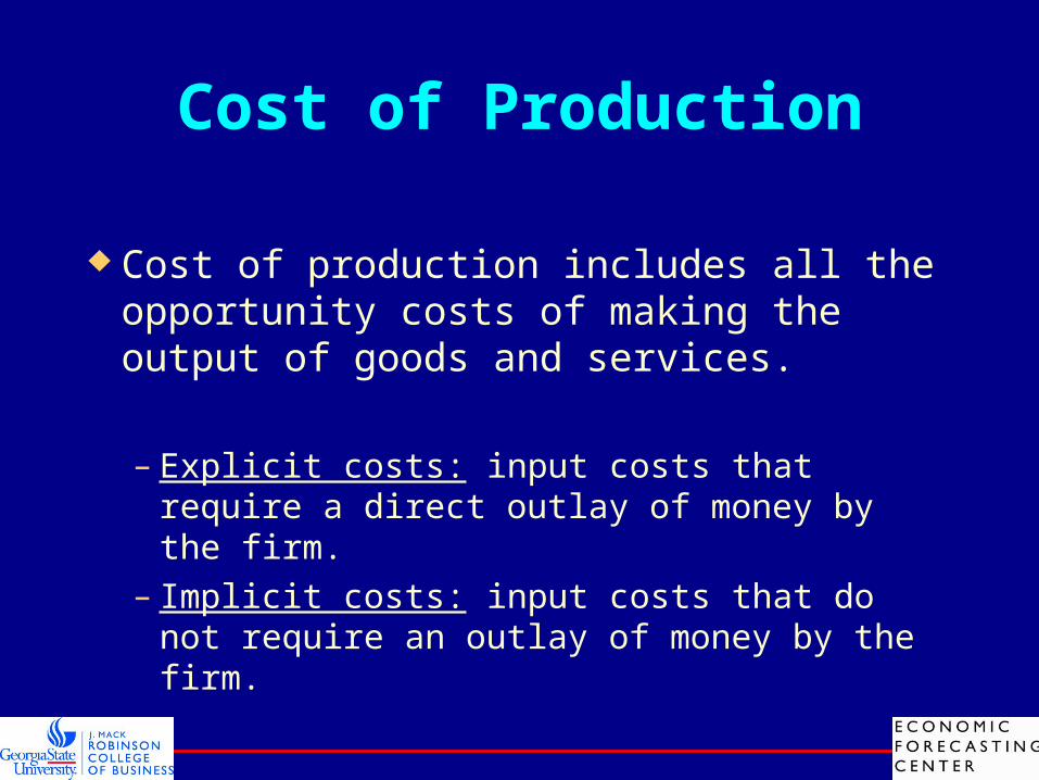
Cost of production includes all the opportunity costs of making the output of goods and services.

– Explicit costs: input costs that require a direct outlay of money by the firm.

– Implicit costs: input costs that do not require an outlay of money by the firm.

Profits

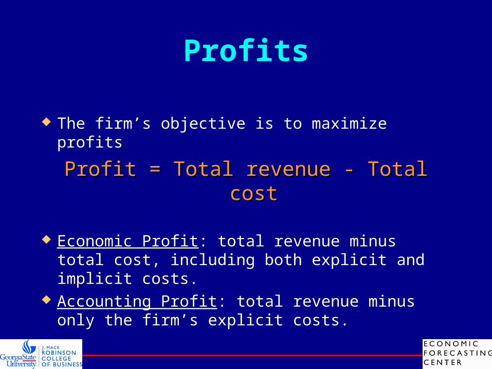
The firm’s objective is to maximize profits

Profit = Total revenue - Total costProfit = Total revenue - Total cost

Economic Profit: total revenue minus total cost, including both explicit and implicit costs.

Accounting Profit: total revenue minus only the firm’s explicit costs.

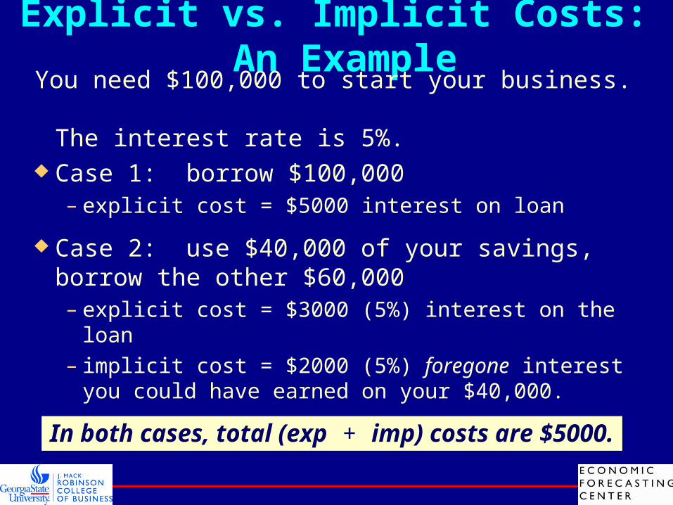
Explicit vs. Implicit Costs: An ExampleYou need $100,000 to start your business.

The interest rate is 5%. Case 1: borrow $100,000

– explicit cost = $5000 interest on loan

Case 2: use $40,000 of your savings, borrow the other $60,000– explicit cost = $3000 (5%) interest on the loan– implicit cost = $2000 (5%) foregone interest you

could have earned on your $40,000.In both cases, total (exp + imp) costs are $5000.

Profits

Copyright © 2004 South-Western

Revenue

Totalopportunitycosts

How an EconomistViews a Firm

How an AccountantViews a Firm

Revenue

Economicprofit

Implicitcosts

Explicitcosts

Explicitcosts

Accountingprofit

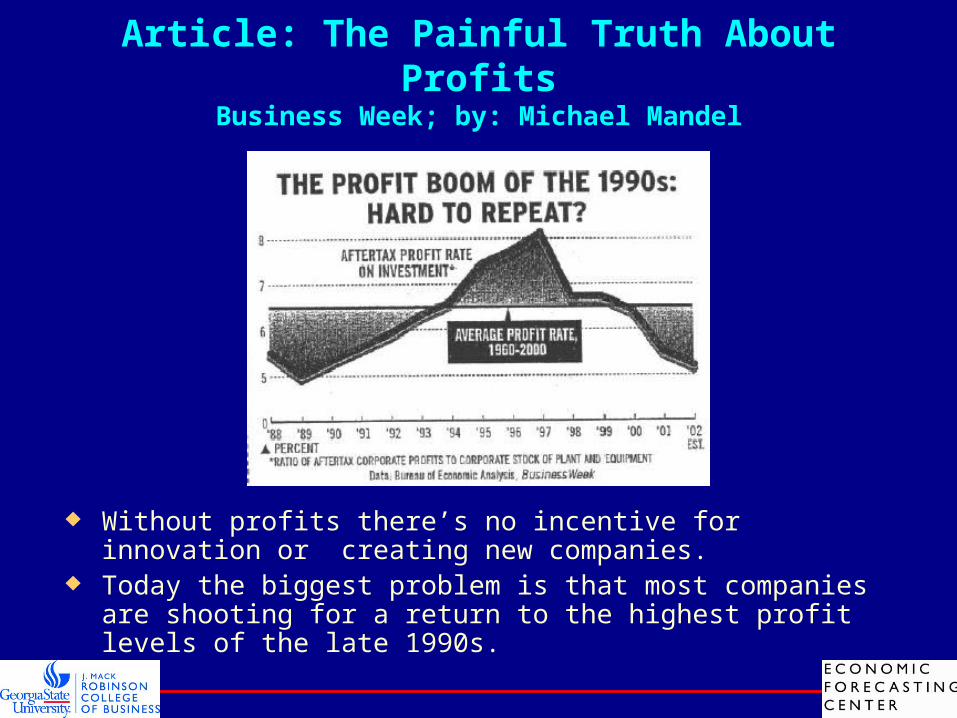
Article: The Painful Truth About ProfitsBusiness Week; by: Michael Mandel

Without profits there’s no incentive for innovation or creating new companies.

Today the biggest problem is that most companies are shooting for a return to the highest profit levels of the late 1990s.

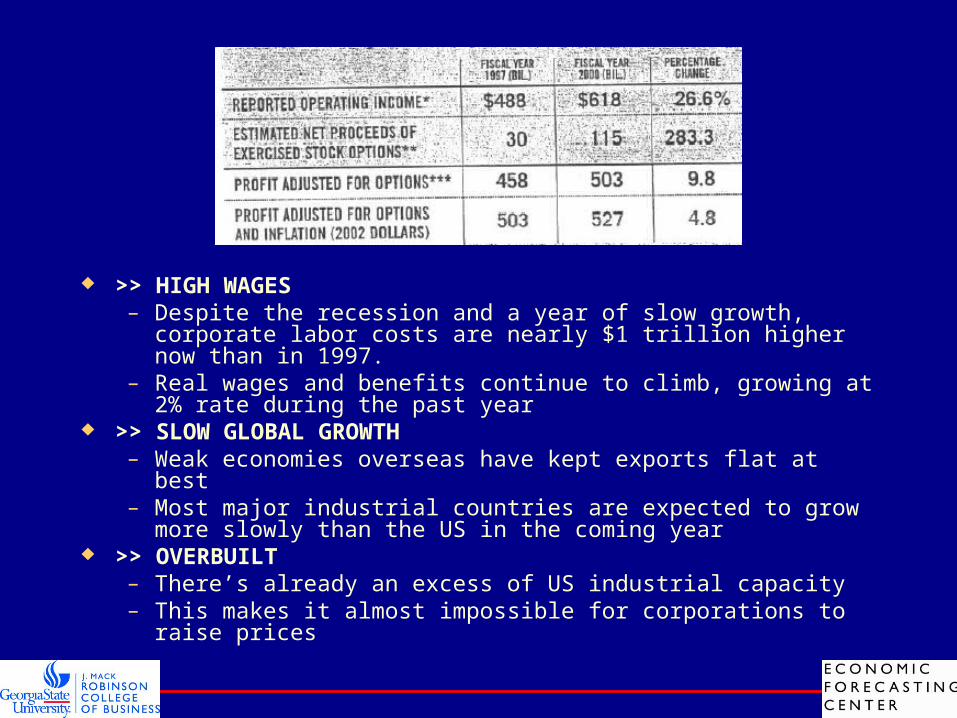
>> HIGH WAGES– Despite the recession and a year of slow growth, corporate labor

costs are nearly $1 trillion higher now than in 1997.– Real wages and benefits continue to climb, growing at 2% rate

during the past year >> SLOW GLOBAL GROWTH

– Weak economies overseas have kept exports flat at best– Most major industrial countries are expected to grow more slowly

than the US in the coming year >> OVERBUILT

– There’s already an excess of US industrial capacity– This makes it almost impossible for corporations to raise prices

Article: Economic Profit vs. Accounting ProfitWSJ; by Robert Bartley

Profit is any income to a proprietor—Marxist Labor View—which is fallacious

The economist is interested in the dynamic forces of production while: The accountant is interested in proprietorship….cost as a deduction from the owner’s income

Economic profit is the unimputable income i.e. “the residium of product remaining after payment is made at rates established in competition with all comers for all services of men or things for which competition exists”

The highest uses depend on economic profit-rate of return on assets-not on accounting profits.

The issue of interest on equity has tended to constitute an issue between accountants and economic theorists

EPS measures the corporate profit and is called the accounting profit Peter Drucker: EPS represents taxable earnings i.e. after all deductions, is

purely arbitrary concept and has nothing to do with business performance NET-NET: Takes skill to convert EPS into meaningful economic profit

concept.

Marginal Product Marginal Product: for any input, it is the increase in output

that arises from an additional unit of that input. Diminishing Marginal Product: the marginal product of an

input declines as the quantity of the input increases.

0

0.5

1

1.5

2

2.5

3

3.5

0 2 4 6 8 10

Y = Y = √I√II Y MP0 0

1.01 1

0.42 1.4

0.33 1.7

0.34 2

0.25 2.2

Diminishing Marginal ProductQuantity of

Output(cookiesper hour)

150

140

130

120

110

100

90

80

70

60

50

40

30

20

10

Number of Workers Hired0 1 2 3 4 5

Production function

I Y MP0 0

501 50

402 90

303 120

204 140

105 150

Fixed & Variable Costs

Fixed costs: those costs that do not vary with the quantity of output produced.

Variable costs: those costs that do vary with the quantity of output produced.

TCTC = = TFCTFC + + TVCTVC Total Costs

– Total Fixed Costs (TFC)– Total Variable Costs (TVC)– Total Costs (TC) – TC = TFC + TVC

Total Cost Curve Shows the relationship between the quantity

a firm can produce and its costs.

Total Cost CurveTotalCost

$80

70

60

50

40

30

20

10

Quantity of Output(cookies per hour)

0 10 20 30 15013011090705040 1401201008060

Total-costcurve

Marginal Cost

Marginal Cost (MC): measures the increase in total cost that arises from an extra unit of production.

M CTCQ

( ch an g e in to ta l co st)

(ch an g e in q u an tity )

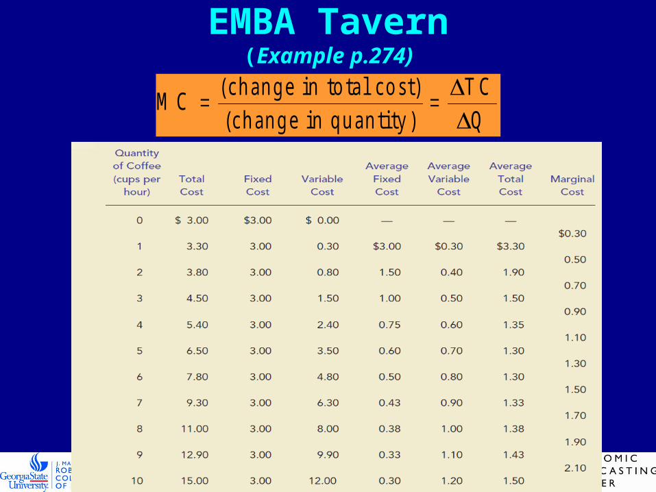
EMBA Tavern(Example p.274)

M CTCQ

( ch an g e in to ta l co st)

(ch an g e in q u an tity )

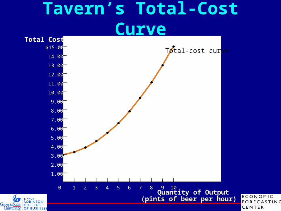
Tavern’s Total-Cost CurveTotal Cost

$15.00

14.00

13.00

12.00

11.00

10.00

9.00

8.00

7.00

6.00

5.00

4.00

3.00

2.00

1.00

Quantity of Output(pints of beer per hour)

0 1 432 765 98 10

Total-cost curve

Average Costs

Average costs can be determined by dividing the firm’s costs by the quantity of output it produces.

The average cost is the cost of each typical unit of product. – ATC – AFC – AVC

Tavern’s Various Cost CurvesCosts

$3.50

3.25

3.00

2.75

2.50

2.25

2.00

1.75

1.50

1.25

1.00

0.75

0.50

0.25

Quantity of Output(pints of beer per hour)

0 1 432 765 98 10

MC

ATC

AVC

AFC

Returns/Economies of Scale

Increasing Returns to Scale/Economies of scale (IRS): long-run average total cost falls as the quantity of output increases.

Decreasing Returns to Scale/Diseconomies of scale (DRS): long-run average total cost rises as the quantity of output increases.

Constant returns to scale (CRS): long-run average total cost stays the same as the quantity of output increases

Economies of Scale (P 279)

Quantity ofCars per Day

0

AverageTotalCost

1,200

$12,000

1,000

10,000

ATC in long run

Constantreturns to

scale

Increasing

scalereturns to

Decreasing

scalereturns to

Chapter 14

Competitive Firms

Total Revenue

Total Revenue: for a firm, is the selling price times the quantity sold.

TR = (P TR = (P Q) Q)

Total revenue is proportional to the amount of output.

Average Revenue Average Revenue: how much revenue a

firm receives for the typical unit sold.

A v erag e R ev en u e =T o ta l rev en u e

Q u an tity

P rice Q u an tity

Q u an tity

P rice

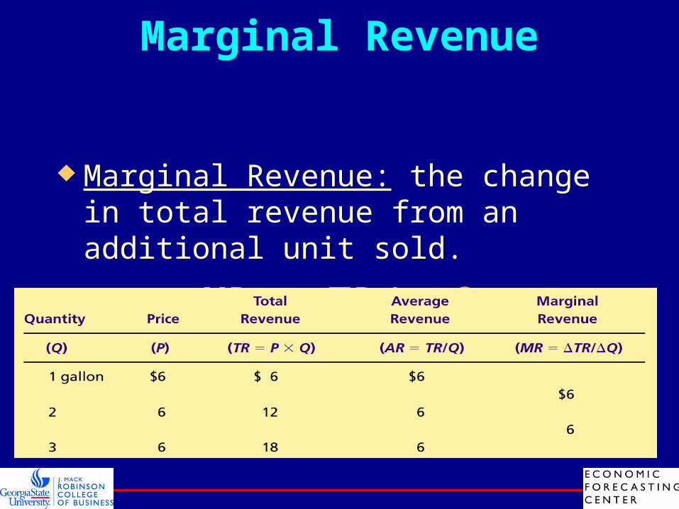
Marginal Revenue

Marginal Revenue: the change in total revenue from an additional unit sold.

MR =MR =TR/ TR/ QQ For competitive firms, marginal revenue

equals the price of the good.

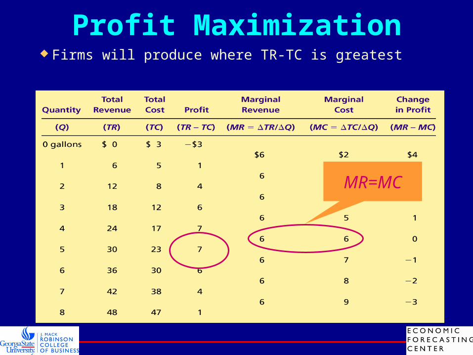
Profit Maximization Firms will produce where TR-TC is greatest

MR=MC

Profit Maximization

Quantity0

Costsand

Revenue

MC

ATC

AVC

MC1

Q1

MC2

Q2

The firm maximizesprofit by producing the quantity at whichmarginal cost equalsmarginal revenue.

QMAX

P = MR = MC P = AR = MR

Measuring Profits Graphically

Quantity0

Price

P = AR = MR

ATCMC

P

ATC

Q(profit-maximizing quantity)

Firm withProfits

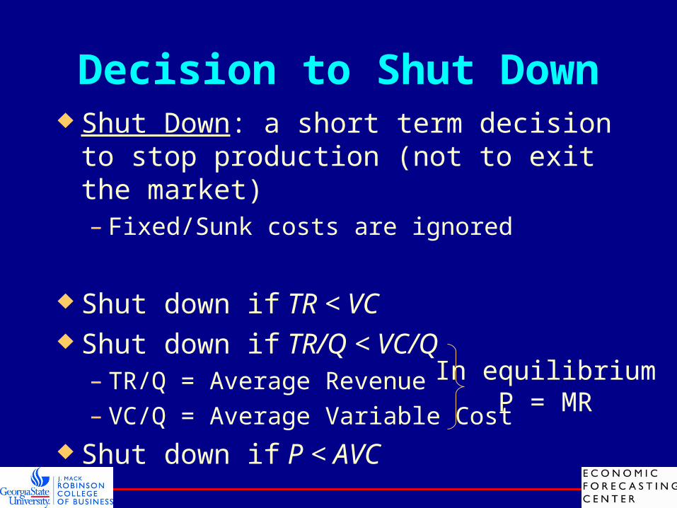
Decision to Shut Down Shut Down: a short term decision to stop

production (not to exit the market)– Fixed/Sunk costs are ignored

Shut down if TR < VC Shut down if TR/Q < VC/Q

– TR/Q = Average Revenue– VC/Q = Average Variable Cost

Shut down if P < AVC

In equilibriumP = MR

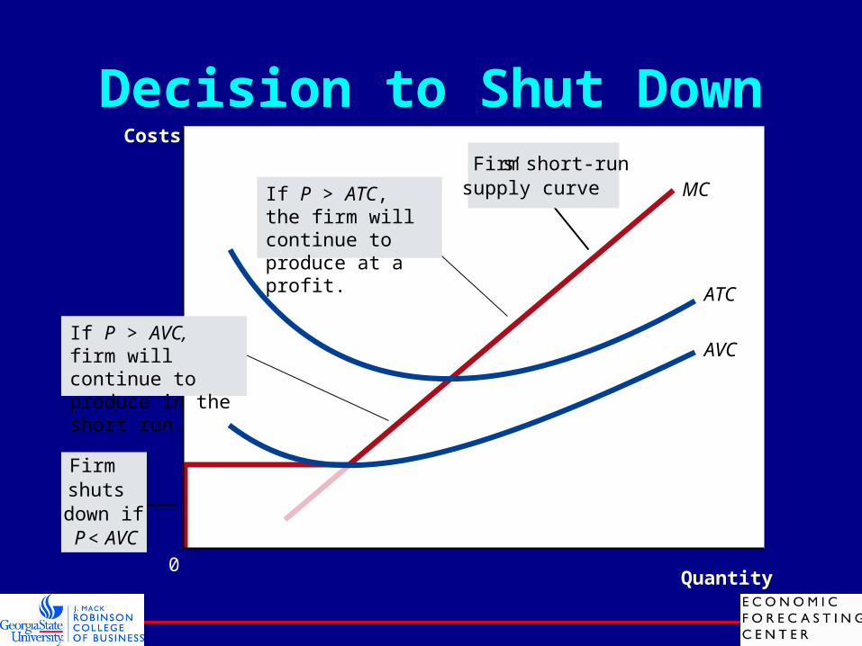
Decision to Shut Down

MC

Quantity

ATC

AVC

0

Costs

Firmshutsdown ifP< AVC

Firm’s short-runsupply curve

If P > AVC, firm will continue to produce in the short run.

If P > ATC, the firm will continue to produce at a profit.

Decision to Exit

Exit: a long run decision to leave the market The firm exits if the revenue it would get

from producing is less than its total cost.

Exit if TR < TC Exit if TR/Q < TC/Q Exit if P < ATC

Decision to Exit

MC = long-run S

Firmexits ifP < ATC

Quantity

ATC

0

CostsFirm’s long-runsupply curve

Firmenters ifP > ATC

Measuring Profits Graphically

Quantity0

Price

ATCMC

(loss-minimizing quantity)

P = AR = MRP

ATC

Q

Loss

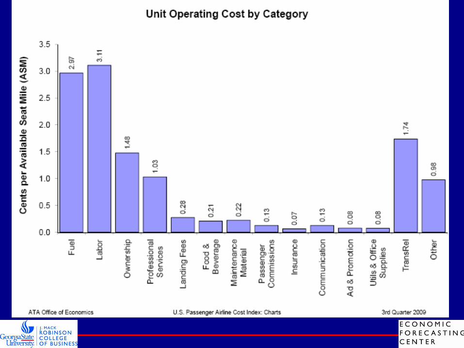
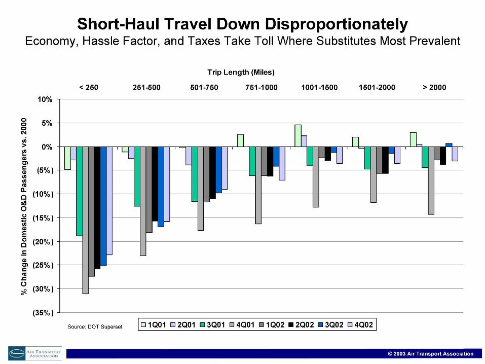
Cost & Profits

Airline Industry

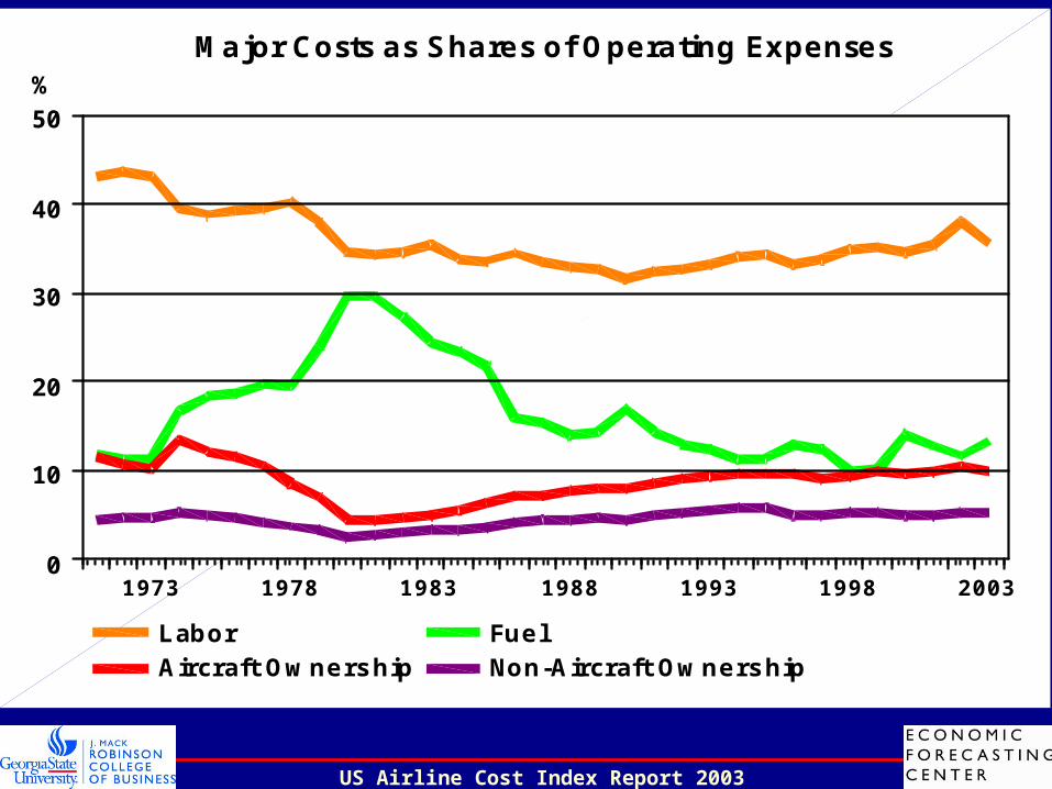
2003199819931988198319781973

50

40

30

20

10

0

% Major Costs as Shares of Operating Expenses

Labor FuelAircraft Ownership Non-Aircraft Ownership

US Airline Cost Index Report 2003

US Airline Cost Index Report 2004

ATA 2004 Economic Report

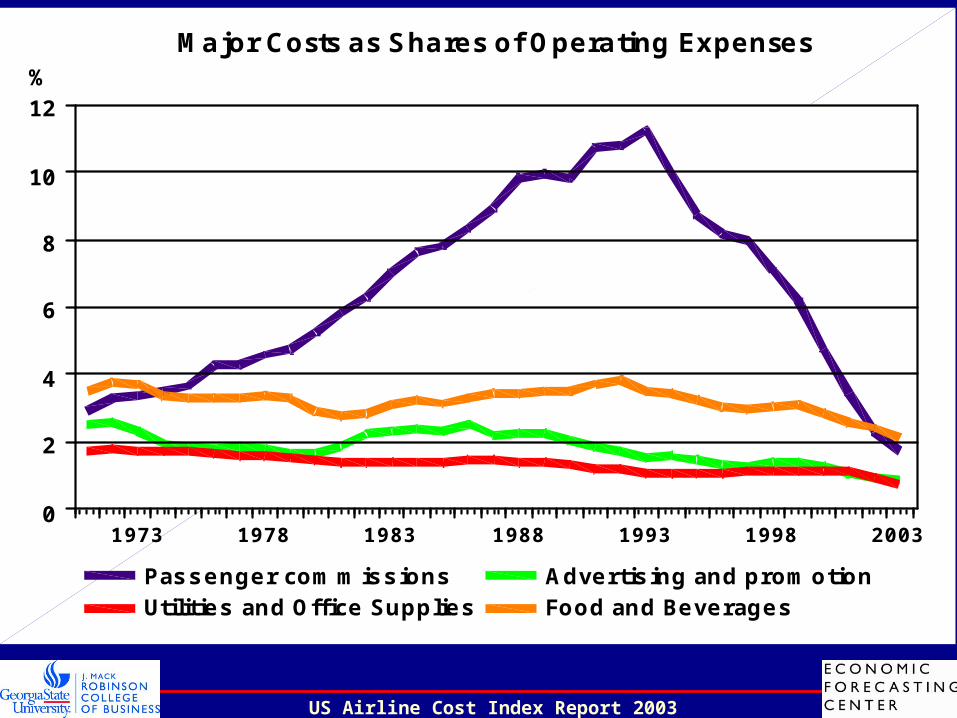
2003199819931988198319781973

12

10

8

6

4

2

0

% Major Costs as Shares of Operating Expenses

Passenger commissions Advertising and promotionUtilities and Office Supplies Food and Beverages

US Airline Cost Index Report 2003

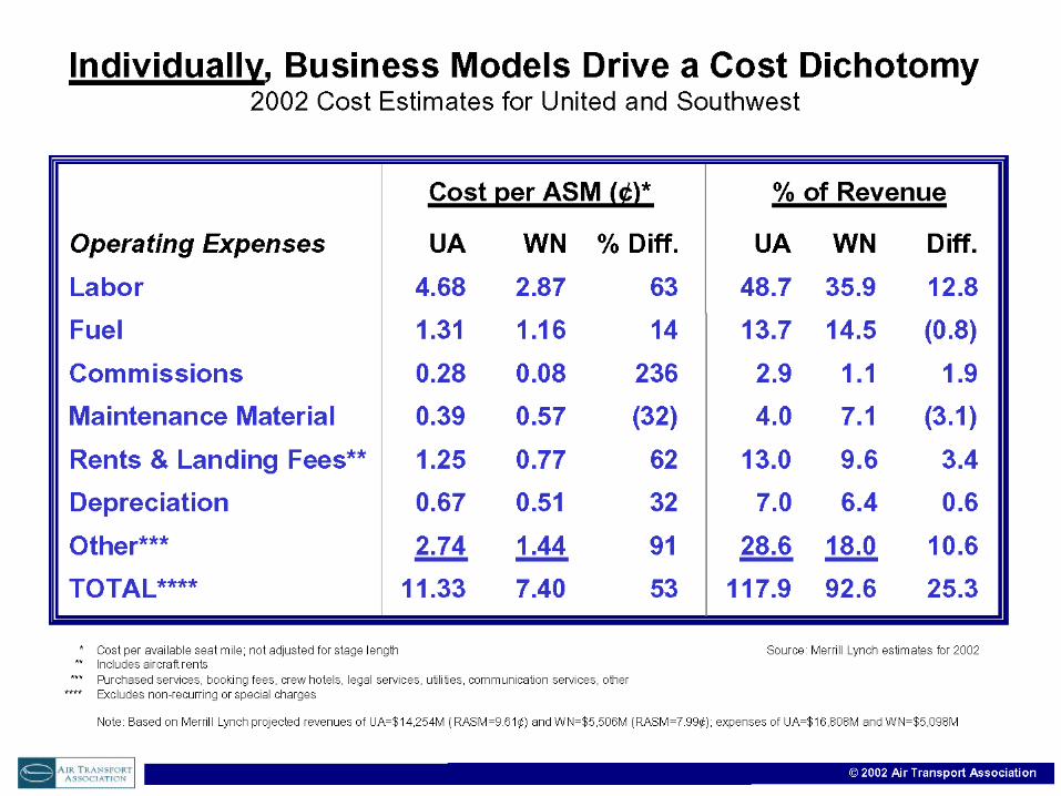
Article: One Airline’s MagicTime Magazine by: Sally Donnelly

How does Southwest (SW) soar above its money losing rivals?

ProductivityIts employees work harder and are smarter, in return, they get job security and a share of profits– Pilots fly as many as 83 hours a month, compared with about 53

hours in a busy month at United Airlines– Flight attendants work almost twice as many hours as their

counterparts at other airlines– Mechanics change airplane tires faster (like a NASCAR pit) and thus

get higher wages than their counterparts at other airlines

Flexibility– SW pilots also pitch in to help ground crews move luggage

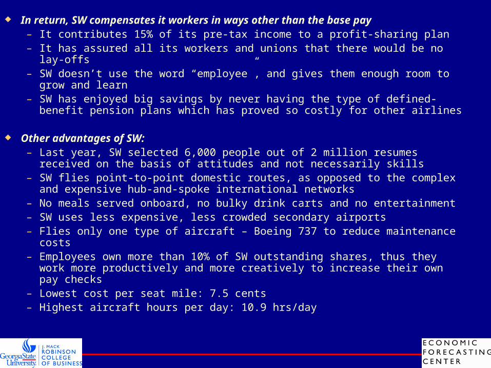
In return, SW compensates it workers in ways other than the base pay– It contributes 15% of its pre-tax income to a profit-sharing plan– It has assured all its workers and unions that there would be no lay-offs– SW doesn’t use the word “employee”, and gives them enough room to grow

and learn– SW has enjoyed big savings by never having the type of defined-benefit

pension plans which has proved so costly for other airlines

Other advantages of SW:– Last year, SW selected 6,000 people out of 2 million resumes received on

the basis of attitudes and not necessarily skills– SW flies point-to-point domestic routes, as opposed to the complex and

expensive hub-and-spoke international networks– No meals served onboard, no bulky drink carts and no entertainment– SW uses less expensive, less crowded secondary airports– Flies only one type of aircraft – Boeing 737 to reduce maintenance costs– Employees own more than 10% of SW outstanding shares, thus they work

more productively and more creatively to increase their own pay checks– Lowest cost per seat mile: 7.5 cents– Highest aircraft hours per day: 10.9 hrs/day

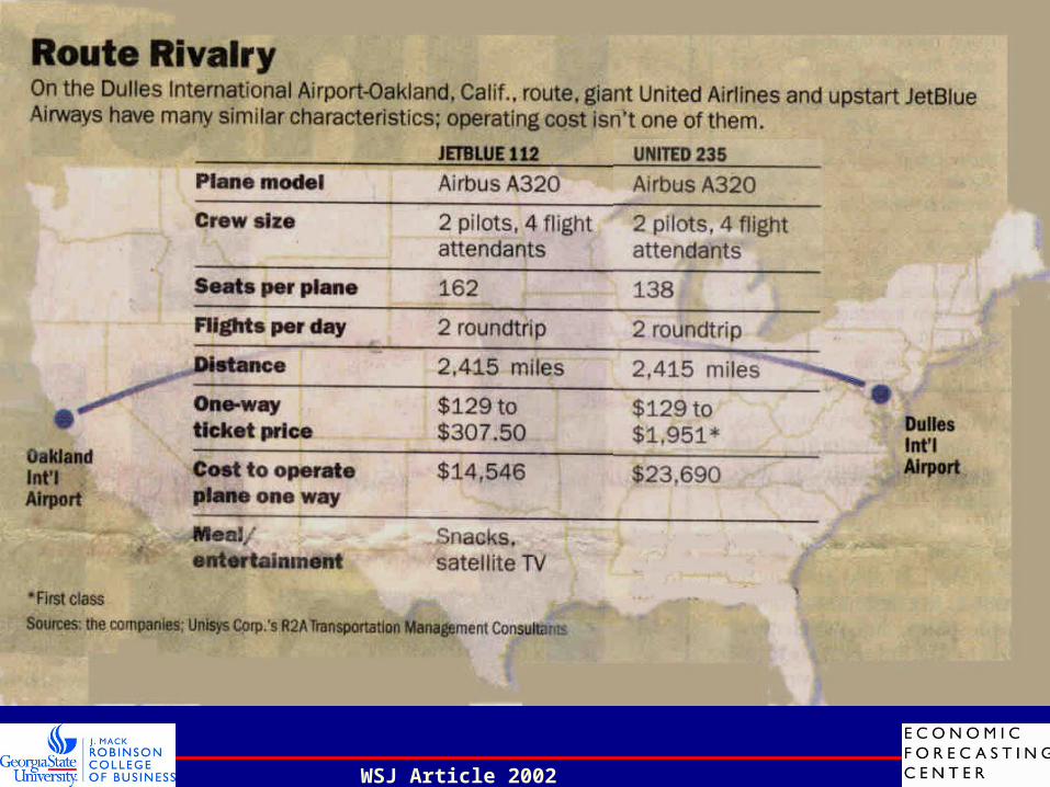
WSJ Article 2002

So What is the Solution?

Do the legacy airlines have any comparative advantage that they can use in competing with their low cost rivals for domestic travelers?

– The honest answer is NO.The time has come for some of the airlines to either merge or liquidate so that excess capacity in the market can be reduced to profitability manage the new demand frontier. (permanent downward shift in demand curve esp. domestic flying)But will the mergers or liquidations save the big boys? Maybe…The only way out is a radical shift in thinking by the big airlines: outsource to low-cost airlines and allow them to bring passengers to your legacy hubs! Then fly these travelers to international destinations on your planes at premium prices where there is no competition from South-West and upstart airlines.

Basics of Macroeconomics

Chapter 23

Macro Framework

Households: Consume & Work Firms: Production & Investment Government: Money Supply, Taxes,

Expenditures Foreign Sector: Exports, Imports &

Exchange Rate

The Economy’s Income & Expenditure

For an economy as a whole, income must equal expenditure because:– Every transaction has a buyer and a seller.– Every dollar of spending by some buyer is a dollar of

income for some seller. Gross domestic product (GDP)Gross domestic product (GDP) is a measure of the

income and expenditures of an economy. It is the total market value of all final goods and

services produced within a country in a given period of time.

Simple GDP Example

This simple economy has 2 people: Baker and Miller.Baker buys flour for $350. He also uses a worker and pays

$200 in wages. He also pays a rent of $25. He makes a profit as $25 on the bread he sells for $600.

The miller pays his worker $300, a rent of $25, and his profit is $25 on a sale of $350.

The GDP of this economy is $600!Why? 2 sides of a coin, Income=ExpendituresExpenditures=Value of final Goods sold=600Income=wages+Rent+profits=300+200+25+25+25+25=600

Definition of GDP

“GDP is the Market Value . . .”– Output is valued at market prices.

“. . . Of All Final . . .”– It records only the value of final goods, not

intermediate goods (the value is counted only once).

“. . . Goods and Services . . . “– It includes both tangible goods (food, clothing, cars)

and intangible services (haircuts, housecleaning, doctor visits).

Definition of GDP

“. . . Produced . . .”– It includes goods and services currently produced, not

transactions involving goods produced in the past.

“ . . . Within a Country . . .”– It measures the value of production within the

geographic confines of a country.

“. . . In a Given Period of Time.”– It measures the value of production that takes place

within a specific interval of time, usually a year or a quarter (three months).

Definition of GDP

What Is Not Counted in GDP?– GDP excludes most items that are produced and

consumed at home and that never enter the marketplace.

– It excludes items produced and sold illicitly, such as illegal drugs.

GDP and Economic Well-Being GDP per person tells us the income and

expenditure of the average person in the economy. Higher GDP per person indicates a higher standard of living.

However…GDP is not a perfect measure of the happiness or quality of life.

Some things that contribute to well-being are not included in GDP.– The value of leisure.– The value of a clean environment.– The value of almost all activity that takes place outside

of markets, such as the value of the time parents spend with their children and the value of volunteer work.

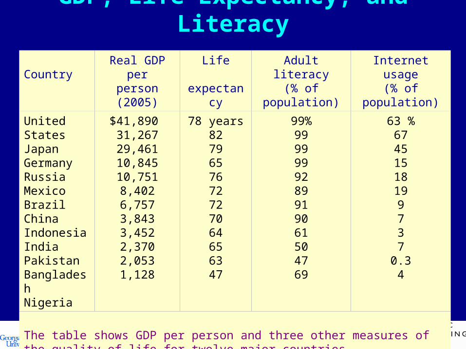
GDP, Life Expectancy, and Literacy

Country Real GDP perperson (2005)

Life expectancy

Adult literacy(% of population)

Internet usage(% of population)

United StatesJapan GermanyRussia Mexico Brazil China Indonesia India Pakistan Bangladesh Nigeria

$41,890 31,26729,46110,84510,7518,4026,7573,8433,4522,3702,0531,128

78 years 8279657672727064656347

99%9999999289919061504769

63 %67451518199737

0.34

The table shows GDP per person and three other measures of the quality of life for twelve major countries.

NIPA Definition of GDP

Y=C+I+G+NXY=C+I+G+NXY = GDPC = Consumption I = InvestmentG = Government PurchasesNX = Net Exports = Exports-Imports

NIPA Definition of GDP Consumption (C):Consumption (C):

– The spending by households on goods and services, with the exception of purchases of new housing.

Investment (I):Investment (I):– The spending on capital equipment, inventories, and

structures, including new housing. Government PurchasesGovernment Purchases (G) (G)::

– The spending on goods and services by local, state, and federal governments.

– Does not include transfer payments because they are not made in exchange for currently produced goods or services.

Net Exports (NX):Net Exports (NX):– Exports minus imports.

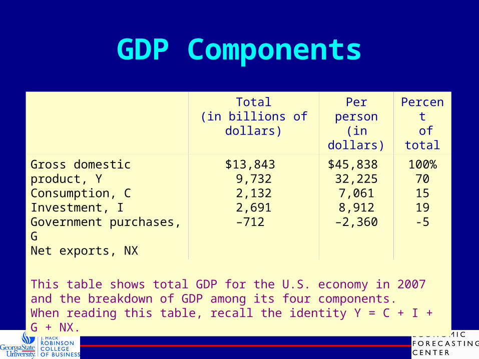
GDP Components

Total(in billions of dollars)

Per person(in dollars)

Percent of total

Gross domestic product, YConsumption, C Investment, I Government purchases, G Net exports, NX

$13,843 9,7322,1322,691–712

$45,838 32,2257,0618,912

–2,360

100%701519-5

This table shows total GDP for the U.S. economy in 2007 and the breakdown of GDP among its four components. When reading this table, recall the identity Y = C + I + G + NX.

Real vs. Nominal GDP

Nominal GDP values the production of goods and services at current prices.

Real GDP values the production of goods and services at constant prices. R eal G D P

N o m in a l G D P

G D P d efla to r2 0 X X2 0 X X

2 0 X X

1 0 0

•GDP Deflator deflates for Inflation!•Inflation is rate of change of prices.

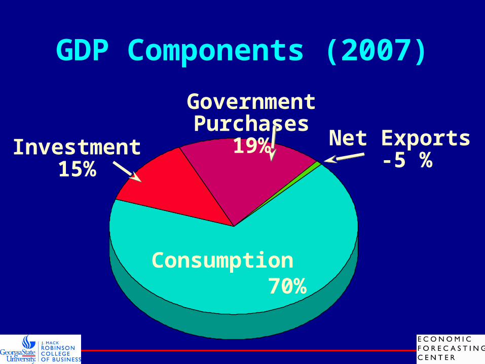
GDP Components (2007)

Consumption 70%

Government Purchases

19% Net Exports -5 %

Investment15%

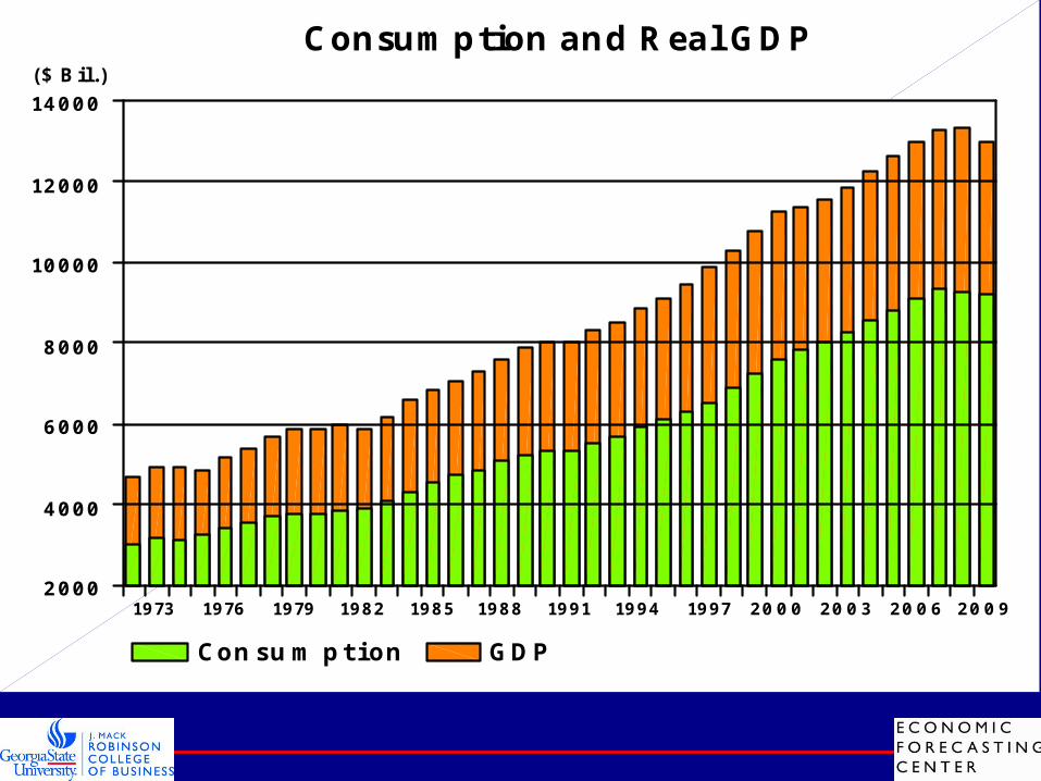
2009200620032000199719941991198819851982197919761973

14000

12000

10000

8000

6000

4000

2000

($ Bil.)Consumption and Real GDP

Consumption GDP

2009200520011997199319891985198119771973196919651961

72

70

68

66

64

62

60

(%)Consumption as a % of GDP

2009200520011997199319891985198119771973196919651961

20

18

16

14

12

10

(%)Investment as a % of GDP

2009200520011997199319891985198119771973196919651961

14

12

10

8

6

4

(%)Exports as a % of GDP

2009200520011997199319891985198119771973196919651961

18

16

14

12

10

8

6

4

2

(%)Imports as a % of GDP

2009200520011997199319891985198119771973196919651961

2

0

-2

-4

-6

-8

(%)Net Exports as a % of GDP

2009200520011997199319891985198119771973196919651961

24

23

22

21

20

19

18

17

(%)Government Spending as a % of GDP

2009200520011997199319891985198119771973196919651961

3

0

-3

-6

-9

-12

(%)Federal Deficit as a % of GDP