Lecture 5: Macroeconomic Model

Given to theGiven to theEMBA 8400 ClassEMBA 8400 Class

South Class Room #600South Class Room #600February 2, 2007February 2, 2007

Dr. Rajeev DhawanDr. Rajeev DhawanDirectorDirector

Important Macro Lessons To Be Learnt Today

GDP cannot grow beyond its potential in the long run

Loose Monetary Policy can create only a short-run stimulus in GDP. In long-run it only creates inflation! Net-Net money growth determines inflation

Government spending can create only a short-run stimulus in GDP. In the long-run it leads to a rise in the real interest rate with no gain in GDP but higher deficits

Balanced budget spending just redistributes the share of GDP attributed to consumption & government spending

world interest

rateworld GDP

IMPORTS

price level lag 1

worldprice

money

government

tax rate

capital stock lag 1

EXCHANGE RATE

INTEREST RATE

INVESTMENT

TAX REVENUES

investmentlag 1

EXPORTS

NETEXPORTS

REAL GDP

CONSUMPTION

DISPOSABLE INCOME

CAPITAL STOCK

inflationlag 1

PRICE LEVEL

INFLATION

EXPECTED INFLATION

UNEMPLOYMENT

POTENTIAL GDP

labor force

~~Typical Macro-ModelTypical Macro-Model~~

Macroeconomic Model

The Macroeconomic Model simulates the working of the US Economy using explicit equations to model consumption, investment, exports, imports, exchange rate, price level and inflation rate.

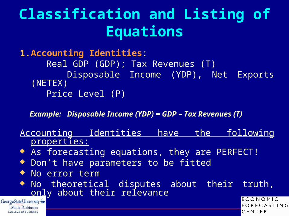
Classification and Listing of Equations

1. Accounting Identities: Real GDP (GDP); Tax Revenues (T) Disposable Income (YDP), Net Exports (NETEX) Price Level (P)

Example: Disposable Income (YDP) = GDP – Tax Revenues (T)

Accounting Identities have the following properties: As forecasting equations, they are PERFECT! Don’t have parameters to be fitted No error term No theoretical disputes about their truth, only about their

relevance

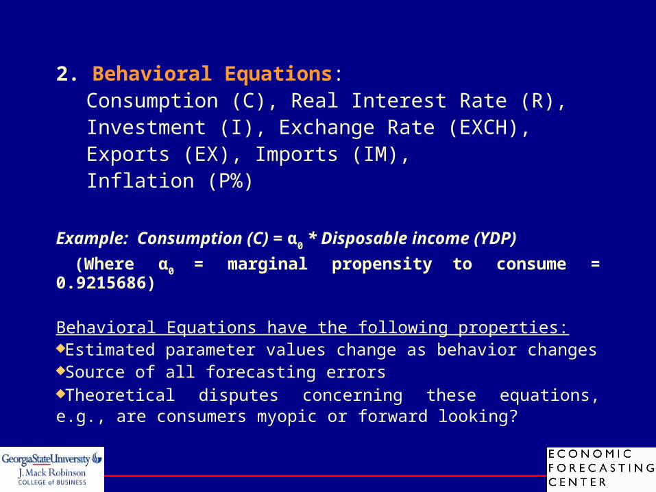
2. Behavioral Equations: Consumption (C), Real Interest Rate (R), Investment (I), Exchange Rate (EXCH), Exports (EX), Imports (IM), Inflation (P%)

Example: Consumption (C) = α0 * Disposable income (YDP)

(Where α0 = marginal propensity to consume = 0.9215686)

Behavioral Equations have the following properties:Estimated parameter values change as behavior changesSource of all forecasting errorsTheoretical disputes concerning these equations, e.g., are consumers myopic or forward looking?

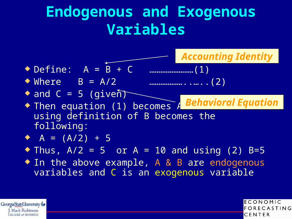
Endogenous and Exogenous Variables

Define: A = B + C ……………………(1) Where B = A/2 ………………..…..(2) and C = 5 (given) Then equation (1) becomes A = B +5 which

using definition of B becomes the following: A = (A/2) + 5 Thus, A/2 = 5 or A = 10 and using (2) B=5 In the above example, A & B are endogenous

variables and C is an exogenous variable

Accounting Identity

Behavioral Equation

Macroeconomic Model

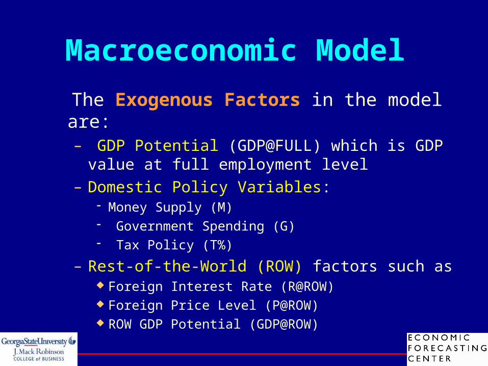
The Exogenous Factors in the model are:– GDP Potential (GDP@FULL) which is GDP value

at full employment level– Domestic Policy Variables:

Money Supply (M) Government Spending (G) Tax Policy (T%)

– Rest-of-the-World (ROW) factors such as Foreign Interest Rate (R@ROW) Foreign Price Level (P@ROW) ROW GDP Potential (GDP@ROW)

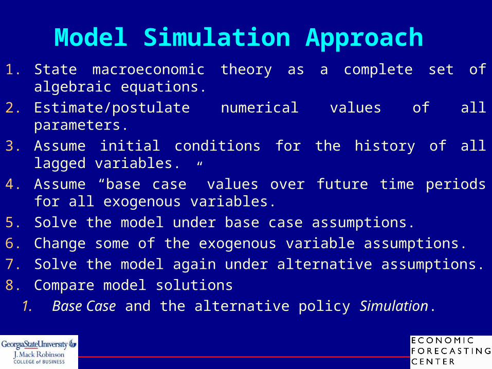
Model Simulation Approach 1. State macroeconomic theory as a complete set of algebraic

equations.

2. Estimate/postulate numerical values of all parameters.

3. Assume initial conditions for the history of all lagged variables.

4. Assume “base case” values over future time periods for all exogenous variables.

5. Solve the model under base case assumptions.

6. Change some of the exogenous variable assumptions.

7. Solve the model again under alternative assumptions.

8. Compare model solutions

1. Base Case and the alternative policy Simulation.

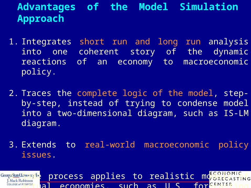
1. Integrates short run and long run analysis into one coherent story of the dynamic reactions of an economy to macroeconomic policy.

2. Traces the complete logic of the model, step-by-step, instead of trying to condense model into a two-dimensional diagram, such as IS-LM diagram.

3. Extends to real-world macroeconomic policy issues.

4. Same process applies to realistic models of actual economies, such as U.S. forecasting models, oil shocks, or world slowdown.

Advantages of the Model Simulation Approach

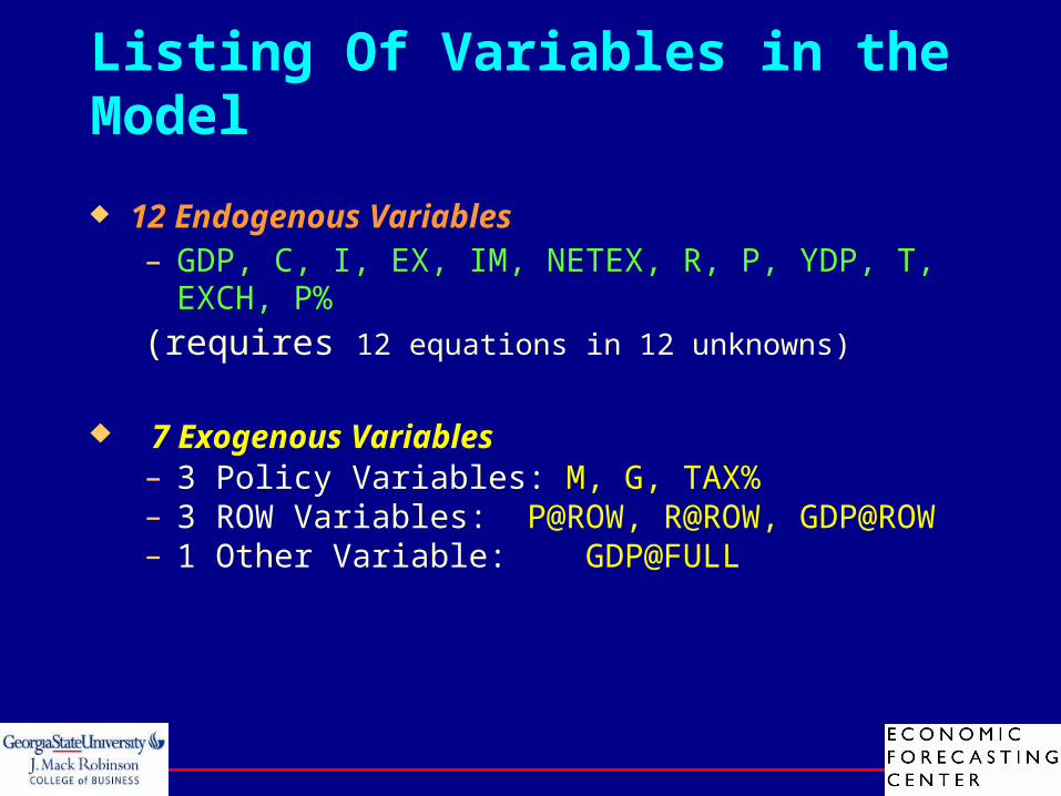
12 Endogenous Variables – GDP, C, I, EX, IM, NETEX, R, P, YDP, T, EXCH, P% (requires 12 equations in 12 unknowns)

7 Exogenous Variables– 3 Policy Variables: M, G, TAX%– 3 ROW Variables: P@ROW, R@ROW, GDP@ROW– 1 Other Variable: GDP@FULL

Listing Of Variables in the Model

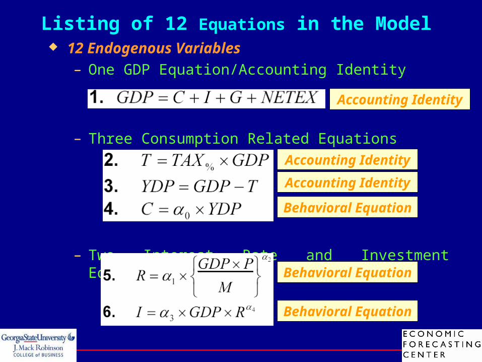
Listing of 12 Equations in the Model 12 Endogenous Variables

– One GDP Equation/Accounting Identity

– Three Consumption Related Equations

– Two Interest Rate and Investment Equations

Accounting Identity

Accounting Identity

Behavioral Equation

Behavioral Equation

Behavioral Equation

Accounting Identity

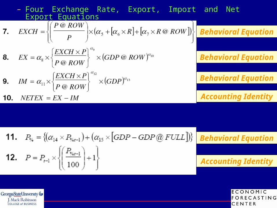
– Four Exchange Rate, Export, Import and Net Export Equations

– Two Price Inflation Equations

Accounting Identity

Accounting Identity

Behavioral Equation

Behavioral Equation

Behavioral Equation

Behavioral Equation

Glossary of Variables Type Variable Meaning Units

Endogenous C Consumption Billions of $

Endogenous EX Exports Billions of $

Endogenous EXCH Exchange Rate Index

Exogenous G Government Purchases Billions of $

Endogenous GDP Gross Domestic Product Billions of $

Exogenous GDP@FULL GDP @ Full Employment Billions of $

Exogenous GDP@ROW GDP in Rest of the World Billions of $

Endogenous I Investment Billions of $

Endogenous IM Imports Billions of $

Exogenous M Money supply Billions of $

Endogenous NETEX Net Exports Billions of $

Endogenous P Price Level Index

Endogenous P% Inflation Percent

Exogenous P@ROW Price Level, Rest of the

World

Index

Endogenous R Real Interest Rate Percent

Exogenous R@ROW Real Interest Rate, Rest of

the World

Percent

Endogenous T Tax Revenues Billions of $

Exogenous TAX% Tax Rate Fraction

Endogenous YDP Disposable Income Billions of $

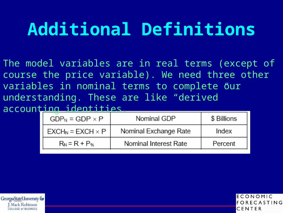
Additional Definitions

The model variables are in real terms (except of course the price variable). We need three other variables in nominal terms to complete our understanding. These are like “derived” accounting identities.

Econ 101 Rule

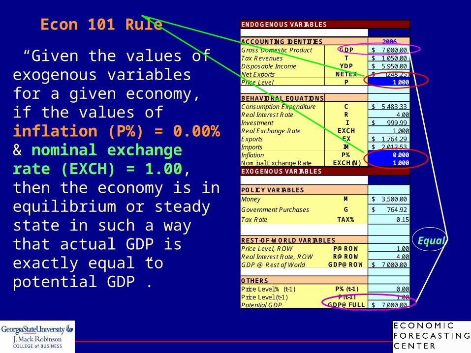
ENDOGENOUS VARIABLES

2006Gross Domestic Product GDP 7,000.00$ Tax Revenues T 1,050.00$ Disposable Income YDP 5,950.00$ Net Exports NETEX (248.25)$ Price Level P 1.000

BEHAVIORAL EQUATIONSConsumption Expenditure C 5,483.33$ Real Interest Rate R 4.00Investment I 999.99$ Real Exchange Rate EXCH 1.000Exports EX 1,764.29$ Imports IM 2,012.53$ Inflation P% 0.000Nominal Exchange Rate EXCH(N) 1.000EXOGENOUS VARIABLES

POLICY VARIABLES

Money M 3,500.00$

Government Purchases G 764.92$

Tax Rate TAX% 0.15

REST-OF-WORLD VARIABLESPrice Level, ROW P@ROW 1.00Real Interest Rate, ROW R@ROW 4.00GDP @ Rest of World GDP@ROW 7,000.00$

OTHERSPrice Level % (t-1) P%(t-1) 0.00Price Level (t-1) P(t-1) 1.00Potential GDP GDP@FULL 7,000.00$

ACCOUNTING IDENTITIES

Econ 101 Rule

“Given the values of exogenous variables for a given economy, if the values of inflation (P%) = 0.00% & nominal exchange rate (EXCH) = 1.00, then the economy is in equilibrium or steady state in such a way that actual GDP is exactly equal to potential GDP”.

Equal

Base Case

The Base Case is the state of the economy where for the given values of exogenous variables, the ECON 101 rule applies and the values of endogenous variables solved in the first year remain constant for all subsequent years

Base CaseThis means that GDP will be equal to its potential value for all the years in the base case.

Inflation will be equal to ZERO percent

And the exchange rate will be at one for all the years

Cont…

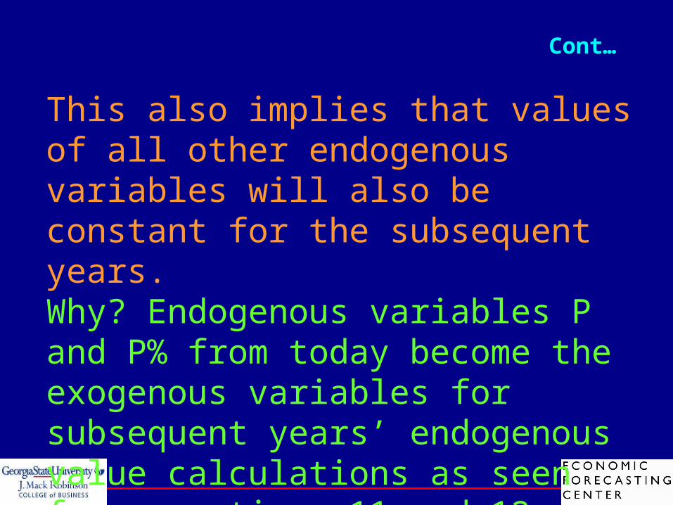
This also implies that values of all other endogenous variables will also be constant for the subsequent years.Why? Endogenous variables P and P% from today become the exogenous variables for subsequent years’ endogenous value calculations as seen from equations 11 and 12.

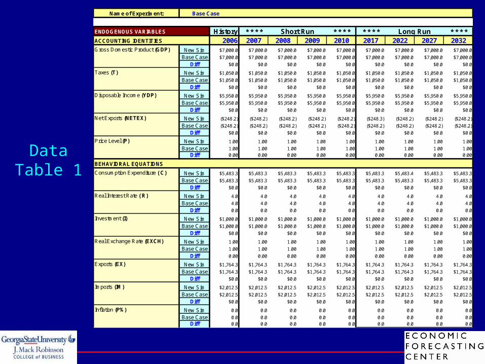
Data Table 1

Name of Experiment:

History * * * * * * * * * * * * * * * *2006 2007 2008 2009 2010 2017 2022 2027 2032

Gross Domestic Product (GDP) New Sim $7,000.0 $7,000.0 $7,000.0 $7,000.0 $7,000.0 $7,000.0 $7,000.0 $7,000.0 $7,000.0

Base Case $7,000.0 $7,000.0 $7,000.0 $7,000.0 $7,000.0 $7,000.0 $7,000.0 $7,000.0 $7,000.0

Diff $0.0 $0.0 $0.0 $0.0 $0.0 $0.0 $0.0 $0.0 $0.0

Taxes (T) New Sim $1,050.0 $1,050.0 $1,050.0 $1,050.0 $1,050.0 $1,050.0 $1,050.0 $1,050.0 $1,050.0

Base Case $1,050.0 $1,050.0 $1,050.0 $1,050.0 $1,050.0 $1,050.0 $1,050.0 $1,050.0 $1,050.0

Diff $0.0 $0.0 $0.0 $0.0 $0.0 $0.0 $0.0 $0.0 $0.0

Disposable Income (YDP) New Sim $5,950.0 $5,950.0 $5,950.0 $5,950.0 $5,950.0 $5,950.0 $5,950.0 $5,950.0 $5,950.0

Base Case $5,950.0 $5,950.0 $5,950.0 $5,950.0 $5,950.0 $5,950.0 $5,950.0 $5,950.0 $5,950.0

Diff $0.0 $0.0 $0.0 $0.0 $0.0 $0.0 $0.0 $0.0 $0.0

Net Exports (NETEX) New Sim ($248.2) ($248.2) ($248.2) ($248.2) ($248.2) ($248.3) ($248.2) ($248.2) ($248.2)

Base Case ($248.2) ($248.2) ($248.2) ($248.2) ($248.2) ($248.2) ($248.2) ($248.2) ($248.2)

Diff $0.0 $0.0 $0.0 $0.0 $0.0 $0.0 $0.0 $0.0 $0.0

Price Level (P) New Sim 1.00 1.00 1.00 1.00 1.00 1.00 1.00 1.00 1.00

Base Case 1.00 1.00 1.00 1.00 1.00 1.00 1.00 1.00 1.00Diff 0.00 0.00 0.00 0.00 0.00 0.00 0.00 0.00 0.00

BEHAVIORAL EQUATIONS

Consumption Expenditure ( C) New Sim $5,483.3 $5,483.3 $5,483.3 $5,483.3 $5,483.3 $5,483.3 $5,483.4 $5,483.3 $5,483.3

Base Case $5,483.3 $5,483.3 $5,483.3 $5,483.3 $5,483.3 $5,483.3 $5,483.3 $5,483.3 $5,483.3

Diff $0.0 $0.0 $0.0 $0.0 $0.0 $0.0 $0.0 $0.0 $0.0

Real Interest Rate ( R) New Sim 4.0 4.0 4.0 4.0 4.0 4.0 4.0 4.0 4.0

Base Case 4.0 4.0 4.0 4.0 4.0 4.0 4.0 4.0 4.0

Diff 0.0 0.0 0.0 0.0 0.0 0.0 0.0 0.0 0.0

Investment (I) New Sim $1,000.0 $1,000.0 $1,000.0 $1,000.0 $1,000.0 $1,000.0 $1,000.0 $1,000.0 $1,000.0

Base Case $1,000.0 $1,000.0 $1,000.0 $1,000.0 $1,000.0 $1,000.0 $1,000.0 $1,000.0 $1,000.0

Diff $0.0 $0.0 $0.0 $0.0 $0.0 $0.0 $0.0 $0.0 $0.0

Real Exchange Rate (EXCH) New Sim 1.00 1.00 1.00 1.00 1.00 1.00 1.00 1.00 1.00

Base Case 1.00 1.00 1.00 1.00 1.00 1.00 1.00 1.00 1.00

Diff 0.00 0.00 0.00 0.00 0.00 0.00 0.00 0.00 0.00

Exports (EX) New Sim $1,764.3 $1,764.3 $1,764.3 $1,764.3 $1,764.3 $1,764.3 $1,764.3 $1,764.3 $1,764.3

Base Case $1,764.3 $1,764.3 $1,764.3 $1,764.3 $1,764.3 $1,764.3 $1,764.3 $1,764.3 $1,764.3

Diff $0.0 $0.0 $0.0 $0.0 $0.0 $0.0 $0.0 $0.0 $0.0

Imports (IM) New Sim $2,012.5 $2,012.5 $2,012.5 $2,012.5 $2,012.5 $2,012.5 $2,012.5 $2,012.5 $2,012.5

Base Case $2,012.5 $2,012.5 $2,012.5 $2,012.5 $2,012.5 $2,012.5 $2,012.5 $2,012.5 $2,012.5

Diff $0.0 $0.0 $0.0 $0.0 $0.0 $0.0 $0.0 $0.0 $0.0

Inflation (P%) New Sim 0.0 0.0 0.0 0.0 0.0 0.0 0.0 0.0 0.0

Base Case 0.0 0.0 0.0 0.0 0.0 0.0 0.0 0.0 0.0Diff 0.0 0.0 0.0 0.0 0.0 0.0 0.0 0.0 0.0

ACCOUNTING IDENTITIES

Base Case

Long RunShort RunENDOGENOUS VARIABLES

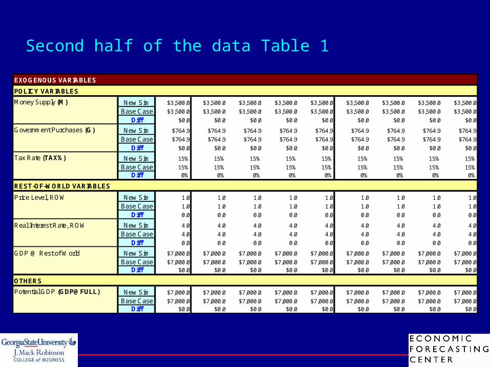
Second half of the data Table 1

EXOGENOUS VARIABLES

POLICY VARIABLES

Money Supply (M) New Sim $3,500.0 $3,500.0 $3,500.0 $3,500.0 $3,500.0 $3,500.0 $3,500.0 $3,500.0 $3,500.0

Base Case $3,500.0 $3,500.0 $3,500.0 $3,500.0 $3,500.0 $3,500.0 $3,500.0 $3,500.0 $3,500.0

Diff $0.0 $0.0 $0.0 $0.0 $0.0 $0.0 $0.0 $0.0 $0.0

Government Purchases (G) New Sim $764.9 $764.9 $764.9 $764.9 $764.9 $764.9 $764.9 $764.9 $764.9

Base Case $764.9 $764.9 $764.9 $764.9 $764.9 $764.9 $764.9 $764.9 $764.9

Diff $0.0 $0.0 $0.0 $0.0 $0.0 $0.0 $0.0 $0.0 $0.0

Tax Rate (TAX%) New Sim 15% 15% 15% 15% 15% 15% 15% 15% 15%

Base Case 15% 15% 15% 15% 15% 15% 15% 15% 15%Diff 0% 0% 0% 0% 0% 0% 0% 0% 0%

REST-OF-WORLD VARIABLES

Price Level, ROW New Sim 1.0 1.0 1.0 1.0 1.0 1.0 1.0 1.0 1.0

Base Case 1.0 1.0 1.0 1.0 1.0 1.0 1.0 1.0 1.0

Diff 0.0 0.0 0.0 0.0 0.0 0.0 0.0 0.0 0.0

Real Interest Rate, ROW New Sim 4.0 4.0 4.0 4.0 4.0 4.0 4.0 4.0 4.0

Base Case 4.0 4.0 4.0 4.0 4.0 4.0 4.0 4.0 4.0

Diff 0.0 0.0 0.0 0.0 0.0 0.0 0.0 0.0 0.0

GDP @ Rest of World New Sim $7,000.0 $7,000.0 $7,000.0 $7,000.0 $7,000.0 $7,000.0 $7,000.0 $7,000.0 $7,000.0

Base Case $7,000.0 $7,000.0 $7,000.0 $7,000.0 $7,000.0 $7,000.0 $7,000.0 $7,000.0 $7,000.0Diff $0.0 $0.0 $0.0 $0.0 $0.0 $0.0 $0.0 $0.0 $0.0

OTHERS

Potential GDP (GDP@FULL) New Sim $7,000.0 $7,000.0 $7,000.0 $7,000.0 $7,000.0 $7,000.0 $7,000.0 $7,000.0 $7,000.0

Base Case $7,000.0 $7,000.0 $7,000.0 $7,000.0 $7,000.0 $7,000.0 $7,000.0 $7,000.0 $7,000.0Diff $0.0 $0.0 $0.0 $0.0 $0.0 $0.0 $0.0 $0.0 $0.0

4 Important Guidelines to Use the Model

1. Tools/Options/Calculations/Iterations=100

2. Use Graph Button to Generate New Graphs for the experiment performed

3. Use Print Button for Printing the Results

4. To Reset the Model, Press the Base Case Button, and run the model once using the Calculations Button

Article: The Fed’s ThermostatWSJ: by: Milton Friedman

To keep prices stable, the Fed must see to it that the quantity of money changes in such a way as to offset movements in velocity and output

Keynes had taught them that the quantity of money did not matter, that what mattered was autonomous spending and the multiplier, that the role of monetary policy was to keep interest rates as low to promote investment and thereby full employment

Inflation, according to this vision was produced primarily by pressures on cost that could best be restrained by direct controls on prices and wages

MV = PY key a good thermostat was there all along