lecture 9: hidden markov modelsdprecup/courses/ml/lectures/ml-lecture... · example: robot position...

Lecture 9: Hidden Markov Models

• Working with time series data

• Hidden Markov Models

• Inference and learning problems

• Forward-backward algorithm

• Baum-Welch algorithm for parameter fitting

COMP-652 and ECSE-608, Lecture 9 - February 9, 2016 1

Time series/sequence data

• Very important in practice:

– Speech recognition– Text processing (taking into account the sequence of words)– DNA analysis– Heart-rate monitoring– Financial market forecasting– Mobile robot sensor processing– ...

• Does this fit the machine learning paradigm as described so far?

– The sequences are not all the same length (so we cannot just assumeone attribute per time step)

– The data at each time slice/index is not independent– The data distribution may change over time


Example: Robot position tracking1

Illustrative Example: Robot Localization

!"Prob

t=0Sensory model: never more than 1 mistake

Motion model: may not execute action with small prob.1From Pfeiffer, 2004


Example (II)Illustrative Example: Robot Localization

!"Prob

t=1


Example (III)


!"Prob

t=3


Example (IV)


!"Prob

t=4


Example (V)Illustrative Example: Robot Localization

! " # $

Trajectory

!%Prob

t=5


Hidden Markov Models (HMMs)

• Hidden Markov Models (HMMs) are used for situations in which:

– The data consists of a sequence of observations– The observations depend (probabilistically) on the internal state of a

dynamical system– The true state of the system is unknown (i.e., it is a hidden or latent

variable)

• There are numerous applications, including:

– Speech recognition– Robot localization– Gene finding– User modelling– Fetal heart rate monitoring– . . .


How an HMM works

• Assume a discrete clock t = 0, 1, 2, . . .

• At each t, the system is in some internal (hidden) state St = s and anobservation Ot = o is emitted (stochastically) based only on s(Random variables are denoted with capital letters)

• The system transitions (stochastically) to a new state St+1, accordingto a probability distribution P (St+1|St), and the process repeats.

• This interaction can be represented as a graphical model (recall thateach circle is a random variable, St or Ot in this case):

s1 s2 s3 s4

o1 o2 o3 o4

• Markov assumption: St+1⊥⊥St−1|St (future is independent of the pastgiven the present)


HMM definition

s1 s2 s3 s4

o1 o2 o3 o4

• An HMM consists of:

– A set of states S (usually assumed to be finite)– A start state distribution P (S1 = s),∀s ∈ S

This annotates the top left node in the graphical model– State transition probabilities: P (St+1 = s′|St = s),∀s, s′ ∈ S

These annotate the right-going arcs in the graphical model– A set of observations O (often assumed to be finite)– Observation emission probabilities P (Ot = o|St = s),∀s ∈ S, o ∈ O.

These annotate the down-going arcs above

• The model is homogeneous: the transition and emission probabilities donot depend on time, only on the states/observations


Finite HMMs

• If S and O are finite, the initial state distribution can be represented asa vector b0 of size |S|• Transition probabilities form a matrix T of size |S| × |S|; each row i is

the multinomial of the next state given that the current state is i• Similarly, the emission probabilities form a matrix Q of size |S| × |O|;

each row is a multinomial distribution over the observations, given thestate.• Together, b0, T and Q form the model of the HMM.• If O is not not finite, the multinomial can be replaced with an appropriate

parametric distribution (e.g. Normal)• If S is not finite, the model is usually not called an HMM, and different

ways of expressing the distributions may be used, e.g

– Kalman filter– Extended Kalman filter– ...


Examples

• Gene regulation

– O = {A,C,G, T}– S = {Gene,Transcription factor binding site, Junk DNA, . . . }

• Speech processing

– O = speech signal– S = word or phoneme being uttered

• Text understanding

– O = words– S = topic (e.g. sports, weather, etc)

• Robot localization

– O = sensor readings– S = discretized position of the robot


HMM problems

• How likely is a given observation sequence, o0, o1, . . . oT?I.e., compute P (O1 = o1, O2 = o2, . . . OT = oT )

• Given an observation sequence, what is the probability distribution forthe current state?I.e., compute P (ST = s|O1 = o1, O2 = o2, . . . OT = oT )

• What is the most likely state sequence for explaining a given observationsequence? (“Decoding problem”)

arg maxs1,...sT

P (S1 = s1, . . . ST = sT |O1 = o1, . . . OT = oT )

• Given one (or more) observation sequence(s), compute the modelparameters


Computing the probability of an observation sequence

• Very useful in learning for:

– Seeing if an observation sequence is likely to be generated by acertain HMM from a set of candidates (often used in classification ofsequences)

– Evaluating if learning the model parameters is working

• How to do it: belief propagation


Decomposing the probability of an observation sequence

s1 s2 s3 s4

o1 o2 o3 o4

P (o1, . . . oT ) =∑

s1,...sT

P (o1, . . . oT , s1, . . . sT )

=∑

s1,...sT

P (s1)

(T∏t=2

P (st|st−1)

)(T∏t=1

P (ot|st)

)(using the model)

=∑sT

P (oT |sT )∑

s1,...sT−1

P (sT |sT−1)P (s1)

(T−1∏t=2

P (st|st−1)

)(T−1∏t=1

P (ot|st)

)

This form suggests a dynamic programming solution!


Dynamic programming idea

• By inspection of the previous formula, note that we actually wrote:

P (o1, o2, . . . oT ) =∑sT

P (o1, o2, . . . oT , sT )

=∑sT

P (oT |sT )∑sT−1

P (sT |sT−1)P (o1, . . . oT−1, sT−1)

• The variables for the dynamic programming will be P (o1, o2, . . . ot, st).


The forward algorithm

• Given an HMM model and an observation sequence o1, . . . oT , define:

αt(s) = P (o1, . . . ot, St = s)

• We can put these variables together in a vector αt of size S.

• In particular,

α1(s) = P (o1, S1 = s) = P (o1|S1 = s)P (S1 = s) = qso1b0(s)

• For t = 2, . . . T, αt(s) = psot∑s′ ps′sαt−1(s

′)

• The solution is then

P (o1, . . . oT ) =∑s

αT (s)


Example

1 2 3 4 5

• Consider the 5-state hallway shown above

• The start state is always state 3

• The observation is the number of walls surrounding the state (2 or 3)

• There is a 0.5 probability of staying in the same state, and 0.25 probabilityof moving left or right; if the movement would lead to a wall, the stateis unchanged.

start to state see wallsstate 1 2 3 4 5 0 1 2 3 4

1 0.00 0.75 0.25 0.00 0.00 0.00 0.00 0.00 0.00 1.00 0.002 0.00 0.25 0.50 0.25 0.00 0.00 0.00 0.00 1.00 0.00 0.003 1.00 0.00 0.25 0.50 0.25 0.00 0.00 0.00 1.00 0.00 0.004 0.00 0.00 0.00 0.25 0.50 0.25 0.00 0.00 1.00 0.00 0.005 0.00 0.00 0.00 0.00 0.25 0.75 0.00 0.00 0.00 1.00 0.00


Example: Forward algorithm

1 2 3 4 5

Time t 1Obs 2αt(1) 0.00000αt(2) 0.00000αt(3) 1.00000αt(4) 0.00000αt(5) 0.00000



1 2 3 4 5

Time t 1 2Obs 2 2αt(1) 0.00000 0.00000αt(2) 0.00000 0.25000αt(3) 1.00000 0.50000αt(4) 0.00000 0.25000αt(5) 0.00000 0.00000


Example: Forward algorithm: two different observationsequences

1 2 3 4 5

Time t 1 2 3

Obs 2 2 2

αt(1) 0.00000 0.00000 0.00000

αt(2) 0.00000 0.25000 0.25000

αt(3) 1.00000 0.50000 0.37500

αt(4) 0.00000 0.25000 0.25000

αt(5) 0.00000 0.00000 0.00000

Time t 1 2 3

Obs 2 2 3

αt(1) 0.00000 0.00000 0.06250

αt(2) 0.00000 0.25000 0.00000

αt(3) 1.00000 0.50000 0.00000

αt(4) 0.00000 0.25000 0.00000

αt(5) 0.00000 0.00000 0.06250



1 2 3 4 5

Time t 1 2 3 4 5 6 7 8 9 10

Obs 2 2 3 2 3 2 2 2 3 3

αt(1) 0.0 0.00 0.0625 0.00000 0.00391 0.00000 0.00000 0.00000 0.00009 0.00007αt(2) 0.0 0.25 0.0000 0.01562 0.00000 0.00098 0.00049 0.00037 0.00000 0.00000αt(3) 1.0 0.50 0.0000 0.00000 0.00000 0.00000 0.00049 0.00049 0.00000 0.00000αt(4) 0.0 0.25 0.0000 0.01562 0.00000 0.00098 0.00049 0.00037 0.00000 0.00000αt(5) 0.0 0.00 0.0625 0.00000 0.00391 0.00000 0.00000 0.00000 0.00009 0.00007

• Note that probabilities decrease with the length of the sequence

• This is due to the fact that we are looking at a joint probability; thisphenomenon would not happen for conditional probabilities

• This can be a source of numerical problems for very long sequences.


Conditional probability queries in an HMM

• Because the state is never observed, we are often interested to infer itsconditional distribution from the observations.

• There are several interesting types of queries:

– Monitoring (filtering, belief state maintenance): what is the currentstate, given the past observations?

– Prediction: what will the state be in several time steps, given the pastobservations?

– Smoothing (hindsight): update the state distribution of past timesteps, given new data

– Most likely explanation: compute the most likely sequence of statesthat could have caused the observation sequence


Belief state monitoring

• Given an observation sequence o1, . . . ot, the belief state of an HMM attime step t is defined as:

bt(s) = P (St = s|o1, . . . ot)

Note that if S is finite bt is a probability vector of size S (so its elementssum to 1)

• In particular,

b1(s) = P (S1 = s|o1) =P (S1 = s, o1)

P (o1)=

P (S1 = s, o1)∑s′ P (S1 = s′, o1)

=b0(s)qso1∑s′ b0(s

′)qs′o1

• To compute this, we would assign:

b1(s)← b0(s)qso1

and then normalize it (dividing by∑s b1(s))


Updating the belief state after a new observation

s1 s2 s3 s4

o1 o2 o3 o4

• Suppose we have bt(s) and we receive a new observation ot+1. What isbt+1?

bt+1(s) = P (St+1 = s|o1, . . . otot+1) =P (St+1 = s, o1, . . . ot, ot+1)

P (o1, . . . ot, ot+1)

• The denominator is just a normalization constant, so we will work on thenumerator


Updating the belief state after a new observation (II)

s1 s2 s3 s4

o1 o2 o3 o4

bt+1(s) ∝ P (St+1 = s, o1, . . . ot, ot+1)

= P (ot+1|St+1 = s, o1, . . . ot)∑s′P (St+1 = s|St = s

′, o1, . . . ot)P (St = s

′, o1, . . . ot)

= P (ot+1|St+1 = s)∑s′P (St+1 = s|St = s

′)P (St = s

′, o1, . . . ot) (cond. independence)

∝ P (ot+1|St+1 = s)∑s′P (St+1 = s|St = s

′)P (St = s

′|o1, . . . ot)

= qsot+1

∑s′bt(s

′)ps′s (using notation)

Algorithmically, at every time step t, update:

bt+1(s)← qsot+1

∑s′

bt(s′)ps′s, then normalize


Computing state probabilities in general

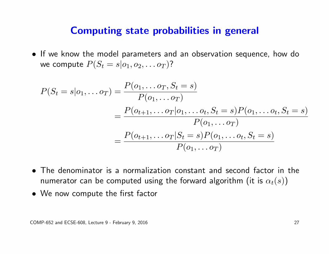
• If we know the model parameters and an observation sequence, how dowe compute P (St = s|o1, o2, . . . oT )?

P (St = s|o1, . . . oT ) =P (o1, . . . oT , St = s)

P (o1, . . . oT )

=P (ot+1, . . . oT |o1, . . . ot, St = s)P (o1, . . . ot, St = s)

P (o1, . . . oT )

=P (ot+1, . . . oT |St = s)P (o1, . . . ot, St = s)

P (o1, . . . oT )

• The denominator is a normalization constant and second factor in thenumerator can be computed using the forward algorithm (it is αt(s))

• We now compute the first factor


Computing state probabilities (II)

P (ot+1, . . . oT |St = s) =∑s′

P (ot+1, . . . oT , St+1 = s′|St = s)

=∑s′

P (ot+1, . . . oT |St+1 = s′, St = s)P (St+1 = s′|St = s)

=∑s′

P (ot+1|St+1 = s′)P (ot+2, . . . oT |St+1 = s′)P (St+1 = s′|St = s)

=∑s′

pss′qs′ot+1P (ot+2, . . . oT |St+1 = s′) (using notation)

• Define βt(s) = P (ot+1, . . . oT |St = s)• Then we can compute the βt by the following (backwards-in-time)

dynamic program:βT (s) = 1

βt(s) =∑s′

pss′qs′ot+1βt+1(s

′) for t = T − 1, T − 2, T − 3, . . .


The forward-backward algorithm

• Given the observation sequence, o1, . . . oT we can compute the probabilityof any state at any time as follows:

1. Compute all the αt(s), using the forward algorithm2. Compute all the βt(s), using the backward algorithm3. For any s ∈ S and t ∈ {1, . . . T}:

P (St = s|o1, . . . oT ) =P (o1, . . . ot, St = s)P (ot+1, . . . oT |St = s)

P (o1, . . . oT )=αt(s)βt(s)∑s′ αT (s

′)

• The complexity of the algorithm is O(|S|T ).• A similar dynamic programming approach can be used to compute the

most likely state sequence, given a sequence of observations:

arg maxs1,...sT

P (s1, . . . sT |o1, . . . oT )

This is called the Viterbi algorithm (see Rabiner tutorial)


Example: Forward-backward algorithm

1 2 3 4 5

Time t 1 2 3 4 5 6Obs 2 2 3 2 3 3βt(1) 0.00293 0.03516 0.04688 0.56250 0.75000 1.00000βt(2) 0.00586 0.01172 0.09375 0.18750 0.25000 1.00000βt(3) 0.00586 0.00000 0.09375 0.00000 0.00000 1.00000βt(4) 0.00586 0.01172 0.09375 0.18750 0.25000 1.00000βt(5) 0.00293 0.03516 0.04688 0.56250 0.75000 1.00000



1 2 3 4 5

Time t 1 2 3 4 5 6Obs 2 2 3 2 3 3αt(1) 0.00000 0.00000 0.06250 0.00000 0.00391 0.00293αt(2) 0.00000 0.25000 0.00000 0.01562 0.00000 0.00000αt(3) 1.00000 0.50000 0.00000 0.00000 0.00000 0.00000αt(4) 0.00000 0.25000 0.00000 0.01562 0.00000 0.00000αt(5) 0.00000 0.00000 0.06250 0.00000 0.00391 0.00293



1 2 3 4 5

Time t 1 2 3 4 5 6Obs 2 2 3 2 3 3P (St = 1|o1, . . . o6) 0.0 0.0 0.5 0.0 0.5 0.5P (St = 2|o1, . . . o6) 0.0 0.5 0.0 0.5 0.0 0.0P (St = 3|o1, . . . o6) 1.0 0.0 0.0 0.0 0.0 0.0P (St = 4|o1, . . . o6) 0.0 0.5 0.0 0.5 0.0 0.0P (St = 5|o1, . . . o6) 0.0 0.0 0.5 0.0 0.5 0.5


Learning HMM parameters

• Suppose we have access to observation sequences o1, . . . oT , and we knowthe state set S. How can we find the parameters λ = (pss′, qso, b0(s)) ofthe HMM that generated the observations?

• Usual optimization criterion: maximize the likelihood of the observeddata (we focus on this)

• Alternatively, in the Bayesian view, maximize the posterior probability ofthe observed data, given the prior over parameters

• Two main approaches:

– Baum-Welch algorithm (an instance of Expectation-Maximization forthe special case of HMM)

– Cheat! Get complete trajectories, s1, o1, s2, o2, . . . sT , oT and maximizeP (s1, o1, . . . sT , oT |λ)

• Some other, direct optimization approaches are also possible withcomplete data, but less popular


Learning with complete state information

• In many applications, we can make special arrangements to obtain stateinformation, at least for a few trajectories. For example:

– In speech recognition, human listeners can determine exactly whatword or phoneme is being spoken at each moment

– In gene identification, biological experiments can verify what parts ofthe DNA are actually genes

– In robot localization, we can collect data in a controlled environmentwhere the robot’s location is verified by other means (e.g., tapemeasure)

• Thus, at some extra (possibly high) cost, we can often obtain trajectoriesthat include the true system state: s1, o1, . . . sT , oT .

• It is much, much, much easier to train HMMs with such data than withobservation data alone!

• If there is little complete data, this approach can be used to initialize theparameters before Baum-Welch


Maximum likelihood learning with complete data in finiteHMM

• Suppose that we have a finite state set S and observation set O• Suppose we have a set of m trajectories, with the ith trajectory of the

form:τ i = (si1, o

i1, s

i2, o

i2, . . . s

iT i, o

iT i)

• Maximum likelihood estimates of the HMM parameters are:

b0(s) =# trajectories starting at s

m=|{i : si1 = s}|

m

pss′ =number of s-to-s′ transitions

number of occurrences of s=|{(i, t) : sit = s and sit+1 = s′}||{(i, t) : sit = s and t < T i}|

qso =number of times o was emitted in s

number of occurrences of s=|{(i, t) : sit = s and oit = o}|

|{(i, t) : sit = s}|


What if the observation space is infinite?

• An adequate parametric representation is chosen for the observationdistribution qs at each discrete state sE.g. Gaussian, exponential etc.

• The parameters of qs are then learned to maximize the likelihood of theobservation data associated with s

• E.g. for a Gaussian, we can compute the mean and covariance of theobservation vectors seen from each state s.


Example

1 2 3 4 5

• Data: one state-observation trajectory of 100 time steps

• Maximum likelihood model:start to state see walls

state 1 2 3 4 5 0 1 2 3 4

1 0.00 0.64 0.36 0.00 0.00 0.00 0.00 0.00 0.00 1.00 0.002 0.00 0.18 0.59 0.23 0.00 0.00 0.00 0.00 1.00 0.00 0.003 1.00 0.00 0.25 0.35 0.40 0.00 0.00 0.00 1.00 0.00 0.004 0.00 0.00 0.00 0.20 0.63 0.17 0.00 0.00 1.00 0.00 0.005 0.00 0.00 0.00 0.00 0.45 0.55 0.00 0.00 0.00 1.00 0.00

• Note that the emission model is correct but the transition model still haserrors compared to the true one, due to the limited amount of data

• In the limit, as t → ∞, the learned model would converge to the trueparameters


Maximum likelihood learning without state information

• Suppose we know O and S and they are finite

• Suppose we have a single observation trajectory o1, o2, . . . oT• We want to solve the following optimization problem:

max P (o1, . . . oT )

w.r.t. b0(s), pss′, qso

s.t. b0(s), pss′, qso ∈ [0, 1]∑s

b0(s) = 1

∑s′

pss′ = 1,∀s

∑o

qso = 1,∀s


Learning without state information: Baum-Welch

• The Baum-Welch algorithm is an Expectation-Maximization (EM)algorithm for fitting HMM parameters.

• Recall that EM is a general approach for dealing with missing data, byalternating two steps:

– “Fill in” the missing values based on the current model parameters– Re-compute the model parameters to maximize the likelihood of the

completed data

• For HMMs, the missing data is the state sequence, so we start withan initial guess about the model parameters and alternate the followingsteps:

– Estimate the probability of the state sequence given the observationsequence (using forward-backard algorithm)

– Fit new model parameters based on the completed data (using themaximum likelihood algorithm)


Baum-Welch algorithm

• Given observation sequence o1, . . . oT and initial parameters λ =(b0(s), pss′, qso)

• Repeat the following steps until convergence:

– E-Step:1. For every s, t compute: P (St = s|o1, . . . oT )2. For every s, s′, t compute: P (St = s, St+1 = s′|o1, . . . oT )

– M-Step:

b0(s) = P (S1 = s|o1, . . . oT )

pss′ =Expected # of s→ s′

Expected s occurences=

∑t<T P (St = s, St+1 = s′|o1, . . . oT )∑

t<T P (St = s|o1, . . . oT )

qso =Expected # o was emitted from s

Expected s occurrences=

∑t:ot=o

P (St = s|o1, . . . oT )∑tP (St = s|o1, . . . oT )


Details of E-Step

• P (St = s|o1, . . . oT ) is computed by the forward-backward algorithm.

• Recall: P (St = s, St+1 = s′|o1, . . . oT ) =P (St=s,St+1=s

′,o1,...oT )P (o1,...oT )

where

the denominator is∑sαT (s).

• Working on the numerator:

P (St = s, St+1 = s′, o1, . . . oT )

= P (St = s, o1, . . . ot)P (St+1 = s′, ot+1, . . . oT |St = s, o1, . . . ot)

= αt(s)P (St+1 = s′|St = s)P (ot+1, . . . oT |St+1 = s′)

= αt(s)pss′P (ot+1|St+1 = s′)P (ot+1, . . . oT |St+1 = s′)

= αt(s)pss′qs′ot+1βt+1(s

′)

where the α’s and β’s are from the forward-backward algorithm.


Remarks on Baum-Welch

• Each iteration increases P (o1, . . . oT ) (since this is EM)

• Each iteration is computationally efficient:

– E-step: O(|S|T ) for forward-backward, plus O(|S|2T ) for the secondestimation

– M-step: O(|S|2T ) plus O(|S||O|T ) for parameter estimation (giventhat we already have the αs and βs)

• Iterations are stopped when the parameters do not change much (or aftera fixed amount of time)

• The algorithm converges to a local maximum of the likelihood

• There can be many, many local maxima that are not globally optimal

• Reasonable initial guesses for parameters (obtained from prior knowledge,or from learning with a small amount of complete data) are a big help,but not a guarantee for good performance


Example: Baum-Welch from correct parameters

1 2 3 4 5Learned model:


1 0.00 0.59 0.41 0.00 0.00 0.00 0.00 0.00 0.00 1.00 0.002 0.00 0.35 0.01 0.65 0.00 0.00 0.00 0.00 1.00 0.00 0.003 1.00 0.00 0.20 0.60 0.20 0.00 0.00 0.00 1.00 0.00 0.004 0.00 0.00 0.00 0.65 0.01 0.35 0.00 0.00 1.00 0.00 0.005 0.00 0.00 0.00 0.00 0.41 0.59 0.00 0.00 0.00 1.00 0.00

Correct model:start to state see walls

state 1 2 3 4 5 0 1 2 3 4

1 0.00 0.75 0.25 0.00 0.00 0.00 0.00 0.00 0.00 1.00 0.002 0.00 0.25 0.50 0.25 0.00 0.00 0.00 0.00 1.00 0.00 0.003 1.00 0.00 0.25 0.50 0.25 0.00 0.00 0.00 1.00 0.00 0.004 0.00 0.00 0.00 0.25 0.50 0.25 0.00 0.00 1.00 0.00 0.005 0.00 0.00 0.00 0.00 0.25 0.75 0.00 0.00 0.00 1.00 0.00

Likelihood of data: 3.8645e-19


Example: Baum-Welch from equal initial parameters(uniform initial distributions)

1 2 3 4 5

• Learned model:start to state see walls

state 1 2 3 4 5 0 1 2 3 4

1 0.20 0.20 0.20 0.20 0.20 0.20 0.00 0.00 0.77 0.23 0.002 0.20 0.20 0.20 0.20 0.20 0.20 0.00 0.00 0.77 0.23 0.003 0.20 0.20 0.20 0.20 0.20 0.20 0.00 0.00 0.77 0.23 0.004 0.20 0.20 0.20 0.20 0.20 0.20 0.00 0.00 0.77 0.23 0.005 0.20 0.20 0.20 0.20 0.20 0.20 0.00 0.00 0.77 0.23 0.00

• Note that the learned model is really different from the true model

• Likelihood of data: 3.7977e-24


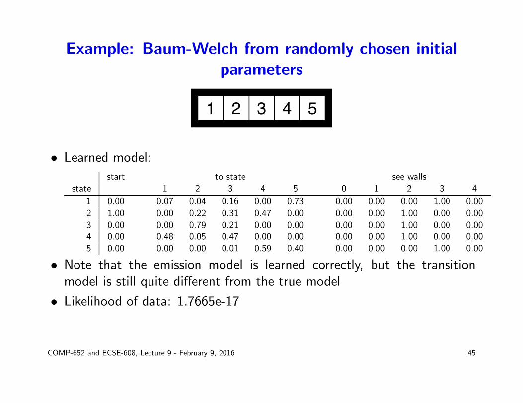
Example: Baum-Welch from randomly chosen initialparameters

1 2 3 4 5

• Learned model:


1 0.00 0.07 0.04 0.16 0.00 0.73 0.00 0.00 0.00 1.00 0.002 1.00 0.00 0.22 0.31 0.47 0.00 0.00 0.00 1.00 0.00 0.003 0.00 0.00 0.79 0.21 0.00 0.00 0.00 0.00 1.00 0.00 0.004 0.00 0.48 0.05 0.47 0.00 0.00 0.00 0.00 1.00 0.00 0.005 0.00 0.00 0.00 0.01 0.59 0.40 0.00 0.00 0.00 1.00 0.00

• Note that the emission model is learned correctly, but the transitionmodel is still quite different from the true model

• Likelihood of data: 1.7665e-17


The moral of the experiments

• The solution provided by EM can be arbitrarily different from the truemodel. Hence, interpreting the parameters learned by EM as having ameaning for the true problem is wrong

• Even when starting with the true model, EM may converge to somethingdifferent

• Some of the solutions provided by EM are useless (e.g. when startingwith uniform parameters)

• Choosing parameters at random is better than making them all equal,because it helps break symmetry

• A model with better likelihood is not necessarily closer to the true model(see training from the true model vs. training from a randomly chosenmodel)

• In general, in order to get EM to work, you either need a good initialmodel, or you need to do lots of random restarts


Learning the HMM structure

• All algorithms so far assume that we know the number of states

• If the number of states is not known, we can guess it and then learnparameters

• Note that the likelihood of the data usually increases with more states

• As a result, models with lots of states need to be penalized (usingregularization, minimum description length or a Bayesian prior over thenumber of states)

• If S is unknown, the algorithms work a lot worse


Application: Detection of DNA regions

• Observation: DNA sequence

• Hidden state: gene, transcription factor, protein-coding region...

• Learning: EM

• Validation often against known regions, and then through biologicalexperiment


Application: Music composition

• Observations: notes played

• States: chords

• Learning: music by one composer, labelled with correct chords, used formaximum likelihood learning

• Model ”composes” by sampling chords and notes from the model

• If successful, new music is generated “in the style” of the composer


Application: Speech recognition

• Observations: sound wave readings

• States: phonemes

• Learning: use labelled data to initialize the model, then EM with a muchlarger set of speakers to further adapt the parameters

• Transcription system: use inference to determine the most likely statesequence, which provides the transcription of the word

• HMMs are the state-of-art speech recognition technology

• Can be coupled with classification, if desired, to improve recognitionperformance


Application: Classification of time series

• Use one HMM for each class, and learn its parameters from data

• When given a new observation sequence, compute its likelihood undereach HMM

• The example is assigned the label of the class that yields the highestlikelihood


Summary

• Hidden Markov Models formalize sequential observation of a systemwithout perfect access to state (i.e., state is “hidden”)

• A variety of inference problems can be solved using straightforwarddynamic programming algorithms

• The learning (parameter fitting) problem is best done with “supervised”data – i.e., state & observation trajectories

• Parameter fitting can also be solved purely from observation data usingEM (called the Baum-Welch algorithm), but results are only locallyoptimal

• EM can behave in strange ways, so getting it to work may take effort

• Lots of applications!


lecture 9: hidden markov modelsdprecup/courses/ml/lectures/ml-lecture... · example: robot position...

Documents