mapped elements and numerical 'singularity' …freeit.free.fr/finite...

Mapped elements and numerical integration - 'infinite' and

'singularity' elements

9.1 Introduction In the previous chapter we have shown how some general families of finite elements can be obtained for Co interpolations. A progressively increasing number of nodes and hence improved accuracy characterizes each new member of the family and presumably the number of such elements required to obtain an adequate solution decreases rapidly. To ensure that a small number of elements can represent a relatively complex form of the type that is liable to occur in real, rather than academic, problems, simple rectangles and triangles no longer suffice. This chapter is therefore concerned with the subject of distorting such simple forms into others of more arbitrary shape.

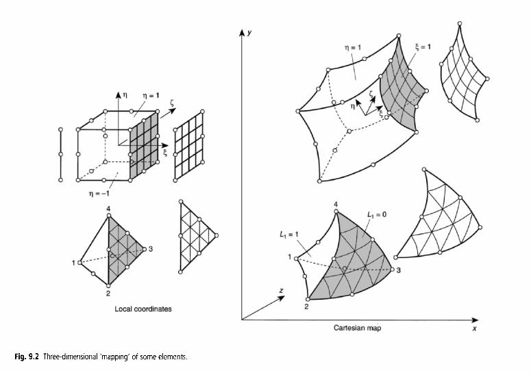
Elements of the basic one-, two-, or three-dimensional types will be 'mapped' into distorted forms in the manner indicated in Figs 9.1 and 9.2.

In these figures it is shown that the <, q, [, or L1 L2L3L4 coordinates can be distorted to a new, curvilinear set when plotted in Cartesian x, y , z space.

Not only can two-dimensional elements be distorted into others in two dimensions but the mapping of these can be taken into three dimensions as indicated by the flat sheet elements of Fig. 9.2 distorting into a three-dimensional space. This principle applies generally, providing a one-to-one correspondence between Cartesian and curvilinear coordinates can be established, i.e., once the mapping relations of the type

f X ( < l % 0 f x ( L 1 , L 2 i L 3 , L 4 ) {I} = { 2i::::::i 1 Or { 2:::::;:::;::; 1 (9.1)

can be established. Once such coordinate relationships are known, shape functions can be specified in

local coordinates and by suitable transformations the element properties established in the global coordinate system.

In what follows we shall first discuss the so-called isoparametric form of relationship (9.1) which has found a great deal of practical application. Full details of this formulation will be given, including the establishment of element matrices by numerical integration.

vi c

c

a,

-

G g a,

a - 0 0,

c

Q

Q

.-

-2 ._

E x 2

-

IT)

CZ 0

c

.- VI

- oi d, .- L

L

Use of ‘shape functions’ in the establishment of coordinate transformations 203

In the final section we shall show that many other coordinate transformations can be used effectively.

Pa ram et r i c c u rvi I i near coo r d i nates

9.2 Use of ‘shape functions’ in the establishment of coordinate transformations

A most convenient method of establishing the coordinate transformations is to use the ‘standard’ type of Co shape functions we have already derived to represent the variation of the unknown function.

If we write, for instance, for each element

x = Nix’ + Nix2 + . . . = N’ { !:} = N’x

in which N’ are standard shape functions given in terms of the local coordinates, then a relationship of the required form is immediately available. Further, the points with coordinates xl , y l , zl , etc., will lie at appropriate points of the element boundary (as from the general definitions of the standard shape functions we know that these have a value of unity at the point in question and zero elsewhere). These points can establish nodes a priori.

To each set of local coordinates there will correspond a set of global Cartesian coordinates and in general only one such set. We shall see, however, that a non-uniqueness may arise sometimes with violent distortion.

The concept of using such element shape functions for establishing curvilinear coordinates in the context of finite element analysis appears to have been first introduced by Taig.’ In his first application basic linear quadrilateral relations were used. iron^^.^ generalized the idea for other elements.

Quite independently the exercises of devising various practical methods of generat- ing curved surfaces for purposes of engineering design led to the establishment of similar definitions by Coons4 and Forrest,’ and indeed today the subjects of surface definitions and analysis are drawing closer together due to this activity.

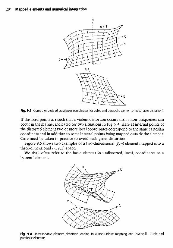
In Fig. 9.3 an actual distortion of elements based on the cubic and quadratic members of the two-dimensional ‘serendipity’ family is shown. It is seen here that a one-to-one relationship exists between the local ( E , 7 ) and global (x, y ) coordinates.

204 Mapped elements and numerical integration

Fig. 9.3 Computer plots of curvilinear coordinates for cubic and parabolic elements (reasonable distortion).

If the fixed points are such that a violent distortion occurs then a non-uniqueness can occur in the manner indicated for two situations in Fig. 9.4. Here at internal points of the distorted element two or more local coordinates correspond to the same Cartesian coordinate and in addition to some internal points being mapped outside the element. Care must be taken in practice to avoid such gross distortion.

Figure 9.5 shows two examples of a two-dimensional ( 6 , ~ ) element mapped into a three-dimensional (x, y , z ) space.

We shall often refer to the basic element in undistorted, local, coordinates as a 'parent' element.

- Fig. 9.4 Unreasonable element distortion leading to a non-unique mapping and 'overspill'. Cubic and parabolic elements.

Use of 'shape functions' in the establishment of coordinate transformations 205

Fig. 9.5 Flat elements (of parabolic type) mapped into three-dimensions,

In Sec. 9.5 we shall define a quantity known as the jacobian determinant. The well- known condition for a one-to-one mapping (such as exists in Fig. 9.3 and does not in Fig. 9.4) is that the sign of this quantity should remain unchanged at all the points of the mapped element.

It can be shown that with a parametric transformation based on bilinear shape functions, the necessary condition is that no internal angle [such as a in Fig. 9.6(a)]

Fig. 9.6 Rules for uniqueness of mapping (a) and (b).


be greater than 1 800.6 In transformations based on parabolic-type ‘serendipity’ functions, it is necessary in addition to this requirement to ensure that the mid-side nodes are in the ‘middle half of the distance between adjacent corners but a ‘middle third’ shown in Fig. 9.6 is safer. For cubic functions such general rules are impractical and numerical checks on the sign of the jacobian determinant are necessary. In practice a parabolic distortion is usually sufficient.

9.3 Geometrical conformability of elements While it was shown that by the use of the shape function transformation each parent element maps uniquely a part of the real object, it is important that the subdivision of this into the new, curved, elements should leave no gaps. The possibility of such gaps is indicated in Fig. 9.7.

Fig. 9.7 Compatibility requirements in a real subdivision of space.

Theorem 1. r f two adjacent elements are generated from ‘parents’ in which the shape functions satisfy C, continuity requirements then the distorted elements will be contig- uous (compatible).

This theorem is obvious, as in such cases uniqueness of any function u required by continuity is simply replaced by that of uniqueness of the x, y , or z coordinate. As adjacent elements are given the same sets of coordinates at nodes, continuity is implied.

9.4 Variation of the unknown function within distorted, curvilinear elements. Continuity requirements

With the shape of the element now defined by the shape functions N’ the variation of the unknown, u, has to be specified before we can establish element properties. This is

Variation of the unknown function within distorted, curvilinear elements 207

. .

Fig. 9.8 Various element specifications: 0 point at which coordinate is specified; 0 points at which the function parameter is specified. (a) Isoparametric, (b) superparametric, (c) subparametric.

most conveniently given in terms of local, curvilinear coordinates by the usual expression

where ae lists the nodal values.

Theorem 2. If the shape functions N used in (9.3) are such that Co continuity of u is preserved in the parent coordinates then C, continuity requirements will be satisfied in distorted elements.

u = Nae (9.3)

The proof of this theorem follows the same lines as that in the previous section. The nodal values may or may not be associated with the same nodes as used to

specify the element geometry. For example, in Fig. 9.8 the points marked with a circle are used to define the element geometry. We could use the values of the function defined at nodes marked with a square to define the variation of the unknown.

In Fig. 9.8(a) the same points define the geometry and the finite element analysis points. If then

N = N’ (9.4) i.e., the shape functions defining the geometry and the function are the same, the elements will be called isoparametric.

We could, however, use only the four corner points to define the variation of u [Fig. 9.8(b)]. We shall refer to such an element as superparametric, noting that the variation of geometry is more general than that of the actual unknown.

Similarly, if for instance we introduce more nodes to define u than are used to define the geometry, subparametric elements will result [Fig. 9.8(c)].


While for mapping it is convenient to use ‘standard’ forms of shape functions the interpolation of the unknown can, of course, use hierarchic forms defined in the previous chapter. Once again the definitions of sub- and superparametric variations are applicable.

Transformations

9.5 Evaluation of element matrices (transformation in E,, q, ( coordinates)

To perform finite element analysis the matrices defining element properties, e.g., stiffness, etc., have to be found. These will be of the form

JvGdV (9.5)

Jv BTDB d V (9.6)

in which the matrix G depends on N or its derivatives with respect to global coordinates. As an example of this we have the stiffness matrix

and associated body force vectors

J NTbdV V

(9-7)

For each particular class of elastic problems the matrices of B are given explicitly by their components [see the general form of Eqs (4.10), (5.6), and (6.1 l)]. Quoting the first of these, Eq. (4. IO), valid for plane problems we have

In elasticity problems the matrix G is thus a function of the first derivatives of N and this situation will arise in many other classes of problem. In all, C,, continuity is needed and, as we have already noted, this is readily satisfied by the functions of Chapter 8, written now in terms of curvilinear coordinates.

To evaluate such matrices we note that two transformations are necessary. In the first place, as Ni is defined in terms of local (curvilinear) coordinates, it is necessary to devise some means of expressing the global derivatives of the type occurring in Eq. (9.8) in terms of local derivatives.

In the second place the element of volume (or surface) over which the integration has to be carried out needs to be expressed in terms of the local coordinates with an appropriate change of limits of integration.

Evaluation of element matrices (transformation in 5, q, 5 coordinates) 209

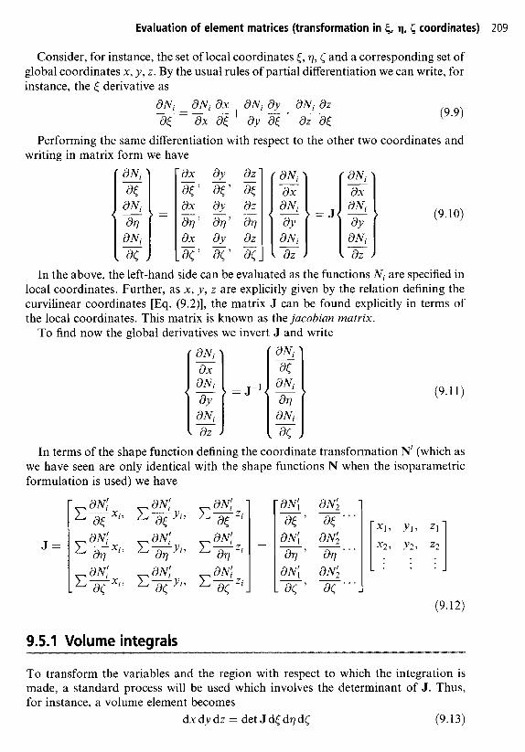
Consider, for instance, the set of local coordinates (, 71, < and a corresponding set of global coordinates x, y , z . By the usual rules of partial differentiation we can write, for instance, the < derivative as

Performing the same differentiation with respect to the other two coordinates and writing in matrix form we have

(9.10)

In the above, the left-hand side can be evaluated as the functions N; are specified in local coordinates. Further, as x, y , z are explicitly given by the relation defining the curvilinear coordinates [Eq. (9.2)], the matrix J can be found explicitly in terms of the local coordinates. This matrix is known as the jucobiun matrix.

To find now the global derivatives we invert J and write

dN; d X dN; dY dN; dZ

~

-

-

> (9.11)

In terms of the shape function defining the coordinate transformation N’ (which as we have seen are only identical with the shape functions N when the isoparametric formulation is used) we have

XI ’ X2’

Y l ,

Y2,

(9.12)

9.5.1 Volume integrals

To transform the variables and the region with respect to which the integration is made, a standard process will be used which involves the determinant of J. Thus, for instance, a volume element becomes

dxdydz = detJdJdqd< (9.13)


This type of transformation is valid irrespective of the number of coordinates used. For its justification the reader is referred to standard mathematical texts.t (See also Appendix F.)

Assuming that the inverse of J can be found we now have reduced the evaluation of the element properties to that of finding integrals of the form of Eq. (9.5).

More explicitly we can write this as

(9.14)

if the curvilinear coordinates are of the normalized type based on the right prism. Indeed the integration is carried out within such a prism and not in the complicated distorted shape, thus accounting for the simple integration limits. One- and two- dimensional problems will similarly result in integrals with respect to one or two coordinates within simple limits.

While the limits of integration are simple in the above case, unfortunately the explicit form of G is not. Apart from the simplest elements, algebraic integration usually defies our mathematical skill, and numerical integration has to be used. This, as will be seen from later sections, is not a severe penalty and has the advantage that algebraic errors are more easily avoided and that general programs, not tied to a particular element, can be written for various classes of problems. Indeed in such numerical calculations the analytical inverses of J are never explicitly found.

9.5.2 Surface integrals In elasticity and other applications, surface integrals frequently occur. Typical here are the expressions for evaluating the contributions of surface tractions [see Chapter 2, Eq. (2.24b)l:

f = - NTidA

The element dA will generally lie on a surface where one of the coordinates (say C) is constant.

The most convenient process of dealing with the above is to consider dA as a vector oriented in the direction normal to the surface (see Appendix F). For three- dimensional problems we form the vector product

J A

and on substitution integrate within the domain - 1 < E , 7 d 1

written as +The determinant of the jacobian matrix is known in the literature simply as 'the jacobian' and is often

Element matrices. Area and volume coordinates 21 1

For two dimensions a line length dS arises and here the magnitude is simply

on constant 7 surfaces. This may now be reduced to two components for the two- dimensional problem.

9.6 Element matrices. Area and volume coordinates The general relationship (9.2) for coordinate mapping and indeed all the following theorems are equally valid for any set of local coordinates and could relate the local Ll , Lz, . . . coordinates used for triangles and tetrahedra in the previous chapter, to the global Cartesian ones.

Indeed most of the discussion of the previous chapter is valid if we simply rename the local coordinates suitably. However, two important differences arise.

The first concerns the fact that the local coordinates are not independent and in fact number one more than the Cartesian system. The matrix J would apparently therefore become rectangular and would not possess an inverse. The second is simply the difference of integration limits which have to correspond with a triangular or tetrahedral ‘parent’.

The simplest, though perhaps not the most elegant, way out of the first difficulty is to consider the last variable as a dependent one. Thus, for example, we can introduce formally, in the case of the tetrahedra,

< = L ,

7 = L2

I = L3 (9.15)

l - C - v - < = L 4

(by definition in the previous chapter) and thus preserve without change Eq. (9.9) and all the equations up to Eq. (9.14).

As the functions Ni are given in fact in terms of L 1 , L2, etc., we must observe that

(9.16) ~ dN; - --+22+-3+-- dNi dL1 d N . dL dN, dL dNi dL4

- a< dL1 a< dL2 a< dL3 d[ dL4 a< On using Eq. (9.15) this becomes simply

6”; - dNi dN, ~ - 86 d~~ aL4

with the other derivatives obtainable by similar expressions.

21 2 Mapped elements and numerical integration

- 1 0 0

0 1 0

0 0 1

0 0 0 -

The integration limits of Eq. (9.14) now change, however, to correspond with the tetrahedron limits, typically

-

(9.17)

The same procedure will clearly apply in the case of triangular coordinates. It must be noted that once again the expression G will necessitate numerical

integration which, however, is carried out over the simple, undistorted, parent region whether this be triangular or tetrahedral.

An alternative to the above is to express the coordinates and constraint as

rx = x - x1 N{ - x2N4 - x3N; - . . . = 0

ry = y - ylNi - y2N4 -y3N; - ... = 0

r Z = z - z z l N i - z 2 N i - z 3 N i - . . . = 0

rl = 1 - L1 - L2 - L3 - L4 = O

(9.18)

where N: = N’(L1, L2, L3, L4) , etc. Now derivatives of the above with respect to x and y may be written directly as

dr,y ar, drx _ _ _ ax ay az ary dry dry _ _ _ a x ay az

X

1 1 1 1

a~~ a~~ aL2 a x ay az

a~~ a~~ a~~ a x ay az

- - -

_ _ - -

a~~ a~~ a~~ a x ay az p-p

= o (9.19)

The above may be solved for the partial derivatives of L , with respect to the x , y , z coordinates and used directly with the chain rule written as

aNj aN, aLi aN, d L aNi dL3 aN; dL4 - - - -.p+p2+pp+p- (19.20)

The above has advantages when the coordinates are written using mapping functions as the computation can still be more easily carried out. Also, the calculation of integrals will normally be performed numerically (as described in Sec. 9.10) where the points for integration are defined directly in terms of the volume coordinates.

ax a ~ , a x a ~ ? , ax a~~ ax a~~ ax

Convergence of elements in curvilinear coordinates 21 3

Fig. 9.9 A distorted triangular prism.

Finally it should be remarked that any of the elements given in the previous chapter are capable of being mapped. In some, such as the triangular prism, both area and rectangular coordinates are used (Fig. 9.9). The remarks regarding the dependence of coordinates apply once again with regard to the former but the processes of the present section should make procedures clear.

9.7 Convergence of elements in curvilinear coordinates To consider the convergence aspects of the problem posed in curvilinear coordinates it is convenient to return to the starting point of the approximation where an energy functional ll, or an equivalent integral form (Galerkin problem statement), was defined by volume integrals essentially similar to those of Eq. ( 9 3 , in which the integrand was a function of u and its first derivatives.

Thus, for instance, the variational principles of the energy kind discussed in Chapter 2 (or others of Chapter 3) could be stated for a scalar function u as

(9.21)

The coordinate transformation changes the derivatives of any function by the jacobian relation (9.1 1). Thus

> (9.22)

and the functional can be stated simply by a relationship of the form (9.21) with x , y , etc., replaced by E , 7, etc., with the maximum order of differentiation unchanged.

It follows immediately that if the shape functions are chosen in curvilinear coordinate space so as to observe the usual rules of convergence (continuity and presence of complete first-order polynomials in these coordinates), then convergence will occur. Further, all the arguments concerning the order of convergence with the element size h still hold, providing the solution is related to the curvilinear coordinate system.

Indeed, all that has been said above is applicable to problems involving higher derivatives and to most unique coordinate transformations. It should be noted that


the patch test as conceived in the x , y , . . . coordinate system (see Chapters 2 and 10) is no longer simply applicable and in principle should be applied with polynomial fields imposed in the curvilinear coordinates. In the case of isoparametric (or subparametric) elements the situation is more advantageous. Here a linear (constant derivative x , y ) field is always reproduced by the curvilinear coordinate expansion, and thus the lowest order patch test will be passed in the standard manner on such elements.

The proof of this is simple. Consider a standard isoparametric expansion

u = Niai FE Na N = N((,q, <) i = 1

with coordinates of nodes defining the transformation as

x = Nixi y = Nivi z = Nizi

(9.23)

(9.24)

The question is under what circumstances is it possible for expression (9.23) to define a linear expansion in Cartesian coordinates:

u = a1 + a 2 ~ + c ~ 3 y + a 4 2

= a1 + a2 Nixi + a3 Niy i + a4 Nizi (9.25)

If we take ai = a1 + a2xi + a3yi + a4zi

and compare expression (9.23) with (9.25) we note that identity is obtained between these providing

X N i = l

As this is the usual requirement of standard element shape functions [see Eq. (8.4)] we can conclude that the following theorem is valid.

Theorem 3. The constant derivative condition will be satisjied for all isoparametric elements.

As subparametric elements can always be expressed as specific cases of an isoparametric transformation this theorem is obviously valid here also.

It is of interest to pursue the argument and to see under what circumstances higher polynomial expansions in Cartesian coordinates can be achieved under various transformations. The simple linear case in which we ‘guessed’ the solution has now to be replaced by considering in detail the polynomial terms occurring in expressions such as (9.23) and (9.25) and establishing conditions for equating appropriate coefficients.

Consider a specific problem: the circumstances under which the bilinearly mapped quadrilateral of Fig. 9.10 can fully represent any quadratic Cartesian expansion. We now have

A A

x = N ; X ~ y = Njy; (9.26) 1 1

(9.27)

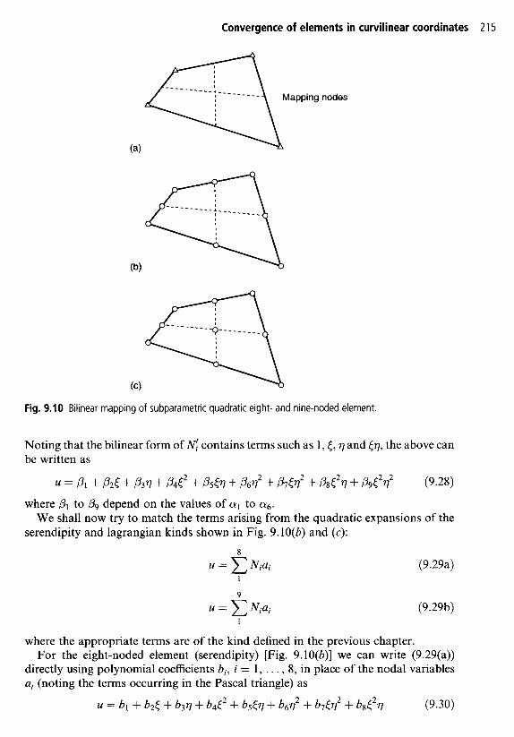
Convergence of elements in curvilinear coordinates 21 5

Fig. 9.10 Bilinear mapping of subparametric quadratic eight- and nine-noded element.

Noting that the bilinear form of Ni contains terms such as 1, E , q and Eq, the above can be written as

2.4 = PI + P2E -k P3q + p4t2 + P55.I + P6q2 + Pdq2 + P852q f P9E2q2 (9.28)

where PI to p9 depend on the values of a1 to (Y6.

serendipity and lagrangian kinds shown in Fig. 9.10(b) and (c): We shall now try to match the terms arising from the quadratic expansions of the

8

u = C Nisi (9.29a) 1

9

u = C N ; u ~ (9.29b) 1

where the appropriate terms are of the kind defined in the previous chapter. For the eight-noded element (serendipity) [Fig. 9.10(b)] we can write (9.29(a))

directly using polynomial coefficients bi, i = 1, . . . , 8, in place of the nodal variables ai (noting the terms occurring in the Pascal triangle) as

u = bl + b2< + b3q + b4E2 + b5Jq + b6T2 + b7[q2 + b8t2q (9.30)


Fig. 9.1 1 Quadratic serendipity and Lagrange eight- and nine-noded elements in regular and distorted form. Elastic deflection of a beam under constant moment. Note the poor results of the eight-noded element.

It is immediately evident that for arbitrary values of p1 to p9 it is impossible to match the coefficients bl to b8 due to the absence of the term E2v2 in Eq. (9.30). [However if higher order (quartic, etc.) expansions of the serendipity kind were used such matching would evidently be possible and we could conclude that for

Numerical integration - one-dimensional 2 17

linearly distorted elements the serendipity family of order four or greater will always represent quadratics.]

For the nine-noded, lagrangian, element [Fig. 9.10(c)] the expansion similar to (9.30) gives

(9.31)

and the matching of the coefficients of Eqs (9.3 1) and (9.28) can be made directly. We can conclude therefore that nine-noded elements represent better Cartesian

polynomials (when distorted linearly) and therefore are generally preferable in modelling smooth solutions. This matter was first presented by Wachspress but the simple proof presented above is due to Crochet.8 An example of this is given in Fig. 9.11 where we consider the results of a finite element calculation with eight- and nine-noded elements respectively used to reproduce a simple beam solution in which we know that the exact answers are quadratic. With no distortion both elements give exact results but when distorted only the nine-noded element does so, with the eight-noded element giving quite wild stress fluctuation.

Similar arguments will lead to the conclusion that in three dimensions again only the lagrangian 27-noded element is capable of reproducing fully the quadratic in Cartesian coordinates when trilinearly distorted.

Lee and Bathe’ investigate the problem for cubic and quartic serendipity and lagrangian quadrilateral elements and show that under bilinear distortions the full order Cartesian polynomial terms remain in Lagrange elements but not in serendipity ones. They also consider edge distortion and show that this polynomial order is always lost. Additional discussion of such problems is also given by Wach~press .~

u = bl + b2< + b3v + b4E2 + . . . + bgE2v + bgJ2v2

9.8 Numerical integration - one-dimensional In Chapter 5, dealing with a relatively simple problem of axisymmetric stress distribu- tion and simple triangular elements, it was noted that exact integration of expressions for element matrices could be troublesome. Now for the more complex distorted elements numerical integration is essential.

Some principles of numerical integration will be summarized here together with tables of convenient numerical coefficients.

To find numerically the integral of a function of one variable we can proceed in one of several ways.”

9.8.1 Newton-Cotes quadrature!

In the most obvious procedure, points at which the function is to be found are determined a priori - usually at equal intervals - and a polynomial passed through the values of the function at these points and exactly integrated [Fig. 9.12(a)].

t ‘Quadrature’ is an alternative term to ‘numerical integration’.


. .

Fig. 9.1 2 (a) Newton-Cotes and (b) Gauss integrations. Each integrates exactly a seventh-order polynomial [i.e., error 0(h8) ] .

As n values of the function define a polynomial of degree n - 1, the errors will be of the order O(h“) where h is the element size. This leads to the well-known Newton-Cotes ‘quadrature’ formulae. The intregrals can be written as

Z = J’ f ( < ) d< = 2 Hif(<ii) (9.32)

for the range of integration between - 1 and +1 [Fig. 9.12(a)]. For example, if n = 2, we have the well-known trapezoidal rule:

1

-1 1

I =f(-1) + f ( l ) (9.33)

(9.34)

for n = 3 , the Simpson ‘one-third’ rule:

I = 4 Lf -1 ) + 4 f W + f ( l ) l

Numerical integration - rectangular (2D) or right prism (3D) regions 219

and for n = 4:

I = arfc-1, + 3f(-4) + 3f($ + f ( l ) l (9.35)

Formulae for higher values of n are given in reference 10.

9.8.2 Gauss quadrature

If in place of specifying the position of sampling points apriori we allow these to be loca- ted at points to be determined so as to aim for best accuracy, then for a given number of sampling points increased accuracy can be obtained. Indeed, if we again consider

(9.36)

and again assume a polynomial expression, it is easy to see that for n sampling points we have 2n unknowns (Hi and ti) and hence a polynomial of degree 2n - 1 could be constructed and exactly integrated [Fig. 9.12(b)]. The error is thus of order 0 ( h z n ) .

The simultaneous equations involved are difficult to solve, but some mathematical manipulation will show that the solution can be obtained explicitly in terms of Legendre polynomials. Thus this particular process is frequently known as Gauss- Legendre quadrature."

Table 9.1 shows the positions and weighting coefficients for gaussian integration. For purposes of finite element analysis complex calculations are involved in deter-

mining the values off, the function to be integrated. Thus the Gauss-type processes, requiring the least number of such evaluations, are ideally suited and from now on will be used exclusively.

Other expressions for integration of functions of the type

(9.37)

can be derived for prescribed forms of w(<), again integrating up to a certain order of accuracy a polynomial expansion off(<). lo

9.9 Numerical integration - rectangular (2D) or right prism (3D) regions

The most obvious way of obtaining the integral

is to first evaluate the inner integral keeping 77 constant, i.e.,

(9.38)

(9.39)


Table 9.1 Abscissae and weight coefficients of the gaussian quadrature formula Jllf(x) dx = Cy=l H i f ( a i )

f a

0

1/&

m 0.000 000 000 000 000

0.861 136311 594953 0.339 981 043 584 856

0.906 179 845 938 664 0.538469310 105683 0.000 000 000 000 000

0.932469 514203 152 0.661 209 386466265 0.238619 186083 197

0.949 107912342759 0.741 531 185599394 0.405845 151 377 397 0.000 000 000 000 000

0.960 289 856 497 536 0.796666477413 627 0.525 532409916329 0.183 434 642 495 650

0.968 160239507 626 0.836031 107326636 0.613371432700590 0.324 253 423 403 809 0.000 000 000 000 000

0.973 906 528 5 17 172 0.865 063 366 688 985 0.679 409 568 299 024 0.433 395 394 129 247 0.148 874 338 981 631

n = l

n = 2

n = 3

n = 4

n = 5

n = 6

n = 7

n = 8

n = 9

n = 10

H

2.000 000 000 000 000

1 .ooo 000 000 000 000

519 519

0.347854845 137454 0.652 145 154 862 546

0.236 926 885 056 189 0.478 628 670 499 366 0.568 888 888 888 889

0.171 324492379 170 0.360761 573048 139 0.467913934572 691

0.129484966 168 870 0.279 705 391 489 277 0.381 830050505 119 0.417959 183673469

0.101 228536290376 0.222381 034453 374 0.313706645877887 0.362 683 783 378 362

0.081 274388 361 574 0.180 648 160694 857 0.260610696402935 0.3 12 347 077 040 003 0.330 239 355001 260

0.066 671 344 308 688 0.149451349150581 0.219086362515982 0.269 266 719 309 996 0.295 524224714753

Evaluating the outer integral in a similar manner, we have

(9.40)

Numerical integration - triangular or tetrahedral regions 221

-1

1

0 0 0 7 8 9

0 4 5 5 6

1 2 3 0 0 0

1

-1

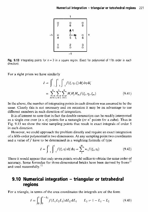
Fig. 9.13 Integrating points for n = 3 in a square region. (Exact for polynomial of fifth order in each direction).

For a right prism we have similarly

n n n

(9.41)

In the above, the number of integrating points in each direction was assumed to be the same. Clearly this is not necessary and on occasion it may be an advantage to use different numbers in each direction of integration.

It is of interest to note that in fact the double summation can be readily interpreted as a single one over (n x n) points for a rectangle (or n3 points for a cube). Thus in Fig. 9.13 we show the nine sampling points that result in exact integrals of order 5 in each direction.

However, we could approach the problem directly and require an exact integration of a fifth-order polynomial in two dimensions. At any sampling point two coordinates and a value off have to be determined in a weighting formula of type

(9.42)

There it would appear that only seven points would suffice to obtain the same order of accuracy. Some formulae for three-dimensional bricks have been derived by Irons' and used successfully.'2

9.1 0 Numerical integration - triangular or tetrahedral regions

For a triangle, in terms of the area coordinates the integrals are of the form 1 I L L . ,

I = jo Io f (Ll L2L3) dLz dL1 L3 = 1 - L1 - L2 (9.43)


Table 9.2 Numerical integration formulae for triangles

Order Figure Triangular

Error Points coordinates Weights

a 1 1 0 - I

0 1 1 I

C 1 0 1 -

2 1 2 ’ 3

R = 0 ( h 3 ) b 1 2 ’ 2 3 I 3 2 ’ ’ 2

Quadratic

a R = 0 ( h 4 ) b 0.6,0.2,0.2

C 0.2,0.6,0.2 d 0.2,0.2,0.6

21 1 1 1 _ _ 3 ’ 3 ’ 3 48

Cubic

Quintic R = 0 ( h 6 )

a 1 1 1 3 ’ 3 ’ 3

C

b f f l r P I 9 P I

PI > C Y I , PI d PI>Pl,ffl e f f 2 , P 2 , P 2

f P 2 , f f 2 , P 2

g P 2 , P 2 , 0 2

0.225 000 000 0

0.132394 1527

0.125 939 180 5

with CYI 0.059 715 871 7 PI = 0.470 142 064 1

0.797 426 985 3 P 2 =0.1012865073

Once again we could use n Gauss points and arrive at a summation expression of the type used in the previous section. However, the limits of integration now involve the variable itself and it is convenient to use alternative sampling points for the second integration by use of a special Gauss expression for integrals of the type given by Eq. (9.37) in which w is a linear function. These have been devised by Radau13 and used successfully in the finite element context.14 It is, however, much more desirable (and aesthetically pleasing) to use special formulae in which no bias is given to any of the natural coordinates Li. Such formulae were first derived by Hammer et ~ 1 . ’ ~ and Felippa16 and a series of necessary sampling points and weights is given in Table 9.2.17 (A more comprehensive list of higher formulae derived by Cowper is given on p. 184 of reference 17.)

A similar extension for tetrahedra can obviously be made. Table 9.3 presents some formulae based on reference 15.

Required order of numerical integration 223

Table 9.3 Numerical integration formulae for tetrahedra

No. Order Figure Tetrahedral

Error Points coordinates Weights

2 Quadratic R = o(h3)

C Y , P, P> P P, a, P, P P, P, a, P P, P, P, a CY = 0.58541020 P = 0.138 19660

I 4

4 5

_ _

l l l l 6 ’ 2 ’ 6 ’ 6 - 1 1 1 1 20 6 1 6 ’ 2 ’ 6

6 ’ 6 ’ 6 ’ 2

9 3 Cubic R = 0(h4) _ _ - - - _ _ - - e 1 1 1 1

9.1 1 Required order of numerical integration With numerical integration used in place of exact integration, an additional error is introduced into the calculation and the first impression is that this should be reduced as much as possible. Clearly the cost of numerical integration can be quite significant, and indeed in some early programs numerical formulation of element characteristics used a comparable amount of computer time as in the subsequent solution of the equations. It is of interest, therefore, to determine (a) the minimum integration requirement permitting convergence and (b) the integration requirements necessary to preserve the rate of convergence which would result if exact integation were used.

It will be found later (Chapters 10 and 12) that it is in fact often a positive disadvantage to use higher orders of integration than those actually needed under (b) as, for very good reasons, a ‘cancellation of errors’ due to discretization and due to inexact integration can occur.

9.11.1 Minimum order of integration for convergence

In problems where the energy functional (or equivalent Galerkin integral statements) defines the approximation we have already stated that convergence can occur providing any arbitrary constant value of the mth derivatives can be reproduced.

mapped elements and numerical 'singularity' …freeit.free.fr/finite...

Documents