marchi, tommaso - michigan state university
TRANSCRIPT
Università degli Studi di Padova
Dipartimento di Fisica
SCUOLA DI DOTTORATO DI RICERCA IN FISICA
CICLO XXV
Nuclear structure evolution far from stability:
study of 74Ni collectivity by Coulomb excitation
Direttore della Scuola: Ch.mo Prof. Andrea Vitturi
Supervisori: Prof.ssa G. Montagnoli
Dott.ssa F. Gramegna
Dott. G. De Angelis
Dottorando: Tommaso Marchi


Abstract
In recent years, the availability of neutron-rich radioactive ion beams has allowedto explore new regions of the nuclear chart. Despite the most exotic nuclei havebeen produced with quite low intensities, new interesting results have revealed anevolution of the nuclear structure far from the valley of β stability. Some of the wellestablished fundamental properties of the nuclear models, like the magic numbers,had to be reviewed in the light of new experimental observations: new features havebeen included in nuclear models in order to reproduce experimental data. It wasrecently shown, indeed, that tensor and three-body forces play an important role inbreaking and creating magic numbers.One region of particular interest is the neutron-rich tail of the Ni isotopic chain. Forinstance, the 78Ni nucleus corresponds to a double shell closure and is characterized bya large neutron excess. Some models predict that at this N/Z ratio one could expectan increase of the proton-neutron interaction strength that would modify the relativeenergies of the single particle states, thus reducing the Z = 28 energy gap. In such ascenario, particle-hole excitations should be strongly increased, driving to enhancedcollectivity. The determination of the B(E2) values of the low-lying transitions istherefore very important to measure these features and to constrain the interactionused for the shell model calculations.In this thesis we present the measurement of the B(E2; 0+ → 2+) transition matrixelement for the first 2+ state of the 74Ni nucleus.This was done in an intermediate-energy Coulomb excitation experiment performedat NSCL (MSU) where the Coulomb excitation cross section σ0+→2+ was measured,allowing to extract the B(E2 ↑) value. To date, 74Ni is the most exotic Ni isotopeproduced with enough intensity to be used as a beam for spectroscopic studies. The74Ni beam has been produced by fragmentation of a primary 86Kr beam at 140 AMeV

ii
on a 9Be target. The primary beam was provided by the Coupled Cyclotron Facilityof the NSCL and the produced reaction fragments were analyzed using the A1900fragment separator. As a matter of fact, this setup produced a secondary ”cocktail-beam“ containing 74Ni ions with an intensity of ≈ 1 pps as well as higher intensity 77Znand 75Cu fragments. A 197Au foil was used as secondary target. The scattered ionswere identified by the focal plane detectors of the S800 spectrograph and coincidenceγ-rays emitted by Coulomb excited ions were detected by the 4π CAESAR array.The results emerging from the data analysis show a different behavior with respectto the expectations. This finding opens new scenarios in the interpretation of theshell evolution of the Z=28 isotopes.The thesis has been organized as follows: the basic concepts concerning NuclearStructure studies far from stability and the radioactive ion beams production areintroduced in chapter 1. In chapter 2 the fundamental theoretical models of Coulombexcitation are presented. In chapters 3 and 4 the experimental setup and the dataanalysis of the Coulomb excitation experiment are respectively described. The finalresults are discussed in the last section. Considerations on possible interpretation ofthe Ni shell evolution will be presented together with some outlooks.

Riassunto
Negli ultimi anni, lo sviluppo di infrastrutture per la produzione di fasci di nucleiinstabili (radioattivi) ha permesso di esplorare nuove regioni della carta dei nuclidi,lontano dalla valle di stabilità. Nonostante le tecnologie attuali non permettano diprodurre fasci esotici di intensità paragonabili a quelle dei fasci stabili, varie in-formazioni sulla struttura nucleare lontano dalla valle di stabilità sono già stateottenute. Si è osservato, ad esempio, che proprietà ben assodate, come la chiusuradi shell in corrispondenza di determinati numeri magici e l’ordinamento delle shellprevisto dai modelli tradizionali, non sono più valide in presenza di una forte asim-metria di isospin. La formazione di aloni neutronici e la comparsa di nuovi numerimagici a discapito di quelli tradizionali sono due esempi del nuovo panorama che staemergendo. Quando ci si allontana dalle regioni per le quali sono stati sviluppati edottimizzati, i modelli tradizionali non riescono più a descrivere in maniera appropri-ata la struttura nucleare. In questo contesto, si rendono necessari termini correttivitra i quali le interazioni di tipo tensoriale e le forze a tre corpi si sono dimostrate diparticolare efficacia.Una regione interessante è rappresentata dalla parte ricca di neutroni della catenaisotopica del Nichel, in particolare nelle vicinanze del 78Ni. Secondo lo sviluppotradizionale delle shell nucleari, questo nucleo presenta una doppia chiusura di shell(Z = 28, N = 50). Tuttavia, alcuni nuovi modelli prevedono che con questo rap-porto N/Z ci si debba attendere un incremento dell’interazione neutrone-protonetale da modificare le energie relative dei livelli di particella singola, riducendo il gapdella shell protonica. In questa situazione, le eccitazioni particella-buco dovrebberoessere maggiormente favorite e presentare un comportamento fortemente collettivo.L’andamento degli elementi di matrice ridotti (B(E2)) delle transizioni dei livelli ec-citati più bassi di questi nuclei rappresenta uno degli indicatori più importanti per

iv
validare le ipotesi fatte e fornire informazioni quantitative per lo sviluppo di modellinucleari appropriati.In questo lavoro di tesi verrà descritto l’esperimento per la misura della B(E2; 0+ →2+) del primo livello eccitato (2+) del nucleo 74Ni tramite la misura della sezioned’urto di eccitazione coulombiana ad energie intermedie. Tale nucleo risulta, ad oggi,l’isotopo del Nichel più esotico ad essere stato prodotto con intensità di fascio suf-ficienti da consentire studi di tipo spettroscopico. L’esperimento è stato realizzatopresso il National Superconducting Cyclotron Laboratory (NSCL) della Michigan StateUniversity. Il fascio di 74Ni è stato prodotto per frammentazione di un fascio pri-mario (stabile) di 86Kr accelerato dalla Coupled Cyclotron Facility ad un’energia di140 AMeV e diretto su un bersaglio di 9Be. Quì, principalmente in seguito a reazionidi frammentazione del proiettile, sono state prodotte numerose specie nucleari. Laselezione degli isotopi di interesse, realizzata dal separatore elettromagnetico A1900,ha consentito di isolare un fascio secondario (”cocktail-beam“) contenente ioni di74Ni con un’intensità di circa 1 pps assieme ai più intensi fasci di 77Zn e 75Cu. Perl’eccitazione coulombiana è stato usato un foglio di 197Au spesso 640 mg/cm2. Gliioni in uscita dal bersaglio secondario sono stati identificati dai rivelatori di pianofocale dello spettrometro S800 ed i fotoni di diseccitazione emessi in coincidenza sonostati misurati utilizzando il rivelatore a 4π CAESAR.Dall’analisi dei dati realizzata in questo lavoro è emerso che, entro gli errori spe-rimentali, il valore della B(E2) è diverso da quanto osservato precedentemente uti-lizzando tecniche differenti. Questo risultato potrebbe pertanto aprire la strada anuove interpretazioni sull’evoluzione delle shell all’interno della catena isotopica delNi. Questo elaborato è organizzato nel modo seguente: nel primo capitolo verrannointrodotti i concetti principali riguardanti lo studio della struttura nucleare lontanodalla valle di stabilità e la produzione di fasci radioattivi. Nel capitolo 2 verranoillustrati gli aspetti fondamentali della teoria dell’eccitazione coulombiana in diversiregimi energetici. I capitoli 3 e 4 saranno dedicati, rispettivamente, alla descrizionedell’apparato e dell’analisi dei dati. I risultati ottenuti verranno infine commen-tati nell’ultima sezione. Verranno quindi discusse alcune possibili interpretazionisull’evoluzione della struttura nucleare nella catena isotopica del Nichel e presentatele prospettive sperimentali necessarie per una migliore comprensione della tematicadiscussa.

Contents
Abstract iii
Riassunto v
1 Nuclear Structure studies with radioactive ion beams 11.1 The Nuclear Chart, a wide landscape . . . . . . . . . . . . . . . . . . 21.2 Radioactive ion beam facilities . . . . . . . . . . . . . . . . . . . . . . 181.3 The Ni isotopic chain . . . . . . . . . . . . . . . . . . . . . . . . . . . 251.4 The experiment on 74Ni . . . . . . . . . . . . . . . . . . . . . . . . . 30
2 Coulomb Excitation 332.1 Gamma Decay . . . . . . . . . . . . . . . . . . . . . . . . . . . . . . . 342.2 Elastic Coulomb Scattering . . . . . . . . . . . . . . . . . . . . . . . 372.3 Theory of Coulomb Excitation . . . . . . . . . . . . . . . . . . . . . . 382.4 Accuracy of Coulomb excitation at intermediate energies . . . . . . . 492.5 Cross sections calculation . . . . . . . . . . . . . . . . . . . . . . . . 50
3 Experimental setup 533.1 Primary beam production and acceleration . . . . . . . . . . . . . . . 543.2 Primary target . . . . . . . . . . . . . . . . . . . . . . . . . . . . . . 553.3 A1900 Fragment Separator . . . . . . . . . . . . . . . . . . . . . . . . 563.4 S800 spectrometer . . . . . . . . . . . . . . . . . . . . . . . . . . . . 593.5 S800 Focal Plane Detectors . . . . . . . . . . . . . . . . . . . . . . . 613.6 CAESAR array . . . . . . . . . . . . . . . . . . . . . . . . . . . . . . 66

vi CONTENTS
4 Data Analysis 774.1 Focal plane detectors calibration . . . . . . . . . . . . . . . . . . . . . 784.2 CAESAR calibration . . . . . . . . . . . . . . . . . . . . . . . . . . . 824.3 GEANT4 simulation . . . . . . . . . . . . . . . . . . . . . . . . . . . 864.4 Detection Efficiency . . . . . . . . . . . . . . . . . . . . . . . . . . . . 884.5 Particle Identification . . . . . . . . . . . . . . . . . . . . . . . . . . . 914.6 Event selection . . . . . . . . . . . . . . . . . . . . . . . . . . . . . . 994.7 Excitation Cross Section . . . . . . . . . . . . . . . . . . . . . . . . . 105
5 Results and conclusion 111
References 124

1Nuclear Structure studies with radioactive
ion beams
The development of new instrumentation and acceleration techniques has alwaysbeen crucial for nuclear structure studies. Whenever new experimental tools foraccelerating and detecting particles and nuclear radiation have been developed, newand quite often unexpected features have shown up.In particular, the development of techniques to produce and accelerate unstable nuclei(the so-called Radioactive Ion Beams) opens up new possibilities to access and studynuclei with large neutron excess (neutron-rich nuclei). This is one of the “hot”topics of contemporary Nuclear Structure studies because it allows to explore regionsof the nuclear chart that are not commonly accessible. Beyond the possibility ofdiscovering new isotopes, researchers have the opportunity to test the validity ofnuclear structure and nuclear reaction models while moving far from the conditionswhere they have been developed and tested. New scenarios arose in recent yearsthanks to the availability of radioactive beams with increasing neutron/proton ratio.For instance, the rearrangement of the nuclear shells and the related appearance of

2 1. Nuclear Structure studies with radioactive ion beams
new magic numbers shows that the global features of the nuclear force change whileincreasing the number of neutrons in the nuclear system.In this chapter, some of the current topics in Nuclear Structure will be reviewed. Wewill describe how the availability of radioactive ion beams allows to probe the behaviorof nuclear shells far from the stability line and which are the current limits in thestudy of very neutron-rich nuclei. Particular care will be put on the structure of theNi isotopic chain. The nuclear shell evolution in the region close to the doubly magic78Ni will be described in order to better understand the relevance of the measurementof the reduced matrix element B(E2 ↑) of the 74Ni isotope, which is the main subjectof the present Thesis.
1.1 The Nuclear Chart, a wide landscape
“Atomic nuclei comprise 99.9% of all baryonic matter in the Universe and arethe fuel that burns in stars. The rather complex nature of the nuclear forces amongprotons and neutrons generates a broad range and diversity in the nuclear phenomenathat can be observed” [1]. The atomic nucleus is indeed a quantum-mechanical systemwhere a number of Z protons and of N neutrons (the nucleons) are held bound bythe strong force. The proton carries electric charge while the neutron does not. Forthis reason, protons in nuclei also feel their mutual Coulomb repulsion. To obtain abound system the two forces have to counterbalance. The net result is a system witha degree of complexity that increases with the number of nucleons A = N + Z (i.e.the nuclear mass). There are many combinations of neutrons and protons which canform a nucleus of a given mass. The wide landscape of nuclei offered by Nature isusually summarized in the so-called Nuclear Chart shown in figure 1.1.
To date, around 3000 nuclei have been observed. About 250 nuclides, correspond-ing to the black squares of figure 1.1, are stable and can be found naturally. Theremaining observed nuclei, corresponding to the yellow boxes of figure 1.1, are unsta-ble and they ultimately convert to a stable isotope via a chain of radioactive decays,the lifetimes of which might range from nanoseconds to millions of years. Most ofthe observed unstable nuclei have been artificially produced in a laboratory, thoughsome of them can be found in Nature as part of the decay chain of extremely long-lived isotopes. Theoretical models predict the existence of more than 6000 nuclear

1.1 The Nuclear Chart, a wide landscape 3
Figure 1.1: Nuclear Chart. Colors are used to group nuclei according to the type of de-cay. Black dots represent stable nuclei accumulating along the valley of nuclear stability.The yellow area corresponds to experimentally observed unstable isotopes while the greenarea shows unstable nuclei which are predicted to be bound but which have not yet beenobserved. Adapted from [2].
bound systems (the green squares of figure 1.1), meaning that only half of the globalpanorama has been explored to date.More generally speaking, the limits of nuclear stability provide a key benchmark ofnuclear models. These limits also highlight the emergence of new phenomena leadingto extra binding and to an extension of the expected limits of stability, as it has beendiscovered for halo nuclei [3]. The boundary limits for extremely neutron-deficientnuclei and the location of the proton drip-line are fairly well defined, but very littleis known about the limits of binding of very neutron-rich nuclei and the location ofthe neutron drip-line, which are established experimentally only for the eight lightestelements [4]. The neutron deficient part of the nuclear chart can be accessed ex-perimentally using fusion evaporation reactions. On the contrary, in order to studythe neutron-rich side of the nuclear chart, new tools should be developed such asthe production of beams of (unstable) neutron-rich nuclides, namely the radioactiveion beams. Those beams will provide experimental access to the nuclear properties

4 1. Nuclear Structure studies with radioactive ion beams
of heavy neutron-rich nuclei that will drive the development of nuclear models withgreatly improved predictive power. Indeed, there is a broad agreement in the nuclear-science community that the critical path to improvements in nuclear modeling passesthrough neutron-rich nuclei far from the line of β-stability. Their properties mustbe known to determine the actual degrees of freedom and to constrain the effectiveinteractions such as the tensor force [5], the symmetry energy [6], and the isospindependent three-body forces [7] which are, so far, only poorly determined.From the theoretical point of view, even assuming a very simple parametrization ofthe nuclear potential, the solution of the quantum-mechanical many body problembecomes almost impossible already at very low mass numbers. Modern ab-initio cal-culations use a realistic expression of the nucleon nucleon interaction to calculatenuclear properties in computational frameworks like Green’s function Monte Carlo,no-core shell model or coupled cluster method. They are successful when the nuclearmass is small (i.e. up to A = 8 or so) but, when the number of nucleons increases,computational times diverge. For this reason, several macroscopic approaches areused for medium-mass or heavier nuclei where the great success of the shell modelis evident. In this field, modern configuration interaction techniques are used. Forvery heavy nuclei, the density functional theory based on self-consistent/mean fieldapproaches is the tool of choice. By investigating the intersections between these the-oretical strategies, theorists aims at developing a unified description of the nucleus.Figure 1.2 shows how theoretical models match the nuclear chart and how differentapproaches overlap in boundary regions.In this work we will focus on the neutron-rich side of the Ni isotopic chain, that isstudied in detail from the theoretical point of view using mean field and shell modelcalculations. We will introduce in the next paragraph some interesting phenomenathat arise while moving far from the stability line, increasing the number of neutronsin the nucleus.
1.1.1 Nuclear shells far from stability
Ideally, as mentioned in section 1.1, one could think of deriving the nuclear proper-ties starting from a more or less detailed knowledge of the nucleon-nucleon interaction(the so-called ab-initio approach). As already mentioned in the previous paragraph,the solution of the quantum-mechanical many body problem becomes almost impos-

1.1 The Nuclear Chart, a wide landscape 5
Figure 1.2: Theoretical approaches used in the various regions of the chart of nuclides.In the low-mass region ab-initio calculations are possible. Moving to higher masses, ex-tended shell model approaches (here stated as configuration interaction) are widely ex-ploited. For the heaviest part of the diagram only mean field calculations can be used(i.e. density functional theories). Adapted from [8].
sible already at very low mass numbers. For larger masses, presently up to A ≈ 80,the complementary approach of the Nuclear Shell Model is highly successful. TheNuclear Shell Model is indeed one of the earliest models developed to describe theproperties of the known nuclides and, incidentally, it is one of the most successfulmodels developed so far. It relies ultimately on the concept of single-particle motionin an average mean field. This can be explained considering the nuclear hamiltonian:
H =A∑i=1
[p2i
2 mi
]+
A∑i,k
Vik(ri − rk). (1.1)
Here A is the number of nucleons, the first term is their kinetic energy and thesecond one is the two-body interaction potential. For the moment, third or higherorders interaction terms are neglected. In the mean-field hypothesis, one assumesthe existence of a single-particle potential V (r) that absorbs most of the Vik(ri − rk)

6 1. Nuclear Structure studies with radioactive ion beams
potential. In other words, one assumes that each nucleon moves independently fromthe others in a potential generated by the other nucleons themselves. This results inthe separation of the hamiltonian in two components:
Hi =∑A
i=1
[p2i
2 mi
]+∑A
i=1 Vi. (1.2)
Hresi,k =
∑Ai,k Vik −
∑Ai=1 Vi. (1.3)
where
H = Hi +Hresi,k . (1.4)
The Hi part is the one describing the motion of the nucleon in the nucleus (alsocalled the single-particle hamiltonian), while Hres
i,k is the residual interaction betweennucleons that is not considered by the mean-field. This component has to be smallcompared to the single-particle one. Under these assumptions, a shell structure,similar to the atomic shell structure, appears in a quite natural way. The meanpotential can be described, to a good approximation, in terms of the so called Woods-Saxon potential. This is specified by the parameters depth (V0), radius (R0) anddiffuseness (a):
V (r) = − V0
1 + exp r−R0
a
. (1.5)
The eigenstates of this potential can be obtained only numerically, thus the Har-monic Oscillator potential is often used as a convenient approximation since it canbe treated analytically. The expression of this potential is:
Vi =1
2miω
2r2i (1.6)
where mi is the mass of the ith nucleon, ω is the oscillator frequency and r stands forthe distance from the center of the nucleus. As shown in the left part of figure 1.3, theeigenvalues of the harmonic oscillator corresponding to the principal quantum numberN are evenly spaced in energy. In this simple model the sub-levels corresponding todifferent values of the angular momentum l are degenerate. Thus one can identifygroups of levels (shells) with “large” separation between the groups. The filling of

1.1 The Nuclear Chart, a wide landscape 7
all the sub-levels corresponding to a given value of N , in other words, the filling of amajor shell, should correspond to particularly stable nuclei.
Figure 1.3: Energy eigenvalues of the harmonic oscillator with and without the spin-orbit splitting. The right panel shows the magic numbers introduced by Mayer andJensen. Adapted from [9].
This explains why some nuclides, namely the magic or doubly-magic nuclei, areparticularly stable as pointed out by the early experimental findings. With this simplemodel, only the lowest magic numbers (up to Z,N=20) are reproduced. In order toreproduce all of the observed magic numbers, it is necessary to take a further spin-orbit term into account, describing the interaction between the spin of the nucleonand its orbital angular momentum:
Vls(r) = f(r)(l · s) (1.7)
This was done in the independent works of Mayer [10] and Jensen [11] who addeda spin orbit coupling term to the Harmonic Oscillator potential, succeeding in the

8 1. Nuclear Structure studies with radioactive ion beams
interpretation of the experimental data available at that time. This calculation leadsto the splitting of the single particle levels that re-arrange in terms of energy as shownin figure 1.3.
From the above description, it should be clear that the location and size of shell gapsdepend on the specific details of the mean field and the residual interaction betweenthe valence nucleons considered. It is worth to underline that most of the nuclearmodels have been developed and tested with the available data about nuclei veryclose to stability. Therefore, the “traditional” magic numbers discovered for stablenuclei and the shell ordering should not be expected to remain the same throughoutthe whole chart of nuclides. The question of the shell evolution moving towardsthe neutron-rich regions is indeed one of the most actual topics of modern NuclearStructure. Extrapolating towards exotic nuclei the models developed and tested forthe isotopes near the stability line is a quite delicate question.
Figure 1.4: Scale-type ls quenching. In neutron-rich nuclei the spin-orbit force shouldbe weaker as a consequence of the diffuseness of nuclear surface. [12]

1.1 The Nuclear Chart, a wide landscape 9
Scale-type ls quenching
The availability of the very first generation of radioactive ion beams already trig-gered the development of many theoretical schemes, trying to explain some of thenewly observed features and to develop some more general frameworks. One of theseis the so-called scale-type ls quenching [13]. Since the spin-orbit force is proportionalto the radial derivative of the potential, its strength may be weakened with a diffusesurface region (see figure 1.4) where the neutron excess causes a softer decrease ofthe nuclear density (or neutron skin) [13]. Thus, the magic numbers identified nearstability could change for neutron-rich nuclei (fig. 1.5) revealing a more harmonic-oscillator like behavior. Some calculations indicate that, near the neutron drip line,one may encounter quenching of existing shell gaps leading to the emergence of newmagic numbers. It is clear that these effects have to be expected very close to theneutron drip-line, where the appearance of a neutron skin becomes an appreciablephenomenon. As it can be seen in the nuclear chart (fig. 1.1), the neutron drip-lineis experimentally accessible only for the lightest elements and it is increasingly farfrom the most exotic isotope observed as one moves towards heavier nuclei. For thisreason scale-type ls quenching cannot be considered the only reason of the observedevolution of the nuclear shells.
Figure 1.5: Possible evolution of the nuclear shells due to surface diffuseness movingtowards the neutron drip-line. Adapted from [14].

10 1. Nuclear Structure studies with radioactive ion beams
The tensor force
T. Otsuka and co-workers recently pointed out the importance of the tensor forcecomponent in the parametrization of the nuclear potential [15, 16]. As introduced byYukawa in 1938, the nucleon-nucleon interaction can be explained in terms of mesonexchange. In this framework, the π+ρ meson exchange term is essentially the tensorforce that can be parametrized in the mean field approach considering a potentialterm like [17]:
VT = (τ1 · τ2) S12 V (r) (1.8)
where τ1,2 denotes the isospin of the nucleons 1 and 2, V (r) is a function of therelative distance of the nucleons (r) and S12 (depending on s1 · s2, where τ1,2 is thespin of the nucleons) denotes the spin coupling, as explained with details in reference[18].
As shown in figure 1.6, this neutron-proton interaction has the effect to change thesingle particle energies as a function of the N/Z ratio. For instance, if j> = l+1/2 andj< = l−1/2, neutrons in j′> orbit lower the proton orbit with j< but raise the protonorbit j>. Using this parametrization, it was shown that this term affects the shellstructure in a robust way when considering exotic nuclei. A schematic overview of thepossible effects was obtained in the work of Otsuka and collaboratros [5], which wasfocused on the evolution of the proton and neutron single particle energies calculatedadding the tensor term into a Gogny-type mean field calculation (called GT2). Morerecently [16] the results obtained by successful shell-model effective interactions likeGXPF1 [19] have been compared to what can be described using the tensor forceadded to a Gaussian central potential. Given the good agreement with the existingtheories, the monopole based universal interaction (VMU) was introduced. As shownin figure 1.7 (left panel), this potential consists of two terms: the first term is aGaussian central force representing the bulk nuclear properties and re-normalized toexperimental observations, while the second one is due to the tensor force. Using thisparametrization, the shell evolution of neutron and proton single particle energieshas been studied. Some results for the Ni isotopic chain are shown in the right panelof figure 1.7.

1.1 The Nuclear Chart, a wide landscape 11
Figure 1.6: Panel (a) is a schematic picture of the monopole interaction produced bythe tensor force between a proton in j>,< = l ± 1/2 and a neutron in j′>,< = l′ ± 1/2.Panel (b) shows the exchange processes contributing to the monopole interaction of thetensor force. Adapted from [17].
π + ρ meson
(b) tensor force(a) central force
V =MU+
exchange
-20
-10p1/2
f 7/2
f 5/2
p3/2
ε(M
eV
)
40 50N
Z=28, proton SPE
Figure 1.7: Left panel. Diagrams for the VMU interaction. a) Central force compre-hensive of experimental renormalization. b) Tensor force term (the same as 1.6 b). Rightpanel. Single particle energies for the Ni isotopes as calculated by VMU . The attractionbetween f7/2 and f5/2 causes the inversion of the p3/2 and of the f5/2 orbitals. Adaptedfrom [16].

12 1. Nuclear Structure studies with radioactive ion beams
Three body forces
Another topic under discussion, needed to explain the properties of the nuclearpotential far from stability, is the inclusion of three-body forces. For instance, thesemechanisms are used to explain the behavior of the neutron drip-line in regions wherestandard shell-model calculations fail. This is the case of the Oxygen isotopes re-ported in [20], where experimental observations underlined that the neutron drip-lineof oxygen is closer to the stability line as compared to the basic trend. Moreover,adding only one proton (the fluorine case), the drip-line is back to the trend. Oxygenisotopes can be described as a multi-neutron system on top of the closed-shell 16Ocore. The experimental ground-state energies are shown in figure 1.8. One can cal-culate the interaction between these valence neutrons in the sd shell by microscopicmethods. Some examples are are shown in figure 1.8. One finds that, without theinclusion of three-body terms, the ground-state energy keeps going down all the wayto N = 20. This contradicts the experimental fact that the drip-line is at N = 16.The problem is overcome by considering the repulsive contributions to the interactionamong excess neutrons, namely the three-body interaction.The importance of this mechanism is also evidenced in the work of Hagen and collabo-rators [21] who succeeded in performing approximate ab-initio calculations employinginteractions from chiral effective field theory. The binding energies and low-lying ex-citations of Calcium isotopes have been computed using the coupled-cluster methodand it was shown (figure 1.9) that the phenomenological inclusion of three body forcesplays an essential role when comparing to experimental data.
1.1.2 Experimental probes
Some consequences of these theoretical predictions on the shell evolution have beenpointed out. A change in the magic numbers is expected [22] (see figure 1.10) andindeed new ones have been discovered in the recent years (e.g. N = 16, N = 32)whereas well established ones might disappear (e.g. N = 20, Z = 14). In looking fornew (sub)shell closures the most sensitive and direct signature can be derived from

1.1 The Nuclear Chart, a wide landscape 13
−60
−40
−20
0
8 16 2014Neutron Number (N)
Ene
rgy
(MeV
)(a) Energies calculated from phenomenological forces
SDPF-MUSD-B
Exp. Exp.
(b) Energies calculated from G-matrix NN
+ 3N (Δ) forces
(c) Energies calculated from V NN
+ 3N (Δ,N LO) forceslow k
2
NN
NN + 3N (N LO) NN + 3N (Δ)
Exp.2 O core16
(d) Schematic picture of two- valence-neutron interaction induced from 3N force
NNNN + 3N (Δ)
8 16 2014Neutron Number (N)
8 16 2014Neutron Number (N)
−60
−40
−20
0
Ene
rgy
(MeV
)
Figure 1.8: Experimental ground-state energies of the Oxygen isotopes measured from16O, including experimental values of the bound 16−24O compared to energies obtainedfrom (a) phenomenological forces, (b) a G matrix formalism including three body forces,(c) low-momentum interactions Vlow k and including three body forces. (d) Schematicillustration of a two-valence-neutron interaction generated by three body forces with anucleon in the 16O core. Figure adapted from [20], see reference for details.
binding energies. The second differences:
δ2n(Z,N) = S2n(Z,N + 2)− S2n(Z,N)
δ2p(Z,N) = S2p(Z + 2, N)− S2p(Z,N) (1.9)

14 1. Nuclear Structure studies with radioactive ion beams
39 40 41 42 47 48 49 50 51 52 53 54 55 56 59 60 61 62A
-500
-480
-460
-440
-420
-400
-380
-360
-340
-320
E (M
eV)
NN + 3NFeffExperimentNN only
Figure 1.9: Ground-state energy of the Calcium isotopes as a function of the mass num-ber A as calculated using the coupled cluster method. Black circles: experimental data;red squares: theoretical results including the effects of three-nucleon forces; blue dia-monds: predictions from chiral NN forces alone. Figure adapted from [21].
where
S2n(Z,N) = BE(Z,N)−BE(Z,N − 2)
S2p(Z,N) = BE(Z,N)−BE(Z − 2, N) (1.10)
show a distinct peak for closed-shell nuclei and its height represents the shell gap.However, a basic change of the underlying nuclear structure, as, e.g., quadrupolecorrelations, can severely distort δ, since the binding energies of three nuclei areinvolved in equation 1.9. Similar indications about the underlying shell structure aregiven by the one-nucleon (proton or neutron) separation energies or by the differencebetween the same value in two consecutive nuclei as shown in figure 1.11.
More indirect measures for shell closures are the excitation energies of the firstexcited 2+ states, E(2+) and the reduced transition strength, B(E2;2+ → 0+). Theparticular stability of magic and doubly magic nuclei is expected to result in highexcitation values for the first excited state (E(2+)). Concerning the B(E2) values,transitions in nuclei a few particles apart from a shell closure are mostly due tothe contribution of a single particle, therefore these nuclei are expected to have low

1.1 The Nuclear Chart, a wide landscape 15
Figure 1.10: Schematic chart of known and expected new shell structure in N ≫ Znuclei. Known and new closed shell nuclei are indicated respectively as full and hatchedsquares [22].
reduced transition probabilities, close to the single particle estimate (see 2.1). Inthe opposite situation, at mid-shell, several particles can contribute coherently to thetransition, resulting in high B(E2) values. This is what is typically described as a”collective“ behavior. For instance, in figures 1.12 and 1.13 [24, 25] the δ2n/2p, B(E2)(in Weisskopf units) and E(2+) are shown for the closed shells Z = 8, Z = 20 andZ = 28. To demonstrate the isospin symmetry and to integrate the scarce data, themirror nuclei with N = 8, 20, 28 are overlapped. The known magic nuclei, such as16O and 40Ca, clearly stand out in these plots, and evidence for semimagicity of others,e.g. 34Si, can be found. In recent years these studies have been pursued in severalfacilities, both using stable and unstable beams. For instance, one such campaign

16 1. Nuclear Structure studies with radioactive ion beams
diff
ere
nce
s o
f S
_n
(M
eV
)
N
0
2
4
6
8
0 50 100 150
S_
n (
Me
V)
0
5
10
15
Figure 1.11: Top panel: one-neutron separation energies as a function of neutron num-ber for even-even nuclei with N > Z. The lines connect nuclei with the same Z value.Bottom panel: difference between one-neutron separation energy for the same set ofeven-even nuclei. The dashed lines show the magic numbers 8, 20, 28, 50, 82 and 126.Adapted from [23].
of experiments has been carried out at the Laboratori Nazionali di Legnaro usingthe CLARA array of Clover detectors [26] in coupled operation with the PRISMA

1.1 The Nuclear Chart, a wide landscape 17
Figure 1.12: Shell signatures δ2n/2p, B(E2;2+ → 0+) and E(2+) for shell evolution ofnuclei (a) Z = 8 oxygen isotopes (full-line) and N = 8 isotones (dashed); (b) Z = 20calcium isotopes (full-line) and N = 20 isotones (dashed). [24]
Figure 1.13: Shell signatures δ2n/2p, B(E2;2+ → 0+) and E(2+) for shell evolution ofnuclei Z = 28 nickel isotopes (full-line) and N = 28 isotones (dashed). [25]
magnetic spectrometer [27]. A similar campaign of measurements has been latercarried out using the AGATA Demonstrator Array [28] coupled to the PRISMAspectrometer. Even if a lot of work has been done, only the use of highly exoticprojectiles will allow to explore the extreme limits of the nuclear chart. Therefore it

18 1. Nuclear Structure studies with radioactive ion beams
is clear to the Nuclear Physics community that the future developments in this fieldof research will strongly depend on the availability of intense radioactive ion beamsproduced in dedicated facilities.
1.2 Radioactive ion beam facilities
Studies have been carried out in the last decade at the first generation radioactiveion beam (RIB) facilities. A brief summary of the working principles of a RIB facilitywill be given, together with a description aimed at explaining what is expected toupgrade their technical properties in the near future.There are two different methods for the production of a radioactive ion beam: theIsotope Separation On-Line (ISOL) and the In-Flight technique (IF). Both have ad-vantages and disadvantages and can be somehow considered complementary.The ISOL method is the oldest one and can be attributed to the pioneering workof O.Kofoed-Hansen and K.O.Nielsen in 1951. Their technique consisted in bom-barding an Uranium target with fast neutrons coming from the break-up of a 11MeV deuteron beam. Neutron-rich, noble gas isotopes produced through fission wereswept into the ion source of an electromagnetic isotope separator after thermalizationin the target. The whole process of production, ionization, mass-separation, implan-tation into a detector set-up and subsequent detection of the emitted decay radiationwas performed in a continuous way, hence the name: “Isotope Separation On Line”.The ISOL method, schematically drawn in figure 1.14, is based on the production ofradioactive species by spallation, fission or other nuclear reactions in a thick targetat rest. These reactions can be induced by neutrons or photons as well as by intensebeams of charged particles. Neutrons are available as a by product of nuclear reactorsor can be produced by a converter. High fluxes of photons can be obtained by thebremsstrahlung of intense energetic electron beams impinging on Tungsten targets.The more straightforward approach to directly use an intense beam of charged parti-cles on a thick target has the drawback of the heat load of the target itself, which canlimit the power on target that can be dissipated. This problem has been studied indetail and interesting solutions have been proposed [29, 30]. The isotopes producedin the thick target are then extracted and ionized to a certain charge state in anion source. However, the diffusion in the target material depends on the chemical

1.2 Radioactive ion beam facilities 19
Figure 1.14: Schematic view of the ISOL technique. The high intensity primary beamimpinges on a thick target at high temperature. The reaction products are then extractedand ionized to produce the radioactive beam. This beam is then post-accelerated andused in nuclear physics experiments. Figure adapted from [14].
properties of the reaction products and may be quite long (of the order of seconds).Moreover, the effusion and ionization are also quite slow processes characterized bytimes up to several ms. The total process can be quite longer than the lifetime ofthe shortest lived isotopes. This means that there is an a-priori limit in the regionof the nuclear chart accessible with this technique. After the extraction from thetarget, the selected elements have to be ionized for a later magnetic separation andpre-acceleration. Depending on the requirements, several different ionization sourcesare used. For the RIB production, the source must operate steadily for extendedperiods of time at high temperatures (up to 2000C). The selection of the target/ion-source system is very important since it determines the intensity, beam quality andnumber of RIBs that can be provided for the experiment. The worldwide spread RIBfacilities make use of a large variety of solutions. Among the ion sources: surfaceionization (SIS), plasma (FEBIAD), electron cyclotron resonance (ECR) and reso-nant laser ion (RILIS) techniques are used. The first mechanism is based on surfaceionization: when an atom interacts with a heated surface, it can lose or gain oneelectron before leaving the surface. This technique is used for elements with verylow ionization potentials to generate positive and negative ions, respectively. The

20 1. Nuclear Structure studies with radioactive ion beams
surface ionization method is extremely selective when the elements produced in thesame reactions present different ionization potentials. The plasma ion source is basedon the Forced Electron Beam Induced Arc Discharge. It exploits the capabilities ofthe electrons produced from an indirectly heated disc-shaped cathode and acceler-ated into an anodic chamber, to ionize any atom entering the chamber volume whichhave an ionization potential smaller than the incident electron energy. It is workingproperly in conjunction with high temperature target material in a pressure rangeof 10−4 − 10−5 torr. Electron Cyclotron Resonance (ECR) sources are used for iso-topes of elements with ionization potentials higher than 7 eV and for the creation ofmultiply-charged ions. The ions are bombarded by energetic electrons and lose one ormore of their outer electrons. This method is not very chemical selective, due to thenon-selective nature of the ionization process. The resonance ionization ion source isbased on the Laser ionization process: atoms are stepwise excited by laser photonsinjected in the extraction beam-line. This ionization process is usually done in two orthree steps exploiting the atomic structure of the species of interest. For this reason,it allows for a very efficient elemental selection. After the ions are created in the ionsource, they are extracted and accelerated in a DC electrical field. This energy isnecessary for the transport and injection into an analyzing magnet where a first massseparation occurs. Since the selection process ends with a beam of very low energy,a further post acceleration is usually needed. As a result of this process, the qualityof the secondary beam, in terms of energy and emittance, will be comparable to thatof a stable beam from an existing facility.Several ISOL facilities have been and are currently operating worldwide. Among themwe underline the following: ISOLDE [31] at CERN, ISAC at TRIUMF (Canada) [32],HRIBF at ORNL (USA) [33]. It should be remarked that new projects to build ISOLfacilities are available at GANIL (SPIRAL II) [34] and at the Laboratori Nazionalidi Legnaro (SPES) [35]. The SPIRAL II project is based on a double step systemwhere a 40 MeV deuteron beam impinges on a converter to produce neutrons. Thelatter are used to induce fission on a very thick UCx target aiming at the productionof 1013 − 1014 fissions per second. The Selective Production of Exotic Species (SPES)project is concentrating on the production of neutron-rich radioactive nuclei withmasses in the 80-160 range, by Uranium fission at a rate of 1013 fission/s. The protondriver is a cyclotron with variable energy (15-70 MeV) and a maximum current of 500µA. In this case the proton beam will directly impinge on a segmented UCx target

1.2 Radioactive ion beam facilities 21
Figure 1.15: Schematic view of the In-Flight technique. A primary beam of stableheavy ions is accelerated to intermediate or high energy and impinges on the productiontarget. Fragmentation reactions produce a wide variety of stable and unstable nuclearspecies among which a fragment separator is used to isolate the isotopes of interest. Theradioactive beam is then sent to the experimental station. The Figure adapted from [14].
[36]. The produced RIBs will be post-accelerated with a superconducting LINACup to energies of 11 AMeV for masses around 130. These energies allow to over-come the Coulomb repulsion between the radioactive beam and the target nuclei ina large variety of systems. This feature, together with the increased beam intensitieswill allow new experimental studies employing different reaction mechanisms, suchas multi-step Coulomb excitation, inelastic scattering, single and multiple nucleontransfers and fusion reactions.
In the In-Flight RIBs production method (see figure 1.15), a heavy-ion beam atvery high energy (of the order of 40–2000 AMeV) collides with a target, inducing withhigh probability projectile fragmentation. After the primary target area, a complexsystem, composed of electric and magnetic separators and degraders, selects the de-sired isotopes, which can be focused to the secondary target position for the studiesof interest. This technique is used, for instance, at the NSCL Laboratory of MSUwhere the experiment subject of this Thesis was performed.In principle the projectile fragmentation gives rise to a large distribution of ionslighter than the projectile itself but only those reasonably close to the primary beam

22 1. Nuclear Structure studies with radioactive ion beams
Figure 1.16: Overview of the Radioactive ion beams production methods. The interplaybetween the In-Flight and ISOL techniques is underlined.
will be produced with high enough cross sections. Therefore only these nuclei willbe useful as secondary beams to produce further reactions for spectroscopic studies.The other products may only be used for mass measurement purposes aiming atthe discovery of new isotopes [37]. One of the main features of this method is thatthe process is almost independent of the chemical properties, or the half-life of theisotopes of interest. The limitation of the half-life is only given by the flight timeof the ions through the separator, which is generally less than 1 µs. Even thoughthe particle identification of fast ions is relatively simple, the selection process usingfragment separators results however in a lower beam purity with respect to the ISOLtechnique.The existing In-Flight radioactive beam facilities in Europe at GANIL [38] and GSI

1.2 Radioactive ion beam facilities 23
[39], together with their counterparts at RIKEN[40], Japan, and MSU [41], USA,developed methods for extracting valuable nuclear-structure information from scat-tering experiments with intermediate-to-high energy secondary beams of unstablenuclei, although restricted to nuclear masses up to A = 80 and intensities up to105-107 pps, which should be compared with the 1011 pps of a stable beam. Greatimprovements came from their operation in the last decades. Among these: the dis-covery of new isotopes, the measurement of several nuclear masses and the study ofnuclear spectroscopy of neutron-rich nuclei. Due to the low beam intensities avail-able up to now, the nuclear structure information is typically obtained through directreactions such as single nucleon transfer or Coulomb excitation. Even in the mostfavorable cases it is extremely difficult, if not impossible, to identify high-spin stateswith these techniques. In particular, using γ-spectroscopy, it is very difficult to studyexcited levels lying above the first excited state. Therefore, an increase in beamintensities by several orders of magnitude is aimed for, involving a large number oftechnological challenges.In this framework the SPES and SPIRAL II projects are considered as a first step(second generation facilities) towards the road of new very performing third genera-tion facilities.For the future development of more intense radioactive ion beams, the possibility of
combining the two complementary methods has been investigated as a way of over-coming their separate limitations. A general scheme is shown in figure 1.16. Oneof the new approaches to the production of low-energy radioactive beams involvesthe stopping of fast radioactive beams produced In-Flight, using a large gas catcherwhere the ions are thermalized in high-purity helium and extracted as singly chargedions for post-acceleration. This removes the limitation present in the standard ISOLtechnique for species that are difficult to extract from the target/ion source assem-bly. This is the case of the Facility for Rare Isotope Beams (FRIB) [42], which is anext generation facility proposed in the USA. Here, a primary heavy-ion acceleratorcapable of delivering intense ion beams up to uranium at 400 AMeV will be used forfission and fragmentation reactions. The produced ions will be either used as fastradioactive ion beams or thermalized by a gas-catcher and re-accelerated up to 12AMeV.FAIR [43] is a further next generation in-flight facility to be constructed at GSI [44].

24 1. Nuclear Structure studies with radioactive ion beams
Figure 1.17: World map of the main radioactive ion beam facilities. Table 1.1 can beused as a legend.
In this facility, two synchrotron accelerators will deliver heavy ion beams up to 1.5AGeV for the production of exotic nuclei from fission and fragmentation reactions.The produced nuclei will be separated and identified using the Super-FRS magneticspectrometer.On the other hand, a combined ISOL/In-Flight method has been proposed. The ideais to obtain extremely neutron-rich nuclei from the fragmentation of post-acceleratedradioactive ion beams produced by a high intensity ISOL target. This is the caseof EURISOL [14], the design study of which has been prepared aiming at the pro-duction of exotic radioactive ion beams with intensities many orders of magnitudegreater than those available today. This facility will offer two different productionmodes depending on the used target. The first one is based on a multi-MW double-step production technique using a very high intensity proton beam on a liquid metalcooled spallation target. This will produce high fluxes of neutrons capable to inducea high rate of fission in a close-standing actinide target (1016 fissions/s). The secondmode is the 100 kW direct target production. The driver accelerator at EURISOLwill be a superconducting linear accelerator with two different sections, one able toaccelerate protons up to 1 GeV with intensity of 5 mA for the multi-MW production

1.3 The Ni isotopic chain 25
mode and the other using 0.1 mA proton beam intensity for the 100 kW productionmode. Figure 1.17 and table 1.1 show the world distribution of the main existing andplanned Radioactive Ion Beam facilities.
Laboratory Facility Reference1 LBNL 88” cyclotron [45]2 TRIUMF ISAC I and II [32]3 TEXAS A&M [46]4 ANL CARIBU [45]5 ORNL HRIBF [32]6 NSCL A1900 [41]6 NSCL FRIB [42]7 GANIL SPIRAL [38]7 GANIL SPIRAL II [34]8 Louvain-La-Neuve ARENAS9 GSI FRS [39]9 GSI FAIR [43]10 CERN REX-ISOLDE [31]10 CERN HIE-ISOLDE [31]11 LNL SPES [35]12 LNS EXCYT [47]13 DUBNA DRIBS14 Delhi HIRA [48]15 Kolkata VECC [49]16 Lanzhou CSR / HIARF17 Beijing HI-13/BRIF18 RIKEN RIBF and BigRIPS [40]
Table 1.1: List of the worldwide main radioactive ion beam facilities.
1.3 The Ni isotopic chainThe 28Ni isotopic chain, illustrated in figure 1.18, is one of the longest observed so
far as it comprises 31 isotopes. Close to the two extremes of the proton and neutron-rich sides, there are two expected doubly-magic isotopes, 48Ni [51] [52] and 78Ni [53][54]. The former is a prime candidate for the two-proton radioactivity, whereas thesecond is an important waiting-point in the path of the rapid-neutron-capture process.

26 1. Nuclear Structure studies with radioactive ion beams
Figure 1.18: Zoom of the Ni isotopic chain from the Nuclear Chart. The region of in-terest for this work is highlited. Original figure is from [50], inset and updated data aretaken from [8].
The isotopic chain comprises a third doubly-magic nucleus, namely the proton-rich56Ni. So far, only a few nuclei of 78Ni have been produced worldwide, therefore itsstructure could not be studied yet and this represents one of the most interestingtasks to be achieved with the second generation radioactive ion beam facilities. Therecent observation of 79Ni [55] is also showing the possibility to obtain bound statesbeyond the doubly magic closure, validating the theoretical extrapolations that placethe neutron drip line much further (N≈86) than the observed isotopes. Due to theextremely low production cross section values, also the spectroscopy of 79Ni is quitefar from being feasible. In the following we will limit our discussion up to mass 78.
The nuclear shells involved in the Ni isotopic chain are illustrated in figure 1.19where the orange dots indicate the successive shell filling. The neutron valence or-bitals involved in the shell model description are the following:
• the ν f7/2 shell between 48Ni and 56Ni;

1.3 The Ni isotopic chain 27
2
20
8
28
1s1/2
1p3/2
1p1/2
1d5/2
2s1/2
1d3/2
1f 7/2
2p3/2
2
20
8
28
1s1/2
1p3/2
1p1/2
1d5/2
2s1/2
1d3/2
1f 7/2
2p3/2
1f 5/2
2p1/2
1g9/2
1d5/2
50
Ni
Ni
Ni
Ni
48
56
68
78
Figure 1.19: Schematic view of the shells involved in the Ni isotopic chain. Larger spac-ing between levels indicates the standard shells closure, other spacings have not to beintended as proportional to the level energy. Blue dots represent the protons filling theclosed shell core. Red dots are the neutrons filling the shells up to the first Ni isotopewhile the following neutron are depicted with orange dots representing the successiveshells filling along the isotopic chain. It is evident that this chain crosses the N=20 andN=28 standard closures and reaches the N=50 one with 78Ni.
• the fp shells (νf7/2, νp3/2 and νf5/2) between 56Ni and 68Ni;
• the νg9/2 shell between 68Ni and 78Ni.
The existing Z=28 shell gap is formed between the occupied πf7/2 and the valenceπp3/2 (or possibly πf5/2) orbitals. On the average, its absolute value amounts toabout 5 MeV, which is large enough to maintain the spherical shape of all Ni isotopes,even those located at mid-distance between N=28 and N=40 [56]. The filling of the

28 1. Nuclear Structure studies with radioactive ion beams
A54 56 58 60 62 64 66 68 70 72 74 76 78
) -
keV
+ 1E
(2
1000
1200
1400
1600
1800
2000
2200
2400
2600
2800
Exp.GXPF1AJUN45
A54 56 58 60 62 64 66 68 70 72 74 76 78
4fm2
- e
↑B
(E2)
200
400
600
800
1000
1200
1400
1600 Exp.GXPF1AJUN45
Figure 1.20: Experimental values and theoretical expectations from shell model calcu-lations for the E(2+1 ) energy (top panel) and B(E2 ↑) matrix element (bottom panel) forthe known even-even Ni isotopes. Data are from [57].
neutron orbits going towards the heavier isotopes could polarize the proton core byspecific proton-neutron interactions due to the strong neutron excess. Such effectscan be revealed by the studies of the binding energies of the proton orbits and by theevolution of the E(2+) and B(E2) values along the Ni isotopic chain.
Trends of 2+ energies and B(E2) values
Between the N=28 and N=50 shell closures, the Ni isotopes have been the subjectof extensive experimental and theoretical studies (see [54, 58–67]). The experimentalresults on the 2+1 energies and B(E2; 0+ → 2+) values are drawn in figure 1.20. Theenergies of the 2+1 levels show distinct local maxima at N=28 and N=40, namely at
1.3 The Ni isotopic chain 29
the known (sub)shell closures. Going towards the heavier isotopes, the 2+1 energiesslightly decrease up to the last measured value of 76Ni. The trend of the B(E2) valuesis opposite, reaching a maximum at or near mid-occupation by neutrons of the fp shell(N=34) and subsequently decreasing until N=40. Between N1 = 28 and N2 = 40, theB(E2) curve is well described by the generalized seniority scheme within the fp shells.In this approach [68, 69], exploiting the properties of nucleons paired to J = 0+ innearby orbits, the B(E2) values of 56−68Ni follow a parabola along the shell filling:
B(E2; 0+ → 2+1 ) = c(πfp, νfp) F (1− F ) (1.11)
where c(πfp, νfp) is representative of the strength of the proton-neutron interactionin the fp shells, and F is the fractional filling of the neutron shell, which variesbetween 0 at the beginning and 1 at the end of the shell. Between N1 = 28 andN2 = 40, F can be expressed as F = (N −N1)/(N2 −N1), where N is the number ofneutrons. As neutrons are charge-less, their contribution to the increase of B(E2) isindirect, through the induced core polarization. The height of the parabola can beused to derive the strength of neutron-induced proton-core excitations. The protoncore polarization occurs through quadrupole excitations via (πf7/2)
−1(πp3/2)+1 con-
figurations [58, 62]. Deviation from the parabola of eq. (1.11) are found for 56Ni and68Ni for which the B(E2) values are slightly higher than expected with this simplemodel. For 56Ni this is most likely due to the extended possibilities for creating 2+
excitations across N,Z = 28 in the fp shell for protons and neutrons [70] and aconsequence of a strong proton-neutron interaction expected in N = Z nuclei [71].The low B(E2) of 68Ni, which is the minimum observed so far in the Ni chain, is com-parable to that of other well studied doubly-magic nuclei, 16O (3.3(3) W.u.), 40Ca(2.3(4) W.u.) and 48Ca (1.6(5) W.u.). Such a minimum has been taken as a strongindication of the existence of a N = 40 subshell gap and of the lack of E2 excitationsbetween the fp and the g9/2 orbitals of different parity values [62, 64].Data for the heavier Ni isotopes (beyond N = 40) are quite scarce. As a matter offact, the experimental information available up to recent years was limited to 70Ni[66]. Despite the quite large error bars, the experimental B(E2) shows a steep in-crease compared to 68Ni, suggesting an increased collectivity in the heavy Ni isotopesinduced by the interaction of protons in the fp and neutrons in the g9/2 shell witha strength c(πfp, νg) (cf. eq. (1.11) with N1 = 40 and N2 = 50). As a matter of

30 1. Nuclear Structure studies with radioactive ion beams
comparison, the steep rise of the B(E2) between 68Ni and 70Ni could be compared tothe more modest variations between 56Ni [70] and 54Ni or 58Ni [67]. Beyond the 70Nilimit, the only data available to date are from the nuclear excitation of 74Ni in theproton inelastic scattering experiment recently performed by Aoi and collaboratorsin [72]. Results show also in this case a large B(E2) value that could indicate thevalidity of the enhanced collectivity hypothesis. This enhancement goes in parallelwith a gradual reduction of the 2+1 excitation energy from 70Ni to 76Ni [65] whichcannot be understood solely from pure neutron excitations within the g9/2 shell andrequires the simultaneous reduction of the Z = 28 gap. This strong polarizationin the Ni isotopes beyond N = 40 is likely to be due to the strongly attractiveπf5/2νg9/2 monopole interaction [73], assigned to the tensor force of the in-mediumnucleon-nucleon interaction. This force is also predicted to act through the repulsiveπf7/2νg9/2 interaction.
1.4 The experiment on 74Ni
From the previous discussion, it is clear that further experimental data are essentialto clarify the situation of the heavy Ni isotopes and especially the observed “anomaly”of the measured B(E2) value of 70Ni. Applying the generalized seniority schemewithin the g9/2 orbital, one would expect a parabolic trend for the B(E2) values goingfrom 68Ni to 78Ni, with a further increase of B(E2) going from 70Ni to 72,74Ni, whichtherefore would have extremely high collectivity with consequently large B(E2). Inorder to shed some light on this issue, we decided to attempt measuring the reducedtransition probability B(E2; 0+ → 2+1 ) for the 74Ni nucleus by Coulomb excitation.Available data on this nucleus come from the works by C. Mazzocchi [65], N. Aoi[72] and respective collaborators. In the former work, the energy of the 2+1 and 4+1
levels was determined measuring the β decay of 74Co. The spectrum obtained in thiswork is shown in figure 1.21 together with the decay scheme deduced from the samedata set. The latter work, as discussed in the previous paragraph, measured theB(E2; 0+ → 2+) probability in a proton inelastic scattering experiment. The resultsof these works shall be considered as the starting point for the present work.
In the experiment we are considering, the 74Ni nuclei were produced in a ”cocktailbeam“ at the NSCL radioactive ion beam facility of MSU and Coulomb-excited on

1.4 The experiment on 74Ni 31
Figure 1.21: Experimental 74Ni level scheme. On the left: the γ-ray spectrum as mea-sured from the 74Co β decay. On the right: level scheme as reconstructed from the sys-tematics of even-even Ni isotopes. Adapted from [65]
a Gold target. Scattered particles have been measured using the S800 spectrometerwhile the γ-rays were detected with the 4π CAESAR scintillator array. The nextchapter will be dedicated to a brief review of the main ideas concerning Coulombexcitation while the remaining chapters will be dedicated to the experimental setupand data analysis.

32 1. Nuclear Structure studies with radioactive ion beams

2Coulomb Excitation
One of the best-known and widely-used processes to populate nuclei in excitedstates is the Coulomb Excitation (or Coulex), where the inelastic scattering of acharged projectile on a target nucleus causes the electromagnetic excitation of one orboth the reaction partners.One can name as “pure” Coulomb excitation the particular process in which thecharge distributions of the two nuclei do not overlap at any time during the collisionand therefore projectile and target only interact through the electromagnetic field.This is always the case if the available energy is lower than the Coulomb barrierand allows to express the reaction cross section in terms of the same electromagneticmultipole matrix elements characterizing the electromagnetic decay of nuclear states.If the available energy is above the Coulomb barrier one has to put particular careon the impact parameter selection in order to disentangle the contribution of nuclearand electromagnetic forces.In this chapter, after recalling some basic features of the nuclear gamma decays, wewill focus on the theoretical models describing Coulomb Excitation at low and rel-ativistic energies. We will see how these two ”extreme“ descriptions match in the

34 2. Coulomb Excitation
framework of intermediate energy processes and how the reduced transition proba-bilities can be extracted from the measured reaction cross sections. This practice isquite common in nuclear spectroscopy, hence it is often referred as Coulomb Excita-tion Technique.
2.1 Gamma Decay
The formalism describing the de-excitation of nuclei via photon emission is wellknown and can be found in several textbooks, see for instance [74]. It is howeverworth recalling here the main features which will be used later in the description ofthe Coulomb excitation processes.Any generic operator O inducing an electromagnetic transition between the initial|i >= |Ei, J
πii > and the final |f >= |Ef , J
πf
f > nuclear states can be expressed interms of a sum of electric and magnetic multipole operators with tensor rank λ:
O =∑λ,µ
[O(Eλ)µ +O(Mλ)µ]. (2.1)
If more than one multipolarity is allowed, the lowest one typically dominates inthe decay rate by several orders of magnitude.Since the rank of the operator corresponds to the angular momentum carried awayby the photon, the usual rules for angular momentum conservation apply:
|Ji − Jf | ≤ λ ≤ Ji + Jf . (2.2)
It should be pointed out that, since the photon has an intrinsic spin of 1, tran-sitions with λ = 0 involving photon emission are forbidden, while the competingelectromagnetic process of electronic internal conversion is still allowed. As for theparity, since the parity of the radiation fields is given [75]:
π(Eλ) = (−1)λ π(Mλ) = (−1)λ+1 (2.3)
other selection rules apply: states of the same parity can be only connected byelectric multipoles with even λ or by magnetic multipoles with odd λ; states with op-posite parity can only be connected by electric multipoles with odd λ or by magnetic

2.1 Gamma Decay 35
∆l transition name πiπf = +1 πiπf = −10 monopole forbidden forbidden1 dipole M1 E12 quadrupole E2 M23 octupole M3 E3
Table 2.1: Electromagnetic transitions involving photon emission allowed by the selec-tion rules. The list is limited to ∆l ⩽ 3.
multipoles with even λ. These selection rules are summarized in table 2.1.It can be shown that the total transition rate between the initial and the final
states is given by the following expression:
Wi,f,λ =1
ℏ
(8π(λ+ 1)
λ[(2λ+ 1)!!]2
)(Eγ
ℏc
)2λ+1 | < Jf ||O(λ)||Ji > |2
(2Ji + 1)(2.4)
The last factor of this expansion is usually called the reduced transition prob-ability (B), defined as:
B(i → f) =| < Jf ||O(λ)||Ji > |2
(2Ji + 1)(2.5)
As discussed in paragraph 1.1.2, this quantity is one of the most sensitive probesto characterize how well nuclear models reproduce nuclear structure properties. Oneimportant observable that can be derived immediately is the excited state lifetime:
τif =1
Wif
∝ 1
B(i → f)E2λ+1γ
(2.6)
It should be noted that B depends upon the direction of the transition. For thegamma decays we are talking about the usual situation is Ji ≥ Jf , Ei > Ef , inother words the initial state lies above the final state. On the contrary, in the caseof Coulomb excitation that we are going to discuss, the initial state lies below thefinal state and one often uses the notation B(↑) for this situation. If Ja is the lowerstate, Jb is the higher one and B(↑) is given, then the correct value for the transitionJb → Ja is:
B(↓ b → a) =(2Ja + 1)
(2Jb + 1)B(↑ a → b) (2.7)
In general, a level may gamma decay by several multipoles to a given final state

36 2. Coulomb Excitation
and one has to sum all the partial transition rates (i.e. sum over multi-polarities andoperators) to obtain the total transition rate:
Wi,f =∑λ
[Wi,f (Eλ) +Wi,f (Mλ)] (2.8)
Even if this is formally exact, one has to note that considering a typical de-excitation energy (Eγ ≈1 MeV) the rate for electric or magnetic transitions withthe higher-order multipolarity (λ′ = λ + 2, due to the selection rules) is reducedof about seven orders of magnitude. For this reason, in most cases only the lowestmulti-pole for a given type of transition have to be considered. Only the case of thelowest order electric and magnetic transitions can lead to appreciable mixing andrequires the introduction of mixing and branching ratios. Since this is out of thescope of our discussion, we will not go in further details.
Weisskopf units for gamma decay
The B(λ) values are not dimensionless quantities: for electric transitions they aregiven in units of e2 fm2λ while the magnetic ones are in units of the nuclear magnetonµ2N fm2(λ−1). It is common practice to express the reduced transition probability in
terms of “single-particle” or “Weisskopf” units. The single-particle units, as the namesuggests, correspond to the reduced transition probabilities evaluated for a transitioninduced by a single particle. The resulting expression for the single-particle units isthe following:
BW (Eλ) =
(1
4π
)[3
(3 + λ)
]2(1.2A1/3)2λe2 fm2λ (2.9)
BW (Mλ) =
(10
π
)[3
(3 + λ)
]2(1.2A1/3)2λ−2µ2
N fm2λ−2 (2.10)
For the lowest multipolarities one obtains:
BW (E1 ↓) = 0.0645A2/3 e2 fm2
BW (E2 ↓) = 0.0594A4/3 e2 fm4
BW (M1 ↓) = 1.790 µ2N
(2.11)

2.2 Elastic Coulomb Scattering 37
Figure 2.1: Rutherford scattering schematics. The projectile Z1 travels towards the tar-get nucleus Z2 with velocity v and impact parameter b. The trajectory of the incidentparticle is described by the vector r. θ is the scattering angle.
It is important to notice that the experimental values of the nuclear transitionprobabilities may show strong deviations from the single particle estimate. Electricdipole transitions are usually much weaker than the estimate, while E2 transitions areoften found to be strongly enhanced with respect to the single particle estimate. Inthese cases the transition is induced by the coherent contribution of several particles,meaning that the effects of nuclear collectivity are apparent.
2.2 Elastic Coulomb ScatteringFor the continuation of our discussion, it is useful to recall the main features of the
Elastic Coulomb Scattering (also called Rutherford Scattering).The geometry of the process is shown in figure 2.1. Due to the 1/r2 dependence ofthe Coulomb force, the scattered particles will follow a hyperbolic path. It is commonpractice to assume the target nucleus to be infinitely massive to keep the scatteringcenter fixed. The impact parameter b is defined as the distance between the straightline trajectory of the projectile and its parallel path crossing the target nucleus. LetZ1 and Z2 be the charge numbers of the projectile and the target respectively; m andv the reduced mass of the system and the relative velocity of the particles (e, as usual,is the electron charge). From total energy and momentum conservation argumentsone can obtain the classical distance of closest approach:
a = 2a0 =2Z1Z2e
2
mv2(2.12)

38 2. Coulomb Excitation
and the differential cross section for Rutherford scattering:
dσ
dΩ=
(zZe2
4πϵ0
)2(1
4Ta
)21
sin4( θ2)
(2.13)
where Ta =12m1v
20 is the incident particle kinetic energy and the impact parameter
is related to the scattering angle by the formula:
b = a0 cot
(θ
2
). (2.14)
The semi-classical approximation used to obtain such results is justified if the valueof the Sommerfeld Parameter
η =Z1Z2e
2
ℏv. (2.15)
is larger than unity (see, for example [76]).
2.3 Theory of Coulomb Excitation
As mentioned in the introduction, Coulomb excitation is the process of inelasticscattering where a charged particle or a nucleus transfers energy to another nucleusvia the electromagnetic field. It is essentially a perturbation of the Rutherford scat-tering where one or both partners of the reaction gain excitation energy from theirelectromagnetic interaction.At low energies, the semi-classical approximation is assumed to be valid as for theRutherford scattering: the Coulomb interaction is computed considering the classicalRutherford trajectory and the relative energy of the particles is assumed to be muchlarger than the excitation one. This allows to disentangle intrinsic excitations fromthe relative motion. Usually the available energy is lower than the Coulomb barrier(EB = Z1Z2e2
R1+R2) so that the distance between the two nuclei is always larger than the
sum of the two nuclear radii and the strong force contribution due to direct nuclearinteraction is negligible. At high energies, the situation is opposite and one has toremove the strong interaction component, limiting the experimental and theoreticalattention to ”safe“ impact parameters.The case of intermediate-energy collisions of heavy ions is the one of interest for the

2.3 Theory of Coulomb Excitation 39
present thesis (25 < Elab < 300 AMeV). Since the particles travel with relativisticvelocity (0.25 < β = v/c < 0.65), one has to treat the problem as in case of highenergy collisions and to account for the relativistic effect of field retardation [77].On the other hand, low-energy features like recoil effects still play an important roleweakening the validity of assuming a straight line trajectory. Therefore it becomesnecessary to develop a theory able to combine both aspects. We will see how thiscan be done, with a good degree of approximation, introducing a scaling factor of thedistance of closest approach.Since, in the present thesis, we are interested in the excitation of the low-lying statesof the nucleus 74Ni at beam energy ≈ 80 AMeV, we will not enter into details abouthigher-order excitations or about giant resonance excitation modes. These featurescan be treated in the same framework we are using, but the photon decay (that isonly one of the possible decay modes) gives rise to high energy gamma rays (10-30MeV) and is characterized by very low probabilities of emission [78]. In experimentslike the one discussed in this work, where highly exotic, low intensity beams are used,it becomes extremely difficult to measure this kind of processes.
2.3.1 Low Energy Coulex
Both the semi-classical and the quantum-mechanical formulations of the excitationcross sections in low energy collisions have been derived by Alder and Winther, Bohrand Mottelson and Huus in [79] and are explained within details in reference bookslike [80] and many others. Bertulani gave a complete review of this specific topic and,more generally, about all the aspects of Coulomb Excitation in [78].It can be shown that a semi-classical approach to the problem leads, with a good de-gree of approximation, to the same results that can be obtained with a more properbut less straightforward quantum mechanical calculation. Since we are interestedin higher-energy collisions, we will only recall some concepts valid in the low-energyregime that will be useful for the continuation of the discussion, concentrating on thesemi-classical treatment.At low energy (v ≪ c) or for heavy nuclei (Z1Z2 > 137), the Sommerfeld Parame-ter (2.15) can be easily larger than unity so that the condition for the semi-classicaltrajectory approximation is valid. This is also the reason why typical Coulomb ex-citation experiments with heavy ions are better performed using heavy targets such

40 2. Coulomb Excitation
as Au, Pb, Bi. Moreover, for the inelastic collision, in order for the trajectory to beessentially the classical one, it is necessary that the energy loss due to the excitationis negligible with respect to the bombarding energy. In this picture, the nuclear exci-tation is the result of the time-dependent electromagnetic field of one particle actingon the other and causing its excitation. In most cases and for low multipole orders,the effect of this field is small and may be treated by first-order perturbation theorywhere the excitation probability can be expressed in terms of the same nuclear matrixelements used for the radiative decay description in section 2.1.Considering a potential V describing the interaction between the incident particleand the target, the matrix element for the transition from the ground state |i > tothe excited state |f > is:
Vif =< f |V |i >=
∫Ψ∗
fVΨidτ (2.16)
and the transition amplitude aif for the excitation is:
aif = − i
ℏ
∫Vife
iωtdt (2.17)
where ω = (Ef − Ei/ℏ).The transition probability is given by |aif |2 and should be integrated along the pro-jectile trajectory. This can be conventionally done factorizing the total cross sectionin terms of the Rutherford one:(
dσ
dΩ
)=
(dσ
dΩ
)Ruth
|aif |2 (2.18)
Electric excitationsIn the low energy regime we can write the interaction potential in terms of theCoulomb interaction:
ϕ(r, t) =Z1e
|r− rp(t)|− Z1e
rp(t)(2.19)
where, according to figure 2.1, r(t) is the time dependent trajectory of the projectile.The corresponding Hamiltonian can be written as:
HE(t) =
∫ρn(r) ϕ(r, t) dτ (2.20)

2.3 Theory of Coulomb Excitation 41
where ρn is the nuclear charge density. Having disentangled the mass centers in-teraction, which is responsible for scattering, from the excitation part in (2.19), onecan perform a multipole expansion and compute the excitation amplitude. The ad-ditional assumption of considering the excitation of only one of the reaction partners(i.e. the target) is needed. It can be shown that the reciprocal case is equivalent [81].Defining the ”orbital integral“ as:
SEλµ =
∫ ∞
−∞eiωt Yλµ(θp(t), ϕp(t)) [rp(t)]
−λ−1dt (2.21)
the calculation leads to the following expression for the excitation cross section:
dσEλ
dΩ=
(2πZ1ea
ℏ sin2(θ/2)
)2B(Eλ)
(2λ+ 1)3
∑µ
|SEλ,µ|2 (2.22)
The excitation considered so far is produced by the electrostatic interaction andis subject to the selection rules for the electric multipole radiation. Excitations ofthe opposite parity can be produced by magnetic interaction (see table 2.1). Thelatter cross sections are usually much smaller than the electric equivalent since thebombarding energy is low and hence the projectile velocity is also small compared tothe speed of light. Some mixing is however possible and where the electric excitationsare forbidden it may be possible to observe pure magnetic excitations.
Inclusion of magnetic excitationsWith respect to what was done before, one has to add the vector potential producedby the spinless projectile following a classical trajectory:
A(r, t) =Z1e
c
vp(t)
|r− rp(t)|(2.23)
leading to the Hamiltonian:
HM(t) = −1
c
∫jn(r) ·A(r, t)dτ. (2.24)
In this case the orbital integrals become:
SMλ,µ = − ℏλm0c
lp
∫∇pr
−λ−1p Yλµ(θp, ϕp)e
iωtdt. (2.25)
where ℏlp is the orbital angular momentum of the relative motion.

42 2. Coulomb Excitation
The solution of the general problem of Htot = HE + HM can be obtained after acalculation that we are not going to discuss here. The final result is the differentialcross section for the transition i → f :
dσi→f
dΩ=
(2πZ1ea
ℏ sin2(θ/2)
)2∑πλµ
B(πλ, i → f)
(2λ+ 1)3
∑µ
|Sπλ,µ|2 (2.26)
where π = E or M stands for the type of multipolarity. The calculation of the crosssections is now connected to the knowledge of the reduced matrix element B(πλ) andthe computation of the orbital integrals 2.21 and 2.25. In order to perform this cal-culation, the dimensionless quantity ξ called ”adiabaticity parameter“ is introduced.If the time of internal motion in the nucleus is tnucl = ℏ/(Ef − Ei) = 1/ωfi andthe interaction time allowed by the projectile motion is tcoll = a/v, the adiabaticityparameter is:
ξ =tcolltnucl
= ωfia
v(2.27)
Naively speaking this quantity represents the time the two particles spend closeto each other with respect to the time of the internal motion in the nucleus. If thetwo characteristic times are comparable (i.e. ξ < 1), the probability of excitation isenhanced and Coulomb excitation is a favorite process, otherwise the nucleus respondsadiabatically to the interaction, strongly suppressing the corresponding cross section.This condition limits the possible excitation energies to be below 1-2 MeV in lowenergy collisions.
2.3.2 Relativistic Coulomb excitation
The original work on Relativistic Coulomb Excitation is the one by Alder andWinther in 1979 [81]. Improvements and discussions came from Bertulani and co-workers [82] [83]. As discussed in the introduction, the starting point is to restrict thefield to pure Coulomb Excitations, excluding collisions where the impact parameter bis smaller than the sum of the radii of the two colliding nuclei (b ≥ bmin). Connectedto this and to the high energy of the projectile is the assumption of a straight linetrajectory for the projectile: no recoils are considered. Therefore, the distance of

2.3 Theory of Coulomb Excitation 43
Figure 2.2: Schematics of the relativistic Coulomb excitation process notation used inthe text. The projectile moves along a straight line trajectory.
closest approach can be replaced directly by the impact parameter b. Keeping theLorentz boost into account, i.e. the factor γ = 1√
1−β2, the adiabaticity parameter for
the relativistic case becomes:
ξ = ωfib
γv< 1 (2.28)
Also in this case the excitation amplitudes and cross sections can be derived us-ing a semi-classical approach. Figure 2.2 shows the used notation. The coordinatesystem has origin in the center of mass of the excited nucleus (again the target forhistorical reasons); the z axis is along the projectile velocity v, which is assumed to beconstant. Doing so the x-axis is in the plane of the trajectory and the x-componentof the projectile path is fixed to b.As in the low energy case, one can express the cross section for exciting a defined state|i > to a state |f > in terms of the Rutherford cross section multiplied by the excita-tion probability (equation 2.18). Assuming that the time-dependent electromagneticfield V (r) from the projectile only excites the target weakly, one can use again per-

44 2. Coulomb Excitation
turbation theory to evaluate the excitation amplitudes. In the coordinate system wehave chosen, the electromagnetic field produced by the projectile can be derived froma vector-potential A(r, t) obtained using the Lienard-Wiechert expression:
ϕ(r, t) = γZ1e√(x− b)2 + y2 + γ2(z − vt)2
(2.29)
A(r, t) = vcϕ(r, t) (2.30)
The γ factor in the Lienard-Wiechert expression accounts for retardation effects.The multipole expansion and the separation of the relative motion from the excitationcomponents lead to the excitation amplitudes:
afi = −iZ1e
ℏvγ∑πλµ
Gπλµ
(c
v
)(−1)µKµ(ξ(b))
√2λ+ 1∥λ < IfMf |O(πλµ)|IiMi > /e
(2.31)where the notation used is the following:
• π is again the Electric or Magnetic type of excitation;
• ξ(b) is the relativistic version of the adiabaticity parameter as given in 2.28;
• Kµ are the modified Bessel functions (see, for example, figure 2 of [81]);
• Gπλµ(x) are analytical functions defined in [81].
The resulting expression for the cross section is:
σi→f = 2π
∫ ∞
bmin
b db(2Ji + 1)−1∑MiMf
|ai→f |2
=
(Z1e
2
ℏc
)2∑πλµ
k2(λ−1)B(πλ; Ji → Jf )
e2
∣∣∣∣GπLM
(c
v
)∣∣∣∣2gµ(ξ(R))
(2.32)
where
gµ(ξ(R)) = 2π
(ω
vγ
)2 ∫ ∞
bmin
b db |Kµ(ξ(b))|2 (2.33)

2.3 Theory of Coulomb Excitation 45
is an analytical expression that can be calculated in terms of the modified Besselfunctions (see figure 3 in [81]). Here, as in the low-energy case, it is importantto notice the direct relation between the excitation cross section and the transitionmatrix element that allows to extract the B(πλ) value. Since in the relativistic limitthe adiabaticity parameter (2.28) is always smaller than one, the excitation crosssection 2.32 can be approximated as follows:
σπλ ≈(Z1e
2
ℏc
)2B(πλ, 0 → λ)
e2πb
2(1−λ)min ×
(λ− 1)−1 for λ ≥ 2
2 ln( bmax
bmin) for λ = 1
(2.34)
and, accounting for the possible presence of different multipolarities, the totalexcitation cross section becomes:
σi→f =∑πλ
σπλ (2.35)
An alternative approach to Winther and Alder’s semi-classical formulation is the so-called Weizsäcker–Williams method developed in the 1930s [84, 85] which describesCoulomb excitation in terms of equivalent photon numbers. The Coulomb excitationcross section σ1→2 and the corresponding photo-absorption cross section σabs arerelated via the equivalent photon numbers, nπλ , through
σi→f =nπλ
Eσabs. (2.36)
The Coulomb excitation cross section can thus be factorized into a part whichdepends solely on the reaction mechanism, nπλ, and a part which depends on thestructure of nucleus to be excited, σabs. It has been shown that the Weizsäcker–Williams method and Winther and Alder’s approach yield the same result for thecalculation of relativistic E1 excitation cross sections [86]. The equivalent photonmethod has been extended to all multipolarities [87]. The two approaches have beencompared [82, 88] and a self-contained derivation of both formulations can be foundin a review by Bertulani and Baur [83]. An interpolation between the relativisticand non-relativistic Coulomb excitation theories was suggested [89] and subsequentlyperformed [90].

46 2. Coulomb Excitation
Figure 2.3: Calculated Coulomb excitation cross sections versus incident beam energyfor different collective states in the 40S +197Au reaction, assuming a minimum impactparameter of bmin = 16 fm. Adapted from [91].
The beam energy dependence of the Coulomb excitation cross sections for thereaction 40S+197Au with a minimum impact parameter of bmin = 16 fm is shownin figure 2.3. It has to be noticed that low-lying collective states are more easilyexcited at low incident beam energies, while giant resonances are best studied at beamenergies of several hundreds MeV. Equivalent photon numbers for multipolarities E1,M1, and E2 are plotted versus incident beam energy in figure 2.4.
2.3.3 Intermediate Energy Coulex
According to what we reported from the essential literature on Coulomb excita-tion, low energy collisions are well described by a semi-classical theory that considershyperbolic trajectories and sub-barrier incident energies. In the opposite case of rel-ativistic collisions, one assumes straight line trajectories restricting the domain ofinterest to high impact parameter collisions. This approach allows for a proper treat-ment of the relativistic effects of retardation and an approximate expression for theexcitation cross section can be derived (equation 2.34).In intermediate energy heavy ions collisions like the one subject of this work, theLorentz factor γ is about 1.1 and relativistic effects cannot be ignored. At the sametime, recoil corrections are not negligible and the straight-line parametrization is not
2.3 Theory of Coulomb Excitation 47
Figure 2.4: Equivalent photon numbers nπλ versus incident beam energy for the 2+
state in 40S (Ex = 0.89 MeV) in the 40S+197Au reaction, assuming a minimum impactparameter of bmin = 16 fm. Adapted from [91].
completely appropriate. The correct matching of the two approaches can be achievedconsidering the non relativistic limit of the semi-classical treatment expressed in theprevious paragraph. In [81] it is shown that the development of equation 2.31 in thelimit v ≪ c can reduce to the amplitude of a non-relativistic Coulomb excitationtheory provided that one corrects the minimum impact parameter by:
b → b+πa02γ
(2.37)
that suggests also an improved expression for the adiabaticity parameter:
ξ(b) =ω
vγ
(b+
πa02γ
)(2.38)
It is important to say that at, intermediate beam energies, E2 excitations domi-nate and M1 excitations are very much suppressed as they scale with nM1 ∝ β2nE1
[78]. Excitation probabilities in intermediate-energy Coulomb excitation processesare small and the excitations are thus mainly one-step processes. A computer pro-gram which calculates multiple relativistic Coulomb excitation steps (and optionallynuclear excitations as well) has been developed [92] and illustrates the large suppres-sion of multistep excitations. For example, in the 36Ar +197Au reaction at 50 AMeVthe (0+ → 2+) E2 excitation is 1700 times more likely than the (2+ → 4+) E2 one.

48 2. Coulomb Excitation
2.3.4 Safe impact parameter selection
The choice of the minimum impact parameter to be considered ”safe“ for thedisentanglement of Coulomb and nuclear interactions is not unique, several empirical”recipes“ are given. One definition is the one of Wilcke et al in [93]:
Rint = Ct + Cp + 4.49− Cp + Ct
6.35(fm) (2.39)
where Ci (i = t, p respectively target and projectile) is the nuclear radius for adiffuse Fermi mass distribution:
Ci = Ri(1−1
R2i
) (2.40)
and Ri is the nuclear radius for a sharp mass distribution
Ri = 1.28A1/3i − 0.76 + 0.8A
−1/3i ≈ 1.21A1/3 (2.41)
Thus bmin is required to be bigger than Rint. Just comparing the results, one cansee that the common use of the approximation:
Rint = r0(A1/3p + A
1/3t ) + 2 fm (2.42)
with r0 = 1.21 fm is not so misleading. Considering the reaction partners of interestfor this work - 74Ni and 197Au - the two methods give respectively the following results:14.11 fm and 13.70 fm. According to these results, a value of 14.00 fm will be usedin the experimental data analysis. Since the impact parameter is not an observablevalue, the selection on the experimental data is done by converting bmin into theparticle scattering angle through the relation:
bmin =a0γ
cot
(θCMmax
2
)(2.43)

2.4 Accuracy of Coulomb excitation at intermediate energies 49
2.4 Accuracy of Coulomb excitation at intermedi-ate energies
Using Coulomb excitation as an experimental technique also at intermediate en-ergy is common practice in contemporary nuclear physics [91, 94]. In particular,with low intensity fast radioactive beams this is one of the few techniques that canbe successfully applied to gain nuclear structure information.Equations 2.32 and 2.34 show the direct relation connecting the observable excitationcross sections to the B(πλ) values, meaning that the experimental measurement ofthe excitation cross section can be directly linked to important information aboutthe structure of nuclei.To validate the use of such a technique, Cook and collaborators [95] made a compari-son between the adopted B(E2) values of several isotopes and the corresponding onesobtained in intermediate energy Coulomb excitation experiments. The main resultsare given in figure 2.5 (a), where the reference data set is the Raman compilation[96]. The average difference between measured and adopted values is 6% and onlyone data point exceeds 10%. Raman’s data are given if four or more independentmeasures have been made for each nucleus and properly considering associated er-rors. It should be remarked that the reference compilation for 40Ar and 36Ar alreadycontained relativistic Coulomb excitation data respectively for one out of eight andtwo out of eight independent measurements. Details and references to experimentaldata can be found in Cook’s paper.A specific analysis was carried on for 26Mg where more than one data set was avail-able for several different techniques (such as low-energy Coulomb excitation, NRF,DSAM, RDDS, and electron scattering) and where intermediate Coulomb excitationdata were collected with good statistics. Results are shown in figure 2.5 (b), where theshaded area represents the uncertainty of the adopted value. The traditional transi-tion rate measurements have an average difference of 23% from the adopted value for26 Mg while the right-most data point which was obtained using intermediate-energyCoulomb excitation, deviates from the adopted value by only 3%.
From the theoretical point of view, the accuracy of the Alder-Winther formulationof the excitation cross section in the intermediate-energy domain has been questionedby Bertulani in [97]. He suggested that Coulomb distortion and retardation effects

50 2. Coulomb Excitation
Figure 2.5: (a) Percent differences between adopted and measured B(E2; 0+ → 2+)transition rates for published test cases in intermediate-energy Coulomb excitation mea-surements. (b) Percent differences between adopted and measured B(E2; 0+ → 2+) tran-sition rates for 26Mg. The accuracy of several techniques is compared to the intermediateenergy Coulomb excitation (right-most point). Adapted from [95].
cause discrepancies on the order of 30% between the Alder-Winther theory and aformulation in which these effects are considered. However, Scheit and collaborators[98] found that this discrepancy is due to a practical misunderstanding. Misleadingfactors are whether the scattering angle should be intended in the center of mass or inthe laboratory frame and on the incident beam energy evaluation (half-target beamenergy or out of target beam energy). When coherent values are used, Scheit foundexcellent agreement between the Alder-Winther theory of Coulomb excitation andthe formulation presented by Bertulani. Scheit and Bertulani agree that a fully rela-tivistic approach to Coulomb excitation, which does not make the approximation ofa straight-line trajectory, is most likely needed for high-precision Coulomb excitationexperiments but they also suggest that uncertainties introduced by these approxi-mations are not likely to affect the current ensemble of data from lower precision,statistics-limited Coulomb excitation experiments with exotic nuclei.
2.5 Cross sections calculation
From the excitation amplitudes derived in equation 2.32 one can calculate the totalcross section for the excitation of the nuclear state |f > starting from state |i >. Tothis purpose, two different codes have been used: the reaction code DWEIKO [99]and a specific code developed at NSCL [100]. The first one calculates nucleus-nucleus

2.5 Cross sections calculation 51
scattering interaction cross sections at intermediate energy in the framework of theDistorted Wave Born Approximation (DWBA). The eikonal approximation is usedto calculate elastic and inelastic scattering cross sections at relativistic energies (fordetails see [78, 99]). In case of intermediate energy collisions, the proper impactparameter scaling of equation (2.37) is used in order to account for the deflectionof the particle trajectory. The second code has been developed for internal use atNSCL.Both codes have been used to calculate the cross section σ0+→2+ for the first excitedstate of the nucleus 74Ni (E+
2 = 1024keV) in the reaction 74Ni+197Au. Half-target usedbeam energy is 81 AMeV and a conventional value of 100 e2fm4 has been consideredfor B(E2). This value will have to be scaled by the calculated/experimental crosssection ratio to extract the experimental B(E2) value. The output results are plottedin figure 2.6 as a function of the minimum impact parameter. The dash-dotted lineof the figure indicates the safe impact parameter as calculated according to equation2.39, which is the one that will be used in the data analysis.

52 2. Coulomb Excitation
b_min (fm)0 5 10 15 20 25 30 35 40 45 50
cro
ss s
ecti
on
(m
b)
0
5
10
15
20
25
30
35
40
touching sphere limit
4 fm2 = 81 AMeV - B(E2)=100 einAu - E197Ni + 74 Excitation cross section calculations - +->2+0
Figure 2.6: Comparison of the calculated Coulomb excitation cross sections as a func-tion of the minimum impact parameter. The reaction is 74Ni+197Au at 81 AMeV, aB(E2) = 100 e2fm4 value was given. In red the results obtained with the DWEIKO code,in green the results from NSCL code. Dot-dashed red line indicates the safe impact pa-rameter; below the touching sphere limits data are meaningless.

3Experimental setup
The present and the following chapters are dedicated to the 74Ni relativistic CoulombExcitation experiment performed at the National Superconducting Cyclotron Labo-ratory (NSCL) of the Michigan State University (MSU) - Experiment: 09031, Feb2011. In this chapter we will describe how the 74Ni secondary beam is produced andfocus on the experimental setup.As already explained in paragraph 1.2, the most efficient way for producing short-lived medium-mass neutron-rich nuclei is by projectile fragmentation at relativelyhigh energy. In the case we are considering, a primary beam of 86Kr is acceleratedfrom the Coupled Cyclotron Facility up to an energy of 140 AMeV and is directedtowards a Liquid-Lithium cooled 9Be primary target where fragmentation reactionsproduce a broad spectrum of stable and radioactive nuclei. The isotopes of interest,usually an ensemble of different species with similar mass-over-charge-state ratio, arethen selected by the A1900 Fragment Separator and transported to the S3 experi-mental hall where the S800 spectrometer is placed. This admixture of isotopes (alsocalled ”cocktail beam“) passes through the S800 analysis line and hits the 197Au sec-ondary target (642 mg/cm2 thick, 9 cm diameter). Here Coulomb excitation occurs

54 3. Experimental setup
and de-excitation gamma rays are measured using the CAESAR 4π scintillator array.After the secondary target, forward traveling particles enter the S800 superconduct-ing spectrometer and are measured by the S800 focal plane detectors. A sketch of thesetup from the primary beam ion source to the S800 analysis line is given in figure3.1 while the experimental setup at the secondary target position will be describedin paragraph 3.4. Let us now follow the path of a sample ion describing step by stepthe process evolution and the main features of the used setup.
Figure 3.1: Schematic diagram of the complete NSCL facility. This overview diagramshows the major components used for the production, separation and identification of theradioactive ions. Adapted from [37].
3.1 Primary beam production and accelerationThe starting point is a 86Kr neutral gas bottle. Since particle accelerators like
cyclotrons use electromagnetic fields to accelerate nuclei, one has to provide an ion-ized atomic gas with low energy to be injected into the accelerator complex. For thispurpose the NSCL facility is equipped with different types of Electron Cyclotron Res-onance Ion Sources (ECR-IS) that provide charged ions with an extraction potentialof about 30 kV depending on the cyclotron injection requirement.Due to the small production cross sections of the very exotic species, the primarybeam intensity is the key feature for an efficient radioactive ion beam production.Since the acceleration process causes unavoidable beam losses, it is necessary to ex-tract currents of the order of microamperes to obtain tens of particle nA currents at

3.2 Primary target 55
the primary target. The SuSI ECR ion source is used at NSCL since 2009 [101, 102].It is a third generation fully superconducting ECR ion source and it is capable ofproducing high intensity beams of heavy ions like Kr14+. To obtain heavy elementsionized in high charge states with good efficiency, this device uses two 18 GHz am-plifiers able to provide almost 3 kW of microwaves power. One important feature ofthe SuSI source is the low beam transverse emittance that allows to minimize lossesat the K500 cyclotron entrance.The K500 and K1200 are the two superconducting cyclotrons at NSCL and they areused to accelerate stable beams. Since 2001 they run in coupled mode [103] mainlyto provide high intensity intermediate-energy stable beams for the In-Flight radioac-tive ion beams production facility. Ions extracted from SuSI are accelerated to 8-15AMeV by the K500 cyclotron that acts as an injector for the K1200 cyclotron booster.Before the injection into this last acceleration stage, ions are transported through thecyclotrons coupling line and stripped by a Carbon foil. This increases the averagecharge state by a factor 2.5. In our case, Kr14+ becomes Kr34+. The higher chargestate and the higher bending power of the K1200 allow to accelerate heavy ions upto 200 AMeV. The extraction/acceleration process for 86Kr is summarized in table 3.1.
Step Input Output EnergyECR - Ion Source 86Kr 86Kr14+ few AkeVK500 cyclotron 86Kr14+ 86Kr14+ 14 AMeVK1200 stripper 86Kr14+ 86Kr34+ < 14 AMeVK1200 cyclotron 86Kr34+ 86Kr34+ 140 AMeV
Table 3.1: Primary beam evolution from the ECR source to the exit of the K1200 cy-clotron.
3.2 Primary targetIn the experiment we are considering, the primary 86Kr34+ beam was accelerated
to an energy of 140 AMeV with an intensity on the primary target of 25 pnA (38 pnAmaximum). The 399 mg/cm2 thick 9Be production target is placed at the entranceof the A1900 fragment separator and a liquid Lithium cooling system provides powerdissipation. This is one of the main issues when dealing with rare isotopes production:
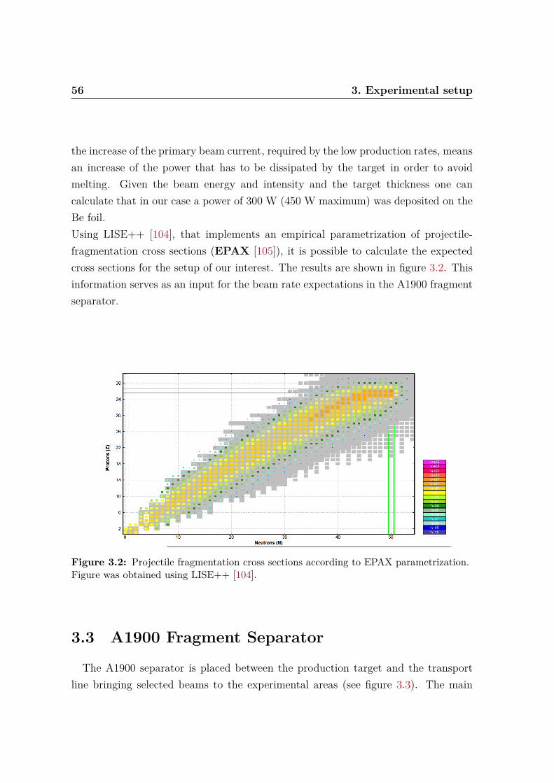
56 3. Experimental setup
the increase of the primary beam current, required by the low production rates, meansan increase of the power that has to be dissipated by the target in order to avoidmelting. Given the beam energy and intensity and the target thickness one cancalculate that in our case a power of 300 W (450 W maximum) was deposited on theBe foil.Using LISE++ [104], that implements an empirical parametrization of projectile-fragmentation cross sections (EPAX [105]), it is possible to calculate the expectedcross sections for the setup of our interest. The results are shown in figure 3.2. Thisinformation serves as an input for the beam rate expectations in the A1900 fragmentseparator.
Figure 3.2: Projectile fragmentation cross sections according to EPAX parametrization.Figure was obtained using LISE++ [104].
3.3 A1900 Fragment Separator
The A1900 separator is placed between the production target and the transportline bringing selected beams to the experimental areas (see figure 3.3). The main

3.3 A1900 Fragment Separator 57
Figure 3.3: Schematic view of the Coupled Cyclotron Facility connected to the A1900fragment separator. Adapted from [106].
purpose of this tool is to select the requested ions among the huge variety of sta-ble and radioactive species produced by the fragmentation reactions in the primarytarget [106]. The A1900 fragment separator was commissioned in 2001 [107] andtook the place of the previous A1200 device [108]. With respect to the older one,the new tool has higher angular and momentum acceptance and a better resolvingpower. Details can be found in table 2 of [107]. Moreover, the A1200 had collectionefficiencies in the few percent range, while in selected cases efficiencies approaching100% are possible with the new device. This can accept over 90% of a large range ofprojectile fragments produced at the NSCL.The A1900 relies on superconducting iron-dominated quadrupole magnets workingat liquid Helium temperature. The setup is composed of 40 large-diameter supercon-ducting multipole magnets and four 45 dipoles. The maximum magnetic rigidity is6 Tm. From the optical point of view, the A1900 has three intermediate images. Ac-cess to the first image is limited by a thick steel shielding wall and contains a beamstopper. A degrader is placed at the second image along with high rate detectorsand aperture plates to define the momentum acceptance. The third image occursin a large vacuum box fitted with continuously adjustable slits to better define thebeam acceptance. The focal plane of the machine is the injection point for the beamtransport lines that bring the selected ensemble of beams to the experimental areas.At this position the scintillator called ”xfp“ is placed. This detector will be used inthe data analysis for the incoming beam particle identification, as described later.For fragments with relativistic velocities, a separation by mass and nuclear charge

58 3. Experimental setup
is not possible with the sole use of magnetic or electric fields. To achieve beampurification and isotopic selection, the A1900 uses a separation method based onmagnetic-rigidity analysis and energy loss degrader material.The admixture of unreacted and fragmented ions are first filtered to select a singlemagnetic rigidity by the initial dispersive beam line in conjunction with an apertureat image 2. In this step also the momentum acceptance (dp/p) is defined acting on theslit aperture at image 1 and 2. Isotopic separation is then completed by passing theions through an energy degrading ”wedge“, from which ions entering with a single Bρ
but with different atomic numbers emerge with different momenta. This is requiredto separate ions of different species but with similar velocities (that is quite the case ofnuclear fragmentation products) and same A/q ratio. The following dispersive beamline then provides, in most cases, isotopic separation. The nature and thickness ofthe energy degrader, as well as the size of momentum apertures, are parameters thatare adjusted to control the secondary beam intensity and purity. This technique hasbeen used to provide secondary beams with E/A as low as 30 MeV. However, thebest purities and yields have been obtained at significantly higher energies.In most cases it is not possible to select one single isotopic species from the frag-mentation products since these have similar masses, velocities and A/q ratio. Forthis reason, in several circumstances, an ensemble of secondary beams is transportedto the experimental hall. This is the so-called ”cocktail beam“. From the point ofview of the experiment, it might be necessary to tag the beam particles prior to theirarrival on the secondary target measuring their mass and charge as well as their mo-mentum.For the experiment we are interested in, an Al wedge 240 mg/cm2 thick was used.With this setup, the optimal beam momentum spread for the particles tagging isdp/p = 0.5% and this was used in the present experiment for the beam tuning. Dueto the low production cross sections of strongly exotic 74Ni, this parameter limitsthe beam current intensity, preventing the feasibility of a Coulomb excitation exper-iment in a reasonable time. For this reason the choice of running at dp/p = 3.0%
was needed. However we shall see in the next chapter how this affects the incomingbeam identification.The 74Ni rates predicted by the LISE++ calculation resulted a factor 6 higher thanthe measured one. During the experiment, an average rate of ≈ 0.7 pps was measured.

3.4 S800 spectrometer 59
3.4 S800 spectrometerThe S800 [109] is a large acceptance, high-resolution spectrometer designed for
experiments using radioactive beams produced by projectile fragmentation. It relieson superconducting magnets and it is composed of three main parts: the AnalysisLine, the Spectrometer itself and the Focal Plane Detectors. A sketch of the completedevice is shown in figure 3.4.
Figure 3.4: Schematic view of the S800 spectrometer: the three main components ofthe device are shown. The beam particles enter the analysis line on the left and hit thesecondary target where the CAESAR array has been placed. Scattered particles are thenanalyzed by the actual S800 spectrometer and measured by the focal plane detectors.Adapted from [110].
The Analysis line is made of several optical elements used for different purposes:tuning the secondary beams on the reaction target, implementing different opticalmodes and, in some cases, measure the characteristics of the incoming particles. It ismade of two couples of dipoles and 5 quadrupole triplets with a maximum rigidity of4.9 Tm corresponding to 800 MeV protons. At the very beginning of the Analysis line,at the ”Object“ position, a 125 µm (or thicker) plastic scintillator is placed across thebeam path. This is called the “Object scintillator” (obj) and timing information fromthis device will be used in the data analysis for the incoming particle identification.

60 3. Experimental setup
The actual S800 spectrometer part consists of a high-resolution and high-acceptancespectrometer made of two superconducting dipoles spanning from the target positionto the focal plane. It has an angular acceptance of ±5 deg in the non dispersiveand of ±3.5 deg in the dispersive directions, totalling a solid angle of 20 msr. Themaximum rigidity of the magnets is 4 Tm and the momentum acceptance is about±3%. Depending on the experimental setup, the performance can vary. Typicalresolution for radioactive beams is 1 part in 2000 in energy and 10 mrad in scatteringangle but the nominal resolution is much higher (1/104) and requires to use verysmall beam spots (≈ 0.5 mm in diameter). As discussed in [111], from the opticalpoint of view the S800 can be operated in three different modes:
• in the dispersion matched mode the momentum spread of the beam at theobject position is canceled at the focal plane but this means that the beammomentum is dispersed at the target position. In this mode the whole S800(analysis line and spectrometer) is achromatic.
• in the focused mode the beam is focused on the target and the momentum isspread at the focal plane. This mode allows large momentum acceptance.
• monochromatic mode. This mode requires the fabrication of a mono-energeticwedge to be placed at the intermediate image and is used to produce very lowenergy beams.
In the present experiment the focused mode was used since it has been necessaryto run at large momentum acceptance. In this operating mode, the cocktail beamcoming from the A1900 and running along all the transport line is focused at theobject position. From here the beam is transported along the analysis line of the S800and reaches the target in a position very close to the pivot point of the spectrometer.After the target a quadrupole focusing doublet is used to re-focus the scattered andnon-scattered particles and inject them into the spectrometer dipoles. Here the ionsare dispersed along one direction according to their A/q ratio. At the focal plane ofthis device a set of detectors is used for energy measurement and track reconstruction.The tuning of the magnetic field of the dipoles allows to center the reactions productsof interest on the focal plane, thus selecting the desired reactions channels. In theexperiment we are discussing, the main interest is to measure 74Ni ions exiting the

3.5 S800 Focal Plane Detectors 61
target with a velocity β ≈ 0.36, this means Bρ ≈ 3.2 Tm. In the final measurementsetting a Bρ value of 3.19 Tm was used.
3.5 S800 Focal Plane Detectors
Figure 3.5: Schematic view of the S800 focal plane detector arrangement. Particles dis-persed by the S800 dipoles enter the gas volume (in yellow) from the right side of theplot. After passing through the 2 CRDC detectors, the ions encounter the IonizationChamber (in blue) and the e1 scintillator (in red). Adapted from [112].
The S800 setup is equipped with three different types of detectors placed at thefocal plane of the spectrometer [112]. These have to be properly optimized to achievehigh-resolution performance exploiting the high optical resolution of the spectrometeritself. First of all, a couple of Cathode Readout Drift Chambers (CRDC) is used tomeasure the particle x-y position. Afterwards, a segmented ionization chamber servesfor the ions energy measurement acting as a ∆E detector. The last step is made ofthree thick plastic scintillators used for the residual energy measurement, timing
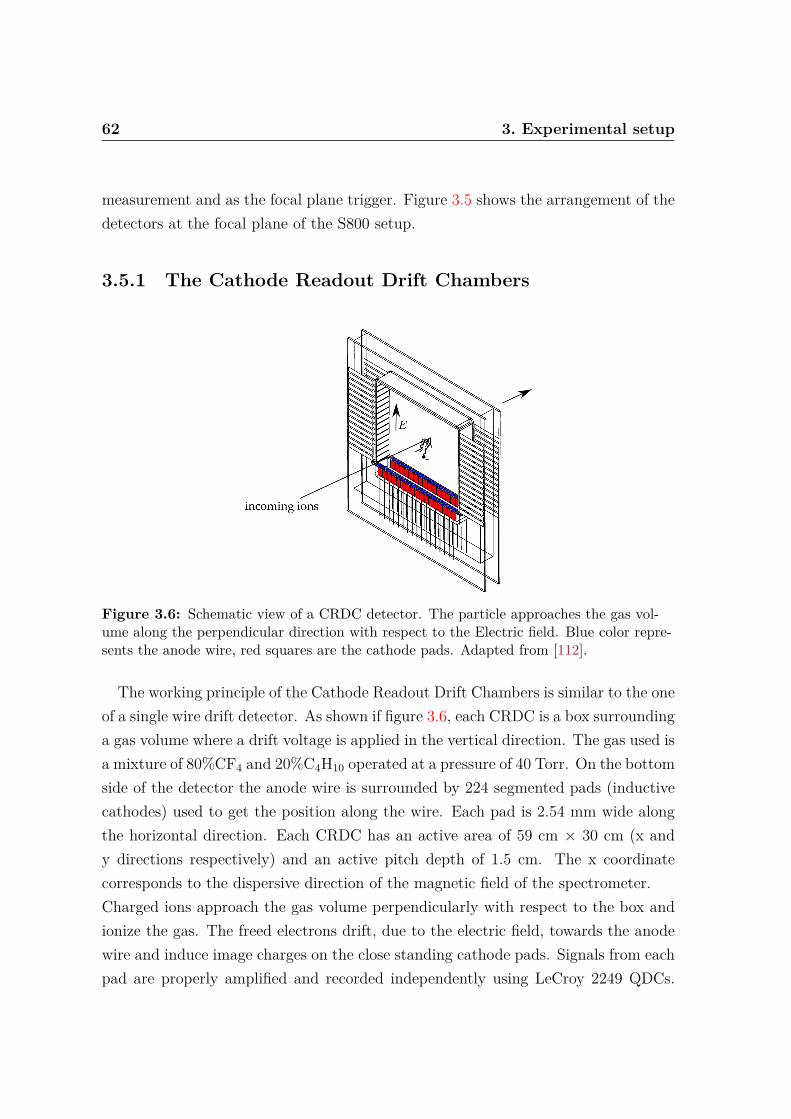
62 3. Experimental setup
measurement and as the focal plane trigger. Figure 3.5 shows the arrangement of thedetectors at the focal plane of the S800 setup.
3.5.1 The Cathode Readout Drift Chambers
Figure 3.6: Schematic view of a CRDC detector. The particle approaches the gas vol-ume along the perpendicular direction with respect to the Electric field. Blue color repre-sents the anode wire, red squares are the cathode pads. Adapted from [112].
The working principle of the Cathode Readout Drift Chambers is similar to the oneof a single wire drift detector. As shown if figure 3.6, each CRDC is a box surroundinga gas volume where a drift voltage is applied in the vertical direction. The gas used isa mixture of 80%CF4 and 20%C4H10 operated at a pressure of 40 Torr. On the bottomside of the detector the anode wire is surrounded by 224 segmented pads (inductivecathodes) used to get the position along the wire. Each pad is 2.54 mm wide alongthe horizontal direction. Each CRDC has an active area of 59 cm × 30 cm (x andy directions respectively) and an active pitch depth of 1.5 cm. The x coordinatecorresponds to the dispersive direction of the magnetic field of the spectrometer.Charged ions approach the gas volume perpendicularly with respect to the box andionize the gas. The freed electrons drift, due to the electric field, towards the anodewire and induce image charges on the close standing cathode pads. Signals from eachpad are properly amplified and recorded independently using LeCroy 2249 QDCs.

3.5 S800 Focal Plane Detectors 63
Several methods for determining the x coordinate of the particle trajectory have beentested [112]: simple center of gravity of all the pads, the center of gravity of severalpads around the peak and a Gaussian fit of the charge distribution were compared.The fit of the peak was found to be the best method, allowing to reach the 0.5 mmresolution required to fully exploit the resolving power of the spectrometer.The y coordinate is obtained by measuring the electron drift time inside the CRDC.The start signal is given by the arrival of the particle in the e1 scintillator, while thestop is the signal induced at the anode by the drifted electrons. The calibration ofthe x and y coordinates will be discussed in the next chapter.
3.5.2 Particle trajectory reconstruction
Figure 3.7: Trajectory reconstruction at the focal plane. The positions measured bythe CRDCs allow to calculate the angles at the focal plane in the dispersive and non-dispersive directions of the spectrometer (ata, bta respectively).
Two CRDC detectors are housed in the same gas volume and placed 1 m apart inthe beam direction (z) (see figure 3.5).Combining the (x1, y1) and (x2, y2) position information measured by the two CRDCsit is possible to reconstruct the particle trajectory at the focal plane. As shown

64 3. Experimental setup
in figure 3.7, one can define the dispersive and non-dispersive focal plane anglesrespectively as:
afp = arctan
[x2 − x1
∆z
](3.1)
bfp = arctan
[y2 − y1∆z
](3.2)
where ∆z= 1000 mm is the (fixed) gap between the two detectors. Using as focalplane the ”image“ of CRDC1, the position at the focal plane (xfp, yfp) coincides withthe position (x1, y1) measured by CRDC1 itself. Since the optics of the spectrometeris known, given the Bρ parameters, Z and A of the particle and the measured tra-jectory at the focal plane, it is possible to reconstruct the particle trajectory at thetarget position using the inverse map S−1 of the S800. This can be obtained usingthe COSY-Infinity code as described in [113]:
ata
yta
bta
dta
= S−1
xfp
afp
yfp
bfp
(3.3)
Here ata and bta are respectively the dispersive and non-dispersive angles recon-structed at the target, yta is the reconstructed y position at the target and dta is thefractional deviation in kinetic energy of the particle (E) from the kinetic energy ofthe same particle taking the central path through the spectrograph (E0):
dta =E − E0
E0
(3.4)
Given the experimental parameters and the ion of interest, the inverse map can beautomatically calculated and retrieved from [110]. The dispersive and non-dispersiveangles reconstructed at the target can be used to calculate the laboratory scatteringangles θ and ϕ:
θ = arcsin√sin2(ata) + sin2(bta) (3.5)
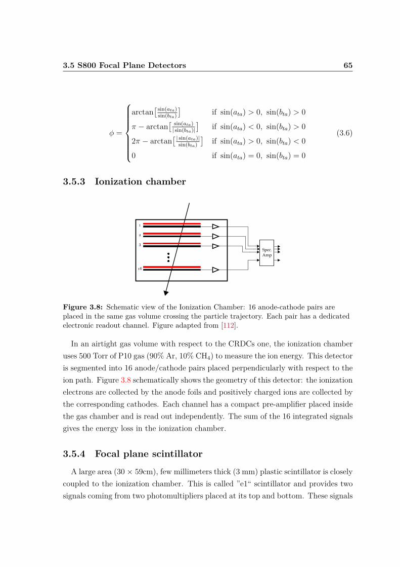
3.5 S800 Focal Plane Detectors 65
ϕ =
arctan[sin(ata)sin(bta)
]if sin(ata) > 0, sin(bta) > 0
π − arctan[ sin(ata)| sin(bta)|
]if sin(ata) < 0, sin(bta) > 0
2π − arctan[ | sin(ata)|
sin(bta)
]if sin(ata) > 0, sin(bta) < 0
0 if sin(ata) = 0, sin(bta) = 0
(3.6)
3.5.3 Ionization chamber
1
2
3
16
Spec.Amp
Figure 3.8: Schematic view of the Ionization Chamber: 16 anode-cathode pairs areplaced in the same gas volume crossing the particle trajectory. Each pair has a dedicatedelectronic readout channel. Figure adapted from [112].
In an airtight gas volume with respect to the CRDCs one, the ionization chamberuses 500 Torr of P10 gas (90% Ar, 10% CH4) to measure the ion energy. This detectoris segmented into 16 anode/cathode pairs placed perpendicularly with respect to theion path. Figure 3.8 schematically shows the geometry of this detector: the ionizationelectrons are collected by the anode foils and positively charged ions are collected bythe corresponding cathodes. Each channel has a compact pre-amplifier placed insidethe gas chamber and is read out independently. The sum of the 16 integrated signalsgives the energy loss in the ionization chamber.
3.5.4 Focal plane scintillator
A large area (30 × 59cm), few millimeters thick (3 mm) plastic scintillator is closelycoupled to the ionization chamber. This is called ”e1“ scintillator and provides twosignals coming from two photomultipliers placed at its top and bottom. These signals

66 3. Experimental setup
are used to obtain position, timing and energy information. Due to the fast responseof this detector it is used for three different tasks:
• as a time reference for the electrons drift time in the CRDCs;
• it is the reference for time of flight measurement of the particles along the S800analysis line (obj scintillator) and from the A1900 focal plane (xfp scintillator);
• it is the main trigger source of the S800 focal plane detectors.
3.6 CAESAR arrayCAESAR [114] is an array of 192 CsI(Na) thick scintillators specifically designed
for in beam γ-ray spectroscopy in the intermediate energy domain. This is compara-ble to the most common NaI(Tl) in terms of energy resolution, timing performanceand costs but it has a 30% higher stopping power for γ-rays. In situations like the oneof our interest, where the 74Ni beam intensity is extremely low, the gamma detectionefficiency becomes a crucial parameter for the feasibility of the experiment. AlthoughHigh-Purity Germanium (HPGe) is still the material of choice for the construction ofγ-ray spectrometers, the efficiency performance and angular coverage reachable withan array of scintillators triggered the development of the setup that we will describein the following.Due to the typical velocities of the reaction recoils (β ≥ 0.3), the de-excitation gammarays are Doppler-shifted with respect to their original energy. For this reason one hasto perform Doppler correction in order to obtain the proper de-excitation spectrum.In the design of CAESAR the goals of more than 95% solid angle coverage and a total40% efficiency for 1 MeV γ-rays were achieved. Intrinsic energy resolution is ≈ 7%FWHM for 1 MeV photons. Considering the solid angle subtended by each crystal,the effective energy resolution in an in-beam experiment, which includes the effects ofDoppler broadening, reduces to ≈ 10%. Given these values, one could discuss whereand how an appreciable gain in global detection efficiency and angular coverage isworth despite the energy resolution. For the present experiment the answer is ob-vious, given the extremely reduced number of measured 74Ni de-excitation photons(less than 100) that would reduce by a factor ten using standard HPGe detectors.For the sake of completeness one has to say that the advent of the new generation of

3.6 CAESAR array 67
gamma-ray tracking arrays like AGATA [115] and GRETINA [116] has completelyaltered the panorama offering extreme energy resolution combined with good effi-ciency. Costs and complexity are however orders of magnitude far from the setup weare describing.It should be added that during the CAESAR design study the possibility to useLaBr3:Ce scintillating materials was also investigated. This solution would have ledto a higher detection efficiency and superior timing performances maintaining thesame quality for in beam γ-ray energy resolution. The unavoidable drawback wouldhave been the cost of such detectors to achieve the required CAESAR angular cov-erage and granularity.The geometry of the array was decided according to several constraints that a GEANT4simulation helped to define. First of all the γ-ray detection efficiency had to be max-imized and particular care had to be put at the forward angles where, due to theLorentz boost, the angular distribution is expected to peak. Moreover, geometricalspace limitations, the required granularity and the possibility to couple the detectorsto commercially available photomultiplier tubes have been taken into account.The final choice was to arrange 192 detectors shaped as rectangular parallelepipeds in10 rings (A..J) perpendicular to the beam axis. Two different sizes of detectors whereused. Size 1 is 3.13 × 3.13 × 3 inches, while size two is 2.13 × 2.13 × 4 inches. Theirarrangement in rings is reported in table 3.2, while a geometrical sketch is shown infigure 3.9.
Ring Number of det. sizedetectors type
A 10 1B 14 1C 24 2D 24 2E 24 2F 24 2G 24 2H 24 2I 14 1J 10 1
Table 3.2: CAESAR detectors arrangement.

68 3. Experimental setup
The hygroscopic CsI(Na) scintillation crystals are placed in an aluminum housingwith a 1 mm wall thickness. A reflective material fills the 1.5 mm gap between thecrystal and the wall of the aluminum housing. The latter is sealed with a borosilicatewindow through which the photomultiplier is coupled.The spectroscopy photomultiplier tubes R1306 and R1307 from Hamamatsu are usedfor the two different crystal sizes. A passive voltage divider board distributes theexternally applied high voltage to the dynodes. Since CAESAR has to operate closeto the S800 spectrometer, in an area where the magnetic fringe fields of the S800entrance quadrupole are not completely shielded, a proper shielding for the magneticfields had be implemented. This is done by covering the photomultiplier tubes, insidetheir housing, with multiple layers of µ-metal. It was verified that this shieldingprovides proper operation up to 2-3 Tm external field. It was also measured thatalready 0.5 Tm of unshielded magnetic fields affect the output pulse height.
The photomultiplier tube with magnetic shielding and Al housing fits within the
Figure 3.9: CAESAR geometry. Left panel shows the cross-sectional view of the CAE-SAR array along the beam direction for rings J and F. Right panel shows the cross-sectional view parallel to the beam axis of the entire setup. Adapted from [114].
shape of the crystal enclosure, thus detectors can be placed close to each other withoutany significant gap in between. Figure 3.10 shows a picture of the final assembly, whilea picture of the complete CAESAR setup mounted at the secondary target positionis shown in figure 3.11.Each detector has a dedicated power supply line that provides positive high voltageto the respective photomultiplier. The high voltage tuning is used both to match the

3.6 CAESAR array 69
output signals amplitude and to set the dynamic range of the setup. A broad intervalcan be spanned going from 1 to several tens of MeV of full scale energy. In Coulombexcitation experiments with fast beams, typically a dynamic range of 8 MeV is used.
Figure 3.10: Picture of the final assembly of one CAESAR detector. Adapted from[114].
3.6.1 CAESAR Electronics
A specific high speed data acquisition system has been developed for the CAESARsignals readout. A scheme of the electronics is reported in figure 3.12. The core of thesystem are the LeCroy Fast Encoding Readout ADCs (FERA) 4300 CAMAC mod-ules [117]. Raw signals coming from the detectors (PMTs output) are split into twobranches: the energy and the time branch. This is done using a dedicated module(PicoSystem splitter-and-amplifier) that performs a fixed gain fast amplification andprovides two outputs for each input.The energy branch signals are sent to custom shaping amplifiers with variable gainand fixed shaping time (4 µs). The amplified signals are then delivered to the inputsof the 4300B FERA QDCs that are operated effectively as peak sensing ADCs. Thisis done by integrating the long-tail-shaped-signals coming from the amplifiers in a 25ns time gate applied at the maximum of the signal. The integration gate is handledin a common way by the FERA 4301 driver and depends on the S800 trigger logic.The time branch signals are sent instead to 12 RIS 13080 Constant Fraction Dis-criminator modules. Each module handles 16 channels and is operated in the two-thresholds mode. The lower threshold of the CFD is used to decide whether to acceptor not a signal, while the higher threshold is used to select higher energy events for

70 3. Experimental setup
Figure 3.11: A photograph of the CAESAR array mounted at the pivot point of theS800 spectrometer.
the trigger request. The global CAESAR trigger is then the OR of the lower thresh-old CFD outputs validated by the OR of the higher ones. This means that eachCAESAR event will contain at least one detector with a signal exceeding the higherthreshold and all the signals exceeding the lower one. The single output of each CFDchannel is then delayed by 500 ns using cable ribbons and, after, is acquired by the4303 Time to FERA Converters (TFC). Those modules are operated in common startmode where the start is given by the master trigger and the stop is the individualdiscriminated signal. The output of the TFCs is a NIM signal, the width of whichbeing proportional to the measured time. This is successively acquired using the4300B FERA QDCs with a 500 ns fixed integration gate.The data recorded by the energy-branch and time-branch QDCs are readout fromthe FERA drivers. This is done using two FPGA modules that provide the interfacebetween the FERA world and a VME Crate where the NSCL standard acquisition

3.6 CAESAR array 71
system has access. As already stated, the main CAESAR trigger is evaluated usingthe CFDs OR. Since this device is operated in conjunction with the S800, the realtrigger for the FERA modules comes from the trigger module of that setup: the trig-ger request is sent from CAESAR to the S800 trigger logic and an evaluated mastertrigger is received back. The latter is the actual CAESAR trigger.
Figure 3.12: CAESAR readout electronics scheme.
3.6.2 Add-back procedure
At the γ-ray energies considered in the present work, Compton scattering is thedominant effect (for a detailed description of the interactions of photons with matterin this energy domain see [118–120]). Even using thick scintillation crystals, thereis a non-zero probability that Compton scattered γ-rays escape the active volume ofthe detector, releasing only part of their initial energy. Looking at a single-detectorenergy spectrum, this effect produces the so-called ”Compton Continuum“. In the

72 3. Experimental setup
limit of single Compton scattering, the Compton continuum extends from zero up to≈ Eγ-250 keV, which can be estimated considering a backward scattering in the wellknown Compton scattering formula:
E ′γ =
Eγ
1 + Eγ
mec2(1− cos(θ))
(3.7)
where Eγ and E ′γ are respectively the incident and scattered photon energies, θ
is the laboratory scattering angle and mec2 is the rest mass of the electron (0.511
MeV/c2). Multiple scatterings modify the shape of the continuum, which practicallyextends up to the full-energy peak. If the scattered photon escapes from the detector,the information about the total incoming energy is lost and the photo-peak efficiencyis therefore affected.One of the techniques that can be applied in order to recover part of these events isthe nearest neighbor add-back. The idea is to see if the escaping photon has releasedenergy in one of the detectors neighboring the one that was first hit, in order toreconstruct the initial total energy by summing up the partial contributions. Fromthe practical point of view, given the geometry of the array and the size of thescintillators, it is a reasonable approximation to limit the discussion to the casewhere no more than two neighboring detectors were hit. The add-back procedure iscomputed as follows:
• browse all the detectors and select those that have been hit;
• consider each selected hit and count how many of its neighbors were also hit.This can give three different results:
n0: No neighbors were hit: the present hit is taken as it is;
n1: One neighbor was hit: the energy from the two detectors is summed upand assigned to the detector with the higher energy deposit;
ng: More than one neighbor was hit: discard the hits.
• The energy spectrum is filled with the n0 (raw) and n1 (reconstructed) hits.
The effect of the add-back procedure applied to a 88Y calibration source is clearlyvisible in figure 3.13. The calibrated and integrated CAESAR spectrum shown areobtained with and without the use of the routine. The add-back is clearly reducing

3.6 CAESAR array 73
the Compton background and increasing the photo-peak efficiency. The efficiencygain has been quantified using activity-calibrated sources and will be discussed inthe next paragraph. It is important to underline that the experimental conditions ofa calibration run are quite different with respect to the in-beam case where a hugeatomic background can affect the quality of the event reconstruction. In the nextchapter we will show how this contamination affects the present data analysis.
Energy (keV)0 500 1000 1500 2000 2500 3000 3500
coun
ts /
4 ke
V
0
5000
10000
15000
20000
25000
30000
35000
40000
45000
Add-back: ON
Add-back: OFF
Figure 3.13: Measured γ-ray spectrum of a 88Y source. The red line is the sum of thecalibrated single-detector spectra for the 192 scintillators; the blue line shows the gain inphoto-peak efficiency after the add-back procedure has been applied.
3.6.3 Performance of CAESAR
CAESAR was commissioned in 2009 and the performance obtained both with sta-tionary sources and in a Coulomb excitation experiment are reported in [114]. Figure3.14 shows the measured global resolution in terms of peak FWHM. Data obtainedfrom in-beam experiments and using stationary sources are compared to show how

74 3. Experimental setup
the Doppler reconstruction of the γ-rays emitted by a fast moving source (β=0.37)affects the effective resolution. In figure 3.15 one can see the gain in efficiency thatcan be achieved when applying the add-back procedure to the data measured withstationary sources. For the ≈ 1 MeV photons of interest in the present work, theexpected full-energy peak efficiency is ≈ 30% if no add-back is performed and ≈ 35%using add-back. Since the velocity of the scattered 74Ni will be close to the one of thereference (β ≈ 0.36), the expected in-beam resolution is about 10% FWHM. Theseparameters have been re-measured while calibrating CAESAR for the experimentand while setting the energy thresholds. The latter have been kept quite high (≈ 300keV) since the energy region of interest is at 1 MeV and typical Coulomb excitationexperiments are affected by a huge low energy background due to atomic processesand Bremsstrahlung radiation. Energy thresholds are strongly related to the actualdetection efficiency. In order to quantify these effects a GEANT4 simulation wasdeveloped [121] and will be used for the data analysis.
Figure 3.14: In-beam and intrinsic energy resolution (FWHM) as measured from stan-dard calibration sources and in an intermediate-energy Coulomb excitation experiment.The in-beam part was obtained after Doppler reconstruction of the γ-rays emitted bysources with velocity β = 0.35. Adapted from [114].

3.6 CAESAR array 75
Figure 3.15: Absolute full-energy-peak efficiency of CAESAR measured with calibrationsources. Results are compared with and without add-back. Adapted from [114].

76 3. Experimental setup

4Data Analysis
In this chapter, the data analysis of experiment 09031 performed at NSCL is re-ported. The experimental setup was described in chapter 3, here we will focus on thedetector calibration and on the following data analysis.The final goal is to extract the Coulomb excitation cross section for the first 2+ stateof the 74Ni nucleus using the reaction 74Ni + 197Au at ≈ 90 AMeV.The experimental cross section is given by:
σ0+→2+ =Nγ
2+→0+
NB NT
(4.1)
where the main ingredients are:
• Nγ2+→0+ : number of de-excitation γ-rays;
• NB: number of 74Ni projectiles approaching the secondary target and reachingthe S800 focal plane without undergoing nuclear reactions;
• NT : areal density of the 197Au target.

78 4. Data Analysis
In the following we will show how these values have been obtained from the exper-imental data.An important part of the work was performed using a custom NSCL software de-veloped in the ROOT [122] framework by K. Wimmer [123]. This code providesthree main tools. The first allows to unpack the raw data from the NSCL binaryformat to non-calibrated ROOT Trees. The second contains some automated orsemi-automated calibration procedures and the third allows to apply the calibrationfactors, producing calibrated ROOT Trees. An event by event analysis was laterperformed on these data to obtain the required cross section.We will first describe the calibration of the S800 focal plane detectors and of theCAESAR detectors. After this, the particle identification process and the particlestrajectory reconstruction will be discussed. Using this information, the γ-ray spec-trum will be used to extract the cross section value.
4.1 Focal plane detectors calibration
The calibration of the Focal plane detectors has to be performed keeping in mindwhat kind of information is needed for the following analysis.The focal plane scintillator will only be used as a time reference for the Time OfFlight of the ions, therefore no absolute calibration is needed.The ionization chamber provides the ∆E information for the particle identificationat the focal plane (see par. 4.5). This value is obtained by summing up the 16 signalscoming from the different segments of the detector. Even if an absolute energycalibration of the ∆E is not needed, a proper gain match of the 16 channels has to beperformed before the signals can be added. The left panel of figure 4.1 shows the rawenergy-loss spectra as a function of the segment number. Segment 1 was arbitrarychosen as a reference and a linear function was used to shift the data of the othersegments.
The calibration parameters for each segment are obtained selecting different iso-topes on a roughly calibrated particle identification spectrum and fitting the particlegated energy projections. As it can be seen in figure 4.2, since the energy loss in thegas differs according to the atomic species, each particle-gate provides one calibra-tion point. The linear regression of the measured centroids of the distributions with

4.1 Focal plane detectors calibration 79
Figure 4.1: Gain matching procedure: the two panels show the energy loss measuredby the Ionization Chamber as a function of the segment number before (left) and after(right) the gain matching procedure.
respect to the reference values gives the parameters for the linear segment matching.This procedure is repeated for all the segments and the result is shown in the rightpanel of figure 4.1. At this point the corrected values can be summed up to obtainthe total energy loss in the ionization chamber.
raw energy (channels)600 800 1000 1200 1400 1600 1800 2000 2200
coun
ts
0
200
400
600
800
1000
1200
Zn77
Cu75
Ni74
Figure 4.2: Ionization chamber equalization procedure. The energy loss peaks gatedon different isotopes for the segment to be aligned (blue) are shifted to the reference one(red) according to a linear calibration.
The CRDC detectors are processed in two steps. First, a gain matching of thesingle-pad signals is needed. The procedure is equivalent to what was shown for the

80 4. Data Analysis
Ionization Chamber. Once this is done, the absolute position calibration has to beobtained. Since the CRDCs will be used for the particle trajectory reconstructionat the focal plane (see par. 3.5.2), an absolute calibration of the x and y variablesof the two detectors is needed. This is done by masking each CRDC with a thickTungsten shielding with several holes at known (x, y) positions. The geometry ofthe used mask is shown in figure 4.3. A few minutes of dedicated beam-runs haveto be performed for each CRDC and this method is usually referred to as the MaskCalibration. The procedure has to be periodically repeated during the experimentto account for long-term drifts due to gas pressure or electric field fluctuations. Atypical Mask Calibration spectrum is shown in figure 4.4.
Figure 4.3: Schematic view of the mask used for the CRDC calibration. Adapted from[124].
The calibration factors for the y axis are extracted from a linear interpolation of themeasured peaks with respect to the nominal holes positions. This allows to accountfor the variation of the parameters affecting the electron velocity in the gas (i.e. gaspressure and temperature) and for the offset in the time measurement relative to thee1 scintillator. Since the readout of the x axis is performed using the cathode pads,that are fixed in space, the gain of this axis (represented by the slope of the linearcalibration) is fixed and is equal to the size of one pad (2.54 mm), therefore for thisaxis only the offset (intercept) has to be determined.The calibration factors have been applied to the measured data using the closestMask Calibration run available (in time).

4.1 Focal plane detectors calibration 81
raw X position (ch)20 40 60 80 100 120 140 160 180 200 220
Nu
mb
er o
f E
ntr
ies
0
10
20
30
40
50
60
Figure 4.4: Top: measured data for the calibration of CRDC1. Bottom: x axis projec-tion of the central holes line.

82 4. Data Analysis
4.2 CAESAR calibrationThe calibration of the 192 CsI(Na) CAESAR detectors was performed using stan-
dard calibration sources. Prior to the experiment, a gain matching of the signalscoming from the detectors was done optimizing for each channel the correspondingpower supply voltage and the amplifier gain.
4.2.1 Energy and Time Calibration
For the energy calibration of the CAESAR detectors, runs with the 60Co, 88Y, 137Csand 22Na sources were used. A dedicated tool was developed to automatically fit thecalibration runs and manually check the results. When the automatic procedurefails, the software allows to manually re-fit the peak. A second order polynomial wasused to fit the calibration data. Figure 4.5 shows a screen-shot of the software usedwhile figure 4.6 displays the calibration curve for one detector. A global view of thecalibration consistency for the whole CAESAR array is given in figure 4.7.The time spectra used in the data analysis are given by the difference between theCAESAR time measured by the TFCs and a reference signal (i.e. the OBJ scintillatortime). Although timing resolution is not a priority for the present experiment, therelative offset between the detectors has to be matched to obtain proper time-gateconditions. To do this, the offset of each channel was evaluated with respect to achannel chosen as a reference. The obtained values were used as the time calibrationparameters.
4.2.2 Energy resolution
The energy-calibrated spectra have been also used to estimate the energy resolutionof the CAESAR detectors. The measured Gaussian peak width (σ) as a function ofthe energy are shown in figure 4.8. The data refer to the CAESAR-summed spectrumwith and without the use of the add-back routine. It can be seen that the add-backworsens the energy resolution by a factor close to 3% for 1 MeV γ-rays. The resolutionof each detector has been used as an input parameter for the simulation that will be

4.2 CAESAR calibration 83
Figure 4.5: Screen-shot of the calibration software used to verify and correct the auto-matic fit results.
Figure 4.6: Calibration curve for a typical detector, the blue line is the fitted polyno-mial.
described in paragraph 4.3. According to the parametrization used by the simulation,

84 4. Data Analysis
Figure 4.7: 88Y source energy spectrum as a function of the detector number
the energy dependence of the peak width has been fit using the following formula:
σ(E) = α · Eβ (4.2)
Typical values of α and β are of the order of 0.60 and 0.55 respectively. In figure4.9 the measured percentage resolution is shown as a function of the γ-ray energy. Agood agreement is found with respect to the CAESAR published data [114] discussedin 3.6.3.
4.2.3 Energy thresholds
Another parameter that has to be taken into account is the energy threshold of thedetectors. As already stated in the previous chapter, Coulomb excitation experimentswith radioactive beams at intermediate energy are affected by a huge backgrounddue to atomic processes between the cocktail beam and the heavy thick target used.Since the excitation cross section depends on the square of the atomic number of thereaction partner (σex
p,t ∝ Z2t,p, cfr. eq. 2.34), the use of thick and high Z materials is
useful to compensate for the low beam intensity and the low excitation cross sections

4.2 CAESAR calibration 85
Energy (keV)400 600 800 1000 1200 1400 1600 1800
(E
) (k
eV)
σ
20
25
30
35
40
Add-back: on
Add-back: off
Figure 4.8: Measured resolution of the CAESAR array as a function of the γ-ray en-ergy. Blue (red) dots are the measured data with (without) the use of the add-back rou-tine. The corresponding lines are obtained using the function of eq. 4.2.
one has to deal with. The unavoidable drawback are the photons emitted by atomicprocesses that produce a continuum background up to several hundreds of keV. Sincethe energy of the transition of interest for the present measurement is of 1024 keV, toavoid an excessive count-rate due to the mentioned background, the trigger thresholdsof the CAESAR detectors were set to a value of ≈ 300 keV. These thresholds affectthe detection efficiency, especially when the add-back procedure is applied and haveto be taken into account. To do this, 133Ba source runs with lowered thresholds werecompared to the experimental condition. Figure 4.10 shows this comparison for oneof the CAESAR detectors. The measured thresholds were used as an input for thesimulation that we will describe in the following paragraph.

86 4. Data Analysis
Energy (keV)400 600 800 1000 1200 1400 1600 1800
FW
HM
(%
)
5
5.5
6
6.5
7
7.5
8
8.5
9
9.5
Add-back: on
Add-back: off
Figure 4.9: Intrinsic percentage energy resolution of the CAESAR detectors (FWHM%) as measured with standard calibration sources.
4.3 GEANT4 simulation
As anticipated in the previous paragraphs, a GEANT4 [125] simulation of theCAESAR array has been implemented at NSCL by T. Baugher [121] and will beused in the present analysis to fit the final γ-ray spectra. This code implements thegeometry of the CAESAR array and has been used to simulate the energy release ofthe γ-rays in the active volume of the detectors. The use of a simulation allows for aproper detection efficiency estimation at the energy of interest. Moreover, it allowsto disentangle the different contributions to the γ-ray spectrum coming from sourcesemitting at different velocities and to take into account the effects on the energyresolution due to the Doppler correction. Indeed, both stationary sources and in-beam conditions can be simulated. In the first case, a source of a given energy shootsγ-rays isotropically towards the detectors, while in the in-beam condition a projectilewith given kinetic energy is shot towards the target. In this case, the interaction of

4.3 GEANT4 simulation 87
Energy (keV)100 150 200 250 300 350 400 450 500
No
rm. c
ou
nts
(a.
u.)
0
0.2
0.4
0.6
0.8
1 Low Threshold
Exp Threshold
Ba133
Figure 4.10: Energy threshold evaluation using the 133Ba source. Blue line: experimen-tal threshold condition. Red line: lower threshold condition. See text for details.
the particle with the target material is taken into account and the tracking of theincident particle is performed. If the target/projectile excitation option is turned on,a γ-ray of the selected energy is shot by the excited particle considering its momentumat the time of emission (causing the Doppler-shift of the photon).In both cases (stationary source or in-beam condition), the simulation tracks the γ-ray path recording the energy release in the CAESAR detectors. For each simulatedevent the output file contains the list of detectors that were hit (ring and detectornumber) and the energy release information.The simulated information are then filtered using a software-replica of the arrayconsidering actual energy thresholds and detector resolutions. These parametersmust be given as an input and were obtained from the calibration runs describedin the previous paragraph. Finally, the code performs the Doppler reconstruction(if needed) and implements the add-back procedure, providing the simulated andreconstructed γ-ray spectra for each of the CAESAR detectors. The final output

88 4. Data Analysis
includes calibrated spectra with/without Doppler correction, with/without the useof the add-back routine as well as the integrated CAESAR spectra. As an example,the simulated 60Co source spectrum is shown in figure 4.11 both for the add-back andnon-add-back cases.The proper use of the code is validated comparing the simulated CAESAR efficiencyto the values measured with calibration sources. The results are discussed in the nextparagraph.
Energy (keV)200 400 600 800 1000 1200 1400 1600 1800 2000
cou
nts
/1 k
eV
0
1000
2000
3000
4000
5000
Add-back: on
Add-back: off
Figure 4.11: GEANT4-simulated 60Co source spectrum. Blue (red) line corresponds tothe add-back (non-add-back) simulated histograms.
4.4 Detection EfficiencyThe detection efficiency of the CAESAR array has been measured with standard
calibration sources. The background subtraction for the full-energy peak integrationwas done using the algorithms implemented in the TSpectrum class of the ROOT

4.4 Detection Efficiency 89
package. Specific routines allow to model the Compton continuum and properlyintegrate the full-energy peak even in presence of more photon energies. Two examplesare shown in figures 4.12 and 4.13 where the blue line represents the backgroundsubtracted spectrum that has been used for the integration. Acquisition live-time andthe activity of the sources allowed to determine the CAESAR detection efficiency bothwhen applying or not the add-back procedure. The same was done for the simulatedspectra where the normalization factor is the number of generated events (that wasfixed to 106 for all the simulations). The results obtained are shown in figure 4.14.As expected, the efficiency is increased using the add-back procedure with a largereffect (≈ 15 %) for γ-rays energies higher than 800 keV. Moreover, the experimentaldata obtained in the present calibration are in good agreement with the publisheddata reported in [114] and discussed in paragraph 3.6.3. Nevertheless it has to beremarked that the simulation shows a systematic overestimation (≈ 10%) of the full-energy peak efficiency both in the case of singles and add-back spectra. This effectwill be considered for the error estimation of the final experimental cross section.
E (keV)0 500 1000 1500 2000 2500 3000 3500
0
2000
4000
6000
8000
10000
Figure 4.12: Measured 60Co source spectrum obtained as a sum of all the CAESARdetectors (red histogram). The blue curve is obtained after Compton-continuum subtrac-tion. See text for details.

90 4. Data Analysis
Energy (keV)0 500 1000 1500 2000 2500 3000 3500
0
2000
4000
6000
8000
10000
Figure 4.13: Measured 88Y source spectrum obtained as a sum of all the CAESAR de-tectors (red histogram). The blue curve is obtained after Compton-continuum subtrac-tion. See text for details.
Energy (keV)400 600 800 1000 1200 1400 1600 1800
Fu
ll-en
erg
y p
eak
effi
cien
cy (
%)
10
15
20
25
30
35
40
45
50
55
60Exp - Add-back: off
Exp - Add-back: on
Sim - Add-back: off
Sim - Add-back: on
Figure 4.14: Measured (squares) and simulated (dots) absolute CAESAR efficiencies.Data in red (blue) are obtained without (with) the add-back routine.

4.5 Particle Identification 91
4.5 Particle Identification
In order to measure the Coulomb excitation process it is necessary to select 74Niparticles both from the cocktail beam approaching the secondary target and from thereaction products measured at the focal plane of the S800. This first step of datareduction is very important because, by definition, the Coulomb scattering does notinvolve the exchange of nuclear matter between projectile and target. Only eventswhere a 74Ni ion is identified in the ”Incoming“ Particle Identification matrix (In-coming PID) AND in the ”Outgoing“ one (Outgoing PID) have to be selected. Todo this the energy loss in the ion chamber and the particles time of flight are used.The xfp_tac measures the time of flight of the ions between the xfp scintillator andthe e1 scintillator, the first being placed at the focal plane of the A1900 spectrometerand the second at the focal plane of the S800 (recall par. 3.4). This is the time ittakes for a generic ion with a given Bρ (where fixed Bρ means a selected A/q ratio) togo from the A1900 fragment separator, along the switch-yard and the S800 analysislines, through the target and the S800 dipoles to the S800 focal plane (see fig. 3.1).In the same way, the obj_tac variable measures the time of flight from the objectscintillator to the e1.
4.5.1 Focal plane Particle Identification
For the Outgoing PID the ∆E − ToF technique is used. Ions emerging from thetarget are measured at the focal plane of the S800 and their identification is achievedplotting the energy loss in the ionization chamber (∆E = sum over all the 16 seg-ments of the calibrated ion chamber data) against the time of flight of the particles(using tac_xfp or tac_obj).The energy deposited in the ion chamber (∆E) is roughly proportional to the squareof the nuclear charge (Z2) according to the Bethe-Bloch formula [118]. As we willdiscuss in the next paragraph, the Time of Flight can be expressed as a function ofthe A/Z ratio (see eq. 4.7). As a result, isotopes of a particular element form tiltedbands, while fragments with a constant neutron excess N − Z form vertical bands.This technique is widely used for the identification of new isotopes produced withvery low intensity, see [126].

92 4. Data Analysis
To improve the identification resolution it is necessary to correct the time of flightand energy loss values accounting for the trajectory of the particle in the S800 spec-trometer.
Figure 4.15: Example of measured non corrected focal plane angle - time of flight corre-lation.
Time of flight - trajectory correction The time of flight through the S800spectrometer depends on the trajectory of the particle. This causes a smearing in theparticle identification plot that has to be corrected. Since the trajectory is directlyrelated to the measured focal plane angle, the Dispersive Focal Plane Angle - Timeof flight matrix is used, see figure 4.15. Using a parametrization like:
TOFcorr = TOFmeas + α afp (4.3)
it is possible to compensate for the different paths of the particles into the spectrom-eter. The best α value is determined with an iterative procedure and afp is the anglemeasured at the focal plane in the dispersive direction of the magnetic field (that isthe most affected one). The final result is shown in figure 4.16 where the effect ofthe flight path correction is evident when compared to figure 4.15.

4.5 Particle Identification 93
Figure 4.16: Example of measured corrected focal plane angle - time of flight correla-tion. The effect of the flight path correction term are evident.
Figure 4.17: Example of measured non-corrected Energy loss vs corrected time of flightcorrelation.

94 4. Data Analysis
Ionization chamber - trajectory correction The trajectory of the ions at thefocal plane influences the path length into the ionization chamber and this has effectson the total energy loss. Figure 4.17 shows the outgoing particle identification spec-tra where the flight path correction is applied but without the Ionization Chambertrajectory correction.To take this last effect into account, an exponential correction factor has to be ap-plied:
Ecorr = Emeas ep(x−x0) (4.4)
The determination of the two parameters p and x0 is done by fitting the x profileof the Ion Chamber ∆E - Focal Plane x position correlation gated on one incom-ing/outgoing ion. The use of the correction parameters allows to obtain a cleanparticle identification at the focal plane. The final Energy Loss - Time Of Flightmatrix is shown in figure 4.18. Elemental species and isotope mass are assigned tothe different regions relatively to the most intense beam (77Zn) on the basis of theLISE++ simulation. In the following analysis, the data selection for the outgoingbeam identification is performed using the corrected matrix shown in figure 4.18.
4.5.2 Beam particle tagging
The incoming particle tagging is performed using the information about the timeof flight of the ions along the transport beam-line.The time difference between xfp_tac and obj_tac is simply the time it takes for theion to go from the xfp to the obj points through the transport line (see fig. 3.1). Thismeans that:
xfp_tac = obj_tac +∆TOF (4.5)
If the transport line is long D and has a magnetic rigidity Bρ and the particle hasmass A, charge state q and velocity v, ∆TOF can be expressed as:
∆TOF =D
v=
γD
Bρ
A
q(4.6)

4.5 Particle Identification 95
Figure 4.18: Final focal plane particle identification matrix. The full correction (flightpath and ion chamber) has been applied. See text for details.
Given a setup, D and Bρ are constant. Making the hypothesis that the ions are fullystripped (q = Z),
xfp_tac = obj_tac +KA
q(4.7)
Therefore, the plot of xfp_tac vs obj_tac is a straight line with slope 1 and interceptproportional to the particle A/q ratio. Since the time of flight is also related to theparticle velocity and the momentum is selected by the Bρ value, ions with similarA/q ratio but different mass will have different velocity and will arrange into islandsalong the same line. This can be clearly seen in runs without the secondary targetwhere the A1900 momentum acceptance was set to 0.5%, as shown in figure 4.19. Inthis case, using the particle identification on the focal plane, it is possible to uniquelytag incoming ions and demonstrate the validity of the selection method. However,as already stated, the low 74Ni production rate required to run at dp/p = 3% andthis compromise strongly affects the incoming particle tagging performance. Figure4.20 shows that, although it is still possible to isolate an area uniquely assignable

96 4. Data Analysis
to incoming 74Ni, the different ions overlap. Figure 4.21 shows, indeed, the actualexperimental situation (with target and large momentum acceptance). It is clear thata clean identification is not possible and this represents the main limitation of thepresent experiment.
TOF obj-e1 (a.u.)2380 2400 2420 2440 2460 2480 2500
TOF
xfp
-e1
(a.u
.)
1700
1750
1800
1850
1900
1950
2000
2050
2100
Ni74Cu76
Cu75Zn77
Zn76
Ga78
dp/p=0.5%
Figure 4.19: Incoming particle PID plot. Momentum acceptance is dp/p=0.5%, no tar-get is present. The different species are tagged using the focal plane identification.

4.5 Particle Identification 97
TOF obj-e1 (a.u.)2380 2400 2420 2440 2460 2480 2500
TOF
xfp
-e1
(a.u
.)
1700
1750
1800
1850
1900
1950
2000
2050
2100
Ni74Cu76
Cu75
Zn77
Zn76
Ga78
dp/p = 3.0%
Figure 4.20: Incoming particle PID plot. Momentum acceptance is dp/p=3.0%, no tar-get is present. The different species are tagged using the focal plane identification. Over-lapping regions demonstrate the worsening of the PID resolving power.

98 4. Data Analysis
Figure 4.21: Incoming beam particle identification in the actual experimental condition.

4.6 Event selection 99
4.6 Event selection
The particle identification spectra are used to reduce the data set to the eventswhere a 74Ni ion is tagged both in the incoming and outgoing beams. This is neededto select only the events where Rutherford scattering or Coulomb excitation occurred.Transfer reactions of one or more nucleons from the cocktail beam, populating 74Ni inan excited state represent the main source of background for this type of experiment.Since the outgoing beam PID is the cleanest, we start applying a gate condition for74Ni on that correlation. This ensures the selection of particles emerging from thetarget as 74Ni and cleans up the incoming particle matrix (compare figures 4.21 and4.22).
TOF obj-e1 (a.u.)2100 2150 2200 2250 2300 2350 2400 2450 2500 2550 2600
TOF
xfp
-e1
(a.u
.)
1400
1500
1600
1700
1800
1900
2000
0
50
100
150
200
250
300
350
Figure 4.22: Incoming beam particle identification gated on the 74Ni outgoing ions.The red line represents the cut applied in the following data analysis.

100 4. Data Analysis
At this point, a further cut has to be applied to select only the incoming 74Ni ions.Taking the information gained from the no-target runs into account (figures 4.19 and4.20), the region defined by the red curve of figure 4.22 was considered as the cleanestchoice. This has been cross-checked by applying different size cuts on the matrix andby looking at the correlated γ-ray spectra.Once the event data set has been defined, two parameters have to be extracted,namely the particle velocity (β) needed for the Doppler Shift correction of the γ-ray energies and the particle scattering angle (θ) necessary for the selection of thesafe impact parameter. The measured mean velocity of the particles has been recon-structed using both no-target runs (beam velocity) and measurement runs (velocityafter target). Table 4.1 compares the experimental values with the results obtainedfrom the LISE++ simulation.
calculated β (%) measured β (%) E (AMeV) - LISEIncoming 42.2 41.7 ± 0.4 95.8Half target 39.5 - 81.1After target 35.8 35.8 ± 0.2 66.0
Table 4.1: Kinematics parameters of the 74Ni beam as calculated by LISE++ or mea-sured by the S800.
As explained in paragraph 3.5.2, the particle scattering angles are obtained fromthe angles (ata, bta) at the target position reconstructed using the spectrometer inversemap. After centering the ata vs bta correlation, as shown in figure 4.23, the scatteringangle is reconstructed using equation 3.5. The resulting distribution is shown in figure4.24 where the cut applied for the safe impact parameter condition is evidenced bythe red line.

4.6 Event selection 101
ata (mrad)-60 -40 -20 0 20 40 60
bta
(m
rad
)
-60
-40
-20
0
20
40
60
0
20
40
60
80
100
120
140
160
180
Figure 4.23: Correlation between the reconstructed dispersive and non-dispersive anglesat the target position. The distribution has been shifted in order to be centered aroundthe origin of the axis.
Scattering angle (mrad)0 10 20 30 40 50 60 70 80 90 1000
1000
2000
3000
4000
5000
6000
Figure 4.24: 74Ni scattering angle distribution. The red line indicates the position ofthe cut used for the impact parameter selection.

102 4. Data Analysis
4.6.1 Gamma ray spectra
Given all the previously described conditions, the coincidence γ-ray spectrum canbe analyzed. A further time gate has to be applied in order to remove the backgroundfrom uncorrelated γ-rays. As shown in figure 4.25, in order to obtain a cleanerselection, the cut is performed on the time-energy correlated spectrum. The finalenergy spectrum is shown in figure 4.26. After the proper Doppler shift correctionthe expected 1024 keV peak corresponding to the (2+ → 0+ ) transition is clearlyvisible. The Doppler correction was performed on an event by event basis usingthe measured velocity of the emitting particle and its relative scattering angle withrespect to the emitted γ-ray. As anticipated in paragraph 3.6.2, due to the large
CAESAR time (a.u.)400 450 500 550 600 650 700 750 800
En
erg
y (k
eV)
0
500
1000
1500
2000
2500
3000
3500
0
1
2
3
4
5
6
7
8
9
10
Figure 4.25: CAESAR Energy-time correlation used for the time cut.
amount of Bremsstrahlung background, the add-back procedure is strongly affected.As one can see comparing figures 4.26 and 4.27, the final result is a reduction of theglobal statistics that is not reflected into a better peak to background ratio. Thiseffect can be explained by a bad reconstruction of the Compton scattering events towhich a huge uncorrelated background sums up. This is confirmed also by the largenumber of high multiplicity events observed (see figure 4.28) which are not compatiblewith the selected reaction mechanism. Since the add-back procedure was expected to

4.6 Event selection 103
Energy (keV)0 500 1000 1500 2000 2500 3000 3500
cou
nts
/ 40
keV
0
5
10
15
20
25
30
35
Figure 4.26: 74Ni γ-ray spectrum. Event by event Doppler correction and scatteringangle cut are applied.
give a gain in the total detection efficiency and the opposite behavior was observed,it was neglected for the further analysis. The integral of the 1024 keV full-energy
Energy (keV)0 500 1000 1500 2000 2500 3000 3500
cou
nts
/ 40
keV
0
5
10
15
20
25
Figure 4.27: 74Ni γ-ray spectrum after the add-back procedure. Event by event Dopplercorrection and scattering angle cut are applied.
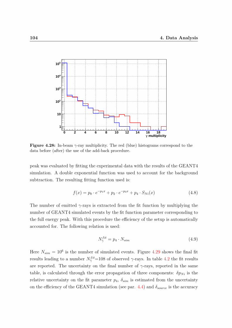
104 4. Data Analysis
multiplicityγ0 2 4 6 8 10 12 14 16 18
1
10
210
310
410
510
Figure 4.28: In-beam γ-ray multiplicity. The red (blue) histograms correspond to thedata before (after) the use of the add-back procedure.
peak was evaluated by fitting the experimental data with the results of the GEANT4simulation. A double exponential function was used to account for the backgroundsubtraction. The resulting fitting function used is:
f(x) = p0 · e−p1x + p2 · e−p3x + p4 · SNi(x) (4.8)
The number of emitted γ-rays is extracted from the fit function by multiplying thenumber of GEANT4 simulated events by the fit function parameter corresponding tothe full energy peak. With this procedure the efficiency of the setup is automaticallyaccounted for. The following relation is used:
N fitγ = p4 ·Nsim (4.9)
Here Nsim = 106 is the number of simulated events. Figure 4.29 shows the final fitresults leading to a number N fit
γ =108 of observed γ-rays. In table 4.2 the fit resultsare reported. The uncertainty on the final number of γ-rays, reported in the sametable, is calculated through the error propagation of three components: δpNi is therelative uncertainty on the fit parameter p4, δsim is estimated from the uncertaintyon the efficiency of the GEANT4 simulation (see par. 4.4) and δsource is the accuracy

4.7 Excitation Cross Section 105
on the calibration source activity.
Energy (keV)0 500 1000 1500 2000 2500 3000
cou
nts
/ 40
keV
0
5
10
15
20
25
30
35
Figure 4.29: Final 74Ni γ-ray spectrum. The blue line represents the results of theGEANT4 simulation fit.
pNi4 δpNi
4 δsim δsource N fitγ δN fit
γ
1.08 · 10−4 0.23 0.10 0.03 108 0.25
Table 4.2: Fit results and relative errors for the integral of the 1024 keV full-energypeak for the 74Ni first excited state.
4.7 Excitation Cross SectionIn order to calculate the excitation cross section, according to equation (4.1), it is
necessary to correct the measured Nmeasγ and Nmeas
B considering the live-time of theacquisition system and this is strongly related to the triggers used in the experiment.As explained in the previous chapter, the particle trigger request is given by thee1 scintillator at the focal plane of the S800. For the γ-ray part (CAESAR), themain trigger is the global OR of the 192 Constant Fraction Discriminators. As aconsequence, three different triggers can be considered:

106 4. Data Analysis
1. Particle trigger: S800 Singles;
2. Particle/γ coincidence: Coincidence = (S800 Singles) AND (CAESAR OR).
3. γ-ray single trigger: CAESAR OR;
Due to the high count rate at the focal plane of the S800, the first trigger has beendownscaled by a factor 3. Trigger requests are recorded on an event by event basis inthe data stream and can be recovered in a ”bit pattern“ format. Figure 4.30 showsthe integral values for the all measurement runs used in the analysis. The numericalvalues of the integrals are reported in table 4.3.
trigger number 1 2 3 4
nu
mb
er o
f ev
ents
510
610
710
Figure 4.30: Trigger bit pattern summed over the whole measurement data set. Trigger1 counts the S800 singles, trigger 2 the γ-ray/particle coincidences while trigger 3 consid-ers the γ-ray singles.
The bit pattern is affected by the same dead time as the acquired data. Scalersare used to measure the real number of trigger requests sent by the three differentchannels. This device has to be considered a counter not affected by dead time: the

4.7 Excitation Cross Section 107
Trigger Downscaling Bit pattern integral (BI)Particle trigger 3 14,563,797Coincidence trigger - 72,054γ-ray singles - 38,365
Table 4.3: Trigger bit integrals summed over all the statistics.
content of the scaler channels are read out and reset every 2 seconds and the dataare recorded in the event file. The channels used for the dead time estimation are:
1. Raw.Clock: samples a 10 kHz frequency oscillator. Should give a good estima-tion of the real acquisition time;
2. Live.Clock: as Raw.Clock but vetoed by the global acquisition veto;
3. S800.Source: counts the raw number of S800 triggers (not downscaled);
4. S800.Trigger: as S800.Trigger but after the downscaling;
5. Coinc.Trigger: counts the number of coincidences between S800.Trigger and theCAESAR OR;
Trigger Scaler IntegralRaw.Clock 3,473,904,072Live.Clock 3,341,247,767S800.Source 43,567,541S800.Trigger 14,521,791Coinc.Trigger 114,434
Table 4.4: Scalers integral values for the complete statistics.
The numerical values of the scalers integrals are reported in table 4.4.If we indicate as BIx the Bit-pattern Integral for channel x and as SIx the ScalerIntegral for the same channel, the live-time correction for the γ-ray integral can becomputed as follows:
LTcoinc =BIγ−raysingles +BICoincidence
SICoinc.Trigger
(4.10)

108 4. Data Analysis
Since no downscaling has been applied to this trigger the value has to be consistentwith the global live-time computed as:
LTacq =SILive.Clock
SIRaw.Clock
(4.11)
The Live-Time for particles counting in the S800 can be calculated only taking intoaccount the downscaling factor, namely:
LTS800 =BIS800singlesSIS800.Source
(4.12)
A cross check of the downscaling factor value (DSS800) can be obtained from:
DSS800 =SIS800.SourceSIS800.T rigger
(4.13)
At this point one can correct the measured values and obtain the final number offragments:
NB =Nmeas
B DSS800
ϵS800LTS800
(4.14)
Where the efficiency of the particle detectors (ϵS800) is 1. The corrected number ofγ-rays is:
Nγ =Nmeas
γ
ϵcoincLTcoinc
(4.15)
Given the Avogadro constant NA = 6.022×10²³ mol−1, the areal density of the tar-get (ρ = 642 mg/cm2) and the atomic mass of the target nuclei (A = 196.9665g/mol),NT is given by:
NT =NA ρ
A(4.16)
NB (34.8± 0.1) · 104
Nγ0+→2+ 108± 27
NT (1.94± 0.01) · 1021
Table 4.5: Summary of the values used for the cross section calculation.

4.7 Excitation Cross Section 109
Measured values are reported in table 4.5, the result for the experimental crosssection is σ0+→2+ = (159± 40) mbarn.

110 4. Data Analysis

5Results and conclusion
The B(E2; 0+ → 2+) value for the transition from the ground state to the first ex-cited state of the 74Ni nucleus can be calculated using the experimental cross sectionobtained in the previous chapter. Given the linear relationship connecting the exci-tation cross sections to the B(Eλ) values (see eq. 2.32), the results of the DWEIKOcalculation illustrated in paragraph 2.5 are linearly scaled to extract the experimentalB(E2). The result is:
B(E2; 0+ → 2+) = (694± 173) e2fm4
The obtained value is affected by an uncertainty of 25% that is mainly due to thelimit in the γ-ray peak statistics and the presence of a huge atomic background. Con-cerning the statistics, the main limiting factors is the low intensity of the produced74Ni radioactive beam that will be overcome only by the new generation radioactiveion beams facilities. The weight on the peak error of the atomic background closeto the transition peak has been estimated varying the fit parameters and consideringthe maximum peak integral variation in the two extreme cases of under and overes-

112 5. Results and conclusion
timation of the background. The difference between these two values has been usedas a more conservative error estimation with respect to what could be obtained usingthe fit errors from the minimization procedure.Figure 5.1 shows the present result for the 74Ni nucleus as well as several theoreticalexpectations and the evaluated data for the neutron rich side of the Ni isotopic chain.It has to be noticed that the this work provides the most exotic probe for the shellmodel calculations in this region since no data are available yet for N = 48 or higher.From the theoretical point of view this region has been widely studied using differentinteractions like the GXPF1A, the JUN45 (see [57] and references therein) and theCD-Bonn interaction (see [127]). The valence space covers typically the fpg shellsusing a 40Ca inert core.The recent results by L. Coraggio and collaborators [128] (violet lines of figure 5.1)clearly show the importance of the model space definition. Using a fixed interac-tion (CD-Bonn), the calculation has been performed limiting the model space to theneutron g9/2 orbital or extending it to the d5/2. The better agreement of the latter re-sults with the experimental ones clearly indicates the importance of the extension ofthe model space when increasing the neutron number along the isotopic chain. Thehigher degree of collectivity observed using a larger model space can be explainedas a consequence of allowing E2 transitions from the d5/2 to the g9/2 orbital whichcontribute to the total excitation strength.From the interaction point of view, the GXPF1A and JUN45 interactions representthe state of the art for shell model calculations. The values reported by Pritychenkoin [57] (red and dark-green curves of figure 5.1) were obtained in a reduced valencespace, namely the pf shells for GXPF1A interaction extended up to g9/2 orbital forthe JUN45. The most straight forward evolution of these results is represented bythe Monte Carlo Shell Model Calculation performed by N. Shimizu and co-workersin [129] (black line of figure 5.1). The interaction used is based on a connection be-tween the GXPF1A and the JUN45 forming the so-called A3DA interaction that hasbeen properly tuned and used within the Monte Carlo Shell Model approach. Theobtained results are in good agreement with respect to the calculations performedfor the lighter Ni isotopes and compatible with the result of the present work. Theuse of Monte Carlo Shell Model allows to overcome the limitation imposed by thedimension of the valence space allowing to span a wide range of masses (A = 56 -

113
A54 56 58 60 62 64 66 68 70 72 74 76 78
4fm2
- e
↑B
(E2)
0
200
400
600
800
1000
1200
1400
1600
1800
2000 Evaluated
GXPF1A
JUN45
This Work
Coraggio - g9/2 [128]
Coraggio - d5/2 [128]
Shimizu [129]
Sieja [130]
Figure 5.1: Experimental values and theoretical expectations for the B(E2 ↑) matrixelement of the known even-even Ni isotopes. Data are from [57, 128–130], complementedwith the result of the present analysis.
A = 78). It is worth to notice that the model by N. Shimizu and co-workers pre-dicts an increase of the B(E2) value for the 78Ni nucleus, opposite to what one couldexpect given the nominal double shell closure at Z = 28 and N = 50. This featureis very interesting and it underlines the importance of a better determination of theingredients needed to describe the structure in this exotic mass region. With respectto our result, the most compatible B(E2) value is the one calculated by Sieja andNowacki in [130] (green line of figure 5.1) who performed Large Scale Shell Model cal-culations. In this case the starting point for the two-body matrix elements definitionis the previous work performed in the A = 70 neutron rich nuclear region where thephenomena of a new island of inversion was studied (see [131]). The interaction wasproperly adapted to constrain the gap evolution from 68Ni to 78Ni without affectingthe structure of the island of inversion (see fig. 5.2). This phenomenon consists inthe non-standard reordering of the nuclear shells due to the deformation induced bystrong quadrupole correlations able overcome the spherical mean-field gaps. In thissituation deformed intruders can be energetically favored and often become nuclearground states. Figure 5.2 shows the evolution of single particle energies (monopoleterm of the interaction) for the N = 50 isotones (left panel) and for the most neu-tron rich Ni isotopes. The good agreement of the present result with the result ofthis calculation using the modified monopole term underlines the importance of the

114 5. Results and conclusion
-20
-15
-10
-5
0
5
28 34 38
ES
PE
(MeV
)
Proton number
f5/2p3/2p1/2g9/2d5/2
-25
-20
-15
-10
-5
0
5
40 50
ES
PE
(MeV
)Neutron number
f7/2p3/2f5/2p1/2g9/2d5/2
Figure 5.2: Left panel: Evolution of the neutron effective single particle energies withthe proton number at N = 50. Right panel: Evolution of the neutron effective singleparticle energies for the Ni isotopes (in the range N = 40-N = 50). Adapted from [130].
evolution of the single particle energies for nuclei with large neutron excess.
Concerning the experimental data shown in figure 5.1 as evaluated by Pritychenkoand co-workers, it is important to recall that the only experimental information avail-able on the 74Ni nucleus is the one obtained by Aoi and collaborators in [72]. Themeasured value is quite different from the one obtained in this work but it has to beunderlined that the two results have been derived using different techniques. By def-inition, the Coulomb excitation mechanism is only sensitive to the electromagneticinteraction between the reaction partners (nuclear interactions contributions havebeen explicitly removed by a cut on the impact parameter), while Aoi and co-workersperformed a proton scattering experiment where both the nuclear and Coulomb in-teractions act in the excitation process. If this difference is confirmed, there couldbe the indication of an important de-coupling of the neutron and proton shells inpresence of a strong neutron excess that could lead to different proto/neutron coresdeformation. It is clear that other new measurements in the same mass region arestill needed to confirm and complete the present study: further proton scattering andCoulomb excitation experiments using the nuclei surrounding 74Ni will give more in-formation about this exotic region of the nuclear chart. As an example, the 72Niproton scattering experiment is planned in June 2013 at MSU.More generally speaking, the present result underlines once more the importance ofthe new generation facilities that will provide more intense and more exotic radioac-

115
tive ion beams, allowing for a more complete and precise study of the evolution ofthe nuclear shells .

116 5. Results and conclusion

Bibliography
[1] G. F. Bertsch, D. J. Dean, and W. Nazarewicz, Scidac review: Subatomic dis-covery through advanced computing, http://www.scidacreview.org/0704/html/unedf.html.
[2] D. Bazin, Nature 486, 330 (2012).
[3] J. Al-Khalili, An introduction to halo nuclei, in The Euroschool Lectures onPhysics with Exotic Beams, Vol. I, edited by J. Al-Khalili and E. Roeckl, volume651 of Lecture Notes in Physics, pp. 77–112, Springer Berlin Heidelberg, 2004.
[4] G. Audi, A. Wapstra, and C. Thibault, Nuclear Physics A 729, 337 (2003).
[5] T. Otsuka, T. Matsuo, and D. Abe, Phys. Rev. Lett. 97, 162501 (2006).
[6] D. Shetty and S. Yennello, arXiv:1002.0313v4 [nucl-ex] (2010).
[7] M. Baldo, Nuclear Methods and the Nuclear Equation of State (World Scientific,1999).
[8] National nuclear data center, http://www.nndc.bnl.gov/.
[9] J. Al-Khalili and E. Roeckl, The Euroschool Lectures on Physics with ExoticBeams, Lecture Notes in Physics No. v. 3 (Springer, 2008).
[10] M. G. Mayer, Phys. Rev. 75, 1969 (1949).
[11] O. Haxel, J. H. D. Jensen, and H. E. Suess, Phys. Rev. 75, 1766 (1949).
[12] E. Gadioli and I. Università degli studi (Milan, Proceedings of the 11th Inter-national Conference on Nuclear Reaction Mechanisms: Varenna, June 12-16,2006 (Universita degli studi di Milano, 2006).
[13] J. Dobaczewski, I. Hamamoto, W. Nazarewicz, and J. A. Sheikh, Phys. Rev.Lett. 72, 981 (1994).
[14] Website, The EURISOL design study, http://www.eurisol.org/site02/index.php.

118 BIBLIOGRAPHY
[15] T. Otsuka and A. Schwenk, Nuclear Physics News International 22, 12 (2012).
[16] T. Otsuka et al., Phys. Rev. Lett. 104, 012501 (2010).
[17] T. Otsuka, T. Suzuki, R. Fujimoto, H. Grawe, and Y. Akaishi, Phys. Rev. Lett.95, 232502 (2005).
[18] T. Otsuka, M. Honma, and D. Abe, Nuclear Physics A 788, 3 (2007).
[19] M. Honma, T. Otsuka, B. A. Brown, and T. Mizusaki, Phys. Rev. C 69, 034335(2004).
[20] T. Otsuka, T. Suzuki, J. D. Holt, A. Schwenk, and Y. Akaishi, Phys. Rev.Lett. 105, 032501 (2010).
[21] G. Hagen, M. Hjorth-Jensen, G. R. Jansen, R. Machleidt, and T. Papenbrock,Phys. Rev. Lett. 109, 032502 (2012).
[22] H. Grawe et al., The European Physical Journal A - Hadrons and Nuclei 25,357 (2005).
[23] B. Brown, (2005).
[24] H. Grawe, Acta Physica Polonica B 34, 2267–2275 (2003).
[25] H. Grawe and M. Lewitowicz, Nuclear Physics A 693, 116 (2001).
[26] A. Gadea et al., Eur. Phys. J. A 20, 193 (2004).
[27] A. Stefanini et al., Nuclear Physics A 701, 217 (2002), 5th InternationalConference on Radioactive Nuclear Beams.
[28] E. Farnea and D. Bazzacco, Nuclear Physics News International 22, 27 (2012).
[29] D. Scarpa et al., European Physical Journal A 47 (2011).
[30] Website, EURISOL design study, task 3: direct target, http://www.eurisol.org/site02/direct_target/.
[31] Website, The ISOLDE facility at CERN, http://isolde.web.cern.ch/isolde/.
[32] Website, ISAC Facilities for Rare-Isotope Beams,http://www.triumf.ca/research/research-facilities/isac-facilities-for-rare-isotope-beams.
[33] Website, HRIBF Facilities for Rare-Isotope Beams (ORNL), http://www.phy.ornl.gov/hribf/.

BIBLIOGRAPHY 119
[34] Website, GANIL - SPIRAL II facility, http://www.ganil-spiral2.eu/.
[35] Website, SPES - Selective Ions For Exotic Species, http://web.infn.it/spes/.
[36] A. Andrighetto et al., NUCLEAR PHYSICS A 834, 754C (2010).
[37] T. Baumann, A. Amthor, D. Bazin, and B. A. Brown, Nature 449, 1022 (2007).
[38] Website, GANIL - SPIRAL In Flight facility, http://www.ganil-spiral2.eu/science-us/accelerator/spiral.
[39] Website, The GSI Fragment Separator, http://www-wnt.gsi.de/frs/index.asp.
[40] Website, RIKEN NiSHiNa center for Accelerator-based science, http://www.nishina.riken.jp/Eng/.
[41] Website, NSCL A1900 fragment separator, http://www.nscl.msu.edu/tech/devices/a1900.
[42] Website, FRIB - Facility for Rare Isotope Beams, http://www.frib.msu.edu/.
[43] Website, FAIR - An International Facility for Antiproton and Ion Research,http://www.fair-center.eu/.
[44] Website, GSI Helmholtzzentrum für Schwerionenforschung, http://www.gsi.de/.
[45] Website, The CAlifornium Rare Isotope Breeder Upgrade (CARIBU) (ANL),http://www.phy.anl.gov/atlas/caribu/index.html.
[46] G. Tabacaru et al., REVIEW OF SCIENTIFIC INSTRUMENTS 83 (2012).
[47] Website, The EXCYT radioactive beam facility (INFN - LNS), http://www.lns.infn.it/excyt/index.html.
[48] Website, Inter University Accelerator Centre - Heavy Ion Reaction Analyzer,New Delhi, http://www.iuac.res.in/refac/np/hira/hira_main.html.
[49] Website, Variable Energy Cyclotron Centre - Kolkata, http://www.vecc.gov.in/.
[50] http://ie.lbl.gov/systematics/chart2000g.pdf.
[51] B. Blank et al., Phys. Rev. Lett. 84, 1116 (2000).
[52] C. Dossat et al., Phys. Rev. C 72, 054315 (2005).
120 BIBLIOGRAPHY
[53] C. Engelmann et al., Zeitschrift für Physik A Hadrons and Nuclei 352, 351(1995).
[54] P. T. Hosmer et al., Phys. Rev. Lett. 94, 112501 (2005).
[55] T. Ohnishi et al., Journal of the Physical Society of Japan 79, 073201 (2010).
[56] O. Sorlin and M.-G. Porquet, Progress in Particle and Nuclear Physics 61, 602(2008).
[57] B. Pritychenko, J. Choquette, M. Horoi, B. Karamy, and B. Singh, AtomicData and Nuclear Data Tables 98, 798 (2012).
[58] O. Kenn et al., Phys. Rev. C 63, 064306 (2001).
[59] T. Ishii et al., Phys. Rev. Lett. 84, 39 (2000).
[60] H. Grawe, M. Górska, and J. Döring, AIP Conf. Proc. 561, 287 (2000).
[61] A. Oros-Peusquens and P. Mantica, Nuclear Physics A 669, 81 (2000).
[62] O. Sorlin et al., Phys. Rev. Lett. 88, 092501 (2002).
[63] M. Sawicka et al., Phys. Rev. C 68, 044304 (2003).
[64] K. Langanke, J. Terasaki, F. Nowacki, D. J. Dean, and W. Nazarewicz, Phys.Rev. C 67, 044314 (2003).
[65] C. Mazzocchi et al., Physics Letters B 622, 45 (2005).
[66] O. Perru et al., Phys. Rev. Lett. 96, 232501 (2006).
[67] K. L. Yurkewicz et al., Phys. Rev. C 70, 054319 (2004).
[68] A. Bohr, R. Broglia, and S. italiana di fisica, Elementary modes of excitationin nuclei:Proceedings of the International School of Physics ”Enrico Fermi”(North-Holland Pub. Co., 1977).
[69] R. Casten, Nuclear Structure from a Simple PerspectiveOxford Studies in Nu-clear Physics (Oxford University Press, 2000).
[70] G. Kraus et al., Phys. Rev. Lett. 73, 1773 (1994).
[71] T. Otsuka, M. Honma, and T. Mizusaki, Phys. Rev. Lett. 81, 1588 (1998).
[72] N. Aoi et al., Physics Letters B 692, 302 (2010).
[73] S. Franchoo et al., Phys. Rev. C 64, 054308 (2001).

BIBLIOGRAPHY 121
[74] W. Hamilton, The Electromagnetic interaction in nuclear spectroscopy (North-Holland, 1975).
[75] K. Krane and D. Halliday, Introductory nuclear physics (Wiley, 1987).
[76] R. Bass, Nuclear Reactions with Heavy IonsTexts and monographs in physics(Springer, 1980).
[77] J. Jackson, Classical Electrodynamics (Wiley, 1998).
[78] C. Bertulani, arXiv (2009), 0908.4307.
[79] K. Alder, A. Bohr, T. Huus, B. Mottelson, and A. Winther, Rev. Mod. Phys.28, 432 (1956).
[80] K. Alder and A. Winther, Electromagnetic excitation: theory of Coulomb exci-tation with heavy ions (North-Holland Pub. Co., 1975).
[81] A. Winther and K. Alder, Nuclear Physics A 319, 518 (1979).
[82] C. Bertulani and G. Baur, Nuclear Physics A 442, 739 (1985).
[83] C. A. Bertulani and G. Baur, Physics Reports 163, 299 (1988).
[84] C. von Weizsacker, Z.Phys. 88, 612 (1934).
[85] E. J. Williams, Phys. Rev. 45, 729 (1934).
[86] B. Hoffmann and G. Baur, Phys. Rev. C 30, 247 (1984).
[87] A. Goldberg, Nuclear Physics A 420, 636 (1984).
[88] C. A. Bertulani and G. Baur, Phys. Rev. C 33, 910 (1986).
[89] G. Baur, C. Bertulani, and H. Rebel, Nuclear Physics A 458, 188 (1986).
[90] A. Aleixo and C. Bertulani, Nuclear Physics A 505, 448 (1989).
[91] T. Glasmacher, Nuclear Physics A 693, 90 (2001).
[92] C. Bertulani, Computer Physics Communications 116, 345 (1999).
[93] W. Wilcke et al., Atomic Data and Nuclear Data Tables 25, 389 (1980).
[94] F. Delaunay and F. Nunes, J.Phys. G34, 2207 (2007), 0708.3007.
[95] J. M. Cook, T. Glasmacher, and A. Gade, Phys. Rev. C 73, 024315 (2006).
[96] S. RAMAN, C. N. JR., and P. TIKKANEN, Atomic Data and Nuclear DataTables 78, 1 (2001).

122 BIBLIOGRAPHY
[97] C. Bertulani, G. Cardella, M. D. Napoli, G. Raciti, and E. Rapisarda, PhysicsLetters B 650, 233 (2007).
[98] H. Scheit, A. Gade, T. Glasmacher, and T. Motobayashi, Physics Letters B659, 515 (2008).
[99] C. Bertulani, C. Campbell, and T. Glasmacher, Computer Physics Communi-cations 152, 317 (2003).
[100] D. Weisshaar, Private communication .
[101] P. Závodszky et al., Proceedings of Cyclotrons and Their Applications 2007,Eighteenth International Conference .
[102] L. Sun et al., Proceedings of ECRIS2010, Grenoble, France .
[103] X. Wu, H. Blosser, D. Johnson, F. Marti, and R. York, Proceedings of the 1999Particle Accelerator Conference, New York, 1999 .
[104] LISE++ computer code, http://lise.nscl.msu.edu/lise.html.
[105] K. Sümmerer and B. Blank, Phys. Rev. C 61, 034607 (2000).
[106] A. Stolz et al., Nuclear Instruments and Methods in Physics Research SectionB: Beam Interactions with Materials and Atoms 241, 858 (2005).
[107] D. Morrissey, B. Sherrill, M. Steiner, A. Stolz, and I. Wiedenhoever, NuclearInstruments and Methods in Physics Research Section B: Beam Interactionswith Materials and Atoms 204, 90 (2003).
[108] B. Sherrill, D. Morrissey, J. N. Jr., and J. Winger, Nuclear Instruments andMethods in Physics Research Section B: Beam Interactions with Materials andAtoms 56–57, Part 2, 1106 (1991).
[109] D. Bazin, J. Caggiano, B. Sherrill, J. Yurkon, and A. Zeller, Nuclear Instru-ments and Methods in Physics Research Section B: Beam Interactions withMaterials and Atoms 204, 629 (2003).
[110] S800 spectrograph inverse map server.
[111] D. Bazin, S800 service level destription, nscl internal document.
[112] J. Yurkon et al., Nuclear Instruments and Methods in Physics Research SectionA: Accelerators, Spectrometers, Detectors and Associated Equipment 422, 291(1999).
[113] M. Berz, K. Joh, J. A. Nolen, B. M. Sherrill, and A. F. Zeller, Phys. Rev. C47, 537 (1993).

BIBLIOGRAPHY 123
[114] D. Weisshaar et al., Nuclear Instruments and Methods in Physics ResearchSection A: Accelerators, Spectrometers, Detectors and Associated Equipment624, 615 (2010).
[115] S. Akkoyun et al., Nuclear Instruments and Methods in Physics ResearchSection A: Accelerators, Spectrometers, Detectors and Associated Equipment668, 26 (2012).
[116] S. Paschalis et al., Nuclear Instruments and Methods in Physics ResearchSection A: Accelerators, Spectrometers, Detectors and Associated Equipment ,(2013).
[117] T. L. website, http://teledynelecroy.com/lrs/dsheets/4300b.htm.
[118] G. Knoll, Radiation detection and measurement (Wiley, 2000).
[119] W. Leo, Techniques for Nuclear and Particle Physics Experiments: A How-ToApproach (Springer, 1994).
[120] S. Ahmed, Physics and Engineering of Radiation Detection (Elsevier Science,2007).
[121] T. Baugher, to be published .
[122] R. Brun and F. Rademakers, Nuclear Instruments and Methods in Physics Re-search Section A: Accelerators, Spectrometers, Detectors and Associated Equip-ment 389, 81 (1997).
[123] K. Wimmer, NSCL S800 ROOT data analysis software, http://www.nscl.msu.edu/~wimmer.
[124] K. Wimmer, NSCL S800 ROOT data analysis software user manual, http://www.nscl.msu.edu/~wimmer/manual/NSCL_ROOT_usermanual.pdf.
[125] S. Agostinelli et al., Nuclear Instruments and Methods in Physics ResearchSection A: Accelerators, Spectrometers, Detectors and Associated Equipment506, 250 (2003).
[126] A. Estrade, Time-Of-Flight Mass Measurements of Neutron Rich Isotopes atthe NSCL. (PhD thesis, 2010).
[127] R. Machleidt, Phys. Rev. C 63, 024001 (2001).
[128] L. Coraggio, Private communication .
[129] N. Shimizu et al., Progress of Theoretical and Experimental Physics 2012(2012).

124 BIBLIOGRAPHY
[130] K. Sieja and F. Nowacki, arXiv:1201.0373 [nucl-th] (2012).
[131] S. M. Lenzi, F. Nowacki, A. Poves, and K. Sieja, Phys. Rev. C 82, 054301(2010).

Acknowledgments
The last three years have certainly been one the most intense periods of my life.
Having the possibility to complement the PhD school studies with an intense research
activity at the Legnaro National Laboratory (INFN), I had the opportunity to grow
and learn in one of the most lively scientific frameworks that the Italian research
can offer. For this I have to thank my supervisor, prof. Giovanna Montagnoli, who
followed my PhD with care and interest and let me free to pursue my research cu-
riosity. I also would like to thank my co-supervisor dr. Giacomo De Angelis, who is
the ”father“ of the experiment presented in this thesis, for allowing me to work on
this data analysis and for introducing me into the world of nuclear spectroscopy with
useful teachings and suggestions.
A special thank to dr. Fabiana Gramegna that, apart from co-supervising this work,
is my tutor in several activities since almost five years. She is the driving force of my
scientific growth and I will never thank her enough for what she has been doing for
me.
The experiment described in this work was performed at NSCL and it would have
never been possible without the support of the local group. Among the others, I
would like to thank prof. Alexandra Gade and dr. Dirk Weisshaar for the precious
contribution to the experiment and for their suggestions during the data analysis
and dr. Trevis Baugher who provided the simulation code. I’m really grateful to
dr. Kathrin Wimmer for her continuous support during the data analysis and for

126 BIBLIOGRAPHY
providing an important part of the code I used.
This thesis would not have been written without the priceless help of dr. Enrico
Farnea. Thanks for your help in the difficult task of writing and finalizing the anal-
ysis and for being the fastest and most efficient proofreader that I’ve ever seen!
I’d like also to thank the people of the LNL-PD INFN gamma group for several
fruitful discussions and suggestions for the analysis. Among the others dr. Caterina
Michelagnoli, dr. Andrea Gottardo and dr. José Javier Valiente Dobón.
Since my three-year thesis in 2006 I’ve been part of the NUCL-EX collaboration and
I was involved in several activities at LNL. It is impossible to summarize in few words
the incredible amount of experiences, shifts, and the hard work we did together... I’ll
simply say a big THANK YOU! to everyone.
A special thank to Caterina and Enrico, good friends and the best uncles ever. We
spent very good times together, very crazy times also... but this makes life more
interesting!
Finally I would like to dedicate this work to Daniela and Benedetta: whenever,
wherever with you I feel at home.