arX

iv:1

410.

8644

v1 [

nucl

-th]

31

Oct

201

4

Continuum quasiparticle random phase approximation for

astrophysical direct neutron capture reaction of neutron-rich

nuclei

Masayuki Matsuo

Department of Physics, Faculty of Science,

Niigata University, Niigata 950-2181, Japan

(Dated: July 10, 2018)

Abstract

We formulate a many-body theory to calculate the cross section of direct radiative neutron capture

reaction by means of the Hartree-Fock-Bogoliubov mean-field model and the continuum quasiparticle

random phase approximation (QRPA). A focus is put on very neutron-rich nuclei and low-energy

neutron kinetic energy in the range of O(1 keV) - O(1 MeV), relevant for the rapid neutron-capture

process of nucleosynthesis. We begin with the photo-absorption cross section and the E1 strength

function, then, in order to apply the reciprocity theorem, we decompose the cross section into

partial cross sections corresponding to different channels of one- and two-neutron emission decays

of photo-excited states. Numerical example is shown for the photo-absorption of 142Sn and the

neutron capture of 141Sn.

PACS numbers: 21.60.Jz 25.20.Dc 25.60.Tv 26.30.Hj

1

I. INTRODUCTION

The radiative neutron capture, i.e. (n, γ) reaction, is one of the fundamental nuclear

reactions essential in various nucleosynthesis models. In the rapid neutron-capture process

(r-process), relevant to the origin of heavy elements, the reaction takes place in short-lived

neutron-rich nuclei, for which direct experimental measurement of the neutron capture cross

section is practically impossible. Naturally, an alternative method to measure the inverse

reaction, e.g. the Coulomb dissociation, has been considered, but the actual application is

quite limited at present even though the experimental possibilities increase with the advances

of the RI beam facilities, see for example [1, 2].

The neutron capture reaction is often classified into two different processes depending on

the neutron separation energy or the excitation energy after the capture (see, e.g., [3] as a

review). One is the compound process in which formation of compound states after absorption

of a neutron is assumed, and statistical models are often employed. The compound process

has been adopted to describe the slow and rapid neutron-capture processes which take place

in stable nuclei or unstable nuclei with large neutron separation energy sufficient to give

excitation energy to form the compound states. The main building blocks of the model is

the neutron transmission coefficient for the formation of compound states and the gamma-

decay strength function for the statistical gamma decay. Recently new modes of dipole

excitation such as the pygmy resonance and the soft dipole excitation[4–7] have attracted

attentions since influence of the new modes on the r-process nucleosynthesis was pointed

out [8]. Motivated with this possibility, microscopic many-body models of electric multipole

responses, developed on the basis of the density functional theories, have been applied to the

gamma-ray strength function for the compound process calculations [9–14].

The other is the direct radiative capture process in which a electromagnetic transition is

assumed to take place from an initial state including the incoming neutron to bound final

states without forming compound states. It is estimated that the r-process nucleosynthesis

in very neutron-rich nuclei is dominated by the direct process since the formation of the

compound states is not likely in neutron-rich nuclei due to small neutron separation energy

and small level density at the threshold[3, 15, 16]. Direct neutron capture calculations[15–23]

often assumes a simple potential picture in which the initial and final states are described

2

as scattering and bound single-particle states. However, one can expect that the new dipole

excitation modes may affect the direct neutron capture process likewise in the case of the

compound process. To unveil the effect it is necessary to construct a many-body theory of the

direct neutron capture reaction in which the correlations in multipole modes of excitation

are taken into account. It is the purpose of the present paper to demonstrate that the

quasiparticle random phase approximation provides such a framework.

The random phase approximation based on the density functional models has been one

of the most powerful theoretical framework to describe electromagnetic responses of nuclei,

including new modes in exotic nuclei (see, e.g., [7] as a review, and references therein).

The same is for the photo-absorption cross section. Note here that the photo-absorption

reaction may have different final reaction channels if nucleons are allowed to be emitted from

the photo-excited states. Among them, a reaction followed by one-neutron emission, i.e.,

(γ, n) reaction, is the inverse process of the relevant (n, γ) reaction. It is then possible to

evaluate the (n, γ) cross section using the reciprocity theorem, provided that one can calculate

partial cross sections associated with one-neutron emission decays. We note here a method of

Zangwill and Soven[24], which is used to describe the partial photo-absorption cross section

of atoms[24] and molecules [25] by means of the continuum RPA. In the case of neutron-

rich nuclei, however, the pair correlation plays important roles[6, 26–30], and not only one

neutron but also two neutrons can be emitted only with small excitation energy. We shall

show in the present paper that the partial photo-absorption cross sections corresponding to

individual decay channels can be calculated by applying the Zangwill-Soven method to the

continuum quasiparticle random phase approximation (cQRPA)[31–33], a version of QRPA,

in which the pair correlation is described with the Bogoliubov theory, and the continuum

states relevant to the one- and two-neutron emission are described with the proper scattering

boundary condition.

We remark that special cares are required to describe capture of a neutron with very low

kinetic energy: the energy range relevant to the r-process is En ∼ O(1 keV) -O(1 MeV),

corresponding to the temperature T ∼ O(107) - O(109) K of possible r-process environments,

and hence we need a fine energy resolution, which is not required in usual RPA or QRPA

descriptions of nuclear responses. It should be noted also that the r-process pass may reach to

nuclei close to the neutron drip-line having very small one-neutron separation energy S1n ∼ 1

3

MeV. In such a case we need wave functions of neutrons up to very large distances from the

center of the nucleus. Numerical procedures to meet these requirements are also discussed in

the present paper.

II. CONTINUUM QUASIPARTICLE RANDOM PHASE APPROXIMATION FOR

DIRECT NEUTRON CAPTURE CROSS SECTION

A. Total photo-absorption cross section in QRPA

We shall briefly recapitulate the quasiparticle random phase approximation (QRPA) and

its application to a description of the total photo-absorption cross section in order to provide

a basis for later discussion.

The photo-absorption reaction is an excitation of a nucleus caused by the electromagnetic

transition. Assuming the dominant electric dipole transition (E1 transition) and the second

order perturbation with respect to the photo-nuclear interaction, the cross section is given[34,

35] as

σγ(Eγ) =16π3e2Eγ

3hc

∑

k

| 〈k|D0 |0〉 |2δ(Eγ − hωk) (1)

with the dipole operator D0 = ZA

∑

p rpY10(rp) −NA

∑

n rnY10(rn). Here |0〉 and |k〉 are the

ground and excited states of the nucleus with the excitation energy hωk. The cross section

σγ(Eγ) is proportional to the strength function

S(hω) =∑

k

| 〈k| D0 |0〉 |2δ(hω − hωk) (2)

with Eγ = hω, multiplied with the factor f(Eγ) = 16π3e2Eγ/3hc.

The strength function is formulated by considering linear response of the system under an

external one-body field

Vext(t) = Vexte−iωt + V †

exte−iωt (3)

with Vext = D0. In QRPA, the response is described on the basis of the time-dependent

Hartree-Fock-Bogoliubov (TDHFB) theory (which may be called also the time-dependent

Kohn-Sham-Bogoliubov theory), whose basic equation is

ih∂

∂t|Φ(t)〉 = (h[R(t)] + Vext(t)) |Φ(t)〉 . (4)

4

Here |Φ(t)〉 is the time-evolving generalized determinant state and h[R(t)] = T + Vmf [R(t)]

is the TDHFB(TDKSB) self-consistent Hamiltonian defined by the variation of the energy

density functional Etot[R] = 〈Φ|T |Φ〉+Ex[R] with respect to the generalized density matrix

matrix R.

In the following we assume that the functional is written in terms of quasi-local one-body

densities. The simplest are the one-body density ρ(r) =∑

σ

⟨

Φ|ψ†(rσ)ψ†(rσ)|Φ⟩

and the

pair-density ρ(r) =⟨

Φ|ψ(rσ)ψ†(rσ)|Φ⟩

and its conjugate ρ∗(r) while it is not difficult to

take into account other quasi-local densities such as the spin, current, kinetic energy and

spin-orbit densities, utilized in the Skyrme functional models[36]. In the following, all these

quasi-local densities are denoted as

ρα(r) = 〈Φ|ρα(r)|Φ〉 (5)

with the index α distinguishing the kinds. We also use a collective notation {ρ}. Here ρα(r)

are corresponding one-body operators. ( In the following we assume that the operators satisfy

the (anti) hermiticity ρα(r)† = sαρα(r) with sα = ±1.) The TDHFB mean-field Vmf is then

expressed as

Vmf [{ρ(t)}] =∑

α

∫

drvmfα (r, t)ρα(r), (6)

in terms of the functional derivative vmfα (r, t) = ∂Ex[{ρ(t)}]/∂ρα(r). We also assume that

the external field is expressed as

Vext =∑

α

∫

drvextα (r)ρα(r). (7)

Considering the time-evolution in the linear response approximation, we describe the

fluctuating part |δΦ(t)〉 of the state vector |Φ(t)〉 around the HFB ground state |Φ0〉:

(ih∂

∂t− h0) |δΦ(t)〉 = (Vext(t) + δVind(t)) |Φ0〉 , (8)

where

δVind(t) =∑

αβ

∫

drκαβ(r)δρβ(r, t)ρα(r), (9)

is fluctuation in the TDHFB mean-field Vmf [{ρ(t)}], and is often called the induced field.

It arises from fluctuation in the densities δρα(r, t) = 〈Φ0|ρα(r)|δΦ(t)〉 + 〈δΦ(t)|ρα(r)|Φ0〉.

5

καβ(r) is the residual interaction given as the second derivatives of the functional:

καβ(r) =∂2Ex[{ρ}]

∂ρα(r)∂ρβ(r). (10)

Note that the source of |δΦ(t)〉 is not only the external field Vext(t) but also the induced

field δVind(t), as indicated by Eq.(8). Their sum is called the selfconsistent field[24, 25], which

is given in the frequency domain as

Vscf(ω) ≡ Vext + δVind(ω) =∑

α

∫

drvscfα (r, ω)ρα(r), (11)

vscfα (r, ω) = vextα (r) +∑

γ

καγ(r)δργ(r, ω). (12)

The fluctuating densities δρα(r, t) are governed in the frequency domain by the linear

response equation:

δρα(r, ω) =

∫

dr′∑

β

Rαβ0 (r, r′, ω)

(

∑

γ

κβγ(r′)δργ(r

′, ω) + vextβ (r′)

)

. (13)

Here Rαβ0 (r, r′, ω) is the unperturbed response function, which is expressed in the spectral

representation as

Rαβ0 (r, r′, ω) =

∑

i<j

[

〈0|ρα(r)|ij〉 〈ij|ρβ(r′)|0〉

hω + iǫ− Ei − Ej−

〈0|ρβ(r′)|ij〉 〈ij|ρα(r)|0〉

hω + iǫ+ Ei + Ej.

]

(14)

Here use is made of the quasiparticle states i and j, which are Fermionic elementary modes

of the static HFB Hamiltonian h0 = T + Vmf [{ρ0}], defined by [h0, a†i ] = Eia

†i . |0〉 denotes

the HFB ground state |Φ0〉, and |ij〉 ≡ a†ia†j |Φ0〉 are two-queasiparticle states.

The strength function is given in terms of the density response as

S(hω) = −1

πIm

∫

dr∑

α

vextα (r)δρα(r, ω). (15)

with vextα (r) = vextα (r)∗sα.

B. Partial cross sections for specific decay channels

After absorbing a photon, the excited nucleus may decay by emitting one or multiple nu-

cleon(s) if the excitation energy is larger than the threshold energies for the particle emissions.

6

We shall formulate here a method to evaluate partial cross sections of the photo-absorption

reaction defined for specific decay channels. To this end, we extend the method of Zangwill

and Soven[24] that is originally formulated for the continuum RPA theory neglecting the pair

correlations. We shall show here that the scheme can be generalized to the case of superfluid

nuclei by using the Bogoliubov quasiparticles instead of the single-particle states.

The starting point of the method is to note that the strength Eq.(15) is rewritten as

S(hω) = −1

πIm

∫ ∫

drdr′∑

αβ

vscfα (r, ω)Rαβ0 (r, r′, ω)vscfβ (r′, ω) (16)

in terms of the selfconsistent field and the unperturbed response function. The derivation is

given in Appendix A. Using the spectral representation for R0(ω), it is further written as

S(hω) = −1

πIm∑∑

i>j

{

| 〈ij| Vscf(ω) |0〉 |2

hω + iǫ− Ei −Ej

−| 〈0| Vscf(ω) |ij〉 |

2

hω + iǫ+ Ei + Ej

}

=∑∑

i>j

| 〈ij| Vscf(ω) |0〉 |2δǫ(hω − Eij)− | 〈0| Vscf(ω) |ij〉 |

2δǫ(hω + Eij) (17)

with a Lorentz function

δǫ(hω ∓ Eij) ≡1

π

ǫ

(hω ∓Eij)2 + ǫ2, Eij = Ei + Ej. (18)

We here recall (see Eq.(8)) that the time-dependent field causing evolution of the system

includes not only the external field Vext(t) = Vexte−iωt + V †

exteiωt but also the induced field

δVind(t). This points to that 〈ij| Vscf(ω) |0〉 is the matrix element for transition from the

ground state |0〉 to a two-quasiparticle state |ij〉. If we take the limit ǫ → 0 in which δǫ(E)

converges to the delta function δ(E), then we may interpret that each term of Eq.(17) is

proportional to

wij =2π

h| 〈ij| Vscf(ω) |0〉 |

2δ(hω − Eij), (19)

which represents the transition probability per unit time from the the HFB ground state |0〉

to a two-quasiparticle state |ij〉. However, we need to pay attentions to spectral properties

of the quasiparticle and two-quasiparticle states in order to give precise interpretations to

individual terms.

The quasiparticle eigenstates of the HFB Hamiltonian h0 are categorized as either discrete

bound states or continuum unbound states[26, 27]. The discrete bound states are states

7

satisfying Ei < |λ| with λ being the Fermi energy, and they correspond to bound single-

particle orbits which are located around the Fermi energy. We label them with m,n etc.

in the following. Those with Ei > |λ| are all unbound states belonging to a continuum

spectrum, and they describe a scattering nucleon. For the continuum quasiparticle states we

use labels p(Ep), q(Eq) etc. with explicit quasiparticle energy. Note that a part of single-

particle hole orbits is embedded in the continuum spectrum due to the coupling caused by

the pair potential. Such hole-like quasiparticle states are resonances in the HFB model.

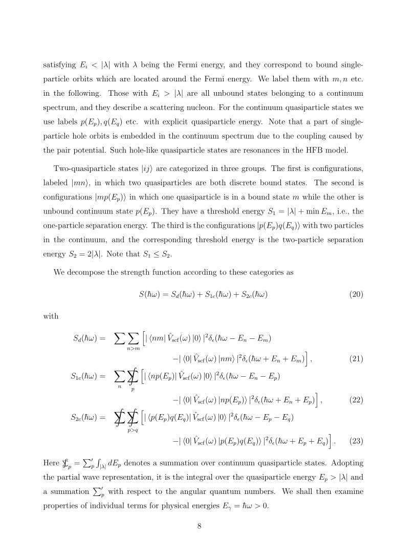
Two-quasiparticle states |ij〉 are categorized in three groups. The first is configurations,

labeled |mn〉, in which two quasiparticles are both discrete bound states. The second is

configurations |mp(Ep)〉 in which one quasiparticle is in a bound state m while the other is

unbound continuum state p(Ep). They have a threshold energy S1 = |λ|+minEm, i.e., the

one-particle separation energy. The third is the configurations |p(Ep)q(Eq)〉 with two particles

in the continuum, and the corresponding threshold energy is the two-particle separation

energy S2 = 2|λ|. Note that S1 ≤ S2.

We decompose the strength function according to these categories as

S(hω) = Sd(hω) + S1c(hω) + S2c(hω) (20)

with

Sd(hω) =∑∑

n>m

[

| 〈nm| Vscf(ω) |0〉 |2δǫ(hω − En − Em)

−| 〈0| Vscf(ω) |nm〉 |2δǫ(hω + En + Em)]

, (21)

S1c(hω) =∑

n

∑

∫

p

[

| 〈np(Ep)| Vscf(ω) |0〉 |2δǫ(hω − En − Ep)

−| 〈0| Vscf(ω) |np(Ep)〉 |2δǫ(hω + En + Ep)

]

, (22)

S2c(hω) =∑

∫

∑

∫

p>q

[

| 〈p(Ep)q(Eq)| Vscf(ω) |0〉 |2δǫ(hω − Ep −Eq)

−| 〈0| Vscf(ω) |p(Ep)q(Eq)〉 |2δǫ(hω + Ep + Eq)

]

. (23)

Here∑

∫

p=∑′

p

∫

|λ|dEp denotes a summation over continuum quasiparticle states. Adopting

the partial wave representation, it is the integral over the quasiparticle energy Ep > |λ| and

a summation∑′

p with respect to the angular quantum numbers. We shall then examine

properties of individual terms for physical energies Eγ = hω > 0.

8

Let us first consider S1c(hω) which collects contributions of two-quasiparticle configura-

tions {|np(Ep)〉}. These configurations consist of one quasiparticle in a scattering state p(Ep)

and the remaining odd-A nucleus in a one-quasiparticle state |n〉 = a†n |0〉. Now consider exci-

tation energy hω > En+ |λ| larger than the threshold of this configuration. Then the integral

range of∫

|λ|dEp includes the peak Ep = hω − En of the Lorentz function δǫ(hω − En − Ep)

and hence δǫ(hω − En − Ep) can be treated as the delta function while δǫ(hω + En + Ep)

gives a contribution vanishing in the limit ǫ → 0. Therefore we find that each summand of

S1c(hω) in Eq.(22) represents the probability of populating the one-quasiparticle state |n〉

and one particle emitted in the continuum scattering state p(Ep). With multiplication of the

kinematical factor f(Eγ), it is equal to the partial photo-absorption cross section

σγ→np(Eγ , Ep) = f(Eγ)| 〈np(Ep)| Vscf(ω) |0〉 |2δ(Eγ −En − Ep) (24)

for one-particle emission decay with the configurations mentioned above. Integrating over

the energy Ep, this term gives the on-shell cross section

σγ→np(Eγ) = f(Eγ)| 〈np(Ep)| Vscf(ω) |0〉 |2Ep=Eγ−En

. (25)

These are, in other words, the partial cross sections for one-particle photo-dissociation.

Concerning S2c(hω), each summand of Eq.(23) represents a partial cross section for a

decay with emission of two particles in the scattering states p(Ep) and q(Eq):

σγ→pq(Eγ, Ep, Eq) = f(Eγ)| 〈q(Ep)p(Ep)| Vscf(ω) |0〉 |2δ(Eγ − Ep −Eq). (26)

It should be noted that S1c(hω) and S2c(hω) have additional contribution in the energy

region of discrete spectrum 0 < hω < S1 = |λ| + minEn below the threshold S1. This is

because the selfconsistent field Vscf(ω) contains poles at the QRPA discrete eigen frequencies

ω = ωk via the density response δρα(r, ω), and these pole contributions give rise to the delta

function peaks ∝ δ(hω − hωk).

The first term Sd(hω) has slightly different structure since the relevant two-quasiparticle

configurations mn have discrete energies En + Em. It might seem that this term exhibits

discrete peaks at energies hω = En +Em, but this is not the case. As discussed in Appendix

B, Sd(hω) for hω > S1 (above the threshold energy) vanishes in the limit ǫ→ 0. For hω < S1

(below the threshold), Sd(hω) gives rise to discrete peaks ∝ δ(hω − hωk) as S1c(hω) and

S2c(hω) do.

9

Summarizing, Eqs. (16) and (17) of the strength function enables us to decompose the

total photo-absorption cross section, Eq.(1), into the partial photo-absorption cross sections

associated with one- and two-particle emission decays. Taking the limit ǫ→ 0, we have

σγ(Eγ) = f(Eγ)S(Eγ)

=∑

k,hωk<Eth

σkδ(Eγ − hωk) +∑

n

′∑

p

σγ→np(Eγ) +∑

∫

∑

∫

p>q

σγ→pq(Eγ , Ep, Eq) (27)

where the partial cross sections σγ→np and σγ→pq for the one- and two-particle emissions are,

apart from the kinematical factor f(Eγ), the summands of S1c(hω) and S2c(hω) (Eqs.(22)

and (23)), respectively, while the photo-absorption cross sections σk to populate the bound

excited states k contain contributions from all of Sd(hω), S1c(hω) and S2c(hω).

C. Representation using wave functions and Green’s function of quasiparticles

It is useful to write down the above equations in terms of the quantities in the quasiparticle

space and its coordinate representation.

A quasiparticle state has a two-component wave function[26, 31]

φi(rσ) ≡

ϕ1,i(rσ)

ϕ2,i(rσ)

. (28)

The matrix elements of the one-body operators ρα(r) are given as

〈ij| ρα(r) |0〉 =∑

σ φ†i(rσ)Aαφj(rσ), (29)

〈0| ρα(r) |ij〉 =∑

σ φ†

j(rσ)Aαφi(rσ), (30)

in terms of φi(rσ) and its conjugate

φi(rσ) ≡

−ϕ∗2,i(rσ)

ϕ∗1,i(rσ)

, (31)

where φi(rσ) is the eigen wave function of the 2×2 HFB Hamiltonian H0 with the quasipar-

ticle eigen energy Ei while φi(rσ) is the eigen function of the corresponding negative eigen

energy −Ei. Aα is a local operator acting on the quasiparticle wave functions φi(rσ) and

10

φi(rσ). (Note that we follow the convention of the quasiparticle wave function introduced in

Ref.[31] except that φi(rσ) in this paper replaces φi(rσ) used in the preceding papers[31–33].)

We shall use also the quasiparticle Green’s functionG(E) ≡ (E −H0)−1 which is expressed

in the spectral representation as

G(rσ, r′σ′, E) =∑

n

(

φn(rσ)φ†n(r

′σ′)

E −En+φn(rσ)φ

†

n(r′σ′)

E + En

)

+Gc(rσ, r′σ′, E),

Gc(rσ, r′σ′, E) =

∑

∫

p

(

φp(rσ)φ†p(r

′σ′)

E − Ep

+φp(rσ)φ

†

p(r′σ′)

E + Ep

)

, (32)

where Gc(E) is a part arising from the continuum quasiparticle states.

The partial strength function S1c(hω) associated with the one-particle continuum config-

urations |np(Ep)〉 is then written as

S1c(hω) = −1

πIm∑

n∫ ∫

drdr′∑

σσ′

{

φ†

n(rσ)(Vscf(r, ω))†G>(rσr

′σ′, hω + iǫ− En)Vscf(r′, ω)φn(r

′σ′)

+ φ†

n(r′σ′)Vscf(r

′, ω)G>(r′σ′

rσ,−hω − iǫ− En)(Vscf(r, ω))†φn(rσ)

}

(33)

= −1

πIm∑

n

{(

φn∣

∣ (Vscf(ω))†G>(hω + iǫ− En)Vscf(ω)

∣

∣φn

)

+(

φn

∣

∣Vscf(ω)G>(−hω − iǫ−En)(Vscf(ω))†∣

∣φn

)}

, (34)

where

Vscf(r, ω) ≡∑

α

vscfα (r, ω)Aα (35)

is the self-consistent field acting in the quasiparticle space. We have introduced a shorthand

bra-ket notation in the last line of Eq.(34). G>(E) is a part of Gc(E) associated with the

positive energy continuum states:

G>(rσ, r′σ′, E) ≡

∑

∫

p

φp(rσ)φ†p(r

′σ′)

E − Ep

. (36)

The strength function for the two-particle continuum is expressed as

S2c(hω) = −1

πIm

1

4πi

∫

C′

dE{

Tr(Vscf(ω))†Gc(E + hω + iǫ)Vscf(ω)G(E)

+Tr(Vscf(ω))†G(E)Vscf(ω)Gc(E − hω − iǫ)

}

. (37)

using the complex energy integration along the contour C ′ shown in Fig.1(a).

11

C’

ImE

ReE

(a)

C

ImE

ReE

(b)

0λ |λ|

−Ecut

FIG. 1: The contours C ′ and C in the complex quasiparticle energy space E, adopted for the

integrations in Eqs.(37) and (45). The crosses represent the poles at E = ±Ei corresponding to

the bound quasiparticle states. The thick lines are the branch cuts corresponding to the continuum

quasiparticle states.

D. Partial cross sections for one-particle decays

Let us concentrate on the partial cross section for one-particle decay channels to give a

concrete expression to be used in numerical calculation.

We rewrite Eq.(34) as

S1c(hω) = −1

πIm∑

n

(

φn

∣

∣ (Vscf(ω))†Gc(hω − En + iǫ)Vscf(ω)

∣

∣φn

)

+∆S1c(hω) (38)

with

∆S1c(hω) = −∑

n

∑

∫

p

∣

∣

(

φn

∣

∣Vscf(ω) |φp)∣

∣

2δǫ(hω − En + Ep)

−∑

n

∑

∫

p

∣

∣

(

φp

∣

∣Vscf(ω)∣

∣φn

)∣

∣

2δǫ(hω + En + Ep). (39)

We remark that the second term ∆S1c(hω) vanishes if we take the limit ǫ → 0 and as far

as we consider the excitation energies hω > S1 above the one-particle separation energy

S1 = minEn + |λ|. This is because hω ∓ En + Ep > 2|λ| − maxEn > |λ|, and hence

δǫ(hω ∓En + Ep) ∝ ǫ→ 0.

In the following we assume that the mean fields in the HFB Hamiltonian

H0 is spherically symmetric. We use the partial wave expansion: φnljm(rσ) =

r−1φnlj(r)Yljm(rσ) for the bound quasiparticle states, and G(rσ, r′σ′, E) =∑

l′j′m′(rr′)−1Gl′j′(r, r′, E)Y†

l′j′m′(rσ)Y†l′j′m′(r

′σ′) for the quasiparticle Green’s function,

12

where ljm and n are angular and radial quantum numbers, respectively. Using these

quantum numbers, the partial cross section σγ→np(Eγ) for one-particle decay is specified

by the quantum number el′j′ of the emitted nucleon in the continuum state (with kinetic

energy e = E − |λ|) and the quantum number nlj of a bound one-quasiparticle state of the

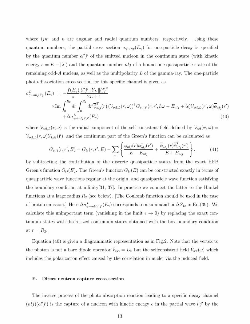
remaining odd-A nucleus, as well as the multipolarity L of the gamma-ray. The one-particle

photo-dissociation cross section for this specific channel is given as

σLγ→nlj,l′j′(Eγ) = −

f(Eγ)

π

〈l′j′‖ YL ‖lj〉2

2L+ 1

×Im

∫ R2

0

dr

∫ R2

0

dr′φT

nlj(r) (Vscf ,L(r, ω))†Gc,l′j′(r, r

′, hω −Enlj + iǫ)Vscf ,L(r′, ω)φnlj(r

′)

+∆σLγ→nlj,l′j′(Eγ) (40)

where Vscf,L(r, ω) is the radial component of the self-consistent field defined by Vscf(r, ω) =

Vscf,L(r, ω)YLM(r), and the continuum part of the Green’s function can be calculated as

Gc,lj(r, r′, E) = Glj(r, r

′, E)−∑

n

{

φnlj(r)φTnlj(r

′)

E − Enlj

+φnlj(r)φ

T

nlj(r′)

E + Enlj

}

. (41)

by subtracting the contribution of the discrete quasiparticle states from the exact HFB

Green’s function Glj(E). The Green’s function Glj(E) can be constructed exactly in terms of

quasiparticle wave functions regular at the origin, and quasiparticle wave function satisfying

the boundary condition at infinity[31, 37]. In practice we connect the latter to the Hankel

functions at a large radius R2 (see below). [The Coulomb function should be used in the case

of proton emission.] Here ∆σLγ→nlj,l′j′(Eγ) corresponds to a summand in ∆S1c in Eq.(39). We

calculate this unimportant term (vanishing in the limit ǫ → 0) by replacing the exact con-

tinuum states with discretized continuum states obtained with the box boundary condition

at r = R2.

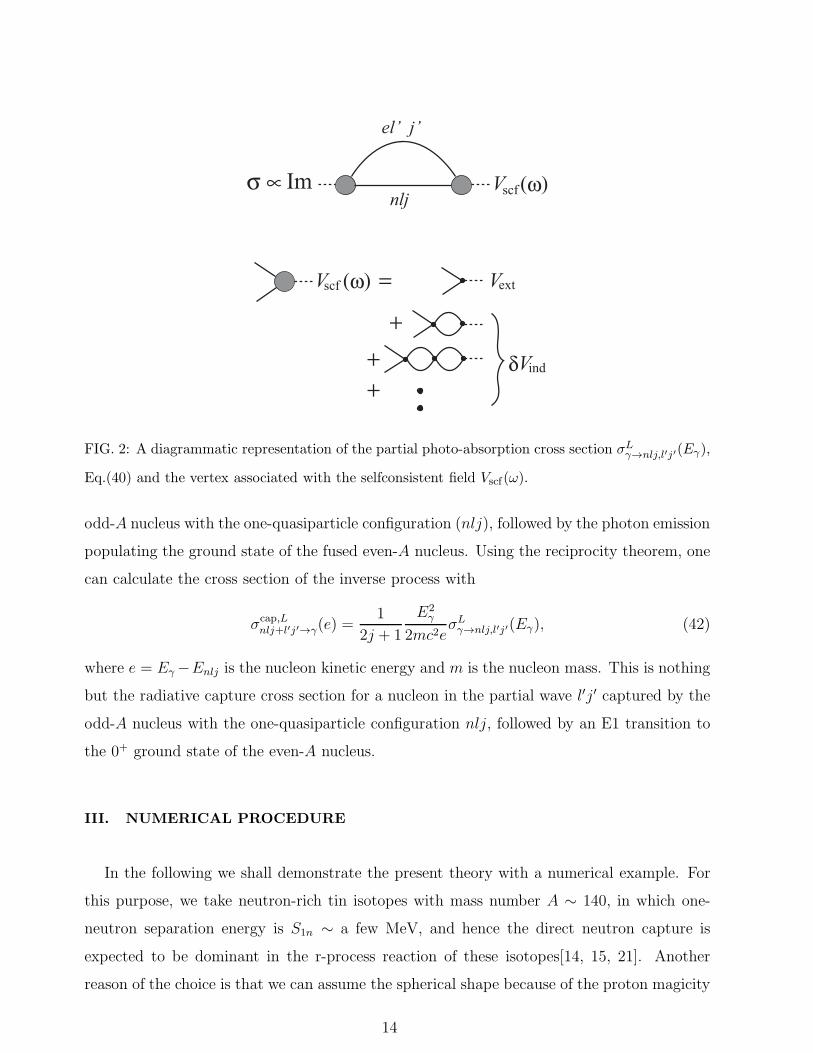
Equation (40) is given a diagrammatic representation as in Fig.2. Note that the vertex to

the photon is not a bare dipole operator Vext = D0 but the selfconsistent field Vscf(ω) which

includes the polarization effect caused by the correlation in nuclei via the induced field.

E. Direct neutron capture cross section

The inverse process of the photo-absorption reaction leading to a specific decay channel

(nlj)(el′j′) is the capture of a nucleon with kinetic energy e in the partial wave l′j′ by the

13

el’ j’

nljV (ω)scf

V (ω)scf =

++

+

V ext

δV ind

Imσ ∝

FIG. 2: A diagrammatic representation of the partial photo-absorption cross section σLγ→nlj,l′j′(Eγ),

Eq.(40) and the vertex associated with the selfconsistent field Vscf(ω).

odd-A nucleus with the one-quasiparticle configuration (nlj), followed by the photon emission

populating the ground state of the fused even-A nucleus. Using the reciprocity theorem, one

can calculate the cross section of the inverse process with

σcap,Lnlj+l′j′→γ(e) =

1

2j + 1

E2γ

2mc2eσLγ→nlj,l′j′(Eγ), (42)

where e = Eγ−Enlj is the nucleon kinetic energy and m is the nucleon mass. This is nothing

but the radiative capture cross section for a nucleon in the partial wave l′j′ captured by the

odd-A nucleus with the one-quasiparticle configuration nlj, followed by an E1 transition to

the 0+ ground state of the even-A nucleus.

III. NUMERICAL PROCEDURE

In the following we shall demonstrate the present theory with a numerical example. For

this purpose, we take neutron-rich tin isotopes with mass number A ∼ 140, in which one-

neutron separation energy is S1n ∼ a few MeV, and hence the direct neutron capture is

expected to be dominant in the r-process reaction of these isotopes[14, 15, 21]. Another

reason of the choice is that we can assume the spherical shape because of the proton magicity

14

S2n

S1n

SLy4Sn even-N

(MeV

)

A

333

333333

110 120 130 140 150 0

5

10

15

333

33

1111111

11

FIG. 3: Calculated one- and two-neutron separation energies S1n and S2n for even-even Sn isotopes,

plotted with solid and dotted lines, respectively. The experimental values[45] are shown with squares

and crosses for S1n and S2n, respectively.

Z = 50 as many Hartree-Fock-Bogoliubov calculations predict[38–40].

We employ the Skyrme energy density functional model and the effective pairing interac-

tion of the contact type to construct the HFB ground state and the associated selfconsistent

mean-field. The adopted Skyrme parameter set is SLy4[41], and the density-dependent delta

interaction of the mixed type[42–44]

v(1, 2) = V0

(

1−ρ(r)

2ρ0

)

δ(r1 − r2) (43)

(ρ0 = 0.16 fm−3) is adopted with the quasiparticle energy cut-off Ecut = 60 MeV and the

orbital angular momentum cut-off lcut = 12. The adopted force strength V0 = 292 MeV fm−3

gives average neutron pairing gap ∆n = 1.25 MeV for stable isotope 120Sn and ∆n = 0.97 MeV

for 142Sn. The proton pairing gap is zero. The radial HFB equation is solved in a spherical

box r < R1 with mesh interval ∆r = 0.2 fm under the box boundary condition φi|r=R1= 0

with the box radius R1 = 20 fm, which is sufficiently large for bulk quantities such as the

total binding energy to converge. The calculation reproduces rather well the experimental

one- and two-neutron separation energies, S1n and S2n, of the even-N tin isotopes, as shown

in Fig.3, and it predicts S1n ≈ 2MeV for A > 140.

15

The continuum QRPA calculation is performed as follows. We adopt the Landau-Migdal

approximation in evaluating the linear response: we consider only the fluctuations in the

local density and local pair density, and we employ the Landau-Migdal parameters F0(r) and

G0(r) in the local density approximation for the particle-hole residual interaction. We solve

the linear response equation

δραL(r, ω) =

∫ R2

0

dr′∑

β

Rαβ0,L(r, r

′, ω)

(

∑

γ

κβγ(r′)1

r2δργL(r

′, ω) + vextβL (r′)

)

(44)

in the radial coordinate space. For the unperturbed response function, we use the

representation[31] using the quasiparticle Green’s function:

Rαβ0,L(r, r

′, ω) =1

4πi

∫

C

dE∑

lj,l′j′

〈l′j′‖ YL ‖lj〉2

2L+ 1{TrAαGl′j′(r, r

′, E + hω + iǫ)AβGlj(r′, r, E)

+ TrAαGlj(r, r′, E)AβGl′j′(r

′, r, E − hω − iǫ)} (45)

in order to treat the continuum quasiparticle states with the proper boundary condition. The

contour C is the one shown in Fig.1(b).

In finding a numerical solution of the linear response equation (44) (using a matrix form

with radial mesh points), and also performing numerical integration in Eq.(40), we need a

large radial space so that we can evaluate the matrix element 〈np(Ep)| Vscf(ω) |0〉 accurately

for scattering state p(Ep) and weakly bound quasiparticle state n. We specify This space is

specified with a radius R2. We found that a choice R2 = R1 = 20 fm provides reasonable

results, which however are not sufficiently converged for the photo-absorption cross sections

with low-energy neutron emission. However, we cannot simply enlarge the HFB cut-off radius

R1 since numerical solution for a quasiparticle state with large quasiparticle energy exhibits

an exponential growth of error when the radial HFB equation is integrated toward large r

(>∼ 25 fm in the present case), as discussed by Bennaceur and Dobaczewski[46]. To avoid

this problem, we adopt the following two prescriptions. i) For the cut-off radius R2 used

in Eqs. (44) and (40), we choose a value larger than R1, while keeping R1 for the HFB

calculation. We neglect the HFB mean-fields in calculating wave functions in the interval

R1 < r < R2 since this potential cut-off is known to stabilize significantly the numerical

solution of quasiparticle wave functions[46]. The potential cut-off can be justified except for

nuclei with very small binding energies ≪ 1 MeV and with very long tails of the density and

the pair density extended to far distances. ii) We introduce a smaller cut-off energy Ecut,out

16

for the upper boundary of the Contour integral in Eq.(45) in evaluating the unperturbed

response function Rαβ0,L(r, r

′, ω) at large distances so that the above numerical problem does

not come into play. In practice, we use Ecut,out = 10 MeV for r′ > R1 while the original cut-off

value Ecut = 60 MeV is used for r′ < R1. We found that this choice gives a convergence with

respect to Ecut,out. We also found that the convergence of the cross section with respect to

R2 is obtained with R2 = 30 fm. In evaluating the unperturbed response function, necessary

for the QRPA calculation, we use a small but finite value of the imaginary constant ǫ = 0.05

MeV, corresponding to a smearing width of 100 keV in the strength function.

One needs to evaluate the partial photo-absorption cross sections and the neutron capture

cross sections with very fine energy resolution if one wants to apply to the astrophysical

problems since the relevant energy scale of the neutron kinetic energy is e ∼ 1 × 10−3 − 1

MeV. For this purpose, we use a very small imaginary constant ǫ = 1 × 10−8 MeV for the

Green’s function appearing in Eq.(40), thus allowing description of the neutron scattering

states with energy resolution ∼ ǫ.

IV. NUMERICAL EXAMPLE

Figure 4 shows the calculated E1 strength dB(E1)/dE ≡ 3∑

k | 〈k|D0 |0〉 |2δ(E − hωk) =

3S(E) plotted as a function of the excitation energy E. A large fraction of the strength is

distributed around E ∼ 10 − 17 MeV, corresponding to the giant dipole resonance. The

strength is also seen between E ∼ 10 MeV and the one-neutron separation energy S1n, and

it is of our interest in this study. Significant fluctuation or fine structure in the GDR region

is seen. They reflect bound proton particle-hole configurations and neutron configurations

involving quasiparticle resonances with narrow width. These fine structures might disappear

if we take into account the spreading width arising from coupling to more complex configu-

rations, e.g. four quasiparticle configurations etc. If we simulate the spreading width using

a finite value of the smearing width, the E1 strength strength distribution becomes smooth

as illustrated by the dashed curve, obtained with the smearing width of γ = 1 MeV.

Figures 5 and 6 show calculated total and partial photo-absorption cross sections. The

total photo-absorption cross section σγ(Eγ), the dotted curve in Fig.5, is proportional to

EdB(E1)/dE|E=Eγ and hence it has basically the same structure as the E1 strength function.

17

E (MeV)

dB(E

1)/d

E(f

m2 M

eV-1

)

142Sn× 2

5 10 15 20 0

5

10

15

20

25

FIG. 4: Calculated E1 strength function dB(E1)/dE in 142Sn. The solid curve is the strength

obtained with a smearing width γ = 2ǫ = 100 keV, while the dashed curve is for a smearing width

of 1 MeV. The long and short arrows indicate the one- and two-neutron separation energies S1n and

S2n, respectively.

Open decay modes of the excited 1− states are one- and two-neutron emissions. The one- two-

neutron separation energies are low: S1n = E3p3/2+|λn| = 2.246 MeV and S2n = 2|λn| = 2.796

MeV, respectively (E3p3/2 is the quasiparticle energy of the neutron 3p3/2 state). The one-

proton separation energy S1p = |e1g9/2 | = 18.191 MeV is located at much higher energy. The

partial photo-absorption cross section for one-neutron emission decay is shown with the solid

curve in Fig.5. It is seen that the partial cross section for two-neutron decay becomes a sizable

fraction for Eγ >∼ 3.5 MeV. The fraction of one-neutron cross section becomes significantly

small as the energy increases although the one-neutron decay survives at energies where the

two-neutron decay channels are open. We remark also that the one-neutron partial cross

section exhibits non-trivial energy dependence which arises from the configuration mixing

in the dipole states. For instance, the fine structures seen around Eγ ∼ 9 − 17 MeV can

be explained only with mixing among proton particle-hole and neutron two-quasiparticle

configurations.

The one-neutron decay is further decomposed into individual decay channels specified with

different neutron configurations. In the present case bound neutron quasiparticle states are

18

Eγ (MeV)

σ γ(Eγ)

(fm

2 )

142Sn

5 10 15 200

2

4

6

8

FIG. 5: Total photo-absorption cross section and partial cross section for one-neutron emission

decay, plotted with dotted and solid curves, respectively, calculated for 142Sn.

3p3/2 and 3p1/2 states with quasiparticle energies E3p3/2 = 0.848 MeV and E3p1/2 = 1.257

MeV while all the other quasiparticle states are in the continuum E > |λn|. Therefore

configurations corresponding to the final states of one-neutron decay are the 3p3/2 state

coupled with continuum s1/2, d5/2 and d3/2 states, combined in total spin and parity 1−

(abbreviated as 3p3/2⊗ cs1/2, 3p3/2⊗ cd3/2 and 3p3/2⊗ cd5/2, hereafter), and similarly, 3p1/2⊗

cs1/2 and 3p1/2 ⊗ cd3/2, involving the 3p1/2 state. The first three are decay channels in which

the one-quasiparticle state 3p3/2, the calculated ground state of 141Sn, is populated while

the last two are those populating the one-quasiparticle state 3p1/2, the only bound excited

state in 141Sn obtained in the present HFB calculation. The partial photo-absorption cross

sections for these decay channels are plotted in Fig.6. The decay channels with population

of the ground 3p3/2 state open at Eγ = E3p3/2 + |λn| = S1n while the channels populating

the 3p1/2 state open at Eγ = E3p1/2 + |λn| = 2.655 MeV, higher than S1n by 409 keV. It

is seen that the probability of populating the excited 3p1/2 state is finite but much smaller

than that populating the ground state 3p3/2. We show in Fig.7 the decay branching ratio. It

is seen that the branching ratio varies with excitation energy, displaying monotonic increase

(decrease) of the two-neutron (one-neutron) decay branches.

Focusing on the ground state decays (the solid curves in Fig.6), we find an apparent

19

Eγ (MeV)

σ γ→m

p(Eγ)

(fm

2 )

142Sn

3p3/2

3p1/2

→ 3p3/2+ cs1/2

→ 3p3/2+ cd5/2

→ 3p1/2+cd3/2

0 2 4 6 80.0

0.1

0.2

0.3

0.4

FIG. 6: Partial photo-absorption cross sections for specific channels of one-neutron emission decay,

calculated for 142Sn. The three solid curves are for channels 3p3/2 ⊗ cs1/2, 3p3/2 ⊗ cd3/2 and 3p3/2 ⊗

cd5/2 while the two dashed curves are for 3p1/2 ⊗ cs1/2 and 3p1/2 ⊗ cd3/2 (see text for details). The

arrows indicate the threshold energies of these decay channels.

feature that the channel with the escaping neutron in the s1/2 wave dominates over those in

the d waves at the lowest energies close to the threshold. At higher energies Eγ >∼ 3 MeV, the

channel with the d-wave neutron dominates.

It is interesting to compare this result with a simple model corresponding to single-particle

transitions in the Hartree-Fock approximation. For the latter, we perform a calculation

neglecting the pairing correlation and the RPA correlation caused by the residual interactions.

In practice we perform the HFB calculation using a reduced paring interaction strength

V0 = 120 MeV fm−3, which leads to a very small average neutron pairing gap ∆n = 0.048

MeV, and calculate the partial photo-absorption cross sections using Eq.(40) in which the

selfconsistent field Vscf(ω) is replaced with the bare dipole operator. The result is shown in

Fig.8 for the decay channels populating the 3p3/2 and 3p1/2 state of the daughter141Sn. (The

cross section for the 3p1/2 state is calculated to be practically zero.)

Several clear differences are seen between Figs.6 and 8. First, the one-neutron separation

energy is higher in the full calculation by about 1.5 MeV than that in the Hartree-Fock

single-particle model. This due to the pair correlation which has an effect to give the even-N

20

Eγ (MeV)

bran

chin

g ra

tio

3p3/2 + 1n

3p1/2 + 1n

2n

3 4 5 6 7 80.0

0.2

0.4

0.6

0.8

1.02

2

2

2

2

23 3

33

3 39

9

9

9

9

9

FIG. 7: Calculated branching ratios for one-neutron decays from photo-excited 1− states of 142Sn

populating the 3p3/2 state of the daughter141Sn (plotted with diamonds), the same but for the 3p3/2

state (squares), and that for two-neutron decays (circles), evaluated for various photon energies Eγ .

nucleus 142Sn more binding energy. The separation energy in the Hartree-Fock approximation

is essentially the single-particle energy -0.883 MeV of the 3p3/2 orbit while the pair correlation

increases the separation energy via the quasiparticle energy E3p3/2 and the Fermi energy

λn. Second, the probability to populate the 3p1/2 state is finite in the full HFB + QRPA

calculation while it is zero in the Hartree-Fock approximation. This is because the single-

particle 3p1/2 orbit is partially occupied in the HFB description of the pair correlated ground

state of 142Sn while the occupation is zero in the unpaired Hartree-Fock approximation.

Third, the cross sections have non-trivial energy dependence in the full calculation while

the energy-dependence in the Hartree-Fock single-particle transitions are quite simple. The

non-trivial energy dependence is due to the RPA correlation and the configuration mixing as

we already mentioned above. The simple structure in the single-particle transitions, on the

other hand, can be understood even in an analytical way[47, 48].

Finally we show in Fig.9 direct neutron capture cross section for 141Sn in the ground state

having the one-quasiparticle configuration 3p3/2 and with the E1 decay populating the 0+

ground state of 142Sn. It is calculated for neutron kinetic energies from e = 1 keV to 8 MeV

using Eq.(42) and the partial photo-absorption cross sections shown in Fig.6. We see that

21

Eγ (MeV)

σ γ→m

p(Eγ)

(fm

2 ) single-particle (HF)

3p3/2 3p1/2

→ 3p3/2+ cs1/2

→ 3p3/2+ cd5/2

0 2 4 6 80.0

0.2

0.4

0.6

0.8

FIG. 8: Partial photo-absorption cross sections for specific channels of one-neutron emission decay,

obtained by neglecting the pairing and RPA correlations. Decays populating the 3p3/2 and 3p1/2

states of the daughter 141Sn are evaluated, but the cross sections for the 3p1/2 state is calculated to

be zero in this null pairing case.

the s-wave capture is dominant at low energies e<∼ 1 MeV as expected. It is also seen that the

energy dependence at very low energies e<∼ 100 keV obeys the power-low scaling σ ∝ el−1/2

(with l being the orbital angular momentum of the partial wave). This threshold behavior

arises from the low-energy asymptotics of the neutron continuum quasiparticle states in the

s1/2, d3/2 and s3/2 waves. Note, however, that their absolute magnitudes as well as behaviors

at higher energies differ from the simple single-particle model, as we discussed above. The

threshold scaling behavior would have been affected if the s- and d-wave neutron had low-

energy resonance or virtual state in e<∼ 100 keV, or if the QRPA correlation would have

exhibited narrow resonances in this energy region. Such situation is not seen in the present

example.

V. CONCLUSIONS

The quasiparticle random phase approximation (QRPA) combined with the Hartree-Fock-

Bogoliubov mean-field model or the nuclear density functional theory is one of the most

powerful frameworks to describe the electro-magnetic responses and the photo-absorption

reaction of neutron-rich nuclei. In this paper, we have extended this framework to describe

the direct radiative neutron-capture reaction of neuron-rich nuclei, one of key reactions in the

22

e (keV)

σ cap(e

)(f

m2 )

s1/2

d5/2

d3/2

10-8

10-7

10-6

10-5

10-4

10-3

100 101 102 10310-8

10-7

10-6

10-5

10-4

10-3

FIG. 9: Neutron capture cross sections for three different entrance channels, consisting of the ground

state with the 3p3/2 configuration of 141Sn and an incident neutron in the partial waves s1/2, d3/2

and d5/2, populating 1− states decaying to the ground state of 142Sn. The horizontal axis is the

neutron kinetic energy e.

astrophysical rapid neutron-capture process. This approach enables one, for the first time, to

take into account the pairing correlation and the RPA correlations in calculating the direct

neutron capture cross section.

We have formulated a method to calculate partial photo-absorption cross sections corre-

sponding to individual channels of one- and two-nucleon emission decays. It is a generaliza-

tion of the method of Zangwill and Soven, originally formulated in the continuum RPA for

unpaired systems, to the case of the continuum QRPA suitable for pair correlated nuclei. We

select one-neutron emission channels in which the decay populates the daughter nucleus in its

ground state. We then use the reciprocity theorem to transform the partial photo-absorption

cross section to the radiative neutron capture cross section. With improved numerical proce-

dure, we made it possible to evaluate the neutron capture cross section at very low neutron

kinetic energies of O(1 keV) and for nuclei with small neutron separation energies. The

theory also enables us to evaluate the branching ratio of the one- and two-neutron emission

decays of the photo-excited states.

Performing numerical calculations for the photo-absorption of 142Sn and the neutron-

23

capture of 141Sn, we have shown that the pairing and the RPA correlations influence the

results significantly. It is shown also that the threshold behavior of the cross sections, gov-

erned by the partial waves of the emitted/incoming neutron, emerges in the present theory.

We remark that in the present work we have neglected the gamma decays from excited

to excited states. For example, we find a low-lying collective 2+1 state below the neutron

separation energy in the present QRPA calculation, but possible E1 transition from the 1−

state populated by the neutron capture to the collective 2+1 state is not described in the

present formalism. It is a future problem to extend the formalism to include this kind of

transitions. We also note that neutron capture of even-N isotopes needs to be described in

a separate way.

Acknowledgment

The author thanks T. Nakatsukasa, K. Ogata and K. Yabana for useful discussion. This

work is supported by Grant-in-Aid for Scientific Research from Japan Society for Promotion

of Science No. 23540294 and No. 26400268.

Appendix A

We shall show a derivation of Eq.(16).

We note first

S(hω) = −1

πIm

∫

dr∑

α

vextα (r, ω)δρα(r, ω)

= −1

πIm

∫

dr∑

α

(

vscfα (r, ω)−∑

γ

καγ(r) (δργ(r, ω))∗

)

δρα(r, ω)

= −1

πIm

∫

dr∑

α

vscfα (r, ω)δρα(r, ω)

+1

π

1

2i

[

∫

dr∑

α,γ

καγ(r) (δργ(r, ω))∗ δρα(r, ω)

−

∫

dr∑

α,γ

κ∗αγ(r)δργ(r, ω) (δρα(r, ω))∗

]

, (46)

24

where

καγ(r) ≡ (καγ(r))∗ sα =

∂2E

∂ρ∗α(r)∂ρ∗β(r)

sα =∂2E

∂ρα(r)∂ρ∗β(r)

. (47)

Using the symmetry

καβ(r)∗ = κβα(r), (48)

we find that the term in the parenthesis in the last expression in Eq.(46) vanishes. We note

also that the linear response equation (13) is written as

δρα(r, ω) =

∫

dr′∑

β

Rαβ0 (r, r′, ω)vscfβ (r, ω). (49)

Inserting this into Eq.(46), we obtain Eq.(16).

Appendix B

In this appendix, we discuss spectral property of Sd(hω) in Eq.(21):

Sd(hω) = −1

πIm∑∑

n>m

{

| 〈nm| Vscf(ω) |0〉 |2

hω − En − Em + iǫ−

| 〈0|Vscf(ω) |nm〉 |2

hω + En + Em + iǫ

}

. (50)

It is tempting to expect delta function peaks at hω = ±(En + Em), the energies of the

two-quasiparticle states consisting of bound quasiparticle states m and n, but this is not the

case.

To show this, we return to the linear fluctuation in the state vector |δΦ(t)〉 =

e−iωt |δΦ(ω)〉+ eiωt |δΦ(−ω)〉 obeying Eq.(8), which reads in the frequency domain

(

hω − h0 + iǫ)

|δΦ(ω + iǫ′)〉 = Vscf(ω + iǫ′) |Φ0〉 . (51)

The strength function Sd(hω) is then written as

Sd(hω) =∑∑

n>m

ǫ

π| 〈nm|δΦ(ω + iǫ′)〉 |2 −

ǫ

π| 〈δΦ(−ω − iǫ′)|nm〉 |2. (52)

We remark here that all the quantities related to the linear response, e.g., |δΦ(ω)〉 and

δρα(ω) inherit the spectral property of the linear response equation (13), which exhibits the

QRPA eigen modes. Therefore, in the discrete energy region hω < S1, the matrix elements

25

〈nm|δΦ(ω)〉 and 〈δΦ(−ω)|nm〉 have poles ∝ 1/(hω ∓ hωk + iǫ), and hence Sd(hω) displays

delta function peaks at the discrete QRPA eigen energies ±hωk in the limit ǫ→ 0:

Sd(hω) =∑

k,hωk<S1

sdkδ(hω − hωk)− sdkδ(hω + hωk). (53)

On the other hand, in the continuum energy region hω > S1, the matrix elements

〈nm|δΦ(ω + iǫ′)〉 and 〈δΦ(−ω − iǫ)|nm〉 are continuous functions of real ω. Therefore Sd(hω)

is proportional to ǫ for sufficiently small ǫ, and it vanishes in the limit ǫ→ 0 and for hω > S1.

[1] T. Sasaqui, T. Kajino, G. J. Mathews, K. Otsuki, and T. Nakamura, Astrophys. J., 634, 1173

(2005).

[2] T. Nakamura et al., Phys. Rev. Lett. 83, 1112 (1999).

[3] M. Arnould, S. Goriely, and K. Takahashi, Phys. Rep. 450, 97 (2007).

[4] P. G. Hansen and B. Jonson, Europhys. Lett. 4, 409 (1987).

[5] Y. Suzuki, K. Ikeda, and H. Sato, Prog. Theor. Phys. 83, 180 (1990).

[6] G. F. Bertsch and H. Esbensen, Ann. Phys. 209, 327 (1991); H. Esbensen and G. F. Bertsch,

Nucl. Phys. A542, 310 (1992).

[7] N. Paar, D. Vretenar, E. Khan, and G. Colo, Rep. Prog. Phys. 70, 691 (2007).

[8] S. Goriely, Phys. Lett. B 436, 10 (1998)

[9] S. Goriely and E. Khan, Nucl. Phys. A706, 217(2002).

[10] S. Goriely, E. Khan, and M. Shamyn, Nucl. Phys. A739, 331(2004).

[11] E. Litvinova, H. P. Loens, K. Langanke, G. Martınez-Pinedo, T. Rauscher, P. Ring, F.-

K. Thielemann, and V. Tselyaev, Nucl. Phys. A823, 26 (2009).

[12] A. Avdeenkov, S. Goriely, S. Kamerdzhiev, and S. Krewald, Phys. Rev. C 83, 064316 (2011).

[13] I. Daoutidis and S. Goriely, Phys. Rev. C 86, 034328 (2012).

[14] Y. Xu, S. Goriely, A. J. Koning, and S. Hilare, Phys. Rev. C 90, 024604 (2014).

[15] G. J. Mathews, A. Mengoni, F.-K. Thielemann, and W. A. Fowler, Astrophys. J. 270, 740

(1983).

[16] S. Goriely, Astron. Astrophys. 325, 414 (1997)

[17] A. M. Lane and J. E. Lynn, Nucl. Phys. 17, 563 (1960).

26

[18] S. Raman, R. F. Carlton, J. C. Wells, E. T. Jurney, and J. E. Lynn, Phys. Rev. C 32, 18

(1985).

[19] A. Mengoni, T. Otsuka, and M. Ishihara, Phys. Rev. C 52, R2334 (1995).

[20] T. Rauscher, R. Bieber, H. Oberhummer, K.-L. Kratz, J. Dobaczewski, P. Moller, and

M. M. Sharma, Phys. Rev. C 57, 2031 (1998).

[21] T. Rauscher, Nucl. Phys. A834, 635c (2010).

[22] S. Chiba, H. Koura, T. Hayakawa, T. Maruyama, T. Kawano, and T. Kajino, Phys. Rev. C

77, 015809 (2008).

[23] Y. Xu and S. Goriely, Phys. Rev. C 86, 045801 (2012).

[24] A. Zangwill and P. Soven, Phys. Rev. A 21, 1561 (1980).

[25] T. Nakatsukasa and K. Yabana, J. Chem. Phys. 114, 2550 (2001).

[26] J. Dobaczewski, H. Flocard, J. Treiner, Nucl. Phys. A422, 103 (1984).

[27] J. Dobaczewski, W. Nazarewicz, T. R. Werner, J. F. Berger, C. R. Chinn, and J. Decharge,

Phys. Rev. C 53, 2809 (1996).

[28] J. Meng and P. Ring, Phys. Rev. Lett. 77, 3963 (1996).

[29] F. Barranco, P. F. Bortignon, R. A. Broglia, G. Colo, and E. Vigezzi, Eur. Phys. J. A11, 385

(2001).

[30] D. M. Brink and R. A. Broglia, Nuclear Superfluidity: Pairing in Finite Systems (Cambridge

University Press, Cambridge, 2005).

[31] M. Matsuo, Nucl. Phys. A696, 371 (2001).

[32] Y. Serizawa and M. Matsuo, Prog. Theor. Phys. 121, 97 (2009).

[33] K. Mizuyama, M. Matsuo, and Y. Serizawa, Phys. Rev. C 79, 024313 (2009).

[34] P. Ring and P. Schuck,The Nuclear Many-Body Problem, (Springer-Verlag, Berlin, 1980).

[35] A. Bohr and B. R. Mottelson, Nuclear Structure vol. II (Benjamin, New York, 1975).

[36] M. Bender, P.-H. Heenen, and P.-G. Reinhard, Rev. Mod. Phys. 75, 121 (2003).

[37] S. T. Belyaev, A. V. Smirnov, S. V. Tolokonnikov, and S. A. Fayans, Sov. J. Nucl. Phys. 45,

783 (1987).

[38] M. V. Stoitsov, J. Dobaczewski, W. Nazarewicz, S. Pittel, and D. J. Dean, Phys. Rev. C 68,

054312 (2003).

[39] J. Dobaczewski, M. V. Stoitsov, and W. Nazarewicz, AIP Conf. Proc. 726, 51 (2004):

27

http://www.fuw.edu.pl/∼dobaczew/thodri/thodri.html

[40] G. A. Lalazissis, A. R. Farhan, and M. M. Sharma, Nucl. Phys. A628, 221 (1998).

[41] E. Chabanat, P. Bonche, P. Haensel, J. Meyer, and R. Schaeffer, Nucl. Phys. A635, 231 (1998);

Nucl. Phys. A643, 441 (1998).

[42] J. Dobaczewski, W. Nazarewicz, and P.-G. Reinhard, Nucl. Phys. A693, 361 (2001).

[43] J. Dobaczewski and W. Nazarewicz, Prog. Theor. Phys. Suppl. 146, 70 (2002).

[44] J. Dobaczewski, W. Nazarewicz, and M. V. Stoitsov, Euro. Phys. J. A15, 21 (2002).

[45] National Nuclear Data Center, http://www.nndc.bnl.gov/

[46] K. Bennaceur and J. Dobaczewski, Comp. Phys. Comm. 168, 96 (2005).

[47] S. Typel and G. Bauer, Nucl. Phys. A759, 247 (2005).

[48] M. A. Nagarajan, S. Lenzi, and A. Vitturi, Euro. Phys. J. A24, 63 (2005).

28