mathematical models of deforestation in the brazilian

Mathematical Models ofDeforestation in the Brazilian

RainforestUCLA Applied Math REU 2019

Bohan Chen, Raymond Chu, Yixuan (Sheryl) He,Joseph McGuire, Kaiyan Peng

Mentor: Christian ParkinsonPI: Andrea Bertozzi, Stanley Osher

University of California, Los AngelesDepartment of Mathematics

Abstract

Identifying two types of deforestation, land clearance for farming and il-legal logging, we develop mathematical models to predict the modes ofdeforestation. Working from first principles, we build individual agentsknown as farmers that then illegally clear forest in the area of concern. Toaccount for illegal logging we develop a continuous model in which loggerstake optimal paths to the location of their crimes, who then must return to"sell" their goods. We discuss some of the optimal control results used inthe illegal logging model, and describe the numerical implementation ofthe illegal logging and farming models. We detail the numerical methodsfor the optimal path and Hamilton-Jacobi equations involved in the model.Finally, we test the effects of different patrol strategies on the occurrencesof illegal logging and measure to what extent they improve the amount ofpristine area.

Contents

1 Introduction 11.1 Previous Work . . . . . . . . . . . . . . . . . . . . . . . . . . . . 1

2 Preparation and Analysis 52.1 Data Analysis . . . . . . . . . . . . . . . . . . . . . . . . . . . . 52.2 Indicator Function of Trees . . . . . . . . . . . . . . . . . . . . 10

3 Farming Model 133.1 Overview of the Farming Model . . . . . . . . . . . . . . . . . 133.2 Fitting Parameters . . . . . . . . . . . . . . . . . . . . . . . . . 163.3 Time Series Model . . . . . . . . . . . . . . . . . . . . . . . . . 18

4 Logging model 224.1 Model Construction . . . . . . . . . . . . . . . . . . . . . . . . . 224.2 Simplification and Approximation . . . . . . . . . . . . . . . . 24

5 Path Planning with Optimal Control Theory 265.1 Static Hamilton-Jacobi-Bellman Equation . . . . . . . . . . . . 265.2 The Eikonal and Hamilton-Jacobi Equations . . . . . . . . . . 275.3 Finding the Optimal Path . . . . . . . . . . . . . . . . . . . . . 285.4 Optimal Control Problem in Our Model . . . . . . . . . . . . . 30

6 Numerical Methods and Implementation 336.1 Numerical Schemes for Hamilton-Jacobi Equations . . . . . . 336.2 The Redistancing Problem for Level Set Equations . . . . . . . 356.3 Implementation Tricks . . . . . . . . . . . . . . . . . . . . . . . 37

7 Logging Experiments 407.1 Experimental Setup . . . . . . . . . . . . . . . . . . . . . . . . . 407.2 Results . . . . . . . . . . . . . . . . . . . . . . . . . . . . . . . . 42

7.2.1 Example 1: No Patrol . . . . . . . . . . . . . . . . . . . 427.2.2 Example 2: Comparison of Different Budget . . . . . . 437.2.3 Example 3: Influence of Patrol on Logging Time . . . . 437.2.4 Example 4: Comparison of Different Patrol Strategies . 447.2.5 Example 5: Optimal Paths . . . . . . . . . . . . . . . . . 48

8 Conclusion 528.1 Farming Model: Main Achievements and Future Work . . . . 528.2 Logging Model: Main Achievements and Future Work . . . . 52

Bibliography 55

1. Introduction 1

1 Introduction

Deforestation, and in particular, illegal logging and land clearance havesome of the most damaging effects on the world’s forest. Modeling andquantifying deforestation has become a recent area of study for ecologists,political scientists, and applied mathematicians. The efficient and effectivedeployment of law enforcement to the threatened area is the best deterrentfor these crimes [1]. Building a model to predict the interactions betweenthe criminals and police is a difficult problem. A crucial first step in thisproblem is identifying significant parameters to consider.

Rigorous studies have validated the correlation between certain param-eters and deforestation in tropical regions such as Brazil [21]. The threedominant categories of parameters are identified by Pfaff and other au-thors, as accessibility, population, climate, and demand [3, 13]. Accessibil-ity accounts for distance to roads, rivers, and major highways, elevation,the presence of trees or foliage, as well as recent deforestation events in thearea. Population density accounts for distance to cities and markets, as wellas the presence of farms and other rural settlements. Climate and demandfactors refer to the seasonal effect, such as precipitation and the global de-mand of soy, beef, lumber and other commodities. With these significantparameters identified, the goal is to inform law enforcement agencies as tothe best strategies for combating deforestation.

Further analysis of enforcement strategies has been carried out in thestate of Roraima, Brazil, using satellite imaging built to detect deforesta-tion events [7, 23]. The strategy on the part of the federal government ofBrazil was to monitor deforestation events in each municipality and dis-patch federal patrols to the municipalities with the most events. The satel-lite data employed (DETER), was updated daily and was effective in detect-ing any deforestation events larger than 25 hectares in size. This particularmacro-strategy proved more effective than typical enforcement strategies,however, the issue remains of how to identify effective microscopic patrolstrategies for law enforcement.

1.1 Previous Work

A similar question was asked and answered with a game-theoretic model,Protection Assistant for Wildlife Security (PAWS), where an iterative Stack-elberg security game was used to describe the interactions between wildlifepoachers and rangers [9]. Previously repeated Stackelberg security games

1. Introduction 2

were utilized to model the protection of vital infrastructure in the case ofattack. PAWS employed a discrete approach to determine effective patrolstrategies in an area of interest. Machine learning techniques were usedto determine animal density for each cell in the grid, as well as assign anaccessibility score to each cell. Cells that were topographically significant,i.e., cells necessary to enter or exit a region, or cells with high accessibil-ity score, were designated key access points. These were then deemed asnodes and edges were drawn to connect the nodes, so that cells with ahigher accessibility score were traversed when possible. Other considera-tions such as time of patrol and the inclusion of base camp from where tostart and end were included for realism, as well as an uncertainty of animaldensity based on the time of last patrol in that cell. Similar algorithms suchas INTERcept and SHARP have been developed and deployed around theworld with varying success [11, 12].

In a paper by Albers [1], the problem of deforestation was modeledin a spatially continuous setting. The author of this paper considered acircular area of interest, and modeling how deforestation and patrollingagainst this, might be described. The patrollers are allocated a budget E,meant to represent the resources available. Budget is used to determinea patrol strategy for the defenders. This is done by giving each radiusr a probability of detection φ(r), then the chance of the attackers gettingcaught as they are moving from distance dc to d is given by:

Φ(d) =∫ d

dc

φ(r)dr

The attackers are assumed to move in radially from their starting radius,dc, and any ground touched by the attackers is now considered unpristine,while the remaining land is termed pristine as seen in figure 1b. Addition-ally, the profit that the attackers received by moving a distance d into theprotected area is given by:

P(d) = (1−Φ(d))B(d)− C(d)

where B is the benefit to the attacker, C is the cost of traveling into depth dand (1−Φ(d)) represents the probability of not being captured.

A rational attacker will find the d that solves the following optimizationproblem:

maxd

(P(d))

The defenders then want to minimize the d that solves this problem.

1. Introduction 3

(a) Level sets evolving to a time t (b) Albers’ radial evolution

Figure 1: Level set method and Albers’ curve evolution

Some issues with this model are the assumption that the area involvedis circular, the lack of terrain information, and the uniform behavior of theattackers and defenders. These problems are addressed in a paper fromArnold et al. [2], where a similar modeling problem is generalized to anyclosed, simple curve in R2. The primary tool employed in this model is thelevel set method [19]. Starting with a closed, simple curve Γ, a Lipschitzcontinuous function is defined, such that φ0 : R2 → R, where φ0(x, y) ispositive inside Γ, negative inside of Γ, and zero at the boundary. Note thatthese requirements on φ0 are satisfied by the signed distance function tothe curve Γ, where distance outside of the curve is negative and positiveoutside. The function φ : R2 × [0, ∞) → R is then defined by the initialvalue problem:

φt + v(x, y)|∇φ| = 0φ(x, y, 0) = φ0(x, y)

where v(x, y) is some non-negative velocity function. Next we define thezero level set Γ(t) = (x, y) | φ(x, y, t) = 0 and this contour represents theset of points that can be reached from the original contour Γ after travelingtime t. In this model cost represents the effort expended by extracting atany point in the protected area, and the velocity is allowed to depend oncapture probability and terrain data. The validity of this model hasn’t beentested against real-world data, but has been modified and improved byCartee and Vladimirsky [5].

The purpose of this project is to use the data gathered and categorizedby Slough et al. [23] to build a predictive continuous model to describe de-forestation events in the state of Roraima. Further, we attempt to determineeffective patrol strategies for law enforcement on microscopic scale, and im-prove upon the model of Arnold et al. [2]. First, we will explain some of

1. Introduction 4

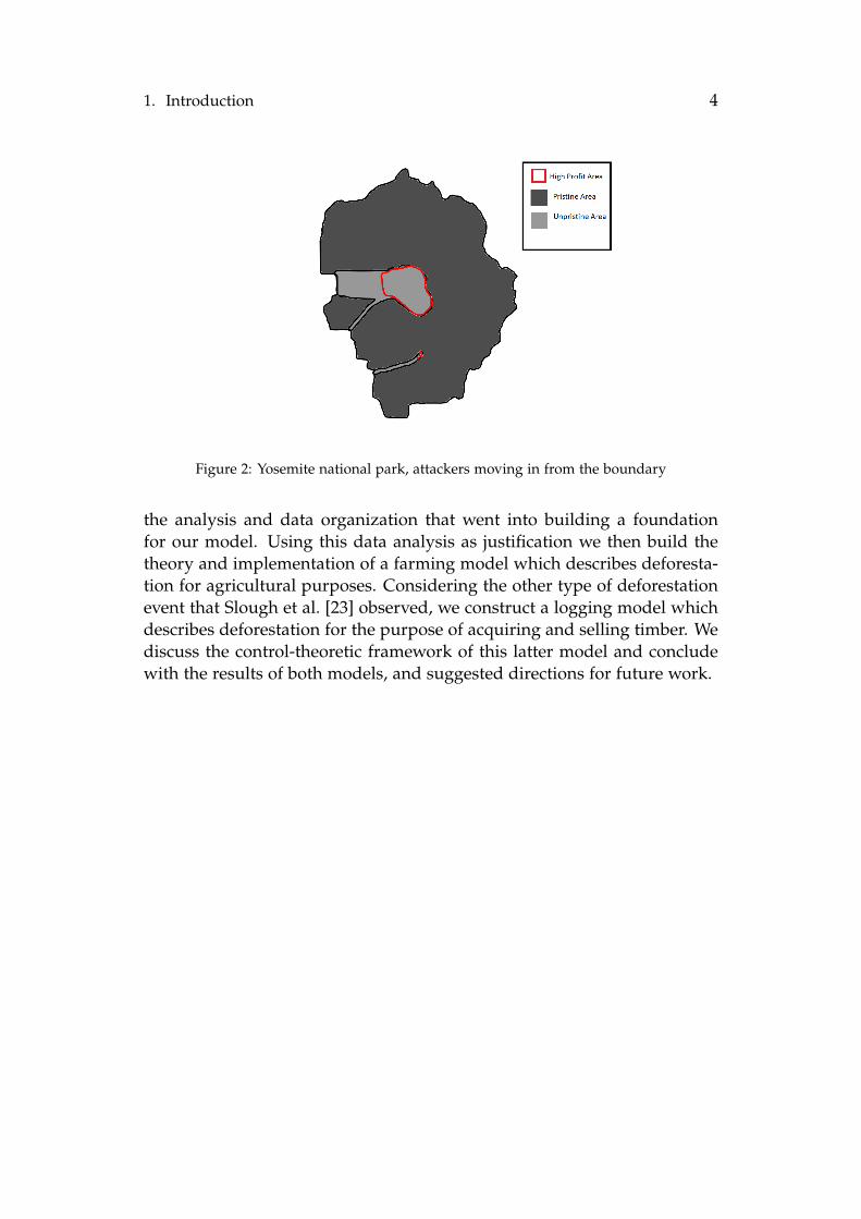
Figure 2: Yosemite national park, attackers moving in from the boundary

the analysis and data organization that went into building a foundationfor our model. Using this data analysis as justification we then build thetheory and implementation of a farming model which describes deforesta-tion for agricultural purposes. Considering the other type of deforestationevent that Slough et al. [23] observed, we construct a logging model whichdescribes deforestation for the purpose of acquiring and selling timber. Wediscuss the control-theoretic framework of this latter model and concludewith the results of both models, and suggested directions for future work.

2. Preparation and Analysis 5

2 Preparation and Analysis

In the beginning of the project, we were given a data set named DETER.The purpose of DETER is to monitor and prevent deforestation in Brazil,specifically Mucajaí, a municipality within the state of Roraima, Brazil [23].In the DETER data set, the space is discretized with polygons and eachpolygon is assigned a Boolean value to determine whether or not a defor-estation event occurred in that polygon in each year and month. Informa-tion such as distance to roads and distance to river for each polygon is alsoincluded. This set contained data from 2006 to 2015.

We then found another data set, PRODES [15]. This data set is theofficial data set the Brazilian Government uses to make annual statistics re-lating to deforestation. The major difference between DETER and PRODESis that the purpose of PRODES is to observe deforestation to make annualstatistics. PRODES only includes yearly data from 2001 to 2015.

2.1 Data Analysis

Our goal was to use both of these data sets to generate an accurate modelof deforestation in Brazil. Our first step was visualizing the data set tohave a better intuition for deforestation in Brazil. In figure 3 we plot thelocation of deforestation events, a portion of the roads and all the riversnear Mucajaí. One of the first observations we made about the data set isthat most deforestation events happen near the roads and the events thatare farther away tend to be very close to the rivers. In fact, 90 percent ofthe deforestation events from the PRODES data set lie within 5 km of theroads. This observation makes sense as proximity to the roads or riversreduces the time it takes to travel to the extraction site and the city, whichreduces the cost an extractor associates with going to the extraction site.

After this observation, we wanted to generate a probability densityfunction (PDF) from the data set. Suppose we are given a set of pointsxiN

i=1 where N is very large (for the PRODES data set N ≈ 36, 000) sam-pled from a PDF φ. Then we would like to reconstruct φ from these sam-ples. This is an ill-posed problem since there are infinitely many PDFs thatcould give rise to the data. For instance one popular method known askernal density estimates (KDE) fixes a PDF f with its mass centered at 0,then fixes a parameter h > 0 called the bandwidth. The predicted PDF is


Figure 3: Dark blue is rivers, black is a subset of roads, light blue is area close to Mucajaí,and red dots correspond to deforestation events

defined by

Φ(x) :=1

Nh2

N

∑i=1

f(

x− xi

h

)Thus Φ is a PDF where the points xiN

i=1 were very likely to be chosensince f mass is centered at the origin. A popular choice of f is the standardGaussian. We implemented this method with f as the standard Gaussianand h = 3 km. In figure 4 we plot a heat map of the PRODES data setwith the color being dependent on Φ. The more yellow spots correspondto larger Φ.

Another popular method is maximizing a regularized logarithmic like-lihood. We first motivate the maximization of log likelihood. AssumexiN

i=1 was drawn independently and identically distributed with densityφ. Then our goal is to find a PDF Φ such that it maximizes the chances ofxiN

i=1 being chosen and use Φ as an approximation for φ. Observe thatas xi are assumed to be independent

P(xiNi=1) = ΠN

i=1P(xi)


Figure 4: KDE with standard Gaussian and h = 3 km on PRODES data set

i.e., the probability of choosing the set xiNi=1 is equal to the product of

choosing each event. We now take logarithms on both sides to convert theproduct into a sum:

log(P(xiNi=1)) =

N

∑i=1

log(P(xi))

Since log(x) is an increasing function, maximizing the probability of the setbeing chosen is equivalent to maximizing the log likelihood ∑N

i=1 log(P(xi)).The maximum log likelihood method approximates φ by

φ ≈ arg maxv,v≥0,

∫v=1

N

∑i=1

log(v(xi))

However, this maximization problem tends to be lead to non-smooth PDFs.Accordingly, the method of maximized penalty likelihood estimate (MPLE)actually defines

φ ≈ arg maxv,v≥0,

∫v=1

N

∑i=1

log(v(xi))− f (v, x) (1)


where f is a regularization term added to increase smoothness of the ap-proximation PDF. It has been observed that the PDFs generated by MPLEwith sharp gradient changes lead to the PDF being not smooth, so a popu-lar f is

f := −α∫

Ω|∇v|

where α > 0 and Ω is the spatial domain we are interested in. This reg-ularization term helps reduce sharp gradient changes, which leads to asmoother PDF.

To approximate a solution to (1), we followed [14] and considered thefollowing discrete version of (1)

arg minv≥0

∑i,j|∇vi,j| − µ ∑

i,jwi,j log(vi,j)

subject to ∑

i,jv = 1 (2)

where w is a weight matrix and ∇v :=(

vi+1,j−vi,j∆x ,

vi,j+1−vi,j∆y

)and µ > 0.

We solve this constrained optimization problem by adding two penaltyfunctions for each constraint

arg minv≥0

∑i,j|di,j| − µ ∑

i,jwi,j +

λ

2 ∑i,j|di,j −∇vi,j|+ γ(1−∑

i,jvi,j)

2

where λ, γ > 0 are fixed. These are punishment terms for not satisfyingthe constraints. To more strongly enforce this constraint, the authors of [14]solved

(uk, dk) = arg minv≥0,d

∑i,j|di,j|−µ ∑

i,jwi,j +

λ

2 ∑i,j|di,j −∇vi,j − bk−1|

+ γ(1−∑i,j

vi,j − bk−11 )2

where

bk = bk−1 +∇uk − dk

bk1 = bk−1

1 + ∑i,j

uki,j − 1


These vectors bk and bk1—the so-called ’Bregman’ vectors—are initialized

so b1 = b11 = 0. These vectors introduce a harsher penalty to the min-

imization problem for straying away from the constraints. Then we usedthe authors’ code to solve this minimization problem which converges withspeed O(n2). The authors recommended the usage of µ = 10−4, λ = 2µn4,and γ = 2µn2. We tested this choice of µ with a 10-fold cross validation forµ = 10−i for i = 0,. . . , 10 and found that µ = 10−4 was optimal.

Figure 5: MPLE with µ = 10−4 on PRODES Data Set

In figure 5 we plot a heat map of MPLE. The red locations correspondto larger values of the density function. To check the accuracy of MPLE, wegenerated random events with the MPLE PDF and compared it to real data.We plot the results of this random sampling in figure 6. This figure showsthat the predicted event locations from MPLE are almost identical to theactual data, which leads us to believe MPLE is a good PDF approximationfor our purposes.

We also used the DETER data set to see if there is a seasonal componentto deforestation. In figure 7, we plot the average percentage of deforestationthat occurs in each month. This bar graph shows that in May to July thereis a strong drop in deforestation compared to other months. Those monthscorrespond to the rainy season in Mucajaí, confirming our suspicions thatthe data expresses seasonality.


(a) Deforestation location predictedby MPLE

(b) Deforestation location fromPRODES

Figure 6: A comparison of PRODES deforestation data and synthetic data generated fromthe MPLE density function

1 2 3 4 5 6 7 8 9 10 11 12

Months

0

0.02

0.04

0.06

0.08

0.1

0.12

0.14

0.16

0.18

Avera

ge P

erc

enta

ge o

f D

efo

resta

tion

Figure 7: Seasonality of Deforestation in Mucajaí

2.2 Indicator Function of Trees

Since we are trying to model deforestation events, we need to know exactlywhere the trees are. Therefore, we need to define the indicator function oftrees for all grid points in our region of interest. The PRODES data setprovides some information about tree coverage locations, so we use the


PRODES data with some modifications to obtain our indicator function oftrees over the years from 2001 to 2015. The specific algorithm we use toconstruct the indicator function of trees for each year is as follows:

1. Use the previous year’s forest coverage location data for the nextyear’s initial indicator function of trees. For example, we use year2004’s forest coverage location data for the year 2005’s initial indica-tor function of trees. For n = 2009, . . . , 2015, we denote the initialindicator function of trees in year n to be χ0

trees,n. We only use such nbecause PRODES data set only provides forest coverage location datafor the years 2008 to 2014 in our region of interest.

2. Get the modified indicator function of trees for the year 2009 by set-ting the locations where deforestation happened in year 2009 to be 1.That is, the modified indicator function of trees for the year 2009 is

χ1trees,2009 = min(1, χ0

trees,2009 + χevents,2009),

where χevents,2009 is the indicator matrix of events in the year 2009.

3. For years from 2008 to 2001, we trace backwards. That is, for n =2008, 2007, . . . , 2001, we first let χ0

trees,n = χ1trees,n+1. Then we get the

modified indicator function of trees for the year n by setting the loca-tions where deforestation happened this year to be 1:

χ1trees,n = min(1, χ0

trees,n + χevents,n).

4. For years from 2010 to 2015, we get the modified indicator functionof trees for the year n by setting the locations where deforestationhappened this year to be 1:

χ1trees,n = min(1, χ0

trees,n + χevents,n).

5. Obtain the final indicator function for trees in the year 2015 as χtrees,2015 =χ1

trees,2015.

6. Make sure that the indicator function will not increase over the years,by taking the maximum of two consecutive years to modify indicatorfunctions of trees backwards. That is, for n = 2014, 2013, . . . , 2001, wetrace back to get the final indicator function for trees to be χtrees,n =max(χ1

trees,n, χtrees,n+1).


(a) Indicator function of trees for 2001 (b) Indicator function of trees for 2015

Figure 8: Indicator function at the beginning and end of the time period

Figure 8a and 8b show the indicator function of trees for the year 2001 and2015. The yellow color denotes value 1 and blue denotes value 0 for thefunction. There is significant difference inside the red box as trees havebeen added as we trace back to 2001.

3. Farming Model 13

3 Farming Model

Slough et al. [23] concluded that there are two main types of deforestationthat occur in Roraima. The first type is agricultural deforestation, whereinfarmers illegally expand their farms to increase their crop output. In thissection, we describe how we model this phenomenon. The second type ofdeforestation is illegal acquisition and sale of timber. This is addressed insection 4.1.

As mentioned in the previous section, we observe that most deforesta-tion events occur near the roads or cities. Further, in the southeast portionof Roraima, there is a region with many roads and small cities. We focuson modelling illegal farming in this region, pictured in figure 9.

Figure 9: The southeast region of Roraima where we test our farming model.

3.1 Overview of the Farming Model

We first assume that the farmers have perfect information regarding pa-trol. Also, farmers choose locations for farms probabilistically based onexpected profit. To define the expected profit, we first have to define thecost and expected benefit.

Because most events happen near cities and along the roads the cost hasdependence on the distance to cities and distance to roads. In addition, weobserved that the deforestation events tend to cluster around one another.Therefore, we defined the cost at each point per month in the year n as

3. Farming Model 14

C(x, y) =c1 · dr(x, y) + c2 · dc(x, y) + c4

1 + c3 · An(x, y), (3)

where dr(x, y) denotes the distance to roads at location (x, y), and dc(x, y)denotes the distance to cities at location (x, y). The distances are calculatedfrom the center of a farm to the nearest road or nearest city. The measure-ment of fixed costs associated to running a farm is denoted as c4. Note thatc1, c2, c3, c4 ≥ 0 can be adjusted to fit the deforestation data. The final cal-culation of expected profit should be the sum of all costs in related months.This is because there exist ongoing costs when farmers are travelling backand forth. The accessibility at location (x, y) in the year n is denoted asAn(x, y). For Accessibility, we first define (x(n)i , y(n)i )M(n)

i=1 as the defor-estation events which occurred in the year n. Then we fixed a parameterh > 0 called the bandwidth and define the accessibility contributed by theyear n as

Anh(x, y) :=

M(n)

∑i=1

12πh

exp

− (x− x(n)i )2+ (y− y(n)i )

2

h2

(4)

Finally we obtain the accessibility for location (x, y) in the year n as

An(x, y) :=3

∑k=1

12k An−k

h (x, y) (5)

So accessibility is a weighted sum of Gaussian with expected values atthe deforestation locations and standard deviation h where the influenceof each Gaussian decays over time by a factor of 1

2 for each year that haspassed and we consider only the previous 3 years events. This assumesthat farmers develop infrastructure as they plant farms, reducing costs fornearby farms.

Now we move on to define expected benefit. First we defined the benefitper square meter per month by:

B(x, y) := ξχtrees(x, y)1

1 + ||∇E(x, y)||γ

where χtrees(x, y) is the indicator function for the presence of a tree atlocation (x, y), E(x, y) is the elevation, and ξ represents the conversionof the value of a tree to currency. Typically, we choose ξ = 5000. Wescale this factor by 1

1+||∇E(x,y)||γ because if the area has sharp changes in

3. Farming Model 15

elevation, then it will be harder to farm, while if it is almost flat then||∇E(x, y)|| ≈ 0⇒ B(x, y) ≈ ξχtrees(x, y).

Benefit and cost are not the only factors that farmers consider whenchoosing a farm location. They also account for the probability of gettingcaught illegally making and expanding their farms in their expected benefitcalculation. In any given month, we model the probability of not beingcaptured by

1− ψ(x, y) · Swhere ψ(x, y) is capture probability at location (x, y) (dependent on patrol)and S is the area of the farm.

Assume a farm starts with area S0, and expands for i months at a rateof dS, then the size of the farm at the end of the ith month will be Si =S0 + i · dS. As the minimum area of deforestation in PRODES is about 10square meters and the average is about 105 square meters per year, wechoose S0 = 10, dS = 105

12 . Thus, the probability of not being captured bythe end of the ith month at location (x, y), if we assume that the captureprobability in different months are independent, is

βi(x, y) =i

∏j=1

(1− ψ(x, y) · Sj).

The expected benefit farmer will receive in month i is

E(Benefiti(x, y)) = B(x, y) · Si · βi(x, y)− α · B(x, y) · Si · (1− βi(x, y))

Here α > 0 is a parameter that measures the strength of punishment. Forexample, α = 2.5, means that if a farmer is caught, then he will be finedwith the amount of 2.5 times the benefit he will gain from that farm inmonth i. And the expected benefit which a farmer will receive by the endof month i is

i

∑j=1

E(Benefitj(x, y))

As a farm cannot last forever partly due to lack of nutrition in the land,we assumed that a farm can only operate for at most Kmax months. For ourexperiments, we choose Kmax = 36. Therefore, a farmer will chose a monthbetween 1, .., Kmax such that they maximize their expected profit.

Thus, the expected profit function for a farmer is

E(P(x, y)) :=

(max

i=1,...,Kmax

i

∑j=1

(E(Benefitj(x, y))− C(x, y)

))+

3. Farming Model 16

where ( f )+ := max( f , 0). So if farmers choose a spot (x, y), then they willstay in that spot until they gain the expected highest profit or until getcaught.

Then we normalize E(P(x, y)) to make it into a probability density func-tion. Farmers will choose where to plant their farms randomly with thisdensity.

3.2 Fitting Parameters

To fit the model to our data, we try to optimize our set of parameters bymaximizing the average F1 score, as defined later in this section. Notethat we are fitting the parameters using the predicted model and PRODESdata from 2005 to 2015, on the bottom right part of the region described inPRODES, as in Figure 9. The range of area is [-61.3, -58.8868] in longitudeand [-0.1293, 1.54] in latitude. We fit 500× 500 grid points in this region togenerate our results and fit the parameters.

Due to sparsity of the events, the way we define true positive instancesshould have some tolerance of position offset. Specifically, given a pre-dicted probability density function for illegal farming, the true data pointswhere events happen in the region from 2005 to 2015, and a threshold,we claim that an event is truly predicted if for a square centered at theevent point, there is at least one point within the square with predictedprobability density function value larger than or equal to the threshold.

First we denote the grid points to be (xi, yj), for i, j = 1, . . . , 500. Thenwe define the matrix that counts the number of events in each grid in theyear n by NEn, where NEn(xi, yj) is the number of real events in year nwhose location has (xi, yj) as the nearest grid point. Denote the probabilitydensity function generated by the expected profit for the year n to be f n.Then the event prediction function can be defined as

pn(xi, yj) := χ f n(xi,yj)>ε·NEn(xi,yj)· χNEn(xi,yj)>0,

where ε is the threshold for prediction, and χ is the indicator function.For a grid point to have events, we require NEn(xi, yj) > 0. To account formultiple events, we require f n(xi, yj) > ε · NEn(xi, yj), which means that ifthere are, for example, two events at a grid in the year n, then to claim thata grid point is predicted, we require the probability density function by theexpected profit to be at least twice that of the threshold.

Now we define the notion of true positive and false positive. To dealwith sparsity of the events, we define the true positive function for the year

3. Farming Model 17

n bytpn(xi, yj) := maxpn(x, y) : (x, y) ∈ U(xi, yj),

where U(xi, yj) is a neighborhood of the point (xi, yj). For our experi-ment, we take a square centered at (xi, yj). That is, we define U(xi, yj) :=(xi+di, yj+dj) : di, dj = −4, . . . , 4, i + di, j + dj ∈ [1, 500]

.

To define the false positive function, we omit the tolerance region. Thatis, we define the false positive function for the year n by

f pn(xi, yj) := χ f n(xi,yj)>ε · χNEn(xi,yj)=0.

Therefore, the number of true positive points and false positive pointsin the year n can be calculated as TPn := ∑500

i=1 ∑500j=1 tpn(xi, yj) and FPn :=

∑500i=1 ∑500

j=1 f pn(xi, yj) respectively.The recall (true positive rate) for the year n can then be calculated as

Rn :=TPn

number of events in year n=

TPn

∑500i=1 ∑500

j=1 NEn(xi, yj),

and precision for the year n can then be calculated as

Pn :=TPn

number of ’predicted’ events in year n=

TPn

TPn + FPn .

The ’predicted’ here is not quite well-defined, as we consider a toleranceneighborhood only for true positive events but not for false positive events.However, by summing over the number of true positive events and falsepositive events, we can approximate the notion of the number of ’predicted’events.

Finally, we have the F1 score for each year:

F1n :=2 · (Pn · Rn)

Pn + Rn . (6)

We then average the F1 scores to obtain the average F1 score for the pre-dicted model, and optimize parameters c1, c2, c3, c4, cp, γ, ε and α to achievethe highest average F1 score, where ε is the threshold we use to define thetrue positives. Here, cp is a parameter to fit in our initial model, wherewe use ψn = cp ·m f n−1, and m f n−1 is the probability density function fordeforestation events generated using the MPLE method from PRODES forthe region in the previous year, year n− 1. The optimized set of parameterswe find is c1 = 1

1000 , c2 = 110000 , c3 = 10, c4 = 10, cp = 1, γ = 1, ε = 10−5;

3. Farming Model 18

and α = 2.5. These yield an average F1 score of 0.59. This score is notperfect because of the sparsity of real deforestation events, but the aver-age recall (true positive rate), which measures the ability of our model topredict where events will happen, is 0.72, which is better.

3.3 Time Series Model

In the farmer’s model so far, the Profit density has been static. Now we con-sider a simulation wherein multiple farmers plant their own farms. Thenthe benefit near their selected farm should decrease as the next farmerscannot farm there. Hence, the Profit density should be updated based oneach farmer. Accordingly, we want to design a time series model with thegoal of accurately predicting deforestation events caused by farmers.

We assume that for a fixed year N that we have data about the deforesta-tion events for year N− 1, N− 2 , and N− 3 and a patrol density ψ(x). Wefirst generate an initial Profit PDF by following the procedures in section(3.1). Now we randomly generate a point x1 ∈ Ω according to the profitPDF where Ω is our spatial domain. This node x1 represents the locationof where the first farmer of this year decided to plant a farm. In particular,we assume that the farmer creates a square farm centered at x1 with length√

S0 (and hence area S0). Now we expect the benefit to decrease near thisfarm, so if we fix K ∈ [0, 1), and let S1 denote square farm belonging to thefirst farmer, then we do the following update to benefit:

B(x) = B(x) ·min1, K + dist(x,S1)

This update decreases the benefit linearly based on distance to the farmwith points in the farm benefit being decreased by the factor K. In practice,we chose K = 1

2 and we choose to keep K > 0 because in our data set,multiple events happened on the same node which is due to the coarsenessof our grid. In addition, as the farmer constructs a farm at x1 we expectthis farmer to create infrastructure which makes it more accessible for otherfarmers to get near x1. Therefore, we update accessibility by the followingformula

A(x) = A(x) +1

2πhexp

(−||x1 − x||2

h2

)Then we normalized A so that it retains its initial mass.

Now we also assume that farmer 1 wants to expand his farm’s area bydS by the end of this month, but as this activity is illegal, there is a chance

3. Farming Model 19

he can get caught while expanding their farm. To simulate this we do aBernoulli trial with probability p = ψ(x1) · S0. If the trial is successful,the farmer is caught, so he does not expand his farm and he also receivesa fine of αB(x1)S0. Otherwise, if the trial is a failure, the farmer is notcaught and expands his farm to by a constant factor dS. Now we use theupdated benefit and accessibility score to update the Profit PDF. We repeatthis procedure for all the farmers we want to simulate in the first month.

Generated Data For 2015

(a) Time Series Model for 2015

2015 real data

(b) Data from PRODES data set for 2015

Figure 10: Time Series Generated Data compared to Real Data

Now assume we are in month i where 1 < i ≤ 12. We update ψ to ac-count for changes in patrol strategy. Next we define N(i) to be the numberof farmers released in the simulation from month 1 to the end of month i,Sj denote the farm of the jth farmer, and xj as the center of the square farmof farmer j. Now for 1 ≤ j ≤ N(i − 1) we simulate a Bernoulli trial withp = |Sj|ψ(xj) to determine whether or not they get caught expanding theirfarm this month. Then we update the Benefit generated by each farmer jfor each new node inside Sj and update the Profit. We repeat the initialprocedure with this updated Profit to generate new farmers location andrepeat this process for all desired months. In figure 10 we plot the TimeSeries prediction for centers of the farms created in 2015 compared to thedeforestation events that occurred in 2015 according to PRODES data. Infigure 11 and 12 we plot an exaggerated square farms corresponding tothe farms the farmer chose in the months June and December. The redcross indicates the farmer got caught expanding their farm, and we had 34farmers getting caught in the simulation for 2015 out of 626 extractors.

3. Farming Model 20

Month 6.000000

Figure 11: Result of time series simulation in June of 2015. Black boxes correspond tofarms and red crosses means the farmer was caught. The sizes of the farm has beenexaggerated to make farms more visible.

3. Farming Model 21

Month 12.000000

Figure 12: Result of time series simulation in December of 2015. Black boxes correspondto farms and red crosses means the farmer was caught. The sizes of the farm has beenexaggerated to make farms more visible.

4. Logging model 22

4 Logging model

Illegal logging is another contributing factor to deforestation, which ex-hibits quite different behavior from farming. Loggers obtain profit fromtimber rather than land. They may go deeper into the forest where treesare more valuable. Judicious path planning that balances both travel timeand capture risk then plays a major role in loggers’ decision making. In ourmodel, we assume that deforestation events at least 10 km from the high-ways are logging events. We build up a more realistic model to describeloggers’ decision making process which can be useful to evaluate, compareand design patrol strategies.

Our logging model is based on Albers [1] where loggers want to maxi-mize their expected profit P, defined as

P = ΦB− C.

Here B is the pre-determined initial benefit that depends on the categoryand quality of timber and is assumed to be static. C represents the cost andis measured by the traveling time of both going in and out of the forest.Φ describes the probability of not being captured, which depends on pa-trollers’ detection ability and loggers’ trajectories. We follow the Stakelberggame model and assume loggers have perfect information about patrol.

Diverging from previous models where extracting happens instanta-neously, we introduce the notion of logging time. Actual logging time willinfluence the risk of being detected and the amount of trees loggers canobtain. The latter will further influence the travel velocity when loggersreturn from the forest.

The loggers then need to choose the optimal logging spot, along withlogging time and traveling path. To address the resulting optimizationproblem in random domain geometries, we transform the optimal pathplanning problem into a time-dependent Hamilton Jacobi equation andappeal to the level set method as in Arnold et al. [2]. We then perform aparameter sweep to find the optimal logging location and time.

In section 4.1 we will fully formulate the problem. The resulting opti-mization problem will be further addressed in section 5.

4.1 Model Construction

We assume each location x in the domain Ω ⊂ R2 has a fixed amount oftimber, but with different total value B(x). Different from previous mod-

4. Logging model 23

els where logging happens instantaneously, we use t to denote the actuallogging time. Under the constant production rate assumption, t

T B(x) givesthe actual benefit if there were no patrollers, where T is a global constantrepresenting the time to clear all the trees in one location.

Loggers can be detected when they are logging or on their path backwhile returning with their illegal goods. We assume that the capturingevent is a Poisson process, with (capture) intensity ψ : Ω → R known tologgers. The probability of not being captured while logging at x after timet is e−ψ(x)t. Longer logging time means larger benefits, but also larger riskof being detected. The probability of not being captured when they arewalking back following path X(s) is then given by e−

∫ τ0 ψ(X(s))ds where τ

is the traveling time. Here we assume the loggers will only get capturedwhen they actually have timber with them and they will lose all of thebenefit after being detected. The expected benefit one can obtain by loggingat location x for time t is then B(x) t

T e−ψ(x)te−∫ τ

0 ψ(X(s))ds.The cost, represented by the travel time is easy to calculate given a path

and the associated velocity. In our model, we firstly define the move-invelocity field v : Ω → R2 following the transportation system, so that pa-trollers travel with highest velocity when they are on major highways anda little bit slower when they are on waters and secondary highways. Whenpatrollers are off highways or waters, their velocity is scaled according toterrain slope following Arnold et al. [2]. When they travel out, we assumetheir velocity will decrease because of the loaded cars or boats in the formof v(x)/(1+ c(t/T)γ), where t is the logging time mentioned before and c,γ are two parameters that model the impact of traveling with trees. The in-creased traveling cost may be another reason that loggers decide to spendless than the maximal logging time.

The previous analysis leads to a more realistic way of calculating profitfor logging at position x for time t and following path Xin, Xout. The profitfunction is

P(x, t, Xin, Xout) = B(x)tT

e−ψ(x)te−∫ τout

0 ψ(Xout(s))ds − α(τin + τout),

where α is the coefficient to convert time to monetary value, while τin andτout are the traveling time. Rational loggers will then try to solve the opti-mization problem

Popt(x) = maxt,Xin,Xout

P(x, t, Xin, Xout) (7)

4. Logging model 24

and may go to the spots with positive profit. It’s worth mentioning that theoptimal path going in and out of the forest can be different because of thepatrollers.

4.2 Simplification and Approximation

We need to simplify and rephrase the optimization problem (7) before wemove on to solve it.

First of all, since Xin is independent of the other two terms, we will beable to solve for Xin as in the classical minimal time path planning problem.As for the coupled t and Xout, we focus on the path planning part in ourwork. For each given t, we will try to find the optimal Xout. In practice,we discretize [0, T] into n levels and solve the model for t = iT/n, at eachx, where i = 1, . . . , n. We then take the maximum profit among these ncandidates as an approximation for the optimal expected profit over theentire period.

Second, the exponential term e−∫ τout

0 ψ(Xout(s))ds causes some trouble. Sincethe capture intensity, i.e., the path integral on the power takes the form ofthe standard running cost, we use the linearization 1− β

∫ τout0 ψ(Xout(s))ds

as an approximation for some positive constant β. Note that the expectedbenefit goes to 0 under estimation when

∫ τout0 ψ(Xout(s))ds reaches 1/β,

while the actual probability of being caught on the way back is 1− e−1/β.Different β may be used to describe extractors’ degree of risk-aversion.When β is set to be 1, the linearization gives the first order Taylor expan-sion of the exponential term at 0 but the resulting expression is always anunder-estimation. Loggers will refuse to go to one spot if the probability ofbeing captured on their way back is greater than 1− e−1, which is approx-imately 0.63. For less risk-averse loggers, we may use a smaller β and theresulting expression can be an over-estimation when the capture intensityis within certain range.

Based on these two modifications, the problem can be rewritten as

Popt(x, t) ≈ maxXin,Xout

B(x)tT

e−ψ(x)t(

1− β∫ τout

0ψ(Xout(s))ds

)− α(τin + τout)

=B(x)tT

e−ψ(x)t −minXin

∫ τin

0αds

−minXout

∫ τout

0B(x)

tT

e−ψ(x)tβψ(Xout(s)) + αds, (8)

4. Logging model 25

where both minimization problems fall into the category of free-time-fixed-point path planning problem, with the minimal time problem being a typ-ical example. We will move on to solve this optimization problem in thefollowing two sections.

5. Path Planning with Optimal Control Theory 26

5 Path Planning with Optimal Control Theory

In this section, we will transform the optimal control problem in our modelinto a Hamilton-Jacobi equation, then describe a method to find the optimalpath based on the solution to the Hamilton-Jacobi equation.

When we mention the solution to a Hamilton-Jacobi(-Bellman) equationor eikonal equation below, it always denotes the viscosity solution in thesense of Crandall and Lions [6].

5.1 Static Hamilton-Jacobi-Bellman Equation

A general formulation of the optimal control we need to solve in our modelcan be written as

minα∈A

∫ τ

0r(x(s))ds

s.t. x = v(x)α(x)x(0) = x0

τ = inft : x(t) = xend

(9)

Here α(·) is the control, taken from set of valid control functions A. Thefunction r is always positive and represents some running cost incurredalong the trajectory determined by α. Now we transform this problem intoa static eikonal equation. From Bardi and Capuzzo-Dolcetta [4], there aretwo theorems regarding this transformation.

Theorem 1.1: Dynamic Programming Principle (DPP). Suppose yx(t, α)is the trajectory following the differential equation in (9), starting from xand using the control function α. Define the time of reaching the end pointas

tx(α) =

inft : yx(t, α) = xend, if t : yx(t, α) = xend 6= ∅,+∞, otherwise.

Define the minimal cost by

u(x) := infα∈A

∫ tx(α)

0r(yx(s, α))ds

. (10)

Then u(x) satisfies the Dynamic Programming Principle (DPP). That is, fort ≤ tx(α),

u(x) = infα∈A

∫ t

0rds + u(yx(t, α))

, ∀t ≥ 0, (11)


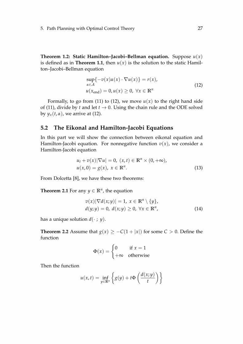
Theorem 1.2: Static Hamilton–Jacobi–Bellman equation. Suppose u(x)is defined as in Theorem 1.1, then u(x) is the solution to the static Hamil-ton–Jacobi–Bellman equation

supα∈A−v(x)α(x) · ∇u(x) = r(x),

u(xend) = 0, u(x) ≥ 0, ∀x ∈ Rn(12)

Formally, to go from (11) to (12), we move u(x) to the right hand sideof (11), divide by t and let t→ 0. Using the chain rule and the ODE solvedby yx(t, α), we arrive at (12).

5.2 The Eikonal and Hamilton-Jacobi Equations

In this part we will show the connection between eikonal equation andHamilton-Jacobi equation. For nonnegative function v(x), we consider aHamilton-Jacobi equation

ut + v(x)|∇u| = 0, (x, t) ∈ Rn × (0,+∞),u(x, 0) = g(x), x ∈ Rn. (13)

From Dolcetta [8], we have these two theorems:

Theorem 2.1 For any y ∈ Rn, the equation

v(x)|∇d(x; y)| = 1, x ∈ Rn \ y,d(y; y) = 0, d(x; y) ≥ 0, ∀x ∈ Rn, (14)

has a unique solution d(· ; y).

Theorem 2.2 Assume that g(x) ≥ −C(1 + |x|) for some C > 0. Define thefunction

Φ(x) =

0 if x = 1+∞ otherwise

Then the function

u(x, t) = infy∈Rn

g(y) + tΦ

(d(x; y)

t

)


is the unique solution of (13) which is bounded below by a function oflinear growth and such that

lim inf(y,t)→(x,0+)

u(y, t) = g(x).

Consider the initial function g(x) = |x − z|, the Euclidean distance to apoint z. By Theorem 2.2, we have that

u(x, t) = infy∈Rn

|y− z|+ tΦ

(d(x; y)

t

)= inf

y∈Rn

d(x;y) = t

|y− z| (15)

is a solution to the equation (13), where d(x; y) is the solution to the eikonalequation (14).

According to (15), u(x, t) = 0 if and only if d(x; z) = t . Thus we deducethe connection between the solution w(x) = d(x; z) to the equation (14)where y = z and the solution u(x, t) to the equation (13):

w(x) = t if and only if u(x, t) = 0.

In this way, any eikonal equation can be transformed into a time-dependentHamilton-Jacobi equation, and vice versa.

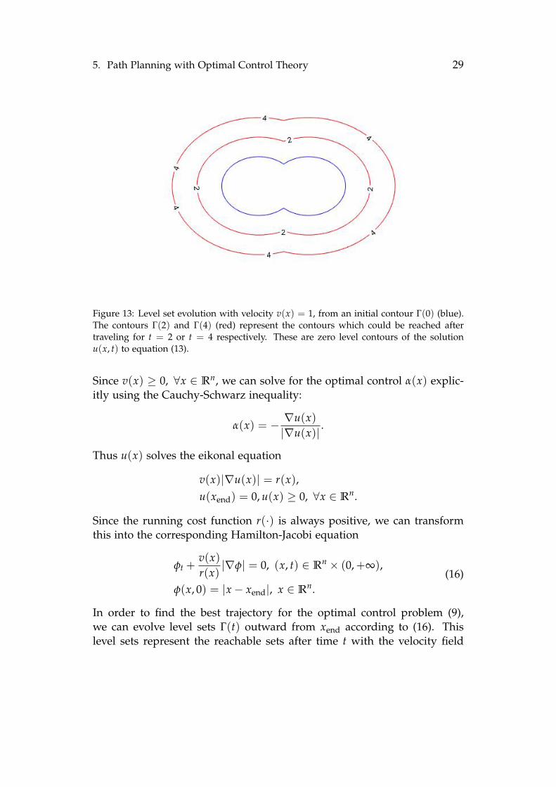
Note that the equation (13) is a level set equation as considered by Osherand Sethian [19]. If g(x) is the signed distance function to a contour Γ(0),we can evolve Γ(0) by level set motion when we solve the PDE. If we defineΓ(t) = x : u(x, t) = 0, then Γ(t) represents the set of points which canbe reached from the original contour with traveling time t in the velocityfield v(x). This is displayed in figure 13. The interpretation of the levelsets Γ(t) as the reachable sets after traveling for time t from an initial stategives a connection between the level set equation and the optimal controlproblem for path planning. In view of the equivalence of (13) and (14),we can obtain the level sets from the solution to either equation; that is,Γ(t) = x : u(x, t) = 0 = x : w(x) = t.

5.3 Finding the Optimal Path

In our model, the optimal control problems have the form (9) where A =α : |α(·)| = 1. If we define the optimal cost u(x) as (10), then u(x)satisfies

supα∈A−v(x)α(x) · ∇u(x) = r(x).


Figure 13: Level set evolution with velocity v(x) = 1, from an initial contour Γ(0) (blue).The contours Γ(2) and Γ(4) (red) represent the contours which could be reached aftertraveling for t = 2 or t = 4 respectively. These are zero level contours of the solutionu(x, t) to equation (13).

Since v(x) ≥ 0, ∀x ∈ Rn, we can solve for the optimal control α(x) explic-itly using the Cauchy-Schwarz inequality:

α(x) = − ∇u(x)|∇u(x)| .

Thus u(x) solves the eikonal equation

v(x)|∇u(x)| = r(x),u(xend) = 0, u(x) ≥ 0, ∀x ∈ Rn.

Since the running cost function r(·) is always positive, we can transformthis into the corresponding Hamilton-Jacobi equation

φt +v(x)r(x)|∇φ| = 0, (x, t) ∈ Rn × (0,+∞),

φ(x, 0) = |x− xend|, x ∈ Rn.(16)

In order to find the best trajectory for the optimal control problem (9),we can evolve level sets Γ(t) outward from xend according to (16). Thislevel sets represent the reachable sets after time t with the velocity field


v(x)/r(x). This time t is no longer traveling time, but rather cost associ-ated with the optimal control problem. Hence the level sets Γ(t) representcontours of equal traveling cost. To find the optimal path from x0 to adesired end point xend. We evolve level sets outward from xend until theyreach x0. That is, we evolve (16) until the time t∗ such that φ(x0, t∗) = 0.This t∗ represents the optimal cost associated with traveling from x0 to xend.

As we solve (16), at each (x, t) we can resolve the optimal control value

α(x, t) = − ∇φ(x, t)|∇φ(x, t)| .

We can use this to resolve the optimal trajectory, by integrating the ODE in(9) backwards from time t = t∗ to t = 0, so that the optimal trajectory isgiven by

x = −v(x)∇φ(x, t)|∇φ(x, t)| ,

x(t∗) = x0.(17)

We should solve the ODE backwards because the function φ(x, t) may notbe differentiable at (xend, 0), and thus we cannot determine the value ofthe optimal control at that point. Note, the optimal trajectory will alwaystravel parallel to ∇φ which is normal to the level sets Γ(t).

In summary, we find the optimal trajectory in two steps:

1. Evolve the level sets. Solve the equation (16) until the time t∗ suchthat φ(x0, t∗) = 0. Here t∗ is the optimal cost in the problem (9).

2. Track back. Solve the dynamic ODE (17) backwards in time, startingfrom x(t∗) = x0. This ODE gives the optimal path we need.

The process of finding an optimal path is displayed in figure 14.

5.4 Optimal Control Problem in Our Model

As described in the previous section, the loggers in our model attempt tosolve the optimization problem

Popt(x, t) ≈ maxXin,Xout

B(x)tT

e−ψ(x)t(

1− β∫ τout

0ψ(Xout(s))ds

)− α(τin + τout)

=B(x)tT

e−ψ(x)t −minXin

∫ τin

0αds

−minXout

∫ τout

0B(x)

tT

e−ψ(x)tβψ(Xout(s)) + αds.


(a) Level set contours (b) Normal directions (c) Optimal path

Figure 14: To find the optimal path from the start point (green dot) to the end point (reddot), we first evolve the level sets from the end point until they reach the start point, andthen let the point travel along the normal direction of the level sets to find the optimalpath.

This formula contains two optimal path planning problems: one is the pathmoving into the forest and the other is the path moving out. Given a startpoint x0 and an end point xend, we need to solve these two optimal controlproblems.The optimal control problem regarding travel into the forest is:

mina∈A

∫ τin

0αds

s.t. Xin = v(Xin)a(Xin)

Xin(0) = x0

τin = inft : Xin(t) = xend.

(18)

The optimal control problem regarding the path moving out of the forestis:

mina∈A

∫ τout

0B(xend)

tT

e−ψ(xend)tβψ(Xout(s)) + αds

s.t. Xout =v(Xout)

1 + c(t/T)γa(Xout)

Xout(0) = xend

τout = inft : Xout(t) = x0.

(19)

The corresponding level set equation for (18) is

φt +v(x)

α|∇φ| = 0, (x, t) ∈ Rn × (0,+∞),

φ(x, 0) = |x− xend|, x ∈ Rn,(20)


and the level set equation for (19) is

φt + vout(x)|∇φ| = 0, (x, t) ∈ Rn × (0,+∞),φ(x, 0) = |x− x0|, x ∈ Rn,

(21)

where

vout(x) =v(x)

(1 + c(t/T)γ)(α + B(xend)tT e−ψ(xend)tβψ(x))

. (22)

We describe the numerical methods for solving these equations in theensuing section.

Note that the denominator of (22) depends on the end point xend. Inour model, for a fixed logging time t and a fixed starting point, we need toevaluate Popt(xend, t) for every possible end point. Theoretically, we need tosolve all these problems over different end points independently and evolvedifferent level set equations for each end point. In order to reduce thecomputational burden, in practice, we discretize B(x) t

T e−ψ(x)t into several

levels. Let bmin = minx

B(x) t

T e−ψ(x)t

and bmax = maxx

B(x) t

T e−ψ(x)t

.We let b0, b1, b2, . . . , bn be a uniform partition of the interval [bmin, bmax].Then grouping the possible ending points into n + 1 collections based onthese values, we only need to evolve n + 1 level set equations with velocitymodified for each of b0, b1, . . . , bn. A similar discretization is employed byArnold et al. [2].

6. Numerical Methods and Implementation 33

6 Numerical Methods and Implementation

In this section, we describe the numerical implementation of the optimalcontrol problem from Section 5. To begin, we discuss the general con-cerns related to numerically solving Hamilton-Jacobi equations, and ad-dress some specific issues related to level set equations.

6.1 Numerical Schemes for Hamilton-Jacobi Equations

Recall, the general Hamilton-Jacobi equation in two spatial dimensions isgiven by

φt + H(φx, φy) = 0,φ(x, 0) = φ0(x).

(23)

In the case of the basic optimal path planning problem, the Hamiltonianwill take the form H(x, y, φx, φy) = v(x, y)

√φ2

x + φ2y; however, we suppress

the dependence of H on x and y to simplify the notation.Because Hamilton-Jacobi equations give rise to solutions with discon-

tinuities in their derivatives, ordinary difference methods, which are per-fectly suitable for advection equations, will often fail to capture the com-plex dynamics at play [6]. Instead, we trade the Hamiltonian H(φx, φy)for the numerical Hamiltonian H(φ+

x , φ−x ; φ+y , φ−y ) which somehow com-

bines the forward difference approximations φ+x , φ+

y and backward differ-ence approximations φ−x , φ−y to the derivatives, in order to more accuratelysimulate the system.

Osher and Shu [18] suggest many choices for the numerical Hamil-tonian, each having its own advantages and disadvantages. Perhaps theeasiest to implement is the Lax-Friedrichs Hamiltonian:

HLF(φ+x , φ−x ; φ+

y , φ−y ) = H

(φ+

x + φ−x2

,φ+

y + φ−y2

)− αx

2(φ+

x − φ−x )−αy

2(φ+

y − φ−y ).

(24)

Here we are adding diffusion to the equation which is on the order of thegrid parameters ∆x, ∆y. The coefficients αx, αy depend on the derivativesof H and determine the amount of diffusion that is added. This numericalHamiltonian has two advantages: first, it is easy to implement, and sec-ond, the added diffusion results in smooth solutions. However, in cases


of optimal path planning, where the motion is driven by a given velocityfield v(x, y), the excessive diffusion can qualitatively change the results,especially near regions of zero velocity [2, 20].

Accordingly, we opt for the minimally diffusive Godunov Hamiltonian:

HG(φ+x , φ−x , φ+

y , φ−y ) = extu∈I(φ−x ,φ+

x )ext

v∈I(φ−y ,φ+y )

H(u, v) (25)

whereI(a, b) = [min(a, b), max(a, b)] (26)

and

extx∈I(a,b)

=

mina≤x≤b if a ≤ b,maxb≤x≤a if a > b.

(27)

These extrema are designed to capture a formal similarity between Hamilton-Jacobi equations and conservation laws, wherein the most important nu-merical consideration is tracking the directions of the characteristics.

The Godunov Hamiltonian can be more difficult to implement, but be-cause it is non-diffusive, it is far preferable for optimal path planning prob-lems. In certain cases, the extrema in (25) can be resolved explicitly. Forexample, when H(φx, φy) = v(x, y)

√φ2

x + φ2y and v ≥ 0, we have

HG(φ+x ,φ−x , φ+

y , φ−y ) =

v(x, y)√

max(φ−x )+, (φ+x )−2 + max(φ−y )+, (φ+

y )−2(28)

where A+ = maxA, 0 and A− = −minA, 0.Having decided on the Godunov Hamiltonian, we simply need to ap-

proximate the derivatives φx, φy and integrate (23) in time. Following Osherand Shu [18], we use the essentially non-oscillatory second order approxi-mations to the spatial derivatives and explicit second order total variationdiminishing Runge-Kutta time stepping to evolve the equation. Specifi-cally, if our discrete domain is given by xi, yj, tk and φk

i,j is our ap-proximation to φ(xi, yj, tk), then our scheme reads

φ∗i,j = φki,j − Hk

i,j∆t,

φk+1i,j =

12

φki,j +

12

φ∗i,j −12

H∗i,j∆t.

where Hk is the Hamiltonian evaluated at φk and H∗ is the Hamiltonianevaluated at φ∗.


Considering our specific case once again, this scheme will be stableand approximate the solution at second order so long as our grid spacingparameters ∆x, ∆y, ∆t satisfy the CFL condition

V∆t(

1∆x

+1

∆y

)< 1

where V = maxx,y v(x, y) [17].

6.2 The Redistancing Problem for Level Set Equations

As discussed in Section 5, the level set equation

φt + v(x)|∇φ| = 0,φ(x, 0) = φ0(x),

(29)

is of particular interest to us. Here the initial function is the signed distancefunction to the initial contour Γ(0) which we desire to evolve via level setmotion. However, when we solve the equation numerically, since the ve-locity function v may be non-smooth, after some steps, there will be someregions where the distortion accumulates and instabilities arise, causingthe level sets Γ(t) = x : φ(x, t) = 0 to become an unreliable measure ofthe points which can be reached by time t. However, because φ is a math-ematical abstraction, and the only quantity we are concerned with is Γ(t),we can circumvent this issue by periodically halting the time integration ofthe equation and replacing φ with the signed distance to the current levelset Γ(t). This is knows as redistancing. It will prevent φ from developinginstabilities, and thus ensure that the level sets Γ(t) are reliable.

There are many ways to accomplish this redistancing. In our algorithm,we use a "crossing time" method. We need to solve the eikonal equation

|∇u| = 1, x ∈ R2

u(x) > 0, x ∈ R2 \Ω,u(x) < 0, x ∈ Ω \ ∂Ω,

where Ω is a closed set in R2. In our case, Ω will represent the interiorof the current level set Γ(t). We consider the Hamilton-Jacobi form of thiseikonal equation,

wt + |∇w| = 0, x ∈ R2, t > 0

w(x, 0) = w0(x), x ∈ R2,(30)


where the initial function w0(x) has zero level set ∂Ω but is not the signeddistance function to ∂Ω as desired. The connection between the Hamilton-Jacobi equation and the eikonal equation is that w(x, t) = 0 if and only ifu(x) = t [8].

We use the first order Godunov scheme and first order time step tosolve the equation (30). First, the zero level-set contour of w(x, t) will beevolved outward from Ω. For each point (xi, yj) outside Ω, when we detectthat the signs of wk

i,j and wk+1i,j are different, we set the signed distance

function u(xi, yj) = (k + 1)∆t. Next, we use the initial function −w0, sothat the zero level-set contour will be evolved inward from Ω. Again foreach (xi, yj) inside Ω, when we detect that wk

i,j and wk+1i,j have different

signs, we set different u(xi, yj) = −(k + 1)∆t.We also implemented several other methods to do the redistancing.

One method based on a Hopf-Lax formulation is suggested by Roystonet al. [22]. Given x ∈ Rn and w satisfying equation (30), we need to solvew(x, t) = 0. This equation can be solved numerically by the secant method,

tk+1 = tk − w(x, tk)tk − tk−1

w(x, tk)− w(x, tk−1),

where the initial t0 and t1 can be chosen from the nearby nodes. Equation(30) can be solved by Hopf-Lax formula,

w(x, t) = miny∈Rn

w(y, 0) + tH∗

(x− y

t

),

where H∗ is the convex conjugate of H. Since H(p) = ‖p‖2, this formulacan be written

w(x, t) = miny∈B(x,t)

w(y, 0)

and this optimization problem can be solved by projected gradient descent.This method has the advantage of being easily parallelizable so that thecomputational complexity will not be influenced too much by the dimen-sion. The disadvantage of this method is that it contains two iterative parts:the secant method to solve the equation φ(x, t) = 0 and projected gradientmethod to find the minimum of φ0(y) in y ∈ B(x, t) and these pieces areembedded in the sense that we must re-solve (29) via the Hopf-Lax for-mula for each iteration tk of the secant method. Since our model is in R2,the calculation burden of those solvers is much greater than that of simply


solving the time-dependent eikonal equation, which is why we opt for theprevious method.

Another method for redistancing, as employed in Arnold et al. [2],Parkinson et al. [20], is to explicitly calculate the distance from each gridpoint to a polygon which approximates the current level set. For eachpoint, the distance to the given polygon is the minimum distance betweenthe point and each edge of the polygon. Thus we must calculate the dis-tance from the point to each edge individually. This computation can beparallelized in both the grid points, and the sides of the polygon. How-ever, in our 2-dimensional model problem, if the size of grid is n× n, thenumber of edges of the polygon will be O(n2) after some time steps, andcalculating the distance between each point and this polygon will have thecomputational complexity O(n4). Empirically, we found this to be muchslower than the crossing time method.

Finally Zhao [24] proposed a fast sweeping method for redistancing.This method is a type of Gauss-Seidel iteration. The strategy is to ’sweep’through the grid from different directions and update the entries in a spe-cific order accordingly. Again, our implementation of this scheme is slowerthan the crossing time method. We also tried to replace the Gauss-Seideliteration here with the Jacobi iteration. Since for an n× n matrix, the Gauss-Seidel iteration needs n steps to update all the entries in this matrix whileJacobi iteration only needs one step. However, the convergence of the Ja-cobi iteration is suspect. One advantage of this method is that it does notrequire the initial function to be a good approximation of the signed dis-tance function; it only requires knowledge of the boundary of Ω. However,in our model problem, when we pause the time integration in order toperform the redistancing, we assume that the function φ(x, t) is a good ap-proximation to the distance function to the current level set Γ(t), and sincethis is true, the fast sweeping method has no advantage over the crossingtime method.

6.3 Implementation Tricks

In order to give a complete account of our numerical methods, we alsodescribe three small implementation tricks that are specific to the problemat hand.

First, when we solve the level set equation numerically, we performredistancing very frequently—roughly every 10 time steps. In order toreduce the computational burden, we only perform the redistancing near


the zero level set contour, then use very simple linear approximation of thedistance on the points which are far away from the zero level set. Sincethe zero level set is the only quantity of interest, and since the level setevolution depends only on the local values of φ(x, t), this will not affectthe quality of the solution. More explicitly, suppose the current level setis Γ(t) and we want to find the signed distance function u(x) to this levelset. Further, assume that Γ(t) is contained in the box [a, b] × [c, d]. If weperform the redistancing every n time steps, then we only need to use thecrossing time method to calculate the distance function for points in therectangle

R = [a− 2n∆x, b + 2n∆x]× [c− 2n∆y, d + 2n∆y].

This is because the crossing time level set is propagating with speed 1, soif it is originally contained in [a, b]× [c, d], then it will remain inside R aftern steps, and further, it will remain unaffected by information propagatinginward from the exterior of R, where we are not perfectly resolving thedistance function. For any point x in the grid but not in R, we take thevalue of the signed distance function u(x) as the boundary value of R plusthe L1 distance between this point and R, namely

u(x) = u(y) + d1(x, y), y = arg miny∈∂R

d1(x, y).

Thus, for example, if (xi, yj) is the top right corner of R, then u(xi+k, yj+`) =u(xi, yj) + k∆x + `∆y.

Second, in implementing crossing time method, we need to evolve equa-tion (30) two times, once outward and once inward. In some cases theinward evolution does not need many steps since the region inside thezero level-set contour will be much smaller than the region outside, dueto the increased velocity along the road and river network in Roraima. Soin practice, if there are some successive steps wherein we don’t detect anysign changes from wk

i,j to wk+1i,j , we assume that the inward evolution is

complete and halt the iteration.Third and finally, as described above, when we perform the redistanc-

ing, the value of u(xi, yj) = (k + 1)∆t when wki,j and wk+1

i,j have a differentsign. However, in reality, the point (xi, yj) could be much closer to k∆t thanit is to (k + 1)∆t. This is especially true of points along the initial contour.These points lie between distances −∆t and ∆t and will be moved fromtheir original location to the midpoint of the contours corresponding to dis-tance −∆t and ∆t, causing the initial contour to be distorted. Accordingly,


rather than explicitly setting u(xi, yj) = (k + 1)∆t, we construct a linearinterpolant wi,j(t) between the values wk

i,j and wk+1i,j and set u(xi, yj) = t0

such that wi,j(t0) = 0.

7. Logging Experiments 40

7 Logging Experiments

In this section we will apply the level set solver to our model as describedin section 6. We give a detailed description of the experimental setup insection 7.1 and analyze the numerical results in section 7.2.

7.1 Experimental Setup

In order to test our model, we first need to prepare data, choose coefficientsand design patrol evaluation metrics.

First, we discuss the calculation of the logging benefit function. weweren’t able to find references on tree category data in the state of Ro-raima. Moreover, neither PRODES nor DETER is a good indicator of log-ging events due to low spatial resolution and other technical issues. Forexample, logging generally will not lead to land clearance, which wouldbe detected by PRODES or DETER. Nevertheless, We decided to constructthe benefit function for logging based on PRODES data. We make the as-sumption that deforestation for farming purpose only takes place within10km of the major highways and treat all the other deforestation events asthe result of logging, which are plotted in figure 15a. We then design thebenefit based on the post-hoc reasoning that high benefit gives rise to highevent frequency within the region. Specifically, we use the same techniqueas in KDE by stamping a 2-D Gaussian to each event. We then generate thelogging benefit by linearly combining the generated density function andthe binary benefit function used in the farming model as is shown in figure15b.

Next, the logging model is much more sensitive to the transportationsystem than the farming model because of the long travel distance to highbenefit regions. We try to design a realistic velocity field, as shown in figure16, to accurately capture the movement of loggers throughout the region.We first get the highway and water map from OpenStreetMap contribu-tors [16]. We assign velocity 1, 0.8, 0.7 to major highways, waterways andsecondary highways respectively. For off highway and off water areas, thevelocity is the average of the vertical and horizontal gradients of each cell,based on a USGS digital elevation model [10].

After this, we need to model the capture intensity. Patrollers’ capture in-tensity is a complicated concept related with patrol resources like availablepatrollers and equipment, patrol strategies like patrol path and frequency,and patrollers’ capture ability. For now, we just deal with the capture in-


(a) Events at least 10km away from high-ways

(b) Benefit constructed for logging

Figure 15: Logging benefit

Figure 16: Velocity field in the state of Roraima

tensity in a simplified and ideal setting, where ψ(x) can be any functionthat fulfills the budget constraint:∫

Ωψ(x)(1 + µd(x))2dx ≤ E

where E is the total budget, d is the Euclidean distance to the major high-ways and µ is a constant. The penalty term (1 + µd(x))2 reflects the factthat it is more expensive to patrol regions far away from highways. In theexperiment, we always set capture intensity so that the constraint reaches


equality, which means the patrollers are always using the entirety of theirbudget.

Among ψ satisfying the budget constraint, we would like to decidewhich patrol strategies are more effective than others. We’ve designedthree different metrics to evaluate patrol efficiency.

• Pristine area ratio PR: we define the regions with non-positive profitas pristine area. PR calculates the ratio of the area of pristine region

over the area of the state as∫

Ω 1P(x)≤0dx∫Ω 1dx .

• Pristine benefit ratio PB: this metric weighs pristine area by benefit

as PB =∫

Ω B(x)1P(x)≤0dx∫Ω B(x)dx and represents the ratio of benefit within the

pristine area over the total benefit.

• Weighted profit WP: as in the farming model, we also interpret thepositive part of the profit as the probability density for loggers tochoose the logging location. We then define WP as the expected profit

by WP =∫

Ω P+(x)2dx∫Ω P+(x)dx , where P+(x) = P(x)1P(x)≥0.

We run the model on a 600 × 600 grid and set time step size to bemin∆x, ∆y/(2 max V) to satisfy the CFL condition, where ∆x and ∆yare the spatial grid size in x and y directions and V is the modified ve-locity in the time-dependent Hamilton-Jacobi equation. We will do a re-initialization every 10 time steps. We set α = µ = 2

(5 maxx∈Ω d(x)) ≈ 7.33×107, β = 1

ln(10) ≈ 4.34× 10−1, T = 2000000.

7.2 Results

We tested our model with different patrol budgets and patrol strategies.We also explored the influence of logging time and changing the velocitywhen traveling with goods. In the end, we will look into optimal loggingpaths and discuss interesting findings.

7.2.1 Example 1: No Patrol

We first impose no patrol. Recall that the returning velocity is modifiedfollowing v(x)/(1+ c(t/T)γ) to take into account the influence of carryingtimber. When the amount of timber has no influence, i.e., c = 0, the optimalpaths traveling in and traveling out are the minimal time path, and the


loggers will always use the maximal logging time T. The resulting profitis shown in figure 17a. We then tested c = 1, γ = 0.5 and γ = 2. Since0 ≤ t/T ≤ 1, γ = 0.5 gives a harsher penalty to velocity than γ = 2, andthus a higher cost. As we can see from figure 17, expected profit is 0 inmost of the region when γ = 0.5. Profit for γ = 2 is only a little bit smallerthan the c = 0 case. In all of the following experiments, we will set c = 0and only look into the influence of patrol.

(a) c = 0 (b) c = 1, γ = 2 (c) c = 1, γ = 0.5

Figure 17: Returning velocity depends on trees obtained, no patrol imposed

7.2.2 Example 2: Comparison of Different Budget

In this example, we set ψ(x) = B(x)E(1+αd(x))11

∫Ω(1+αd(x))−9B(x)dx , which is shown

to be a good patrol strategy in section 7.2.4. We then set E to be 0.001, 0.002and 0.004. The resulting profit is plotted in figure 18. It’s clear that higherbudget will give lower profit. In all of the following experiments, we fix Eto be 0.002.

7.2.3 Example 3: Influence of Patrol on Logging Time

We use the same experimental set up as in the previous example, and wefix E as 0.002. Recall that we discretize the logging time and search for theoptimal time by parameter sweep. In all of the experiments, we discretizelogging time into 10 different levels. We plot the optimal logging time infigure 19a. We then sample 5 points in this region which have optimallogging time 3, 4, 6, 8 and 10 respectively and are marked as red points infigure 19a. Figure 19b shows the profit as a function of logging time ateach point and we see that there are different optimal logging times for


(a) E = 0.001 (b) E = 0.002 (c) E = 0.004

Figure 18: Expected profit with different budget

each point. This is because the risk of capture is higher at some points,making logging for extended periods of time very dangerous.

(a) Optimal time

1 2 3 4 5 6 7 8 9 10

Logging time

-0.4

-0.3

-0.2

-0.1

0

0.1

0.2

Expecte

d p

rofit

Optimal time: 3

Optimal time: 4

Optimal time: 6

Optimal time: 8

Optimal time: 10

(b) Profit changes with logging timeat different spots

Figure 19: Influence of patrol time

7.2.4 Example 4: Comparison of Different Patrol Strategies

In this example, we compare the patrolling efficiency for different cap-ture intensity functions ψ(x). We plot the corresponding capture intensityfunction, profit and optimal time for each experiment and summarize theevaluation based on aforementioned metrics in table 1.


First, we consider a patrol only based on distance to roads by setting

ψ(x) =E

(1 + αd(x))r∫

Ω(1 + αd(x))2−rdx,

where r is chosen to be 1, 3, 7, 11. We may want to give more attentionto regions which are close to roads as logging and patrol costs are low inthese regions. Larger r means the patrol is more concentrated near thehighways, while smaller r leads to more uniformly distributed patrol. Fig-ures 20 - 23 exhibit the corresponding capture intensity, profit and optimaltime. When r = 1, loggers will fully exploit logging time and clear theforest at almost all of the locations, which means capture risk is not a hugethreat. When r increases, the optimal logging time along with the profitnear highways starts to decrease, while profit far away into the forest in-creases. These results give us the clue that we shouldn’t concentrate toomuch along highways. Moreover, all four profit plots have the pattern thathigh benefit regions are high profit regions, which inspire us to take benefitinto consideration.

(a) Capture intensity (b) Profit (c) Optimal time

Figure 20: Patrol based on distance only, r = 1

Next, we set

ψ(x) =B(x)E∫

Ω(1 + αd(x))2B(x)dx

so that the capture intensity is proportional to the benefit. The result isshown in figure 24. Clearly, the intense patrol in high profit regions makethose regions less vulnerable. Figure 24b shows that profitable regions nowcluster around highways where both the initial benefit and the travel cost








is relatively low. The optimal logging time at the northwest corner is muchshorter than in other regions.



Figure 24: Patrol based on benefit only

Previous experiments inform us that we need to balance benefit anddistance when designing a patrol strategy. Here, we set the patrol

ψ(x) =B(x)wE

(1 + αd(x))r∫

Ω(1 + αd(x))2−rB(x)wdx

We tested this patrol with w = 0.5 and 1, r = 3, 7, 11, 15. Results are plottedin figures 25 - 32. Both the figures and table 1 confirm that w = 1, r = 11 isthe best choice.


Figure 25: Patrol based on benefit and distance, w = 1, r = 3

All previous experiments show that both distance to roads and bene-fit are important factors for patrol allocation. For now we do not have amethod to find optimal patrol strategies, but our model can be applied toevaluate and compare different strategies.








7.2.5 Example 5: Optimal Paths

Finally, we calculate the optimal paths that loggers take to and from theirlogging sites. We use the same patrol strategy as shown in figure 30a. We



Figure 29: Patrol based on benefit and distance, w = 0.5, r = 3





sampled 500 points in Roraima based on expected profit and plotted theoptimal path going into the forest (figure 33a) and going out of the forest(figure 33b). We find that the optimal paths that go deeper into the forest




in the northwest corner cluster into one trajectory and the optimal pathsgoing in and going out are quite similar. One reason why this happensis that the capture intensity is much smoother than the velocity field dueto the rivers running across this region. The fast travel speed along theriver outweighs the risk of being captured. Moreover, if we zoom into thenorthwest corner, we can see that the optimal paths for different directionsare not exactly the same because of the influence of patrol.

(a) Optimal path of go-ing into the forest

(b) Optimal path of go-ing out of the forest

(c) Optimal path zoomin

Figure 33: Optimal path


Patrol based on Parameters WP PA PB

Distance only

r = 1 0.2792 0.5674 0.3485r = 3 0.3813 0.5630 0.3302r = 7 0.6192 0.5459 0.2864r = 11 0.8215 0.5237 0.2459

Benefit only 0.1696 0.6820 0.5105

Benefit anddistance

w = 1, r = 3 0.1044 0.6828 0.6805w = 1, r = 7 0.0811 0.7318 0.7394w = 1, r = 11 0.0661 0.7737 0.7883w = 1, r = 15 0.1091 0.7508 0.6115w = 0.5, r = 3 0.1044 0.6828 0.6804w = 0.5, r = 7 0.0856 0.7374 0.6121w = 0.5, r = 11 0.3038 0.7370 0.5569w = 0.5, r = 15 0.6211 0.7232 0.5018

Table 1: Comparison of different patrol strategies

8. Conclusion 52

8 Conclusion

Identifying two modes of deforestation, clearance of land for farming andillegal logging, we build up two mathematical models to describe the ob-served events. To describe land clearance we developed an agent basedmodel for individual farmers who acted as static attackers, clearing moreland with each time step and thus causing more deforestation. For illegallogging, we built a control theoretic model to predict the paths of the log-gers and the locations they may choose to target. Additionally, we detailedthe numerical solvers used for the Hamilton-Jacobi and control theoreticequations. Finally, we tested various patrol strategies with the loggingmodel and the determined which patrol strategies best protected the for-est.

8.1 Farming Model: Main Achievements and Future Work

In our farming model, we constructed the expected profit formula for farm-ers to decide where to clear land for illegal farming. We also performedtime series analysis to simulate the behaviors of farmers and growth offarms, with capture probability built in. We compared our model with realdeforestation data and evaluated the results with average F1 score. Thestrength of our model is that it takes into account many realistic factorssuch as distance to roads, distance to cities, clustering effect, tree coverage,punishment, capture possibility and maximum operation time for farms.Besides this, our model is easy to explain and understand.

In future, we can improve our model by doing some of the following:

• Further optimize our set of parameters.

• Consider more realistic factors.

• Try different patrol strategies and possibly find the optimal one.

• Design a better algorithm to model farm expansion.

8.2 Logging Model: Main Achievements and Future Work

In all previous models, the illegal logging events happen instantaneouslywhen the criminals arrive at the logging location. In our model, we con-sider the logging events occurring over a period of time so that the crimi-nals have a chance of being caught while they are cutting down trees. The

8. Conclusion 53

criminals may not take all the benefit from a spot (i.e. cut down all thetrees in a spot) and they will balance between the chance of getting caughtand the benefit they can gain in order to find a optimal logging time.

We believed this is closer to modeling real life, since we can see onthe satellite map that there are some places where logging events occurredbut trees still remain. With our model, we can evaluate the intensity of alogging event rather than merely decide whether an event will happen ornot.

With different logging times, criminals carry different amount of timberwith them as they travel out of the forest, and the amount of timber willinfluence the velocity. We also calculate the capture probability in a morereasonable way than [2].

Besides this, our model and experiments are based on real data set.The elevation, river, different types of roads and cities are all included inour model, and criminals embark from different cities rather than from theboundary of the region.

In the future, we can do the following to improve our model:

• Remove the linear approximation of capture probability. In our cur-rent logging model, we use a linear approximation of the exponentialterm to make the formula in the optimization problem easier to dealwith. This approximation is not ideal since the exponential term willnever become negative but the linear approximation will. We wouldlike to directly deal with the exponential term in the formula to makeour model more accurate.

• Optimal patrol strategy. Currently we have some metrics to evaluatewhether a patrol strategy is good or not. We use these metrics to com-pare different patrol strategies, but we would like to try to analyticallysolve the optimization problem over the patrol strategy to maximizeor minimize these metrics. Failing this, we would like to design amethod to perturb a given patrol strategy in order to improve it.

• Realistic patrol strategy. Not all the patrol strategies are realistic. Forexample, a patrol strategy that only patrols some spots far inside theforest is not available since most of the policemen live in the citiesand they need to travel along some path from where they live to godeep into the forest. We’d like to solve the following problem: given adesired patrol density, how do we arrange policemen to get a realisticpatrol strategy to approximate the desired one. Here the arrangement

8. Conclusion 54

of policemen includes the traveling path, the velocity, the number ofpoliceman (or the ratio of the number of policemen in each policemangroup to the total number of policemen).

• Improve the model with more real data We suspect that there mightbe some other data which could be included to improve our model.For example, the price of timber, the distribution of different kindsof trees and the population density all likely have significant effectson illegal logging. We don’t have these data now but would like toinclude them in the future.

Bibliography 55

Bibliography

[1] H. J. Albers. Spatial modeling of extraction and enforcement in devel-oping country protected areas. Resource and Energy Economics, 2010.

[2] D. J. Arnold, D. Fernandez, R. Jia, C. Parkinson, D. Tonne, Y. Yaniv,A. L. Bertozzi, and S. J. Osher. Modeling environmental crime in pro-tected areas using the level set method. SIAM Journal on Applied Mathe-matics, 79(3):802–821, 2019. ISSN 0036-1399. doi: 10.1137/18M1205339.

[3] J. J. Assunção, C. Gandour, and R. Rocha. Deforestation slowdown inthe Brazilian Amazon: prices or policies? 2012.

[4] Martino Bardi and Italo Capuzzo-Dolcetta. Optimal control and viscos-ity solutions of Hamilton-Jacobi-Bellman equations. Springer Science &Business Media, 2008.

[5] Elliot Cartee and Alexander Vladimirsky. Control-theoretic models ofenvironmental crime - preprint, 06 2019. URL https://arxiv.org/abs/1906.09289.

[6] M. G. Crandall and P.-L. Lions. Two approximations of solutions ofHamilton-Jacobi equations. Mathematics of Computation, 43(167):1–19,1984.

[7] C. G. Diniz, A. A. d. A. Souza, D. C. Santos, M. C. Dias, N. C. d. Luz,D. R. V. d. Moraes, J. S. Maia, A. R. Gomes, I. d. S. Narvaes, D. M. Va-leriano, L. E. P. Maurano, and M. Adami. DETER-B: The new Amazonnear real-time deforestation detection system. IEEE Journal of SelectedTopics in Applied Earth Observations and Remote Sensing, 8(7):3619–3628,July 2015. ISSN 1939-1404. doi: 10.1109/JSTARS.2015.2437075.

[8] I. C. Dolcetta. The Hopf-Lax solution for state dependent Hamilton-Jacobi equations (viscosity solutions of differential equations and re-lated topics). 2002.

[9] F. Fang, T. H. Nguyen, R. Pickles, W. Y. Lam, G. R. Clements, B. An,A. Singh, B. C. Schwedock, M. Tambe, and A. Lemieux. PAWS — a de-ployed game-theoretic application to combat poaching. AI Magazine,38(1):23–36, Mar. 2017. doi: 10.1609/aimag.v38i1.2710. URL https://www.aaai.org/ojs/index.php/aimagazine/article/view/2710.

https://arxiv.org/abs/1906.09289

https://arxiv.org/abs/1906.09289

https://www.aaai.org/ojs/index.php/aimagazine/article/view/2710

https://www.aaai.org/ojs/index.php/aimagazine/article/view/2710

Bibliography 56

[10] T. G. Farr, P. A. Rosen, E. Caro, R. Crippen, R. Duren, S. Hensley,M. Kobrick, M. Paller, E. Rodriguez, L. Roth, D. Seal, S. Shaffer, J. Shi-mada, J. Umland, M. Werner, M. Oskin, D. Burbank, and D. Als-dorf. The shuttle radar topography mission. Reviews of Geophysics,45(2), 2007. doi: 10.1029/2005RG000183. URL https://agupubs.onlinelibrary.wiley.com/doi/abs/10.1029/2005RG000183.

[11] D. Kar, F. Fang, F. Delle Fave, N. Sintov, and M. Tambe. A game ofthrones: When human behavior models compete in repeated Stackel-berg security games. In Proceedings of the 2015 International Conferenceon Autonomous Agents and Multiagent Systems, pages 1381–1390. Inter-national Foundation for Autonomous Agents and Multiagent Systems,2015.

[12] D. Kar, B. J. Ford, S. Gholami, F. Fang, A. J. Plumptre, M. Tambe,M. Driciru, F. Wanyama, A. Rwetsiba, M. Nsubaga, and J. Mabonga.Cloudy with a chance of poaching: Adversary behavior modeling andforecasting with real-world poaching data. In AAMAS, 2017.

[13] W. F. Laurance, A. K. M. Albernaz, G. Schroth, P. M. Fearn-side, S. Bergen, E. M. Venticinque, and C. Da Costa. Predic-tors of deforestation in the Brazilian Amazon. Journal of Bio-geography, 29(5-6):737–748, 2002. doi: 10.1046/j.1365-2699.2002.00721.x. URL https://onlinelibrary.wiley.com/doi/abs/10.1046/j.1365-2699.2002.00721.x.

[14] G. O. Mohler, A. L. Bertozzi, T. A. Goldstein, and S. J. Osher. FastTV regularization for 2D maximum penalized likelihood estimation.Journal of Computational and Graphical Statistics, 20(2):479–491, 2011.

[15] National Institute of Space Research (INPE). PRODES de-forestation. Accessed through Global Forest Watch in 07/2019.www.globalforestwatch.org.

[16] OpenStreetMap contributors. Planet dump retrieved fromhttps://planet.osm.org . https://www.openstreetmap.org, 2017.

[17] S. J. Osher and R. P. Fedkiw. Level Set Methods and Dynamic ImplicitSurfaces. Springer Verlag, 2003.

https://agupubs.onlinelibrary.wiley.com/doi/abs/10.1029/2005RG000183

https://agupubs.onlinelibrary.wiley.com/doi/abs/10.1029/2005RG000183

https://onlinelibrary.wiley.com/doi/abs/10.1046/j.1365-2699.2002.00721.x

https://onlinelibrary.wiley.com/doi/abs/10.1046/j.1365-2699.2002.00721.x

https://www.openstreetmap.org

Bibliography 57

[18] S. J. Osher and C.-W. Shu. High order essentially non-oscillatoryschemes for Hamilton-Jacobi equations. SIAM Journal of NumericalAnalysis, 28(4):907–922, 1991.

[19] Stanley Osher and James Sethian. Fronts propagating with curvaturedependent speed: Algorithms based on Hamilton-Jacobi formulations.Journal of Computational Physics, 79:12–49, 1988.

[20] C. Parkinson, D. J. Arnold, A. L. Bertozzi, Y. T. Chow, and S. J. Os-her. Optimal human navigation in steep terrain: a Hamilton-Jacobi-Bellman approach. Communications in Mathematical Sciences, 17:227–242, 01 2019. doi: 10.4310/CMS.2019.v17.n1.a9.

[21] A. S. P. Pfaff. What drives deforestation in the Brazilian Amazon?:Evidence from satellite and socioeconomic data. Journal of Environ-mental Economics and Management, 37(1):26 – 43, 1999. ISSN 0095-0696. doi: https://doi.org/10.1006/jeem.1998.1056. URL http://www.sciencedirect.com/science/article/pii/S0095069698910567.

[22] M. Royston, A. Pradhana, B. Lee, Y. T. Chow, W. Yin, J. Teran, and S. J.Osher. Parallel redistancing using the Hopf–Lax formula. Journal ofComputational Physics, 365:7–17, 2018.

[23] T. Slough, J. Urpelainen, and Johns Hopkins SAIS. Public policy un-der limited state capacity: Evidence from deforestation control in theBrazilian Amazon. Technical report, mimeo, 2018.

[24] H. Zhao. A fast sweeping method for eikonal equations. Mathematicsof computation, 74(250):603–627, 2005.

http://www.sciencedirect.com/science/article/pii/S0095069698910567

http://www.sciencedirect.com/science/article/pii/S0095069698910567

mathematical models of deforestation in the brazilian

Documents