mean-variance portfolio optimization when means and

The Annals of Applied Statistics2011, Vol. 5, No. 2A, 798–823DOI: 10.1214/10-AOAS422© Institute of Mathematical Statistics, 2011

MEAN–VARIANCE PORTFOLIO OPTIMIZATION WHEN MEANSAND COVARIANCES ARE UNKNOWN1

BY TZE LEUNG LAI, HAIPENG XING AND ZEHAO CHEN

Stanford University, SUNY at Stony Brook and Bosera Fund

Markowitz’s celebrated mean–variance portfolio optimization theory as-sumes that the means and covariances of the underlying asset returns areknown. In practice, they are unknown and have to be estimated from histori-cal data. Plugging the estimates into the efficient frontier that assumes knownparameters has led to portfolios that may perform poorly and have counter-intuitive asset allocation weights; this has been referred to as the “Markowitzoptimization enigma.” After reviewing different approaches in the literatureto address these difficulties, we explain the root cause of the enigma and pro-pose a new approach to resolve it. Not only is the new approach shown toprovide substantial improvements over previous methods, but it also allowsflexible modeling to incorporate dynamic features and fundamental analysisof the training sample of historical data, as illustrated in simulation and em-pirical studies.

1. Introduction. The mean–variance (MV) portfolio optimization theory ofHarry Markowitz (1952, 1959), Nobel laureate in economics, is widely regardedas one of the foundational theories in financial economics. It is a single-period the-ory on the choice of portfolio weights that provide the optimal tradeoff betweenthe mean (as a measure of profit) and the variance (as a measure of risk) of theportfolio return for a future period. The theory, which will be briefly reviewed inthe next paragraph, assumes that the means and covariances of the underlying as-set returns are known. How to implement the theory in practice when the meansand covariances are unknown parameters has been an intriguing statistical prob-lem in financial economics. This paper proposes a novel approach to resolve thelong-standing problem and illustrates it with an empirical study using CRSP (theCenter for Research in Security Prices of the University of Chicago) monthly stockprice data, which can be accessed via the Wharton Research Data Services at theUniversity of Pennsylvania.

For a portfolio consisting of m assets (e.g., stocks) with expected returns μi , letwi be the weight of the portfolio’s value invested in asset i such that

∑mi=1 wi = 1,

and let w = (w1, . . . ,wm)T , μ = (μ1, . . . ,μm)T , 1 = (1, . . . ,1)T . The portfolio

Received May 2009; revised September 2010.1Supported by NSF Grants DMS-08-05879 at Stanford University and DMS-09-06593 at SUNY,

Stony Brook.Key words and phrases. Markowitz’s portfolio theory, efficient frontier, empirical Bayes, stochas-

tic optimization.

798

http://www.imstat.org/aoas/

http://dx.doi.org/10.1214/10-AOAS422

http://www.imstat.org

MEAN–VARIANCE PORTFOLIO OPTIMIZATION 799

return has mean wT μ and variance wT �w, where � is the covariance matrix ofthe asset returns; see Lai and Xing (2008), pages 67, 69–71. Given a target valueμ∗ for the mean return of a portfolio, Markowitz characterizes an efficient portfolioby its weight vector weff that solves the optimization problem

weff = arg minw

wT �w subject to wT μ = μ∗,wT 1 = 1,w ≥ 0.(1.1)

When short selling is allowed, the constraint w ≥ 0 (i.e., wi ≥ 0 for all i) in (1.1)can be removed, yielding the following problem that has an explicit solution:

weff = arg minw:wT μ=μ∗, wT 1=1

wT �w

(1.2)= {B�−11 − A�−1μ + μ∗(C�−1μ − A�−11)}/D,

where A = μT �−11 = 1T �−1μ,B = μT �−1μ,C = 1T �−11, and D =BC − A2.

Markowitz’s theory assumes known μ and �. Since in practice μ and � areunknown, a commonly used approach is to estimate μ and � from historical data,under the assumption that returns are i.i.d. A standard model for the price Pit ofthe ith asset at time t in finance theory is geometric Brownian motion dPit/Pit =θi dt + σi dB

(i)t , where {B(i)

t , t ≥ 0} is standard Brownian motion. The discrete-time analog of this price process has returns rit = (Pit − Pi,t−1)/Pi,t−1, and logreturns log(Pit/Pi,t−1) = log(1 + rit ) ≈ rit that are i.i.d. N(θi − σ 2

i /2, σ 2i ). Under

the standard model, maximum likelihood estimates of μ and � are the samplemean μ and the sample covariance matrix �, which are also method-of-momentsestimates without the assumption of normality and when the i.i.d. assumption isreplaced by weak stationarity (i.e., time-invariant means and covariances). It hasbeen found, however, that replacing μ and � in (1.1) or (1.2) by their samplecounterparts μ and � may perform poorly and a major direction in the literatureis to find other (e.g., Bayes and shrinkage) estimators that yield better portfolioswhen they are plugged into (1.1) or (1.2). An alternative method, introduced byMichaud (1989) to tackle the “Markowitz optimization enigma,” is to adjust theplug-in portfolio weights by incorporating sampling variability of (μ, �) via thebootstrap. Section 2 gives a brief survey of these approaches.

Let rt = (r1t , . . . , rmt )T . Since Markowitz’s theory deals with portfolio returns

in a future period, it is more appropriate to use the conditional mean and covari-ance matrix of the future returns rn+1 given the historical data rn, rn−1, . . . basedon a Bayesian model that forecasts the future from the available data, rather thanrestricting to an i.i.d. model that relates the future to the past via the unknownparameters μ and � for future returns to be estimated from past data. More im-portantly, this Bayesian formulation paves the way for a new approach that gen-eralizes Markowitz’s portfolio theory to the case where the means and covari-ances are unknown. When μ and � are estimated from data, their uncertaintiesshould be incorporated into the risk; moreover, it is not possible to attain a target

800 T. L. LAI, H. XING AND Z. CHEN

level of mean return as in Markowitz’s constraint wT μ = μ∗ since μ is unknown.To address this root cause of the Markowitz enigma, we introduce in Section 3a Bayesian approach that assumes a prior distribution for (μ,�) and formulatesmean–variance portfolio optimization as a stochastic optimization problem. Thisoptimization problem reduces to that of Markowitz when the prior distribution isdegenerate. It uses the posterior distribution given current and past observationsto incorporate the uncertainties of μ and � into the variance of the portfolio re-turn wT rn+1, where w is based on the posterior distribution. The constraint inMarkowitz’s mean–variance formulation can be included in the objective functionby using a Lagrange multiplier λ−1 so that the optimization problem is to evalu-ate the weight vector w that maximizes E(wT rn+1) − λVar(wT rn+1), for whichλ can be regarded as a risk aversion coefficient. To compare with previous fre-quentist approaches that assume i.i.d. returns, Section 4 introduces a variant of theBayes rule that uses bootstrap resampling to estimate the performance criterionnonparametrically.

To apply this theory in practice, the investor has to figure out his/her risk aver-sion coefficient, which may be a difficult task. Markowitz’s theory circumventsthis by considering the efficient frontier, which is the (σ,μ) curve of efficient port-folios as λ varies over all possible values, where μ is the mean and σ 2 the varianceof the portfolio return. Investors, however, often prefer to use (μ − μ0)/σe, calledthe information ratio, as a measure of a portfolio’s performance, where μ0 is theexpected return of a benchmark investment and σ 2

e is the variance of the portfo-lio’s excess return over the benchmark portfolio; see Grinold and Kahn (2000),page 5. The benchmark investment can be a market portfolio (e.g., S&P500) orsome other reference portfolio, or a risk-free bank account with interest rate μ0(in which case the information ratio is often called the Sharpe ratio). Note that theinformation ratio is proportional to μ − μ0 and inversely proportional to σe, andcan be regarded as the excess return per unit of risk. In Section 5 we describe howλ can be chosen for the rule developed in Section 3 to maximize the informationratio. Other statistical issues that arise in practice are also considered in Sections 5and 6 where they lead to certain modifications of the basic rule. Among them aredimension reduction when m (number of assets) is not small relative to n (numberof past periods in the training sample) and departures of the historical data fromthe working assumption of i.i.d. asset returns. Section 6 illustrates these methodsin an empirical study in which the rule thus obtained is compared with other rulesproposed in the literature. Some concluding remarks are given in Section 7.

2. Using better estimates of μ, � or weff to implement Markowitz’s port-folio optimization theory. Since μ and � in Markowitz’s efficient frontier areactually unknown, a natural idea is to replace them by the sample mean vectorμ and covariance matrix � of the training sample. However, this plug-in fron-tier is no longer optimal because μ and � actually differ from μ and �, and


Frankfurter, Phillips and Seagle (1976) and Jobson and Korkie (1980) have re-ported that portfolios associated with the plug-in frontier can perform worse thanan equally weighted portfolio that is highly inefficient. Michaud (1989) commentsthat the minimum variance (MV) portfolio weff based on μ and � has seriousdeficiencies, calling the MV optimizers “estimation-error maximizers.” His argu-ment is reinforced by subsequent studies, for example, Best and Grauer (1991),Chopra, Hensel and Turner (1993), Canner et al. (1997), Simann (1997) andBritten-Jones (1999). Three approaches have emerged to address the difficulty dur-ing the past two decades. The first approach uses multifactor models to reduce thedimension in estimating �, and the second approach uses Bayes or other shrinkageestimates of �. Both approaches use improved estimates of � for the plug-in ef-ficient frontier. They have also been modified to provide better estimates of μ, forexample, in the quasi-Bayesian approach of Black and Litterman (1990). The thirdapproach uses bootstrapping to correct for the bias of weff as an estimate of weff.

2.1. Multifactor pricing models. Multifactor pricing models relate the m assetreturns ri to k factors f1, . . . , fk in a regression model of the form

ri = αi + (f1, . . . , fk)T βi + εi,(2.1)

in which αi and β i are unknown regression parameters and εi is an unobserved ran-dom disturbance that has mean 0 and is uncorrelated with f := (f1, . . . , fk)

T . Thecase k = 1 is called a single-factor (or single-index) model. Under Sharpe’s (1964)capital asset pricing model (CAPM) which assumes, besides known μ and �, thatthe market has a risk-free asset with return rf (interest rate) and that all investorsminimize the variance of their portfolios for their target mean returns, (2.1) holdswith k = 1, αi = rf and f = rM − rf , where rM is the return of a hypotheticalmarket portfolio M which can be approximated in practice by an index fund suchas Standard and Poor’s (S&P) 500 Index. The arbitrage pricing theory (APT), in-troduced by Ross (1976), involves neither a market portfolio nor a risk-free assetand states that a multifactor model of the form (2.1) should hold approximatelyin the absence of arbitrage for sufficiently large m. The theory, however, does notspecify the factors and their number. Methods for choosing factors in (2.1) canbe broadly classified as economic and statistical, and commonly used statisticalmethods include factor analysis and principal component analysis; see Section 3.4of Lai and Xing (2008).

2.2. Bayes and shrinkage estimators. A popular conjugate family of prior dis-tributions for estimation of covariance matrices from i.i.d. normal random vec-tors rt with mean μ and covariance matrix � is

μ|� ∼ N(ν,�/κ), � ∼ IWm(�, n0),(2.2)


where IWm(�, n0) denotes the inverted Wishart distribution with n0 degrees offreedom and mean �/(n0 − m − 1). The posterior distribution of (μ,�) given(r1, . . . , rn) is also of the same form:

μ|� ∼ N(μ,�/(n + κ)

), � ∼ IWm

((n + n0 − m − 1)�, n + n0

),

where μ and � are the Bayes estimators of μ and � given by

μ = κ

n + κν + n

n + κr,

� = n0 − m − 1

n + n0 − m − 1

�

n0 − m − 1(2.3)

+ n

n + n0 − m − 1

{1

n

n∑i=1

(rt − r)(rt − r)T

+ κ

n + κ(r − ν)(r − ν)T

}.

Note that the Bayes estimator � adds to the MLE of � the covariance matrixκ(r − ν)(r − ν)T /(n + κ), which accounts for the uncertainties due to replacingμ by r, besides shrinking this adjusted covariance matrix toward the prior mean�/(n0 − m − 1).

Simply using r to estimate μ, Ledoit and Wolf (2003, 2004) propose to shrinkthe MLE of � toward a structured covariance matrix, instead of using directlythis Bayes estimator which requires specification of the hyperparameters μ, κ , n0and � . Their rationale is that whereas the MLE S = ∑n

t=1(rt − r)(rt − r)T /n

has a large estimation error when m(m + 1)/2 is comparable with n, a structuredcovariance matrix F has much fewer parameters that can be estimated with smallervariances. They propose to estimate � by a convex combination of F and S:

� = δF + (1 − δ)S,(2.4)

where δ is an estimator of the optimal shrinkage constant δ used to shrink the MLEtoward the estimated structured covariance matrix F. Besides the covariance ma-trix F associated with a single-factor model, they also suggest using a constant cor-relation model for F in which all pairwise correlations are identical, and have foundthat it gives comparable performance in simulation and empirical studies. Theyadvocate using this shrinkage estimate in lieu of S in implementing Markowitz’sefficient frontier.

The difficulty of estimating μ well enough for the plug-in portfolio to havereliable performance was pointed out by Black and Litterman (1990), who pro-posed the following pragmatic quasi-Bayesian approach to address this difficulty.Whereas Jorion (1986) had used earlier a shrinkage estimator similar to μ in (2.3),which can be viewed as shrinking a prior mean ν to the sample mean r (instead


of the other way around), Black and Litterman’s approach basically amountedto shrinking an investor’s subjective estimate of μ to the market’s estimate im-plied by an “equilibrium portfolio.” The investor’s subjective guess of μ is de-scribed in terms of “views” on linear combinations of asset returns, which canbe based on past observations and the investor’s personal/expert opinions. Theseviews are represented by Pμ ∼ N(q,�), where P is a p × m matrix of the in-vestor’s “picks” of the assets to express the guesses, and � is a diagonal matrix thatexpresses the investor’s uncertainties in the views via their variances. The “equi-librium portfolio,” denoted by w, is based on a normative theory of an equilibriummarket, in which w is assumed to solve the mean–variance optimization problemmaxw(wT π − λwT �w), with λ being the average risk-aversion level of the mar-ket and π representing the market’s view of μ. This theory yields the relationπ = 2λ�w, which can be used to infer π from the market capitalization or bench-mark portfolio as a surrogate of w. Incorporating uncertainty in the market’s viewof μ, Black and Litterman assume that π − μ ∼ N(0, τ�), in which τ ∈ (0,1)

is a small parameter, and also set exogenously λ = 1.2; see Meucci (2010). Com-bining Pμ ∼ N(q,�) with π − μ ∼ N(0, τ�) under a working independenceassumption between the two multivariate normal distributions yields the Black–Litterman estimate of μ:

μBL = [(τ�)−1 + PT �−1P]−1[(τ�)−1π + PT �−1q],(2.5)

with covariance matrix [(τ�)−1 + PT �−1P]−1. Various modifications and exten-sions of their idea have been proposed; see Meucci (2005), pages 426–437, Fabozziet al. (2007), pages 232–253, and Meucci (2010). These extensions have the basicform (2.5) or some variant thereof, and differ mainly in the normative model usedto generate an equilibrium portfolio. Note that (2.5) involves �, which Black andLitterman estimated by using the sample covariance matrix of historical data, andthat their focus was to address the estimation of μ for the plug-in portfolio. ClearlyBayes or shrinkage estimates of � can be used instead.

2.3. Bootstrapping and the resampled frontier. To adjust for the bias of weffas an estimate of weff, Michaud (1989) uses the average of the bootstrap weightvectors:

w = B−1B∑

b=1

w∗b,(2.6)

where w∗b is the estimated optimal portfolio weight vector based on the bth boot-

strap sample {r∗b1, . . . , r∗

bn} drawn with replacement from the observed sample{r1, . . . , rn}. Specifically, the bth bootstrap sample has sample mean vector μ∗

b

and covariance matrix �∗b, which can be used to replace μ and � in (1.1) or (1.2),

thereby yielding w∗b. Thus, the resampled efficient frontier corresponds to plotting

wT μ versus√

wT �w for a fine grid of μ∗ values, where w is defined by (2.6) inwhich w∗

b depends on the target level μ∗.


3. A stochastic optimization approach. The Bayesian and shrinkage meth-ods in Section 2.2 focus primarily on Bayes estimates of μ and � (with normaland inverted Wishart priors) and shrinkage estimators of �. However, the con-struction of efficient portfolios when μ and � are unknown is more complicatedthan trying to estimate them as well as possible and then plugging the estimatesinto (1.1) or (1.2). Note in this connection that (1.2) involves �−1 instead of � andthat estimating � as well as possible does not imply that �−1 is reliably estimated.Estimation of a high-dimensional m × m covariance matrix and its inverse whenm2 is not small compared to n has been recognized as a difficult statistical prob-lem and attracted much recent attention; see, for example, Ledoit and Wolf (2004),Huang et al. (2006), Bickel and Lavina (2008) and Fan, Fan and Lv (2008). Somesparsity condition or a low-dimensional factor structure is needed to obtain an esti-mate which is close to � and whose inverse is close to �−1, but the conjugate priorfamily (2.2) that motivates the (linear) shrinkage estimators (2.3) or (2.4) does notreflect such sparsity. For high-dimensional weight vectors weff, direct applicationof the bootstrap for bias correction is also problematic.

A major difficulty with the “plug-in” efficient frontier (which uses S to esti-mate � and r to estimate μ), its variants that estimate � by (2.4) and μ by (2.3)or the Black–Litterman method, and its “resampled” version is that Markowitz’sidea of using the variance of wT rn+1 as a measure of the portfolio’s risk cannotbe captured simply by the plug-in estimates wT �w of Var(wT rn+1) and wT μ

of E(wT rn+1). This difficulty was recognized by Broadie (1993), who used theterms true frontier and estimated frontier to refer to Markowitz’s efficient fron-tier (with known μ and �) and the plug-in efficient frontier, respectively, and whoalso suggested considering the actual mean and variance of the return of an esti-mated frontier portfolio. Whereas the problem of minimizing Var(wT rn+1) subjectto a given level μ∗ of the mean return E(wT rn+1) is meaningful in Markowitz’sframework, in which both E(rn+1) and Cov(rn+1) are known, the surrogate prob-lem of minimizing wT �w under the constraint wT μ = μ∗ ignores the fact thatboth μ and � have inherent errors (risks) themselves. In this section we considerthe more fundamental problem

max{E(wT rn+1) − λVar(wT rn+1)}(3.1)

when μ and � are unknown and treated as state variables whose uncertaintiesare specified by their posterior distributions given the observations r1, . . . , rn ina Bayesian framework. The weights w in (3.1) are random vectors that depend onr1, . . . , rn. Note that if the prior distribution puts all its mass at (μ0,�0), then theminimization problem (3.1) reduces to Markowitz’s portfolio optimization prob-lem that assumes μ0 and �0 are given. The Lagrange multiplier λ in (3.1) can beregarded as the investor’s risk-aversion index when variance is used to measurerisk.


3.1. Solution of the optimization problem (3.1). The problem (3.1) is nota standard stochastic optimization problem because of the term [E(wT rn+1)]2

in Var(wT rn+1) = E[(wT rn+1)2] − [E(wT rn+1)]2. A standard stochastic opti-

mization problem in the Bayesian setting is of the form maxa∈A Eg(X, θ, a),in which g(X, θ, a) is the reward when action a is taken, X is a random vec-tor with distribution Fθ , θ has a prior distribution and the maximization is overthe action space A. The key to its solution is the law of conditional expecta-tions Eg(X, θ, a) = E{E[g(X, θ , a)|X]}, which implies that the stochastic op-timization problem can be solved by choosing a to maximize the posterior re-ward E[g(X, θ, a)|X]}. This key idea, however, cannot be applied to the prob-lem of maximizing or minimizing nonlinear functions of Eg(X, θ, a), such as[Eg(X, θ, a)]2 that is involved in (3.1).

Our method of solving (3.1) is to convert it to a standard stochastic controlproblem by using an additional parameter. Let W = wT rn+1 and note that E(W)−λVar(W) = h(EW,EW 2), where h(x, y) = x +λx2 −λy. Let WB = wT

Brn+1 andη = 1 + 2λE(WB), where wB is the Bayes weight vector. Then

0 ≥ h(EW,EW 2) − h(EWB,EW 2B)

= E(W) − E(WB) − λ{E(W 2) − E(W 2B)} + λ{(EW)2 − (EWB)2}

= η{E(W) − E(WB)} + λ{E(W 2B) − E(W 2)} + λ{E(W) − E(WB)}2

≥ {λE(W 2B) − ηE(WB)} − {λE(W 2) − ηE(W)}.

Moreover, the last inequality is strict unless EW = EWB , in which case the firstinequality is strict unless EW 2 = EW 2

B . This shows that the last term above is ≤0or, equivalently,

λE(W 2) − ηE(W) ≥ λE(W 2B) − ηE(WB),(3.2)

and that equality holds in (3.2) if and only if W has the same mean and varianceas WB . Hence, the stochastic optimization problem (3.1) is equivalent to mini-mizing λE[(wT rn+1)

2] − ηE(wT rn+1) over weight vectors w that can depend onr1, . . . , rn. Since η = 1 + 2λE(WB) is a linear function of the solution of (3.1), wecannot apply this equivalence directly to the unknown η. Instead we solve a familyof standard stochastic optimization problems over η and then choose the η thatmaximizes the reward in (3.1).

To summarize, we can solve (3.1) by rewriting it as the following maximizationproblem over η:

maxη

{E[wT (η)rn+1] − λVar[wT (η)rn+1]},(3.3)

where w(η) is the solution of the stochastic optimization problem

w(η) = arg minw

{λE[(wT rn+1)2] − ηE(wT rn+1)}.


3.2. Computation of the optimal weight vector. Let μn and Vn be the pos-terior mean and second moment matrix given the set Rn of current and past re-turns r1, . . . , rn. Since w is based on Rn, it follows from E(rn+1|Rn) = μn andE(rn+1rT

n+1|Rn) = Vn that

E(wT rn+1) = E(wT μn), E[(wT rn+1)2] = E(wT Vnw).(3.4)

Without short selling, the weight vector w(η) in (3.3) is given by the followinganalog of (1.1):

w(η) = arg minw:wT 1=1,w≥0

{λwT Vnw − ηwT μn},(3.5)

which can be computed by quadratic programming (e.g., by quadprog inMATLAB). When short selling is allowed but there are limits on short setting, theconstraint w ≥ 0 can be replaced by w ≥ w0, where w0 is a vector of negativenumbers. When there is no limit on short selling, the constraint w ≥ 0 in (3.5) canbe removed and w(η) in (3.3) is given explicitly by

w(η) = arg minw:wT 1=1

{λwT Vnw − ηwT μn}(3.6)

= 1

Cn

V−1n 1 + η

2λV−1

n

(μn − An

Cn

1),

where the second equality can be derived by using a Lagrange multiplier and

An = μTn V−1

n 1 = 1T V−1n μn, Bn = μT

n V−1n μn, Cn = 1T V−1

n 1.(3.7)

Quadratic programming can be used to compute w(η) for more general linear andquadratic constraints than those in (3.5); see Fabozzi et al. (2007), pages 88–92.

Note that (3.5) or (3.6) essentially plugs the Bayes estimates of μ and V :=� + μμT into the optimal weight vector that assumes μ and � to be known.However, unlike the “plug-in” efficient frontier described in the first paragraphof Section 2, we have first transformed the original mean–variance portfolio opti-mization problem into a “mean versus second moment” optimization problem thathas an additional parameter η. Putting (3.5) or (3.6) into

C(η) := E[wT (η)μn] + λ(E[wT (η)μn])2 − λE[wT (η)Vnw(η)],(3.8)

which is equal to E[wT (η)r]−λVar[wT (η)r] by (3.4), we can use Brent’s method[Press et al. (1992), pages 359–362] to maximize C(η). It should be noted that thisargument implicitly assumes that the maximum of (3.1) is attained by some wand is finite. Whereas this assumption is satisfied when there are limits on shortselling as in (3.5), it may not hold when there is no limit on short selling. In fact,the explicit formula of w(η) in (3.6) can be used to express (3.8) as a quadraticfunction of η:

C(η) = η2

4λE

{(Bn − A2

n

Cn

)(Bn − A2

n

Cn

− 1)}

+ ηE

{(1

2λ+ An

Cn

)(Bn − A2

n

Cn

)}

+ E

{An

Cn

+ λA2

n − Cn

C2n

},


which has a maximum only if

E

{(Bn − A2

n

Cn

)(Bn − A2

n

Cn

− 1)}

< 0.(3.9)

In the case E{(Bn − A2n

Cn)(Bn − A2

n

Cn− 1)} > 0, C(η) has a minimum instead and

approaches to ∞ as |η| → ∞. In this case, (3.1) has an infinite value and shouldbe defined as a supremum (which is not attained) instead of a maximum.

REMARK. Let �n denote the posterior covariance matrix given Rn. Note thatthe law of iterated conditional expectations, from which (3.4) follows, has the fol-lowing analog for Var(W):

Var(W) = E[Var(W |Rn)] + Var[E(W |Rn)](3.10)

= E(wT �nw) + Var(wT μn).

Using �n to replace � in the optimal weight vector that assumes μ and � to beknown, therefore, ignores the variance of wT μn in (3.10), and this omission is animportant root cause for the Markowitz optimization enigma related to “plug-in”efficient frontiers.

4. Empirical Bayes, bootstrap approximation and frequentist risk. Formore flexible modeling, one can allow the prior distribution in the precedingBayesian approach to include unspecified hyperparameters, which can be esti-mated from the training sample by maximum likelihood, or method of momentsor other methods. For example, for the conjugate prior (2.2), we can assume ν and� to be functions of certain hyperparameters that are associated with a multifac-tor model of the type (2.1). This amounts to using an empirical Bayes model for(μ,�) in the stochastic optimization problem (3.1). Besides a prior distributionfor (μ,�), (3.1) also requires specification of the common distribution of the i.i.d.returns to evaluate Eμ,�(wT rn+1) and Varμ,�(wT rn+1). The bootstrap providesa nonparametric method to evaluate these quantities, as described below.

4.1. Bootstrap estimate of performance. To begin with, note that we canevaluate the frequentist performance of asset allocation rules by making use ofthe bootstrap method. The bootstrap samples {r∗

b1, . . . , r∗bn} drawn with replace-

ment from the observed sample {r1, . . . , rn}, 1 ≤ b ≤ B , can be used to esti-mate its Eμ,�(wT

n rn+1) = Eμ,�(wTn μ) and Varμ,�(wT

n rn+1) = Eμ,�(wTn �wn) +

Varμ,�(wTn μ) of various portfolios � whose weight vectors wn may depend

on r1, . . . , rn. In particular, we can use Bayes or other estimators for μn andVn in (3.5) or (3.6) and then choose η to maximize the bootstrap estimate ofEμ,�(wT

n rn+1) − λVarμ,�(wTn rn+1). This is tantamount to using the empirical

distribution of r1, . . . , rn to be the common distribution of the returns. In particu-lar, using r for μn in (3.5) and the second moment matrix n−1 ∑n

t=1 rtrTt for Vn

in (3.6) provides a “nonparametric empirical Bayes” variant, abbreviated by NPEBhereafter, of the optimal rule in Section 3.


4.2. A simulation study of Bayes and frequentist rewards. The following sim-ulation study assumes i.i.d. annual returns (in %) of m = 4 assets whose meanvector and covariance matrix are generated from the normal and inverted Wishartprior distribution (2.2) with κ = 5, n0 = 10, ν = (2.48,2.17,1.61,3.42)T and thehyperparameter � given by

�11 = 3.37, �22 = 4.22, �33 = 2.75, �44 = 8.43,

�12 = 2.04,

�13 = 0.32, �14 = 1.59, �23 = −0.05,

�24 = 3.02, �34 = 1.08.

We consider four scenarios for the case n = 6 without short selling. The first sce-nario assumes this prior distribution and studies the Bayesian reward for λ = 1,5and 10. The other scenarios consider the frequentist reward at three values of(μ,�) generated from the prior distribution. These values, denoted by Freq 1,Freq 2, Freq 3, are as follows:

Freq 1: μ = (2.42,1.88,1.58,3.47)T , �11 = 1.17,�22 = 0.82,�33 = 1.37,

�44 = 2.86,�12 = 0.79,�13 = 0.84,�14 = 1.61,�23 = 0.61,�24 = 1.23,�34 =1.35.

Freq 2: μ = (2.59,2.29,1.25,3.13)T , �11 = 1.32,�22 = 0.67,�33 = 1.43,

�44 = 1.03,�12 = 0.75,�13 = 0.85,�14 = 0.68,�23 = 0.32,�24 = 0.44,�34 =0.61.

Freq 3: μ = (1.91,1.58,1.03,2.76)T , �11 = 1.00,�22 = 0.83,�33 = 0.35,

�44 = 0.62,�12 = 0.73,�13 = 0.26,�14 = 0.36,�23 = 0.16,�24 = 0.50,�34 =0.14.

Table 1 compares the Bayes rule that maximizes (3.1), called “Bayes” hereafter,with three other rules: (a) the “oracle” rule that assumes μ and � to be known,(b) the plug-in rule that replaces μ and � by the sample estimates of μ and �, and(c) the NPEB (nonparametric empirical Bayes) rule described in Section 4.1 Notethat although both (b) and (c) use the sample mean vector and sample covariance(or second moment) matrix, (b) simply plugs the sample estimates into the oraclerule while (c) uses the empirical distribution to replace the common distributionof the returns in the Bayes rule. For the plug-in rule, the quadratic programmingprocedure may have numerical difficulties if the sample covariance matrix is nearlysingular. If it should happen, we use the default option of adding 0.005I to thesample covariance matrix. Each result in Table 1 is based on 500 simulations, andthe standard errors are given in parentheses. In each scenario, the reward of theNPEB rule is close to that of the Bayes rule and somewhat smaller than that ofthe oracle rule. The plug-in rule has substantially smaller rewards, especially forlarger values of λ.


TABLE 1Rewards of four portfolios formed from m = 4 assets

λ (μ,�) Bayes Plug-in Oracle NPEB

1 Bayes 0.0324 (2.47e−5) 0.0317 (2.55e−5) 0.0328 (2.27e−5) 0.0324 (2.01e−5)Freq 1 0.0332 (2.61e−6) 0.0324 (5.62e−6) 0.0332 0.0332 (2.56e−6)Freq 2 0.0293 (7.23e−6) 0.0282 (5.32e−6) 0.0298 0.0293 (7.12e−6)Freq 3 0.0267 (4.54e−6) 0.0257 (5.57e−6) 0.0268 0.0267 (4.73e−6)



4.3. Comparison of the (σ,μ) plots of different portfolios. The set of pointsin the (σ,μ) plane that correspond to the returns of portfolios of the m assets iscalled the feasible region. As λ varies over (0,∞), the (σ,μ) values of the or-acle rule correspond to Markowitz’s efficient frontier which assumes known μand � and which is the upper left boundary of the feasible region. For portfolioswhose weights do not assume knowledge of μ and �, the (σ,μ) values lie on theright of Markowitz’s efficient frontier. Figure 1 plots the (σ,μ) values of differentportfolios formed from m = 4 assets without short selling and a training sam-ple of size n = 6 when (μ,�) is given by the frequentist scenario Freq 1 above.Markowitz’s efficient frontier is computed analytically by varying μ∗ in (1.1) overa grid of values. The (σ,μ) curves of the plug-in, covariance-shrinkage [Ledoit andWolf (2004)] and Michaud’s resampled portfolios are computed by Monte Carlo,using 500 simulated paths, for each value of μ∗ in a grid ranging from 2.0 to 3.47.The (σ,μ) curve of the NPEB portfolio is also obtained by Monte Carlo simu-lations with 500 runs, by using different values of λ > 0 in a grid. This curve isrelatively close to Markowitz’s efficient frontier among the (σ,μ) curves of variousportfolios that do not assume knowledge of μ and �, as shown in Figure 1. For thecovariance-shrinkage portfolio, we use a constant correlation model for F in (2.4),which can be implemented by their software available at www.ledoit.net. Notethat Markowitz’s efficient frontier has μ values ranging from 2.0 to 3.47, which isthe largest component of μ in Freq 1. The (σ,μ) curve of NPEB lies below theefficient frontier, and further below are the (σ,μ) curves of Michaud’s, covariance-shrinkage and plug-in portfolios, in decreasing order. These (σ,μ) curves are whatBroadie (1993) calls the actual frontiers.

The highest values 3.22, 3.22 and 3.16 of μ for the plug-in, covariance-shrinkage and Michaud’s portfolios in Figure 1 are attained with a target value

http://www.ledoit.net


FIG. 1. (σ,μ) curves of different portfolios.

μ∗ = 3.47, and the corresponding values of σ are 1.54, 1.54 and 3.16, respectively.Note that without short selling, the constraint wT μ = μ∗ used in these portfolioscannot hold if max1≤i≤4 μi < μ∗. We therefore need a default option, such as re-placing μ∗ by min(μ∗,max1≤i≤4 μi), to implement the optimization proceduresfor these portfolios. In contrast, the NPEB portfolio can always be implementedfor any given value of λ. In particular, for λ = 0.001, the NPEB portfolio hasμ = 3.470 and σ = 1.691.

5. Connecting theory to practice. While Section 4 has considered practicalimplementation of the theory in Section 3, we develop the methodology further inthis section to connect the basic theory to practice.

5.1. The information ratios and choice of λ. As pointed out in Section 1,the λ in Section 3 is related to how risk-averse one is when one tries to maxi-mize the expected utility of a portfolio. It represents a penalty on the risk thatis measured by the variance of the portfolio’s return. In practice, it may be diffi-cult to specify an investor’s risk aversion parameter λ that is needed in the theoryin Section 3.1. A commonly used performance measure of a portfolio’s perfor-mance is the information ratio (μ − μ0)/σe, which is the excess return per unitof risk; the excess is measured by μ − μ0, where μ0 = E(r0), r0 is the return


of the benchmark investment and σ 2e is the variance of the excess return. We can

regard λ as a tuning parameter, and choose it to maximize the information ratioby modifying the NPEB procedure in Section 3.2, where the bootstrap estimateof Eμ,�[wT (η)r] − λVarμ,�[wT (η)r] is used to find the portfolio weight wλ thatsolves the optimization problem (3.3). Specifically, we use the bootstrap estimateof the information ratio

Eμ,�(wλr − r0)/

√Varμ,�(wT

λ r − r0)(5.1)

of wλ, and maximize the estimated information ratios over λ in a grid that will beillustrated in Section 6.

5.2. Dimension reduction when m is not small relative to n. Another statisticalissue encountered in practice is the large number m of assets relative to the num-ber n of past periods in the training sample, making it difficult to estimate μ and� satisfactorily. Using factor models that are related to domain knowledge as inSection 2.1 helps reduce the number of parameters to be estimated in an empiricalBayes approach.

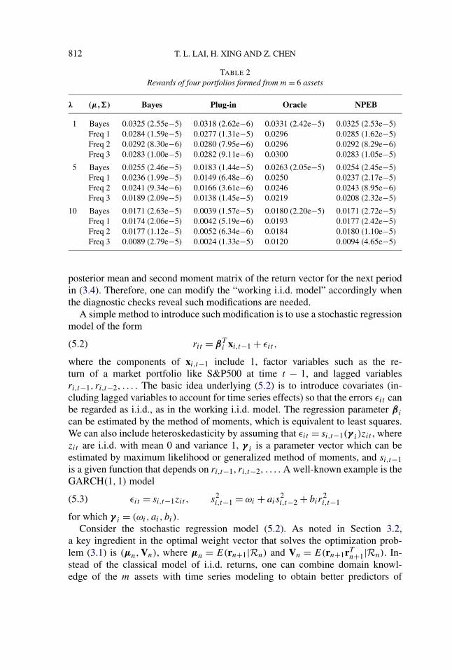
An obvious way of dimension reduction when there is no short selling is toexclude assets with markedly inferior information ratios from consideration. Theonly potential advantage of including them in the portfolio is that they may be ableto reduce the portfolio variance if they are negatively correlated with the “superior”assets. However, since the correlations are unknown, such advantage is unlikelywhen they are not estimated well enough. Suppose we include in the simulationstudy of Section 4.2 two more assets so that all asset returns are jointly normal.The additional hyperparameters of the normal and inverted Wishart prior distribu-tion (2.2) are ν5 = −0.014, ν6 = −0.064, �55 = 2.02, �66 = 10.32, �56 = 0.90,�15 = −0.17, �25 = −0.03, �35 = −0.91, �45 = −0.33, �16 = −3.40, �26 =−3.99, �36 = −0.08 and �46 = −3.58. As in Section 4.2, we consider four sce-narios for the case of n = 8 without short selling, the first of which assumes thisprior distribution and studies the Bayesian reward for λ = 1,5 and 10. Table 2shows the rewards for the four rules in Section 4.2, and each result is based on 500simulations. Note that the value of the reward function does not show significantchange with the inclusion of two additional stocks, which have negative corre-lations with the four stocks in Section 4.2 but have low information ratios. Thisshows that excluding stocks with markedly inferior information ratios when thereis no short selling can reduce m substantially in practice. In Section 6 we describeanother way of choosing stocks from a universe of available stocks to reduce m.

5.3. Extension to time series models of returns. An important assumption inthe modification of Markowitz’s theory in Section 3.2 is that rt are i.i.d. with meanμ and covariance matrix �. Diagnostic checks of the extent to which this assump-tion is violated should be carried out in practice. The stochastic optimization the-ory in Section 3.1 does not actually need this assumption and only requires the


TABLE 2Rewards of four portfolios formed from m = 6 assets

λ (μ,�) Bayes Plug-in Oracle NPEB




posterior mean and second moment matrix of the return vector for the next periodin (3.4). Therefore, one can modify the “working i.i.d. model” accordingly whenthe diagnostic checks reveal such modifications are needed.

A simple method to introduce such modification is to use a stochastic regressionmodel of the form

rit = βTi xi,t−1 + εit ,(5.2)

where the components of xi,t−1 include 1, factor variables such as the re-turn of a market portfolio like S&P500 at time t − 1, and lagged variablesri,t−1, ri,t−2, . . . . The basic idea underlying (5.2) is to introduce covariates (in-cluding lagged variables to account for time series effects) so that the errors εit canbe regarded as i.i.d., as in the working i.i.d. model. The regression parameter β i

can be estimated by the method of moments, which is equivalent to least squares.We can also include heteroskedasticity by assuming that εit = si,t−1(γ i )zit , wherezit are i.i.d. with mean 0 and variance 1, γ i is a parameter vector which can beestimated by maximum likelihood or generalized method of moments, and si,t−1is a given function that depends on ri,t−1, ri,t−2, . . . . A well-known example is theGARCH(1,1) model

εit = si,t−1zit , s2i,t−1 = ωi + ais

2i,t−2 + bir

2i,t−1(5.3)

for which γ i = (ωi, ai, bi).Consider the stochastic regression model (5.2). As noted in Section 3.2,

a key ingredient in the optimal weight vector that solves the optimization prob-lem (3.1) is (μn,Vn), where μn = E(rn+1|Rn) and Vn = E(rn+1rT

n+1|Rn). In-stead of the classical model of i.i.d. returns, one can combine domain knowl-edge of the m assets with time series modeling to obtain better predictors of


future returns via μn and Vn. The regressors xi,t−1 in (5.2) can be chosen tobuild a combined substantive–empirical model for prediction; see Section 7.5of Lai and Xing (2008). Since the model (5.2) is intended to produce i.i.d.εt = (ε1t , . . . , εmt )

T , or i.i.d. zt = (z1t , . . . , zmt )T after adjusting for conditional

heteroskedasticity as in (5.3), we can still use the NPEB approach to determine theoptimal weight vector, bootstrapping from the estimated common distribution ofεt (or zt ). Note that (5.2) and (5.3) models the asset returns separately, instead ofjointly in a multivariate regression or multivariate GARCH model which has toomany parameters to estimate. While the vectors εt (or zt ) are assumed to be i.i.d.,(5.2) [or (5.3)] does not assume their components to be uncorrelated since it treatsthe components separately rather than jointly. The conditional cross-sectional co-variance between the returns of assets i and j given Rn is given by

Cov(ri,n+1, rj,n+1|Rn) = si,n(γ i )sj,n(γ j )Cov(zi,n+1, zj,n+1|Rn)(5.4)

for the model (5.2) and (5.3). Note that (5.3) determines s2i,n recursively from Rn,

and that zn+1 is independent of Rn and, therefore, its covariance matrix can beconsistently estimated from the residuals zt . Under (5.2) and (5.3), the NPEB ap-proach uses the following formulas for μn and Vn in (3.5):

μn = (βT

1 x1,n, . . . , βT

mxm,n)T , Vn = μnμ

Tn + (si,nsj,nσij )1≤i,j≤n,(5.5)

in which βi is the least squares estimate of βi , and sl,n and σij are the usualestimates of sl,n and Cov(zi,1, zj,1) based on Rn. Further discussion of time seriesmodeling for implementing the optimal portfolio in Section 3 will be given inSections 6.2 and 7.

6. An empirical study. In this section we describe an empirical study of theout-of-sample performance of the proposed approach and other methods for mean–variance portfolio optimization when the means and covariances of the underlyingasset returns are unknown. The study uses monthly stock market data from January1985 to December 2009, which are obtained from the Center for Research in Secu-rity Prices (CRSP) database, and evaluates out-of-sample performance of differentportfolios of these stocks for each month after the first ten years (120 months)of this period to accumulate training data. The CRSP database can be accessedthrough the Wharton Research Data Services at the University of Pennsylvania(http://wrds.wharton.upenn.edu). Following Ledoit and Wolf (2004), at the begin-ning of month t , with t varying from January 1995 to December 2009, we selectm = 50 stocks with the largest market values among those that have no missingmonthly prices in the previous 120 months, which are used as the training sample.The portfolios for month t to be considered are formed from these m stocks.

Note that this period contains highly volatile times in the stock market, such asaround “Black Monday” in 1987, the Internet bubble burst and the September 11terrorist attacks in 2001, and the “Great Recession” that began in 2007 with the

http://wrds.wharton.upenn.edu


default and other difficulties of subprime mortgage loans. We use sliding windowsof n = 120 months of training data to construct portfolios of the stocks for thesubsequent month. In contrast to the Black–Litterman approach described in Sec-tion 2.2, the portfolio construction is based solely on these data and uses no otherinformation about the stocks and their associated firms, since the purpose of theempirical study is to illustrate the basic statistical aspects of the proposed methodand to compare it with other statistical methods for implementing Markowitz’smean–variance portfolio optimization theory. Moreover, for a fair comparison, wedo not assume any prior distribution as in the Bayes approach, and only use NPEBin this study.

Performance of a portfolio is measured by the excess returns et over a bench-mark portfolio. As t varies over the monthly test periods from January 1995 toDecember 2009, we can (i) add up the realized excess returns to give the cumula-tive realized excess return

∑tl=1 el up to time t , and (ii) use the average realized

excess return and the standard deviation to evaluate the realized information ratio√12e/se, where e is the sample average of the monthly excess returns and se is

the corresponding sample standard deviation, using√

12 to annualize the ratio asin Ledoit and Wolf (2004). Noting that the realized information ratio is a summarystatistic of the monthly excess returns in the 180 test periods, we find it more in-formative to supplement this commonly used measure of investment performancewith the time series plot of cumulative realized excess returns, from which therealized excess returns et can be retrieved by differencing.

We use two ways to construct the benchmark portfolio. The first follows that ofLedoit and Wolf (2004), who propose to mimic how an active portfolio managerchooses the benchmark to define excess returns. It is described in Section 6.1. Thesecond simply uses the S&P500 Index as the benchmark portfolio and Section 6.3considers this case. Section 6.2 compares the time series of the returns of these twobenchmark portfolios and explains why we choose to use the S&P500 Index as thebenchmark portfolio in conjunction with the time series model (5.2) and (5.3) forthe excess returns in Section 6.3.

6.1. Active portfolios and associated optimization problems. In this sectionthe benchmark portfolio consists of the m = 50 stocks chosen at the beginningof each test period and weights them by their market values. Let wB denote theweight of this value-weighted benchmark and w the weight of a given portfolio.The difference w = w − wB satisfies wT 1 = 0. An active portfolio manager wouldchoose w that solves the following optimization problem instead of (1.1):

wactive = wB + arg minw

wT �w subject to wT μ = μ∗,(6.1)

wT 1 = 0 and w ∈ C,

in which C represents additional constraints for the manager, � is the covariancematrix of stock returns and μ∗ is the target excess return over the value-weighted


benchmark. The portfolio defined by wactive is called an active portfolio. Since μand � are typically unknown, putting a prior distribution on them in (6.1) leads tothe following modification of (3.1):

max{E(wT rn+1) − λVar(wT rn+1)} subject to wT 1 = 0.(6.2)

This optimization problem can be solved by the same method as that introduced inSection 3.

Following Ledoit and Wolf (2004), we choose the constraint set C such that theportfolio is long only and the total position in any stock cannot exceed an upperbound c, that is, C = {w :−wB ≤ w ≤ c1 − wB}, with c = 0.1. We use quadraticprogramming to solve the optimization problem (6.1) in which μ and � are re-placed, for the plug-in active portfolio, by their sample estimates based on thetraining sample in the past 120 months. The covariance-shrinkage active portfoliouses a shrinkage estimator of � instead, shrinking toward a patterned matrix thatassumes all pairwise correlations to be equal [Ledoit and Wolf (2003)]. Similarly,we can extend Section 2.3 to obtain a resampled active portfolio, and also ex-tend the NPEB approach in Section 4 to construct the corresponding NPEB activeportfolio. Table 3 summarizes the realized information ratio

√12e/se for different

values of annualized target excess returns μ∗ and “matching” values of λ whosechoice is described below.

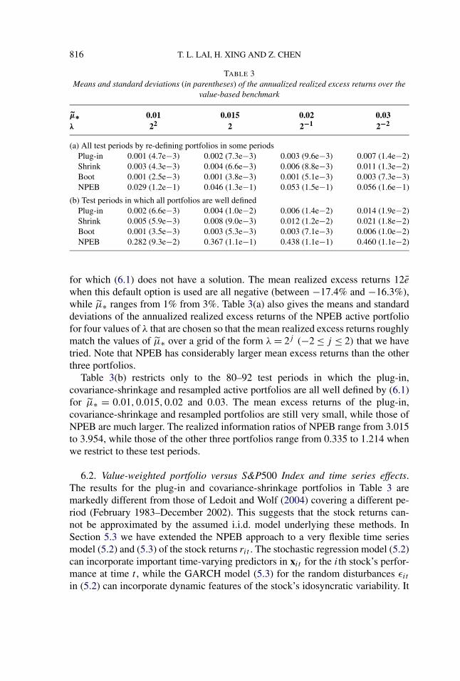
We first note that specified target returns μ∗ may be vacuous for the plug-in, covariance-shrinkage (abbreviated “shrink” in Table 3) and resampled (ab-breviated “boot” for bootstrapping) active portfolios in a given test period. Forμ∗ = 0.01,0.015,0.02,0.03, there are 92, 91, 91 and 80 test periods, respectively,for which (6.1) has solutions when � is replaced by either the sample covariancematrix or the Ledoit–Wolf shrinkage estimator of the training data from the pre-vious 120 months. Higher levels of target returns result in even fewer of the 180test periods for which (6.1) has solutions. On the other hand, values of μ∗ thatare lower than 1% may be of little practical interest to active portfolio managers.When (6.1) does not have a solution to provide a portfolio of a specified type fora test period, we use the value-weighted benchmark as the portfolio for the testperiod. Table 3(a) gives the actual (annualized) mean realized excess returns 12e

to show the extent to which they match the target value μ∗, and also the corre-sponding annualized standard deviations

√12se, over the 180 test periods for the

plug-in, covariance-shrinkage and resampled active portfolios constructed with theabove modification. These numbers are very small, showing that the three portfo-lios differ little from the benchmark portfolio, so the realized information ratiosthat range from 0.24 to 0.83 for these active portfolios can be quite misleading ifthe actual mean excess returns are not taken into consideration.

We have also tried another default option that uses 10 stocks with the largestmean returns (among the 50 selected stocks) over the training period and putsequal weights to these 10 stocks to form a portfolio for the ensuing test period


TABLE 3Means and standard deviations (in parentheses) of the annualized realized excess returns over the

value-based benchmark

μ∗ 0.01 0.015 0.02 0.03λ 22 2 2−1 2−2

(a) All test periods by re-defining portfolios in some periodsPlug-in 0.001 (4.7e−3) 0.002 (7.3e−3) 0.003 (9.6e−3) 0.007 (1.4e−2)Shrink 0.003 (4.3e−3) 0.004 (6.6e−3) 0.006 (8.8e−3) 0.011 (1.3e−2)Boot 0.001 (2.5e−3) 0.001 (3.8e−3) 0.001 (5.1e−3) 0.003 (7.3e−3)NPEB 0.029 (1.2e−1) 0.046 (1.3e−1) 0.053 (1.5e−1) 0.056 (1.6e−1)

(b) Test periods in which all portfolios are well definedPlug-in 0.002 (6.6e−3) 0.004 (1.0e−2) 0.006 (1.4e−2) 0.014 (1.9e−2)Shrink 0.005 (5.9e−3) 0.008 (9.0e−3) 0.012 (1.2e−2) 0.021 (1.8e−2)Boot 0.001 (3.5e−3) 0.003 (5.3e−3) 0.003 (7.1e−3) 0.006 (1.0e−2)NPEB 0.282 (9.3e−2) 0.367 (1.1e−1) 0.438 (1.1e−1) 0.460 (1.1e−2)

for which (6.1) does not have a solution. The mean realized excess returns 12e

when this default option is used are all negative (between −17.4% and −16.3%),while μ∗ ranges from 1% from 3%. Table 3(a) also gives the means and standarddeviations of the annualized realized excess returns of the NPEB active portfoliofor four values of λ that are chosen so that the mean realized excess returns roughlymatch the values of μ∗ over a grid of the form λ = 2j (−2 ≤ j ≤ 2) that we havetried. Note that NPEB has considerably larger mean excess returns than the otherthree portfolios.

Table 3(b) restricts only to the 80–92 test periods in which the plug-in,covariance-shrinkage and resampled active portfolios are all well defined by (6.1)for μ∗ = 0.01,0.015,0.02 and 0.03. The mean excess returns of the plug-in,covariance-shrinkage and resampled portfolios are still very small, while those ofNPEB are much larger. The realized information ratios of NPEB range from 3.015to 3.954, while those of the other three portfolios range from 0.335 to 1.214 whenwe restrict to these test periods.

6.2. Value-weighted portfolio versus S&P500 Index and time series effects.The results for the plug-in and covariance-shrinkage portfolios in Table 3 aremarkedly different from those of Ledoit and Wolf (2004) covering a different pe-riod (February 1983–December 2002). This suggests that the stock returns can-not be approximated by the assumed i.i.d. model underlying these methods. InSection 5.3 we have extended the NPEB approach to a very flexible time seriesmodel (5.2) and (5.3) of the stock returns rit . The stochastic regression model (5.2)can incorporate important time-varying predictors in xit for the ith stock’s perfor-mance at time t , while the GARCH model (5.3) for the random disturbances εit

in (5.2) can incorporate dynamic features of the stock’s idosyncratic variability. It


seems that a regressor such as the return ut of S&P500 Index should be includedin xit to take advantage of the co-movements of rit and ut . However, since ut isnot observed at time t , one may need to have good predictors of ut which shouldconsist not only of the past S&P500 returns but also macroeconomic variables.Of course, stock-specific information such as the firm’s earnings performance andforecast and its sector’s economic outlook should also be considered. This meansthat fundamental analysis, as carried out by professional stock analysts and econo-mists in investment banks, should be incorporated into the model (5.2). Since thisis clearly beyond the scope of the present empirical study whose purpose is toillustrate our new statistical approach to the Markowitz optimization enigma, weshall focus on simple models to demonstrate the benefit of building good modelsfor rt+1 in our stochastic optimization approach.

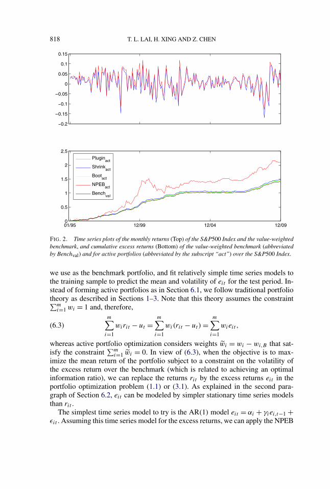
In this connection, we first compare the S&P500 Index with the value-weightedportfolio, which is the benchmark portfolio in Section 6.1. The top panel of Fig-ure 2 gives the time series plots of the monthly returns (which are not annual-ized) of both portfolios during the test period. The S&P500 Index has mean 0.006and standard deviation 0.046 in this period, while the mean of the value-weightedportfolio is 0.0137 and its standard deviation is 0.045. The bottom panel of Fig-ure 2 plots the time series of cumulative realized excess returns

∑tl=1 el over the

S&P500 Index, for the value-weighted portfolio and also for the four active port-folios in Table 3(a) under the column μ∗ = 0.015 and λ = 2, during the test period(January 1995–December 2009). Unlike NPEBact, the cumulative realized excessreturns of the other three active portfolios differ little from the value-weightedportfolio, as shown by the figure.

In view of the structural changes in the economy and the financial marketsduring this period, it appears difficult to find simple time series models that canreflect the inherent nonstationarity. If we use the S&P500 Index ut as an alter-native benchmark to the value-weighted portfolio used in Section 6.1, the excessreturns eit = rit − ut may be able to exploit the co-movements of rit and ut toremove their common nonstationarity due to changes in macroeconomic variables.As an illustration, the top panel of Figure 3 gives the time series plots of returns ofSherwin–Williams Co. (SHW) and of the S&P500 Index during this period, andthe middle panel gives the time series plot of the excess returns. The Ljung–Boxtest, which involves autocorrelations of lags up to 20 months, has p-value 0.001 forthe monthly returns of SHW and 0.267 for the excess returns, and therefore rejectsthe i.i.d. assumption for the actual but not the excess returns; see Section 5.1 of Laiand Xing (2008). This is also shown graphically by the autocorrelation functionsin the bottom panel of Figure 3.

6.3. Using the S&P500 Index as benchmark portfolio and time series models ofexcess returns. The preceding section shows that using the S&P500 Index as thebenchmark portfolio has certain advantages over the value-weighted portfolio. Inthis section we consider the excess returns eit over the S&P500 Index ut , which


FIG. 2. Time series plots of the monthly returns (Top) of the S&P500 Index and the value-weightedbenchmark, and cumulative excess returns (Bottom) of the value-weighted benchmark (abbreviatedby Benchval) and for active portfolios (abbreviated by the subscript “act”) over the S&P500 Index.

we use as the benchmark portfolio, and fit relatively simple time series models tothe training sample to predict the mean and volatility of eit for the test period. In-stead of forming active portfolios as in Section 6.1, we follow traditional portfoliotheory as described in Sections 1–3. Note that this theory assumes the constraint∑m

i=1 wi = 1 and, therefore,m∑

i=1

wirit − ut =m∑

i=1

wi(rit − ut) =m∑

i=1

wieit ,(6.3)

whereas active portfolio optimization considers weights wi = wi − wi,B that sat-isfy the constraint

∑mi=1 wi = 0. In view of (6.3), when the objective is to max-

imize the mean return of the portfolio subject to a constraint on the volatility ofthe excess return over the benchmark (which is related to achieving an optimalinformation ratio), we can replace the returns rit by the excess returns eit in theportfolio optimization problem (1.1) or (3.1). As explained in the second para-graph of Section 6.2, eit can be modeled by simpler stationary time series modelsthan rit .

The simplest time series model to try is the AR(1) model eit = αi + γiei,t−1 +εit . Assuming this time series model for the excess returns, we can apply the NPEB


FIG. 3. Comparison of returns and excess returns. Top panel: returns of S&P500 Index (black) andSHW (red). Middle panel: excess returns (blue) of SHW. Bottom panel: Autocorrelations of returns(red) and excess returns (blue) of SHW; the dotted lines represent rejection boundaries of 5%-leveltests of zero autocorrelation at indicated lag.

procedure in Section 5.3 to the training sample and thereby obtain the NPEBARportfolio for the test sample. The AR(1) model uses xi,t−1 = (1, ei,t−1)

T as thepredictor in a linear regression model for ei,t . To improve prediction performance,one can include additional predictor variables, for example, the return ut−1 of theS&P500 Index in the preceding period. Assuming the stochastic regression modelei,t = (1, ei,t−1, ut−1)βi + εi,t , and the GARCH(1,1) model (5.3) for εi,t , we canapply the NPEB procedure to the training sample and thereby form the NPEBSRGportfolio for the test sample.

Instead of taking long-only positions (i.e., wi ≥ 0 for all i), we also allow shortselling, with the constraint wi ≥ −0.05 for all i, to construct the following port-folios in this section. For the plug-in, covariance-shrinkage and resampled port-folios, which we abbreviate as in Figure 2 but without the subscript “act” (foractive), we use the annualized target return μ∗ = 0.015,0.02,0.03, for which theproblem (1.1) can be solved for all 180 test periods under the weight constraint;note that we use the mean return instead of the mean excess return as the tar-get μ∗. For the NPEBAR and NPEBSRG portfolios, we use the training sampleas in Section 5.1 to choose λ by maximizing the information ratio over the grid


FIG. 4. Realized cumulative excess returns over the S&P500 Index.

λ ∈ {2i : i = −3,−2, . . . ,6}. Figure 4 plots the time series of cumulative realizedexcess returns over the S&P500 Index during the test period of 180 months, forPlug-in, Shrink and Boot with μ∗ = 0.015 and for NPEBAR and NPEBSRG. Ta-ble 4 gives the annualized realized information ratios, with the S&P500 Index asthe benchmark portfolio. The table also considers cases μ∗ = 0.02,0.03, and fur-ther abbreviates Plug-in, Shrink and Boot by P, S, B, respectively.

6.4. Discussion. Our approach may perform much better if the investor cancombine domain knowledge with the statistical modeling that we illustrate here.We have not done this in the present comparative study because using a purely

TABLE 4Realized information ratios and average realized excess returns (in square brackets) with respect to

the S&P500 Index

μ∗ = 0.015 μ∗ = 0.02 μ∗ = 0.03 NPEB

P S B P S B P S B AR SRG

0.527 0.352 0.618 0.532 0.353 0.629 0.538 0.354 0.625 0.370 1.169[0.078] [0.052] [0.077] [0.078] [0.051] [0.078] [0.076] [0.050] [0.077] [0.283] [0.915]


empirical analysis of the past returns of these stocks to build the predictionmodel (5.2) would be a disservice to the power and versatility of the proposed ap-proach, which is developed in Section 3 in a general Bayesian framework, allowingthe skillful investor to make use of prior beliefs on the future return vector rn+1and statistical models for predicting rn+1 from past market data. The prior beliefscan involve both the investor’s and the market’s “views,” as in the Black–Littermanapproach described in Section 2.2, for which the market’s view is implied by theequilibrium portfolio. Note that Black and Litterman model the potential errors ofthese views by normal priors whose covariance matrices reflect the uncertainties.Our Bayesian approach goes one step further to account for these uncertaintiesby using the actual means and variances of the portfolio’s return in the optimiza-tion problem (3.1), instead of the estimated means and variances in the plug-inapproach.

A portfolio on Markowitz’s efficient frontier can be interpreted as a minimum-variance portfolio achieving a target mean return, or a maximum-mean portfolio ata given volatility (i.e., standard derivation of returns). Portfolio managers preferthe former interpretation, as target returns are appealing to investors. In activeportfolio management [Grinold and Kahn (2000)], this has led to the target excessreturn μ∗ and the optimization problem (6.1). The empirical study in Section 6.1shows that when the means and covariances of the stock returns are unknown andare estimated from historical data, putting these estimates in (6.1) may not providea solution; moreover, the actual mean of the solution (when it exists) can differsubstantially from μ∗.

7. Concluding remarks. The “Markowitz enigma” has been attributed to(a) sampling variability of the plug-in weights (hence use of resampling to cor-rect for bias due to nonlinearity of the weights as a function of the mean vectorand covariance matrix of the stocks) or (b) inherent difficulties of estimation ofhigh-dimensional covariance matrices in the plug-in approach. Like the plug-in ap-proach, subsequent refinements that attempt to address (a) or (b) still follow closelyMarkowitz’s solution for efficient portfolios, constraining the unknown mean toequal to some target returns. This tends to result in relatively low information ratioswhen no or limited short selling is allowed, as noted in Sections 4.3 and 6. Anotherdifficulty with the plug-in and shrinkage approaches is that their measure of “risk”does not account for the uncertainties in the parameter estimates. Incorporatingthese uncertainties via a Bayesian approach results in a much harder stochastic op-timization problem than Markowitz’s deterministic optimization problem, whichwe have been able to solve by introducing an additional parameter η.

Our solution of this stochastic optimization problem opens up new possibilitiesin extending Markowitz’s mean–variance portfolio optimization theory to the casewhere the means and covariances of the asset returns for the next investment periodare unknown. As pointed out in Section 5.3, our solution only requires the posteriormean and second moment matrix of the return vector for the next period, and one


can combine the Black–Litterman-type expert views with statistical modeling todevelop Bayesian or empirical Bayes models with good predictive properties, forexample, by using (5.2) with suitably chosen xi,t−1.

Acknowledgment. We thank the referees for their helpful comments and sug-gestions.

SUPPLEMENTARY MATERIAL

Supplement: Matlab implementation of the NPEB method (DOI: 10.1214/10-AOAS422SUPP; .zip). The source code of our approach is provided.

REFERENCES

BEST, M. J. and GRAUER, R. R. (1991). On the sensitivity of mean–variance-efficient portfolios tochanges in asset means: Some analytical and computational results. Rev. Fin. Stud. 4 315–342.

BICKEL, P. J. and LEVINA, E. (2008). Regularized estimation of large covariance matrices. Ann.Statist. 36 199–227. MR2387969

BLACK, F. and LITTERMAN, R. (1990). Asset Allocation: Combining Investor Views with MarketEquilibrium. Goldman, Sachs and Co., New York.

BRITTEN-JONES, M. (1999). The sampling error in estimates of mean–variance efficient portfolioweights. J. Finance 54 655–671.

BROADIE, M. (1993). Computing efficient frontiers using estimated parameters. Ann. Oper. Res. 45(Special Issue on Financial Engineering) 21–58.

CANNER, N., MANKIW, G. and WEIL, D. N. (1997). An asset allocation puzzle. Amer. Econ. Rev.87 181–191.

CHOPRA, V. K., HENSEL, C. R. and TURNER, A. L. (1993). Massaging mean–variance inputs:Returns from alternative global investment strategies in the 1980s. Management Sci. 39 845–855.

FABOZZI, F. J., KOLM, P. N., PACHAMANOVA, P. A. and FOCARDI, S. M. (2007). Robust PortfolioOptimization and Management. Wiley, New York.

FAN, J., FAN, Y. and LV, J. (2008). High dimensional covariance matrix estimation using a factormodel. J. Econometrics 147 186–197. MR2472991

FRANKFURTER, G. M., PHILLIPS, H. E. and SEAGLE, J. P. (1976). Performance of the Sharpeportfolio selection model: A comparison. J. Financ. Quant. Anal. 6 191–204.

GRINOLD, R. C. and KAHN, R. N. (2000). Active Portfolio Management, 2nd ed. McGraw-Hill,New York.

HUANG, J. Z., LIU, N., POURAHMADI, M. and LIU, L. (2006). Covariance matrix selection andestimation via penalized normal likelihood. Biometrika 93 85–98. MR2277742

JOBSON, J. D. and KORKIE, B. (1980). Estimation for Markowitz efficient portfolios. J. Amer.Statist. Assoc. 75 544–554. MR0590686

JORION, P. (1986). Bayes–Stein estimation for portfolio analysis. J. Financ. Quant. Anal. 21 279–292.

LAI, T. L. and XING, H. (2008). Statistical Models and Methods for Financial Markets. Springer,New York. MR2434025

LEDOIT, P. and WOLF, M. (2003). Improved estimation of the covariance matrix of stock returnswith an application to portfolio selection. J. Empirical Finance 10 603–621.

LEDOIT, P. and WOLF, M. (2004). Honey, I shrunk the sample covariance matrix. J. Portfolio Man-agement 30 110–119.

MARKOWITZ, H. M. (1952). Portfolio selection. J. Finance 7 77–91.

http://dx.doi.org/10.1214/10-AOAS422SUPP

http://www.ams.org/mathscinet-getitem?mr=2387969





http://dx.doi.org/10.1214/10-AOAS422SUPP


MARKOWITZ, H. M. (1959). Portfolio Selection. Wiley, New York. MR0103768MEUCCI, A. (2005). Risk and Asset Allocation. Springer, New York. MR2155219MEUCCI, A. (2010). The Black–Litterman approach: Original model and extensions. In The Ency-

clopedia of Quantitative Finance (R. Cont, ed.) 1 196–199. Wiley, New York.MICHAUD, R. O. (1989). Efficient Asset Management. Harvard Business School Press, Boston, MA.PRESS, W. H., TEUKOLSKY, S. A., WETTERLING, W. T. and FLANNERY, B. P. (1992). Numerical

Recipes in C, 2nd ed. Cambridge Univ. Press, Cambridge. MR1201159ROSS, S. A. (1976). The arbitrage theory of capital asset pricing. J. Econ. Theory 13 341–360.

MR0429063SHARPE, W. F. (1964). Capital asset prices: A theory of market equilibrium under conditions of risk.

J. Finance 19 425–442.SIMANN, Y. (1997). Estimation risk in portfolio selection: The mean variance model versus the mean

absolute deviation model. Management Sci. 43 1437–1446.

T. L. LAI

DEPARTMENT OF STATISTICS

STANFORD UNIVERSITY

PALO ALTO, CALIFORNIA 94305USAE-MAIL: [email protected]

T. XING

DEPARTMENT OF APPLIED MATHEMATICS

AND STATISTICS

STATE UNIVERSITY OF NEW YORK

AT STONY BROOK

STONY BROOK, NEW YORK 11794USAE-MAIL: [email protected]

Z. CHEN

BOSERA FUNDS

SHENZHEN

CHINA

E-MAIL: [email protected]





mailto:[email protected]



mean-variance portfolio optimization when means and

Documents