measures of variabilitykme52026/watkins_variability.pdf · ann e. watkins cal state northridge...

Ann E. Watkins Cal State Northridge September 2014 1

Measures of Variability Statistics has been called the study of variability.

According to the California Common Core State Standards, what measures of variability must secondary school students learn?


Interquartile range

6th grade, Algebra I, Mathematics I, Statistics and Probability Mean absolute deviation

6th grade, 7th grade Standard deviation

Algebra I, Mathematics I, Algebra II, Mathematics III, Statistics and Probability, AP Statistics

Variance

AP Statistics


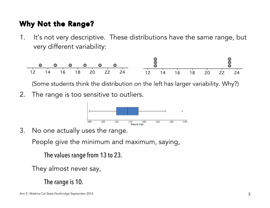
Why Not the Range? 1. It’s not very descriptive. These distributions have the same range, but

very different variability:

(Some students think the distribution on the left has larger variability. Why?)

2. The range is too sensitive to outliers.

3. No one actually uses the range.

People give the minimum and maximum, saying,

The values range from 13 to 23.

They almost never say,

The range is 10.

Top12 14 16 18 20 22 24

Examples Dot Plot

Bottom12 14 16 18 20 22 24

Examples Dot Plot


Interquartile Range

The interquartile range (IQR) is a measure of the variability of the values in a distribution. It is the difference between the third quartile and the first quartile:

IQR = Q3 – Q1

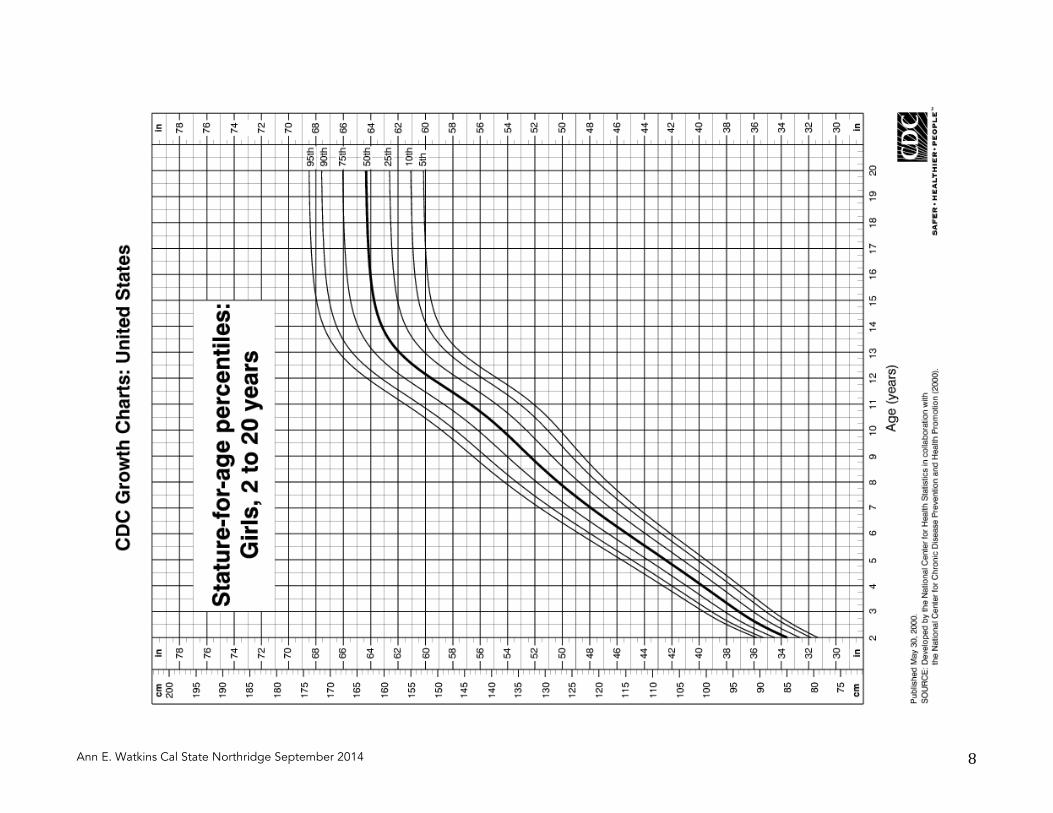
Example The heights of children the same age are quite variable. CDC growth charts contain an amazing amount of information about that variability.

What is the approximate percentile for a 9-year-old girl who is 49 in tall?

About how tall does a 12-year-old girl have to be so that she is as tall or taller than 75% of the girls her age? How tall does a 12-year-old boy have to be?


How can you tell from the chart when children are growing the fastest?

At what age is the rate of increase in height the greatest for girls? For boys?

Is there more variability in the heights of 2-year-old girls or 14-year-old girls?

Is there more variability in the heights of 20-year-old girls or 20-year-old boys?


Estimate the 25th percentile of height for 4-year-old boys. The 50th percentile. The 75th percentile.

Estimate the IQR of heights for 4-year-old boys.

Write a sentence, in context, interpreting the IQR for 4-year-old boys.


The IQR and the Boxplot (Grade 6, Algebra 1, Math I, S&P) Example Two psychologists randomly divided 139 students into three groups. Group 1 learned the names of the others using the “name game,” where the first student states their full name, the second student states their full name and that of the first student and so on. Group 2 learned the names using the name game with the addition that each student stated their favorite activity. In Group 3, each student learned the names by going around and introducing him or herself to each of the other students. One year later the students were sent photos of the others in the group and asked to give the names of as many other students as he or she could remember. The variable recorded for each student was the percentage of names he or she recalled. Here are the results.

Which method would you choose as most effective?

Which group has the most variability in the percentages recalled?

The IQR is equal to the length of the

0 20 40 60 80 100PercentRecalled

Remembering People's Names Box Plot


Example Boxplots are especially useful when you have many groups to compare, each with many cases. For example, the graphs of the ages of females and males with various first names on the next two pages contain 25 boxplots (without whiskers), each of which may summarize the ages of millions of people. fivethirtyeight.com/features/how-to-tell-someones-age-when-all-you-know-is-her-name/ using Social Security Administration records

Why do you think the whiskers weren’t included?

The median for a given name is the age at which half of the females are younger and half are older. Estimate the median age of the Emilys.

The endpoints of the boxes are at the 25th and 75th percentiles. The 25th percentile for a given name is the age at which 25% of the females are younger and 75% are older. Estimate the 25th percentile for the Emilys. Estimate the 75th percentile.

Use the 75th percentile in a sentence about the Donnas.

For which name is the box the longest? What does this tell you about that name?


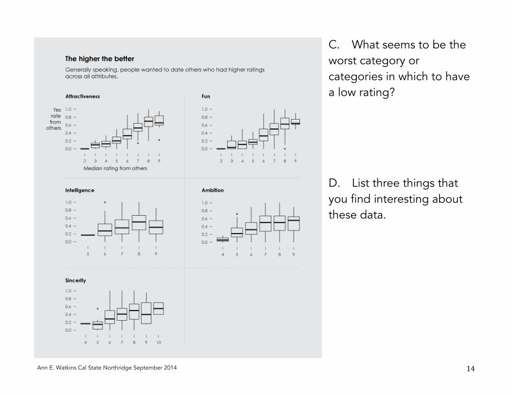
Group Activity The boxplots on the next page show how efficient boxplots can be in displaying a lot of information. The researcher who made them explains, “A few years ago I downloaded speed dating data from experiments conducted by Raymond Fisman, et al. (2005), which represents about 8,000 dates by 551 people. On each date, people scored each other on attractiveness, intelligence, ambition, and some other things, along with a yes or a no to seeing the other person again on a regular date.” theoldreader.com/profile/603ece92bbd932a4a9805cdf For example, the right-most box in the set of boxplots on Attractiveness, represents all of the people who got a median rating of 9 on attractiveness from the other people. The vertical axis gives the proportion of the other people who said “yes” to dating him or her. The outlier is a person who got a median attractiveness rating of 9 from other people, yet only about 0.2, or 20%, said they would like to date him or her. A. In general, were people who were rated higher on these categories more

desirable as a date than those who rated lower?

B. Is there a category that contains an exception to your answer to part A?


C. What seems to be the worst category or categories in which to have a low rating?

D. List three things that you find interesting about these data.


Note: On #6, if a hand span is below the mean, the difference will be negative.


Mean Absolute Deviation (MAD ) One way to think about the variability in data is to examine how far the data values are from their mean.

Group Activity Four Brownie Girl Scout troops each have nine girls. The number of boxes each girl sold on Saturday are given below. (Idea for activity from Jennifer

Kaplan and Robert Floden.)

Troop A: 2, 3, 4, 5, 6, 7, 8, 9, 10 Troop B: 2, 2, 2, 6, 6, 8, 9, 9, 10 Troop C: 2, 6, 6, 6, 6, 6, 6, 6, 10 Troop D: 2, 5, 6, 6, 6, 6, 6, 7, 10

A. Verify that the mean number of boxes sold by the girls in each troop is 6.


B. Which troop is closer to having an equal distribution? Rank the groups from least to most equally distributed. Explain your reasoning with the help of the dot plots and/or with computations.

Number_of_Boxes2 3 4 5 6 7 8 9 10

Boxes of Cookies Sold Dot Plot


C. Several students used the following method to measure how far each Brownie troop was from an equal distribution. Fill in the table for Troop C.

Troop A Troop C Number of Boxes Sold

Distance from Mean of 6

Number of Boxes Sold

Distance from Mean of 6

2 4 3 3 4 2 5 1 6 0 7 1 8 2 9 3

10 4 Total 20

D. Is the distribution of Troop A or Troop C more variable according to the method devised by these students?


E. The students’ method works out well because the troops are all the same size. Now suppose that Troop E has 40 girls, 20 of whom sold 5 boxes and 20 of whom sold 7 boxes. What is the mean for Troop E?

F. Using the students’ method, what is the sum of the distances from the mean for Troop E?

G. Does it seem sensible to say that the sales from Troop E are more variable than from Troop A?


To account for different group sizes, the sum of the distances from the mean is divided by the group size, resulting in the mean absolute deviation.

Mean Absolute Deviation The mean absolute deviation (MAD) is a measure of the variability of n values from their mean:

𝑀𝐴𝐷 = 𝑥 − 𝑥 𝑛

𝑥 − 𝑥 is called a deviation from the mean.

Compute and then compare the MAD for Troop A and Troop E.


Examine the formula for the mean absolute deviation.

Define a deviation from the mean using words only.

Why are the absolute value signs needed? Using Troop A as an example, what would happen if (𝑥 − 𝑥) were computed rather than 𝑥 − 𝑥 ?

What is (𝑥 − 𝑥) always equal to?


The Standard Deviation The standard deviation is a third measure of variability. Like the MAD, the standard deviation is based on the deviations from the mean, but instead of taking the absolute value of each deviation, each deviation is squared.

Standard Deviation The standard deviation (SD or s) is another measure of the variability of n values from their mean

𝑆𝐷 = 𝑥 − 𝑥 !

𝑛 − 1


Example Complete the table to compute the standard deviation of the number of boxes sold for Troop A.

Number of Boxes Sold, x

Deviation from the Mean, 𝑥 − 𝑥

Squared Deviation from the Mean, 𝑥 − 𝑥 !

2 3 4 5 6 7 8 9

10 Total 0 boxes _________ squared boxes

𝑆𝐷 = !!! !

!!!=


Why Divide By n – 1 in the Formula for the Sample Standard Deviation? Suppose you have a population that consists only of the three numbers 2, 4, and 6. You take a sample of size 2, replacing the first number before you select the second. a. Finish the list of all 9 possible samples you could get in the first column of the chart below. (Order matters so 2, 4

is different from 4, 2.) Then complete each column.

Sample Mean Variance,

dividing by n = 2 Variance, dividing

by n - 1 = 1

2, 2 2 0 0 2, 4 3 1 2

Average

b. Compute the average of each column.

c. Compute the variance of the population {2, 4, 6} (dividing by n) and compare to your answers in part (e).

d. On the average, do you get a better estimate of the variance of the population if you divide by n or by n – 1? Explain.

e. If you divide by n, rather than n – 1, does the variance tend to be too big or too small on average?


Comparing the Measures of Variabi l i ty Students must learn three ways to measure the variability of a distribution: the IQR, the MAD, and the standard deviation. Often, but not always, when comparing distributions each of these measures will give the same answer as to which has the most variability and which has the least.

• Generally, the IQR is the most useful when the distribution is strongly skewed or has outliers.

• The standard deviation is the most commonly reported measure of variability. It has important mathematical properties and is most useful with symmetric distributions.

• The MAD is used mainly to introduce the idea of deviation from the mean to middle school students as a prelude to the standard deviation.

What can you conclude if the MAD of a set of data is 0?

What can you conclude if the SD is 0?

What can you conclude if the IQR is 0?


Sample Homework 1. Refer to the growth charts.

a. What is the approximate percentile for an 8-year-old girl who is 50 inches tall?

b. About how tall does a 10-year-old girl have to be so that she is as tall or taller than 75% of the girls her age? How tall does a 10-year-old boy have to be?

c. What is the 25th percentile of height for 6-year-old boys? The 50th percentile? The 75th percentile?

d. Compute and interpret the IQR of heights for 6-year-old boys.

e. Is there more variability in the heights of 6-year-old boys or 12-year-old boys? How can you tell from the charts?

f. Is there more variability in the heights of 5-year-old girls or 5-year-old boys? How can you tell from the charts?


2. Refer to the cookie sales for the four Brownie troops.

a. Compute the mean absolute deviation and the standard deviation for the four troops (some were done in class). Round to the nearest tenth and record your results in the table below.

Troop MAD SD

A

B

C

D

b. Rank the four troops according to their variability from the mean from smallest to largest. Does it matter whether you use the MAD or the SD to do the ranking?


3. You may have learned about the range as a measure of variability:

range = maximum – minimum

a. What is the range of the number of boxes sold by the Brownies in Troop A? Troop B? Troop C? Troop D?

b. Why are the MAD and the SD better measures of variability in a distribution than is the range?

c. Is the range resistant to outliers? Is the interquartile range resistant to outliers?

d. Does the distribution on the left or the right below have the larger variability?

e. Many middle school students pick the wrong distribution in part c. Can you explain what they are thinking?


4. You may have used the distance formula to compute the distance, d, between two points in the plane, (x1, y1) and (x2, y2):

d = 𝑥! − 𝑥! ! + 𝑦! − 𝑦! !

a. Use the distance formula to compute the distance between the points (4, 4) and (6, 2).

b. Compute the standard deviation of the values 6 and 2.

c. Compare the processes you used in parts a and b. What’s the same? What’s different?


5. Does the statement below describe the mean absolute deviation or the standard deviation?

It is the sum of the distances from the mean.

6. The dotplots below give the pesticide concentrations at three depths in a river. Answer the questions without computing.

a. Which depth has the largest mean? The largest standard deviation?

b. Which has the smallest mean? The smallest standard deviation?


7. Match each of the following histograms of test scores in Classes I, II, and III to the best description of class performance.

a. The mean of the test scores is 46, and the standard deviation is 26.

b. The mean of the test scores is 46, and the standard deviation is 8.

c. The mean of the test scores is 46, and the standard deviation is 16.


8. No computing should be necessary to answer these questions.

a. The mean of each of these sets of values is 20, and the range is 40. Which has the largest standard deviation? Which has the smallest?

I. 0 10 20 30 40

II. 0 0 20 40 40

III. 0 19 20 21 40

b. Two of these sets of values have a standard deviation of about 5. Which two?

I. 5 5 5 5 5 5

II. 10 10 10 20 20 20

III. 6 8 10 12 14 16 18 20 22

IV. 5 10 15 20 25 30 35 40 45

c. The standard deviation of the first set of values listed below is about 32. What is the standard deviation of the second set? Explain your answer.

16 23 34 56 78 92 93

20 27 38 60 82 96 97


9. Write the letter of the histogram next to the appropriate set of summary statistics. From Activity-Based Statistics, Scheaffer et al.


http://www.amstat.org/education/usefulsitesforteachers.cfm

measures of variabilitykme52026/watkins_variability.pdf · ann e. watkins cal state northridge...

Documents