mergers - department of economics · vertical mergers are mergers between firms at different...
TRANSCRIPT
MERGERS
1. TYPES OF MERGERS
1.1. Horizontal. Horizontal mergers are mergers between firms which were formerly competitors. A hor-izontal merger involves two firms who produce products that are considered substitutes by their buyers orby two firms who purchase the same or substitute products in the input market.
1.2. Vertical. Vertical mergers are mergers between firms at different stages of the production chain ormore generally between firms that produce complementary goods such as feeder cattle and slaughter cattle,crude oil and gasoline, broiler production and broiler processing, chemical herbicides and particular typesof seed, communications firms operating in different markets, etc.
1.3. Conglomerate. Conglomerate mergers are mergers between firms without a clear substitute or clearcomplementary relationship.
2. HORIZONTAL MERGERS
2.1. A Simple Cournot Model.
2.1.1. Assumptions and structure of the model.
1. N ≥ 2 firms in the industry2. Identical and constant costs for each firm given by C(qj) = cqj , j = 1,2, ... , N3. Linear inverse demand given by
p = A − BQ
= A − B (q1 + · · · + qi−1 + qi + qi+1 + · · ·+ qN )
= A − B (Σj 6=i qj) − B qi
= A − B Q−i − B qi
(1)
4. Industry supply given by Q = Q−i + qi , Q−i = Σj 6=i qj
5. Profit for the ith firm given by
πi = maxqi
[p qi − C(qi)]
= maxqi
[(A − B Q−i − B qi) qi − c qi]
= maxqi
[A qi − B Q−i qi − B q2i − c qi]
(2)
Date: December 16, 2004.1
2 MERGERS
2.1.2. Profit maximization for a representative firm. Optimizing the profit expression with respect to qi willgive
πi = A qi − B Q−i qi − B q2i − c qi
dπi
dqi= A − B Q−i − 2 B qi − c = 0
⇒ 2 B qi = A − B Q−i − c
⇒ q∗i =A − c
2 B− Q−i
2
(3)
Since all firms are identical, this holds for all other firms too.
2.1.3. Nash equilibrium. In a Nash equilibrium, each firm i chooses a best response q∗i that reflects a correct
prediction of the other N-1 outputs in total. Denote this sum as Q∗−i. A Nash equilibrium is then
q∗i =A − c
2 B−
Q∗−i
2(4)
Because all the firms are identical we can write Q∗−i = Σi6=j q∗
j = (N − 1) q∗ where q* is the optimal out-put for the identical firms. We can then write
q∗ =A − c
2 B− (N − 1) q∗
2
⇒ 2 q∗ + (N − 1)q∗
2=
A − c
2 B
⇒ (N + 1)q∗
2=
A − c
2 B
⇒ q∗ =A − c
(N + 1) B
(5)
Industry output and price are given by
Q∗ =N (A − c)(N + 1) B
p∗ = A − BQ∗
= A − B
(N (A − c)(N + 1) B
)
=(N + 1) A
N + 1− N A
(N + 1)− N c
N + 1
=A
N + 1+
N
N + 1c
(6)
The ith firm has profit equal to
MERGERS 3
πi = p∗q∗i − c q∗i
=(
A
N + 1+
N
N + 1c
)q∗i − c q∗i
=(
A
N + 1+
(N
N + 1− 1
)c
)q∗i
=[
A
N + 1+
(N
N + 1− 1
)c
] [A − c
(N + 1) B
]
=[
A
N + 1+
(N − N − 1
N + 1
)c
] [A − c
(N + 1) B
]
=[
A − c
N + 1
] [A − c
(N + 1) B
]
=(A − c) 2
(N + 1) 2 B
(7)
2.1.4. Merger of M ≤ N firms. If M of the N firms in the industry merge then there are N-M+1 independentfirms left in the industry. This merged firm is comprised of firms 1 through M. The merged firm picksoutput QM = q1 + q2 + . . . + qM . The profit maximization problem for the merged firm is given by
πM = maxQM
[p QM − cQM ]
= maxqM
[(A − B Q−M − B QM ) QM − c QM ]
= maxQM
[A QM − B Q−M QM − B Q2M − c QM ]
(8)
The profit maximization problem for each of the remaining independent firms is given by
πi = maxqi
[p qi − cqi]
= maxqi
[(A − B Q−i − B qi) qi − c qi]
= maxqi
[A qi − B Q−i qi − B q2i − c qi]
(9)
Here Q−i denotes the aggregate output of all N-M firms other than the ith firm including the output ofthe merged firm QM. After the merger the merged firm is just like any one of the other m+1, m+2, ... , N in theindustry.
2.1.5. Industry Equilibrium. Because the problem is analogous to the one in equation 2, we can use theresults and intuition from that problem to obtain the equilibrium quantities
4 MERGERS
Q∗M =
(A − c)(N − M + 2) B
q∗i =(A − c)
(N − M + 2) B, i 6∈ M
Q∗ = Q∗M + (N − M ) (q∗i ) = (N − M + 1)
((A − c)
(N − M + 2) B
)
=(
(N − M + 1) (A − c)(N − M + 2) B
)
(10)
The equilibrium price is given by
p∗ = A − BQ∗
= A − B
((N − M + 1) (A − c)
(N − M + 2) B
)
=(N − M + 2) A
N − M + 2− (N − M + 1) A
(N − M + 2)− (N − M + 1) c
N − M + 2
=A
N − M + 2+
N − M + 1N − M + 2
c
(11)
Similarly profits are given by
πM = πi = p∗q∗M − cq∗M
=(
A
N − M + 2+
N − M + 1N − M + 2
c
)Q∗
M − c Q∗M
=[
A
N − M + 2+
(N − M + 1N − M + 2
− 1)
c
] [A − c
(N − M + 2) B
]
=[
A − c
N − M + 2
] [A − c
(N − M + 2) B
]
=(A − c) 2
(N − M + 2) 2 B
(12)
Equations 7 and 12 allow us to compare the profit of the non-merging firms before and after the othersmerge. It is clear that profits are larger after the merger for the firms who do not merge because the denom-inator in equation 12 is smaller than the denominator in equation 7 if M is larger than 1. Now consider thefirms who merged. Prior to the merger they each earned the profit in equation 7. Their total profit is givenby M times this amount or
πM(pre − merger) ≡ M(A − c) 2
(N + 1) 2 B(13)
After the merger they get the amount in equation 12. For profits to be higher it must be that
MERGERS 5
(A − c) 2
(N − M + 2) 2 B≥ M
((A − c)2
B (N + 1)2
)
⇒ (N + 1)2 ≥ M (N − M + 2)2(14)
This condition is very hard to satisfy unless M is very close to N. For example if N = 3 and M = 2, equation13 would imply 16 ≥ 18 which is false. Similarly if N = 10 and M = 7, equation 14 would imply 121 ≥ 175.If N = 10 and M = 9, equation 14 implies 121 ≥ 81. The tendency seems to be for mergers to pay off onlywhen the merged firm is a large portion of the industry. For example if half the firms merge so that 2M = Nequation 14 implies
(2M + 1)2 ≥ (M ) (2M M + 2)2
⇒ 4M2 + 4M + 1 ≥ M3 + 4M2 + 4M
⇒ 1 ≥ M
(15)
It turns out that M must comprise greater than 80 per cent of the market for the merger to lead to higherprofits.
2.1.6. Criticism of this model. The key result of the model is that the merged firm ends up being just anotherplayer in a Cournot game and gains no advantage due to the merger. This is clearest in a triopoly settingwhere two firms merge. The merged firms would then share half of the market.
2.2. A Stackelberg Model of Mergers.
2.2.1. Assumptions.
1. N ≥ 2 firms are in the industry. Two firms merge so that M = 2. Let these be denoted firm 1 andfirm 2. Denote the output of these two firms by QM and the output of the other N-M firms as QI. Iis then equal to N-2 for this case.
2. Identical and constant costs for each firm given by C(qj) = cqj , j = 1,2, ... , N3. Linear inverse demand given by
p = A − BQ
= A − B (q1 + · · · + qi−1 + qi + qi+1 + · · ·+ qN )
= A − B QI − B QM
(16)
where QI is the output of all the independent firms. For one of the independent firms residualinverse demand is given by
p = A − B QI−i − Bqi − BQM , QI−i = Σj 6∈Mj 6=i
qj
= A − B Q−i − Bqi, Q−i = Σj 6=i qj
(17)
4. Industry supply given by Q = QI + QM , QI = Σj 6∈M qj
5. The merged firm acts as a Stackelberg leader. The other firms act as followers.
6 MERGERS
2.2.2. The profit maximization problem for a non-merged follower firm. The follower firms will maximize profitstaking the output of the merged firms as given. Because the merged firm moves first, these firms can takethis quantity as given. This makes the problem a sequential as opposed to a simultaneous move game.Profit for the jth firm is given by
πj = maxqj
[p qj − cqj]
= maxqj
[(A − B qj − B QI−j − BQM ) qj − c qj]
= maxqj
[A qj − B qj QI−j − BQMqj − B q2j − c qj]
(18)
Maximizing profit we obtain
dπj
dqj= A − B QI−j − B QM − 2 B qj − c = 0
⇒ 2 B qj = A − B QI−j − B QM − c
⇒ q∗j =A − c
2 B− QM
2− QI−j
2
(19)
This is the reaction function for firm j. The non-merged firm acts like any other Cournot firm (Stackelbergfollower) but now takes the output of both merged and other non-merged firms into account. Because allthese firms are the same we get their total supply by multiplication
QI−j = (I − 1) qj
⇒ qj =QI−j
(I − 1)(20)
If we solve equations 19 and 20 together we obtain
q∗j =A − c
2 B− QM
2−
(I − 1 ) q∗j2
⇒2 q∗j2
+(I − 1 ) q∗j
2=
A − c
2 B− QM
2
⇒ (I + 1) q∗j =A − c
B− QM
⇒ q∗j =A − c
B (I + 1)−
QM
(I + 1)
(21)
Aggregate output by these firms is given by
QI =I
(I + 1)
(A − c
B− QM
)(22)
2.2.3. The profit maximization problem for the merged firm. The merged firm realizes that once it chooses itsoutput, QM, the other firms will use equation 21 to pick their optimal output qj = Rj(QM). Consider theresidual inverse demand for the merged firms which is given by
p = A − B QI − B QM (23)Now substitute in the optimal response function for the independent firms to obtain
MERGERS 7
p = A − B
(I
(I + 1)
) (A − c
B− QM
)− B QM (24)
Profit for the merged firms is given by
πM = maxQM
[p QM − cQM ]
= maxQM
[ (A − B
(I
(I + 1)
) (A − c
B− QM
)− B QM
)QM − c QM
]
= maxQM
[ ((I + 1) A
I + 1−
(I (A − c)(I + 1)
)+
B I QM
I + 1− B (I + 1) QM
I + 1
)QM − c (I + 1)QM
I + 1
]
= maxQM
[ (A − c − B QM
I + 1
)QM
]
= maxQM
[ (A QM − c QM − B Q2
M
I + 1
) ]
(25)
If we now maximize equation 25 with respect to QM, we obtain
dπM
dqM=
d[ (
A QM− c QM− B Q2M
I+1
) ]
d QM= 0
⇒ A − c − 2BQM = 0
⇒ Q∗M =
A − c
2B
(26)
2.2.4. Equilibrium output for an independent firm. The equilibrium output of an independent firm is thengiven by substituting 26 into 21 as follows
q∗j =A − c
B (I + 1)− QM
(I + 1)
=A − c
B (I + 1)− A − c
2B (I + 1)
=A − c
2B (I + 1)
=A − c
2B (N − 1), if M = 2
(27)
Total output of the independent firms is given by
Q∗i =
I (A − c)(I + 1) 2B
=( N − 2) (A − c)
(N − 1) 2B, if M = 2
(28)
8 MERGERS
2.2.5. Equilibrium for the industry. Total industry output is given by adding equations 26 and 28 together toobtain
Q∗ = Q∗i + Q∗
M
=I (A − c)(I + 1) 2B
+A − c
2B
=(2I + 1) (A − c)
(I + 1) 2B
(29)
The industry equilibrium price is given by
p = A − B Q∗
= A − B
[(2I + 1) (A − c)
(I + 1) 2B
]
=2 (I + 1) A
2 (I + 1)−
[(2I + 1) (A − c)
(I + 1) 2
]
= A − B
[(2I + 1) (A − c)
(I + 1) 2B
]
=A + c (2I + 1)
2 (I + 1)
(30)
The merged firm has profit
πM = pQM − c QM
=(
A + c (2I + 1)2 (I + 1)
) [A − c
2B
]− c
[A − c
2B
]
=(
A + 2I c + c − 2c(I + 1)2 (I + 1)
) [A − c
2B
]
=(
A − c
2 (I + 1)
) [A − c
2B
]
=(
(A − c)2
4 B(I + 1)
)
(31)
Each of the independent firms has profit equal to

MERGERS 9
πj = pqj − c qj
=(
A + c (2I + 1)2 (I + 1)
) (A − c
2B (I + 1)
)− c
[A − c
2B (I + 1)
]
=(
A − c
2B (I + 1)
) (A + c (2I + 1)
2 (I + 1)− 2 c (I + 1)
2 (I + 1)
)
=(
A − c
2B (I + 1)
) (A + 2c I + c − 2cI − 2c)
2 (I + 1)
)
=(
A − c
2 (I + 1)
) [A − c
2B (I + 1)
]
=(
(A − c)2
4 B(I + 1)2
)
(32)
The merged firm has profits that are much larger than any individual independent firm. We can alsocompare the profit of this merged firm to the combined profits of the M firms when they were membersof the Cournot equilibrium before the merger. This profit is given by equation 7. We repeat it here forconvenience
πk = p∗q∗k − c q∗k
=(A − c) 2
(N + 1) 2 B
(7′)
For the combined profit after merger to be larger than combined profit before merger it must be true that
((A − c)2
4 B(I + 1)
)≥ M (A − c) 2
(N + 1) 2 B
⇒(
14 (N − M + 1)
)≥ M
(N + 1) 2
⇒ (N + 1) 2 ≥ 4M ((N − M + 1 )
(33)
This equation is satisfied exactly if N = 3 and M = 2. It is true for any N greater than 3 if M = 2.
Now consider the profits of an independent firm. They earn the same amount as the non-merged firmbefore the merger. For them to earn less after the merger it must be true that
((A − c)2
4 B(I + 1)2
)≤ (A − c) 2
(N + 1) 2 B
⇒(
14 (N − M + 1)2
)≤ 1
(N + 1) 2
⇒ (N + 1) 2 ≤ 4 (N − M + 1)2
(34)
As long as N ≥ 4 this will hold true, and non-merging firms will be worse off unless M is also very large.
10 MERGERS
2.2.6. Prices and welfare. It is useful to compare the price cost margin in the Stackelberg merger case withthat prevailing in the initial Cournot equilibrium. The margin in the initial case is computed using equation6. The margin in the Stackelberg case is computed using equation 30. The margins are as follows
pcm(Cournot) =A
N + 1+
N
N + 1c −
(N + 1)c(N + 1)
pcm(Stackelberg) =A + c (2I + 1)
2 (I + 1)− 2(I + 1)c
2(I + 1)
(35)
We can rewrite I in terms of M and N (I = M - N) and then note that prices will be lower with theStackelberg merger if
pcm(Stackelberg) =A + c (2(N − M) + 1)
2 ((N − M) + 1)− 2((N − M) + 1)c
2(N − M + 1)≤ A
N + 1+
N
N + 1c − (N + 1)c
(N + 1)= pcm(Cournot)
A + 2cN − 2cM + c − 2Nc + 2Mc − 2c
2 ((N − M) + 1)≤ A + Nc − Nc − c
N + 1
A − c
2 ((N − M) + 1)≤ A − c
N + 1
N + 1 ≤ 2 (N − M + 1)
⇒ 2M − 1 ≤ N
(36)With M = 2, this implies that for N ≥ 3, the price cost margin is lower with the Stackelberg merger. Thus
consumers seem to be better off. If this is really the case, there would seem to be no reason for anti-trustauthorities to ever oppose mergers.
2.3. Multiple mergers - several leaders and followers.
2.3.1. Assumptions.
1. N firms in the industry2. L leader firms - each formed from a merger of two previously independent firms. These are num-
bered 1, 2, ..., L3. F = N-L follower firms. These are numbered L+1, L+2, ..., N4. Followers take total output of leader firms as given and then individually maximize profit.5. Leader firms engage in Cournot competition vis-a vis each other taking into account the actions of
the follower firms.
MERGERS 11
6. Notation for quantities (number of firms in brackets)
Q = total market quantity supplied and demanded [N ]
qf = output of one independent firm (follower) [1]
q` = output of one of the merged firms (leader) [1]
QL = ΣL`=1 q` = aggregate output of leader firms [L]
QF = ΣFf=1 qf = aggregate output of follower firms [F ]
QL−` = Σ k 6=`kε[1,L]
qk = aggregate output of leader firms except ` [L − 1 = N − F − 1]
QF−f = Σ j 6=fjε[L+1,N ]
qj = aggregate output of follower firms except f [F − 1 = N − L − 1]
(37)
7. Cost of production of quantity qk = cqk.8. Inverse demand is given by
p = A − BQ
= A − BQL − BQF
= A − BQL − BQF−f − Bqf
= A − BQL−` − Bq` − BQF
= A − BQL−` − Bq` − BQF−f − Bqf
(38)
2.4. Profit maximization for a representative follower firm. The profit maximization problem for a typicalfollower firm (taking QL and QF−f as given) is
πFf = max
qf
[p qf − C(qf )]
= maxqf
[(A − B (qf + QF−f + QL) qf − c qf ]
= maxqf
[A qf − Bq2f − BQF−f qf − BQL qf − c qf ]
(39)
Carrying out the maximization will give
dπFf
dqf=
d [A qf − Bq2f − BQF−f qf − B QL qf − c qf ]
dqf= 0
⇒ A− 2B qf − BQF−f − B QL − c = 0
⇒ qf =A − c
2B− QL
2− QF−f
2
(40)
2.4.1. Equilibrium response for the follower firms. The follower firms are all symmetric and so each one willhave the same response function as in equation 40. There are (N-L-1) firms in the group QF−f . Total supplyby these firms is then given by
QF−f = [N − L − 1] qf (41)If we substitute equation 41 into equation 40 we obtain
12 MERGERS
q∗f =A − c
2B− QL
2− QF−f
2
=A − c
2B− QL
2− (N − L − 1) qf
2
⇒ 2qf + Nqf − L qf − qf
2=
A − c
2B− QL
2
⇒ (N − L + 1)2
qf =A − c
2B− QL
2
⇒ q∗f =(A − c)
B (N − L + 1)− QL
(N − L + 1)
(42)
Total supply for the F follower firms is then given by [N-L]q∗f . This gives
QF =(N − L) (A − c)B (N − L + 1)
− (N − L) QL
(N − L + 1)(43)
2.4.2. Profit maximization for a representative leader firm. The profit maximization problem for a typical leaderfirm (taking QL−` and QF as given) is
πL` = max
q`
[p q` − C(q`)]
= maxq`
[(A − B (q` + QF + QL−`) q` − c q`]
= maxq`
[A q` − Bq2` − BQF q` − B QL−` q` − c q`]
(44)
If we now substitute from 43 into 44 we obtain

MERGERS 13
πL` = max
q`
[A q` − Bq2` − BQF q` − B QL−` q` − c q`]
= maxq`
[A q` − Bq2
` − B
[(N − L) (A − c)B (N − L + 1)
− (N − L) QL
(N − L + 1)
]q` − B QL−` q` − c q`
]
= maxq`
(q`
[A − c − Bq` −
B (N − L)B (N − L + 1)
(A − c) + B(N − L) QL
(N − L + 1)− B QL−`
])
= maxq`
(q`
[A − c − BQL − B (N − L)
B (N − L + 1)(A − c) + B
(N − L) QL
(N − L + 1)
])
= maxq`
(q`
[(N − L + 1) (A − c)
(N − L + 1)− B (N − L + 1) QL
(N − L + 1)− (N − L)
(N − L + 1)(A − c) + B
(N − L) QL
(N − L + 1)
])
= maxq`
(q`
[(N − L + 1) (A − c) − B (N − L + 1) QL − (N − L) (A − c) + B (N − L) QL
(N − L + 1)
] )
= maxq`
(q`
[(A − c) − B QL
(N − L + 1)
] )
= maxq`
(q`
[(A − c − B QL−` − B q`
(N − L + 1)
] )
= maxq`
((Aq` − cq` − B QL−`q` − B q2
`
(N − L + 1)
)
(45)Carrying out the maximization will give
dπL`
q`=
d(
(Aq` − cq` −B QL−`q` −B q2`
(N −L + 1)
)
dq`= 0
⇒ A− c − BQL−` − 2 B q` = 0
⇒ q` =A − c
2B− QL−`
2
(46)
2.4.3. Equilibrium response for the leader firms. The leader firms are all symmetric and so each one will havethe same response function as in equation 46. There are (L-1) firms in the group Ql−`. Total supply by thesefirms in then given by
QL−` = [L − 1] q` (47)
If we substitute equation 47 into equation 46 we obtain
14 MERGERS
q∗` =A − c
2B−
QL−`
2
=A − c
2B− ( L − 1) q`
2
⇒ 2q` + ( L − 1) q`
2=
A − c
2B
⇒ ( L + 1) q`
2=
A − c
2B
⇒ q∗` =(A − c)
B (L + 1)
(48)
Total supply for the L leader firms is then given Lq∗` . This gives
QL =L (A − c)B (L + 1)
(49)
We can now find qf and QF by substituting equation 49 into equations 42 and 43.
q∗f =(A − c)
B (N − L + 1)− QL
(N − L + 1)
=(A − c)
B (N − L + 1)− L (A − c)
B (L + 1) (N − L + 1)
=(L + 1) (A − c)
B (L + 1) (N − L + 1)− L (A − c)
B (L + 1) (N − L + 1)
=(A − c)
B (L + 1) (N − L + 1)
(50)
Total supply by the follower firms is
Q∗F =
(N − L) (A − c)B (L + 1) (N − L + 1)
(51)
2.4.4. Industry output. Total industry output is given by adding QL and QF to obtain
Q∗ = Q∗F + Q∗
L
=(N − L) (A − c)
B (L + 1) (N − L + 1)+
L (A − c)B (L + 1)
=(N − L) (A − c)
B (L + 1) (N − L + 1)+
L (N − L + 1) (A − c)B (L + 1) (N − L + 1)
=(N − L + LN − L2 + L) (A − c)
B (L + 1) (N − L + 1)
=(N + LN − L2) (A − c)B (L + 1) (N − L + 1)
(52)
We now have the equilibrium quantities of each leader firm, each follower firm, the aggregate for theleaders and the followers, and the total quantity.
MERGERS 15
2.4.5. Price and price cost margin. The market equilibrium price is given by
p∗ = A − BQ∗
= A − B
[(N + LN − L2) (A − c)B (L + 1) (N − L + 1)
]
=(L + 1) (N − L + 1) A
(L + 1) (N − L + 1)− (N + LN − L2) (A − c)
(L + 1) (N − L + 1)
=A (LN − L2 + L + N − L + 1 − N − LN + L2) + c (N + LN − L2)
(L + 1) (N − L + 1)
=A + c (N + LN − L2)(L + 1) (N − L + 1)
(53)
The price cost margin is given by
p∗ − c =A + c (N + LN − L2)(L + 1) (N − L + 1)
− (L + 1) (N − L + 1) c
(L + 1) (N − L + 1)
=A + c N + cLN − cL2 − cLN + cL2 − cN − c)
(L + 1) (N − L + 1)
=A − c
(L + 1) (N − L + 1)
(54)
2.5. Analysis of equilibrium in horizontal merger models.
2.5.1. Individual firms in the multiple firm merger model with Stackelberg behavior. It is clear by comparing equa-tions 48 and 50 that the leader firms produce more than the follower firms.
2.5.2. Comparison of Stackelberg merger equilibrium with several leaders with regular Cournot equilibrium. TheCournot equilibrium from equation 6 and the Stackelberg one from equation 52 are
Q∗C =
N (A − c)(N + 1) B
Q∗SM =
(N + LN − L2) (A − c)B (L + 1) (N − L + 1)
(55)
If L = 0, they are the same. If L = 1, we have
Q∗C =
N (A − c)(N + 1) B
Q∗SM =
(N + N − 1) (A − c)B (1 + 1) (N − 1 + 1)
=(2N − 1) (A − c)
2BN
(56)
To show that QSM ≥ Qc we must show that
16 MERGERS
(2N − 1) (N + 1) ≥ 2 N2
⇒ (2N2 + N − 1) ≥ 2 N2
⇒ N − 1 ≥ 0
This is always true if N ≥ 1. So the expression is true for L = 1. In general the merger solution will havea larger output if
(N + NL − L2) (A − c)B (L + 1) (N − L + 1)
≥ N (A − c)(N + 1) B
⇒ (N + NL − L2)(L + 1) (N − L + 1)
≥ N
(N + 1)⇒ N2 + N2L − NL2 + N + NL − L2 ≥ N2L − NL2 + NL + N2 − NL + N
⇒ −L2 ≥ − NL
⇒ L2 ≤ NL
⇒ L ≤ N
(57)
This will always be the case. Thus the quantity will always be higher with the mergers.
2.5.3. Comparison of profits for leader and follower firms. Profits for a follower firm are obtained by multiplyingthe price-cost margin by output. This will yield
πFf = qf (p∗ − c)
=(
(A − c)B (L + 1) (N − L + 1)
) (A − c
(L + 1) (N − L + 1)
)
=(
(A − c)2
B (L + 1)2 (N − L + 1)2
)(58)
Profits for a leader firm are obtained by multiplying the price-cost margin by output. This will yield
πL` = q` (p∗ − c)
=(
(A − c)B (L + 1)
) (A − c
(L + 1) (N − L + 1)
)
=(
(A − c)2
B (L + 1)2 (N − L + 1)
)(59)
It is very clear comparing equations 58 and 59 that leaders are more profitable than followers. Thus twofirms who are followers may want to consider merging. But if they merge the number of leaders will rise,the number of followers will fall and the industry price cost margin will change. What we need to discoveris the profit of the currently independent firms in the new equilibrium after merger.
2.5.4. Analysis of incentives to merge. In the new equilibrium N will be one less, and L will be one more.Now consider equation 59 with N-1 replacing N and L+1 replacing L. This will give
πL` (N − 1, L + 1) =
((A − c)2
B (L + 2)2 ((N − 1) − (L + 1) + 1)
)
=(
(A − c)2
B (L + 2)2 (N − L − 1)
) (60)
MERGERS 17
We then compare this to 2 times equation 58. If it is larger then there is an incentive to merge. Writingout the inequality gives
((A − c)2
B (L + 2)2 (N − L − 1)
)≥ 2
((A − c)2
B (L + 1)2 (N − L + 1)2
)(61)
We can then simplify to obtain
2 (L + 2)2 (N − L − 1) ≤ (L + 1)2 (N − L + 1)2
⇒ (2L2 + 8L + 8) (N − L − 1) ≤ (L2 + 2L + 1) (N2 − 2NL + L2 + 2(N − L) + 1)
⇒ 2L2N − 2L3 + 8LN − 10L2 + 8N − 16L − 8 ≤ (L2 + 2L + 1) ((N2 − 2NL + 2N + L2 − 2L + 1)
⇒ 2L2N − 2L3 − 10L2 + 8LN − 16L + 8N − 8 ≤L2 N2 − 2NL3 + 2NL2 + L4 − 2L3 + L2
+ 2L N2 − 4NL2 + 4NL + 2 L3 − 4L2 + 2L
+ N2 − 2NL + 2N + L2 − 2L + 1
⇒ 2L2N − 2L3 − 10L2 + 8LN − 16L + 8N − 8 ≤L2 N2 − 2NL3 + L4 − 2NL2 − 2L2 + 2L N2 + 2NL + N2 + 2N + 1
(62)This expression does not seem to simplify but numerical simulation shows that it is always true so that
there is always an incentive to merge. Thus once mergers begin, they will tend to continue.
2.5.5. Social costs of mergers. Another question is whether the mergers are in the best interest of society. Wecan see from equation 54 that the price-cost margin depends on the number of firms and the number offirms in the leadership position (L). The price cost margin will fall as the industry output rises. Considernow the total industry output in the Stackelberg merger case when two more firms merge. We can considertotal output in equation 52 with the output when N decreases by one and L increases by one. We proceedas follows by rewriting equation 52 and then the inequality
Q∗(N − 1, L + 1) =((N − 1) + (L + 1) (N − 1) − (L + 1)2) (A − c)
B (L + 2) ((N − 1) − (L + 1) + 1)≥ (N + LN − L2) (A − c)
B (L + 1) (N − L + 1)= Q∗(N, L)
⇒ ((N − 1) + (L + 1) (N − 1) − (L + 1)2)
(L + 2) ((N − L − 1)≥ N + LN − L2
(L + 1) (N − L + 1)
⇒ (L + 1) (N − L + 1) ((N − 1) + (L + 1) (N − 1) − (L + 1)2)
(L + 1) (N − L + 1) (L + 2) ((N − L − 1)≥ (L + 2) ((N − L − 1) (N + LN − L2 )
(L + 2) ((N − L − 1) (L + 1) (N − L + 1)(63)
The denominator of equation 63 will always be positive because N > L. Thus we need to show that thenumerator on the left is larger than the numerator on the right. We will first simplify the left hand side andthen the right hand side. Then we will put the information together. First for the left hand side
(L + 1) (N − L + 1)((N − 1) + (L + 1) (N − 1) − (L + 1)2
)= (LN − L2 + N + 1)
(2N + LN − L2 − 3L − 3
)
= (2LN2 + L2N2 − L3N − 3L2N − 3LN )
+ (−2L2N − L3N + L4 + 3L3 + 3L2 )
+ ( 2N2 + LN2 − L2N − 3LN − 3N )
+ ( 2N + LN − L2 − 3L − 3 )
= L4 + 3L3 + 2L2 − 3L − 2L3N − 6L2N + L2N2
− 5LN + 3LN2 + 2N2 − N − 3
(64)Now for the right hand side

18 MERGERS
(L + 2) (N − L − 1) (N + LN − L2 ) = (N + LN − L2 ) (LN − L2 − 3L + 2N − 2)
= (LN2 − L2N − 3LN + 2N2 − 2N )
+ (L2N2 − L3N − 3L2N + 2LN2 − 2LN )
+ (−L3N + L4 + 3L3 − 2L2N + 2L2)
= L4 + 3L3 + 2L2 − 2L3N − 6L2N
+ L2N2 + 3LN2 − 5LN + 2N2 − 2N
(65)
Now take the right hand side of equations 64 and 65 and substitute them in to rewrite the numerators ofequation 63 as follows
L4 + 3L3 + 2L2 − 3L − 2L3N − 6L2N + L2N2 − 5LN + 3LN2 + 2N2 − N − 3 ≥
L4 + 3L3 + 2L2 − 2L3N − 6L2N + L2N2 − 5LN + 3LN2 + 2N2 − 2N(66)
Canceling like terms we obtain
−3L − N − 3 ≥ − 2N
⇒ N ≥ 3L + 3(67)
or alternatively
3L ≤ N − 3
⇒ L ≤ N
3− 1
(68)
Thus output will be higher and prices lower as long as the number of firms in the leader group is lessthan 1/3 of the total firms in the industry. When L+1 is larger than N/3, prices will not fall and quantitysupplied will be lower.
MERGERS 19
3. VERTICAL MERGERS
3.1. Introduction to vertical mergers.
3.1.1. Complementary products. Two inputs (xi, xj) are said to be complementary in production if
∂f (x)∂xi ∂xj
> 0 (69)
The idea is that using them together will increase the productivity of the process. Inputs are said to betechnically competitive if
∂f (x)∂xi ∂xj
< 0 (70)
These definitions hold all other inputs constant. More general definitions are based on the elasticity ofsubstitution or on factor demands. For example we say that two inputs are complements if
σij < 0 (71)
where σij is the elasticity of substitution (Allen, Hicks, or Morishima) between xi and xj . We also say thattwo inputs are gross complements if
∂xi (p, w)∂wj
=∂xi (w, y∗)
∂wj+
∂xi (w, y∗)∂y
∂y (p, w)∂wj
≤ 0 (72)
where xi represents an ordinary demand curve. The idea is that there are economies to using the twoinputs together.
3.1.2. Problem of firms in a vertical chain. Often firms in a vertical chain produce products that are comple-mentary in the sense that the output of one firm is an input for another firm. In such cases the output ofone firm will depend on the output of the other firm.
3.1.3. Problem of two firms producing complementary products. Sometimes consumers may prefer to buy prod-ucts in fixed proportions. Examples include right and left handed gloves, right and left ski boots, oxygenand acetylene, computer chip pairs, etc. In such a situation the demand for one product is clearly related tothe demand for the other product.
3.2. A simple monopoly problem. Assume that there are two goods which are used together in consump-tion. A classic example is nuts and bolts. Assume that each is produced by a monopolist. The nut monopo-list has constant cost equal to cN while the bolt monopolist has constant cost equal to cB. A consumer whowants to buy 100 bolts also wants to buy 100 nuts so it is the combined price pB + pN that is relevant. Letthe demand curve for nut and bolt pairs be given by
Q = A − (pB + pN ) (73)
This is also the demand curve for the individual producers Because the two goods are always bought inpairs. Thus we obtain
QB = A − (pB + pN )
QN = A − (pB + pN )(74)
It is obvious that the price chosen by the other firm affects the demand for a given firm’s product. Nowwrite these demand curves in inverse form as
20 MERGERS
pB = A − pN − QB
pN = A − pB − QN
(75)
We can then write total revenue and marginal revenue as
RB = (A − pN − QB) QB
MRB = A − pN − 2QB
RN = (A − pB − QN ) QN
MRN = A − pB − 2QN
(76)
If we now set these equal to marginal cost we obtain
MRB = A − pN − 2QB = cB
⇒ QB =A − pN − cB
2MRN = A − pB − 2QN = cN
⇒ QN =A − pN − cN
2
(77)
If we now substitute these quantities into the inverse demand curves we obtain
pB = A − pN − QB
= A − pN −(
A − pN − cB
2
)
=(
A − pN + cB
2
)
pN = A − pB − QN
= A − pB −(
A − pB − cN
2
)
=(
A − pB + cN
2
)
(78)
The optimal price for each firm depends on the price charged by the other firm. Whatever price is beingcharged by the bolt maker will be obvious to the nut maker and vice versa. If the bolt maker lowers price,the nut maker will see an increase in demand and so forth. This market will be in equilibrium only whenthe two equations are simultaneously satisfied. We can find this point by substitution as follows
MERGERS 21
pB =(
A − pN + cB
2
)
pN =(
A − pB + cN
2
)
⇒ pB =
A −(
A − pB + cN
2
)+ cB
2
=A
4+
pB
4−
cN
4+
cB
2
⇒ 34
pB =A − cN + 2cB
4
⇒ pB =A − cN + 2cB
3
(79)
Similarly for pN
pN =A − cB + 2cN
3(80)
The total price pN + pB is given by the sum as is equal to
pN + pB =A − cB + 2cN
3+
A − cN + 2cB
3
=2A + cB + cN
3
(81)
The number of pairs sold is
Q = A − (pB + pN )
= A − 2A + cB + cN
3
=A − cB − cN
3
(82)
Now compare this to the result if the two firms were merged and simply chose the total production ofnuts and bolts. Inverse demand is given by
pB + pN = A − Q (83)Revenue and marginal revenue are given by
Revenue = (A − Q) Q
MR = A − 2Q(84)
The marginal cost of production is cB + cN. Equating marginal revenue and marginal costs will give
MR = A − 2Q = cB + cN
⇒ Q =A − cb − cn
2
(85)
22 MERGERS
This is clearly larger than in the case where the monopolists acted independently. Profits are lowerwith separate firms and prices to consumers are higher. The intuition behind the foregoing argument isstraightforward. Each firm’s pricing decision imposes an externality on the other firm. For example, ahigh price for computer hardware will reduce demand for PC’s. It will also reduce demand for programsand operating systems. The first effect is taken into account by the hardware manufacturer. The secondis not. The same is true, of course, in reverse. The software manufacturer does not take into account theimpact its price choice has on the demand for hardware. In the noncooperative equilibrium, the price ofboth goods will be too high. If say, the hardware firm were to cuts its price, this would generate additionaldemand and additional profit for the software firm. However, because the hardware firm does not receiveany of this additional profit, it does not reduce its price. This implies that, with cooperation, both firmswould lower their price and be better off. Consumers, too, would gain as a result of lower prices andexpanded output. One way to achieve the profit and efficiency gains of cooperation is for the two firms tomerge. Such a merger creates a singly entry and, therefore, permits the externality to be internalized. Thecombined hardware and software firm will certainly wish to maximize its total profit which means that itwill wish to price the two individual goods so as to maximize the joint profit of each. Thus, whenever firmswith monopoly power produce complementary products, they have a strong incentive either to merge orto devise some other method to assure cooperative production and pricing of the complementary products.
3.3. Vertical Mergers as a Way to Resolve a Common Type of Complementarity.
3.3.1. The incentive behind vertical mergers. Vertical mergers involve combination of firms at different stagesof the production stream. The convention is to label those firms farthest from the final consumer of theproduct as upstream and those closest to that consumer as downstream. Film companies and movie theatersare an example. In this case, the film company is the upstream firm and the theater that rents the filmand then uses it as an input to provide its customers with a cinematic experience is the downstream firm.Manufacturers and retailers have a similar upstream-downstream relation. The point to understand is thatall such relationships can be usefully viewed through the lens of complementarity. The implication is thatvertical relationships between two firms—each with monopoly power—will lead to suboptimal pricing andeconomic inefficiency in the absence of some mechanism to coordinate the decisions of the two firms. Inthe case of vertically-related firms, this issue is typically referred to as the problem of double marginalization.
3.3.2. Set-up of vertical merger problem.
1. FirmsThere are two firms: a single upstream supplier, the manufacturer, who sells a unique product
to a single downstream firm, the retailer.2. Prices and costs
The manufacturer produces the good at constant unit cost c, and sells it to the retailer at a whole-sale price r. The retailer resells the product to consumers at price p. The retailer has no retailingcost.
3. Demand Consumer demand for the good is described by a linear demand function,
p = A − BQ, with c < A. (86)
4. ProfitBecause the retailer buys a unit of the good at whole price r and simply resells it at price p, the
retailer’s profit can be written as:
ΠD(p, r) = (p − r)Q = (A − BQ) Q − rQ (87)
MERGERS 23
3.3.3. Profit maximization for retailer. Profit will be maximized by choosing an output at which the retailer’smarginal revenue is equal to its cost. Carrying out the optimization will give
d ΠD(p, r)dQ
=d [ (A − BQ) Q − rQ ]
dQ= 0
⇒ A − 2BQ − r = 0
⇒ Q =A − r
2B
(88)
If we substitute this into the demand equation we find the equilibrium price of
p = A − BQ
= A − B
[A − r
2B
]
=[
A + r
2
](89)
Profit is given by
ΠD(p, r) = (p − r)Q =(
A + r
2− r
)Q
=(
A − r
2
) [A − r
2B
]
=(A − r)2
4B
(90)
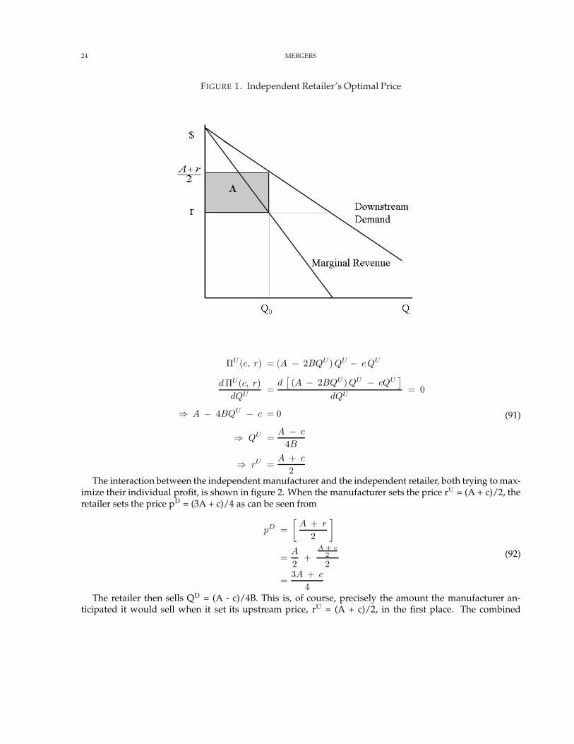
We can represent this graphically as in figure 1The shaded area is the profit for this retailer. The marginal revenue curve is also the demand curve for
the product of the manufacturer. For different values of r, different amounts of the input are demanded.This can be made more formal by noting that quantity sold in the final products market is also the quantitythat must be supplied by the manufacturer. Specifically the quantity Q = (A − r)
2B is the amount of theproduct that the manufacturer will sell to the retailer at price r. We can also solve this equation for theinverse demand curve as
r = A − 2 BQU
where QU denotes the quantity supplied by the wholesaler. In short, the inverse demand facing the upstreammanufacturer at wholesale price r, namely, r = A - 2BQU, is also the marginal revenue function facing the retailer.
3.3.4. Profit maximization for the wholesaler. Because the marginal revenue curve of the retailer and the in-verse demand function confronting the upstream firm are the same, we can formally write the latter as: r= A - 2B QU. This allows us to derive the profit-maximizing price that the upstream firm will set for itsproduct. The optimal level of QU is derived as follows
24 MERGERS
FIGURE 1. Independent Retailer’s Optimal Price
ΠU (c, r) = (A − 2BQU ) QU − c QU
d ΠU(c, r)dQU
=d
[(A − 2BQU ) QU − cQU
]
dQU= 0
⇒ A − 4BQU − c = 0
⇒ QU =A − c
4B
⇒ rU =A + c
2
(91)
The interaction between the independent manufacturer and the independent retailer, both trying to max-imize their individual profit, is shown in figure 2. When the manufacturer sets the price rU = (A + c)/2, theretailer sets the price pD = (3A + c)/4 as can be seen from
pD =[
A + r
2
]
=A
2+
A + c2
2
=3A + c
4
(92)
The retailer then sells QD = (A - c)/4B. This is, of course, precisely the amount the manufacturer an-ticipated it would sell when it set its upstream price, rU = (A + c)/2, in the first place. The combined

MERGERS 25
FIGURE 2. Independent Retailer’s Optimal Price when r = A−c2
profits of the manufacturer and retailer are shown in the figure as areas refg and wrgv, respectively. Themanufacturer’s profit at this optimal price and output is equal to: ΠU = (A - c)2/8B.
3.3.5. Merging the firms. Consider now what happens if the two firms merge so that the manufacturer isno longer independent, but merely the upstream division of the integrated firm, supplying the good to thedownstream retail division of the same parent company. The good is still produced at constant marginal c.The only strategic question facing this merged firm is: what price should it charge consumers at the retaillevel? This effectively transforms the integrated firm into a simple monopoly whose goal is to maximizemonopoly profit. This profit is given by:
πI (p, c) = (p − c) Q = (A − BQ) Q − cQ (93)Maximizing profit will yield
d ΠI(p, c)dQI
=d
[(A − BQI ) QI − cQI
]
dQ= 0
⇒ A − 2BQI − c = 0
⇒ QI =A − c
2B
⇒ pI =A + c
2
(94)
Comparing this to equation 92, we see that the integrated firm’s optimal retail price to consumers islower than the price facing those consumers when set by an independent retailing firm. Correspondingly,
26 MERGERS
the integrated firm ultimately sells more of the product than do the two, non-integrated firms. Moreover,the integrated firm also earns more profit than the separate manufacturer and the retailer combined. Theprofit earned by the integrated firm is
πI(p, c) = (p − c) Q
=[
A + c
2− c
]A − c
2B
=[
A − c
2
]A − c
2B
=[
(A − c)2
4 B
]
(95)
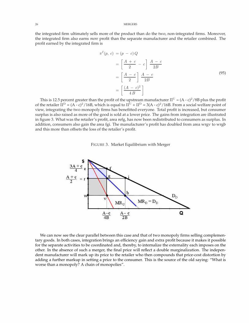
This is 12.5 percent greater than the profit of the upstream manufacturer ΠU = (A - c)2/8B plus the profitof the retailer ΠD = (A - c)2/16B, which is equal to ΠU + ΠD = 3(A - c)2/16B. From a social welfare point ofview, integrating the two monopoly firms has benefitted everyone. Total profit is increased, but consumersurplus is also raised as more of the good is sold at a lower price. The gains from integration are illustratedin figure 3. What was the retailer’s profit, area refg, has now been redistributed to consumers as surplus. Inaddition, consumers also gain the area fgi. The manufacturer’s profit has doubled from area wrgv to wrgband this more than offsets the loss of the retailer’s profit.
FIGURE 3. Market Equilibrium with Merger
We can now see the clear parallel between this case and that of two monopoly firms selling complemen-tary goods. In both cases, integration brings an efficiency gain and extra profit because it makes it possiblefor the separate activities to be coordinated and, thereby, to internalize the externality each imposes on theother. In the absence of such a merger, the final price will reflect a double marginalization. The indepen-dent manufacturer will mark up its price to the retailer who then compounds that price-cost distortion byadding a further markup in setting a price to the consumer. This is the source of the old saying: “What isworse than a monopoly? A chain of monopolies”.
MERGERS 27
One further point should be stressed in reviewing the above analysis. This is that the gains brought on byintegration hinge crucially on the fact that the pre-merger setting was one of the monopoly at both levels ofactivity, manufacture and retail. If, instead, we had started with either a competitive manufacturing sectorupstream selling to a monopoly downstream, or a monopoly stream selling to a competitive retail sector,there would be no efficiency gain to vertical integration. Price competition upstream among manufacturersleads to a wholesale price equal to marginal cost. Similarly, competition among retailers downstream bringsthe retail price equal to r. In either case, the margin of price over cost will be set to zero at one of the twolevels of activity. Hence, in these settings, no double marginalization can occur.
We should also note one additional qualification to the foregoing analysis. The benefits that the verticalmerger of an upstream and downstream monopolist assumes that the downstream firm operates underconditions of fixed input proportions. This means we have assumed that the downstream firm uses somefixed amount of the upstream firm’s product for every unit of output that the downstream firm sells. In ourexample of a producer and a downstream retailer this assumption may make sense. The retailer has to haveone unit of the manufacturer’s product for every unit it resells to its customers. Yet for other situations thisassumption is too strong. For example, if the upstream firm is a steel producer and the downstream firmis an automobile manufacturer, the steel firm’s decision to charge the car company a price, r, that includesa high markup, may induce the auto maker to switch to aluminum or perhaps fiberglass, both assumed tobe competitively supplied. In such a case, the benefits of the car company integrating backwards into thesteel market are less clear-cut. If substitution possibilities are great enough, they may be sufficient to offsetthe benefits that accrue from removal of double marginalization.
28 MERGERS
3.4. Vertical Merger to Facilitate Market Foreclosure.
3.4.1. Why market foreclosure may be important. One motive for vertical integration is foreclosure, that is, themerger of vertically related firms so that an upstream-downstream company that can either deny down-stream rivals a source of inputs, or upstream competitors a market for their products.
Consider, for example, a situation in which a motor car manufacturer decides to merge with the companythat supplies its gear boxes. This is likely to have two effects. First, other gear-box manufacturers will nolonger be able to compete for this auto maker’s business. Secondly, it is possible that the merged firmwill prefer not to sell the gear-boxes, which as a result of the merger, it now produces, to any other autocompany. The merger firm may also attempt a “price squeeze” by offering to sell its gearboxes to outsidefirms but only at exorbitant prices.1
Such market foreclosure effects of vertical mergers may so reduce competitive forces in both the upstreamand downstream markets as to totally offset the benefits from any mitigation of the double marginalizationproblem. Indeed, this is probably one of the major reasons why regulatory agencies investigate the effectsof vertical mergers. An early Alcoa case was one particularly famous instance of foreclosure. Alcoa wasaccused of maintaining a powerful market position by extracting promises from power companies not tosupply electricity—vital to the refining of aluminum—to competing aluminum producers. In addition,they were accused of employing a price squeeze by charging very high prices for aluminum ingots thatwere used by companies that competed with Alcoa in certain downstream markets, such as the aluminumsheet market.
3.4.2. Set-up of a simple foreclosure model. Assume that there is an upstream market containing nU firms anda downstream market containing nD firms. Of these firms, n are vertically integrated, so that there are nU
- n independent, non-integrated upstream suppliers and nD - n independent, non-integrated downstreamfirms. Each of the upstream units incurs a constant marginal cost cU in making the upstream product,exactly one unit of which is needed to make one unit of the downstream product. Downstream productionincurs additional marginal costs cD per unit. The products of the downstream firms are identical and bothupstream and downstream firms act as Cournot competitors. Demand for the products of the downstreamfirm is:
pD = A − BQD (96)
where QD is aggregate output of the downstream product.
3.4.3. Profit for the three types of firms. Profit for an integrated downstream firm is:
πDi = (pD − cU − cD) qDi = (A − cU − cD − BQD) qDi (97)
Profit for a non-integrated downstream firm is:
πDn = (pD − pU − cD) qDn = (A − pU − cD − B QD) qDn (98)
Profit of a non-integrated upstream firm is:
πUn = (pU − cU ) qUn (99)
1There are, in fact, a whole host of methods by which merged firms can effectively foreclose their competitors. For an illustration ofsome of these, see Krattenmaker, T., and S. Salop (1986) “Anticompetitive exclusion: raising rivals’ costs to achieve power over price,”Yale Law Journal, pp. 209-295.

MERGERS 29
where pu is the price charged by each non-integrated upstream firm for its product. These equationsindicate an immediate advantage that the integrated firms enjoy: They obtain their inputs at marginal costwhile the non-integrated firms must pay a higher price pu.
3.4.4. Implications of the model structure.i. The equations show that the integrated firms will not purchase their inputs from non-integrated
upstream suppliers. This is obvious because for any non-integrated upstream firms to stay inbusiness it is necessary that the market price cover its cost, pu > cU. However, if this is the case,then a downstream division of an integrated firm will find it cheaper to obtain its inputs from itsupstream affiliate at cost rather than buy them on the open market for price, pu .
ii. The equations can also be used to show that the integrated firms will not supply the upstreamproduct to non-integrated downstream buyers. This second result is more complex and requiresmore analysis.
3.4.5. Integrated firms will not supply the upstream product to non-integrated downstream buyers. For the non-integrated downstream firms to stay in business it is necessary that pd - pu - cD > 0, i.e., that the downstreamprice at least covers the non-integrated firms’ production cost, including the cost of upstream supplies. If,in equilibrium, the upstream division of an integrated firm is selling some of its output to a non-integrateddownstream firm it will earn a margin of pu - cU on each unit sold. If, instead, it takes this output off theoutside market and uses it itself, total output of the final product will be unaffected and so the downstreamprice will not change. But this means that the integrated firm will earn pd - cU - cD on every unit so diverted.So, if the condition for a non-integrated downstream firm to exist, pd - pu - cD > 0, is met, the marginearned on units diverted to the integrated firm’s downstream affiliate exceeds what it earns selling to theindependent downstream firm. As a result, the integrated firms will not sell their intermediate products tonon-integrated firms. In short, foreclosure happens. However, the fact that foreclosure happens is not thesame as saying that such foreclosure is harmful to consumers. To determine this, we need to identify theeffect of vertical integration and market foreclosure on the final market price.
3.4.6. Impact of foreclosure on consumers. Consider first the upstream market. Vertical integration and themarket foreclosure just described reduces the number of independent competing firms and reduces theirnumber of customers (the remaining independent downstream companies). Both factors reduce compe-tition in the market in which the upstream product is actually sold (rather than transformed internallybetween affiliates). On the other hand, these independent upstream firms are supplying downstream com-panies who are at a cost disadvantage relative to their integrated downstream competitors (they pay theprice pu rather than the fee, cU). This constrains the ability of the independent downstream firms to raisethe price to consumers. If there are “enough” independent upstream firms following a vertical merger, theanticompetitive effects of market foreclosure by having another integrated firm will be relatively minor,and should be offset by the cost-reducing effects of vertical integration. In this case, such integration willreduce the final product price and so will not necessarily be harmful to consumers. To put it another way,the regulatory authorities can be reasonably assured that a vertical merger and the market foreclosure ef-fects it has will not have detrimental effects on consumers, if there remains a reasonably larger sector ofindependent upstream suppliers.
This analysis does not take into account the potential strategic reactions of downstream (and upstream)firms whose markets are threatened by vertical mergers. Is it likely that they will stand passively by andsee their markets destroyed? One obvious reaction of a downstream firm to the threat of foreclosure by avertically integrated rival is for this firm to seek a merger with an upstream supplier. This will have theeffect of significantly increasing competitive pressures in the downstream market because the downstreamfirms’ costs are lower, particularly if firms compete in prices rather than quantities.