Missing Data Imputation Using Regression and Classification Tree Software GUIDE

Hyunshik Lee1, Dongwook Jeong2 1Westat, 1600 Research Blvd, Rockville, MD 20850

2Statistics Korea, Government Complex-Daejeon, 189 Cheongsa-ro, Seo-gu, Daejeon 35208, Republic of Korea

Abstract Loh et al. (2016 and 2017) demonstrated that the Generalized, Unbiased, Interaction Detection, and Estimation (GUIDE) software package and other classification and regression tree algorithms can be used to impute missing data. Advantages of the tree algorithms for imputation are that they are less sensitive to model assumptions because they are non-parametric in nature, and that they can more easily handle a large number of variables and potentially numerous interaction terms in the imputation model. We want to expand current knowledge of the emerging tree-based imputation technique by comparing its performance using actual data with AutoImpute, which was developed by Westat. Key Words: Tree algorithm, item missing data, imputation model, AutoImpute

1. Introduction Almost all survey data have missing value problems. Item missing values occur when certain questionnaire items are not answered or erroneous answers are wiped out. Imputation is a popular method to handle such missing value problem. Various imputation methods have been proposed and used. There are different ways of classifying imputation methods (see Kalton and Kasprzyk, 1986). One way is by whether imputed values are randomly or deterministically chosen. Widely used hot-deck imputation is a random imputation method, whereas regression (mean or ratio) imputation is deterministic. However, a common thread of these methods is the underlying assumption that the variable to be imputed (we will call it the imputation variable) has a linear relationship with auxiliary variables, which is used to build the imputation model. The missingness (nonresponse) mechanism under this assumption is so called missing at random (MAR). The crucial step to use these methods under the MAR assumption is to correctly estimate the imputation model. If the auxiliary variables are categorical, the imputation model is given in the form of cross-classified imputation cells defined by the categorical auxiliary variables. In this case, regression imputation imputes missing values by the cell mean – this is mean imputation. If missing values are filled out by a randomly chosen respondent value from the cell, this imputation method becomes hot-deck imputation. Mean and hot-deck imputation methods share the same bias property; if the MAR assumption is true, both methods are unbiased, whereas if it is not, they have the same bias. However, mean imputation is less variable (i.e., more efficient) than hot-deck imputation, while hot-deck imputation is better to maintain the distribution of the variable. The distributional form of the imputed variable can be important in more complex analysis (e.g., estimation of quantiles, regression analysis, etc.) than simple descriptive analysis (e.g., estimation of means and proportions). Furthermore, it is important to maintain

913

multivariate distributions among survey and auxiliary variables, which may be used together in multivariate analysis. This is one reason why survey variables are also used as independent variables in development of the imputation model along with any other auxiliary variables. This approach tends to include many variables, some of which have missing values themselves, not only the imputation variables. These are important aspects in developing an imputation software package. Imputation models are constructed based on parametric or semiparametric models that govern the distribution of the data. For example, AMELIA (Honaker, King, and Blackwell, 2011) assumes a multivariate normal distribution, with categorical variables converted into 0-1 dummy vectors (there is a tacit assumption of existence of an underlying continuous distribution, which can be categorized into a 0-1 dummy), and MICE (van Buuren and Groothuis-Oudshoorn, 2011) based on the methodology proposed by Raghunathan, (2004) uses linear regression for imputation of continuous and ordinal variables and polytomous logistic regression for categorical variables. AutoImpute (Judkins,1997; Krenzke et al., 2005; Piesse et al., 2005; Judkins et al., 2007, 2008) uses a semiparametric approach as it first develops GLM models, and then imputation cells are formed based on predicted values to perform hot-deck imputation. These methods cannot accept missing values in the predictor variables, and therefore, missing values must be filled out with a crude imputation method (e.g., hot-deck imputation using predetermined imputation cells) to start the process. Recently, a very different approach has been proposed, a method using the classification and regression tree (CRT) algorithm. Recently, Loh et al. (2016 and 2017) used the GUIDE package (Loh, 2002, 2009; Loh and Zhang, 2013) to do imputation with a data set having hundreds of variables with various levels of missing values. They studied imputation of a single continuous variable with the Bureau of Labor Statistics (BLS) Consumer Expenditure Data with over 600 variables, many of which have various amount of missing values. They compared the performance of GUIDE-based methods with AMELIA, MICE, and other tree-based methods using CART (Breiman et al., 1984). Their comparison metric were bias and mean squared error (MSE) of the mean estimate of the continuous variable. The GUIDE-based methods performed well and has some important advantages over other methods, notably, its capability of easily handling a large number of variables with good speed, and easily accommodating missing data in the predictor variables. More detailed discussion is given in the next section. In this study, we extend the Loh et al. (2016, 2017) study to compare GUIDE-based methods with AutoImpute (developed by Westat) for imputation of both continuous and categorical variables.

2. GUIDE-based Imputation Methods and AutoImpute 2.1 GUIDE-based Imputation Methods In general, a CRT-based method uses a classification tree for imputation of a categorical variable and a regression tree to impute a continuous or ordinal variable. The final nodes of the classification or regression tree are used as imputation cells, where we can use hot-deck imputation for both types of variables or the predicted category for the categorical variable and the predicted value (i.e., mean) for the continuous variable. Any tree algorithm can be used in this way for imputation but we prefer using GUIDE to other tree algorithms

914

for its lack of selection bias and versatility in handling missing values. The following list provides advantages of GUIDE-based methods (some of which are general to CRT-based methods but some are particular to GUIDE).

1. It is non-parametric in nature, and thus less vulnerable to model misspecifications; 2. It can easily handle many variables and interaction terms; 3. It does not suffer from selection bias; 4. It can easily handle missing values in the predictor variables; 5. It can use categorical variables with an (almost) unlimited number of categories; 6. It is fast computationally.

The first and second ones are more general to CRT-based methods. The rest are more particular to GUIDE, although some features may also be available in other CRT-algorithms. If the imputation model is perfectly correct, then methods strongly dependent on the model will perform better than any non-parametric methods. However, there is always some degree of uncertainty in the assumed model, and it would be very difficult to check the validity of every model, especially when the dataset is large with many imputation variables. In this case, a method less vulnerable to model misspecification is advantageous. Moreover, some methods such as MICE cannot handle multi-collinearity in linear regression and quasi-complete separation in logistic regression (Loh et al., 2016), whereas CRT-based methods are generally free from these problems. Interaction terms pose a considerable difficulty in developing imputation models, when many variables are involved. CRT-based methods have an important advantage over non-tree based methods in this regard. CART (Breiman et al, 1984) is known to have bias in variable selection by favoring categorical variables with many categories, whereas GUIDE does not have such a problem (Loh, 2014). So, when selecting a CRT-based imputation method for a dataset with many categorical variables, this aspect should be taken seriously. MICE and AutoImpute allow up to 32 categories, whereas CART, GUIDE, and AMELIA do not have this limitation but AMELIA converts each category by a 0-1 dummy, which tends to increase the number of variables. The selection bias problem can be serious as Loh et al. (2016) demonstrated, where CART selected the variable ‘State’ more often in the tree model than GUIDE in their study – this may cause a bias in imputed values. GUIDE treats missing values for a categorical predictor variable as another category, and for a continuous predictor variable lumps missing cases into the left node, although there are some variations depending on the situation (Loh, 2009). GUIDE also has a computational advantage as shown in Loh et al. (2016, 2017). When GUIDE is used for imputation, there are several possibilities. A tree can be built on the variable itself or on the item response status. We can use either the final nodes for hot-deck imputation or predicted values GUIDE produces. Possible methods depend on four factors: (1) whether the imputation variable (variable to be imputed) is categorical or continuous/ordinal; (2) whether the object variable of the tree algorithm is the imputation variable or the item response status of the imputation variable; (3) whether the tree algorithm is classification or regression; (4) whether the imputed value is given by the predicted value or chosen by the hot-deck method. The tree algorithm includes the random

915

classification and regression forests. We will use a coding system to describe different methods as shown below:

By combining different factors, we can devise different GUIDE-based imputation methods (GIMs), and we will use a coded method name to denote different methods such as GIM1112, where the first number indicates the first factor (imputation variable) code number, the second number indicates the second factor (object variable) code number, etc. So, GIM1112 is the method code name for hot-deck imputation performed at the final nodes of the GUIDE classification tree (GCT) for a categorical imputation variable using it as the object variable of the GCT. Some combinations are impossible. For example, GIM2112 does not exist because a classification tree cannot be formed for a continuous imputation variable as the object variable, whereas GIM2212 is feasible because the object variable is categorical even though the imputation variable is continuous. In this case, the outputs of GCT are the final nodes and the response propensities, which can be used for imputation; Hot-deck imputation can be performed at each final node for missing case in the node (this method is coded as GIM2212a) or at imputation cells formed using the propensity scores (coded as GIM2212b). Another possibility is to use the node mean to impute missing values in the node – this method is coded as GIM2211 treating node means as predicted values. In the same vein, when the GUIDE regression tree (GRT) is used, certain combinations are not feasible; in particular, the imputation variable cannot be categorical, that is, GIM1121 and GIM1122 are infeasible. When the random forest is used, we do not get tree nodes since no tree is produced, instead we get predicted values for a continuous object variable or predicted category or probability for a categorical object variable. Predicted values or categories can be directly used for imputation for both types of imputation variables. Also, the predicted values for a continuous imputation variable or predicted probabilities for a categorical imputation variable can be used to form imputation cells, where hot-deck imputation can be performed. Therefore, we can think of several feasible methods with a GUIDE classification forest (GCF) or regression forest (GRF). For a categorical imputation variable, feasible methods are GIM1131 and GIM1132, and for a continuous imputation variable, GIM2141 and GIM2142 are feasible. Choosing the response status as the object variable for either a categorical or continuous imputation variable, there are also a number of feasible methods using GCF such as GIM1232 and GIM2232, but we did not try them in this study.

Table 1: Factors and Coding System for GUIDE-based Imputation Methods

Factor (1) Imputation Variable

(2) Object Variable (3) Tree Algorithm (4) Imputation Method

Category Code Category Code Category Code Category Code Categorical 1 Imputation

Variable 1 Classification 1 Predicted 1

Continuous 2 Response Status

2 Regression 2 Hot-deck 2

Classification Forest

3

Regression Forest

4

916

The second factor determines two fundamentally different approaches to imputation. When the imputation variable is used as the object variable of the tree algorithm, the focus is on the imputation model under MAR that relates the imputation variable and other variables involved in the imputation process, whereas if the response status is used as the object variable, the focus is on building homogeneous cells with respect to the response propensity. If we are simply interested in estimating the mean, we can use inverse propensity weighting with nonmissing cases only to estimate the mean without imputing the missing values. However, our goal is not just to estimate the mean but produce a complete dataset for multiple purpose data analysis. Therefore, we do not consider weighting options in this paper. Mean estimates from imputed data are unbiased when either the imputation model is correct or the response model is correct. When a weighting method is used, a doubly-robust mean estimate for a continuous variable can be used as discussed in Loh et al. (2017), where GRT or GRF is used to obtain predicted values and GCT or GCF is used to get response propensities, and then the mean estimate is calculated by adding the inverse propensity weighted mean residuals to the sample weighted mean of predicted values. This can be changed to a doubly-robust imputation procedure by defining the imputed value for each missing case by the sum of the predicted value and a randomly selected residual (i.e., hot-deck imputed residual). Loh et al. (2017) did not consider any doubly-robust imputation procedures but a number of different methods can be conceived depending on how to form the hot-deck imputation cells. We did not study these options but leave them for future study. 2.2 AutoImpute (AI) This is an imputation software package developed in Westat, which has been used for small- and large-scale surveys (e.g., Li et al., 2008). Like AMELIA, it converts a categorical variable into (𝑙𝑙 − 1) 0-1 dummy variables that fully represent the categorical variable with 𝑙𝑙 categories. The core engine of the package is the generalized linear model (GLM) with the imputation variable as the dependent variable and all other variables (both auxiliary and survey) as predictors – this helps maintain the relationships between variables in the imputed data. Stepwise model selection is used, and the predicted values of the final model are used to form imputation cells, where hot-deck imputation is performed. It does not allow missing values in the predictors, so it starts with crudely imputed values (e.g., hot-deck imputed values with readily definable imputation cells using nonmissing categorical variables or using the entire sample as the single imputation cell). Whenever newly imputed values by AI becomes available, the crudely imputed values are replaced in GLM modeling, and this goes on a number of cycles until imputed values converge or it reaches the specified number of iterations. Imputed dummy variables created for a categorical variable are converted back to the categorical variable using a clustering algorithm. One very important feature of AI, which is not available in any other imputation packages as far as the authors know, is its capability of preserving skip patterns. Oftentimes, a survey questionnaire uses skip questions to control the response process (e.g., male respondents are asked to skip pregnancy related questions), and a dataset produced from such a questionnaire contains skip-related variables. It is nontrivial to preserve skip patterns in the imputed data (e.g., a record with the gender variable imputed to be male should have all pregnancy variables coded as inapplicable). Therefore, we would like to keep using AI as long as it performs better or comparatively with other imputation methods.

917

3. Comparisons of GUIDE-based Imputation Methods with AutoImpute (AI) 3.1 Simulation Setup We compared GUIDE-based imputation methods with AI via simulation using the 2013 Consumer Expenditure (CE) Survey data produced by the Bureau of Labor Statistics (BLS). The CE Survey has been conducted every quarter to obtain approximately 600 questionnaire items from sampled consumer units (CUs) by BLS – the sample size in 2013 was 25,822. Each variable with missing values is accompanied by a flag that indicates the missing status or top coding status as follows:

A C D T

Valid nonresponse: a response is not anticipated “Don’t know”, refusal or other type of nonresponse Valid data value Top coding applied to value

To reduce the simulation run time, we selected 61 variables including flag variables from over 600 variables and deleted cases with the flag variable equal to A or T among 61 variables, that is, cases with inapplicable (i.e., valid missing) values or top-coded values. This restriction resulted in 1,153 records. The 61 variables we used (see Appendix for the full list of them) include all 57 variables Loh et al. (2016) used in one of their various simulation setups. Among the 61 variables we selected four variables (two continuous and two categorical variables) as imputation variables, which are listed below.

• INTRDVX - Amount of income received from interest and dividends (423 missing, 36.7%)

• IRAX - Total value of all retirement accounts (426 missing, 36.9%) • DEFBENRP – Have a retirement plan (Yes/No) (65 missing, 5.6%) • EITC - Claimed an Earned Income Tax Credit on federal income tax return

(Yes/No) (27 missing, 2.3%) To create the population data for these four variables without missing values, we ran GUIDE regression forest (GRF) to obtain predicted values for continuous variables (INTRDVX and IRAX) and GUIDE classification forest (GCF) to estimate the probability of the binomial (categorical) variables (DEFBENRP and EITC) having “Yes.” Using the deciles of these predicted values or estimated probabilities, we defined 10 imputation cells to perform hot-deck imputation for missing values. Once again, we ran GCF to predict the response propensities with the response status as the object variable for each of the four imputation variables. Using the response propensities, we performed Bernoulli trials to generate missing cases for each of the four imputation variables, while leaving missing values of other variables. To this dataset with generated missing values for the four imputation variables, we applied GUIDE-based imputation methods and AutoImpute (AI). We want to focus on the imputation error by taking the census without worrying about the sampling error. We repeated this response experiment and imputation 200 times to obtain simulated performance of the imputation methods we studied. When we selected GUIDE-based methods, we used the same method for the two continuous variables (INTRDVX and IRAX) and the same method for the two categorical variables (DEFBENRP and EITC) although we could use one method for INTRDVX and another method for IRAX, and

918

similarly for categorical imputation variables. However, we mixed different methods for the two pairs of variables and selected six combinations for the study as shown in the following table.

When we defined imputation cells for hot-deck imputation using the predicted values or probabilities or response propensities, we always used deciles (i.e., ten equally divided groups). We distinguish variables, which do not need imputation even though they have missing values, from imputation variables – we call them non-imputation variables. GUIDE-based methods left missing values for them but AutoImpute imputes all non-imputation variables to make it run regardless of whether imputation is necessary or not. 3.2 Simulation results The results of the simulation are summarized in boxplots for means or proportions of the four imputation variables from 200 imputed datasets and bar chart for the root mean squared error (RMSE) of the means.

Figure 1: Boxplot of means (true mean on the red line) and bar chart of RMSEs

for INTRVDX

1,200.01,400.01,600.01,800.02,000.02,200.02,400.02,600.0

INTRDVX=2,010.1

0.0

50.0

100.0

150.0

200.0

250.0

INTRDVX

Table 2: GUIDE-based Imputation Methods Used in Simulation

Continuous Variable Categorical Variable Description Method

Name Description Method

Name CCT-HD GCT and Hot-deck GIM2212a GCT and Hot-deck GIM1112 CCT-P GCT and Predicted

(node mean) GIM2211 GCT and Predicted GIM1111

RCT-HD GRT and Hot-deck GIM2122 GCT and Hot-deck GIM1112 RCT-P GRT and Predicted GIM2121 GCT and Predicted GIM1111 RCF-HD GRF and Hot-deck GIM2142 GCF and Hot-deck GIM1132 RCF-P GRF and Predicted GIM2141 GCF and Predicted GIM1131

919

Figure 2: Boxplot of means (true mean on the red line) and bar chart of RMSEs for IRAX

Figure 3: Boxplot of means (true proportion on the red line) and bar chart of RMSEs for DEFBERNRP

150,000.0160,000.0170,000.0180,000.0190,000.0200,000.0210,000.0

CCT-

HDCC

T-P

RCT-

HDRC

T-P

RCF-

HDRC

F-P AI

IRAX=178,141.5

0.0

2,000.0

4,000.0

6,000.0

8,000.0

10,000.0

12,000.0

IRAX

0.45000

0.46000

0.47000

0.48000

0.49000

0.50000

CCT-

HD

CCT-

P

RCT-

HD

RCT-

P

RCF-

HD

RCF-

P AI

DEFBERNRP=0.47441

0.00000

0.00100

0.00200

0.00300

0.00400

0.00500

0.00600

DEFBERNRP

920

Figure 4: Boxplot of means (true proportion on the red line) and bar chart of RMSEs for EITC

We also examined the distributional conformity of imputed data with the population data by comparing the empirical distribution function (EDF) of imputed data for a continuous variable with the population distribution using the Kolmogorov–Smirnov test and the frequency distribution of imputed data for a categorical variable with the population frequency using the Chi-square test. EDF graphs shown below vividly depicts how the EDF comparisons look. The graphs are for INTRDVX, and the first one is the comparison between the imputed EDF by CCT-HD (blue line) and the population EDF (red line). The second is for the imputed EDF by CCT-P. It is clear that hot-deck imputation greatly improves the distributional conformity. This pattern is the same between RCT-HD and RCT-P (graphs are not shown).

Figure 5: EDFs of the imputed variable (blue line) INTRDVX by CCT-HD (left) and CCT-P (right) compared with the population EDF (red line)

0.020000.022000.024000.026000.028000.030000.032000.03400

CCT-

HD

CCT-

P

RCT-

HD

RCT-

P

RCF-

HD

RCF-

P AI

EITC=0.02862

0.00110

0.00115

0.00120

0.00125

0.00130

0.00135

0.00140

EITC

921

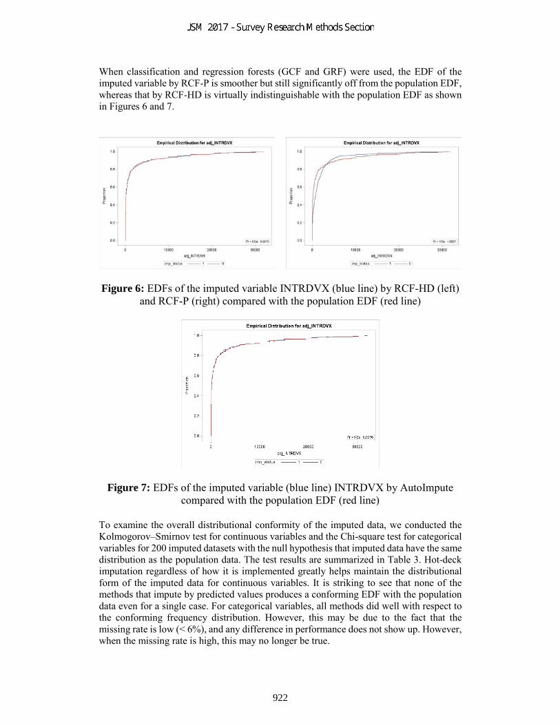
When classification and regression forests (GCF and GRF) were used, the EDF of the imputed variable by RCF-P is smoother but still significantly off from the population EDF, whereas that by RCF-HD is virtually indistinguishable with the population EDF as shown in Figures 6 and 7.

Figure 6: EDFs of the imputed variable INTRDVX (blue line) by RCF-HD (left) and RCF-P (right) compared with the population EDF (red line)

Figure 7: EDFs of the imputed variable (blue line) INTRDVX by AutoImpute compared with the population EDF (red line)

To examine the overall distributional conformity of the imputed data, we conducted the Kolmogorov–Smirnov test for continuous variables and the Chi-square test for categorical variables for 200 imputed datasets with the null hypothesis that imputed data have the same distribution as the population data. The test results are summarized in Table 3. Hot-deck imputation regardless of how it is implemented greatly helps maintain the distributional form of the imputed data for continuous variables. It is striking to see that none of the methods that impute by predicted values produces a conforming EDF with the population data even for a single case. For categorical variables, all methods did well with respect to the conforming frequency distribution. However, this may be due to the fact that the missing rate is low (< 6%), and any difference in performance does not show up. However, when the missing rate is high, this may no longer be true.

922

In terms of RMSE, hot-deck imputation based on GUIDE classification and regression forests (RCF-HD) is the best performer, followed by RCF-P in second, and AutoImpute (AI) in third. If we take the distributional conformity as another important criterion, RCF-HD and AI are virtually tied, and overall, RCF-HD is the best and followed by AI.

4. Summary and Concluding Remarks We compared GUIDE-based imputation methods with AutoImpute using simulation with the BLS Consumer Expenditure Data. The hot-deck imputation method based on GUIDE classification and regression forests (RCF-HD) performed the best in terms of MSE and distributional conformity and was followed by AutoImpute. This study demonstrated the potential of GUIDE-based (more generally tree-based) imputation methods. Nevertheless, it is difficult to generalize the results because the simulation setting is limited. So, more study is needed under systematically widely different settings in terms of the size of the dataset, missing pattern, relationship between variables, and model specification. At this stage of research, we also omitted interesting options (feasible options under GCF and GRF) and doubly-robust methods. These are also topics of a future study. Variance estimation is important for data analysis, and although we conducted a limited study in this area with mixed results (not presented in this paper), it certainly needs more study in the future.

Acknowledgements We are grateful to David Morganstein, Director of the Statistical Group, Westat for his support for this research. We also thank Keith Rust for his helpful comments, which have brought significant improvement.

Table 3: Number of Rejections of Kolmogorov–Smirnov and Chi-square Tests (n=200)

Method INTRDVX IRAX DEFBERNRP EITC CCT-HD 0 6 0 0 CCT-P 200 200 0 0 RCT-HD 0 1 0 0 RCT-P 200 200 0 0 RCF-HD 0 0 0 0 RCF-P 200 200 0 0 AI 0 1 0 0

923

References Breiman, L., Friedman, J. H., Olshen, R. A. and Stone, C. J. (1984). Classification and

Regression Trees. Wadsworth, Belmont. Honaker, J., King, G. and Blackwell, M. (2011). Amelia II: A Program for Missing Data.

Journal of Statistical Software, 45, 1-47. Judkins, D. R. (1997). Imputing for Swiss cheese patterns of missing data. Proceedings of

Statistics Canada Symposium 97, New Directions in Surveys and Censuses, 143-148. Judkins, D., Krenzke, T., Piesse, A., Fan, Z., and Haung, W.C. (2007). Preservation of skip

patterns and covariate structure through semi-parametric whole questionnaire imputation. Proceedings of the Section on Survey Research Methods of the American Statistical Association, pp. 3211-3218.

Judkins, D., Piesse, A., and Krenzke, T. (2008). Multiple Semi-parametric Imputation. Proceedings of the Section on Survey Research Methods of the American Statistical Association.

Kalton, G., and Kasprzyk, D. (1986). The treatment of missing survey data. Survey Methodology,12, 1-16.

Krenzke, T., Judkins, D., and Fan, Z. (2005). Vector imputation at Westat. Presented at Statistical Society of Canada Meetings, Saskatoon, Saskatchewan.

Li, L., Lee, H., Lo, A., and Norman, G. (2008). Imputation of Missing Data for the Pre-Elementary Education Longitudinal Study. Proceedings of the Section on Survey Research Methods of the American Statistical Association.

Loh, W. Y. (2002). Regression Trees with Unbiased Variable Selection and Interaction Detection. Statistica Sinica, 12, 361–386.

Loh, W. Y. (2009). Improving the precision of classification trees. Annals of Applied Statistics, 3, 1710–1737.

Loh, W. Y. (2014). Fifty years of classification and regression trees (with discussion). International Statistical Review, 34, 329-370.

Loh, W. Y., Eltinge, J., Cho, M. J., and Li, Y. (2016). Classification and regression tree methods for incomplete data from sample surveys. arXiv:1603.01631v1, Cornell University Library.

Loh, W. Y., Eltinge, J., Cho, M. J., and Li, Y. (2017). Classification and regression trees and forests for incomplete data from sample surveys. (to appear in Statistica Sinica).

Loh, W. Y. and Zheng, W. (2013). Regression trees for longitudinal and multiresponse data. Annals of Applied Statistics 7 495-522.

Piesse, A., Judkins, D., and Fan, Z. (2005). Item imputation made easy. Proceedings of the Section on Survey Research Methods of the American Statistical Association, pp. 3476-3479.

Raghunathan, T. E. (2004). What do we do with missing data? Some options for analysis of incomplete data. Annual Review of Public Health, 25, 99-117.

van Buuren, S. and Groothuis-Oudshoorn, K. (2011). mice: Multivariate Imputation by Chained Equations in R. Journal of Statistical Software, 45, 1–67.

924

Appendix

Table A-1. Description of 61 Variables Selected from Consumer Expenditure Survey Data for Simulation

No Variable Name Variable Description Missing rate

1 NEWID New Identification Number 0.0% 2 BLS_URBN Urban/Rural 0.0%

3 ETOTALP Total outlays last quarter, sum of outlays from all major expenditure categories.

0.0%

4 PROPTXPQ Property taxes last quarter 0.0% 5 PSU Primary Sampling Unit 55.3% 6 REGION Region 0.8%

7 STATE The 2010 Federal information processing standard state code

10.6%

8 AGE_REF Age of reference person 0.0% 9 AGE_REF_ Flag for AGE_REF 0.0%

10 AGE2 Age of spouse 39.5% 11 AGE2_ Flag for AGE2 0.0% 12 BATHRMQ Number of complete baths in this unit 0.5% 13 BATHRMQ_ Flag for BATHRMQ 0.0% 14 BEDROOMQ Number of bedrooms in CU 0.6% 15 BEDR_OMQ Flag for BEDROOMQ 0.0%

16 BUILDING Which of these descriptions from the list best describes this building?

0.0%

17 CUTENURE Housing tenure 0.0%

18 EARNCOMP Indicates which combinations of members of a CU are income earners

0.0%

19 EDUC_REF Education of reference person 0.0%

20

ERANKH

Complete income reporters of the total population are ranked in ascending order according to the level of total expenditures. Total expenditures is based on ERANKMTH. The value is a number between 0 and 1. (A detailed definition appears in the database)

9.5%

21 ERANKH_ Flag for ERANKH 0.0%

22

FAM_TYPE

Family Type based on Relationship of members to reference person. "Own" children are sons and daughters children including step children and adopted children

0.0%

23

FJSSDEDX

Portion of family income paid to Social Security during the past 12 months Sum of (JSSDEDX) across all members

0.0%

24 FJSS_EDX Flag for FJSSDEDX 0.0%

25

FRRETIRX

Total amount received from Social Security benefits and Railroad Benefit checks prior to deductions for medical insurance and Medicare FRRETIRX= Sum SOCRRX for all CU members

0.0%

26

INC_RANK

Weighted cumulative percent ranking based on total current income before taxes (for complete income reporters)

9.5%

27 INC__ANK Flag for INC_RANK 0.0%

28 INC_HRS1 Number of hours usually worked per week by reference person

38.3%

29 INC__RS1 Flag for INC_HRS1 0.0%

925

No Variable Name Variable Description Missing rate

30 INCNONW1 Reason reference person did not work during the past 12 months

61.7%

31 INCN_NW1 Flag for INCNONW1 0.0% 32

INCOMEY1

Employer from which reference person received the most earnings in past 12 months

38.3%

33 INCO_EY1 Flag for INCOMEY1 0.0%

34

LIQUIDX

LIQUIDXAs of today, what is the total value of all checking, savings, money market accounts, and certificated of deposit or CDs you have?

34.7%

35 LIQUIDX_ Flag for LIQUIDX 0.0% 36 MARITAL1 Marital status of reference person 0.0% 37 NO_EARNR Number of CU members reported as income earners 0.0% 38 NUM_AUTO Total number of owned cars 0.0%

39

OCCUCOD1

The job in which reference person received the most earnings during the past 12 months best fits the following category.

38.3%

40 OCCU_OD1 Flag for OCCUCOD1 0.0%

41 PERSOT64 Number of persons over 64 SUM OF MEMBERS WHERE AGE > 64 BY CU

0.0%

42 POV_CY CU below/not below the current year's poverty threshold? 9.7% 43 POV_CY_ Flag for POV_CY 0.0% 44 POV_PY Is your CU below the prior year's poverty threshold? 9.7% 45 POV_PY_ Flag for POV_PY 0.0% 46 REF_RACE Race of reference person 0.0%

47

RENTEQVX

If someone were to rent your home today, how much do you think it would rent for monthly, unfurnished and without utilities?

13.4%

48 RENT_QVX Flag for RENTEQVX 0.0% 49 RESPSTAT Completeness of income response status by code 0.0% 50

ROOMSQ

Number of rooms in CU living quarters, including finished living areas, excluding all baths

0.7%

51 ROOMSQ_ Flag for ROOMSQ 0.0% 52 SEX_REF Sex of reference person 0.0% 53

ST_HOUS

Are these living quarters presently used as student housing by a college or university?

0.0%

54 INTRDVX Amount of income received from interest and dividends 36.7% 55 INTRDVX_ Flag for INTRDVX 0.0%

56

IRAX

As of today, what is the total value of all retirement accounts, such as 401(k) s, IRAs, and Thrift Savings Plans that you own?

36.9%

57 IRAX_ Flag for IRAX 0.0%

58 DEFBENRP Do you have a defined retirement plan, such as a pension, from an employer?

5.6%

59 DEFB_NRP Flag for DEFBENRP 0.0% 60

EITC

During the past 12 months, did you claim an Earned Income Tax Credit on your federal income tax return?

2.3%

61 EITC_ Flag for EITC 0.0%

926