practical imputation of missing data
TRANSCRIPT

Dealing with Missing Survey Data
A Short Course in Practical Applications of Imputation
Mansour Fahimi, Ph.D.VP, Statistical Research Services
American Association for Public Opinion Research (AAPOR)Phoenix, Arizona
May 11, 2011
Darryl CreelResearch Statistician

Course Outline
Sources of Missing Data
Why Imputation?
Non-stochastic Methods
Stochastic Methods
Special Topics and Software Packages:
Weighted Sequential Hot-Deck Imputation
Multiple Imputation
Multivariate (Vector) Imputation
Imputation Diagnostics2

Course Structure
Introduction & Background:
2:30 – 3:30
Non-Stochastic and Stochastic Methods:
3:45 – 4:45
Special Topics and Software Packages:
5:00 – 6:00
3

Introduction & Background
We are all here for a spell;get all the good laughs you can.
Will Rogers
4
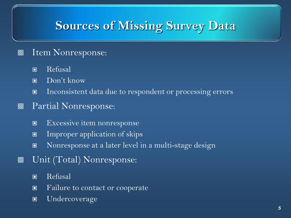
Sources of Missing Survey Data
Item Nonresponse:
Refusal
Don’t know
Inconsistent data due to respondent or processing errors
Partial Nonresponse:
Excessive item nonresponse
Improper application of skips
Nonresponse at a later level in a multi-stage design
Unit (Total) Nonresponse:
Refusal
Failure to contact or cooperate
Undercoverage5
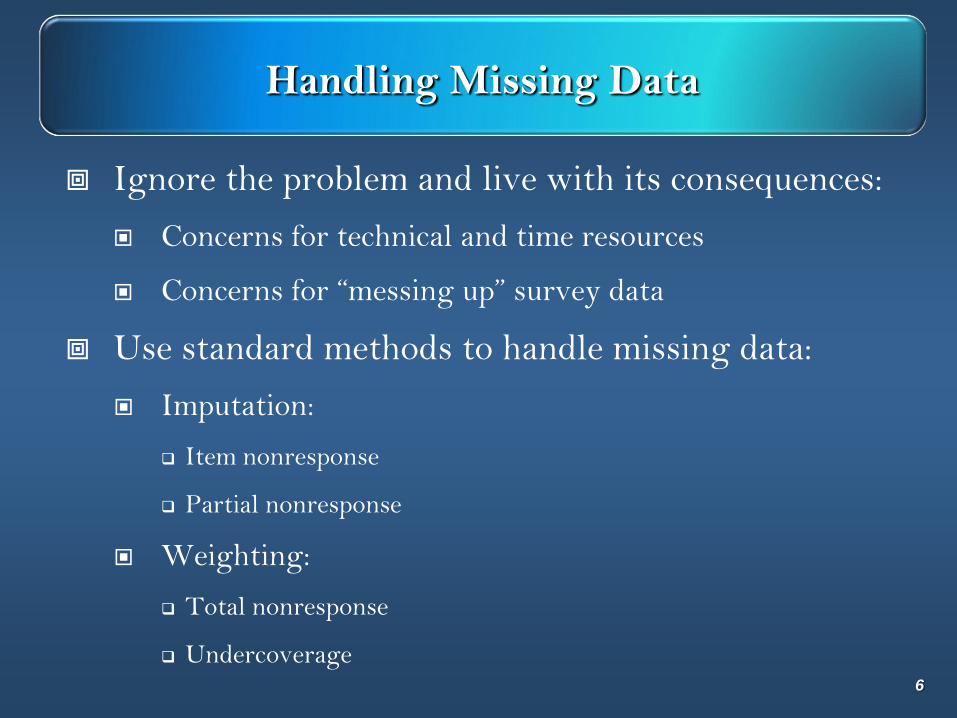
Handling Missing Data
Ignore the problem and live with its consequences:
Concerns for technical and time resources
Concerns for “messing up” survey data
Use standard methods to handle missing data:
Imputation:
Item nonresponse
Partial nonresponse
Weighting:
Total nonresponse
Undercoverage6
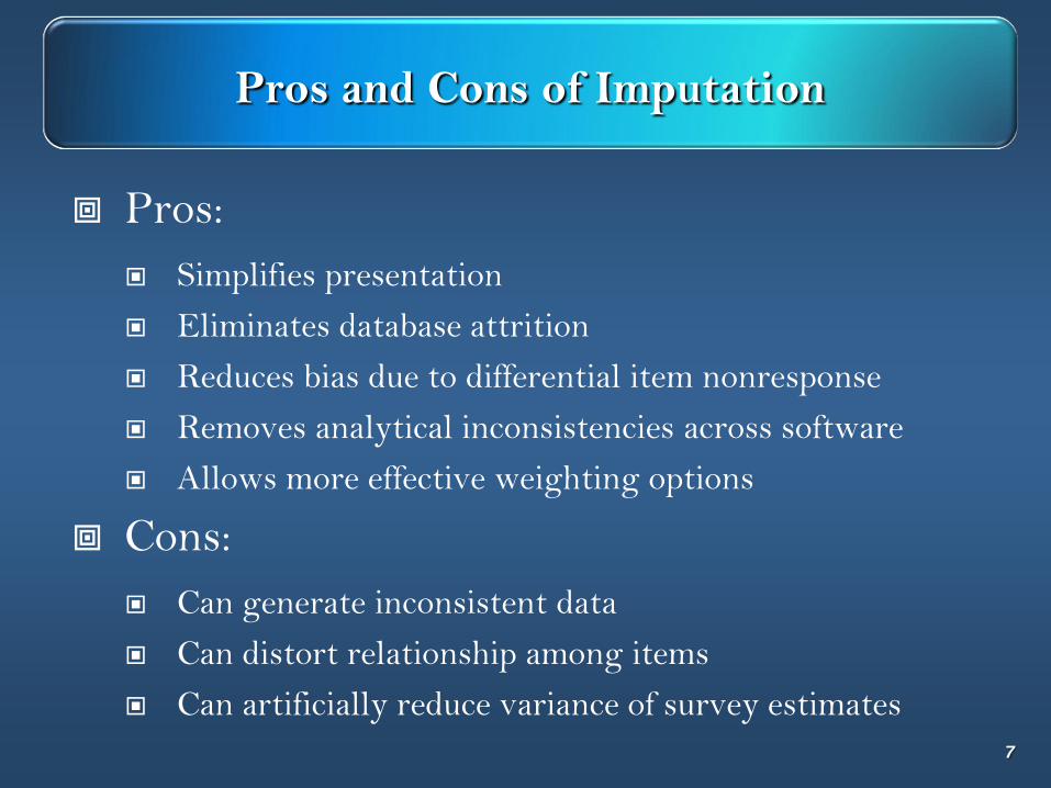
Pros and Cons of Imputation
Pros:
Simplifies presentation
Eliminates database attrition
Reduces bias due to differential item nonresponse
Removes analytical inconsistencies across software
Allows more effective weighting options
Cons:
Can generate inconsistent data
Can distort relationship among items
Can artificially reduce variance of survey estimates
7
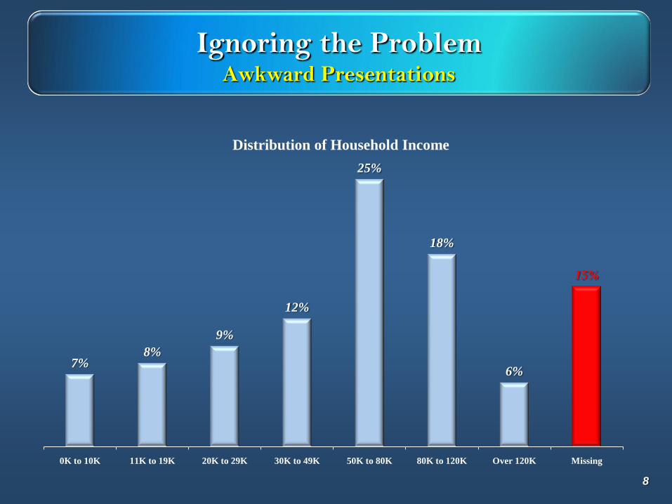
Ignoring the ProblemAwkward Presentations
7%8%
9%
12%
25%
18%
6%
15%
0K to 10K 11K to 19K 20K to 29K 30K to 49K 50K to 80K 80K to 120K Over 120K Missing
Distribution of Household Income
8
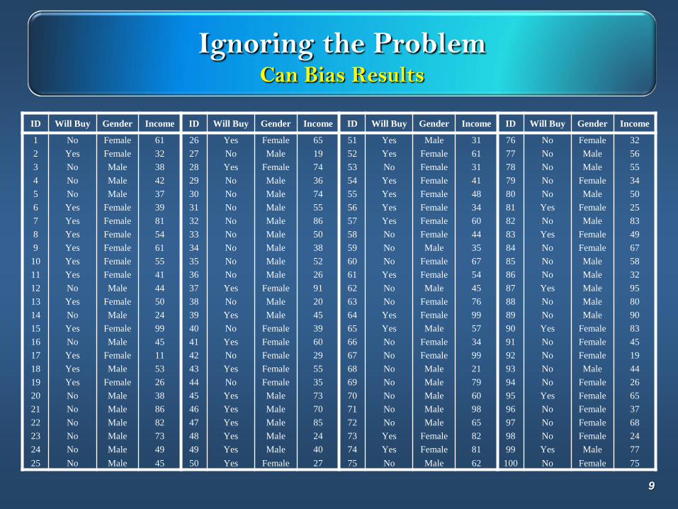
Ignoring the ProblemCan Bias Results
9
ID Will Buy Gender Income ID Will Buy Gender Income ID Will Buy Gender Income ID Will Buy Gender Income
1 No Female 61 26 Yes Female 65 51 Yes Male 31 76 No Female 32
2 Yes Female 32 27 No Male 19 52 Yes Female 61 77 No Male 56
3 No Male 38 28 Yes Female 74 53 No Female 31 78 No Male 55
4 No Male 42 29 No Male 36 54 Yes Female 41 79 No Female 34
5 No Male 37 30 No Male 74 55 Yes Female 48 80 No Male 50
6 Yes Female 39 31 No Male 55 56 Yes Female 34 81 Yes Female 25
7 Yes Female 81 32 No Male 86 57 Yes Female 60 82 No Male 83
8 Yes Female 54 33 No Male 50 58 No Female 44 83 Yes Female 49
9 Yes Female 61 34 No Male 38 59 No Male 35 84 No Female 67
10 Yes Female 55 35 No Male 52 60 No Female 67 85 No Male 58
11 Yes Female 41 36 No Male 26 61 Yes Female 54 86 No Male 32
12 No Male 44 37 Yes Female 91 62 No Male 45 87 Yes Male 95
13 Yes Female 50 38 No Male 20 63 No Female 76 88 No Male 80
14 No Male 24 39 Yes Male 45 64 Yes Female 99 89 No Male 90
15 Yes Female 99 40 No Female 39 65 Yes Male 57 90 Yes Female 83
16 No Male 45 41 Yes Female 60 66 No Female 34 91 No Female 45
17 Yes Female 11 42 No Female 29 67 No Female 99 92 No Female 19
18 Yes Male 53 43 Yes Female 55 68 No Male 21 93 No Male 44
19 Yes Female 26 44 No Female 35 69 No Male 79 94 No Female 26
20 No Male 38 45 Yes Male 73 70 No Male 60 95 Yes Female 65
21 No Male 86 46 Yes Male 70 71 No Male 98 96 No Female 37
22 No Male 82 47 Yes Male 85 72 No Male 65 97 No Female 68
23 No Male 73 48 Yes Male 24 73 Yes Female 82 98 No Female 24
24 No Male 49 49 Yes Male 40 74 Yes Female 81 99 Yes Male 77
25 No Male 45 50 Yes Female 27 75 No Male 62 100 No Female 75
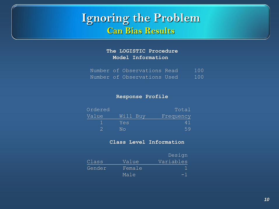
Ignoring the ProblemCan Bias Results
The LOGISTIC Procedure
Model Information
Number of Observations Read 100
Number of Observations Used 100
Response Profile
Ordered Total
Value Will Buy Frequency
1 Yes 41
2 No 59
Class Level Information
Design
Class Value Variables
Gender Female 1
Male -1
10
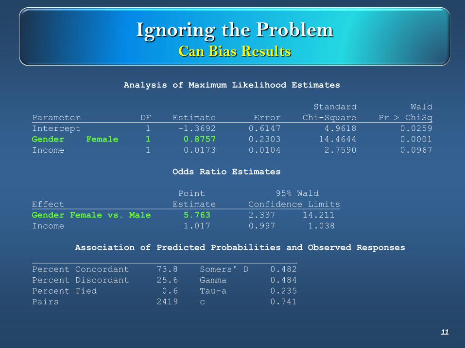
Ignoring the ProblemCan Bias Results
Analysis of Maximum Likelihood Estimates
Standard Wald
Parameter DF Estimate Error Chi-Square Pr > ChiSq
Intercept 1 -1.3692 0.6147 4.9618 0.0259
Gender Female 1 0.8757 0.2303 14.4644 0.0001
Income 1 0.0173 0.0104 2.7590 0.0967
Odds Ratio Estimates
Point 95% Wald
Effect Estimate Confidence Limits
Gender Female vs. Male 5.763 2.337 14.211
Income 1.017 0.997 1.038
Association of Predicted Probabilities and Observed Responses
_________________________________________________
Percent Concordant 73.8 Somers' D 0.482
Percent Discordant 25.6 Gamma 0.484
Percent Tied 0.6 Tau-a 0.235
Pairs 2419 c 0.741
11
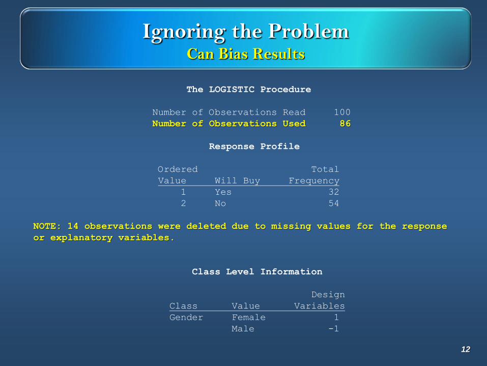
Ignoring the ProblemCan Bias Results
The LOGISTIC Procedure
Number of Observations Read 100
Number of Observations Used 86
Response Profile
Ordered Total
Value Will Buy Frequency
1 Yes 32
2 No 54
NOTE: 14 observations were deleted due to missing values for the response
or explanatory variables.
Class Level Information
Design
Class Value Variables
Gender Female 1
Male -1
12
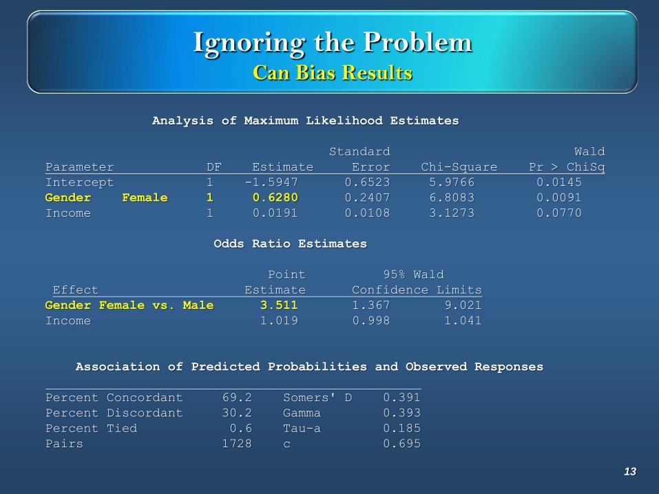
Ignoring the ProblemCan Bias Results
Analysis of Maximum Likelihood Estimates
Standard Wald
Parameter DF Estimate Error Chi-Square Pr > ChiSq
Intercept 1 -1.5947 0.6523 5.9766 0.0145
Gender Female 1 0.6280 0.2407 6.8083 0.0091
Income 1 0.0191 0.0108 3.1273 0.0770
Odds Ratio Estimates
Point 95% Wald
Effect Estimate Confidence Limits
Gender Female vs. Male 3.511 1.367 9.021
Income 1.019 0.998 1.041
Association of Predicted Probabilities and Observed Responses
_________________________________________________
Percent Concordant 69.2 Somers' D 0.391
Percent Discordant 30.2 Gamma 0.393
Percent Tied 0.6 Tau-a 0.185
Pairs 1728 c 0.695
13
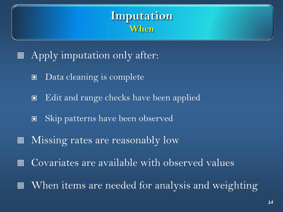
ImputationWhen
Apply imputation only after:
Data cleaning is complete
Edit and range checks have been applied
Skip patterns have been observed
Missing rates are reasonably low
Covariates are available with observed values
When items are needed for analysis and weighting
14
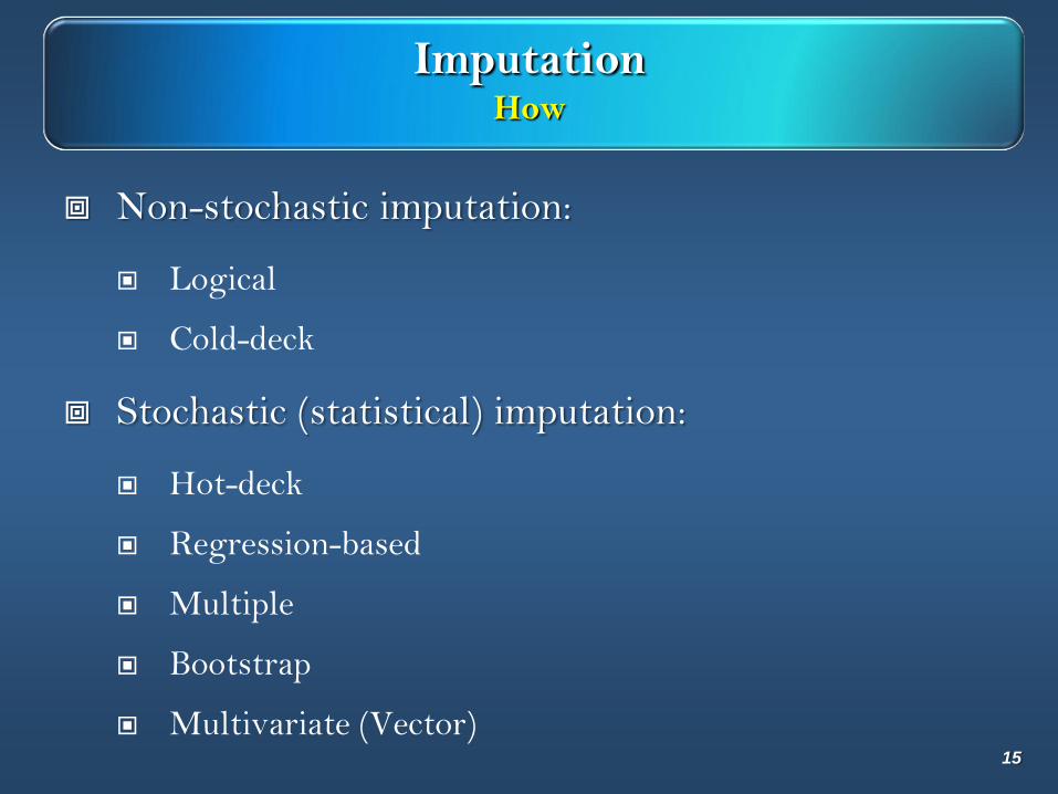
ImputationHow
Non-stochastic imputation:
Logical
Cold-deck
Stochastic (statistical) imputation:
Hot-deck
Regression-based
Multiple
Bootstrap
Multivariate (Vector)15
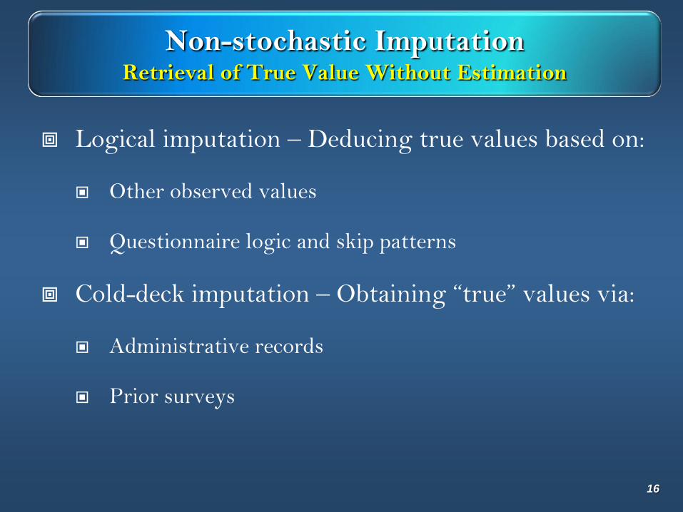
Non-stochastic ImputationRetrieval of True Value Without Estimation
Logical imputation – Deducing true values based on:
Other observed values
Questionnaire logic and skip patterns
Cold-deck imputation – Obtaining “true” values via:
Administrative records
Prior surveys
16
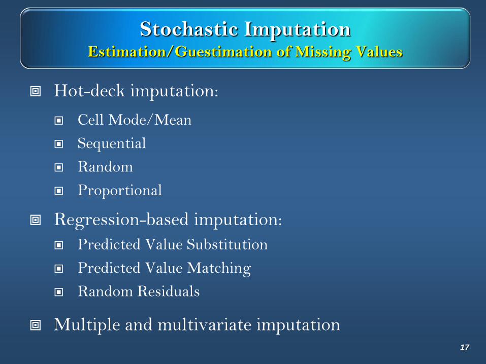
Stochastic ImputationEstimation/Guestimation of Missing Values
Hot-deck imputation:
Cell Mode/Mean
Sequential
Random
Proportional
Regression-based imputation:
Predicted Value Substitution
Predicted Value Matching
Random Residuals
Multiple and multivariate imputation17
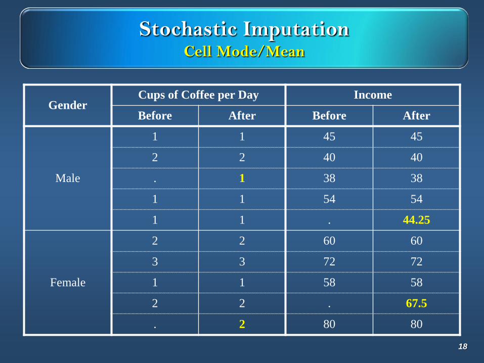
Stochastic ImputationCell Mode/Mean
GenderCups of Coffee per Day Income
Before After Before After
Male
1 1 45 45
2 2 40 40
. 1 38 38
1 1 54 54
1 1 . 44.25
Female
2 2 60 60
3 3 72 72
1 1 58 58
2 2 . 67.5
. 2 80 80
18
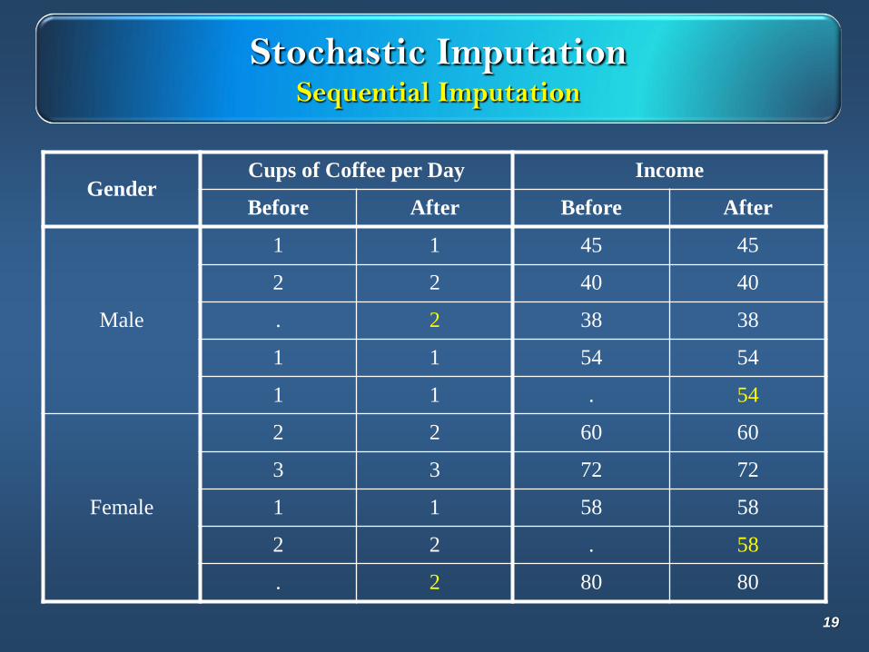
Stochastic ImputationSequential Imputation
GenderCups of Coffee per Day Income
Before After Before After
Male
1 1 45 45
2 2 40 40
. 2 38 38
1 1 54 54
1 1 . 54
Female
2 2 60 60
3 3 72 72
1 1 58 58
2 2 . 58
. 2 80 80
19
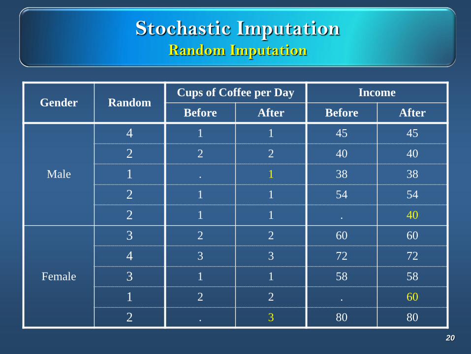
Stochastic ImputationRandom Imputation
Gender RandomCups of Coffee per Day Income
Before After Before After
Male
4 1 1 45 45
2 2 2 40 40
1 . 1 38 38
2 1 1 54 54
2 1 1 . 40
Female
3 2 2 60 60
4 3 3 72 72
3 1 1 58 58
1 2 2 . 60
2 . 3 80 80
20
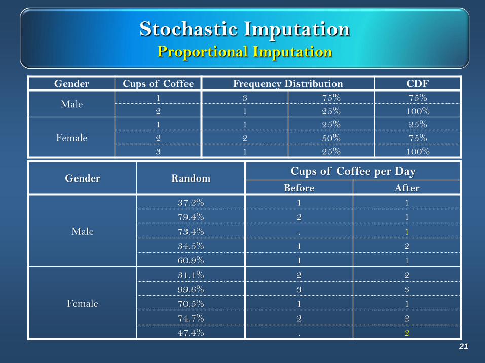
Stochastic ImputationProportional Imputation
Gender Cups of Coffee Frequency Distribution CDF
Male1 3 75% 75%
2 1 25% 100%
Female
1 1 25% 25%
2 2 50% 75%
3 1 25% 100%
Gender RandomCups of Coffee per Day
Before After
Male
37.2% 1 1
79.4% 2 1
73.4% . 1
34.5% 1 2
60.9% 1 1
Female
31.1% 2 2
99.6% 3 3
70.5% 1 1
74.7% 2 2
47.4% . 2
21
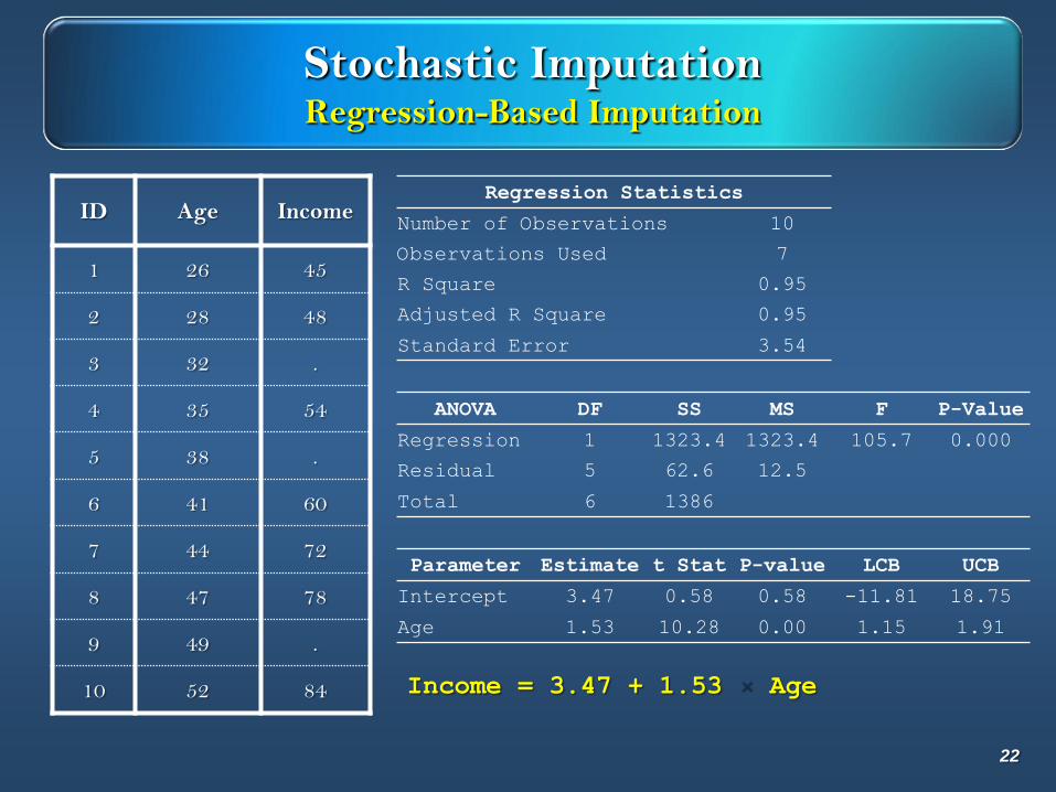
Stochastic ImputationRegression-Based Imputation
ID Age Income
1 26 45
2 28 48
3 32 .
4 35 54
5 38 .
6 41 60
7 44 72
8 47 78
9 49 .
10 52 84
Regression Statistics
Number of Observations 10
Observations Used 7
R Square 0.95
Adjusted R Square 0.95
Standard Error 3.54
ANOVA DF SS MS F P-Value
Regression 1 1323.4 1323.4 105.7 0.000
Residual 5 62.6 12.5
Total 6 1386
Parameter Estimate t Stat P-value LCB UCB
Intercept 3.47 0.58 0.58 -11.81 18.75
Age 1.53 10.28 0.00 1.15 1.91
Income = 3.47 + 1.53 Age
22
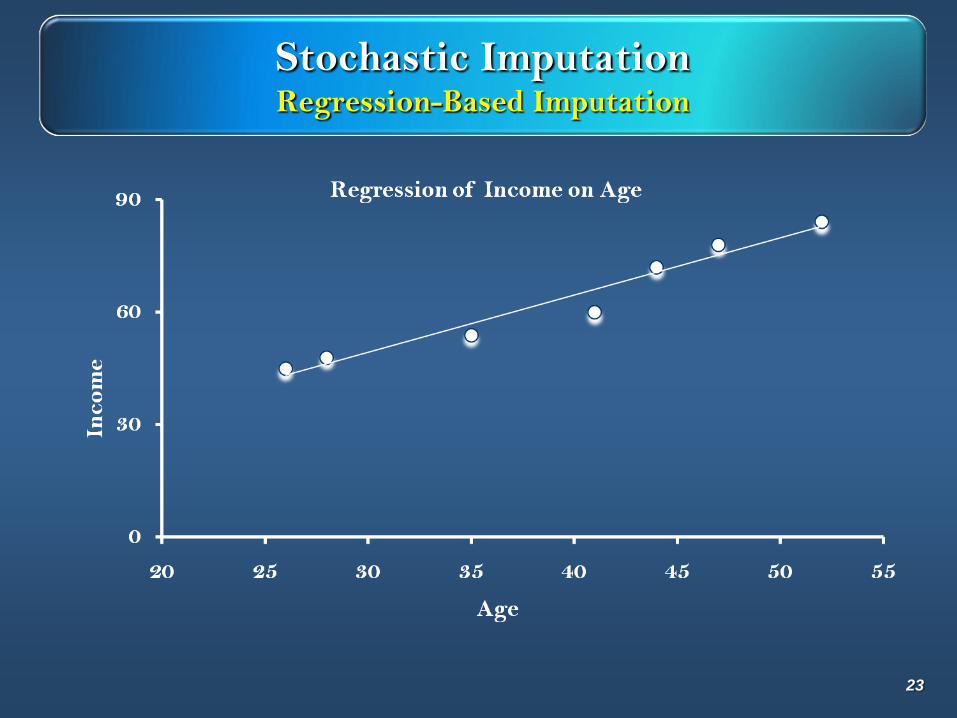
Stochastic ImputationRegression-Based Imputation
23
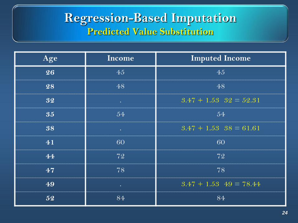
Regression-Based ImputationPredicted Value Substitution
Age Income Imputed Income
26 45 45
28 48 48
32 . 3.47 + 1.53 32 = 52.31
35 54 54
38 . 3.47 + 1.53 38 = 61.61
41 60 60
44 72 72
47 78 78
49 . 3.47 + 1.53 49 = 78.44
52 84 84
24
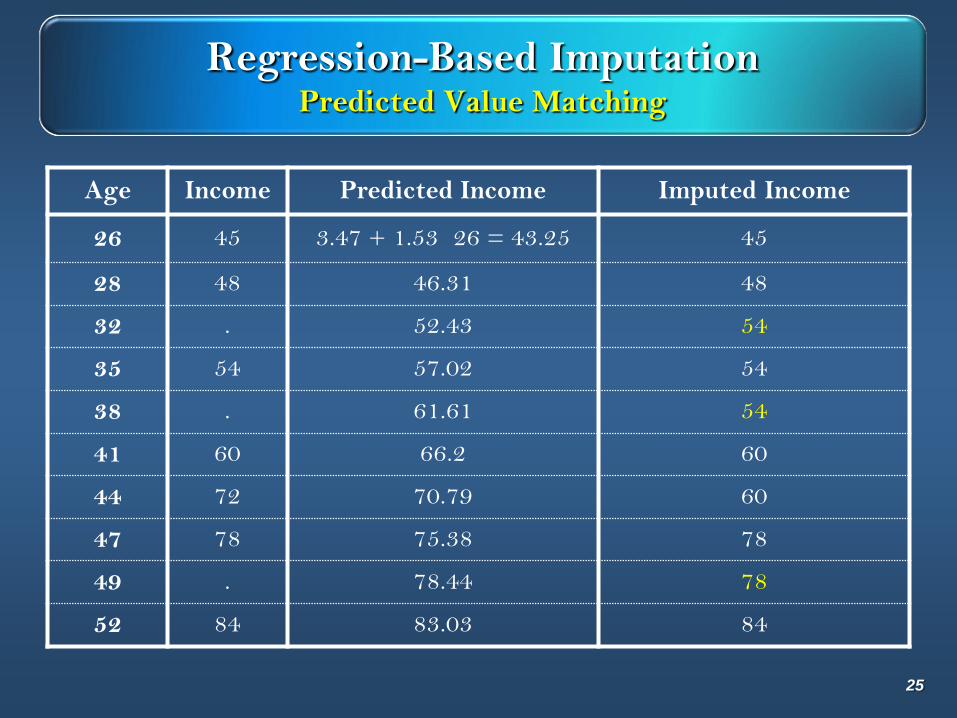
Regression-Based ImputationPredicted Value Matching
Age Income Predicted Income Imputed Income
26 45 3.47 + 1.53 26 = 43.25 45
28 48 46.31 48
32 . 52.43 54
35 54 57.02 54
38 . 61.61 54
41 60 66.2 60
44 72 70.79 60
47 78 75.38 78
49 . 78.44 78
52 84 83.03 84
25
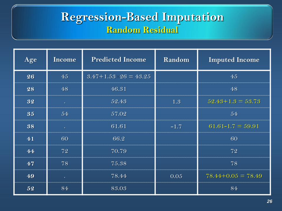
Regression-Based ImputationRandom Residual
Age Income Predicted Income Random Imputed Income
26 45 3.47+1.53 26 = 43.25 45
28 48 46.31 48
32 . 52.43 1.3 52.43+1.3 = 53.73
35 54 57.02 54
38 . 61.61 -1.7 61.61-1.7 = 59.91
41 60 66.2 60
44 72 70.79 72
47 78 75.38 78
49 . 78.44 0.05 78.44+0.05 = 78.49
52 84 83.03 84
26
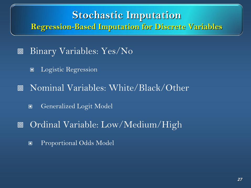
Stochastic ImputationRegression-Based Imputation for Discrete Variables
Binary Variables: Yes/No
Logistic Regression
Nominal Variables: White/Black/Other
Generalized Logit Model
Ordinal Variable: Low/Medium/High
Proportional Odds Model
27
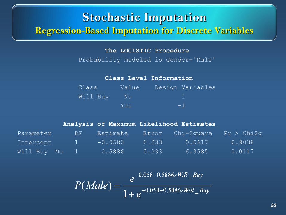
Stochastic ImputationRegression-Based Imputation for Discrete Variables
The LOGISTIC Procedure
Probability modeled is Gender='Male'
Class Level Information
Class Value Design Variables
Will_Buy No 1
Yes -1
Analysis of Maximum Likelihood Estimates
Parameter DF Estimate Error Chi-Square Pr > ChiSq
Intercept 1 -0.0580 0.233 0.0617 0.8038
Will_Buy No 1 0.5886 0.233 6.3585 0.0117
28
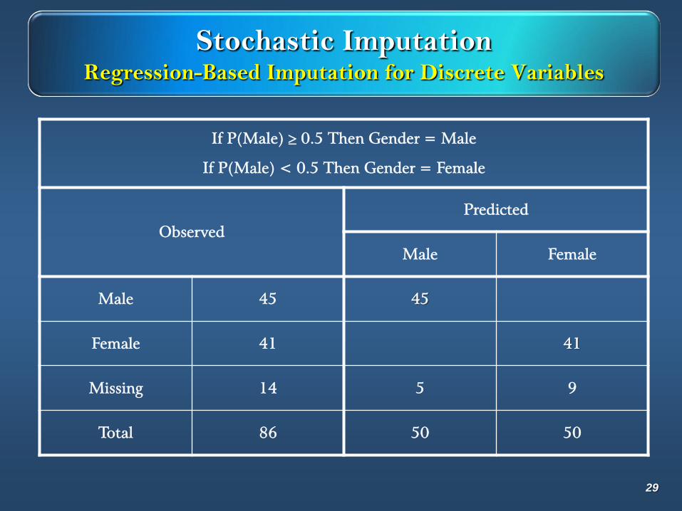
Stochastic ImputationRegression-Based Imputation for Discrete Variables
If P(Male) 0.5 Then Gender = Male
If P(Male) < 0.5 Then Gender = Female
Observed
Predicted
Male Female
Male 45 45
Female 41 41
Missing 14 5 9
Total 86 50 50
29
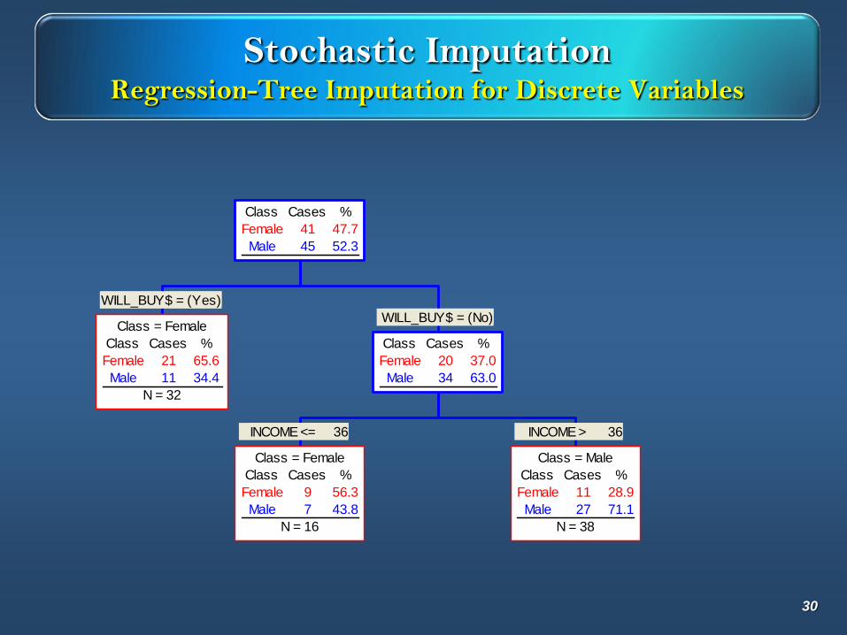
Stochastic ImputationRegression-Tree Imputation for Discrete Variables
WILL_BUY$ = (Yes)
Class = Female
Class Cases %
Female 21 65.6
Male 11 34.4
N = 32
INCOME <= 36
Class = Female
Class Cases %
Female 9 56.3
Male 7 43.8
N = 16
INCOME > 36
Class = Male
Class Cases %
Female 11 28.9
Male 27 71.1
N = 38
WILL_BUY$ = (No)
Class Cases %
Female 20 37.0
Male 34 63.0
Class Cases %
Female 41 47.7
Male 45 52.3
30
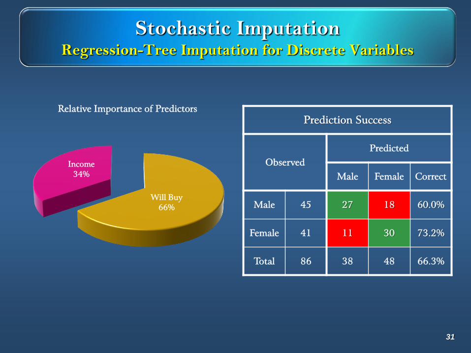
Stochastic ImputationRegression-Tree Imputation for Discrete Variables
Will Buy
66%
Income
34%
Relative Importance of Predictors
Prediction Success
Observed
Predicted
Male Female Correct
Male 45 27 18 60.0%
Female 41 11 30 73.2%
Total 86 38 48 66.3%
31
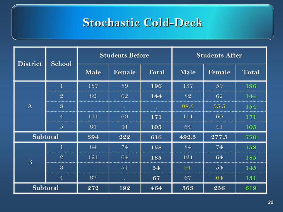
Stochastic Cold-Deck
District School
Students Before Students After
Male Female Total Male Female Total
A
1 137 59 196 137 59 196
2 82 62 144 82 62 144
3 . . . 98.5 55.5 154
4 111 60 171 111 60 171
5 64 41 105 64 41 105
Subtotal 394 222 616 492.5 277.5 770
B
1 84 74 158 84 74 158
2 121 64 185 121 64 185
3 . 54 54 91 54 145
4 67 . 67 67 64 131
Subtotal 272 192 464 363 256 619
32
Special Topics and Software Packages
Everything should be made as simple as possible, but not simpler.
Einstein
33
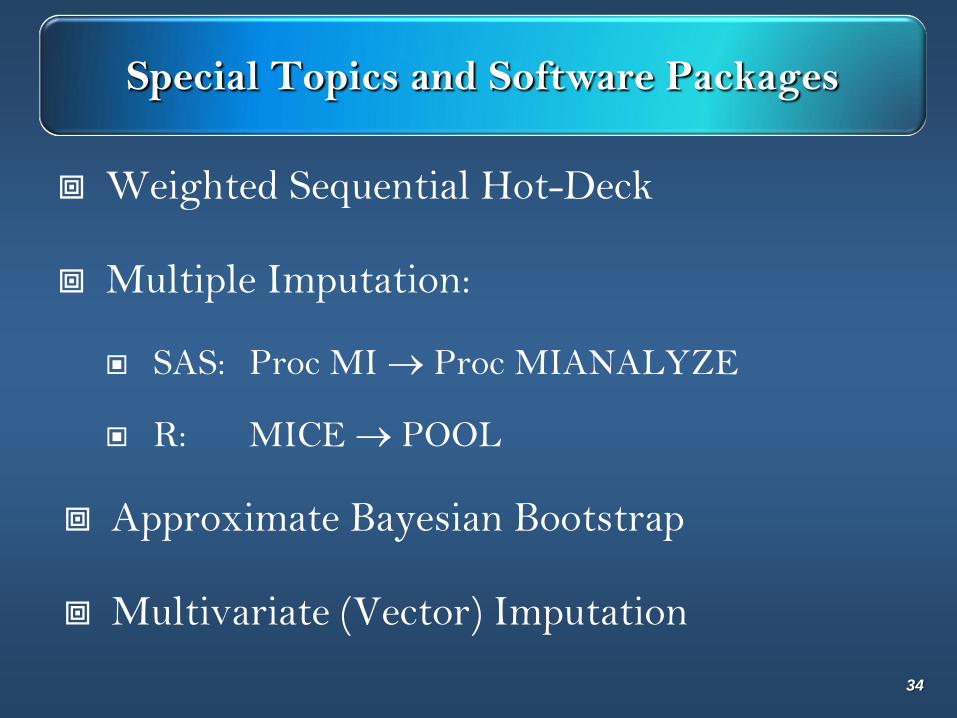
Special Topics and Software Packages
Weighted Sequential Hot-Deck
Multiple Imputation:
SAS: Proc MI Proc MIANALYZE
R: MICE POOL
Approximate Bayesian Bootstrap
Multivariate (Vector) Imputation
34
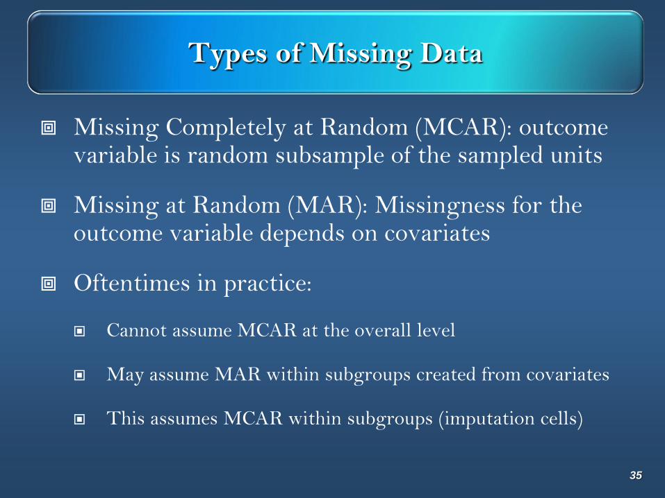
Types of Missing Data
Missing Completely at Random (MCAR): outcome variable is random subsample of the sampled units
Missing at Random (MAR): Missingness for the outcome variable depends on covariates
Oftentimes in practice:
Cannot assume MCAR at the overall level
May assume MAR within subgroups created from covariates
This assumes MCAR within subgroups (imputation cells)
35
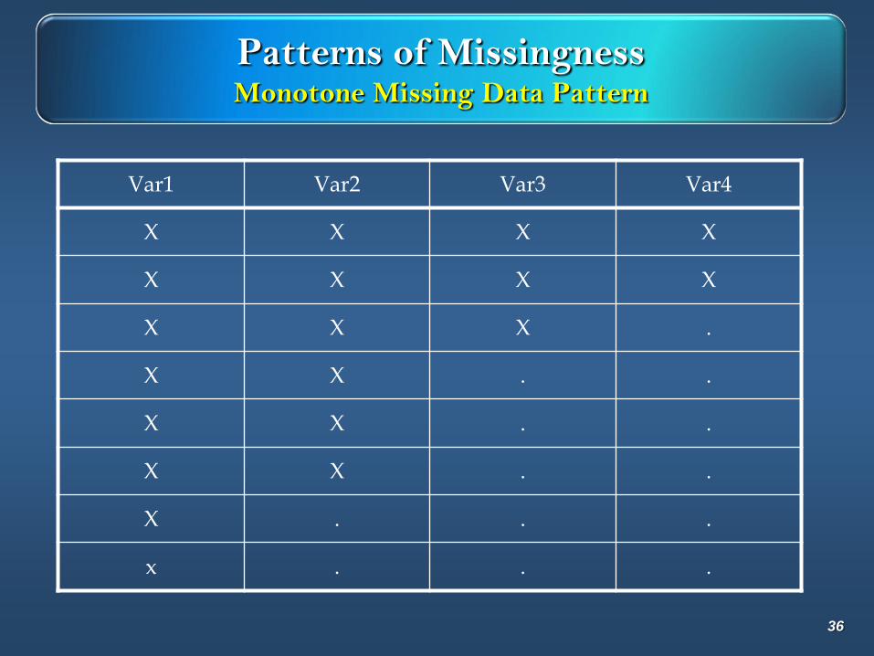
Patterns of MissingnessMonotone Missing Data Pattern
Var1 Var2 Var3 Var4
X X X X
X X X X
X X X .
X X . .
X X . .
X X . .
X . . .
x . . .
36

Patterns of MissingnessSwiss Cheese Missing Data Pattern
Var1 Var2 Var3 Var4
X . X X
. X X X
X . X .
. X . X
X X X X
X X . .
X . X .
X . . X
37
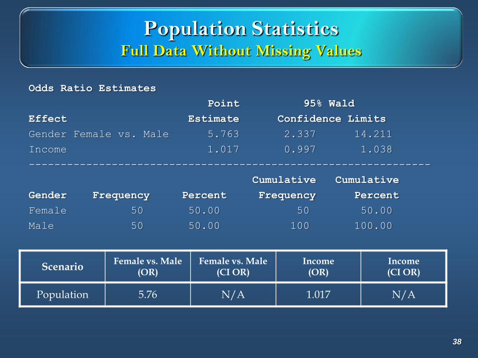
Population StatisticsFull Data Without Missing Values
Odds Ratio Estimates
Point 95% Wald
Effect Estimate Confidence Limits
Gender Female vs. Male 5.763 2.337 14.211
Income 1.017 0.997 1.038
---------------------------------------------------------------
Cumulative Cumulative
Gender Frequency Percent Frequency Percent
Female 50 50.00 50 50.00
Male 50 50.00 100 100.00
38
ScenarioFemale vs. Male
(OR)Female vs. Male
(CI OR)Income
(OR)Income (CI OR)
Population 5.76 N/A 1.017 N/A
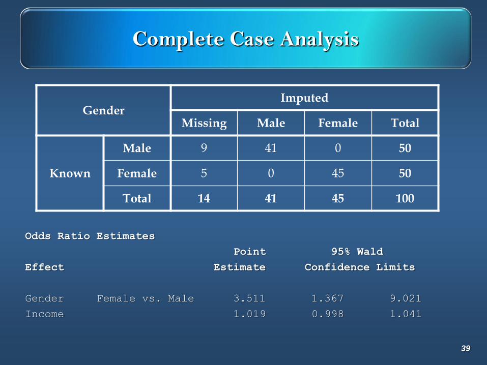
Complete Case Analysis
Odds Ratio Estimates
Point 95% Wald
Effect Estimate Confidence Limits
Gender Female vs. Male 3.511 1.367 9.021
Income 1.019 0.998 1.041
39
GenderImputed
Missing Male Female Total
Known
Male 9 41 0 50
Female 5 0 45 50
Total 14 41 45 100
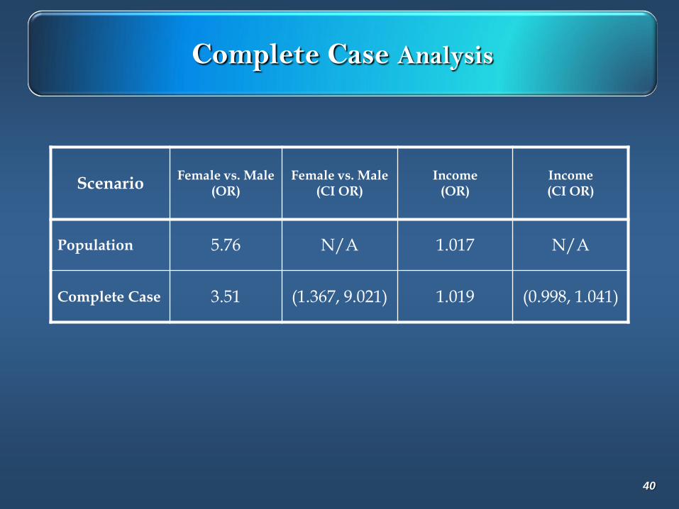
Complete Case Analysis
ScenarioFemale vs. Male
(OR)Female vs. Male
(CI OR)Income
(OR)Income (CI OR)
Population 5.76 N/A 1.017 N/A
Complete Case 3.51 (1.367, 9.021) 1.019 (0.998, 1.041)
40
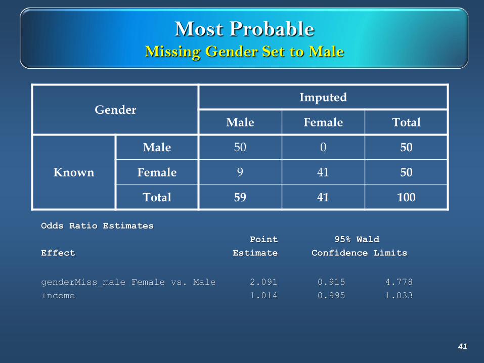
Most ProbableMissing Gender Set to Male
41
GenderImputed
Male Female Total
Known
Male 50 0 50
Female 9 41 50
Total 59 41 100
Odds Ratio Estimates
Point 95% Wald
Effect Estimate Confidence Limits
genderMiss_male Female vs. Male 2.091 0.915 4.778
Income 1.014 0.995 1.033
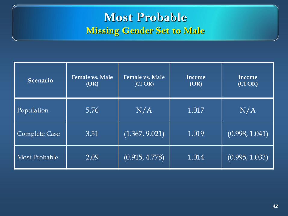
Most ProbableMissing Gender Set to Male
ScenarioFemale vs. Male
(OR)Female vs. Male
(CI OR)Income
(OR)Income (CI OR)
Population 5.76 N/A 1.017 N/A
Complete Case 3.51 (1.367, 9.021) 1.019 (0.998, 1.041)
Most Probable 2.09 (0.915, 4.778) 1.014 (0.995, 1.033)
42
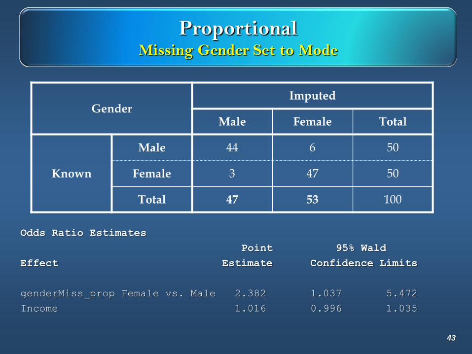
ProportionalMissing Gender Set to Mode
43
GenderImputed
Male Female Total
Known
Male 44 6 50
Female 3 47 50
Total 47 53 100
Odds Ratio Estimates
Point 95% Wald
Effect Estimate Confidence Limits
genderMiss_prop Female vs. Male 2.382 1.037 5.472
Income 1.016 0.996 1.035
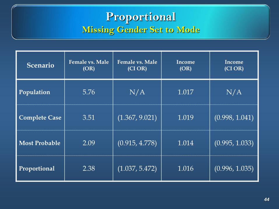
ProportionalMissing Gender Set to Mode
ScenarioFemale vs. Male
(OR)Female vs. Male
(CI OR)Income
(OR)Income (CI OR)
Population 5.76 N/A 1.017 N/A
Complete Case 3.51 (1.367, 9.021) 1.019 (0.998, 1.041)
Most Probable 2.09 (0.915, 4.778) 1.014 (0.995, 1.033)
Proportional 2.38 (1.037, 5.472) 1.016 (0.996, 1.035)
44
Weighted Sequential Hot-Deck ImputationProc HOTDECK in SUDAAN
Weighted Sequential Hot Deck (WSHD)
Imputation:
Weighted: Weights used in selecting donors
Sequential: Order matters in selecting donors
Hot Deck: Uses observe values as donors
Weighted Sequential Hot Deck references - Cox
(1980), Iannacchione (1982), and SUDAAN (2009)
45
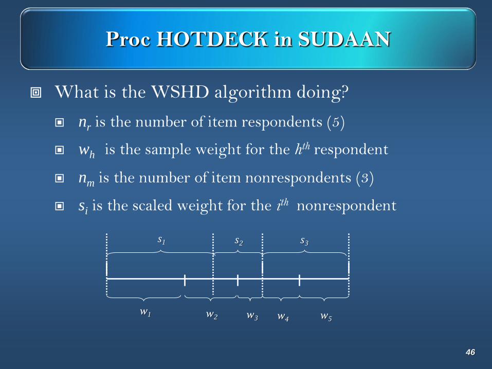
Proc HOTDECK in SUDAAN
What is the WSHD algorithm doing?
nr is the number of item respondents (5)
wh is the sample weight for the hth respondent
nm is the number of item nonrespondents (3)
si is the scaled weight for the ith nonrespondent
46
w1 w
2 w3 w
5w
4
s1 s
2s3
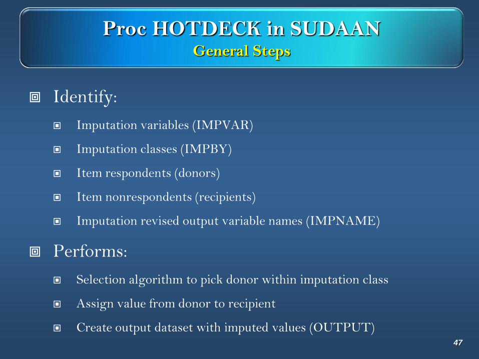
Proc HOTDECK in SUDAANGeneral Steps
Identify:
Imputation variables (IMPVAR)
Imputation classes (IMPBY)
Item respondents (donors)
Item nonrespondents (recipients)
Imputation revised output variable names (IMPNAME)
Performs:
Selection algorithm to pick donor within imputation class
Assign value from donor to recipient
Create output dataset with imputed values (OUTPUT)47
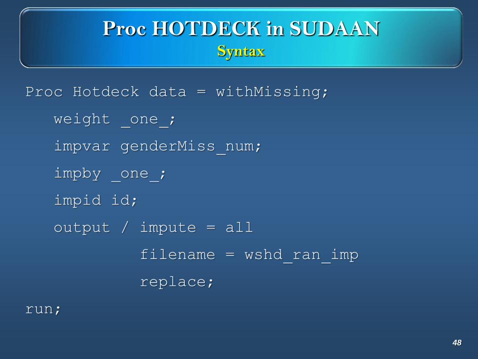
Proc HOTDECK in SUDAANSyntax
Proc Hotdeck data = withMissing;
weight _one_;
impvar genderMiss_num;
impby _one_;
impid id;
output / impute = all
filename = wshd_ran_imp
replace;
run;
48
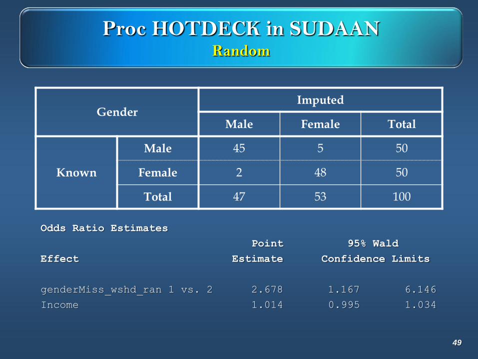
Proc HOTDECK in SUDAANRandom
49
GenderImputed
Male Female Total
Known
Male 45 5 50
Female 2 48 50
Total 47 53 100
Odds Ratio Estimates
Point 95% Wald
Effect Estimate Confidence Limits
genderMiss_wshd_ran 1 vs. 2 2.678 1.167 6.146
Income 1.014 0.995 1.034
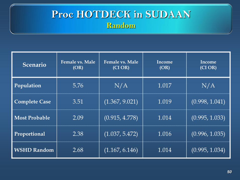
Proc HOTDECK in SUDAANRandom
ScenarioFemale vs. Male
(OR)Female vs. Male
(CI OR)Income
(OR)Income (CI OR)
Population 5.76 N/A 1.017 N/A
Complete Case 3.51 (1.367, 9.021) 1.019 (0.998, 1.041)
Most Probable 2.09 (0.915, 4.778) 1.014 (0.995, 1.033)
Proportional 2.38 (1.037, 5.472) 1.016 (0.996, 1.035)
WSHD Random 2.68 (1.167, 6.146) 1.014 (0.995, 1.034)
50
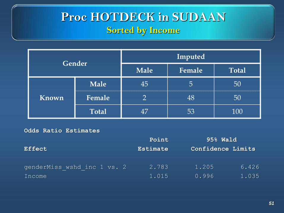
Proc HOTDECK in SUDAANSorted by Income
51
GenderImputed
Male Female Total
Known
Male 45 5 50
Female 2 48 50
Total 47 53 100
Odds Ratio Estimates
Point 95% Wald
Effect Estimate Confidence Limits
genderMiss_wshd_inc 1 vs. 2 2.783 1.205 6.426
Income 1.015 0.996 1.035
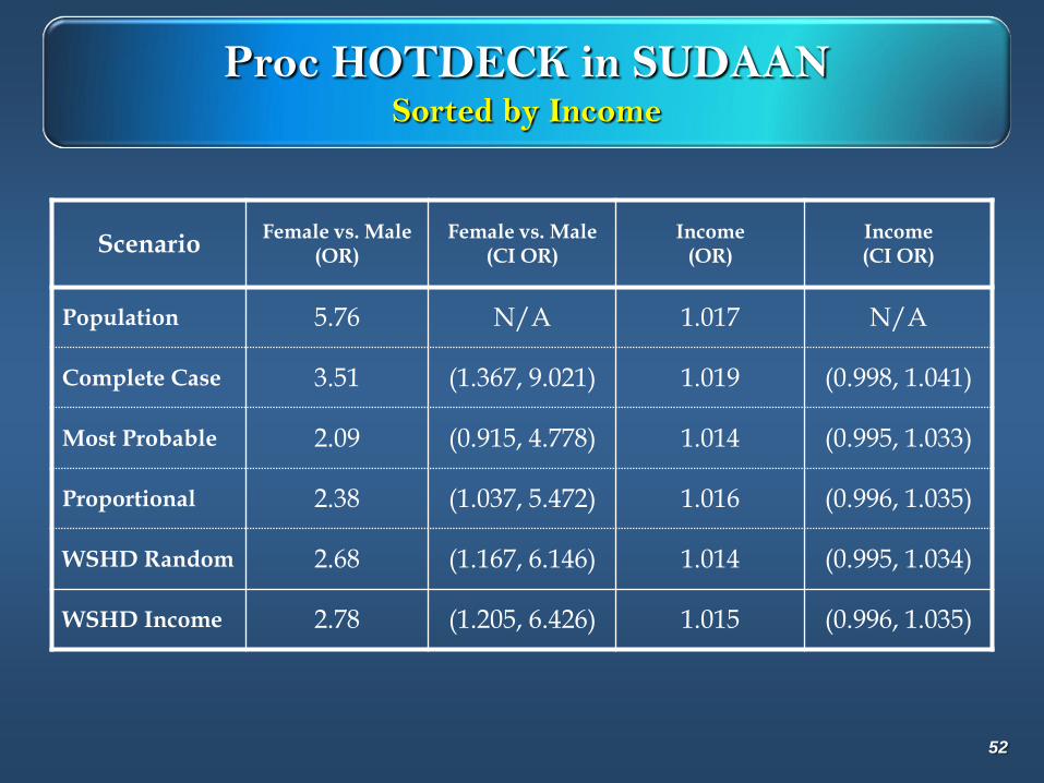
Proc HOTDECK in SUDAANSorted by Income
ScenarioFemale vs. Male
(OR)Female vs. Male
(CI OR)Income
(OR)Income (CI OR)
Population 5.76 N/A 1.017 N/A
Complete Case 3.51 (1.367, 9.021) 1.019 (0.998, 1.041)
Most Probable 2.09 (0.915, 4.778) 1.014 (0.995, 1.033)
Proportional 2.38 (1.037, 5.472) 1.016 (0.996, 1.035)
WSHD Random 2.68 (1.167, 6.146) 1.014 (0.995, 1.034)
WSHD Income 2.78 (1.205, 6.426) 1.015 (0.996, 1.035)
52
Multiple Imputation (MI)
Single imputation may not reflect the uncertainty due to the
imputation but MI can incorporate the imputation
uncertainty in standard errors by:
Repeating the imputation process several times
Estimating the variance inflation from multiple imputations
Why is MI not used more widely?
Lack of knowledge
Lack of software
Lack of infrastructure
Time versus quality
Reference for multiple imputation (Rubin 1987)53
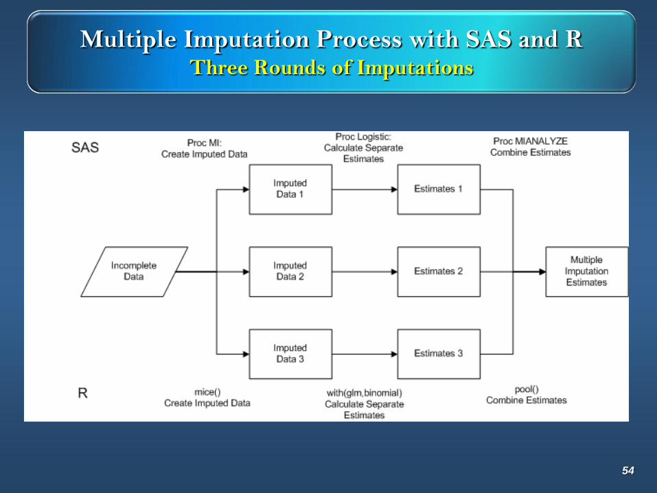
Multiple Imputation Process with SAS and RThree Rounds of Imputations
54
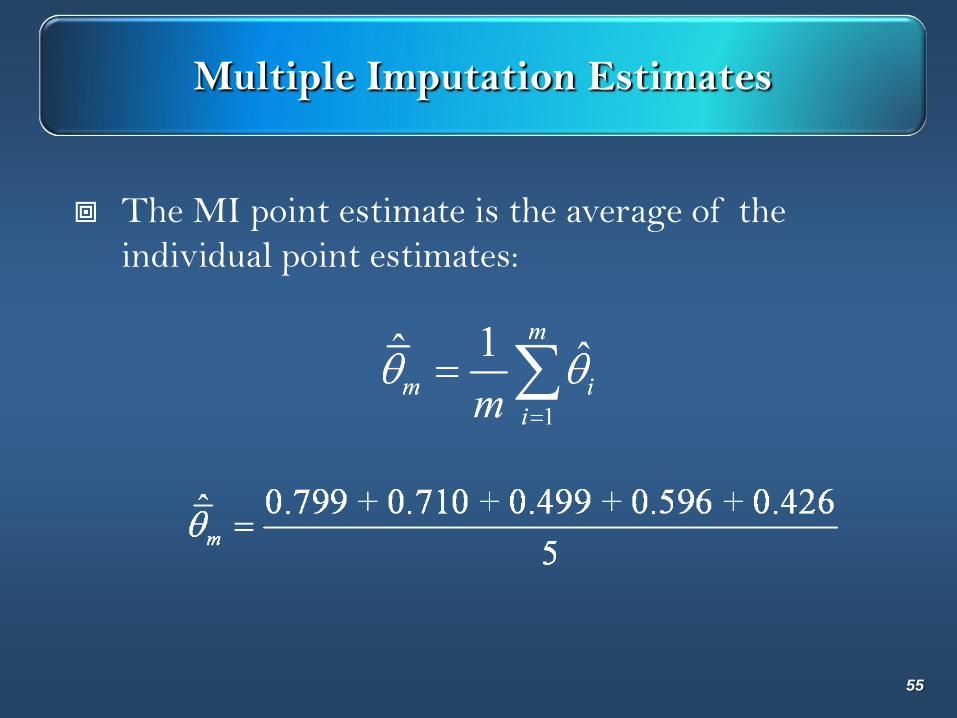
Multiple Imputation Estimates
The MI point estimate is the average of the
individual point estimates:
55
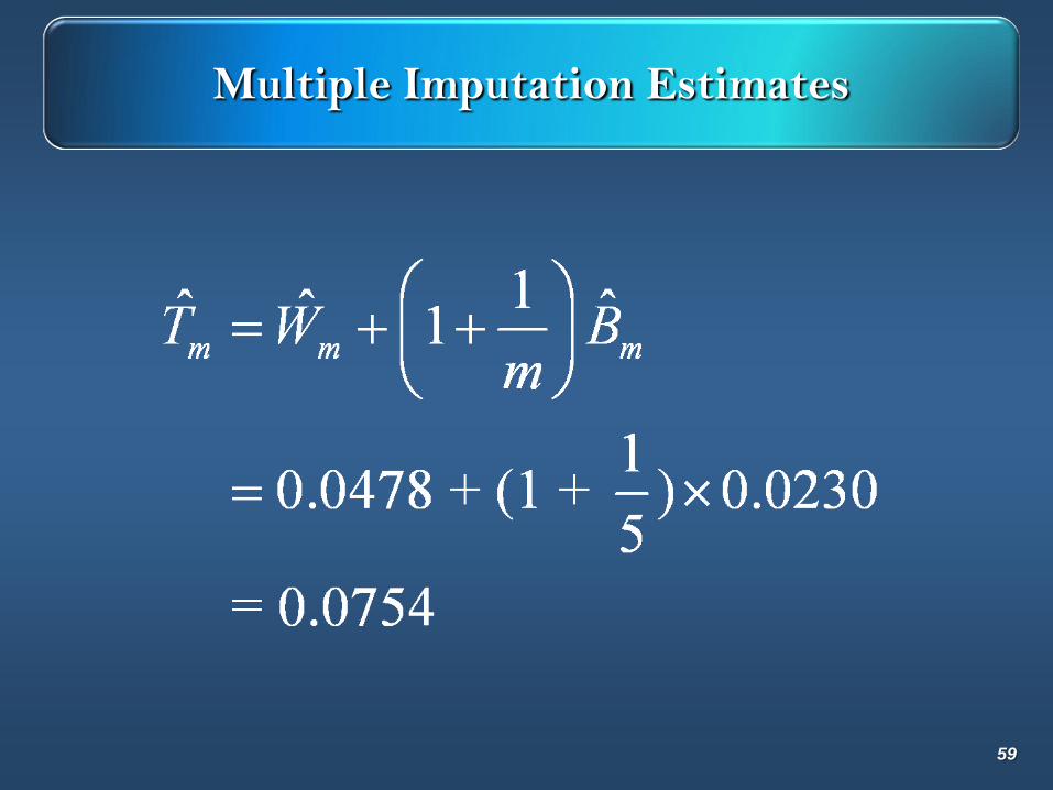
Multiple Imputation Estimates
The MI variance estimate has two components
within and between components:
The within component is the average of the individual
variance estimates from each imputation
The between component is the variance between the
individual point estimates from each imputation
The two components are combined to produce the
total MI variance
56
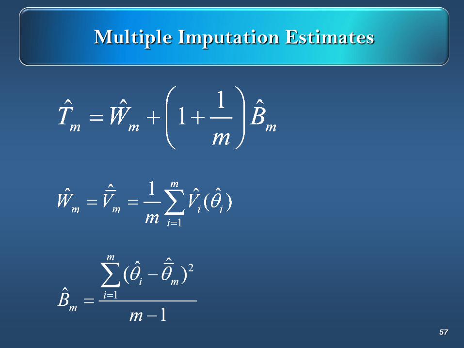
Multiple Imputation Estimates
57
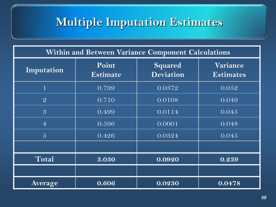
Multiple Imputation Estimates
Within and Between Variance Component Calculations
ImputationPoint
Estimate
Squared
Deviation
Variance
Estimates
1 0.799 0.0372 0.052
2 0.710 0.0108 0.049
3 0.499 0.0114 0.045
4 0.596 0.0001 0.048
5 0.426 0.0324 0.045
Total 3.030 0.0920 0.239
Average 0.606 0.0230 0.0478
58
Multiple Imputation Estimates
59
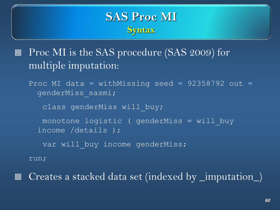
SAS Proc MISyntax
Proc MI is the SAS procedure (SAS 2009) for
multiple imputation:
Proc MI data = withMissing seed = 92358792 out =
genderMiss_sasmi;
class genderMiss will_buy;
monotone logistic ( genderMiss = will_buy
income /details );
var will_buy income genderMiss;
run;
Creates a stacked data set (indexed by _imputation_)
60
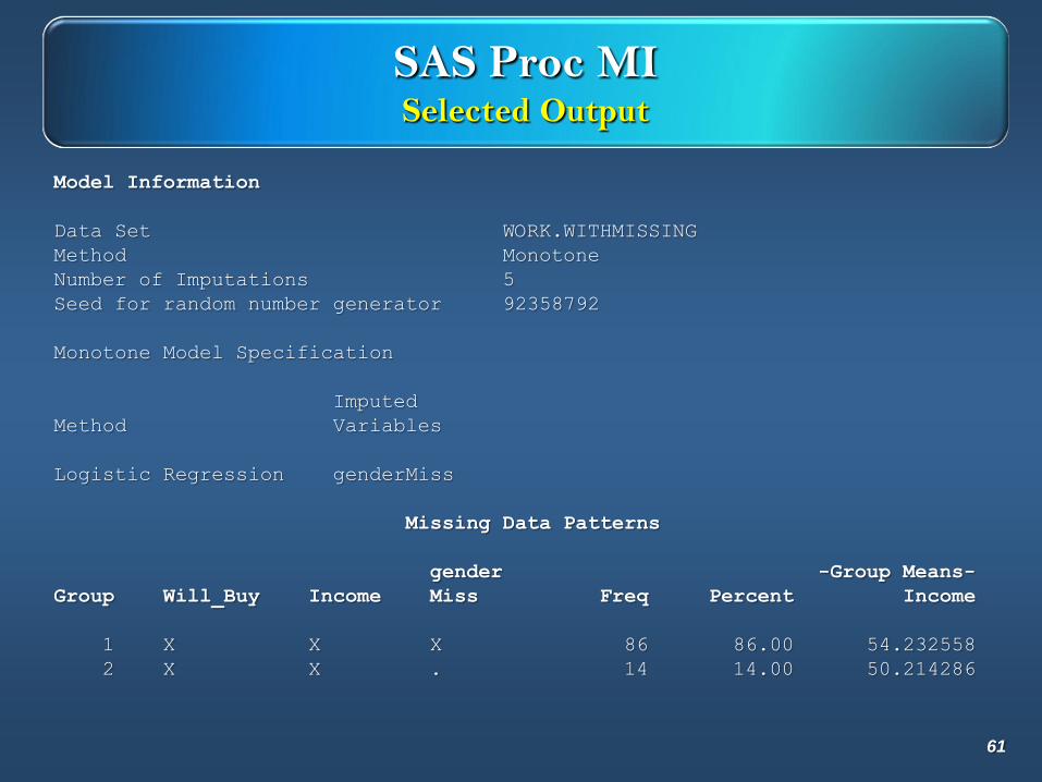
SAS Proc MISelected Output
Model Information
Data Set WORK.WITHMISSING
Method Monotone
Number of Imputations 5
Seed for random number generator 92358792
Monotone Model Specification
Imputed
Method Variables
Logistic Regression genderMiss
Missing Data Patterns
gender -Group Means-
Group Will_Buy Income Miss Freq Percent Income
1 X X X 86 86.00 54.232558
2 X X . 14 14.00 50.214286
61
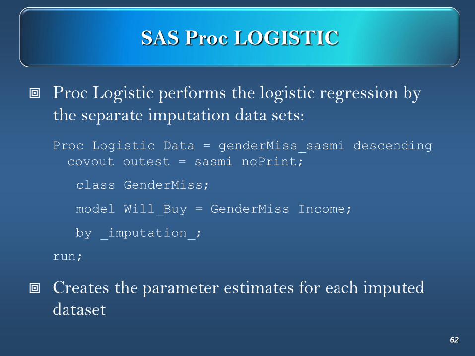
SAS Proc LOGISTIC
Proc Logistic performs the logistic regression by
the separate imputation data sets:
Proc Logistic Data = genderMiss_sasmi descending
covout outest = sasmi noPrint;
class GenderMiss;
model Will_Buy = GenderMiss Income;
by _imputation_;
run;
Creates the parameter estimates for each imputed
dataset
62
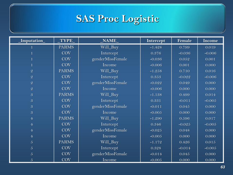
SAS Proc Logistic
_Imputation_ _TYPE_ _NAME_ Intercept Female Income
1 PARMS Will_Buy -1.428 0.799 0.019
1 COV Intercept 0.376 -0.036 -0.006
1 COV genderMissFemale -0.036 0.052 0.001
1 COV Income -0.006 0.001 0.000
2 PARMS Will_Buy -1.258 0.710 0.016
2 COV Intercept 0.353 -0.022 -0.006
2 COV genderMissFemale -0.022 0.049 0.000
2 COV Income -0.006 0.000 0.000
3 PARMS Will_Buy -1.138 0.499 0.014
3 COV Intercept 0.331 -0.011 -0.005
3 COV genderMissFemale -0.011 0.045 0.000
3 COV Income -0.005 0.000 0.000
4 PARMS Will_Buy -1.290 0.596 0.017
4 COV Intercept 0.346 -0.025 -0.005
4 COV genderMissFemale -0.025 0.048 0.000
4 COV Income -0.005 0.000 0.000
5 PARMS Will_Buy -1.172 0.426 0.015
5 COV Intercept 0.328 -0.014 -0.005
5 COV genderMissFemale -0.014 0.045 0.000
5 COV Income -0.005 0.000 0.000
63

SAS Proc MIANALYZESyntax
Proc MIANALYZE combines the information from
different imputations to produce the MI estimates:
Proc mianalyze data = sasmi;
modeleffects intercept gendermissFemale income;
run;
Creates the MI estimates, i.e., the combined
estimates
64
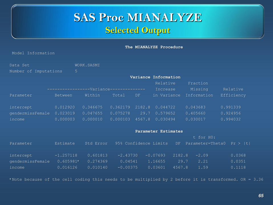
SAS Proc MIANALYZESelected Output
The MIANALYZE Procedure
Model Information
Data Set WORK.SASMI
Number of Imputations 5
Variance Information
Relative Fraction
-----------------Variance-------------- Increase Missing Relative
Parameter Between Within Total DF in Variance Information Efficiency
intercept 0.012920 0.346675 0.362179 2182.8 0.044722 0.043683 0.991339
gendermissFemale 0.023019 0.047655 0.075278 29.7 0.579652 0.405660 0.924956
income 0.000003 0.000010 0.000103 4567.8 0.030494 0.030017 0.994032
Parameter Estimates
t for H0:
Parameter Estimate Std Error 95% Confidence Limits DF Parameter=Theta0 Pr > |t|
intercept -1.257118 0.601813 -2.43730 -0.07693 2182.8 -2.09 0.0368
gendermissFemale 0.605981* 0.274369 0.04541 1.16655 29.7 2.21 0.0351
income 0.016126 0.010140 -0.00375 0.03601 4567.8 1.59 0.1118
*Note because of the cell coding this needs to be multiplied by 2 before it is transformed. OR = 3.36
65
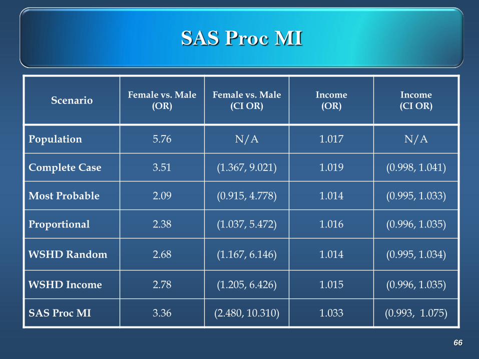
SAS Proc MI
ScenarioFemale vs. Male
(OR)Female vs. Male
(CI OR)Income
(OR)Income(CI OR)
Population 5.76 N/A 1.017 N/A
Complete Case 3.51 (1.367, 9.021) 1.019 (0.998, 1.041)
Most Probable 2.09 (0.915, 4.778) 1.014 (0.995, 1.033)
Proportional 2.38 (1.037, 5.472) 1.016 (0.996, 1.035)
WSHD Random 2.68 (1.167, 6.146) 1.014 (0.995, 1.034)
WSHD Income 2.78 (1.205, 6.426) 1.015 (0.996, 1.035)
SAS Proc MI 3.36 (2.480, 10.310) 1.033 (0.993, 1.075)
66
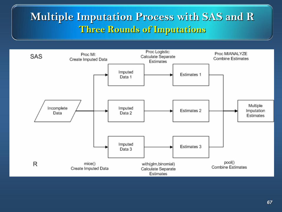
Multiple Imputation Process with SAS and RThree Rounds of Imputations
67
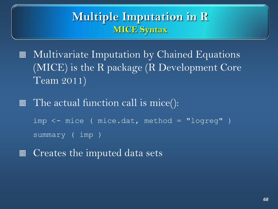
Multiple Imputation in RMICE Syntax
Multivariate Imputation by Chained Equations
(MICE) is the R package (R Development Core
Team 2011)
The actual function call is mice():
imp <- mice ( mice.dat, method = "logreg" )
summary ( imp )
Creates the imputed data sets
68
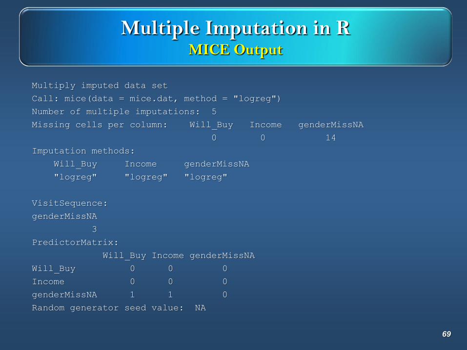
Multiple Imputation in RMICE Output
Multiply imputed data set
Call: mice(data = mice.dat, method = "logreg")
Number of multiple imputations: 5
Missing cells per column: Will_Buy Income genderMissNA
0 0 14
Imputation methods:
Will_Buy Income genderMissNA
"logreg" "logreg" "logreg"
VisitSequence:
genderMissNA
3
PredictorMatrix:
Will_Buy Income genderMissNA
Will_Buy 0 0 0
Income 0 0 0
genderMissNA 1 1 0
Random generator seed value: NA
69

Multiple Imputation in RWITH Syntax
The function call with() evaluates an expression in
multiply imputed data sets. Here the expression is a
logistic regression:
fit <- with ( data = imp, exp = glm ( Will_Buy ~
genderMissNA+Income, family = binomial ))
summary ( fit )
Creates the parameter estimates for each imputation
70
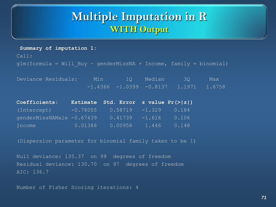
Multiple Imputation in RWITH Output
Summary of imputation 1:
Call:
glm(formula = Will_Buy ~ genderMissNA + Income, family = binomial)
Deviance Residuals: Min 1Q Median 3Q Max
-1.4366 -1.0399 -0.8137 1.1971 1.6758
Coefficients: Estimate Std. Error z value Pr(>|z|)
(Intercept) -0.78055 0.58719 -1.329 0.184
genderMissNAMale -0.67439 0.41739 -1.616 0.106
Income 0.01386 0.00958 1.446 0.148
(Dispersion parameter for binomial family taken to be 1)
Null deviance: 135.37 on 99 degrees of freedom
Residual deviance: 130.70 on 97 degrees of freedom
AIC: 136.7
Number of Fisher Scoring iterations: 4
71
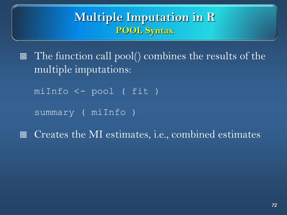
Multiple Imputation in RPOOL Syntax
The function call pool() combines the results of the
multiple imputations:
miInfo <- pool ( fit )
summary ( miInfo )
Creates the MI estimates, i.e., combined estimates
72
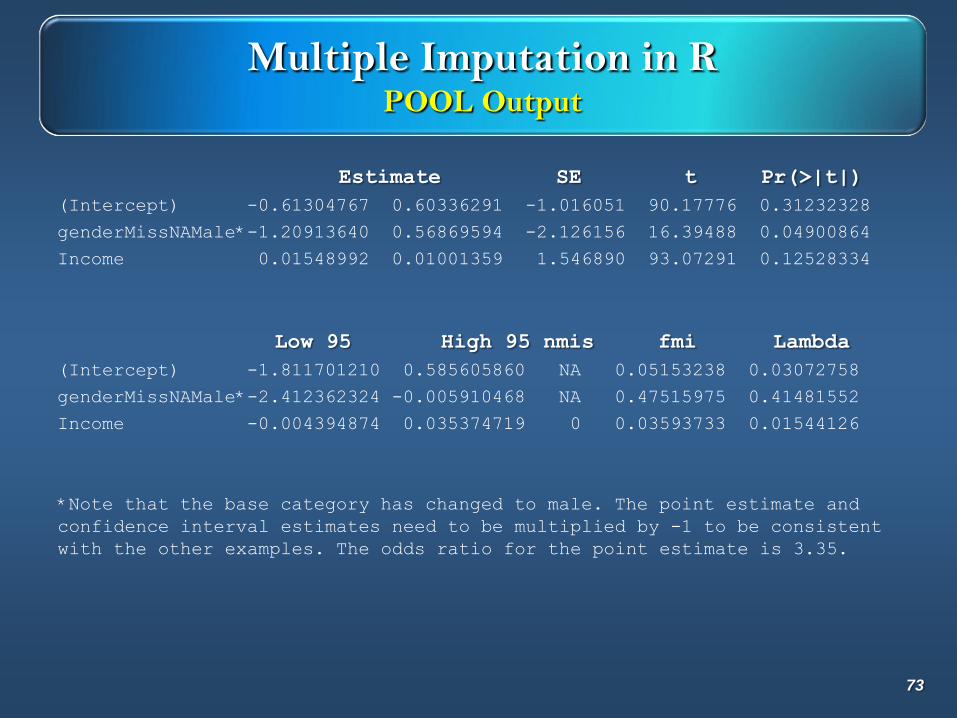
Multiple Imputation in RPOOL Output
Estimate SE t Pr(>|t|)
(Intercept) -0.61304767 0.60336291 -1.016051 90.17776 0.31232328
genderMissNAMale*-1.20913640 0.56869594 -2.126156 16.39488 0.04900864
Income 0.01548992 0.01001359 1.546890 93.07291 0.12528334
Low 95 High 95 nmis fmi Lambda
(Intercept) -1.811701210 0.585605860 NA 0.05153238 0.03072758
genderMissNAMale*-2.412362324 -0.005910468 NA 0.47515975 0.41481552
Income -0.004394874 0.035374719 0 0.03593733 0.01544126
*Note that the base category has changed to male. The point estimate and
confidence interval estimates need to be multiplied by -1 to be consistent
with the other examples. The odds ratio for the point estimate is 3.35.
73
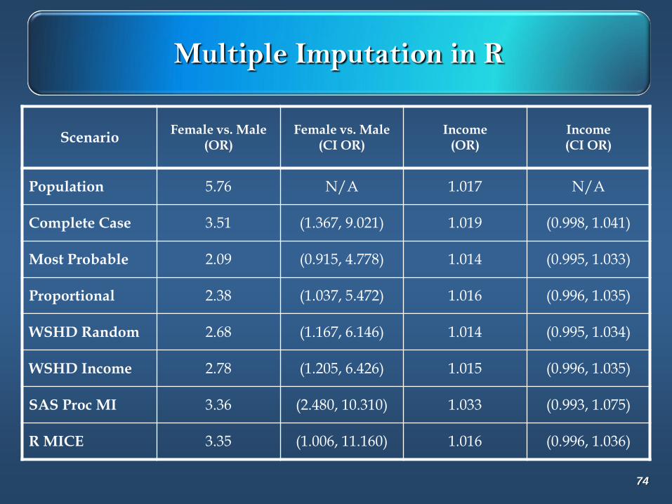
Multiple Imputation in R
ScenarioFemale vs. Male
(OR)Female vs. Male
(CI OR)Income
(OR)Income(CI OR)
Population 5.76 N/A 1.017 N/A
Complete Case 3.51 (1.367, 9.021) 1.019 (0.998, 1.041)
Most Probable 2.09 (0.915, 4.778) 1.014 (0.995, 1.033)
Proportional 2.38 (1.037, 5.472) 1.016 (0.996, 1.035)
WSHD Random 2.68 (1.167, 6.146) 1.014 (0.995, 1.034)
WSHD Income 2.78 (1.205, 6.426) 1.015 (0.996, 1.035)
SAS Proc MI 3.36 (2.480, 10.310) 1.033 (0.993, 1.075)
R MICE 3.35 (1.006, 11.160) 1.016 (0.996, 1.036)
74
Approximate Bayesian Bootstrap (ABB)
Multiple Imputation without explicit distributional
assumptions (Rubin and Schenker 1986)
Respondents: nr
Nonrespondents: nm
Total sample: n = nr + nm
For one round of imputation:
Select a sample WR of size nr from the respondents to create a donor pool
Select a sample WR of size nm as donors
For better results can create classes within which donors are
independently selected75
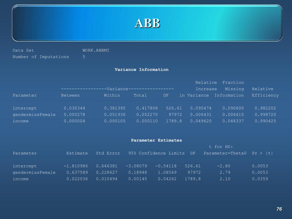
ABB
Data Set WORK.ABBMI
Number of Imputations 5
Variance Information
Relative Fraction
-----------------Variance----------------- Increase Missing Relative
Parameter Between Within Total DF in Variance Information Efficiency
intercept 0.030344 0.381395 0.417808 526.61 0.095474 0.090600 0.982202
gendermissFemale 0.000278 0.051936 0.052270 97972 0.006431 0.006410 0.998720
income 0.000004 0.000105 0.000110 1789.8 0.049620 0.048337 0.990425
Parameter Estimates
t for H0:
Parameter Estimate Std Error 95% Confidence Limits DF Parameter=Theta0 Pr > |t|
intercept -1.810986 0.646381 -3.08079 -0.54118 526.61 -2.80 0.0053
gendermissFemale 0.637589 0.228627 0.18948 1.08569 97972 2.79 0.0053
income 0.022036 0.010494 0.00145 0.04262 1789.8 2.10 0.0359
76
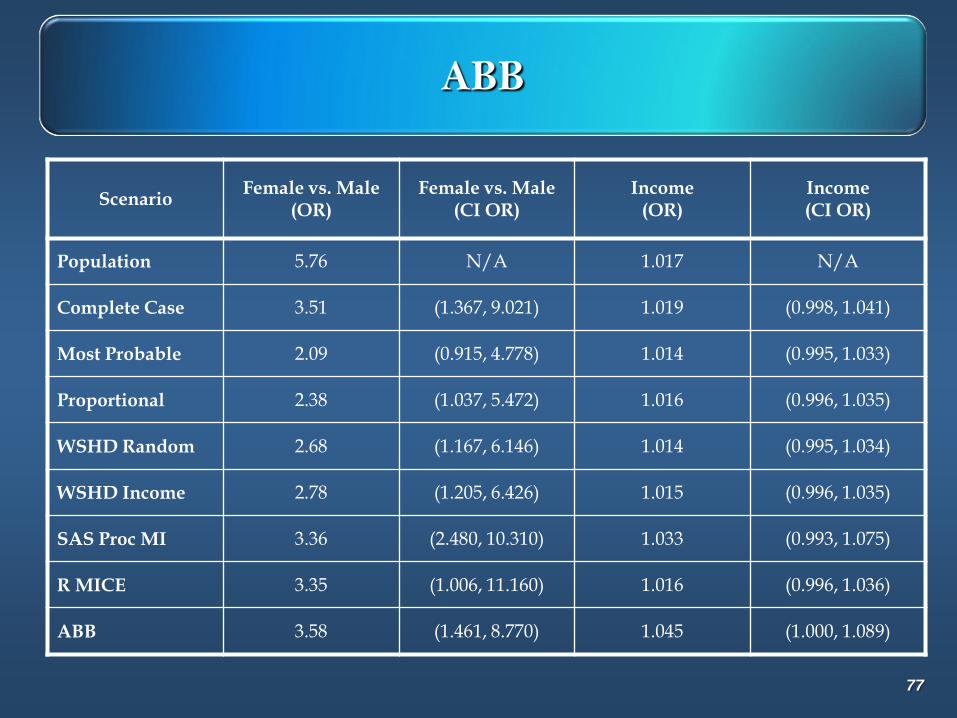
ABB
ScenarioFemale vs. Male
(OR)Female vs. Male
(CI OR)Income
(OR)Income(CI OR)
Population 5.76 N/A 1.017 N/A
Complete Case 3.51 (1.367, 9.021) 1.019 (0.998, 1.041)
Most Probable 2.09 (0.915, 4.778) 1.014 (0.995, 1.033)
Proportional 2.38 (1.037, 5.472) 1.016 (0.996, 1.035)
WSHD Random 2.68 (1.167, 6.146) 1.014 (0.995, 1.034)
WSHD Income 2.78 (1.205, 6.426) 1.015 (0.996, 1.035)
SAS Proc MI 3.36 (2.480, 10.310) 1.033 (0.993, 1.075)
R MICE 3.35 (1.006, 11.160) 1.016 (0.996, 1.036)
ABB 3.58 (1.461, 8.770) 1.045 (1.000, 1.089)
77
Tree, WSHD, and MI
Use the terminal nodes from the tree as imputation
classes, or define them deterministically
Make sure the imputation classes are not too small,
i.e., they have enough donors
Apply WSHD or ABB within the imputation classes
Make sure data set is appropriately configured for
the software to do the analysis
78
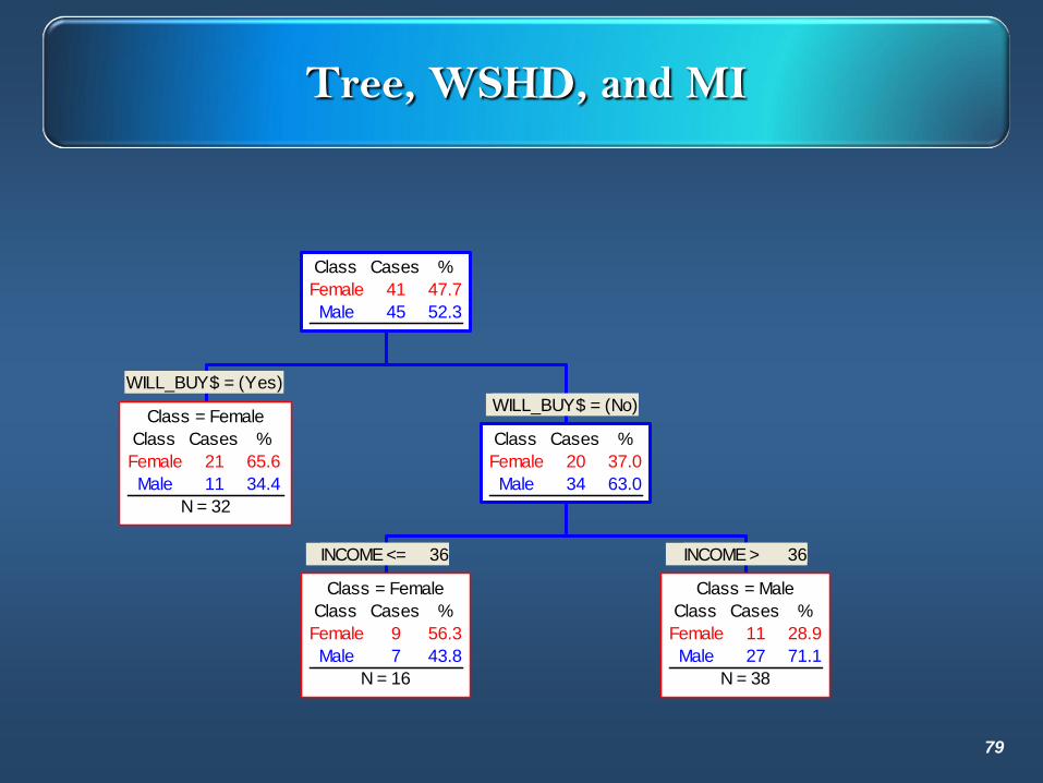
Tree, WSHD, and MI
WILL_BUY$ = (Yes)
Class = Female
Class Cases %
Female 21 65.6
Male 11 34.4
N = 32
INCOME <= 36
Class = Female
Class Cases %
Female 9 56.3
Male 7 43.8
N = 16
INCOME > 36
Class = Male
Class Cases %
Female 11 28.9
Male 27 71.1
N = 38
WILL_BUY$ = (No)
Class Cases %
Female 20 37.0
Male 34 63.0
Class Cases %
Female 41 47.7
Male 45 52.3
79
Tree, WSHD, and MI
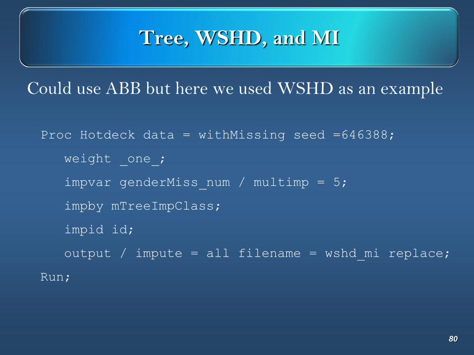
Could use ABB but here we used WSHD as an example
Proc Hotdeck data = withMissing seed =646388;
weight _one_;
impvar genderMiss_num / multimp = 5;
impby mTreeImpClass;
impid id;
output / impute = all filename = wshd_mi replace;
Run;
80
Tree, WSHD, and MI
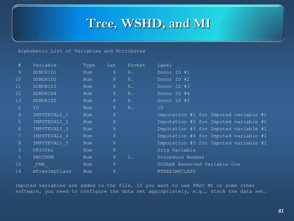
Alphabetic List of Variables and Attributes
# Variable Type Len Format Label
9 DONORID1 Num 8 8. Donor ID #1
10 DONORID2 Num 8 8. Donor ID #2
11 DONORID3 Num 8 8. Donor ID #3
12 DONORID4 Num 8 8. Donor ID #4
13 DONORID5 Num 8 8. Donor ID #5
2 ID Num 8 8. ID
4 IMPUTEVAL1_1 Num 8 Imputation #1 for Imputed variable #1
5 IMPUTEVAL1_2 Num 8 Imputation #2 for Imputed variable #1
6 IMPUTEVAL1_3 Num 8 Imputation #3 for Imputed variable #1
7 IMPUTEVAL1_4 Num 8 Imputation #4 for Imputed variable #1
8 IMPUTEVAL1_5 Num 8 Imputation #5 for Imputed variable #1
3 ORIGVAL Num 8 Orig Variable
1 PROCNUM Num 8 2. Procedure Number
15 _ONE_ Num 8 SUDAAN Reserved Variable One
14 mTreeImpClass Num 8 MTREEIMPCLASS
Imputed variables are added to the file. If you want to use PROC MI or some other
software, you need to configure the data set appropriately, e.g., stack the data set.
81
Tree, WSHD, and MI
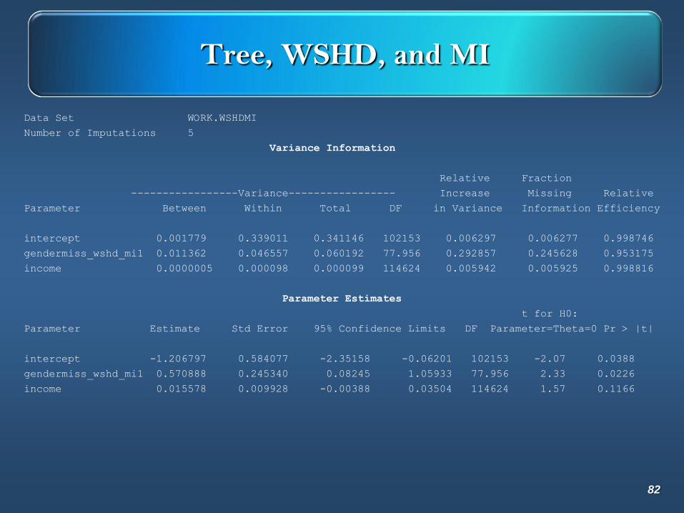
Data Set WORK.WSHDMI
Number of Imputations 5
Variance Information
Relative Fraction
-----------------Variance----------------- Increase Missing Relative
Parameter Between Within Total DF in Variance Information Efficiency
intercept 0.001779 0.339011 0.341146 102153 0.006297 0.006277 0.998746
gendermiss_wshd_mi1 0.011362 0.046557 0.060192 77.956 0.292857 0.245628 0.953175
income 0.0000005 0.000098 0.000099 114624 0.005942 0.005925 0.998816
Parameter Estimates
t for H0:
Parameter Estimate Std Error 95% Confidence Limits DF Parameter=Theta=0 Pr > |t|
intercept -1.206797 0.584077 -2.35158 -0.06201 102153 -2.07 0.0388
gendermiss_wshd_mi1 0.570888 0.245340 0.08245 1.05933 77.956 2.33 0.0226
income 0.015578 0.009928 -0.00388 0.03504 114624 1.57 0.1166
82
Tree, WSHD, and MI
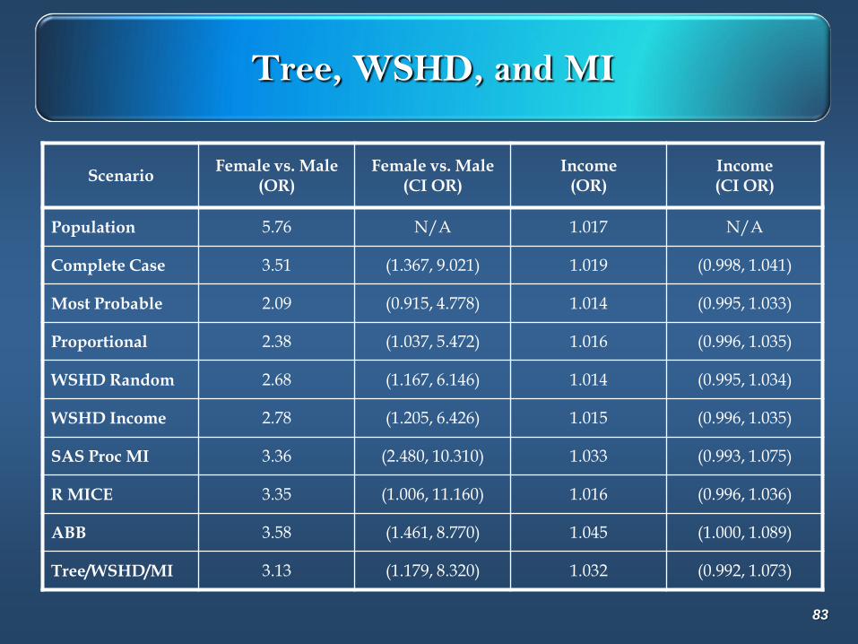
ScenarioFemale vs. Male
(OR)Female vs. Male
(CI OR)Income
(OR)Income(CI OR)
Population 5.76 N/A 1.017 N/A
Complete Case 3.51 (1.367, 9.021) 1.019 (0.998, 1.041)
Most Probable 2.09 (0.915, 4.778) 1.014 (0.995, 1.033)
Proportional 2.38 (1.037, 5.472) 1.016 (0.996, 1.035)
WSHD Random 2.68 (1.167, 6.146) 1.014 (0.995, 1.034)
WSHD Income 2.78 (1.205, 6.426) 1.015 (0.996, 1.035)
SAS Proc MI 3.36 (2.480, 10.310) 1.033 (0.993, 1.075)
R MICE 3.35 (1.006, 11.160) 1.016 (0.996, 1.036)
ABB 3.58 (1.461, 8.770) 1.045 (1.000, 1.089)
Tree/WSHD/MI 3.13 (1.179, 8.320) 1.032 (0.992, 1.073)
83
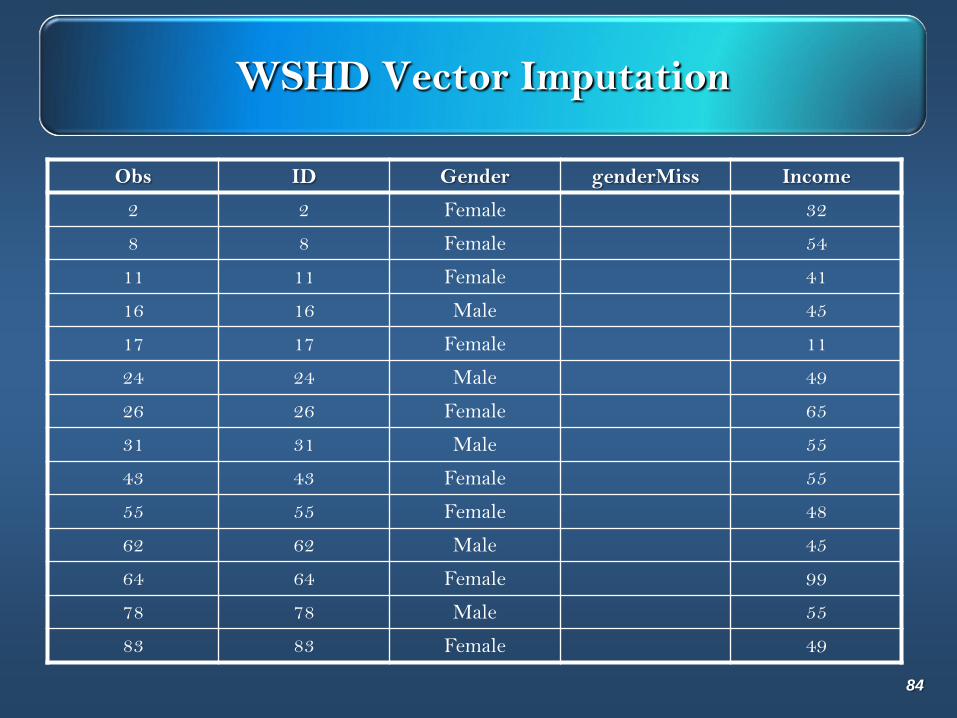
WSHD Vector Imputation
84
Obs ID Gender genderMiss Income
2 2 Female 32
8 8 Female 54
11 11 Female 41
16 16 Male 45
17 17 Female 11
24 24 Male 49
26 26 Female 65
31 31 Male 55
43 43 Female 55
55 55 Female 48
62 62 Male 45
64 64 Female 99
78 78 Male 55
83 83 Female 49
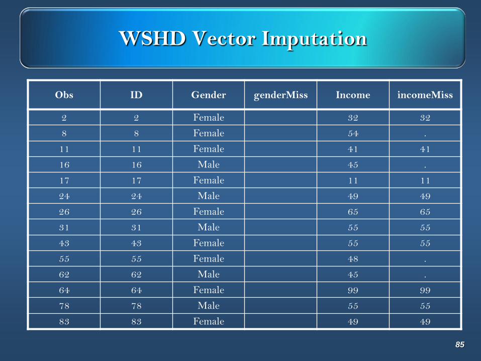
WSHD Vector Imputation
85
Obs ID Gender genderMiss Income incomeMiss
2 2 Female 32 32
8 8 Female 54 .
11 11 Female 41 41
16 16 Male 45 .
17 17 Female 11 11
24 24 Male 49 49
26 26 Female 65 65
31 31 Male 55 55
43 43 Female 55 55
55 55 Female 48 .
62 62 Male 45 .
64 64 Female 99 99
78 78 Male 55 55
83 83 Female 49 49
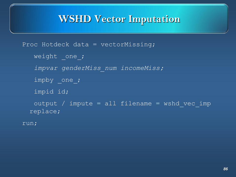
WSHD Vector Imputation
Proc Hotdeck data = vectorMissing;
weight _one_;
impvar genderMiss_num incomeMiss;
impby _one_;
impid id;
output / impute = all filename = wshd_vec_imp
replace;
run;
86
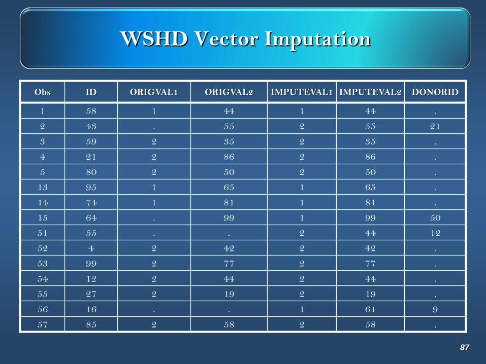
WSHD Vector Imputation
87
Obs ID ORIGVAL1 ORIGVAL2 IMPUTEVAL1 IMPUTEVAL2 DONORID
1 58 1 44 1 44 .
2 43 . 55 2 55 21
3 59 2 35 2 35 .
4 21 2 86 2 86 .
5 80 2 50 2 50 .
13 95 1 65 1 65 .
14 74 1 81 1 81 .
15 64 . 99 1 99 50
51 55 . . 2 44 12
52 4 2 42 2 42 .
53 99 2 77 2 77 .
54 12 2 44 2 44 .
55 27 2 19 2 19 .
56 16 . . 1 61 9
57 85 2 58 2 58 .
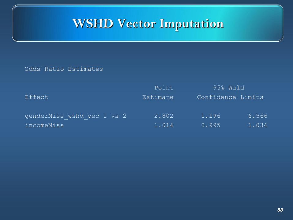
WSHD Vector Imputation
Odds Ratio Estimates
Point 95% Wald
Effect Estimate Confidence Limits
genderMiss_wshd_vec 1 vs 2 2.802 1.196 6.566
incomeMiss 1.014 0.995 1.034
88
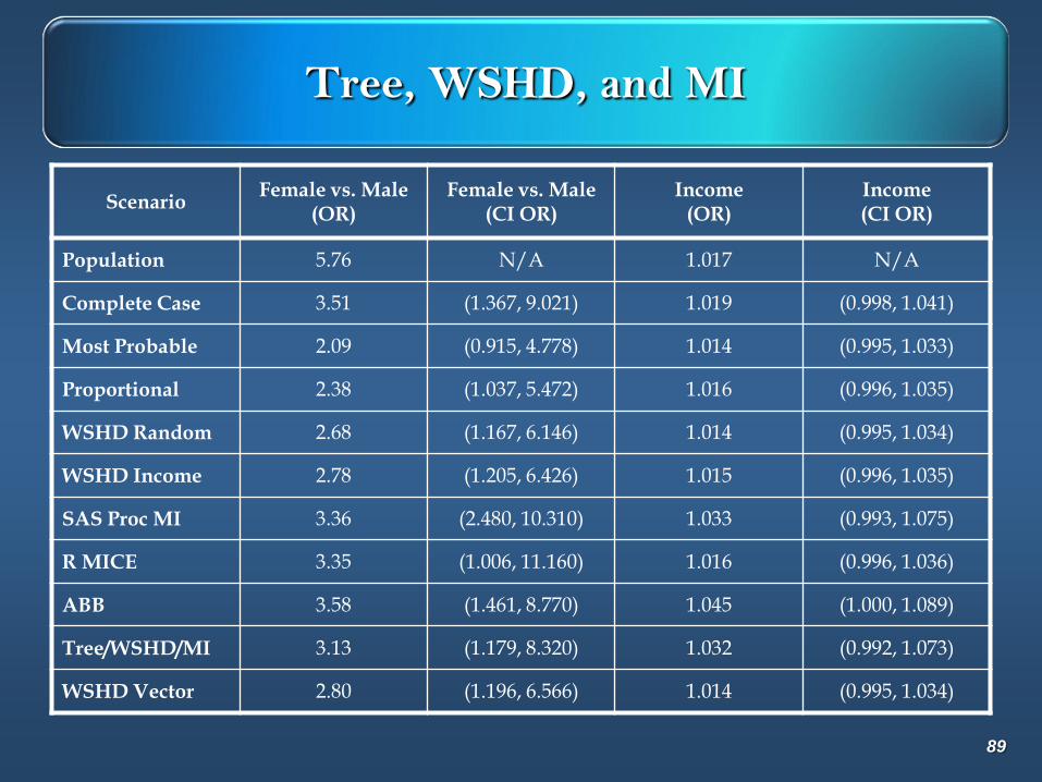
Tree, WSHD, and MI
ScenarioFemale vs. Male
(OR)Female vs. Male
(CI OR)Income
(OR)Income(CI OR)
Population 5.76 N/A 1.017 N/A
Complete Case 3.51 (1.367, 9.021) 1.019 (0.998, 1.041)
Most Probable 2.09 (0.915, 4.778) 1.014 (0.995, 1.033)
Proportional 2.38 (1.037, 5.472) 1.016 (0.996, 1.035)
WSHD Random 2.68 (1.167, 6.146) 1.014 (0.995, 1.034)
WSHD Income 2.78 (1.205, 6.426) 1.015 (0.996, 1.035)
SAS Proc MI 3.36 (2.480, 10.310) 1.033 (0.993, 1.075)
R MICE 3.35 (1.006, 11.160) 1.016 (0.996, 1.036)
ABB 3.58 (1.461, 8.770) 1.045 (1.000, 1.089)
Tree/WSHD/MI 3.13 (1.179, 8.320) 1.032 (0.992, 1.073)
WSHD Vector 2.80 (1.196, 6.566) 1.014 (0.995, 1.034)
89
Imputation Diagnostics
90

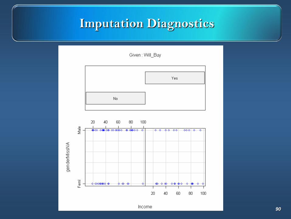
Imputation DiagnosticsConditional Plot
91

Imputation DiagnosticsMosaic Plot
92
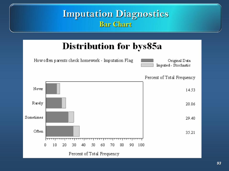
Imputation DiagnosticsBar Chart
93
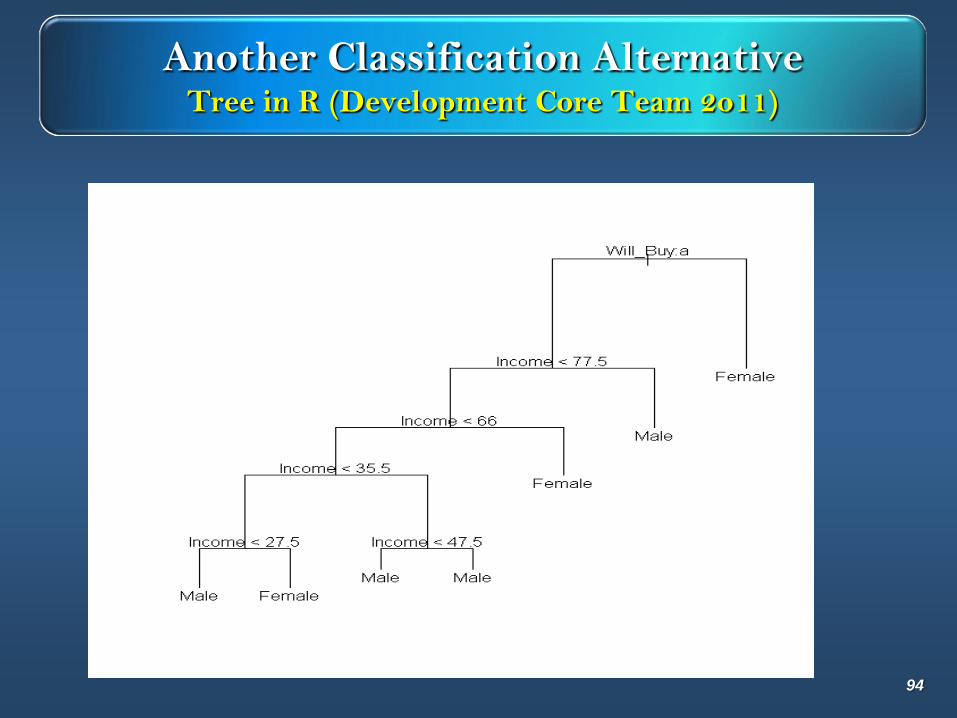
Another Classification AlternativeTree in R (Development Core Team 2o11)
94
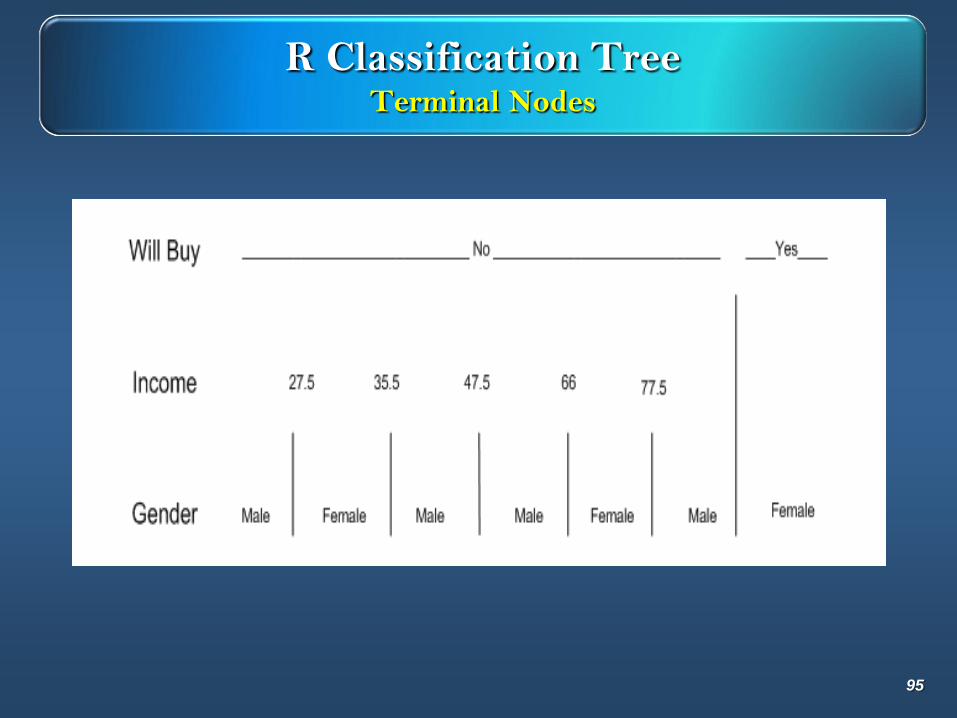
R Classification TreeTerminal Nodes
95
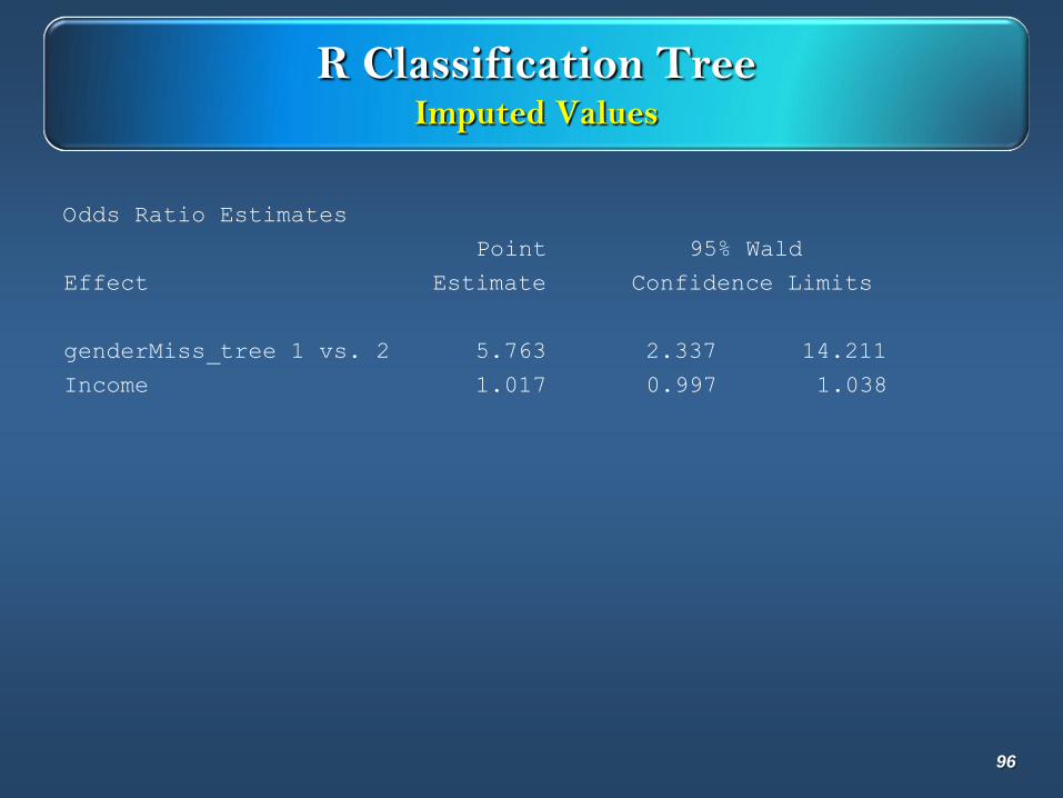
R Classification TreeImputed Values
Odds Ratio Estimates
Point 95% Wald
Effect Estimate Confidence Limits
genderMiss_tree 1 vs. 2 5.763 2.337 14.211
Income 1.017 0.997 1.038
96
Multiple Imputation with IVEware
IVEware (Raghuhatan et alia 2002) is a suite of SAS macros for conducting multiple imputation
Two-step process
Impute
Creates a stacked data set (indexed by _mult_)
Need to create separate data sets from the stacked data set
Analyze
Creates individual estimates
Combines individual estimates to create MI estimate
97
Multiple Imputation with IVEwareSyntax
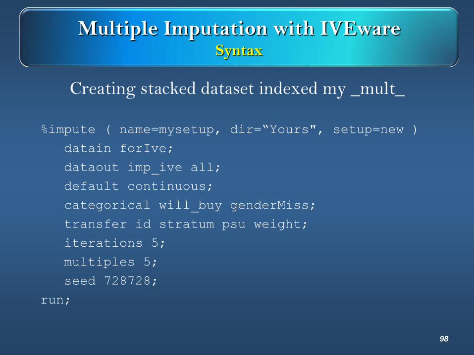
Creating stacked dataset indexed my _mult_
%impute ( name=mysetup, dir=“Yours", setup=new )
datain forIve;
dataout imp_ive all;
default continuous;
categorical will_buy genderMiss;
transfer id stratum psu weight;
iterations 5;
multiples 5;
seed 728728;
run;
98
Multiple Imputation with IVEwareAnalyze
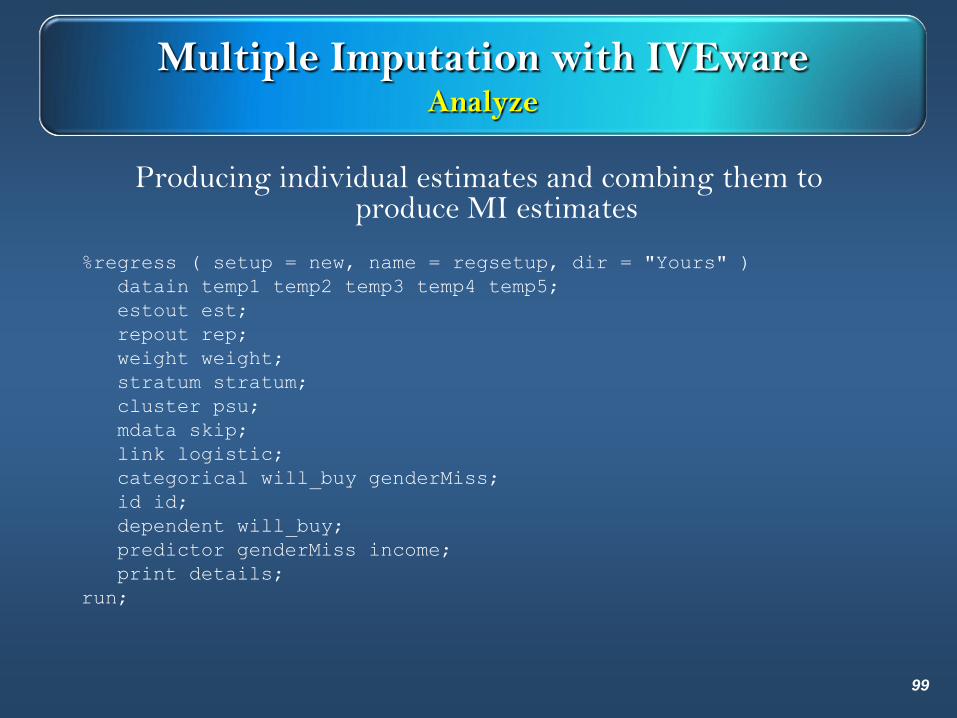
Producing individual estimates and combing them to produce MI estimates
%regress ( setup = new, name = regsetup, dir = "Yours" )
datain temp1 temp2 temp3 temp4 temp5;
estout est;
repout rep;
weight weight;
stratum stratum;
cluster psu;
mdata skip;
link logistic;
categorical will_buy genderMiss;
id id;
dependent will_buy;
predictor genderMiss income;
print details;
run;
99
Multiple Imputation with IVEwareEstimation
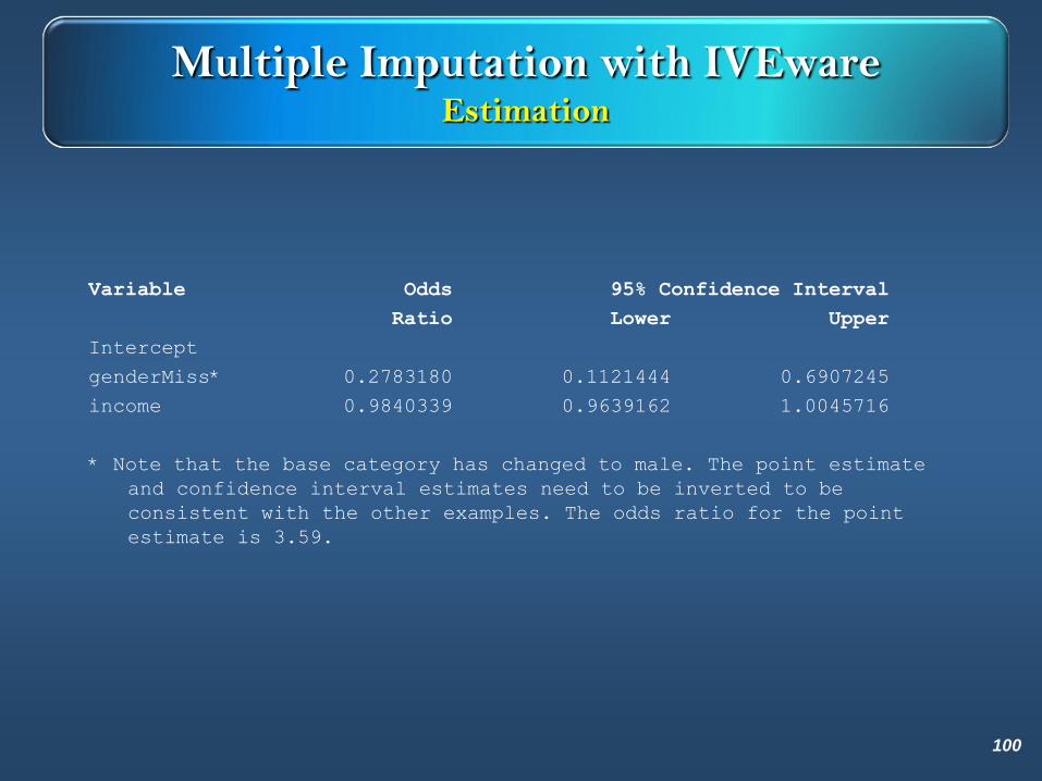
Variable Odds 95% Confidence Interval
Ratio Lower Upper
Intercept
genderMiss* 0.2783180 0.1121444 0.6907245
income 0.9840339 0.9639162 1.0045716
* Note that the base category has changed to male. The point estimate
and confidence interval estimates need to be inverted to be
consistent with the other examples. The odds ratio for the point
estimate is 3.59.
100

Multiple Imputation with IVEware
ScenarioFemale vs. Male
(OR)Female vs. Male
(CI OR)Income
(OR)Income(CI OR)
Population 5.76 N/A 1.017 N/A
Complete Case 3.51 (1.367, 9.021) 1.019 (0.998, 1.041)
Most Probable 2.09 (0.915, 4.778) 1.014 (0.995, 1.033)
Proportional 2.38 (1.037, 5.472) 1.016 (0.996, 1.035)
WSHD Random 2.68 (1.167, 6.146) 1.014 (0.995, 1.034)
WSHD Income 2.78 (1.205, 6.426) 1.015 (0.996, 1.035)
SAS Proc MI 3.36 (2.480, 10.310) 1.033 (0.993, 1.075)
R MICE 3.35 (1.006, 11.160) 1.016 (0.996, 1.036)
IVEware 3.59 (1.448, 8.917) 1.016 (0.995, 1.037)
101