mixing in water supply service tanks and...
TRANSCRIPT

MIXING IN WATER
SUPPLY SERVICE TANKS
AND RESERVOIRS
Preethi Shivaram
Supervisor:
Prof. Greg Ivey
November 2007


Faculty of Engineering
The University of Western Australia
35 Stirling HWY
Crawley WA 6009
Attention: The Dean
Dear Sir,
It is with great pleasure that I submit this thesis, entitled “Mixing in Water Supply Tanks and
Reservoirs”, as a partial fulfilment of the requirements for the degree of Bachelor of Engineering
(Environmental) with Honours.
Yours Sincerely,
Preethi Shivaram


Abstract
This project investigates the internal mixing process caused by turbulent jet inflows in drinking water
supply tanks and reservoirs. In these service tanks and reservoirs, complete mixing is essential to
ensure both an even distribution of disinfectants and to minimise the decay of the disinfectants when
trapped in older unmixed pockets of water. Of particular importance to tank operation and design, is
the determination of the time required for a tank to be completely mixed. The existing literature on
mixing time and fluid behaviour within confined systems is limited and fragmented. Numerous mixing
time formulae exist, which from the outset are derived by various means. The aim of the present study
is to derive a mixing time formula that can be used in the design, operation and analysis of water
distribution tanks and reservoirs, during neutrally buoyant situations. The project is undertaken by the
systematic consolidation and critical analysis of: the fundamentals of jet flow, existing formulae,
historical data, and numerical data. The numerical data is derived from CFD modelling using the
program, CFX. In doing so, the project also consolidates and analyses the experimental measurement
techniques for jet mixing. This detailed approach to confined jet mixing with the focus of deriving a
mixing time formula, has not been undertaken in previous studies. Hence, the present work is of
crucial benefit to the water industry, specifically those involved in tank design and analysis.
It was found that existing formulae have been derived from limited testing on the effects of tank aspect
ratios on jet mixing. Thus, CFD modelling was used to generate a data set that spans a larger set of
aspect ratios to previous studies, to ensure the robustness of the proposed mixing time formula over a
wider range of tank geometries. The dimensionless mixing time formula is found to be, 9.03.2
5.7 ⎟⎠⎞
⎜⎝⎛
⎟⎟⎠
⎞⎜⎜⎝
⎛=
DH
dDT
nm
. The effect of inlet configuration is also investigated and the common practise
of attempting to capture this effect via the free jet path length parameter is disproved with
experimental evidence. The experimental methods employed to measure mixing time are also
investigated. It is found that CFD modelling and the LIF method of physical scale modelling for tank
mixing have the potential to overestimate of mixing time. The overestimation of mixing time can
introduce significant, unnecessary costs to the construction and retrofitting of water supply tanks. This
finding has not been reported in previous studies.
I

Acknowledgements
I would like to take this opportunity to acknowledge a number of people for their help and
support during the progress of this project.
Most importantly I would like to first extend a special thank you to my supervisors Prof.
Greg Ivey his guidance and support during all stages of the project. I would also like to extend another
special thank you to Thomas Ewing, from GHD, for his help, patience and time in the Computational
Fluid Dynamic Modelling stage of the project. I would also like to thank Jose Romareo and David
Horn, from GHD, for the development and initial help in learning about the project.
I would like to thank my family and friends for the wonderful support and enthusiasm provided during
the time of this project.
II
Table of Contents
1 NOTATION: ......................................................................................................... 1
2 INTRODUCTION ................................................................................................. 3
3 LITERATURE REVIEW ....................................................................................... 7
3.1 Free jet theory .......................................................................................................................................... 7 3.1.1 Jet formation.......................................................................................................................................... 7 3.1.2 Jet parameters ........................................................................................................................................ 7 3.1.3 Regions.................................................................................................................................................. 8 3.1.4 Entrainment ........................................................................................................................................... 9
3.2 Confined jet ............................................................................................................................................ 12 3.2.1 Mixing time for negligible boundary interaction cases ....................................................................... 12 3.2.2 Mixing time for significant boundary interaction cases....................................................................... 13
3.3 Formulae from previous studies ........................................................................................................... 16 3.3.1 Theory based formulae ........................................................................................................................ 17 3.3.2 Other formulae..................................................................................................................................... 27 3.3.3 Generalised mixing time formula ........................................................................................................ 29
3.4 Tank operation mode............................................................................................................................. 44
3.5 Experimental Method Evaluation ........................................................................................................ 45 3.5.1 Definition of mixing time .................................................................................................................... 45 3.5.2 Probe measurement.............................................................................................................................. 46
3.6 Existing Guidelines ................................................................................................................................ 47
3.7 Supporting Experimental Works ......................................................................................................... 48
4 METHODOLOGY .............................................................................................. 49
4.1 Review of historical results and data.................................................................................................... 49 4.1.1 Limitations........................................................................................................................................... 50
4.2 CFD modelling ....................................................................................................................................... 51 4.2.1 Overview ............................................................................................................................................. 51 4.2.2 Validation of numerical results............................................................................................................ 52 4.2.3 Model specification ............................................................................................................................. 56
III
4.2.4 Simulation details ................................................................................................................................ 59 4.2.5 Limitations........................................................................................................................................... 61
5 RESULTS .......................................................................................................... 65
5.1 Parameter ranges investigated in previous studies ............................................................................. 65 5.1.1 Tank to nozzle diameter ration (D/dn)................................................................................................. 65 5.1.2 Tank height to diameter ratio............................................................................................................... 69
5.2 CFD Modelling....................................................................................................................................... 71
5.3 Constant, β.............................................................................................................................................. 74
6 DISCUSSION..................................................................................................... 77
6.1 Tank and nozzle diameter ratio (D/dn)................................................................................................ 77 6.1.1 Summary ............................................................................................................................................. 79
6.2 Tank height to diameter ratio (H/D) .................................................................................................... 80 6.2.1 Historical results and data.................................................................................................................... 80 6.2.2 CFD modelling .................................................................................................................................... 81 6.2.3 Summary ............................................................................................................................................. 82
6.3 Constant, β.............................................................................................................................................. 82
6.4 Summary................................................................................................................................................. 83
7 CONCLUSIONS ................................................................................................ 85
8 RECOMMENDATIONS FOR FURTHER RESEARCH...................................... 89
9 REFERENCES .................................................................................................. 91
10 APPENDIX ..................................................................................................... 93
10.1 CFD Validation Data Experimental Setup .......................................................................................... 93
10.2 Calculation of the free jet length (L) .................................................................................................... 94
10.3 Meshing details....................................................................................................................................... 95
IV

List of Figures Figure 3.1.1 Jet Flow Dynamics (Revill, 1992) ...................................................................................... 8 Figure 3.1.2 Experimental evidence of linear jet dilution relationship (Fisher et al., 1979). ................ 10 Figure 3.2.1 Velocity vector profiles indicating angled entrainment for jet mixers (Zughbi and Rakib,
2004)...................................................................................................................................................... 15 Figure 3.3.1 Damping oscillation response curve due to circulatory flows (Maruyama et al., 1982)... 21 Figure 3.3.2 Definition of free jet path length (Maruyama et al., 1982). .............................................. 22 Figure 3.3.3 Circulation patterns induced for: (a) circular jet and (b) wall jet (Maruyama et al., 1982).
............................................................................................................................................................... 23 Figure 3.3.4 Definition of free jet path length, L, for (a) centre, bottom, vertical feed inlet, and (b) side,
bottom, vertical feed inlet...................................................................................................................... 32 Figure 3.3.5 Measurement of jet angle.................................................................................................. 33 Figure 3.3.6 Influence of nozzle angle and diameter on mixing time (Dakshinamoorthy et al., 2006).33 Figure 3.3.7 CFD modelling mixing time results for various nozzle angles by Zughbi and Rakib
(2004). ................................................................................................................................................... 34
Figure 3.3.8 Velocity profiles at nozzle angles of (a) 60° and (b) 30° (Zughbi and Rakib, 2004). ...... 35 Figure 3.3.9 Mixing time results for various nozzle angles (Patwardhan and Gaikwad, 2003)............ 35
Figure 3.3.10 Velocity profiles for nozzle angles of (a) 45° and (b) 30° (Zughbi and Rakib, 2004).... 37
Figure 3.3.11 Velocity profiles for nozzle angles of (a) 20° and (b) 30° (Zughbi and Rakib, 2004).... 38 Figure 3.3.12 Mixing time results from various nozzle locations (Zughbi and Rakib, 2004)............... 39 Figure 3.3.13 Velocity profiles for nozzle locations at (a) hi/H=0.2, (b) hi/H=0.3, (c) hi/H=0.5......... 40 Figure 3.3.14 Dimensionless mixing times (Tm=untm/dn) for a side, vertical feed inlet (GCO1) and
centre, vertical feed inlet (GC02) (Roberts et al., 2006). ...................................................................... 41 Figure 3.3.15 Donut shaped dead zones for centre, vertical feed inlets (Roberts et al., 2006) ............. 42 Figure 3.3.16 Effect of inflow rate on the size of dead zones (Roberts et al., 2006). ........................... 42 Figure 3.4.1 Experimental details of investigations into the effect of tank operation mode on mixing
time (Roberts et al., 2006). .................................................................................................................... 44 Figure 3.5.1 Chart recorder plot of a conductivity trace after addition of a tracer (Lane and Rice,
1982)...................................................................................................................................................... 46 Figure 4.2.1 Tracer concentration profiles produced by Roberts et al. (2006) for a mixed tank. ......... 54 Figure 4.2.2 Tracer concentration plot for validation simulation produced by numerical model. ........ 55 Figure 4.2.3 Tracer concentration profiles at the end of the mixing period for inflow velocities of 8 and
7 ft/s, respectively (Roberts et al., 2005)............................................................................................... 56 Figure 4.2.4 Illustration of the type of tank geometry used in the numerical modelling process. ........ 57 Figure 4.2.5 Determination of mixing time for the numerical output of simulation 3 during CFD
modelling............................................................................................................................................... 60
V
Figure 4.2.6 Snapshot of the evaluation plane for tanks with different H/D ratios, where H/D for case
(a) is less than H/D for case (b). ............................................................................................................ 62 Figure 5.1.1 Parameterisation of (D/dn) from historical data using various H/D values. .................... 65 Figure 5.1.2 5.1.3 Parameterisation of (D/dn) from historical data for H/D=0.5................................. 66 Figure 5.1.4 Parameterisation of (D/dn) from historical data- were H/D =1.0 ................................... 67 Figure 5.1.5 Parameterisation of the H/D ratio using historical data only. ........................................... 69 Figure 5.1.6 Parameterisation of (H/D) with respect to the range of aspect ratios testing. ................... 70 Figure 5.2.1 Parameterisation of H/D using numerical and historical data, over various D/dn ratios. . 72 Figure 5.2.2 Parameterisation of H/D ratio from collating numerical and historical data for D/dn=100.
............................................................................................................................................................... 73 Figure 5.2.3 Parameterisation of H/D ratio by collating all historical and numerical data for D/dn=100,
150 and 200. .......................................................................................................................................... 74 Figure 5.3.1 Evaluation of the constant using only the results of the numerical study. ........................ 75 Figure 5.3.2 Evaluation of the constant using numerical and historical results for a D/dn=100........... 75 Figure 5.3.3 Evaluation of the constant using numerical and historical results for a D/dn=100, 150 and
200......................................................................................................................................................... 76 Figure 6.1.1 Experimental Set-up of Patwardhan (2002)...................................................................... 79 Figure 6.1.2 Normalised concentration profiles at each probe from physical scale modelling
experiments performed by Patwardhan (2002). .................................................................................... 79 Figure 10.1.1 Experimental Setup of Roberts et al. (2006)................................................................... 93 Figure 10.2.1 Side view of tank ............................................................................................................ 94 Figure 10.3.1 Side view of the plane of symmetry for the grid used in CFD modelling stage ............ 95 Figure 10.3.2 View of tank centred on z-axis used in CFD modelling stage....................................... 95
VI

VII
List of Tables
Table 3.3.1 Mixing time formulae presented by previous studies......................................................... 17 Table 3.3.2 Mixing time formula proposed by different authors presented in a common form, where
(Tm=untm/dn)........................................................................................................................................... 30 Table 4.2.1 Summary simulation details performed via CFD modelling.............................................. 59 Table 4.2.2 Details of each individual simulation conducted................................................................ 59 Table 5.1.1 Summary details for regressions performed in Figure 5.1.1. ............................................. 66 Table 5.1.2 Summary of parameterisation regressions performed in Figure 5.1.1 to Figure 5.1.4. ...... 68 Table 5.1.3 Summary details for regressions performed in Figure 5.1.6. ............................................. 70 Table 6.1.1 Comparison of the value of the constant in the mixing time formula, derived by various
studies.................................................................................................................................................... 83

Notation
1
1 Notation:
a parameterisation constant for D/dn ratio
A cross-sectional area of jet, m2
b parameterisation constant for H/D ratio
Ct tracer concentration, gm-3
Ct0 initial tracer concentration, gm-3
tc mean tracer concentration of fully mixed system, gm-3
dn nozzle diameter, m
D tank diameter, m
Fr Froude number, (Fr=un/(gH)1/2)
g gravitational acceleration, ms-2
hi height of nozzle from base of tank, m
H liquid height in tank prior to jet injection, m
L free jet path length, m
Ql characteristic length scale of a pure jet, m
Mn initial jet momentum flux, m4s-2
QL flow rate at end of free jet path length, L, from inlet, m3s-1
Qn initial flow rate, m3s-1
Ren jet Reynolds number, (Ren =undn/ν)
t time elapsed after jet injection, s
tm mixing time, s
tc mean circulation time, s
Tm dimensionless mixing time, (Tm= tmun/dn)
uz time-averaged jet velocity in the axial direction, ms-1
um maximum centreline velocity, ms-1
un jet velocity at nozzle, ms-1
Vt tank volume, m3
z axial direction of jet, m
Greek symbols
β constant
θ nozzle angle from horizontal, degrees
ε dissipation rate, m2s-3

Notation
2
κ turbulent kinetic energy, m2s-2
μ flow rate at some axial distance from inlet, m3s-1
ν kinematic viscosity, m2s-1
γ angle of jet spread from the axial direction of jet flow, degrees

Introduction
3
2 Introduction
Storage facilities are essential features of water distributions systems and have the function of:
providing emergency storage, equalising pressure and balancing water usage during the day.
Traditionally, tank design only catered for these functions. The identification that water quality within
the tanks also needs to be considered in tank design is a relatively recent phenomenon. For this reason
the mixing processes within drinking water storage facilities has only been studied formally in recent
years.
Many water distribution storage tanks use a jet mixing process to mix the inflow water with the
ambient tank water. The jet is produced by the inflow of water into a water body. Mixing is any
process which causes one parcel of water to me mingled with or diluted by another (Fischer et al.
1979). The jet mixing process within tanks and reservoirs produce a complex flow that is three-
dimensional, either steady or unsteady, and difficult to predict (Roberts et al., 2005). It is difficult to
quantify the fluid flow, velocity field and mixing characteristics due to differences in geometry of jet
mixers, flow conditions and tank geometries studied (Zughbi and Rakib, 2002). As a result, there are
few, well supported general and accurate guidelines on how to design water supply tanks and
reservoirs to promote effective mixing (Roberts et al., 2005).
The investigation into jet induced mixing process within water distribution tanks is important for two
main reasons: 1) common use of jet mixers in Western Australia; and 2) jet mixers have several
advantages over other mixing methods. Firstly, the use of jet mixers is common in many of the tanks
used in Western Australia, and along with re-circulation pump systems is one of the most common
tank configurations used across the developed world (GHD, Nordblom and Bergdahl, 2004, Grayman,
2000). Jet mixers also have many advantages over other mixing methods used in tanks such as
mechanical agitators and re-circulation pump systems. These benefits are:
o Less expensive to construct and operate than mechanical agitators (Grenville and
Tilton, 1996);
o Require minimal structural work on the vessel to support the mixer (Grenville and
Tilton, 1996);
o The jet mixer pump can be located at ground level allowing for easier maintenance
access than mechanical agitator drives which are usually installed on top of the vessel
(Grenville and Tilton, 1996) ;
o Easier to maintain since there are no moving parts in side the tank (Grenville and
Tilton, 1996); and

Introduction
4
o Jet mixing is one of the simplest methods to achieve mixing from a design point of
view (Dakshinamoorthy et al., 2006, Patwardhan, 2002).
In water supply tanks and reservoirs good mixing is required to ensure even distribution of the
disinfectant and to avoid pockets of older water that accelerate the decay of the disinfectant (Grayman
et al., 2004). Disinfectant decay creates an unfavourable situation where bacterial and algal growth is
promoted (Grayman et al., 2004). Such conditions cause an increase in pathogenic bacteria, microbial
nitrification and taste and odour problems (Grayman et al., 2004). Pockets of older water in concrete
tanks and reservoirs can also cause an increase in pH (Grayman et al., 2004). Thus, good mixing
within tanks and reservoirs avoids the likelihood and severity of such problems.
Knowledge of mixing time is also of use in the construction and use of rainwater tanks (Martinson
and Lucey, 2004). An ability to predict mixing time can help in the assessment of whether storage is a
viable strategy for bacteria reduction in typical rainwater storage tanks used in developing countries
(Martinson and Lucey, 2004). Thus, development of jet mixing within storage tank systems can be of
significant use in the development of clean water supplies in developing countries.
Most operating water supply tanks operate via a fill-and-draw mode. Under fill-and-draw operation,
there is a fill period where the inflow is injected via a jet into the tank, and some time after the fill
period has ceased the tank water is drawn out of the tank via the outlet, which is the draw period. As
the inflow jet provides the only energy source for mixing, ensuring that the mixing time is longer than
the fill period is of primary importance for a well-mixed tank storage system. The mixing time is
defined as the time needed to reach a specific degree of homogeneity in the tank. Therefore the
development of a robust mixing time formulae is necessary for evaluation of current tank operating
conditions and development of tank designs.
The existing literature on mixing time and fluid behaviour within confined systems is limited and
fragmented. Numerous mixing time formulae exist, and from the outset, are derived by various means.
Further, the validity of earlier experimental works is questionable due to the development of
experimental methods over time. There has been no study that systematically consolidates and
critically analyses the existing formulae and experimental evidence together with an understanding of
jet theory principles.
The present work focuses on deriving a generalised jet mixing time formula which can be used in
water supply tank design and operation for situations where density differences between the inflow
and ambient water do not exist. Only turbulent jet inflows within a flat-bottomed cylindrical tank
shape, which is the most common tank configuration, are considered. Unlike previous works the
Introduction
5
generalised jet mixing time formula is derived via a systematic consolidation and critical analysis of
the existing formulae and experimental evidence through an application of jet theory principles.
Further, experimentation via Computational Fluid Dynamics (CFD) modelling is also undertaken. The
work is crucial for the direction of future works in the field. The present work is of use to those in the
water industry and particularly those involved in water supply tank design and analysis. The increased
understanding of tank mixing allows for a more reliable, higher, drinking water quality, which is of
benefit to the whole receiving community


Literature Review
7
3 Literature Review
In this section the existing literature in the field of jet mixing and its application to tank mixing is
analysed and examined.
3.1 Free jet theory
The principles of free, pure jet theory are presented here.
3.1.1 Jet formation
A jet is formed by the pressure drop when confined pipe flow is released into a large body of same or
similar fluid (List, 1982). A free jet exists in an unconfined environment, i.e. where the jet does not
have contact with any solid boundaries or the free water surface (List, 1982). A pure jet is formed
when there are no density differences between the jet and ambient fluids (Ivey, 2006). The present
study is preformed for a pure jet.
3.1.2 Jet parameters
The parameters, volume flux and specific momentum flux, govern pure jet dynamics (Fischer et al.,
1979). Volume flux is defined as the volume of fluid passing a jet cross-section per unit of time
(Fischer et al., 1979). The volume flux, μ, is given by
∫=A
dAuμ 3.1.1
where A is the cross-sectional area of the jet, and u is time-averaged jet velocity in the axial direction
(Fischer et al., 1979). Specific momentum flux, m, refers to the momentum of fluid per unit of fluid
weight passing a jet cross-section per unit time (Fischer et al., 1979). Specific momentum flux is given
by
3.1.2 ∫=A
dAum 2
At the inlet, the initial volume flux, Qn, and initial specific momentum flux, Mn, for a round jet are
defined respectively as

Literature Review
8
4
2nn
nudQ π
= 3.1.3
4
22nn
nudM π
= 3.1.4
where dn is the inlet nozzle diameter and un is the mean inflow velocity (Fischer et al., 1979). The
mean inflow velocity, un, is assumed to be uniform across the jet (Fischer et al., 1979). The initial
volume flux and specific momentum flux, introduces momentum, kinetic and potential energy into the
tank system (Fischer et al., 1979).
3.1.3 Regions
Upon injection of fluid from within a nozzle to a large fluid body, the velocity distribution of the
injected fluid changes drastically from pipe flow to unbounded flow (Revill, 1992). This adjustment of
the flow from a pipe flow velocity distribution to an unbounded velocity distribution causes the
formation of two distinct jet regions: zone of flow establishment (ZFE) and the zone of established
flow (ZEF) (Fischer et al., 1979). The ZFE and ZEF, also called the flow development and fully
developed regions, respectively, are illustrated in Figure 3.3.1.
Figure 3.1.1 Jet Flow Dynamics (Revill, 1992)
Near the inlet in the ZFE, the high velocity jet inflow produces a laminar shear layer (List, 1982). This
shear layer is unstable and grows very rapidly, forming ring eddies that entrain and consequently mix
both the ambient and jet fluid (List, 1982). This turbulent mixing process penetrates inwards towards
the axis (centreline) of the jet forming a diminishing core of unmixed injected fluid, with distance
from the inlet (Revill, 1992). This core of fluid has an undiminished velocity, and thus the centreline

Literature Review
9
velocity within this region is equal to jet velocity at the inlet, un. Experimental studies have found that
the ZFE extend to approximately 10dn from the inlet (Fischer et al., 1979, Revill, 1992, Lehrer, 1981).
The ZEF consists of mixed, injected and entrained fluid (Revill, 1992). Within this region the
turbulence generated on the boundaries has penetrated completely to the axis and the centreline mean
velocity begins to decay with distance from the inlet (Rajaratnam, 1976). The time-averaged velocity
profile across this region has a Gaussian distribution (Fischer et al., 1979). The steady state decline of
turbulence intensity within this region is indicative of entrainment occurring at a steady state
(Rajaratnam, 1976). The distance from the inlet to the ZFE is called the characteristic length scale of a
pure jet and is defined as
nn
Q AM
Ql == 2/1
where An is the cross-sectional area of the jet at the inlet. lQ is an important length scale in jet mixing,
as it defines the distance from the inlet required for entrainment to occur at a significant rate (Ivey,
2006). As entrainment is an important process driving the turbulent mixing process preformed by jets
it is discussed in detail in Section 3.1.4.
3.1.4 Entrainment
The turbulent mixing process preformed by jets occurs due to the entrainment of ambient and jet fluid
(Rajaratnam, 1976). The entrainment process causes the volume flux to increase with distance from
the inlet, while the momentum flux remains constant over the entire jet length (Fischer et al., 1979).
Using the analogy with pipe flow that at large Reynolds numbers the properties of the flow should be
independent of the Reynolds number, the dilution, D, of the jet due to entrainment of the ambient fluid
is given by,
⎟⎟⎠
⎞⎜⎜⎝
⎛==
Qn lzfn
QD μ
3.1.5
where z is the axial distance from the inlet for a vertical jet (Ivey, 2006). The above equation indicates
that for large distances away from the source,
∞→Qlz
.
Mathematically, this is equivalent to saying that for some given z,

Literature Review
10
000 2/1 →⇒→⇒→ nn
nQ Q
MQl .
This indicates an important property of jet dynamics, which is, at large distance from the source jet
properties depend only on the initial momentum flux, Mn, and become independent of the initial flow
rate out of the inlet nozzle, Qn. When this flow property holds when dilution is a linear function of
non-dimensional distance from source, i.e.
⎟⎟⎠
⎞⎜⎜⎝
⎛=⎟
⎟⎠
⎞⎜⎜⎝
⎛== 2/1
nnQn
MQz
lz
QD ααμ
3.1.6
3.1.7 zM n2/1αμ =⇒
Where α is a constant. Thus, entrainment of a pure jet is dependent only on the initial momentum flux
and the distance from the inlet, so that the volume flux at distance z from the inlet is given by
Equation 3.1.7. Experimentally studies have found that α=0.25 and Equation 3.1.6 only holds (i.e. a
liner relationship exists), when the non-dimensional distance from the source (z/lQ) is greater than 20.
This is illustrated in Figure 3.1.2 Experimental evidence of linear jet dilution relationship (Fisher et
al., 1979). below.
Figure 3.1.2 Experimental evidence of linear jet dilution relationship (Fisher et al., 1979).

Literature Review
11
Therefore at large non-dimensional distances from the inlet (greater than 20), the entrainment rate for
a turbulent jet is given by Equation 3.1.7. This highlights that the initial specific momentum of the jet
is the primary driver for entrainment and the consequential mixing.

Literature Review
12
3.2 Confined jet
A confined jet is one where the jet is produced in a finite volume of fluid with the presence of
boundaries (Lehrer, 1981). A confined jet describes the situation of jet mixers in water supply tanks
and reservoirs. A confined jet is described by the same parameters as an unconfined jet: volume flux
and specific momentum flux. Similarly to an unconfined jet, the momentum flux is the governing
parameter determining the jet dynamics (Nordblom and Bergdahl, 2004).
Under the presence of boundaries, the jet eventually intercepts the water surface or the solid-wall tank
boundaries, depending upon the inlet nozzle orientation (Patwardhan et al., 2003). Due to the
conservation of energy and the presence of boundaries, the inflow jet forces circulation within the tank
(Patwardhan et al., 2003). Confined jets are complex and unstable in nature because the real direction
of the jet is sensitive to the momentum of the transverse flow produced due to the confinement
(Orfaniotis et al., 1996).
3.2.1 Mixing time for negligible boundary interaction cases
If confined jet interactions with the boundaries are negligible, it is essentially an unconfined (free) jet.
Under such situations the free jet theory entrainment model (Equation 3.1.7) can be used to derive a
mixing time formula. Complete mixing in such tank environments can be defined as when the ratio of
the volume of liquid in the tank required to be entrained into the jet for complete mixing, is equal to
the liquid volume of the jet, i.e.
mt t
RV μ= 3.2.1
where Vt is the liquid volume in the tank, μ is the total flow rate through a cross-section of the jet at an
axial distance of z, from the inlet. In other words, z is the distance from the inlet required for complete
mixing to occur. The overall mixing time of the tank is represented by tm. Thus, R is a dimensionless
constant and is defined as the ratio of the liquid volume in the tank to the total liquid passing through
the jet stream until completion of mixing.

Literature Review
13
Using the definition for total flow rate presented in Equation 3.1.7 in Section 3.1, Equation 3.2.1 can
be simplified to,
( ) mnnt
mnmt
ztuQNV
ztMtNV
2/1
2/1
α
αμ
=⇒
==. 3.2.2
Rearranging Equation 3.2.2 for mixing time, tm,
( ) ⎟
⎟⎠
⎞⎜⎜⎝
⎛⎟⎠⎞
⎜⎝⎛=
zuQV
Nt
nn
tm 2/1
1α
⎟⎟⎠
⎞⎜⎜⎝
⎛⎟⎠⎞
⎜⎝⎛=⇒
zudHD
Nt
nnm
22πα
. 3.2.3
Therefore, the dimensionless mixing time for cases where there is negligible interaction of the
confined jet with boundaries is defined as,
202
>⎟⎠⎞
⎜⎝⎛
⎟⎟⎠
⎞⎜⎜⎝
⎛=
Qnm l
zforzH
dDT β 3.2.4
where n
mnm d
tuT = and is the dimensionless mixing time, and πα
βN
2= , which is a constant.
As explained in Section 3.1.4, Equation 3.1.7 is only applicable to cases where the ambient fluid is
stagnant and the jet width increases linearly with axial distance for z/lQ >20. A linear variation with
axial distance is found to occur when the ambient fluid is entrained into the jet at right angles (Donald
and Singer, 1959). If any of these conditions are violated, the above mixing time formula, Equation
3.2.4, can not be directly applied to tank mixing applications, without further investigation. In reality,
these conditions do rarely exist in water storage tanks, and hence there is the need for further
investigation into confined jet mixing. Thus, the following Section 3.2.2, investigates the practical
case where jet interaction with the boundaries is significant.
3.2.2 Mixing time for significant boundary interaction cases
This section details the reasoning and implications for situation where there is significant jet
interaction with boundaries. When significant boundary interaction exists, circulatory flows are
produced (Patwardhan et al., 2003). Circulation can have significant influences in both overall mixing

Literature Review
14
time and regional mixing times (i.e. different sections of the tank can take differing times to mix)
(Jayanti, 2001). It is especially useful in water supply tanks as it helps to minimise the formation of
older pockets of water that degrade water quality as described in Section 2. It should be noted however
that circulation alone does not reduce mixing times in all cases, as it can lead to a solid body type of
rotation with little turbulent mixing (Jayanti, 2001).
While, the kinetic energy of the inflow jet in an unconfined situation is dissipated only via turbulent
mixing means, the kinetic energy in a confined jet is dissipated via both: turbulent mixing and
circulation of flow. Therefore, the equations for unconfined dilution and entratinment (Equation 3.1.6
and 3.1.7) can not be applied directly for such confined jet cases if circulatory effects contribute
significantly to the confined jet mixing process. The significance of circulatory effects to the confined
jet mixing process has been studied in detail for stirred tanks and reactors, but the investigation into jet
mixer tanks has been limited to an extensive study conducted by Patwardhan et al. (2003). They
investigated to determine whether convective transport (circulation) or turbulent mixing was the
significant factor controlling mixing. Patwardhan et al. (2003) found that the overall mixing time
within the tested tanks was controlled primarily by circulation rather than turbulent mixing.
Under the presence of circulation, the ambient fluid no longer is stagnant, and thus contains
momentum. This means that the entrainment of ambient fluid into the jet is unlikely to occur
perpendicular to the flow (as is assumed for free jet entrainment) and momentum effects of entrained
fluid will need to be taken into account. No studies in the existing literature were found to investigate
jet entrainment angles within confined flows. However, observation of the velocity profiles produced
by the Computational Fluid Dynamic (CFD) modelling study by Zughbi and Rakib (2004) indicate
angled entrainment of ambient fluid into the jet, as shown in Figure 3.2.1 below.

Literature Review
15
Figure 3.2.1 Velocity vector profiles indicating angled entrainment for jet mixers (Zughbi and Rakib,
2004).

Literature Review
16
Even if jet expansion under the presence of significant circulatory effects is linear, as is assumed in
free jet theory, the linearity assumption can not be applied directly to all confined jet tank
configurations. For example, the linearity assumption for free jet flow dynamics is violated for cases
where there is wall attachment of the jet to a tank boundary. Wall attachment of the jet ceases
entrainment in the contacting area and thus, flow development and mixing characteristics will vary to
cases where the jet does not impact boundaries until jet termination (Fischer et al., 1979). Thus, the
free jet model of entrainment and jet flow development can not be applied universally for all tank
configurations.
The above discussion therefore indicates that in reality direct application of the unconfined jet mixing
formula, Equation 3.2.4, presented in Section 3.2.1,
202
>⎟⎠⎞
⎜⎝⎛
⎟⎟⎠
⎞⎜⎜⎝
⎛∝
Qnm l
zforzH
dDT ,
can not be conducted for confined jet cases due to:
1. strong circulation patterns which affect the rate of entrainment;
2. possible non-linear jet formation; and
3. influence of jet location to boundaries.
This indicates that theoretical models for confined jet flow need to accurately capture the effects of
circulatory flows on entrainment and jet flow development. However, such theory for confined flow
does not currently exist due to the inability to quantify: the cessation of entrainment when jet
attachment of boundary exists, the frictional forces that come into play when such an event occurs, and
the effect of different circulation patterns caused by various tank configurations (Fischer et al., 1979).
3.3 Formulae from previous studies
A number of mixing time formulae have been derived in previous studies. As shown in Table 3.3.1,
from the outset, these existing formulae appear to be very different. This section analyses and
discusses the derivation of the formulae presented in previous studies.
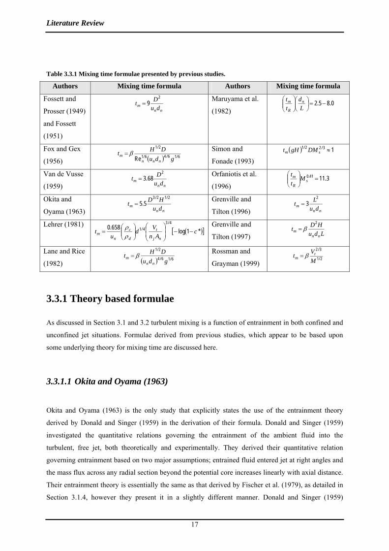
Literature Review
17
Table 3.3.1 Mixing time formulae presented by previous studies.
Authors Mixing time formula Authors Mixing time formula
Fossett and
Prosser (1949)
and Fossett
(1951)
nnm du
Dt2
9= Maruyama et al.
(1982) 0.85.2 −=⎟
⎠⎞
⎜⎝⎛⎟⎟⎠
⎞⎜⎜⎝
⎛Ld
tt n
R
m
Fox and Gex
(1956) ( ) 6/16/46/1
2/1
Re gduDHt
nnnm β=
Simon and
Fonade (1993) ( ) 13/22/1 ≈sm DMgHt
Van de Vusse
(1959) nnm du
Dt2
68.3= Orfaniotis et al.
(1996) 3.1141.0 =⎟⎟
⎠
⎞⎜⎜⎝
⎛s
R
m Mtt
Okita and
Oyama (1963) nnm du
HDt2/12/3
5.5= Grenville and
Tilton (1996) nnm du
Lt2
3=
Lehrer (1981) ( )[ ]*1log658.0
4/34/1 c
AnVd
ut
nj
t
d
c
nm −−⎟
⎟⎠
⎞⎜⎜⎝
⎛⎟⎟⎠
⎞⎜⎜⎝
⎛=
ρρ Grenville and
Tilton (1997) LduHDtnn
m
2β=
Lane and Rice
(1982) ( ) 6/16/4
2/1
gduDHt
nnm β=
Rossman and
Grayman (1999) 2/1
3/2
MVt t
m β=
3.3.1 Theory based formulae
As discussed in Section 3.1 and 3.2 turbulent mixing is a function of entrainment in both confined and
unconfined jet situations. Formulae derived from previous studies, which appear to be based upon
some underlying theory for mixing time are discussed here.
3.3.1.1 Okita and Oyama (1963)
Okita and Oyama (1963) is the only study that explicitly states the use of the entrainment theory
derived by Donald and Singer (1959) in the derivation of their formula. Donald and Singer (1959)
investigated the quantitative relations governing the entrainment of the ambient fluid into the
turbulent, free jet, both theoretically and experimentally. They derived their quantitative relation
governing entrainment based on two major assumptions; entrained fluid entered jet at right angles and
the mass flux across any radial section beyond the potential core increases linearly with axial distance.
Their entrainment theory is essentially the same as that derived by Fischer et al. (1979), as detailed in
Section 3.1.4, however they present it in a slightly different manner. Donald and Singer (1959)

Literature Review
18
propose that jet entrainment at right angles, means that entrained fluid has no momentum in the mean
jet flow direction before entering the jet and the conservation of momentum can be applied by
considering only the fluid across the inlet entrance and that passing through any transverse cross-
section of the jet, such that,
n
z
nnnz d
dQ
uQu =⇒=μμ . 3.3.1
The second assumption made by Donald and Singer (1959) was that the mass flux across any radial
section beyond the potential core increases linearly with axial distance, i.e.
zd z5.0tan =γ 3.3.2
where γ is the angle of jet spread, illustrated in Figure 3.1.1. The entrainment theory proposed by
Donald and Singer (1959) is derived by combining Equation 3.3.1 and 3.3.2.
constantcletd
zQ nn
===⇒ γγμ tan2,)tan2(
nn
Qdzc ⎟⎟⎠
⎞⎜⎜⎝
⎛=∴μ 3.3.3
Following the same method of mixing time evaluation as detailed in Section 3.2.1, Okita and Oyama
(1963) also derive that,
⎟⎠⎞
⎜⎝⎛
⎟⎟⎠
⎞⎜⎜⎝
⎛=
zH
dDT
nm
2
β 3.3.4
The major assumption that Okita and Oyama (1963) make after deriving Equation 3.3.4 is that the
effective entrainment distance, z, is equal to the tank diameter, D. They justify this assumption through
their experimental work, where it is concluded that the effect of nozzle angle has no effect on the
mixing characteristics within a tank. Thus, under the assumption of z=D in Equation 3.3.4, Okita and
Oyama (1963) find that the dimensionless mixing time formula is given by,
⎟⎠⎞
⎜⎝⎛
⎟⎟⎠
⎞⎜⎜⎝
⎛=
DH
dDT
nm
2
β . 3.3.5
The mixing time formula proposed by Okita and Oyama (1963) used Equation 3.3.5 as a basis, and re-
parameterised the D/dn and H/D ratios using experimental data. Okita and Oyama (1963), employed a
conductivity technique of measurement in their experimentation, where mixing time was defined as
Literature Review
19
the time between tracer addition and the moment when there were no differences in the concentration
measured by the two probes. With the re-parameterisation of Equation 3.3.5 with their experimental
work they proposed that the mixing time formula is,
5.02
⎟⎠⎞
⎜⎝⎛
⎟⎟⎠
⎞⎜⎜⎝
⎛=
DH
dDT
nm β . 3.3.6
The method employed by Okita and Oyama (1963) to derive their mixing time formula (Equation
3.3.6) fails in validity for two reasons: firstly, the application of free jet theory to confined jets, and
secondly, the assumption of entrainment distance being equal to tank diameter for all inlet
orientations. The inability to apply free jet theory is detailed in Section 3.2.2. The assumption of z=D,
is not correct for all inlet configurations. For example, the axial distance of the jet for a tank
configuration with a vertical feed and a large H/D ratio, is governed more by the height of the tank
than the diameter.
3.3.1.2 Lehrer (1981)
Lehrer (1981) developed a theoretical model for mixing of free, turbulent, buoyant jets, which he then
used to derive a mixing time formula. He claimed the mixing time formula he derived through free jet
principles was applicable to unimpeded jet flow over a given distance, after which the motion is too
slow for entrainment. Like most earlier free jet theoretical works (Fisher et al., 1979, Donald and
Singer, 1959), Lehrer (1981) assumed that there was a constant momentum rate in the direction of
mean flow where ambient fluid was entrained perpendicular to the mean flow. When his method is
applied to a case with no density differences, the entrainment model is essentially the same as that
derived by Donald and Singer (1959) (Equation 3.3.3), with the only difference being that Lehrer
(1981) quantifies the constant of proportionality to be equal to3
1 ,
nn
Qdz⎟⎟⎠
⎞⎜⎜⎝
⎛=
31μ . 3.3.7
Similarly to Equation 3.3.3, z in Equation 3.3.7 is the effective entrainment distance required for
complete mixing. Unlike other works, Lehrer (1981) determines the parameter z via theoretical
quantification. He defines z as the distance from the inlet where the jet power decreases to a limit,
beyond which motion is too slow to cause entrainment and thus, mixing.
Literature Review
20
The derivation for the characteristic equation (Equation 3.3.8 below) he uses to determine this distance
however is unclear.
3/1
limlim,⎭⎬⎫
⎩⎨⎧
⎟⎟⎠
⎞⎜⎜⎝
⎛= ititm x
contentsvesselofmassinputpoweru 3.3.8
In Equation 3.3.8, um,limit, refers to the maximum, centreline velocity at the effective entrainment
distance, xlimit. Lehrer (1981) finds for a case with no density differences, where the jet is unimpeded
over a distance of xlimit, the mixing time formula is,
4/34/9
*)1ln(658.0 ⎟⎠⎞
⎜⎝⎛
⎟⎟⎠
⎞⎜⎜⎝
⎛−−=
DH
dDcT
nm
4/34/9
⎟⎠⎞
⎜⎝⎛
⎟⎟⎠
⎞⎜⎜⎝
⎛=⇒
DH
dDT
nm β . 3.3.9
Where c* is the mixing criteria defined as,
)*exp(1*
0
0 tMccccc
tt
tt −−==−
− 3.3.10
in which M* is the mixing rate, ct0 is the initial concentration of an inject tracer when injected, ct is the
concentration of the tracer at the time of measurement and⎯ct is the mean tracer concentration in a
mixed system. Although some parts of Lehrer (1981)’s formula derivation is unclear, there is the
possibility of it accurately predicting mixing time under the given conditions. The problem lies
however in these formula conditions, i.e. an unimpeded flow over the length xlimit. In majority of the
experimental works, the tank aspect ratio and inflow jet velocities have been such that the criterion is
not met, and hence circulatory effects on mixing time are significant. Thus, the application of Equation
3.3.9 is almost impossible in reality.
Further, Lehrer (1981) shows support for his mixing time formula by showinge good correlation
between predicted mixing times and the experimental results of Fossett and Prosser (1949). However,
Lehrer (1981) makes no mention of testing the Fossett and Prosser tank configuration for wether the
jet is in fact unimpeded over xlimit. Furthermore, the accuracy of the experimental mixing times derived
by Fossett and Prosser (1949) has been criticised by later works such as Maruyama et al (1982), for
their tracer injection time constituting a large proportion of the record mixing time. Tracer injection
time needs to be kept short relative to the overall mixing time, to avoid injection influence on mixing
Literature Review
21
time (this is further discussed in Section 3.5.2.2). Hence, there is basically no evidence in the existing
literature surveyed, that show experimental support for Lehrer (1981)’s proposed mixing time formula.
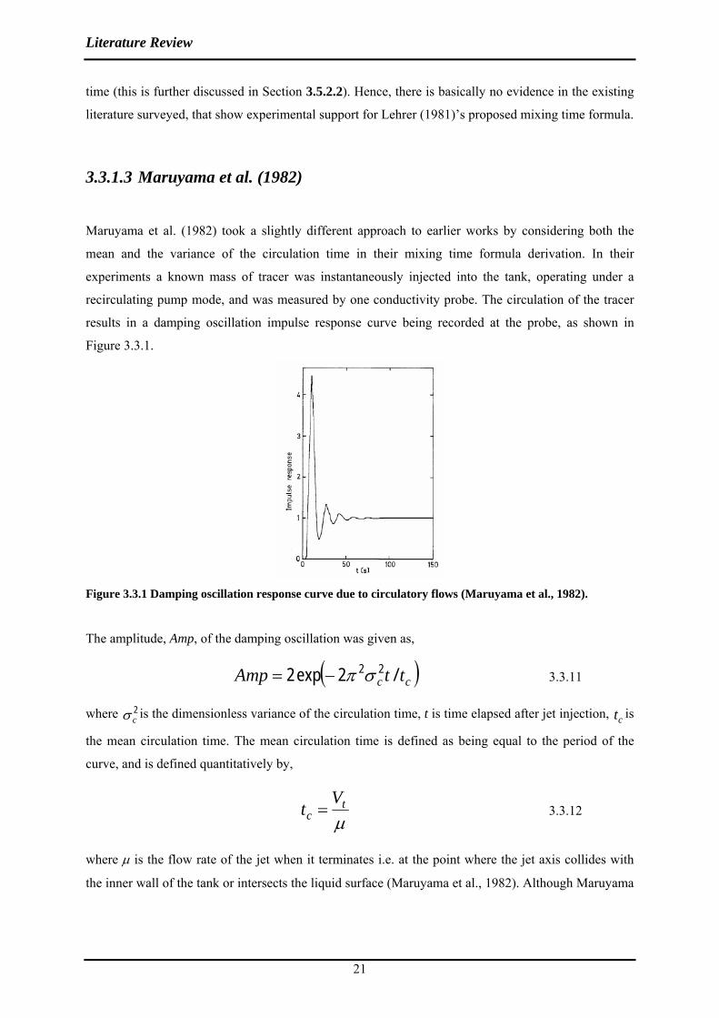
3.3.1.3 Maruyama et al. (1982)
Maruyama et al. (1982) took a slightly different approach to earlier works by considering both the
mean and the variance of the circulation time in their mixing time formula derivation. In their
experiments a known mass of tracer was instantaneously injected into the tank, operating under a
recirculating pump mode, and was measured by one conductivity probe. The circulation of the tracer
results in a damping oscillation impulse response curve being recorded at the probe, as shown in
Figure 3.3.1.
Figure 3.3.1 Damping oscillation response curve due to circulatory flows (Maruyama et al., 1982).
The amplitude, Amp, of the damping oscillation was given as,
( )cc ttAmp /2exp2 22σπ−= 3.3.11
where is the dimensionless variance of the circulation time, t is time elapsed after jet injection, is
the mean circulation time. The mean circulation time is defined as being equal to the period of the
curve, and is defined quantitatively by,
2cσ ct
μ
tc
Vt = 3.3.12
where μ is the flow rate of the jet when it terminates i.e. at the point where the jet axis collides with
the inner wall of the tank or intersects the liquid surface (Maruyama et al., 1982). Although Maruyama

Literature Review
22
et al. (1982) do not detail the exact source of their entrainment model, it is found to be of the same
form as that proposed by Donald and Singer (1959) (Equation 3.3.3),
nn
QdLc ⎟⎟⎠
⎞⎜⎜⎝
⎛=μ 3.3.13
for which L is defined as the free jet path length of the jet in tank (illustrated in the Figure 3.3.2
below). However, the free jet model used by Maruyama et al. (1982) differs from that proposed by
Donald and Singer (1959) in that, they assume z=L. As detailed in Section 3.2.2, the use of free jet
theory for confined jet situations induces much uncertainty to the validity of the proposed mixing time
formula. Note that unlike Okita and Oyama (1963), Maruyama et al. (1982) do not inaccurately
assume that the tank diameter, D, is an appropriate representation of effective entrainment distance for
all nozzle orientations.
Figure 3.3.2 Definition of free jet path length (Maruyama et al., 1982).
Combining Equation 3.3.12 and 3.3.13 produces,
cLQ
Vdtn
nc = 3.3.14
When t=tm the amplitude of the oscillation, Amp, is very close to zero, indicating a steady
concentration of tracer at the given measuring location within the tank. In Maruyama et al. (1982) the
value of tm for which the amplitude falls below a certain criterion is defined as the overall mixing time
for the whole tank. The criterion for such amplitude is not detailed however. Combining Equation
3.3.1.1 and 3.3.1.4 produces their mixing time formula,
⎟⎟⎠
⎞⎜⎜⎝
⎛⎟⎠⎞
⎜⎝⎛⎟⎠⎞
⎜⎝⎛
⎟⎟⎠
⎞⎜⎜⎝
⎛∝ 2
31c
n
nm L
dDH
dDT
σ. 3.3.15
Referring to Figure 3.3.3, Maruyama et al. (1982) find a lower mixing time for a circular jet (case a) in
comparison to a wall jet (case b). They use the inverse relationship between mixing time and variance
of circulation time given by Equation 3.3.15 to explain these experimental results on the effects of

Literature Review
23
nozzle location. Their explanation is that at the same mean circulation time, the circular jet produces
three-dimensional circulations with a larger variance of circulation time than a wall jet (because it only
induces two dimensional circulations with a small variance of circulation time) accounting for the
lower mixing time for a circular jet.
Figure 3.3.3 Circulation patterns induced for: (a) circular jet and (b) wall jet (Maruyama et al., 1982).
This explanation for the observed lower mixing time for a circular jet (Figure 3.3.3), fails due to a lack
of understanding of the jet mixing principles outlined in Section 3.2. Turbulent jet mixing, in confined
systems, occurs due to the formation of eddies, which entrain the ambient fluid into the jet fluid.
Circulation affects the rate of entrainment, but does not cause the mixing process itself. Thus, the
observations between a circular and wall jet are more accurately explained by the fact that the surface
area available for entrainment is much lower in the wall jet than that available in a circular jet. In other
words, it is the reduced entrainment rather than the variance of circulation time by the wall jet that
results in its higher mixing time. Furthermore, the variance of circulation time is not predictable prior
to experimentation and therefore Equation 3.3.15 is better represented as,
⎟⎠⎞
⎜⎝⎛⎟⎠⎞
⎜⎝⎛
⎟⎟⎠
⎞⎜⎜⎝
⎛=
Ld
DH
dDT n
nm
3
β . 3.3.16

Literature Review
24
3.3.1.4 Simon and Fonade (1993) and Orifaniotis et al. (1996)
Similar to previous studies, Simon and Fonade (1993) also used the conductivity technique to measure
mixing time. They tested configurations of one steady jet, two steady jets and two alternate
intermittent jets and found that regardless of configuration a constant mixing factor, close to the value
of one existed. They derive a mixing time formula under the argument that mixing time is function of
the specific momentum, Ms, and some reference time, tref, so that,
fs
refm M
tt ∝ 3.3.17
where f is some parameterisation of Ms, to be determined experimentally and,
gV
MMt
s ρ= 3.3.18
where M is the total momentum of all jets. They test the correlation between mixing time and various
parameters to determine how best tref can be represented. The parameters used to represent tref were:
the residence time, tR, the circulation time, tC, and the Reech-Froude similarity time, tFr, where;
n
tR Q
Vt = 3.3.19
( ) 2/1gH
DtFr = 3.3.20
3.3.21 singals alexpeirment from noscillatio of period=ct
When tm/tFr was plotted against Ms the strongest linear relationship was produced and hence they
replaced tref in Equation 3.3.17 with tFr, so that,
3/2s
F
m Mtt
∝ 3.3.22

Literature Review
25
Combining Equations 3.1.4, 3.3.18 and 3.3.22, the mixing time formula is derived as
3/73/11⎟⎟⎠
⎞⎜⎜⎝
⎛⎟⎠⎞
⎜⎝⎛=
nm d
DFr
T β 3.3.23
( ) 2/1gH
uFrwhere n= .
The method employed by Simon and Fonade (1993) was essentially purely empirical, although it is
presented in a manner that suggests otherwise, and thus it is present here in Section 3.3.1. Simon and
Fonade (1993) conducted their experiments under neutrally buoyant conditions. The Froude number is
a dimensionless number comparing inertial and gravitational forces. Therefore, the present study finds
the inclusion of the Froude number as an explanatory variable in the mixing time formula has no
physical meaning under neutrally buoyant situations.
Orfaniotis et al. (1996) extended the study of unsteady and steady jets initiated by Simon and Fonade
(1993). They investigated the effects of jet position and liquid viscosity. They found that provided the
flow generated inside the tank does not approach an impinging structure and no adjacent wall or free
surface exists in the region close to the nozzles, the location of the jet is not significant to mixing time.
In regards to the viscosity, it was found that mixing time increases with liquid viscosity. The mixing
time formula proposed by Orfaniotis et al. (1996) is essentially that proposed by Simon and Fonade
(1993) (Equation 3.3.23), modified to include the effects of fluid viscosity upon mixing. Their mixing
time formula is not investigated further as the only fluid considered in the present study is water.
3.3.1.5 Grenville and Tilton (1996, 1997)
The Grenville and Tilton (1996) paper is derived under the argument that the local turbulent kinetic
energy dissipation rate at the end of the free jet path controls the mixing rate for the whole vessel.
Grenville and Tilton (1996) prove this argument using the formula derived by Corrisin (1964), where
at high Schmidt numbers in low viscosity fluids mixing time is given by,
3/12
⎟⎟⎠
⎞⎜⎜⎝
⎛∝
εStm 3.3.24
where, S is the integral scale of concentration fluctuations and ε is the turbulent kinetic energy
dissipation rate. As S and ε need to be estimated, they then empirically tested various length scales and
ε values against the mixing time to determine the optimal parameter combination, i.e. producing the

Literature Review
26
highest correlation coefficient with the lowest standard deviation. It was found that parameter S was
best correlated to the free jet path length, L, and ε was best correlated to the turbulent kinetic energy
dissipation rate at the end of the free jet path, εz. Thus, substituting parameter S with L and ε with εz,
in Equation 3.3.24, the following mixing relation was produced
345.02
⎟⎟⎠
⎞⎜⎜⎝
⎛∝
zm
Ltε
. 3.3.25
The turbulent kinetic energy dissipation rate at some distance, z, from the source is given theoretically
by,
z
zz d
u 3∝ε 3.3.26
Similar to previous authors, Grenville and Tilton (1996) also employ the free jet theory in their
formula derivation (Equation 3.3.27 below), although they do not state the source or highlight that
they are applying free jet theory.
⎟⎠⎞
⎜⎝⎛=
zduu n
nz 6 3.3.27
Applying the conservation of momentum equation along the jet path,
nnzz dudu = 3.3.28
with Equations 3.3.25, 3.3.26 and 3.3.27, Grenville and Tilton (1996) propose the following mixing
time formula,
2297.2 ⎟⎟
⎠
⎞⎜⎜⎝
⎛=
nm d
LT . 3.3.29
They assumed that the aspect ratio effect is entirely captured by the free jet path length, L, although
this is only applicable somewhat to angled jets. Equation 3.3.29 was recorrelated in Grenville and
Tilton (1997) to include circulatory effects and in doing so, they captured the aspect ratio as separate
parameters in the mixing time formula (Equation 3.3.30 below) (Patwardhan and Gaikwad, 2003,
Wasewar, 2006, Zughbi and Rakib, 2002). The Grenville and Tilton (1997) study was not available for
detailed analysis in the present study.

Literature Review
27
⎟⎠⎞
⎜⎝⎛⎟⎠⎞
⎜⎝⎛
⎟⎟⎠
⎞⎜⎜⎝
⎛=
Ld
DH
dDkT n
jm
3
3.3.30
Where, ο
ο
158.131534.9
<=
>=
θ
θ
fork
fork
3.3.2 Other formulae
The majority of the existing formulae, other than those described in Section 3.3.1, investigated in the
present work are derived by dimensional analysis and purely empirical means. For this reason, the
method employed to derive a mixing time formula in these studies are not provided in detail. Instead, a
general description and key points about each of these other studies is presented in this section.
Fossett and Prosser (1949) and (1951) were the first to derive a jet mixing time formula. Water height,
H, was not considered as a parameter of mixing time in their proposed mixing time formula. They
studied the mixing of tetraethyl lead into aviation fuel in underground storage tanks via physical scale
modelling means. They employed conductivity technique to measure mixing time in a jet mixer. Their
experimental work was criticised by later works because their tracer injection time constituted
approximately 0.3-0.8 times the actual mixing time, and thus their mixing times were most likely to
have been overestimated. The effect of tracer injection time on recorded mixing times is detailed in
Section 3.5.2.2.
Fox and Gex (1956) studied jet mixing in both laminar and turbulent regimes and found that there was
a strong dependence of the mixing time on the jet Reynolds number in the laminar region and a only a
weak dependence in the turbulent region (defined at jet Reynolds numbers greater than 2000). In
comparison to Fossett and Prosser (1949), Fox and Gex (1949) included more parameters in their
mixing time formula, namely, the Reynolds number, Froude number and the water height. Their
general mixing time formula was derived by dimensional analysis. The provided justification for
parameter selection is insufficient and parameterisation of non-dimensional parameters was purely
empirical. Fox and Gex (1956) used visual observations of the acid-alkali neutralization reaction with
phenolphthalein indicator to measure mixing time produced from an inclined, side entry jet. This
visual measurement technique is criticised for its inaccuracy, supported by the finding of ±24% data
scatter in Fox and Gex (1956) results.
Van de Vusse (1959) also carried out studies on inclined, side entry jets. They measured mixing time
as the time from the start of the recirculation pump to the time when the densities of the samples

Literature Review
28
drawn from the tank were within a few per cent of the mean tank density. Unlike, Fox and Gex (1956)
they found that under a turbulent regime mixing time was independent of the jet Reynolds number.
They produced a mixing time formula very similar to that of Fossett and Prosser (1949) and likewise
exclude water height in their formula. Also similar to Fossett and Prosser (1949) they only preform
experiments over one tank aspect ratio.
Coldrey (1978) was the first to introduce the idea of the free jet length parameter (Lane and Rice,
1982). The free jet length was defined as the distance from the nozzle exit to where the jet impacts of a
tank boundary and was employed by later studies such as Maruyama et al. (1982) (Lane and Rice,
1982). He reported that a longer free jet length produces more effective mixing (Lane and Rice, 1982).
It was assumed that the mixing time is inversely proportional to the amount of liquid entrained by the
jet. An equation was proposed to empirically correlate the mixing time data (Lane and Rice, 1982).
Hiby and Modigell (1978) only tested axial, vertical jets located at the centre bottom of the tank. They
found the jet Reynolds number to be independent of mixing time when it was greater than 1x10⁶. They
formulated a mixing time equation similar in form to Fossett and Prosser (1949) and Van de Vusse
(1959), and likewise did not consider the height of the water in the tank to be an affecting factor to
mixing time. Hiby and Modigell (1978) were the first to clearly define mixing time by specifying the
degree of homogeneity required to define a well mixed system. They defined mixing time as the time
required to attain 95% homogeneity within the tank. This definition of mixing time is discussed in
detail in Section 3.5.1.
Lane and Rice (1981) investigated a vertical jet mixer in a vessel with a hemispherical base. They
found only very weak dependence of mixing time in the turbulent regime. Lane and Rice (182)
extended their investigations into side entry jets and also employed the same mixing time definition of
95% homogeneity as Hiby and Modigell (1978). They re-correlated the works of Fossett and Prosser
(1949, 1951) and Coldrey (1978) to produce a mixing time formulae of similar form to that derived by
Fox and Gex (1956). This mixing time formula proposed by Lane and Rice (1982) however is only
applicable to tank configurations that are equal to those of either Fossett and Prosser (1949, 1951) or
Coldrey (1978). They found that the Coldrey (1978) proposed tank design produced a lower mixing
time than that proposed by Fossett and Prosser (1949, 1951) and attributed this to Coldrey’s use of the
longest free jet path length.
Revill (1992) formulated an algorithm for jet mixer tank design based purely on the results derived
from previous works via a literature review. He recommended that:
o single axial jets should be used when the tank height to diameter (H/D) ratio is
between 0.7 and 3.0;
Literature Review
29
o side entry jets should be used when H/D is between 0.25 and 1.25;
o multiple side entry jets should be used when H/D is less than 0.25 or greater than 3.0;
and
o the jet should be orientated along the longest dimension of the tank.
However, his algorithm does not detail other tank configuration details such as nozzle diameter or
inflow jet velocity. Further he does not detail any investigation undertaken to test the validity of the
experimental works used for the derivation of his proposed algorithm.
Rossman and Grayman (1999) were the first to derive a mixing time formula for a tank operating
under the fill-and-draw tank operation mode. They re-parameterised the works of Okita and Oyama
(1963) and derived their mixing time formula by purely empirical means. Their experimental method
differed from Okita and Oyama (1963), in that:
1. the tracer was added with the external inflow instead of within the tank; and
2. a continuous feed tracer was used rather than a steep feed.
3.3.3 Generalised mixing time formula
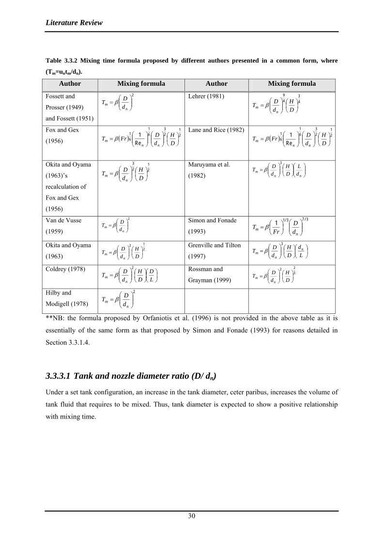
Section 3.3.1 and 3.3.2 highlight the numerous mixing time formulae presented by previous works and
details the derivation of the formulae. In this section however, the existing mixing time formulae are
collated into an initial generalised mixing time formula, and the each parameter is investigated for the
validity of its inclusion in the mixing formula employing jet flow fundamentals and existing
experimental evidence. Table 3.3.2, below, indicates that through the investigation into the derivation
of each pre-existing mixing time formula performed in Section 3.3.1 and 3.3.2, they can all be broken
down to the common structure,
cn
ba
nn
mnm L
dDH
dD
dtuT ⎟
⎠⎞
⎜⎝⎛
⎟⎠⎞
⎜⎝⎛
⎟⎟⎠
⎞⎜⎜⎝
⎛== β 3.3.31
The Reynolds number is not included in Equation 3.3.31 above, due to analogy with pipe flow. The
present study finds that within a fully turbulent regime mixing time should be independent of the
Reynolds number. The present study investigates only neutrally buoyant situations, and thus the
Froude number is also not included in Equation 3.3.31, as it has no physical significance under such
situations. The validation of the dimensionless ratios, D/dn, H/D and dn/L are more complex and are
hence discussed in detail in the following Sections, 3.3.3.1 to 3.3.3.3. A summary of the generalised
mixing time formula after investigation into the dimensionless ratios, D/dn, H/D and dn/L is presented
in Section 3.3.3.4.
Literature Review
30
Table 3.3.2 Mixing time formula proposed by different authors presented in a common form, where
(Tm=untm/dn).
Author Mixing formula Author Mixing formula
Fossett and
Prosser (1949)
and Fossett (1951)
2
⎟⎟⎠
⎞⎜⎜⎝
⎛=
nm d
DT β Lehrer (1981)
43
49
⎟⎠⎞
⎜⎝⎛
⎟⎟⎠
⎞⎜⎜⎝
⎛=
DH
dDT
nm β
Fox and Gex
(1956) ( ) 21
23
61
61
Re1
⎟⎠⎞
⎜⎝⎛
⎟⎟⎠
⎞⎜⎜⎝
⎛⎟⎟⎠
⎞⎜⎜⎝
⎛=
DH
dDFrT
nnm β
Lane and Rice (1982) ( ) 2
123
61
61
Re1
⎟⎠⎞
⎜⎝⎛
⎟⎟⎠
⎞⎜⎜⎝
⎛⎟⎟⎠
⎞⎜⎜⎝
⎛=
DH
dDFrT
nnm β
Okita and Oyama
(1963)’s
recalculation of
Fox and Gex
(1956)
21
23
⎟⎠⎞
⎜⎝⎛
⎟⎟⎠
⎞⎜⎜⎝
⎛=
DH
dDT
nm β
Maruyama et al.
(1982) ⎟⎟⎠
⎞⎜⎜⎝
⎛⎟⎠⎞
⎜⎝⎛
⎟⎟⎠
⎞⎜⎜⎝
⎛=
nnm d
LDH
dDT
3
β
Van de Vusse
(1959)
2
⎟⎟⎠
⎞⎜⎜⎝
⎛=
nm d
DT β Simon and Fonade
(1993)
3/73/11⎟⎟⎠
⎞⎜⎜⎝
⎛⎟⎠⎞
⎜⎝⎛=
nm d
DFr
T β
Okita and Oyama
(1963) 212
⎟⎠⎞
⎜⎝⎛
⎟⎟⎠
⎞⎜⎜⎝
⎛=
DH
dDT
nm β
Grenville and Tilton
(1997) ⎟⎠⎞
⎜⎝⎛⎟⎠⎞
⎜⎝⎛
⎟⎟⎠
⎞⎜⎜⎝
⎛=
Ld
DH
dDT n
nm
3
β
Coldrey (1978) ⎟⎠⎞
⎜⎝⎛⎟⎠⎞
⎜⎝⎛
⎟⎟⎠
⎞⎜⎜⎝
⎛=
LD
DH
dDT
nm
2
β Rossman and
Grayman (1999) 322
⎟⎠⎞
⎜⎝⎛
⎟⎟⎠
⎞⎜⎜⎝
⎛=
DH
dDT
nm β
Hilby and
Modigell (1978)
2
⎟⎟⎠
⎞⎜⎜⎝
⎛=
nm d
DT β
**NB: the formula proposed by Orfaniotis et al. (1996) is not provided in the above table as it is
essentially of the same form as that proposed by Simon and Fonade (1993) for reasons detailed in
Section 3.3.1.4.
3.3.3.1 Tank and nozzle diameter ratio (D/ dn)
Under a set tank configuration, an increase in the tank diameter, ceter paribus, increases the volume of
tank fluid that requires to be mixed. Thus, tank diameter is expected to show a positive relationship
with mixing time.
Literature Review
31
The effect of nozzle diameter on mixing time is a slightly more complicated. The power consumed
during the mixing process is from the dissipation of kinetic energy and is thus defined as,
322
821
nnnnn udQuP ρπρ =⎟⎠⎞
⎜⎝⎛= 3.3.32
.
When two nozzles of different diameter (dn,1 and dn,2) are operated at velocities un,1 and un,2,
respectively, in such a way that the power input by both is the same, the following relationship is
formed,
3/2
2,
1,
2,
1,
−
⎟⎟⎠
⎞⎜⎜⎝
⎛=
n
n
n
n
dd
uu
. 3.3.33
Combining Equation 3.3.31 with Equation 3.3.32,
3/2
2,
1,
2,
1,⎟⎟⎠
⎞⎜⎜⎝
⎛=
n
n
n
n
dd
MM
. 3.3.34
The above equations show that for a given power input, a larger nozzle diameter produces a larger
inflow momentum flux. As detailed in Section 3.2, entrainment and turbulent mixing is a positive
function of initial momentum flux. So, although the kinetic energy is the same initially in both cases, a
larger momentum flux means that a larger degree of turbulent mixing can occur. Therefore, according
to jet theory, mixing time and inlet diameter should have an inverse relationship.
Therefore, as D possesses a positive relationship with mixing time, and dn possess an inverse
relationship with mixing time, the D/ dn ratio is predicted, by jet theory principles, to have a positive
relationship with mixing time.
3.3.3.2 Tank height to diameter ratio (H/D)
As detailed in Section 3.3.3.1, an increase in tank diameter, D, ceter paribus, increases the volume of
tank fluid requiring mixing and thus, there is a positive relation between tank diameter and mixing
time. Similarly, an increase in the tank height, H, ceter paribus, also increases the volume of tank fluid
requiring mixing and thus, jet flow principles also predicts a positive relationship with mixing time.
Given that both H and D possess a positive relationship with mixing time, the relationship of the H/D
ratio with mixing time cannot be predicted by theory alone and experimental evidence is required.

Literature Review
32
3.3.3.3 Inlet diameter to free jet path length ratio (dn/L)
Applying the jet flow principles (detailed in Section 3.2) of entrainment it is expected that nozzle
angle and location effects mixing times to the extent that the jet interacts with the boundaries – solid
wall or free water surface. For neutrally buoyant situations in which all parameters except nozzle angle
and location are held constant, it is expected that jets with the same degree of jet impact or contact
with a boundary, will produce the same mixing time. Thus, a jet with a larger jet surface area available
for entrainment is predicted to produce better mixing than one with less, because it allows for a larger
surface area where turbulent mixing can occur.
It has been attempted to capture the effect of nozzle angle and location by the free jet path length
parameter, L, in previous studies, such as Coldrey(1978), Lehrer (1981), Maruyama et al (1982) and
Grenville and Tilton (1996, 1997). The problem with the use of free jet path length, L, by existing
works is that it has been interpreted as being equal to the distance between the inlet and the opposite
boundary (either tank wall or water surface), see Figure 3.3.2. The concept of “free” jet path length
has not been considered. For example, consider Figure 3.3.4 below. Under the existing literature’s
interpretation of free jet path length, cases (a) and (b) both have the same free jet path length.
However, ceter paribus, it is clear that according to jet theory principles case (a) should have a slower
mixing time due to the wall attachment of the jet, significantly reducing the surface area of the jet
available for entrainment. Also, given this common definition, the free jet path length for tall tanks
with a vertical, bottom inlet configuration can be overestimated, as the jet may lose most of its
momentum by the time it reaches the liquid surface.
Figure 3.3.4 Definition of free jet path length, L, for (a) centre, bottom, vertical feed inlet, and (b) side,
bottom, vertical feed inlet.
While jet theory principles indicate that parameter L can not capture nozzle angle and location effects,
the experimental evidence in the existing literature is also reviewed in the following Sections,
3.3.3.3.1 and 3.3.3.3.2 to gain further insight into the use of the parameter, L and the effects of nozzle
angle and location on mixing time.

Literature Review
33
3.3.3.3.1 Nozzle angle
Figure 3.3.5 Measurement of jet angle.
Okita and Oyama (1963) tested angles in the range of θ=0°-90°, where θ is the angle of nozzle
inclination from the horizontal (see Figure 3.3.5), and concluded that nozzle angle and location did not
have any significant influence on mixing time. Their results contain ±30 per cent data scatter and they
do not detail the results specific to each angle tested, and thus their work in this regard can not be
investigated further. Maruyama et al. (1982) tested nozzle angles over a range of 7°-73°. Maruyama
found that there is a strong relationship between mixing time and jet angle, with a 30° angle being
optimum for efficient mixing. Unlike Okita and Oyama (1963), Maruyama et al. (1982) place probes
after investigation of flow patterns within the tank via a visual measuring technique and thus, their
results are more reliable.
Dakshinamoorthy et al. (2006) uses the CFD modelling program, FLUENT, to investigate the effect of
nozzle angle using the tank configuration of Lane and Rice (1982). Dakshinamoorthy et al. (2006)
tested the nozzle angles of 30° and 45° against different nozzle diameters and found that mixing time
decreases as the nozzle diameter is increased for both angles of injection. Their results, presented in
Figure 3.3.6, indicated that both nozzle diameter and angle of injection had significant influence on
mixing time.
Figure 3.3.6 Influence of nozzle angle and diameter on mixing time (Dakshinamoorthy et al., 2006).

Literature Review
34
Zughbi and Rakib (2004) is the only work that extensively investigates the effect of nozzle angle and
diameter, and further presents findings in a sufficient detailed manner allowing for critical analysis by
the reader. However, Zughbi and Rakib (2004) do not discuss the reasoning behind their results in any
significant detail as is done so by the present study. While Dakshinamoorthy et al. (2006) only tests
for nozzle angles of 30° and 45°, Zughbi and Rakib (2004) conduct experiments for jet angles ranging
from 20° to 60°. Both works are in agreement that a 30° angle provides better mixing than a 45° angle.
Zughbi and Rakib (2004) find that the relationship between nozzle angle and mixing time is not a
monotone. Their results are shown in Figure 3.3.7. Qualitatively, this monotone relationship is
supported by works of Maruyama et al. (1984). Maruyama et al. (1984) observed a mixing time with a
local maximum at 0°, a local minimum between 25° to 30°, and a maximum from 45° to 50°, again a
local minimum at 75° and finally a maximum again at 90°.
Figure 3.3.7 CFD modelling mixing time results for various nozzle angles by Zughbi and Rakib (2004).
Application of confined jet theory principles, as discussed in Section 3.2. to the results of Zughbi and
Rakib (2004) suggests that mixing times at angles of 30° and 60° should be the same. This is because
at either angle, the jets have the same degree of jet impact/contact with a boundary, when all other
factors are held constant. However, Figure 3.3.7 shows that mixing time for a 60 ْ jet angle is
approximately 45 and 65% greater than that for a jet angled at 30 ْ, for jet Reynolds numbers 4000 and
5000, respectively. Thus, the results of Zughbi and Rakib (2004) do not agree with jet principles and
identical mixing times are not derived at angles of 30° and 60°. To examine the deviation from jet
theory prediction, the velocity profiles at each nozzle angle is investigated by the present study, and
presented in Figure 3.3.8. Observing Figure 3.3.8 it is apparent that at an angle of 60°, the outflow
position is causing plug flow conditions and wall attachment of the jet. Thus, the asymmetry between
nozzle angles of 30° and 60° is due to external factors such as the outflow position causing
experimental bias in the work of Zughbi and Rakib (2004). The experimental results of Patwardhan
and Gaikwad (2003), Figure 3.3.9, provide further experimental support for identical mixing times at
nozzle angles of 30° and 60°. The experimental set up of Patwardhan and Gaikwad (2003) is given in

Literature Review
35
(a)
(b)
Figure 3.3.8 Velocity profiles at nozzle angles of (a) 60° and (b) 30° (Zughbi and Rakib, 2004).
Figure 3.3.9 Mixing time results for various nozzle angles (Patwardhan and Gaikwad, 2003).
Contradictory to the works of Coldrey (1978), Lane and Rice (1982) and, Patwardhan and Gaikwad
(2003), Zughbi and Rakib (2004) did not find that a longest free jet path length angled at 45 ْproduces
Literature Review
36

Literature Review
37
(a)
(b)
Figure 3.3.10 Velocity profiles for nozzle angles of (a) 45° and (b) 30° (Zughbi and Rakib, 2004)

Literature Review
38
(a)
(b)
Figure 3.3.11 Velocity profiles for nozzle angles of (a) 20° and (b) 30° (Zughbi and Rakib, 2004).
3.3.3.3.2 Nozzle location
Zughbi and Rakib (2004) also investigated the effects nozzle location by altering the height of the inlet
for hi/H =0.2, 0.3 and 0.5, where hi is the distance from the base of the tank to the inlet nozzle.
Application of jet flow principles, suggests an inlet height half way down the tank, i.e. hi/H=0.5, will
produce the fastest mixing time, as also obtained by Maruyama et al. (1982). This is because there is
the least probability of wall attachment of the jet and hence the area available for entrainment is
maximised. However, Zughbi and Rakib (2004) results do not agree with this prediction, with the
nozzle orientated at hi/H=0.5 producing the slowest mixing time and the fastest mixing time is
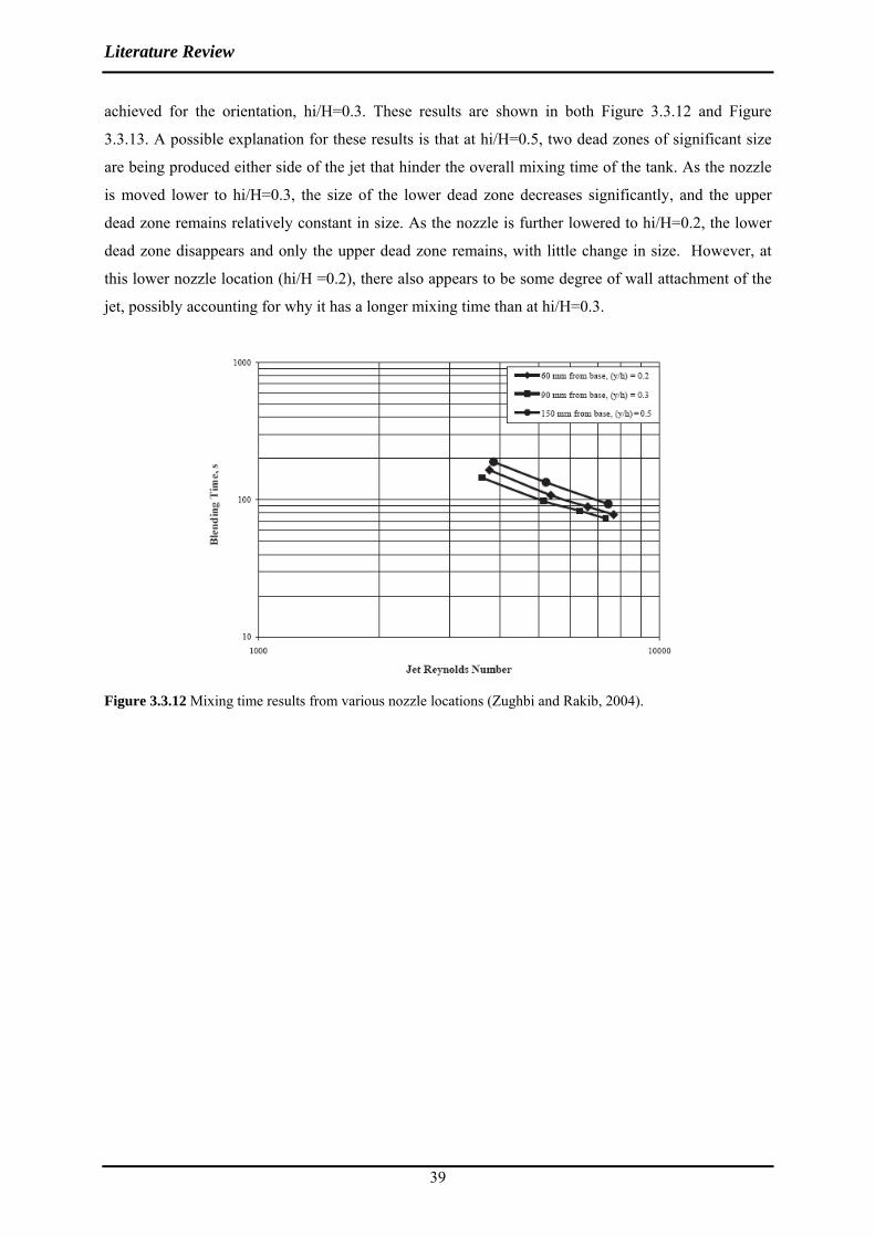
Literature Review
39
achieved for the orientation, hi/H=0.3. These results are shown in both Figure 3.3.12 and Figure
3.3.13. A possible explanation for these results is that at hi/H=0.5, two dead zones of significant size
are being produced either side of the jet that hinder the overall mixing time of the tank. As the nozzle
is moved lower to hi/H=0.3, the size of the lower dead zone decreases significantly, and the upper
dead zone remains relatively constant in size. As the nozzle is further lowered to hi/H=0.2, the lower
dead zone disappears and only the upper dead zone remains, with little change in size. However, at
this lower nozzle location (hi/H =0.2), there also appears to be some degree of wall attachment of the
jet, possibly accounting for why it has a longer mixing time than at hi/H=0.3.
Figure 3.3.12 Mixing time results from various nozzle locations (Zughbi and Rakib, 2004).
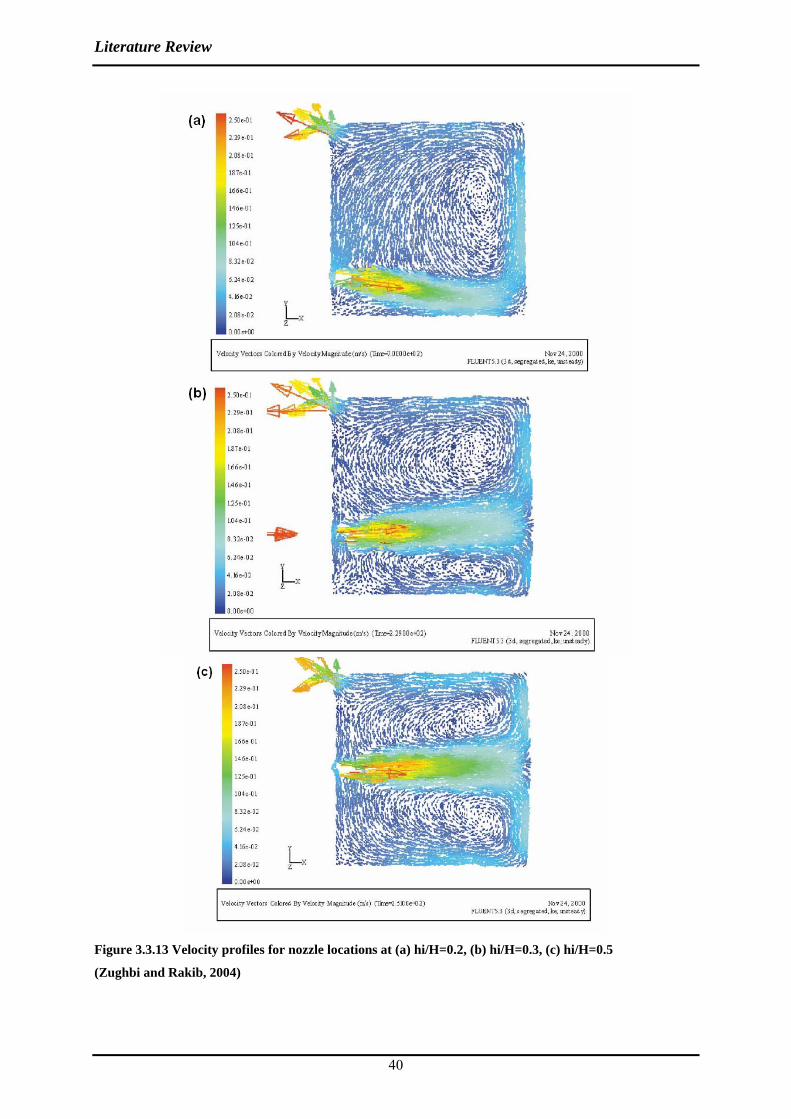
Literature Review
40
Figure 3.3.13 Velocity profiles for nozzle locations at (a) hi/H=0.2, (b) hi/H=0.3, (c) hi/H=0.5
(Zughbi and Rakib, 2004)
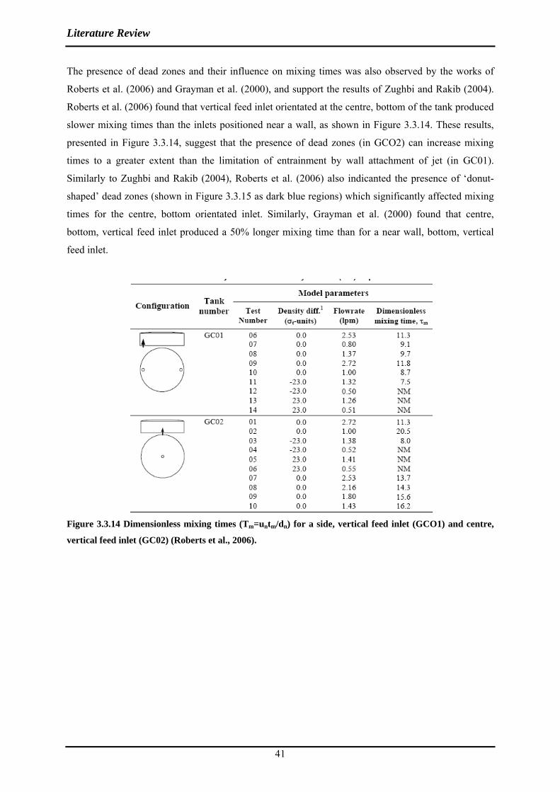
Literature Review
41
The presence of dead zones and their influence on mixing times was also observed by the works of
Roberts et al. (2006) and Grayman et al. (2000), and support the results of Zughbi and Rakib (2004).
Roberts et al. (2006) found that vertical feed inlet orientated at the centre, bottom of the tank produced
slower mixing times than the inlets positioned near a wall, as shown in Figure 3.3.14. These results,
presented in Figure 3.3.14, suggest that the presence of dead zones (in GCO2) can increase mixing
times to a greater extent than the limitation of entrainment by wall attachment of jet (in GC01).
Similarly to Zughbi and Rakib (2004), Roberts et al. (2006) also indicanted the presence of ‘donut-
shaped’ dead zones (shown in Figure 3.3.15 as dark blue regions) which significantly affected mixing
times for the centre, bottom orientated inlet. Similarly, Grayman et al. (2000) found that centre,
bottom, vertical feed inlet produced a 50% longer mixing time than for a near wall, bottom, vertical
feed inlet.
Figure 3.3.14 Dimensionless mixing times (Tm=untm/dn) for a side, vertical feed inlet (GCO1) and centre,
vertical feed inlet (GC02) (Roberts et al., 2006).

Literature Review
42
Figure 3.3.15 Donut shaped dead zones for centre, vertical feed inlets (Roberts et al., 2006)
It should be noted that the effects of nozzle location have not been explained or discussed in detail in
neither Grayman et al. (2000), Zughbi and Rakib (2004) or Roberts et al. (2006). Zughbi and Rakib
(2004) do not provide any explanation or discussion of their results beyond highlighting circulation
patterns have a significant effect on mixing times. Similarly, Roberts et al. (2006) merely recommend
that vertical inlet should be positioned near the tank wall to eliminate the production of such donut-
shaped dead zones.
Further analysis by Roberts et al. (2006) into these donut-shaped dead zones, find that the size of the
dead zones are significantly reduced by an increase in initial jet velocity as shown in Figure 3.3.16.
Their results as shown in Figure 3.3.14, show that the difference in mixing times between the inlet
configurations is more pronounced at low flow rates, however at high flow rates such as 2.53 and 2.72
lpm (litres per minute) both tanks produce similar dimensionless mixing times of 11.3.
Figure 3.3.16 Effect of inflow rate on the size of dead zones (Roberts et al., 2006).
Literature Review
43
3.3.3.3.3 Summary
Experimental evidence on the effects of nozzle angle and location, have been conflicting and
unexplained. The present study analyses this unexplained experimental evidence from previous studies
on nozzle angle and location to find that consistent conclusions can be drawn from previous
experimental study results and jet flow principles. In particular, there is agreement between principles
of jet flow and experimental evidence from previous studies that jets with the same degree of impact
with a boundary will produce similar mixing times, ceter paribus. In regards to nozzle location, it is
found that the size and presence of dead zones can significantly differ to the predictions made by jet
flow principles. Therefore, experimental evidence indicates that the effect of jet angle and location is a
function of many factors such as: free jet path length (L), proximity to boundaries, interaction with
boundaries, velocity of circulatory flows and circulatory flow patterns. Thus, the free jet path length
parameter, L, alone can not explain or capture the effects of inlet nozzle angle and/or location. It also
appears that the differences in mixing times between various inlet configurations is less pronounced at
higher jet inflow velocities.
Therefore, given the present state to knowledge, the free jet path length parameter can not capture the
effect of various inlet configurations on mixing time and hence the dn/L parameter should not be
included in the mixing time formula. Further, a parameter/s that does capture the effects of various
inlet configurations on mixing time is/are not available at present due to the inability to quantify and
predict: the degree of jet interaction with a boundary; velocity of circulatory flows; the circulatory
flow patterns; and the relation between each of these influencing factors.
3.3.3.4 Summary
Sections 3.3.3.1 and 3.3.3.2 indicate that both D/dn and H/D are important dimensional ratios
governing mixing time. The free jet parameter legth, L, which is used to capture the effect of nozzle
angle and location, however is proved to be an ineffective measure of inlet configuration in Section
3.3.3.3. Thus, the parameter L, and consequently the ratio dn/L, is not included in the proposed
generalised mixing time formula (Equation 3 below), derived from the application of jet flow
fundamentals and existing experimental evidence.
cn
ba
nn
mnm L
dDH
dD
dtuT ⎟
⎠⎞
⎜⎝⎛
⎟⎠⎞
⎜⎝⎛
⎟⎟⎠
⎞⎜⎜⎝
⎛== β 3.3.35
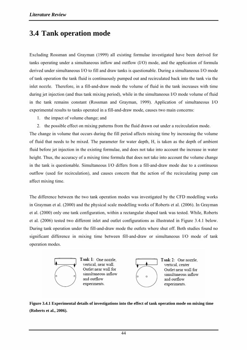
Literature Review
44
3.4 Tank operation mode
Excluding Rossman and Grayman (1999) all existing formulae investigated have been derived for
tanks operating under a simultaneous inflow and outflow (I/O) mode, and the application of formula
derived under simultaneous I/O to fill and draw tanks is questionable. During a simultaneous I/O mode
of tank operation the tank fluid is continuously pumped out and recirculated back into the tank via the
inlet nozzle. Therefore, in a fill-and-draw mode the volume of fluid in the tank increases with time
during jet injection (and thus tank mixing period), while in the simultaneous I/O mode volume of fluid
in the tank remains constant (Rossman and Grayman, 1999). Application of simultaneous I/O
experimental results to tanks operated in a fill-and-draw mode, causes two main concerns:
1. the impact of volume change; and
2. the possible effect on mixing patterns from the fluid drawn out under a recirculation mode.
The change in volume that occurs during the fill period affects mixing time by increasing the volume
of fluid that needs to be mixed. The parameter for water depth, H, is taken as the depth of ambient
fluid before jet injection in the existing formulae, and does not take into account the increase in water
height. Thus, the accuracy of a mixing time formula that does not take into account the volume change
in the tank is questionable. Simultaneous I/O differs from a fill-and-draw mode due to a continuous
outflow (used for recirculation), and causes concern that the action of the recirculating pump can
affect mixing time.
The difference between the two tank operation modes was investigated by the CFD modelling works
in Grayman et al. (2000) and the physical scale modelling works of Roberts et al. (2006). In Grayman
et al. (2000) only one tank configuration, within a rectangular shaped tank was tested. While, Roberts
et al. (2006) tested two different inlet and outlet configurations as illustrated in Figure 3.4.1 below.
During tank operation under the fill-and-draw mode the outlets where shut off. Both studies found no
significant difference in mixing time between fill-and-draw or simultaneous I/O mode of tank
operation modes.
Figure 3.4.1 Experimental details of investigations into the effect of tank operation mode on mixing time
(Roberts et al., 2006).
Literature Review
45
Therefore it is concluded that in the present study, the application of formulae derived from
simultaneous I/O mode experiments to tanks operating under a fill-and-draw mode is not limited by
the operational mode used for the particular formula derivation.
3.5 Experimental Method Evaluation
In this section, the experimental issues regarding mixing time measurement are discussed, so as to
guide future experimental works.
3.5.1 Definition of mixing time
Mixing time tm, is defined in most previous studies uses the Coefficient of Variation (COVt) to define
a criterion for mixing time. COVt is defined as the time when the tracer concentration, Ct, at the
measurement location has reached, or has nearly reached, the expected final mean tracer
concentration, C t . The formula for COVt in probe measurement applications is defined as,
tt
tt COVC
CC=
− 3.5.1
where t
tnt V
CQC 0,= , and C t,0 is the initial tracer concentration.
COVt =1.0 at the start of the mixing process, and COVt =0 when complete homogeneity has been
achieved (Revill, 1992). As complete homogeneity is not able to be practically measured, most studies
use a mixing time criterion for ranging from 0.01 to 0.1. The use of COVt to determine mixing time is
illustrated in Figure 3.5.1 (Revill, 1992).

Literature Review
46
Figure 3.5.1 Chart recorder plot of a conductivity trace after addition of a tracer (Lane and Rice, 1982).
3.5.2 Probe measurement
Majority of the work in the field of jet mixing within confined systems has been conducted by
physical scale modelling. Thus, this experimental method needs to be evaluated so as to evaluate the
accuracy of the experimental evidence from previous studies and to guide future experimental works.
3.5.2.1 Point source measurement
Probe measurement is a point source measurement technique and thus is unable to capture the flow
patterns of interest in tank mixing applications. Probe measurement is ineffective unless probes are
placed in known, poorly mixed regions, identified by means such as flow visualisation, and even still
are unable to capture the size of the poorly mixed region (Jayanti, 2001). Jayanti (2001) investigated
the effects of probe location and overall mixing time. The different probe positions produced a wide
range of results, ranging from 60 to 300 seconds for experiments run under the same tank operating
conditions. Revill (1992) also found that the measurement probes themselves can interfere with the
flow in the tank. Similarly, the size of the probes were also found to interfere with the flow, where the
bigger the probe, the shorter the recorded mixing time. Thus, in the selection of the number of probes,
there is a tradeoff between, the number of measurements capturing the flow field and the alteration of
the flow field.
Literature Review
47
3.5.2.2 Tracer injection time
Fossett (1951) and Yianneskis (1991) both find that overall mixing time is positively correlated to
tracer injection time. A criterion for specifying how to determine the acceptable tracer injection time
however is not specified by either of the works. Shorter injection times are thus preferred, and need to
be taken into account when analysing the validity of various physical scale experimental works.
Unfortunately majority of such experimental works do not specify the injection time period used. The
inability to validate experimental works according to injection time is one drawback of the present
work.
3.5.2.3 Tracer injection location
The dependence of the measured mixing time to tracer input location has only been studied by
Dakshinamoorthy et al. (2006). They found that overall mixing time was dependent on tracer input
location, and this dependence was most pronounced in low Reynolds number cases. The explanation
behind this observation being, lower mixing times are achieved when tracer is injected into high
velocity regions due to re-circulation effects. Similarly, higher mixing times are obtained when tracer
injection is in areas of low velocity (at the extreme dead zones), where the absence of re-circulation
causes the tracer to be trapped within the boundaries of the low flow zone area. To exclude the effects
of tracer injection time and tracer location Dakshinamoorthy et al. (2006) suggest the tracer is injected
into the inflow itself via a short injection time.
3.6 Existing Guidelines
The only comprehensive collation of existing works into the field of tank mixing and development of
guidelines has been produced by Grayman et al. (2000). Grayman et al. (2000) collate the results of
various projects that have been conducted by the American Water Works Association Research Fund
(AWWARF) into water quality in water distribution tanks and reservoirs, and produce a set of general
guidelines.
Although the work of Grayman et al. (2000) has been extensive, it has been concentrated to evaluating
the extent of mixing and mixing characteristics of existing water storage facilities and temperature
effect studies. Useful investigative work has been conducted via CFD modelling on the effects of
nozzle location, where models are validated against existing field data. Their tank design guidelines
are based on the mixing time formula derived by Rossman and Grayman (1999), most likely because
the work of Rossman and Grayman (1999) was conducted under the AWWRF. They do not however

Literature Review
48
investigate the derivation of neither the Rossman and Grayman (1999) formula nor the various mixing
time formulae available. Rossman and Grayman (1999) parameterise the general mixing time formula
derived by Okita and Oyama (1963) from physical modelling tests using only two aspect ratio tanks
and tank to nozzle diameter ratios. For other tank configurations the validity of the Rossman and
Grayman (1999) formula needs to be further tested.
3.7 Supporting Experimental Works
A number of experimental works conducted via both, physical scale modelling and Computational
Fluid Dynamic (CFD) modelling, have also investigated the issue of tank mixing. These studies do not
derived a mixing time formulae, but instead investigate various aspects of tank mixing. Such physical
scale modelling works include: Grayman et al. (2000), Patwardhan and Gaikwad (2003) and
Patwardhan et al. (2003) and Roberts et al. (2006). With the development and increasing acceptance of
CFD modelling as a valid form of experimentation, the application to tank mixing has been prominent
in recent years. However, majority of the CFD modelling works have investigated tank mixing using
impeller blades rather than jet mixers (Jayanti, 2001). Further, CFD modelling works that do
investigate jet mixers such as; Brooker (1993), Hoffman (1996), Jayanti and Pavithra (1996), Ranade
(1996), Wasewar and Patwardhan (2002), and Patwardhan (2002), focus on justifying the use of CFD
modelling for jet mixing within tank applications, but provide little investigation into the effect of tank
parameters on mixing time. The resulting set of CFD works that actually provide useful information
for the purposes of the present study are limited. Such works include; Jayanti (2001), Rakib and
Zughbi (2002, 2004) and Dakshinamoorthy et al. (2006). These works are independent of each other
and have not been integrated or analysed in detail with the other existing experimental works and
formulae, prior to the present study.

Methodology
49
4 Methodology
The present work was undertaken in two primary stages; critical analysis of existing relevant literature
and CFD modelling, in order to produce a generalised mixing time formula.
The CFD modelling was dependent upon the findings of the literature review stage. From the literature
review stage the parameters, parameter ranges and tank configurations where data was lacking or
deemed as requiring more, were conducted in the CFD modelling stage.
4.1 Review of historical results and data
The existing literature on jet flow principles, experimental studies and supporting experimental works
is reviewed and analysed firstly to determine a generalised mixing time formula and the range of
parameters required for further testing in the CFD program, CFX. The principles behind free jet theory
and the differences to confined jet situations is investigated firstly. Conclusions are then drawn on the
principles governing jet flow and entrainment rate in confined jet situations, and are applied to the
analysis of the existing mixing time formulae produced by previous studies. Experimental measuring
methods are also investigated, specifically probe measurement, so as to analyse the experimental
validity of the results produced by previous studies. It is found that the mixing time of previous studies
could be collated into the form,
cn
ba
nn
mnm L
dDH
dD
dtuT ⎟
⎠⎞
⎜⎝⎛
⎟⎠⎞
⎜⎝⎛
⎟⎟⎠
⎞⎜⎜⎝
⎛== β 4.1.1
where a, b and c are unknown parameterisation constants, and β is also a constant. Experimental
evidence and confined jet principles are then applied to each of the dimensional ratios presented in
Equation 4.1.1 to determine to validate its inclusion in the mixing time formula.

Methodology
50
From this analysis, it is determined that although inlet configuration has an effect on mixing time it
can not be captured by the free jet path length parameter, L, and the dimensional mixing time is more
correctly represented by,
ba
nn
mnm D
HdD
dtuT ⎟
⎠⎞
⎜⎝⎛
⎟⎟⎠
⎞⎜⎜⎝
⎛== β . 4.1.2
The dimensionless ratios of D/dn and H/D from Equation 4.1.2 are then plotted against dimensional
mixing time, Tm, using experimental data derived and collated for previous studies, to determine the
parameterisation constants a and b. As the review of these graphical results indicated that sufficient
data existed in the present literature to determine the parameterisation constant, a, no further testing of
D/dn ratios via CFD modelling is undertaken. However, this review also indicated that an insufficient
data set for H/D ratios was present to accurately determine the constant, b, in the existing literature. It
is thus decided that a data set spanning H/D ratios over the range of 0.3 to 3 are required to be
generated by the means of numerical results. The inlet configuration for the CFD modelling stage was
chosen to be a vertical feed inlet at the centre, bottom of the tank. The inlet configuration was chosen
to be of radially symmetrical to the tank so as to minimise the effects of nozzle angle and location
upon mixing time. A radially symmetrical tank configuration produces a base case data set which
allows for a more accurate measure of the influence of the H/D and D/dn ratios on mixing time,
without the potential for data bias caused by capturing effects of inlet orientation and asymmetrical
flows.
4.1.1 Limitations
The three main limitations faced during the review of historical results and data is:
1. Limited data base. Although the earliest work specific to jet mixing and mixing time by
Fossett and Prosser was performed in 1949, there has not been a significant amount of
research into jet mixing. This is because jet mixing has not traditionally received much focus,
with research interests dominated more toward impeller and mechanical agitator systems.
Mixing research has been focused to the chemical processing industries where the material is
often sludge-like and therefore is more appropriately mixed with impellers or mechanical
agitators.
2. Accessibility of literature. Some of the research papers that were of interest were not able to
be retrieved. For works which were not available through the University of Western

Methodology
51
Australia’s Library and Inter-loan service, attempts to contact the authors directly were
conducted. The papers of particular interest that were not accessible are Coldrey (1978) and
Grenville and Tilton (1997)
3. Limited disclosure. The limited disclosure of the experimental method and results produces
difficulty in accurately analysing the validity of the paper and its results, in much of the
literature reviewed. Limited disclosure of experimental details also meant that the data base
used for determining the parameterisation constants was limited.
4.2 CFD modelling
4.2.1 Overview
The software program, GAMBIT, was used to generate the tank geometry and mesh, which are then
imported into the CFD program, CFX 11.0. CFX is used to run each of the required simulations. The
CFD program, CFX was chosen as it is found to be the best program available at the time of the
present study for tank mixing applications (pers. comm. Thomas Ewing). CFX is designed to import
from the program GAMBIT, and was hence the reasoning for the use of GAMBIT.
GAMBIT was used to generate the tank geometry and meshing, and each simulation was run in the
CFD modelling program, CFX. A step-wise overview of the methodology undertaken for the CFD
modelling stage of the present study is detailed here.
1. An appropriate experimental data set for model validation is investigated and Roberts et al.
(2006) is chosen. Details of the selection of Roberts et al. (2006) experimental data set is
presented in Section 4.2.2.1.
2. In the process of validating CFD model with experimental data of Roberts et al. (2006), errors
in the measurement of mixing time by Roberts et al. (2006) were discovered. The presence of
these errors inhibits the complete validation of mixing times derived by the CFD model with
the mixing times recorded in the experimental data of Roberts et al. (2006). Given the vast
support for the accuracy and reliability of CFD models (as discussed in Section 3.6), it is
concluded that running of the CFD model without experimental data validation should not be
a significant limitation to the present study. Further, other existing experimental data disclosed
in sufficient detail for use in model validation, is not available. Hence, it is decided that the

Methodology
52
model be run for the required simulations without further attempts at model validation via
experimental data. This is discussed in detail in Section 4.2.2.2 and 4.2.2.3.
3. Validation of the numerical results produced by the model is instead conducted qualitatively
conducted through comparison of tracer plots. For this, a simulation for a half tank, with a
plane of symmetry along the x-axis, is conducted under the same set of initial conditions as for
an experimental run conducted by Roberts et al. (2006). As it is found that the CFD results
produced the expected tracer concentration profiles, and symmetry of flow exists around the z-
axis, the tank was cut down to a smaller slice. The model specifications are detailed in Section
4.2.3.
4. A new geometry and mesh is created for each required simulation in GAMBIT. Each
simulation is imported in Pre-CFX 11.0, run in CFX-Solver 11.0, and the mixing time is
determined in the post-processor , CFX-Post 11.0. Simulation details are provided in Section
4.2.4.
4.2.2 Validation of numerical results
The details for the selection of the experimental data used for the validation of the numerical results,
the problems attained during the process of numerical validation and the conclusions derived for the
whole process are detailed in this section.
4.2.2.1 Experimental data selection
Simulations conducted via CFD modelling are often validated against a set of physical scale or field
experimental data to ensure there is no discrepancy between the two and hence ensures the accuracy
and reliability of the CFD results. In the present study, the experimental work by Roberts et al. (2006)
is chosen initially for validating the CFD simulations. The Roberts et al. (2006) work was selected for
model validation for three primary reasons:
1. It is the only comprehensive physical scale experimental work that clearly details the initial
conditions and results of each simulation conducted;
2. The present study was required to be run under fill-and-draw tank operational mode, which
was also the tank operational mode employed in Roberts et al. (2006); and
3. The mixing times produced are believed to be of much higher accuracy as the entire flow field
is analysed when determining the mixing times compared to the mixing times produced by
majority of the existing, probe measured, physical scale experimental works.

Methodology
53
Roberts et al. (2006) conducted experimental work using a technique called, Three-Dimensional Laser
Induced Fluorescence (3DLIF). The 3DLIF method can measure the whole filed of tracer
concentrations in the tanks and its temporal evolution through the mixing process (Roberts et al.,
2005). The experimental set up consists of two fast scanning mirrors that drive a laser beam through
the flow in a programmed pattern (Roberts et al., 2005). The fluorescent dye, Rhodamine 6G, is added
to the inflow (Roberts et al., 2005). The laser causes the dye to fluoresce, and the emitted light is
captured by a camera and processed in the connected computers (Roberts et al., 2005). A schematic of
this experimental procedure is shown in the Appendix, Section 10. Roberts et al. (2006) choose a
mixing time criterion of COV<10% rather than the 5% used by most other studies, in accordance to
the aims specific to their study.

Methodology
54
4.2.2.2 Problems with model validation
Attempts to validate the mixing times derived by the numerical model with the experimental works of
Roberts et al. (2006) were hindered by the discovery that the measuring method employed by Roberts
et al. (2006), contrary to initial thought, did not actually evaluate the entire flow field. The validation
was attempted by regenerating an exact experiment performed by Roberts et al. (2006) where the
mixing time was approximated to be 74 seconds. In the numerical model, the mixing time is evaluated
on the plane of symmetry for a half tank geometry, as illustrated in Figure 4.2.2. The mixing time
derived by the numerical model, is much longer than 74 seconds, at approximately 120 seconds. With
closer observance of the Roberts et al. (2006) data, it is discovered that the scanning planes only
captured the flow field at the initial water height, and the evaluation plane did not increase in height
with respect to the increase in tank volume during the fill period. The ignorance of the entire flow field
is evident as the tracer concentration plot for a fully mixed tank in Figure 4.2.1 is taken only to the
initial height of 0.11 meters. Figure 4.2.2 produced from the CFX program, shows that by only
considering the initial height (indicated by the horizontal grey plane), Roberts et al. (2006) do not
taken into account the effects of tracer recirculation immediately after jet impact of the free surface.
As observed in Figure 4.2.2, the variation in tracer concentrations is significant in the flow field region
above the initial height of 0.11 meters. The numerical model’s ability to capture and evaluate the
entire flow plane explains why the mixing times derived the model are larger than that given by
Roberts et al. (2006).
Figure 4.2.1 Tracer concentration profiles produced by Roberts et al. (2006) for a mixed tank.
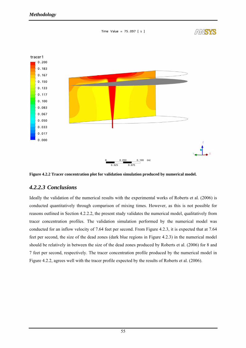
Methodology
55
Figure 4.2.2 Tracer concentration plot for validation simulation produced by numerical model.
4.2.2.3 Conclusions
Ideally the validation of the numerical results with the experimental works of Roberts et al. (2006) is
conducted quantitatively through comparison of mixing times. However, as this is not possible for
reasons outlined in Section 4.2.2.2, the present study validates the numerical model, qualitatively from
tracer concentration profiles. The validation simulation performed by the numerical model was
conducted for an inflow velocity of 7.64 feet per second. From Figure 4.2.3, it is expected that at 7.64
feet per second, the size of the dead zones (dark blue regions in Figure 4.2.3) in the numerical model
should be relatively in between the size of the dead zones produced by Roberts et al. (2006) for 8 and
7 feet per second, respectively. The tracer concentration profile produced by the numerical model in
Figure 4.2.2, agrees well with the tracer profile expected by the results of Roberts et al. (2006).
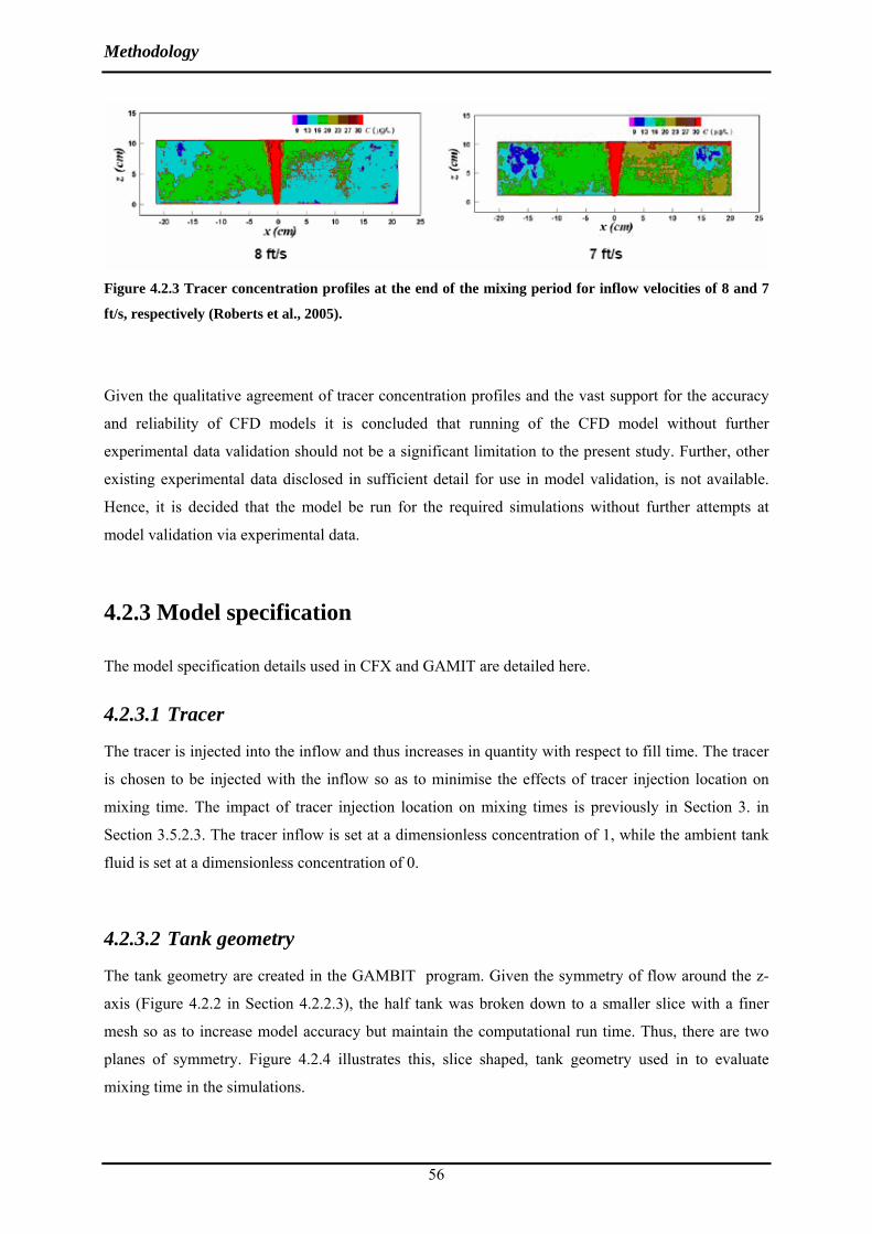
Methodology
56
Figure 4.2.3 Tracer concentration profiles at the end of the mixing period for inflow velocities of 8 and 7
ft/s, respectively (Roberts et al., 2005).
Given the qualitative agreement of tracer concentration profiles and the vast support for the accuracy
and reliability of CFD models it is concluded that running of the CFD model without further
experimental data validation should not be a significant limitation to the present study. Further, other
existing experimental data disclosed in sufficient detail for use in model validation, is not available.
Hence, it is decided that the model be run for the required simulations without further attempts at
model validation via experimental data.
4.2.3 Model specification
The model specification details used in CFX and GAMIT are detailed here.
4.2.3.1 Tracer
The tracer is injected into the inflow and thus increases in quantity with respect to fill time. The tracer
is chosen to be injected with the inflow so as to minimise the effects of tracer injection location on
mixing time. The impact of tracer injection location on mixing times is previously in Section 3. in
Section 3.5.2.3. The tracer inflow is set at a dimensionless concentration of 1, while the ambient tank
fluid is set at a dimensionless concentration of 0.
4.2.3.2 Tank geometry
The tank geometry are created in the GAMBIT program. Given the symmetry of flow around the z-
axis (Figure 4.2.2 in Section 4.2.2.3), the half tank was broken down to a smaller slice with a finer
mesh so as to increase model accuracy but maintain the computational run time. Thus, there are two
planes of symmetry. Figure 4.2.4 illustrates this, slice shaped, tank geometry used in to evaluate
mixing time in the simulations.

Methodology
57
Figure 4.2.4 Illustration of the type of tank geometry used in the numerical modelling process.
The tank wall, tank bottom, and nozzle are specified as no-slip, no-flow boundaries. The bottom of the
nozzle is specified as the inlet. The nozzle is extended to 0.025 metres from the tank bottom, for all
simulations, as it is deemed of sufficient length to produce the necessary pipe flow regime within the
nozzle (pers. comm. Thomas Ewing). There is no nozzle protrusion into the tank.
The top liquid surface is specified as a free-slip, no-flow boundary, which moves along the z-axis by a
user-defined function specifying the height increase velocity of the tank with respect to time. The
height increase velocity is specified as,
π4 velocity increaseheight 2 ×=
DQn . 4.2.1
The top liquid surface is simulated as a flat interface, as is done in all the investigated CFD works
performed for confined jet flow. This assumption of a flat surface is primarily chosen for
computational convenience, i.e. to minimize complexity of model set up and to minimize model run
time. Further, incorporation of the fluctuations of the top liquid surface requires enormous amounts of
body fitted grids and unsteady state modelling and is estimated to have minimal impact on the overall
mixing times (pers comm. Thomas Ewing).
Methodology
58
4.2.3.3 Meshing
GAMBIT 2.0 was also used to generate the grid (mesh) each tank required to be tested in the
numerical model. Hexahedral shaped cells were chosen, rather than tetrahedral, as they provide for
more accurate numerical evaluation (Jayanti, 2001). The mesh size is varied throughout the tank. Fine
meshing was used within the nozzle and extended to the top liquid surface, so as to ensure both pipe
flow within the nozzle, and the complex flow within the jet are captured accurately by the model. The
cell size is set to increase by 2 per cent along the z-axis from the bottom to the top of the tank. This is
because jet flow principles detailed indicate that more complex flows are expected in the region of
flow development near the tank bottom where the inlet feed is located. The smaller sized cells within
this tank bottom region, ensure that the numerical model captures the complex flow development
accurately. See Figure 10.3.1 and
Figure 10.3.2 in the Appendix, for diagrams illustrating the variation in mesh size within the tank. The
fine mesh used in the nozzle and the jet stream is not used throughout the tank to maximise
computational time efficiency.
4.2.3.4 Turbulence model
The standard εκ − turbulence model is selected to model turbulence. There are over 16 different types
of turbulence models available on the CFX program. The standard εκ − model is used by many of
the other CFD modelling works for similar purposes such as Ranade (1996), Jayanti (2001),
Patwardhan (2002) and, Zughbi and Rakib (2004). It is commonly chosen for such application because
of its robustness, economy and reasonable accuracy for a wide range of flows. The standard εκ −
model has been found to perform poorly in predicting the detailed concentration profile in the vicinity
of the jet, but the overall mixing time is still able to be predicted well (Zughbi and Rakib, 2004). As
the overall mixing time is of primary interest in the present study also, the use of the standard εκ −
model is deemed appropriate. Further, the present work uses a significantly finer mesh than that used
by previous studies, especially near the jet exit location and the inner circumference of the inlet
nozzle, and thus is believed to improve the concentration profiles near the vicinity of the jet.

Methodology
59
4.2.4 Simulation details
Table 4.2.1 Summary simulation details performed via CFD modelling
Variables Details D varied H varied H/D range 0.3, 0.5, 1, 3 D/dn range 100 Volume (m3) 0.0173 Re 7000 Units of measurement metres Tank operation mode fill-and-draw
Table 4.2.2 Details of each individual simulation conducted
# H D H/D dn D/dn Vt un M n Qn
Height increase velocity
- m m - m - m3 m/s m4/s2 m3/s m/s 1 0.126 0.419 0.3 4.19E-03 100 0.0173 1.67 3.85E-05 2.30E-05 1.67E-04
2 0.177 0.353 0.5 3.53E-03 100 0.0173 1.98 3.85E-05 1.94E-05 1.98E-04
3 0.281 0.281 1 2.81E-03 100 0.0173 2.5 3.85E-05 1.54E-05 2.50E-04
4 0.584 0.195 3 1.95E-03 100 0.0173 3.6 3.85E-05 1.07E-05 3.60E-04
Table 4.2.1 provides the summary details of the simulations performed using the CFX program and
Table 4.2.2 provides details of the parameter values used in each simulation. The Reynolds number
and the initial volume are the same for all tank configurations and parameters D and H vary according
to the required H/D ratio. The H/D ratios are derived from the review of historical results and data. A
D/dn ratio of 100 is selected as it is a common ratio for D/dn in existing water supply tanks in Western
Australia (pers. comm. Thomas Ewing). The initial volume of the tank is chosen to be the equal to that
used by Roberts et al. (2006) to maintain consistency between the experimental data set used for the
validation of numerical results and the simulations required to be generated. The Reynolds number
was set at 7000, so as to ensure turbulent flow conditions. All other parameters detailed in Table 4.4.2
are calculated from the specifications for H/D, D/ dn , initial volume of tank (Vt) and the Reynolds
number (Ren) .

Methodology
60
The CFX model simulations output at a time step of approximately 2 seconds and the mixing time are
determined in CFX-Post 11.0. The mixing time is measured essentially using Equation 3.4.1, but is
modified to take into account the difference in cell size throughout the evaluation plane of symmetry,
by weighting the cell size at each evaluation node, i, on the plane of symmetry with the total area of
the plane, i.e.
( )
( )tt
tCOVionconcentrat tracer mean volumetric
tracer of deviation standard= 4.2.2
( )t
ii
tti
t CA
ACCCOV
∑ ∑ ⎟⎠⎞
⎜⎝⎛
⎟⎠⎞⎜
⎝⎛−
=⇒,
4.2.3
where t
tnt V
CQC 0,= , and C t,0 is the initial tracer concentration.
Mixing time is determined when the COVt hits 0.1, as it is the common practise employed in previous
studies (detailed in Section 3.5.1), including Roberts et al. (2006). Figure 4.2.5 below illustrates this
process for simulation number 3, whereby the mixing time for the particular simulation is calculated at
approximately 250 seconds.
Determination of Mixing Time for Numerical Output
y = 17.95x-0.94
R2 = 1.00
0.00
0.50
1.00
1.50
2.00
2.50
3.00
3.50
4.00
4.50
0 50 100 150 200 250 300
time (s)
CO
V
COV of numerical results COV =0.1 (Mixing Criteria)
Figure 4.2.5 Determination of mixing time for the numerical output of simulation 3 during CFD
modelling.

Methodology
61
4.2.5 Limitations
The main limitation in the CFD modelling study is the error in measuring the mixing time when the
COV (4.2.2) equation for defining mixing time is used and is detailed in Section 4.2.5.1. Section
4.2.5.2 discusses other limitation of minor significance in most cases.
4.2.5.1 Measurement of mixing time
The formula used to measure mixing in the present CFD work, is given by Equation 4.2.3. Equation
4.2.3, as mentioned previously, is evaluated on a plane of symmetry that cuts through the centre of the
tank, and thus includes the jet. The inclusion of the inflowing jet on this evaluation plane is the reason
for concern to the measured mixing time value. For example, consider a 100 per cent completely
mixed (homogenous) situation in all areas of the tank excluding the inflow jet area. Under such a
situation a standard deviation will be calculated by the numerical model due to the difference in tracer
concentration between the jet and the ambient, completely mixed fluid. If the jet was stopped however,
the standard deviation of the tracer would be zero, and likewise the COVt will also be zero, accurately
indicating that the tank is in fact mixed. An alternate reasoning to the error in mixing evaluation by
inclusion of the jet is that, in all practical applications, it is the degree of homogeneity within the tank
after the cessation of the fill period that is off primary interest.
As mentioned in previously, Equation 4.2.2, is derived initially from studies employing probe
measurement studies. The application of Equation 4.2.2 in probe measurement studies is not a problem
(given probe is not place in the jet stream). This is because probe measurement is a point source
measuring technique and thus, the standard deviation of the tracer does not capture the tracer
concentration within the jet stream. With the development and application of more advanced
measuring techniques with that capture the entire flow field, such as the LIF method employed by
Roberts et al. (2006), Equation 4.2.2 has been applied blindly without the consideration of the effects
of the tracer concentration within the jet on COVt. The overestimation of mixing time affects the
constant, β, in Equation 4.1.2.
The overestimation of mixing time is larger in cases where the jet consumes a larger portion of the
evaluation plane. Figure 6.2.1, illustrates this discrepancy between tanks of various H/D ratios. It is
evident in Figure 6.2.1that the proportion of the evaluation plane that is consumed by the jet stream in
case (a) is larger than that consumed in case (b). This indicates that the overestimation of standard
deviation will be larger for case (b) than case (a). It should be noted that in Figure 4.2.6 Snapshot of
the evaluation plane for tanks with different H/D ratios, where H/D for case (a) is less than H/D for

Methodology
62
case (b).both; the increase in jet width along in the axial direction and the area of the plane, are equal
in both cases (a) and (b). Therefore, as the degree of overestimation can vary between various tank
aspect ratios, it can affect the accuracy of the H/D ratio, b, in Equation 4.1.2.
Figure 4.2.6 Snapshot of the evaluation plane for tanks with different H/D ratios, where H/D for case (a) is
less than H/D for case (b).
The problem can be solved by estimating the jet spread and specifying the CFD model to not evaluate
that estimated jet area on the evaluation plane. However, estimation of the jet spread and jet area
consumed on the evaluation plane, is in itself a subjective decision and therefore does not necessarily
reduce the error in calculating mixing time. Another method to eliminate the problem of the inflow jet
being measured on the evaluation plane, is to determine mixing time by performing experiments with
pulsed injection. Pulsed jet injection requires the jet to be injected for various periods of time and the
mixing in the tank contents to be evaluated after the cessation of the jet. However, such a process is
time consuming and tedious and is predicted to be both time and cost inefficient for application to
most practical cases. Thus, there was no method found in which the error in jet capture in mixing time
evaluation could be reduced.
The effect of capturing the jet stream in the evaluation of mixing state within a tank, as mentioned
earlier, is that it causes an over estimation of the standard deviation of the tracer. A higher standard
deviation causes the COVt to be also be overestimated, and hence the mixing time criterion takes a
longer time to be met. The overestimation of mixing time can have severe costs to the water industry.
Overestimation of mixing time can cause:
• Inefficient, more expensive tanks to be designed; and/or
• Unnecessary retrofitting of existing tanks.

Methodology
63
For example, a common practise in situations where the fill period is deemed to not be long enough to
ensure good mixing (i.e. situations where tm>fill period), and when the inflow flow rate is not able to
be altered (common case), is to decrease the inlet nozzle diameter. A decrease in inlet nozzle diameter,
causes the inflow velocity to increase and hence also the initial jet momentum. An increase in jet
momentum, improves mixing as it increases the entrainment rate, thus reducing mixing time, and
allowing the criterion of tm<fill period to be met. If the mixing time used for this criterion is in fact
overestimated, the decrease in nozzle diameter can introduce unnecessary increases in frictional head
loss through the nozzle pipe, and consequently also increase pumping costs. Thus, causing a more
inefficient system, and incurring unnecessary costs.
4.2.5.2 Other limitations
The limitations of using a CFD model other than that discussed in Section 4.2.5.1 is detailed below.
1. No numerical validation with experimental data. As detailed in Section 4.2.2.2, numerical
results were not able to be validated against experimental data. This however is not a major
limitation in the present study, as qualitative agreement of tracer concentration profiles are
estimated in good agreement with that of Roberts et al. (2006)
2. Inclusion of nozzle on evaluation plane. In the modelling works performed, the plane of
symmetry of the nozzle pipe was also included in the area used by the model for numerical
evaluation of tracer concentrations. The limitation is similar to that detailed in Section 4.2.5.1,
however is not of as large concern, due to the relative small surface area it entails.
3. Mesh sizing. As the jet flow is characterised as the change from pipe flow to a full developed
jet flow, a significantly finer mesh is required within and near the vicinity of the nozzle than is
needed at distance far from the inlet nozzle, as detailed in Section 4.2.3.3. The fine mesh can
not be maintained throughout the entire tank due to time efficiency and thus, variation in cell
size is unavoidable under such applications. The variation in cell size causes some inaccuracy
in the numerical evaluation process. However, this limitation is present in all such tank mixing
applications using CFD analysis due to the inherent nature of the confined jet system.

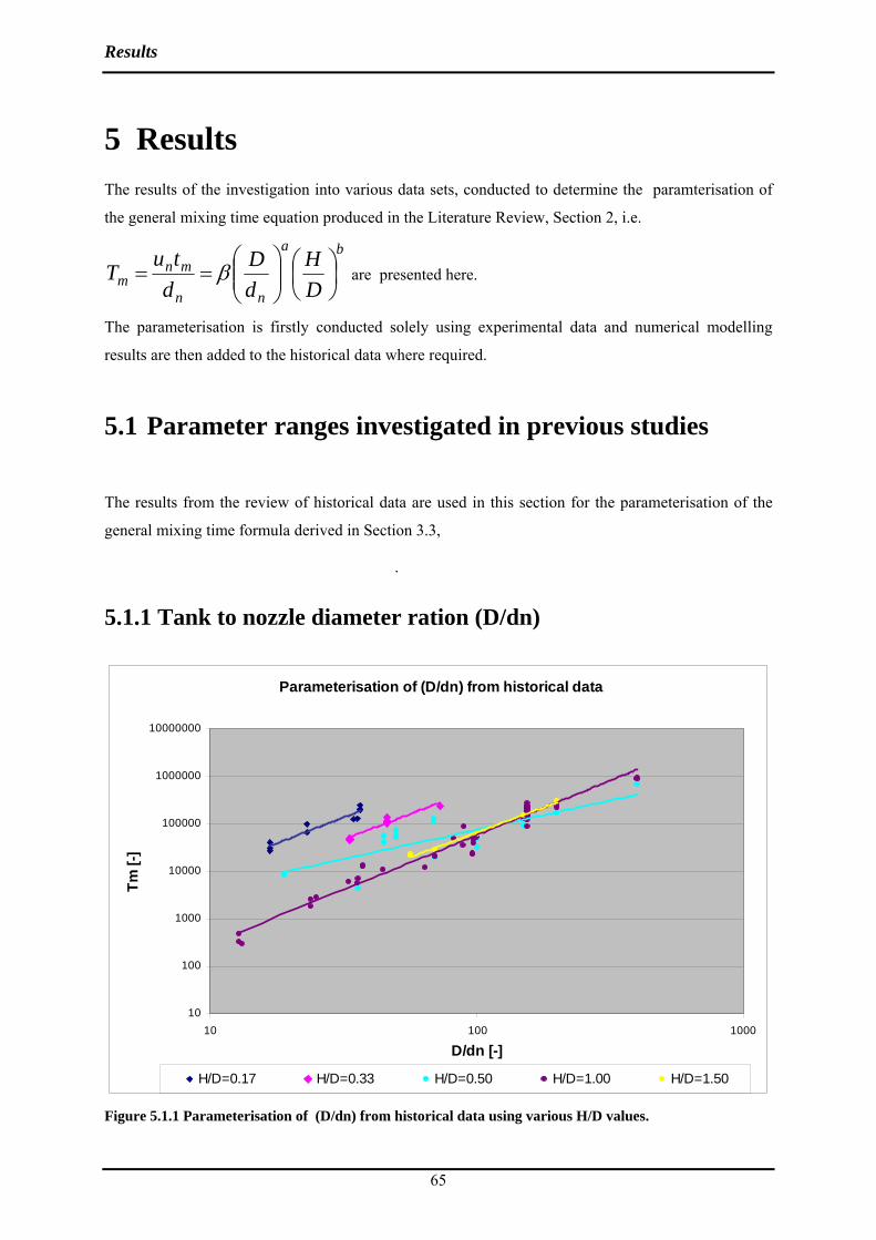
Results
65
5 Results The results of the investigation into various data sets, conducted to determine the paramterisation of
the general mixing time equation produced in the Literature Review, Section 2, i.e.
ba
nn
mnm D
HdD
dtuT ⎟
⎠⎞
⎜⎝⎛
⎟⎟⎠
⎞⎜⎜⎝
⎛== β are presented here.
The parameterisation is firstly conducted solely using experimental data and numerical modelling
results are then added to the historical data where required.
5.1 Parameter ranges investigated in previous studies
The results from the review of historical data are used in this section for the parameterisation of the
general mixing time formula derived in Section 3.3,
.
5.1.1 Tank to nozzle diameter ration (D/dn)
Parameterisation of (D/dn) from historical data
10
100
1000
10000
100000
1000000
10000000
10 100 1000
D/dn [-]
Tm [-
]
H/D=0.17 H/D=0.33 H/D=0.50 H/D=1.00 H/D=1.50
Figure 5.1.1 Parameterisation of (D/dn) from historical data using various H/D values.

Results
66
The details of the regressions fitted in Figure 5.1.1 are presented in Table 5.1.1 below.
Table 5.1.1 Summary details for regressions performed in Figure 5.1.1.
H/D Parameterisation of
D/dn Regression R2 value
0.17 2.2 0.9
0.33 2.1 0.9
0.50 1.2 0.7
1.00 2.3 1.0
1.50 2.1 1.0
Figure 5.1.1 indicates sufficient data for a critical analysis of the parameterisation of (D/dn) is only
available at H/D=0.5 and 1. For this reason, these data ranges are examined further via a breakdown of
the collated data into their literature sources in Figure 5.1.2 and Figure 5.1.4..
Parameterisation of (D/dn) from historical data - for H/D=0.5
Tm = 12.9(D/dn)2.1
R2 = 0.9
Tm = 2.8(D/dn)2.1
R2 = 1.0
10
100
1000
10000
100000
1000000
10000000
10 100 1000
D/dn [-]
Tm [-
]
Rossman and Grayman (1999) Okita and Oyama (1963)
Figure 5.1.2 5.1.3 Parameterisation of (D/dn) from historical data for H/D=0.5

Results
67
Parameterisation of (D/dn) from historical data - for H/D=1.0
Tm = 1.0(D/dn)2.4
R2 = 1.0
Tm = 3.6(D/dn)2.1
R2 = 1.0
Tm = 12.4(D/dn)1.7
R2 = 1.0
10
100
1000
10000
100000
1000000
10000000
10 100 1000
D/dn [-]
Tm [-
]
Zughbi and Rakib (2002) Zughbi and Rakib (2004) Patwardhan and Gaikwad (2003)Okita and Oyama (1963) Fox and Gex (1956)
Figure 5.1.4 Parameterisation of (D/dn) from historical data- were H/D =1.0
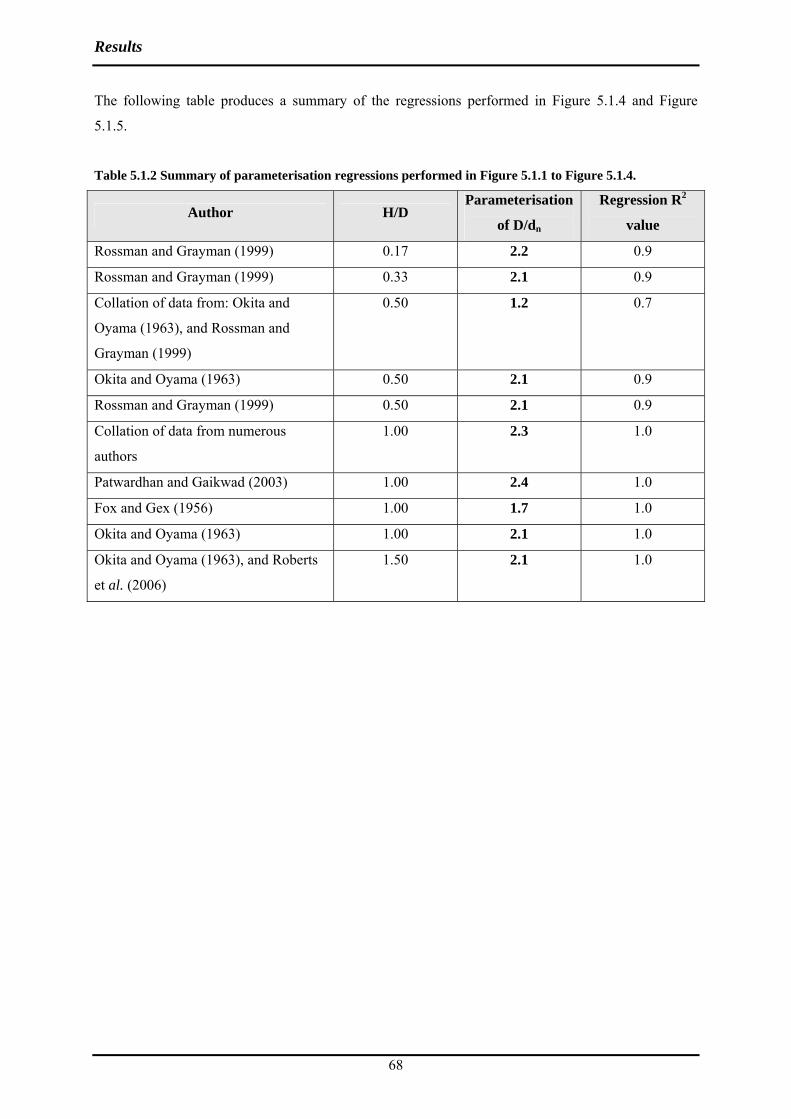
Results
68
The following table produces a summary of the regressions performed in Figure 5.1.4 and Figure
5.1.5.
Table 5.1.2 Summary of parameterisation regressions performed in Figure 5.1.1 to Figure 5.1.4.
Author H/D Parameterisation
of D/dn
Regression R2
value
Rossman and Grayman (1999) 0.17 2.2 0.9
Rossman and Grayman (1999) 0.33 2.1 0.9
Collation of data from: Okita and
Oyama (1963), and Rossman and
Grayman (1999)
0.50 1.2 0.7
Okita and Oyama (1963) 0.50 2.1 0.9
Rossman and Grayman (1999) 0.50 2.1 0.9
Collation of data from numerous
authors
1.00 2.3 1.0
Patwardhan and Gaikwad (2003) 1.00 2.4 1.0
Fox and Gex (1956) 1.00 1.7 1.0
Okita and Oyama (1963) 1.00 2.1 1.0
Okita and Oyama (1963), and Roberts
et al. (2006)
1.50 2.1 1.0

Results
69
5.1.2 Tank height to diameter ratio
Figure 5.1.5 shows the parameterisation of (H/D) from historical data for numerous values for (D/dn).
There was no overlap in testing for the different D/dn constants, thus the data for the parameterisation
of H/D is presented with their respective sources.
Parameterisation of (H/D) from historical data
100
1000
10000
100000
1000000
0.1 1.0 10.0
H/D [-]
Tm [-
]
D/dn=64.1, Okita and Oyama (1963) D/dn=46.0, Rossman and Grayman (1999)
D/dn=100.0, Okita and Oyama (1963) D/dn=150, Okita and Oyama (1963)D/dn=200, Okita and Oyama (1963)
Figure 5.1.5 Parameterisation of the H/D ratio using historical data only.

Results
70
A summary of the regressions performed in Figure 5.1.5, is detailed in Table 5.1.3.
Table 5.1.3 Summary details for regressions performed in Figure 5.1.5.
Author D/dn
Parameterisation of
H/D Regression R2 value
Okita and Oyama
(1963)
46 -0.8 0.7
Rossman and
Grayman (1999)
64 0.6 0.4
Okita and Oyama
(1963)
100 0.4 0.6
Okita and Oyama
(1963)
150 0.5 1.0
Okita and Oyama
(1963)
200 0.5 0.9
The H/D range investigated by previous studies that propose a mixing time formula and the value of
the parameterisation they suggest are presented in Figure 5.1.6, below.
Parameterisation of (H/D) with respect to the range of aspect ratios tested
0
0.5
1
1.5
2
2.5
3
3.5
0 0.5 1 1.5 2 2.5
H/D [-]
par
amet
eris
atio
n of
(H/D
) [-]
Fox and Gex 1956
Lane and Rice 1982
Okita and Oyama 1963
Maruyama et al. 1982
Grenville and Tilton 1997
Rossman and Grayman1999
Roberts et al. 2006
Simon and Fonade 1993
Coldrey 1978
Figure 5.1.6 Parameterisation of (H/D) with respect to the range of aspect ratios testing.
Results
71
5.2 CFD Modelling
It was determined from the analysis of results presented in Section 5.1 (analysis discussed in detail in
Section 6.2) that numerical results via CFD modelling were required to determine the parameterisation
of the H/D ratio. In this section, the numerical results derived from the present study are combined
with the historical data to allow for the parameterisation of the H/D ratio to be determined.
Figure 5.2.1 presents the separate regressions for the parameterisation of the H/D ratio, into their
experimental source and D/dn ratio. The numerical data is combined with the historical data for a
D/dn=100 to determine an alternate value for the parameterisation of the H/D ratio in Figure 5.2.2.
The numerical data is combined with the historical data for a D/dn=100, 150 and 200 to provide
another alternate value for the parameterisation of the H/D ratio in Figure 5.2.3. The parameterisation
of H/D is found to range between 0.4 and 1.0 in Figure 5.2.1, and is equal to 0.9 and 0.8 in the
regressions produced in Figure 5.2.2 and 5.2.3, respectively.

Results
72
Parameterisation of (H/D) from Numerical and Historical data
y = 184171.2x1.0
R2 = 1.0
Tm = 238869.3(H/D)0.5
R2 = 0.9 Tm = 126979.3(H/D)0.5
R2 = 1.0
Tm = 53435.8(H/D)0.4
R2 = 0.6
1000
10000
100000
1000000
0.1 1 10
H/D [-]
Tm [-
]
D/dn=100, Numerical results (present study) D/dn=100, Okita and Oyama (1963)D/dn=150, Okita and Oyama (1963) D/dn=200, Okita and Oyama (1963)
Figure 5.2.1 Parameterisation of H/D using numerical and historical data, over various D/dn ratios.

Results
73
Parameterisation of (H/D) from Numerical and Historical data - D/dn=100
Tm = 95976.3(H/D)0.9
R2 = 0.5
1
10
100
1000
10000
100000
1000000
0.1 1 10
H/D [-]
Tm [-
]
D/dn =100
Figure 5.2.2 Parameterisation of H/D ratio from collating numerical and historical data for D/dn=100.

Results
74
Parameterisation of (H/D) from Numerical and Historical data-D/dn~150
Tm = 137773.5(H/D)0.8
R2 = 0.3
1
10
100
1000
10000
100000
1000000
0.1 1 10
H/D [-]
Tm [-
]
D/dn =100,150,200
Figure 5.2.3 Parameterisation of H/D ratio by collating all historical and numerical data for D/dn=100,
150 and 200.
5.3 Constant, β
The constant, β, in the general mixing time formula is determined, after Sections 5.1 and 5.2 were
analysed to determine the parameterisation of the H/D and D/dn ratios. The parameterisation of H/D
and D/dn was estimated to be equal to 0.9 and 2.3 (as detailed in discussion provided in Sections
6.1and 6.2. Using the estimates derived from this analysis, the constant was determined via the various
regressions of numerical and historical data, presented below.
Figure 5.3.1, presents the regression derived from the numerical results only, while Figure 5.3.2
combines the historical and numerical data for a D/dn=100. Figure 5.3.3 combines all the historical
and numerical data for a D/dn=100, 150 and 200 to determine the value of the constant, β. The
constant, β is found to be equal to 7.9, 7.5 and 1.6, from the regressions produced in Figure 5.2.4,
5.2.5 and 5.2.6, respectively.

Results
75
Evaluation of constant in general mixing time formula- using numerical results only
Tm = 7.9x - 6579.6R2 = 1.0
0.00E+00
1.00E+05
2.00E+05
3.00E+05
4.00E+05
5.00E+05
6.00E+05
0 10000 20000 30000 40000 50000 60000 70000 80000
x= (D/dn)^2.2 (H/D)^0.9 [-]
Tm [
-]
D/dn=100
Figure 5.3.1 Evaluation of the constant using only the results of the numerical study.
Evaluation of constant in general mixing time formula- using numerical and historical data - D/dn=100
Tm = 7.5x - 65239.8R2 = 0.7
1
10
100
1000
10000
100000
1000000
1000 10000 100000
x= (D/dn)^2.2 (H/D)^0.9 [-]
Tm [-
]
D/dn=100, H/D=varied
Figure 5.3.2 Evaluation of the constant using numerical and historical results for a D/dn=100.

Results
Evaluation of constant in generalised mixing time formula - numerical and historical data - D/dn~150
Tm = 1.6x + 58860.5R2 = 0.4
1
10
100
1000
10000
100000
1000000
1000 10000 100000 1000000
x= (D/dn)^2.2 (H/D)^0.9 [-]
Tm [-
]
D/dn=100,150,200 and H/D=varied
Figure 5.3.3 Evaluation of the constant using numerical and historical results for a D/dn=100, 150 and
200.
76

Discussion
77
6 Discussion This section discusses the results presented in Section 5, and draws conclusions on the value of the
parameterisation constants, a and b, and experimental constant, β in the general mixing time equation,
ba
nm D
HdDT ⎟
⎠⎞
⎜⎝⎛
⎟⎟⎠
⎞⎜⎜⎝
⎛= β .
6.1 Tank and nozzle diameter ratio (D/dn)
Figure 5.1.1 shows that the tank to inlet diameter ratio, D/dn, has been tested over a wide range, from
20 to 400 when H/D is held constant. Most water storage tanks in operation in Western Australia have
tank to nozzle diameter ratios within this range (pers. comm. Thomas Ewing). The positive slope
coefficients in Figure 5.1.1 indicate that experimental evidence agrees well with jet theory, as detailed
in Section 3.3.3.1
It is observed that a set of parallel lines exists for H/D = 0.17, 0.25, 0.33 and 1.5. At H/D=0.5, a
significantly different slope with a very low correlation coefficient (R2≈0.5) is produced. Figure 5.1.2
breaks down the data for H/D=0.5 into the literature sources, and it is observed that the low correlation
observed in Figure 5.1.1 is due to the differing results produced by, Rossman and Grayman (1999) and
Okita and Oyama (1963). The difference in results is most attributable to the data scatter inherent in
both studies and the differences in experimental method. Maruyama et al. (1982), Lane and Rice
(1982) and Revill (1992) find a ±30 per cent data scatter in the Okita and Oyama (1963) study, while
Roberts et al. (2006) claim significant data scatter in the Rossman and Grayman (1999) study.
As detailed previously, Rossman and Grayman (1999) account for the differences between their results
and that produced by Okita and Oyama (1963) as being due to:
1. a more stringent definition for complete mixing was defined; and
2. the tracer was added with an external inflow instead of internal recirculation.
The effect of the definition for complete and tracer injection on the mixing times recorded is detailed
in Section 3.5.1 and 3.5.2.3, respectively. However, the present study finds that predicts that it is in
fact the significantly different inlet configurations employed by each of the studies. While Rossman
and Grayman (1999) employ near bottom horizontal and central, vertical feed inlet configurations,
Okita and Oyama (1963) employ inclined, side entry inlet configurations. Thus, the regression
produced from the combination of the Rossman and Grayman (1999) and Okita and Oyama (1963), is

Discussion
78
disregarded for the parameterisation of the D/dn ratio, as it is predicted to incorporate factors such as
the nozzle angle and location rather than the effect of the D/dn ratio with mixing time.
Figure 5.1.1 shows that the largest and widest data set exists for H/D =1, which is tested across the
across range of D/dn=20 – 400. The regression produced for H/D=1 in Figure 5.1.1, combines the data
of many authors (as shown in Figure 5.1.4) to produce a regression with a high R2 value of 0.9 and
suggests a parameterisation value of 2.3. It should be noted that the data set used to produce this
regression, comes from experiments which all employ inclined, side entry inlet configurations, most
likely accounting for the large R2 value.
When the data for H/D=1 is broken down to its literature sources it is apparent that the data is
predominantly derived from the works of Patwardhan and Gaikwad (2003) and Okita and Oyama
(1963), as presented in Figure 5.1.4. Both, Patwardhan and Gaikwad (2003) and Okita and Oyama
(1963) produce strong linear correlations with R2 values of approximately 1.0. Their parameterisation
values for the D/dn ratio are also similar, approximately equalling 2.4 and 2.1, respectively. However,
both works measured mixing time using probe measurement techniques, and neither located probes
with an understanding to the circulation patterns within their experimental tank configurations. The
inaccuracy in the employment of a probe measurement technique is detailed in Section 3.5.2. While
Patwardhan and Gaikwad (2003) used at least four measuring probes, Okita and Oyama (1963) only
used two.
Aside from the issue of probe measurement, and data scatter in the works of Okita and Oyama (1963),
the reliability of the results produced by Patwardhan and Gaikwad (2003) is also questionable. This is
because the experimental procedure used by Patwardhan and Gaikwad (2003) employs the Patwardhan
(2002) experimental method, which resulted in unexplained asymmetry of flow. The experimental set
up of Patwardhan (2002) is shown in Figure 6.1.1, where the conductivity measuring probes are placed
at locations 1 to 4. As indicated in Figure 6.1.1, the tracer was injected at the centre of the top liquid
surface. From the indicated tank configuration it is expected that the measured concentration profiles
at locations 1 and 4 should be identical, however this is not the case as indicated by Patwardhan
(2002)’s results in Figure 6.1.2. Patwardhan (2002) also notes the unexpected significant difference
between the findings of probe 1 and 4, however does not investigate or explain the finding further, and
instead ignores the findings and carries out the remaining work under the assumption that the probes 1
and 4 do produce identical results.

Discussion
79
Figure 6.1.1 Experimental Set-up of Patwardhan (2002).
Figure 6.1.2 Normalised concentration profiles at each probe from physical scale modelling experiments
performed by Patwardhan (2002).
6.1.1 Summary
The tank to inlet diameter has been tested over a sufficiently wide range, with respect to typical tank
configurations in Western Australia (pers. comm. Thomas Ewing). Table 5.1.2 summarises the
parameterisation values derived from the various regressions performed in Section 5.1.1. Table 5.1.2
indicates that despite the significant data error in the works of Okita and Oyama (1963) and Rossman
and Grayman (1999), as well as the concern for possible experimental error in the works of
Patwardhan and Gaikwad (2003), they all are in agreement that the parameterisation of the D/dn ratio
lies within the narrow range of 2.1-2.4. This agreement in the historical data and the measurement of
D/dn over a large experimental range, suggests that the best estimate for the parameterisation of D/dn is
2.3. The parameterisation value of 2.3 is chosen as the best estimate because: it is derived from the
combined data set of various, independent, studies; produces a high R2 value of 0.9; and lies within the
narrow experimental result range of 2.1-2.4.
Discussion
80
6.2 Tank height to diameter ratio (H/D)
The results of the investigation into the parameterisation of the H/D ratio are discussed here by firstly
focusing on the results of historical data and then extending the examination to the influence of the
numerical data.
6.2.1 Historical results and data
Figure 5.1.5 shows that the dimensionless parameter, H/D, has been tested only over a limited range of
approximately 0.25-1.5, when D/dn is held constant. Figure 5.1.5 indicates that Okita and Oyama
(1963) are the only authors to test H/D over a given range in a consistent manner. Table 5.1.3 indicates
that when H/D = 150 and 200, high correlation coefficients are produced (R2=0.1 and 0.9,
respectively) indicating that the parameterisation of H/D is approximately equal to 0.5.
Positive, low, correlation coefficients are produced for D/dn = 64.1 and 100, and a negative, low,
correlation coefficient is produced for D/dn = 46.0. The reasoning behind a weak correlation at D/dn
=100, and strong correlations at D/dn =150 and 200, by Okita and Oyama (1963) is unclear. The low
correlation coefficient for D/dn= 64.1, is attributable to the employment of a purely visual measuring
technique by Fox and Gex (1956) and the inaccuracy inherent in such experimental techniques. The
negative, weak, correlation coefficient derived by Rossman and Grayman (1999) for =46.0, is most
likely attributable to their employment of two drastically different inlet configurations. They vary the
inlet angle and location from a horizontal, side jet at H/D=0.22, to a vertical jet located at the centre of
the tank bottom at H/D=0.33, thereby providing possible explanation for the low correlation
coefficient (R2=0.1) derived for D/dn = 46.0. It should be noted that although Okita and Oyama (1963)
also vary jet angle, they do not vary jet location, providing possible explanation for why the effects of
nozzle angle and location are not as prominent in their results as it is on the results of Rossman and
Grayman (1999).
Figure 5.1.6 further highlights the limited testing of the dimensionless tank geometry parameter, H/D,
in the derivation of many of the existing mixing time formulae. As Figure 5.1.6 shows both the mixing
time formulae derived by Coldrey (1978) and Simon and Fonade (1993) has only been tested over the
particular value of H/D=1. Both these authors derive their mixing time formulae, essentially by a
process of empirical derivation, thus indicating that their respective mixing time formulae are only
Discussion
81
applicable at the most to H/D=1. Figure 5.1.6 also shows that there has been limited testing at values
greater than H/D=1.
6.2.1.1 Summary
Therefore, Okita and Oyama (1963) are the only authors to test the effects of tank geometry in a
consistent manner. Furthermore the existing formulae have only been validated against a very narrow
H/D range. The testing of the dimensionless parameter H/D has also been limited to a small range (0.5
to 1.5), and more testing is required both within and outside the given range tested by previous studies.
As discussed in Section 4, for these reasons, CFD modelling is employed in the present study to
provide another, more reliable data source for comparison with the Okita and Oyama (1963) study and
ultimately the parameterisation of the H/D ratio. The following, Section 6.2.2, discusses the CFD
modelling results for the parameterisation of the H/D ratio.
6.2.2 CFD modelling
As shown in Figure 5.2.1, the CFD modelling results indicate, likewise to the previous study of Okita
and Oyama (1963), that a strong, positive, linear relationship exists, between H/D and the
dimensionless mixing time, Tm. This linear relationship indicates that the parameterisation of the H/D
ratio is of constant value under the given range tested (i.e H/D=0.3-3). The regression produced for the
numerical results indicate that this constant value for the parameterisation of the H/D ratio, under the
given range tested, is approximately equal to 1.
Figure 5.2.1, compares the CFD modelling results with the historical data. It is evident in Figure 5.2.1,
that the parameterisation value derived by the CFD modelling work of the present study (=1), is
significantly different to that derived historically by Okita and Oyama (1963) (≈0.5). When the
numerical data is combined with the data from Okita and Oyama (1963) for D/dn=100, there is a
minimal change in the value of the parameterisation constant, at 0.9 in Figure 5.2.2. Similarly even for
the large data base that includes all data points for D/dn=100,150 and 200, there is only a slight change
in the parameterisation constant, at a value of 0.8, in Figure 5.2.3.
A major discrepancy in the existing work that was only discovered during the CFD modelling stage, is
the inaccurate capture of mixing time, by the method of mixing time evaluation employed. This
discovery has never been reported before in the literature survey and due to the significance to mixing

Discussion
82
time measurement is discussed in detail in Section 4.2.5.1. The error occurs due to the capture of the
jet in the mixing time evaluation, which causes the recorded mixing time to potentially be
overestimated.
6.2.3 Summary
As detailed previously, the work of Okita and Oyama (1963) has been found by later studies to have a
±30% data error. There is also error inherent in the calculation of mixing time in the present CFD
modelling work, as detailed in previous section, where the derived mixing times are potentially
overestimated. Even though data error is apparent in both these independent studies, Okita and Oyama
(1963) and the present study, there is little change in the H/D parameterisation constant (from Figures
5.2.1 to 5.2.3). Further the data error in both these studies are separate to each other i.e. the error in the
numerical work is not the same type of error being recorded in the physical scale modelling work of
Okita and Oyama (1963). It is thus, concluded that a parameterisation constant can be estimated with
confidence from the data output. The best estimate for the parameterisation of the H/D parameter is
chosen to be equal to 0.9, as derived by the regression in Figure 5.2.2. This is because in Figure 5.2.2
the parameterisation constant is determined from a larger data set than in Figure 5.2.1, and deviates
only very slightly from the parameterisation constant estimated in Figure 5.2.1 (where b=1.00).
6.3 Constant, β
The constant β, is determined after, the parameterisation values for D/dn and H/D are determined. The
regressions indicating the value of the constant for different data set combinations is provided in
Figures 5.2.4 to 5.4.6. Similarly to the parameterisation of the H/D ratio, there is little difference to the
constant produced by regressions using the numerical data set only compared to that combining with
the experimental data of Okita and Oyama (1963). Figure 5.2.4 and 5.2.5 produce a β value of 7.9 and
7.5 , respectively, while the combination of all available data in Figure 5.2.6 produces a β value of 1.6.
Thus, the constant, β is estimated to lie between 7.5 and 7.9, due to their close agreement in value,
rather than 1.6. The best estimate is determined as 7.5, so as to maintain consistency with the method
employed in Section 6.1.2, where the data set combining Okita and Oyama (1963) and the numerical
study was chosen as providing the best estimate for the parameterisation constant of the H/D ratio (i.e.
b). Table 6.1.1 compares the constant value derived in the present study with that from the mixing
time formula of previous studies of similar form. In Table 6.1, it is observed that the constant chosen

Discussion
as the best estimate of β in the present study, lies within the range of that derived by Okita and Oyama
(1963) and Rossman and Grayman (1999).
Table 6.3.1 Comparison of the value of the constant in the mixing time formula, derived by various
studies.
Author Proposed constant, β, value
Okita and Oyama (1963) 5.5
Rossman and Grayman (1999) 9.8
Present study 7.7
6.4 Summary
With the collation and analysis of historical and numerical data the following mixing time equation is
derived by the present study.
ba
nm D
HdDT ⎟
⎠⎞
⎜⎝⎛
⎟⎟⎠
⎞⎜⎜⎝
⎛= β 6.4.1
Where: a = 2.3,
b = 0.9,
β = 7.5.
Although, there is error in the measurement technique employed to derive the numerical data and
errors are reported in the historical data, the collectively produce very similar results. Furthermore,
high correlation coefficients are produced for majority of the regressions used to investigate the
parameterisation of D/dn and H/D. No other study surveyed in the existing literature has derived the
parameterisation of the D/dn and H/D ratios, over parameter ranges as large as that employed by the
present study. Further supporting the reliability of the parameterisation constants estimated.
83


Conclusions
85
7 Conclusions
The present study clarifies confined jet principles and highlights exactly where confined jet flow
dynamics deviates from free jet theory, and how this affects the mixing characteristics in a tank.
Mixing characteristics within tank systems fitted with jet mixers, are governed by the turbulent mixing
process that occurs when ambient tank fluid is entrained into the jet. In a turbulent situation where
there are no density differences, pure jet fundamentals indicate that the rate of mixing is a function of
entrainment only. The entrainment rate for an unconfined (free) jet is a function of the distance from
the source and the initial jet momentum. In comparison to unconfined jet cases, under confined jet
situations, mixing is still a function of entrainment, however the interaction of the jet with the
boundaries alters the rate of entrainment. This confined jet entrainment rate can not be clearly defined
under the present state of knowledge due to the inability to quantify; the cessation of entrainment
when jet attachment of boundary exists, the frictional forces that come into play when such an event
occurs, and the effect of different circulation patterns caused by various tank configurations.
The mixing time formulae produced by previous studies into jet mixing employ either free jet theory
or empirical means for their formula derivation. The method of formula derivation employed by
previous studies is not supported by the present study, as application of free jet theory to confined jet
situations is not correct for reasons outlined in the discussion earlier, and the empirical derivation of a
formula has no physical basis. Furthermore, the existing mixing time formulae have been
parameterised using data from a very narrow range of H/D ratios, limiting their robustness to different
tank geometries.

Conclusions
86
This study finds the mixing time formula for jet mixing within tanks to be ,
9.03.2
5.7 ⎟⎠⎞
⎜⎝⎛
⎟⎟⎠
⎞⎜⎜⎝
⎛=
DH
dDT
nm 7.0.1
Where: n
mnm d
tuT = .
Equation 7.0.1 is applicable under the following conditions:
o 20< D/dn <200;
o 0.3< H/D <3;
o the tank is cylindrical in shape, with a flat-bottom;
o inlet nozzle has a circular cross-section; and
o ambient fluid is completely mixed and stationary.
The proposed mixing time formula (Equation 7.0.1) has a greater degree of validity to previously
proposed formulae because it is derived from data which span a significantly larger range of
parameters than any other existing formulae investigated. Further and more importantly, the formula is
derived from the collation and critical review of jet principles, historical data and numerical data.
The effect of inlet nozzle angle and location was found to have an effect on mixing time, however the
effect was secondary to the effects of the dimensionless ratios, H/D and D/dn. Existing formulae
attempt to capture the degree of jet interaction with the free jet path length, L, parameter. The present
work finds that upon critical review of existing experimental evidence and application of jet theory
principles, parameter L is unable to capture and predict the effects of various inlet configurations on
mixing time. This is because the effect of nozzle angle and location is a function of many parameters
such as: L, proximity to boundaries, interaction with boundaries, velocity of circulatory flows and
circulatory flow patterns. Thus, parameter L is too simplistic to capture effects of various inlet
configurations. Experimental evidence also suggests at higher jet inflow rates, the difference in mixing
times between various tank configurations is reduced.
Conclusions
87
In regard to the measurement and evaluation of mixing time, the present study has drawn some
important conclusions on the validity and limitations of different experimental methods. The major
limitation in probe measurement studies is the inability of the probe to capture the entire flow field,
and the concern that for this reason mixing time can be over or under estimated. While numerical
modelling with the use of CFD models has received much support in the literature, the present study
finds that the potential to overestimate mixing time due to the evaluation of the inflow jet in the
mixing time criterion, has not been reported in previous jet mixing studies. Similarly it was found that
although the LIF experimental method provides a physical scale modelling method which can capture
the entire flow field, care needs to be taken to ensure that the scanning planes capture the increase in
water height for the fill-and-draw tank operation model. Otherwise, mixing time is underestimated, as
was found to be the case with the work of Roberts et al. (2006).

Recommendations for Further Research
89
8 Recommendations for Further Research
Essentially, most practical applications of jet mixing involves the presence of buoyant flows, where
pure jet dynamics govern the mixing process and the buoyant jet dynamics govern the stratification
process in the tank (Ivey, 2006). Ideally future research should head in the direction to where a mixing
time formula that takes into account various inlet configurations and is applicable to buoyant jet
situations is produced. Before neutrally buoyant situations are complicated with the presence of
buoyant conditions, the effects of nozzle angle and location, need to be understood, and thus should be
the focus of future works. The current data base on the effect of inlet configuration on mixing time is
very small. Upon the production of a mixing time formula, that is able to capture the effect of inlet
configurations, the study into mixing in confined jets can be extended and employed in the studies of
confined buoyant jet dynamics.
Further experimental investigations should be carried out under the guidelines produced in the present
work. These guidelines are detailed below.
1. For cases where probe measurement is used:
a. Probes need to be placed in; low, medium and high mixing zones, to maximize
understanding of the tank scale mixing nature. These zones can be identified prior to
probe placement via the use of visual dye techniques.
b. A balance, between the number of probes needed to capture the flow field more
accurately, while not altering the flow characteristics of the tank due to their intrusive
nature needs to also be met.
2. For cases where CFD modeling is employed:
a. The possible overestimation via jet inclusion on the evaluation plane needs to be
incorporated into the analysis of results, when the mixing criterion is defined by a
minimal COV value.
b. Other methods of mixing time evaluation, such as the use of water age measurement,
should be investigated to minimize the data bias from jet inclusion on the evaluation
plane.
3. For cases where LIF method is employed:
a. Similarly, to CFD modeling, the possible overestimation via jet inclusion on the
evaluation plane needs to be incorporated in the analysis of results, when the mixing
criterion is defined by a minimal COV value.
b. The scanning planes need to increase with height of the fluid, so that the whole flow
field is in fact captured

Recommendations for Further Research
90
4. Tracer injection time should be minimized
5. Ideally tracer should be injected into the inflow so as to observe the direct mixing nature of
the jet with the ambient fluid and to avoid experimental bias due to injection location.

References
91
9 References BROOKER, L. (1993) Mixing with the jet set. Chemical Engineer, 16.
DAKSHINAMOORTHY, D., KHOPKAR, A. R., LOUVAR, J. F. & RANADE, V. V. (2006) CFD
simulation of shortstopping runaway reactions in vessels agitated with impeller and jets.
Journal of Loss Prevention in the Process Industries, 19, 570-581.
DONALD, M. B. & SINGER, H. (1959) Entrainment in turbulent fluid jets. Transactions of the
Institution of Chemical Engineers, 37, 255-264.
FOSSETT, H. (1951) The action of free jets in mixing of fluids. Transactions of the Institution of
Chemical Engineers, 29 322-332.
FISCHER, H., LIST, J., KOH, R., IMBERGER, J. & BROOKS, N. (1979) Mixing in Inland and
Coastal Waters, London, Academic Press.
GRAYMAN, W., ROSSMAN, L., CLIFFORD, A., DEININGER, A., SMITH, C., SMITH, F. &
SCHNIPKE, R. (2000) Water quality modeling of distribution system storage facilities.,
Denver, AWWA Research Foundation.
GRAYMAN, W., ROSSMAN, L., R, D. & C, S. (2004) Mixing and aging of water in distribution
system storage facilities. American Water Works Association Journal, 96, 70-80.
GRENVILLE, R. K. & TILTON, J. N. (1996) A new theory improves the correlation of blend time
data from turbulent jet mixed vessels. Chemical Engineering Research and Design, 74, 390-
396.
IVEY, G. (2006) Lecture notes, as distributed in ENIVRONMENTAL FLUID MECHANICS.
University of Western Australia
JAYANTI, S. (2001) Hydrodynamics of jet mixing in vessels. Chemical Engineering Science, 56,
193-210.
LANE, A. G. C. & RICE, P. (1982) An investigation of liquid jet mixing employing an inclined side
entry jet. Chemical Engineering Research and Design, 60, 171-176.
LEHRER, I. H. (1981) A new model for free turbulent jets of miscible fluids of different density and a
jet mixing time criterion. Chemical Engineering Research and Design, 59a, 247-252.
LIST, E. J. (1982) Turbulent jets and plumes. Annual Review of Fluid Mechanics, 14, 189-212.
MARTINSON, D. B. & LUCEY, A. D. (2004) Reduction of Mixing in Jet-Fed Water Storage Tanks.
Journal of Hydraulic Engineering, 130, 75-81.
MARUYAMA, T., BAN, Y. & MIZUSHINA, T. (1982) Jet mixing of fluids in tanks. Journal of
Chemical Engineering of Japan, 15, 342-348.
NORDBLOM, O. & BERGDAHL, L. (2004) Initiation of Stagnation in Drinking Water Storage
Tanks. Journal of Hydraulic Engineering, 130, 49-57.

References
92
ORFANIOTIS, A., FONADE, C., LALANE, M. & DOUBROVINE, N. (1996) Experimental Study of
the Fluidic Mixing in a Cylindrical Reactor. The Canadian Journal of Chemical Engineering,
74, 203-212.
PATWARDHAN, A. W. (2002) CFD modeling of jet mixed tanks. Chemical Engineering Science, 57,
1307-1318.
PATWARDHAN, A. W. & GAIKWAD, S. G. (2003) Mixing in tanks agitated by jets. Transactions
of the Institution of Chemical Engineers, 81, 211-220.
PATWARDHAN, A. W., PANDIT, A. B. & JOSHI, J. B. (2003) The role of convection and turbulent
dispersion in blending. Chemical Engineering Science, 58, 2951-2962.
RAJARATNAM, N. (1976) Turbulent Jets, New York, Elsevier Scientific Publishing Company.
REVILL, B. K. (1992) Jet mixing. Mixing in the Process Industries. 2nd ed. Oxford, Butterworth-
Heinemann Ltd. .
ROBERTS, P. J. W., TIAN, X., LEE, S., SOTIROPOULOS, F. & DUER, M. (2006) Mixing in
storage tanks - draft final report. AWWA Research Foundation.
ROSSMAN, L. A. & GRAYMAN, W. M. (1999) Scale-model studies of mixing in drinking water
storage tanks. Journal of Environmental Engineering, 125, 755-761.
SIMON, M. & FONADE, C. (1993) Experimental study of mixing performances using steady and
unsteady jets. Canadian Journal of Chemical Engineering, 507-513.
WASEWAR, K. (2006) A Design of Jet Mixed Tank. Chemical Biochemical Engineering, 20, 31-46.
ZUGHBI, H. D. & RAKIB, M. A. (2002) Investigations of mixing in a fluid jet agitated tank.
Chemical Engineering Communications, 189, 1038-1056.
ZUGHBI, M. A. & RAKIB, H. D. (2004) Mixing in a fluid jet agitated tank: effect of jet angle and
elevation and number of jets. Chemical Engineering Science, 59, 829-842.

Appendix
93
10 Appendix
10.1 CFD Validation Data Experimental Setup
Figure 10.1.1 Experimental Setup of Roberts et al. (2006).
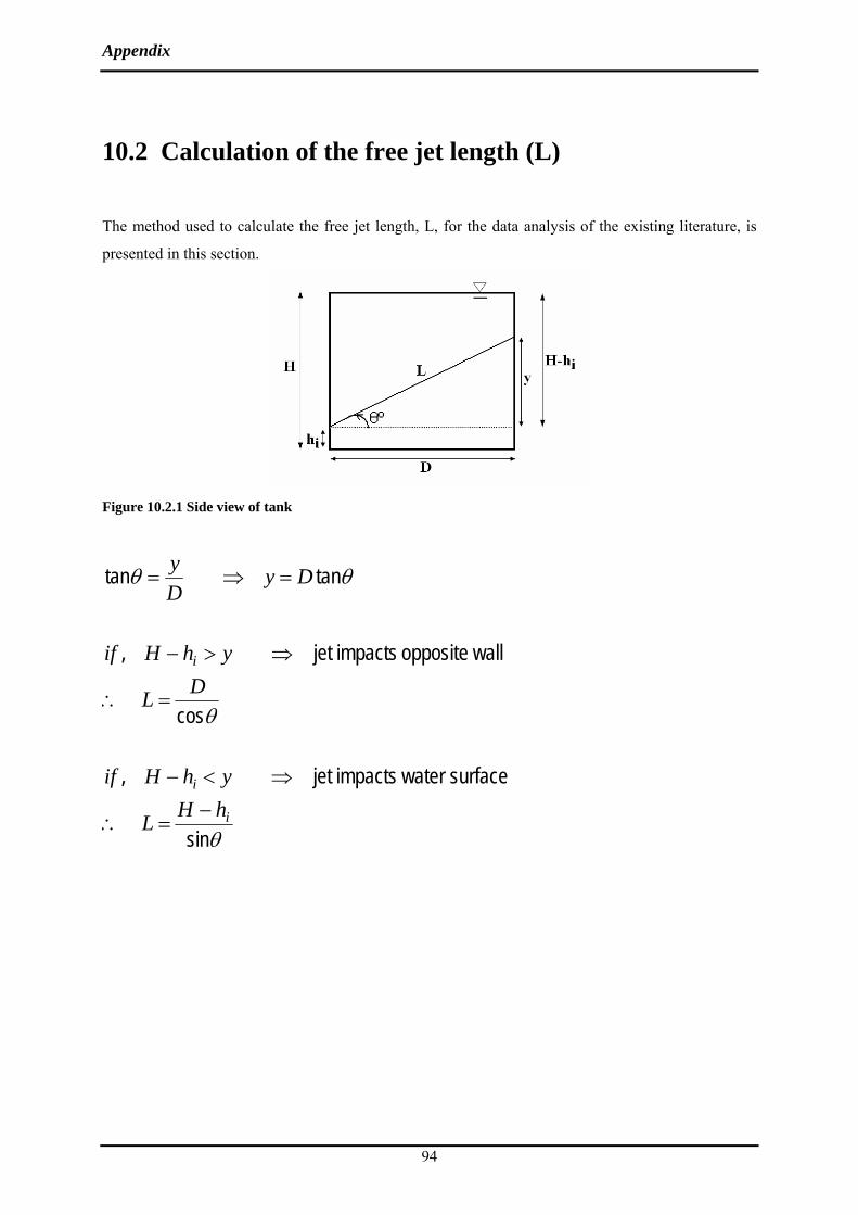
Appendix
94
10.2 Calculation of the free jet length (L)
The method used to calculate the free jet length, L, for the data analysis of the existing literature, is
presented in this section.
Figure 10.2.1 Side view of tank
θ
θ
θθ
sin
surface waterimpactsjet ,
cos
wallopposite impactsjet ,
tantan
i
i
i
hHL
yhHif
DL
yhHif
DyDy
−=∴
⇒<−
=∴
⇒>−
=⇒=

Appendix
10.3 Meshing details
Figure 10.3.1 Side view of the plane of symmetry for the grid used in CFD modelling stage
Figure 10.3.2 View of tank centred on z-axis used in CFD modelling stage
95