moving boundaries in earthscapes damien t. kawakami, v.r. voller, c. paola, g. parker, j. b. swenson...
Post on 20-Dec-2015
214 views
TRANSCRIPT
Moving Boundaries in Earthscapes
Damien T. Kawakami, V.R. Voller, C. Paola, G. Parker, J. B. Swenson
NSF-STC
www.nced.umn.edu
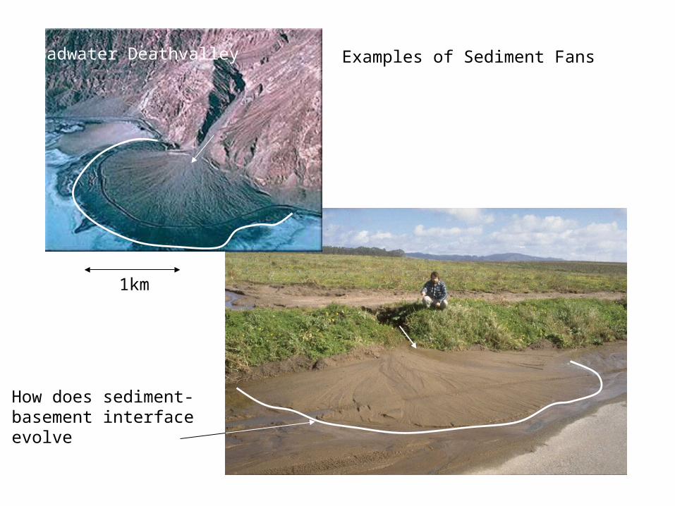
1km
Examples of Sediment Fans
How does sediment-basement interfaceevolve
Badwater Deathvalley
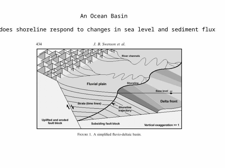
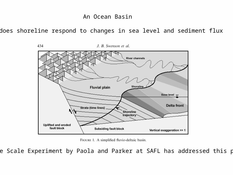
An Ocean Basin
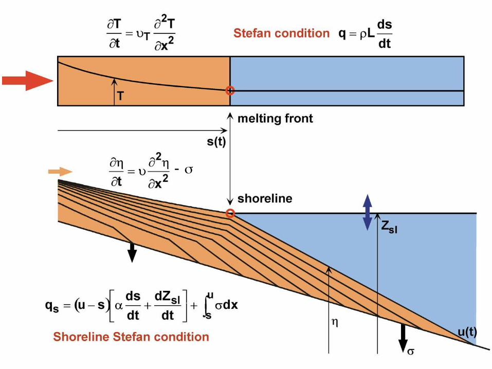
How does shoreline respond to changes in sea level and sediment flux
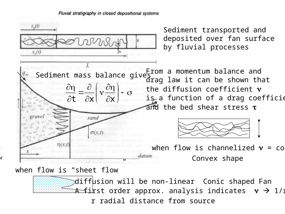
Sediment mass balance gives
Sediment transported and deposited over fan surfaceby fluvial processes
xxt
From a momentum balance anddrag law it can be shown thatthe diffusion coefficient is a function of a drag coefficientand the bed shear stress
when flow is channelized = cont.
when flow is “sheet flow”
diffusion will be non-linear Conic shaped Fan A first order approx. analysis indicates 1/r r radial distance from source
Convex shape
An Ocean Basin
How does shoreline respond to changes in sea level and sediment flux
A large Scale Experiment by Paola and Parker at SAFL has addressed this problem
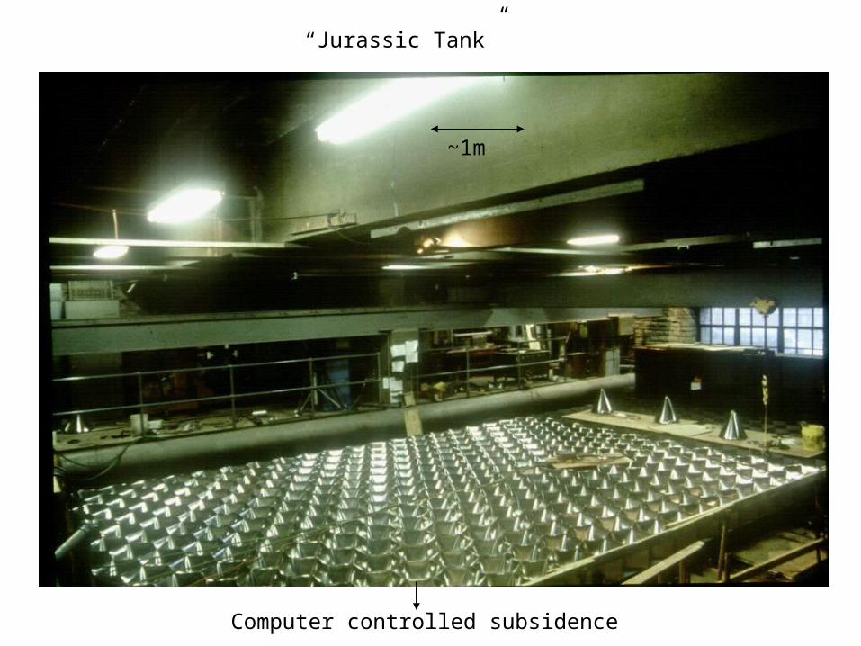
“Jurassic Tank”
~1m
Computer controlled subsidence
xxt
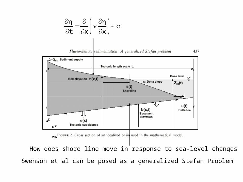
How does shore line move in response to sea-level changes
Swenson et al can be posed as a generalized Stefan Problem
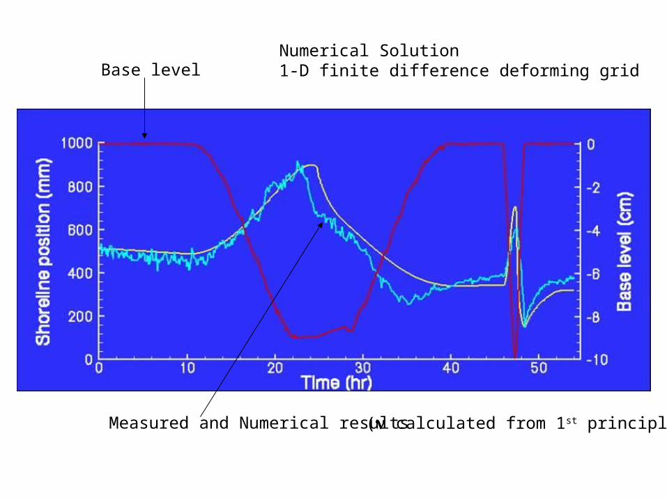
Base level
Measured and Numerical results ( calculated from 1st principles)
Numerical Solution1-D finite difference deforming grid
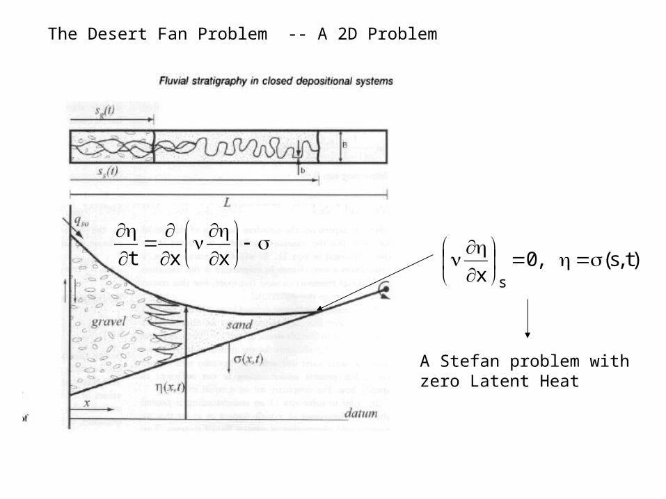
The Desert Fan Problem -- A 2D Problem
xxt )t,s(,0x s
A Stefan problem with zero Latent Heat
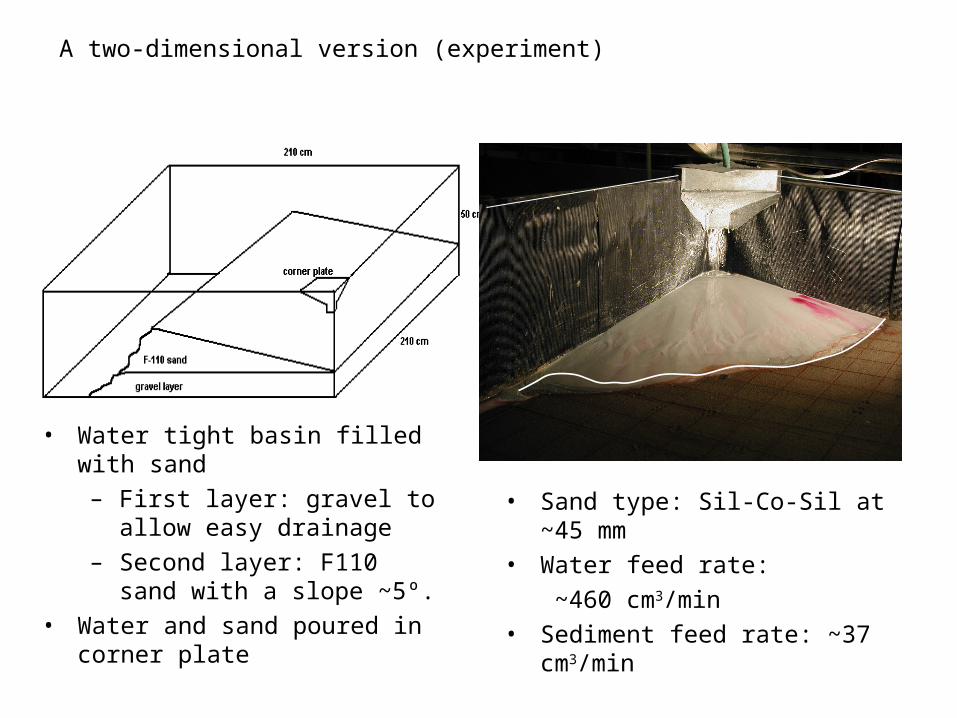
A two-dimensional version (experiment)
• Water tight basin filled with sand– First layer: gravel to allow
easy drainage– Second layer: F110 sand
with a slope ~5º.• Water and sand poured in
corner plate
• Sand type: Sil-Co-Sil at ~45 mm
• Water feed rate: ~460 cm3/min
• Sediment feed rate: ~37 cm3/min
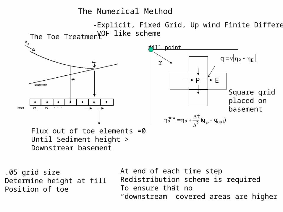
The Numerical Method
-Explicit, Fixed Grid, Up wind Finite Difference VOF like scheme
Flux out of toe elements =0Until Sediment height >Downstream basement
fill point
P
)qq(t
out2PnewP in
E
The Toe Treatment
EPq
Square grid placed onbasement
At end of each time stepRedistribution scheme is requiredTo ensure that no “downstream” covered areas are higher
r
.05 grid sizeDetermine height at fillPosition of toe
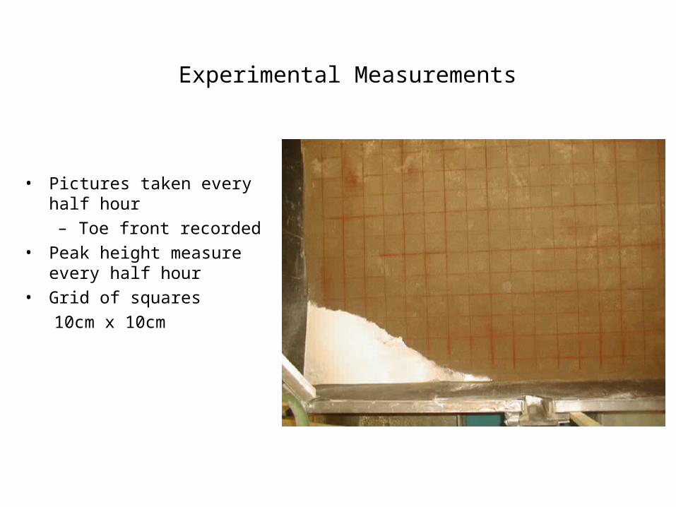
• Pictures taken every half hour– Toe front recorded
• Peak height measure every half hour
• Grid of squares 10cm x 10cm
Experimental Measurements
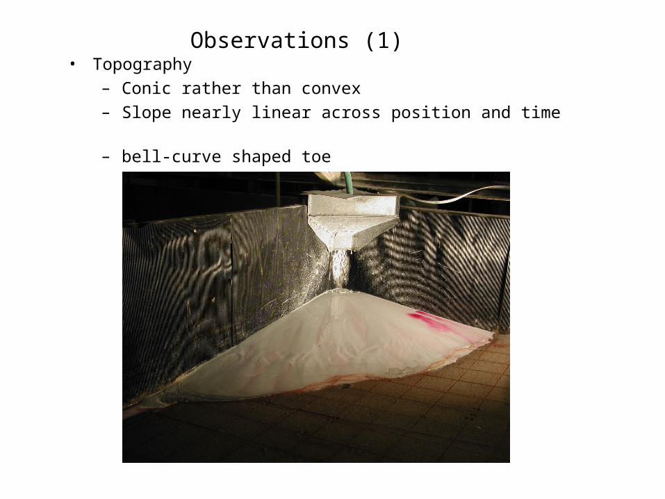
Observations (1)• Topography
– Conic rather than convex– Slope nearly linear across position and time – bell-curve shaped toe
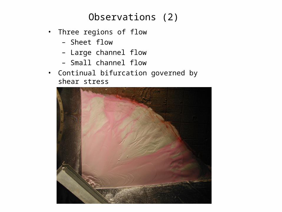
Observations (2)
• Three regions of flow– Sheet flow– Large channel flow– Small channel flow
• Continual bifurcation governed by shear stress
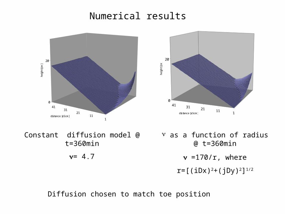
Numerical results
Constant diffusion model @ t=360min
= 4.7
as a function of radius @ t=360min
=170/r, where
r=[(iDx)2+(jDy)2]1/2
111213141
0
20
heig
ht [c
m]
distance [x5cm]
111
2131
41
0
20
heig
ht [c
m]
distance [x5cm]
Diffusion chosen to match toe position
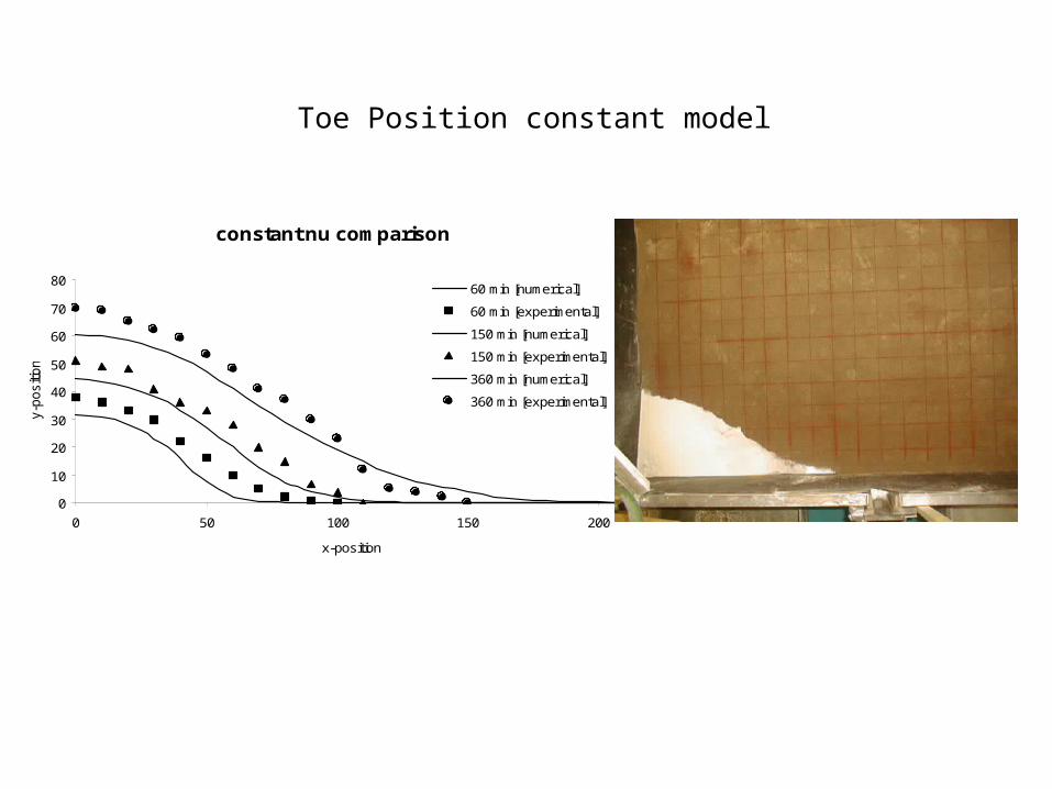
constant nu comparison
0
10
20
30
40
50
60
70
80
0 50 100 150 200
x-position
y-p
ositi
on
60 min [numerical]
60 min [experimental]
150 min [numerical]
150 min [experimental]
360 min [numerical]
360 min [experimental]
Toe Position constant model
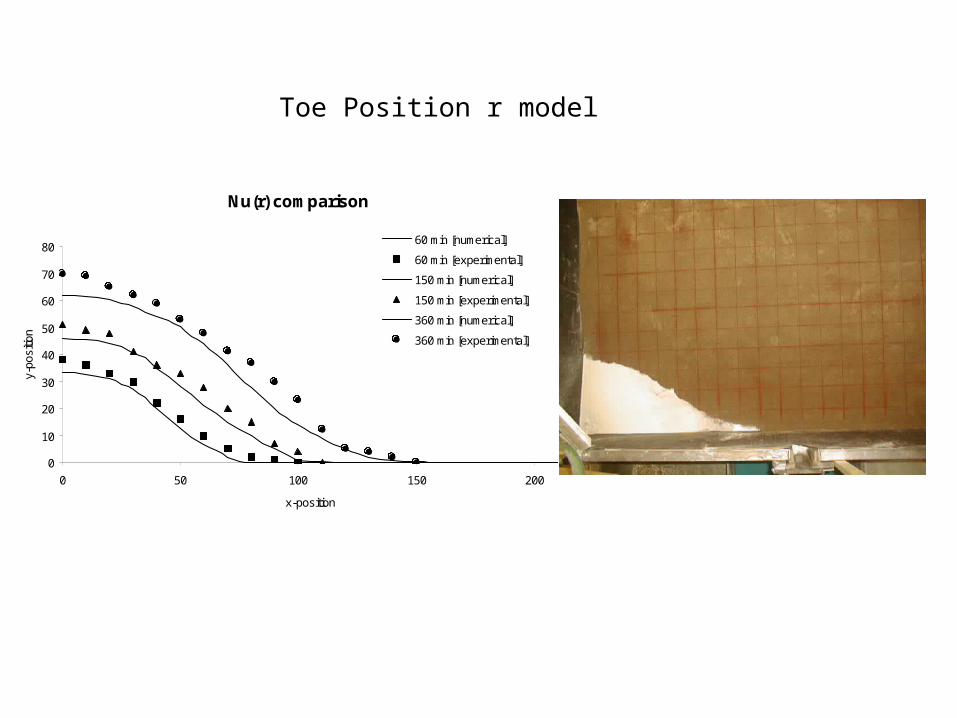
Nu(r) comparison
0
10
20
30
40
50
60
70
80
0 50 100 150 200
x-position
y-po
sitio
n
60 min [numerical]
60 min [experimental]
150 min [numerical]
150 min [experimental]
360 min [numerical]
360 min [experimental]
Toe Position r model
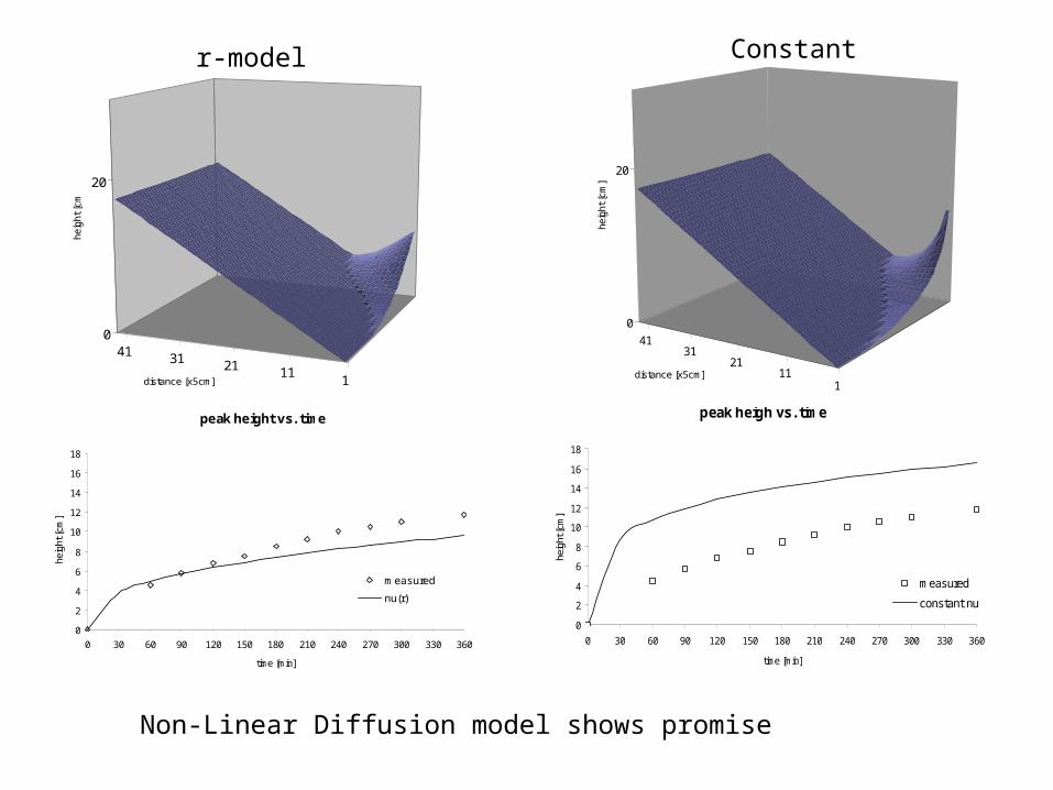
peak heigh vs. time
0
2
4
6
8
10
12
14
16
18
0 30 60 90 120 150 180 210 240 270 300 330 360
time [min]
heig
ht [c
m]
measured
constant nu
peak height vs. time
0
2
4
6
8
10
12
14
16
18
0 30 60 90 120 150 180 210 240 270 300 330 360
time [min]
heig
ht [c
m]
measured
nu(r)
111
2131
41
0
20
heig
ht [c
m]
distance [x5cm]111213141
0
20
heig
ht [c
m]
distance [x5cm]
Constantr-model
Non-Linear Diffusion model shows promise
Moving Boundaries in Earthscapes
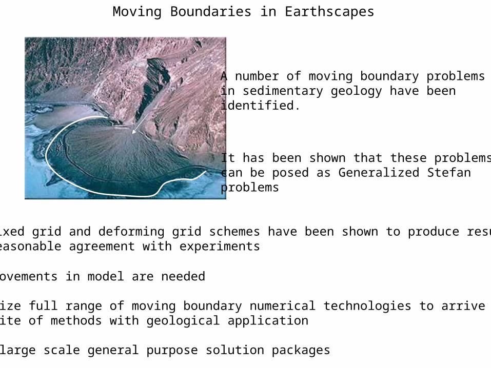
A number of moving boundary problems in sedimentary geology have beenidentified.
It has been shown that these problems can be posed as Generalized Stefan problems
Fixed grid and deforming grid schemes have been shown to produce results inReasonable agreement with experiments
Improvements in model are needed
Utilize full range of moving boundary numerical technologies to arrive at a suite of methods with geological application
Use large scale general purpose solution packages