mtm report 13 and cawrpt 2321 mtm broad-scale …€¦ · published by the manaaki taha moana (mtm)...

Ecological Survey of Tauranga Harbour

MTM Report No.13May 2013

ECOLOGICAL SURVEY OF TAURANGA HARBOUR

JOANNE ELLIS1, DANA CLARK1, JUDI HEWITT2, CAINE TAIAPA3, JIM SINNER1, MURRAY PATTERSON4, DERRYLEA HARDY4, STEPHEN PARK5, BRUCE GARDNER5, ALICE MORRISON5, DAVID CULLIFORD5, CHRIS BATTERSHILL6, NICOLE HANCOCK6, LYDIA HALE3, ROD ASHER1, FIONA GOWER1, ERIN BROWN7, AARON MCCALLION7 1CAWTHRON INSTITUTE, 2NIWA, 3MANAAKI TE AWANUI, 4MASSEY UNIVERSITY, 5BAY OF PLENTY REGIONAL COUNCIL, 6UNIVERSITY OF WAIKATO, 7WAKA DIGITAL

ISSN 2230-3332 (Print) ISSN 2230-3340 (Online) ISBN 978-0-9876639-2-4 Published by the Manaaki Taha Moana (MTM) Research Team Funded by the Ministry for Science and Innovation Contract MAUX0907 Main Contract Holder: Massey University www.mtm.ac.nz

CAWTHRON INSTITUTE 98 Halifax Street East, Nelson 7010 | Private Bag 2, Nelson 7042 | New Zealand Ph. +64 3 548 2319 | Fax. +64 3 546 9464 www.cawthron.org.nz

REVIEWED BY: Paul Gillespie

APPROVED FOR RELEASE BY: MTM Science Leader Professor Murray Paterson

ISSUE DATE: 17 May 2013

RECOMMENDED CITATION: Ellis J, Clark D, Hewitt J, Taiapa C, Sinner J, Patterson M, Hardy D, Park S, Gardner B, Morrison A, Culliford D, Battershill C, Hancock N, Hale L, Asher R, Gower F, Brown E, McCallion A 2013. Ecological Survey of Tauranga Harbour. Prepared for Manaaki Taha Moana, Manaaki Taha Moana Research Report No. 13. Cawthron Report No. 2321. 56 p. plus appendices. © COPYRIGHT: Apart from any fair dealing for the purpose of study, research, criticism, or review, as permitted under the Copyright Act, this publication must not be reproduced in whole or in part without the written permission of the Copyright Holder, who, unless other authorship is cited in the text or acknowledgements, is the commissioner of the report.

Manaaki Taha Moana, Report No. 13 iii

MIHI

Korihi te manu Takiri mai te ata Ka ao, ka ao, ka awatea Tihei mauri ora! Ka mihi ake ka tangi ake Ratau te hunga kua moe nga whatu E moe mai ra i te wahangutanga o te po Tatau e pikau nei i ngā ahuatanga o te ao turoa tatau e kawe nei i ngā wawata o ratau ma kei te mihi Ki ngā maunga, ki ngā awa, heoi ki ngā iwi e noho taiamio nei i te moana o Te Awanui, kei te mihi Ki ngā tini, ki ngā mano o Ngāti Ranginui, Ngāi te Rangi me Ngāti Pūkenga Tena koutou katoa Ka huri ngā mihi ki te Te Taiwhakapiri o Te Awanui, heoi ano ki a Chris Battershill no te Whare Wananga o Waikato, kia Bruce Gardner no te Bay of Plenty Regional Council tena korua ngā pouwhakarae, ngā pouwhakapiriri. heoi ano ki ngā kaituao maha e hapai ana i ngā kaupapa o te rangahau nei, ma te hoe tahi kua whakakuku te waka ki uta, kua ea ngā wawata. Na reira tena koutou, tena koutou, tena koutou katoa

iv Manaaki Taha Moana, Report No. 13

© Manaaki Taha Moana Research Team Published by the Manaaki Taha Moana Research Team

MAUX 0907 Contract Holder:

Massey University

Private Bay 11052

Palmerston North

New Zealand

Disclaimer While the author(s), the MTM research team and their respective organisations, have exercised all reasonable skill and care in researching and reporting this information, and in having it appropriately reviewed, neither the author(s), the research team, nor the institutions involved shall be liable for the opinions expressed, or the accuracy or completeness of the contents of this document. The author will not be liable in contract, tort, or otherwise howsoever, for any loss, damage or expense (whether direct, indirect or consequential) arising out of the provision of the information contained in the report or its use.

Manaaki Taha Moana, Report No. 13 iii

EXECUTIVE SUMMARY

This report summarises the results of biological and physical data collected from a broad scale intertidal survey of Tauranga Harbour conducted between December 2011 and February 2012. The survey was designed to understand more fully the role of various anthropogenic stressors on the ecology of the harbour. The research was conducted as part of the Manaaki Taha Moana (MTM) programme. The wider research project aims to restore and enhance coastal ecosystems and their services of importance to iwi/hapū, by working with iwi to improve knowledge of these ecosystems and the degradation processes that affect them. In this report we assess the health of macrofaunal benthic communities (bottom-dwelling animals) as well as trends in sediments, nutrients and contaminants. The results indicate that the sites identified as most impacted were generally located in the upper reaches of estuaries in some of the locations least exposed to wind, waves and currents. In addition, the biological community composition characterizing sites with different sediment textures, nutrient and contaminant loadings were found to vary. Sediments within Tauranga Harbour were predominantly sandy with the percentage of mud within a similar range as measured for other New Zealand estuaries. The exceptions included Te Puna Estuary and Apata Estuary, which experience higher rates of sedimentation. Heavy metal contamination in sediments is often highly correlated with the percentage of mud content due to the adherence of chemicals to fine sediments and/or organic content. It is, therefore, not surprising that heavy metal concentrations were also highest in the depositional inner areas of the harbour, such as Te Puna Estuary. The heavy metal contaminant levels within Tauranga were well below relevant guideline thresholds and lower than concentrations measured in many other estuaries in New Zealand and overseas. Although the three metals recorded were found to be highly correlated, zinc levels tended to be closer to guideline thresholds for possible biological effects. Sediment nutrient concentrations in the harbour tended to decline with distance from the inner harbour and associated rivers. Te Puna Estuary showed comparatively high nitrogen and phosphorus loadings. Comparison of sediment nutrient concentrations with other New Zealand estuaries indicates that the Tauranga Harbour sits within a range typical for slightly to moderately enriched estuaries. Although total phosphorous was low compared with other estuaries, total N:P ratios suggest Tauranga Harbour is still limited by nitrogen. We developed a BHM using statistical ordination techniques to identify key stressors affecting the ‘health’ of macrofaunal communities. Sediments, nutrients and heavy metals were identified as key ‘stressors’, i.e. variables affecting the ecology of the harbour. Therefore, three multivariate models were developed based on the variability in community composition using canonical analysis of principal coordinates (CAP). The ecological assemblages generally reflected gradients of stress or pollution very well. However, the CAP models for sediments and contaminants performed best.

iv Manaaki Taha Moana, Report No. 13

In general, the multivariate models were found to be more sensitive to changing environmental health than simple univariate measures (abundance, species diversity, evenness and Shannon-Wiener diversity). This finding has also been reported in the literature where univariate measures based on abundance and diversity were only able to detect significant differences between the most and least disturbed sites, but were not able to differentiate between smaller relative changes in environmental health. Hence univariate measures were less sensitive to smaller degradative changes in community composition. For Tauranga Harbour, ordination models based on community composition appear to be a more sensitive measure of ‘health’ along an ecological gradient and should enable long term degradative change from multiple disturbances to be assessed. This BHM approach can be used as a management or monitoring tool where sites are repeatedly sampled over time and tracked to determine whether the communities are moving towards a more healthy or unhealthy state. The key species at ‘healthy’ and ‘impacted’ sites as determined from the CAP models were also identified. Species at ‘impacted’ sites can be considered to be tolerant to the stressor (i.e. sediment, nutrients or contaminants), while species with high abundances at only ‘healthy’ sites are sensitive to increasing stressors. We also developed density-dependent models for key species identified in the ordination models and culturally important shellfish species. For shellfish, the results suggest the response curves to increasing stress for sedimentation, nutrients and contaminants were either negative or polynomial. A negative relationship means that as the stressor increases the abundance of shellfish decreases. A polynomial response curve results in an increase in abundance associated with the stressor followed by a decrease in abundance beyond critical stressor levels. Therefore, within the harbour, shellfish species populations are either sensitive to elevated silt/clay, nutrient loading or contaminants, or sensitive to these stressors beyond a critical point. The other key species modelled included polychaete worms, whose response curves to various stressors varied by species. The results from this study are consistent with models of macrofaunal species occurrence with respect to sediment mud content developed across a range of New Zealand estuaries by Thrush et al. (2003). Within this report we extend this analysis by also developing models of macrofaunal species occurrence with respect to nutrient and contaminants loadings. Ultimately such statistical models provide a tool to forecast the distribution and abundance of species associated with habitat changes in sediments, nutrients and metals. In conclusion, Tauranga Harbour is a predominantly sandy harbour with slight to moderate enrichment and low levels of heavy metal contaminants. Sites identified as most impacted by elevated sediments, heavy metal contaminants and nutrients were generally located in the upper reaches of estuaries in some of the least exposed locations. To some extent, this reflects the natural progression of an estuary from land to sea; however, the rates of accumulation of sediments and nutrients have been accelerated as a result of anthropogenic land-based activities. Sediments and contaminants were found to explain the largest variance in benthic communities. Species response curves suggest that shellfish are

Manaaki Taha Moana, Report No. 13 v

negatively affected by increasing sediments, nutrients and metals beyond critical levels while polychaete responses are species specific.

Manaaki Taha Moana, Report No. 13 vii

TABLE OF CONTENTS

MIHI ......................................................................................................................................... III

1. INTRODUCTION .............................................................................................................. 1

2. MATERIALS AND METHODS .......................................................................................... 3 2.1. Study site ........................................................................................................................................................ 3

2.2. Physico-chemical variables ............................................................................................................................ 5

2.3. Infauna ........................................................................................................................................................... 5

2.4. Epifauna and macroalgae ............................................................................................................................... 6

2.5. Statistical analyses ......................................................................................................................................... 6 2.5.1. General background to multivariate analysis ............................................................................................. 6 2.5.2. Statistical model ........................................................................................................................................ 7

3. RESULTS ....................................................................................................................... 11 3.1. Physico-chemical variables .......................................................................................................................... 11 3.1.1. Sediment grain size ad organic content .................................................................................................. 11 3.1.2. Nutrients .................................................................................................................................................. 12 3.1.3. Chlorophyll-α ........................................................................................................................................... 14 3.1.4. Heavy metals .......................................................................................................................................... 15 3.1.5. Species distribution ................................................................................................................................. 16

3.2. Key anthropogenic stressors ........................................................................................................................ 21

3.3. Canonical analysis of principal coordinates models ..................................................................................... 22 3.3.1. Sedimentation canonical analysis of principal coordinates model ........................................................... 22 3.3.2. Nutrient canonical analysis of principal coordinates model ..................................................................... 28 3.3.3. Contamination canonical analysis of principal coordinates model ........................................................... 31

3.4. Species response curves ............................................................................................................................. 36

4. DISCUSSION .................................................................................................................. 42 4.1. Physical patterns of elevated sediments, nutrients and heavy metal contamination .................................... 42

4.2. Community based models ............................................................................................................................ 47

4.3. Conclusion .................................................................................................................................................... 49

5. REFERENCES ............................................................................................................... 50

6. APPENDICES ................................................................................................................. 57

viii Manaaki Taha Moana, Report No. 13

LIST OF FIGURES

Figure 1. Map of Tauranga Harbour showing locations of the study sites and the sampling strategy. .............................................................................................................................. 3

Figure 2. Photographs of sampling procedure. .................................................................................. 4 Figure 3. Flow chart showing an outline of the logical flow of statistical analyses for the

modelling used in this investigation. ................................................................................... 8 Figure 4. Grain-size for 75 sites sampled within Tauranga Harbour. .............................................. 11 Figure 5. Sediment organic content for 75 sites sampled within Tauranga Harbour. ...................... 12 Figure 6. Total nitrogen in sediments for 75 sites sampled within Tauranga Harbour. ................... 13 Figure 7. Total phosphorous in sediments for 75 sites sampled within Tauranga Harbour. ............ 14 Figure 8. Sediment chlorophyll-α concentrations for 75 sites sampled within Tauranga Harbour. . 15 Figure 9. Heavy metal concentrations for 75 sites sampled within Tauranga Harbour. .................. 16 Figure 10. Number of taxa and average total abundance of infauna for 75 sites sampled within

Tauranga Harbour. ............................................................................................................ 18 Figure 11. Size class distribution of cockles (Austrovenus stutchburyi) at 75 sites sampled within

Tauranga Harbour. ............................................................................................................ 19 Figure 12. Distribution of pipi (Paphies australis) at 75 sites sampled within Tauranga Harbour

and location of sites in relation to channel markers. ......................................................... 21 Figure 13. Canonical analysis of principal coordinates for mud versus percentage silt and clay in

sediment for 75 sites in Tauranga Harbour.. .................................................................... 23 Figure 14. Canonical analysis of principal coordinates for sedimentation in Tauranga Harbour for

75 sites. ............................................................................................................................. 24 Figure 15. Canonical analysis of principal coordinates for nutrients versus the PC1 axes derived

from sediment nutrient data for 75 sites in Tauranga Harbour. ........................................ 28 Figure 16. Canonical analysis of principal coordinates for nutrients in Tauranga Harbour for 75

sites. .................................................................................................................................. 29 Figure 17. Canonical analysis of principal coordinates for contamination versus the PC1 axes

derived from heavy metal concentrations in sediments for 75 sites in Tauranga Harbour. ............................................................................................................................ 32

Figure 18. Canonical analysis of principal coordinates for contamination in Tauranga Harbour for 75 sites. ............................................................................................................................. 33

Figure 19. Relationship between taxa abundance and log percentage mud in ambient sediment. .. 36 Figure 20. Relationship between taxa abundance and percentage mud in ambient sediment. ........ 37 Figure 21. Relationship between taxa abundance and log nutrient concentrations in ambient

sediment. ........................................................................................................................... 38 Figure 22. Relationship between taxa abundance and nutrient concentrations in ambient

sediment. ........................................................................................................................... 39 Figure 23. Relationship between taxa abundance and log contaminant levels in ambient

sediment. ........................................................................................................................... 40 Figure 24. Relationship between taxa abundance and log contaminant concentrations in ambient

sediment. ........................................................................................................................... 41

LIST OF TABLES

Table 1. Analytical methods and detection limits. ............................................................................. 5 Table 2. Relative percentage variation explained by different anthropogenic stressors

determined using adapting variance partitioning methods. .............................................. 22 Table 3. Sedimentation ecological health categories for 75 sites in the Tauranga Harbour and

corresponding ranges for key variables for each group. .................................................. 25 Table 4. Key species identified along pollution gradients for sedimentation, nutrient and

contaminant models as determined using Distance based Linear Models (DistLM). ....... 27 Table 5. Nutrient ecological health categories for 75 sites in the Tauranga Harbour and

corresponding ranges for key variables for each group. .................................................. 30

Manaaki Taha Moana, Report No. 13 ix

Table 6. Contamination ecological health categories for 75 sites in the Tauranga Harbour and corresponding ranges for key variables for each group. .................................................. 34

Table 7. Comparison of average particle size and nutrient characteristics of sediments sampled during the present survey with previously reported values for some other New Zealand estuaries. ........................................................................................................................... 43

Table 8. Concentrations of trace metals in sediments from Tauranga Harbour and a selection of New Zealand and overseas estuaries that have been contaminated to varying degrees. ............................................................................................................................ 46

LIST OF APPENDICES

Appendix 1. Tauranga Harbour sampling site location details. ............................................................. 57 Appendix 2. Sediment characteristic data, infauna data and canonical analysis of principal

coordinates ecological health categories for the 1 mm + 500 µm infauna model. ........... 60 Appendix 3. Canonical analysis of principal coordinates models using only the 1 mm infauna data

only. ................................................................................................................................... 62

x Manaaki Taha Moana, Report No. 13

GLOSSARY

Abbreviation Definition

AFDW Ash-free dry weight

ANZECC Australia and New Zealand Environment and Conservation Council

A priori Independent of experience, therefore, assumptions that may or may not be true are made

ARC Auckland Regional Council

BHM Benthic Health Model

CA Correspondence analysis

CAP Canonical analysis of principal coordinates

Chl-α Chlorophyll-α

Cu Copper

DistLM Distance based Linear Modelling

Epifauna Animals that live on the surface of the sediment

H Shannon-Wiener diversity index (loge base). A diversity index that describes, in a single number, the different types and amounts of animals present in a collection.

Infauna Animals that live within the sediment

ISQG Interim Sediment Quality Guideline, can be high or low

J Pielou’s evenness, a measure of equitability, or how evenly the individuals are distributed amongst the different species/taxa

Macroalgae Seaweeds large enough to be seen with the naked eye

Macrofauna Animals large enough to be seen with the naked eye

nMDS Nonmetric multidimensional scaling

Pb Lead

PCA Principle component analysis

PCO Principle coordinate analysis

TN Total nitrogen

TP Total phosphorous

NIWA National Institute of Water and Atmospheric Research

Zn Zinc

Manaaki Taha Moana, Report No. 13 1

1. INTRODUCTION

The ecological health of Tauranga Harbour — traditionally known to local iwi as Te Awanui — was recently summarised in order to inform the Tauranga community, iwi and stakeholders of the ‘state of the harbour’ and to identify information gaps and priorities for field research (Sinner et al. 2011). The report was based on a literature review of published scientific papers and technical reports and did not extend to new field work or new analysis and interpretation of data. To summarise, while studies have been conducted on a wide range of topics, studies that assess biodiversity of flora and fauna at the scale of the estuary have not been conducted since 1994. The spatial scale over which information has been collected also varies greatly from one study to the next, reflecting the diverse purposes for which specific studies were undertaken. In order to understand more fully the role of various anthropogenic stressors on biodiversity, a broad scale survey of Tauranga Harbour was recommended (Sinner et al. 2011). This report summarises the results of biological and physical data collected from a broad scale intertidal survey of Tauranga Harbour conducted between December 2011 and February 2012. As well as providing general information on spatial trends of macrofaunal species distributions, sediment types, nutrients and heavy metal contaminant concentrations across the whole harbour, the report also develops a community based model of ecosystem health called a ‘Benthic Health Model’ (BHM). The BHM was originally developed by Auckland University and the National Institute of Water and Atmospheric Research (NIWA) for the Auckland Regional Council (ARC). The model was developed as a tool to classify intertidal sites within the region according to categories of relative ecosystem health, based on its community composition and predicted responses to stormwater contamination (Anderson et al. 2006). In reviewing existing methods of defining and measuring ecological ‘health’ it was noted that many of the existing biological diversity indices do not differentiate amongst different types of taxa and are strongly affected by sample size (Dunn, 1994; Gappa et al. 1990). This limits their ability to detect changes in composition across different communities and habitats. Furthermore, it is not immediately apparent what differences or similarities in these indices actually mean to ecological functioning, as a similar diversity value can be obtained from communities with very different species (Clarke, 1993; Dufrene and Legendre, 1997). Many of the existing metrics only detect one kind of impact (e.g. eutrophication or a specific contaminant). As a viable alternative, models that focus on community composition were recommended and developed (see Anderson et al. 2002; Anderson, 2008; Anderson et al. 2006; Hewitt & Ellis, 2010). Community composition comprises both the number and type of taxa (or animals) that make up a biological community at a site, together with their relative abundances.

2 Manaaki Taha Moana, Report No. 13

Defining community composition requires the same information needed to generate many biological diversity indices; however, by preserving all the information on the abundance of specific taxa, a more sensitive, and more ecologically meaningful, response could be expected (Anderson et al. 2002). The community composition found in areas largely unaffected by anthropogenic disturbances versus that found in more ‘impacted’ areas can be used as a benchmark against which to assess the relative health of community composition found at specific sites. Thus, relative ‘health’ can be defined in terms of the range of communities present in comparable locations that are not considered to be affected by anthropogenically-derived inputs and should serve to identify both acute effects and broader-scale degradation. Community composition is generally determined using multivariate techniques including ordination. Multivariate techniques have been applied successfully to indicate the effects of pollution (Ellis et al. 2000; Olsgard & Gray, 1995; Warwick et al. 1990) and subsequent studies have now shown that multivariate methods are better at determining differences between communities with different degrees of anthropogenic disturbance than univariate measures of communities (Hewitt et al. 2005). In the present study, a BHM was applied to Tauranga Harbour to rank the health of intertidal sites based on predicted responses to sedimentation, nutrients and contamination.


2. MATERIALS AND METHODS

2.1. Study site

Tauranga Harbour is a large estuary (approximately 200 km2) located on the western

edge of the Bay of Plenty on New Zealand’s North Island (37 ̊40’S, 176 ̊10’E; Figure 1). The harbour is protected from the Pacific Ocean by a barrier island (Matakana Island) and two barrier tombolos, Bowentown at the northern entrance and Mount Maunganui to the south. Two harbour basins are separated by large intertidal flats in the central area of the harbour. Although the two basins are connected there is little water exchange between the two (Barnett, 1985; de Lange, 1988). The harbour is predominantly shallow (< 10 m deep), with intertidal flats comprising approximately 66% of the total area (Inglis et al. 2008).

Figure 1. Map of Tauranga Harbour showing locations of the study sites and the sampling strategy.

±

Pacific Ocean

NorthIsland

Bowentown

Mt Maunganui

MatakanaIsland

Te PunaEstuary

1:125,000

A

Site expanded


Sampling was carried out over the December 2011 to February 2012 time period. The sampling design and methodologies were chosen to provide results generally comparable to those generated by the standardised Estuary Monitoring Protocol (Robertson et al. 2002a), which has been implemented in a range of New Zealand estuaries. A total of 75 sites across the harbour were sampled for benthic macrofauna and associated sediment characteristics (Figure 1; refer Appendix 1 for site location details). Sites were chosen to reflect a range of habitats including intertidal sand flats, shellfish beds, seagrass meadows and areas likely to be impacted by pesticides. At each site, a 2 x 5 grid of ten plots (10 m x 10 m) was marked out, and replicates were collected from each plot, yielding 750 samples overall (Figure 2, bottom left).

Figure 2. Photographs of sampling procedure. Clockwise from top left: taking infauna core;

transporting samples; sampling for surface sediments with quadrat for photographs nearby; measuring out grid.


2.2. Physico-chemical variables

At each site, one 20 mm diameter core extending 20 mm deep into the sediment was collected from each of the 10 plots in the grid yielding 10 replicates for each site (Figure 2, bottom right). The replicates were composited into a single sample and the sediment was analysed for a variety of sediment characteristics (refer Table 1 for details); grain size, organic matter (as ash-free dry weight, AFDW), nutrients (total nitrogen, TN; total phosphorous, TP), heavy metals (lead, Pb; zinc, Zn; copper, Cu) and chlorophyll-α (chl-α). At selected sites (sites 7, 10, 14, 29, 38, 47, 48, 50, 73) sediment samples were also analysed for various pesticides, however, these results are not presented in this report.

Table 1. Analytical methods and detection limits.

Parameter Method Detection

limit

Grain size Wet sieving and calculation of dry weight percentage fractions

-

Ash-free dry weight Dry sediment weight loss after combustion at 550 ̊C (APHA 21st Edn, modified 2540 D+ E)

-

Total nitrogen APHA 21st Edn 4500N C 0.1 mg/kg Total phosphorous USEPA 200.2 Digestion/ICP-MS 20 mg/kg Lead USEPA 200.2 Digestion/ICP-MS < 2.0 mg/kg Zinc USEPA 200.2 Digestion/ICP-MS < 10 mg/kg Copper USEPA 200.2 Digestion/ICP-MS < 0.5 mg/kg Chlorophyll-α NIWA Periphyton Monitoring Manual -

2.3. Infauna

To quantify benthic community structure at each site, samples of the macrofauna living within the sediment (infauna, e.g. worms, shellfish) were collected. One 130 mm diameter core extending 150 mm into the sediment was taken from each of the 10 plots in the grid yielding 10 replicates for each site (Figure 2, top left). The macrofaunal samples were separated using stacked sieves with mesh sizes of 1 mm and 500 µm. Macrofauna retained on the sieves were preserved with ethanol (diluted to ~70% with seawater). All 10 replicates from the 1 mm mesh size were sorted and identified to the lowest taxonomic resolution. However, due to budgetary constraints, only three replicates from the 500 µm fraction were processed.

Two versions of each model were constructed; one using only the 1 mm infauna data (means based on 10 replicates per site) and one using both the 1 mm and the 500 µm data (means based on three replicates from the 1 mm and the 500 µm fraction per site). Anderson et al. (2002) found that increasing sample size improved the models, most particularly by increasing classification accuracy and precision. However,


although the models using means based on taking three cores at each site (rather than ten) were less precise, they were not biased in any way (Anderson et al. 2002).

Length frequency data for cockles (Austrovenus stutchburyi) and pipi (Paphies australis) were collected to provide an indication of the distribution of culturally important species within the harbour. Shell length (along the longest axis) was recorded for all cockles and pipi found within the infauna core samples. It is acknowledged that core samples are not the most appropriate sampling methodology for organisms of this size and a more detailed study of shellfish in Tauranga Harbour, using quadrat sampling, is in progress.

2.4. Epifauna and macroalgae

To quantify epifauna (animals living on the surface of the sediment, e.g. anemones, crabs, sea stars) community structure and macroalgal (seaweeds) cover at each site, one photograph was taken from every second plot in the grid yielding five replicates for each site. This data has been stored so that epifauna and macroalgae can be identified from the photographs and the abundance of percentage cover of each species determined if required.

2.5. Statistical analyses

2.5.1. General background to multivariate analysis

Multivariate analysis is the analysis of the simultaneous response of several variables. As such, it is often used to compare community composition within and between sites, i.e., the types of organisms found and their relative abundances. Ordination is the ordering of observations (in this study, the ordering of sites) relative to one another on the basis of the information contained in the variables (in our case, taxa). The primary purpose of ordination is to reduce the multivariate dimensionality down to one, two or three dimensions in order to view patterns. In the case of the present investigation, we consider that each taxon found at a site is a variable, and our interest lies in discovering whether the all taxa are responding to the ‘pollution’ or ecological gradients in a way that can be characterised. The abundance of each taxon at a site gives it a position along each of these dimensions and, therefore, places it in the multivariate space (Anderson et al. 2002). Large differences in either the relative abundance or the identities of the taxa between sites will cause the sites to be relatively distant from each other in terms of their position in multivariate space. There are a number of different (unconstrained) ordination methods that are used to reduce dimensionality and position each sample for interpretation relative to others in


a diagram. The most common of these are: principle component analysis (PCA), correspondence analysis (CA), principle coordinate analysis or metric multidimensional scaling (PCO), and nonmetric multidimensional scaling (nMDS). A good description of these methods is given in Legendre and Legendre (1998). For the current study, PCA was used to derive the ecological gradients for nutrients and contaminants because these stressors were characterised by more than one variable. The ordination techniques described above allow us to graphically investigate similarities between the variable of interest (e.g. communities or ecological gradient) at different sites. However, in order to determine whether there is a significant relationship between the soft sediment faunal communities of the Tauranga region and the ecological health category (referred to as a rank pollution grouping by Anderson et al. 2006) allocated, we go one step further into constrained ordination. A constrained ordination is one that uses a particular a priori model or hypothesis to draw an ordination diagram, rather than drawing the relative positions of samples based simply on the relative dissimilarities (see Anderson and Willis, 2003). In the present investigation, we use canonical analysis of principal coordinates, or CAP (Anderson & Willis, 2003; Anderson & Robinson, 2003), which allows a constrained ordination to be done on the basis of any dissimilarity or distance measure of choice (such as the Bray-Curtis measure; Bray and Curtis, 1957). All CAP analyses were performed using specialised software by M. J. Anderson, written in FORTRAN and available as an executable file (CAP.exe) or in Primer 6 (version 6.1.13) and PermAnova (version 1.0.3).

2.5.2. Statistical model

An outline of the statistical methods used in this research are provided in Figure 3. Data from Site 48 (Te Puna Estuary) was excluded from the analyses because the measured parameters were outside the range of variation observed at other sites. Preliminary analysis of the Tauranga data using Distance based Linear Modelling (DistLM Primer E; Clark & Gorley, 2006) with a backward selection procedure (AIC selection criteria) was performed to determine the key anthropogenic stressors. This analysis indicated that sedimentation (% mud content), nutrients (TP), chl-α (a measure of food that tends to increase in response to elevated nutrient loadings) and contaminants (Cu, Pb) were important in explaining the variation in the harbour. Therefore three models, hereafter referred to as the sedimentation model, nutrient model and contamination model were developed. For each of the three models there are a number of steps involved in the statistical analyses, which are detailed below.


Figure 3. Flow chart showing an outline of the logical flow of statistical analyses for the modelling used in this investigation (modified from Anderson et al. 2006). AFDW = ash-free dry weight, TN = total nitrogen, TP = total phosphorous, chl-α = chlorophyll-α, Pb =lead, Cu = copper, Zn = zinc, PCA = principle component analysis; CAP = canonical analysis of principal coordinates; DistLM = distance based linear modelling.

Before developing the ordination models we were interested in assessing the relative contribution of each stressor in driving ecological variation. DistLM was used with variables grouped into three categories: sediment (% mud content), nutrient indicators (TN, TP, chl-α) and contaminants (Cu, Pb, Zn). DistLM was run seven times to obtain


the percentage explained (R2) by each group alone, then each pairwise combination and finally all three groups. The relative percentages explained by the different components were then determined by adapting variance partition methods (Anderson and Gribble, 1998; Borcard et al. 1992).

Step one: First the raw data for sediments (% mud content), nutrients (TN, TP), chl-α and contaminants (Cu, Pb, Zn) were analysed and optimal transformations performed if necessary. For sedimentation, the percentage mud was a key variable in explaining the biological variation in the data and this was used directly as the ecological gradient for health modelling purposes. For nutrients and contaminants, however, a range of variables were measured (e.g. contamination was measured using Cu, Pb and Zn) and variables were often correlated. As there were a range of correlated measures, it was logical to seek a single variable which would characterise an overall ecological gradient corresponding to increases in the concentrations of all nutrients or metals in the field. PCA can generate a single variable based on the first PC axis of the ordination. DistLM identified that nutrient concentrations (specifically TP) were important in explaining the variance in the harbour. However, in developing an overall ecological gradient corresponding to increases in the concentrations of nutrients in the field, we used TP, TN and chl-α in the PCA. Similarly for contaminants DistLM identified that Cu and Pb were important in explaining the variance, but in generating an overall ecological gradient corresponding to concentrations of contaminants in the field we used Cu, Pb and Zn in the PCA. For nutrients and contaminants, PCAs were performed on the basis of square root transformed nutrient concentrations and log transformed metal concentrations using the PRIMER v6 computer program (Clark & Gorley, 2006). Square root transformed TN, TP and chl-α were used in a PCA where the PC1 axis explained 91% of the variance (PCnut). For heavy metals, log transformed Cu, Pb and Zn were used in a PCA where the PC1 axis explained 85.5% of the variance (PCcont).

Step two: The next step was to determine whether there was a significant relationship between the biotic assemblages and the ecological gradients (as described in Step one). This was done using CAP analyses(Anderson & Willis, 2003). If we consider the biotic data as a multivariate cloud of sample points, the CAP model tries to find the axis through this cloud that is most highly correlated with the ecological gradient. The model output was then used to place sites along the ecological gradient (referred to as a rank pollution index in Anderson et al. 2006) from healthy to impacted sites. In the past a number of methods have been used to determine categories along an environmental health index including the use of k-means (see Anderson et al. 2006; Legendre & Legendre, 1998). Within this study, ecological health categories were


simply determined by taking the range of CAP values and dividing these equally into five groupings from 1 (healthy) to 5 (impacted). CAP1 = min value + [(max value – min value)/5] CAP2 = CAP1 + [(max value – min value)/5] CAP3 = CAP2 + [(max value – min value)/5] CAP4 = CAP3 + [(max value – min value)/5] CAP5 = CAP4 + [(max value – min value)/5] Step three: It was also of interest to determine which species might be driving any relationship between the biotic assemblages and the ecological gradients (PC1). Specifically, it is of biological interest to consider which taxa may be most sensitive to environmental health/pollution gradients. Therefore DistLM modelling was again used to determine key sensitive and pollution tolerant species that may be driving the assemblage differences and the ecological gradients for sedimentation, nutrients and contaminants (Anderson et al. 2006). We also investigated maximum density models for key species identified from DistLM, as well as culturally important shellfish species in response to increasing sediments, nutrients and contaminant levels. Maximum abundance expected to occur was modelled using the method proposed by Blackburn et al. (1992). For these models, the sediment mud fraction, PCnut and PCcont were divided into categories and the maximum density of an individual species found in each class calculated. The number of categories included no more than 20 observations in each category, and roughly equal numbers of observations in at least three categories. For each category, the 95th percentile of abundance of each species was calculated. Scatter plots of taxa abundance against sedimentation, nutrients and contaminant categories were plotted separately and used to determine whether natural log transformations would result in linearity. For all species, weighted regressions of the 95th percentile in each category were conducted on raw or loge (+1) transformed data using the number of observations in each category as a weighting. In some cases, the scatter plots indicated unimodal responses (initially an increase in abundance associated with the stressor, followed by a decrease). These were modelled using a two or three degree polynomial, with the category either raw or log e transformed, and the model that had lowest squared deviance was used.


3. RESULTS

Site-specific details of physical variables and infauna descriptors can be found in Appendix 2.

3.1. Physico-chemical variables

3.1.1. Sediment grain size ad organic content

Sediments within Tauranga Harbour were predominantly sandy (51-100% sand), with the exception of Site 48, in Te Puna Estuary, which was primarily mud (76% silt and clay; Figure 4). Sites near Apata (Sites 37 and 38), where the Wainui River flows into the harbour, also had relatively high levels of mud (48-49% silt and clay). In general, inner harbour areas contained more mud than outer harbour sites. The sandiest sites were Sites 20 and 18 in Blue Gum Bay (99-100% sand) and Site 60 in Otumoetai (99% sand).

Figure 4. Grain-size (as a percentage of gravel, sand and silt/clay) for 75 sites sampled within

Tauranga Harbour. Major rivers and streams entering the harbour are shown in blue.

9

8

7

6

54

32

1

75

74

73

72

71

7069

68

67

66

656463

62

61

60

5958

5756

55

5453

52

51

50

49

48

47

4645

44

43

4241

40

39

38

37 3635

34

3332

31

302928 27 26

25

24

23 22

21

20

19

18

17

16

15

14

13 12

11

10

±

Pacific Ocean

NorthIsland

Bowentown

0 2.5 5 7.5 101.25km

Mt Maunganui

Grain size

Gravel

Sand

Silt and clay


Organic content of sediments in the harbour generally ranged from 0.9 to 4.5% AFDW (Figure 5). Inner areas of the harbour tended to have higher organic content than outer harbour sites. At 10% AFDW, the organic content of sediments from Site 48 in Te Puna Estuary, the muddiest site sampled, was much higher than measured in the rest of the harbour.

Figure 5. Sediment organic content (as % ash-free dry weight) for 75 sites sampled within

Tauranga Harbour.

3.1.2. Nutrients

As with organic content, nutrient concentrations in the harbour tended to decline with distance from the inner harbour region and associated rivers (Figure 6; Figure 7). In general, total nitrogen in sediments ranged from 140 to 1000 mg/kg and total

9

8

7

6

543 2

1

75

74

737271

7069

68

67

6665646362

616059

58

5756

55

54

53

52

51

5049

48

47

46 45

44

43

424140

39

38

37 3635

343332

31

302928 27 26 2524

2322

21

20

19

18

17

16

15

14

13 12

11

10

±

Pacific Ocean

NorthIsland

Bowentown

0 2.5 5 7.5 101.25km

Mt Maunganui

% AFDW

< 2.5

2.5-4.5

10


phosphorous from 51 to 340 mg/kg. Site 48, in Te Puna Estuary, showed comparatively high nutrient levels with nitrogen and phosphorous concentrations of 1900 and 580 mg/kg, respectively. Modeled nitrogen loadings (estimated from Freshwater Ecosystems of New Zealand (FENZ) using CLUES; Figure 6) predicts that the Te Puna Stream, which flows into Te Puna Estuary, would have relatively high levels of nitrogen, possibly explaining the high levels of nutrients in this area. Interestingly, the Kaitemako Stream, which flows into Welcome Bay, had the highest modeled nitrogen loadings in the area, however the sampling site in this area (Site 75) had relatively low nitrogen levels (280 mg/kg).

Figure 6. Total nitrogen (mg/kg) in sediments for 75 sites sampled within Tauranga Harbour. Major

rivers and streams entering the harbour are shown with colours depicting modelled nitrogen loading (in ppb) for each segment (estimated from FENZ using the Catchment Land Use for Environment Sustainability model; Leathwick et al. 2010; Woods et al. 2006).

!(

!(!(!( !(

!(

!(

!(

!(

!(

!(

!(!(

!(

!(

!(

!(

!(

!(

!(

!(

!(!(

!(!(!(!(!(

!(!(

!(

!(!(!(

!(!(!(

!(

!(

!(!( !(

!(

!(

!(!(

!(

!(

!(!(

!(

!(

!(

!(

!(!(

!(

!(

!( !(!(

!(!(!(

!(

!(

!(

!(

!(!(

!( !(!(

!(

!(

9

8

7

6

543 2

1

75

74

737271

7069

68

67

666564

6362

616059

58

5756

55

54

53

52

51

5049

48

47

46 45

44

43

424140

39

38

37 3635

343332

31

302928 27 26 2524

2322

21

20

19

18

17

16

15

14

13 12

11

10

±NorthIsland

Bowentown

0 2.5 5 7.5 101.25km

Mt Maunganui

TN (mg/kg)

!( < 200

!( 200-500

!( 500-1000

!( > 1000

Predicted riverN load (ppb)

<0.25

0.25-0.5

0.5-0.75

0.75-1.0

1.0-1.25


Figure 7. Total phosphorous (mg/kg) in sediments for 75 sites sampled within Tauranga Harbour.

Major rivers and streams entering the harbour are shown in blue.

3.1.3. Chlorophyll-α

Sediment chl-α concentrations generally ranged from 1100 to 16000 µg/kg, with particularly low concentrations (210 µg/kg) at Site 18 in Blue Gum Bay (Figure 8). There was no obvious correlation between chl-α and nutrient concentrations. Highest chl-α concentrations were measured at Sites 55 and 56 (16000 and 15000 µg/kg, respectively), near the mouth of the Wairoa River, the largest river entering the Tauranga Harbour (~50% of freshwater input to harbour).

!(

!(!(!( !(

!(

!(

!(

!(

!(

!(

!(!(

!(

!(

!(

!(

!(

!(

!(

!(

!(!(

!(!(!(!(!(

!(!(

!(

!(!(!(

!(!(!(

!(

!(

!(!( !(

!(

!(

!(!(

!(

!(

!(!(

!(

!(

!(

!(

!(!(

!(

!(

!( !(!(

!(!(!(

!(

!(

!(

!(

!(!(

!( !(!(

!(

!(

9

8

7

6

543 2

1

75

74

737271

7069

68

67

666564

6362

616059

58

5756

55

54

53

52

51

5049

48

47

46 45

44

43

424140

39

38

37 3635

343332

31

302928 27 26 2524

2322

21

20

19

18

17

16

15

14

13 12

11

10

±

Pacific Ocean

NorthIsland

Bowentown

0 2.5 5 7.5 101.25km

Mt Maunganui

TP (mg/kg)

!( < 100

!( 100-200

!( 200-500

!( >500


Figure 8. Sediment chlorophyll-α (µg/kg) concentrations for 75 sites sampled within Tauranga

Harbour.

3.1.4. Heavy metals

Heavy metal concentrations in the harbour tended to be higher in inner areas compared with outer sites but all were well below Australian and New Zealand Environment and Conservation Council (ANZECC, 2000a) Interim Sediment Quality Guidelines, which provide thresholds for possible biological effects (ISQG-Low; Cu 65, Pb 50, Zn 200 mg/kg; Figure 9). Site 48, in Te Puna Estuary, had the highest copper and lead concentrations (6.1 and 13 mg/kg, respectively), and the second highest zinc concentration (46 mg/kg) after the nearby Site 49 (55 mg/kg). Site 10, in the Uretara Estuary, had the second highest copper (3 mg/kg) and lead concentrations (5.6 mg/kg).

9

8

7

6

543 2

1

75

74

737271

7069

68

67

6665646362

616059

58

5756

55

54

53

52

51

5049

48

47

46 45

44

43

424140

39

38

37 3635

343332

31

3029

28 2726 2524

2322

21

20

19

18

17

16

15

14

13 12

11

10

±

Pacific Ocean

NorthIsland

Bowentown

0 2.5 5 7.5 101.25km

Mt Maunganui

Chla (ug/kg)

<500

500-1,000

1,000-5,000

5,000-10,000

10,000-15,000

>16,000


Figure 9. Heavy metal (zinc, copper and lead; mg/kg) concentrations for 75 sites sampled within

Tauranga Harbour. ANZECC (2000a) Low Interim Sediment Quality Guidelines (ISQG) for each metal are displayed in the legend.

3.1.5. Species distribution

No clear pattern of infaunal abundance or species diversity was seen with respect to location within the harbour (Figure 10). Total abundance (number of individual animals across all species) ranged from 29 to 333 per core and averaged 117. One hundred and thirty-one taxa were found within the harbour with the number of taxa per site ranging from 10 to 39 taxa (three cores). Site 28, in Aongatete, was dominated by Corophiidae amphipods, giving it the highest infaunal abundance (333 per core) in the harbour but the lowest number of taxa (10 taxa in the three cores). High numbers of Corophiidae amphipods were also partially responsible for the elevated total abundances at Sites 56 (Wairoa Estuary) and 53 (Te Puna). Site 48, the muddy area

9

87

6

543 2

1

75

74737271

7069

68

6766

656463

62

616059

58

5756

5554

53

5251

5049

48

4746 45

44

43

424140

3938

37 36 35

34333231

302928

27

26 2524

2322

21

20

191817

16

15

14

13 12

11

10

±Zn (mg/kg)

<20

20-40

40-60

!(

!(!(!( !(

!(

!(!(

!(

!(

!(

!(!(

!(

!(

!(

!(

!(!(

!(

!(

!(!(

!(!(!(!(!(!(!(

!(!(!(!(

!(!(!(!(

!(

!(!( !(

!(

!(

!(!(!(

!(

!(!(

!(!(

!(!(!(!(!(

!(!(!(

!(

!(!(!( !(!(

!(

!(

!(!(

!( !(!(!(

!(

9

87

6

543 2

1

75

74737271

7069

68

6766

656463

62

616059

58

5756

5554

53

5251

5049

48

4746 45

44

43

424140

3938

37 36 35

34333231

302928

2726 2524

2322

21

20

191817

16

15

14

13 12

11

10

Zinc Copper

!(

!(!(!( !(

!(

!(!(

!(

!(

!(

!(!(

!(

!(

!(

!(

!(!(

!(

!(

!(!(

!(!(!(!(!(!(!(

!(!(!(!(

!(!(!(!(

!(

!(!( !(

!(

!(

!(!(!(

hg

!(!(

!(!(

!(!(!(!(!(

!(!(!(

!(

!(!(!( !(!(

!(

!(

!(!(

!( !(!(!(

!(

9

87

6

543 2

1

75

74737271

7069

68

6766

656463

62

616059

58

5756

5554

53

5251

5049

48

4746 45

44

43

424140

3938

37 36 35

34333231

302928

27

26 2524

2322

21

20

191817

16

15

14

13 12

11

10

Lead

0 4 8 12 162km

ISQG: 65 mg/kg

ISQG: 50 mg/kg

ISQG: 200 mg/kg

Cu (mg/kg)

!( <1

!( 1-2

!( > 2

Pb (mg/kg)

!( <2

!( 2-5

!( >5

hg 13


in Te Puna Estuary that was observed to have elevated levels of organic matter, nutrients and heavy metals, was found to have low species richness (11 taxa in the three cores from the site) but relatively high abundances (152 per core), suggestive of an enriched environment. Amphipods were primarily responsible for the high abundance at this site.


Figure 10. Number of taxa (per site) and average total abundance (per core) of infauna (1 mm + 500

µm size fractions) for 75 sites sampled within Tauranga Harbour.

9

8

7

6

543 2

1

75

74

737271

7069

68

67

66656463

62

61605958

575655

54

53

5251

5049

48

47

46 45

44

43

424140

39

38

3736

35

343332

3029

2827

2524

2322

21

20

19

18

17

16

15

14

13 12

11

10

±NorthIsland

0 3 6 9 121.5km

Total abundance

<50

50-100

100-150

150-200

200-250

250-300

> 300

9

8

7

6

543 2

1

75

74

737271

7069

68

67

6665

6463

62

616059

58

5756

55

5453

52

51

5049

48

47

46 45

44

43

424140

3938

3736

35

343332

31

302928 27 26 2524

2322

21

20

19

18

17

16

15

14

13 12

11

10

No. species

10-20

20-30

30-40

1 mm + 500 µm infauna

1 mm + 500 µm infauna


Although cockles (A. stutchburyi ) were fairly ubiquitous throughout the harbour (observed at 65 sites), the largest populations were observed in the northern basin, inshore of the Katikati entrance (Figure 11). Other large populations were observed in the upper north harbour (Site 17) and the Waikaraeo entrance (Site 61). Most sites contained a range of size classes with 5 to 20 mm sized cockles the most frequently observed size class. Large cockles (> 20 mm) were observed at 40% of sites, with the highest abundances seen at the Waikaraeo entrance (Site 61) and in the northern harbour (Sites 2 and 16). Small cockles (< 5 mm) were observed at 63% of sites and most common in the northern harbour (Sites 17, 16 and 6).

Figure 11. Size class distribution of cockles (Austrovenus stutchburyi) at 75 sites sampled within

Tauranga Harbour. Numbers are average number per core at each site. Pipi (P. australis) were only observed at 12 of the 75 sites sampled in the harbour and tended to be situated close to the subtidal channels (Figure 12). The largest population (178 pipi counted from 10 cores) was found on the Centre Bank (Site 45), near the Tauranga entrance to the harbour, and was primarily composed of large specimens (74% of pipi > 40 mm; largest 65 mm). Cole et al. (2000) also recorded the presence of substantial populations of pipi on Centre Bank. Pipi smaller than 5 mm

0 2.5 5 7.5 101.25km

Average number per site

<5

5-10

10-20

20-30

30-40

>40

±All size classes < 5 mm

5-20 mm > 20 mm


were only observed at three sites (Sites 5, 53 and 51) and, even then, only in small numbers (1-2 per site). The largest pipi are usually found in the shallow subtidal (Park & Donald, 1994), therefore, it is likely that our survey did not capture the full distribution of pipi in Tauranga Harbour. For example, Cole et al. (2000) recorded pipi with lengths of up to 82 mm in subtidal areas of Centre Bank. In their 1994 benthic macrofauna survey, Park and Donald found a trend of larger shellfish (cockles, pipi and wedge shells) near the harbour entrance and progressively smaller sizes in the upper harbour, and this pattern is typical of estuaries throughout New Zealand (pers. comm. P Gillespie, Cawthron Institute, March 2013). Park and Donald (1994) suggested that shellfish near the harbour entrances may have better feeding conditions due to food availability and better water quality.


Figure 12. Distribution of pipi (Paphies australis) at 75 sites sampled within Tauranga Harbour (top)

and location of sites in relation to channel markers (bottom). Numbers are average number per core at each site.

3.2. Key anthropogenic stressors

Adapting variance partitioning methods (Anderson & Gribble, 1998; Borcard et al. 1992) showed that sedimentation and contamination alone explained most of the

#

##

#########

#####

#

#######

#######

#######

#####

##

##

#

# ##

##

####

#

#

#

##

#

##

#

#

#

# ##

#

#

#

# ##

#

##

#

#

###

#

#

#

#####

###

##

#

##

###

######

##

###

#

#

#

#

#

#

###

#

#

#

#

#

#

##

#

#

#

#

#

##

#

#

#

#

#

#

#

##

#

#

#

#

#

#

#

#

#

##

#

#

#

#

##

#

#

#

#

#

#

#

#

#

#

#

#

#

#

EE

E

EE

EEE

E

E

E

E

8

52

69

66

58

55

5351

45

21 17

Average no. per site

<5

5-10

10-15

>15

0 3 6 9 121.5km

±

# Channel markers

E Sites with pipis

All size classes


observed variation (4.9% and 7.5%, respectively). The intersection term of sedimentation and nutrients also explained a high percentage of the variance (6.1%). Therefore sedimentation and contaminants together explained a higher percentage of the variance in the benthic community data than nutrients.

Table 2. Relative percentage variation explained by different anthropogenic stressors determined using adapting variance partitioning methods. Sedimentation (% mud), nutrients (total nitrogen, total phosphorous, chlorophyll-α), contamination (copper, lead, zinc).

Anthropogenic stressors Relative % variation

explained

Sedimentation 4.9 Nutrients 2.7 Contaminants 7.5 Sedimentation*nutrients 6.1 Sedimentation*contaminants 0.7 Nutrients*contaminants 0.8 Sedimentation*nutrients*contamination 1.7

3.3. Canonical analysis of principal coordinates models

These CAP models are based on infauna data sampled down to the 500 µm fraction (including the 1 mm fraction). For information on canonical analysis of principal coordinates (CAP) models generated using only the 1 mm infauna fraction, see Appendix 3. Site 48 was removed from both models because it was outside the range of variation observed at the other sites and was an outlier. Inclusion of Site 48 into the models would have resulted in a reduced sensitivity to detect changes across the sedimentation, nutrient and contaminant gradients. In general, results indicated that the sites identified as most impacted, for all three CAP models (sedimentation, nutrients and contaminants), were located in the upper reaches of estuaries in some of the least exposed locations. In addition, the sensitivities of organisms characterising sites that have different sediment textures, as well as contaminant and nutrient loadings, were found to vary.

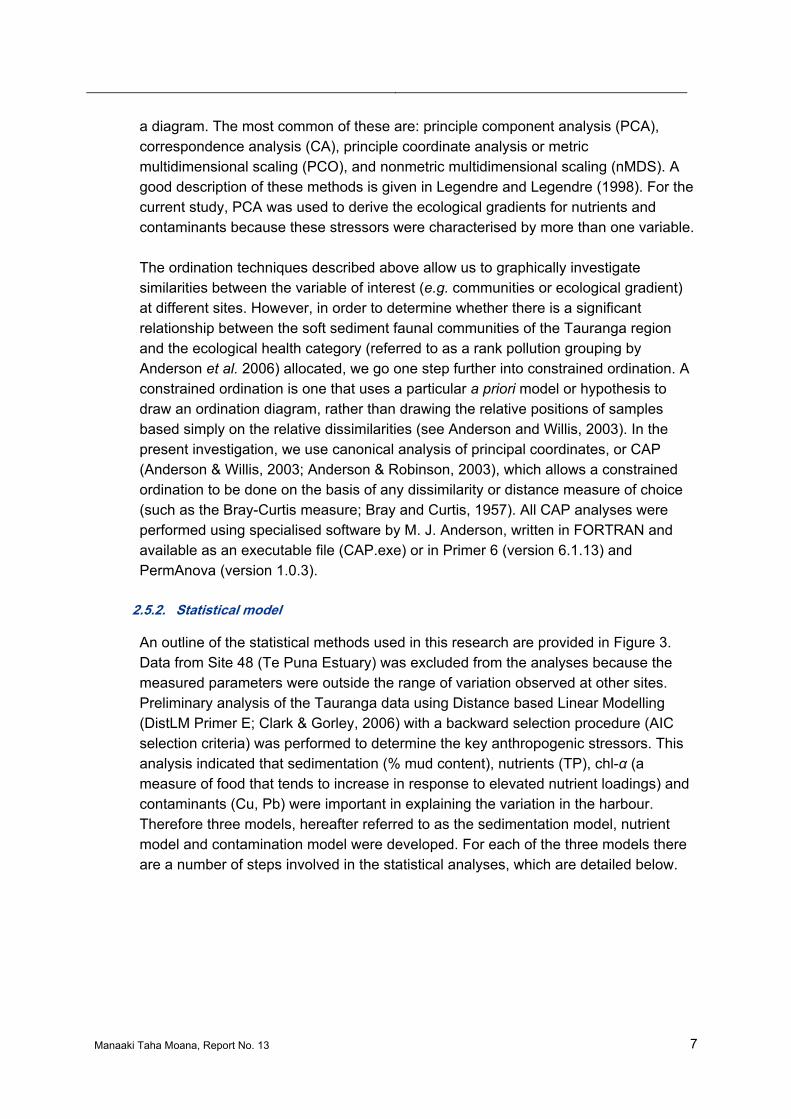
3.3.1. Sedimentation canonical analysis of principal coordinates model

A strong gradient of community change was observed in response to mud content of the sediment (R2 = 0.7683) suggesting that this BHM can be used to determine potential effects of changes in sediment mud content. Most of the sites (41%) were ranked in ecological health category ‘2’, suggesting fairly healthy communities with regard to sedimentation (Figure 13; Figure 14). The environmental health index, based on biotic assemblages, was closely related to the percentage mud content in the sediment, with the muddiest sites (14-49% mud) ranked as ‘5’ and sandiest sites


as ‘1’ or healthy (0.6-9.5% mud; Table 3). The organic content of the sediment also tended to increase with increasing ecological health category, reflecting the tendency of organic material to accumulate in fine sediments. Sites in category ‘5’ (11% of sites), the most impacted ecological health category, were found in inner estuaries (Figure 14) where deposition of sediments would be expected to be highest. Conversely, sites in categories ‘1’ and ‘2’ tended to be in outer areas of the harbour. Interestingly, sites closest to the Wairoa sub-catchment (Sites 54, 55 and 56), the largest sub-catchment and therefore greatest contributor of sediment to the southern harbour (46% of total load; Elliott et al. 2010), did not show particularly high ecological health values for sedimentation (category ‘3-4’). However, sites in estuaries near smaller, but higher sediment yielding, sub-catchments (e.g. Apata, Te Puna, Wainui) did show correspondingly high ecological health values.

Figure 13. Canonical analysis of principal coordinates (CAP) for mud versus percentage silt and clay

in sediment (mud) for 75 sites in Tauranga Harbour (1 mm + 500 µm model). Red dashed lines demarcate the five sedimentation ecological health categories with ‘1’ indicating a ‘healthy’ community and ‘5’ indicating an ‘impacted’ community.


Figure 14. Canonical analysis of principal coordinates (CAP) for sedimentation (1 mm + 500 µm

model) in Tauranga Harbour for 75 sites. Colours indicate the ecological health categories where a green (low) ranking indicates a low effect of sedimentation (‘healthy’) and a red (high) ranking indicates a high effect (‘impacted’). Major rivers and streams entering the Harbour are shown in blue.

Ecological health category

!( 1

!( 2

!( 3

!( 4

!( 5

!(

!(!(!( !(

!(

!(

!(

!(

!(

!(

!(!(

!(

!(

!(

!(

!(

!(

!(

!(

!(!(

!(!(!(!(!(

!(!(

!(

!(!(!(

!(!(!(

!(

!(

!(!( !(

!(

!(

!(!(

!( !(!(

!(

!(

!(

!(

!(!(

!(

!(

!( !(!(

!(!(!(

!(

!(

!(

!(

!(!(

!( !(!(

!(

!(

9

8

7

6

543 2

1

75

74

737271

7069

68

67

6665646362

616059

58

5756

55

54

53

52

51

5049

48

47

46 45

44

43

424140

39

38

37 3635

343332

31

302928 27 26 2524

2322

21

20

19

18

17

16

15

14

13 12

11

10

±NorthIsland

Bowentown

0 2.5 5 7.5 101.25km

Mt Maunganui

Sedimentation 1mm + 500µm infauna

'healthy'

'impacted'


Table 3. Sedimentation ecological health categories (1 mm + 500 µm model) for 75 sites in the Tauranga Harbour and corresponding ranges for key variables for each group. AFDW = ash-free dry weight, chl-α = chlorophyll-α, N = total abundance per core, S = total number of taxa per site, J = Pielou’s evenness, H = Shannon-Wiener index.

Category Sites % gravel % sand %

silt/clay % AFDW Chl-α (µg/kg) N S J H

‘Hea

lth

y’

1 2, 8, 25, 45, 53, 60, 71

< 0.1–14.6 82.8–99.3 0.6–9.5 0.9–3.1 3600–11000 46–267 16–34 0.5–1.0 1.5–2.4

2

1, 3, 4, 5, 6, 9, 15, 16, 17, 18, 19, 20, 21, 30, 32, 33, 34, 35, 43, 52, 59, 61, 63, 64, 65, 66, 67, 73, 74

< 0.1–6.4 62.7–100 < 0.1–100 0.9–3.8 210–11000 29–263 17–39 0.5–0.9 1.6–3.0

3

7, 11, 12, 24, 28, 29, 31, 36, 39, 41, 44, 49, 51, 55, 56, 57, 62, 68, 70, 72, 75

0.1–7.1 77.2–95.7 3.8–22.4 2.0–4.3 1900–16000 57–333 10–39 0.08–0.8 0.2–2.9

‘Imp

acte

d’ 4

14, 22, 23, 26, 27, 42, 50, 54

< 0.1–3.9 51.6–87.6 10.9–34.2 3.1–4.5 3300–9600 61–133 13–33 0.4–0.8 1.1–2.7

5 10, 13, 37, 38, 40, 46, 47, 69

0.2–10.2 50.7–85.1 14.3–48.9 3.1–4.5 2800–8800 35–109 14–25 0.4–0.8 1.1–2.4

Note: Site 48 excluded from CAP analysis because it was an outlier (outside the range of variation observed at the other sites).


Infauna numbers were highest at the healthy category ‘1’ sites (mean 145 per core, range 46-267) and lowest at the impacted category ‘5’ sites (mean 66 per core, range 35-109; Table 3). Species richness was similar in the first four categories (means of 23-28 taxa per site) but slightly lower at category ‘5’ sites (mean 19 taxa per site). The key species differences at healthy versus impacted sites along an increasing gradient of siltation are provided in Table 4. Key species associated with high silt and clay included the polychaete worms Nereididae, Scolecolepides benhami and Heteromastus filiformis and the deposit feeding bivalve Arthritica bifurca. Key benthic species associated with low silt and clay included the worms Scoloplos cylindrifer and Scolelepis sp., the gastropod Halopyrgus pupoides and Oligochaete worms.


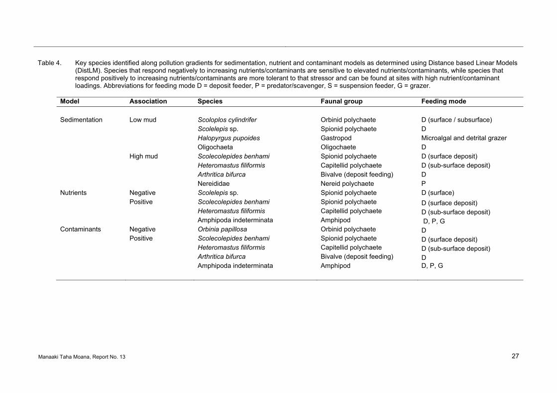
Table 4. Key species identified along pollution gradients for sedimentation, nutrient and contaminant models as determined using Distance based Linear Models (DistLM). Species that respond negatively to increasing nutrients/contaminants are sensitive to elevated nutrients/contaminants, while species that respond positively to increasing nutrients/contaminants are more tolerant to that stressor and can be found at sites with high nutrient/contaminant loadings. Abbreviations for feeding mode D = deposit feeder, P = predator/scavenger, S = suspension feeder, G = grazer.

Model Association Species Faunal group Feeding mode

Sedimentation Low mud Scoloplos cylindrifer Orbinid polychaete D (surface / subsurface) Scolelepis sp. Spionid polychaete D Halopyrgus pupoides Gastropod Microalgal and detrital grazer Oligochaeta Oligochaete D High mud Scolecolepides benhami Spionid polychaete D (surface deposit) Heteromastus filiformis Capitellid polychaete D (sub-surface deposit) Arthritica bifurca Bivalve (deposit feeding) D Nereididae Nereid polychaete P Nutrients Negative Scolelepis sp. Spionid polychaete D (surface) Positive Scolecolepides benhami Spionid polychaete D (surface deposit) Heteromastus filiformis Capitellid polychaete D (sub-surface deposit) Amphipoda indeterminata Amphipod D, P, G Contaminants Negative Orbinia papillosa Orbinid polychaete D Positive Scolecolepides benhami Spionid polychaete D (surface deposit) Heteromastus filiformis Capitellid polychaete D (sub-surface deposit) Arthritica bifurca Bivalve (deposit feeding) D Amphipoda indeterminata Amphipod D, P, G


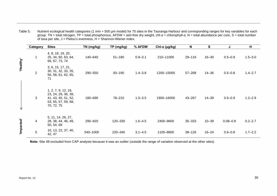
3.3.2. Nutrient canonical analysis of principal coordinates model

The nutrient CAP model was based on a constrained ordination of benthic community taxa in relation to the ecological gradient (PCnut) generated from the concentrations of TN, TP and chl-α at each site. A gradient of community change was observed in response to nitrogen, phosphorous and chl-α concentrations in the sediment suggesting that the BHM can be used to determine potential effects of changes in nutrient concentrations. Most of the sites (32%) were ranked in ecological health category ‘3’ (Figure 15; Figure 16). The level of impact from nutrients was closely related to concentrations of nitrogen and phosphorous in the sediment, with lower nutrient concentrations at category ‘1’ sites (means of 321 and 157 mg/kg for TN and TP) than category ‘5’ sites (means of 724 and 263 mg/kg for TN and TP; Table 5). Organic content also tended to increase along the nutrient gradient. Sites in categories ‘4’ and ‘5’, the most impacted categories, were generally found in estuaries along the inner coast of the harbour, whereas sites ranked lower tended to be situated in the outer harbour (Figure 16). While this CAP model was generated from a significant community response to a nutrient gradient, its correlation was the lowest (R2 = 0.5135) compared to the CAP models for sediments and contaminants.

Figure 15. Canonical analysis of principal coordinates (CAP) for nutrients versus the PC1 axes

derived from sediment nutrient data (TN, TP, chl-α) for 75 sites in Tauranga Harbour (1 mm + 500 µm model). Red dashed lines demarcate the five ecological health categories with ‘1’ indicating a ‘healthy’ community and ‘5’ indicating an ‘impacted’ community.


Figure 16. Canonical analysis of principal coordinates (CAP) for nutrients (1 mm + 500 µm model) in

Tauranga Harbour for 75 sites. Colours indicate the ecological health categories where a green (low) ranking indicates a low effect of nutrients (‘healthy’) and a red (high) ranking indicates a high effect (‘impacted’).


!( 1

!( 2

!( 3

!( 4

!( 5

!(

!(!(!( !(

!(

!(

!(

!(

!(

!(

!(!(

!(

!(

!(

!(

!(

!(

!(

!(

!(!(

!(!(!(!(!(

!(!(

!(

!(!(!(

!(!(!(

!(

!(

!(!( !(

!(

!(

!(!(

!( !(!(

!(

!(

!(

!(

!(!(

!(

!(

!( !(!(

!(!(!(

!(

!(

!(

!(

!(!(

!( !(!(

!(

!(

9

8

7

6

543 2

1

75

74

737271

7069

68

67

666564

6362

616059

58

5756

55

54

53

52

51

5049

48

47

46 45

44

43

424140

39

38

37 3635

343332

31

302928 27 26 2524

2322

21

20

19

18

17

16

15

14

13 12

11

10

±NorthIsland

Bowentown

0 2.5 5 7.5 101.25km

Mt Maunganui

Nutrients1mm + 500µm infauna

'healthy'

'impacted'

Report No. 13 30

Table 5. Nutrient ecological health categories (1 mm + 500 µm model) for 75 sites in the Tauranga Harbour and corresponding ranges for key variables for each group. TN = total nitrogen, TP = total phosphorous, AFDW = ash-free dry weight, chl-α = chlorophyll-α, N = total abundance per core, S = total number of taxa per site, J = Pielou’s evenness, H = Shannon-Wiener index.

Category Sites TN (mg/kg) TP (mg/kg) % AFDW Chl-α (µg/kg) N S J H

‘Hea

lth

y’ 1

4, 8, 18, 19, 20, 25, 34, 60, 63, 64, 66, 67, 73, 74

140–640 51–180 0.9–3.1 210–11000 29–116 16–30 0.5–0.9 1.5–3.0

2

3, 6, 15, 17, 21, 30, 31, 32, 33, 35, 56, 58, 61, 62, 65, 71

290–550 93–190 1.4–3.8 1200–15000 57–268 14–36 0.5–0.8 1.4–2.7

3

1, 2, 7, 9, 12, 16, 23, 24, 29, 36, 39, 41, 43, 45, 51, 52, 53, 55, 57, 59, 68, 70, 72, 75

180–690 78–210 1.0–3.5 1900–16000 43–267 14–39 0.5–0.9 1.2–2.9

‘Imp

acte

d’

4 5, 11, 14, 26, 27, 28, 38, 44, 46, 49, 50, 54, 69

290–920 120–330 1.6–4.5 2400–9600 35–333 10–39 0.08–0.8 0.2–2.7

5 10, 13, 22, 37, 40, 42, 47

540–1000 220–340 3.1–4.5 1100–8800 38–126 16–24 0.6–0.8 1.7–2.2



No clear trend in abundances of organisms was apparent with infauna numbers highest at category ‘2’, ‘3’ and ‘4’ sites (means of 141, 124 and 149 per core, respectively) and lowest at category ‘1’ and ‘5’ sites (means of 74 and 69, respectively; Table 5). Species richness was similar in the first four categories (means of 22-28 taxa per site) but slightly lower at category ‘5’ sites (mean 19 taxa per site). The univariate measures were, therefore, in general not as sensitive at detecting differences across the ecological health categories. The polychaete Scolelepsis sp. was associated with high nutrients while key species sensitive to elevated nutrient loadings included the poychaete worms S. benhami and H. filiformis and amphipods (Table 4).

3.3.3. Contamination canonical analysis of principal coordinates model

The contamination CAP model was based on a constrained ordination of benthic community taxa in relation to the ecological gradient (PCcont axis) generated from the concentration of heavy metals (Pb, Cu and Zn) at each site. A strong gradient of community change was observed in response to heavy metal concentrations in the sediment (R2 = 0.7075) suggesting that the BHM can be used to determine potential effects of changes in metal concentrations. Most of the sites (39%) were ranked in ecological health category ‘3’ (Figure 17; Figure 18). All metal concentrations increased with increasing ecological health category (Table 6). The organic content of the sediment (as % AFDW) also tended to increase with increasing environmental health values, reflecting the tendency of metals to bind with fine sediments. As with the other CAP models, category ‘5’ sites tended to be situated in inner harbour areas and category ‘1’ and ‘2’ sites further out.


Figure 17. Canonical analysis of principal coordinates (CAP) for contamination versus the PC1 axes derived from heavy metal concentrations in sediments (Cu, Pb, Zn) for 75 sites in Tauranga Harbour (1 mm + 500 µm model). Red dashed lines demarcate the five ecological health categories with ‘1’ indicating a ‘healthy’ community and ‘5’ indicating an ‘impacted’ community.

-0.3 -0.2 -0.1 0 0.1 0.2 0.3CAPcont

-2

-1

0

1

2'Healthy' 'Impacted'

R2 = 0.7075


Figure 18. Canonical analysis of principal coordinates (CAP) for contamination (1 mm + 500 µm

model) in Tauranga Harbour for 75 sites. Colours indicate the ecological health categories where a green (low) ranking indicates a low effect of contamination (‘healthy’) and a red (high) ranking indicates a high effect (‘impacted’).


!( 1

!( 2

!( 3

!( 4

!( 5

!(

!(!(!( !(

!(

!(

!(

!(

!(

!(

!(!(

!(

!(

!(

!(

!(

!(

!(

!(

!(!(

!(!(!(!(!(

!(!(

!(

!(!(!(

!(!(!(

!(

!(

!(!( !(

!(

!(

!(!(

!( !(!(

!(

!(

!(

!(

!(!(

!(

!(

!( !(!(

!(!(!(

!(

!(

!(

!(

!(!(

!( !(!(

!(

!(

9

8

7

6

543 2

1

75

74

737271

7069

68

67

6665646362

616059

58

5756

55

54

53

52

51

5049

48

47

46 45

44

43

424140

39

38

37 3635

343332

31

302928 27 26 2524

2322

21

20

19

18

17

16

15

14

13 12

11

10

±NorthIsland

Bowentown

0 2.5 5 7.5 101.25km

Mt Maunganui

Contamination1mm + 500µm infauna

'healthy'

'impacted'


Table 6. Contamination ecological health categories (1 mm + 500 µm model) for 75 sites in the Tauranga Harbour and corresponding ranges for key variables for each group. Pb = lead, Cu = copper, Zn = zinc, N = total abundance per core, S = total number of taxa per site, J = Pielou’s evenness, H = Shannon-Wiener index.

‘Hea

lth

y’ Category Sites Pb (mg/kg) Cu (mg/kg) Zn (mg/kg) % silt/clay N S J H

1 4, 19, 25, 35, 45, 67 < 1.0–1.4 < 1.0 5.1–9.5 1.4–7.0 29–132 17–27 0.6–0.8 1.9–2.6

2 2, 3, 5, 6, 8, 15, 16, 17, 18, 20, 21, 30, 53, 60, 66

< 1.0–2.2 < 1.0 < 5.0–17.0 < 0.1–9.5 42–267 16–36 0.5–0.9 1.5–3.0

3

1, 7, 9, 11, 12, 24, 26, 31, 32, 33, 34, 39, 41, 43, 51, 52, 57, 58, 59, 61, 62, 63, 64, 65, 68, 71, 73, 74, 75

< 1.0–4.3 < 1.0–1.7 7.5–45.0 1.8–23.3 43–263 14–39 0.5–0.8 1.5–2.9

‘Imp

acte

d’

4

13, 22, 23, 27, 28, 29, 36, 37, 38, 40, 42, 44, 46, 47, 49, 54, 56, 70, 72

2.5–5.4 < 1.0–2.2 14.0–55.0 10.3–48.9 35–333 10–39 0.08–0.8 0.9–2.9

5 10, 14, 50, 55, 69 4.2–5.6 1.1–3.0 21.0–44.0 12.6–32.4 96–138 13–31 0.4–0.7 1.1–2.4



Infauna numbers were lowest at category ‘1’ sites (mean 78 per core, range 29-132) and highest at category ‘2’ sites (mean 139 per core, range 42-267; Table 6). Species richness did not differ across the first four categories (means of 23-28 taxa per site) and was reduced only at the most polluted sites (category ‘5’; mean 18 taxa per site). Again the univariate measures in general were not as sensitive as the multivariate ordinations at detecting differences across the ecological gradient. Key species associated with high contaminant loadings included the polychaete worm Orbinia papillosa while species sensitive to elevated contaminant loadings included the polychaete worms S. benhami, H. filiformis, amphipods and the deposit feeding bivalve A. bifurca (Table 4).


3.4. Species response curves

Most species displayed clear differences in abundance as a function of sediment type, nutrient loading or contaminant levels. The models revealed a wide variety of functional forms, indicating that the occurrence of species is influenced by species-specific sensitivity to mud content, nutrients or contaminants. Sandy sediments were dominated by bivalve species, including the cockle (A. stutchburyi), the wedge shell (Macomona liliana) and the nut shell (Nucula hartvigiana), and also by the polychaete worms O. papillosa and S. cylindrifer (Figure 20). Some species, including the small bivalve A. bifurca and predatory Nereididae worms, exhibited polynomial response models, reflecting the highest probability of occurrence at intermediate mud content (Figure 19; Figure 20). However, beyond a certain level of increasing mud content their abundances decreased. For increasing nutrient levels many species exhibited polynomial response curves, with an increase in abundance associated with nutrient loading followed by a decrease in abundance levels beyond critical levels. Species exhibiting polynomial response curves included the bivalves A. bifurca, A. stutchburyi, N. hartvigiana and M. liliana as well as the polychaete worms S. benhami, H. filiformis and Nereididae (Figure 21; Figure 22). Increasing sediment contamination levels from heavy metals resulted in decreasing abundance for the bivalves A. bifurca, A. stutchburyi, M. liliana and the polychaetes O. papillosa, S. cylindrifer and Scolelepsis sp. (Figure 23; Figure 24).

Figure 19. Relationship between taxa abundance and log percentage mud in ambient sediment.

No.

per

cor

e

ln (%mud)

Nereididae


Figure 20. Relationship between taxa abundance and percentage mud in ambient sediment. P

values indicate significance of trend, with no trend line displayed if the trend was not significant (p > 0.1).

5 10 15 20

0.0

0.1

0.2

0.3

0.4

0.5

dens

ity, n

umbe

r pe

r co

reArthritica bifurca

p > 0.1

5 10 15 20

010

2030

4050

Austrovenus stutchburyi

p < 0.001

5 10 15 20

1020

30

Heteromastus filiformis

p < 0.001

5 10 15 20

02

46

8

dens

ity, n

umbe

r pe

r co

re

Macomona liliana

p = 0.0056

5 10 15 20

010

2030

40Nucula hartvigiana

p < 0.001

5 10 15 20

0.00

0.05

0.10

0.15

0.20

Oligochaeta

p > 0.1

5 10 15 20

01

23

45

dens

ity, n

umbe

r pe

r co

re

Orbinia papillosa

p < 0.001

5 10 15 20

24

68

1014

% mud

Scolecolepides benhami

p > 0.1

5 10 15 20

0.0

0.2

0.4

0.6

0.8

% mud

Scolelepis sp.

p > 0.1

5 10 15 20

01

23

45

67

% mud

dens

ity, n

umbe

r pe

r co

re

Scoloplos cylindrifer

p < 0.001


Figure 21. Relationship between taxa abundance and log nutrient concentrations in ambient

sediment.

ln (PCnut) ln (PCnut)

ln (PCnut) ln (PCnut)

No.

per

cor

e

No.

per

cor

e

Arthritica bifurca Austrovenus stutchburyi

Nucula hartvigiana Scolecolepides benhami


Figure 22. Relationship between taxa abundance and nutrient (PCnut) concentrations in ambient

sediment. P values indicate significance of trend, with no trend line displayed if the trend was not significant (p > 0.1).

5 10 15 20

010

2030

dens

ity, n

umbe

r pe

r co

reHeteromastus filiformis

p > 0.1

5 10 15 20

02

46

8

Macomona liliana

p > 0.1

5 10 15 20

0.00

0.05

0.10

0.15

0.20

Oligochaeta

p > 0.1

5 10 15 20

02

46

dens

ity, n

umbe

r pe

r co

re

Orbinia papillosa

p < 0.001

5 10 15 20

05

1015

nutrient concentration

Nereididae

p = 0.037

5 10 15 20

0.0

0.2

0.4

0.6

0.8


Scolelepis sp.

p > 0.1

5 10 15 20

02

46


dens

ity, n

umbe

r pe

r co

re


p = 0.001


Figure 23. Relationship between taxa abundance and log contaminant levels in ambient sediment.

ln (PCcont) ln (PCcont)

No.

per

cor

e

No.

per

cor

e

Nucula hartvigiana

Scolecolepides benhami


Figure 24. Relationship between taxa abundance and log contaminant (PCcont) concentrations in

ambient sediment. P values indicate significance of trend, with no trend line displayed if the trend was not significant (p > 0.1).

0 5 10 15 20 25 30

0.0

0.2

0.4

0.6

dens

ity, n

umbe

r pe

r co

reArthritica bifurca

p > 0.1

0 5 10 15 20 25 30

010

2030

4050

Austrovenus stutchburyi

p < 0.001

0 5 10 15 20 25 30

010

2030

Heteromastus filiformis

p < 0.001

0 5 10 15 20 25 30

02

46

8

dens

ity, n

umbe

r pe

r co

re

Macomona liliana

p = 0.0112

0 5 10 15 20 25 30

0.00

0.05

0.10

0.15

0.20

Oligochaeta

p > 0.1

0 5 10 15 20 25 30

02

46

Orbinia papillosa

p < 0.001

0 5 10 15 20 25 30

05

1015

contaminant concentration

dens

ity, n

umbe

r pe

r co

re

Nereididae

p = 0.0327

0 5 10 15 20 25 30

0.0

0.2

0.4

0.6

0.8


Scolelepis sp.

p > 0.1

0 5 10 15 20 25 30

02

46



p < 0.001


4. DISCUSSION

In this report we summarise the results from a broad scale survey of the Tauranga Harbour that assessed both the health of macrofaunal benthic communities (bottom-dwelling animals) as well as trends in sediments, nutrients and contaminants. Sites identified as most impacted were generally located in the upper reaches of estuaries in some of the locations least exposed to wind, waves and currents. To some extent, this reflects the natural progression of an estuary from land to sea (for example, higher sedimentation close to the coast), however, the rates of accumulation of sediments and nutrients have been accelerated as a result of anthropogenic land-based activities. In addition, the community composition and key species characterizing sites with different sediment textures, nutrient and contaminant loadings were found to vary. Using community data we developed ordination models of ecological health for sediments, nutrients and contaminants. Before discussing the results of these community-based models we first summarize general trends in sedimentation, nutrients and contaminants that were recorded within Tauranga Harbour.

4.1. Physical patterns of elevated sediments, nutrients and heavy metal contamination

Sediments within Tauranga Harbour were found to be predominantly sandy with the percentage of mud within a similar range as measured for other New Zealand estuaries (Table 7). The exceptions included Te Puna and Apata Estuaries, which showed higher rates of sedimentation consistent with previous studies. The inner Te Puna Estuary was identified by Hume et al. (2010) as the most depositional sub-estuary in the southern harbour with net accumulation of 6.51 mm y-1. Similarly, Park (2003) and Hancock et al. (2009) identified the Apata Estuary as one of the muddiest areas of the harbour. Modeling of sediment loads into the southern Tauranga Harbour identified both the Te Puna and Apata sub-catchments as having relatively high sediment yields, with the Apata sub-catchment yielding the most sediment of all the sub-catchments modeled due to the relatively high rainfall in conjunction with pasture land use and moderate slopes (Elliott et al. 2010).


Table 7. Comparison of average particle size and nutrient characteristics of sediments sampled during the present survey with previously reported values for some other New Zealand estuaries. Mean values are displayed with estuary ranges in brackets beneath. Mud-dominated sites are shaded.

Location Sand Mud AFDW TN TP TN:TP General estuary

condition/health % % % mg/kg mg/kg Molar Tauranga Harbour (present study) Sand-dominated sites 85

(51-100) 13

(1–49) 2.8

(0.9–4.5) 462

(140–1000) 164

(51–340) 6.4

slightly to moderately enriched

Mud–dominated site (enriched) a 24 76 10 1900 580 7.3 enriched Other NZ estuaries

Kaipara (Otamatea Arm site C) b 50 (38–56)

33 (21–55)

4.5 (3.1–6.5)

1192 (800–1800)

572 (547–605)

4.6 moderately enriched

Ohiwa c 77 (53–92)

20 (7–44)

2.0 (0.7–3.7)

650 (250–1000)

278 (212–350)

5.1 slight to moderately enriched

Ruataniwha d 86

(67–94) 9

(6–18) 1.2

(0.5–1.7) 263

(250–700) 458

(330–580) 1.3

slightly enriched

Waimea c 74 (25–93)

24 (7–70)

1.4 (0.3–2.8)

506 (250–1000)

433 (243–562)

2.6

slight to moderately enriched

Havelock e 77 (68–85)

19 (13–26)

1.6 (0.7–2.3)

422 (70–900)

330 (241–433)

2.8


Avon–Heathcote d 94

(90–97) 5

(3–9)

1.0 (0.5–1.3)

301 (250–600)

327 (298–355)

2.0

moderately enriched

Kaikorai f 70

(61–78) 27

(20–33) 5.1

(3.9–6.9) 1650

(1500–2100) 799

(728–913) 4.6

moderately enriched but contaminant affected

New River c 98

(96–99) 2

(1–3) 0.6

(0.3–1.4) 250

(250–250) 280

(195–432) 2.0

non-enriched

Delaware (sites B, C) g

88 (79–98)

11 (2–20)

2.2 (1.9–2.3)

282 (230–310)

558 (540–580)

0.5

relatively undisturbed, naturally productive

Nelson Haven h 87

(78–93) 12

(7–18) 1.4

(1.0–1.8) 276

(140–440) 339

(240–460) 1.8

very slightly enriched


Location Sand Mud AFDW TN TP TN:TP General estuary condition/health

% % % mg/kg mg/kg Molar Moutere i 88

(83–91) 12

(8–15) 1.6

(0.6–2.0) 339

(280–450) 530

(474–590) 1.4


Moutpipi j 70

(54–86) 30

(13–47) 2.3

(1.8–2.8) 743

(570–990) 565

(520–600) 2.9

moderately enriched

Kaipara (Otamatea Arm sites A, B) k 27 (15–39)

68 (52–73)

6.3 (1.7–7.8)

1850 (1600–2400)

503 (443–619)

8.1

moderately enriched

Delaware (site A) l 26

(24–29) 73

(71–76)

3.4 (2.6–4.3)

823 (790–850)

587 (530–630)

3.1

relatively undisturbed, naturally productive

Orowaiti m 42

(32–47) 53

(42–60) 3.2

(1.6–5.1) 794

(590–1200) 938

(770–1040) 1.9

slightly to moderately enriched

Waimea n 82.5 9.1 4340 1063 8.9 highly enriched (highly enriched site—historical data)

a Highly enriched site (Te Puna)

b Subset of sand-dominated sites from an inter-estuary comparison, 2001 (Robertson et al. 2002b).

c Mean of four sand-dominated sites from an inter-estuary comparison, 2001 (Robertson et al. 2002b).

d Mean of three sand-dominated sites from an inter-estuary comparison, 2001 (Robertson et al. 2002b).

e Mean of two sand-dominated sites from an inter-estuary comparison, 2001 (Robertson et al. 2002b).

f Mean of one sand-dominated site from an inter-estuary comparison, 2001 (Robertson et al. 2002b).

g Subset of sand-dominated sites, 2009 (Gillespie et al. 2009).

h Mean of three sand-dominated sites, 2012, (Gillespie et al. 2012).

i Mean of two sand-dominated sites, 2006 (Gillespie & Clark, 2006).

j Mean of two sand-dominated sites, 2008 (Robertson & Stevens, 2008).

k Subset of mud-dominated sites from an inter-estuary comparison, 2001 (Robertson et al. 2002b).

l Subset of mud-dominated sites, 2009 (Gillespie et al. 2009).

m Mean of two mud-dominated estuaries, 2007 (Gillespie & Clark, 2007).

n Mudflat affected by a freezing works effluent, 1981 (Gillespie & MacKenzie 1990).


Nutrient and organic matter concentrations in the harbour tended to decline with distance from the inner harbour region and associated rivers. Sediment nitrogen, phosphorus and organic content are indicators of organic nutrient enrichment that are often closely linked with sediment grain size. In general terms, higher nutrient and organic concentrations are usually associated with muddier substrata. This relationship may partially explain the comparatively high organic content and nutrient loadings at Te Puna Estuary (Table 7). Comparison of sediment nutrient concentrations with other New Zealand estuaries (Table 7) indicates that the Tauranga Harbour sits within a range typical for slightly to moderately enriched estuarine conditions. Although sediment phosphorous concentrations were low in Tauranga Harbour compared with other estuaries, the total N:P ratios indicated that the estuary was still limited by nitrogen. Recent studies have found that levels of nitrogen and phosphorus have changed little within Tauranga Harbour between the early 1990s and 2005 (see Sinner et al. 2011). Most major point source discharges of nitrogen and phosphorous (such as sewage outfalls) were removed from the harbour in the early to mid-1990s. Nutrient levels in many of the rivers and streams entering the harbour have declined due to improved rural practices and better control of surface runoff and land use changes. However, many of these rivers still have elevated nutrient levels, and some show increasing trends associated with agriculture and runoff from recently harvested forest (Scholes, 2005; Sinner et al. 2011). The low residence times within Tauranga Harbour (see Heath, 1976) result in rapid dilution of nutrients. The flushing rates largely mitigate seabed enrichment effects in the central and outer regions of the harbour, with localised seabed enrichment effects occurring near source streams.

Sediment contamination by heavy metals can also be highly correlated with the percentage of mud content due to the adherence of chemicals to fine sediments and/or organic content (see Green et al. 2001). It is, therefore, not surprising that heavy metal concentrations were highest in the depositional inner areas of the harbour, such as Te Puna Estuary. Acceptably low levels of copper, lead and zinc were found throughout Tauranga Harbour compared with ANZECC (2000a) ISGQ trigger guidelines and the TELs (threshold effects level 18.7, 30.2 and 124 for copper, lead and zinc respectively) developed by MacDonald et al. (1996) and utilised by the Auckland Council. Although the three metals recorded were found to be highly correlated, zinc levels tended to be closer to guideline thresholds indicating possible biological effects. This trend was also reported for the Auckland region (Anderson et al. 2002). Comparison with other New Zealand and overseas estuaries showed Tauranga Harbour is performing well with respect to heavy metal contamination (Table 8).


Table 8. Concentrations of trace metals in sediments from Tauranga Harbour and a selection of New Zealand and overseas estuaries that have been contaminated to varying degrees. Some values drawn from other studies are approximate as they were estimated from figures.

Location Cu Pb Zn

mg/kg mg/kg mg/kg ANZECC (2000a) ISQG-Low 65 50 200 ANZECC (2000a) ISQG-High 270 220 410

Tauranga (present study)

All sites except 48 1.5 (< 1–3) 2.6 (< 1–5.6) 17.2 (< 5–55)

Site 48 6.1 13.0 46.0

EMP development Kaipara (Otamatea Arm) 13.8 11.4 54.5

study a Ohiwa 4.0 3.4 27.7

Ruataniwha 7.1 4.7 37.5

Waimea 9.6 7.4 41.8

Havelock 10.7 5.6 43.0

Avon–Heathcote 3.2 6.3 38.3

Kaikorai 16.8 45.3 184.2

New River 3.8 0.7 17.1

Other NZ Delaware Inlet b 11.0 3.8 45.3

sites Moutere Inlet c 6.1 4.2 25.9

Nelson Haven d 5.5 3.8 24.3

Motupipi Estuary e 7.7 5.1 35.7

Orowaiti Estuary f 1.8 4.3 44.6

Tamaki A (E1) g 27.8 132.1 136.1

Tamaki B (E2) g 26.1 72.9 167

Tamaki C (E3) g 29.4 69.7 173

Tamaki D (E4) g 38.5 145.2 233

Manukau (rural catch) h 20 9 114

Manukau (industrial catch) h 90 58 285

Waitemata Harbour i 60 65 161

Lambton Harbour, Wellington j 68 183 249

Porirua Harbour, Wellington k 48 93 259

Aparima Estuary l 12 11 49

Mataura Estuary l 6.6 6.2 27 Overseas sites Delaware Bay, USA m 8.3 15 49.7

Lower Chesapeake Bay, USA m 11.3 15.7 66.2

San Diego Harbour, USA m 218.7 51 327.7

Salem Harbour, USA m 95.1 186.3 238

Rio Tinto Estuary, Spain l 1400 1600 3100

Restronguet Estuary, UK l 4500 1620 3000

Nervión Estuary, Spain n 50–350 50–400 200–2000

Sorfjord, Norway m 12000 30500 118000

Sources: a (Robertson et al. 2002b), b (Gillespie et al. 2009), c (Gillespie and Clark, 2006), d (Gillespie et al. 2012), e (Robertson and Stevens, 2008), f (Gillespie and Clark, 2007), g (Thompson, 1987), h (Roper et al. 1988), i (Glasby et al. 1988), j (Stoffers et al. 1986), k (Glasby et al. 1990), l (Robertson, 1995), m (Kennish, 1997), n (Jezus-Belzunce et al. 2001).


4.2. Community based models

We used ordination modelling approaches to identify key stressors affecting the ‘health’ of macrofaunal communities In Tauranga Harbour. Sediments, nutrients and heavy metals were identified as key ‘stressors’, i.e. variables affecting the ecology of the harbour. Therefore, three models were developed based on the variability in community composition using CAP analyses. The ecological assemblages generally reflected gradients of stress or pollution very well. However, the CAP models for sediments and contaminants performed better than for nutrients. The multivariate models were found to be more sensitive to changing environmental health than simple univariate measures (abundance, species diversity, Pielou’s evenness and Shannon-Wiener diversity). For sedimentation, univariate measures did detect changes in abundance and species richness between the most and least disturbed sites. However, for the nutrient and contaminant models the univariate measures only observed differences in species richness at the least healthy sites. No clear patterns in the other univariate measures along the ecological gradient were observed. This trend has also been reported in the literature where univariate measures found significant differences between the most and least disturbed sites, but none of them were able to differentiate between smaller relative differences (Attayde and Bozelli, 1998). It has, therefore, been recommended that utilizing all of the information on the abundance of each taxon can increase the sensitivity and allow a more ecologically meaningful response to be observed (Attayde & Bozelli, 1998, this study; Gray, 2000; Hewitt et al. 2005; Pohle et al. 2001). For Tauranga Harbour, constrained ordination models based on community composition appear to be a more sensitive measure than univariate measures of ‘health’ along an ecological gradient and should enable long term degradative change from multiple disturbances to be assessed. For all three analyses, a significant model relating changes in communities to changes in the environmental measures were able to be developed. This approach can be used as a management or monitoring tool where sites are repeatedly sampled over time and tracked to determine whether the communities are moving towards a more healthy or unhealthy state. New observations can also be placed into the model and community ‘health’ can be defined based on its position in the ordination space. Hence new sites can be placed into the canonical space in future (Anderson & Robinson, 2003) and sites can be monitored over time to assess long term degradation or improvement in the ecology of an area. Multivariate analysis based on all taxa also gives the ability to investigate which taxa are associated with changing environmental health (Hewitt et al. 2005). The key species at ‘healthy’ and ‘impacted’ sites as determined from the CAP models were identified. Species at ‘impacted’ sites can be considered to be tolerant to the stressor


(i.e. sediment, nutrients or contaminants), while species with high abundances at ‘healthy’ sites only are sensitive to increasing stressors. We also modelled the upper quantiles of abundances of populations in an effort to investigate limiting factors acting as constraints on organisms (Landcaster & Belyea, 2006). Models were developed for key species identified in the ordination models and culturally important shellfish species. In ecology, a common phenomenon is for data points to be scattered beneath an upper (or above a lower) limit described as a ‘factor ceiling’ (Thomson et al. 1996). The ceiling to the data scatter implies a constraining factor, thus the form the ceiling takes allows us to derive maximum (or minimum) possible response curves to an environmental variable. This implies that over broad scales, while a number of factors (e.g. the potential for recruitment, historical conditions etc.) may affect the observed density, there is a limit (frequently an upper limit) that is controlled by the variable of interest. Our research results suggest that factor ceiling responses occurred at critical levels of sedimentation, nutrients and contaminants for key shellfish species modelled within Tauranga Harbour. Shellfish response curves were either negative or polynomial. A negative relationship means that as the stressor increases the abundance of a species decreases. For example, as silt/clay content increased the abundance of cockle (A. stutchburyi), wedge shell (M. liliana) and nut shell (N. hartvigiana) populations all decreased. A polynomial response curve results in an increase in abundance associated with elevated stressor levels followed by a decrease in abundance beyond critical stressor levels. For example, the shellfish A. bifurca exhibited such a polynomial response surface, increasing in abundance with increasing percent mud content followed by a decrease in abundance as sediment loading continued to increase. Therefore, most shellfish species populations are either sensitive to elevated silt/clay, nutrient loading or contaminants, or sensitive to these stressors beyond a critical point. The other key species modelled included polychaete worms and their response curves to various stressors varied by species. Elevated sediment loading to estuaries and coastal environments can lead to broad scale changes in ecology through modifying habitats (e.g. Saiz-Salinas & Urkiaga-Alberdi, 1999; Smith & Kukert, 1996) and, in particular, by influencing the health, abundance and distribution of benthic suspension feeders (Ellis et al. 2002). Increased concentrations of silts and clay in suspension may significantly increase pseudofaeces production, decrease the amount of algal food actually ingested, and may also damage bivalve gills (Bricelj & Malouf, 1984; Iglesias et al. 1996; Morse et al. 1982; Navarro et al. 1992; Navarro & Widdows, 1997; Robinson et al. 1984; Stevens, 1987; Willows, 1992). Exposure to increased concentrations of suspended sediments for an extended time can, therefore, result in decreased amounts of energy available for growth and reproduction, and have deleterious effects on local populations.


Low levels of nutrient enrichment in estuarine and coastal environments can have a positive effect on the benthos due to improved primary productivity, and therefore food availability. However beyond a critical point, excessive nutrient discharges can lead to accelerated eutrophication of coastal environments and adverse symptoms of over enrichment (Cloern, 2001; McGlathery et al. 2007). Metals can be essential for organisms as trace elements, however, at higher concentrations they can become toxic (ANZECC, 2000b). High exposure to heavy metals can cause physiological stress, reduced reproductive success, and outright mortality in associated invertebrates and fishes (Fleeger et al. 2003; Gagnaire et al. 2004; Nicholson, 1999; Peters et al. 1997; Radford et al. 2000). The results from this study were consistent with Thrush et al. (2003) who developed models of macrofaunal species occurrence with respect to sediment mud content. Thrush et al. (2003) found similar responses whereby sensitive species with a preference for low mud content included the mobile suspension feeding cockle and the deposit and suspension feeding nut shell. Within this report we extend this analysis by also developing models of macrofaunal species occurrence with respect to nutrient and contaminants loadings as well as sediment mud content. Ultimately such statistical models provide a tool to forecast the distribution and abundance of species associated with habitat changes in sediments, nutrients and metals.

4.3. Conclusion

Tauranga Harbour is a predominantly sandy harbour with slight to moderate enrichment and low levels of heavy metal contaminants. The community composition and key species characterizing sites with different sediment textures, nutrient and contaminant loadings were found to vary. Te Puna Estuary (Site 48) was found to have high levels of mud, nutrients and heavy metals, outside the range of variation observed at other sites. Sediments, nutrients and heavy metals were identified as key ‘stressors’ or variables affecting the ecology of the harbour. Sediments and contaminants were found to explain the largest variance in benthic communities. Sites classified as most impacted were generally located in the upper reaches of estuaries in some of the least exposed locations. In general, the multivariate models were found to be more sensitive to changing environmental health than simple univariate measures. Species response curves suggest that shellfish are negatively affected by increasing sediments, nutrients and metals beyond critical levels while polychaete responses are species specific. This BHM approach, initially developed by Auckland Regional Council (in conjunction with University of Auckland and NIWA), can be used as a management or monitoring tool where sites are repeatedly sampled over time and tracked to assess long term degradation or improvement in the ecology of an area.


5. REFERENCES

Anderson M, Hewitt J, Thrush S 2002. The Development of Criteria for Assessing Community Health of Urban Intertidal Flats, NIWA report prepared for Auckland Regional Council Technical Report No. 184. pp. 54 plus appendices.

Anderson M.J. 2008. Animal-sediment relationships re-visited: Characterising species' distributions along an environmental gradient using canonical analysis and quantile regression splines. Journal of Experimental Marine Biology and Ecology 366:16-27.

Anderson MJ, Gribble NA 1998. Partitioning the variation among spatial, temporal and environmental components in a multivariate dataset. Australian Journal of Ecology 23:158-167.

Anderson MJ, Willis TJ 2003. Canonical analysis of principal coordinates: a useful method of constrained ordination for ecology. Ecology 84:511-525.

Anderson MJ, Robinson J 2003. Generalized discriminant analysis based on distances. Australian and New Zealand Journal of Statistics 45:301-318.

Anderson MJ, Hewitt JE, Ford RB, Thrush SF 2006. Regional models of benthic ecosystem health: predicting gradients from biological data, Prepared by Auckland UniServices Limited for Auckland Regional Council. Auckland Regional Council Technical Publication 317.

ANZECC 2000a. Australian and New Zealand Guideliens for Fresh and Marine Water Quality - Volume One: the guidelines, Australian and New Zealand Environment and Conservation Council and Agriculture and Resource Management Council of Australia and New Zealand.

ANZECC 2000b. Australian and New Zealand Guidelines for Fresh and Marine Water Quality - Volume 2: aquatic ecosystems - rationale and background information, Australian and New Zealand Environment and Conservation Council and Agriculture and Resource Management Council of Australia and New Zealand.

Attayde JL, Bozelli RL 1998. Assessing the indicator properties of zooplankton assembages to disturbance gradients by canonical correspondence analysis. Canadian Journal of Fisheries and Aquatic Sciences 55:1789-1797.

Barnett AG 1985. Overview and hydrodynamics. Tauranga Harbour Study: Part I & III, A report for the Bay of Plenty Harbour Board.

Blackburn TM, Lawton JH, Perry JN 1992. A Method of Estimating the Slope of Upper Bounds of Plots of Body Size and Abundance in Natural Animal Assemblages. Oikos 65:107-112.

Borcard DP, Legendre P, Drapeau P 1992. Partialling out the spatial component of ecological variation. Ecology 73:1045-1055.


Bray JR, Curtis JT 1957. An ordination of the upland forest communities of Southern Wisconsin. Ecological Monographs 27:325-349.

Bricelj VM, Malouf RE 1984. Influence of algal and suspended sediment concentrations on the feeding physiology of the hard clam Mercenaria mercenaria. Marine Biology 84:155-165.

Clark KR, Gorley RN 2006. PRIMER v6: User manual/Tutorial, PRIMER-E Ltd, Plymouth, UK.

Clarke KR 1993. Non-parametric multivariate analyses of changes in community structure. Australian Journal of Ecology 18:117-143.

Cloern JE 2001. Our evolving conceptual model of the coastal eutrophication problem. Marine Ecology Progress Series 210:223-253.

Cole RG, Hull PJ, Healy TR 2000. Assemblage structure, spatial patterns, recruitment, and post-settlement mortality of subtidal bivalve molluscs in a large harbour in north-eastern New Zealand. New Zealand Journal of Marine and Freshwater Research 34:317-329.

de Lange WP 1988. Wave climate and sediment transport within Tauranga Harbour, in the vicinity of Pilot Bay, PhD thesis (Earth Sciences) University of Waikato, Hamilton.

Dufrene M, Legendre P 1997. Species assemblages and indicator species: the need for a flexible asymmetrical approach. Ecological Monographs 67:345-366.

Dunn C 1994. Gaps in GAP. Plant Science Bulletin 40:120-121.

Elliott S, Parshotam A, Wadhwa S 2010. Tauranga Harbour sediment study: catchment model results, Prepared for Environment Bay of Plenty by NIWA. Client Report: HAM2009-046, Hamilton.

Ellis J, Cummings V, Hewitt J, Thrush S, Norkko A 2002. Determining effects of suspended sediment on condition of a suspension feeding bivalve (Atrina zelandica): results of a survey, a laboratory experiment and a field transplant experiment. Journal of Experimental Marine Biology and Ecology 267:147-174. DOI: 10.1016/s0022-0981(01)00355-0.

Ellis JI, Schneider DC, Thrush SF 2000. Detecting anthropogenic disturbance in an environment with multiple gradients of physical disturbance, Manukau Harbour, New Zealand. Hydrobiologia 440:379-391.

Fleeger JW, Carman KR, Nisbet RM 2003. Indirect effects of contaminants in aquatic ecosystems. The Science of the Total Environment 317:207-233.

Gagnaire B, Thomas-Guyon H, Renault T 2004. In vitro effects of cadmium and mercury on Pacific oyster, Crassostrea gigas (Thunberg), haemocytes. Fish & Shellfish Immunology 16:501-512.


Gappa JJL, Tablado A, Magaldi NH 1990. Influence of sewage pollution on a rocky intertidal community dominated by the mytilid Brachidontes rodriguezi. Marine Ecology Progress Series 63:163-175.

Gillespie P, Clark K 2006. Moutere Inlet Fine-Scale Benthic Baseline 2006, Prepared for Tasman District Council. Cawthron Report No. 1183. pp. 18.

Gillespie P, Clark K 2007. Orowaiti Estuary Fine-Scale Benthic Baseline 2007, Prepared for West Coast Regional Council. Cawthron Report No. 1274. pp. 19 plus appendices.

Gillespie P, Clement D, Asher R 2009. Delaware Inlet Fine-Scale Benthic Baseline 2009, Prepared for Nelson City Council. Cawthron Report No. 1594. pp. 28.

Gillespie P, Clement D, Clark DE, Asher R 2012. Nelson Haven Fine-Scale Benthic Baseline 2012, Prepared for Nelson City Council. Cawthron Report No. 2209. pp. 22 plus appendices.

Glasby G.P, Moss RL, Stoffers P 1990. Heavy metal pollution in Porirua Harbour, New Zealand. New Zealand Journal of Marine and Freshwater Research 24:233-237.

Glasby GP, Stoffers P, Walters P, Davis KR, Renner RM 1988. Heavy-metal pollution in Manukau and Waitemata Harbours, New Zealand. New Zealand Journal of Marine and Freshwater Research 22:595-611.

Gray JS 2000. The measurement of marine species diversity, with an application to the benthic fauna of the Norwegian continental shelf. Journal of Experimental Marine Biology and Ecology 250:23-49.

Green M, Williamson B, Bull D, Oldman J, MacDonald I, Mills G 2001. Prediction of Contaminant Accumulation in Auckland Estuaries, Auckland Regional Council, Hamilton. pp. 78.

Hancock N, Hume T, Swales A 2009. Tauranga Harbour sediment study: harbour bed sediments, Prepared for Environment Bay of Plenty by NIWA. Client Report: HAM2008-123 Hamilton.

Heath RA 1976. Broad classification of New Zealand inlets with emphasis on residence times. New Zealand Journal of Marine and Freshwater Research:429-44.

Hewitt J, Ellis J 2010. Assessment of the benthic health model, Prepared by Organisation for Auckland Regional Council. Auckland Regional Council TR2010/034.

Hewitt J, Anderson MJ, Thrush SF 2005. Assessing and monitoring ecological community health in marine systems. Ecological Applications 15:942-953.

Hume TM, Green MO, Elliott S 2010. Tauranga Harbour sediment study: assessment of predictions for management, Prepared for Environment Bay of Plenty by NIWA. Client Report: HAM2009-139, Hamilton.


Iglesias JIP, Urrutia MB, Navarro E, Alvarez-Jorna P, Larretxea X, Bougrier S, Heral M 1996. Variability of feeding processes in the cockle Cerastoderma edule (L.) in response to changes in seston concentration and composition. Journal of Experimental Marine Biology and Ecology 197:121-143.

Inglis G, Gust N, Fitridge I, Floerl O, Woods C, Kospartov M, Hayden B, Fenwick G 2008. Port of Tauranga: second baseline survey for non-indigenous marine species (Research Project ZBS2000/04), Prepared for Biosecurity New Zealand by NIWA. Biosecurity Technical Paper No: 2008/0, Wellington.

Jezus-Belzunce M, Solaun O, Franco J, Valencia V, Borja A 2001. Accumulation of organic matter, heavy metals and organic compounds in surface sediments along the Nervion Estuary (northern Spain). Marine Pollution Bulletin 42:1407-1411.

Kennish MJ 1997. Pollution impacts on marine biotic communities, CRC Press, New York. pp. 310.

Landcaster J, Belyea LR 2006. Defining limits to local density: alternative views of abundance-environment relationships. Freshwater Biology 50:2034-2052.

Leathwick JR, West D, Gerbeauz P, Kelly D, Robertson H, Brown D, Chadderton WL, Ausseil A-G 2010. Freshwater Ecosystems of New Zealand (FENZ) Geodatabase: Version One - August 2010 User Guide, Department of Conservation.

Legendre P, Legendre L 1998. Numerical ecology. Second English edition Elsevier, Amsterdam, The Netherlands.

Lengendre P, Legendre L 1998. Numerical ecology. Second English edition Elsevier, Amsterdam, The Netherlands.

MacDonald DD, Carr RS, Calder FD, Long ER, Ingersoll CG 1996. Development and evaluation of sediment quality guidelines for Florida coastal waters. Ecotoxicology 5:253-278.

McGlathery KJ, Sundback K, Anderson IC 2007. Eutrophication in shallow coastal bays and lagoons: the role of plants in the coastal filter. Marine Ecology Progress Series 348:1-18.

Morse PM, Robinson WE, Wehling WE 1982. Effects of sublethal concentrations of the drilling mud components attapulgite and Q-broxin on the structure and function of the fill of the scallop Placopecten magellanicus (Glemlin), in: W. B. Vernberg, et al. Eds.), Physiological Mechanisms of Marine Pollution Toxicity, Academic Press. pp. 235-259.

Navarro E, Iglesias JIP, Ortega MM 1992. Natural sediment as a food source for the cockle Cerastoderma edule (L.): effect of variable particle concentration on the feeding, digestion and the scope for growth. Journal of Experimental Marine Biology and Ecology 156:69-87.


Navarro JM, Widdows J 1997. Feeding physiology of Cerastoderma edule in response to a wide range of seston concentrations. Marine Ecology Progress Series 152:175-186. DOI: 10.3354/meps152175.

Nicholson S 1999. Cytological and physiological biomarker responses from green mussels, Perna viridis (L.) transplanted to contaminated sites in Hong Kong coastal waters. Marine Pollution Bulletin 39:261-268.

Olsgard F, Gray JS 1995. A comprehensive analysis of the effects of offshore oil and gas exploration and production on the benthic communities of the Norwegian continental shelf. Marine Ecology Progress Series 122:277-306.

Park SG 2003. Marine sediment and contaminants survey (2001-03) of Tauranga Harbour, Environment Bay of Plenty Environmental Publication 2003/20, Whakatane.

Park SG, Donald R 1994. Environment Bay of Plenty Tauranga Harbour regional plan environmental investigations: ecology of Tauranga Harbour, Environment Bay of Plenty Environmental Report No. 94/8, Whakatane.

Peters EC, Gassman NJ, Firman JC, Richmonds RH, Power EA 1997. Ecotoxicology of tropical marine ecosystems. Environmental Toxicology and Chemistry:12-40.

Pohle G, Frost B, Findlay R 2001. Assessment of the regional benthic impact of salmon mariculture within Letang Inlet, bay of Fundy. ICES Journal of Marine Science 58:417-426.

Radford JL, Hutchinson AE, Burandt M, Raftos DA 2000. Effects of metal-based environmental pollutants on tunicate hemocytes. Journal of Invertebrate Pathology 76:242-248.

Robertson B, Stevens L 2008. Motupipi Estuary 2008 Fine Scale Monitoring, Prepared for Tasman District Council by Wriggle Coastal Management, Nelson. pp. 20.

Robertson B, Gillespie P, Asher R, Frisk S, Keeley N, Hopkins G, Thompson S, Tuckey B 2002a. Estuarine Evironmental Assessment and Monitoring: A National Protocol. Part A - Development of the Monitoring Protocol for New Zealand Estuaries: introduction, rationale and methodology, Prepared for Supporting Councils and the Ministry for the Environment, Sustainable Management Fund Contract No. 5096. pp. 93.

Robertson B, Gillespie P, Asher R, Frisk S, Keeley N, Hopkins G, Thompson S, Tuckey B 2002b. Estuarine Environmental Assessment and Monitoring: A National Protocol. Part B - Development of the Monitoring Protocol for New Zealand Estuaries: appendices to the introduction, rationale and methodology Prepared for Supporting Councils and the Ministry for the Environment, Sustainable Management Fund Contract No. 5096. pp. 159.


Robertson BM 1995. Southland Estuaries: heavy metal monitoring, Report prepared for Southland Regional Council. Robertson Ryder & Associates, Dunedin. pp. 35.

Robinson WE, Wehling WE, Morse MP 1984. The effect of suspended clay on feeding and digestive efficiency of the surf clam, Spisula solidissima (Dillwyn). Journal of Experimental Marine Biology and Ecology 74:1-12.

Roper DS, Thrush SF, Smith DG 1988. The influence of runoff on intertidal mudflat benthic communities. Marine Environmental Research 26:1-18.

Saiz-Salinas JI, Urkiaga-Alberdi J 1999. Faunal responses to turbidity in a man-modified Bay (Bilbao, Spain). Marine Environmental Research 47:331-347.

Scholes P 2005. NERMN estuarine water quality 2005, Environment Bay of Plenty Environmental Publication 2005/19, Whakatane. pp. 176.

Sinner J, Clark D, Ellis J, Roberts B, Jiang W, Goodwin E, Hale L, Rolleston S, Patterson M, Hardy D, Prouse E, Brown S 2011. Health of Te Awanui Tauranga Harbour, Manaaki Taha Moana Research Report No. 1. Cawthron Report No. 1969, Palmerston North.

Smith CR, Kukert H 1996. Macrobenthic community structure, secondary production, and rates of bioturbation and sedimentation at the Kane'ohe Lagoon Floor. Pacific Science 50:211-229.

Stevens PM 1987. Response of excised gill tissue from the New Zealand scallop Pecten novaezelandiae to suspended silt. New Zealand Journal of Marine and Freshwater Research 21:605-614.

Stoffers P, Glasby GP, Wilson CJ, Davis KR, Walter P 1986. Heavy metal pollution in Wellington Harbour. New Zealand Journal of Marine and Freshwater Research 20:495-512.

Thompson BA 1987. Tamaki Estuary water quality guidelines 1985-86, Report No. TP42. Auckland Regional Water Board, Auckland. pp. 30.

Thomson JD, Weiblen G, Thomson BA, Alfaro S, Legendre P 1996. Untangling multiple factors in spatial distributions: lilies, gophers and rocks. Ecology 77:1698-1715.

Thrush SF, Hewitt JE, Norkko A, Nicholls PE, Funnell GA, Ellis JI 2003. Habitat change in estuaries: predicting broad-scale responses of intertidal macrofauna to sediment mud content. Marine Ecology Progress Series 263:101-112.

Warwick R.M, Platt HM, Clarke KR, Agard J, Gobin J 1990. Analysis of macrobenthic and meiobenthic community structure in relation to pollution and disturbance in Hamilton Harbour, Bermuda. Journal of Marine Biology and Ecology 139:119-142.

Willows RI 1992. Optimal digestive investment: a model for filter feeders experiencing variable diets. Limnology and Oceanography 37:829-847.


Woods R, Elliott S, Shankar U, Bidwell V, Harris S, Wheeler D, Clothier B, Green S, Hewitt A, Gibb R, Parfitt R 2006. The CLUES Project: Predicting the Effects of Land-use on Water Quality - Stage II, NIWA Client Report MAF05502.


6. APPENDICES

Appendix 1. Tauranga Harbour sampling site location details.

Site Location Habitat A point B point Chart

datum Comments

NZTME NZTMN NZTME NZTMN 1 Athenree BS 1862844 5850790 1862871 5850827 0.512 Small bivalves common 2 Athenree BS/SF 1863039 5849578 1863034 5849604 0.682 Small bivalves common 3 Athenree BS 1861313 5849572 1861344 5849525 0.702 Small bivalves common 4 Athenree SG 1860899 5848974 1860854 5848952 1.132 5 Bowentown flood delta BS/SF 1862374 5849061 1862343 5849075 0.882 6 Tanners Pt SG 1860947 5847735 1860952 5847782 1.053 Small bivalves common, SG patchy 7 Tuapiro Est. BS/P 1860284 5846213 1860303 5846242 0.836 Small bivalves common 8 Ongare Pt BS 1862990 5845258 1863024 5845216 0.223 Bare sand 9 Kauri Pt BS 1861385 5842837 1861360 5842796 0.384 Occasional Ulva and SG 10 Uretara Est. BS/P 1859160 5841668 1859115 5841654 0.738 Small bivalves common, muddy 11 Katikati SG 1861019 5840122 1861018 5840195 0.500 Lots of macroalgae (reds, Ulva, SG) 12 Katikati BS 1860872 5838709 1860919 5838749 0.719 Occasional SG, small bivalves common 13 Katikati BS 1859645 5838849 1859665 5838804 0.785 Small bivalves common 14 Rereatukahia Est. BS/P 1858852 5837443 1858801 5837443 1.003 Bare sand, featureless 15 Matakana north SG 1864615 5844595 1864572 5844619 0.203 16 Bowentown flood delta BS 1861876 5847073 1861837 5847105 0.715 Small bivalves common, Ulva present 17 Upper North Harbour SG 1866194 5839926 1866229 5839901 0.575 18 Blue Gum Bay BS 1868133 5838623 1868083 5838619 1.158 Bare sand 19 Upper North Harbour SG 1868953 5838230 1868932 5838276 0.955 20 Blue Gum Bay BS 1870400 5836995 1870439 5836962 0.919 Occasional small bivalve 21 Egg Island SG 1862900 5839911 1862896 5839961 0.670 SG thick in places, Ulva and reds present 22 Matahui Pt BS/SG 1864304 5836733 1864267 5836765 0.691 SG in a few quadrats 23 Matahui Pt SG 1863958 5837013 1863973 5837060 0.838 24 Matakana Pt SG 1867485 5834361 1867456 5834322 0.378 SG thick 25 Matakana Pt BS 1867748 5834506 1867767 5834455 0.792 Thin patches of SG in 3 quadrats 26 Aongatete SG 1864309 5834506 1864292 5834551 0.891 27 Aongatete BS 1863615 5834467 1863588 5834510 0.598 Bare sand 28 Aongatete BS 1862821 5834277 1862779 5834317 0.966 Bare sand 29 Hunter's Creek BS/P 1872451 5833584 1872463 5833633 0.433 Occasional small bivalve



datum Comments

NZTME NZTMN NZTME NZTMN 30 Hunter's Creek SG 1872580 5833532 1872613 5833566 0.505 Neptune’s necklace present 31 Hunter's Creek SG 1875571 5831455 1875524 5831462 0.922 Dense Neptune’s necklace 32 Hunter's Creek BS 1875642 5830632 1875624 5830681 0.497 Patches of reds, Ulva & small bivalves 33 Duck Bay BS 1876347 5830239 1876299 5830230 0.179 Small bivalves common, Ulva present, thin patches of SG 34 Duck Bay BS 1876500 5830117 1876537 5830148 0.298 Lots of Ulva, reds present, occasional small bivalve 35 Motungaio Island BS 1873330 5831630 1873303 5831672 1.278 Occasional small bivalve 36 Ngakautuakina Pt SG 1866358 5833025 1866386 5833067 0.299 37 Wainui Est. BS 1863363 5831812 1863333 5831852 0.875 Occasional small bivalve 38 Apata BS/P 1864248 5830678 1864219 5830721 1.184 Bare sand 39 Ngakautuakina Pt SG 1865756 5831517 1865777 5831564 0.713 Thick SG 40 Waipapa Est. BS/SF 1866357 5830113 1866350 5830064 0.988 Bare sand 41 Omokoroa SG 1866954 5830644 1866926 5830689 0.748 42 Omokoroa BS 1868018 5830518 1867981 5830554 0.191 43 Matakana Pt SG 1868270 5833779 1868316 5833756 0.180 44 Omokoroa SG 1870057 5830629 1870028 5830592 0.791 Ulva present 45 Center Bank BS/SF 1879574 5828564 1879623 5828559 0.219 Pipi and Ulva present, covered with water 46 Omokoroa-Mangawhai Bay BS 1868460 5828617 1868506 5828639 0.706 Small bivalves common 47 Mangawhai Est. BS/P 1867687 5827666 1867647 5827634 1.150 Bare sand 48 Te Puna Est.** BS/P 1868434 5825385 1868395 5825360 0.792 Bare mud 49 Te Puna SG 1869659 5827627 1869609 5827599 0.866 Small bivalves common 50 Waikaraka Est. BS/P 1870076 5827281 1870060 5827329 1.179 Small bivalves common 51 Rangiwaea Is. BS/SF 1874915 5828700 1874907 5828649 0.062 52 Motuhoa Island SG 1871810 5829542 1871767 5829565 0.496 Small bivalves common 53 Te Puna BS 1871371 5827820 1871364 5827839 0.461 54 Te Puna SG 1873409 5826958 1873449 5826941 0.998 55 Wairoa Est. BS 1873681 5825837 1873694 5825787 1.008 56 Wairoa Est. BS/SF 1874059 5825206 1874012 5825189 1.117 57 Matua BS 1875042 5825703 1875072 5825732 1.207 Bare sand 58 Tilbey Pt SG 1876239 5827455 1876283 5827431 0.683 Small bivalves common, Ulva present 59 Otumoetai SG/SF 1877894 5826769 1877941 5826759 0.487 Occasional small bivalve 60 Otumoetai BS 1878761 5826878 1878756 5826929 0.257 61 Waikareao Entrance BS/SF 1879047 5826309 1879032 5826360 0.689 Small bivalves common, Ulva present, SG in 1 quadrat 62 Waikareao Est. BS 1877913 5824841 1877867 5824820 1.094 Occasional small bivale, Ulva present



datum Comments

NZTME NZTMN NZTME NZTMN 63 Waikareao Est. SG 1878131 5824740 1878083 5824737 1.019 64 Waikareao Est. BS 1878213 5824451 1878254 5824481 1.073 Occasional small bivalve 65 Waipu Bay SG 1880395 5824712 1880349 5824721 1.110 Occasional small bivalve 66 Waipu Bay BS 1881055 5825407 1881073 5825362 0.558 Occasional small bivalve, Ulva present 67 Waipu Bay BS/SF 1882458 5824505 1882447 5824558 1.250 Occasional small bivalve 68 Waimapu Est. BS 1879334 5822166 1879347 5822111 0.697 Small bivalves and Ulva common 69 Waimapu Est. BS 1878074 5820248 1878124 5820262 0.912 Bare sand 70 Waimapu Est. BS 1878638 5820282 1878603 5820238 0.798 Bare sand 71 Rangataua Bay BS 1881779 5821870 1881778 5821840 0.112 Small bivalves common 72 Rangataua Bay SG 1883024 5821883 1882986 5821900 0.523 Small bivalves common, Ulva present 73 Rangataua Bay BS/P 1883502 5821744 1883489 5821782 0.573 Occasional small bivalve 74 Rangataua Bay BS 1884604 5822782 1884578 5822833 1.095 Occasional small bivalve 75 Welcome Bay BS 1881669 5820495 1881617 5820486 0.757 Small bivalves common

*BS = bare sand, SG = seagrass, SF = shellfish, P = pesticides


Appendix 2. Sediment characteristic data, infauna data and canonical analysis of principal coordinates (CAP) ecological health categories for the 1 mm + 500 µm infauna model. Ecological health categories range from 1 (‘healthy’) to 5 (‘impacted’). Sed = sedimentation, Nut = nutrients, Cont = contamination, AFDW = ash-free dry weight, S/C = silt/clay, TN = total nitrogen, TP = total phosphorous, Pb = lead, Cu = copper, Zn = zinc, chl-α = chlorophyll-α, N = total abundance per core, S = number of species per site, J = Pielou’s evenness, H = Shannon-Wiener index.

Site Location Habitat* CAP category Sediment properties Infauna

Sed Nut Cont AFDW Gravel Sand S/C TN TP Pb Cu Zn Chl-α N S J H

% (mg/kg) (ug/kg) (per core) (per site)

1 Athenree BS 2 3 3 1.6 0.4 96.0 3.6 380 110 1.1 <1 7.7 4600 116 32 0.7 2.4

2 Athenree BS/SF 1 3 2 2.4 10.2 87.3 2.5 590 210 1.4 <1 8.8 6600 239 34 0.6 2.2

3 Athenree BS 2 2 2 1.9 1.7 94.5 3.9 380 110 <1 <1 6.1 4600 154 30 0.7 2.3

4 Athenree SG 2 1 1 2.5 0.4 94.0 5.6 350 120 <1 <1 6.1 3200 116 25 0.8 2.6

5 Bowentown flood delta BS/SF 2 4 2 1.6 1.2 97.4 1.5 290 140 <1 <1 6.5 2400 257 30 0.5 1.9

6 Tanners Pt SG 2 2 2 3.8 0.7 91.9 7.3 530 180 1.3 <1 11.0 8600 142 36 0.7 2.2

7 Tuapiro Est. BS/P 3 3 3 3.0 1.1 88.7 10.2 640 180 <1 <1 11.0 10000 197 28 0.6 2.0

8 Ongare Pt BS 1 1 2 3.0 0.3 96.7 2.9 380 160 1.3 <1 10.0 5300 46 16 0.5 1.4

9 Kauri Pt BS 2 3 3 1.0 1.5 94.9 3.6 180 78 1.4 <1 27.0 2200 102 27 0.7 2.3

10 Uretara Est. BS/P 5 5 5 4.4 2.9 66.2 30.9 1000 340 5.6 3.0 34.0 1100 109 18 0.8 2.2

11 Katikati SG 3 4 3 2.8 0.9 92.5 6.5 390 120 1.1 <1 12.0 4400 157 27 0.4 1.3

12 Katikati BS 3 3 3 2.0 0.1 91.0 8.9 300 120 1.9 <1 8.7 1900 125 23 0.7 2.2

13 Katikati BS 5 5 4 3.1 0.6 85.1 14.3 540 250 3.4 1.5 22.0 2800 39 16 0.7 1.9

14 Rereatukahia Est. BS/P 4 4 5 4.5 1.0 74.3 24.7 830 330 4.6 2.4 26.0 5600 126 13 0.7 1.6

15 Matakana north SG 2 2 2 2.1 0.4 95.9 3.7 340 160 2.2 <1 13.0 1200 166 30 0.5 1.8

16 Bowentown flood delta BS 2 3 2 1.8 0.7 96.1 3.3 310 180 1.5 <1 11.0 7000 241 32 0.6 2.0

17 Upper North Harbour SG 2 2 2 2.1 2.0 94.1 3.9 370 110 <1 <1 8.0 4200 126 32 0.4 1.4

18 Blue Gum Bay BS 2 1 2 0.9 0.2 98.5 1.3 140 53 1.1 <1 <5 210 49 22 0.7 2.0

19 Upper North Harbour SG 2 1 1 2.1 0.1 95.6 4.3 310 91 1.2 <1 6.9 3000 29 23 0.8 2.5

20 Blue Gum Bay BS 2 1 2 1.6 <0.1 100 <0.1 340 92 1.3 <1 10.0 1200 42 17 0.8 2.0

21 Egg Island SG 2 2 2 3.8 20 91.3 6.5 540 180 1.3 <1 11.0 5100 134 35 0.7 2.3

22 Matahui Pt BS/SG 4 5 4 4.2 0.9 51.6 17.5 700 220 3.5 1.7 18.0 3300 92 22 0.6 1.8

23 Matahui Pt SG 4 3 4 3.1 0.8 64.9 34.2 430 200 3.1 1.0 14.0 7900 90 23 0.7 2.1

24 Matakana Pt SG 3 3 3 2.6 0.8 83.5 15.7 390 200 3.1 <1 19.0 5600 111 25 0.9 3.0

25 Matakana Pt BS 1 1 1 0.9 1.4 97.2 1.4 180 51 1.4 <1 6.1 3800 54 17 0.8 2.2

26 Aongatete SG 4 4 3 4.0 0.1 76.5 23.3 590 130 2.7 1.3 13.0 3600 61 26 0.8 2.5

27 Aongatete BS 4 4 4 4.2 <0.1 81.3 18.7 580 180 4.3 2.2 20.0 7300 82 14 0.7 1.6

28 Aongatete BS 3 4 4 3.5 0.1 77.5 22.4 520 160 2.8 1.3 14.0 8600 333 10 0.3 0.7

29 Hunter's Creek BS/P 3 3 4 2.7 1.2 82.6 16.2 690 150 2.5 1.2 16.0 3900 85 25 0.7 2.2

30 Hunter's Creek SG 2 2 2 1.8 0.5 90.7 8.9 450 97 1.9 <1 8.7 4000 106 29 0.5 1.7

31 Hunter's Creek SG 3 2 3 3.2 1.0 86.1 13 490 120 1.9 <1 9.5 4800 78 32 0.8 2.6

32 Hunter's Creek BS 2 2 3 2.3 1.1 91.2 7.7 490 160 2.5 <1 12.0 8100 164 33 0.5 1.9

33 Duck Bay BS 2 2 3 2.6 2.3 91.5 6.3 550 190 2.2 <1 12.0 7200 124 27 0.5 1.6

34 Duck Bay BS 2 1 3 1.8 0.7 96.2 3.2 350 130 1.9 <1 7.5 5400 111 30 0.4 1.3

35 Motungaio Island BS 2 2 1 1.4 0.7 96.0 3.3 290 93 1.2 <1 5.1 3300 80 23 0.7 2.2

36 Ngakautuakina Pt SG 3 3 4 3.3 0.2 87.3 12.6 530 180 3.1 <1 15.0 4700 158 35 0.8 2.6

37 Wainui Est. BS 5 5 4 4.5 1.5 51.0 47.5 760 310 4.5 1.4 26.0 3300 78 19 0.7 1.9


*BS = bare sand, SG = seagrass, SF = shellfish, P = pesticides and ** Site 48 excluded from CAP analysis because it was an outlier (outside the range of variation observed at the other sites).

38 Apata BS/P 5 4 4 4.2 0.3 50.7 48.9 620 260 4.1 1.1 21.0 4100 35 21 0.8 2.3

39 Ngakautuakina Pt SG 3 3 3 2.6 0.8 84.2 15.0 460 130 2.0 1.6 12.0 4300 66 30 0.7 2.0

40 Waipapa Est. BS/SF 5 5 4 3.8 0.2 68.4 31.5 650 220 4.0 1.4 19.0 6100 39 19 0.8 2.4

41 Omokoroa SG 3 3 3 3.5 0.6 84.3 15.1 450 140 2.3 <1 15.0 5000 76 27 0.9 2.7

42 Omokoroa BS 4 5 4 4.0 0.9 73.9 25.4 760 280 4.3 1.5 27.0 5900 126 24 0.6 1.9

43 Matakana Pt SG 2 3 3 1.6 0.6 94.5 4.9 310 120 2.6 <1 14.0 5000 95 32 0.7 2.4

44 Omokoroa SG 3 4 4 4.3 1.6 77.6 20.9 450 220 5.1 1.3 21.0 5000 198 39 0.6 2.1

45 Center Bank BS/SF 1 3 1 1.2 1.0 97.5 1.5 320 180 <1 <1 6.4 11000 132 27 0.6 2.0

46 Omokoroa-Mangawhai Bay BS 5 4 4 3.8 1.5 60.0 38.6 620 240 3.7 1.3 22.0 4900 95 25 0.5 1.3

47 Mangawhai Est. BS/P 5 5 4 4.0 10.2 60.5 29.2 660 220 3.3 <1 18.0 8800 38 16 0.7 1.9

48 Te Puna Est.** BS/P - - - 10.0 <0.1 23.7 76.4 1900 580 13 6.1 46.0 11000 152 11 0.6 1.4

49 Te Puna SG 3 4 4 3.0 5.6 77.2 17.3 680 210 5.4 1.7 55.0 5600 234 34 0.6 2.1

50 Waikaraka Est. BS/P 4 4 5 4.5 3.9 68.2 27.9 920 290 4.2 2.0 34.0 9600 133 31 0.7 2.2

51 Rangiwaea Is. BS/SF 3 3 3 2.7 0.4 95.7 3.8 380 120 1.7 <1 12.0 6700 116 30 0.6 2.1

52 Motuhoa Island SG 2 3 3 2.7 1.4 89.7 8.9 450 200 4.3 <1 20.0 4500 144 37 0.6 2.2

53 Te Puna BS 1 3 2 3.1 1.6 88.9 9.5 590 170 2.1 <1 17.0 7500 267 30 0.4 1.3

54 Te Puna SG 4 4 4 3.4 1.5 87.6 10.9 350 120 3.4 <1 24.0 6000 133 33 0.9 2.9

55 Wairoa Est. BS 3 3 5 3.0 0.3 87.0 12.6 590 180 4.3 1.1 21.0 16000 138 14 0.8 2.4

56 Wairoa Est. BS/SF 3 2 4 3.3 0.1 87.5 12.5 520 130 4.3 1.3 35.0 15000 268 14 0.5 1.4

57 Matua BS 3 3 3 3.2 0.1 93.5 6.4 460 150 2.0 <1 13.0 11000 98 14 0.6 1.3

58 Tilbey Pt SG 2 2 3 3.5 5.9 88.1 5.9 410 180 2.6 <1 22.0 8700 111 29 0.7 2.4

59 Otumoetai SG/SF 2 3 3 1.3 4.0 94.2 1.8 200 91 1.6 <1 8.4 4000 170 39 0.7 2.4

60 Otumoetai BS 1 1 2 1.8 <0.1 99.3 0.6 190 110 <1 <1 11.0 3600 63 20 0.7 1.9

61 Waikareao Entrance BS/SF 2 2 3 2.1 6.4 89.5 4.0 390 180 2.3 <1 20.0 8400 263 26 0.5 1.5

62 Waikareao Est. BS 3 2 3 2.5 0.3 87.2 12.4 380 120 2.1 <1 16.0 6600 57 20 0.8 2.1

63 Waikareao Est. SG 2 1 3 3.1 0.4 81.3 18.5 500 180 3.0 1.3 45.0 7500 108 25 0.8 2.5

64 Waikareao Est. BS 2 1 3 2.5 2.1 62.7 5.1 460 100 1.8 <1 14.0 11000 68 20 0.8 2.4

65 Waipu Bay SG 2 2 3 3.2 1.0 90.0 9.1 450 160 2.5 1.3 22.0 5400 68 29 0.7 2.4

66 Waipu Bay BS 2 1 2 1.5 0.8 94.7 4.4 250 120 1.8 <1 15.0 4100 56 28 0.8 2.7

67 Waipu Bay BS/SF 2 1 1 1.9 0.4 92.7 7.0 220 89 1.4 <1 9.5 2600 59 24 0.8 2.3

68 Waimapu Est. BS 3 3 3 2.2 7.1 83.4 9.5 410 150 2.5 1.7 20.0 9000 86 27 0.8 2.3

69 Waimapu Est. BS 5 4 5 4.0 4.2 63.4 32.4 560 210 4.4 2.2 44.0 8200 96 14 0.9 2.0

70 Waimapu Est. BS 3 3 4 3.2 0.5 78.2 21.2 280 160 3.1 1.6 38.0 10000 67 21 0.9 2.5

71 Rangataua Bay BS 1 2 3 2.0 14.6 82.8 2.6 470 150 1.2 <1 18.0 11000 214 25 0.5 1.8

72 Rangataua Bay SG 3 3 4 2.4 0.9 88.8 10.3 580 190 2.7 1.2 20.0 9700 74 32 0.9 2.9

73 Rangataua Bay BS/P 2 1 3 2.5 4.0 82.0 14.1 640 180 2.7 1.2 19.0 9800 67 18 0.7 2.1

74 Rangataua Bay BS 2 1 3 1.8 0.3 96.3 3.5 180 93 1.2 <1 9.8 9100 93 19 0.8 2.4

75 Welcome Bay BS 3 3 3 2.8 0.9 86.9 12.2 280 180 2.7 1.5 28.0 9100 79 28 0.8 2.5

Min 0.9 <0.1 23.7 <0.1 140 51 <1 <1 <5 210 29 10 0.3 0.7

Max 10 14.6 100 76.4 1900 580 13 6.1 55 16000 333 39 0.9 3.0

Average 2.9 1.7 84.3 13.2 481 169 2.6 1.0 17.4 6144 119 25 0.7 2.1


Appendix 3. Canonical analysis of principal coordinates (CAP) models using only the 1 mm infauna data only.

Figure A3.1. Canonical analysis of principal coordinates (CAP) for mud versus percentage silt and clay in sediment (mud) for 75 sites in Tauranga Harbour (1 mm model). Red dashed lines demarcate the five ecological health categories with ‘1’ indicating a ‘healthy’ community and ‘5’ indicating an ‘impacted’ community.

-0.2 -0.1 0 0.1 0.2 0.3CAPmud

0

10

20

30

40

5021 3 4 5

'Healthy' 'Impacted'


Figure A3.2. Canonical analysis of principal coordinates (CAP) analysis for sedimentation (1 mm model) in Tauranga Harbour for 75 sites. Colours indicate the ecological health categories where a green (low) ranking indicates a low effect of sedimentation (‘healthy’) and a red (high) ranking indicates a high effect (‘impacted’). Major rivers entering the harbour are indicated in blue.


!( 1

!( 2

!( 3

!( 4

!( 5

!(

!(!(!( !(

!(

!(

!(

!(

!(

!(

!(!(

!(

!(

!(

!(

!(

!(

!(

!(

!(!(

!(!(!(!(!(

!(!(

!(

!(!(!(

!(!(!(

!(

!(

!(!( !(

!(

!(

!(!(

!( !(!(

!(

!(

!(

!(

!(!(

!(

!(

!( !(!(

!(!(!(

!(

!(

!(

!(

!(!(

!( !(!(

!(

!(

9

8

7

6

543 2

1

75

74

737271

7069

68

67

6665646362

616059

58

5756

55

54

53

52

51

5049

48

47

46 45

44

43

424140

39

38

37 3635

343332

31

302928 27 26 2524

2322

21

20

19

18

17

16

15

14

13 12

11

10

±NorthIsland

Bowentown

0 2.5 5 7.5 101.25km

Mt Maunganui

Sedimentation1mm infauna

'healthy'

'impacted'


Table A3.1. Sedimentation canonical analysis of principal coordinates (CAP) ecological health categories (1 mm model) for 75 sites in the Tauranga Harbour and corresponding ranges for key variables for each group. Top five species contributing to each group determined by SIMPER analysis of 4th root transformed infauna data. AFDW = ash-free dry weight, chl-α = chlorophyll-α, N = total abundance per core, S = total number of taxa per site.

Category Sites % gravel % sand %

silt/clay %

AFDW Chl-α µg/kg

N (per

core)

S (per site)

Top five species

Scientific name Common name

% contrib

Cum %

Hea

lth

y

1

2, 3, 6, 8, 9, 15, 17, 21, 25, 53, 71

0.3–14.6 82.8–97.2 1.4–9.5 0.9–3.8 1200–11000 13–190 18–37

Macomona liliana Austrovenus stutchburyi Nucula hartvigiana Prionospio aucklandica Heteromastus filiformis

Wedge shell Cockle Nut shell Worm Worm

16.88 16.51 12.03 11.97 7.57

16.88 33.39 45.42 57.39 64.96

2

1, 4, 5, 7, 16, 18, 19, 20, 32, 33, 34, 35, 41, 43, 45, 51, 58, 59, 60, 61, 62, 63, 64, 65, 66, 67, 70, 74

< 0.1–6.4 62.7–100 < 0.1–21.2 0.9–3.5 210–11000 8–233 14–39

Macomona liliana Austrovenus stutchburyi Heteromastus filiformis Prionospio aucklandica Nucula hartvigiana

Wedge shell Cockle Worm Worm Nut shell

17.05 11.27 9.46 8.79 8.39

17.05 28.32 37.78 46.57 54.96

3

11, 12, 23, 24, 26, 27, 28, 29, 30, 31, 36, 39, 44, 49, 50, 52, 54, 55, 56, 57, 68, 72, 75

< 0.1–7.1 64.9–93.5 6.4–34.2 1.8–4.5 1900–16000 14–86 9–33

Heteromastus filiformis Nucula hartvigiana Macomona liliana Scolecolepides benhami Nereididae (juvenile)

Worm Nut shell Wedge shell Worm Worm

18.47 11.64 11.01 10.94 10.04

18.47 30.11 41.11 52.06 62.10

4 13, 22, 40, 42, 46, 73

0.2–4.0 51.6–85.1 14.1–38.6 2.5–4.2 2800–9800 11–61 13–27

Heteromastus filiformis Macomona liliana Scolecolepides benhami Nucula hartvigiana Nereididae (juvenile)

Worm Wedge shell Worm Nut shell Worm

23.30 18.79 15.65 13.09 10.07

23.30 42.09 57.74 70.82 80.89

Imp

acte

d

5 10, 14, 37, 38, 47, 69

0.3–10.2 50.7–74.3 24.7–48.9 4.0–4.5 1100–8800 8–27 9–17

Nicon aestuariensis Macomona liliana Scolecolepides benhami Heteromastus filiformis Anthopleura aureoradiata

Worm Wedge shell Worm Worm Sea anemone

25.74 24.01 18.70 13.84 5.44

25.74 49.75 68.45 82.29 87.73

Note: Site 48 excluded from CAP analysis because it was an outlier (outside the range of variation observed at the other sites)


Figure A3.3. Canonical analysis of principal coordinates (CAP) for nutrients versus the PC1 axes

derived for sediment nutrient data (TN, TP, chl-α) for 75 sites in Tauranga Harbour (1 mm model). Red dashed lines demarcate the five ecological health categories with ‘1’ indicating a ‘healthy’ community and ‘5’ indicating an ‘impacted’ community.

-0.3 -0.2 -0.1 0 0.1 0.2 0.3CAPeut

-4

-2

0

2

4

651 2 3 4

'Healthy' 'Impacted'


Figure A3.4. Canonical analysis of principal coordinates (CAP) for nutrients (1 mm model) in Tauranga Harbour for 75 sites. Colours indicate the ecological health categories where a green (low) ranking indicates a low effect of nutrients (‘healthy’) and a red (high) ranking indicates a high effect (‘impacted’).

Ecological health cateogry

!( 1

!( 2

!( 3

!( 4

!( 5

!(

!(!(!( !(

!(

!(

!(

!(

!(

!(

!(!(

!(

!(

!(

!(

!(

!(

!(

!(

!(!(

!(!(!(!(!(

!(!(

!(

!(!(!(

!(!(!(

!(

!(

!(!( !(

!(

!(

!(!(

!( !(!(

!(

!(

!(

!(

!(!(

!(

!(

!( !(!(

!(!(!(

!(

!(

!(

!(

!(!(

!( !(!(

!(

!(

9

8

7

6

543 2

1

75

74

737271

7069

68

67

6665646362

616059

58

5756

55

54

53

52

51

5049

48

47

46 45

44

43

424140

39

38

37 3635

343332

31

302928 27 26 2524

2322

21

20

19

18

17

16

15

14

13 12

11

10

±NorthIsland

Bowentown

0 2.5 5 7.5 101.25km

Mt Maunganui

Nutrients1mm infauna

'healthy'

'impacted'


Table A3.2. Nutrient canonical analysis of principal coordinates (CAP) environmental health categories (1 mm model) for 75 sites in the Tauranga Harbour and corresponding ranges for key variables for each group. Top five species contributing to each group determined by SIMPER analysis of 4th root transformed infauna data. TN = total nitrogen, TP = total phosphorous, AFDW = ash-free dry weight, chl-α = chlorophyll-α, N = total abundance per core, S = total number of taxa per site.

Category Sites TN

(mg/kg) TP

(mg/kg) %

AFDW Chl-α µg/kg

N (per

core)

S (per site)

Top five species


% contrib

Cum %

Hea

lth

y

1 9, 18, 25 140-180 51-78 0.9-1.0 210-3800 13-17 18-22

Orbinia papillosa Zeacumantus lutulentus Nucula hartvigiana Nereididae (juvenile) Macomona liliana

Worm Spire shell Nut shell Worm Wedge shell

26.00 17.48 11.39 9.40 8.65

26.00 43.48 54.87 64.26 72.92

2

8, 15, 16, 19, 20, 21, 24, 41, 60, 62, 63, 64, 66, 67, 70, 74

180-540 89-200 1.5-3.8 1200-11000 8-160 14-37

Macomona liliana Nereididae (juvenile) Prionospio aucklandica Scoloplos cylindrifer Zeacumantus lutulentus

Wedge shell Worm Worm Worm Spire shell

22.35 8.71 7.90 7.12 6.39

22.35 31.06 38.95 46.07 52.46

3

1, 2, 3, 4, 5, 6, 12, 17, 23, 26, 27, 30, 31, 32, 33, 34, 35, 36, 39, 43, 44, 51, 53, 54, 56, 57, 59, 61, 65, 71, 72, 73

200-640 91-220 1.3-4.3 1900-15000 16-233 11-39

Heteromastus filiformis Macomona liliana Austrovenus stutchburyi Nucula hartvigiana Nereididae (juvenile)

Worm Wedge shell Cockle Nut shell Worm

15.53 13.46 13.44 13.14 7.73

15.53 28.99 42.44 55.58 63.31

4

7, 11, 28, 29, 40, 45, 46, 49, 50, 52, 55, 58, 68, 75

280-920 120-290 1.2-4.5 1100-16000 14-100 9-33

Heteromastus filiformis Macomona liliana Nucula hartvigiana Scolecolepides benhami Nereididae (juvenile)

Worm Wedge shell Nut shell Worm Worm

20.43 13.22 12.25 8.44 7.93

20.43 33.64 45.90 54.34 62.27

Imp

acte

d

5

10, 13, 14, 22, 37, 38, 42, 47, 69

540-1000 210-340 3.1-4.5 2800-8800 8-61 9-27

Macomona liliana Nicon aestuariensis Heteromastus filiformis Scolecolepides benhami Nucula hartvigiana

Wedge shell Worm Worm Worm Nut shell

23.81 17.47 16.74 16.21 7.78

23.81 41.28 58.02 74.24 82.02



Figure A3.5. Canonical analysis of principal coordinates (CAP) for contamination versus the PC1 axes derived from heavy metal concentrations in sediments (Cu, Pb, Zn) for 75 sites in Tauranga Harbour (1 mm model). Red dashed lines demarcate the five ecological health categories with ‘1’ indicating a ‘healthy’ community and ‘5’ indicating an ‘impacted’ community.

cont


Figure A3.6. Canonical analysis of principal coordinates (CAP) for contamination (1 mm model) in Tauranga Harbour for 75 sites. Colours indicate the ecological health categories where a green (low) ranking indicates a low effect of contamination (‘healthy’) and a red (high) ranking indicates a high effect (‘impacted’).


!( 1

!( 2

!( 3

!( 4

!( 5

!(

!(!(!( !(

!(

!(

!(

!(

!(

!(

!(!(

!(

!(

!(

!(

!(

!(

!(

!(

!(!(

!(!(!(!(!(!(!(

!(

!(!(!(

!(!(!(

!(

!(

!(!( !(

!(

!(

!(!(

!( !(!(

!(

!(

!(

!(

!(!(

!(

!(

!( !(!(

!(!(!(

!(

!(

!(

!(

!(!(

!( !(!(

!(

!(

9

8

7

6

543 2

1

75

74

737271

7069

68

67

6665646362

616059

58

5756

55

54

53

52

51

5049

48

47

46 45

44

43

424140

39

38

37 3635

343332

31

302928 27 26 2524

2322

21

20

19

18

17

16

15

14

13 12

11

10

±NorthIsland

Bowentown

0 2.5 5 7.5 101.25km

Mt Maunganui

Contamination1mm infauna

'healthy'

'impacted'


Table A3.3. Contamination canonical analysis of principal coordinates (CAP) ecological health categories (1 mm model) for 75 sites in the Tauranga Harbour and corresponding ranges for key variables for each group. Top five species contributing to each group determined by SIMPER analysis of 4th root transformed infauna data. Pb = lead, Cu = copper, Zn = zinc, N = total abundance per core, S = total number of taxa per site.

Category Sites Pb

(mg/kg) Cu

(mg/kg) Zn

(mg/kg) %

silt/clay N

(per core)

S (per site)

Top five species


% contrib Cum %

Hea

lth

y

1 6, 8, 9, 60, 67 < 1.0-1.4 < 1.0 9.5-27.0 0.6-7.3 14-53 17-27

Macomona liliana Prionospio aucklandica Magelona dakini Orbinia papillosa Phoxocephalidae

Wedge shell Worm Worm Worm Amphipod

24.73 13.12 10.27 9.41 9.22

24.73 37.86 48.12 57.54 66.75

2

1, 2, 3, 4, 5, 15, 16, 17, 18, 21, 25, 31, 33, 35, 51, 58, 59, 61, 64, 65, 66, 71

< 1.0-2.6 < 1.0-1.3 < 5.0-22.0 1.3-13.0 13-233 18-39

Austrovenus stutchburyi Macomona liliana Nucula hartvigiana Prionospio aucklandica Heteromastus filiformis

Cockle Wedge shell Nut shell Worm Worm

19.69 14.07 10.93 9.53 7.58

19.69 33.76 44.69 54.22 61.81

3

7, 12, 19, 20, 24, 30, 32, 34, 41, 45, 49, 50, 52, 53, 54, 62, 63, 68, 70, 72

< 1.0-5.4 < 1.0-2.0 6.4-55.0 < 0.1-27.9 8-190 14-33

Macomona liliana Heteromastus filiformis Nucula hartvigiana Prionospio aucklandica Austrovenus stutchburyi

Wedge shell Worm Nut shell Worm Cockle

16.32 16.10 9.67 8.53 8.35

16.32 32.42 42.09 50.62 58.97

4

10, 11, 22, 23, 26, 29, 36, 37, 39, 43, 44, 46, 55, 56, 57, 73, 74, 75

1.1-5.6 < 1.0-3.0 9.8-35.0 3.5-47.5 14-59 11-31

Heteromastus filiformis Scolecolepides benhami Macomona liliana Nereididae (juvenile) Nucula hartvigiana

Worm Worm Wedge shell Worm Nut shell

18.35 17.46 15.02 12.32 10.02

18.35 35.81 50.83 63.15 73.16

Imp

acte

d

5 13, 14, 27, 28, 38, 40, 42, 47, 69

2.8-4.6 < 1.0-2.4 14.0-44.0 14.3-48.9 8-61 9-27

Scolecolepides benhami Heteromastus filiformis Nicon aestuariensis Macomona liliana Nereididae (juvenile)

Worm Worm Worm Wedge shell Worm

21.98 17.47 15.72 14.50 7.77

21.98 39.46 55.17 69.67 77.44


mtm report 13 and cawrpt 2321 mtm broad-scale …€¦ · published by the manaaki taha moana (mtm)...

Documents