multiple criteria decision making ’12 · multiple criteria decision making ’12 edited by...
TRANSCRIPT

MULTIPLE CRITERIA
DECISION MAKING ’12

THE UNIVERSITY OF ECONOMICS IN KATOWICE
SCIENTIFIC PUBLICATIONS
MULTIPLE CRITERIA
DECISION MAKING ’12
Edited by Tadeusz Trzaskalik
and Tomasz Wachowicz
Katowice 2012
Editorial Board
Krystyna Lisiecka (chair), Anna Lebda-Wyborna (secretary),
Halina Henzel, Anna Kostur, Maria Michałowska, Grażyna Musiał,
Irena Pyka, Stanisław Stanek, Stanisław Swadźba, Janusz Wywiał,
Teresa Żabińska
Veryfication
Małgorzata Mikulska
Editor
Beata Kwiecień
© Copyright by Publisher of The University of Economics in Katowice 2012
ISBN 978-83-7875-042-0 ISSN 2084-1531
Original version of the "Multiple Criteria Decision Making" is the paper version
No part of this publication may be reproduced, store in a retrieval system, or transmitted in any form
or by any means, electronic, mechanical, photocopying, recording, scanning or otherwise, without the prior written permission of the Publisher of The University of Economics in Katowice
Publisher of The University of Economics in Katowice
ul. 1 Maja 50, 40-287 Katowice, tel. +48 032 25 77 635, fax +48 032 25 77 643 www.ue.katowice.pl, e-mail: [email protected]
CONTENTS PREFACE 7 Marcin Anholcer: ALGORITHM FOR DERIVING PRIORITIES
FROM INCONSISTENT PAIRWISE COMPARISON MATRICES 9
Jakub Brzostowski, Tomasz Wachowicz: THE ANALYSIS OF NEGOTIATORS’ PREFERENCE CONSISTENCY IN INDIFFERENCE-SURFACE BASED SCORING SYSTEM 18
Rafael Caballero, Francisca García Lopera, José Enrique Padilla García, Fátima Pérez: DEFAULT PREDICTION FOR VARIOUS NATIONAL ECONOMIES THROUGH SYNTHETIC INDICATORS 38
Cezary Dominiak: THE DISCRETE INTERACTIVE MULTIPLE GOAL PROGRAMMING UNDER RISK 59
Petr Fiala: DESIGN OF OPTIMAL LINEAR SYSTEMS BY MULTIPLE OBJECTIVES 71
Dorota Górecka: SENSITIVITY AND ROBUSTNESS ANALYSIS OF SOLUTIONS OBTAINED IN THE EUROPEAN PROJECTS’ RANKING PROCESS 86
Josef Jablonsky: MULTICRITERIA ANALYSIS OF CLASSIFICATION IN ATHLETIC DECATHLON 112
Ignacy Kaliszewski, Janusz Miroforidis: REAL AND VIRTUAL PARETO SET UPPER APPROXIMATIONS 121
Lech Kruś, Jan Skorupiński, Eugeniusz Toczyłowski: ANALYSIS OF INCENTIVE COMPATIBLE MULTICRITERIA DECISIONS FOR A PRODUCER AND BUYERS PROBLEM 132
Bogumiła Krzeszowska: MULTIPLE CRITERIA PROJECT SCHEDULING WITH PROJECT DELAY, RESOURCE LEVEL AND NPV OPTIMIZATION 146
Jerzy Michnik: WHAT KINDS OF HYBRID MODELS ARE USED IN MULTIPLE CRITERIA DECISION ANALYSIS AND WHY? 161

Jaroslav Ramík, Jana Hančlová: MULTICRITERIA METHODS FOR EVALUATING COMPETITIVENESS OF REGIONS IN V4 COUNTRIES 169
Tomas Subrt, Helena Brozova: MULTIPLE CRITERIA EVALUATION OF PROJECT GOALS 179
Krzysztof Targiel, Tadeusz Trzaskalik, Małgorzata Trzaskalik-Wyrwa, Gwo Hsiung Tzeng: DEMATEL, ANP AND VICOR BASED HYBRID METHOD APPLICATION TO RESTORATION OF HISTORICAL ORGANS 189
İrem Uçal Sari, Dorota Kuchta: MULTICRITERIA EVALUATION OF FUZZY NET PRESENT VALUE 211
CONTRIBUTING AUTHORS 229
PREFACE
The book includes theoretical and application papers from the field of multicriteria decision making.
In the paper Algorithm for deriving priorities from inconsistent pairwise comparison matrices M. Anholcer minimizes the maximum distance between an inconsistent matrix and a consistent one.
In the paper The analysis of negotiators’ preference consistency in difference-surface based scoring system J. Brzostowski and T. Wachowicz propose a method for preference consistency check based on the concept of Jaccard index and use linguistic utility scale instead of usual numerical scale.
In the paper Default prediction for various national economies through synthetic indicators R. Caballero, F. Garcia-Lopera, E. Padilla-Garcia and F. Perez analyze the risk that same countries need help from institutions like the IMF or the ECB.
In the paper The discrete interactive multiple goal programming under risk C. Dominiak proposes the modification of discrete version IMGP such that risky criteria are described by probability distributions.
In the paper Design of optimal linear systems by multiple objectives P. Fiala proposes to employ extensions of the de Novo concept to obtain tradfe- -off free solutions.
In the paper Sensitivity and robustness analysis of solutions obtained in the European projects’ ranking process D. Górecka shows the influence of the information delivered by the decision-makers and choices made by them during the decision aiding process on the final European projects ranking.
In the paper Multicriteria analysis of classification in athletic decathlon J. Jablonsky compares the current way of classification with several alternative methods.
In the paper Real and virtual Pareto set upper approximations I. Kaliszewski and J. Miroforidis claim that having pairs of lower and upper approximations puts in the position to calculate the maximal error of taking a dominated outcome instead of an efficient outcome from the lower approxi-mation.
PREFACE 8
In the paper Analysis of incentive compatible multicriteria decisions for a producer and buyers problem L. Kruś, J. Skorupiński and E. Toczyłowski present a multiagent computer-based system for supporting mulicriteria analysis made by clients and by the producer.
In the paper Multiple criteria project scheduling with project delay, resource level and NPV optimatization B. Krzeszowska demonstrates how such an approach can be applied.
In the paper What kinds of hybrid models are used in multiple criteria decision analysis and why? J. Michnik analyzes the reasons behind of the hybrid models popularity and try to find the theoretical and practical issues that incline researchers to deal with such models.
In the paper Multicriteria methods for evaluating competitiveness of regions in v4 countries J. Ramik and J. Hanclova apply three MCDM meth-ods: the classical weighted average, AHP and DEA.
In the paper Multiple criteria evaluation of project goals T. Subrt and H. Brozova try to apply AHP and ANP methods using Super Decisions Software.
In the paper DEMATEL, ANP and VICOR based hybrid method application to restoration of historical organs K. Targiel, T. Trzaskalik, M. Trzaskalik-Wyrwa and Gwo Hsiung Tzeng perform ex post analysis and compare the results with the previous ones obtained by means of Electre I method.
In the paper Multicriteria evaluation of fuzzy Net Present Value I. Uçal Sari and D. Kuchta evaluate projects on the basis of at least two criteria: the NPV and the risk (positive or negative) linked to the factors which have most influence on the project’s NPV.
The volume editors would like to thank the authorities of the University of Economics in Katowice for support in editing the current volume in the series Multiple Criteria Decision Making.
Tadeusz Trzaskalik Tomasz Wachowicz
Marcin Anholcer
ALGORITHM FOR DERIVING PRIORITIES FROM INCONSISTENT PAIRWISE COMPARISON MATRICES
Abstract
In several multiobjective decision problems Pairwise Comparison Matrices (PCM) are applied to evaluate the decision variants. The problem that arises very often is inconsistence of given PCM. In such a situation it is important to approximate the PCM with a consistent one. The most common way is to minimize the Euclidean distance between the matrices. In the paper we consider minimization of the maximum distance.
Keywords
Heuristics, nonlinear programming, decision making, pairwise comparison.
Introduction
One of the popular tools of multiobjective decision making is the Analytic Hierarchy Process, introduced by Saaty [see e.g. Saaty 1980; Erkut and Tarimcilar 1991] and studied by numerous authors. During the process, the Decision Maker compares pairwise n given decision variants. Usually the comparisons are represented by the pairwise comparison matrix A = [aij], where the number aij says how many times the variant i is preferred to the variant j.
The values of aij, i = 1, 2, …, n, j = 1, 2, …, n should fulfill the following conditions: = 1 for = 1, 2, … , , = 1, 2, … , , (1)
= for = 1, 2, … , , = 1, 2, … , , = 1, 2, … , . (2)
Marcin Anholcer 10
If the above conditions are satisfied, the pairwise comparison matrix A is called consistent. The condition (1) is rather easy to fulfill in practice (the decision maker may e.g. fill only the elements of A above the diagonal and then the remaining ones are easily calculated). The condition (2) is much more difficult to satisfy and is the main source of the inconsistency.
It is easy to prove that the matrix A is consistent if and only if there exist positive weights w1, w2, …, wn (forming the vector w) such that = , = 1,2, … , , = 1, 2, … , (3)
The elements of w are interpreted as the explicit values representing the priorities of the decision variants. Finding their values is thus essential. Note that if some vector w defines the matrix A then also the vector for every > 0.
1. Problem formulation
As in real-life problems the matrix A is very often not consistent, it is impossible to find the vector w (in fact, it does not exist). In such a situation the goal is to find the vector that defines the matrix B which is as close as possible to the original pairwise comparison matrix A.
The distance between matrices A and B may be calculated in various ways. One of the methods is to calculate Saaty’s inconsistency index using the eigenvalues of the (relative) estimation error matrix, which can be approximated by the row-wise geometric means [see e.g. Saaty 1980; Mogi and Shinohara 2009]. Estimation errors are calculated as the quotients or differences of the respective elements of A and B. Another approach, based on the additive PCM (a formulation equivalent to the one discussed in this paper), may be found e.g. in Fedrizzi, Giove [2007].
Another approach is to calculate some kind of average of errors. The most popular measure is the square mean calculated according to the formula
( , ) = ∑ ∑ − . (4)
This method of the inconsistency measurement (called least square method, LSM) was introduced in this context by Chu et al. [1979] and used e.g. by Anholcer et al. [2011], Bozóki [2008], Fülöp, Koczkodaj and Szarek [2010], Fülöp [2008], Bozóki and Rapcsàk [2008], Mogi and Shinohara [2009].
ALGORITHM FOR DERIVING PRIORITIES... 11
In the last two papers other inconsistency measures were also considered. Mogi and Shinohara analyzed the general mean which can be defined as
( , ) = ∑ ∑ − . (5)
If = 2, we obtain the LSM. Other special cases, also considered in the paper, are = −∞ (minimum), = −1 (harmonic mean), = 0 (geometric mean), = 1 (arithmetic mean) and = ∞ (maximum). In the remainder of this paper we will be interested in the last measure. To be more precise, we want to solve the following problem: min ( , ) = max , − , (6)
s.t. = 1, (7)> 0, = 1, 2, … , . (8)
The condition = 1 has been introduced to normalize the vector v (if some vector v is the solution to the above problem, then also every vector for every > 0). Of course other normalizing conditions can be used [compare e.g. Anholcer et al. 2011; Bozóki 2008; Fülöp 2008].
The problem under consideration is a difficult optimization problem, as the objective function is neither convex nor concave and thus no local search algorithm may be applied to find the global optimum.
The LSM problem (with instead of ) was studied e.g. in Anholcer et al. [2011] − heuristic approach, Bozóki [2008] − systems of nonlinear equations and Fülöp [2008] − branch and bound algorithm. The statistical approach was used by Hovanov, Kolari and Sokolov [2008], while Mogi and Shinohara [2009] used simulation. Our goal is to give an effective method to derive the weights minimizing the value of function as the inconsistency measure.
2. New algorithm
The problem (6)-(8) may be reformulated as follows. Let us introduce additional variable = ( , ). Then we can rewrite the problem as min{ }, (9)
Marcin Anholcer 12
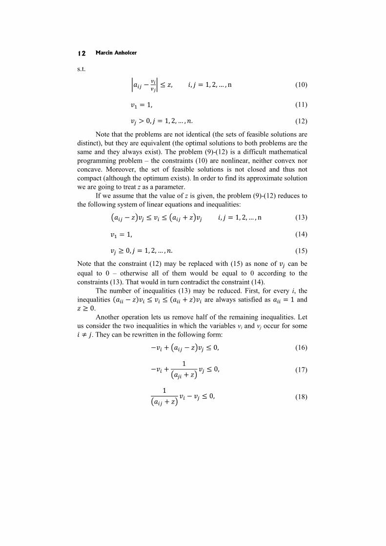
s.t. − ≤ , , = 1, 2, … , n (10)
= 1, (11)> 0, = 1, 2, … , . (12)
Note that the problems are not identical (the sets of feasible solutions are distinct), but they are equivalent (the optimal solutions to both problems are the same and they always exist). The problem (9)-(12) is a difficult mathematical programming problem – the constraints (10) are nonlinear, neither convex nor concave. Moreover, the set of feasible solutions is not closed and thus not compact (although the optimum exists). In order to find its approximate solution we are going to treat z as a parameter.
If we assume that the value of z is given, the problem (9)-(12) reduces to the following system of linear equations and inequalities: − ≤ ≤ + , = 1, 2, … , n (13)= 1, (14)≥ 0, = 1, 2, … , . (15)
Note that the constraint (12) may be replaced with (15) as none of can be equal to 0 – otherwise all of them would be equal to 0 according to the constraints (13). That would in turn contradict the constraint (14).
The number of inequalities (13) may be reduced. First, for every i, the inequalities ( − ) ≤ ≤ ( + ) are always satisfied as = 1 and ≥ 0.
Another operation lets us remove half of the remaining inequalities. Let us consider the two inequalities in which the variables vi and vj occur for some ≠ . They can be rewritten in the following form: − + − ≤ 0, (16)
− + 1+ ≤ 0, (17)
1+ − ≤ 0, (18)
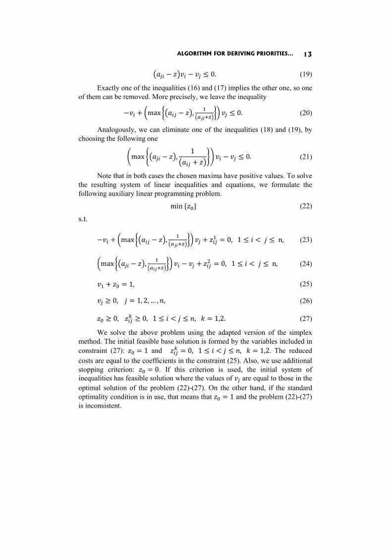
ALGORITHM FOR DERIVING PRIORITIES... 13− − ≤ 0. (19)
Exactly one of the inequalities (16) and (17) implies the other one, so one of them can be removed. More precisely, we leave the inequality − + max − , ≤ 0. (20)
Analogously, we can eliminate one of the inequalities (18) and (19), by choosing the following one max − , 1+ − ≤ 0. (21)
Note that in both cases the chosen maxima have positive values. To solve the resulting system of linear inequalities and equations, we formulate the following auxiliary linear programming problem. min { } (22)
s.t.
− + max − , + = 0, 1 ≤ < ≤ n, (23)
max − , − + = 0, 1 ≤ < ≤ n, (24)
+ = 1, (25)≥ 0, = 1, 2, … , , (26)≥ 0, ≥ 0, 1 ≤ < ≤ , = 1,2. (27)
We solve the above problem using the adapted version of the simplex method. The initial feasible base solution is formed by the variables included in constraint (27): = 1 and = 0, 1 ≤ < ≤ , = 1,2. The reduced costs are equal to the coefficients in the constraint (25). Also, we use additional stopping criterion: = 0. If this criterion is used, the initial system of inequalities has feasible solution where the values of are equal to those in the optimal solution of the problem (22)-(27). On the other hand, if the standard optimality condition is in use, that means that = 1 and the problem (22)-(27) is inconsistent.
Marcin Anholcer 14
Note also that if the feasible solution exists for some value of = ⋆, then it is also the solution for every value ≥ ⋆. That means also that if the system (13)-(15) is inconsistent for some value of = ⋆, then it is also inconsistent for every ≤ ⋆. This leads us to the following algorithm, where the starting point is generated by the geometric means of rows of A.
Algorithm 1
1. Assume the accuracy level > 0. Let ⋆ = ∏ and = ⋆⋆ for = 1, 2, … , . Let = = ( , ) and = 0. Proceed to step 2. 2. If − < then STOP. The vector v is the desired approximation
of the weight vector w. Otherwise go to step 3. 3. Set ≔ ( ). Solve the problem (22)-(27). If = 0, save the new
value of v and set : = . Otherwise do not change the value of v and set : = , ≔ . Go back to step 2.
In every step of the algorithm the value of − decreases twice, so in the finite number of iterations we obtain the approximation of the optimal solution (more precisely, if ⋆ denotes the initial value of , then the algorithm stops after log ⋆
steps).
3. Numerical example
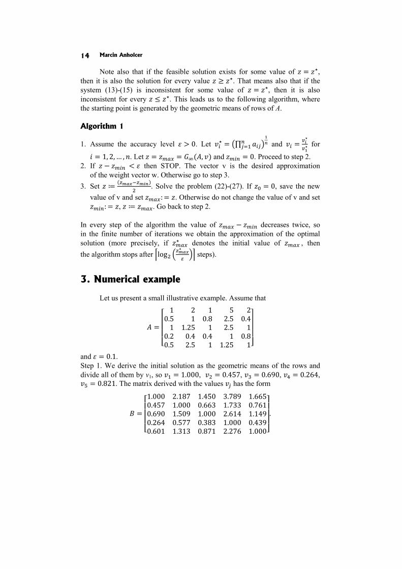
Let us present a small illustrative example. Assume that
= 1 2 1 5 20.5 1 0.8 2.5 0.41 1.25 1 2.5 10.2 0.4 0.4 1 0.80.5 2.5 1 1.25 1
and = 0.1. Step 1. We derive the initial solution as the geometric means of the rows and divide all of them by v1, so = 1.000, = 0.457, = 0.690, = 0.264, = 0.821. The matrix derived with the values has the form
= 1.000 2.187 1.450 3.789 1.6650.457 1.000 0.663 1.733 0.7610.690 1.509 1.000 2.614 1.1490.264 0.577 0.383 1.000 0.4390.601 1.313 0.871 2.276 1.000 .
ALGORITHM FOR DERIVING PRIORITIES... 15
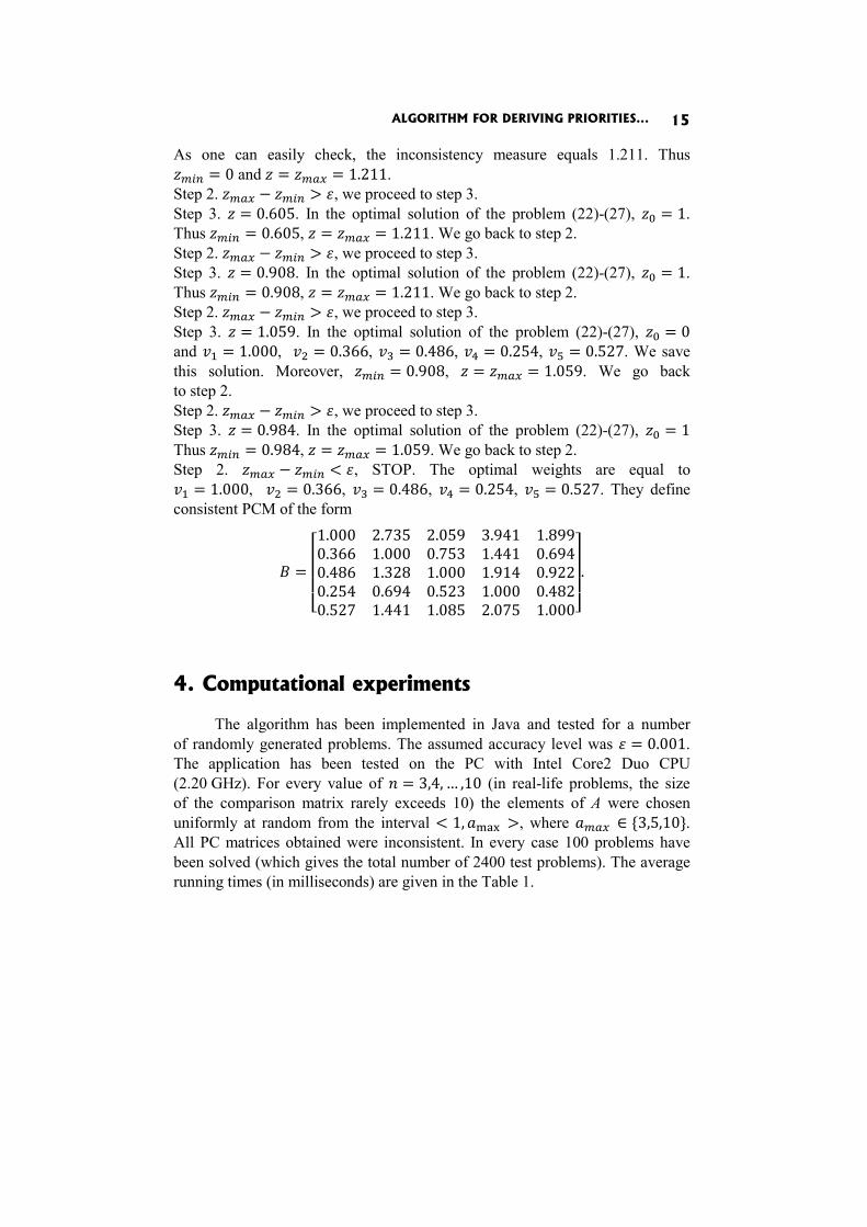
As one can easily check, the inconsistency measure equals 1.211. Thus = 0 and = = 1.211. Step 2. − > , we proceed to step 3. Step 3. = 0.605. In the optimal solution of the problem (22)-(27), = 1. Thus = 0.605, = = 1.211. We go back to step 2. Step 2. − > , we proceed to step 3. Step 3. = 0.908. In the optimal solution of the problem (22)-(27), = 1. Thus = 0.908, = = 1.211. We go back to step 2. Step 2. − > , we proceed to step 3. Step 3. = 1.059. In the optimal solution of the problem (22)-(27), = 0 and = 1.000, = 0.366, = 0.486, = 0.254, = 0.527. We save this solution. Moreover, = 0.908, = = 1.059. We go back to step 2. Step 2. − > , we proceed to step 3. Step 3. = 0.984. In the optimal solution of the problem (22)-(27), = 1 Thus = 0.984, = = 1.059. We go back to step 2. Step 2. − < , STOP. The optimal weights are equal to = 1.000, = 0.366, = 0.486, = 0.254, = 0.527. They define consistent PCM of the form
= 1.000 2.735 2.059 3.941 1.8990.366 1.000 0.753 1.441 0.6940.486 1.328 1.000 1.914 0.9220.254 0.694 0.523 1.000 0.4820.527 1.441 1.085 2.075 1.000 .
4. Computational experiments
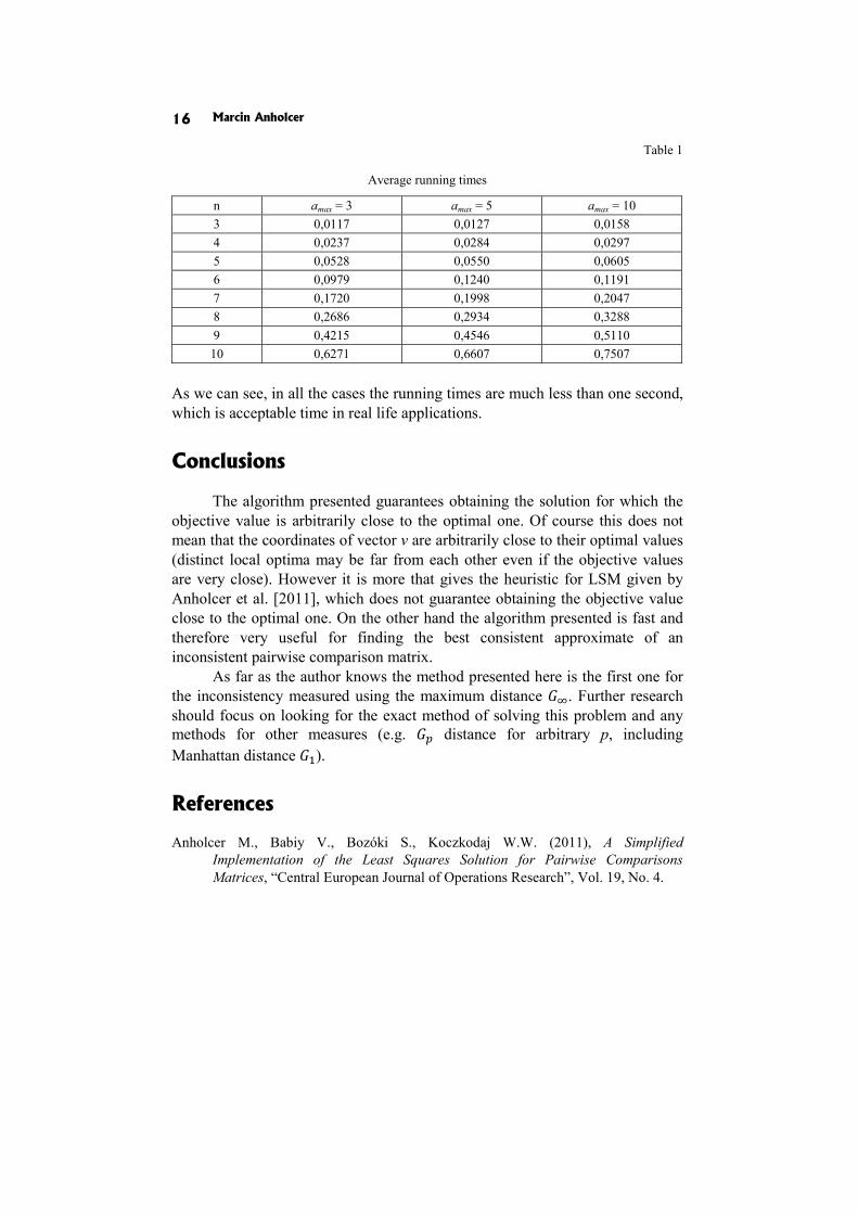
The algorithm has been implemented in Java and tested for a number of randomly generated problems. The assumed accuracy level was = 0.001. The application has been tested on the PC with Intel Core2 Duo CPU (2.20 GHz). For every value of = 3,4, … ,10 (in real-life problems, the size of the comparison matrix rarely exceeds 10) the elements of A were chosen uniformly at random from the interval < 1, >, where ∈ {3,5,10}. All PC matrices obtained were inconsistent. In every case 100 problems have been solved (which gives the total number of 2400 test problems). The average running times (in milliseconds) are given in the Table 1.
Marcin Anholcer 16
Table 1
Average running times
n amax = 3 amax = 5 amax = 10 3 0,0117 0,0127 0,0158 4 0,0237 0,0284 0,0297 5 0,0528 0,0550 0,0605 6 0,0979 0,1240 0,1191 7 0,1720 0,1998 0,2047 8 0,2686 0,2934 0,3288 9 0,4215 0,4546 0,5110 10 0,6271 0,6607 0,7507
As we can see, in all the cases the running times are much less than one second, which is acceptable time in real life applications.
Conclusions
The algorithm presented guarantees obtaining the solution for which the objective value is arbitrarily close to the optimal one. Of course this does not mean that the coordinates of vector v are arbitrarily close to their optimal values (distinct local optima may be far from each other even if the objective values are very close). However it is more that gives the heuristic for LSM given by Anholcer et al. [2011], which does not guarantee obtaining the objective value close to the optimal one. On the other hand the algorithm presented is fast and therefore very useful for finding the best consistent approximate of an inconsistent pairwise comparison matrix.
As far as the author knows the method presented here is the first one for the inconsistency measured using the maximum distance . Further research should focus on looking for the exact method of solving this problem and any methods for other measures (e.g. distance for arbitrary p, including Manhattan distance ).
References
Anholcer M., Babiy V., Bozóki S., Koczkodaj W.W. (2011), A Simplified Implementation of the Least Squares Solution for Pairwise Comparisons Matrices, “Central European Journal of Operations Research”, Vol. 19, No. 4.
ALGORITHM FOR DERIVING PRIORITIES... 17
Bozóki S. (2008), Solution of the Least Squares Method Problem of Pairwise Comparison Matrices, “Central European Journal of Operations Research”, No. 16.
Bozóki S., Rapcsàk T. (2008), On Saaty’s and Koczkodaj’s Inconsistencies of Pairwise Comparison Matrices, “Journal of Global Optimization”, No. 42.
Chu A.T.W., Kalaba R.E., Spingarn K. (1979), A Comparison of Two Method for Determining the Weights of Belonging to Fuzzy Sets, “Journal of Optimization Theory and Applications”, No. 27(4).
Erkut E., Tarimcilar M. (1991), On Sensitivity Analysis in the Analytic Hierarchy Process, “IMA Journal of Mathematics Applied in Business & Industry”, No. 3.
Fedrizzi M., Giove S. (2007), Incomplete Pairwise Comparison and Consistency Optimization, “European Journal of Operational Research”, No. 183.
Fülöp J., Koczkodaj W.W., Szarek S.J. (2010), A Different Perspective on a Scale for Pairwise Comparisons, Transactions on CCII, LNCS 6220.
Fülöp J. (2008), A Method for Approximating Pairwise Comparison Matrices by Consistent Matrices, “Journal of Global Optimization”, No. 42.
Hovanov N.V., Kolari J.W., Sokolov M.V. (2008), Deriving Weights from General Pairwise Comparison Matrices, “Mathematical Social Sciences”, No. 55.
Mogi W., Shinohara M. (2009), Optimum Priority Weight Estimation Method for Pairwise Comparison Matrix, ISAHP 2009 proceedings.
Saaty T.L. (1980), The Analytic Hierarchy Process, McGraw-Hill, New York.
Jakub Brzostowski
Tomasz Wachowicz
THE ANALYSIS OF NEGOTIATORS’ PREFERENCE CONSISTENCY IN INDIFFERENCE-SURFACE BASED SCORING SYSTEM
Abstract
In this paper we present a new method for analyzing the consistency of preferences of negotiators in building their scoring systems of negotiation offers. The method we propose can be used when the preferences are defined as general examples of full packages with the accompanying utility score, as it is done in the NegoManage negotiation support system in the conjoint analysis approach. During the preference elicitation stage the negotiators identify the indifference surfaces (or indifference sets) to which they also assign sample alternatives and scores. The verification of such the consistency of this assignment is based on the concept of the Jaccard index, that allows for measuring the similarity between fuzzy sets. Since we obtain a characteristics of equivalence sets in the form of probability distributions, which are further treated as fuzzy set membership functions, we can use the distribution characteristics to compute the Jaccard index for every pair of equivalence sets elicited from the negotiator. If these indexes are too high, the corresponding indifference sets should be reconsidered or integrated.
Keywords
Negotiation support, negotiation offers’ scoring system, preference elicitation, indifference sets, kernel density estimation.
Introduction
In the process of multiple criteria decision-making (MCDM) the decision makers have to cope with problems of comparing and evaluating very many (usually conflicting) criteria. Such decision-making processes involve, depending on the decision context of the problem, evaluation, prioritization or selection of alternatives. Among many MCDM methods the most popular
THE ANALYSIS OF NEGOTIATORS’ PREFERENCE CONSISTENCY... 19
are: simple additive weighting models (based on multiple attribute utility theory) − [Keeney and Raiffa 1993], AHP [Saaty 1980; Saaty and Alexander 1989], ELECTRE [Roy and Bouyssou 1993] and PROMETHE [Brans 1982]. The MAUT-based models constitute a scoring system allowing for ranking any alternative after the weights and marginal utilities have been elicited. This method fuses single attribute utilities with weights assigned to attributes and results in a final value of utility for the given alternative. The AHP method is based on pairwise comparisons of attributes and alternatives, and results in a ranking of the given alternatives. ELECTRE and PROMETHEE methods are based on an outranking concept and give as a result of analysis an ordering of the given alternatives. The literature review shows quite a lot of examples of using these methods in solving actual business-related decision making problems [see eds. Figuera et al. 2005; Omkarprasad and Sushil 2006; Behzadian et al. 2010]. In the negotiation context, however, it is a simple additive weighting (SAW) model that is most widely used for eliciting negotiators’ preferences. All the most popular negotiation support systems (NSSs) such as Inspire [Kersten and Noronha 1999], Negoist [Schoop et al. 2003] and SmartSettle [Thiessen and Soberg 2003] accomplish their decision support function by using the simple additive scoring model (sometimes hybridized with the conjoint analysis approach) for evaluating the negotiation template and building the scoring systems of the negotiation offers used in the actual negotiation phase for evaluation and analysis of the sequence of offers and counteroffers proposed by the parties as the negotiation contact proposals. But the recent negotiation experiments show that NSS users very often misinterpret the SAW scores and find it difficult to assign them to the negotiation options and issues [see Wachowicz and Kersten 2009; Paradis et al. 2010]. Therefore new mechanisms and systems are being built that apply preference elicitation approaches other than the SAW-based ones, such as NegoManage [Brzostowski and Wachowicz 2009, 2010] which allows to determine the scoring systems of negotiation offers deriving from the examples of offers that the negotiator specifies in the prenegotiation phase. The NegoManage system supports the negotiator in all phases of the negotiation process allowing not only for the preference elicitation but also for an exchange of offers and messages, tracking the negotiation history, negotiation profile identification and counterpart evaluation and selection. The preference elicitation engine is a key element of the system. The whole preference elicitation mechanism is based on the concept of the equivalence set that may be specified by the negotiator as a set of alternatives indifferent in terms of preferences. The negotiator also evaluates this set verbally by assigning to it a linguistic value of utility. The whole process of preference analysis requires
Jakub Brzostowski, Tomasz Wachowicz 20
of the negotiator the specification of the sequence of indifference sets with the corresponding utilities that are the basis for the scoring system of negotiation offers. After the scoring system has been prepared any alternative from the set of feasible alternatives (i.e. those defined in the template) can be evaluated in terms of utility assigned to this alternative. Since the preference analysis approach that we have applied in NegoManage system operates, similarly to the conjoint analysis approach, with complete offers and the corresponding score definitions (a full package must be specified and evaluated by the negotiators) we may face the problem of negotiator consistency in specifying different examples of offers and their scores. It may appear that two very similar packages are assigned to two separate indifference sets that differ much in terms of a linguistic utility evaluation or that the packages assigned to one indifference set differ too much to have assigned the same linguistic utility label. If so, we say that the problem of preference consistency occurs and consequently corrective actions need to be undertaken before the final scoring system is determined and used for the evaluation of offers in the actual negotiation phase.
In this paper we propose a simple mechanism for verifying the consistency of negotiators’ preferences that we apply in the NegoManage system. The preference consistency check is based on the concept of the Jaccard index allowing for measuring the similarity between fuzzy sets. Since the NegoManage preference elicitation approach allows to obtain the characteristics of equivalence sets in the form of probability distributions, we may further consider these functions as fuzzy sets membership functions and use the distribution characteristics to compute the Jaccard index for every pair of equivalence sets elicited from the negotiator. The Jaccard indexes measure similarity between the indifference sets defined by the negotiator. If for any two sets the Jaccard index is too high, it is recommended to reconsider these two indifference sets by analyzing both the examples of offers constituting these sets and the values of utility scores assigned to these sets. It may appear that it would be reasonable to join the sets or differentiate their original scores to obtain a more accurate final scoring system of negotiation offers.
The paper consist of four more sections. In Section 1 we introduce the general idea of eliciting preferences of negotiators in the NegoManage system. Then in Section 2 we give a deeper insight into the method of defining the preferences by means of indifference sets that we proposed earlier in the NegoManage NSS and discuss the issue of kernel density analysis required for determining the main characteristics of these sets. We present also briefly the major idea of the Jaccard index (Section 3) and the possibility of inter-change between the two alternative approaches to describing the indifference
THE ANALYSIS OF NEGOTIATORS’ PREFERENCE CONSISTENCY... 21
sets, i.e. probability-based and possibility-based. In Section 4 we show in detail an example of analyzing the preference of the negotiator and measuring its consistency using a very simple negotiation problem where the template consists of three negotiation issues only. We conclude the paper with some comments on the proposed mechanism of preference elicitation and consistency verification.
1. Preference representation in NegoManage system – Indifference sets and their characteristics
In the NegoManage system the negotiator defines preferences by specifying several sets of alternatives, called indifference sets (surfaces), and assigning a degree of utility to each surface. Each indifference set consists of the alternatives that the negotiator considers to be equally good. The degree of utility assigned to the surface is chosen from a linguistic (verbal) scale [see Yevseyeva et al. 2008]. The scale is build on two levels. The first-level scale consists of seven verbal terms. First, the negotiator assigns to the indifference set a level from this scale. The second-level scale allows for stating precisely the degree of utility; namely by choosing a degree between two neighboring terms from the first scale. The second scale consists also of seven verbal terms and leads to an increase in the precision of the utility specification. Each linguistic utility level has its numeric equivalent used during the scoring procedure. However, such sets consisting of alternatives representing a particular level of utility may not be sufficient for deriving a full scoring system of the negotiation offers. There are probably other alternatives that may also belong to this surface, that were not specified by the negotiators in the preference elicitation stage but could easily be built in the actual negotiation phase by changing proportionally the resolution levels of the subsequent negotiation issues (making implicitly trade-offs between the negotiation issues). Initially the negotiators may not have specified all the salient alternatives for a particular indifference set because of lack of time, haste or simply because they subjectively felt that a certain alternative is not important (conveys no important information) in the definition of this indifference surface. Therefore we need to remember that the alternatives that comprise the indifference surfaces are only examples of a particular utility. There are many other alternatives (especially in the continuous negotiation problems) that may also belong to each of these sets. However, the degree of belonging to a surface may be partial since for alternatives not classified directly by the negotiator we may never be sure of their belonging to this surface. To cope with this type
Jakub Brzostowski, Tomasz Wachowicz 22
of uncertainty we propose to model the level (or chance) of belonging to the surface by using the notion of probability. More precisely, we propose to build a characteristic of an indifference surface in the form of probability distribution. Such a function will assign to each alternative a level of belonging to the particular indifference surface.
After the surfaces have been specified and the utility degrees have been assigned, the NegoManage system performs its most important task, namely the computation of probability distributions for all specified surfaces that will be further used to build a global scoring system. The probability assigned to a particular point of the indifference surface can be interpreted as a chance of actual assignment of this point to the indifference set. To build the characteristic of a surface we use the following straightforward postulate:
The closer an alternative under consideration is located to the one that fully belongs to the indifference surface, the higher is the level of probability that we assign to this alternative.
In other words, for an alternative located in the neighborhood of a fully classified alternative we first compute the distance to the classified alternative and map it into a similarity degree. The similarity degree of the considered alternative to the fully classified alternative is regarded as the probability of belonging to the surface. Based on our postulate we propose to build peaks around the classified alternatives as a preliminary step of building the probability distribution. Such peaks may have a bell shape of the normal distribution curves, and such a peak shape is considered at the current stage of research. However, there are no substantial or experimentally proved reasons for using this type of probability distributions in our approach. We simply use the normal distribution functions as the most commonly used solution in the selection of the predefined shape of the probability function since we lack the relevant information that would allow us to use other types of probability distribution functions. In the next step such peaks are fused together to form an overall multi-modal distribution which is treated as the indifference surface’s characteristic together with utility levels assigned to the surfaces by the ne-gotiator. This information about each indifference set is a basis for determining the score of any feasible alternative under evaluation later on in the actual negotiation phase, when the negotiators face the problem of scoring the offers presented by their counterpart as the negotiation compromise proposals.
THE ANALYSIS OF NEGOTIATORS’ PREFERENCE CONSISTENCY... 23
2. Preference analysis in NegoManage system
Let us now look in detail at the formalism of the preference analysis approach implemented in the NegoManage system and described briefly in the previous section. Let us assume that the negotiator specifies a set of indifferent alternatives in the following form:
},,,{ 21 ni aaaRS K= (1)
where the indifference relationship holds between every pair of alternatives: ji aa ≈ .
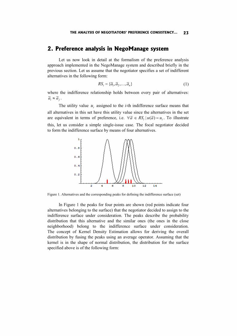
The utility value iu assigned to the i-th indifference surface means that all alternatives in this set have this utility value since the alternatives in the set are equivalent in terms of preference, i.e. ii uauRSa =∈∀ )(| . To illustrate this, let us consider a simple single-issue case. The focal negotiator decided to form the indifference surface by means of four alternatives.
Figure 1. Alternatives and the corresponding peaks for defining the indifference surface (set)
In Figure 1 the peaks for four points are shown (red points indicate four
alternatives belonging to the surface) that the negotiator decided to assign to the indifference surface under consideration. The peaks describe the probability distribution that this alternative and the similar ones (the ones in the close neighborhood) belong to the indifference surface under consideration. The concept of Kernel Density Estimation allows for deriving the overall distribution by fusing the peaks using an average operator. Assuming that the kernel is in the shape of normal distribution, the distribution for the surface specified above is of the following form:
Jakub Brzostowski, Tomasz Wachowicz 24
∑=
⎟⎟⎠
⎞⎜⎜⎝
⎛⎟⎠⎞
⎜⎝⎛ −
−=4
1
2
exp41)(
i
iRS d
mxd
xf . (2)
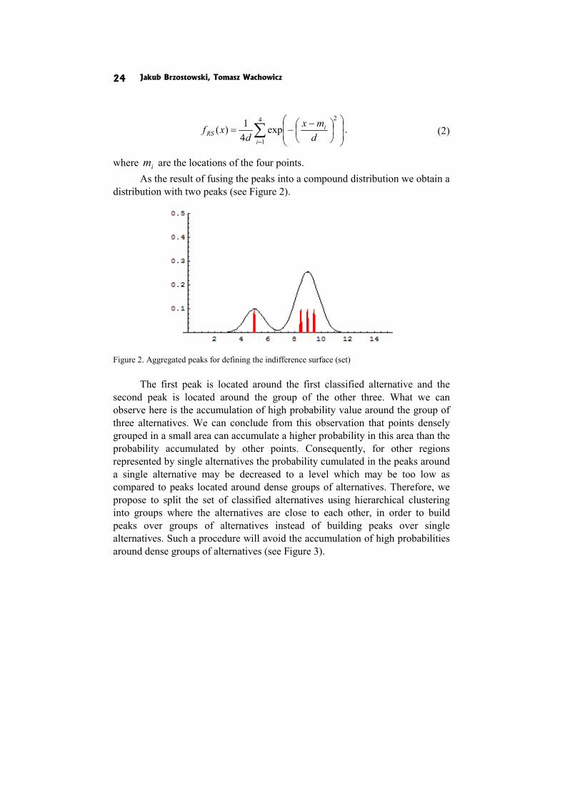
where im are the locations of the four points. As the result of fusing the peaks into a compound distribution we obtain a
distribution with two peaks (see Figure 2).
Figure 2. Aggregated peaks for defining the indifference surface (set)
The first peak is located around the first classified alternative and the
second peak is located around the group of the other three. What we can observe here is the accumulation of high probability value around the group of three alternatives. We can conclude from this observation that points densely grouped in a small area can accumulate a higher probability in this area than the probability accumulated by other points. Consequently, for other regions represented by single alternatives the probability cumulated in the peaks around a single alternative may be decreased to a level which may be too low as compared to peaks located around dense groups of alternatives. Therefore, we propose to split the set of classified alternatives using hierarchical clustering into groups where the alternatives are close to each other, in order to build peaks over groups of alternatives instead of building peaks over single alternatives. Such a procedure will avoid the accumulation of high probabilities around dense groups of alternatives (see Figure 3).

THE ANALYSIS OF NEGOTIATORS’ PREFERENCE CONSISTENCY... 25
Figure 3. Aggregated peaks for the alternatives grouped within the indifference surface (set)
In a general multi-issue negotiation problem the probability distributions
corresponding to the indifference surfaces are of multivariate form. Therefore, first we define the negotiation alternatives as follows. Every alternative a is described by a sequence of mappings mggg ,,, 21 K in the following way:
))(,),(),(( 21 agagaga mK= . (3)
where each mapping sg maps the alternative a into the numerical value of sth issue.
The simplest way to cluster the alternatives constituting the indifference set is to use hierarchical clustering [see Hartigan 1975; Hair and Black 1992]. The algorithm is agglomerative which means that at the beginning of the procedure each cluster consists of one alternative. In the next stages of the clustering algorithm the clusters are successively merged together. The number of clusters is decreasing while the size of clusters grows. The merging stops when the maximal distance between the alternatives inside the clusters reaches a selected level. As a result of this algorithm we obtain a split of the indifference surface. Given a split of the set iRS into k disjoint subsets
ikii MMM ,,, 21 K , the means for all subsets (clusters) are computed:
ikii mmm ,,, 21 K (for the computation of the mean we use simple average). The multi-modal distribution is built over the indifference surface consisting of kernels determined over subsets ijM [see Parzen 1962]. For the jth cluster of the ith indifference surface the multi-normal kernel distribution may be calculated:
Jakub Brzostowski, Tomasz Wachowicz 26
⎟⎠⎞
⎜⎝⎛ −Σ−
Σ= − )()'(
21exp
||)2(1)( 1
2/12/ ijijijij
kM mamaafij π
. (4)
where ijΣ is the covariance matrix. Let us assume that },,,{ 21 nij aaaM K= . For the estimation of the
covariance matrix we use the following estimator:
∑=
−−−
=Σn
lijlijlij mama
n 1
)')((1
1 . (5)
where the operator ' is the matrix transposition. Having the distributions
ijMf for all clusters ijM the final characteristics
in the form of a multi-modal distribution is built and has the following form:
∑=
=k
jMRS af
kaf
ijl1
)(1)( . (6)
The final scoring system consists of the sequence of indifference sets distributions together with its utility (defined in a linguistic form) assigned to the indifference set by the negotiator:
},,1{),( miuf iRSiK∈ . (7)
During the actual negotiation phase the scoring system is used to evaluate the chosen alternative a in the following way. First the degree of belonging to a particular indifference set is computed. In other words, the probability of belonging to a particular indifference set is computed:
},,1{)()()( miafapipiRSi K∈== . (8)
The degree of belonging )(api is computed for all indifference sets. As a result we obtain a discrete probability distribution over a set of indices
},,1{ mi K∈ indexing all indifference surfaces (indifference sets). The distribution )(ip tells us the degree of belonging of the given alternative to any indifference set. In the next step of computation we need to obtain the final utility for the alternative a . In other words, we look for the indifference set to which the alternative a belongs with the highest degree. However, the notion of belonging to a set is not binary here. The alternative may belong to many indifference sets with different values of belonging degree. Therefore, to obtain the indifference set index and the final utility of the alternative a we use the
THE ANALYSIS OF NEGOTIATORS’ PREFERENCE CONSISTENCY... 27
concept of von Neumann-Morgenstern expected utility [see Neumann and Morgenstern 1944]. The linguistic utility in NegoManage consists of two linguistic values ),( 21 ii νν describing the utility in terms of two integrated scales and these values correspond to numerical interval ],[ ii rl :
},,1{],[),( 21 mirlu iiiii K∈→= νν . (9)
These two boundary values of expected utility (lower and upper) are computed as follows:
∑=
⋅=n
iii lapaLEU
1
)()( , (10)
i
n
ii rapaUEU ⋅= ∑
=1
)()( . (11)
As a result we obtain a pair of utilities describing the final utility interval )](),([ aUEUaLEU that can be mapped back into linguistic utility to present
it to the user. The precise description of interval in numerical form can be used in further computation.
3. Preference consistency and Jaccard index
The consistency of the scoring system is a key issue in the NegoManage system. Since one set contains alternatives ranked with a different degree of utility and a different indifference set contains alternatives ranked with different degree of utility, two difference sets with different utility values should not overlap (should be disjoint). If an alternative belonged to different indifference surfaces, it would mean that different levels of utility have been assigned to the same alternative. Therefore, we assume that the preference structure is fully consistent if all indifference surfaces are disjoint. However, if there is a partial overlap of two indifference surfaces, namely some alternatives partially belong to both surfaces, then a measure needs to be defined indicating the extent to which the condition of separation of two surfaces is violated. This extent is indicated in the simplest possible way by the number of alternatives belonging to both surfaces. However, we need to normalize this value to make the measure of inconsistency universal. The normalization is obtained by dividing the cardinality of the intersection of two surfaces by the cardinality of the union of these surfaces. If the intersection of two surfaces is non-empty, we will measure the preference inconsistency using the Jaccard index described above, given by the following formula:
Jakub Brzostowski, Tomasz Wachowicz 28
)()(),(
BAmBAmBAJ
∪∩
= . (12)
where m is the cardinality of a set. In the NegoManage system we have at our disposal the characteristics
of surfaces given by probability distributions. We use the concept of probability to describe the degree of belonging of an alternative to the indifference surface. However, this interpretation can be also used if we want to describe the indifference surface in the form of a fuzzy set, namely with the membership degree stating the extent to which an alternative is included in the fuzzy indifference surface. Unfortunately, from a formal point of view, the probability distributions cannot be directly treated as membership functions of a fuzzy surface. One of the reasons for this is the normalization axiom defined in different way for a probability distribution and a possibility distribution (a fuzzy set concept used to describe the plausibility of belonging to the indifference surface in our application context). Namely, the normalization condition for the probability distributions means that the probabilities of all alternatives sum up to 1, and in the case of a possibility distribution the function reaches 1 for some alternative (which is the maximal distribution value). The following formula is an extension of the concept of the Jaccard index for fuzzy sets or possibility distributions:
))(),(max(max))(),(min(max
)()(),(
uuuu
BAmBAmBAJ
BAu
BAu
μμμμ
Ω∈
Ω∈=∪∩
= . (13)
where Ω is the space of all feasible alternatives, and BA μμ , are the membership functions of the sets A and B.
To apply the fuzzy Jaccard coefficient in our particular application context, first we need to convert the surface characteristics given in the forms of probability distributions into possibility distributions. Such conversions have been proposed by Dubois et al. [2004]. The most important axiom distinguishing the possibility measures from probability measures is:
}),(sup{)( AxxAXA ∈=Π⊆∀ π . (14)
THE ANALYSIS OF NEGOTIATORS’ PREFERENCE CONSISTENCY... 29
As we can see, this axiom involves the supremum operation instead of Riemann integration as it is done in the case of probability measures
∫=⊆∀A
dxxpAPXA )()( . (15)
Probability and possibility measures capture different facets of uncertainty. In the case of two disjoint subsets measured using probability measure, the measure of their union is equal to the sum of their measures. In the case of possibility measures the measure of union of disjoint subsets is the supremum (maximum in the case of finite sets). But some linkages between these two approaches may be distinguished (Dubois et al. 2004):
As it turns out, a numerical possibility measure, restricted to measurable subsets, can also be viewed as an upper probability function [Dubois and Prade 1992]. Formally, such a real-valued possibility measure P is equivalent to the family P(P) of probability measures such that
)}()(,,{)( AAPmeasurableAPP Π≤∀=Π
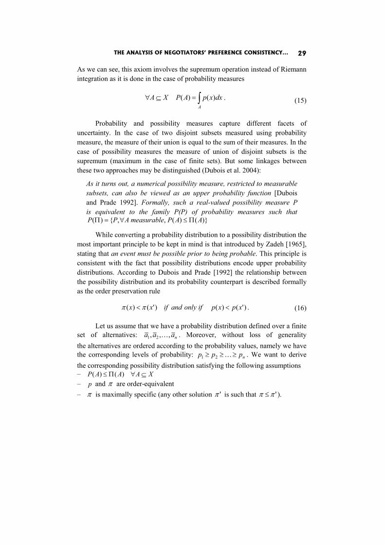
While converting a probability distribution to a possibility distribution the most important principle to be kept in mind is that introduced by Zadeh [1965], stating that an event must be possible prior to being probable. This principle is consistent with the fact that possibility distributions encode upper probability distributions. According to Dubois and Prade [1992] the relationship between the possibility distribution and its probability counterpart is described formally as the order preservation rule
)'()()'()( xpxpifonlyandifxx << ππ . (16)
Let us assume that we have a probability distribution defined over a finite set of alternatives: naaa ,,, 21 K . Moreover, without loss of generality the alternatives are ordered according to the probability values, namely we have the corresponding levels of probability: nppp ≥≥≥ K21 . We want to derive the corresponding possibility distribution satisfying the following assumptions – XAAAP ⊆∀Π≤ )()( – p and π are order-equivalent – π is maximally specific (any other solution 'π is such that 'ππ ≤ ).
Jakub Brzostowski, Tomasz Wachowicz 30
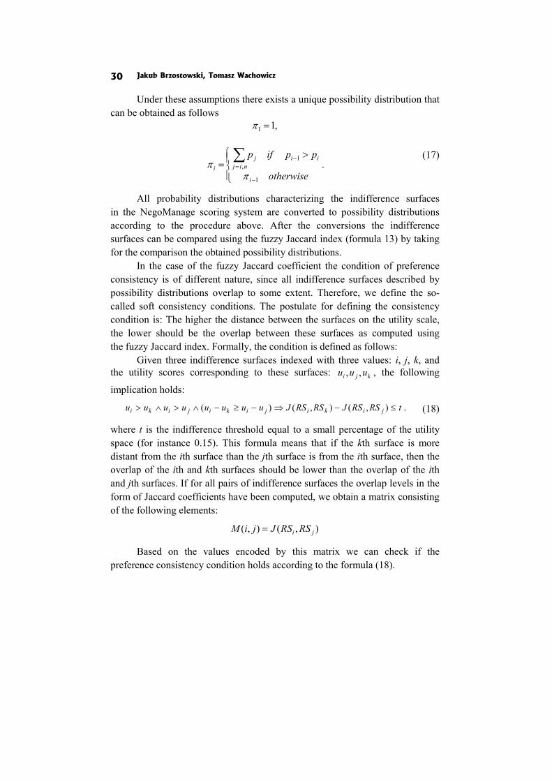
Under these assumptions there exists a unique possibility distribution that can be obtained as follows
,11 =π
⎪⎩
⎪⎨⎧ >
=−
−=∑
otherwise
ppifp
i
iinij
ji
1
1,
ππ .
(17)
All probability distributions characterizing the indifference surfaces in the NegoManage scoring system are converted to possibility distributions according to the procedure above. After the conversions the indifference surfaces can be compared using the fuzzy Jaccard index (formula 13) by taking for the comparison the obtained possibility distributions.
In the case of the fuzzy Jaccard coefficient the condition of preference consistency is of different nature, since all indifference surfaces described by possibility distributions overlap to some extent. Therefore, we define the so-called soft consistency conditions. The postulate for defining the consistency condition is: The higher the distance between the surfaces on the utility scale, the lower should be the overlap between these surfaces as computed using the fuzzy Jaccard index. Formally, the condition is defined as follows:
Given three indifference surfaces indexed with three values: i, j, k, and the utility scores corresponding to these surfaces: kji uuu ,, , the following
implication holds:
tRSRSJRSRSJuuuuuuuu jikijikijiki ≤−⇒−≥−∧>∧> ),(),()( . (18)
where t is the indifference threshold equal to a small percentage of the utility space (for instance 0.15). This formula means that if the kth surface is more distant from the ith surface than the jth surface is from the ith surface, then the overlap of the ith and kth surfaces should be lower than the overlap of the ith and jth surfaces. If for all pairs of indifference surfaces the overlap levels in the form of Jaccard coefficients have been computed, we obtain a matrix consisting of the following elements:
),(),( ji RSRSJjiM =
Based on the values encoded by this matrix we can check if the preference consistency condition holds according to the formula (18).
THE ANALYSIS OF NEGOTIATORS’ PREFERENCE CONSISTENCY... 31
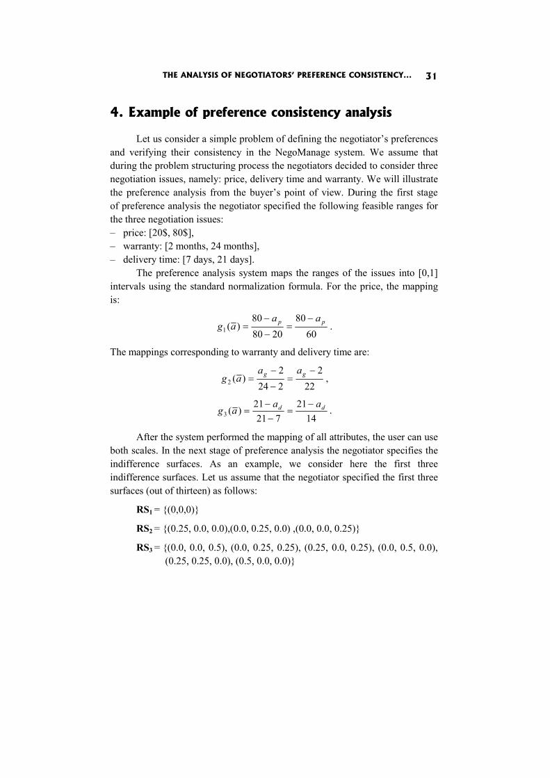
4. Example of preference consistency analysis
Let us consider a simple problem of defining the negotiator’s preferences and verifying their consistency in the NegoManage system. We assume that during the problem structuring process the negotiators decided to consider three negotiation issues, namely: price, delivery time and warranty. We will illustrate the preference analysis from the buyer’s point of view. During the first stage of preference analysis the negotiator specified the following feasible ranges for the three negotiation issues: – price: [20$, 80$], – warranty: [2 months, 24 months], – delivery time: [7 days, 21 days].
The preference analysis system maps the ranges of the issues into [0,1] intervals using the standard normalization formula. For the price, the mapping is:
6080
208080
)(1pp aa
ag−
=−
−= .
The mappings corresponding to warranty and delivery time are:
222
2242
)(2
−=
−
−= gg aa
ag ,
1421
72121
)(3dd aa
ag−
=−
−= .
After the system performed the mapping of all attributes, the user can use both scales. In the next stage of preference analysis the negotiator specifies the indifference surfaces. As an example, we consider here the first three indifference surfaces. Let us assume that the negotiator specified the first three surfaces (out of thirteen) as follows:
RS1 = {(0,0,0)}
RS2 = {(0.25, 0.0, 0.0),(0.0, 0.25, 0.0) ,(0.0, 0.0, 0.25)}
RS3 = {(0.0, 0.0, 0.5), (0.0, 0.25, 0.25), (0.25, 0.0, 0.25), (0.0, 0.5, 0.0), (0.25, 0.25, 0.0), (0.5, 0.0, 0.0)}
Jakub Brzostowski, Tomasz Wachowicz 32
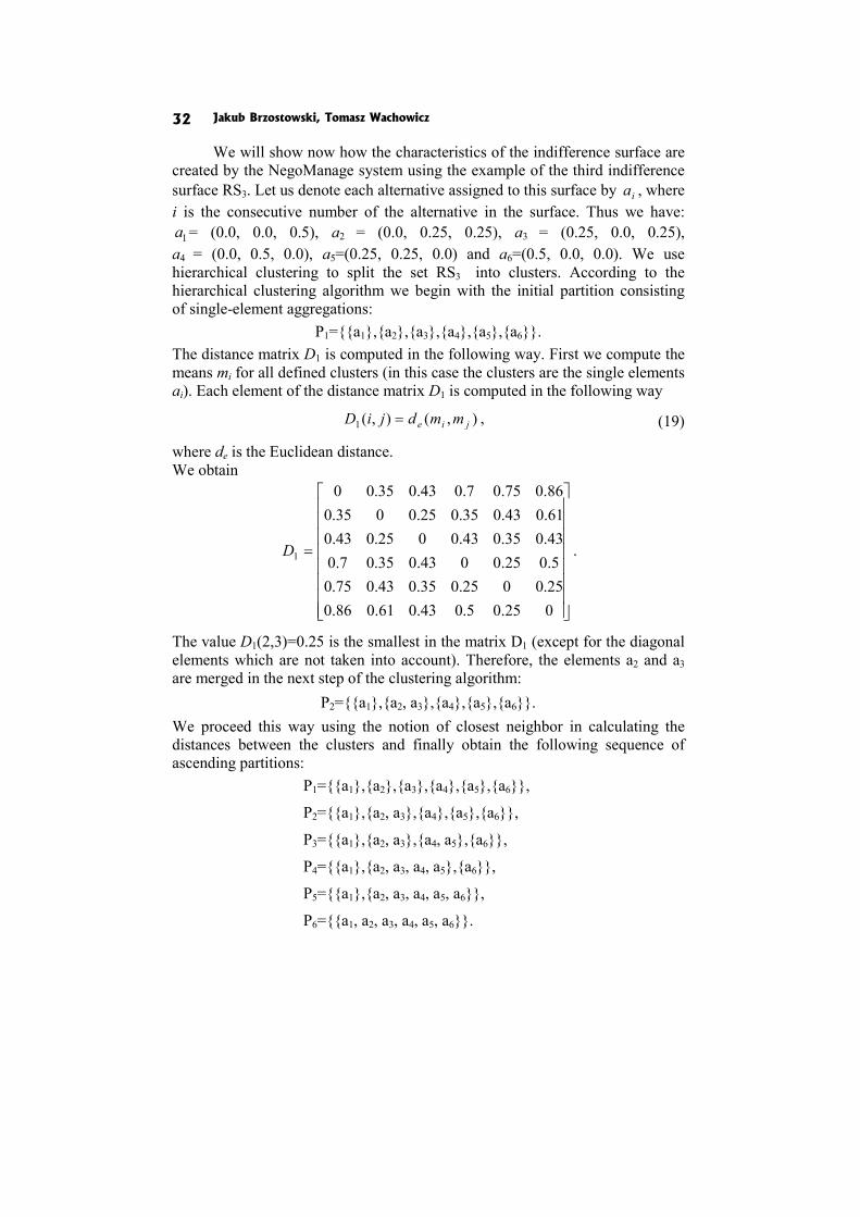
We will show now how the characteristics of the indifference surface are created by the NegoManage system using the example of the third indifference surface RS3. Let us denote each alternative assigned to this surface by ia , where i is the consecutive number of the alternative in the surface. Thus we have:
1a = (0.0, 0.0, 0.5), a2 = (0.0, 0.25, 0.25), a3 = (0.25, 0.0, 0.25), a4 = (0.0, 0.5, 0.0), a5=(0.25, 0.25, 0.0) and a6=(0.5, 0.0, 0.0). We use hierarchical clustering to split the set RS3 into clusters. According to the hierarchical clustering algorithm we begin with the initial partition consisting of single-element aggregations:
P1={{a1},{a2},{a3},{a4},{a5},{a6}}. The distance matrix D1 is computed in the following way. First we compute the means mi for all defined clusters (in this case the clusters are the single elements ai). Each element of the distance matrix D1 is computed in the following way
),(),(1 jie mmdjiD = , (19)
where de is the Euclidean distance. We obtain
⎥⎥⎥⎥⎥⎥⎥⎥
⎦
⎤
⎢⎢⎢⎢⎢⎢⎢⎢
⎣
⎡
=
025.05.043.061.086.025.0025.035.043.075.05.025.0043.035.07.043.035.043.0025.043.061.043.035.025.0035.086.075.07.043.035.00
1D .
The value D1(2,3)=0.25 is the smallest in the matrix D1 (except for the diagonal elements which are not taken into account). Therefore, the elements a2 and a3 are merged in the next step of the clustering algorithm:
P2={{a1},{a2, a3},{a4},{a5},{a6}}. We proceed this way using the notion of closest neighbor in calculating the distances between the clusters and finally obtain the following sequence of ascending partitions:
P1={{a1},{a2},{a3},{a4},{a5},{a6}},
P2={{a1},{a2, a3},{a4},{a5},{a6}},
P3={{a1},{a2, a3},{a4, a5},{a6}},
P4={{a1},{a2, a3, a4, a5},{a6}},
P5={{a1},{a2, a3, a4, a5, a6}},
P6={{a1, a2, a3, a4, a5, a6}}.
THE ANALYSIS OF NEGOTIATORS’ PREFERENCE CONSISTENCY... 33
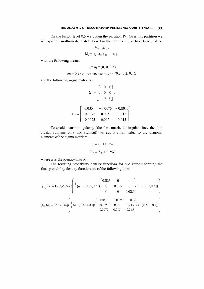
On the fusion level 0.5 we obtain the partition P5 . Over this partition we will span the multi-modal distribution. For the partition P5 we have two clusters:
M1={a1},
M2={a2, a3, a4, a5, a6},
with the following means:
m1 = a1 = (0, 0, 0.5),
m2 = 0.2 (a2 +a3 +a4 +a5 +a6) = (0.2, 0.2, 0.1).
and the following sigma matrices:
⎥⎥⎥
⎦
⎤
⎢⎢⎢
⎣
⎡=Σ
000000000
1 ,
⎥⎥⎥
⎦
⎤
⎢⎢⎢
⎣
⎡
−−
−−=Σ
015.0015.00075.0015.0015.00075.00075.00075.0035.0
2 .
To avoid matrix singularity (the first matrix is singular since the first cluster contains only one element) we add a small value to the diagonal elements of the sigma matrices:
E25.011 +Σ=Σ
E25.022 +Σ=Σ
where E is the identity matrix. The resulting probability density functions for two kernels forming the
final probability density function are of the following form:
⎟⎟⎟
⎠
⎞
⎜⎜⎜
⎝
⎛−
⎥⎥⎥
⎦
⎤
⎢⎢⎢
⎣
⎡−= ])5.0,5.0,0[(
025.0000025.0000025.0
])'5.0,5.0,0[(21exp7389.12)(
1aaafM
⎟⎟⎟
⎠
⎞
⎜⎜⎜
⎝
⎛−
⎥⎥⎥
⎦
⎤
⎢⎢⎢
⎣
⎡
−−
−−−= ])1.0,1.0,2.0[(
265.0015.00075.0015.004.0075.0075.00075.006.0
])'1.0,1.0,2.0[(21exp46301.6)(
2aaafM
Jakub Brzostowski, Tomasz Wachowicz 34
The final function for the indifference set RS3 is represented by:
))()((21)(
213afafaf MMRS += .
Similarly, the probability density functions are calculated for all thirteen remaining equivalence sets.
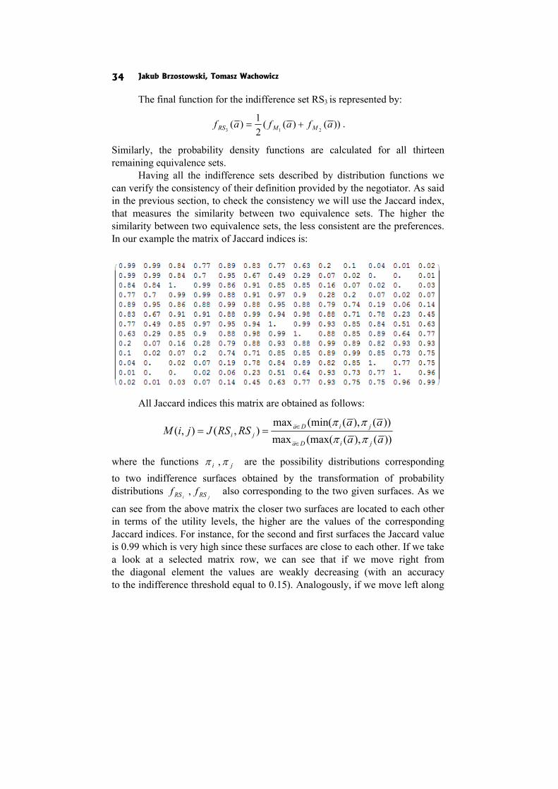
Having all the indifference sets described by distribution functions we can verify the consistency of their definition provided by the negotiator. As said in the previous section, to check the consistency we will use the Jaccard index, that measures the similarity between two equivalence sets. The higher the similarity between two equivalence sets, the less consistent are the preferences. In our example the matrix of Jaccard indices is:
All Jaccard indices this matrix are obtained as follows:
))(),((max(max))(),((min(max
),(),(aaaa
RSRSJjiMjiDa
jiDaji ππ
ππ
∈
∈==
where the functions ji ππ , are the possibility distributions corresponding to two indifference surfaces obtained by the transformation of probability distributions
ji RSRS ff , also corresponding to the two given surfaces. As we
can see from the above matrix the closer two surfaces are located to each other in terms of the utility levels, the higher are the values of the corresponding Jaccard indices. For instance, for the second and first surfaces the Jaccard value is 0.99 which is very high since these surfaces are close to each other. If we take a look at a selected matrix row, we can see that if we move right from the diagonal element the values are weakly decreasing (with an accuracy to the indifference threshold equal to 0.15). Analogously, if we move left along
THE ANALYSIS OF NEGOTIATORS’ PREFERENCE CONSISTENCY... 35
the row from the diagonal element the values are also weakly decreasing (with an accuracy to the indifference threshold equal to 0.15). The same observation holds if we move along a column up or down from the diagonal element. In this example we have defined surfaces preserving the preference consistency condition in terms of crisp definitions of the Jaccard index. If two indifference surfaces in a crisp form are disjoint (consistency condition holds – Jaccard index is equal to 0) its fuzzy counterparts (fuzzy surfaces) should in result have low level of overlap when the fuzzy Jaccard index is used for the comparison of surfaces (fuzzy Jaccard index should be low).
Conclusions
In this paper we presented a straightforward method for checking the negotiator’s preference consistency for the preference elicitation method based on the notion of indifference sets, applied in the NegoManage system, that we have built and developed beforehand [see Brzostowski and Wachowicz 2009, 2010]. It seems vital to verify whether the negotiator defines preferences in a coherent and consistent way in every decision problem, but especially when the preference elicitation process has a decompositional character, i.e. the preferences are derived from the examples of the predefined complete packages and evaluated by the negotiator in the prenegotiation phase. In this approach it may very often appear that while defining the examples, the negotiator builds two very similar examples of negotiation offers but assigns them to two indifferent sets with different utility scores. If such a situation occurs, the scoring system of negotiation offers derived from the predefined examples appears imprecise and may result in the false scorings determined for the negotiation offers under evaluation in the actual negotiation phase. If so, the negotiator may feel that the whole scoring system is not adequate to her/his subjective and intrinsic preferences that she/he tried to define in prenegotiation. To avoid such a situation we recommend to check the consistency of pre-ferences just after the definition of the examples of offers and the determination of the characteristics of indifference sets given in the form of distribution functions. We decided to use the simplest possible solution, which is to apply the Jaccard index. Given two sets, the Jaccard index compares the number of alternatives that may be assigned to both sets with the number of alternatives assigned to each set separately. However, while describing the indifference sets we operate with probability distribution functions, therefore we tried to give a rationale to move to the concept of possibility and used the Jaccard index formula defined for the fuzzy sets or possibility distributions. This simple
Jakub Brzostowski, Tomasz Wachowicz 36
mechanism allows us to find the sets that are too similar and ask the negotiator to revise their definitions. If two similar indifference sets are identified, the negotiator may change their forms by moving or eliminating some sample offers within the sets. She/he may also decide to join these two sets if necessary and assign to them a new value of the linguistic utility. After the negotiator’s revision the consistency checkup is conducted once again to verify the impact of these changes on the form and quality of the new scoring system of negotiation offers.
Acknowledgements
This research is supported by the grant of Polish Ministry of Science and Higher Education (N N111 362337).
References
Behzadian M., Kazemzadeh R.B., Albadvi A., Aghdasi M. (2010), PROMETHEE: A Comprehensive Literature Review on Methodologies and Applications, “European Journal of Operational Research”, No. 200(1).
Brans J. (1982), L'ingéniérie de la décision. Elaboration d'instruments d'aide à la décision. Méthode PROMETHEE, Universite Laval, Québec.
Brzostowski J., Wachowicz T. (2009), Conceptual Model of eNS For Supporting Preference Elicitation and Counterpart Analysis, [in:] Proceedings of GDN 2009: An International Conference on Group Decision and Negotiation, eds. D.M. Kilgour, Q. Wang, Wilfried Laurier University, Waterloo.
Brzostowski J., Wachowicz T. (2010), Building Personality Profile Of Negotiator For Electronic Negotiations, [in:] Multiple Criteria Decision Making '09, eds. T. Trzaskalik, T. Wachowicz, The Publisher of The University of Economics, Katowice.
Dubois D., Prade H. (1992), When upper Probabilities are Possibility Measures, “Fuzzy Sets and Systems”, No. 49.
Dubois D., Foulloy L., Mauris G., Prade H. (2004), Probability-possibility Transfor-mations, Triangular Fuzzy Sets and Probabilistic Inequalities, “Reliable Com-puting”, No. 10.
Figuera J., Greco S., Ehrgott M. (eds.), 2005, Multiple Criteria Decision Analysis. State of the Art Surveys, Springer Science + Business Media, Boston.
Hair J.F., Black B. (1992), Multivariate Data Analysis, Macmillan, New York. Hartigan J. (1975), Clustering Algorithms, Wiley.
THE ANALYSIS OF NEGOTIATORS’ PREFERENCE CONSISTENCY... 37
Keeney R., Raiffa H. (1993), Decisions with Multiple Objectives: Preferences and Value Tradeoffs, Cambridge University Press, New York.
Kersten G.E, Noronha S.J. (1999), WWW-based Negotiation Support: Design, Implementation and Use, “Decision Support Systems”, No. 25(2).
Neumann J. von, Morgenstern O. (1944), Theory of Games and Economic Behavior, Princeton Univerosty Press, Princeton.
Omkarprasad S.V., Sushil K. (2006), Analytic Hierarchy Process: An Overview of Applications, “European Journal of Operational Research”, No. 169(1).
Paradis N., Gettinger J., Lai H., Surboeck M., Wachowicz T. (2010), E-Negotiations via Inspire 2.0: The System, Users, Management and Projects, [in:] Group Decision and Negotiations 2010. Proceedings. The Center for Collaboration Science, ed. G.J. de Vreede, University of Nebraska at Omaha.
Parzen E. (1962), On Estimation of a Probability Density Function and Mode, “Ann. Math. Stat.” 33.
Roy B., Bouyssou D., (1993), Aide multicritere a la decision: Methodes et cas, Economica, Paris.
Saaty T.L., Alexander J.M. (1989), Conflict Resolution: The Analytic Hierarchy Approach, Praeger, New York.
Saaty T. (1980), The Analytic Hierarchy Process, McGraw Hill, New York. Schoop M., Jertila A., List T. (2003), Negoisst: A Negotiation Support System for
Electronic Business-to Business Negotiations in Ecommerce, “Data and Know-ledge Engeneering”, No. 47.
Thiessen E.M., Soberg A. (2003), Smartsettle Described with the Montreal Taxonomy, “Group Decision and Negotiation”, 12.
Wachowicz T., Kersten G.E. (2009), Zachowania i decyzje negocjacyjne uczestników negocjacji elektronicznych, [w:] Człowiek i jego decyzje, tom 2, red. K.A. Kło-siński, A. Biela, Wydawnictwo KUL, Lublin.
Zadeh Z.A. (1965), Fuzzy Sets, “Information and Control”, No. 8. Yevseyeva I., Miettinen K., Räsänen P. (2008), Verbal Ordinal Classification with
Multicriteria Decision Aiding, “European Journal of Operational Research”, No. 185.
Rafael Caballero
Francisca García Lopera
José Enrique Padilla García
Fátima Pérez
DEFAULT PREDICTION FOR VARIOUS NATIONAL ECONOMIES THROUGH SYNTHETIC INDICATORS
Abstract
In the current situation, involving a global economic crisis, national economies are under a high pressure. Greek and Irish bailouts have prompted many people to wonder about the economic situation in other countries. The global crisis is causing First World countries need help from institutions such as the IMF or the ECB. The goal of this paper is to analyze the risk that these countries have to be rescued by the economic institutions. In order to prepare this ranking, we are going to use two synthetic indicators. The first one is called Distance Principal Components (DPC) and the other one Goal Programming Synthetic Indicator (GPSI). We develop this indicator taking into account variables from both the public economy and the financial markets. Concerning the public economy, we use variables such as the public debt ratio and its total amount (% of GDP), public revenues, public deficit, real GDP growth and unemployment rate. We strongly believe that the soundness of an economy in the long-term depends on the behavior of these variables. Therefore, if they show a positive trend, other variables exposed to speculation in the financial markets should present a proper behavior as well. With this we mean two variables negotiated in the markets: debt risk premium and credit default swap levels.
This paper will bring easily understandable results that will let us know what the bankruptcy situation is in the rest of the countries analyzed.
Keywords
National Economies, Synthetic Indicators, GPSI indicator.
DEFAULT PREDICTION FOR VARIOUS NATIONAL ECONOMIES... 39
Introduction
In a world that is totally globalized, the situation of the worldwide economies is of increasing importance. After Greece's and Ireland's rescues by the European Institutions, there is a special worry about a new hypothetical bankruptcy in Europe.
The European Union (EU) has been able to deal with this problem until this moment. Taking into account that Greece's and Ireland's Gross Domestic Product (GDP) represented only around the 4% of the EU GDP in 2009, the problem was not too serious, so that EU institutions could solve it without any external help. In addition, the EU will only ask for help to the International Monetary Fund (IMF) if it is impossible to fix the situation within the EU. It makes no sense to create an Economic and Monetary Union if later they cannot solve their own problems. However, what if a powerful economy like Spain or Italy has to be rescued? Can the EU afford it? That is the reason why the current economic context has such a great importance. It is said that, if there is a new bailout, IMF funds would have to be used. In that case, what we know as 'Eurozone' would be over and we should reconsider the EU as something else than a simple 'geographical Union'.
Through this paper we try to quantify the risk countries have to be rescued. We have focused on important economies from the European Union and the rest of the world. Firstly, because what happens in the EU affects us directly, and secondly, because the non-European economies we have chosen are very powerful and, as we said before, in a globalized world we are strongly influenced by them, it must be said that many companies try to quantify the default risk countries. However, they build the index taking into account only the Credit Default Swap of a country [Kan and Pedersen 2011]. We believe that other variables have to be added to the index because the CDS value is fixed in the financial markets and it is a very volatile variable. The strengths and weaknesses of an economy lie mainly in the real economy. Credit default swaps have existed since the early 1990s. At the beginning they had a marginal role only in the economy. However, in 2003 there was a 'boom' and the market increased tremendously. We think that a variable that is always under negotiation and speculation cannot be a good indicator of the actual state of an economy.
We have chosen a sample of countries. Many of them belong to the Eurozone and EU27 but we also wanted to see how the index works in some countries which do not have the same political economy. We could have increased the number of countries as much as we had wanted but we strongly believe that 20 countries from different parts of the world suffice.
Rafael Caballero, Francisca García Lopera, José Enrique Padilla García, Fátima Pérez 40
Why Venezuela? The reason why we have chosen Venezuela lies in the particular Venezuelan political situation. Even though Venezuela presents quite good results for the economic variables, the default risk is much higher than in countries with a higher level of debt or deficit. The answer for this is pretty clear and we will study it later. The CDS variable has a huge adverse effect on the index. The fact that Venezuelan political regime is a dictatorship makes the situation gets very unstable. In this context, insurance for this debt is too expensive.
In conclusion, taking Venezuela into consideration we prove that not only is the economic situation important, but the political system also plays a key role in the bankruptcy risk.
We are going to use two kinds of methodologies in order to obtain the results [Nardo et al. 2008]. The first one is called Distance-Principal Components (DPC) − [Blancas et al. 2010b] and the second one is called Goal Programming Synthetic Indicator (GPSI) − [Blancas et al. 2010a].
The rest of the paper is organized as follows. In Section 1, we are going to present aspects related to the basic methodology of the synthetic indicators. In the next section we will present the countries analyzed and the basic indicators we used in our study. The final results using both synthetic indicators are shown in Section 3.
1. Methodological aspects of the syntethic indicators
In this section, we are going to discuss the methodology behind the composite indicators:
We consider an initial system of m indicators to assess a set of n units, where Iik is the value of the i-the unit in the k-th indicator.
We distinguish between positive and negative indicators, depending on the improvement direction (“more is better” or “less is better”). The indicator is considered positive when a higher value represents an improvement in the area. In contrast, the indicator is negative when a higher value represents deterioration.
In the DPC composite indicator [Blancas et al. 2010a] we have to normalize the data so that measuring units used for each indicator have no effect on the end result. The procedure involved divides the distance to the anti-ideal point by the difference between the maximum and the minimum values, in the case of positive indicators
= − −
DEFAULT PREDICTION FOR VARIOUS NATIONAL ECONOMIES... 41
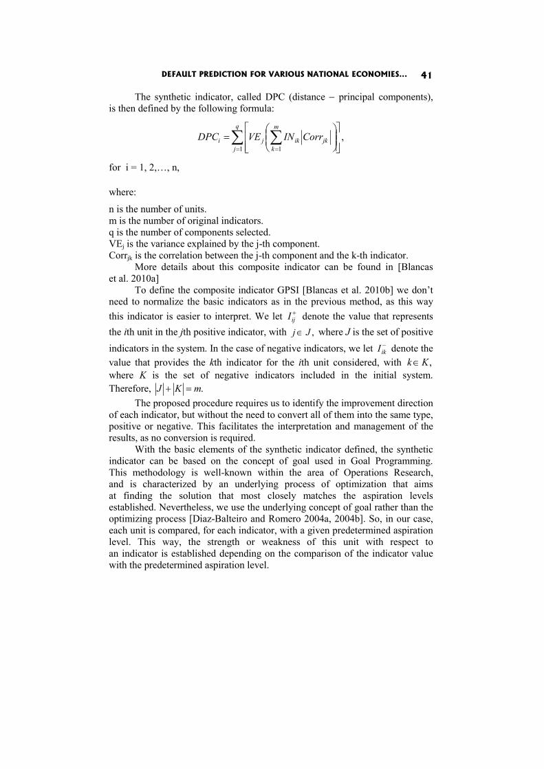
The synthetic indicator, called DPC (distance − principal components), is then defined by the following formula:
,1 1
∑ ∑= = ⎥
⎥⎦
⎤
⎢⎢⎣
⎡⎟⎟⎠
⎞⎜⎜⎝
⎛=
q
j
m
kjkikji CorrINVEDPC
for i = 1, 2,…, n, where:
n is the number of units. m is the number of original indicators. q is the number of components selected. VEj is the variance explained by the j-th component. Corrjk is the correlation between the j-th component and the k-th indicator.
More details about this composite indicator can be found in [Blancas et al. 2010a]
To define the composite indicator GPSI [Blancas et al. 2010b] we don’t need to normalize the basic indicators as in the previous method, as this way this indicator is easier to interpret. We let +
ijI denote the value that represents the ith unit in the jth positive indicator, with ,Jj ∈ where J is the set of positive indicators in the system. In the case of negative indicators, we let −
ikI denote the value that provides the kth indicator for the ith unit considered, with ,Kk ∈ where K is the set of negative indicators included in the initial system. Therefore, .mKJ =+
The proposed procedure requires us to identify the improvement direction of each indicator, but without the need to convert all of them into the same type, positive or negative. This facilitates the interpretation and management of the results, as no conversion is required.
With the basic elements of the synthetic indicator defined, the synthetic indicator can be based on the concept of goal used in Goal Programming. This methodology is well-known within the area of Operations Research, and is characterized by an underlying process of optimization that aims at finding the solution that most closely matches the aspiration levels established. Nevertheless, we use the underlying concept of goal rather than the optimizing process [Diaz-Balteiro and Romero 2004a, 2004b]. So, in our case, each unit is compared, for each indicator, with a given predetermined aspiration level. This way, the strength or weakness of this unit with respect to an indicator is established depending on the comparison of the indicator value with the predetermined aspiration level.
Rafael Caballero, Francisca García Lopera, José Enrique Padilla García, Fátima Pérez 42
In particular, we must set weights, wj, to state the relative importance of each indicator. Finally, the proposed methodology has to define an aspiration level for each indicator. +
ju will be used to refer to aspiration levels of the
positive indicators and −ku for negative indicators.
The interpretation of the aspiration level differs depending on the indicator type. In the case of positive indicators, the value establishes the minimum level at which a unit is considered to indicate a good situation regarding the aspect evaluated by the indicator. When the indicator is negative, the aspiration level reflects the maximum level that indicates a favourable situation regarding the aspect analysed.
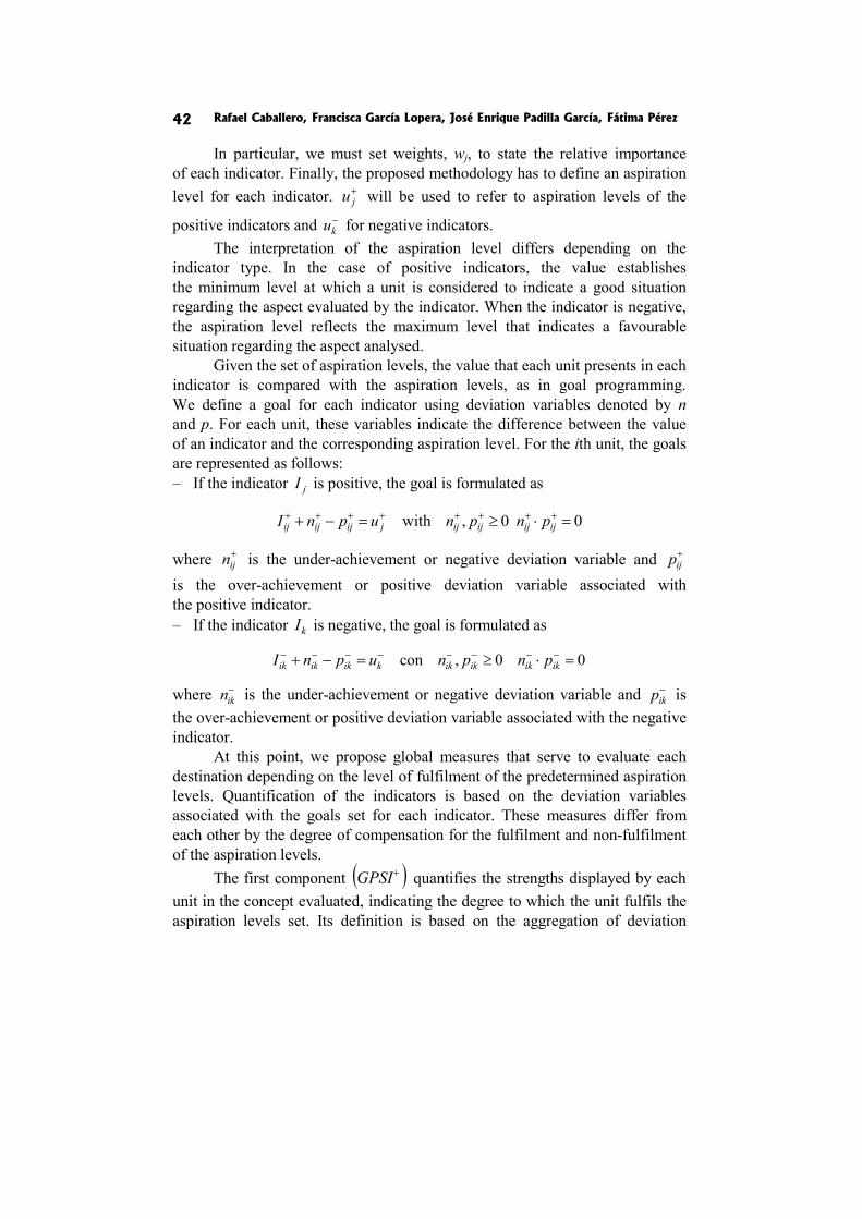
Given the set of aspiration levels, the value that each unit presents in each indicator is compared with the aspiration levels, as in goal programming. We define a goal for each indicator using deviation variables denoted by n and p. For each unit, these variables indicate the difference between the value of an indicator and the corresponding aspiration level. For the ith unit, the goals are represented as follows: – If the indicator jI is positive, the goal is formulated as
00,with =⋅≥=−+ ++++++++ijijijijjijijij pnpnupnI
where +ijn is the under-achievement or negative deviation variable and +
ijp is the over-achievement or positive deviation variable associated with the positive indicator. – If the indicator kI is negative, the goal is formulated as
00,con =⋅≥=−+ −−−−−−−−ikikikikkikikik pnpnupnI
where −ikn is the under-achievement or negative deviation variable and −
ikp is the over-achievement or positive deviation variable associated with the negative indicator.
At this point, we propose global measures that serve to evaluate each destination depending on the level of fulfilment of the predetermined aspiration levels. Quantification of the indicators is based on the deviation variables associated with the goals set for each indicator. These measures differ from each other by the degree of compensation for the fulfilment and non-fulfilment of the aspiration levels.
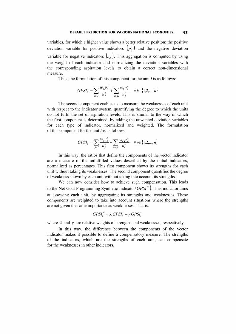
The first component ( )+GPSI quantifies the strengths displayed by each unit in the concept evaluated, indicating the degree to which the unit fulfils the aspiration levels set. Its definition is based on the aggregation of deviation
DEFAULT PREDICTION FOR VARIOUS NATIONAL ECONOMIES... 43
variables, for which a higher value shows a better relative position: the positive deviation variable for positive indicators ( )+
ijp and the negative deviation
variable for negative indicators ( )−ikn . This aggregation is computed by using
the weight of each indicator and normalizing the deviation variables with the corresponding aspiration levels to obtain a correct non-dimensional measure.
Thus, the formulation of this component for the unit i is as follows:
{ }∑ ∑∈ ∈
−
−
+
++ ∈∀+=
Jj Kk j
ikk
j
ijji ni
unw
upw
GPSI ,...,2,1
The second component enables us to measure the weaknesses of each unit with respect to the indicator system, quantifying the degree to which the units do not fulfil the set of aspiration levels. This is similar to the way in which the first component is determined, by adding the unwanted deviation variables for each type of indicator, normalized and weighted. The formulation of this component for the unit i is as follows:
{ }niu
pwu
nwGPSI
Kk k
ikk
Jj j
ijji ,...,2,1∈∀+= ∑∑
∈−
−
∈+
+−
In this way, the ratios that define the components of the vector indicator are a measure of the unfulfilled values described by the initial indicators, normalized as percentages. This first component shows its strengths for each unit without taking its weaknesses. The second component quantifies the degree of weakness shown by each unit without taking into account its strengths.
We can now consider how to achieve such compensation. This leads to the Net Goal Programming Synthetic Indicator ( )NGPSI . This indicator aims at assessing each unit, by aggregating its strengths and weaknesses. These components are weighted to take into account situations where the strengths are not given the same importance as weaknesses. That is:
−+ −= iiNi GPSIGPSIGPSI γλ
where λ and γ are relative weights of strengths and weaknesses, respectively. In this way, the difference between the components of the vector
indicator makes it possible to define a compensatory measure. The strengths of the indicators, which are the strengths of each unit, can compensate for the weaknesses in other indicators.
Rafael Caballero, Francisca García Lopera, José Enrique Padilla García, Fátima Pérez 44
2. Economic Data
In this section we are going to present the countries chosen for this paper and the indicators used. The first step is to define the theoretical framework. Eurostat [2010] has been our main source for data collection but we have also used some data from 'Global Finance 2010' database. However, we have taken into account some limitations of the theoretical framework, especially in the collecting data stage. That is why we have selected only those indicators which provide rigorous information about the variables to study. Even though Eurostat provides a lot of information about these variables, we have been interested only in those that provide relevant, complete and objective information.
According to what we have explained above, we are going to present the variables selected:
1. Debt-to-Gross Domestic Product (GDP) Ratio: this is one of the indicators of the health of an economy [Cecheti and Zampolli 2010]. It is the amount of federal debt of a country as a percentage of its Gross Domestic Product (GDP). A low debt-to-GDP ratio indicates an economy that produces a large number of goods and services and probably profits that are high enough to pay back debts.
2. Taxes Income-to- GDP Ratio: the percentage of national income that is compulsorily transferred from private pockets to the public exchequer. It is probably the most important variable. I It can be said that the value of the Debt-to-GDP Ratio is irrelevant if the country makes enough money to pay the debt.
3. Government Bond 10 years yield (in basis points, 1/100 of 1%): There is a direct relationship between the yield and the economic uncertainty of a country. It is the interest rate countries have to pay for the bond.
4. GDP real growth rate (annual %): It shows the increase or decrease in value of all final goods and services produced within a nation in a given year, taking into account inflation.
5. Credit Default Swap (in thousands of Euro): A credit default swap (CDS) is an agreement that the seller of the CDS will compensate the buyer in the event of a loan default. The buyer of the CDS makes a series of payments (the CDS “fee” or “spread”) to the seller and, in exchange, receives a payoff if the loan defaults. This might be the most difficult concept to understand.
DEFAULT PREDICTION FOR VARIOUS NATIONAL ECONOMIES... 45
This number means how much money an investor has to pay to insure 10 Million Euro Bonds. However, it is not as simple as it seems because bounds can be object of speculation in the financial markets.
6. Unemployment rate: This is an indicator of the economic activity. Moreover, less unemployment means less public expenditure and more public income so this is very important variable that affects the economy in a double sense.
7. Deficit-to-GDP Ratio: Nowadays it is a priority for all the countries to reduce the public deficit. This is also a way to reduce the public debt1.
Next step in our work is to identify the positive or negative sign for each indicator. In this sense, the sense of this paper is to analyze the bankruptcy risk for an economy so that the indicator is considered positive when higher values cause a favorable effect on the 'health' of an economy. By contrast, the indicator will be considered negative when higher values of the indicator entail harmful consequences for an economy. You can find a summary of the nature of the indicators in Table 1.
Table 1
Sign of the indicators
Indicator Description Sign 1 Debt-to-Gross Domestic Product (GDP) Ratio Negative 2 Taxes Income-to- GDP Ratio Positive 3 Bond 10 years yield (in basis points, 1/100 of 1%) Negative 4 GDP real growth rate (annual %). Positive 5 Credit Default Swap (in thousands of Euro) Negative 6 Unemployment rate Negative 7 Deficit-to-GDP Ratio Negative We have collected data for four different periods (Bloomberg, CMA
database, Markit Index, Trading Economics, 2010): first semester 2009, second semester 2009, first semester 2010 and second semester 2010 in order to show the situation in each period.
Table 2 shows all the information related to second semester 2010. Similarly, the same data have been collected for the other periods.
1 This information comes from Eurostat database, Global Finance Database and Bloomberg database.
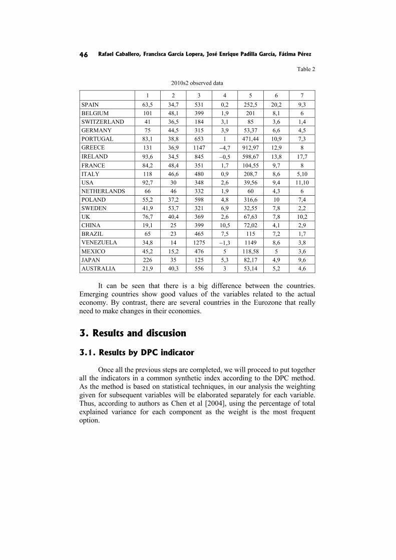
Rafael Caballero, Francisca García Lopera, José Enrique Padilla García, Fátima Pérez 46
Table 2
2010s2 observed data
1 2 3 4 5 6 7 SPAIN 63,5 34,7 531 0,2 252,5 20,2 9,3 BELGIUM 101 48,1 399 1,9 201 8,1 6 SWITZERLAND 41 36,5 184 3,1 85 3,6 1,4 GERMANY 75 44,5 315 3,9 53,37 6,6 4,5 PORTUGAL 83,1 38,8 653 1 471,44 10,9 7,3 GREECE 131 36,9 1147 −4,7 912,97 12,9 8 IRELAND 93,6 34,5 845 −0,5 598,67 13,8 17,7 FRANCE 84,2 48,4 351 1,7 104,55 9,7 8 ITALY 118 46,6 480 0,9 208,7 8,6 5,10 USA 92,7 30 348 2,6 39,56 9,4 11,10 NETHERLANDS 66 46 332 1,9 60 4,3 6 POLAND 55,2 37,2 598 4,8 316,6 10 7,4 SWEDEN 41,9 53,7 321 6,9 32,55 7,8 2,2 UK 76,7 40,4 369 2,6 67,63 7,8 10,2 CHINA 19,1 25 399 10,5 72,02 4,1 2,9 BRAZIL 65 23 465 7,5 115 7,2 1,7 VENEZUELA 34,8 14 1275 −1,3 1149 8,6 3,8 MEXICO 45,2 15,2 476 5 118,58 5 3,6 JAPAN 226 35 125 5,3 82,17 4,9 9,6 AUSTRALIA 21,9 40,3 556 3 53,14 5,2 4,6
It can be seen that there is a big difference between the countries.
Emerging countries show good values of the variables related to the actual economy. By contrast, there are several countries in the Eurozone that really need to make changes in their economies.
3. Results and discusion
3.1. Results by DPC indicator
Once all the previous steps are completed, we will proceed to put together all the indicators in a common synthetic index according to the DPC method. As the method is based on statistical techniques, in our analysis the weighting given for subsequent variables will be elaborated separately for each variable. Thus, according to authors as Chen et al [2004], using the percentage of total explained variance for each component as the weight is the most frequent option.
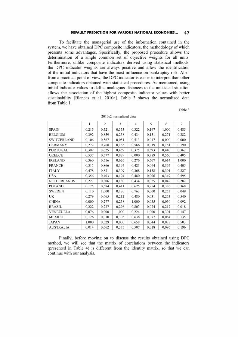
DEFAULT PREDICTION FOR VARIOUS NATIONAL ECONOMIES... 47
To facilitate the managerial use of the information contained in the system, we have obtained DPC composite indicators, the methodology of which presents some advantages. Specifically, the proposed procedure allows the determination of a single common set of objective weights for all units. Furthermore, unlike composite indicators derived using statistical methods, the DPC indicator weights are always positive and allow the identification of the initial indicators that have the most influence on bankruptcy risk. Also, from a practical point of view, the DPC indicator is easier to interpret than other composite indicators obtained with statistical procedures. As mentioned, using initial indicator values to define analogous distances to the anti-ideal situation allows the association of the highest composite indicator values with better sustainability [Blancas et al. 2010a]. Table 3 shows the normalized data from Table 1.
Table 3
2010s2 normalized data
1 2 3 4 5 6 7 SPAIN 0,215 0,521 0,353 0,322 0,197 1,000 0,485 BELGIUM 0,392 0,859 0,238 0,434 0,151 0,271 0,282 SWITZERLAND 0,106 0,567 0,051 0,513 0,047 0,000 0,000 GERMANY 0,272 0,768 0,165 0,566 0,019 0,181 0,190 PORTUGAL 0,309 0,625 0,459 0,375 0,393 0,440 0,362 GREECE 0,537 0,577 0,889 0,000 0,789 0,560 0,405 IRELAND 0,360 0,516 0,626 0,276 0,507 0,614 1,000 FRANCE 0,315 0,866 0,197 0,421 0,064 0,367 0,405 ITALY 0,478 0,821 0,309 0,368 0,158 0,301 0,227 USA 0,356 0,403 0,194 0,480 0,006 0,349 0,595 NETHERLANDS 0,227 0,806 0,180 0,434 0,025 0,042 0,282 POLAND 0,175 0,584 0,411 0,625 0,254 0,386 0,368 SWEDEN 0,110 1,000 0,170 0,763 0,000 0,253 0,049 UK 0,279 0,665 0,212 0,480 0,031 0,253 0,540 CHINA 0,000 0,277 0,238 1,000 0,035 0,030 0,092 BRAZIL 0,222 0,227 0,296 0,803 0,074 0,217 0,018 VENEZUELA 0,076 0,000 1,000 0,224 1,000 0,301 0,147 MEXICO 0,126 0,030 0,305 0,638 0,077 0,084 0,135 JAPAN 1,000 0,529 0,000 0,658 0,044 0,078 0,503 AUSTRALIA 0,014 0,662 0,375 0,507 0,018 0,096 0,196
Finally, before moving on to discuss the results obtained using DPC
method, we will see that the matrix of correlations between the indicators (presented in Table 4) is different from the identity matrix, so that we can continue with our analysis.
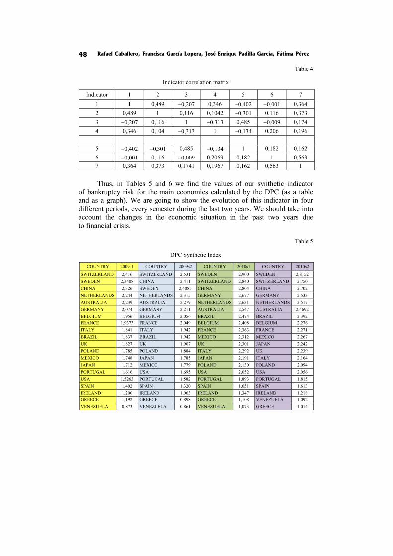
Rafael Caballero, Francisca García Lopera, José Enrique Padilla García, Fátima Pérez 48
Table 4
Indicator correlation matrix
Indicator 1 2 3 4 5 6 7 1 1 0,489 −0,207 0,346 −0,402 −0,001 0,364 2 0,489 1 0,116 0,1042 −0,301 0,116 0,373 3 −0,207 0,116 1 −0,313 0,485 −0,009 0,174 4 0,346 0,104 −0,313 1 −0,134 0,206 0,196
5 −0,402 −0,301 0,485 −0,134 1 0,182 0,162 6 −0,001 0,116 −0,009 0,2069 0,182 1 0,563 7 0,364 0,373 0,1741 0,1967 0,162 0,563 1 Thus, in Tables 5 and 6 we find the values of our synthetic indicator
of bankruptcy risk for the main economies calculated by the DPC (as a table and as a graph). We are going to show the evolution of this indicator in four different periods, every semester during the last two years. We should take into account the changes in the economic situation in the past two years due to financial crisis.
Table 5
DPC Synthetic Index
COUNTRY 2009s1 COUNTRY 2009s2 COUNTRY 2010s1 COUNTRY 2010s2
SWITZERLAND 2,416 SWITZERLAND 2,531 SWEDEN 2,900 SWEDEN 2,8152 SWEDEN 2,3408 CHINA 2,411 SWITZERLAND 2,840 SWITZERLAND 2,750 CHINA 2,326 SWEDEN 2,4085 CHINA 2,804 CHINA 2,702 NETHERLANDS 2,244 NETHERLANDS 2,315 GERMANY 2,677 GERMANY 2,533 AUSTRALIA 2,239 AUSTRALIA 2,279 NETHERLANDS 2,631 NETHERLANDS 2,517 GERMANY 2,074 GERMANY 2,211 AUSTRALIA 2,547 AUSTRALIA 2,4692 BELGIUM 1,956 BELGIUM 2,056 BRAZIL 2,474 BRAZIL 2,392 FRANCE 1,9373 FRANCE 2,049 BELGIUM 2,408 BELGIUM 2,276 ITALY 1,841 ITALY 1,942 FRANCE 2,363 FRANCE 2,271 BRAZIL 1,837 BRAZIL 1,942 MEXICO 2,312 MEXICO 2,267 UK 1,827 UK 1,907 UK 2,301 JAPAN 2,242 POLAND 1,785 POLAND 1,884 ITALY 2,292 UK 2,239 MEXICO 1,748 JAPAN 1,785 JAPAN 2,191 ITALY 2,164 JAPAN 1,712 MEXICO 1,779 POLAND 2,130 POLAND 2,094 PORTUGAL 1,616 USA 1,695 USA 2,052 USA 2,056 USA 1,5263 PORTUGAL 1,582 PORTUGAL 1,893 PORTUGAL 1,815 SPAIN 1,402 SPAIN 1,320 SPAIN 1,651 SPAIN 1,613 IRELAND 1,200 IRELAND 1,063 IRELAND 1,347 IRELAND 1,218 GREECE 1,192 GREECE 0,898 GREECE 1,108 VENEZUELA 1,092 VENEZUELA 0,873 VENEZUELA 0,861 VENEZUELA 1,073 GREECE 1,014
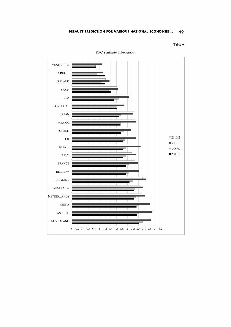
DEFAULT PREDICTION FOR VARIOUS NATIONAL ECONOMIES... 49
Table 6
DPC Synthetic Index graph
0 0,2 0,4 0,6 0,8 1 1,2 1,4 1,6 1,8 2 2,2 2,4 2,6 2,8 3 3,2
SWITZERLAND
SWEDEN
CHINA
NETHERLANDS
AUSTRALIA
GERMANY
BELGIUM
FRANCE
ITALY
BRAZIL
UK
POLAND
MEXICO
JAPAN
PORTUGAL
USA
SPAIN
IRELAND
GREECE
VENEZUELA
2010s2
2010s1
2009s2
2009s1

Rafael Caballero, Francisca García Lopera, José Enrique Padilla García, Fátima Pérez 50
From this information, we can observe two groups standing out: those situated at the top of the table and those situated at the bottom. They are always the same. The case of Venezuela is eye-catching. We are tired of hearing from the news that Mediterranean countries are likely to suffer a default. However, even if this paper confirms that fact, Venezuela presents a higher risk than any other country on the list. This is because of the CDS price and the 10-years- -bond-yield. Economic stability depends on both political situation and eco-nomic situation. In Venezuela, the political situation penalizes the economy a lot. People will not buy Venezuelan Debt if they are not sure that they will get a return. Who knows how much political and economic situation in Venezuela can change in the next ten years?
As we could anticipate, it is confirmed that countries such as China, Switzerland, Sweden or even Germany have a strong economy. The case of Japan is very interesting. Japanese Public Debt is more than 200% of GDP. However, they do not have to pay too much interest. At the same time, Japan is starting to grow after almost twenty years of economic stagnation. The situation is not as worrying as it was a couple of years ago. Anyway, the recent earthquake and tsunami will have terrible consequences also for the economy.
Lastly, we want to focus on the USA case as well. USA is penalized by a high public debt, high public deficit and taxes incomes below average. By devaluating the dollar, they want people to buy US production but this solution is recommendable in the very short term only, in the long term it could cause inflation and other harmful consequences to the economy. To summarize, there are three different groups of countries: Those whose economies enjoy perfect health, those that really have to apply contracting monetary (if possible) and fiscal policies and, finally, countries in the middle with very different characteristics (the cases of United Kingdom, Brazil, Japan and so on).
3.2. Results by GPSI indicator
We are presenting a new methodology which offers several advantages over existing ones. In particular, it is designed to be practical and to facilitate obtaining easy-to-interpret synthetic indicators. Inspired by goal programming, this method allows us to obtain several synthetic indicators based on infor-mation provided by the goals corresponding to each indicator.
DEFAULT PREDICTION FOR VARIOUS NATIONAL ECONOMIES... 51
The difference between the synthetic measures proposed is reflected by the degree of compensation of fulfillment and non fulfillment of the aspiration levels. In any case, these measures assess each unit, accounting for their strengths and weaknesses, which can be analyzed together or separately. Interpreting the values of the synthetic indicator is easy, because the results are expressed in terms of proximity to the reference situation defining the goals.
The methodology we develop is not a technique based on statistics for the process of weighting the different indicators that will form our composite index of bankruptcy risk. For its development, we will use some previously established steps. In this case it is not necessary to normalize the data but we will use again the positive or negative effect of the indicator (presented in Table 2). However, it will be necessary to add the concept of neutrality of the indicator (when it reaches a specific value, the desired reference level). We have defined what we consider to be the reference level for every indicator. Nowadays, it makes no sense to fix the average point as the desired level because given the delicate situation of the world economy the average point will be a non-desirable point for the governments. The result is a synthetic indicator vector (called GPSIv), composed of a two components vector (GPSI+, GPSI-). According to Blancas et al. [2010a, p. 10] “the first component of vector synthetic indicator shows the strengths for each unit while ignoring their weaknesses. The second component quantifies the degree of weakness shown by each unit while ignoring their strengths. Neutral indicators are represented by their weaknesses only, because the deviation of variables indicates weakness only”. Thus, given the synthetic indicator vector of goal programming GPSIv, we note that the comparison is very complicated. In this way, to make the comparison easy-to-interpret we are going to use the Synthetic Index based on Restrictive Goal Programming (GPSIR) and the Synthetic Index based on Net Goal Programming (GPSIN). The GPSIR is based on the idea of distinction of the units that fulfill the levels of reference and, as opposed to the GPSIv, it does not compensate strengths and weaknesses. As for the GPIN, it combines strengths and weaknesses, each with a different weighting. The results obtained by using this method can be seen in the next tables.

Rafael Caballero, Francisca García Lopera, José Enrique Padilla García, Fátima Pérez 52
Table 7
Net GPSI Synthetic Indicator for 1st and 2nd semester 2009
COUNTRY 2009s1 GPSI + GPSI − NET GPSI COUNTRY
2009s2 GPSI + GPSI − NET GPSI
CHINA 4,12 0,46 3,67 CHINA 3,9 0,47 3,43 AUSTRALIA 2,36 1,25 1,11 AUSTRALIA 1,91 1,21 0,7 SWITZERLAND 2,45 2,56 −0,11 SWITZERLAND 2,66 2,3 0,36 SWEDEN 2,87 3,56 −0,69 SWEDEN 2,64 3 −0,36 NETHERLANDS 1,8 3,76 −1,96 NETHERLANDS 1,56 3,25 −1,69 BRAZIL 1 3,71 −2,71 BRAZIL 0,84 3,78 −2,94 GERMANY 1,81 4,59 −2,78 GERMANY 1,7 3,94 −2,24 FRANCE 0,88 4,27 −3,38 FRANCE 0,87 4,41 −3,54 USA 0,76 4,4 −3,64 USA 0,88 4,65 −3,77 UK 0,8 4,44 −3,64 UK 0,71 4,56 −3,86 MEXICO 1,12 5,5 −4,39 MEXICO 0,78 5,6 −4,82 BELGIUM 1,27 7,37 −6,1 BELGIUM 0,95 6,92 −5,97 POLAND 0,63 7,06 −6,43 POLAND 0,45 6,98 −6,53 SPAIN 0,01 7,52 −7,5 ITALY 0,93 8,61 −7,68 JAPAN 1,42 9,06 −7,64 JAPAN 1,43 9,72 −8,29 ITALY 1,17 8,88 −7,71 SPAIN 0,03 10,25 −10,22 PORTUGAL 0,49 12,29 −11,8 PORTUGAL 0,39 12,39 −12,01 IRELAND 0,28 16,89 −16,61 IRELAND 0,08 17,07 −16,99 GREECE 0,41 22,57 −22,16 VENEZUELA 0,4 26,16 −25,75 VENEZUELA 0,74 28,01 −27,27 GREECE 0,35 26,18 −25,83

DEFAULT PREDICTION FOR VARIOUS NATIONAL ECONOMIES... 53
Table 8
Net GPSI Synthetic Indicator for 1st and 2nd semester 2010
COUNTRY 2010s1 GPSI+ GPSI − NET GPSI COUNTRY
2010s2 GPSI + GPSI − NET GPSI
CHINA 6,36 0,47 5,89 CHINA 6,47 0,47 6 SWEDEN 4,39 0,13 4,26 SWEDEN 5,16 0,14 5,02 SWITZERLAND 2,99 0,58 2,41 SWITZERLAND 3,27 0,58 2,69 GERMANY 3,05 1,18 1,87 AUSTRALIA 2,29 0,49 1,8 AUSTRALIA 2,18 0,49 1,69 BRAZIL 4,18 2,5 1,67 BRAZIL 4,06 2,5 1,55 GERMANY 2,55 1,21 1,34 NETHERLANDS 1,61 0,84 0,76 MEXICO 2,67 2,21 0,46 MEXICO 2,34 2,2 0,13 NETHERLANDS 1,31 0,97 0,34 UK 1,1 1,87 −0,77 UK 0,98 1,99 −1,01 USA 1,21 2,65 −1,44 USA 1,19 2,65 −1,45 FRANCE 0,98 2,52 −1,53 FRANCE 0,79 2,81 −2,02 BELGIUM 1,48 4,83 −3,35 JAPAN 3,28 6,97 −3,69 JAPAN 2,25 6,87 −4,62 BELGIUM 0,82 4,96 −4,13 ITALY 0,89 5,84 −4,95 POLAND 1,85 6,66 −4,81 POLAND 1,22 6,53 −5,31 ITALY 0,88 6,48 −5,6 SPAIN 0,03 7,02 −6,99 SPAIN 0,03 7,3 −7,26 PORTUGAL 0,27 10,89 −10,63 PORTUGAL 0,28 11,47 −11,19 IRELAND 0,03 16,67 −16,64 IRELAND 0,03 17,63 −17,61 GREECE 0,12 26 −25,88 GREECE 0,1 26,95 −26,85 VENEZUELA 0,45 27,96 −27,51 VENEZUELA 0,79 27,68 −26,89

Rafael Caballero, Franc54
N
We can clearly st
the countries. That could Once again, we have the middle of the table. VeneAs we can see, it has muccountries at the bottom bstriking. Nobody is surpris that they can keep impstrengths but the weakne
-30 -25
CHINA
AUSTRALIA
SWITZERLAND
SWEDEN
NETHERLANDS
BRAZIL
GERMANY
FRANCE
USA
UK
MEXICO
BELGIUM
POLAND
SPAIN
JAPAN
ITALY
PORTUGAL
IRELAND
GREECE
VENEZUELA
cisca García Lopera, José Enrique Padilla García, Fátima Pé
Tab
Net GPSI Synthetic Indicator Graph
ate that the situation has improved for almostmean that we are getting over the economic crsame economies at the top, at the bottom and inezuela is again penalized by the highest CDS prch more strengths (0,79 in 2010s2) than the rest ofbut also more weaknesses. The case of China is rised to see China at the top of this table. The pproving its situation because its problems are not esses. Once again, Switzerland is situated in a v
-20 -15 -10 -5 0 5 10
2010
2010
2009
2009
érez
ble 9
t all risis. n the rice. f the also
point the very
0s2
0s1
9s2
9s1
DEFAULT PREDICTION FOR VARIOUS NATIONAL ECONOMIES... 55
comfortable situation. That is explained by the combination of high public incomes, low deficit, low unemployment and low debt. The tables show that Portugal's situation is very dangerous; it is just behind some countries that have already been rescued. It might be the next if it does not carry out restrictive policies and economic cuts.
3.3. Discusion of results
Once the results have been analyzed using both methods, one based on statistical techniques (Distance-Principal Components method), and one based on non-statistical techniques (Goal Programming Synthetic Indicator and its variants) in this section we will discuss the advantages and disadvantages of each by trying to compare the results, in order to find common patterns of behavior among different countries.
Some advantages of the DPC method come from the fact that it re-presents most of the information provided by the system with a limited number of variables, uncorrelated [Blancas et al. 2010b]. Moreover, comparative analysis is very simple and intuitive. Furthermore, as we said above, the method itself is responsible for providing the weights, without any interference by expert groups (which always brings subjectivity to the analysis).
As regards the GPSI method, and following Blancas et al. [2010a], it has a number of advantages over statistical methods. The first one is that it does not require prior normalization of the data. Moreover, this technique admits a number of indicators lower than the number of observations. Furthermore, there is no a lack of information, since all indicators from the initial system are used to build the synthetic indicator. There are a number of drawbacks, since the analyst is obliged to make decisions, both in the setting of weights and in the aspiration levels for each indicator. Below, we try to summarize and compare the results we have obtained by using each method. We will only focus on the 2010 second semester rankings because they are the most recent information we can analyze.
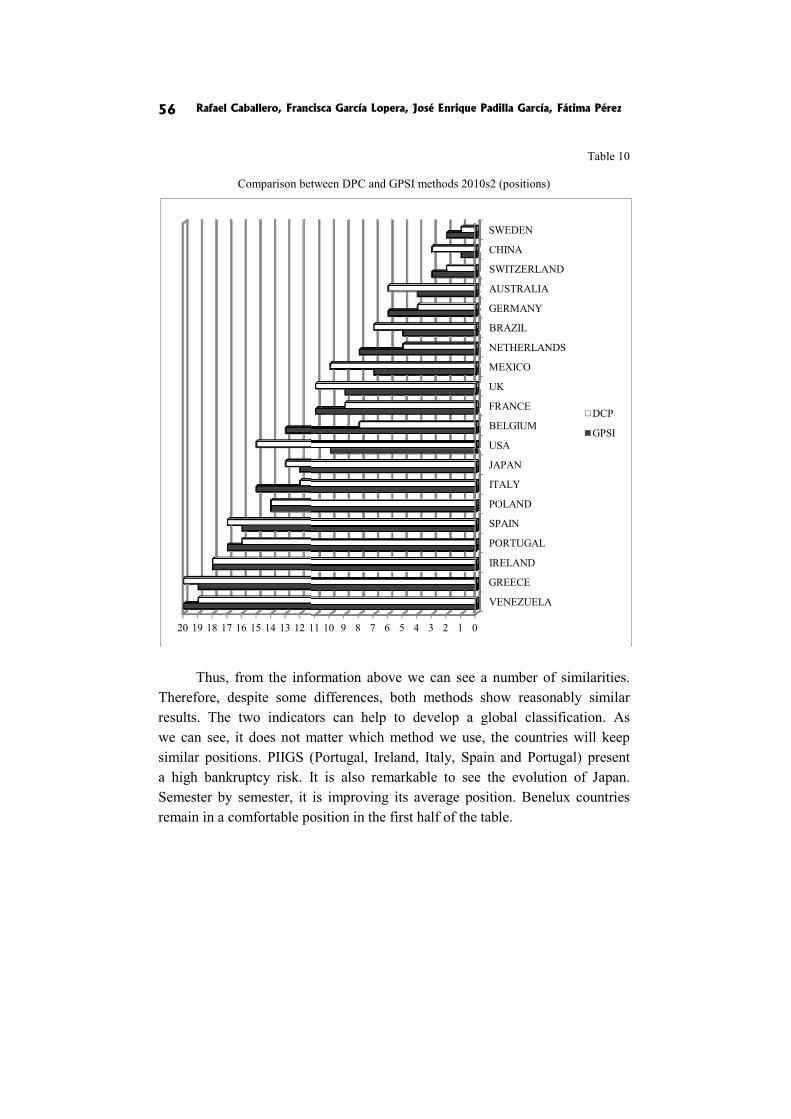
Rafael Caballero, Franc56
Comparison bet
Thus, from the info
Therefore, despite some results. The two indicatowe can see, it does not msimilar positions. PIIGS (a high bankruptcy risk. ISemester by semester, it remain in a comfortable po
1121314151617181920
cisca García Lopera, José Enrique Padilla García, Fátima Pé
Tabl
tween DPC and GPSI methods 2010s2 (positions)
ormation above we can see a number of similaritdifferences, both methods show reasonably sim
ors can help to develop a global classification. matter which method we use, the countries will k(Portugal, Ireland, Italy, Spain and Portugal) preIt is also remarkable to see the evolution of Japis improving its average position. Benelux countosition in the first half of the table.
01234567891011
SWEDEN
CHINA
SWITZERLAND
AUSTRALIA
GERMANY
BRAZIL
NETHERLANDS
MEXICO
UK
FRANCE
BELGIUM
USA
JAPAN
ITALY
POLAND
SPAIN
PORTUGAL
IRELAND
GREECE
VENEZUELA
DC
GP
érez
le 10
ties. milar
As keep sent pan. tries
CP
SI
DEFAULT PREDICTION FOR VARIOUS NATIONAL ECONOMIES... 57
As a conclusion from these data, it seems clear which countries are likely to default. 'Piigs' and Venezuela are in a very dangerous situation. However, the causes of this harmful situation depend on the countries. For instance, Venezuela is affected by high prices for the variables negotiated in the financial markets due to its political system, Spain is penalized by the highest unemployment in the UE27 and Greece and Ireland have enormous problems with their bank system and their public debt. The case of Portugal is also complicated. It combines a political problem and a difficult economic situation. As long as politicians do not carry out restrictive policies Portugal will be more vulnerable to default.
Conclusions
Throughout this paper we have analyzed the current problem of bankruptcy risk for the main economies in the world. Before the financial crisis originated in the United States in the summer 2007, it was difficult to imagine that countries such as Greece or Ireland might have to ask for external help. However, this crisis has uncovered the shortages of all economies. As we can see, some countries have been able to recover their GDP and employment rate at the same level as before the crisis. However, countries that already had a structural problem in their economies have been strongly hit by the crisis. Such are the cases of Spain and the property bubble, Ireland and the bank system crisis or Greece. Crisis has only accelerated the process of adjustment.
Thus, throughout this paper we have carried out an assessment of the situation in the EU-27 based on data from Eurostat [2010], by constructing a synthetic index of bankruptcy risk through different methods (the Distance-Principal Components, based on statistical techniques, and goal programming techniques which are not based on statistics), each of them with its pros and cons, keeping in mind that the indicator is not an end in itself but an instrument available to the researcher for better analysis of the situation. Despite the great subjectivity that underlies the construction of such indicators, we have tried to be as explicit as possible in the methodological aspects with intent to make our analysis objective and give it validity and scientific rigor.
To sum up, not only is it important to have a stable economy but it is equally important to convince people that your country has a powerful eco-nomy. Otherwise, if there is uncertainty about the economic situation, the
Rafael Caballero, Francisca García Lopera, José Enrique Padilla García, Fátima Pérez 58
financial market will punish that economy. As we have seen, economic stability depends on actual economic variables and those negotiated in the financial markets.
Acknowledgements
The authors wish to express their gratitude to the referees for their valuable and helpful comments, which have improved the quality of the paper. This research has been partially funded by the research projects of the Andalusian Regional Government.
References
Blancas F.J., Caballero R., González M., Lozano-Oyola M., Pérez F. (2010a), Goal Programming Synthetic Indicators: An Application for Sustainable Tourism in Andalusian Coastal Counties, “Ecological Economics”, No. 69.
Blancas F.J., González M., Lozano-Oyola M., Pérez F. (2010b), The Assessment of a Sustainable Tourism: Application to Spanish Coastal Destinations, “Ecolo-gical Indicators”, No. 10.
Bloomberg, www.bloomberg.com Cechetti S., Zampolli F. (2010), The Future of Public Debt: Prospects and Implications,
ISSN 1020-0959 (print) ISBN 1682-7678 (online). Chen C.J., Fu X.F., Ma X.W. (2004), Research on Sustainable Development with
Regards to the Economic System and the Energy System in Mainland China, “International Journal of Global Energy”, No. 22.
CMA database, www.cmavision.com Diaz-Balteiro L., Romero C., (2004a), In Search of a Natural Systems Sustainability
Index, “Ecol. Econ.”, No. 49. Diaz-Balteiro L., Romero C., (2004b), Sustainability of Forest Management Plans:
A Discrete Goal Programming Approach, “J. Environ. Manage.” No. 71. Eurostat (2010), Euroarea and EU27 Government Deficit at 6.3% and 6.8% of GDP
Respectively, Eurostat new release indicators. Kan Y.H. and Pedersen, C. (2011), The Impact of Margin Interest on the Evaluation
of Credit Default Swaps, Working Paper, University o Columbia Markit Index, http://indices.markit.com/default.asp Nardo M., Saisana M., Saltelli A., Tarantola, S., Hoffman, A., Giovannini, E. (2008),
Handbook on Constructing Composite Indicators: Methodology and User Guide, OECD Statistics Working Papers.
Trading economics, www.tradingeconomics.com
Cezary Dominiak
THE DISCRETE INTERACTIVE MULTIPLE GOAL PROGRAMMING UNDER RISK
Abstract
An Interactive Multiple Goal Programming (IMGP) is a popular method of multicriteria decision aiding. The discrete version of this method was proposed by Habenicht in 1984. In this paper we propose the modification of discrete version IMGP which enables us to take into consideration risk factors and it’s also adopted for group decision making.. Risky criteria are described by probability distributions. The aggre-gation of local judgments making by individual decision makers to the group decision is carried out by voting system. In this paper proposed method is presented. In the last section the proposed method is illustrated by simple numerical example.
Keywords
Multicriteria decision making, decisions under risk, group decision making.
Introduction
In the beginning of the 21st century we observe a significant volatility of the macroeconomic environment, which has a considerable impact on the business world. First of all it is a consequence of rapid technological progress, particularly in the field of information and telecommunication technologies (ICT) and the increasing economic globalization.
In consequence, the influence that these factors exert on economic and business decisions has to be taken into account in the decision-making. The issues related to decision analysis and aiding under incomplete information remain an important part of operational research, in particular of multicriteria decision aiding. Uncertainty implies that in certain situations a person does not possess the information which is quantitatively and qualitatively appropriate to describe, prescribe or predict deterministically and numerically a system, its behavior or other characteristics [Zimmerman 2000].
Cezary Dominiak 60
In the MCDA approach we can find a wide range of methods and techniques to deal with uncertainty: sensitivity analysis [e.g. Rios Insua 1990], fuzzy set approach [e.g. Klir and Fogler 1988], rough set approach [e.g. Greco, Matarazzo and Slowinski 1999], probabilistic models and expected utility [Bazerman 2002; Rosquist 2001], pairwise comparisons based on stochastic dominance [e.g. Martel and Zaras 1995; Nowak 2008]. Rrisk measures as surrogate criteria are also applied [e.g. Millet and Wedley 2002; Jia and Dyer 1996].
In business organizations we observe that very often a Decision Maker (DM) is not a single person but a group of people responsible for making a decision. Thus the modeling of group preferences becomes an important part of the decision making process. The problems of group decision making is discussed, for example, by Ramanathan and Ganesh [1994], Van Den Honert [2001], Herrera, Martınez and Sanchez [2005].
In this paper we propose an interactive procedure which is a modification of the discrete version of Interactive Multiple Goal Programming (IMGP) which enables decision aiding under risk by a group of decision makers. The first section of this paper shortly describes the IMGP algorithm and its main advantages. The second section presents the proposed decision aiding method. A simple numerical example is presented in the last part of this paper.
1. The Interactive Multiple Goal Programming
The IMGP was proposed by Nijkamp and Spronk [1980]. According to this approach, the single criterion problems are solved first. Then, on the basis of the optimal solutions obtained the potency matrix is calculated. The potency matrix consists of the ideal solution and the current one. The DM chooses the criterion on which the current solution should be improved and describes the aspiration level for this criterion. The proper constraint is added to each single criterion problem considered and then those problems are solved again. The DM compares the obtained values in the potency matrixes and decides whether he/she accepts the new solution or not. The procedure is continued till the ideal and the current solutions become equal to each other. Some important advantages are connected with the IMGP. First of all, the DM does not have to give his preference information on an a priori basis but has to consider all kinds of choices and trade-off questions which may be relevant [see Nijkamp

THE DISCRETE INTERACTIVE MULTIPLE GOAL PROGRAMMING... 61
1980, p. 104]. Another important advantage of IMGP is its relatively simply and easy to understand idea. During an interactive procedure the DM has to answer the simple questions:
1 Is the given solution acceptable or not? 2. Which goal value needs to be improved? 3. How much should this goal value be improved at least? 4. Does he accept the consequences of the proposed improvement
of the value of the indicated goal variable? [see Nijkamp 1980, p. 250]. The discrete version of IMGP was proposed by Habenicht [1984]. In this
case instead of a multicriteria linear programming problem we consider a finite set of alternatives. Each alternative is described by a finite set of attributes. The potency matrixes are calculated on the basis of criteria values within the set of alternatives and in each iteration according to the DM’s decisions the set of alternatives is reduced.
2. The discrete IMGP under Risk
In this section we propose an interactive multicriteria decision aiding method which supports multictiteria group decision making under uncertainty for discrete decision problems. Let us assume that: m − is the number of alternatives, k − is the number of criteria, all criteria are maximized, Xi,j − is the probability distribution of the j-th criterion of the i-th alternative, pj − is the probability at which the j-th criterion is evaluated.
Moreover, let us assume that the matrix
mkijj xpX ][)( =
includes the values of the j-th evaluation criterion for the assumed probability value pj, and these values guarantee the probability that a particular variable will have a lower value of at least pj, which is defined as follows:
jjiji pxXP =≥ )( ,,
Let xideal denote the ideal solution, defined below: ],...,1;
,...,1max:,[)( , kjx
mixxpx ijjijijideal =
===
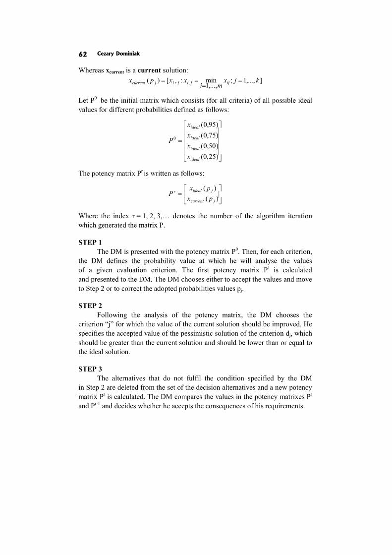
Cezary Dominiak 62
Whereas xcurrent is a current solution: ],...,1;
,...,1min:,[)( , kjx
mixxpx ijjijijcurrent =
===
Let P0 be the initial matrix which consists (for all criteria) of all possible ideal values for different probabilities defined as follows:
⎥⎥⎥⎥
⎦
⎤
⎢⎢⎢⎢
⎣
⎡
=
)25,0()50,0()75,0()95,0(
0
ideal
ideal
ideal
ideal
xxxx
P
The potency matrix Pr is written as follows:
⎥⎦
⎤⎢⎣
⎡=
)()(
jcurrent
jidealr
pxpx
P
Where the index r = 1, 2, 3,… denotes the number of the algorithm iteration which generated the matrix P.
STEP 1 The DM is presented with the potency matrix P0. Then, for each criterion,
the DM defines the probability value at which he will analyse the values of a given evaluation criterion. The first potency matrix P1 is calculated and presented to the DM. The DM chooses either to accept the values and move to Step 2 or to correct the adopted probabilities values pj.
STEP 2 Following the analysis of the potency matrix, the DM chooses the
criterion “j” for which the value of the current solution should be improved. He specifies the accepted value of the pessimistic solution of the criterion dj, which should be greater than the current solution and should be lower than or equal to the ideal solution.
STEP 3 The alternatives that do not fulfil the condition specified by the DM
in Step 2 are deleted from the set of the decision alternatives and a new potency matrix Pr is calculated. The DM compares the values in the potency matrixes Pr and Pr-1 and decides whether he accepts the consequences of his requirements.
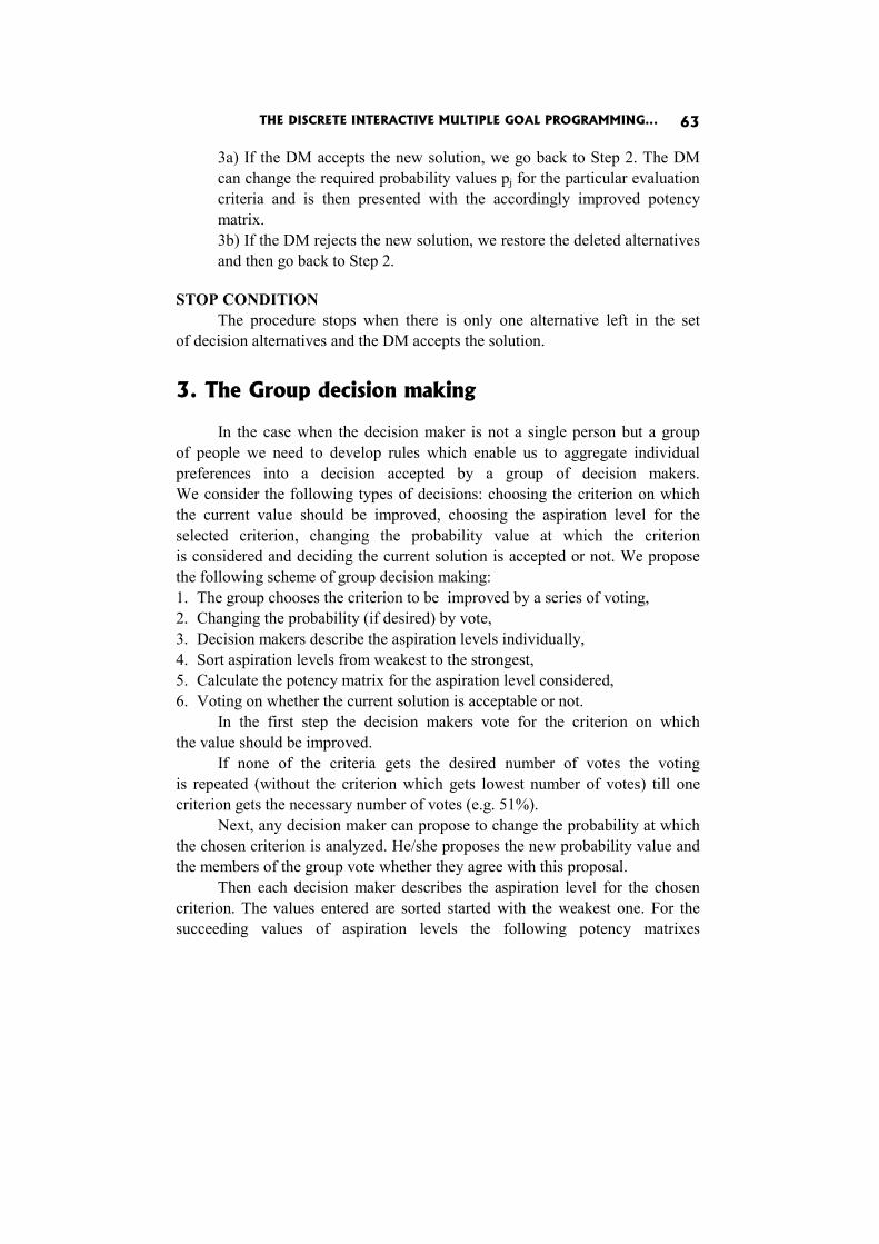
THE DISCRETE INTERACTIVE MULTIPLE GOAL PROGRAMMING... 63
3a) If the DM accepts the new solution, we go back to Step 2. The DM can change the required probability values pj for the particular evaluation criteria and is then presented with the accordingly improved potency matrix. 3b) If the DM rejects the new solution, we restore the deleted alternatives and then go back to Step 2.
STOP CONDITION The procedure stops when there is only one alternative left in the set
of decision alternatives and the DM accepts the solution.
3. The Group decision making
In the case when the decision maker is not a single person but a group of people we need to develop rules which enable us to aggregate individual preferences into a decision accepted by a group of decision makers. We consider the following types of decisions: choosing the criterion on which the current value should be improved, choosing the aspiration level for the selected criterion, changing the probability value at which the criterion is considered and deciding the current solution is accepted or not. We propose the following scheme of group decision making: 1. The group chooses the criterion to be improved by a series of voting, 2. Changing the probability (if desired) by vote, 3. Decision makers describe the aspiration levels individually, 4. Sort aspiration levels from weakest to the strongest, 5. Calculate the potency matrix for the aspiration level considered, 6. Voting on whether the current solution is acceptable or not.
In the first step the decision makers vote for the criterion on which the value should be improved.
If none of the criteria gets the desired number of votes the voting is repeated (without the criterion which gets lowest number of votes) till one criterion gets the necessary number of votes (e.g. 51%).
Next, any decision maker can propose to change the probability at which the chosen criterion is analyzed. He/she proposes the new probability value and the members of the group vote whether they agree with this proposal.
Then each decision maker describes the aspiration level for the chosen criterion. The values entered are sorted started with the weakest one. For the succeeding values of aspiration levels the following potency matrixes
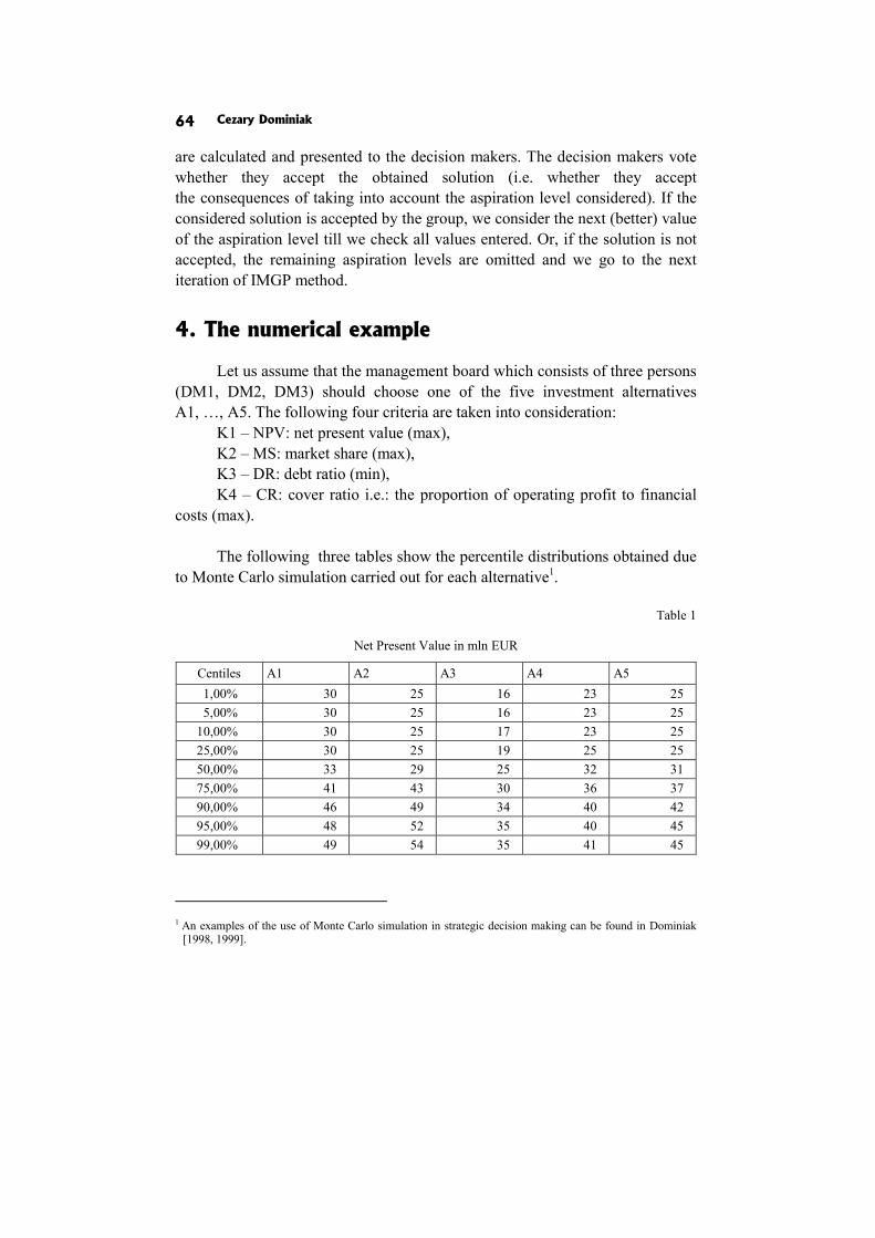
Cezary Dominiak 64
are calculated and presented to the decision makers. The decision makers vote whether they accept the obtained solution (i.e. whether they accept the consequences of taking into account the aspiration level considered). If the considered solution is accepted by the group, we consider the next (better) value of the aspiration level till we check all values entered. Or, if the solution is not accepted, the remaining aspiration levels are omitted and we go to the next iteration of IMGP method.
4. The numerical example
Let us assume that the management board which consists of three persons (DM1, DM2, DM3) should choose one of the five investment alternatives A1, …, A5. The following four criteria are taken into consideration:
K1 – NPV: net present value (max), K2 – MS: market share (max), K3 – DR: debt ratio (min), K4 – CR: cover ratio i.e.: the proportion of operating profit to financial
costs (max). The following three tables show the percentile distributions obtained due
to Monte Carlo simulation carried out for each alternative1.
Table 1
Net Present Value in mln EUR
Centiles A1 A2 A3 A4 A5 1,00% 30 25 16 23 25 5,00% 30 25 16 23 25
10,00% 30 25 17 23 25 25,00% 30 25 19 25 25 50,00% 33 29 25 32 31 75,00% 41 43 30 36 37 90,00% 46 49 34 40 42 95,00% 48 52 35 40 45 99,00% 49 54 35 41 45
1 An examples of the use of Monte Carlo simulation in strategic decision making can be found in Dominiak
[1998, 1999].
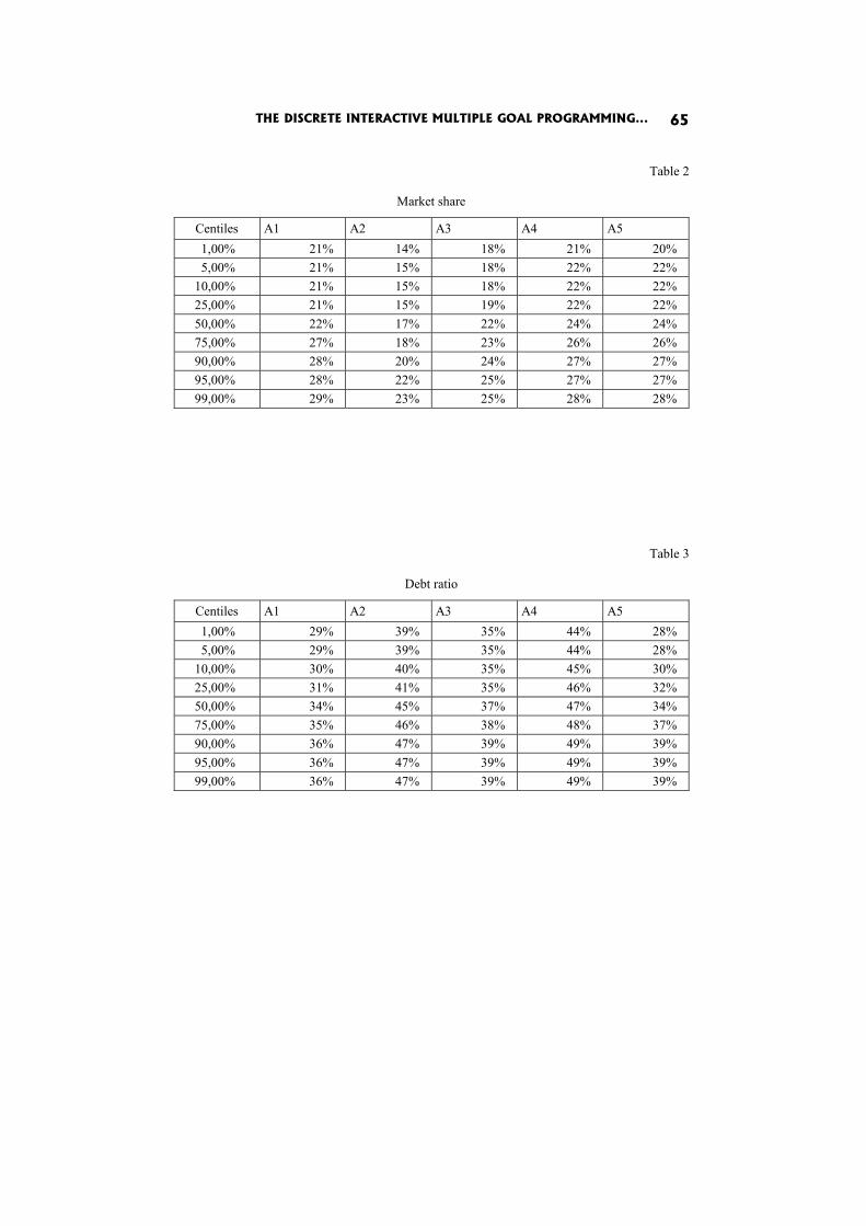
THE DISCRETE INTERACTIVE MULTIPLE GOAL PROGRAMMING... 65
Table 2
Market share
Centiles A1 A2 A3 A4 A5 1,00% 21% 14% 18% 21% 20% 5,00% 21% 15% 18% 22% 22%
10,00% 21% 15% 18% 22% 22% 25,00% 21% 15% 19% 22% 22% 50,00% 22% 17% 22% 24% 24% 75,00% 27% 18% 23% 26% 26% 90,00% 28% 20% 24% 27% 27% 95,00% 28% 22% 25% 27% 27% 99,00% 29% 23% 25% 28% 28%
Table 3
Debt ratio
Centiles A1 A2 A3 A4 A5 1,00% 29% 39% 35% 44% 28% 5,00% 29% 39% 35% 44% 28%
10,00% 30% 40% 35% 45% 30% 25,00% 31% 41% 35% 46% 32% 50,00% 34% 45% 37% 47% 34% 75,00% 35% 46% 38% 48% 37% 90,00% 36% 47% 39% 49% 39% 95,00% 36% 47% 39% 49% 39% 99,00% 36% 47% 39% 49% 39%
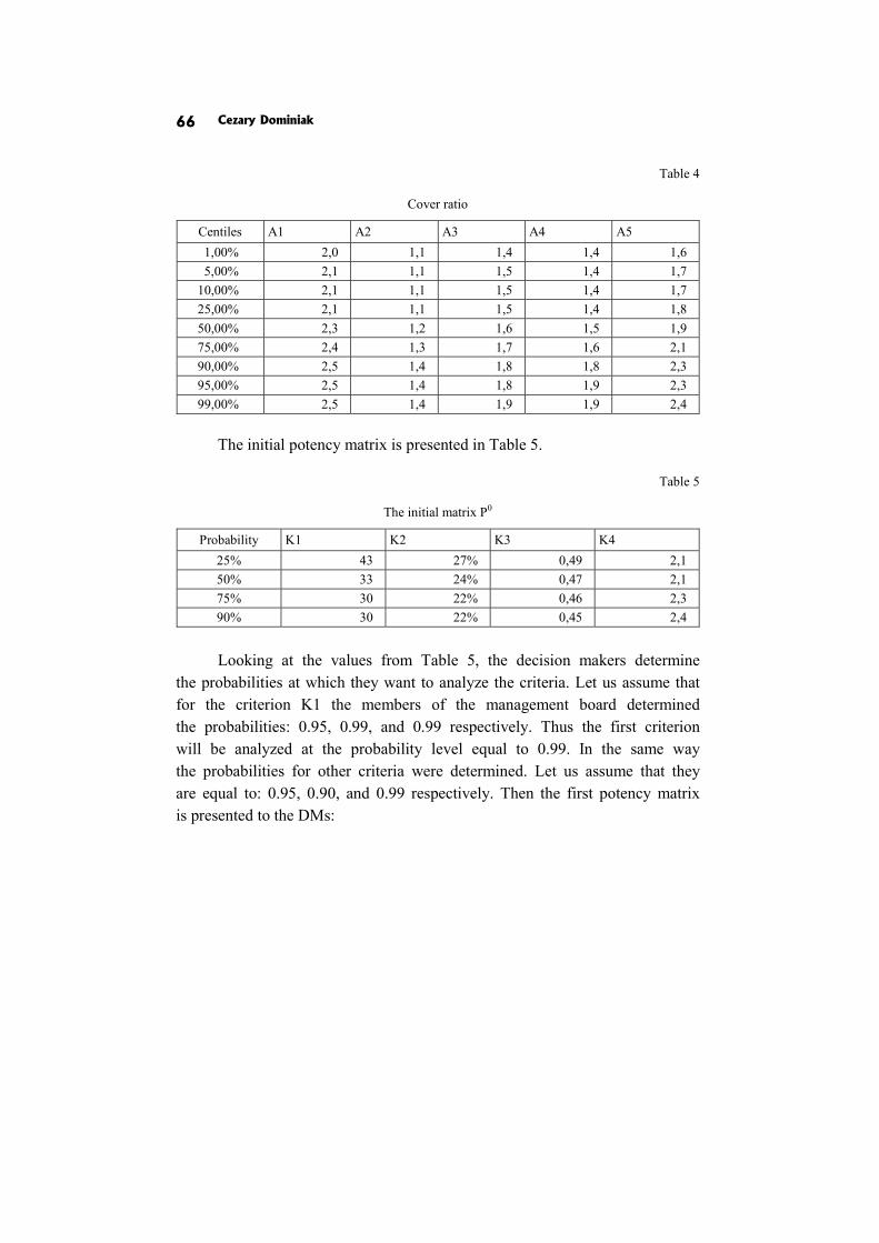
Cezary Dominiak 66
Table 4
Cover ratio
Centiles A1 A2 A3 A4 A5 1,00% 2,0 1,1 1,4 1,4 1,6 5,00% 2,1 1,1 1,5 1,4 1,7
10,00% 2,1 1,1 1,5 1,4 1,7 25,00% 2,1 1,1 1,5 1,4 1,8 50,00% 2,3 1,2 1,6 1,5 1,9 75,00% 2,4 1,3 1,7 1,6 2,1 90,00% 2,5 1,4 1,8 1,8 2,3 95,00% 2,5 1,4 1,8 1,9 2,3 99,00% 2,5 1,4 1,9 1,9 2,4
The initial potency matrix is presented in Table 5.
Table 5
The initial matrix P0
Probability K1 K2 K3 K4 25% 43 27% 0,49 2,1 50% 33 24% 0,47 2,1 75% 30 22% 0,46 2,3 90% 30 22% 0,45 2,4 Looking at the values from Table 5, the decision makers determine
the probabilities at which they want to analyze the criteria. Let us assume that for the criterion K1 the members of the management board determined the probabilities: 0.95, 0.99, and 0.99 respectively. Thus the first criterion will be analyzed at the probability level equal to 0.99. In the same way the probabilities for other criteria were determined. Let us assume that they are equal to: 0.95, 0.90, and 0.99 respectively. Then the first potency matrix is presented to the DMs:
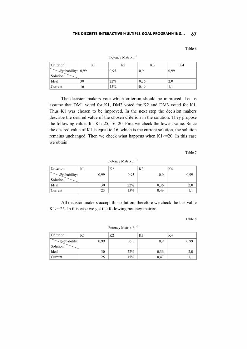
THE DISCRETE INTERACTIVE MULTIPLE GOAL PROGRAMMING... 67
Table 6
Potency Matrix P1
Criterion: K1 K2 K3 K4 Probability:
Solution: 0,99 0,95 0,9 0,99
Ideal 30 22% 0,36 2,0 Current 16 15% 0,49 1,1
The decision makers vote which criterion should be improved. Let us
assume that DM1 voted for K1, DM2 voted for K2 and DM3 voted for K1. Thus K1 was chosen to be improved. In the next step the decision makers describe the desired value of the chosen criterion in the solution. They propose the following values for K1: 25, 16, 20. First we check the lowest value. Since the desired value of K1 is equal to 16, which is the current solution, the solution remains unchanged. Then we check what happens when K1>=20. In this case we obtain:
Table 7
Potency Matrix P1-1
Criterion: K1 K2 K3 K4 Probability:
Solution: 0,99 0,95 0,9 0,99
Ideal 30 22% 0,36 2,0 Current 23 15% 0,49 1,1
All decision makers accept this solution, therefore we check the last value
K1>=25. In this case we get the following potency matrix:
Table 8
Potency Matrix P1-2
Criterion: K1 K2 K3 K4 Probability:
Solution: 0,99 0,95 0,9 0,99
Ideal 30 22% 0,36 2,0 Current 25 15% 0,47 1,1
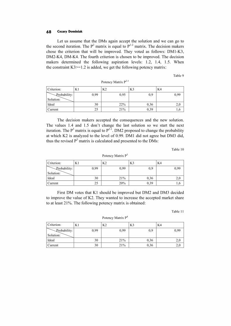
Cezary Dominiak 68
Let us assume that the DMs again accept the solution and we can go to the second iteration. The P2 matrix is equal to P1-2 matrix. The decision makers chose the criterion that will be improved. They voted as follows: DM1-K3, DM2-K4, DM-K4. The fourth criterion is chosen to be improved. The decision makers determined the following aspiration levels: 1.2, 1.4, 1.5. When the constraint K3>=1.2 is added, we get the following potency matrix:
Table 9
Potency Matrix P2-1
Criterion: K1 K2 K3 K4 Probability:
Solution: 0,99 0,95 0,9 0,99
Ideal 30 22% 0,36 2,0 Current 25 21% 0,39 1,6
The decision makers accepted the consequences and the new solution.
The values 1.4 and 1.5 don’t change the last solution so we start the next iteration. The P3 matrix is equal to P2-1. DM2 proposed to change the probability at which K2 is analyzed to the level of 0.99. DM1 did not agree but DM3 did, thus the revised P3 matrix is calculated and presented to the DMs:
Table 10
Potency Matrix P3
Criterion: K1 K2 K3 K4 Probability:
Solution: 0,99 0,99 0,9 0,99
Ideal 30 21% 0,36 2,0 Current 25 20% 0,39 1,6
First DM votes that K1 should be improved but DM2 and DM3 decided
to improve the value of K2. They wanted to increase the accepted market share to at least 21%. The following potency matrix is obtained:
Table 11
Potency Matrix P4
Criterion: K1 K2 K3 K4 Probability:
Solution: 0,99 0,99 0,9 0,99
Ideal 30 21% 0,36 2,0 Current 30 21% 0,36 2,0
THE DISCRETE INTERACTIVE MULTIPLE GOAL PROGRAMMING... 69
Each decision maker accepted the above solution. We can see that the ideal solution is equal to the current one and the set of alternatives consists of one object. Thus the decision aiding procedure stops. As the final decision according to DM’s preferences, A1 should be chosen.
Conclusions
In this paper we proposed an interactive method for decision support in discrete multi criteria problems under risk. The proposed procedure is based on the discrete version of Interactive Multiple Goal Programming. The important part of the proposed method is the scheme of aggregating local judgments, made by individual decision makers, into a group decision made by a voting system.
References
Bazerman M.H. (2002), Judgment in Managerial Decision Making, John Wiley & Sons, New York.
Dominiak C. (1988), Ocena projektów inwestycyjnych na podstawie symulacji Monte Carlo, [w]: Modelowanie preferencji a ryzyko’98, red. T. Trzaskalik, Wydaw-nictwo Akademii Ekonomicznej, Katowice.
Dominiak C. (1999), Wspomaganie wyboru wariantu inwestycyjnego, [w]: Modelo-wanie preferencji a ryzyko’99, red. T. Trzaskalik, Wydawnictwo Akademii Eko-nomicznej, Katowice.
Greco S., Matarazzo B., Slowinski R. (2001), Rough Sets Theory for Multicriteria Decision Analysis, “European Journal of Operations Research”, No. 129.
Habenicht W. (1984), Interaktive Loesungsverfahren fuer diskrete Vektoroptimierungs-probleme unter besonderer Beruecksichtigung von Wegeproblemen in Graphen, Athenaeum/Hain/Hanstein Koenigstein.
Herrera F., Martınez L., Sanchez P.J. (2005), Managing Non-Homogeneous Information in Group Decision Making, “European Journal of Operational Research”, No. 166.
Van Den Honert R.C. (2001), Decisional Power in Group Decision Making: A Note on the Allocation of Group Members’ Weights in the Multiplicative AHP and SMART, “Group Decision and Negotiation” No. 10.
Jia J. and Dyer J.S. (1996), A Standard Measure of Risk and Risk-value Models, “Management Science”, No. 42.
Klir G.J., Fogler T.A. (1988), Fuzzy Sets. Uncertainty and Information, Prentice Hall, New Jersey.
Cezary Dominiak 70
Martel J.M., Zaras K. (1995), Stochastic Dominance in Multicriterion Analysis under Risk, “Theory and Decision”, No. 39.
Millet I., Wedley W.C. (2002), Modelling Risk and uncertainty with the AHP, “Journal of Multi-Criteria Decision Analysis, No. 11.
Nijkamp P., Spronk J. (1980), Interactive Multiple Goal Programming: Evaluation and some Results, [in:] Multiple Criteria Decision Making. Theory and Applications, Lecture Notes in Economics and Mathematical System, Springer, Berlin- -Heidelberg-New York.
Nowak M. (2008), Interaktywne Wielokryterialne Wspomaganie Decyzji w Warunkach Ryzyka: Metody i Zastosowania, Wydawnictwo Akademii Ekonomicznej, Katowice.
Ramanathan R., Ganesh L.S. (1994), Group Preference Aggregation Methods Employed in AHP: An Evaluation and an Intrinsic Process for Deriving Members’ Weightages, “European Journal of Operational Research”, No. 79.
Rios Insua D. (1990), Sensitivity Analysis in Multi Objective Decision Making, “Lecture Notes in Econoic and Mathematical System”, Vol. 347, Springer, Berlin.
Rosquist T. (2001), Simulation and Multi-attribute Utility Modelling of Life Cycle Profit, “Journal of Multi-Criteria Decision Analysis”, No. 10.
Zimmermann H. (2000), An Application-oriented View of Modeling Uncertainty, “European Journal of Operations Research”, No. 122.
Petr Fiala
DESIGN OF OPTIMAL LINEAR SYSTEMS BY MULTIPLE OBJECTIVES
Abstract
Traditional concepts of optimality focus on valuation of already given systems. A new concept of designing optimal systems is proposed. Multi-objective linear programming (MOLP) is a model of optimizing a given system by multiple objectives. In MOLP problems it is usually impossible to optimize all objectives simultaneously in a given system. An optimal system should be tradeoff-free. As a methodology of optimal system design, De Novo programming for reshaping feasible sets in linear systems can be used. Basic concepts of the De Novo optimization are summarized. Possible extensions, methodological and actual applications are presented. The supply chain design problem is formulated and solved by De Novo approach.
Keywords
Optimization of given systems, design of optimal systems, multiple objectives, De Novo Programming, trade-offs free.
Introduction
Traditional concepts of optimality focus on valuation of already given systems. A new concept of designing optimal systems was proposed [Zeleny 1990 and others]. Mathematical programming under multiple objectives has emerged as a powerful tool to assist in the process of searching for decisions which satisfy best a multitude of conflicting objectives. Multi-objective linear programming (MOLP) is a model of optimizing a given system by multiple objectives. As a methodology of optimal system design, De Novo programming for reshaping feasible sets in linear systems can be used. The goal of this paper is to popularize the De Novo concept and present the literature review on it. The De Novo concept has been introduced by Milan Zeleny [see Zeleny 1990]. Basic concepts of the De Novo optimization are summarized. The paper presents approaches for solving the Multi-objective De Novo linear pro-gramming (MODNLP) problem, its possible extensions, methodological and

Petr Fiala 72
actual applications, and an illustrative example. The approach is based on a reformulation of the MOLP problem by given prices of resources and a given budget. Searching for meta-optimum with a minimal budget is used. The instrument of optimum-path ratio is used for achieving the best performance for a given budget. Searching for a better portfolio of resources leads to a continuous reconfiguration and reshaping of system boundaries. Innovations bring improvements to the desired objectives and result in a better utilization of available resources. These changes can lead to beyond tradeoff-free solutions. Multi-objective optimization can be taken as a dynamic process. Possible extensions, methodological and real applications are presented. A supply chain design is formulated and solved by the De Novo approach.
1. Optimization of given systems
Multi-objective linear programming (MOLP) is a model of optimizing a given system by multiple objectives. In MOLP problems it is usually impossible to optimize all objectives simultaneously in a given system. Trade-off means that one cannot increase the level of satisfaction for an objective without decreasing it for another one. Trade-offs are properties of an inadequately designed system and thus can be eliminated through designing a better one. The purpose is not to measure and evaluate tradeoffs, but to minimize or even eliminate them. An optimal system should be tradeoff-free.
The multi-objective linear programming (MOLP) problem can be
described as follows
“Max” z = Cx
s.t. Ax ≤ b
x ≥ 0
(1)
where C is a (k, n)-matrix of objective coefficients, A is a (m, n)-matrix of structural coefficients, b is an m-vector of known resource restrictions, x is an n-vector of decision variables. In MOLP problems it is usually impossible to optimize all objectives in a given system. For multi-objective programming problems the concept of non-dominated solutions is used [see for example Steuer 1986]. A compromise solution is selected from the set of non- -dominated solutions.
DESIGN OF OPTIMAL LINEAR SYSTEMS... 73
Two subjects, the Decision Maker and the Analyst, have been introduced due to classification of methods for solving MOLP problems by information mode:
– Methods with a priori information. The Decision Maker provides global preference information (weights,
utility, goal values,…). The Analyst solves a single objective problem. – Methods with progressive information – interactive methods. The Decision Maker provides local preference information. The Analyst
solves local problems and provides current solutions. – Methods with a posteriori information. The Analyst provides a non-dominated set. The Decision Maker provides
global preference information on the non-dominated set. The Analyst solves a single objective problem.
Many methods from these categories have been proposed. Most of them are based on trade-offs. The next part is devoted to the trade-off free approach.
2. Designing optimal systems
Multi-objective De Novo linear programming (MODNLP) is a problem for designing an optimal system by reshaping the feasible set. By given prices of resources and a given budget, the MOLP problem (1) can be reformulated as a MODNLP problem (2).
“Max” z = Cx
s.t. Ax − b ≤ 0
pb ≤ B
x ≥ 0
(2)
where b is an m-vector of unknown resource restrictions, p is an m-vector of resource prices, and B is the given total available budget.
From (2) follows
pAx ≤ pb ≤ B
By defining an n-vector of unit costs v = pA we can rewrite the problem (2) as
“Max” z = Cx
s.t. vx ≤ B
x ≥ 0
(3)

Petr Fiala 74
Solving single objective problems
Max z i = c i x i = 1, 2,…, k
s.t. vx ≤ B
x ≥ 0
(4)
z* is a k-vector of objective values for the ideal system with respect to B.
The problems (4) are continuous “knapsack” problems, the solutions are
⎩⎨⎧
=≠
=ij
iij jjvB
jjx
i,
,0
where
{⎭⎬⎫∈∈ )/(max),...,1( j
ijji vcnjj
The meta-optimum problem can be formulated as follows
Min f = vx
s.t. Cx ≥ z*
x ≥ 0
(5)
Solving the problem (5) provides the solution:
x*
B* = vx*
b* = Ax*
The value B* identifies the minimum budget to achieve z* through solutions x* and b*.
The given budget level B ≤ B*. The optimum-path ratio for achieving
the best performance for a given budget B is defined as
*1 BBr =
The optimum-path ratio provides an effective and fast tool for the efficient optimal redesign of large-scale linear systems. Optimal system design for the budget B:
x = r1 x* , b = r1 b* , z = r1 z*
DESIGN OF OPTIMAL LINEAR SYSTEMS... 75
If the number of criteria k is less than that of variables n, we can individually solve the problem individually and obtain synthetic solutions. Shi [1995] defined the synthetic optimal solution as follows: nk
jj Rxxxk
∈= )0,..,0,,...,(** 11
,
where qjq
x is the optimal solution of [1995]. For the synthetic optimal solution
a budget **B is used. One can define six types of optimum-path ratios [Shi 1995]:
*1 BBr = , **2 B
Br = , **
*
3 BBr = ,
B
Br
ji
ii∑
=λ
4 , *5 B
Br
ji
ii∑
=λ
, **6 B
Br
ji
ii∑
=λ
.
Optimum-path ratios are different. It is possible to establish different optimal system designs as options for the decision maker.
3. Extensions
The following extensions of De Novo programming (DNP) are possible: – Fuzzy DNP. – Interval DNP. – Complex types of objective functions. – Continuous innovations.
Fuzzy De Novo Programming (FDNP) uses instruments as fuzzy parameters, fuzzy goals, fuzzy relations, and fuzzy approaches [Li and Lee 1990].
Interval De Novo programming (IDNP) combines the interval pro-gramming and De Novo programming, allowing uncertainties represented as intervals within the optimization framework. The IDNP approach has the advantages in constructing an optimal system design via an ideal system by introducing the flexibility toward the available resources in the system constraints [Zhang et al. 2009].
Complex types of objective functions are defined. The generalization of the single objective Max (cx − pb) to the multi-objective form appears to be the right function to be maximized in a globally competitive economy [Zeleny 2010].

Petr Fiala 76
The search for a better portfolio of resources leads to continuous reconfiguration and “reshaping” of system boundaries. Innovations bring improvements to the desired objectives and the better utilization of available resources. The technological innovation matrix T = (tij) is introduced. The elements in the structural matrix A should be reduced by a technological progress. The matrix T should be continuously explored. The problem (2) is reformulated as an innovation MODNLP problem (6)
“Max” z = Cx
s.t. TAx − b ≤ 0
pb ≤ B
x ≥ 0
(6)
The multi-objective optimization can be then seen as a dynamic process in three time horizons: 1. Short-term equilibrium:
– trade-off, – operational thinking.
2. Mid-term equilibrium: – trade-off free, – tactical thinking.
3. Long-term equilibrium: – beyond trade-off free, – strategic thinking.
The process is illustrated by example 1.
Example 1
The MOLP problem is formulated as follows: Max z1 = x1 + x2 Max z2 = x1 + 4x2
3x1 + 4x2 ≤ 60,
x1 + 3x2 ≤ 30,
x1 ≥ 0, x2 ≥ 0.
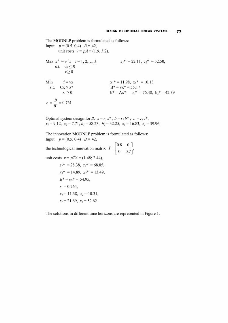
DESIGN OF OPTIMAL LINEAR SYSTEMS... 77
The MODNLP problem is formulated as follows: Input: p = (0.5, 0.4) B = 42, unit costs v = pA = (1.9, 3.2).
Max z i = c i x i = 1, 2,…, k z1* = 22.11, z2* = 52.50, s.t. vx ≤ B x ≥ 0
Min f = vx x1* = 11.98, x2* = 10.13 s.t. Cx ≥ z* B* = vx* = 55.17 x ≥ 0 b* = Ax* b1* = 76.48, b2* = 42.39
761.0*1 ==BBr
Optimal system design for B: x = r1 x* , b = r1 b* , z = r1 z*, x1 = 9.12, x2 = 7.71, b1 = 58.23, b2 = 32.25, z1 = 16.83, z2 = 39.96. The innovation MODNLP problem is formulated as follows: Input: p = (0.5, 0.4) B = 42,
the technological innovation matrix ⎥⎦
⎤⎢⎣
⎡=
7.0008.0
T ,
unit costs v = pTA = (1.48; 2.44),
z1* = 28.38, z2* = 68.85,
x1* = 14.89, x2* = 13.49,
B* = vx* = 54.95,
r1 = 0.764,
x1 = 11.38, x2 = 10.31,
z1 = 21.69, z2 = 52.62.
The solutions in different time horizons are represented in Figure 1.
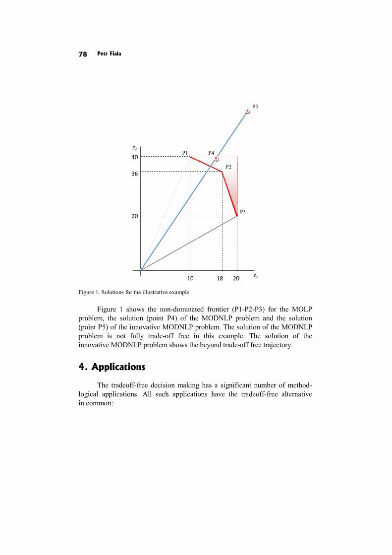
Petr Fiala 78
Figure 1. Solutions for the illustrative example
Figure 1 shows the non-dominated frontier (P1-P2-P3) for the MOLP
problem, the solution (point P4) of the MODNLP problem and the solution (point P5) of the innovative MODNLP problem. The solution of the MODNLP problem is not fully trade-off free in this example. The solution of the innovative MODNLP problem shows the beyond trade-off free trajectory.
4. Applications
The tradeoff-free decision making has a significant number of method-logical applications. All such applications have the tradeoff-free alternative in common:
P5
P1 P4
P2 PP
P3
40
20
10 18 20
36
z1
z2
P2
DESIGN OF OPTIMAL LINEAR SYSTEMS... 79
– Compromise programming – minimize distance from the ideal point. – Risk management – portfolio selection – tradeoffs between investment
returns and investment risk. – Game theory – win-win solutions. – Added value – value for the producer and value for the customer – both must
benefit. There are real applications of the De Novo approach. For example, the
production plan for an actual production system is defined taking into account financial constraints and given objective functions [Babic and Pavic 1996]. The paper [Zhang et al. 2009] presents an Inexact DNP approach for the design of optimal water-resources-management systems under uncertainty. Optimal supplies of good-quality water are obtained with different revenue targets of municipal–industrial–agricultural competition under a given budget taken into account.
In the next part a supply chain design problem is formulated. Supply chain management has generated a substantial amount of interest from both managers and researchers. Supply chain management is now seen as a governing element in strategy and as an effective way of creating value for customers. A supply chain is defined as a system of suppliers, manufacturers, distributors, retailers and customers where material, financial and information flows connect participants in both directions [see for example Fiala 2005]. There are many concepts and strategies applied to the design and management of supply chains. The fundamental decisions to be made during the design phase are the location of facilities and the capacity allocated to these facilities. An approach to designing an economically optimal supply chain is to develop and solve a mathematical programming model. A mathematical program determines the ideal locations for each facility and allocates the activity to each facility so that the costs are minimized and the constraints of meeting the customer demand and the facility capacity are satisfied. A general form of the model for the supply chain design is given below.
Model
Our model of a supply chain consists of 4 layers with m suppliers, S1, S2, … Sm, n potential producers, P1, P2, … Pn, p potential distributors, D1, D2, … Dp, and r customers, C1, C2, … Cn.
The following notation is used: ai = annual supply capacity of supplier i, bj = annual potential capacity of producer j,

Petr Fiala 80
wk = annual potential capacity of distributor k,
dl = annual demand of customer l, Pjf = fixed cost of potential producer j, D
kf = fixed cost of potential distributor k, Sijc = unit transportation cost from Si to Pj, Pjkc = unit transportation cost from Pj to Dk, Dklc = unit transportation cost from Dk to Cl, Sijt = unit transportation time from Si to Pj, Pjkt = unit transportation time from Pj to Dk, Dklt = unit transportation time from Dk to Cl, Sijx = number of units transported from Si to Pj, Pjkx = number of units transported from Pj to Dk, Dklx = number of units transported from Dk to Cl, Pjy = bivalent variable for build-up of fixed capacity of producer j, Dky = bivalent variable for build-up of fixed capacity of producer k.
With this notation the problem can be formulated as follows: The model has two objectives. The first one expresses the minimizing of total costs. The second one expresses the minimizing of total delivery time.
Min
11 1 1 1 1 1 1 1
p p pn m n n rP P D D S S P P D Dj j k k ij ij jk jk kl kl
j k i j j k k l
z f y f y c x c x c x= = = = = = = =
= + + + +∑ ∑ ∑∑ ∑∑ ∑∑
Min
21 1 1 1 1 1
p pm n n rS S P P D Dij ij jk jk kl kl
i j j k k l
z t x t x t x= = = = = =
= + +∑∑ ∑∑ ∑∑
Subject to the following constraints: – the amount sent from the supplier to the producers cannot exceed the
supplier’s capacity
,
1
1, 2, ..., ,n
ij ij
x a i m=
≤ =∑
DESIGN OF OPTIMAL LINEAR SYSTEMS... 81
– the amount produced by the producer cannot exceed the producer’s capacity
1, 1, 2, ..., ,
p
jk j jk
x b y j n=
≤ =∑
– the amount shipped from the distributor should not exceed the distributor’s capacity
1, 1, 2, ..., ,
r
kl k kl
x w y k p=
≤ =∑
– the amount shipped to the customer must equal the customer’s demand
1, 1, 2, ..., ,
p
kl lk
x d l r=
= =∑
– the amount shipped out of producers cannot exceed units received from suppliers
1 10, 1, 2, ..., ,
pm
ij jki k
x x j n= =
− ≥ =∑ ∑
– the amount shipped out of the distributors cannot exceed quantity received from the producers
1 1
0, 1, 2, ..., ,n r
jk klj l
x x k p= =
− ≥ =∑ ∑
– binary and non-negativity constraints
{ }, 0,1 ,
, , 0, 1, 2, ..., , 1, 2, ..., , 1, 2, ..., , 1, 2, ..., .j k
ij jk kl
Y
x x x i m j n k p l r
∈
≥ = = = = The formulated model is a multi-objective linear programming problem. The problem can be solved by an MOLP method.
The De Novo approach can be useful in the design of the supply chain. Only a partial relaxation of constraints is adopted. Producer and distributor capacities are relaxed. Unit costs for capacity build-up are computed:
PjP
jj
fp
b= = cost of unit capacity of potential producer j,
DD kk
k
fpw
= = cost of unit capacity of potential distributor k.

Petr Fiala 82
Variables for build-up capacities are introduced: Pju = variable for flexible capacity of producer j, Dku = variable for flexible capacity of producer k.
The constraints for non-exceeding producer and distributor fixed capacities are replaced by the flexible capacity constraints and the budget constraint:
10, 1, 2, ..., ,
pP
jk jk
x u j n=
− ≤ =∑
10, 1, 2, ..., ,
rD
kl kl
x u k p=
− ≤ =∑
1 1
.pn
P P D Dj j k k
j k
p u p u B= =
+ ≤∑ ∑
Example 2 An example of the supply chain with 3 potential producers, 3 potential
distributors, and 3 customers was tested. Data are presented in Tables 1, 2 and 3.
Table 1
Unit transportation costs
Pijc
D1 D2 D3
Djkc C1 C2 C3
P1 5 3 8 D1 3 1 4 P2 3 6 2 D2 6 7 2 P3 8 4 5 D3 5 4 8
Table 2
Unit transportation time
Pijc
D1 D2 D3
Djkc C1 C2 C3
P1 4 2 3 D1 6 1 2 P2 3 2 2 D2 3 2 5 P3 1 5 3 D3 1 4 2
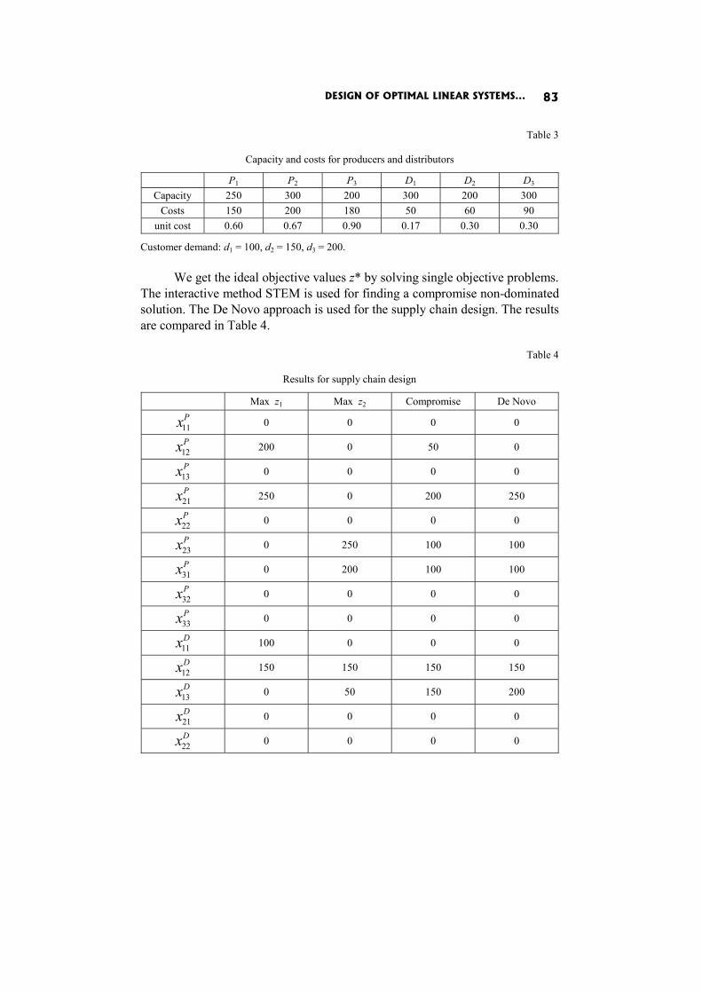
DESIGN OF OPTIMAL LINEAR SYSTEMS... 83
Table 3
Capacity and costs for producers and distributors
P1 P2 P3 D1 D2 D3 Capacity 250 300 200 300 200 300
Costs 150 200 180 50 60 90 unit cost 0.60 0.67 0.90 0.17 0.30 0.30
Customer demand: d1 = 100, d2 = 150, d3 = 200. We get the ideal objective values z* by solving single objective problems.
The interactive method STEM is used for finding a compromise non-dominated solution. The De Novo approach is used for the supply chain design. The results are compared in Table 4.
Table 4
Results for supply chain design
Max z1 Max z2 Compromise De Novo
11Px 0 0 0 0
12Px 200 0 50 0
13Px 0 0 0 0
21Px 250 0 200 250
22Px 0 0 0 0
23Px 0 250 100 100
31Px 0 200 100 100
32Px 0 0 0 0
33Px 0 0 0 0
11Dx 100 0 0 0
12Dx 150 150 150 150
13Dx 0 50 150 200
21Dx 0 0 0 0
22Dx 0 0 0 0
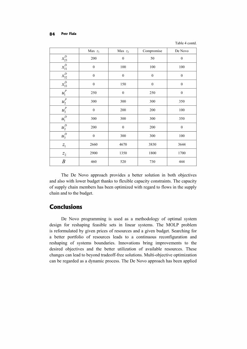
Petr Fiala 84
Table 4 contd.
Max z1 Max z2 Compromise De Novo
23Dx 200 0 50 0
31Dx 0 100 100 100
32Dx 0 0 0 0
33Dx 0 150 0 0
1Pu 250 0 250 0
2Pu 300 300 300 350
3Pu 0 200 200 100
1Du 300 300 300 350
2Du 200 0 200 0
3Du 0 300 300 100
1z 2660 4670 3830 3644
2z 2900 1350 1800 1700
B 460 520 730 444
The De Novo approach provides a better solution in both objectives
and also with lower budget thanks to flexible capacity constraints. The capacity of supply chain members has been optimized with regard to flows in the supply chain and to the budget.
Conclusions
De Novo programming is used as a methodology of optimal system design for reshaping feasible sets in linear systems. The MOLP problem is reformulated by given prices of resources and a given budget. Searching for a better portfolio of resources leads to a continuous reconfiguration and reshaping of systems boundaries. Innovations bring improvements to the desired objectives and the better utilization of available resources. These changes can lead to beyond tradeoff-free solutions. Multi-objective optimization can be regarded as a dynamic process. The De Novo approach has been applied
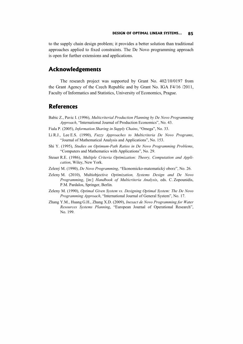
DESIGN OF OPTIMAL LINEAR SYSTEMS... 85
to the supply chain design problem; it provides a better solution than traditional approaches applied to fixed constraints. The De Novo programming approach is open for further extensions and applications.
Acknowledgements
The research project was supported by Grant No. 402/10/0197 from the Grant Agency of the Czech Republic and by Grant No. IGA F4/16 /2011, Faculty of Informatics and Statistics, University of Economics, Prague.
References
Babic Z., Pavic I. (1996), Multicriterial Production Planning by De Novo Programming Approach, “International Journal of Production Economics”, No. 43.
Fiala P. (2005), Information Sharing in Supply Chains, “Omega”, No. 33. Li R.J., Lee E.S. (1990), Fuzzy Approaches to Multicriteria De Novo Programs,
“Journal of Mathematical Analysis and Applications”, No. 153. Shi Y. (1995), Studies on Optimum-Path Ratios in De Novo Programming Problems,
“Computers and Mathematics with Applications”, No. 29. Steuer R.E. (1986), Multiple Criteria Optimization: Theory, Computation and Appli-
cation, Wiley, New York. Zelený M. (1990), De Novo Programming, “Ekonomicko-matematický oborz”, No. 26. Zeleny M. (2010), Multiobjective Optimization, Systems Design and De Novo
Programming, [in:] Handbook of Multicriteria Analysis, eds. C. Zopounidis, P.M. Pardalos, Springer, Berlin.
Zeleny M. (1990), Optimal Given System vs. Designing Optimal System: The De Novo Programming Approach, “International Journal of General System”, No. 17.
Zhang Y.M., Huang G.H., Zhang X.D. (2009), Inexact de Novo Programming for Water Resources Systems Planning, “European Journal of Operational Research”, No. 199.

Dorota Górecka
SENSITIVITY AND ROBUSTNESS ANALYSIS OF SOLUTIONS OBTAINED IN THE EUROPEAN PROJECTS’ RANKING PROCESS
Abstract
After entering the European Union on 1 May 2004 Poland has become eligible to benefit from the EU Structural Funds and the Cohesion Fund and projects co-financed by these means have become a crucial instrument supporting restructuring and modernization of Polish economy. Total financial assistance granted to Poland for the previous (2004-2006) and present (2007-2013) programming periods amounts to over 80 billion euro. An efficient allocation of these subsidies depends, among other things, on proper choice of projects that are going to be co-financed, which can be made with the aid of such multi-criteria techniques as ORESTE, EVAMIX, PROMETHEE II, EXPROM II or modified BIPOLAR method.
In the paper sensitivity and robustness analysis of solutions obtained with the help of the above-mentioned methods will be carried out. It will enable to show the influence of the information delivered by the decision-makers and choices made by them during the decision aiding process on the final European projects’ ranking. In a real-life example concerning this issue 16 applications for project co-financing by the European Regional Development Fund submitted to Measure 1.2 Environmental protection infrastructure in one of Polish voivodships in the programming period 2004-2006 will be used.
Keywords
Multi-criteria decision aiding methods: ORESTE, EVAMIX, PROMETHEE II, EXPROM II, modified BIPOLAR method, stochastic dominance rules, sensitivity and robustness analysis.
Introduction
European regional policy is currently one of the crucial factors in strengthening the socio-economic development of Poland and other European Union countries, especially those that entered the EU in 2004 and 2007, whose
SENSITIVITY AND ROBUSTNESS ANALYSIS... 87
economies have lagged far behind the economies of the old Member States of EU-15 and whose needs in the areas of environment, infrastructure, research and innovation, industry, services and SMEs are truly significant [Górecka 2011b].
Regional policy helps to reduce disparities between countries, increase the regions’ competitiveness and attractiveness, improve the employment prospects and support innovation and development of the knowledge society as well as environmental protection. Moreover, it strengthens cross-border co-operation through financing concrete projects for regions, towns and their inhabitants.
In the previous programming period 2000-2006 over 233 billion EUR was earmarked for all regional instruments for the 15 old Member States. Moreover, around 24 billion EUR was allocated for the 10 new Member States for years 2004-2006, not to mention 22 billion EUR granted for pre-accession aid. In the present programming period 2007-2013 cohesion policy benefits from total allocation of about 347 billion EUR, which represents nearly 36% of the entire Union’s budget.
Because of the enormous amount of money devoted to the structural aid it is crucially important to allocate the means in the most effective way possible. And that depends, among other things, on the proper choice of projects to be co-financed. In order to help the decision-makers in this challenging and difficult task multi-criteria decision aiding techniques, which refers to making decision in the presence of multiple, usually conflicting criteria, should be applied as evaluation of the European projects requires taking into account many diverse aspects: economic, financial, environmental, ecological, technical, technological, social and legal [Górecka 2011b].
Sensitivity and robustness analysis of the obtained solutions to the changes of the parameters of the preference model is in the case of projects applying for co-financing from the European Union funds quite a risky undertaking – in the extreme case it may lead even to undermining the decisions taken as a result of the proceedings conducted, i.e. to contesting the list of projects selected for funding. However, such analysis will be carried out for the purposes of this paper, primarily to demonstrate the importance of the quality of both the information acquired from the participants of the decision-making process and choices made by the decision-makers during the decision-aiding process, and the extent of their influence on the final ranking of projects [Górecka 2011a1].
1 This publication is devoted to the sensitivity and robustness analysis of solutions obtained with the help
of the following MCDA techniques: PROMETHEE II with stochastic dominance rules, EXPROM II with stochastic dominance rules and modified BIPOLAR method with stochastic dominance rules.
Dorota Górecka 88
1. Sensitivity and robustness analysis
When solving real decision-making problems decision-makers and analysts encounter problems related to the imperfection of knowledge. This deficiency has several different causes but invariably leads to assigning arbitrary values to the certain parameters of models and algorithms used in the decision-making process. In this case parameters are very broadly defined and include both the data in the classical sense of the word and information about values and beliefs of the participants of the decision-making process as well as information regarding technical issues related to the algorithms operation. In the multi-criteria methods based on the outranking relation, among which the ELECTRE and PROMETHEE methods stand out, doubts resulting from the imperfection of available data may concern both parameters related to the modelling of preferences (weights, thresholds or categories profiles) and technical parameters such as, for example, the cutting level λ [Figueira et al. 2005, p. 149]. Since it is difficult to expect that the participants of the decision-making process will easily define the values of parameters, therefore each of their permissible combinations should be treated as a “working hypothesis”. The problem is that different “working hypothesis” may lead to different results [Dias and Climaco 1999, p. 74].
In practice, a reference system composed of central values of the parameters is often defined and on this basis the calculations are carried out, whose results are used to prepare recommendations for the decision-makers. Subsequently the sensitivity of the solution to changes in the values of the parameters is examined. This analysis is usually performed for each parameter separately (ignoring possible interdependencies among them). It allows you to define the scope of the changes in the values of the parameters which make no impact on the solution designated earlier and also specify these parameters, whose values, when varying from the central positions, particularly strongly affect the outcome [Figueira et al. 2005, p. 149-150].
As an alternative for the sensitivity analysis the robustness analysis of the obtained solutions to changes in the values of the parameters may be considered. In this case the problem is defined as follows: assuming that the role of the analyst is to build such recommendations that will prove correct for the possibly wide range of the parameter values, we want to obtain

SENSITIVITY AND ROBUSTNESS ANALYSIS... 89
information on the solutions proposed, depending on the values of the para-meters. Thus, we are interested in whether and how the solution of the problem will be changing with modification of the parameters within the sets of their admissible values.
The concept of robustness was introduced by Roy [Roy and Hugonnard 1982, p. 301-312; Roy 1998, p. 141-160] who has formulated a definition of the robust conclusion describing it as a formalized premise that is true for all plausible combinations of parameter values. Dias and Climaco, starting with the definition given by Roy, have distinguished the following types of the robust conclusions [Dias and Climaco 1999, p. 75]: – an absolute robust conclusion – a premise intrinsic to one of the examined
variants, which is valid for all acceptable combinations of parameter values; in the case of additive aggregation model the absolute conclusion may be “for example as follows: “the assessment of the variant ia is less than 0,5”;
– a relative binary robust conclusion – a premise concerning a pair of variants, which is true for all possible values of parameters; for example: “ ia outranks ja with credibility greater than 0,8”;
– a relative unary robust conclusion – a premise concerning one variant but referring to others, binding for each admissible combination of parameter values; for example: “ ia is placed on one of the top three positions in the ranking”.
2. The proposed procedure of appraising and selecting European projects
Meeting the need to improve the system of evaluation and selection of applications for project co-financing by the European Union funds and taking into account advantages and disadvantages of different multi-criteria decision aiding methods2, the procedure composed of the following elements has been proposed to aid the choice of European projects: – identification of the participants of the decision-making process; – selection of the criteria and determination of their weights with the help of:
2 [See Górecka 2010, p. 105-108].
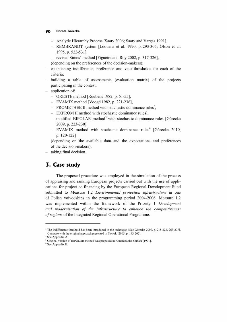
Dorota Górecka 90
– Analytic Hierarchy Process [Saaty 2006; Saaty and Vargas 1991], – REMBRANDT system [Lootsma et al. 1990, p. 293-305; Olson et al.
1995, p. 522-531], – revised Simos’ method [Figueira and Roy 2002, p. 317-326], (depending on the preferences of the decision-makers);
– establishing indifference, preference and veto thresholds for each of the criteria;
– building a table of assessments (evaluation matrix) of the projects participating in the contest;
– application of: – ORESTE method [Roubens 1982, p. 51-55], – EVAMIX method [Voogd 1982, p. 221-236], – PROMETHEE II method with stochastic dominance rules3, – EXPROM II method with stochastic dominance rules4, – modified BIPOLAR method5 with stochastic dominance rules [Górecka
2009, p. 223-230], – EVAMIX method with stochastic dominance rules6 [Górecka 2010,
p. 120-122] (depending on the available data and the expectations and preferences of the decision-makers);
– taking final decision.
3. Case study
The proposed procedure was employed in the simulation of the process of appraising and ranking European projects carried out with the use of appli-cations for project co-financing by the European Regional Development Fund submitted to Measure 1.2 Environmental protection infrastructure in one of Polish voivodships in the programming period 2004-2006. Measure 1.2 was implemented within the framework of the Priority 1 Development and modernisation of the infrastructure to enhance the competitiveness of regions of the Integrated Regional Operational Programme.
3 The indifference threshold has been introduced to the technique. [See Górecka 2009, p. 218-223, 263-277].
Compare with the original approach presented in Nowak [2005, p. 193-202]. 4 See Appendix A. 5 Original version of BIPOLAR method was proposed in Konarzewska-Gubała [1991]. 6 See Appendix B.
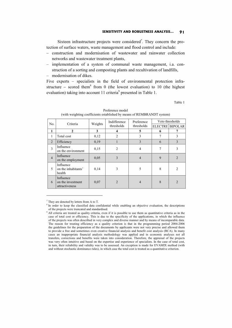
SENSITIVITY AND ROBUSTNESS ANALYSIS... 91
Sixteen infrastructure projects were considered7. They concern the pro-tection of surface waters, waste management and flood control and include: – construction and modernisation of wastewater and rainwater collection
networks and wastewater treatment plants, – implementation of a system of communal waste management, i.a. con-
struction of a sorting and composting plants and recultivation of landfills, – modernisation of dikes. Five experts − specialists in the field of environmental protection infra- structure − scored them8 from 0 (the lowest evaluation) to 10 (the highest evaluation) taking into account 11 criteria9 presented in Table 1.
Table 1
Preference model
(with weighting coefficients established by means of REMBRANDT system)
No. Criteria Weights Indifference thresholds
Preference thresholds
Veto thresholds ELECTRE BIPOLAR
1 2 3 4 5 6 7 1 Total cost 0,12 2 3 7 3 2 Efficiency 0,19 1 3 6 3
3 Influence on the environment 0,15 2 4 7 3
4 Influence on the employment 0,05 3 4 9 2
5 Influence on the inhabitants’ health
0,14 3 5 8 2
6 Influence on the investment attractiveness
0,07 2 4 8 2
7 They are denoted by letters from A to T. 8 In order to keep the classified data confidential while enabling an objective evaluation, the descriptions
of the projects were truncated and standardised. 9 All criteria are treated as quality criteria, even if it is possible to use them as quantitative criteria as in the
case of total cost or efficiency. This is due to the specificity of the applications, in which the influence of the projects was often described in very complex and diverse manner and by means of incomparable data. The reason for treating efficiency as a quality criterion is that in the programming period 2004-2006 the guidelines for the preparation of the documents by applicants were not very precise and allowed them to provide a free and sometimes even creative financial analysis and benefit cost analysis (BCA). In many cases an inappropriate financial analysis methodology was applied and in economic analyses not all transfers, corrections and benefits were taken into consideration. Therefore, the appraisal of the projects was very often intuitive and based on the expertise and experience of specialists. In the case of total cost, in turn, their reliability and validity was to be assessed. An exception is made for EVAMIX method (with and without stochastic dominance rules), in which case the total cost is treated as a quantitative criterion.
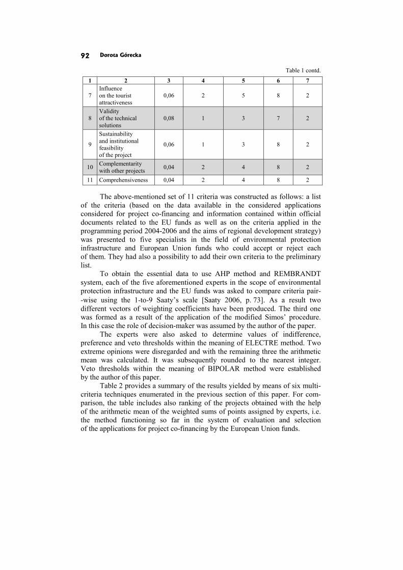
Dorota Górecka 92
Table 1 contd.
1 2 3 4 5 6 7
7 Influence on the tourist attractiveness
0,06 2 5 8 2
8 Validity of the technical solutions
0,08 1 3 7 2
9
Sustainability and institutional feasibility of the project
0,06 1 3 8 2
10 Complementarity with other projects 0,04 2 4 8 2
11 Comprehensiveness 0,04 2 4 8 2
The above-mentioned set of 11 criteria was constructed as follows: a list of the criteria (based on the data available in the considered applications considered for project co-financing and information contained within official documents related to the EU funds as well as on the criteria applied in the programming period 2004-2006 and the aims of regional development strategy) was presented to five specialists in the field of environmental protection infrastructure and European Union funds who could accept or reject each of them. They had also a possibility to add their own criteria to the preliminary list.
To obtain the essential data to use AHP method and REMBRANDT system, each of the five aforementioned experts in the scope of environmental protection infrastructure and the EU funds was asked to compare criteria pair- -wise using the 1-to-9 Saaty’s scale [Saaty 2006, p. 73]. As a result two different vectors of weighting coefficients have been produced. The third one was formed as a result of the application of the modified Simos’ procedure. In this case the role of decision-maker was assumed by the author of the paper.
The experts were also asked to determine values of indifference, preference and veto thresholds within the meaning of ELECTRE method. Two extreme opinions were disregarded and with the remaining three the arithmetic mean was calculated. It was subsequently rounded to the nearest integer. Veto thresholds within the meaning of BIPOLAR method were established by the author of this paper.
Table 2 provides a summary of the results yielded by means of six multi-criteria techniques enumerated in the previous section of this paper. For com-parison, the table includes also ranking of the projects obtained with the help of the arithmetic mean of the weighted sums of points assigned by experts, i.e. the method functioning so far in the system of evaluation and selection of the applications for project co-financing by the European Union funds.
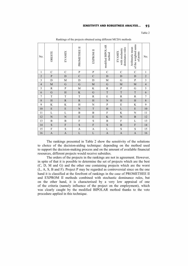
SENSITIVITY AND ROBUSTNESS ANALYSIS... 93
Table 2
Rankings of the projects obtained using different MCDA methods
No.
OR
ESTE
EVA
MIX
PRO
MET
HEE
II
EXPR
OM
II
mod
ified
BIP
OLA
R
met
hod
EVA
MIX
w
ith st
ocha
stic
do
min
ance
rule
s
Arit
hmet
ic m
ean
of
the
wei
ghte
d su
ms
of p
oint
s
No.
1 C C P P C C C 1 2 P D C C D D D 2 3 D M D D M G P 3 4 M G G M G M M 4 5 R P M K R P G 5 6 G H K G T T T 6 7 T T T R E R R 7 8 H R R H N H H 8 9 K K H N P E K 9
10 E E N T H L E 10 11 L L B B F K N 11 12 N N E E K N B 12 13 B B F S B F L 13 14 S F S F S B F 14 15 F S A A L S S 15 16 A A L L A A A 16
The rankings presented in Table 2 show the sensitivity of the solutions
to choice of the decision-aiding technique: depending on the method used to support the decision-making process and on the amount of available financial resources, different projects would receive subsidies.
The orders of the projects in the rankings are not in agreement. However, in spite of that it is possible to determine the set of projects which are the best (C, D, M and G) and the other one containing projects which are the worst (L, A, S, B and F). Project P may be regarded as controversial since on the one hand it is classified at the forefront of rankings in the case of PROMETHEE II and EXPROM II methods combined with stochastic dominance rules, but on the other hand, it is characterised by a very low appraisal of one of the criteria (namely influence of the project on the employment), which was clearly caught by the modified BIPOLAR method thanks to the veto procedure applied in this technique.
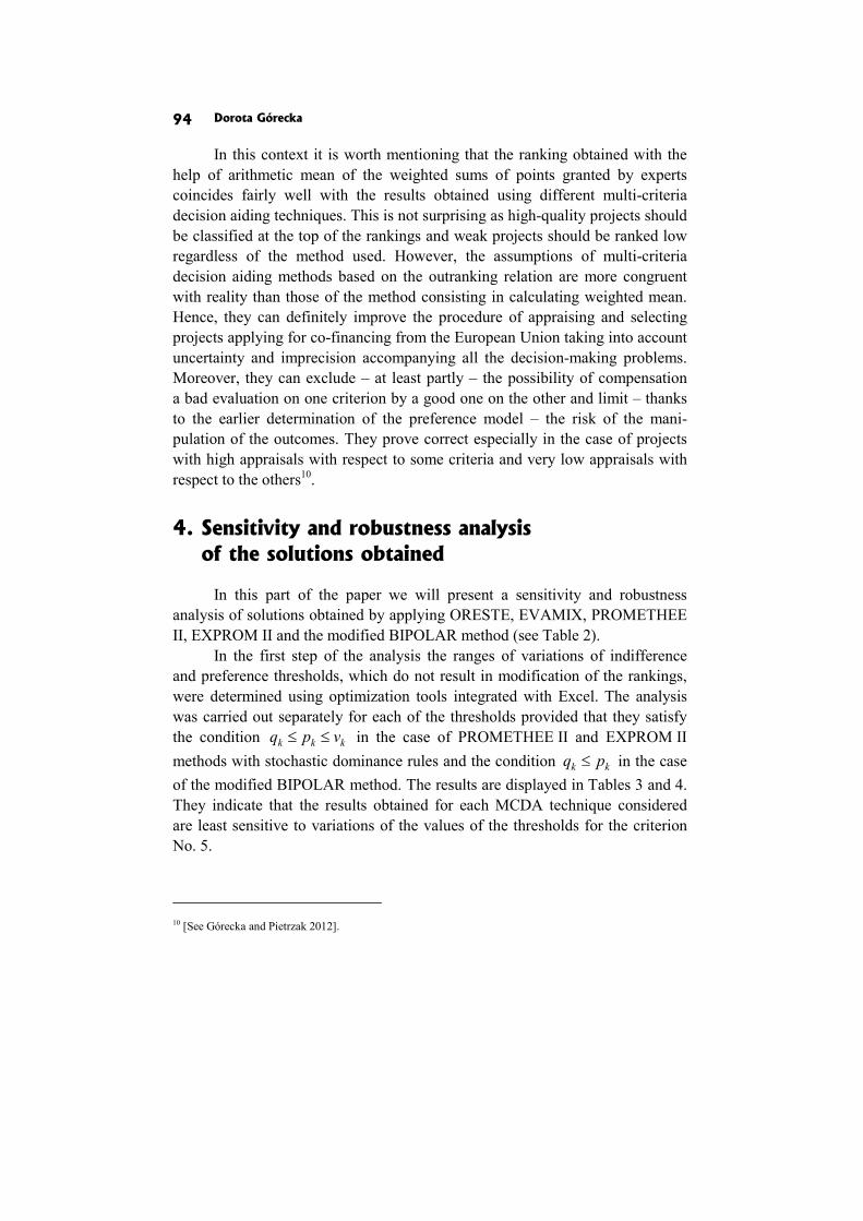
Dorota Górecka 94
In this context it is worth mentioning that the ranking obtained with the help of arithmetic mean of the weighted sums of points granted by experts coincides fairly well with the results obtained using different multi-criteria decision aiding techniques. This is not surprising as high-quality projects should be classified at the top of the rankings and weak projects should be ranked low regardless of the method used. However, the assumptions of multi-criteria decision aiding methods based on the outranking relation are more congruent with reality than those of the method consisting in calculating weighted mean. Hence, they can definitely improve the procedure of appraising and selecting projects applying for co-financing from the European Union taking into account uncertainty and imprecision accompanying all the decision-making problems. Moreover, they can exclude – at least partly – the possibility of compensation a bad evaluation on one criterion by a good one on the other and limit – thanks to the earlier determination of the preference model – the risk of the mani-pulation of the outcomes. They prove correct especially in the case of projects with high appraisals with respect to some criteria and very low appraisals with respect to the others10.
4. Sensitivity and robustness analysis of the solutions obtained
In this part of the paper we will present a sensitivity and robustness analysis of solutions obtained by applying ORESTE, EVAMIX, PROMETHEE II, EXPROM II and the modified BIPOLAR method (see Table 2).
In the first step of the analysis the ranges of variations of indifference and preference thresholds, which do not result in modification of the rankings, were determined using optimization tools integrated with Excel. The analysis was carried out separately for each of the thresholds provided that they satisfy the condition kkk vpq ≤≤ in the case of PROMETHEE II and EXPROM II methods with stochastic dominance rules and the condition kk pq ≤ in the case of the modified BIPOLAR method. The results are displayed in Tables 3 and 4. They indicate that the results obtained for each MCDA technique considered are least sensitive to variations of the values of the thresholds for the criterion No. 5.
10 [See Górecka and Pietrzak 2012].

SENSITIVITY AND ROBUSTNESS ANALYSIS... 95
Table 3
Ranges of variations of the indifference thresholds values
No. Criteria
q min
q original
q max
PRO
MET
HEE
II
EXPR
OM
II
BIP
OLA
R
BIP
OLA
R
EXPR
OM
II
PRO
MET
HEE
II
1 Total cost 1,974 1,596 1,788 2 2,225 2,143 2,132 2 Efficiency 0,946 0,945 0,077 1 1,272 1,002 1,067
3 Influence on the environment 1,501 1,641 1,715 2 2,214 2,201 2,106
4 Influence on the employment 2,843 2,998 3,000 3 3,655 3,306 3,079
5 Influence on the inhabitants’ health
2,122 2,196 2,412 3 5,000 5,000 5,000
6 Influence on the investment attractiveness
1,432 1,998 1,539 2 2,180 2,246 2,081
7 Influence on the tourist attractiveness 0,702 1,998 1,420 2 2,159 2,907 2,080
8 Validity of the technical solutions
0,930 0,995 0,000 1 1,379 1,115 1,330
9
Sustainability and institutional feasibility of the project
0,954 0,979 0,372 1 2,529 1,300 3,000
10 Complementarity with other projects 1,702 0,877 1,415 2 2,836 2,002 2,248
11 Comprehensiveness 1,812 1,996 1,509 2 3,733 3,383 2,735
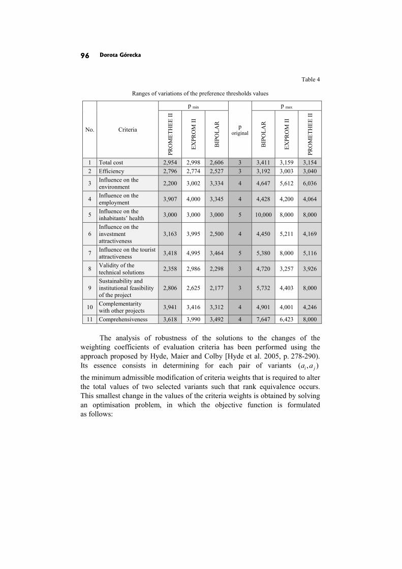
Dorota Górecka 96
Table 4
Ranges of variations of the preference thresholds values
No. Criteria
p min
p original
p max
PRO
MET
HEE
II
EXPR
OM
II
BIP
OLA
R
BIP
OLA
R
EXPR
OM
II
PRO
MET
HEE
II
1 Total cost 2,954 2,998 2,606 3 3,411 3,159 3,154 2 Efficiency 2,796 2,774 2,527 3 3,192 3,003 3,040
3 Influence on the environment 2,200 3,002 3,334 4 4,647 5,612 6,036
4 Influence on the employment 3,907 4,000 3,345 4 4,428 4,200 4,064
5 Influence on the inhabitants’ health 3,000 3,000 3,000 5 10,000 8,000 8,000
6 Influence on the investment attractiveness
3,163 3,995 2,500 4 4,450 5,211 4,169
7 Influence on the tourist attractiveness 3,418 4,995 3,464 5 5,380 8,000 5,116
8 Validity of the technical solutions 2,358 2,986 2,298 3 4,720 3,257 3,926
9 Sustainability and institutional feasibility of the project
2,806 2,625 2,177 3 5,732 4,403 8,000
10 Complementarity with other projects 3,941 3,416 3,312 4 4,901 4,001 4,246
11 Comprehensiveness 3,618 3,990 3,492 4 7,647 6,423 8,000 The analysis of robustness of the solutions to the changes of the
weighting coefficients of evaluation criteria has been performed using the approach proposed by Hyde, Maier and Colby [Hyde et al. 2005, p. 278-290). Its essence consists in determining for each pair of variants ),( ji aa the minimum admissible modification of criteria weights that is required to alter the total values of two selected variants such that rank equivalence occurs. This smallest change in the values of the criteria weights is obtained by solving an optimisation problem, in which the objective function is formulated as follows:

SENSITIVITY AND ROBUSTNESS ANALYSIS... 97
∑=
−=n
kkkE wwd
1
2)'(min , .,...,1 nk =
The aim is therefore to minimise a distance metric that provides the numerical measure to the amount of dissimilarity between the initial weights of the criteria kw and the optimised criteria weights kw' . The Euclidean distance has been selected as the most commonly used.
A set of constraints takes the following form:
∑ ∑= =
==n
k
n
kkk ww
1 1
1' , ,,...,1 nk =
,0', >kk ww
gkk
dk www ≤≤ ' , ,,...,1 nk =
where dkw and g
kw are the lower and upper limits, respectively, of the values of the weighting coefficients assigned to each of the evaluation criteria kf .
Applying the optimised criteria weighs should cause the total values of two variants being assessed to be equal, thus we have in addition:
).(')(' ji aa φφ =
As a result of solving the non-linear programming task presented above the values of the minimum Euclidean distance for all pairs of variants are obtained. They can be presented in the form of a matrix.
In some situations one of the variants is always classified higher in ranking than the other, regardless of the values of the modified parameters. In this case, the ordering of these two variants – because of the insensitivity to variation of parameters – is called robust. Much more often, however, we have to deal with the situation, in which there are at least a few different combinations of the weighting coefficients for which ).(')(' ji aa φφ = Setting the smallest overall modification of the criteria weights allowing two variants to achieve the same position in ranking, enables determining whether their ordering is robust or not. Large values of the minimum Euclidean distance mean that one of the variants is generally better than the other, regardless of the values of the parameters changing within the range given by the decision- -maker. If, on the other hand, the minimum Euclidean distances are small, minor changes in the values of the parameters will cause rank equivalence of variants being considered, thus their ordering may be concluded to be sensitive to the criteria weights [Hyde et al. 2005, p. 281-282].
Dorota Górecka 98
In the analysis performed the eight highest-ranked European projects in the orderings obtained with the help of EVAMIX method without stochastic dominance, PROMETHEE II technique with stochastic dominance rules and the modified BIPOLAR method have been taken into account. It has been assumed that the values of the weighting coefficients for evaluation criteria are within the following limits:
Table 5
The permissible range of variability in the values
of the weighting coefficients for project evaluation criteria
No. Criteria Coefficients of importance
w min w original w max 1 Total cost 0,05 0,12 0,20 2 Efficiency 0,10 0,19 0,20 3 Influence on the environment 0,10 0,15 0,20 4 Influence on the employment 0,03 0,05 0,10 5 Influence on the inhabitants’ health 0,10 0,14 0,20 6 Influence on the investment attractiveness 0,03 0,07 0,10 7 Influence on the tourist attractiveness 0,03 0,06 0,10 8 Validity of the technical solutions 0,03 0,08 0,10
9 Sustainability and institutional feasibility of the project 0,03 0,06 0,10
10 Complementarity with other projects 0,03 0,04 0,10 11 Comprehensiveness 0,03 0,04 0,10
The values of the minimum Euclidean distance Ed for pairs of con-
sidered projects contained in Tables 6, 7 and 8 signify that the final rankings are not robust to changes in the criteria weights – in some cases only small modifications of the starting values are required for rank equivalence between the two examined variants.
The results of using the distance-based analysis approach for 28 pairs of projects also indicate that although the obtained solutions are sensitive to variations of input parameter values, the orderings of some projects are robust. For the acceptable ranges of weighting coefficients given in Table 5 in the case of: – EVAMIX method without stochastic dominance projects C and D
(not necessarily in that order) will always be superior to projects H, T and R (no feasible changes in criteria weights could be found); furthermore project C will be also superior to projects M, G and P;
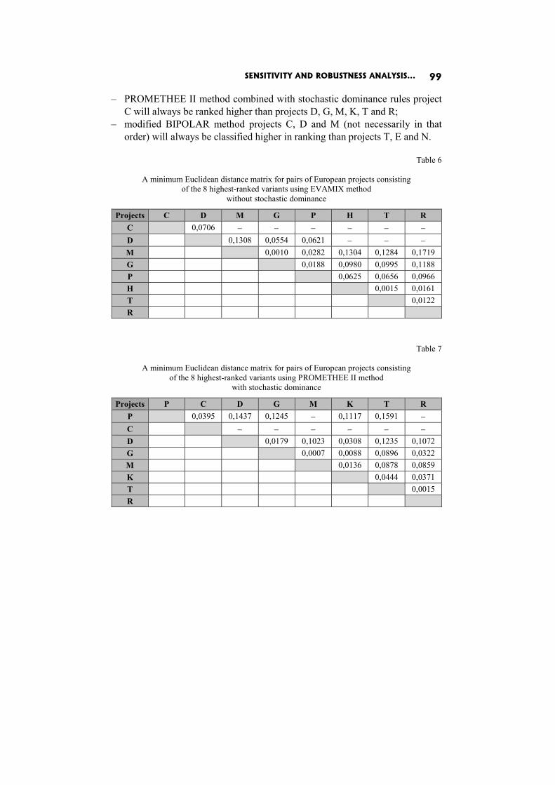
SENSITIVITY AND ROBUSTNESS ANALYSIS... 99
– PROMETHEE II method combined with stochastic dominance rules project C will always be ranked higher than projects D, G, M, K, T and R;
– modified BIPOLAR method projects C, D and M (not necessarily in that order) will always be classified higher in ranking than projects T, E and N.
Table 6
A minimum Euclidean distance matrix for pairs of European projects consisting
of the 8 highest-ranked variants using EVAMIX method without stochastic dominance
Projects C D M G P H T R C 0,0706 − − − − − − D 0,1308 0,0554 0,0621 − − − M 0,0010 0,0282 0,1304 0,1284 0,1719 G 0,0188 0,0980 0,0995 0,1188 P 0,0625 0,0656 0,0966 H 0,0015 0,0161 T 0,0122 R
Table 7
A minimum Euclidean distance matrix for pairs of European projects consisting of the 8 highest-ranked variants using PROMETHEE II method
with stochastic dominance
Projects P C D G M K T R P 0,0395 0,1437 0,1245 − 0,1117 0,1591 − C − − − − − − D 0,0179 0,1023 0,0308 0,1235 0,1072 G 0,0007 0,0088 0,0896 0,0322 M 0,0136 0,0878 0,0859 K 0,0444 0,0371 T 0,0015 R
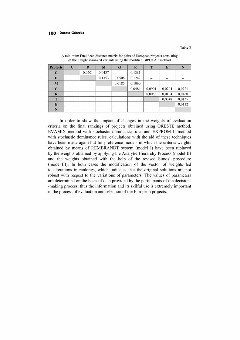
Dorota Górecka 100
Table 8
A minimum Euclidean distance matrix for pairs of European projects consisting
of the 8 highest-ranked variants using the modified BIPOLAR method
Projects C D M G R T E N C 0,0201 0,0437 − 0,1381 − − − D 0,1353 0,0506 0,1242 − − − M 0,0185 0,1060 − − − G 0,0484 0,0901 0,0704 0,0721 R 0,0088 0,0104 0,0460 T 0,0048 0,0135 E 0,0112 N
In order to show the impact of changes in the weights of evaluation
criteria on the final rankings of projects obtained using ORESTE method, EVAMIX method with stochastic dominance rules and EXPROM II method with stochastic dominance rules, calculations with the aid of these techniques have been made again but for preference models in which the criteria weights obtained by means of REMBRANDT system (model I) have been replaced by the weights obtained by applying the Analytic Hierarchy Process (model II) and the weights obtained with the help of the revised Simos’ procedure (model III). In both cases the modification of the vector of weights led to alterations in rankings, which indicates that the original solutions are not robust with respect to the variations of parameters. The values of parameters are determined on the basis of data provided by the participants of the decision- -making process, thus the information and its skilful use is extremely important in the process of evaluation and selection of the European projects.
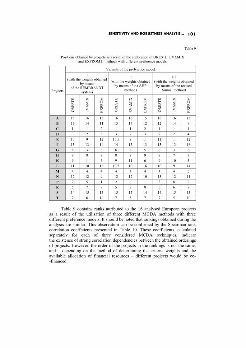
SENSITIVITY AND ROBUSTNESS ANALYSIS... 101
Table 9
Positions obtained by projects as a result of the application of ORESTE, EVAMIX
and EXPROM II methods with different preference models
Projects
Variants of the preference model I
(with the weights obtained by means
of the REMBRANDT system)
II (with the weights obtained
by means of the AHP method)
III (with the weights obtained
by means of the revised Simos’ method)
OR
ESTE
EVA
MIX
EXPR
OM
OR
ESTE
EVA
MIX
EXPR
OM
OR
ESTE
EVA
MIX
EXPR
OM
A 16 16 15 16 16 15 16 16 15 B 13 14 11 13 14 12 12 14 9 C 1 1 2 1 1 2 1 1 1 D 3 2 3 3 2 3 2 2 4 E 10 9 12 10,5 9 11 11 11 12 F 15 13 14 14 13 13 15 13 16 G 6 3 6 6 3 5 6 3 6 H 8 8 8 8 8 9 8 7 7 K 9 11 5 9 11 6 9 10 3 L 11 10 16 10,5 10 16 10 9 14 M 4 4 4 4 4 4 4 4 5 N 12 12 9 12 12 10 13 12 11 P 2 5 1 2 6 1 3 8 2 R 5 7 7 5 7 8 5 6 8 S 14 15 13 15 15 14 14 15 13 T 7 6 10 7 5 7 7 5 10
Table 9 contains ranks attributed to the 16 analysed European projects
as a result of the utilisation of three different MCDA methods with three different preference models. It should be noted that rankings obtained during the analysis are similar. This observation can be confirmed by the Spearman rank correlation coefficients presented in Table 10. These coefficients, calculated separately for each of three considered MCDA techniques, indicate the existence of strong correlation dependencies between the obtained orderings of projects. However, the order of the projects in the rankings is not the same, and – depending on the method of determining the criteria weights and the available allocation of financial resources – different projects would be co- -financed.
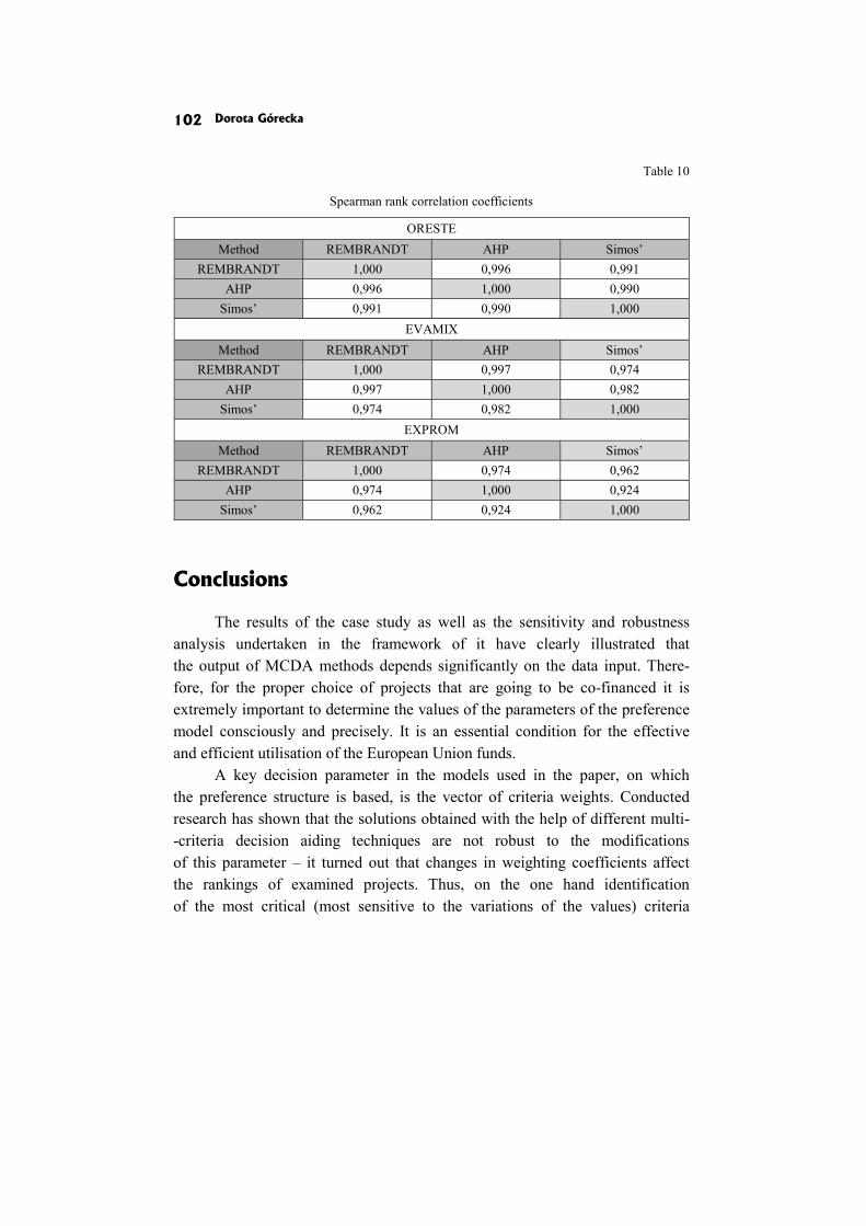
Dorota Górecka 102
Table 10
Spearman rank correlation coefficients
ORESTE Method REMBRANDT AHP Simos’
REMBRANDT 1,000 0,996 0,991 AHP 0,996 1,000 0,990
Simos’ 0,991 0,990 1,000 EVAMIX
Method REMBRANDT AHP Simos’ REMBRANDT 1,000 0,997 0,974
AHP 0,997 1,000 0,982 Simos’ 0,974 0,982 1,000
EXPROM Method REMBRANDT AHP Simos’
REMBRANDT 1,000 0,974 0,962 AHP 0,974 1,000 0,924
Simos’ 0,962 0,924 1,000
Conclusions
The results of the case study as well as the sensitivity and robustness analysis undertaken in the framework of it have clearly illustrated that the output of MCDA methods depends significantly on the data input. There-fore, for the proper choice of projects that are going to be co-financed it is extremely important to determine the values of the parameters of the preference model consciously and precisely. It is an essential condition for the effective and efficient utilisation of the European Union funds.
A key decision parameter in the models used in the paper, on which the preference structure is based, is the vector of criteria weights. Conducted research has shown that the solutions obtained with the help of different multi- -criteria decision aiding techniques are not robust to the modifications of this parameter – it turned out that changes in weighting coefficients affect the rankings of examined projects. Thus, on the one hand identification of the most critical (most sensitive to the variations of the values) criteria
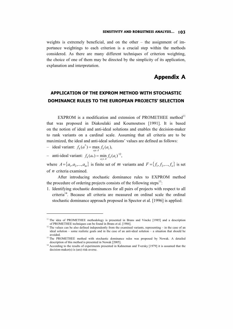
SENSITIVITY AND ROBUSTNESS ANALYSIS... 103
weights is extremely beneficial, and on the other – the assignment of im-portance weightings to each criterion is a crucial step within the methods considered. As there are many different techniques of criterion weighting, the choice of one of them may be directed by the simplicity of its application, explanation and interpretation.
Appendix A
APPLICATION OF THE EXPROM METHOD WITH STOCHASTIC
DOMINANCE RULES TO THE EUROPEAN PROJECTS’ SELECTION
EXPROM is a modification and extension of PROMETHEE method11 that was proposed in Diakoulaki and Koumoutsos [1991]. It is based on the notion of ideal and anti-ideal solutions and enables the decision-maker to rank variants on a cardinal scale. Assuming that all criteria are to be maximized, the ideal and anti-ideal solutions’ values are defined as follows: – ideal variant: ),(max)( *
ikAak afafi∈
=
– anti-ideal variant: )(min)( * ikAak afafi ∈
= 12,
where { }maaaA ,...,, 21= is finite set of m variants and { }nfffF ,...,, 21= is set of n criteria examined.
After introducing stochastic dominance rules to EXPROM method the procedure of ordering projects consists of the following steps13: 1. Identifying stochastic dominances for all pairs of projects with respect to all
criteria14. Because all criteria are measured on ordinal scale the ordinal stochastic dominance approach proposed in Spector et al. [1996] is applied:
11 The idea of PROMETHEE methodology is presented in Brans and Vincke [1985] and a description
of PROMETHEE techniques can be found in Brans et al. [1986]. 12 The values can be also defined independently from the examined variants, representing – in the case of an
ideal solution – some realistic goals and in the case of an anti-ideal solution – a situation that should be avoided.
13 The PROMETHEE method with stochastic dominance rules was proposed by Nowak. A detailed description of this method is presented in Nowak [2005].
14 According to the results of experiments presented in Kahneman and Tversky [1979] it is assumed that the decision-maker(s) is (are) risk-averse.
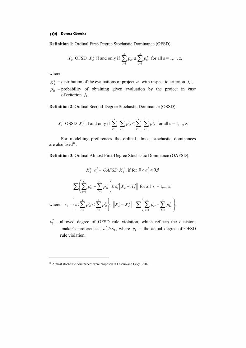
Dorota Górecka 104
Definition 1: Ordinal First-Degree Stochastic Dominance (OFSD):
ikX OFSD j
kX if and only if ∑∑==
≤s
l
jkl
s
l
ikl pp
11 for all s = 1,..., z,
where: ikX − distribution of the evaluations of project ia with respect to criterion kf ,
klp − probability of obtaining given evaluation by the project in caseof criterion kf .
Definition 2: Ordinal Second-Degree Stochastic Dominance (OSSD):
ikX OSSD j
kX if and only if ∑∑∑∑====
≤r
l
jkl
s
r
r
l
ikl
s
r
pp1111
for all s = 1,..., z.
For modelling preferences the ordinal almost stochastic dominances are also used15:
Definition 3: Ordinal Almost First-Degree Stochastic Dominance (OAFSD):
ikX
*1ε − OAFSD j
kX , if for 5,00 *1 << ε
jk
ik
s
l
jkl
s
l
ikl XXpp −≤⎟
⎟⎠
⎞⎜⎜⎝
⎛−∑ ∑∑
==
*1
11
11
ε for all ,,...,11 zs =
where: ⎭⎬⎫
⎩⎨⎧
<= ∑∑==
s
l
ikl
s
l
jkl ppss
111 : , j
kik XX − =∑ ∑∑ ⎟
⎟⎠
⎞⎜⎜⎝
⎛−
==
s
l
jkl
s
l
ikl pp
11
,
*1ε − allowed degree of OFSD rule violation, which reflects the decision-
-maker’s preferences; 1*1 εε ≥ , where 1ε − the actual degree of OFSD
rule violation.
15 Almost stochastic dominances were proposed in Leshno and Levy [2002].
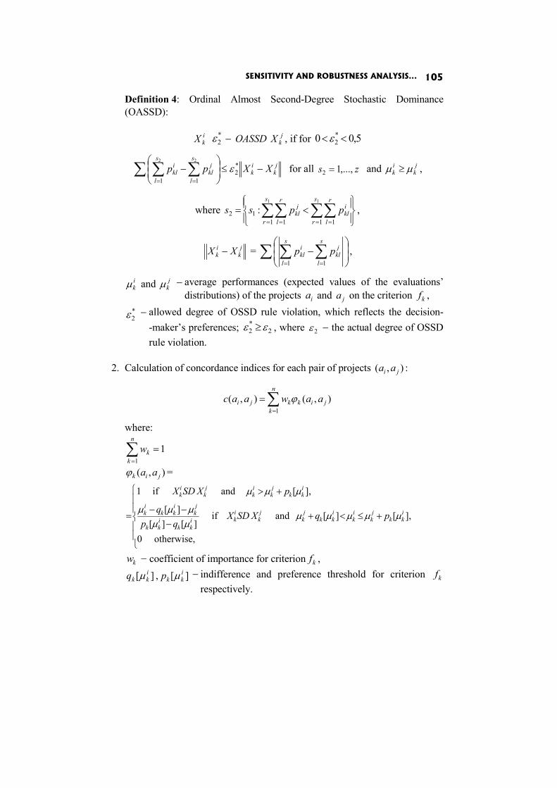
SENSITIVITY AND ROBUSTNESS ANALYSIS... 105
Definition 4: Ordinal Almost Second-Degree Stochastic Dominance (OASSD):
ikX *
2ε − OASSD jkX , if for 5,00 *
2 << ε
jk
ik
s
l
jkl
s
l
ikl XXpp −≤⎟
⎟⎠
⎞⎜⎜⎝
⎛−∑ ∑∑
==
*2
11
22
ε for all zs ,...,12 = and jk
ik μμ ≥ ,
where ⎪⎭
⎪⎬⎫
⎪⎩
⎪⎨⎧
<= ∑∑∑∑= == =
11
1 11 112 :
s
r
r
l
ikl
s
r
r
l
jkl ppss ,
jk
ik XX − = ∑ ∑∑ ⎟
⎟⎠
⎞⎜⎜⎝
⎛−
==
s
l
jkl
s
l
ikl pp
11
,
ikμ and j
kμ − average performances (expected values of the evaluations’distributions) of the projects ia and ja on the criterion kf ,
*2ε − allowed degree of OSSD rule violation, which reflects the decision-
-maker’s preferences; 2*2 εε ≥ , where 2ε − the actual degree of OSSD
rule violation.
2. Calculation of concordance indices for each pair of projects :),( ji aa
),(),(1
ji
n
kkkji aawaac ∑
=
= ϕ
where:
11
=∑=
n
kkw
),( jik aaϕ =
⎪⎪
⎩
⎪⎪
⎨
⎧
+≤<+−
−−
+>
=
otherwise,0
],[][andif][][
][
],[andif1
ikk
jk
ik
ikk
jk
jk
iki
kkikk
jk
ikk
ik
ikk
jk
ik
jk
ik
pqXSDXqp
q
pXSDX
μμμμμμμμμμ
μμμ
kw − coefficient of importance for criterion kf ,
][ ikkq μ , ][ i
kkp μ − indifference and preference threshold for criterion kfrespectively.
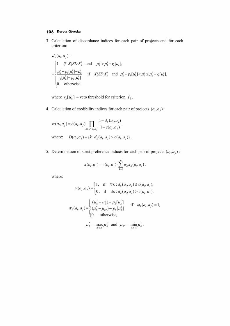
Dorota Górecka 106
3. Calculation of discordance indices for each pair of projects and for each criterion:
),( jik aad =
⎪⎪
⎩
⎪⎪
⎨
⎧
+≤<+−
−−
+>
=
otherwise,0
],[][andif][][
][
],[and1
ikk
ik
jk
ikk
ik
ik
jki
kkikk
ik
ikk
jk
ikk
ik
jk
ik
jk
vpXSDXpv
p
vXSDXif
μμμμμμμ
μμμ
μμμ
where ][ ikkv μ – veto threshold for criterion kf .
4. Calculation of credibility indices for each pair of projects :),( ji aa
∏∈ −
−=
),( ),(1),(1
),(),(ji aaDk ji
jikjiji aac
aadaacaaσ
where: )},(),(:{),( jijikji aacaadkaaD >= .
5. Determination of strict preference indices for each pair of projects ),( ji aa :
∑=
⋅=n
kjikkjiji aawaaaa
1
),(),(),( πνπ ,
where:
⎪⎩
⎪⎨⎧
>∃
≤∀=
),,(),(:if,0
),,(),(:if,1),(
jijik
jijikji aacaadk
aacaadkaaν
⎪⎩
⎪⎨
⎧=
−−−−
=
,otherwise0
,1),(if][)(][)(
),( ** jiki
kkkk
ikk
jk
ik
jikaa
pp
aaϕ
μμμμμμ
π
ikAak
i
μμ∈
= max* and ikAak
i
μμ∈
= min* .
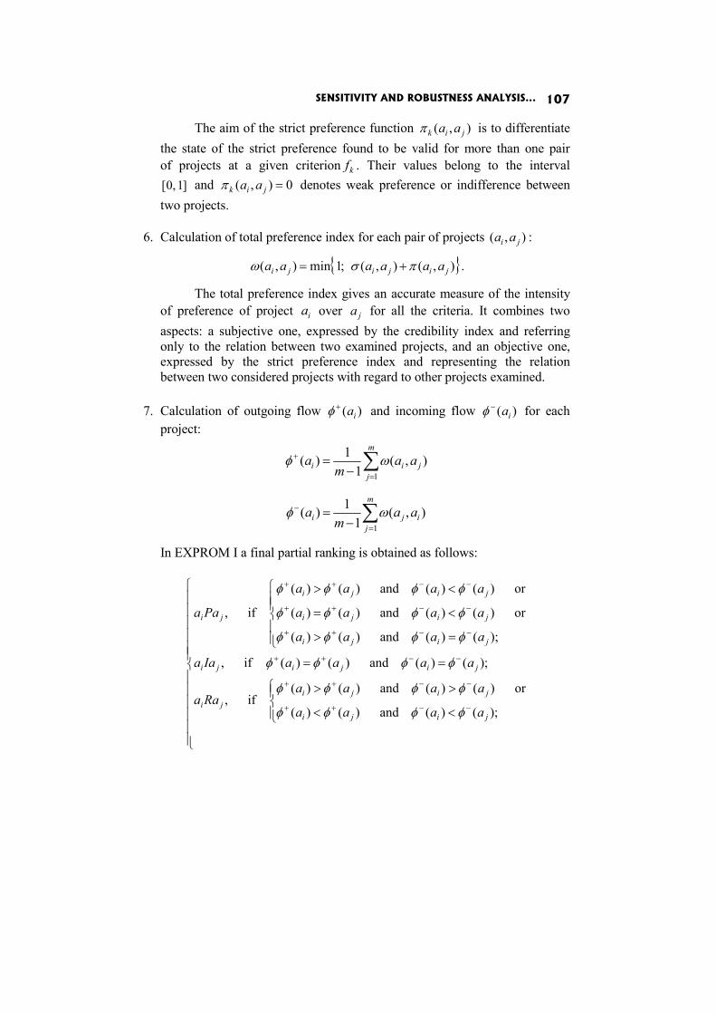
SENSITIVITY AND ROBUSTNESS ANALYSIS... 107
The aim of the strict preference function ),( jik aaπ is to differentiate the state of the strict preference found to be valid for more than one pair of projects at a given criterion kf . Their values belong to the interval
]1,0[ and 0),( =jik aaπ denotes weak preference or indifference between two projects.
6. Calculation of total preference index for each pair of projects ),( ji aa :
{ }),(),(;1min),( jijiji aaaaaa πσω += .
The total preference index gives an accurate measure of the intensity of preference of project ia over ja for all the criteria. It combines two aspects: a subjective one, expressed by the credibility index and referring only to the relation between two examined projects, and an objective one, expressed by the strict preference index and representing the relation between two considered projects with regard to other projects examined.
7. Calculation of outgoing flow )( ia+φ and incoming flow )( ia−φ for each project:
∑=
+
−=
m
jjii aa
ma
1
),(1
1)( ωφ
∑=
−
−=
m
jiji aa
ma
1
),(1
1)( ωφ
In EXPROM I a final partial ranking is obtained as follows:
⎪⎪⎪⎪⎪⎪
⎩
⎪⎪⎪⎪⎪⎪
⎨
⎧
⎪⎩
⎪⎨⎧
<<
>>
==
⎪⎪⎩
⎪⎪⎨
⎧
=>
<=
<>
−−++
−−++
−−++
−−++
−−++
−−++
);()(and)()(
or)()(and)()(if,
);()(and)()(if,
);()(and)()(
or)()(and)()(
or)()(and)()(
if,
jiji
jijiji
jijiji
jiji
jiji
jiji
ji
aaaa
aaaaRaa
aaaaIaa
aaaa
aaaa
aaaa
Paa
φφφφ
φφφφ
φφφφ
φφφφ
φφφφ
φφφφ

Dorota Górecka 108
where P , I and R stand for preference, indifference and incomparability, respectively.
In EXPROM II a final complete ranking is constructed according
to the descending order of the net flows ),( iaφ where ).()()( iii aaa −+ −= φφφ
Appendix B
APPLICATION OF THE EVAMIX METHOD WITH STOCHASTIC
DOMINANCE RULES TO THE EUROPEAN PROJECTS’ SELECTION
In EVAMIX method, proposed by H. Voogd, the qualitative and quantita-tive data are distinguished and the final appraisal score of a given variant is the result of a combination of the evaluations calculated separately for the qualitative and quantitative criteria.
After introducing stochastic dominance rules to EVAMIX method the procedure of ordering projects consists of the following steps:
1. Determination of the qualitative dominance measures for the ordinal criteria:
( ){ } ...,5,3,1 ,)()(sgn
1
=⎥⎥⎦
⎤
⎢⎢⎣
⎡−= ∑
∈
caawc
Ok
c
jkikkij μμα
where:
c − an arbitrary scaling parameter, for which any positive odd value may bechosen; the higher the value of the parameter, the weaker the influenceof the deviations between the evaluations for the less important criteria;
O − a set of qualitative (ordinal) criteria16;
( )⎪⎪⎩
⎪⎪⎨
⎧
>−
>
=−
otherwise, 0
),()( and if 1
),()( and X if 1
)()(sgn ikjkik
jk
jkikj
kik
jkik aaXSDX
aaXSD
aa μμ
μμ
μμ
16 It is assumed that all the criteria are maximized.
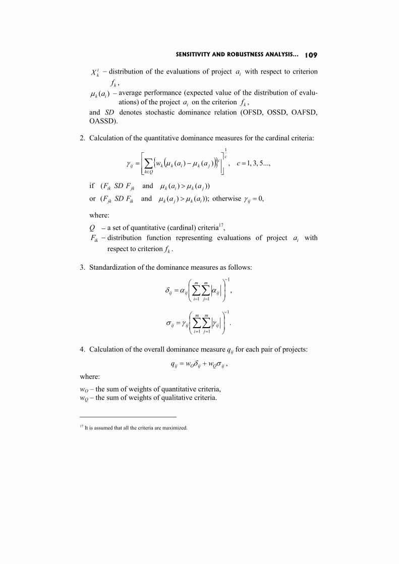
SENSITIVITY AND ROBUSTNESS ANALYSIS... 109
ikX − distribution of the evaluations of project ia with respect to criterion
kf , )( ik aμ − average performance (expected value of the distribution of evalu-
ations) of the project ia on the criterion kf , and SD denotes stochastic dominance relation (OFSD, OSSD, OAFSD, OASSD).
2. Calculation of the quantitative dominance measures for the cardinal criteria:
( ){ } ...,5,3,1 ,)()(
1
=⎥⎥⎦
⎤
⎢⎢⎣
⎡−= ∑
∈
caawc
Qk
cjkikkij μμγ
if ))()(and( jkikjkik aaFSDF μμ >
or ));()(and( ikjkikjk aaFSDF μμ > otherwise ,0=ijγ
where:
Q − a set of quantitative (cardinal) criteria17, ikF − distribution function representing evaluations of project ia with
respect to criterion kf . 3. Standardization of the dominance measures as follows:
,1
1 1
−
= =⎟⎟⎠
⎞⎜⎜⎝
⎛= ∑∑
m
i
m
jijijij ααδ
.1
1 1
−
= =⎟⎟⎠
⎞⎜⎜⎝
⎛= ∑∑
m
i
m
jijijij γγσ
4. Calculation of the overall dominance measure qij for each pair of projects:
ijQijOij wwq σδ += ,
where:
wO – the sum of weights of quantitative criteria, wQ – the sum of weights of qualitative criteria.
17 It is assumed that all the criteria are maximized.
Dorota Górecka 110
5. Determination of the final appraisal score ui for each project as follows:
∑=
=m
jiji q
mu
1
1.
6. Ranking projects according to the descending order of the final appraisal
scores.
References
Brans J.P., Vincke Ph. (1985), A Preference Ranking Organization Method: The PROMETHEE Method for Multiple Criteria Decision-Making, “Management Science”, No. 31.
Brans J.P., Vincke Ph., Mareschal B. (1986), How to Select and How to Rank Projects: The PROMETHEE Method, “European Journal of Operational Research”, No. 24.
Diakoulaki D., Koumoutsos N. (1991), Cardinal Ranking of Alternative Actions: Extension of the PROMETHEE Method, “European Journal of Operational Research”, No. 53.
Dias L.C., Climaco J.N. (1999), On Computing ELECTRE’s Credibility Indices under Partial Information, “Journal of Multi-Criteria Decision Analysis”, No. 8.
Figueira J., Mousseau V., Roy B. (2005), ELECTRE Methods, [in:] Multiple Criteria Decision Analysis: State of the Art Surveys, eds. J. Figueira, S. Greco, M. Ehrgott, Springer, New York.
Figueira J., Roy B. (2002), Determining the Weights of Criteria in the ELECTRE Type Methods with a Revised Simos’ Procedure, “European Journal of Operational Research”, No. 139.
Górecka D. (2009), Wielokryterialne wspomaganie wyboru projektów europejskich, TNOiK „Dom Organizatora”, Toruń.
Górecka D. (2010), Zastosowanie metod wielokryterialnych opartych na relacji przewyższania do oceny europejskich projektów inwestycyjnych, [in:] Metody i zastosowania badań operacyjnych’10, ed. M. Nowak, Wydawnictwo Uni-wersytetu Ekonomicznego, Katowice.
Górecka D. (2011a), Analiza wrażliwości i odporności rozwiązań w procesie selekcji projektów europejskich, [w:] Optymalizacja, klasyfikacja, logistyka. Przykłady zastosowań, red. J.B. Gajda, R. Jadczak, Wydawnictwo Uniwersytetu Łódzkie-go, Łódź.
Górecka D. (2011b), On the Choice of Method in Multi-criteria Decision Aiding Process Concerning European Projects, [in:] Multiple Criteria Decision Making’10-11, eds. T. Trzaskalik, T. Wachowicz, Publisher of The University of Economics in Katowice, Katowice.
SENSITIVITY AND ROBUSTNESS ANALYSIS... 111
Górecka D., Pietrzak M.B. (2012), Zastosowanie metody PROMETHEE II w procesie rankingowania projektów europejskich w ramach Regionalnego Programu Operacyjnego Województwa Kujawsko-Pomorskiego na lata 2007-2013, [w:] Modelowanie preferencji a ryzyko’12, red. T. Trzaskalik, Wydawnictwo Uniwersytetu Ekonomicznego, Katowice.
Hyde K.M., Maier H.R., Colby C.B. (2005), A Distance-based Uncertainty Analysis Approach to Multi-criteria Decision Analysis for Water Resource Decision- -making, “Journal of Environmental Management”, No. 77.
Kahneman D., Tversky A. (1979), Prospect Theory: An Analysis of Decision under Risk, “Econometrica”, No. 47.
Konarzewska-Gubała E. (1991), Wspomaganie decyzji wielokryterialnych: system BIPOLAR, Wydawnictwo Uczelniane Akademii Ekonomicznej, Wrocław.
Leshno M., Levy H. (2002), Preferred by “All” and Preferred by “Most” Decision Makers: Almost Stochastic Dominance, “Management Science”, No. 48.
Lootsma F.A., Mensch T.C.A., Vos F.A. (1990), Multi-criteria Analysis and Budget Reallocation in Long-term Research Planning, “European Journal of Operational Research”, No. 47.
Nowak M. (2005), Investments Projects Evaluation by Simulation and Multiple Criteria Decision Aiding Procedure, „Journal of Civil Engineering and Management”, No. 11.
Olson D.L., G. Fliedner, K. Currie (1995), Comparison of the REMBRANDT system with Analytic Hierarchy Process, “European Journal of Operational Research”, No. 82.
Roubens M. (1982), Preference Relations on Actions and Criteria in Multicriteria Decision Making, „European Journal of Operational Research”, No. 10.
Roy B. (1998), A Missing Link in Operational Research – Decision Aiding: Robustness Analysis, “Foundations of Computing and Decision Sciences”, No. 23.
Roy B., J. Hugonnard (1982), Ranking of Suburban Line Extension Projects on the Paris Metro System by a Multi-criteria Method, „Transportation Research”, No. 16A.
Saaty T.L. (2006), Fundamentals of Decision Making and Priority Theory with the Analytic Hierarchy Process, Vol. VI of the AHP Series, RWS Publications, Pittsburgh.
Saaty T.L., Vargas L.G. (1991), The Logic of Priorities. Applications of the Analytic Hierarchy Process in Business, Energy, Health & Transportation, Vol. III of the AHP Series, RWS Publications, Pittsburgh.
Spector Y., Leshno M., Ben Horin M. (1996), Stochastic Dominance in an Ordinal World, „European Journal of Operational Research”, No. 93.
Voogd H. (1982), Multicriteria Evaluation with Mixed Qualitative and Quantitative Data, “Environment and Planning B”, No. 9.
Josef Jablonsky
MULTICRITERIA ANALYSIS OF CLASSIFICATION IN ATHLETIC DECATHLON
Abstract
Man’s decathlon is an athletic contest which consists of 10 events, four of them measured in seconds and the remaining six in meters. Each athlete (alternative) is described by his 10 results (criteria). Current system of classification is based on aggregation of results using utility (scoring) functions which are defined exactly for each event. This system has been used since 1984 and the aim of the paper is to analyse it with respect to current conditions. The current method of classification is compared with several alternative methods which better reflect current top results of 10 events included in men decathlon. Proposed methods are applied to real results, specifically to the Olympic Games 2008.
Keywords
Multiple criteria decision making, decathlon, utility function.
Introduction
Decathlon is an athletic contest with a very long tradition which consists of 10 different events. Since ancient Greece it has been regarded as a measure of universality of athletes and is often called „king athletic event”. For the first time a kind of athletic multicontest was scheduled in the 3rd Summer Olympic Games in Saint Louis in 1904. In 1914 the decathlon was established by the International Amateur Athletic Federation in the form in which it is known now. Since that year the decathlon consists of 10 events (3 sprints, 1 long distance run, 3 jump events and 3 throw events) and the order of all events within a contest is fixed. The contest is always scheduled in two consecutive days as follows: 1st day: – 100 meters run, – Long jump, – Shot put,
MULTICRITERIA ANALYSIS OF CLASSIFICATION… 113
– High jump, – 400 meters run, 2nd day: – 110 meters hurdles run, – Discus throw, – Pole vault, – Javelin throw, – 1500 meters run. Principles of decathlon, its history and the current system of scoring are described in detail in an official IAAF paper [Diack 2004].
In general, ranking of contestants in decathlon is a multiple criteria decision problem (MCDM) with athletes attending the contest as alternatives and 10 criteria. The aim of the problem is to evaluate the alternatives (athletes) and rank them from the best to the worst. As it is clear, criterion values in this problem are not comparable – they are given either in seconds or in centimeters and moreover the values in seconds (centimeters) are incomparable directly. That is why the results of athletes in individual events are aggregated using so-called scoring tables which assign points to the performances in individual events. The athletes are ranked according to the total points achieved.
1. Current system of performance evaluation in decathlon
The scoring tables went over time through several evolution steps – [for details see: Diack 2004]. Their last change is dated 1984 and the tables constructed according to the following principles still stand today: 1. The scoring tables should differ from those used for individual event
scoring. 2. The scores for different events should be comparable, so that equal skill
levels in different events are rewarded with equal point levels. 3. The scoring tables should be one of the following:
– linear in all events, or – slightly progressive in all events.
4. The tables should be applicable to all levels of performance, from youth to professional.
5. Men and women should have different tables. 6. Specialists' performances should be the basis for the scores in the tables. 7. The tables should be applicable in the future.
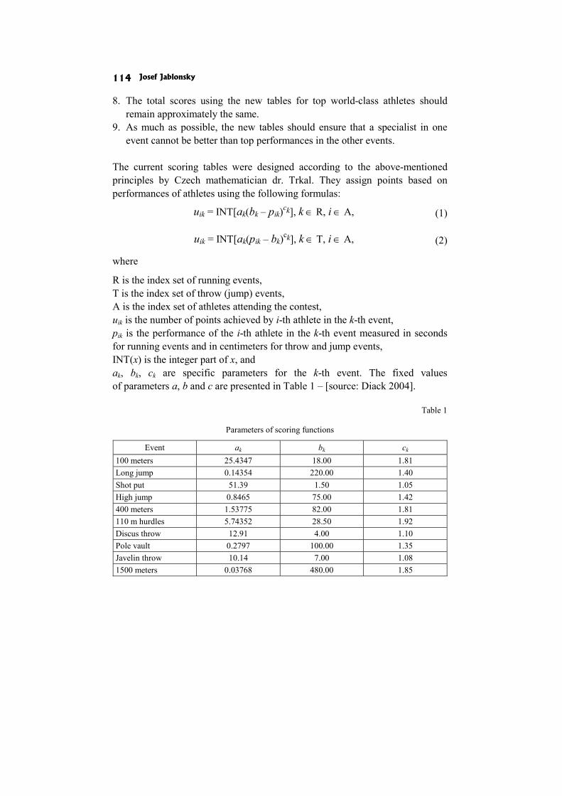
Josef Jablonsky 114
8. The total scores using the new tables for top world-class athletes should remain approximately the same.
9. As much as possible, the new tables should ensure that a specialist in one event cannot be better than top performances in the other events.
The current scoring tables were designed according to the above-mentioned principles by Czech mathematician dr. Trkal. They assign points based on performances of athletes using the following formulas:
uik = INT[ak(bk – pik)ck], k ∈ R, i ∈ A, (1)
uik = INT[ak(pik – bk)ck], k ∈ T, i ∈ A, (2)
where
R is the index set of running events, T is the index set of throw (jump) events, A is the index set of athletes attending the contest, uik is the number of points achieved by i-th athlete in the k-th event, pik is the performance of the i-th athlete in the k-th event measured in seconds for running events and in centimeters for throw and jump events, INT(x) is the integer part of x, and ak, bk, ck are specific parameters for the k-th event. The fixed values of parameters a, b and c are presented in Table 1 – [source: Diack 2004].
Table 1
Parameters of scoring functions
Event ak bk ck 100 meters 25.4347 18.00 1.81 Long jump 0.14354 220.00 1.40 Shot put 51.39 1.50 1.05 High jump 0.8465 75.00 1.42 400 meters 1.53775 82.00 1.81 110 m hurdles 5.74352 28.50 1.92 Discus throw 12.91 4.00 1.10 Pole vault 0.2797 100.00 1.35 Javelin throw 10.14 7.00 1.08 1500 meters 0.03768 480.00 1.85
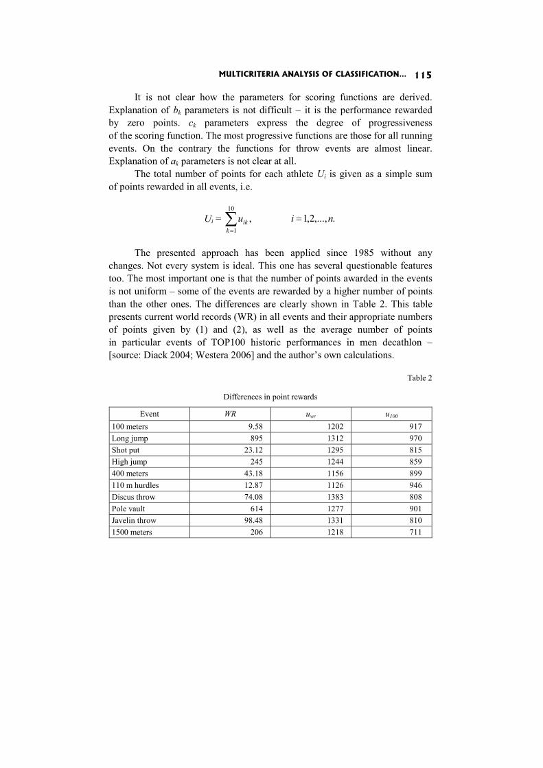
MULTICRITERIA ANALYSIS OF CLASSIFICATION… 115
It is not clear how the parameters for scoring functions are derived. Explanation of bk parameters is not difficult − it is the performance rewarded by zero points. ck parameters express the degree of progressiveness of the scoring function. The most progressive functions are those for all running events. On the contrary the functions for throw events are almost linear. Explanation of ak parameters is not clear at all.
The total number of points for each athlete Ui is given as a simple sum of points rewarded in all events, i.e.
Ui = .,...,2,1,10
1
niuk
ik =∑=
The presented approach has been applied since 1985 without any changes. Not every system is ideal. This one has several questionable features too. The most important one is that the number of points awarded in the events is not uniform – some of the events are rewarded by a higher number of points than the other ones. The differences are clearly shown in Table 2. This table presents current world records (WR) in all events and their appropriate numbers of points given by (1) and (2), as well as the average number of points in particular events of TOP100 historic performances in men decathlon – [source: Diack 2004; Westera 2006] and the author’s own calculations.
Table 2
Differences in point rewards
Event WR uwr u100 100 meters 9.58 1202 917 Long jump 895 1312 970 Shot put 23.12 1295 815 High jump 245 1244 859 400 meters 43.18 1156 899 110 m hurdles 12.87 1126 946 Discus throw 74.08 1383 808 Pole vault 614 1277 901 Javelin throw 98.48 1331 810 1500 meters 206 1218 711
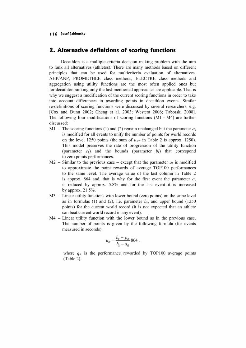
Josef Jablonsky 116
2. Alternative definitions of scoring functions
Decathlon is a multiple criteria decision making problem with the aim to rank all alternatives (athletes). There are many methods based on different principles that can be used for multicriteria evaluation of alternatives. AHP/ANP, PROMETHEE class methods, ELECTRE class methods and aggregation using utility functions are the most often applied ones but for decathlon ranking only the last-mentioned approaches are applicable. That is why we suggest a modification of the current scoring functions in order to take into account differences in awarding points in decathlon events. Similar re-definitions of scoring functions were discussed by several researchers, e.g. [Cox and Dunn 2002; Cheng et al. 2003; Westera 2006; Taborski 2008]. The following four modifications of scoring functions (M1 – M4) are further discussed: M1 − The scoring functions (1) and (2) remain unchanged but the parameter ak
is modified for all events to unify the number of points for world recordson the level 1250 points (the sum of uWR in Table 2 is approx. 1250).This model preserves the rate of progression of the utility function(parameter ck) and the bounds (parameter bk) that correspondto zero points performances.
M2 − Similar to the previous case – except that the parameter ak is modifiedto approximate the point rewards of average TOP100 performancesto the same level. The average value of the last column in Table 2is approx. 864 and, that is why for the first event the parameter ak
is reduced by approx. 5.8% and for the last event it is increasedby approx. 21.5%.
M3 − Linear utility functions with lower bound (zero points) on the same levelas in formulas (1) and (2), i.e. parameter bk, and upper bound (1250points) for the current world record (it is not expected that an athletecan beat current world record in any event).
M4 − Linear utility function with the lower bound as in the previous case.The number of points is given by the following formula (for eventsmeasured in seconds):
864ikk
ikkik qb
pbu−−
= ,
where qik is the performance rewarded by TOP100 average points(Table 2).
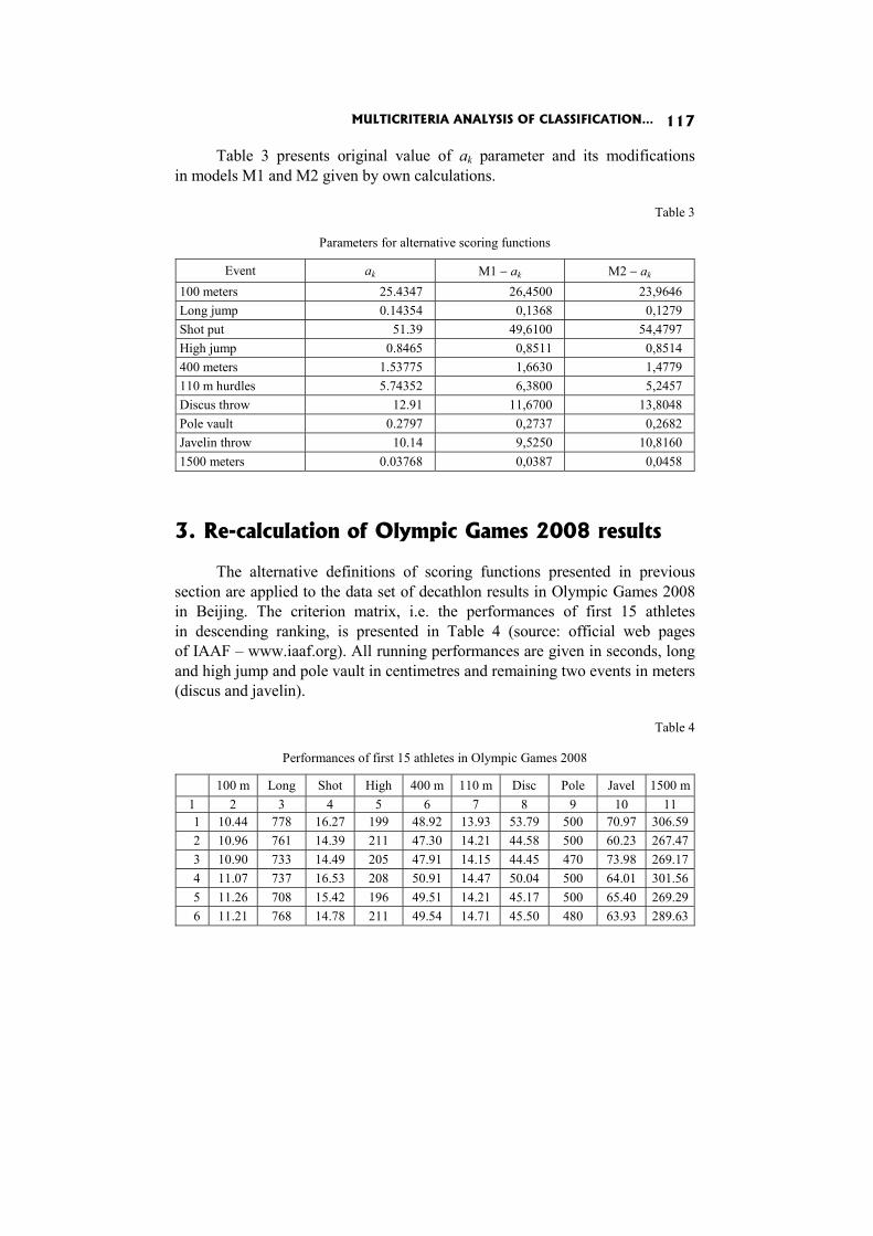
MULTICRITERIA ANALYSIS OF CLASSIFICATION… 117
Table 3 presents original value of ak parameter and its modifications in models M1 and M2 given by own calculations.
Table 3
Parameters for alternative scoring functions
Event ak M1 − ak M2 − ak 100 meters 25.4347 26,4500 23,9646 Long jump 0.14354 0,1368 0,1279 Shot put 51.39 49,6100 54,4797 High jump 0.8465 0,8511 0,8514 400 meters 1.53775 1,6630 1,4779 110 m hurdles 5.74352 6,3800 5,2457 Discus throw 12.91 11,6700 13,8048 Pole vault 0.2797 0,2737 0,2682 Javelin throw 10.14 9,5250 10,8160 1500 meters 0.03768 0,0387 0,0458
3. Re-calculation of Olympic Games 2008 results
The alternative definitions of scoring functions presented in previous section are applied to the data set of decathlon results in Olympic Games 2008 in Beijing. The criterion matrix, i.e. the performances of first 15 athletes in descending ranking, is presented in Table 4 (source: official web pages of IAAF – www.iaaf.org). All running performances are given in seconds, long and high jump and pole vault in centimetres and remaining two events in meters (discus and javelin).
Table 4
Performances of first 15 athletes in Olympic Games 2008
100 m Long Shot High 400 m 110 m Disc Pole Javel 1500 m 1 2 3 4 5 6 7 8 9 10 11 1 10.44 778 16.27 199 48.92 13.93 53.79 500 70.97 306.59 2 10.96 761 14.39 211 47.30 14.21 44.58 500 60.23 267.47 3 10.90 733 14.49 205 47.91 14.15 44.45 470 73.98 269.17 4 11.07 737 16.53 208 50.91 14.47 50.04 500 64.01 301.56 5 11.26 708 15.42 196 49.51 14.21 45.17 500 65.40 269.29 6 11.21 768 14.78 211 49.54 14.71 45.50 480 63.93 289.63
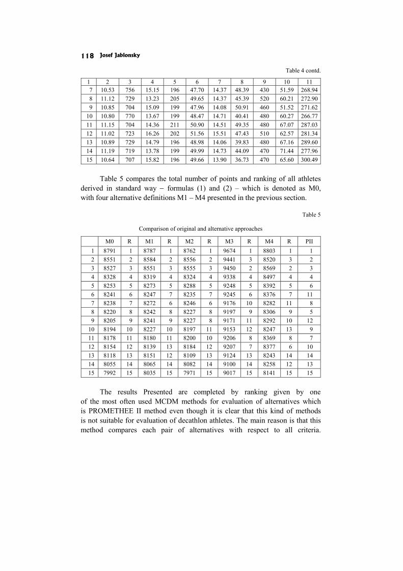
Josef Jablonsky 118
Table 4 contd.
1 2 3 4 5 6 7 8 9 10 11 7 10.53 756 15.15 196 47.70 14.37 48.39 430 51.59 268.94 8 11.12 729 13.23 205 49.65 14.37 45.39 520 60.21 272.90 9 10.85 704 15.09 199 47.96 14.08 50.91 460 51.52 271.62
10 10.80 770 13.67 199 48.47 14.71 40.41 480 60.27 266.77 11 11.15 704 14.36 211 50.90 14.51 49.35 480 67.07 287.03 12 11.02 723 16.26 202 51.56 15.51 47.43 510 62.57 281.34 13 10.89 729 14.79 196 48.98 14.06 39.83 480 67.16 289.60 14 11.19 719 13.78 199 49.99 14.73 44.09 470 71.44 277.96 15 10.64 707 15.82 196 49.66 13.90 36.73 470 65.60 300.49
Table 5 compares the total number of points and ranking of all athletes
derived in standard way − formulas (1) and (2) – which is denoted as M0, with four alternative definitions M1 – M4 presented in the previous section.
Table 5
Comparison of original and alternative approaches
M0 R M1 R M2 R M3 R M4 R PII 1 8791 1 8787 1 8762 1 9674 1 8803 1 1 2 8551 2 8584 2 8556 2 9441 3 8520 3 2 3 8527 3 8551 3 8555 3 9450 2 8569 2 3 4 8328 4 8319 4 8324 4 9338 4 8497 4 4 5 8253 5 8273 5 8288 5 9248 5 8392 5 6 6 8241 6 8247 7 8235 7 9245 6 8376 7 11 7 8238 7 8272 6 8246 6 9176 10 8282 11 8 8 8220 8 8242 8 8227 8 9197 9 8306 9 5 9 8205 9 8241 9 8227 8 9171 11 8292 10 12
10 8194 10 8227 10 8197 11 9153 12 8247 13 9 11 8178 11 8180 11 8200 10 9206 8 8369 8 7 12 8154 12 8139 13 8184 12 9207 7 8377 6 10 13 8118 13 8151 12 8109 13 9124 13 8243 14 14 14 8055 14 8065 14 8082 14 9100 14 8258 12 13 15 7992 15 8035 15 7971 15 9017 15 8141 15 15
The results Presented are completed by ranking given by one
of the most often used MCDM methods for evaluation of alternatives which is PROMETHEE II method even though it is clear that this kind of methods is not suitable for evaluation of decathlon athletes. The main reason is that this method compares each pair of alternatives with respect to all criteria.
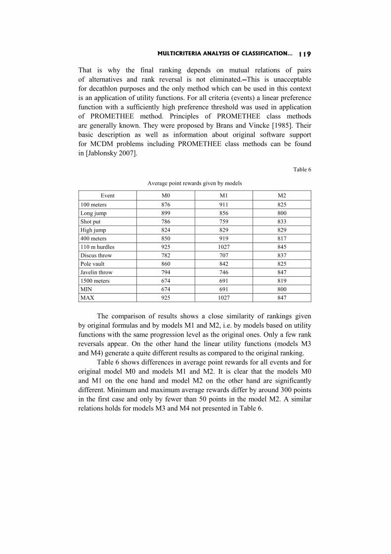
MULTICRITERIA ANALYSIS OF CLASSIFICATION… 119
That is why the final ranking depends on mutual relations of pairs of alternatives and rank reversal is not eliminated. This is unacceptable for decathlon purposes and the only method which can be used in this context is an application of utility functions. For all criteria (events) a linear preference function with a sufficiently high preference threshold was used in application of PROMETHEE method. Principles of PROMETHEE class methods are generally known. They were proposed by Brans and Vincke [1985]. Their basic description as well as information about original software support for MCDM problems including PROMETHEE class methods can be found in [Jablonsky 2007].
Table 6
Average point rewards given by models
Event M0 M1 M2 100 meters 876 911 825 Long jump 899 856 800 Shot put 786 759 833 High jump 824 829 829 400 meters 850 919 817 110 m hurdles 925 1027 845 Discus throw 782 707 837 Pole vault 860 842 825 Javelin throw 794 746 847 1500 meters 674 691 819 MIN 674 691 800 MAX 925 1027 847
The comparison of results shows a close similarity of rankings given
by original formulas and by models M1 and M2, i.e. by models based on utility functions with the same progression level as the original ones. Only a few rank reversals appear. On the other hand the linear utility functions (models M3 and M4) generate a quite different results as compared to the original ranking.
Table 6 shows differences in average point rewards for all events and for original model M0 and models M1 and M2. It is clear that the models M0 and M1 on the one hand and model M2 on the other hand are significantly different. Minimum and maximum average rewards differ by around 300 points in the first case and only by fewer than 50 points in the model M2. A similar relations holds for models M3 and M4 not presented in Table 6.
Josef Jablonsky 120
Conclusions
Analysis of decathlon results is a very interesting multiple criteria decision making problem of high importance. The paper presents current system of evaluation based on aggregation of performances in events into final point score and proposes several new definitions of scoring functions. The most promising definition has been introduced as model M2. It solves the problem of high differences in point rewards and preserves the current level of progression in individual events. Moreover, results of the model M2 keep the current final level of points and seem to be comparable to the current standard system.
Acknowledgements
The research is supported by the Grant Agency of the Czech Republic − project no. 402/12/1387, and by IGA project F4/18/2011.
References
Brans J.P., Vincke, P. (1985), A Preference Ranking Organisation Method (The PROMETHEE Method for Multiple Criteria Decision-Making), “Management Science”, No. 31(6).
Cheng C.L, Tsai C.H., Chen L. (2003), Applying Grey Relational Analysis to the Decathlon Evaluation Model, “International Journal of The Computer, “The Internet and Management”, No. 11(3).
Cox D.F, Dunn R.T. (2002), An Analysis of Decathlon Data, “The Statistician”, No. 52(2).
Diack L. (2004), IAAF Scoring Tables for Conbined Events – accessible at http:// www.iaaf.org/mm/Document/Competitions/TechnicalArea/ ScoringTables_CE_ 744.pdf [08.03.2011].
Jablonsky J. (2007), Optimisation and Modelling with Spreadsheets, in: Proceedings of the SOR'07, BORI, Ljubljana.
Taborski J. (2008), Quantitative Methods in Athletic Decathlon (in Czech), VSE Praha. Westera W. (2006), Decathlon, Towards a Balanced and Sustainable Performance
Assessment Method, “New Studies in Athletics”, March/April, pp. 37-48 − accessible at http://www.open.ou.nl/wim/publicationspdf/ [08.03.2011].
Ignacy Kaliszewski
Janusz Miroforidis
REAL AND VIRTUAL PARETO SET UPPER APPROXIMATIONS
Abstract
This paper deals with the problem of the derivation of lower and upper approximations of an efficient element set.
We consider the case where upper approximations cannot be derived as criteria mapping images of infeasible variants.
Keywords
Multiobjective optimization, evolutionary algorithms, lower Pareto set approximations, upper Pareto set approximations.
Introduction
Under assumption that all criteria are of the type “the more the better” each outcome (i.e. the image of an admissible variant under the criteria mapping) lies “below” the Pareto set (the set of efficient outcomes) or is an element of this set. A number of such outcomes form a lower approximation of the Pareto set.
By analogy, we consider an upper approximation of the Pareto set, i.e. a set of elements of the outcome (criteria) space which lie “above” the Pareto set.
Having pairs of lower and upper approximations is of interest for two reasons. First, provided that elements of a lower and upper approximation are uniformly distributed along the Pareto set, we are in position to assess the maximal error one makes when representing an efficient outcome y by an outcome y’ taken from the lower approximation and dominated by y [Kaliszewski 2008; Miroforidis 2008, 2010; Kaliszewski et al. 2011, 2012]. That is important in cases where deriving elements of the Pareto set is com-putationally costly and working with lower approximations of the Pareto set
Ignacy Kaliszewski, Janusz Miroforidis 122
instead of the Pareto set itself is a rational option. Second, given a pair of lower and upper approximations lower and upper bounds on components of any efficient outcome pointed to by the Decision Maker preferences can be easily calculated. How the Decision Maker preferences point to efficient outcomes will be explained below.
In this paper we discuss problems arising when deriving upper approximations and we illustrate our considerations by an illustrative example.
In our earlier papers we have proposed to conduct interactive multiple criteria decision processes with outcome assessments instead of outcomes themselves [Miroforidis 2008, 2010; Kaliszewski, Miroforidis 2010a, b; Kaliszewski et al. 2011]. By an outcome assessment we mean lower and upper bounds on values of outcome components. Such an approach stemmed from a variety of Multiple Criteria Decision Making problems where efficient out-comes are given implicitly by a set of constraints and therefore have to be derived by solving optimization problems. To provide for versatility of such an approach we have adapted it to employ evolutionary calculations (Evolutio-nary Multiobjective Optimization) driven by Decision Maker preferences revealed in the course of interactive decision processes.
We have founded our approach on two constructs, namely on lower approximations, i.e. finite subsets of feasible variants, and upper approxi-mations, i.e. finite subsets of infeasible variants with some specific properties. The formal definitions of both constructs are given in the next section.
Of interest are lower and upper approximations which are tight, i.e. their images under the criteria mapping are close, in a sense, to the set of efficient outcomes. Tight approximations provide for tight bounds in outcome assess-ments mentioned above. Moreover, images of tight lower and upper approxi-mations represent sets of efficient outcomes within measurable accuracy. Except for our earlier papers we are aware of only one paper attempting to exploit a similar concept, namely Legriel et al. [2010].
Evolutionary Multiobjective Optimization (EMO) methods and algorithms are dedicated to deriving tight lower approximations and that subject is represented by numerous publications, see e.g. Deb [2001], Coello Coello et al. [2002]. In contrast to this, deriving lower and upper approximations is a novel concept.
A lower approximation always exists as long as the set of feasible variants is nonempty. However, the existence of an upper approximation is not guaranteed in general. In this work we consider the case where upper approximations cannot be derived as images of infeasible variants under criteria mappings.
REAL AND VIRTUAL PARETO SET UPPER APPROXIMATIONS 123
The outline of the paper is as follows. In Section 1 we provide basic definitions and notation. In Section 2 we briefly outline the concept of approximating the set of efficient outcomes with the help of lower shells and upper shells. In Section 3 we address the case where upper shells do not exist and propose how to deal with that case to have our concept of outcome assessments still workable. Section 4 concludes.
1. Definitions and notation
Let x denote a (decision) variant, X a space of variants, 0X a set of feasible variants, .0 XX ⊆ Here we assume that X and 0X are infinite. Then the underlying model for MCDM is formulated as:
“max” f (x)
0Xx∈ , (1)
where kRXf →: , ),...,( 1 kfff = , kiRXfi ,...,1,: =→ , ,2≥k are criteria functions; ”max” denotes the operator of deriving all efficient variants (as defined below) in 0X .
Element t of ,, kRTT ⊆ is: – efficient in ,T if ii tt ≥ , ,,...,1 ki = ,Tt ∈ implies ,tt = – weakly efficient in ,T if there is no ,Tt ∈ such that ii tt > , .,...,1 ki =
Variant 0Xx ∈ is called efficient (weakly efficient) in 0X if )(xfy = is efficient (weakly efficient) in ).( 0Xf Elements of )( 0Xf are called out-comes.
We denote the set of efficient variants of 0X by .N Elements of )(Nf are called efficient outcomes for, by the definition, they are efficient in ).( 0Xf
We define on X − the dominance relation p ,
)()'(' xfxfxx <<⇔p ,
where << denotes ,,...,1),()'( kixfxf ii =≤ and )()'( xfxf ii < for at least one i . If ,' xx p then we say that 'x is dominated by x and x is dominating '.x
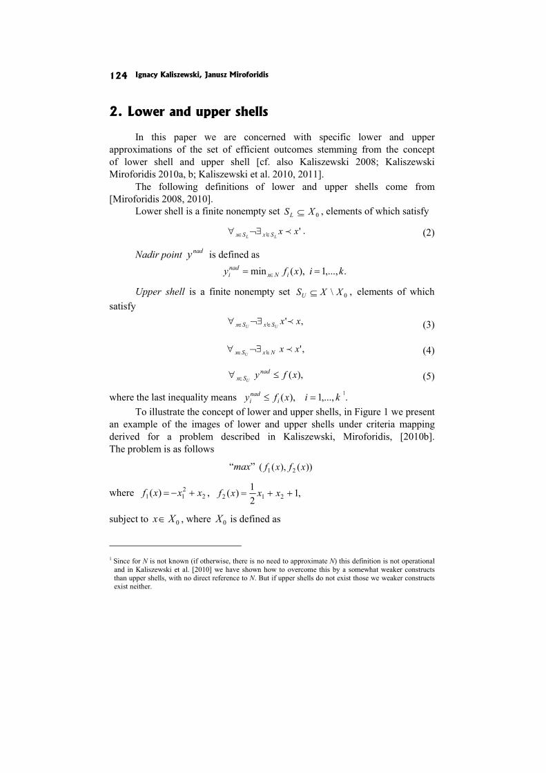
Ignacy Kaliszewski, Janusz Miroforidis 124
2. Lower and upper shells
In this paper we are concerned with specific lower and upper approximations of the set of efficient outcomes stemming from the concept of lower shell and upper shell [cf. also Kaliszewski 2008; Kaliszewski Miroforidis 2010a, b; Kaliszewski et al. 2010, 2011].
The following definitions of lower and upper shells come from [Miroforidis 2008, 2010].
Lower shell is a finite nonempty set 0XSL ⊆ , elements of which satisfy
'' xxLL SxSx p∈∈ ¬∃∀ . (2)
Nadir point nady is defined as .,...,1),(min kixfy iNx
nadi == ∈
Upper shell is a finite nonempty set 0\ XXSU ⊆ , elements of which satisfy
,'' xxUU SxSx p∈∈ ¬∃∀ (3)
,'' xxNxSx Up∈∈ ¬∃∀ (4)
),(xfy nadSx U
≤∀ ∈ (5)
where the last inequality means kixfy inadi ,...,1),( =≤ 1.
To illustrate the concept of lower and upper shells, in Figure 1 we present an example of the images of lower and upper shells under criteria mapping derived for a problem described in Kaliszewski, Miroforidis, [2010b]. The problem is as follows
“max” ))(),(( 21 xfxf
where 2211 )( xxxf +−= , ,1
21)( 212 ++= xxxf
subject to 0Xx ∈ , where 0X is defined as
1 Since for N is not known (if otherwise, there is no need to approximate N) this definition is not operational
and in Kaliszewski et al. [2010] we have shown how to overcome this by a somewhat weaker constructs than upper shells, with no direct reference to N. But if upper shells do not exist those we weaker constructs exist neither.
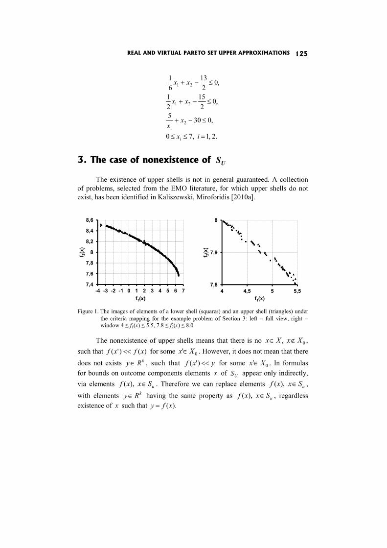
REAL AND VIRTUAL PARETO SET UPPER APPROXIMATIONS 125
.2,1,70
,0305
,02
1521
,02
1361
21
21
21
=≤≤
≤−+
≤−+
≤−+
ix
xx
xx
xx
i
3. The case of nonexistence of US
The existence of upper shells is not in general guaranteed. A collection of problems, selected from the EMO literature, for which upper shells do not exist, has been identified in Kaliszewski, Miroforidis [2010a].
Figure 1. The images of elements of a lower shell (squares) and an upper shell (triangles) under the criteria mapping for the example problem of Section 3: left − full view, right − window 4 ≤ f1(x) ≤ 5.5, 7.8 ≤ f2(x) ≤ 8.0
The nonexistence of upper shells means that there is no 0, XxXx ∉∈ ,
such that )()'( xfxf << for some 0' Xx ∈ . However, it does not mean that there does not exists kRy ∈ , such that yxf <<)'( for some 0' Xx ∈ . In formulas for bounds on outcome components elements x of US appear only indirectly, via elements uSxxf ∈),( . Therefore we can replace elements uSxxf ∈),( , with elements kRy ∈ having the same property as uSxxf ∈),( , regardless existence of x such that ).(xfy =
7,4
7,6
7,8
8
8,2
8,4
8,6
-4 -3 -2 -1 0 1 2 3 4 5 6 7
f 2(x)
f1(x)
7,8
7,9
8
4 4,5 5 5,5
f 2(x)
f1(x)
Ignacy Kaliszewski, Janusz Miroforidis 126
To implement this concept we are to define an appropriate counterpart of the notion upper shell. We shall call such a construct a virtual upper shell.
Virtual upper shell is a finite nonempty set ),(\ 0XfRVS kU ⊆ elements
of which satisfy
,'' yyUU VSyVSy <<¬∃∀ ∈∈ (7)
),(xfyNxVSy U<<¬∃∀ ∈∈ (8)
.yynadVSy U
≤∀ ∈ (9)
In the algorithm presented below we operationalize the condition (8) replacing it by
).(xfyLU SxVSy <<¬∃∀ ∈∈ (8’)
The following EMO-type algorithm derives virtual upper shells. It builds directly on the logic of algorithm PDAE/M proposed in Miroforidis [2010], cf. also Kaliszewski et al. [2011, 2012].
To limit the domain of searching through the set ),(\ 0XfRk we assume existence of bounded set (box)
},,...,1,|{ kiYyYRyR Ui
Li
kkDEC =≤≤∈=
such that ).int()( 0kDECRXf ⊆
Algorithm PDAE/M_VSU
1. 1 == :,0: jLSj Ø, =:j
UVS Ø.
2. Generate randomly 1≥η elements of 0X and derive from those elements 0LS .
3. jLSS =: ; for each element x of S perform Steps 4-6.
4. Select element 0' Xx ∈ such that .' xx p¬ Select element kDECRy ∈'
such that '.)( yxf <<
REAL AND VIRTUAL PARETO SET UPPER APPROXIMATIONS 127
5. If xxSx jL p':∈¬∃ then
5.1. },'{: xSS jL
jL ∪=
5.2. }.'|{\: xxSxSS jL
jL
jL p∈=
6. If ')(:0 yxfXx =∈¬∃ and ': yyVSy jU <<∈¬∃ and
)(': xfySx jL <<∈¬∃ then
6.1. },'{: yVSVS jU
jU ∪=
6.2. }.'|{\: yyVSyVSVS jU
jU
jU <<∈=
7. If maxjj = then STOP, otherwise 1+= jj and go to 3.
Step 1 initializes, whereas in Step 2 an initial lower shell is derived from a number of elements of 0X .
Step 3 specifies that an attempt to modify jLS has to be made at each
of its elements. It has been found in Miroforids [2010] that such a deterministic strategy, as opposed to random selection of elements to be modified, reduces clustering of elements in j
LS and thus produces much more uniform lower approximations of .N
The evolutionary multiobjective optimization principle is realized in Step 4 via the mutation operation. In this step element 'x is selected in the following process:
4.1. xx =:' .
4.2. ).,1( mrndInti =
4.3. If 5.0)1,0( ≤= rndInti then
);)1,0(1)('(':')1(2 maxj
j
iUiii rndxXxx
−
−−+=
otherwise
).)1,0(1)('(':')1(2 maxj
jLiiii rndXxxx
−
−−+=
4.4. If xx p¬' then go to 5; otherwise go to 4.1.
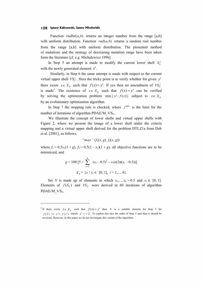
Ignacy Kaliszewski, Janusz Miroforidis 128
Function ),( barndInt returns an integer number from the range [a,b] with uniform distribution. Function ),( barnd returns a random real number from the range [a,b] with uniform distribution. The presented method of mutations and the strategy of decreasing mutation range have been taken form the literature [cf. e.g. Michalewicz 1996].
In Step 5 an attempt is made to modify the current lower shell jLS
with the newly generated element 'x . Similarly, in Step 6 the same attempt is made with respect to the current
virtual upper shell jUVS . Here the tricky point is to verify whether for given 'y
there exists 0Xx ∈ such that '.)( yxf = If yes then no amendment of jUVS
is made2. The existence of 0Xx ∈ such that ')( yxf = can be verified by solving the optimization problem ||)('||min xfy − subject to 0Xx ∈ by an evolutionary optimization algorithm.
In Step 7 the stopping rule is checked, where maxj is the limit for the number of iterations of algorithm PDAE/M_VSU.
We illustrate the concept of lower shells and virtual upper shells with Figure 2, where we present the image of a lower shell under the criteria mapping and a virtual upper shell derived for the problem DTLZ1a from Deb et al. [2001], as follows.
“max” (f1(x, g), f2(x, g))
where f1 = 0.5x1(1 + g), f2 = 0.5(1 – x1)(1 + g), all objective functions are to be minimized, and
g = 100 [5 + ∑=
6
2i
(xi – 0.5)2 − cos(2π(xi – 0.5))]
0X = {x | xi ∈ [0, 1], i = 1,..., 6}.
Set N is made up of elements in which x2,..., x6 = 0.5 and x1 ∈ [0, 1]. Elements of )( LSf and UVS were derived in 60 iterations of algorithm PDAE/M_VSU.
2 If there exists 0Xx ∈ such that ')( yxf = then x is a suitable element for Step 5 for
)'(')( xfyxf =<< entails xx p¬' . To exploit this fact the order of Step 5 and Step 6 should be reversed. However, in this paper we do not investigate this variant of the algorithm.
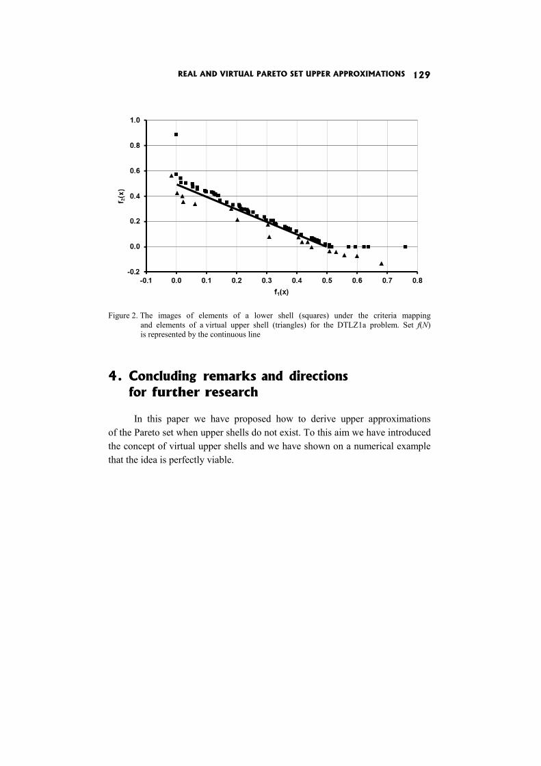
REAL AND VIRTUAL PARETO SET UPPER APPROXIMATIONS 129
Figure 3 shows the criteria mapping of 200 feasible (squares)
and infeasible (triangles) variants generated randomly for the problem DTLZ1a. Variants have been generated from a box containing 0X and checked
for feasibility. As expected, no elements of kR dominating any element of )(Nf have been produced. It can be proved that no such element exists.
Figure 2. The images of elements of a lower shell (squares) under the criteria mapping
and elements of a virtual upper shell (triangles) for the DTLZ1a problem. Set f(N) is represented by the continuous line
4. Concluding remarks and directions for further research
In this paper we have proposed how to derive upper approximations of the Pareto set when upper shells do not exist. To this aim we have introduced the concept of virtual upper shells and we have shown on a numerical example that the idea is perfectly viable.
Ignacy Kaliszewski, Janusz Miroforidis 130
Figure 3. The images of feasible variants (squares) and infeasible variants (triangles) of total 200
variants generated randomly under the criteria mapping for the DTLZ1a problem. Set f(N) is represented by the continuous line
With virtual upper shells in place we are in the position to derive, for any
instance of problem (1), an approximation of the Pareto set in the form of a pair of a lower approximation ),( LSf where LS is a lower shell, and an upper approximation in the form of UVS .
In our previous papers we addressed the problem of efficiency of algorithms we proposed to derive US . The question of efficiency of the algorithm we proposed in this work to derive UVS has been left to further research.
References
Coello Coello C.A., Van Veldhuizen D.A., Lamont G.B. (2002), Evolutionary Algorithms for Solving Multi-Objective Problems, Kluwer Academic Publishers, New York.
Deb K. (2001), Multi-objective Optimization Using Evolutionary Algorithms, John Wiley and Sons, Chichester.
Deb K., Thiele L., Laumanns M., Zitzler E. (2001), Scalable Test Problems for Evolutionary Multi-objective Optimization, TIK-Technical Report No. 112, Institut für Technische Informatik und Kommunikationsnetze, ETH Zürich.

REAL AND VIRTUAL PARETO SET UPPER APPROXIMATIONS 131
Kaliszewski I. (2008), Multiple Criteria Decision Making: Outcome Assessments with Lower and Upper Shells, Systems Research Institute Report RB/9/2008, Warszawa.
Kaliszewski I., Miroforidis J. (2010), Engineering Inspired Test Problems for “Inter-active Multiple Criteria Decision Making Based on Preference Driven Evolutio-nary Multiobjective Optimization with Controllable Accuracy”, Systems Re-search Institute Report RB/2/2010, Warszawa.
Kaliszewski I., Miroforidis J. (2010), An Approximation Scheme-Type Approach to Evolutionary Multiobjective Optimization, Systems Research Institute Report RB/3/2010, Warszawa.
Kaliszewski, I., Miroforidis J., Podkopaev D. (2011), Interactive Multiple Criteria Decision Making based on Preference Driven Evolutionary Multiobjective Optimization with Controllable Accuracy − The Case of ρ-effciency, Systems Research Institute Report RB/1/2011, Warszawa.
Kaliszewski I., Miroforidis J., Podkopaev D. (2012), Interactive Multiple Criteria Decision Making based on Preference Driven Evolutionary Multiobjective Optimization with Controllable Accuracy, “European Journal of Operational Research”, Vol. 216.
Legriel J., Le Guernic C., Cotton S., Maler O. (2010), Approximating the Pareto Front of Multi-criteria Optimization Problems, TACAS (International Conference on Tools and Algorithms for the Construction and Analysis of Systems).
Michalewicz Z., (1996), Genetic Algorithms + Data Structures = Evolution Programs, Springer Verlag, New York.
Miroforidis J. (2008), Private communication. Miroforidis J. (2010), Decision Making Aid for Operational Management of De-
partment Stores with Multiple Criteria Optimization and Soft Computing, PhD Thesis, Systems Research Institute, Warsaw.
Lech Kruś
Jan Skorupiński
Eugeniusz Toczyłowski
ANALYSIS OF INCENTIVE COMPATIBLE MULTICRITERIA DECISIONS FOR A PRODUCER AND BUYERS PROBLEM
Abstract
The paper deals with analysis of incentive compatible multicriteria decisions within a computer-based multiagent framework. This general question is discussed on an example of a market decision problem, where a producer is introducing a product and some buyers are considering the purchase of the product. Decisions of the producer and buyers are multicriterial. Each of the buyers is seeking a product variant according to his own preferences. The producer decides which variant of the product is introduced to the market. In order to incentivize the decisions, one of his criteria takes into account an aggregated satisfaction of the buyers. A multiagent computer-based system has been constructed for supporting mulicriteria analysis made by buyers and by the producer. Selected results of an interactive session made with use of the system are presented and analyzed.
Keywords
Incentive compatible decision mechanisms, multiagent systems, multicriteria optimization.
Introduction
The paper relates to a wider direction of research dealing with analysis of incentive compatible multicriteria decision mechanisms with use of multi-agent computer-based systems. In the research the situations are analyzed in which there are agents with their own interests and trying to realize their own egoistic goals. The effects of their decisions depend also on decisions of other agents. Each agent has his own private information and, in general, he does not like to reveal the information to others. The subject of the research includes
ANALYSIS OF INCENTIVE COMPATIBLE MULTICRITERIA DECISIONS... 133
decision mechanisms leading to motivation compatibility. The mechanisms can be constructed by harmonization of agents’ activity to secure the effect-tiveness of the whole system. The incentive compatibility in market mechanisms was analyzed previously by Toczyłowski [2003, 2009]. The ideas developed in the papers have inspired the research presented here.
In this paper an analysis of incentive compatible decisions is performed on an example of a two stage mechanism in which a producer and his potential buyers participate. In the first stage, each buyer makes independent multicriteria analysis of a possible variant of a product and selects the variant preferred according to his individual criteria. In the example presented, each buyer minimizes a cost criterion and maximizes a criterion defined by the usefulness of the product. In the second stage, the producer also performs multicriteria analysis in the set of possible variants of the product but with respect to his criteria, including a profit criterion. The reputation of the product on the market has been assumed as one of important criteria of the producer. The reputation is expressed by an aggregated measure of satisfaction of buyers with the variant offered by the producer.
A special multiagent computer-based system has been designed. It enables problem formulation and supports multicriteria analysis made by buyers and by a producer. The system has been implemented using Optimization Software for Operations Research Applications [AIMMS]. Information about the AIMMS environment can be found on www.aimms.com and [Bisschop and Roelofs 2009]. Details referring to the functionality of the system, its implementation and user instructions can be found in the Eng. diploma thesis [Skorupiński 2010]. The system secures the confidentiality of information of users playing roles of buyers and a producer. The producer has no access to the information introduced by the buyers, nor to results of their analysis made with the use of the system.
We could imagine that the system is at the disposal of an institution, whom both the producer and the buyers trust. The institution secures the confidentiality of the individual information and performs market analysis of the new product among potential buyers. It also supports the producer in the selection of the product variant which would be favorable with respect to his criteria but would also have a good reputation on the market.
This paper includes a mathematical formulation of multicriteria optima-zation tasks for buyers and for the producer. The tasks are solved by the system during multicriteria analysis with use of the reference point method [Wierzbicki 1986; Wierzbicki et al. 1993, 2000]. A question arises how to define and derive
Lech Kruś, Jan Skorupiński, Eugeniusz Toczyłowski 134
buyers satisfaction levels with respect to the variant of the product offered on the market. Then, how to calculate a cumulative reputation of the product variant on the market. Some proposals are presented.
Series of interactive sessions have been made with use of the system. Different results have been obtained showing possible behaviors of buyers and of the producer, as well as relations among solution variants chosen by them. The results of one of the sessions are presented in the paper. In the final remarks, directions of further research are discussed.
1. Mathematical description
A producer is going to offer a new variant of his product to a set L of buyers. The variants of the product that can be produced are described by a vector of decision variables x ∈ D ⊂ Rn, where D is a set of admissible vectors of the variables. The set D is not given explicitly. We assume that it is given by a set of linear constraints of the form: A xT ≤ b, where A and b are matrix and vector of coefficients respectively.
The analysis of the product variants is performed in two stages.In the first stage each buyer can generate, review and analyze nondominated product variants in his space of criteria, using the reference point method [Wierzbicki 1986; Wierzbicki et al. 1993, 2000]. The following optimization tasks are formulated:
,,},:)],,({[max nnn
xRaRrRDxyar ∈∈⊂∈φ
where Φ denotes a scalarizing achievement function, r and a are vectors of controlling parameters. The vectors r and a play the roles of the reservation and aspiration points, respectively. The criteria y are selected variables of the vector x. They include buyers’ criteria, such as: e − economic attributes of the product, including purchasing and operating
cost covered by the buyer, u − usefulness of the product due to quality, technological advantage,
reliability. A nondominated solution is derived for reservation and aspiration points
given by a buyer, solving the optimization problem:
∑∈
+Xk
kzz εmax ,
ANALYSIS OF INCENTIVE COMPATIBLE MULTICRITERIA DECISIONS... 135
subject to constraints of the reference point method:
,,1)/()(
,),/()(
,),/()(
,,
Xkraaxz
Xkrarxz
Xkrarxz
Xkzz
kkkkk
kkkkk
kkkkk
k
∈∀+−−≤
∈∀−−≤
∈∀−−≤
∈∀≤
β
γ
and constraints of admissible values of the variables x:
A x ≤ b.
In the formulation z, zk, x denote variables, X is a set of criteria indexes, γ > 1 and 0 < β < 1 are parameters of the achievement function applied in the above formulation.
Analysis is performed by each buyer in a number of iterations. In each iteration a given buyer assumes the reservation and aspiration points according to the reference point method. The computer-based system solves the above problem and calculates the respective variant, nondominated in the set D.
We have assumed that the reservation point of each buyer is not selected arbitrarily but is defined on the basis of the BATNA concept, similarly as in the assumptions of the procedures supporting cooperative decisions [Kruś 2002, 2004, 2008]. The BATNA concept (Best Alternative to Negotiated Agreement) is widely applied in negotiations [Fisher and Ury 1981; Raiffa 1982]. It means the best alternative a negotiating party can obtain if negotiations will not succeed. In our case, it relates to a product, which is already accessible on the market and can be compared to the variants of the product offered by the producer. We assume that each buyer is interested in a variant proposed by the producer if the variant is better than that defined by his BATNA. The BATNA concept is important for the calculation of the buyer satisfaction, proposed further in the paper.
For a reservation point given in this way each buyer assumes some number of different aspiration points. The system derives the respective nondominated variants, so the buyer can compare the variants according to his preferences. Finally, he is asked to indicate his preferred variant. The above actions are made independently by all the buyers with use of the system. The system stores information about the variants indicated by all the buyers, what completes the first stage.

Lech Kruś, Jan Skorupiński, Eugeniusz Toczyłowski 136
The criteria of the producer include a profit obtained from the product variant offered on the market and a reputation among buyers accepting the variant offered. The profit equals sales revenues minus total expenses corresponding to the product variant. The profit criterion yprofit is calculated by:
∑∈
−=Ll
luueeprofit vxpxpy )( ,
where vl is a binary variable indicating which buyer accepts the product variant offered. A simplifying assumption has been made that the revenues are in proportion to the variable xe denoting costs covered by the buyer, and the producer’s expenses are in proportion to the usefulness xu, with coefficients pe and pu, respectively.
The reputation is defined as an aggregated measure of satisfaction levels of buyers accepting the variant proposed by the producer. The satisfaction level of a given buyer is calculated for the product variant offered by the producer when the buyer has already performed the multicriteria analysis, and has indicated the preferable nondominated variant. A buyer can not accept a given variant if the variant is dominated by the buyer’s reservation point.
An interval scale has been assumed to measure the satisfaction level of each buyer. The scale has to be normalized with respect to different buyers and should be manipulation-free. The interval scales are constructed based on two uniquely defined points. The Celsius temperature scale defined by the temperature of ice thawing and the temperature of water boiling serves as an example. We have assumed that the satisfaction level of a buyer is measured, based on his reservation point (with a lower level slo = 0) and on the accessible variant preferred by him (with the upper level sup = 100). Of course, an arbitrary variant may have assigned a satisfaction level lower than 0, or greater than 100. Discussions of different types of scales and their applicability to measuring can be found in [Torgerson 1958; Coombs, Dawes and Tversky 1970].
In our research, we also discussed other definitions of the scale and of different ways of calculating the satisfaction level. It seems natural to take the aspiration point chosen by a given buyer as a variant with the maximum satisfaction level equal to 100. In this case, the buyer can manipulate the distance of the aspiration point to the reference point. Increasing the distance, he could influence the producer’s decisions, increasing his importance in comparison to other buyers.
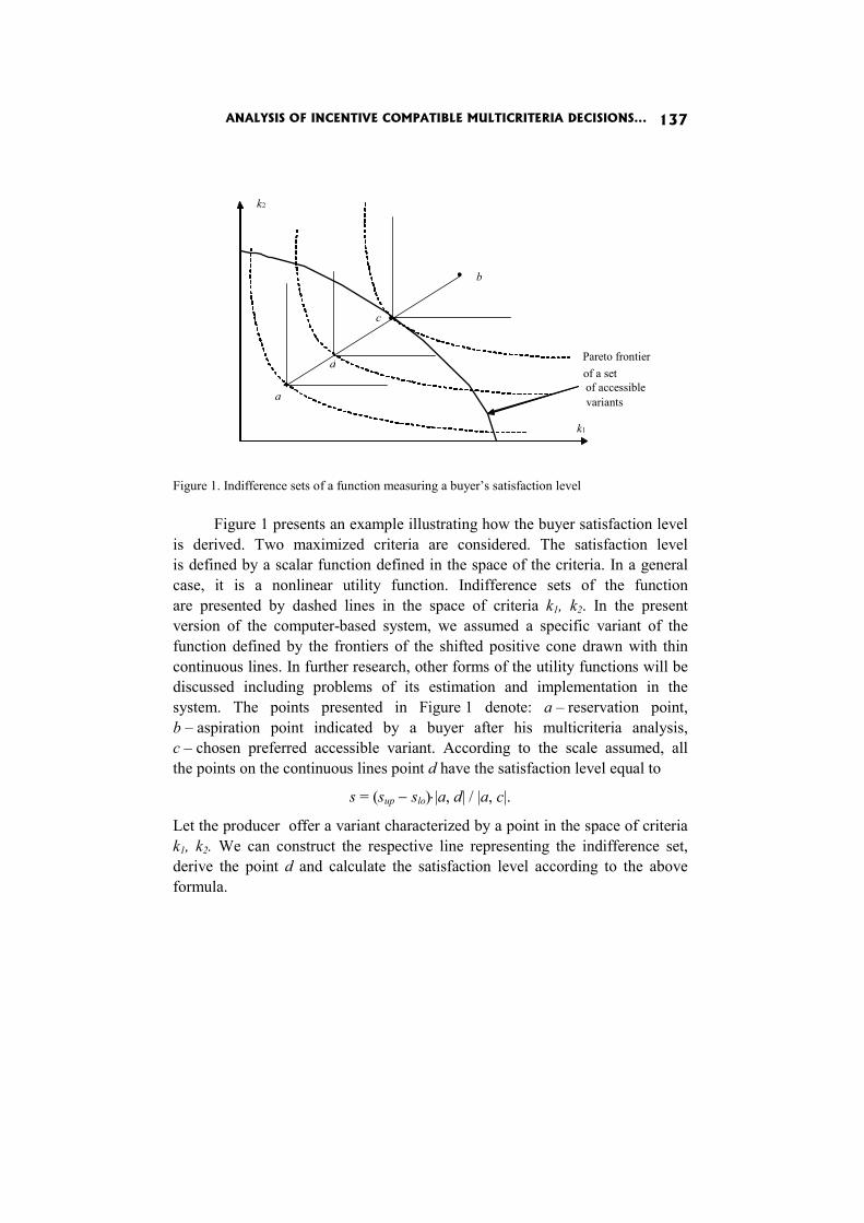
ANALYSIS OF INCENTIVE COMPATIBLE MULTICRITERIA DECISIONS... 137
Figure 1. Indifference sets of a function measuring a buyer’s satisfaction level
Figure 1 presents an example illustrating how the buyer satisfaction level
is derived. Two maximized criteria are considered. The satisfaction level is defined by a scalar function defined in the space of the criteria. In a general case, it is a nonlinear utility function. Indifference sets of the function are presented by dashed lines in the space of criteria k1, k2. In the present version of the computer-based system, we assumed a specific variant of the function defined by the frontiers of the shifted positive cone drawn with thin continuous lines. In further research, other forms of the utility functions will be discussed including problems of its estimation and implementation in the system. The points presented in Figure 1 denote: a – reservation point, b – aspiration point indicated by a buyer after his multicriteria analysis, c – chosen preferred accessible variant. According to the scale assumed, all the points on the continuous lines point d have the satisfaction level equal to
s = (sup − slo)⋅|a, d| / |a, c|.
Let the producer offer a variant characterized by a point in the space of criteria k1, k2. We can construct the respective line representing the indifference set, derive the point d and calculate the satisfaction level according to the above formula.
d
c
k2
k1
•
•
•
a
b
Pareto frontier of a set of accessible variants
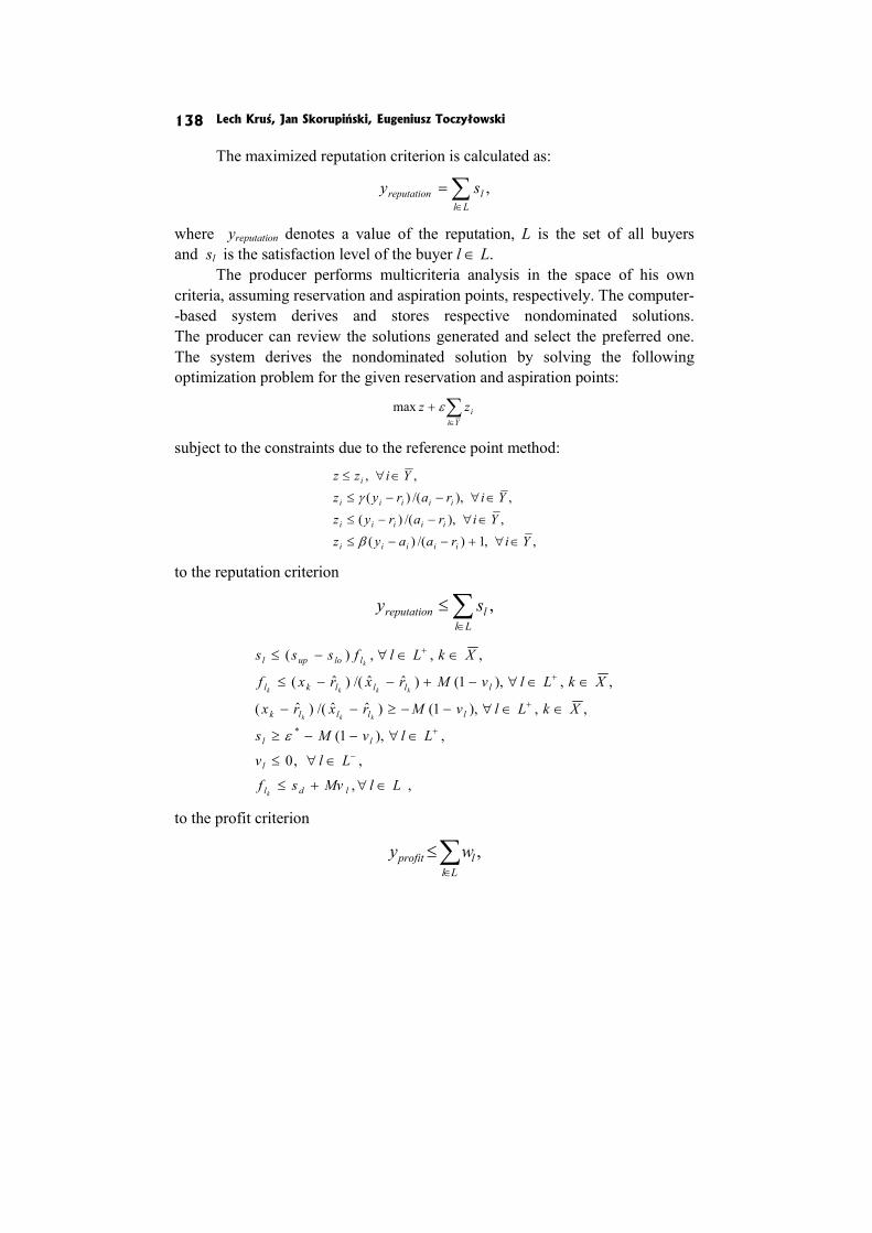
Lech Kruś, Jan Skorupiński, Eugeniusz Toczyłowski 138
The maximized reputation criterion is calculated as:
∑∈
=Ll
lreputation sy ,
where yreputation denotes a value of the reputation, L is the set of all buyers and sl is the satisfaction level of the buyer l ∈ L.
The producer performs multicriteria analysis in the space of his own criteria, assuming reservation and aspiration points, respectively. The computer- -based system derives and stores respective nondominated solutions. The producer can review the solutions generated and select the preferred one. The system derives the nondominated solution by solving the following optimization problem for the given reservation and aspiration points:
∑∈
+Yi
izz εmax
subject to the constraints due to the reference point method:
,,1)/()(,),/()(
,),/()(,,
YiraayzYiraryz
YiraryzYizz
iiiii
iiiii
iiiii
i
∈∀+−−≤
∈∀−−≤
∈∀−−≤
∈∀≤
β
γ
to the reputation criterion
,∑∈
≤Ll
lreputation sy
,,
,,0
,),1(
,,),1()ˆˆ/()ˆ(
,,),1()ˆˆ/()ˆ(
,,,)(
*
LlMvsf
Llv
LlvMs
XkLlvMrxrx
XkLlvMrxrxf
XkLlfsss
ldl
l
ll
llllk
llllkl
lloupl
k
kkk
kkkk
k
∈∀+≤
∈∀≤
∈∀−−≥
∈∈∀−−≥−−
∈∈∀−+−−≤
∈∈∀−≤
−
+
+
+
+
ε
to the profit criterion
,∑∈
≤Ll
lprofit wy
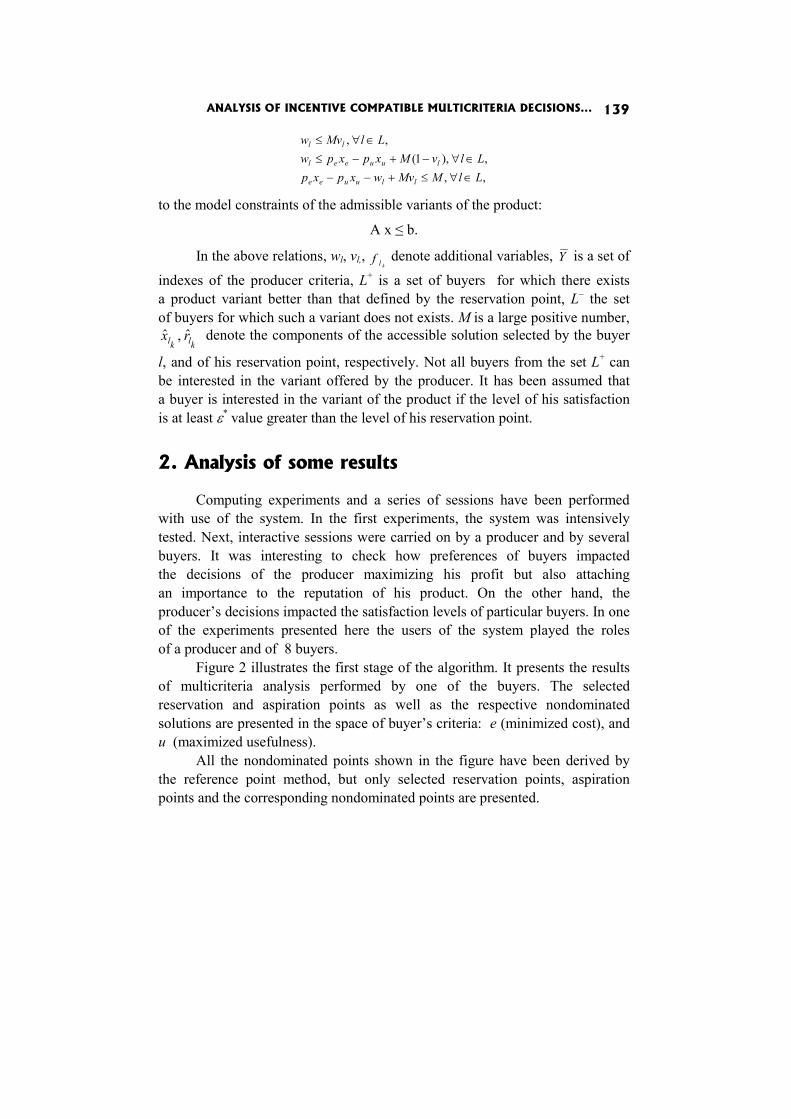
ANALYSIS OF INCENTIVE COMPATIBLE MULTICRITERIA DECISIONS... 139
,,,),1(
,,
LlMMvwxpxpLlvMxpxpw
LlMvw
lluuee
luueel
ll
∈∀≤+−−
∈∀−+−≤∈∀≤
to the model constraints of the admissible variants of the product:
A x ≤ b.
In the above relations, wl, vl,,klf denote additional variables, Y is a set of
indexes of the producer criteria, L+ is a set of buyers for which there exists a product variant better than that defined by the reservation point, L− the set of buyers for which such a variant does not exists. M is a large positive number,
klklrx ˆ,ˆ denote the components of the accessible solution selected by the buyer
l, and of his reservation point, respectively. Not all buyers from the set L+ can be interested in the variant offered by the producer. It has been assumed that a buyer is interested in the variant of the product if the level of his satisfaction is at least ε* value greater than the level of his reservation point.
2. Analysis of some results
Computing experiments and a series of sessions have been performed with use of the system. In the first experiments, the system was intensively tested. Next, interactive sessions were carried on by a producer and by several buyers. It was interesting to check how preferences of buyers impacted the decisions of the producer maximizing his profit but also attaching an importance to the reputation of his product. On the other hand, the producer’s decisions impacted the satisfaction levels of particular buyers. In one of the experiments presented here the users of the system played the roles of a producer and of 8 buyers.
Figure 2 illustrates the first stage of the algorithm. It presents the results of multicriteria analysis performed by one of the buyers. The selected reservation and aspiration points as well as the respective nondominated solutions are presented in the space of buyer’s criteria: e (minimized cost), and u (maximized usefulness).
All the nondominated points shown in the figure have been derived by the reference point method, but only selected reservation points, aspiration points and the corresponding nondominated points are presented.
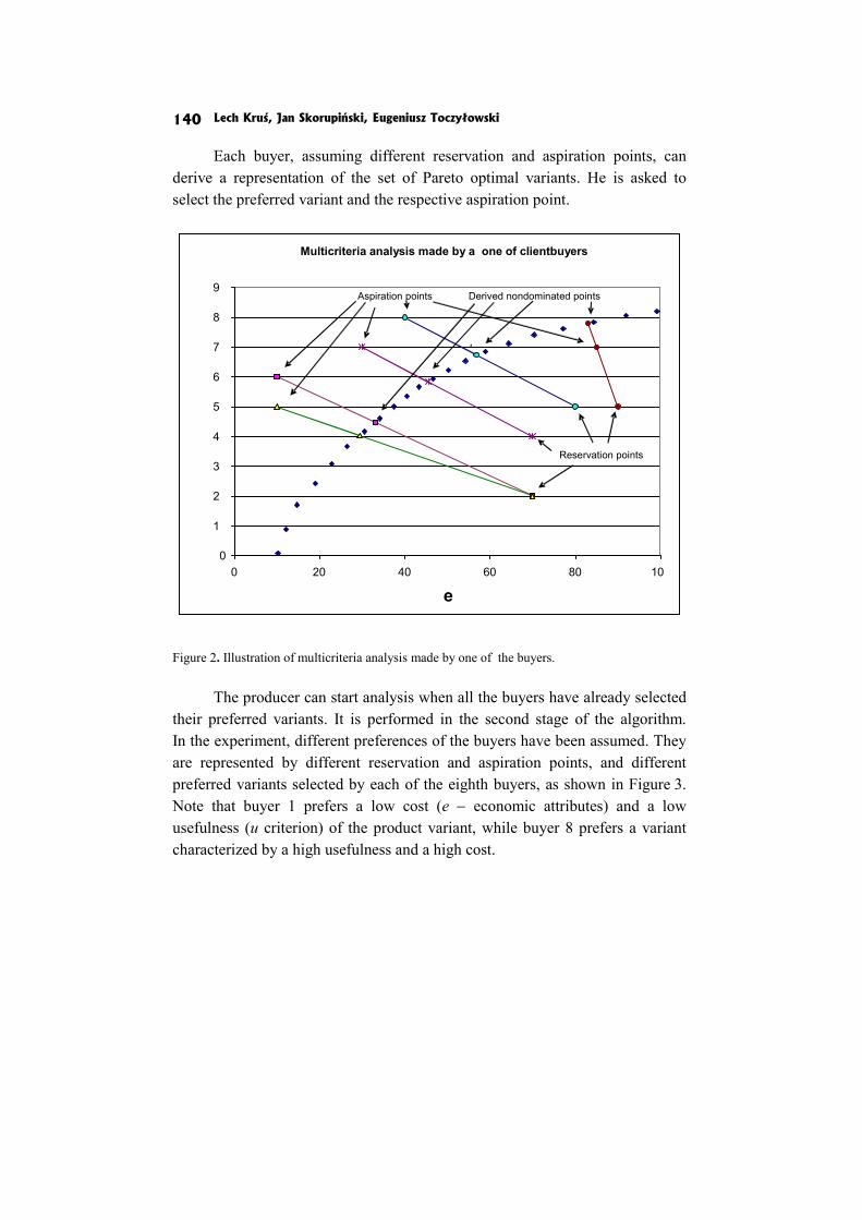
Lech Kruś, Jan Skorupiński, Eugeniusz Toczyłowski 140
Each buyer, assuming different reservation and aspiration points, can derive a representation of the set of Pareto optimal variants. He is asked to select the preferred variant and the respective aspiration point.
Figure 2. Illustration of multicriteria analysis made by one of the buyers. The producer can start analysis when all the buyers have already selected
their preferred variants. It is performed in the second stage of the algorithm. In the experiment, different preferences of the buyers have been assumed. They are represented by different reservation and aspiration points, and different preferred variants selected by each of the eighth buyers, as shown in Figure 3. Note that buyer 1 prefers a low cost (e − economic attributes) and a low usefulness (u criterion) of the product variant, while buyer 8 prefers a variant characterized by a high usefulness and a high cost.
Multicriteria analysis made by a one of clientbuyers
0
1
2
3
4
5
6
7
8
9
0 20 40 60 80 10
e
Aspiration points
Derived nondominated points
k
Reservation points
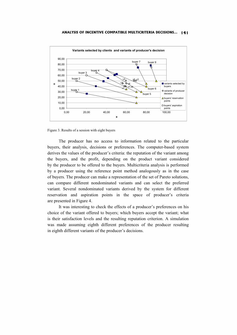
ANALYSIS OF INCENTIVE COMPATIBLE MULTICRITERIA DECISIONS... 141
Figure 3. Results of a session with eight buyers The producer has no access to information related to the particular
buyers, their analysis, decisions or preferences. The computer-based system derives the values of the producer’s criteria: the reputation of the variant among the buyers, and the profit, depending on the product variant considered by the producer to be offered to the buyers. Multicriteria analysis is performed by a producer using the reference point method analogously as in the case of buyers. The producer can make a representation of the set of Pareto solutions, can compare different nondominated variants and can select the preferred variant. Several nondominated variants derived by the system for different reservation and aspiration points in the space of producer’s criteria are presented in Figure 4.
It was interesting to check the effects of a producer’s preferences on his choice of the variant offered to buyers; which buyers accept the variant; what is their satisfaction levels and the resulting reputation criterion. A simulation was made assuming eighth different preferences of the producer resulting in eighth different variants of the producer’s decisions.
Variants selected by clients and variants of producer's decision
0,00
10,00
20,00
30,00
40,00
50,00
60,00
70,00
80,00
90,00
0,00 20,00 40,00 60,00 80,00 100,00
e
u variants selected bybuyers
variants of producerdecision
buyers' reservationpoints
buyers' aspirationpoints
v5 v3 v4v2
buyer 1
buyer 8buyer 7
buyer 6
buyer 5
buyer 4buyer 3
buyer 2
v8v1,v6v7
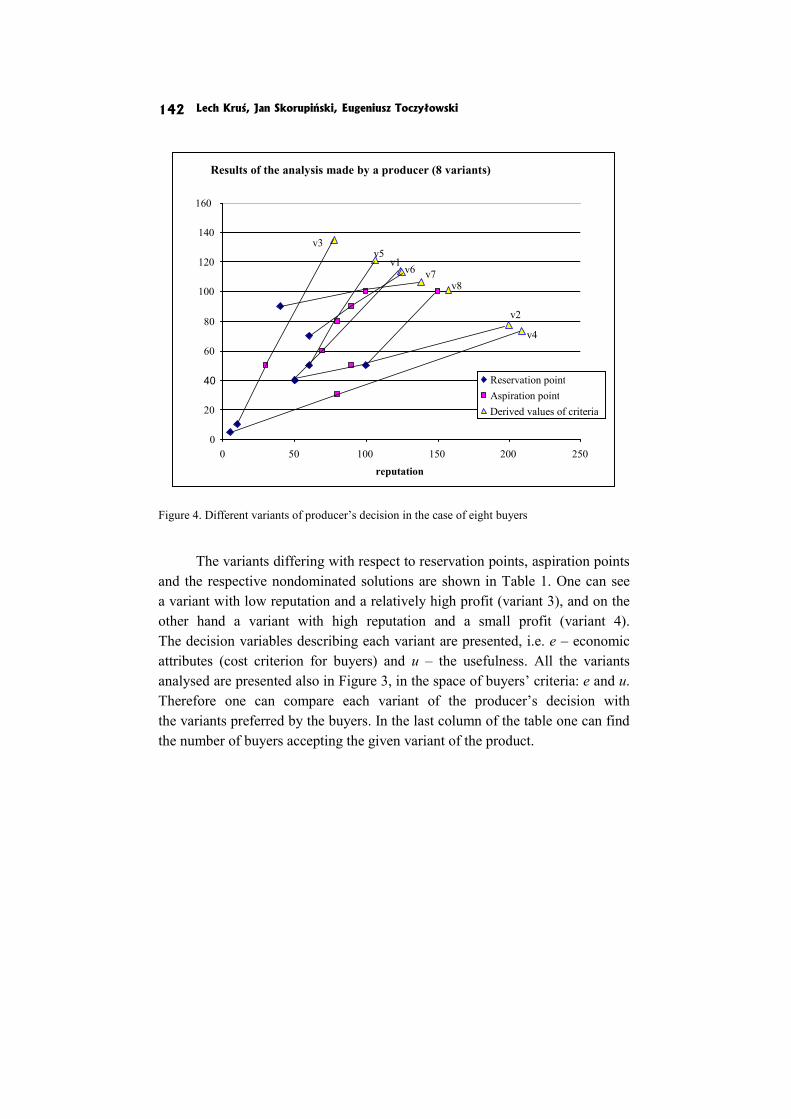
Lech Kruś, Jan Skorupiński, Eugeniusz Toczyłowski 142
Figure 4. Different variants of producer’s decision in the case of eight buyers
The variants differing with respect to reservation points, aspiration points and the respective nondominated solutions are shown in Table 1. One can see a variant with low reputation and a relatively high profit (variant 3), and on the other hand a variant with high reputation and a small profit (variant 4). The decision variables describing each variant are presented, i.e. e – economic attributes (cost criterion for buyers) and u – the usefulness. All the variants analysed are presented also in Figure 3, in the space of buyers’ criteria: e and u. Therefore one can compare each variant of the producer’s decision with the variants preferred by the buyers. In the last column of the table one can find the number of buyers accepting the given variant of the product.
Results of the analysis made by a producer (8 variants)
0
20
40
60
80
100
120
140
160
0 50 100 150 200 250reputation
Reservation pointAspiration pointDerived values of criteria
v4
v3
v2
v5v1
v6v8
v7
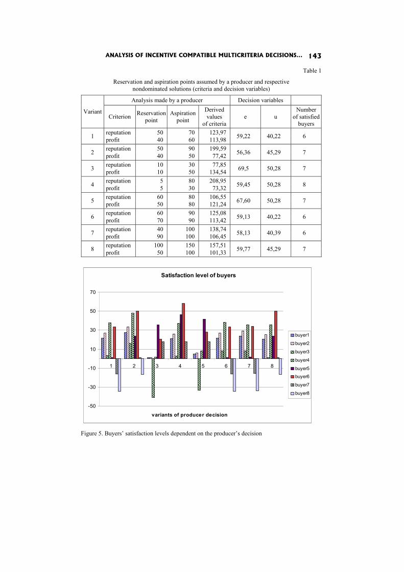
ANALYSIS OF INCENTIVE COMPATIBLE MULTICRITERIA DECISIONS... 143
Table 1
Reservation and aspiration points assumed by a producer and respective nondominated solutions (criteria and decision variables)
Variant
Analysis made by a producer Decision variables
Criterion Reservation point
Aspirationpoint
Derived values
of criteria e u
Number of satisfied
buyers
1 reputation 50 70 123,97 59,22 40,22 6 profit 40 60 113,98
2 reputation 50 90 199,59 56,36 45,29 7 profit 40 50 77,42
3 reputation 10 30 77,85 69,5 50,28 7 profit 10 50 134,54
4 reputation 5 80 208,95 59,45 50,28 8 profit 5 30 73,32
5 reputation 60 80 106,55 67,60 50,28 7 profit 50 80 121,24
6 reputation 60 90 125,08 59,13 40,22 6 profit 70 90 113,42
7 reputation 40 100 138,74 58,13 40,39 6 profit 90 100 106,45
8 reputation 100 150 157,51 59,77 45,29 7 profit 50 100 101,33
Figure 5. Buyers’ satisfaction levels dependent on the producer’s decision
Satisfaction level of buyers
-50
-30
-10
10
30
50
70
1 2 3 4 5 6 7 8
variants of producer decision
buyer1
buyer2
buyer3
buyer4
buyer5
buyer6
buyer7
buyer8
Lech Kruś, Jan Skorupiński, Eugeniusz Toczyłowski 144
Figure 5 shows satisfaction levels of buyers depending on the variants of product offered by the producer. Negative values of the level mean that the respective variant is not accepted by the respective buyers. Variants 1, 6, 7 are not accepted by buyers 7 and 8. Variant 3 and 5 are not accepted by buyer 3. Variant 3 gives the greatest profit to the producer in the set of variants analysed here. The greatest number of buyers is interested in variant 4. This variant has the greatest reputation among buyers but it gives the lowest profit to the producer.
Conclusions
A mathematical model describing the producer and buyers problem has been proposed. It includes formulations of optimization tasks solved during the multicriteria analysis conducted by the buyers and by the producer. The optimization tasks have been implemented in a specially designed multiagent computer-based system.
An original proposal for the derivation of satisfaction levels of individual buyers is presented. On this basis, the reputation can be calculated. It is one of the producer’s criteria. It reconciles the producer’s and buyers’ interests. The buyer’s satisfaction level is derived with use of the BATNA concept and with use of an assumed form of the buyer’s utility function. In further research, different ways of the derivation will be analyzed. In particular, different forms of the utility function and interactive procedures for scaling the function with use of information obtained from buyers will be discussed.
The multiagent computer-based system enables buyers and producers to perform multicriteria analysis in two stages. An experiment with human users of the system, playing the roles of a producer and 8 buyers, illustrates the method. It is shown how the variant proposed to the buyers depends on the producer’s preferences and how it is seen by the buyers.
Acknowledgement
The research is partially supported by the Ministry of Science and Higher Education in Poland, Grant No. N N514 044438.
ANALYSIS OF INCENTIVE COMPATIBLE MULTICRITERIA DECISIONS... 145
References
AIMMS − Optimization Software for Operations Research Applications, www. aimms.com.
Bisschop J., Roelofs M. (2009), The AIMMS Language Reference, Paragon Decision Technology.
Coombs C.H; Dawes R.M, Tversky A. (1970), Mathematical Psychology: An Elemen-tary Introduction, Prentice-Hall, Oxford.
Fisher R., Ury W. (1981), Getting to Yes, Hougton Mifflin, Boston. Kruś L. (2002), Multicriteria Decision Support in Bargaining, a Problem of Players
Manipulations, [in:] Multiple Objective and Goal Programming, eds T. Trzas-kalik, J. Michnik, Physica Verlag, Springer, Berlin.
Kruś L. (2004), A Multicriteria Approach to Cooperation in the Case of Innovative Activity, “Control and Cybernetics”, Vol. 33, No. 3.
Kruś L. (2008), On Some Procedures Supporting Multicriteria Cooperative Decisions, “Foundations of Computing and Decision Science”, Vol. 33 (3).
Raiffa H. (1982), The Art and Science of Negotiations, Harvard University Press, Cam-bridge.
Skorupiński J. (2010), Wieloagentowy system komputerowy wspomagający wielo-kryterialną analizę w problemie producenta i klientów (Multi Agent Computer- -based System Supporting Multicriteria Analysis in a Producer and Buyers Problem), Eng. Diploma Thesis, IAiIS Warsaw University of Techn., Warszawa.
Toczyłowski E. (2003), Optymalizacja procesów rynkowych przy ograniczeniach (Optimization of Market Processes Subject to Constraints), AOW EXIT, War-szawa.
Toczyłowski E. (2009), Zgodność motywacji w mechanizmach rynku energii (Incentive Compatibility in Mechanism of Energy Market), “Rynek Energii”, nr II(IV).
Torgerson W.S. (1958), Theory and Methods of Scaling, Wiley, New York. Wierzbicki A.P. (1986), On the Completeness and Constructiveness of Parametric
Characterizations to Vector Optimization Problems, OR Spectrum, Vol. 8, 73- -87, Springer Verlag.
Wierzbicki A.P., Krus L., Makowski M. (1993), The Role of Multi-Objective Optimi-zation in Negotiation and Mediation Support. Theory and Decision, special issue on “International Negotiation Support Systems: Theory, Methods, and Practice”, Vol. 34, (2).
Wierzbicki A.P., Makowski M., Wessels J. (2000), Model-based Decision Support Methodology with Environmental Applications, Kluwer Academic Press, Dordrecht, Boston.
Bogumiła Krzeszowska
MULTIPLE CRITERIA PROJECT SCHEDULING WITH PROJECT DELAY, RESOURCE LEVEL AND NPV OPTIMIZATION
Abstract
One of the most important phases in project management is planning. During this phase tasks are identified and scheduled. A schedule brings information on how tasks should be planned over time during the realization phase of the project. That is why scheduling is a critical issue in project management. The main project scheduling techniques are CPM and PERT. They deliver the schedule with the optimal project finish time and ensure the control of resource usage. In real-life applications the schedule should optimize not only the project finish time but also resource usage and cash flows. In research on the project scheduling problem the mathematical models are used to build an optimal project schedule. Frequently used are one-objective mathematical models for project scheduling. Few papers deal with the multiple objective project scheduling problem. Constraints and objectives in project scheduling are determined by three main issues: time, resource and costs, but only few papers consider all of them.
A zero-one programming formulation has been applied to solve a multiple criteria project scheduling problem in this paper. The purpose of this paper is to present the multiple criteria project scheduling problem with three objectives: project delay minimization, resource usage in each period of time minimization and NPV maximization.
Keywords
Project scheduling, multiple criteria optimization, zero-one programming.
Introduction
In recent years the project management problem became very popular because of its broad real-life applications. One of project definitions states that a project is a set of co-ordinated activities undertaken to meet specific objectives [Brandenburg 2002]. Each project has three main components: activities (tasks to do), resources required to carry out the project tasks,
MULTIPLE CRITERIA PROJECT SCHEDULING WITH PROJECT DELAY... 147
and precedence relationships, which define the order in which activities should be performed [Kostrubiec 2003]. In summary: a project contains activities, which have an expected duration and resource requirements. They generate costs and cash flows and are constrained by resource limits and precedence relationships. In real-life applications a schedule should hold all those restrictions. That is why scheduling is a critical task in project management.
In project management, a schedule consists of a list of a project's terminal elements with intended start and finish dates. We can say that: “(…) scheduling is to forecast the processing of work by assigning resources to tasks and fixing their start times. (…) The different components of a scheduling problem are tasks, the potential constraints, the resources and the objective…” [Carlier and Chretienne 1988]. “Scheduling concerns the allocation of limited resources to tasks over time. It is a decision-making process that has a goal − the optimi-zation of one or more objectives” [Pinedo 1995]. The main project scheduling techniques are CPM and PERT. CPM calculates the longest path of planned activities to the end of the project and also gives the shortest time of project realization. The Program Evaluation and Review Techniques (PERT) is a method to analyze the tasks involved in completing a given project, especially the time needed to complete each task. Those methods deliver schedules with the optimal project finish time and ensure the control of resource usage. In real-life applications the schedule should optimize not only the project finish time but also resource usage and cash flows.
The purpose of this paper is to analyze the problem of multiple criteria project scheduling problem and to discuss the multiple criteria project scheduling problem with three objectives: project delay minimization, minimi-zation of resource usage in each period of time and NPV maximization. A zero- -one programming approach has been applied to model such a problem.
The paper begins with an overview of literature and problem statement. Then, the mathematical model is described and a computational example is presented. The paper finishes with conclusions and ideas for future research.
1. Optimization in project scheduling problem – a literature overview
Constraints in project scheduling problem are determined by two main components: time and resources. We can discuss two types of resources: financial and non-financial (human resources and materials). The optimization criteria are determined by three main components: time, resources and eco-nomic indicators such as cost or NPV. When we take them into consideration
Bogumiła Krzeszowska 148
we can build various optimization models for the project scheduling problem. We can also present various projects depending on the number of objectives, thus we can have a one-objective project scheduling problem and a multiple-criteria project scheduling problem.
Each mathematical model for project scheduling problem needs to include basic constraints: precedence relationship constraints and information about the extent of variables.
In research on project scheduling problems, optimization models with one objective are the most popular. In this case we can build a model containing only basic constraints, in which the project completion time or NPV is optimized, or a model with one constraint in which time, capital or resources are constrained while the project completion time, NPV, cost or resource usage are optimized, or a model with few constraints. A resource constraint is not frequently used in models with resource usage optimization. A multiple objective mathematical model for the project scheduling problem is a combi-nation of mathematical models mentioned above.
A problem with only basic constraints in which NPV is maximized has been solved by Russell [Russell 1970]. In this paper the author assumed that the cost is generated at the moment when the project starts and income is generated when some groups of activities are finished.
There are two types of mathematical models for the project scheduling problem with one constraint: the time constrained project scheduling problem and the resource constrained project scheduling problem. In the case of the resource constrained project scheduling problem we can differentiate between problems with non-financial resources and those with capital constraints.
The project scheduling problem with time constraints where NPV is maximized has been presented in the paper by Vanhoucke, Demeulemeester and Herrorlen [Vanhoucke et al. 2002]. In the problem described in the paper cash flows were generated at the time when each activity was finished.
There are two types of the resource constrained project scheduling problems: resource constrained project scheduling problem with time optimi-zation and resource constrained project scheduling problem with NPV optimization.
The resource constrained project scheduling problem with time optimi-zation was discussed by Shouman, Ibrahim, Khater and Forgani [Shouman et al. 2006] and the problem with NPV optimization was presented by Icmeli and Erenguc [Icmeli and Erenguc 1996]. The resource constrained project scheduling problem was also described in Talbot’s paper [Talbot 1982]. The author presented this problem with time-resource tradeoffs.
MULTIPLE CRITERIA PROJECT SCHEDULING WITH PROJECT DELAY... 149
Doersch and Patterson [Doersch and Patterson 1977] proposed a financial resources (capital) constrained project scheduling problem in their paper. They assumed that the capital is limited at the project start time. The capital availability changes throughout the project duration. Activities generate cash flows (outflows and inflows), which have influence on capital availability.
Vanhoucke, Demeulemeester and Herroelen [Vanhoucke et al. 2001] described a time- and resource-constrained project scheduling problem with NPV maximization.
A resource- and time-constrained project scheduling problem was also presented by Bartusch, Mohring and Readermacher [Bartusch et al. 1988]. A vector containing the finish time of each activity is minimized. The authors assumed that an activity should start in the “time window”, which is the time between the earliest and the latest start times.
Bianco, Dell`Olmo and Speranza [Bianco et al. 1998] described resource- -constrained project scheduling problems with financial and non-financial resources. Each activity can be executed in several ways. Additionally, each activity generates a given cost. The project budget is limited. Additionally, activities using the same resource cannot be scheduled at the same time. The project completion time is optimized in this problem.
Gaspars-Wieloch [Gaspars-Wieloch 2008] presented a paper on time and cost analysis for the project scheduling problem. The author considered a few mathematical models from the literature on this problem. In the models considered both time and cost can be a constraint and an objective function.
A multiple criteria project scheduling problem was described by Viana and de Sousa [Viana and Sousa 2000]. The authors proposed a mathematical model in which: project completion times are minimized, project delay is minimized and disruptions in resource usage are minimized. Renewable and nonrenewable resources are constrained in the problem. A binary variable is used in the model. We define xijt = 1 when the operation j of the activity i is finished in time t. Otherwise, xijt = 0.
Leu and Yang [Leu and Yang 1999] considered a multiple-criteria resource-constrained project scheduling problem with time optimization, cost optimization and resource usage optimization. Also Hapke, Jaszkiewicz and Słowiński [Hapke et al. 1998] described that problem in their paper.

Bogumiła Krzeszowska 150
2. Project scheduling problem – basic elements
of the model
The problem presented in this paper can be formulated as follows: there is a project to be scheduled. By ‘scheduling’ we understand setting the start and finish times of each activity. For each activity, resource requirements and budget are specified. Resource availability and precedence relationships are constrained.
The following example (Figure 1) describes the problem presented in this paper. We have a project containing 9 activities. The project is presented by an AOA (Activity On Arc) network. For each activity, its duration, required resources and net cash flows generated are shown in Table 1.
Figure 1. Activity network for example 1 For given durations and precedence relationships, the earliest start and
finish times and the latest start and finish times were computed using the critical path method. Those times will be compared with the results obtained by using the mathematical model proposed in this paper.
Table 1
Example 1. Data
Activity Duration ES EF LS LF Slack Critical tasks?
Renewable resources Net cash flow
1 2 3 4 5 6 7 8 9 10 1-2 2 0 2 0 2 0 YES 2 −4 1-3 4 0 4 1 5 1 NO 1 −3
1
2
3
4
5
7
8
6
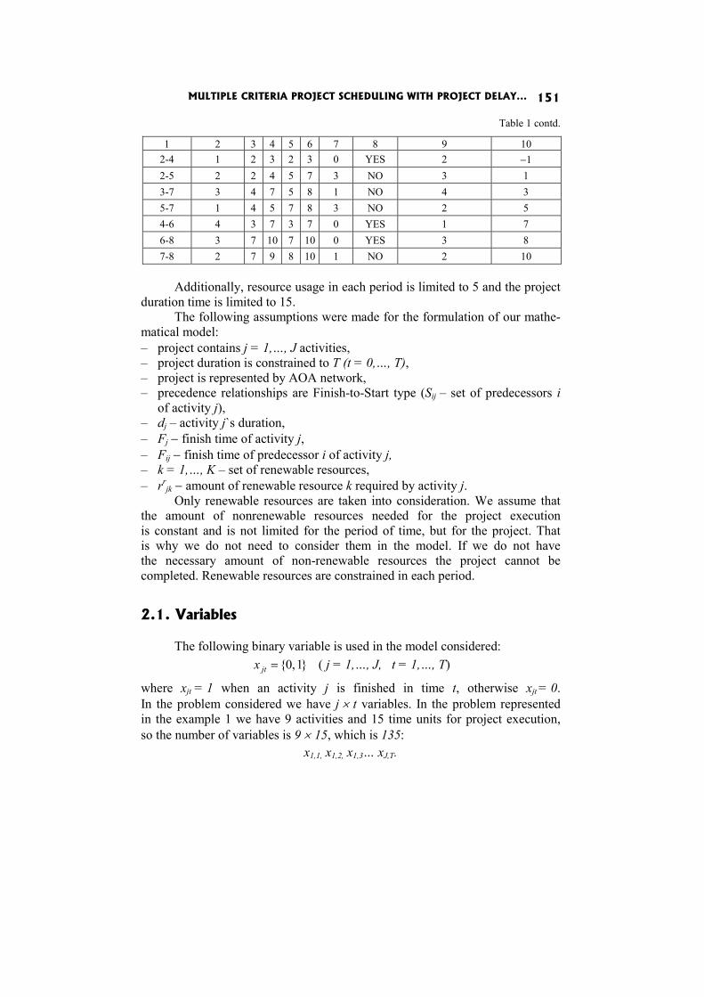
MULTIPLE CRITERIA PROJECT SCHEDULING WITH PROJECT DELAY... 151
Table 1 contd.
1 2 3 4 5 6 7 8 9 10 2-4 1 2 3 2 3 0 YES 2 −1 2-5 2 2 4 5 7 3 NO 3 1 3-7 3 4 7 5 8 1 NO 4 3 5-7 1 4 5 7 8 3 NO 2 5 4-6 4 3 7 3 7 0 YES 1 7 6-8 3 7 10 7 10 0 YES 3 8 7-8 2 7 9 8 10 1 NO 2 10
Additionally, resource usage in each period is limited to 5 and the project
duration time is limited to 15. The following assumptions were made for the formulation of our mathe-
matical model: – project contains j = 1,…, J activities, – project duration is constrained to T (t = 0,…, T), – project is represented by AOA network, – precedence relationships are Finish-to-Start type (Sij – set of predecessors i
of activity j), – dj – activity j`s duration, – Fj − finish time of activity j, – Fij − finish time of predecessor i of activity j, – k = 1,…, K – set of renewable resources, – rr
jk − amount of renewable resource k required by activity j. Only renewable resources are taken into consideration. We assume that
the amount of nonrenewable resources needed for the project execution is constant and is not limited for the period of time, but for the project. That is why we do not need to consider them in the model. If we do not have the necessary amount of non-renewable resources the project cannot be completed. Renewable resources are constrained in each period.
2.1. Variables
The following binary variable is used in the model considered: }1,0{=jtx ( j = 1,…, J, t = 1,…, T)
where xjt = 1 when an activity j is finished in time t, otherwise xjt = 0. In the problem considered we have j × t variables. In the problem represented in the example 1 we have 9 activities and 15 time units for project execution, so the number of variables is 9 × 15, which is 135:
x1,1, x1,2, x1,3… xJ,T.

Bogumiła Krzeszowska 152
2.2. An activity execution constraint
Because a binary variable is used in the model formulated, we have to ensure that each activity will be executed only once. We will write this constraint as the following equation:
11
=∑=
T
tjtx ( j = 1,…, J, t = 1,…, T)
In the equation above we add the variables in each time unit for each activity. If the sum is equal 1 we are sure, that an activity j is finished only once.
In example 1 this constraint is formulated as follows (for the activity 1-2):
x1,1+ x1,2+ x1,3+ x1,4+ x1,5+ x1,6+ x1,7+ x1,8+ x1,9+ x1,10+ x1,11+ x1,12+ x1,13+ x1,14+ x1,15 = 1.
2.3. Precedence relationships
The project scheduling problem considered in this paper has been pre-sented by an AOA network. This network allows to consider only finish-to-start precedence relationships between activities. This type of precedence relation-ships can be formulated as follows:
ijjj FdF ≥− ( j = 1,…, J, t = 1,…T, I ∈ Sij)
In this case a successor can start only when its predecessor is finished. In example 1 activity 2-4 can start when activity 1-2 is finished, so the set
Sij of predecessors i of activity j has only one element. The precedence relationship for this case can be formulated as follows:
122 FdF ≥− .
In the case of precedence relationships we use activity finish time. We can calculate activity finish times by using the formula:
)}(max{,..,1 jtTtj xtF ×∀=
=. So, the finish time for the activity 1-2 is:
F1 = max{1× x1,1, 2× x1,2, 3× x1,3, 4× x1,4, 5× x1,5, 6× x1,6, 7× x1,7, 8× x1,8, 9× x1,9, 10× x1,10, 11× x1,11, 12×x1,12, 13× x1,13, 14× x1,14, 15× x1,15}.
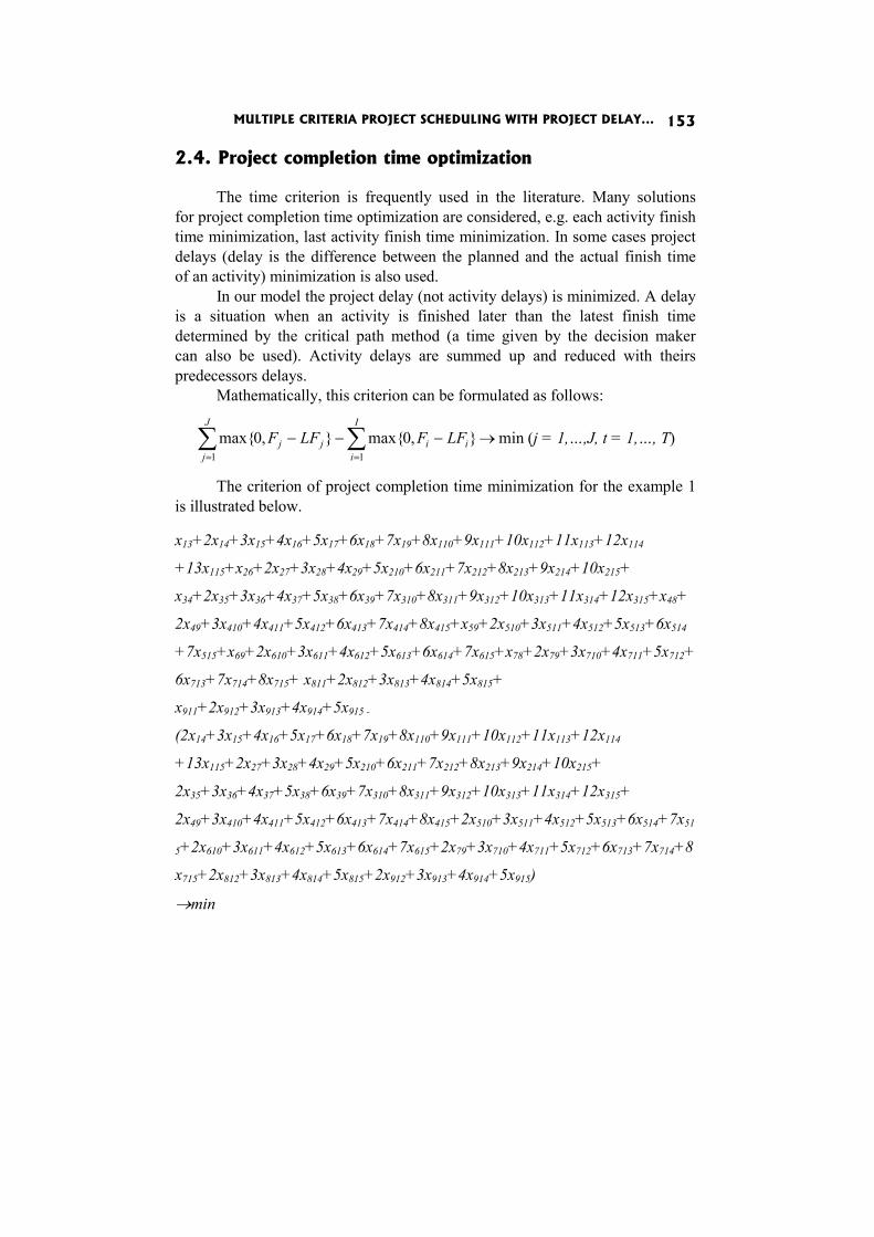
MULTIPLE CRITERIA PROJECT SCHEDULING WITH PROJECT DELAY... 153
2.4. Project completion time optimization
The time criterion is frequently used in the literature. Many solutions for project completion time optimization are considered, e.g. each activity finish time minimization, last activity finish time minimization. In some cases project delays (delay is the difference between the planned and the actual finish time of an activity) minimization is also used.
In our model the project delay (not activity delays) is minimized. A delay is a situation when an activity is finished later than the latest finish time determined by the critical path method (a time given by the decision maker can also be used). Activity delays are summed up and reduced with theirs predecessors delays.
Mathematically, this criterion can be formulated as follows:
min},0max{},0max{11
→−−− ∑∑==
i
I
iij
J
jj LFFLFF (j = 1,…,J, t = 1,…, T)
The criterion of project completion time minimization for the example 1 is illustrated below.
x13+2x14+3x15+4x16+5x17+6x18+7x19+8x110+9x111+10x112+11x113+12x114
+13x115+x26+2x27+3x28+4x29+5x210+6x211+7x212+8x213+9x214+10x215+
x34+2x35+3x36+4x37+5x38+6x39+7x310+8x311+9x312+10x313+11x314+12x315+x48+
2x49+3x410+4x411+5x412+6x413+7x414+8x415+x59+2x510+3x511+4x512+5x513+6x514
+7x515+x69+2x610+3x611+4x612+5x613+6x614+7x615+x78+2x79+3x710+4x711+5x712+
6x713+7x714+8x715+ x811+2x812+3x813+4x814+5x815+
x911+2x912+3x913+4x914+5x915 -
(2x14+3x15+4x16+5x17+6x18+7x19+8x110+9x111+10x112+11x113+12x114
+13x115+2x27+3x28+4x29+5x210+6x211+7x212+8x213+9x214+10x215+
2x35+3x36+4x37+5x38+6x39+7x310+8x311+9x312+10x313+11x314+12x315+
2x49+3x410+4x411+5x412+6x413+7x414+8x415+2x510+3x511+4x512+5x513+6x514+7x51
5+2x610+3x611+4x612+5x613+6x614+7x615+2x79+3x710+4x711+5x712+6x713+7x714+8
x715+2x812+3x813+4x814+5x815+2x912+3x913+4x914+5x915)
→min
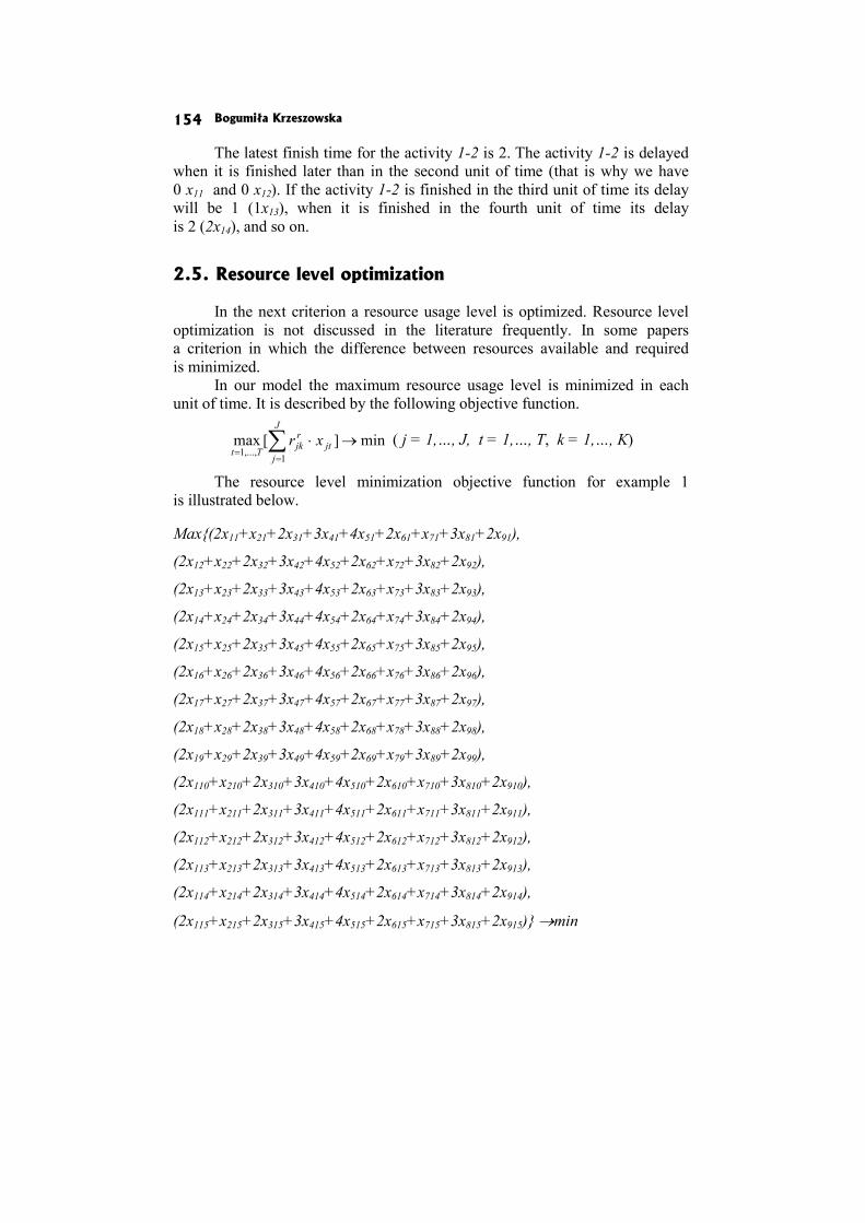
Bogumiła Krzeszowska 154
The latest finish time for the activity 1-2 is 2. The activity 1-2 is delayed when it is finished later than in the second unit of time (that is why we have 0 x11 and 0 x12). If the activity 1-2 is finished in the third unit of time its delay will be 1 (1x13), when it is finished in the fourth unit of time its delay is 2 (2x14), and so on.
2.5. Resource level optimization
In the next criterion a resource usage level is optimized. Resource level optimization is not discussed in the literature frequently. In some papers a criterion in which the difference between resources available and required is minimized.
In our model the maximum resource usage level is minimized in each unit of time. It is described by the following objective function.
min][max1,...,1
→⋅∑=
=jt
J
j
rjkTt
xr ( j = 1,…, J, t = 1,…, T, k = 1,…, K)
The resource level minimization objective function for example 1
is illustrated below.
Max{(2x11+x21+2x31+3x41+4x51+2x61+x71+3x81+2x91),
(2x12+x22+2x32+3x42+4x52+2x62+x72+3x82+2x92),
(2x13+x23+2x33+3x43+4x53+2x63+x73+3x83+2x93),
(2x14+x24+2x34+3x44+4x54+2x64+x74+3x84+2x94),
(2x15+x25+2x35+3x45+4x55+2x65+x75+3x85+2x95),
(2x16+x26+2x36+3x46+4x56+2x66+x76+3x86+2x96),
(2x17+x27+2x37+3x47+4x57+2x67+x77+3x87+2x97),
(2x18+x28+2x38+3x48+4x58+2x68+x78+3x88+2x98),
(2x19+x29+2x39+3x49+4x59+2x69+x79+3x89+2x99),
(2x110+x210+2x310+3x410+4x510+2x610+x710+3x810+2x910),
(2x111+x211+2x311+3x411+4x511+2x611+x711+3x811+2x911),
(2x112+x212+2x312+3x412+4x512+2x612+x712+3x812+2x912),
(2x113+x213+2x313+3x413+4x513+2x613+x713+3x813+2x913),
(2x114+x214+2x314+3x414+4x514+2x614+x714+3x814+2x914),
(2x115+x215+2x315+3x415+4x515+2x615+x715+3x815+2x915)} →min

MULTIPLE CRITERIA PROJECT SCHEDULING WITH PROJECT DELAY... 155
The resources required are multiplied by the binary variable and summed up in each time unit. Then the maximum value is chosen. Resources are used only when the variable is 1.
2.6. NPV optimization
The next criterion presented in this paper is the NPV maximization. Cash flow depends on activity duration and finish time.
This problem is frequently discussed in the literature. An example is considered in Icmeli and Erenguc’s paper [Icmeli and Erenguc 1996]. There, cash flows are generated in each unit of time of activity duration. This problem can be formulated as follows:
.max]][[ )(
11
→⋅⋅ −−
==∑∑ jj
jFtd
d
tjt
J
i
eecf αα
In our paper we assume that cash flows are generated by activities at the end of their durations, so the criterion can be formulated as follows:
max1
→⋅∑=
−J
j
Fj
jecf α ( j = 1,…,J, t = 1,…, T)
In example 1 this criterion has the following form:
.max987
6514321
987
654321
→⋅+⋅+⋅+
⋅+⋅+⋅+⋅+⋅+⋅−−−
−−−−−−
FFF
FFFFFF
ecfecfecf
ecfecfecfecfecfecfααα
αααααα
3. Multiple objective project scheduling problem
We can build various one-objective optimization models for the project scheduling problem using the criterion and constraints considered above. In some cases the objective function can be presented as a constraint, e.g. a resource constraint can be formulated as follows:
ktjt
J
j
rjkTt
Rxr ≤⋅∑=
=][max
1,...,1
.
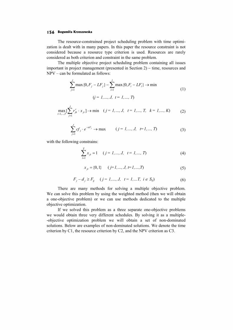
Bogumiła Krzeszowska 156
The resource-constrained project scheduling problem with time optimi-zation is dealt with in many papers. In this paper the resource constraint is not considered because a resource type criterion is used. Resources are rarely considered as both criterion and constraint in the same problem.
The multiple objective project scheduling problem containing all issues important in project management (presented in Section 2) − time, resources and NPV – can be formulated as follows:
min},0max{},0max{11
→−−− ∑∑==
i
I
iij
J
jj LFFLFF
(j = 1,…, J, t = 1,…, T)
(1)
min][max1
,...,1→⋅∑
==
jt
J
j
rjkTt
xr ( j = 1,…, J, t = 1,…, T, k = 1,…, K)
(2)
max1
→⋅∑=
−J
j
Fj
jecf α ( j = 1,…, J, t=1,…, T)
(3)
with the following constrains:
11
=∑=
T
tjtx
( j = 1,…, J, t = 1,…, T) (4)
}1,0{=jtx ( j=1,…, J, t=1,…,T) (5)
ijjj FdF ≥− ( j = 1,…, J, t = 1,…T, i ∈ Sij) (6)
There are many methods for solving a multiple objective problem. We can solve this problem by using the weighted method (then we will obtain a one-objective problem) or we can use methods dedicated to the multiple objective optimization.
If we solved this problem as a three separate one-objective problems we would obtain three very different schedules. By solving it as a multiple- -objective optimization problem we will obtain a set of non-dominated solutions. Below are examples of non-dominated solutions. We denote the time criterion by C1, the resource criterion by C2, and the NPV criterion as C3.
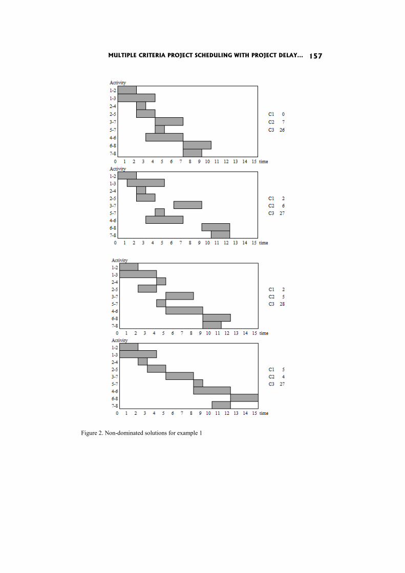
MULTIPLE CRITERIA PROJECT SCHEDULING WITH PROJECT DELAY... 157
Figure 2. Non-dominated solutions for example 1
Bogumiła Krzeszowska 158
Four non-dominated solutions are presented above (Figure 2). We can see that the value of time criterion is between 0 (project finished on time) and 5 (project 5 time units delayed), of resource criterion is between 4 and 7 (the maximum level of resource usage) and of NPV is between 26 and 27 (Table 2).
Table 2
Example 1. Non-dominated solutions − criteria values
S1 S2 S3 S4 C1 0 2 2 5 C2 7 6 5 4 C3 26 27 28 27 Project delay and resource usage are strongly connected with each other.
When resource usage level is decreasing then project delay is increasing. The result of multiple objective problem is a set of non-dominated
solutions. In this case four of them were identified. But in the cases of larger projects the number of non-dominated solutions can be much larger. Then the preferential information of the decision maker about the schedules should be considered and one schedule should be chosen.
Conclusions
The type of constrains and optimization criteria in the project scheduling problem are determined by three main components: time, resource and capital.
By using multiple criteria optimization models in the project scheduling problem we can create an optimal project schedule because it is expressed not only in terms of time, but also in terms of resource usage or project’s NPV.
A zero-one programming approach for project scheduling problem has been presented in this paper.
An advantage of this approach is its form. A binary variable is easy to use and adapt to include new objectives related to the needs. The indicators of project schedule obtained from objective functions deliver clear information about project realization, e.g. an objective function in time optimization gives a concrete number, which is the project delay.
A disadvantage of model proposed is its large number of variables, namely j × t. In the case of larger projects or larger planning horizon the number of variables will be huge.
MULTIPLE CRITERIA PROJECT SCHEDULING WITH PROJECT DELAY... 159
In future research other mathematical models for project scheduling problem should be considered, e.g. mathematical model in which, variables present finish times of activities or mathematical model with binary variables in which xjt = 1 when an activity j last in period t.
Algorithms for solving this problem should be considered. The objective functions are nonlinear, so heuristic methods should be considered as a method of solution. Binary variables enable to use genetic algorithms.
In future research Activity-On-Node network should be considered. When representing the project scheduling problem by an AON network we can use not only finish-to-start precedence relationship but also other types of precedence relationships, such as: start-to-finish, start-to-start or finish-to- -finish.
References
Bartusch M., Mohring R., Radermacher F. (1988), Scheduling Project Networks with Resource Constraints and Time Windows, “Annals of Operations Research”, No. 16(1-4).
Bianco L., Dell`Olmo P., Speranza M. (1998), Heuristics for Multimode Scheduling Problem with Dedicated Resources, “European Journal of Operational Re-search”, No. 107.
Brandenburg H. (2002), Project Management, University of Economics in Katowice Publisher, Katowice.
Carlier J., Chrétienne P. (1988), Problèmes d’ordonnancement: modélisation /complexité/algorithmes, Masson, Paris.
Doersch R.H., Patterson J.H. (1977), Scheduling a Project to Maximize its Present Value: a Zero-one Programming Approach, “Management Science”, No. 23(8).
Gaspars-Wieloch H. (2008), Optimization Models for Time and Cost Analysis Review, [in:] An Operational Research Department Works, ed. W. Sikora, University of Economics, Poznań.
Hapke M., Jaszkiewiecz A., Słowiński R. (1998), Interactive Analysis of Multiple- -criteria Project Scheduling Problems, “European Journal of Operational Research, No. 107.
Icmeli O., Erenguc S.S. (1996), A Branch and Bound Procedure for the Resource Constrained Project Scheduling Problem with Discounted Cash Flows, “Management Science”, No. 42(10).
Kostrubiec A. (2003), Project Scheduling − Models Review, [in:] Project Management Engineering, ed. L. Zawadzka, Gdańsk.
Bogumiła Krzeszowska 160
Leu S.S,., Yang C.H. (1999), Ga-based Multicriteria Optimal Model for Construction Scheduling, “Journal of Construction Engineering and Management”, No. 125(6).
Pinedo M. (1995), Scheduling – Theory, Algorithms and Systems, Prentice Hall Engle-wood Cliffs.
Russell R.A. (1970), Cash Flows in Networks, “Management Science”, No. 16(5). Shouman M.A., Ibrahim M.S., Khater M., Forgani A.A. (2006), Genetic Algorithm
Constraint Project Scheduling, “Alexandria Engineering Journal”, Vol. 45, No. 3.
Talbot T. (1982), Resource-constrained Project Scheduling with Time-resource Trade-offs: The Non-preemptive, “Management Science”, Vol. 28, Iss. 10.
Vanhoucke M., Demeulemeester E., Herroelen W. (2001), On Maximizing the Net Present Value of a Project Under Renewable Resource Constraints, “Mana-gement Science”, No. 47(8).
Vanhoucke M., Demeulemeester E., Herroelen W. (2002), Progress Payments in Pro-ject Scheduling Problems, “European Journal of Operational Research”, No. 148.
Viana A., de Sousa J.P. (2000), Using Metaheuristic in Multiobjective Resource Constrained Project Scheduling, “European Journal of Operational Research”, No. 120.

Jerzy Michnik
WHAT KINDS OF HYBRID MODELS ARE USED IN MULTIPLE CRITERIA DECISION ANALYSIS AND WHY?*
Abstract
Currently, a growing number of papers presenting the hybrid models in the field of MCDA is observed. In this paper we try to explain the reasons for the growing popularity of hybrid models. The most important question considers the reasons for the use of these, rather complicated, structures. We also try to find out the differences between various models which are called hybrid.
Keywords
Discrete models, hybrid models, hybrid solvers, integrated models, multiple criteria decision analysis (MCDA), mixed models.
Introduction
If one reviews MCDA literature, it seems that the term “hybrid” became popular in the beginning of the 21st century. However, it is clear that mixed methods had been used earlier for many years without being named as such. The authors used other terms such as integrated or mixed models. In many cases, there was no particular emphasis put on the use of two or more different MCDA methods in a single model. Hence, it is very likely that many more papers that use a mix of MCDA methods have been published. Nevertheless, they are not easy to detect because the term “hybrid” does not appear in the title, key words or anywhere else in the text. This is why this review is limited only to papers that can be found with the key “hybrid”.
* Research partly supported by Polish Ministry of Science and Higher Education, Research Grant
no. NN111 438637.
Jerzy Michnik 162
Perhaps the term “hybrid” was borrowed by the MCDA/MCDM literature from the field of computer programming, mainly from the domain of programs that solve optimization problems. In a natural way, these programs are strongly related to MCDM (and MCDA) methods and sometimes are an integral part of the multiple criteria methodology.
Most search results for the keyword “hybrid” in the literature databases refer to programs or algorithms. Nowadays, many different heuristics (or meta-heuristics) became popular tools for solving hard problems. There is also a large group of papers in which only one MCDA method is applied but the authors use the term hybrid to point out that they include some other auxiliary or complementary techniques for special purposes. In our terminology such models are not really hybrid, so we will call them “pseudo-hybrids”.
In the next section we discuss the various examples of the use of the term “hybrid” in the literature related to MCDA. It appears that this term is used in different context in MCDA. As our main interest is in situations in which two or more MCDA methods are combined together into a single model, we distinguish that kind of models from all other hybrids. In this paper we assume that an MCDA method is one which can independently solve an MCDA problem.
Consequently, we classify the models into three categories: – the models outside the strict MCDM/MCDA methodology, – the models with unjustified use of the term hybryd, – the models that present really hybridized MCDA methodology.
We will call the first category “hybrid solvers”, the second, “pseudo- -hybrids”, and the third, “real MCDA hybrids”.
In view of the growing popularity of hybrid models in MCDA literature, this paper presents an attempt to answer the following questions: – Why are hybrid models developed? – What kinds of hybrid models occur in the MCDA field? – What are the theoretical and practical reasons for hybrid models? – What kinds of MCDA problems can be solved with hybrid models?
1. Hybrid models in the scientific literature
1.1. Hybrid solvers
As was said in Introduction, we divided the existing variety of papers in which the term hybrid is used into three categories. We start our brief review with the examples of “hybrid solvers”, hybridization that is closely related to MCDM but is essentially outside the strict MCDM. This category comprises
WHAT KINDS OF HYBRID MODELS ARE USED... 163
mixtures of various computation techniques which serve as solving tools for complicated MCDM/MCDA problems. It must be said that this category is very rich but we limit ourselves to a few examples only, as such models lie outside the field of our main interest.
The computationally difficult problem of vehicle routing with time windows became the starting point to develop a hybrid algorithm that used specialized genetic operators and variable-length chromosome representation to accommodate the sequence-oriented optimization [Tan et al. 2005]. It has been proved that this algorithm leads to better or competitive solutions when compared with the best known ones from literature.
In the paper entitled “A hybrid method for solving multi-objective global optimization problems” the authors presented their new hybrid method msPESA (mixed spreading PESA) which combines some aspects of PESA (Pareto Envelope-based Selection Algorithm), NSGA-II (non-dominated sorting genetic algorithm II), and LS (local search) − [Gil et al. 2006]. They also compared their method with other methods testing them with five two-objective problems and three three-objective problems.
Improving technical ability of meta-heuristics applied to solve multiple objective problems was the aim of a novel approach based on hybridizing simulated annealing and tabu search [Baños et al. 2007].
The combination of elements from simulated annealing and a variable neighborhood search was a basis for other hybrid meta-heuristics [Behnamian et al. 2009]. The authors use their method to solve the bi-objective scheduling problem. They say: “(…) using a hybrid meta-heuristic is to raise the level of generality so as to be able to apply the same solution method to several problems”.
In order to get a fast method for calculation of the Pareto optimal set for multiple objectives the genetic algorithm has been combined with an activity analysis as a local search method [Whittaker et al. 2009]. The authors incorporated a biophysical model and an economic model in the integrated optimization, and presented its application in the evaluation of agricultural and environmental policy.
1.2. Pseudo-hybrids
The next category of models we will call “pseudo-hybrid”. The reason for such a term comes from the observation that the models consist of only one authentic MCDA method which is usually assisted by one or more complementary tools which are not essentially multiple criteria methods. Here we present a selection of models which have been classified to this category.
Jerzy Michnik 164
The first example is a continuous method and a combination of goal programming and fuzzy set theory (El-Wahed and Abo-Sinna 2001). The fuzzy membership function has been used to determine the weights of objectives and the degree of conflict among the objectives. The developed method has been used to solve a real-life problem.
The next example is the paper entitled “A hybrid model of fuzzy and AHP for handling public assessments on transportation projects” (Arslan 2008). It presents the application of MCDA method to the decision concerning the choice of the type of public transport in a metropolitan city in Turkey. In this paper the decision model is based on only one MCDA method: AHP. This method is supported by the fuzzy logic for processing of incomplete and imprecise data.
Three different techniques – AHP, Monte Carlo simulation and fuzzy expert system – have been used together in (S. Li and J.Z. Li 2009). Among them only AHP belongs to the MCDA field. In fact, the authors did not call their method “MCDA hybrid”, they used the term “a hybrid intelligent decision support system or approach” instead.
The next paper differs from the previous examples as it employs one MCDA technique, DEMATEL (Decision Making Trial and Evaluation Laboratory), accompanied by structural equation modeling (SEM), the method taken from multivariate analysis [Tzeng et al. 2007]. It uses the DEMATEL technique to improve the causal model built with the aid of SEM. Then, this hybrid model has been used for selecting the most important factor affecting web-advertising.
1.3. Real MCDA hybrids
The third category, which we call “real MCDA hybrid” is the focus of our consideration. To this category we assign all models in which two or more MCDA methods are combined together.
We start our review with the hybrid consisting of ELECTRE and AHP [Rudolphi and Haider 2003]. According to the authors, such an approach enables to balance the frequently conflicting goals of visitor management and ecological integrity. A case study from the West Coast Trail in Pacific Rim National Park Reserve, BC, Canada, has been presented. From ELECTRE the model took the concordance and discordance analysis and also the definition of the different types of thresholds for criteria. From the AHP method
WHAT KINDS OF HYBRID MODELS ARE USED... 165
the hierarchical structure and pair-wise comparisons have been adopted. The reason for such a hybrid model was that the two methods complement each other.
The next paper has also aimed at solving the real-life problem of the Armenian energy sector [Goletsis et al. 2003]. The authors have developed a hybrid of ELECTRE III and PROMETHEE to get an integrated methodology for group decision making in project ranking. The procedure has been divided into two steps. In the first step the weights and thresholds for pseudo-criteria have been assigned according to the ELECTRE III technique. In the second stage the flows have been calculated in a way similar to the PROMETHEE method.
In the paper “The assessment of the information quality with the aid of multiple criteria analysis” [Michnik and Lo 2009] the authors have not used the term hybrid explicitly, however they combined two MCDA methods together to asses and improve the information quality in a firm. The AHP method has been utilized to get the hierarchy of criteria and the corresponding weights. To compare the decision alternatives, the modified version of ELECTRE method has been used. The two main techniques have been accompanied by two auxiliary tools: the stochastic dominances (for group decision making) and fuzzy measures (uncertainty of human judgment).
Both DEMATEL and ANP are methods that have been designed to solve the problem of interrelations between elements of a complex system. However, the authors of two papers [Ou Yang et al. 2008; Y.-C. Chen et al. 2010] have presented the opinion that ANP does not cope well enough with the weighting and interrelations between clusters. Hence, they have proposed to supplement the ANP method with DEMATEL to solve the dependence and feedback in real-world problems.
A quite different methodology has been developed in a recently published paper [Y. Chen et al. 2011]. In this case a hybrid approach means an incorporation of OWA’s (Ordered Weighted Averaging) way of aggregation into TOPSIS (technique for order performance by similarity to ideal solution). The aim of such a procedure was to facilitate the methodology comprising many ideal and anti-ideal points (e.g. given by a group of decision makers).
An interesting case of a real hybrid is a paper in which two MCDA methods: DEMATEL and AHP have been supplied by fuzzy integral and factor analysis [Tzeng et al. 2007]. The experiments done by the authors have shown that this hybrid model is capable of producing effective evaluation of e-learning programs.
Jerzy Michnik 166
Conclusions
Our search in the literature databases shows the existence of various kinds of hybrid models that appear in the wide range of MCDA discipline. A close look at the papers that explicitly refer to the term “hybrid” led us to the idea of dividing all models into a few categories that contain more uniform models.
Many examples of hybrid models refer to the hybrid solving methods, mostly from artificial intelligence. They have been designed to assist the MCDM/MCDA models with efficient and fast computing algorithms. We called this category “hybrid solvers”.
This category, which perhaps is the richest one, contains models that use one MCDA method complemented by one or more auxiliary techniques. Usually, the main task of such supplementary techniques is to support the core MCDA method in solving the more complicated problems that arise from real-world problems. It comes from the observation that the classical MCDA models usually restricted by many assumptions appeared to be too idealized for the practical applications. To cope with a variety of qualitative and quantitative criteria, uncertainty conditions and other specific features of elements of the MCDA model, other techniques are incorporated into the model. It is often called hybrid, however as the auxiliary methods are not able to solve autonomously the MCDA problem, for this kind of models we use the term “pseudo-hybrid”.
In our opinion, a model which deserves the name “real MCDA hybrid” is one in which at least two independent MCDA methods have been used. It can be expected that there are plenty of examples of real hybrid MCDA models because in many cases, especially in the past, the authors did not use explicitly the term “hybrid”. In all cases, the authors advocate such a construct in order to deal with more complicated problems and real-world applications.
It is not easy to find any fundamental theoretical reasons for the use of hybrid models. The methods chosen to form a hybrid are driven mostly by a practical goal. However, their sort, range and number are – to some extent – a subjective choice depending on experience, intuition, and inclination of the authors.
The question “why do we need hybrid models?” is important from the point of view of future directions of MCDA development. The overview of current literature shows that the reason for using hybrid models is better approximation of the reality. In such models two or more MCDA methods complement each other and perform different tasks.
WHAT KINDS OF HYBRID MODELS ARE USED... 167
Another important issue is “how should a reasonable hybrid model be constructed?”. Some general suggestions emerge from the analysis of various existing hybrids: 1. The second, third, … MCDA method may be added to the model only if they
really are complementary to the core MCDA method and they really extend the ability of the hybrid in comparison to the single MCDA method.
2. The methods compounded together to make a hybrid should not be very similar to each other and should not be designated to do the same task.
3. In any case the subtle balance between the complexity of the hybrid model and its ability to solve the problem should be carefully kept. In other words, the gain acquired from the employment of another method should outweigh the disadvantages of the more complicated structure.
References
Arslan T. (2008), A Hybrid Model of Fuzzy and AHP for Handling Public Assessments on Transportation Projects, “Transportation”, No. 36 (1).
Baños R., Gil C., Paechter B., Ortega J. (2007), A Hybrid Meta-Heuristic for Multi- -Objective Optimization: MOSATS, “Journal of Mathematical Modelling and Algorithms”, No. 6 (2).
Behnamian J., Fatemi Ghomi S.M.T., Zandieh M. (2009), A Multi-phase Covering Pareto-optimal front Method to Multi-objective Scheduling in a Realistic Hybrid Flowshop Using a Hybrid Metaheuristic, “Expert Systems with Applications”, No. 36 (8).
Chen Y., Li Kevin W., Liu S. (2011), An OWA-TOPSIS Method for Multiple Criteria Decision Analysis, “Expert Systems with Applications”, No. 38 (5).
Chen Y.C., Lien H.P., Tzeng G.H. (2010), Measures and Evaluation for Environment Watershed Plans Using a Novel Hybrid MCDM Model, “Expert Systems with Applications”, No. 37 (2).
El-Wahed W.F.A., Abo-Sinna M.A. (2001), A Hybrid Fuzzy-goal Programming Approach to Multiple Objective Decision Making Problems, “Fuzzy Sets and Systems”, No. 119 (1).
Gil C., Márquez A., Baños R., Montoya M.G., Gómez J. (2006), A Hybrid Method for Solving Multi-objective Global Optimization Problems, “Journal of Global Optimization”, No. 38 (2).
Goletsis Y., Psarras J., Samouilidis J.E (2003), Project Ranking in the Armenian Energy Sector Using a Multicriteria Method for Groups, “Annals of Operations Research”, No. 120 (1).
Jerzy Michnik 168
Li S., Li J.Z. (2009), Hybridising Human Judgment, AHP, Simulation and a Fuzzy Expert System for Strategy Formulation under Uncertainty, “Expert Systems with Applications”, No. 36 (3).
Michnik J., Lo M.C. (2009), The Assessment of the Information Quality with the aid of Multiple Criteria Analysis, “European Journal of Operational Research”, No. 195 (3).
Ou Yang Y.P., Shieh H.M., Leu J.D., Tzeng G.H. (2008), A Novel Hybrid MCDM Model Combined with DEMATEL and ANP with Applications, “International Journal of Operations Research”, No. 5 (3).
Rudolphi W., Haider W. (2003), Visitor Management and Ecological Integrity: One Example of an Integrated Management Approach Using Decision Analysis, “Journal for Nature Conservation”, No. 11 (4).
Tan K.C., Chew Y.H., Lee L.H. (2005), A Hybrid Multiobjective Evolutionary Algorithm for Solving Vehicle Routing Problem with Time Windows, “Com-putational Optimization and Applications”, No. 34 (1).
Tzeng G.H., Chiang C.H., Li C.W. (2007), Evaluating Intertwined Effects in e-learning Programs: A Novel Hybrid MCDM Model Based on Factor Analysis and DEMATEL, “Expert Systems with Applications”, No. 32 (4).
Whittaker G. et al. (2009), A Hybrid Genetic Algorithm for Multiobjective Problems with Activity Analysis-based Local Search, “European Journal of Operational Research”, No. 193 (1).
Jaroslav Ramík
Jana Hančlová
MULTICRITERIA METHODS FOR EVALUATING COMPETITIVENESS OF REGIONS IN V4 COUNTRIES
Abstract
Regional competitiveness is the source of national competitiveness. This paper presents multi-criteria decision making methods for evaluation of the regional competitiveness and regional differences and disparities. Specific indicators reflect the economic productivity of the region in form of factors of production inside of the region. The technology for the evaluation of regional competitiveness is based on the application of two methods of multi-criteria decision making. The first one is the method of Ivanovic deviation, the second one is the well known DEA. The results of the applications of the methods are compared on the basis of the competitiveness of the NUTS2 regions (V4 − Visegrad Four countries) in the EU within the period of 7 years (2000-2006). In particular, the disparities between the Czech and Polish NUTS2 regions are discussed.
Keywords
Regional competitiveness, regional disparities, multi-criteria methods, Ivanovic deviation, DEA.
Introduction
This paper deals with multi-criteria decision making methods for evaluating the regional competitiveness and regional differences and disparities. Specific indicators reflect economic productivity of the region in form of factors of production and/or efficiency inside the region (effect of one-regional unit) and are revitalized by the capacity of actual employment in the region. In particular, we deal with the following indicators: Gross domestic product and Labour productivity per person employed, Gross fixed capital formation, Total intramural R&D expenditure, Income of households, Employment rates.
Jaroslav Ramík, Jana Hančlová 170
The technology of evaluation of regional competitiveness is based on the application of two methods of multi-criteria decision making. The first one is the method of Ivanovic deviation, the second one is the well known Data Envelopment Analysis − DEA. The results of both methods will be compared.
1. Method of Ivanovic deviation
There does not exist a “universal” methodology for assessing the degree of regional non-competitiveness. An “alternative way” for evaluating regional competitiveness is to define a group of specific economic indicators of efficiency [see: Melecký and Nevima 2010]. The basic idea is to assess the internal sources of regional competitiveness in detail [see: Krugman 1994]. The evaluation of the competitiveness through five specific indicators have been proposed and discussed in [Nevima and Ramik 2009].
The classical weighted average methods (WA) proved to be irrelevant to the problem of regional competitiveness as the usual assumption of independent criteria is not satisfied. That is why we were looking for other suitable methods. Here, we present an application of two methods of this kind: Ivanovic deviation and DEA.
To overcome the problem of dependent criteria, we propose the technique of evaluation of regional competitiveness called Ivanovic deviation (ID) [see: Nevima and Ramik 2009]. This method is a technique of multi-criteria decision- -making and its purpose here is to assess the ranks of the regions, too. In comparison with the simple averaging [see e.g.: Ramík and Perzina 2008], it takes into account the importance and mutual dependence of the decision- -making criteria, i.e. six specific indicators ranked by their relative importance, that is: Gross domestic product (GDP), Labour productivity per person employed (LP), Gross fixed capital formation (THFK_EUR), Total intramural R&D expenditure (GERD), Income of households (INDIC_NA) and Employment rates (Y15_MAX). This ranking is done by an expert evaluation; here, GDP is the most important indicator as it reflects the total economic efficiency of the region and it also includes the level of production. The second most important criterion is LP, the labour productivity per person employed. THFK_EUR is the gross fixed capital − an indicator of connections of expenditures for the creation of the fixed assets. These assets are also included in the regional production. GERD could be interpreted as the total R&D expenditures. INDIC_NA is the income of households and Y15_MAX is the criterion of employment rate. In this method, the weight of each criterion
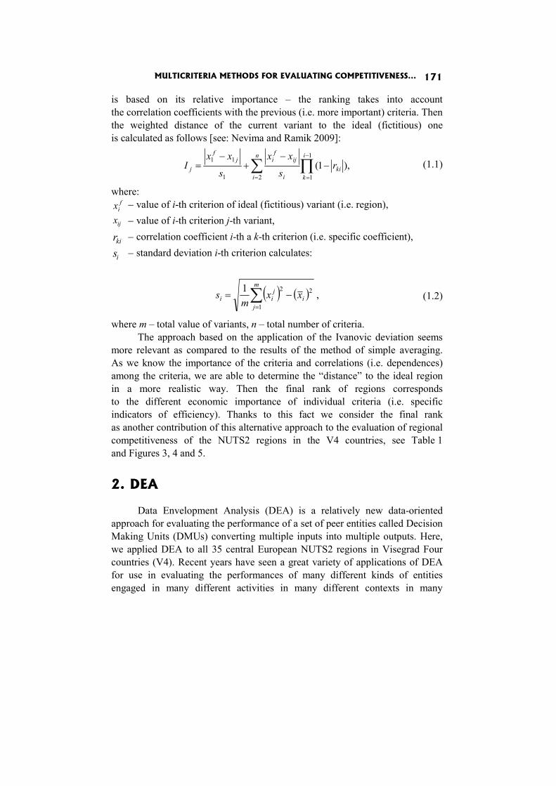
MULTICRITERIA METHODS FOR EVALUATING COMPETITIVENESS... 171
is based on its relative importance – the ranking takes into account the correlation coefficients with the previous (i.e. more important) criteria. Then the weighted distance of the current variant to the ideal (fictitious) one is calculated as follows [see: Nevima and Ramik 2009]:
),1(1
121
11 ∏∑−
==
−−
+−
=i
kki
n
i i
ijf
ijf
j rs
xx
s
xxI (1.1)
where: f
ix − value of i-th criterion of ideal (fictitious) variant (i.e. region),
ijx − value of i-th criterion j-th variant,
kir − correlation coefficient i-th a k-th criterion (i.e. specific coefficient),
is − standard deviation i-th criterion calculates:
( ) ( ) ,1 2
1
2i
m
j
jii xx
ms −= ∑
=
(1.2)
where m – total value of variants, n – total number of criteria. The approach based on the application of the Ivanovic deviation seems
more relevant as compared to the results of the method of simple averaging. As we know the importance of the criteria and correlations (i.e. dependences) among the criteria, we are able to determine the “distance” to the ideal region in a more realistic way. Then the final rank of regions corresponds to the different economic importance of individual criteria (i.e. specific indicators of efficiency). Thanks to this fact we consider the final rank as another contribution of this alternative approach to the evaluation of regional competitiveness of the NUTS2 regions in the V4 countries, see Table 1 and Figures 3, 4 and 5.
2. DEA
Data Envelopment Analysis (DEA) is a relatively new data-oriented approach for evaluating the performance of a set of peer entities called Decision Making Units (DMUs) converting multiple inputs into multiple outputs. Here, we applied DEA to all 35 central European NUTS2 regions in Visegrad Four countries (V4). Recent years have seen a great variety of applications of DEA for use in evaluating the performances of many different kinds of entities engaged in many different activities in many different contexts in many
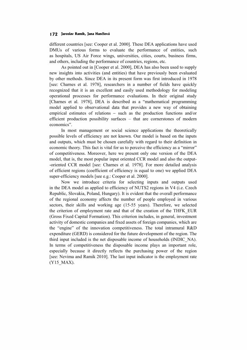
Jaroslav Ramík, Jana Hančlová 172
different countries [see: Cooper et al. 2000]. These DEA applications have used DMUs of various forms to evaluate the performance of entities, such as hospitals, US Air Force wings, universities, cities, courts, business firms, and others, including the performance of countries, regions, etc.
As pointed out in [Cooper et al. 2000], DEA has also been used to supply new insights into activities (and entities) that have previously been evaluated by other methods. Since DEA in its present form was first introduced in 1978 [see: Charnes et al. 1978], researchers in a number of fields have quickly recognized that it is an excellent and easily used methodology for modeling operational processes for performance evaluations. In their original study [Charnes et al. 1978], DEA is described as a “mathematical programming model applied to observational data that provides a new way of obtaining empirical estimates of relations − such as the production functions and/or efficient production possibility surfaces – that are cornerstones of modern economics”.
In most management or social science applications the theoretically possible levels of efficiency are not known. Our model is based on the inputs and outputs, which must be chosen carefully with regard to their definition in economic theory. This fact is vital for us to perceive the efficiency as a “mirror” of competitiveness. Moreover, here we present only one version of the DEA model, that is, the most popular input oriented CCR model and also the output- -oriented CCR model [see: Charnes et al. 1978]. For more detailed analysis of efficient regions (coefficient of efficiency is equal to one) we applied DEA super-efficiency models [see e.g.: Cooper et al. 2000].
Now we introduce criteria for selecting inputs and outputs used in the DEA model as applied to efficiency of NUTS2 regions in V4 (i.e. Czech Republic, Slovakia, Poland, Hungary). It is evident that the overall performance of the regional economy affects the number of people employed in various sectors, their skills and working age (15-55 years). Therefore, we selected the criterion of employment rate and that of the creation of the THFK_EUR (Gross Fixed Capital Formation). This criterion includes, in general, investment activity of domestic companies and fixed assets of foreign companies, which are the “engine” of the innovation competitiveness. The total intramural R&D expenditure (GERD) is considered for the future development of the region. The third input included is the net disposable income of households (INDIC_NA). In terms of competitiveness the disposable income plays an important role, especially because it directly reflects the purchasing power of the region [see: Nevima and Ramik 2010]. The last input indicator is the employment rate (Y15_MAX).
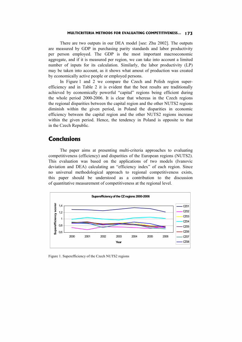
MULTICRITERIA METHODS FOR EVALUATING COMPETITIVENESS... 173
There are two outputs in our DEA model [see: Zhu 2002]. The outputs are measured by GDP in purchasing parity standards and labor productivity per person employed. The GDP is the most important macroeconomic aggregate, and if it is measured per region, we can take into account a limited number of inputs for its calculation. Similarly, the labor productivity (LP) may be taken into account, as it shows what amout of production was created by economically active people or employed persons.
In Figure 1 and 2 we compare the Czech and Polish region super-efficiency and in Table 2 it is evident that the best results are traditionally achieved by economically powerful “capital” regions being efficient during the whole period 2000-2006. It is clear that whereas in the Czech regions the regional disparities between the capital region and the other NUTS2 regions diminish within the given period, in Poland the disparities in economic efficiency between the capital region and the other NUTS2 regions increase within the given period. Hence, the tendency in Poland is opposite to that in the Czech Republic.
Conclusions
The paper aims at presenting multi-criteria approaches to evaluating competitiveness (efficiency) and disparities of the European regions (NUTS2). This evaluation was based on the applications of two models (Ivanovic deviation and DEA) calculating an “efficiency index” of each region. Since no universal methodological approach to regional competitiveness exists, this paper should be understood as a contribution to the discussion of quantitative measurement of competitiveness at the regional level.
Figure 1. Superefficiency of the Czech NUTS2 regions
Superefficiency of the CZ regions 2000-2006
0,6
0,8
1
1,2
1,4
2000 2001 2002 2003 2004 2005 2006
Year
Supe
reff
icie
ncy
scor
en CZ01
CZ02
CZ03
CZ04
CZ05
CZ06
CZ07
CZ08

Jaroslav Ramík, Jana Hančlová 174
Figure 2. Superefficiency of the Polish NUTS2 regions
Figure 3. Ivanovic deviation of the Czech NUTS2 regions
Figure 4. Ivanovic deviation of the Polish NUTS2 regions
0,6
1,1
1,6
2,1
2,6
3,1
2000 2001 2002 2003 2004 2005 2006
Supe
reffic
iency
sco
re
Year
Superefficiency of the PL regions 2000-2006PL11
PL12
PL21
PL22
PL31
PL32
PL33
PL34
PL41
PL42
PL43
PL51
PL52
PL61
PL62
PL63
Ivanovic dev. of the CZ regions 2000-2006
0,000
1,000
2,000
3,000
4,000
5,000
6,000
2000 2001 2002 2003 2004 2005 2006
Year
sco
re
CZ01CZ02CZ03CZ04CZ05CZ06CZ07CZ08
Ivanovic dev. of the PL regions 2000-2006
0,000
1,000
2,000
3,000
4,000
5,000
6,000
2000 2001 2002 2003 2004 2005 2006
Year
sco
re
PL11PL12PL21PL22PL31PL32PL33PL34PL41PL42PL43PL51PL52PL61PL62PL63

MULTICRITERIA METHODS FOR EVALUATING COMPETITIVENESS... 175
Figure 5. Ivanovic deviation of the V4 regions
Ivanovic dev. of the V4 regions 2000-2006
0,000
1,000
2,000
3,000
4,000
5,000
6,000
2000 2001 2002 2003 2004 2005 2006
sco
re
CZ01CZ02CZ03CZ04CZ05CZ06CZ07CZ08HU10HU21HU22HU23HU31HU32HU33PL11PL12PL21PL22PL31PL32PL33PL34PL41PL42PL43PL51PL52PL61PL62PL63SK01SK02SK03SK04
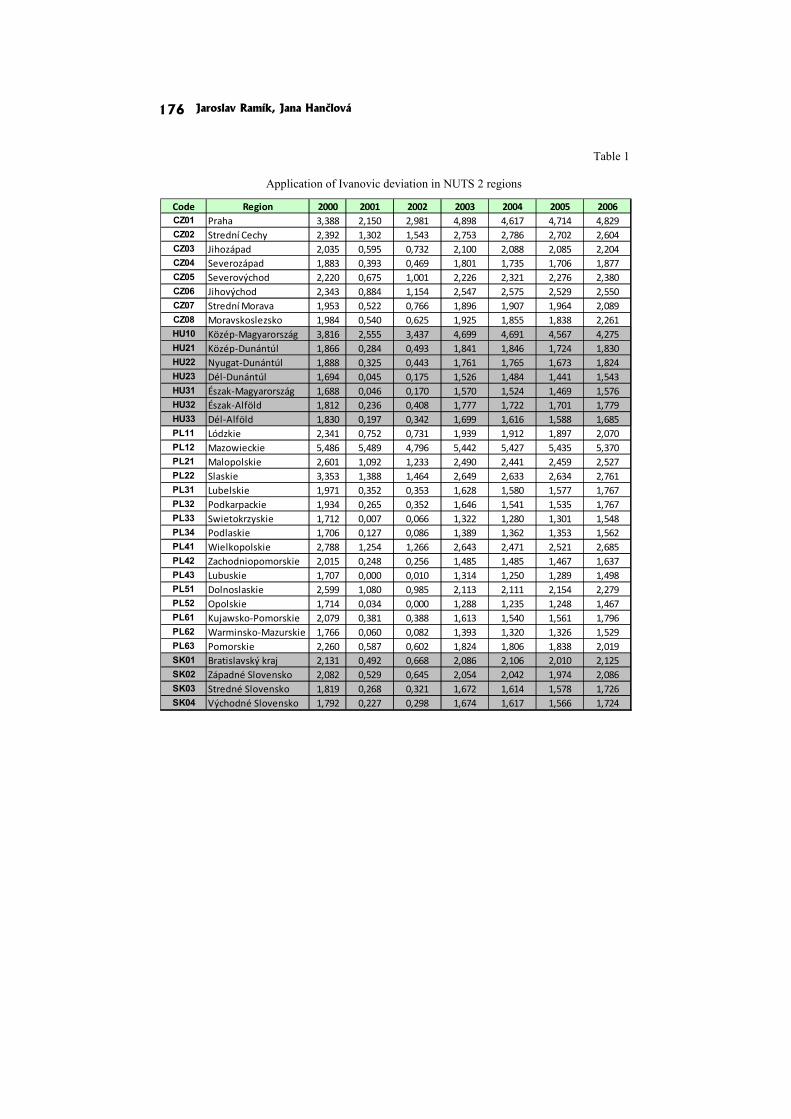
Jaroslav Ramík, Jana Hančlová 176
Table 1
Application of Ivanovic deviation in NUTS 2 regions
Code Region 2000 2001 2002 2003 2004 2005 2006CZ01 Praha 3,388 2,150 2,981 4,898 4,617 4,714 4,829CZ02 Strední Cechy 2,392 1,302 1,543 2,753 2,786 2,702 2,604CZ03 Jihozápad 2,035 0,595 0,732 2,100 2,088 2,085 2,204CZ04 Severozápad 1,883 0,393 0,469 1,801 1,735 1,706 1,877CZ05 Severovýchod 2,220 0,675 1,001 2,226 2,321 2,276 2,380CZ06 Jihovýchod 2,343 0,884 1,154 2,547 2,575 2,529 2,550CZ07 Strední Morava 1,953 0,522 0,766 1,896 1,907 1,964 2,089CZ08 Moravskoslezsko 1,984 0,540 0,625 1,925 1,855 1,838 2,261HU10 Közép-Magyarország 3,816 2,555 3,437 4,699 4,691 4,567 4,275HU21 Közép-Dunántúl 1,866 0,284 0,493 1,841 1,846 1,724 1,830HU22 Nyugat-Dunántúl 1,888 0,325 0,443 1,761 1,765 1,673 1,824HU23 Dél-Dunántúl 1,694 0,045 0,175 1,526 1,484 1,441 1,543HU31 Észak-Magyarország 1,688 0,046 0,170 1,570 1,524 1,469 1,576HU32 Észak-Alföld 1,812 0,236 0,408 1,777 1,722 1,701 1,779HU33 Dél-Alföld 1,830 0,197 0,342 1,699 1,616 1,588 1,685PL11 Lódzkie 2,341 0,752 0,731 1,939 1,912 1,897 2,070PL12 Mazowieckie 5,486 5,489 4,796 5,442 5,427 5,435 5,370PL21 Malopolskie 2,601 1,092 1,233 2,490 2,441 2,459 2,527PL22 Slaskie 3,353 1,388 1,464 2,649 2,633 2,634 2,761PL31 Lubelskie 1,971 0,352 0,353 1,628 1,580 1,577 1,767PL32 Podkarpackie 1,934 0,265 0,352 1,646 1,541 1,535 1,767PL33 Swietokrzyskie 1,712 0,007 0,066 1,322 1,280 1,301 1,548PL34 Podlaskie 1,706 0,127 0,086 1,389 1,362 1,353 1,562PL41 Wielkopolskie 2,788 1,254 1,266 2,643 2,471 2,521 2,685PL42 Zachodniopomorskie 2,015 0,248 0,256 1,485 1,485 1,467 1,637PL43 Lubuskie 1,707 0,000 0,010 1,314 1,250 1,289 1,498PL51 Dolnoslaskie 2,599 1,080 0,985 2,113 2,111 2,154 2,279PL52 Opolskie 1,714 0,034 0,000 1,288 1,235 1,248 1,467PL61 Kujawsko-Pomorskie 2,079 0,381 0,388 1,613 1,540 1,561 1,796PL62 Warminsko-Mazurskie 1,766 0,060 0,082 1,393 1,320 1,326 1,529PL63 Pomorskie 2,260 0,587 0,602 1,824 1,806 1,838 2,019SK01 Bratislavský kraj 2,131 0,492 0,668 2,086 2,106 2,010 2,125SK02 Západné Slovensko 2,082 0,529 0,645 2,054 2,042 1,974 2,086SK03 Stredné Slovensko 1,819 0,268 0,321 1,672 1,614 1,578 1,726SK04 Východné Slovensko 1,792 0,227 0,298 1,674 1,617 1,566 1,724
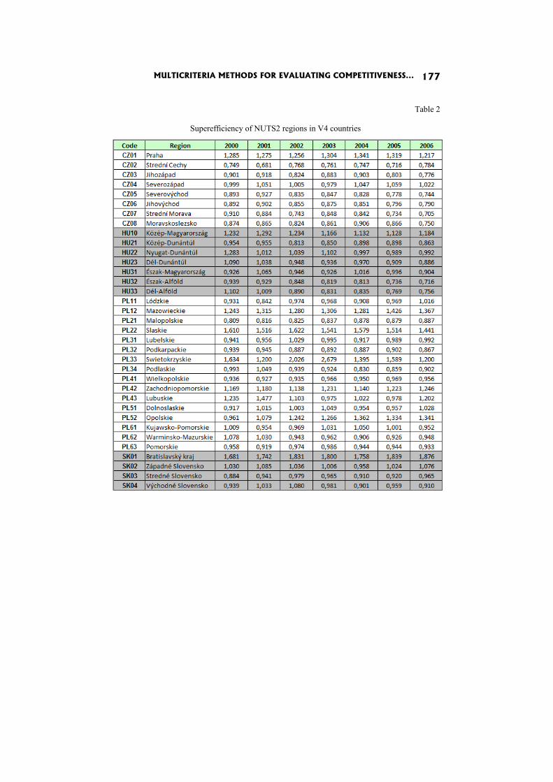
MULTICRITERIA METHODS FOR EVALUATING COMPETITIVENESS... 177
Table 2
Superefficiency of NUTS2 regions in V4 countries

Jaroslav Ramík, Jana Hančlová 178
Acknowledgements
The research work was supported by the Czech Science Foundation, grant number 402/08/1015 − Macroeconomic Models of the Czech Economy and Economies of the other EU Countries.
References
Charnes A., Cooper W., Rhodes E. (1978), Measuring the Efficiency of Decision Making Units, “European Journal of Operational Research”, No. 2.
Cooper W., Seiford L., Tone K. (2000), Data Envelopment Analysis: A Comprehensive Text with Models, Applications, References and DEA-Solver Software, Kluwer Academic Publishers, Boston.
Krugman P. (1994), Competitiveness: A Dangerous Obsession, “Foreign Affairs”, March/April.
Melecký L., Nevima J. (2010), Regionální konkurenceschopnost a možnosti jejího hodnocení v zemích V4 prostřednictvím aplikace specifických ekonomických koeficientů, “Acta Academica Karviniensia”, No. 1.
Nevima J., Ramik J. (2009), Application of Multicriteria Decision Making for Evalu-ation of Regional Competitiveness, in: Mathematical Methods in Economics 2009, Kostelec nad Černými lesy 9.-11.9.2009, Czech University of Life Sciences Prague: Faculty of Economics and Management.
Nevima J., Ramik J. (2010), Application of DEA for Evaluation of Regional Efficiency of EU Regions, in: Mathematical Methods in Economics 2010, České Budějovice 8.-10.9.2010, University of South Bohemia.
Total Economy Database – OECD. Regional statistics. 2010, http://stats.oecd.org /Index.aspx.
Ramík J., Perzina R. (2008), Moderní metody hodnocení a rozhodování. Studia Oeconomica, Slezská univerzita v Opavě, OPF v Karviné.
Zhu J. (2002), Quantitative Models for Performance Evaluation and Benchmarking: Data Envelopment Analysis with Spreadsheets and DEA Excel Solver, Kluwer Academic Publishers, Boston.
Tomas Subrt
Helena Brozova
MULTIPLE CRITERIA EVALUATION OF PROJECT GOALS
Abstract
This text is focussed on the quantitative evaluation of project SMART goals using the ANP method. This approach should be used in the project initiation phase. The very first step in all projects: business, home, or education, is to define goals and objectives. It is important to develop several goals that will enable us to be successful. Goals should be SMART − S − specific, significant, stretching, M − measurable, meaningful, motivational, manageable, A − agreed upon, attainable, achievable, acceptable, action-oriented, R − realistic, relevant, reasonable, rewarding, results-oriented, resourced, T − time-based, timely, tangible, trackable.
In our paper we make complex decisions about satisfying project SMART goals based on the ANP method using Super Decisions Software. As criteria we used a general SMART (SMARTER) model, as sub-criteria we use S, M, A, R, T sub-goals and as alternatives different project schedules are applied. We experiment with their mutual dependencies and we try to propose the best methodology for evaluating projects using the Analytic Network Process.
Keywords
Project management, project proposal, evaluation of project goals achievement, Analytic Network Process, Super Decisions Software.
Introduction
Modern project management uses many methods, techniques and tools for evaluating the quality of a project, both in the phase of proposal and in the phase of realization. Any project proposal should look very nice but a deeper study of its aim, time schedule, and resource allocation can detect whether it is likely to fail/to succeed. The majority of methods used for project evaluation are not based on quantitative approaches; sophisticated mathematical methods of multiple criteria evaluation of alternatives are used only very rarely.
Tomas Subrt, Helena Brozova 180
The BOSCARD (Background, Objectives, Scope, Constraints, Assumptions, Risks and Deliverables) is a tool used to provide the terms-of- -reference for the newly proposed project [Haughey 2011]. It is used in the phase of project initiation. What future events may impact the project? For forecasting the future and customizing the project schedule the Delphi Step by Step technique can help. The MoSCoW method (Must have this, Should have this if at all possible, Could have this if it does not affect anything else, Won't have this time but Would like in the future) is applied when establishing a clear understanding of the customers' requirements and their priorities [Clegg and Barker 2004]. The PEST is a strategic planning tool for evaluating the possible impact of Political, Economic, Social, and Technological factors on a project. The RACI model (Responsibility, Accountability, Consultation, and Information) is a straightforward tool used for identifying roles and respon-sibilities and avoiding confusion over those roles and responsibilities during a project [Smith 2005]. SWOT analysis (Strengths, Weaknesses, Opportunities, Threats) is a well known strategic planning tool used to evaluate the strengths, weaknesses, opportunities, and threats to a project [Armstrong 2006]. It involves specifying the objective of the project and identifying the internal and external factors that are favourable and unfavourable to achieving that objective.
The tool we consider in this paper is called SMART Goals evaluation. Project goals should be SMART [Doran 1981], which very briefly means: S − specific, significant, M − measurable, manageable, A − agreed, action- -oriented, R − realistic, relevant, resourced, T − time-based, trackable. SMARTI project adds I − Integrated criteria to SMART goals, SMARTER project is moreover E − Ethical, Excitable, Enjoyable, Engaging, Ecological and R − Rewarded, Reassess, Revisit, Recordable.
For our paper it is more important to evaluate a completed project, final proposals, or project baselines (schedules) whether the SMART goals have been achieved or not. These goals are hard to measure; they have no final quantitative features. That is why we first tried to apply the Analytic Hierarchy Process [Saaty 1980, 1999] for comparing a finite set of projects with respect to general SMART goals (criteria) and individual SMART specifications (sub-criteria). Upon receiving the AHP results we decided to abandon this approach and apply the Analytic Network Process [Saaty 2001, 2003] for this evaluation. In the AHP each element in the hierarchy is considered to be independent of all the others, the ANP does not require independence among elements. It is very
MULTIPLE CRITERIA EVALUATION OF PROJECT GOALS 181
hard to make complex decision on satisfying project SMART goals without applying the ANP method because SMART specifications (sub-criteria) are not independent of each other. The majority of them are judged from sometimes very various points of views and one judgment strongly influences the others. R – goals (sub-criteria) “Realistic” and “Relevant” are typical examples of this dependency.
According to the survey [White and Fortune 2001] three crucial success factors mentioned most frequently by respondents were: – Clear goals. – Support from senior management. – Adequate funds/resources. That’s why we focus mostly on project goals.
1. The ANP process as a tool for SMART goals evaluation
Multiple criteria decision models are used by many industries to quantify, compare, and manage their performance. The Analytic Network Process is one of the most effective tools in cases where the interactions among qualitative and quantitative factors generate a hierarchical or a network structure. Isik at all [2007] presented a conceptual performance measurement framework that takes into account company-level factors (objectives, strategies, resources) as well as project-level (risks, opportunities) and market-level factors (com-petition, demand).
As a tool for SMART goals achievement evaluation the hierarchy evaluation by the Analytic Network Process (Saaty 2001, 2003) should be used. Two types of the ANP model are theoretically defined: the Feedback System model and the Series System model. The Series System model usually consists of a tree, where the root is a model goal; branches of various levels have the meaning of criteria or sub-criteria of various levels respectively and finally the leaves represent a set of alternatives. Branches and leaves together determine the so-called model clusters (criteria, sub-criteria, project proposals). A crucial role for the project proposal evaluation plays the Feedback System model, where the clusters are linked one by one into a complex network system. We assume that all sub-criteria (within S, M, A, R and T criteria) influence and interact with each other and in the same way all the criteria are inter-connected, too. It means that the hierarchy structure can be transformed into
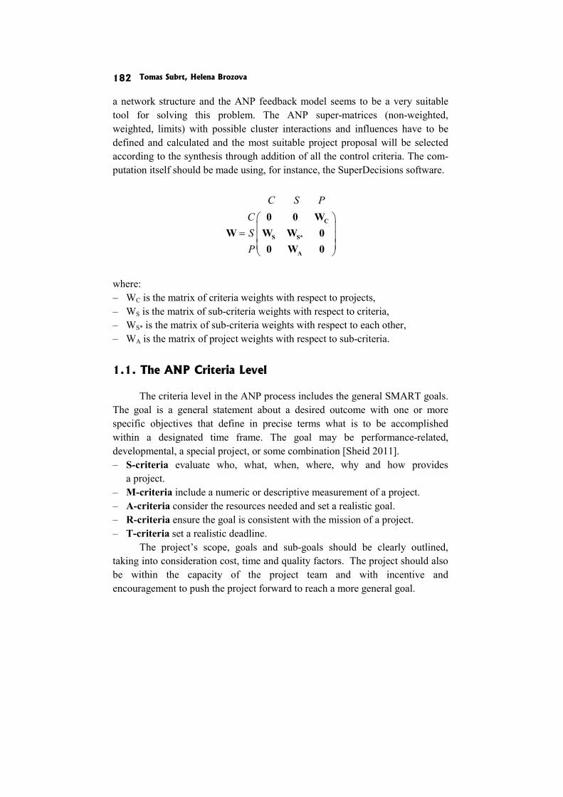
Tomas Subrt, Helena Brozova 182
a network structure and the ANP feedback model seems to be a very suitable tool for solving this problem. The ANP super-matrices (non-weighted, weighted, limits) with possible cluster interactions and influences have to be defined and calculated and the most suitable project proposal will be selected according to the synthesis through addition of all the control criteria. The com-putation itself should be made using, for instance, the SuperDecisions software.
C S PCSP
⎛ ⎞⎜ ⎟= ⎜ ⎟⎜ ⎟⎝ ⎠
C
S S*
A
0 0 WW W W 0
0 W 0
where: – WC is the matrix of criteria weights with respect to projects, – WS is the matrix of sub-criteria weights with respect to criteria, – WS* is the matrix of sub-criteria weights with respect to each other, – WA is the matrix of project weights with respect to sub-criteria.
1.1. The ANP Criteria Level
The criteria level in the ANP process includes the general SMART goals. The goal is a general statement about a desired outcome with one or more specific objectives that define in precise terms what is to be accomplished within a designated time frame. The goal may be performance-related, developmental, a special project, or some combination [Sheid 2011]. – S-criteria evaluate who, what, when, where, why and how provides
a project. – M-criteria include a numeric or descriptive measurement of a project. – A-criteria consider the resources needed and set a realistic goal. – R-criteria ensure the goal is consistent with the mission of a project. – T-criteria set a realistic deadline.
The project’s scope, goals and sub-goals should be clearly outlined, taking into consideration cost, time and quality factors. The project should also be within the capacity of the project team and with incentive and encouragement to push the project forward to reach a more general goal.

MULTIPLE CRITERIA EVALUATION OF PROJECT GOALS 183
1.2. The ANP Sub-criteria Level
Many meanings of the S, M, A, R, T letters are known from the literature. For example, A-criteria should be divided into Actionable, Attainable, Ambitious, Aspirational, Accepted/Acceptable, Aligned, Accountable, Agreed, Adapted, As-if-now, Adjustable, Adaptable etc. [RapidBI 2011].
For the ANP process analysis we have decided to use the following sub-criteria. We don’t aspire to actual project evaluation, our aim is to propose a methodology of using the ANP process in this type of problems. Any other sub-criteria can be set or applied. – Specific − What exactly are we going to do, with or for whom? “Specific”
in the context of developing objectives refers to an observable action, behaviour or achievement.
– Significant − Significant goals are the ones that will make a positive difference in reality.
– Measurable − A method or procedure allowing the tracking and recording the project behaviour or progress must exist.
– Meaningful – Realization of a project must have a meaning. The goal must be very important.
– Manageable − The project must be easy to manage! – Achievable − It must be possible for the project to be done in the
timeframe/in this political climate/with this amount of money. – Action Oriented − The plan of “attack” to make each goal real. – Relevant − The project goal being set with an individual is something that
can impact, change or be important to the organization – Realistic − It must be an objective toward which you are both willing and
able to work. – Resourced − The goal or target being set is something that must have
relevant resources allocated to be satisfied. – Time Based − Every project task must have clearly stated a finish and/or
a start date. – Trackable − All goals should be trackable so you can see what your
progress is. In terms of Project Management, you are tracking progress of project tasks in time, earned value, work etc.
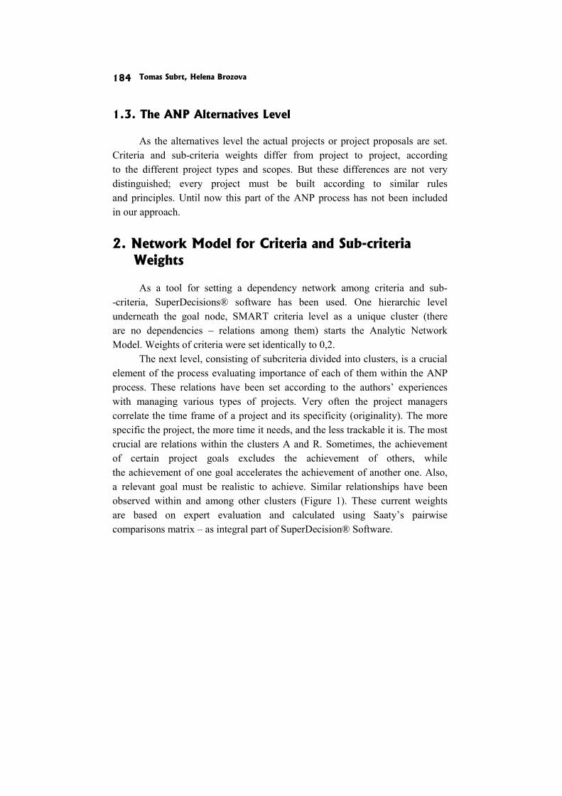
Tomas Subrt, Helena Brozova 184
1.3. The ANP Alternatives Level
As the alternatives level the actual projects or project proposals are set. Criteria and sub-criteria weights differ from project to project, according to the different project types and scopes. But these differences are not very distinguished; every project must be built according to similar rules and principles. Until now this part of the ANP process has not been included in our approach.
2. Network Model for Criteria and Sub-criteria Weights
As a tool for setting a dependency network among criteria and sub- -criteria, SuperDecisions® software has been used. One hierarchic level underneath the goal node, SMART criteria level as a unique cluster (there are no dependencies – relations among them) starts the Analytic Network Model. Weights of criteria were set identically to 0,2.
The next level, consisting of subcriteria divided into clusters, is a crucial element of the process evaluating importance of each of them within the ANP process. These relations have been set according to the authors’ experiences with managing various types of projects. Very often the project managers correlate the time frame of a project and its specificity (originality). The more specific the project, the more time it needs, and the less trackable it is. The most crucial are relations within the clusters A and R. Sometimes, the achievement of certain project goals excludes the achievement of others, while the achievement of one goal accelerates the achievement of another one. Also, a relevant goal must be realistic to achieve. Similar relationships have been observed within and among other clusters (Figure 1). These current weights are based on expert evaluation and calculated using Saaty’s pairwise comparisons matrix – as integral part of SuperDecision® Software.
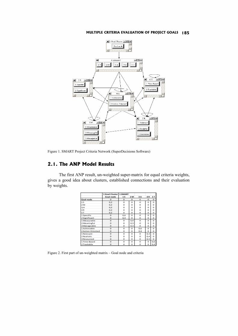
MULTIPLE CRITERIA EVALUATION OF PROJECT GOALS 185
Figure 1. SMART Project Criteria Network (SuperDecisions Software)
2.1. The ANP Model Results
The first ANP result, un-weighted super-matrix for equal criteria weights, gives a good idea about clusters, established connections and their evaluation by weights.
Figure 2. First part of un-weighted matrix – Goal node and criteria
1 Goal Cluster 1 SMARTGoal node 1 S 2 M 3 A 4 R 5 T
Goal node 0 0 0 0 0 01 S 0,2 0 0 0 0 02 M 0,2 0 0 0 0 03,A 0,2 0 0 0 0 04 R 0,2 0 0 0 0 05 T 0,2 0 0 0 0 01 Specific 0 0,6 0 0 0 02 Significant 0 0,4 0 0 0 01 Measurable 0 0 0,4 0 0 02 Meaningful 0 0 0,3 0 0 03 Manageable 0 0 0,3 0 0 01 Achievable 0 0 0 0,6 0 02 Action Oriented 0 0 0 0,4 0 01 Relevant 0 0 0 0 0,3 02 Realistic 0 0 0 0 0,4 03 Resourced 0 0 0 0 0,3 01 Time Based 0 0 0 0 0 0,62 Trackable 0 0 0 0 0 0,4
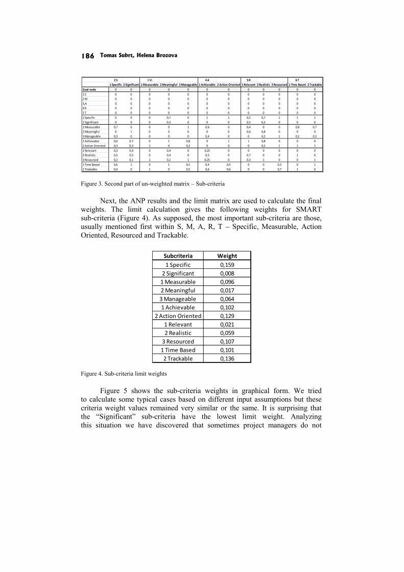
Tomas Subrt, Helena Brozova 186
Figure 3. Second part of un-weighted matrix – Sub-criteria Next, the ANP results and the limit matrix are used to calculate the final
weights. The limit calculation gives the following weights for SMART sub-criteria (Figure 4). As supposed, the most important sub-criteria are those, usually mentioned first within S, M, A, R, T – Specific, Measurable, Action Oriented, Resourced and Trackable.
Figure 4. Sub-criteria limit weights Figure 5 shows the sub-criteria weights in graphical form. We tried
to calculate some typical cases based on different input assumptions but these criteria weight values remained very similar or the same. It is surprising that the “Significant” sub-criteria have the lowest limit weight. Analyzing this situation we have discovered that sometimes project managers do not
2 S 3 M 4 A 5 R 6 T1 Specific 2 Significant 1 Measurable 2 Meaningful 3 Manageable 1 Achievable 2 Action Oriented 1 Relevant 2 Realistic 3 Resourced 1 Time Based 2 Trackable
Goal node 0 0 0 0 0 0 0 0 0 0 0 01 S 0 0 0 0 0 0 0 0 0 0 0 02 M 0 0 0 0 0 0 0 0 0 0 0 03,A 0 0 0 0 0 0 0 0 0 0 0 04 R 0 0 0 0 0 0 0 0 0 0 0 05 T 0 0 0 0 0 0 0 0 0 0 0 01 Specific 0 0 0 0,7 0 1 1 0,5 0,7 1 1 12 Significant 0 0 0 0,3 0 0 0 0,5 0,3 0 0 01 Measurable 0,7 0 0 0 1 0,6 0 0,4 0 0 0,8 0,72 Meaningful 0 1 0 0 0 0 0 0,6 0,8 0 0 03 Manageable 0,3 0 0 0 0 0,4 0 0 0,2 1 0,2 0,31 Achievable 0,6 0,7 0 1 0,8 0 1 1 0,8 0 0 02 Action Oriented 0,4 0,3 1 0 0,2 0 0 0 0,2 1 1 11 Relevant 0,3 0,4 0 0,4 0 0,25 0 0 0 0 0 02 Realistic 0,5 0,5 0 0,4 0 0,5 0 0,7 0 0 1 03 Resourced 0,2 0,1 1 0,2 1 0,25 0 0,3 1 0 0 11 Time Based 0,6 1 0 1 0,5 0,4 0,4 0 0 0,3 0 12 Trackable 0,4 0 1 0 0,5 0,6 0,6 0 0 0,7 1 0
Subcriteria Weight1 Specific 0,159
2 Significant 0,0081 Measurable 0,0962 Meaningful 0,0173 Manageable 0,0641 Achievable 0,102
2 Action Oriented 0,1291 Relevant 0,0212 Realistic 0,059
3 Resourced 0,1071 Time Based 0,1012 Trackable 0,136

MULTIPLE CRITERIA EVALUATION OF PROJECT GOALS 187
understand what the expressions “Significant project, significant goal” mean. Often, they assume that every project is significant and therefore they have unrealistic expectations with regard to the values of this sub-criteria weight.
Figure 5. Sub-criteria limit weights − chart view
Conclusions
The aim of the paper was to analyse quality and quantity of various criteria frequently used while evaluating a project within a project management process. We have chosen the SMART approach to evaluate the fulfilment of project goals. – The methodology used seems to be useful for the analysis of various projects
according to more or less differing criteria. – The ANP method allows description and research of complex dependencies
among the important project criteria from various points of view. Network dependencies are typical for this problem.
– Our future research will be focused on criteria weights and on actual project proposal assessment. These weights have to be estimated by experts’ judgement, because the set of SMART criteria requires the soft system approach.
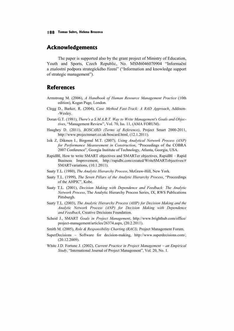
Tomas Subrt, Helena Brozova 188
Acknowledgements
The paper is supported also by the grant project of Ministry of Education, Youth and Sports, Czech Republic, No. MSM6046070904 “Informační a znalostní podpora strategického řízení” (“Information and knowledge support of strategic management”).
References
Armstrong M. (2006), A Handbook of Human Resource Management Practice (10th edition), Kogan Page, London.
Clegg D., Barker, R. (2004), Case Method Fast-Track: A RAD Approach, Addison- -Wesley.
Doran G.T. (1981), There's a S.M.A.R.T. Way to Write Management's Goals and Objec-tives, “Management Review”, Vol. 70, Iss. 11, (AMA FORUM).
Haughey D. (2011), BOSCARD (Terms of Reference), Project Smart 2000-2011, http://www.projectsmart.co.uk/boscard.html, (12.1.2011).
Isik Z, Dikmen I., Birgonul M.T. (2007), Using Analytical Network Process (ANP) for Performance Measurement in Construction, “Proceedings of the COBRA 2007 Conference”, Georgia Institute of Technology, Atlanta, Georgia, USA.
RapidBI, How to write SMART objectives and SMARTer objectives, RapidBI – Rapid Business Improvement, http://rapidbi.com/created/WriteSMARTobjectives/# SMARTvariations, (10.1.2011).
Saaty T.L. (1980), The Analytic Hierarchy Process, McGraw-Hill, New York. Saaty T.L. (1999), The Seven Pillars of the Analytic Hierarchy Process, “Proceedings
of the AHPIC”, Kobe. Saaty T.L. (2001), Decision Making with Dependence and Feedback: The Analytic
Network Process, The Analytic Hierarchy Process Series, IX, RWS Publications Pittsburgh.
Saaty T.L. (2003), The Analytic Hierarchy Process (AHP) for Decision Making and the Analytic Network Process (ANP) for Decision Making with Dependence and Feedback, Creative Decisions Foundation.
Scheid J., SMART Goals in Project Management, http://www.brighthub.com/office/ project-management/articles/26374.aspx, (20.2.2011).
Smith M. (2005), Role & Responsibility Charting (RACI), Project Management Forum. SuperDecisions − Software for decision-making, http://www.superdecisions.com/,
(20.12.2009). White J.D. Fortune J. (2002), Current Practice in Project Management − an Empirical
Study, “International Journal of Project Management”, Vol. 20, No. 1.
Krzysztof Targiel
Tadeusz Trzaskalik
Małgorzata Trzaskalik-Wyrwa
Gwo Hsiung Tzeng
DEMATEL, ANP AND VICOR BASED HYBRID METHOD APPLICATION TO RESTORATION OF HISTORICAL ORGANS
Abstract
The aim of the paper is to perform ex-post analysis for of a portable organ restoration applying a hybrid method, which combines DEMATEL, ANP and VICOR multicriteria approaches. The analysis of results and comparison with the earlier research based in the scheme of ELECTRE I method is included.
Keywords
Portable organ reconstruction, hybrid multicriteria method, DEMATEL, ANP, VICOR.
Introduction
The goal of the paper [Trzaskalik-Wyrwa et al. 2006] was to determine the best way of renovation of a historic positive organ, found several years ago in the Podlasie region (part of Poland). Portable organs were very popular musical instrument in Poland in the seventeenth and eighteenth centuries. Its popularity was due above all to the ease of handling and possibility of easy transportation. Unfortunately, only several copies of this once so common instrument are nowadays extant in Poland.
The following decision problem arose: what is the best way to reconstruct the found instrument, taking into account a variety of criteria. In [Trzaskalik- -Wyrwa et al. 2006], this issue has been presented as a multi-criteria decision- -making problem and solved by means of ELECTRE I method. Reconstruction of the instrument was performed using the received. recommendation.
Krzysztof Targiel, Tadeusz Trzaskalik, Małgorzata Trzaskalik-Wyrwa, Gwo Hsiung Tzeng 190
ELECTRE I method requires the decision maker to specify criteria weights and subsequent variant ratings. However, interactions among criteria are not analyzed. This possibility can be found in ANP method. Anyway, applying ANP in the source version is numerically troublesome. This is why a hybrid method which combines elements of three multicriteria approaches: DEMATEL [Fontela and Gabus 1974], ANP [Saaty 1999] and VIKOR [Opricovic and Tzeng 2007], allows to overcome numerical difficulties, emerging when performing the calculations using only the ANP method. A description of that hybrid method can be found in [Liu et al. 2012; Tzeng et al. 2007; Tzeng and Huang 2011]. This method is also presented in our paper.
The aim of the research is to perform ex-post analysis for the rediscovered instrument reconstruction by applying hybrid method mentioned above. We want to find out, how to take into account the mutual influence of criteria and whether these mutual influences will affect the selection of the final solution.
The paper is divided into four parts. In chapter 1, we present brief considerations of the decision-making problem, fully described in [Trzaskalik- -Wyrwa et al. 2006]. The criteria considered and the decision variants are described. The second chapter includes a description of the hybrid method, wchich combines elements of DEMATEL, ANP, and VICOR. The third chapter presents the data provided by the expert (co-author of this paper − Małgorzata Trzaskalik-Wyrwa). Some of them (the evaluation of alternatives due to subsequent criteria) were used previously [Trzaskalik-Wyrwa et al. 2006], others (the specification of the mutual influence of criteria) have been prepared by the expert for the purposes of this study. An application of the hybrid method and detais of numerical calculations are presented. The fourth chapter contains an analysis of the results and compare them with the earlier results, obtained in [Trzaskalik-Wyrwa et al. 2006] by means of ELECRE I method.
1. Restoration of historical portable organ as a multicriteria decision process
1.1. Decision criteria
We consider a division of the values of historical organs into four groups: historic, artistic, musical and utilitarian values. We will describe the values constituting each of the four groups [Trzaskalik-Wyrwa et al. 2006].
Historic values determine the character of the object as a document and its influence on the development of historical knowledge. Among the values of this group are scientific values, due to the fact that an organ
DEMATEL, ANP AND VICOR BASED HYBRID METHOD APPLICATION... 191
is an historic object, requiring a scholarly description. Also in this group are technical values, determining the ingenuity of the construction, the quality of the workmanship and the scientific value of its current condition. Also historic emotional values, perceived not only by scientists and scholars, but also by the public at large, belong here.
The ownership values, i. e., values stemming from the ownership of the original item (without hypothetical additions) are connected with honest approach of the conservators to the historic object, in which that what is preserved should be emphasised above all, as opposed to that what we think might have been there.
The group of artistic values is related to the perception of historic organs as works of art, and this is connected with the instrument’s case. To this group belong historic-artistic values, determining whether the solutions chosen by the builders are typical or atypical as well as the importance of the original, its copy or its hypothetical reconstruction. Artistic qualities affect the public independently of the current fashion or style. The artistic effect of the case of historic organ should match musical impressions received by the audience from the musical compositions heard by it.
Musical values become apparent during a musical performance. We deal here with the issue of style (historical musical value) and of sound (musical quality). All of them taken together may reinforce the musical influence on the amateur listener. It can happen that the regaining of musical value and the preservation of the original technical solutions are conflicting goals. In such case we face the problem of utilitarian values of the historic instrument. The notions of live organ and dead organ are related to this group of values. A musically dead organ is an instrument that nowadays cannot fulfil its function of a musical instrument. A live instrument is an instrument capable of being used in musical performance, affecting the audience in various ways. Like any historic object, an organ as a piece of furniture can be also visually dead − not suitable for being exhibited, or else visually alive (independently of its musical “vitality”) − beautiful, but unplayable.
1.2. Decision alternatives
On the basis of research and evaluation of the condition of the individual parts of the instrument (or their lack) 12 renovation treatments of the rediscovered instrument have been suggested. They are decision alternatives, described below [Trzaskalik-Wyrwa et al. 2006].
Krzysztof Targiel, Tadeusz Trzaskalik, Małgorzata Trzaskalik-Wyrwa, Gwo Hsiung Tzeng 192
Alternative A1 Preservation of the instrument as a non-functional, visually unattractive object (“destrukt”) and its exhibition in the form of a group of museum exhibits.
Alternative A2 Integration of the elements of the instrument using racks necessary to place the individual elements in proper places.
Alternative A3 Integration of the parts of the instrument with full completion of the construction elements of the case (without covering the “windows” with reconstructed wood carved ornaments) according to their former shape as concluded from the elements preserved; completion of the missing parts of the mechanism. The pipes remain secured, but do not play.
Alternative A4 Integration of the parts of the instrument with full completion of the construction elements of the case according to their former shape, as concluded from the elements preserved; completion of the missing parts of the mechanism. Reconstruction of the polychrome and covering of the “windows” by a neutral filling (canvas, wooden grill). The pipes remain secured, but do not play.
Alternative A5 Integration of the parts of the instrument with full completion of the construction elements of the case according to their former shape, as concluded from the elements preserved; completion of the missing parts of the mechanism. Reconstruction of the polychrome. Hypothetical reconstruction of the wood carved ornaments filling out the “windows” (on the basis of comparative analysis − it is impossible to achieve the historical truth). The pipes remain secured, but do not play.
Alternative A6 Integration of the parts of the instrument with full completion of the construction elements of the case (without covering the “windows” by reconstructed wood carved ornaments) according to their former shape, as concluded from the elements preserved; completion of the missing parts of the mechanism. Bringing the extant pipes to working condition and reconstruction of the missing pipes, so as to match the sound capabilities of the extant pipes.
Alternative A7 Integration of the parts of the instrument with full completion of the construction elements of the case (without covering the “windows” by reconstructed wood carved ornaments) according to their former shape,
DEMATEL, ANP AND VICOR BASED HYBRID METHOD APPLICATION... 193
as concluded from the elements preserved; completion of the missing parts of the mechanism. Exhibition of the extant historic pipes in a display case without giving them their former technical functionality. Reconstruction of the entire sound system according to preserved models.
Alternative A8 Integration of the parts of the instrument with full completion of the construction elements of the case according to their former shape, as concluded from the elements preserved; completion of the missing parts of the mechanism. Reconstruction of the polychrome and covering the “windows” by a neutral filling (canvas, wooden grill). Bringing the pipes to a working condition and reconstruction of the missing pipes, so as to match the sound capabilities of the extant pipes.
Alternative A9 Integration of the parts of the instrument with full completion of the construction elements of the case according to their former shape, as concluded from the elements preserved; completion of the missing parts of the mechanism. Reconstruction of the polychrome and covering the “windows” by a neutral filling (canvas, wooden grill). Exposition of the extant historical pipes in a display case without bringing them to a working condition. Reconstruction of the whole sound system according to preserved models.
Alternative A10 Integration of the parts of the instrument with full completion of the construction elements of the case according to their former shape, as concluded from the elements preserved and completion of the missing parts of the mechanism. Reconstruction of the polychrome. Hypothetical reconstruction of the wood carved ornaments filling out the “windows” (on the basis of comparative analysis − it is impossible to achieve historical truth). Bringing the pipes to a working condition and reconstruction of the missing pipes so as to match the sound of the sound capabilities of the preserved pipes.
Alternative A11 Integration of the parts of the instrument with full completion of the construction elements of the case according to their former shape, as concluded from the elements preserved and completion of the missing parts of the mechanism. Reconstruction of the polychrome. Hypothetical reconstruction of the wood carved ornaments filling out the “windows” (on the basis of comparative analysis − it is impossible to achieve historical truth). Exhibition of the preserved historic pipes in a display case without bringing them to a working condition. Reconstruction of the whole sound system according to preserved models.
Krzysztof Targiel, Tadeusz Trzaskalik, Małgorzata Trzaskalik-Wyrwa, Gwo Hsiung Tzeng 194
Alternative A12 Preservation of the instrument in its non-functional, visually unattractive condition (as a “destrukt”). Making of an accurate copy. The evaluation focuses on the values of the copy, which is presented to the public.
2. The hybrid method
The hybrid method [Liu et al. 2012; Tzeng et al. 2007; Tzeng and Huang 2011] is a combination of: – DEMATEL – applied to clarify relation between components, – ANP – applied to determine the relationship between the criteria (in limited
supermatrix), – VIKOR – applied to obtain the index values in gaps.
Let A be a finite set of decision alternatives:
A = { A1, A2, …, Al }
C − a set of criteria, divided into n categories (called here aspects, dimensions,clusters):
C = { C1, C2, …, Cn }
where:
{ } nicccCiimiii ,,,,,, 21 KK 1== − is a subset of criteria in i-th aspect
and F – matrix of values of the j-th alternative in the k-th criterion:
F = [ fkj ] , j = 1, 2, …, l, k = 1, 2, …, M
where ∑=
=n
iimM
1
We assume that the criteria are defined so that a higher the value of the criterion is preferred to a lower one. Each criterion is assigned a positive number which reflects the valid contribution of that criteria.
The considered method is divided into following steps:
Step 1: Develop the structure of the problem. The problem is broken down to a level structure.
Step 2: Develop the total influence matrix. Based on the DEMATEL method, interactions between the aspects are explained to construct the map of the direct impact. This step is divided into three sub-steps:
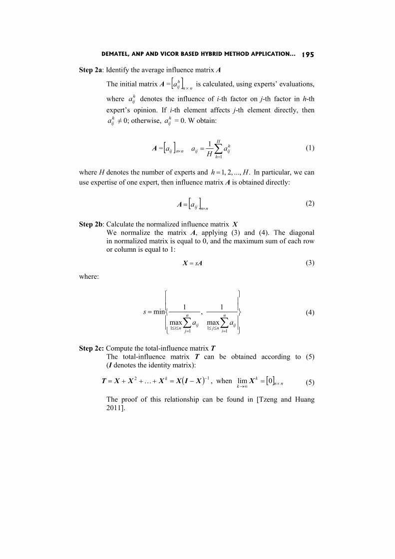
DEMATEL, ANP AND VICOR BASED HYBRID METHOD APPLICATION... 195
Step 2a: Identify the average influence matrix A
The initial matrix A = [ ]nn
hija
× is calculated, using experts’ evaluations,
where hija denotes the influence of i-th factor on j-th factor in h-th
expert’s opinion. If i-th element affects j-th element directly, then hija ≠ 0; otherwise, h
ija = 0. W obtain:
A = [ ] ∑=
× =H
h
hijijnnij a
Haa
1
1 (1)
where H denotes the number of experts and ....,,2,1 Hh = In particular, we can use expertise of one expert, then influence matrix A is obtained directly:
[ ]nnija
×=A (2)
Step 2b: Calculate the normalized influence matrix X We normalize the matrix A, applying (3) and (4). The diagonal in normalized matrix is equal to 0, and the maximum sum of each row or column is equal to 1:
s=X A (3)
where:
⎪⎪
⎭
⎪⎪
⎬
⎫
⎪⎪
⎩
⎪⎪
⎨
⎧
=
∑∑=
≤≤=
≤≤
n
iijnj
n
jijni
aas
1111max
1,max
1min (4)
Step 2c: Compute the total-influence matrix T The total-influence matrix T can be obtained according to (5) (I denotes the identity matrix):
( ) 12 −−=+++= XIXXXXT kK , when [ ] nnk
k ×∞→
= 0lim X (5)
The proof of this relationship can be found in [Tzeng and Huang 2011].

Krzysztof Targiel, Tadeusz Trzaskalik, Małgorzata Trzaskalik-Wyrwa, Gwo Hsiung Tzeng 196
Step 2d: Set a threshold value α and obtain the normalized α-cut total- -influence matrix Tα
We have total-influence matrix T in the form:
⎥⎥⎥⎥⎥⎥
⎦
⎤
⎢⎢⎢⎢⎢⎢
⎣
⎡
=
nnnjn
iniji
nj
ttt
ttt
ttt
KK
MMM
KK
MMM
KK
1
1
1111
T (6)
The α-cut total-influence matrix Tα will be given by Eq. (7)
⎥⎥⎥⎥⎥⎥
⎦
⎤
⎢⎢⎢⎢⎢⎢
⎣
⎡
=
ααα
ααα
ααα
α
nnnjn
iniji
nj
ttt
ttt
ttt
KK
MMM
KK
MMM
KK
1
1
1111
T (7)
where if α<ijt then 0=αijt else ijij tt =α
The α-cut total-influence matrix Tα needs to be normalized by dividing by the value:
nitdn
jiji ,,2,1,
1
K== ∑=
α (8)
Finally we obtain TD as follow:
⎥⎥⎥⎥⎥⎥
⎦
⎤
⎢⎢⎢⎢⎢⎢
⎣
⎡
=
⎥⎥⎥⎥⎥⎥
⎦
⎤
⎢⎢⎢⎢⎢⎢
⎣
⎡
=
Dnn
Dnj
Dn
Din
Dij
Di
Dn
Dj
D
nnnnnjnn
iiniijii
nj
D
ttt
ttt
ttt
dtdtdt
dtdtdt
dtdtdt
KK
MMM
KK
MMM
KK
KK
MMM
KK
MMM
KK
1
1
1111
1
1
1111111
///
///
///
ααα
ααα
ααα
T (9)
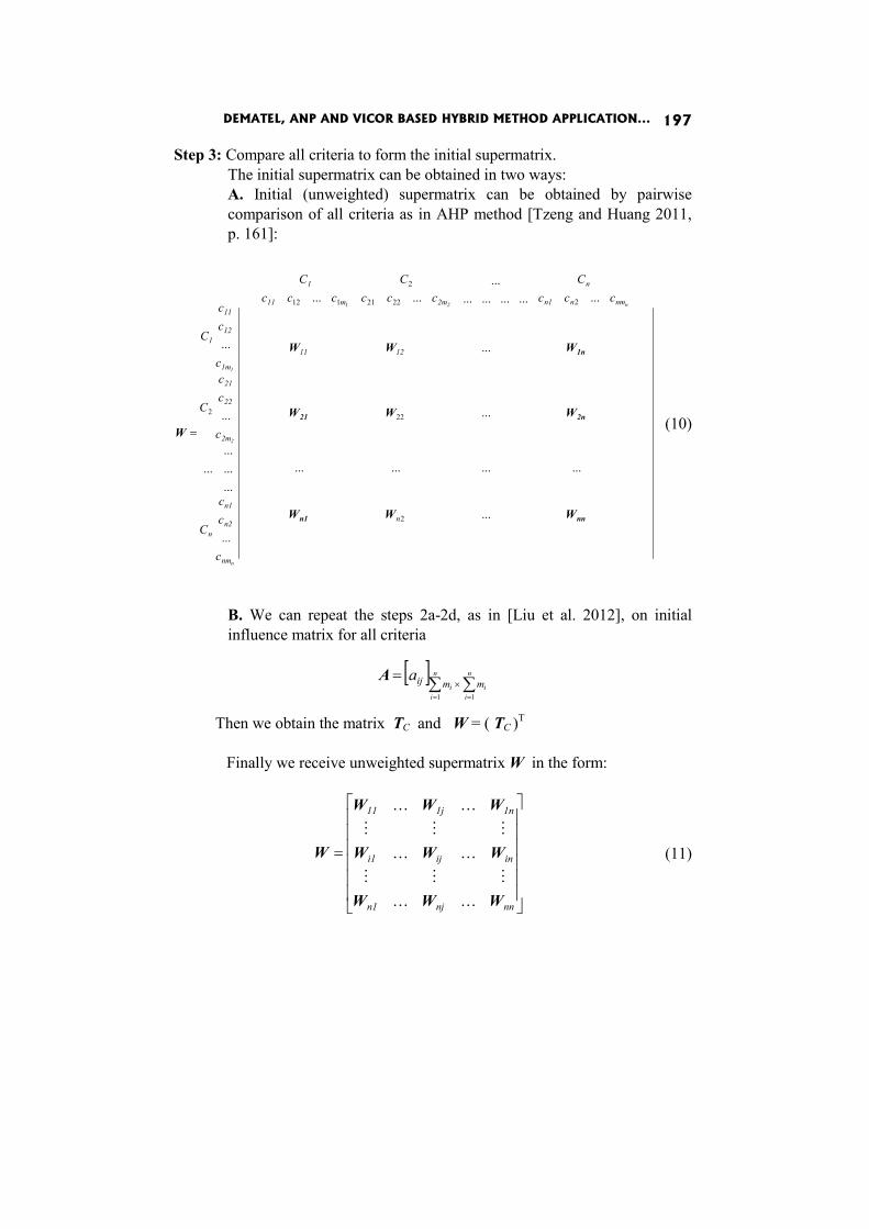
DEMATEL, ANP AND VICOR BASED HYBRID METHOD APPLICATION... 197
Step 3: Compare all criteria to form the initial supermatrix. The initial supermatrix can be obtained in two ways: A. Initial (unweighted) supermatrix can be obtained by pairwise comparison of all criteria as in AHP method [Tzeng and Huang 2011, p. 161]:
nnn1
2n21
1n
WWW
WWW
WWW
W
...
......
...
......
...
..................
......
...
...
......
...
2
22
22221
2
112
2
1
n
11
nm
n
cccC
cccC
cccC
C
C
c
cc
C12
nmn1
n
2m11
1
nm
n2
n1
2m
22
21
1m
12
11
1
n2
n
2
1
c...
cc
c...
cc
=
(10)
B. We can repeat the steps 2a-2d, as in [Liu et al. 2012], on initial influence matrix for all criteria
[ ] ∑∑==
×= n
ii
n
ii mmija
11
A
Then we obtain the matrix TC and W = ( TC )T
Finally we receive unweighted supermatrix W in the form:
⎥⎥⎥⎥⎥⎥
⎦
⎤
⎢⎢⎢⎢⎢⎢
⎣
⎡
=
nnnjn1
iniji1
1n1j11
WWW
WWW
WWW
W
KK
MMM
KK
MMM
KK
(11)

Krzysztof Targiel, Tadeusz Trzaskalik, Małgorzata Trzaskalik-Wyrwa, Gwo Hsiung Tzeng 198
Step 4: Obtain the weighted supermatrix. The normalized TD is multiplied by unweighted supermatrix W to obtain weighted supermatrix Wα. The results are shown in Eq. (12).
⎥⎥⎥⎥⎥⎥
⎦
⎤
⎢⎢⎢⎢⎢⎢
⎣
⎡
×××
×××
×××
=×=
nnnj
inij
1n1j
α
WWW
WWW
WWW
WTW
Dnn
Dnj
Dn1
Din
Diji1
Di1
D1n
Di111
D11
D
ttt
ttt
ttt
KK
MMM
KK
MMM
KK
n1
(12)
Step 5: Obtain the limit supermatrix. The ANP weights of each criterion can be obtained from limit supermatrix:
( )kα
k
lim lim WW∞→
= (13)
The evaluation of the total preference is performed by means of VIKOR method, which can be divided into following steps:
Step 6: Check the best value *
kf and the worse value −kf .
*kf represents the positive-ideal point, that means the expert gives
the scores of the best value (aspired levels) for each criterion and −kf
represents the negative-ideal point, that means the expert gives the scores of the worst values for each criterion. Those values can be computed by the traditional approach, using Eqs. (14) and (15) to obtain the results:
kiik ff max* = , l,K,, 21i = (14)
kiik ff min=− , li ,,, K21= (15)
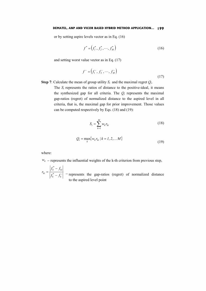
DEMATEL, ANP AND VICOR BASED HYBRID METHOD APPLICATION... 199
or by setting aspire levels vector as in Eq. (16)
( )*M
*2
*1 fff ,,, L=*f (16)
and setting worst value vector as in Eq. (17)
( )−−−− = Mffff ,,, 21 L (17)
Step 7: Calculate the mean of group utility Si and the maximal regret Qi. The Si represents the ratios of distance to the positive-ideal, it means the synthesized gap for all criteria. The Qi represents the maximal gap-ratios (regret) of normalized distance to the aspired level in all criteria, that is, the maximal gap for prior improvement. Those values can be computed respectively by Eqs. (18) and (19):
∑=
=M
kkiki rwS
1
(18)
{ }MkrwQ kikki K,, 21== |max (19)
where:
kw − represents the influential weights of the k-th criterion from previous step,
−−
−=
kk
kikki ff
ffr
*
*
− represents the gap-ratios (regret) of normalized distanceto the aspired level point
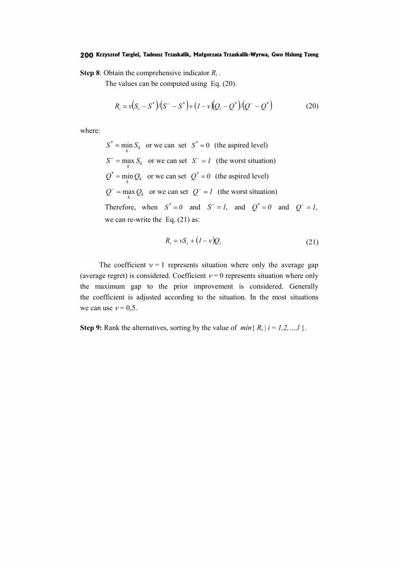
Krzysztof Targiel, Tadeusz Trzaskalik, Małgorzata Trzaskalik-Wyrwa, Gwo Hsiung Tzeng 200
Step 8: Obtain the comprehensive indicator Ri . The values can be computed using Eq. (20).
( ) ( ) ( )( ) ( )**** // QQQQvSSSSvR iii −−−+−−= −− 1 (20)
where:
kkSS min* = or we can set 0* =S (the aspired level)
kkSS max=−
or we can set 1=−S (the worst situation)
kkQQ min* = or we can set 0=*Q (the aspired level)
kkQQ max=−
or we can set 1=−Q (the worst situation)
Therefore, when 0=*S and ,1=−S and 0=*Q and ,1=−Q
we can re-write the Eq. (21) as:
( ) iii QvvSR −+= 1 (21)
The coefficient ν = 1 represents situation where only the average gap (average regret) is considered. Coefficient ν = 0 represents situation where only the maximum gap to the prior improvement is considered. Generally the coefficient is adjusted according to the situation. In the most situations we can use ν = 0,5.
Step 9: Rank the alternatives, sorting by the value of min{ Ri | i = 1,2,…,l }.
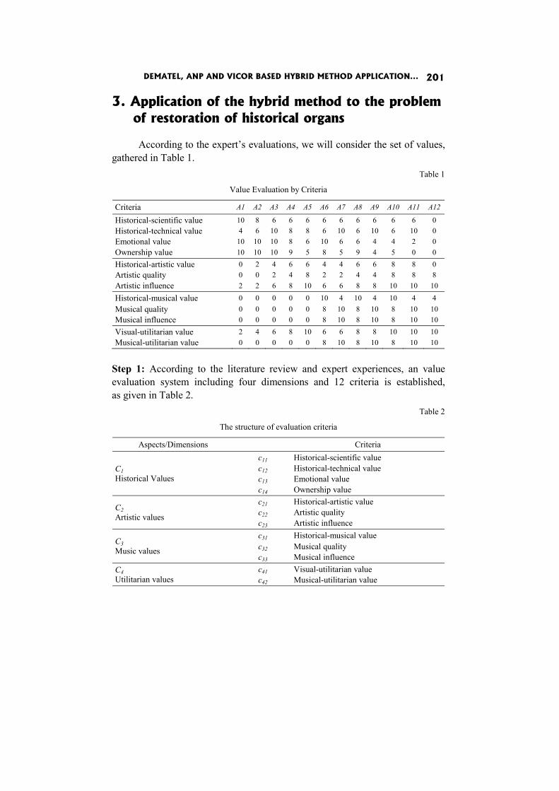
DEMATEL, ANP AND VICOR BASED HYBRID METHOD APPLICATION... 201
3. Application of the hybrid method to the problem of restoration of historical organs
According to the expert’s evaluations, we will consider the set of values, gathered in Table 1.
Table 1
Value Evaluation by Criteria
Criteria A1 A2 A3 A4 A5 A6 A7 A8 A9 A10 A11 A12
Historical-scientific value 10 8 6 6 6 6 6 6 6 6 6 0 Historical-technical value 4 6 10 8 8 6 10 6 10 6 10 0 Emotional value 10 10 10 8 6 10 6 6 4 4 2 0 Ownership value 10 10 10 9 5 8 5 9 4 5 0 0 Historical-artistic value 0 2 4 6 6 4 4 6 6 8 8 0 Artistic quality 0 0 2 4 8 2 2 4 4 8 8 8 Artistic influence 2 2 6 8 10 6 6 8 8 10 10 10
Historical-musical value 0 0 0 0 0 10 4 10 4 10 4 4 Musical quality 0 0 0 0 0 8 10 8 10 8 10 10 Musical influence 0 0 0 0 0 8 10 8 10 8 10 10
Visual-utilitarian value 2 4 6 8 10 6 6 8 8 10 10 10 Musical-utilitarian value 0 0 0 0 0 8 10 8 10 8 10 10
Step 1: According to the literature review and expert experiences, an value evaluation system including four dimensions and 12 criteria is established, as given in Table 2.
Table 2
The structure of evaluation criteria
Aspects/Dimensions Criteria
C1 Historical Values
c11 Historical-scientific value c12 Historical-technical value c13 Emotional value c14 Ownership value
C2 Artistic values
c21 Historical-artistic value c22 Artistic quality c23 Artistic influence
C3 Music values
c31 Historical-musical value c32 Musical quality c33 Musical influence
C4 Utilitarian values
c41 Visual-utilitarian value c42 Musical-utilitarian value

Krzysztof Targiel, Tadeusz Trzaskalik, Małgorzata Trzaskalik-Wyrwa, Gwo Hsiung Tzeng 202
Step 2: The ratings for each criterion’s relationship to sustainable development using a five-point scale ranging from 0 (no effect) to 4 (extremely influential) were collected.
Table 3
Influence between aspects
C1 C2 C3 C4 Historical Values C1 x 2 2 3
Artistic values C2 3 x 0 3 Music values C3 3 0 x 2
Utilitarian values C4 0 4 4 x
Step 2a: Identify the average influence matrix A As it was difficult to the decision maker to determine the influence between aspects themselves, we calculated the influence as rounded average of all influences between the criteria in the aspects. The result is presented in Table 4.
Table 4
Influence matrix
C1 C2 C3 C4 Historical Values C1 2 2 2 3
Artistic values C2 3 2 0 3 Music values C3 3 0 3 2
Utilitarian values C4 0 4 4 0
Step 2b-2d: Total-influential dimensions matrix .DT We used α = 0,1 so it was necessary to normalize the resulting matrix.
Result is presented in Table 5.
Table 5
Total-influential aspects (dimensions) matrix .DT
C1 C2 C3 C4 C1 0,00 0,41 0,28 0,31 C2 0,32 0,00 0,32 0,36 C3 0,28 0,41 0,00 0,31 C4 0,29 0,43 0,29 0,00

DEMATEL, ANP AND VICOR BASED HYBRID METHOD APPLICATION... 203
Step 3: Compare all the criteria to form the initial supermatrix. Because only direct impacts of the criteria were available, we use method B, repeating steps 2a-2d to the matrix presented in Table 6.
Table 6
Influential matrix A on criteria
c11 c12 c13 c14 c21 c22 c23 c31 c32 c33 c41 c42
c11 0 3 1 4 4 4 1 4 1 1 2 2
c12 3 0 1 4 2 1 0 2 1 1 2 2
c13 2 2 0 3 2 2 1 2 1 2 4 4
c14 4 4 4 0 4 4 4 4 4 4 3 3
c21 3 3 3 4 0 4 4 2 2 2 4 0
c22 2 2 2 2 3 0 2 0 0 0 4 0
c23 1 1 1 4 4 4 0 0 0 0 4 0
c31 3 3 2 4 0 0 0 0 4 4 0 4
c32 1 1 0 2 0 0 0 4 0 4 0 4
c33 1 1 0 2 0 0 0 4 4 0 0 4
c41 0 0 0 0 4 4 4 0 0 0 0 0
c42 0 0 0 0 0 0 0 4 4 4 0 0 The result of repeating steps 2a-2b is shown in Table 7. Now we use α = 0 but it is also necessary to normalize the resulting matrix.

Krzysztof Targiel, Tadeusz Trzaskalik, Małgorzata Trzaskalik-Wyrwa, Gwo Hsiung Tzeng 204
Table 7
Total-influential criteria matrix TC
c11 c12 c13 c14 c21 c22 c23 c31 c32 c33 c41 c42
c11 0 0 0 0,092 0,062 0,127 0,233 0,039 0,209 0,173 0,065 0
c12 0 0 0 0,092 0,062 0,127 0,233 0,039 0,209 0,173 0,065 0
c13 0 0 0 0,092 0,062 0,127 0,233 0,039 0,209 0,173 0,065 0
c14 0 0 0 0 0,068 0,14 0,257 0,043 0,23 0,191 0,072 0
c21 0 0 0 0,099 0 0,135 0,248 0,042 0,223 0,184 0,069 0
c22 0 0 0 0,106 0,071 0 0,267 0,045 0,239 0,198 0,075 0
c23 0 0 0 0,121 0,08 0,165 0 0,051 0,272 0,225 0,085 0
c31 0 0 0 0,096 0,064 0,132 0,242 0 0,217 0,18 0,068 0
c32 0 0 0 0,117 0,078 0,16 0,294 0,05 0 0,219 0,082 0
c33 0 0 0 0,112 0,075 0,153 0,282 0,048 0,253 0 0,079 0
c41 0 0 0 0,099 0,066 0,136 0,249 0,042 0,223 0,185 0 0
c42 0 0 0 0,092 0,062 0,127 0,233 0,039 0,209 0,173 0,065 0 Step 4: We obtain the weighted supermatrix by multiplying matrixes (TC )T and W presented in tables 5 and 7. The result is presented in Table 8.
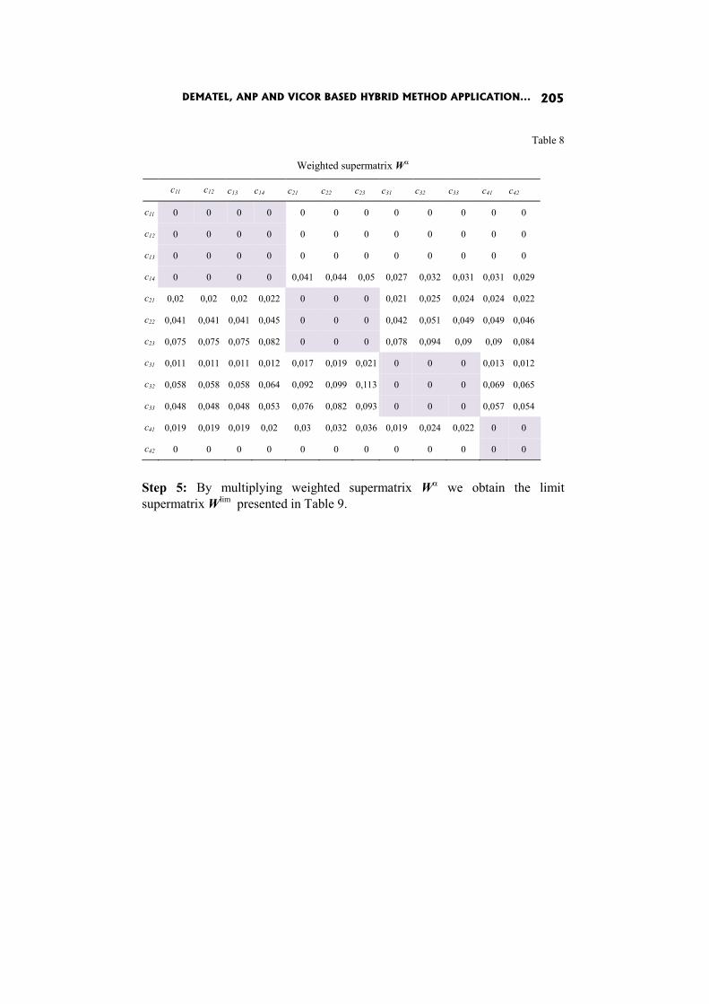
DEMATEL, ANP AND VICOR BASED HYBRID METHOD APPLICATION... 205
Table 8
Weighted supermatrix Wα
c11 c12 c13 c14 c21 c22 c23 c31 c32 c33 c41 c42
c11 0 0 0 0 0 0 0 0 0 0 0 0
c12 0 0 0 0 0 0 0 0 0 0 0 0
c13 0 0 0 0 0 0 0 0 0 0 0 0
c14 0 0 0 0 0,041 0,044 0,05 0,027 0,032 0,031 0,031 0,029
c21 0,02 0,02 0,02 0,022 0 0 0 0,021 0,025 0,024 0,024 0,022
c22 0,041 0,041 0,041 0,045 0 0 0 0,042 0,051 0,049 0,049 0,046
c23 0,075 0,075 0,075 0,082 0 0 0 0,078 0,094 0,09 0,09 0,084
c31 0,011 0,011 0,011 0,012 0,017 0,019 0,021 0 0 0 0,013 0,012
c32 0,058 0,058 0,058 0,064 0,092 0,099 0,113 0 0 0 0,069 0,065
c33 0,048 0,048 0,048 0,053 0,076 0,082 0,093 0 0 0 0,057 0,054
c41 0,019 0,019 0,019 0,02 0,03 0,032 0,036 0,019 0,024 0,022 0 0
c42 0 0 0 0 0 0 0 0 0 0 0 0 Step 5: By multiplying weighted supermatrix Wα we obtain the limit supermatrix Wlim presented in Table 9.
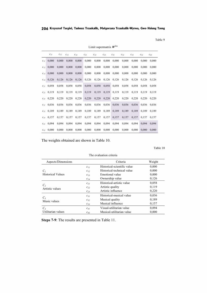
Krzysztof Targiel, Tadeusz Trzaskalik, Małgorzata Trzaskalik-Wyrwa, Gwo Hsiung Tzeng 206
Table 9
Limit supermatrix Wlim
c11 c12 c13 c14 c21 c22 c23 c31 c32 c33 c41 c42
c11 0,000 0,000 0,000 0,000 0,000 0,000 0,000 0,000 0,000 0,000 0,000 0,000
c12 0,000 0,000 0,000 0,000 0,000 0,000 0,000 0,000 0,000 0,000 0,000 0,000
c13 0,000 0,000 0,000 0,000 0,000 0,000 0,000 0,000 0,000 0,000 0,000 0,000
c14 0,126 0,126 0,126 0,126 0,126 0,126 0,126 0,126 0,126 0,126 0,126 0,126
c21 0,058 0,058 0,058 0,058 0,058 0,058 0,058 0,058 0,058 0,058 0,058 0,058
c22 0,119 0,119 0,119 0,119 0,119 0,119 0,119 0,119 0,119 0,119 0,119 0,119
c23 0,220 0,220 0,220 0,220 0,220 0,220 0,220 0,220 0,220 0,220 0,220 0,220
c31 0,036 0,036 0,036 0,036 0,036 0,036 0,036 0,036 0,036 0,036 0,036 0,036
c32 0,189 0,189 0,189 0,189 0,189 0,189 0,189 0,189 0,189 0,189 0,189 0,189
c33 0,157 0,157 0,157 0,157 0,157 0,157 0,157 0,157 0,157 0,157 0,157 0,157
c41 0,094 0,094 0,094 0,094 0,094 0,094 0,094 0,094 0,094 0,094 0,094 0,094
c42 0,000 0,000 0,000 0,000 0,000 0,000 0,000 0,000 0,000 0,000 0,000 0,000 The weights obtained are shown in Table 10.
Table 10
The evaluation criteria
Aspects/Dimensions Criteria Weight
C1 Historical Values
c11 Historical-scientific value 0,000 c12 Historical-technical value 0,000 c13 Emotional value 0,000 c14 Ownership value 0,126
C2 Artistic values
c21 Historical-artistic value 0,058 c22 Artistic quality 0,119 c23 Artistic influence 0,220
C3 Music values
c31 Historical-musical value 0,036 c32 Musical quality 0,189 c33 Musical influence 0,157
C4 Utilitarian values
c41 Visual-utilitarian value 0,094 c42 Musical-utilitarian value 0,000
Steps 7-9: The results are presented in Table 11.
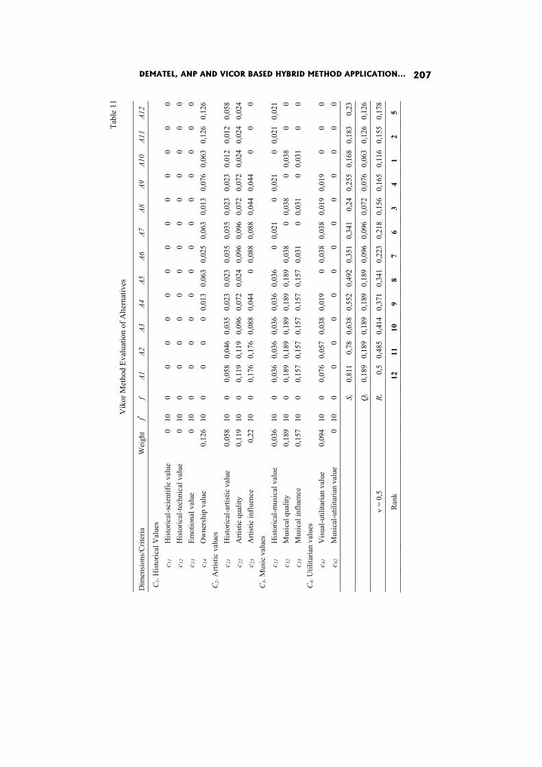
Tabl
e 11
V
ikor
Met
hod
Eval
uatio
n of
Alte
rnat
ives
Dim
ensi
ons/
Crit
eria
W
eigh
tf*
f- A1
A2
A3
A4
A5
A6
A7
A8
A9
A1
0 A1
1 A1
2
C 1. H
isto
rical
Val
ues
c 11
His
toric
al-s
cien
tific
val
ue
010
0
00
0 0
00
00
00
00
c 1
2 H
isto
rical
-tech
nica
l val
ue
010
0
00
0 0
00
00
00
00
c 13
Emot
iona
l val
ue
010
0
00
0 0
00
00
00
00
c 14
Ow
ners
hip
valu
e
0,12
610
0
00
0 0,
013
0,06
30,
025
0,06
30,
013
0,07
60,
063
0,12
60,
126
C 2. A
rtist
ic v
alue
s
c 2
1 H
isto
rical
-arti
stic
val
ue
0,05
810
0
0,05
80,
046
0,03
5 0,
023
0,02
30,
035
0,03
50,
023
0,02
30,
012
0,01
20,
058
c 22
Arti
stic
qua
lity
0,
119
10
0 0,
119
0,11
90,
096
0,07
20,
024
0,09
60,
096
0,07
20,
072
0,02
40,
024
0,02
4c 2
3 A
rtist
ic in
fluen
ce
0,22
10
0 0,
176
0,17
60,
088
0,04
40
0,08
80,
088
0,04
40,
044
00
0C 3
. Mus
ic v
alue
s
c 3
1 H
isto
rical
-mus
ical
val
ue
0,03
610
0
0,03
60,
036
0,03
6 0,
036
0,03
60
0,02
10
0,02
10
0,02
10,
021
c 32
Mus
ical
qua
lity
0,
189
10
0 0,
189
0,18
90,
189
0,18
90,
189
0,03
80
0,03
80
0,03
80
0c 3
3 M
usic
al in
fluen
ce
0,15
710
0
0,15
70,
157
0,15
7 0,
157
0,15
70,
031
00,
031
00,
031
00
C 4. U
tilita
rian
valu
es
c 4
1 V
isua
l-util
itaria
n va
lue
0,
094
10
0 0,
076
0,05
70,
038
0,01
90
0,03
80,
038
0,01
90,
019
00
0c 4
2 M
usic
al-u
tilita
rian
valu
e
010
0
00
0 0
00
00
00
00
S i
0,81
10,
780,
638
0,55
20,
492
0,35
10,
341
0,24
0,25
50,
168
0,18
30,
23
Qi
0,18
90,
189
0,18
9 0,
189
0,18
90,
096
0,09
60,
072
0,07
60,
063
0,12
60,
126
ν =
0,5
R i
0,
50,
485
0,41
4 0,
371
0,34
10,
223
0,21
80,
156
0,16
50,
116
0,15
50,
178
Ran
k
12
11
10
9
8 7
6 3
4 1
2 5
DEMATEL, ANP AND VICOR BASED HYBRID METHOD APPLICATION... 207
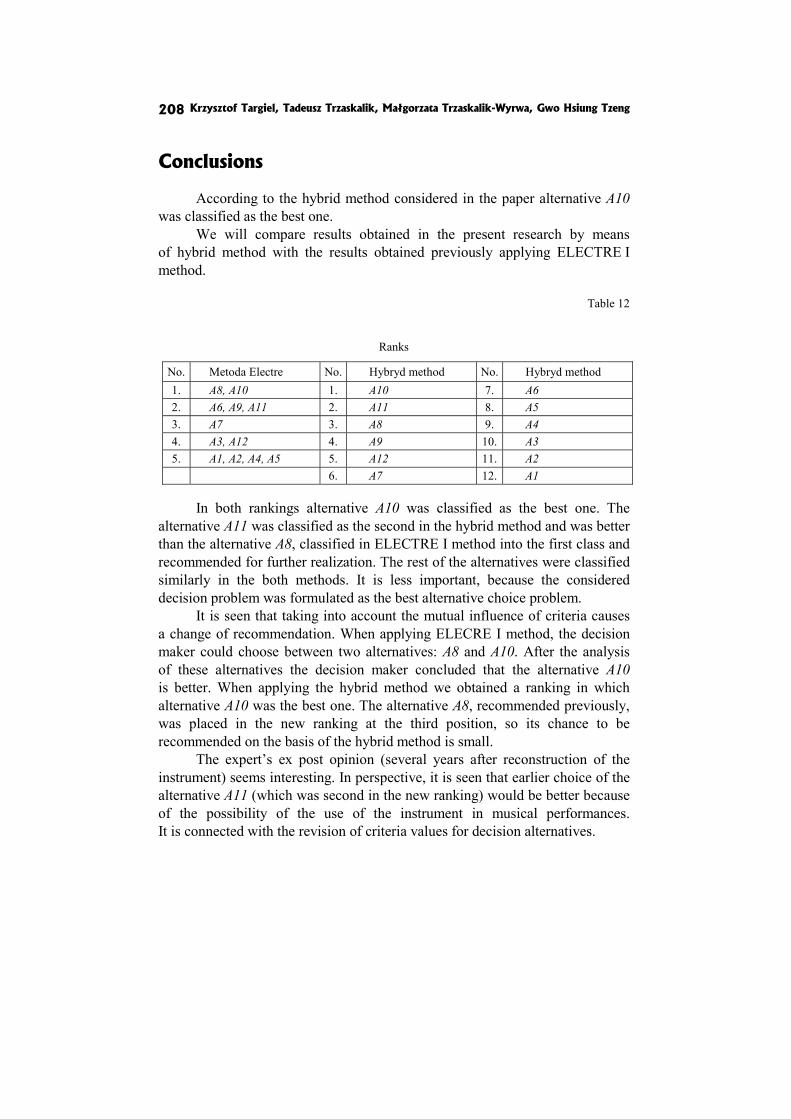
Krzysztof Targiel, Tadeusz Trzaskalik, Małgorzata Trzaskalik-Wyrwa, Gwo Hsiung Tzeng 208
Conclusions
According to the hybrid method considered in the paper alternative A10 was classified as the best one.
We will compare results obtained in the present research by means of hybrid method with the results obtained previously applying ELECTRE I method.
Table 12
Ranks
No. Metoda Electre No. Hybryd method No. Hybryd method 1. A8, A10 1. A10 7. A6 2. A6, A9, A11 2. A11 8. A5 3. A7 3. A8 9. A4 4. A3, A12 4. A9 10. A3 5. A1, A2, A4, A5 5. A12 11. A2
6. A7 12. A1
In both rankings alternative A10 was classified as the best one. The alternative A11 was classified as the second in the hybrid method and was better than the alternative A8, classified in ELECTRE I method into the first class and recommended for further realization. The rest of the alternatives were classified similarly in the both methods. It is less important, because the considered decision problem was formulated as the best alternative choice problem.
It is seen that taking into account the mutual influence of criteria causes a change of recommendation. When applying ELECRE I method, the decision maker could choose between two alternatives: A8 and A10. After the analysis of these alternatives the decision maker concluded that the alternative A10 is better. When applying the hybrid method we obtained a ranking in which alternative A10 was the best one. The alternative A8, recommended previously, was placed in the new ranking at the third position, so its chance to be recommended on the basis of the hybrid method is small.
The expert’s ex post opinion (several years after reconstruction of the instrument) seems interesting. In perspective, it is seen that earlier choice of the alternative A11 (which was second in the new ranking) would be better because of the possibility of the use of the instrument in musical performances. It is connected with the revision of criteria values for decision alternatives.
DEMATEL, ANP AND VICOR BASED HYBRID METHOD APPLICATION... 209
The alternative A11 recommends reconstruction of the whole sound system according to preserved models. This solution gives the possibility of uncomprising use of the new pipes to obtain satisfactory level of sound. The conservation of several original pipes and the adjustment to them the rest of reconstructed pipes to their loudness caused an additional adverse result (among other problems) that the instrument plays too softly, and the “historical” timbre makes up for this insufficiently.
Also, the problem of hypothetical shape of wood-carver’s decorations in upper box windows (not hitherto reconstructed) could be positively solved now, as not causing damage to historical substance and, at the same time considerably increasing visual attraction of the monument.
The knowledge obtained during the decision process and later can be used in conservation works in the future.
The recommendation of the alternative A8 (first compared with the alternative A10 while performing ELECTRE I analysis) was prepared by the expert on the merits of the case. The merits and arguments from the field of historical objects restoration should be the most important – the ranking (of course significant) is of auxiliary importance.
A detailed analysis of the hybrid method assumptions and justification of joint applications of DEMATEL, ANP and VICOR methods is a separate problem. Such an analysis has not been performed yet and it should be presented in future research.
Acknowledgements
This study is partially supported by the grant from Polish Ministry of Science and Higher Education, project number NN 111 2350 36 and granted (No. 099 WMRFD1717003) by National Science Council – Taiwan and Polish Academy of Science as of the international academic collaboration program (Taiwan – Poland) Turing the years 2011-2012.
References
Fontela E., Gabus A. (1974), DEMATEL. Innovative Methods. Raport No. 2, Structural Analysis of the World Problematique, Battelle Geneva Research Institute.
Liu C.H., Tzeng, G.H., Lee, M.H. (2012), Improving Tourism Policy Implementation – The Use of Hybrid MCDM Models, “Tourism Management”, Vol. 33.
Opricovic S., Tzeng G.H. (2007), Extended VICOR Method in Comparison with Out-ranking Methods, “European Journal of Operational Research”, No. 178(2).

Krzysztof Targiel, Tadeusz Trzaskalik, Małgorzata Trzaskalik-Wyrwa, Gwo Hsiung Tzeng 210
Saaty T.L. (1999), Fundamentals of the Analytic Network Process, International Sym-posium on the Analytic Hierarchy Process, Kobe.
Trzaskalik-Wyrwa M., Nowak M., Trzaskalik T. (2006), Application of Multicriteria Analysis to Restoration of Historical Portable Organ, [in:] Multiple Criteria Decision Making’05, ed.T. Trzaskalik, Wydawnictwo AE, Katowice.
Tzeng G.H., Chiang C.-H., Li C.-W. (2007), Evaluating Intertwined Effects in e-Lear-ning Programs: A Novel Hybrid MCDM Model Based on Factor Analysis and DEMATEL, “Expert Systems with Applications”, Vol. 32.
Tzeng G.H., Huang J.J. (2011), Multiple Attribute Decision Making: Methods and Applications, Chapman and Hall/CRC.

İrem Uçal Sari
Dorota Kuchta*
MULTICRITERIA EVALUATION OF FUZZY NET PRESENT VALUE
1
Abstract
In this paper it is shown how to assess the degree of influence of various factors on the value of the project (NPV). The assessment is based on grouping and ranking of cash flows linked to various factors. The formulas are generated both for crisp and fuzzy net present value analysis. The projects are then evaluated on the basis of at least two criteria: the NPV and the risk (positive or negative) linked to the factors which have most influence on the project’s NPV whose change may change the NPV considerably. In applications, fuzzy present values of different factors are calculated and compared for two different cases.
Keywords
Fuzzy Logic, Fuzzy Net Present Value, Ranking Fuzzy Numbers.
Introduction
Investment decisions are strategic decisions, which directly affect the position of a firm in the market. One of the most important criteria used to select an investment project is its worth for the decision makers. The discounted cash flows analyses (mostly net present value (NPV) analysis) are preferred to evaluate the investment projects. The NPV of a project, calculated before the beginning of the project, is the most widely used criterion to evaluate a project – it is generally accepted that the higher the NPV, the better the project.
However, things are not as simple that. It is widely known that investment decisions are always exposed to a high degree of uncertainty
* Corresponding author. 1 This research paper was developed under the financial support of TUBITAK (The Scientific and Techno-
logical Research Council of Turkey).
İrem Uçal Sari, Dorota Kuchta 212
and risk. Thus, the NPV cannot be the only project selection criterion, because it may change and be in reality, once the project is implemented, substantially different from its planned value. That is why each investment project has to be evaluated taking into account more than just this one criterion. It is widely agreed that the risk of the project has to be taken into account too.
If risk is understood both in the negative (as a possible threat) and positive (as a possible chance), it is good to know where risk lies in a given investment project and which factor can change or be changed in such a way that its influence on the NPV of the project would be high. Each investment project is influenced by several factors, which may be dependent or independent of the company in question (behavior and situation of the customers and suppliers, payment conditions, prices, “make or buy” decisions etc.). The aim of the paper is to show how these factors and their possible influence on the project value can be identified. Each project should then be evaluated on the basis of its NPV and of the risk of a change in the NPV, linked to various factors influencing the value of the project.
What is more, as each investment project is a long-term project and its parameters are always connected with risk and uncertainty, we consider here the fuzzy approach to the estimation of the project’s parameters. Fuzzy numbers allow us to model the incomplete knowledge about cash flows in the future.
The outline of the paper is as follows: first we present the classical approach to the evaluation of investment projects, but extending the classical definition of the NPV so that different factors influencing it, as well as their degree of influence, may be identified. Then we briefly describe the fundamentals of the fuzzy logic [Zadeh 1965; Ross 1995]. Finally the fuzzy approach to investment project evaluation is presented [Chio and Park 1994; Kuchta 2000; Zhang et al. 2011; Sorenson and Lavelle 2008], into which we incorporate the proposed approach taking into account those factors which influence the NPV. Subsequently, we present one of several possible approaches to fuzzy numbers ranking, which will be needed while estimating the “force” of individual factors influencing the NPV. The approach chosen permits to adjust the method to the attitude of the decision maker (pessimistic or optimistic). The paper concludes with two numerical examples.
1. Net Present Value Analysis
One of the most used discounted cash flow analysis method is net present value analysis which is calculated by adding up the present values of all cash flows into or out of the project.
MULTICRITERIA EVALUATION OF FUZZY NET PRESENT VALUE 213
The basic formula of present value of a single future payment ( ( )) at the end of year from now is given in Eq. 1.1 where stands for the amount of the payment and stands for the compound interest rate. ( ) = 1(1 + ) (1.1)
The formula of net present value of a cash flow series ( ( , … )) which has different payments is calculated by Eq. 1.2 where stands for the amount of the payment and stands for the time period of the payment. ( , … ) = − + ( ) + ( ) + + ⋯ + 1(1 + )
(1.2)
Sometimes the initial investment of the project can be distributed over several years. Eq. 1.3 gives NPV when the initial investment is distributed over z years: = − − 1(1 + ) − 1(1 + ) − ⋯ − 1(1 + ) +
+ 1(1 + ) + 1(1 + ) + ⋯ + 1(1 + ) (1.3)
The NPV is influenced by several factors. Sometimes small changes in some cash flow factors could be introduced − or occur independently of us − which result in a substantially better or worse NPV. For example, if the NPV is strongly influenced by labor costs, the decision maker could prefer to hire lower qualified workers or to outsource the work. If the factors influencing strongly the NPV are the payment conditions offered to the customers, the deadlines of the payments could be changed. Sometimes the NPV may be very sensitive to the situation of one of the customers or the suppliers. At that point, the decision maker may want to know the degree of influence of the situation of a given customer or supplier, of the chosen resources, suppliers, payment conditions etc. on the net present value of the project.
We propose, thus, to reorder the cash flow from Eq. (1.3) into groups of influence: each group consists of cash flows which depend on one specific factor (e.g. the situation of one customer, the decision to hire a certain workforce etc.). Of course, we assume that such reordering is possible – that it is possible to classify the cash flows into such groups which are influenced mainly by one factor. It is a limiting assumption, but less limiting than that – generally assumed − about the independence of the cash flows in subsequent
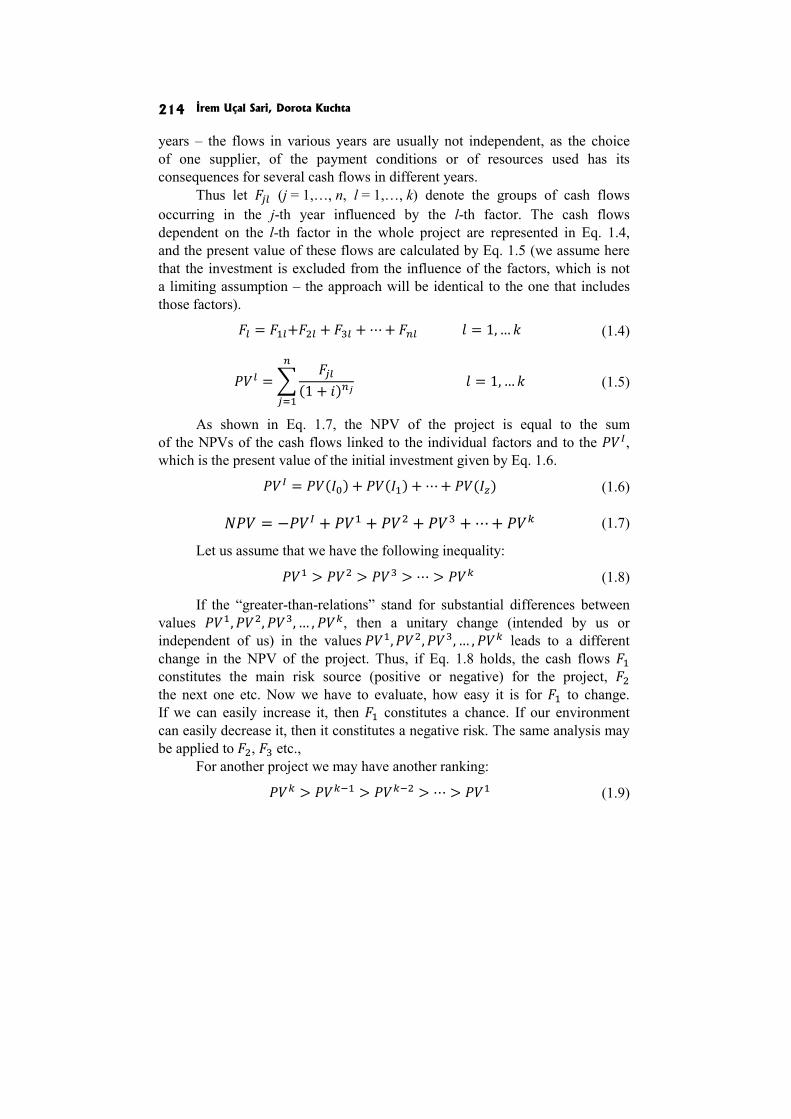
İrem Uçal Sari, Dorota Kuchta 214
years – the flows in various years are usually not independent, as the choice of one supplier, of the payment conditions or of resources used has its consequences for several cash flows in different years.
Thus let (j = 1,…, n, l = 1,…, k) denote the groups of cash flows occurring in the j-th year influenced by the l-th factor. The cash flows dependent on the l-th factor in the whole project are represented in Eq. 1.4, and the present value of these flows are calculated by Eq. 1.5 (we assume here that the investment is excluded from the influence of the factors, which is not a limiting assumption – the approach will be identical to the one that includes those factors). = + + + ⋯ + = 1, … (1.4)
= (1 + ) = 1, … (1.5)
As shown in Eq. 1.7, the NPV of the project is equal to the sum of the NPVs of the cash flows linked to the individual factors and to the , which is the present value of the initial investment given by Eq. 1.6. = ( ) + ( ) + ⋯ + ( ) (1.6)= − + + + + ⋯ + (1.7)
Let us assume that we have the following inequality: > > > ⋯ > (1.8)
If the “greater-than-relations” stand for substantial differences between values , , , … , , then a unitary change (intended by us or independent of us) in the values , , , … , leads to a different change in the NPV of the project. Thus, if Eq. 1.8 holds, the cash flows constitutes the main risk source (positive or negative) for the project, the next one etc. Now we have to evaluate, how easy it is for to change. If we can easily increase it, then constitutes a chance. If our environment can easily decrease it, then it constitutes a negative risk. The same analysis may be applied to , etc.,
For another project we may have another ranking: > > > ⋯ > (1.9)
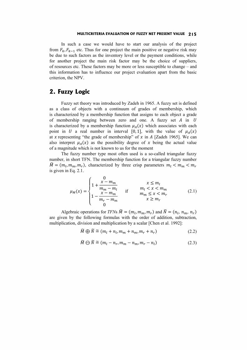
MULTICRITERIA EVALUATION OF FUZZY NET PRESENT VALUE 215
In such a case we would have to start our analysis of the project from , etc. Thus for one project the main positive or negative risk may be due to such factors as the inventory level or the payment conditions, while for another project the main risk factor may be the choice of suppliers, of resources etc. These factors may be more or less susceptible to change – and this information has to influence our project evaluation apart from the basic criterion, the NPV.
2. Fuzzy Logic
Fuzzy set theory was introduced by Zadeh in 1965. A fuzzy set is defined as a class of objects with a continuum of grades of membership, which is characterized by a membership function that assigns to each object a grade of membership ranging between zero and one. A fuzzy set in is characterized by a membership function ( ) which associates with each point in a real number in interval [0, 1], with the value of ( ) at representing “the grade of membership” of in [Zadeh 1965]. We can also interpret ( ) as the possibility degree of being the actual value of a magnitude which is not known to us for the moment
The fuzzy number type most often used is a so-called triangular fuzzy number, in short TFN. The membership function for a triangular fuzzy number = ( , , ), characterized by three crisp parameters < < is given in Eq. 2.1.
( ) =01 + −−1 − −−0
if ≤< <≤ <≥ (2.1)
Algebraic operations for TFNs = ( , , ) and = ( , , ) are given by the following formulas with the order of addition, subtraction, multiplication, division and multiplication by a scalar [Chen et al. 1992]: ⊕ = ( + , + , + ) (2.2)⊖ = ( − , − , − ) (2.3)

İrem Uçal Sari, Dorota Kuchta 216
⨂ = ( , , ) ≥ 0, ≥ 0( , , ) if ≤ 0, ≥ 0( , , ) ≤ 0, ≤ 0 (2.4)
⊘ = , , ≥ 0, ≥ 0, , if ≤ 0, ≥ 0, , ≤ 0, ≤ 0 (2.5)
λ⨂ = ( , , )( , , ) if ≥ 0≤ 0 ∀ ∈ ℛ (2.6)
The support of a fuzzy number = ( , , ) is the interval [ , ] − thus the domain on which the membership function takes on positive values, together with its boundary. The support of will be denoted as .
3. Fuzzy Net Present Value
Fuzzy present value of a single future payment ( ( )) occurred at the end of year from now is given in Eq. 3.1 where stands for fuzzy amount of the payment and stands for the compound interest rate. ( ) = (1 + ) (3.1)
Kuchta [2000] defined the general formula of fuzzy net present value as given in Eq. 3.2, where denotes net cash flows in the time period and ı̃ denotes the fuzzy interest rate. = − + (1 + )̃ (3.2)
The formula of fuzzy net present value of a project ( ) which has different payments and has an initial investment at the beginning of the project is calculated by Eq. 3.3.
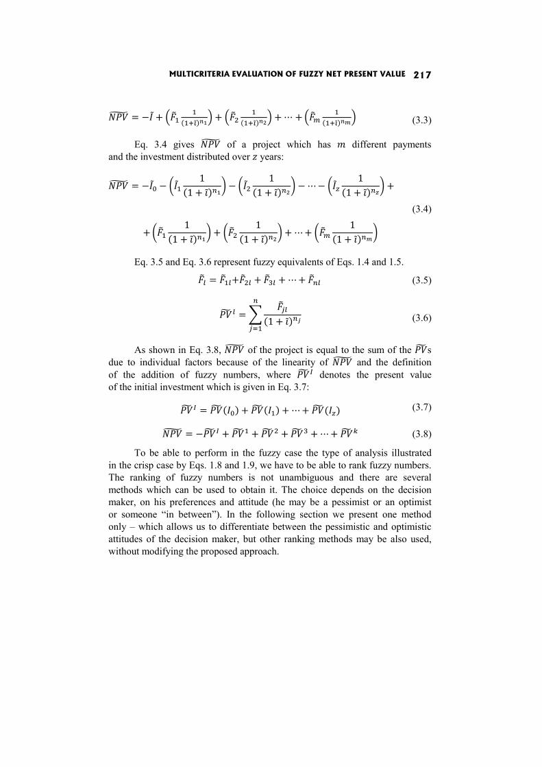
MULTICRITERIA EVALUATION OF FUZZY NET PRESENT VALUE 217
= − + ( ̃) + ( ̃) + ⋯ + ( ̃) (3.3)
Eq. 3.4 gives of a project which has different payments and the investment distributed over years:
= − − 1(1 + ̃) − 1(1 + )̃ − ⋯ − 1(1 + ̃) + + 1(1 + )̃ + 1(1 + )̃ + ⋯ + 1(1 + ̃)
(3.4)
Eq. 3.5 and Eq. 3.6 represent fuzzy equivalents of Eqs. 1.4 and 1.5. = + + + ⋯ + (3.5)
= (1 + ̃) (3.6)
As shown in Eq. 3.8, of the project is equal to the sum of the s due to individual factors because of the linearity of and the definition of the addition of fuzzy numbers, where denotes the present value of the initial investment which is given in Eq. 3.7: = ( ) + ( ) + ⋯ + ( ) (3.7)= − + + + + ⋯ + (3.8)
To be able to perform in the fuzzy case the type of analysis illustrated in the crisp case by Eqs. 1.8 and 1.9, we have to be able to rank fuzzy numbers. The ranking of fuzzy numbers is not unambiguous and there are several methods which can be used to obtain it. The choice depends on the decision maker, on his preferences and attitude (he may be a pessimist or an optimist or someone “in between”). In the following section we present one method only – which allows us to differentiate between the pessimistic and optimistic attitudes of the decision maker, but other ranking methods may be also used, without modifying the proposed approach.
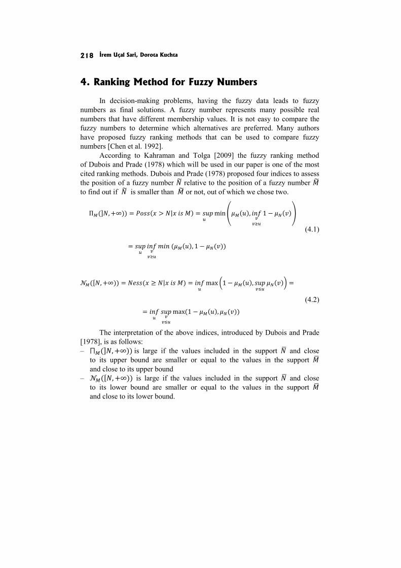
İrem Uçal Sari, Dorota Kuchta 218
4. Ranking Method for Fuzzy Numbers
In decision-making problems, having the fuzzy data leads to fuzzy numbers as final solutions. A fuzzy number represents many possible real numbers that have different membership values. It is not easy to compare the fuzzy numbers to determine which alternatives are preferred. Many authors have proposed fuzzy ranking methods that can be used to compare fuzzy numbers [Chen et al. 1992].
According to Kahraman and Tolga [2009] the fuzzy ranking method of Dubois and Prade (1978) which will be used in our paper is one of the most cited ranking methods. Dubois and Prade (1978) proposed four indices to assess the position of a fuzzy number relative to the position of a fuzzy number to find out if is smaller than or not, out of which we chose two.
Π (] , +∞)) = ( > | ) = min ( ), 1 − ( )
= ( ( ), 1 − ( ))
(4.1)
([ , +∞)) = ( ≥ | ) = max 1 − ( ), ( ) =
= max(1 − ( ), ( ))
(4.2)
The interpretation of the above indices, introduced by Dubois and Prade [1978], is as follows: – ⨅ (] , +∞)) is large if the values included in the support and close
to its upper bound are smaller or equal to the values in the support and close to its upper bound
– ([ , +∞)) is large if the values included in the support and close to its lower bound are smaller or equal to the values in the support and close to its lower bound.
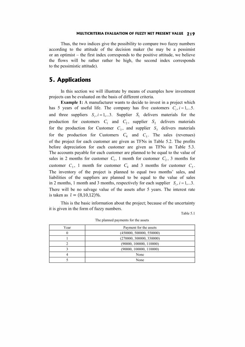
MULTICRITERIA EVALUATION OF FUZZY NET PRESENT VALUE 219
Thus, the two indices give the possibility to compare two fuzzy numbers according to the attitude of the decision maker (he may be a pessimist or an optimist – the first index corresponds to the positive attitude, we believe the flows will be rather rather be high, the second index corresponds to the pessimistic attitude).
5. Applications
In this section we will illustrate by means of examples how investment projects can be evaluated on the basis of different criteria.
Example 1: A manufacturer wants to decide to invest in a project which has 5 years of useful life. The company has five customers .5,...1, =iCi and three suppliers .3,...1, =iSi Supplier 1S delivers materials for the production for customers 1C and 2C , supplier 2S delivers materials for the production for Customer 3C , and supplier 3S delivers materials for the production for Customers 4C and 5C . The sales (revenues) of the project for each customer are given as TFNs in Table 5.2. The profits before depreciation for each customer are given as TFNs in Table 5.3. The accounts payable for each customer are planned to be equal to the value of sales in 2 months for customer 1C , 1 month for customer 2C , 3 months for customer 3C , 1 month for customer 4C and 3 months for customer 5C . The inventory of the project is planned to equal two months’ sales, and liabilities of the suppliers are planned to be equal to the value of sales in 2 months, 1 month and 3 months, respectively for each supplier .3,...1, =iSi There will be no salvage value of the assets after 5 years. The interest rate is taken as ̃ = (8,10,12)%.
This is the basic information about the project; because of the uncertainty it is given in the form of fuzzy numbers.
Table 5.1
The planned payments for the assets
Year Payment for the assets 0 (450000, 500000, 550000) 1 (270000, 300000, 330000) 2 (90000, 100000, 110000) 3 (90000, 100000, 110000) 4 None 5 None
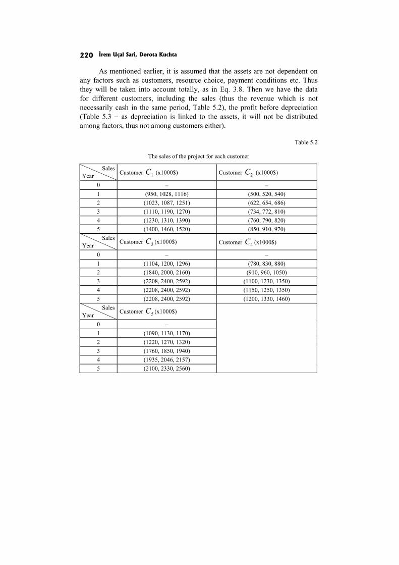
İrem Uçal Sari, Dorota Kuchta 220
As mentioned earlier, it is assumed that the assets are not dependent on any factors such as customers, resource choice, payment conditions etc. Thus they will be taken into account totally, as in Eq. 3.8. Then we have the data for different customers, including the sales (thus the revenue which is not necessarily cash in the same period, Table 5.2), the profit before depreciation (Table 5.3 − as depreciation is linked to the assets, it will not be distributed among factors, thus not among customers either).
Table 5.2
The sales of the project for each customer
Sales Year Customer 1C (x1000$) Customer 2C (x1000$)
0 − − 1 (950, 1028, 1116) (500, 520, 540) 2 (1023, 1087, 1251) (622, 654, 686) 3 (1110, 1190, 1270) (734, 772, 810) 4 (1230, 1310, 1390) (760, 790, 820) 5 (1400, 1460, 1520) (850, 910, 970)
Sales Year Customer 3C (x1000$) Customer 4C (x1000$)
0 − − 1 (1104, 1200, 1296) (780, 830, 880) 2 (1840, 2000, 2160) (910, 960, 1050) 3 (2208, 2400, 2592) (1100, 1230, 1350) 4 (2208, 2400, 2592) (1150, 1250, 1350) 5 (2208, 2400, 2592) (1200, 1330, 1460)
Sales Year Customer 5C (x1000$)
0 − 1 (1090, 1130, 1170) 2 (1220, 1270, 1320) 3 (1760, 1850, 1940) 4 (1935, 2046, 2157) 5 (2100, 2330, 2560)
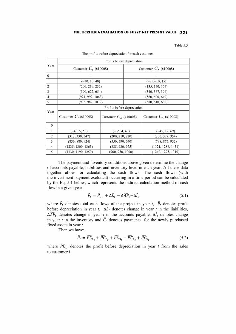
MULTICRITERIA EVALUATION OF FUZZY NET PRESENT VALUE 221
Table 5.3
The profits before depreciation for each customer
Year
Profits before depreciation
Customer 1C (x1000$) Customer 2C (x1000$)
0 − − 1 (−30, 10, 40) (−35,−10, 15) 2 (206, 219, 232) (135, 150, 165) 3 (590, 622, 654) (340, 367, 394) 4 (921, 992, 1063) (560, 600, 640) 5 (935, 987, 1039) (580, 610, 630) Year
Profits before depreciation
Customer 3C (x1000$) Customer 4C (x1000$) Customer 5C (x1000$)
0 − − − 1 (−48, 5, 58) (−35, 4, 43) (−45, 12, 69) 2 (313, 330, 347) (200, 210, 220) (300, 327, 354) 3 (836, 880, 924) (550, 590, 640) (798, 875, 952) 4 (1235, 1300, 1365) (885, 930, 975) (1121, 1286, 1451) 5 (1130, 1190, 1250) (900, 950, 1000) (1240, 1275, 1310)
The payment and inventory conditions above given determine the change
of accounts payable, liabilities and inventory level in each year. All these data together allow for calculating the cash flows. The cash flows (with the investment payment excluded) occurring in a time period can be calculated by the Eq. 5.1 below, which represents the indirect calculation method of cash flow in a given year: = + ∆ − ∆ −∆ (5.1)
where denotes total cash flows of the project in year t, denotes profit before depreciation in year t, ∆ denotes change in year t in the liabilities, ∆ denotes change in year t in the accounts payable, ∆ denotes change in year t in the inventory and denotes payments for the newly purchased fixed assets in year t.
Then we have: = + + + + (5.2)
where denotes the profit before depreciation in year t from the sales to customer .
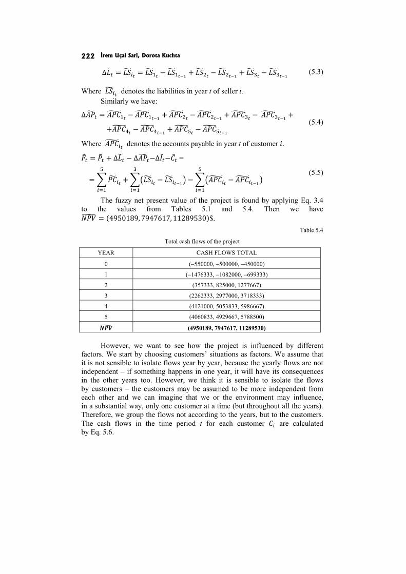
İrem Uçal Sari, Dorota Kuchta 222 ∆ = = − + − + − (5.3)
Where denotes the liabilities in year t of seller . Similarly we have: ∆ = − + − + − + + − + −
(5.4)
Where denotes the accounts payable in year t of customer . = + ∆ − ∆ −∆ − =
= + − − − (5.5)
The fuzzy net present value of the project is found by applying Eq. 3.4 to the values from Tables 5.1 and 5.4. Then we have = (4950189, 7947617, 11289530)$.
Table 5.4
Total cash flows of the project
YEAR CASH FLOWS TOTAL
0 (−550000, −500000, −450000)
1 (−1476333, −1082000, −699333)
2 (357333, 825000, 1277667)
3 (2262333, 2977000, 3718333)
4 (4121000, 5053833, 5986667)
5 (4060833, 4929667, 5788500)
(4950189, 7947617, 11289530) However, we want to see how the project is influenced by different
factors. We start by choosing customers’ situations as factors. We assume that it is not sensible to isolate flows year by year, because the yearly flows are not independent – if something happens in one year, it will have its consequences in the other years too. However, we think it is sensible to isolate the flows by customers – the customers may be assumed to be more independent from each other and we can imagine that we or the environment may influence, in a substantial way, only one customer at a time (but throughout all the years). Therefore, we group the flows not according to the years, but to the customers. The cash flows in the time period t for each customer are calculated by Eq. 5.6.

MULTICRITERIA EVALUATION OF FUZZY NET PRESENT VALUE 223= + Δ − Δ (5.6)
where denotes cash flows of the project for customer in year t, denotes profit before depreciation for customer in year t, Δ denotes change in year t in the liabilities of the supplier (suppliers) of the product for customer , Δ denotes change in year t in the accounts payable for customer .
The present value of the total cash flows linked to each customer is found from Eq. 5.7. ( ) = ∑(1 + ) = ∑ + Δ − Δ(1 + ) (5.7)
Here are the values ( ), = 1, … ,5
Table 5.5
The values ( ), = 1, … ,5
Year
Present value of cash flows
Customer 1C (x1000$)
Customer 2C (x1000$)
0 − − 1 (−217560, −146667, −83951) (−77381, −48485, −18519) 2 (71880, 172865, 268490) (81447, 114738, 150463) 3 (344620, 454420, 589156) (214246, 268345, 328117) 4 (521760, 663889, 825439) (336931, 408784, 490142) 5 (476639, 597326, 737752) (302155, 372553, 447483)
Year
Present value of cash flows
Customer 3C
(x1000$) Customer 4C
(x1000$)
Customer 5C
(x1000$) 0 − − −
1 (−442857, −359091, −272222) (−53571, 3636, 62963) (−232143, −160303, −85802
2 (−65104, 52342, 178612) (111607, 173554, 240055) (172725, 250964, 334934) 3 (374871, 560982, 767371) (322081, 443276, 585451) (432762, 584773, 753082) 4 (662845, 887917, 1144441) (490938, 635203, 799345) (606496, 856044, 1141011) 5 (532246, 738896, 981401) (445430, 589875, 758850) (547756, 762284, 1014069)
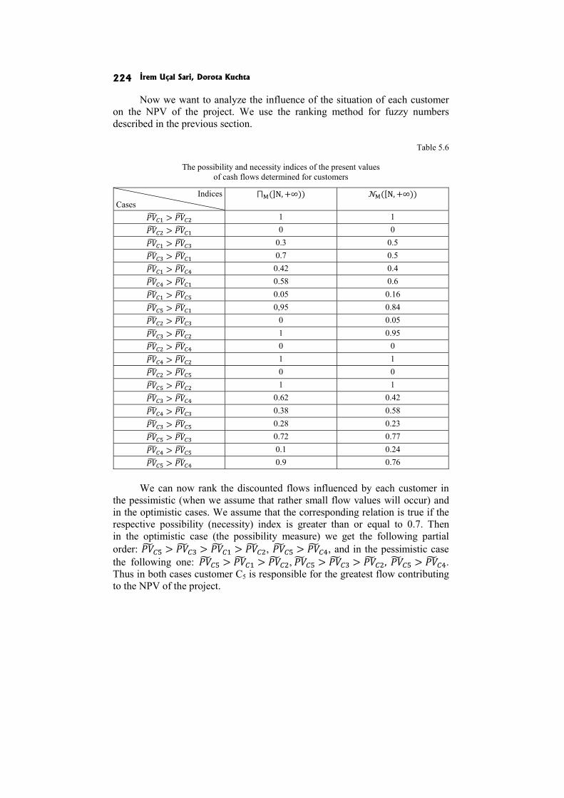
İrem Uçal Sari, Dorota Kuchta 224
Now we want to analyze the influence of the situation of each customer on the NPV of the project. We use the ranking method for fuzzy numbers described in the previous section.
Table 5.6
The possibility and necessity indices of the present values
of cash flows determined for customers
Indices Cases
⨅ (]N, +∞)) ([N, +∞)) > 1 1 > 0 0 > 0.3 0.5 > 0.7 0.5 > 0.42 0.4 > 0.58 0.6 > 0.05 0.16 > 0,95 0.84 > 0 0.05 > 1 0.95 > 0 0 > 1 1 > 0 0 > 1 1 > 0.62 0.42 > 0.38 0.58 > 0.28 0.23 > 0.72 0.77 > 0.1 0.24 > 0.9 0.76
We can now rank the discounted flows influenced by each customer in
the pessimistic (when we assume that rather small flow values will occur) and in the optimistic cases. We assume that the corresponding relation is true if the respective possibility (necessity) index is greater than or equal to 0.7. Then in the optimistic case (the possibility measure) we get the following partial order: > > > , > , and in the pessimistic case the following one: > > , > > , > . Thus in both cases customer C5 is responsible for the greatest flow contributing to the NPV of the project.
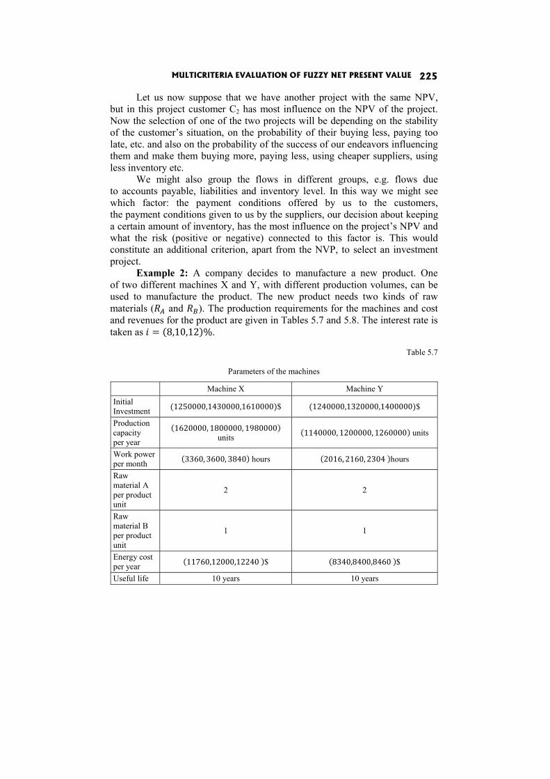
MULTICRITERIA EVALUATION OF FUZZY NET PRESENT VALUE 225
Let us now suppose that we have another project with the same NPV, but in this project customer C2 has most influence on the NPV of the project. Now the selection of one of the two projects will be depending on the stability of the customer’s situation, on the probability of their buying less, paying too late, etc. and also on the probability of the success of our endeavors influencing them and make them buying more, paying less, using cheaper suppliers, using less inventory etc.
We might also group the flows in different groups, e.g. flows due to accounts payable, liabilities and inventory level. In this way we might see which factor: the payment conditions offered by us to the customers, the payment conditions given to us by the suppliers, our decision about keeping a certain amount of inventory, has the most influence on the project’s NPV and what the risk (positive or negative) connected to this factor is. This would constitute an additional criterion, apart from the NVP, to select an investment project.
Example 2: A company decides to manufacture a new product. One of two different machines X and Y, with different production volumes, can be used to manufacture the product. The new product needs two kinds of raw materials ( and ). The production requirements for the machines and cost and revenues for the product are given in Tables 5.7 and 5.8. The interest rate is taken as = (8,10,12)%.
Table 5.7
Parameters of the machines
Machine X Machine Y Initial Investment (1250000,1430000,1610000)$ (1240000,1320000,1400000)$
Production capacity per year
(1620000, 1800000, 1980000) units (1140000, 1200000, 1260000) units
Work power per month (3360, 3600, 3840) hours (2016, 2160, 2304 )hours
Raw material A per product unit
2 2
Raw material B per product unit
1 1
Energy cost per year (11760,12000,12240 )$ (8340,8400,8460 )$
Useful life 10 years 10 years

İrem Uçal Sari, Dorota Kuchta 226
Table 5.8
Costs and revenues generated by the new product
Cost or Revenue Labor cost per hour (4.5, 5, 5.5 )$ Cost of Raw material A per product (0,8,0,9,1 )$ Cost of Raw Material B per product (0.9, 1, 1.1)$ Price of the product per unit (9, 10, 11)$
Net annual cash flows and fuzzy present values of the cash flows for each
factor are calculated and given in Table 5.9.
Table 5.9
Cash Flows and Present Values of the Factors
TOTAL CASH FLOWS
Machine X Machine Y 1 2 3
Net annual cash flows (total) (8408640, 12930000, 17703120) (6332868, 8620800, 10992588)
of total cash flows (18660829, 49014873, 114812908) (14054183, 32679615, 71292009)
of the project (17050829, 47584873, 113562908) (12654183, 31359615, 70052009)
Annual Energy Cost (12240, 12000, 11760) (8460, 8400, 8340)
of Energy Costs ( )
(76269, 45489, 27164) (54089, 31843, 18775)
Annual Labor Cost (21120, 18000, 15120) (12672, 10800, 9072)
of Labor Costs ( )
(98060, 68234, 46870) (58836, 40940, 28122)
Annual raw material cost (6138000, 5040000, 4050000) (3906000, 3360000, 2850000)
of total raw material costs ( )
(26266120, 19105565, 13621724) (18483566, 12737044, 8668370)
Annual cost of raw material A (3960000, 3240000, 2592000) (2520000, 2160000, 1824000)
of raw material A costs ( )
(16810317, 12282149, 8788209) (11829482, 8188099, 5592496)
Annual cost of raw material B (2178000, 1800000, 1458000) (1386000, 1200000, 1026000)
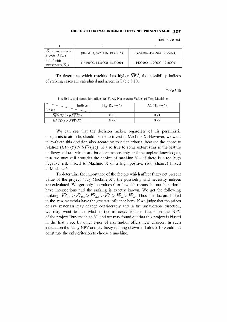
MULTICRITERIA EVALUATION OF FUZZY NET PRESENT VALUE 227
Table 5.9 contd.
1 2 3 of raw material
B costs ( ) (9455803, 6823416, 4833515) (6654084, 4548944, 3075873)
of initial investment ( )
(1610000, 1430000, 1250000) (1400000, 1320000, 1240000)
To determine which machine has higher , the possibility indices
of ranking cases are calculated and given in Table 5.10.
Table 5.10
Possibility and necessity indices for Fuzzy Net present Values of Two Machines Indices Cases ⨅ (]N, +∞)) ([N, +∞)) ( ) > ( ) 0.78 0.71( ) > ( ) 0.22 0.29
We can see that the decision maker, regardless of his pessimistic or optimistic attitude, should decide to invest in Machine X. However, we want to evaluate this decision also according to other criteria, because the opposite relation ( ( ) > ( )) is also true to some extent (this is the feature of fuzzy values, which are based on uncertainty and incomplete knowledge), thus we may still consider the choice of machine Y − if there is a too high negative risk linked to Machine X or a high positive risk (chance) linked to Machine Y.
To determine the importance of the factors which affect fuzzy net present value of the project “buy Machine X”, the possibility and necessity indices are calculated. We get only the values 0 or 1 which means the numbers don’t have intersections and the ranking is exactly known. We get the following ranking: > > > > > . Thus the factors linked to the raw materials have the greatest influence here. If we judge that the prices of raw materials may change considerably and in the unfavorable direction, we may want to see what is the influence of this factor on the NPV of the project “buy machine Y” and we may found out that this project is biased in the first place by other types of risk and/or offers new chances. In such a situation the fuzzy NPV and the fuzzy ranking shown in Table 5.10 would not constitute the only criterion to choose a machine.
İrem Uçal Sari, Dorota Kuchta 228
Conclusions
The fuzzy net present value (NPV) method is one of the most preferred investment analysis methods which can deal with the uncertainty of forecasting cash flows of investment projects. In the fuzzy net present value method the worth of an investment is defined by a fuzzy number and the decision maker has to decide whether to invest in the project by considering this number. In reality all the factors influencing fuzzy net present value of an investment should also be taken into account (e.g. the credibility of customers or suppliers, the cash flows resulting from work power, raw material selection, payment conditions etc.), together with their variability/stability. The decision maker should analyze, apart from the NPV, what is the factor which influences it most and how probable (possible) are changes in the flows linked to this factor. The final decision in the evaluation of a project should be made on the basis of NPV and the structure of its components dependent on individual factors. In the present paper we propose a method to perform such an evaluation. Further research is needed to propose a methodology of identifying different factors and verify the independence between selected groups of cash flows.
References
Chen S.J., Hwang C.L., Hwang F.P. (1992), Fuzzy Multiple Attribute Decision Making: Methods and Applications, Springer-Verlag, Berlin.
Chio C.Y, Park C.S., (1994), Fuzzy Cash Flow Analysis Using Present Worth Criterion, “The Engineering Economist”, No. 39 (2).
Dubois D., Prade H. (1978), Operations on Fuzzy Numbers, “International Journal of Systems Science”, No. 9.
Kahraman C., Tolga A.C. (2009), An Alternative Ranking Approach and its usage in Multi-criteria Decision-making, “International Journal of Computational Intelligence Systems”, No. 2(3).
Kuchta D. (2000), Fuzzy Capital Budgeting, “Fuzzy Sets and Systems”, No. 111. Ross T.J. (1995), Fuzzy Logic With Engineering Applications, Mc-Graw Hill, USA. Sorenson G.E., Lavelle J.P. (2008), A Comparison of Fuzzy Set and Probabilistic
Paradigms for Ranking Vague Economic Investment Information Using a Pre-sent Worth Criterion, “The Engineering Economist”, No. 53 (1).
Zadeh L.A. (1965): Fuzzy Sets, “Information and Control”, No. 8. Zhang W.-G., Qin M., Lu Q., Xiao W.-I., (2011), Evaluating Methods of Investment
Project and Optimizing Models of Portfolio Selection in Fuzzy Uncertainty, “Computers & Industrial Engineering”, No. 61, 3.
CONTRIBUTING AUTHORS
Marcin Anholcer Department of Operations Research Poznań University of Economics, Poland [email protected] Helena Brozova Faculty of Economics and Management Czech University of Life Science, Prague, Czech Republic [email protected] Jakub Brzostowski Institute of Mathematics Silesian University of Technology, Gliwice, Poland [email protected] Rafael Caballero Department of Applied Economics (Mathematics) University of Malaga, Spain [email protected] Cezary Dominiak Department of Operations Research University of Economics in Katowice, Poland [email protected] Petr Fiala Department of Applied Econometrics University of Economics, Prague, Czech Republic [email protected] Francisca Garcia Lopera Department of Applied Economics (Mathematics) University of Malaga, Spain [email protected] Dorota Górecka Department of Econometrics and Statistics Nicolas Copernicus University in Torun, Poland [email protected]
CONTRIBUTING AUTHORS 230
Jana Hanclova Department of Mathematical Methods in Economy VSB TU Ostrava, Czech Republic [email protected] Josef Jablonsky Department of Econometrics, University of Economics Prague, Czech Republic [email protected] Ignacy Kaliszewski Systems Research Institute Polish Academy of Science, Warsaw, Poland [email protected] Lech Kruś Systems Research Institute Polish Academy of Science, Warsaw, Poland [email protected] Bogumiła Krzeszowska Department of Operations Research University of Economics in Katowice, Poland [email protected] Dorota Kuchta Institute of Organisation and Management University of Technology, Wrocław, Poland [email protected] Jerzy Michnik Department of Operations Research University of Economics in Katowice, Poland [email protected] Janusz Miroforidis Systems Research Institute Polish Academy of Science, Warsaw, Poland [email protected] Jose Enrique Padilla Garcia Department of Applied Economics (Mathematics) University of Malaga, Spain [email protected]
CONTRIBUTING AUTHORS 231
Fatima Perez Department of Applied Economics (Mathematics) University of Malaga, Spain [email protected] Jaroslav Ramik Department of Mathematical Methods in Economics School of Business Administration in Karviná SU Opava, Czech Republic [email protected] Jan Skorupiński Institute of Control and Computation Engineering Warsaw University of Technology, Poland [email protected] Tomas Subrt Faculty of Economics and Management Czech University of Life Science, Prague, Czech Republic [email protected] Krzysztof Targiel Department of Operations Research University of Economics in Katowice, Poland [email protected] Eugeniusz Toczyłowski Institute of Control and Computation Engineering Warsaw University of Technology, Poland [email protected] Tadeusz Trzaskalik Department of Operations Research University of Economics in Katowice, Poland [email protected] Małgorzata Trzaskalik-Wyrwa Chair of Organ and Harpsichord The Fryderyk Chopin University of Music, Warsaw, Poland Diocese Siedlce, Poland [email protected]

CONTRIBUTING AUTHORS 232
Gwo Hsiung Tzeng Kainan University [email protected] Irem Uçal Sari Department of Industrial Engineering Istanbul Technical University, Macka, Istambul, Turkey [email protected] Tomasz Wachowicz Department of Operations Research University of Economics in Katowice, Poland [email protected]