MURDOCH RESEARCH REPOSITORY

This is the author’s final version of the work, as accepted for publication following peer review but without the publisher’s layout or pagination.

The definitive version is available at http://dx.doi.org/10.1016/j.biocon.2016.07.024

Tyne, J.A., Loneragan, N.R., Johnston, D.W., Pollock, K.H., Williams, R. and Bejder, L. (2016) Evaluating monitoring

methods for cetaceans. Biological Conservation, 201 . pp. 252-260.

http://researchrepository.murdoch.edu.au/34610/

Copyright © 2016 Elsevier Ltd.

1

Evaluating monitoring methods for cetaceans

Julian A. Tyne1*, Neil R. Loneragan1, David W. Johnston3,1, Kenneth H. Pollock1,2, Rob

Williams4,5 and Lars Bejder1,3

1 Murdoch University Cetacean Research Unit, School of Veterinary and Life Sciences,

Murdoch University, South Street, Murdoch, Western Australia, Australia

2 Department of Biology, North Carolina State University, Raleigh, North Carolina, United

States of America

3 Division of Marine Science and Conservation, Nicholas School of the Environment, Duke

University Marine Lab. 135 Duke Marine Lab Rd. Beaufort, North Carolina, United

States of America

4 Oceans Initiative and Oceans Research and Conservation Association, Pearse Island, British

Columbia, Canada

5 Sea Mammal Research Unit, Scottish Oceans Institute, University of St Andrews, St

Andrews, Fife, KY16 8LB, UK

* Corresponding author: j.tyne@murdoch.edu.au

Keywords:

Power analysis; Sampling effort; Hawaii spinner dolphins; Stenella longirostris; Human

pressures; Individual identification

2

Abstract

With increasing human pressures on wildlife comes a responsibility to monitor them

effectively, particularly in an environment of declining research funds. Scarce funding

resources compromise the level and efficacy of monitoring possible to detect trends in

abundance, highlighting the priority for developing cost-effective programs. A systematic

and rigorous sampling regime was developed to estimate abundance of a small, genetically

isolated spinner dolphin (Stenella longirostris) population exposed to high levels of human

activities. Five monitoring scenarios to detect trends in abundance were evaluated by

varying sampling effort, precision, power and sampling interval. Scenario 1 consisted of

monthly surveys, each of 12 days, used to obtain the initial two consecutive annual

abundance estimates. Scenarios 2, 3 and 4 consisted of a reduced effort, while Scenario 5

doubled the effort of Scenario 1. Scenarios with the greatest effort (1 and 5) produced the

most precise abundance estimates (CV=0.09). Using a CV=0.09 and power of 80%, it would

take nine years to detect a 5% annual change in abundance compared with 12 years at a

power of 95%. Under this best-case monitoring scenario, if the trend was a decline, the

population would have decreased by 37% and 46%, respectively, prior to detection of a

significant decline. With the potential of a large decline in a small population prior to

detection, the lower power level should be used to trigger a management intervention. The

approach presented here is applicable across taxa for which individuals can be identified,

including terrestrial and aquatic mammals, birds and reptiles.

3

1 Introduction

With the ever-increasing human pressure on wildlife we have a responsibility to monitor and

manage wildlife populations effectively (Geffroy et al. 2015; Tablado and Jenni 2015).

Management decisions for the conservation of wildlife should be based on sound scientific

investigations and rigorous monitoring regimes, particularly for those populations whose

viability is threatened (Jaramillo-Legorreta et al. 2007; Turvey et al. 2007). These

requirements, however, conflict with the perennial problem of scarce funding resources in

conservation biology (Williams and Thomas 2009; Williams et al. 2011). The challenge that

management agencies face is the effective allocation of scarce funding resources to

conservation research and management, while still being able to fulfil their statutory

obligations. Consequently, managers often cut the costs of research to estimate wildlife

abundance (Williams and Thomas 2009; Williams et al. 2011). The trade-off for reduced

funding for abundance estimation is a reduction in the precision of those estimates (Thomas

et al. 2010), which has important implications for the power of detecting trends in

abundance. Power analysis determines the ability of a study to detect an effect of a given

size with a degree of confidence, and should be an integral part of any study that is

investigating the demographic parameters of wildlife populations. Detecting changes in

populations is critical for managing populations with low abundance.

Taylor et al. (2007) reviewed decades of monitoring data for marine mammal stocks under

United States (U.S.) jurisdiction, and found that agencies had almost no statistical power to

detect even catastrophic declines in many stocks, especially oceanic dolphins. For example, a

study of the Atlantic spotted dolphin (Stenella frontalis) in the Western North Atlantic had

only 11% power to detect a 50% decline in 15 years (Taylor et al. 2007). In the waters of the

4

U.S., marine mammals are data-rich by global standards, as exemplified by the fact that 75%

of the world's ocean has never been surveyed to estimate cetacean density (Kaschner et al.

2012). In the face of such uncertainty, two broad approaches have been suggested as

precautionary ways to conserve marine mammal populations when statistical power is low

or data are scarce. One approach is to lower the burden of proof that a population is in

decline before triggering a mitigation approach (e.g., Taylor et al. 2000). The other is to set

allowable harm limits on an annual basis, so that populations should never decline below

some predefined threshold, as long as those annual limits are not exceeded (e.g., Wade

1998). Although these harm limits are usually thought of in terms of lethal removals from a

population (e.g., through incidental catch in fisheries or ship strikes), decision rules could be

articulated equally well in terms of the number of sub-lethal takes that policy-makers are

willing to allow animals to withstand (e.g., Higham et al. 2016).

Notwithstanding the difficulty in detecting declines in long-lived, slowly-reproducing

mammals, managers often require proof that a population falls within either the

classification of “small population” or “declining population” (Caughley 1994) before they

act. Population monitoring programs designed to detect change and determine

management strategies that hinge on proof of declines to trigger management intervention

require precise and unbiased estimates of population parameters (Taylor and Gerrodette

1993; Taylor et al. 2007). To do this, these programs must be designed to satisfy the

assumptions of the estimation methods to ensure that the estimates are unbiased and have

sufficient sampling effort to produce precise abundance estimates (Wilson et al. 1999;

Thompson et al. 2000).

5

The power to detect trends in abundance depends on the relationship between the rate of

change in the abundance, the precision of the abundance estimate (e.g., the coefficient of

variation) and the acceptable levels of making errors to detect change (Type I (α) and Type II

(β) errors). Variations in these parameters can then determine the efficacy of proposed

monitoring programs to detect trends in abundance and provide a scientific basis for the

level of precaution required to address management issues.

The U.S. National Oceanic and Atmospheric Administration (NOAA) has the mandate under

the Marine Mammal Protection Act 1972 (MMPA) to protect all cetaceans, seals and sea

lions in U.S. waters and the National Marine Fisheries Service (NMFS) and the U.S. Fish and

Wildlife Service have the responsibility for assessing the stocks of cetaceans and pinnipeds.

The frequency of stock assessments depends on the classification of the stock: strategic

stocks require annual reviews, while non-strategic stocks require reviews every three years

or when new information becomes available (Carretta et al. 2014). A strategic stock is

defined under the MMPA as a marine mammal stock “… (A) for which the level of direct

human-caused mortality exceeds the potential biological removal level; (B) which, based on

the best available scientific information, is declining and is likely to be listed as a threatened

species under the Endangered Species Act (ESA) within the foreseeable future; or (C) which is

listed as threatened or endangered under the ESA, or is designated as depleted under the

MMPA.” Currently, Hawaiian spinner dolphins (Stenella longirostris) are not listed as

threatened, endangered or depleted. Furthermore, the levels of serious injury and mortality

due to anthropogenic causes do not exceed the estimated Potential Biological Removal

(PBR) level for the stock (Carretta et al. 2014). Therefore, they are classified as a non-

strategic stock (MMPA, 1972).

6

In Hawaii, spinner dolphins live in small (Tyne et al. 2014) , isolated stocks with restricted

ranges (Andrews et al., 2010) and have evolved a specialised behavioural ecology (Norris and

Dohl 1980). They forage cooperatively offshore at night, and return to sheltered bays to

socialise and rest during the day (Norris and Dohl 1980; Norris et al. 1994; Benoit-Bird and

Au 2009; Tyne et al. 2015) during which time the bays are also used extensively by people

for tourism, recreational and subsistence purposes (Heenehan et al. 2015). Some of these

activities, in particular nature-based tourism, engage in repeated, close-up encounters with

dolphins on a daily basis (Heenehan et al. 2015). These close-up encounters may have

negative consequences for spinner dolphins, which is a major concern for managing the

population. However, currently no data are available on the trends in abundance for any

spinner dolphin stock in the Hawaiian archipelago (Carretta et al. 2014), which hampers the

evaluation of potential impacts on Hawaiian spinner dolphins.

Here, data from a rigorous photo-identification study designed to estimate abundance were

used to provide a second consecutive annual abundance estimate for the Hawaii Island

spinner dolphin stock (see Tyne et al. 2014 for the first estimate) and evaluate the power of

different sampling strategies to detect change in abundance. Five scenarios with different

levels of sampling effort, based on the systematic approach employed in Tyne et al. (2014),

were evaluated in terms of their efficacy to detect trends in abundance by varying sampling

effort, the rate of change in abundance, precision, power and the interval between annual

abundance estimates. The results from this research provide management with guidelines

for evaluating sampling programs of different intensity to detect a trend in abundance, and

to guide where limited funding resources may be directed. This approach is applicable across

7

taxa for which individuals can be identified, including terrestrial and aquatic mammals (e.g.,

Pennycuick and Rudnai 1970; Parra et al. 2006), birds (Buckland et al. 2008; Williams and

Thomson 2015) and reptiles (Sacchi et al. 2010). The results also provide fundamental

information for the development of monitoring programs that evaluate the efficacy of

management interventions (e.g., time-area closures) designed to reduce the number and

intensity of human-wildlife interactions.

2 Materials and methods

2.1 Fieldwork

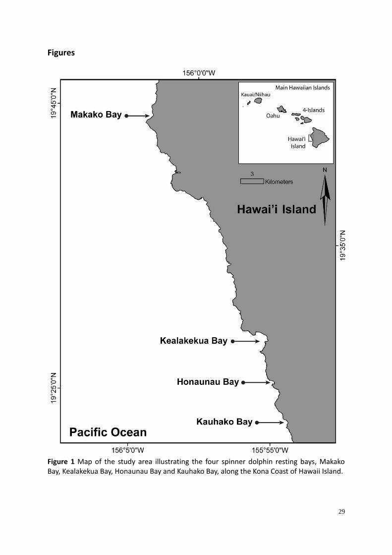
Hawaii Island is the largest, youngest and most southerly of the main Hawaiian Islands. On

the leeward (west) side of the island is the Kona Coast, where four important dolphin resting

bays are located: Makako Bay, Kealakekua Bay, Honaunau Bay and Kauhako Bay (Figure 1);

(Norris et al. 1994; Thorne et al. 2012; Tyne et al. 2014; Tyne et al. 2015).

2.2 Sampling design

Abundance estimated from data that have been collected opportunistically can increase the

risk of introducing sampling bias into the data, leading to inaccurate and imprecise

abundance estimates. To mitigate this risk from September 2010–August 2012, boat-based

photographic-identification was carried out in four important resting bays (Tyne et al. 2015)

of the Hawaii Island spinner dolphin stock using the systematic sampling design presented in

Tyne et al. (2014). Each bay was sampled on the same dates each month, regardless of

whether dolphins were present or absent, thus providing consistent and even effort

throughout the study period and area. This design, referred to as Scenario 1, consisted of 12

consecutive sampling days each month for each of the two years. Three additional sampling

regimes of reduced intensity (Scenarios 2, 3 and 4) were evaluated, using subsets of

Scenario 1 data, and compared with the results from Scenario 1. Finally, a fifth sampling

8

regime of a two-fold increase in sampling intensity from Scenario 1, i.e., 24 consecutive

sampling days each month, was also compared with the results from Scenario 1. Abundance

and precision were estimated for each year.

2.3 Sampling effort

The sampling effort in each of the five scenarios was:

Scenario 1 – 12 sampling days per month across four bays, two days in Makako Bay,

four days in Kealakekua Bay, two days in Honaunau Bay and four days in Kauhako Bay

(Figure 1).

Scenario 2 – six sampling days per month, spread across the four bays, with the days

chosen by randomly selecting half the number of days from each bay in Scenario 1.

Scenario 3 – six sampling days per month, across the two bays where dolphins were

encountered most frequently (two days in Makako Bay and four days in Kealakekua

Bay).

Scenario 4 – three sampling days per month, across two bays where dolphins were

encountered most frequently, with the days chosen by randomly sampling half the

number of days from each bay in Scenario 3 (one day in Makako Bay and two days in

Kealakekua Bay).

Scenario 5 – 24 sampling days per month across four bays chosen by randomly

selecting double the number of days from each bay in Scenario 1, four days in

Makako Bay, eight days in Kealakekua Bay, four days in Honaunau Bay and eight days

in Kauhako Bay.

9

2.4 Estimating costs

The relative costs of the different sampling regimes were estimated by determining the

number of hours required for field sampling and processing the images (including time to

score photographs for quality, animal distinctiveness, and propose putative matches

between photographic encounters) and multiplying this by an estimated labour costs of USD

$10. This cost was that of a technician/undergraduate student trained to complete the

tasks. In addition to labour costs, other costs are also associated with intensive boat-based

photo-identification studies, e.g., access to research boat, boat fuel and maintenance, car

fuel and maintenance, photo-identification equipment and computers.

2.5 Capture-recapture analysis

All photographs were graded according to photographic quality and distinctiveness to

minimise the introduction of bias and to reduce misidentification (Urian et al. 2015). Only

highly distinctive (D1) fins in photographs of excellent and good quality were included in the

capture-recapture analyses (Gowans and Whitehead 2001; Urian et al. 2015). A capture was

defined as a photograph of sufficient quality of an individual dolphin’s distinctly marked

dorsal fin. Capture histories corresponded to whether or not an individual dolphin was

“captured” or “recaptured” during a sampling occasion. This information was compiled for

each individual (calves excluded) after a photo-grading process. See Tyne et al. (2014) for

more details of the photo-grading process.

For both years, open and closed capture-recapture models in the program MARK (White and

Burnham 1999) were applied to the photo-identification data to estimate stock size,

variability and evaluate the goodness-of-fit of the models. See Tyne et al. (2014) for full

10

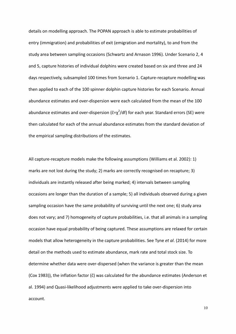
details on modelling approach. The POPAN approach is able to estimate probabilities of

entry (immigration) and probabilities of exit (emigration and mortality), to and from the

study area between sampling occasions (Schwartz and Arnason 1996). Under Scenario 2, 4

and 5, capture histories of individual dolphins were created based on six and three and 24

days respectively, subsampled 100 times from Scenario 1. Capture-recapture modelling was

then applied to each of the 100 spinner dolphin capture histories for each Scenario. Annual

abundance estimates and over-dispersion were each calculated from the mean of the 100

abundance estimates and over-dispersion (ĉ=χ2/df) for each year. Standard errors (SE) were

then calculated for each of the annual abundance estimates from the standard deviation of

the empirical sampling distributions of the estimates.

All capture-recapture models make the following assumptions (Williams et al. 2002): 1)

marks are not lost during the study; 2) marks are correctly recognised on recapture; 3)

individuals are instantly released after being marked; 4) intervals between sampling

occasions are longer than the duration of a sample; 5) all individuals observed during a given

sampling occasion have the same probability of surviving until the next one; 6) study area

does not vary; and 7) homogeneity of capture probabilities, i.e. that all animals in a sampling

occasion have equal probability of being captured. These assumptions are relaxed for certain

models that allow heterogeneity in the capture probabilities. See Tyne et al. (2014) for more

detail on the methods used to estimate abundance, mark rate and total stock size. To

determine whether data were over-dispersed (when the variance is greater than the mean

(Cox 1983)), the inflation factor (ĉ) was calculated for the abundance estimates (Anderson et

al. 1994) and Quasi-likelihood adjustments were applied to take over-dispersion into

account.

11

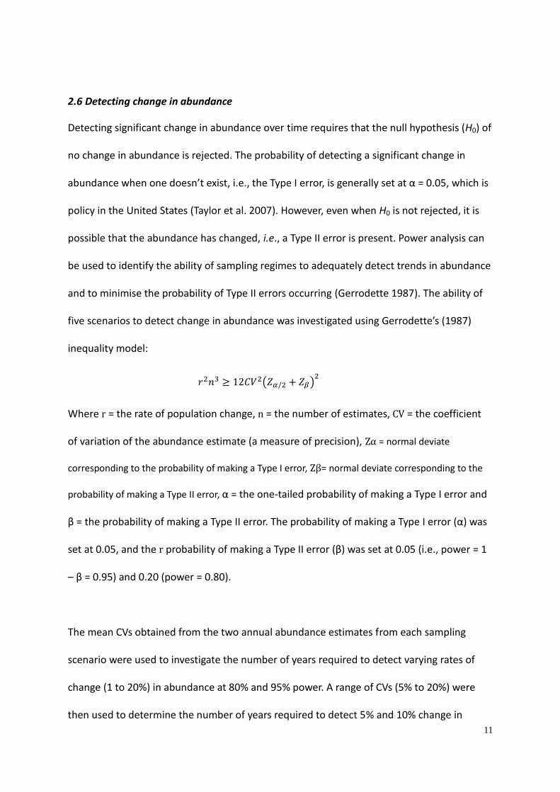
2.6 Detecting change in abundance

Detecting significant change in abundance over time requires that the null hypothesis (H0) of

no change in abundance is rejected. The probability of detecting a significant change in

abundance when one doesn’t exist, i.e., the Type I error, is generally set at α = 0.05, which is

policy in the United States (Taylor et al. 2007). However, even when H0 is not rejected, it is

possible that the abundance has changed, i.e., a Type II error is present. Power analysis can

be used to identify the ability of sampling regimes to adequately detect trends in abundance

and to minimise the probability of Type II errors occurring (Gerrodette 1987). The ability of

five scenarios to detect change in abundance was investigated using Gerrodette’s (1987)

inequality model:

Where r = the rate of population change, n = the number of estimates, CV = the coefficient

of variation of the abundance estimate (a measure of precision), Zα = normal deviate

corresponding to the probability of making a Type I error, Zβ= normal deviate corresponding to the

probability of making a Type II error, α = the one-tailed probability of making a Type I error and

β = the probability of making a Type II error. The probability of making a Type I error (α) was

set at 0.05, and the r probability of making a Type II error (β) was set at 0.05 (i.e., power = 1

– β = 0.95) and 0.20 (power = 0.80).

The mean CVs obtained from the two annual abundance estimates from each sampling

scenario were used to investigate the number of years required to detect varying rates of

change (1 to 20%) in abundance at 80% and 95% power. A range of CVs (5% to 20%) were

then used to determine the number of years required to detect 5% and 10% change in

𝑟2𝑛3 ≥ 12𝐶𝑉2(𝑍𝛼/2 + 𝑍𝛽)2

12

abundance at 80% and 95% power. Finally, we examined the number of years it would take

to detect a 5% change in abundance under the five scenarios.

3 Results

3.1 Effort and summary statistics

A total of 276 days (> 2,350 h of on-water effort) of photo-identification was carried out in

the four bays between September 2010 and August 2012. Approximately 4,000 h of effort

was required to identify and grade the individual spinner dolphins from the more than

200,000 images. More than 64,500 of these images were of sufficient quality to be added to

a photo-identification catalogue in which 235 individuals were classified as highly distinctive

individuals (D1). The identification of new individuals reached a plateau (90% of all

individuals identified) before the end of the two-year study period (August 2012, on

sampling day 276), with 211 dolphins (90%) identified after 114 sampling days (July 2011)

and 223 (95%) after 187 sampling days (February 2012, Figure 2).

3.2 Estimates of stock abundance

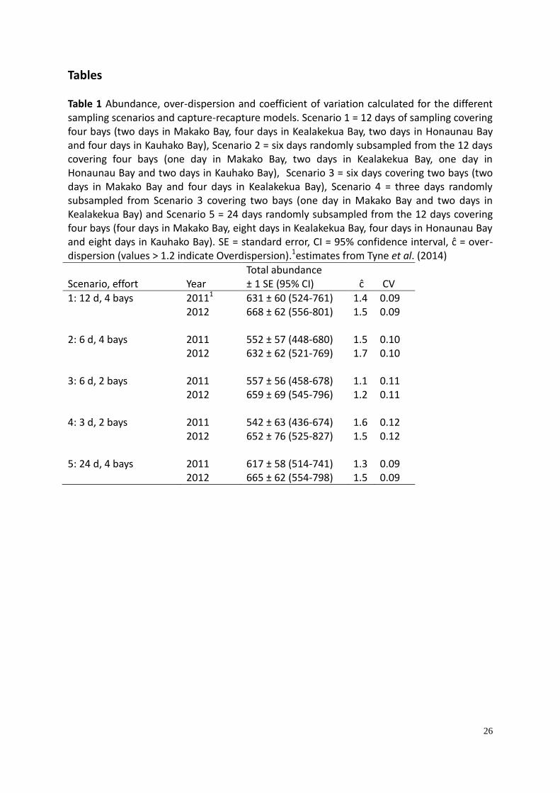
The abundance estimates were higher in 2012 than 2011 for all five scenarios. Although the

abundance estimates were more precise from Scenarios 1 and 5 (CV = 0.09), there was very

little difference in precision between the three scenarios (Scenarios 2, 3 and 4, CV = 0.10,

0.11 and 0.12 respectively). The goodness-of-fit measure (ĉ=χ2/df) suggested that the data

were over-dispersed for eight of the ten estimates (Scenarios 1, 2, 4 and 5) (Table 1).

3.3 Detecting change in abundance

The number of abundance estimates required to detect a change in the dolphin stock

decreased as the rate of change increased (Figure 3). For example, at a CV of 0.10 and a 5%

13

rate of change at 95% power, nine abundance estimates are needed to detect change,

compared with five abundance estimates to detect a 10% change (Figure 3). Furthermore, as

the precision decreased (i.e., CV increased), the time necessary to detect a change increased

(Figure 4).

The annual abundance estimates from the most intensive sampling Scenarios 1 and 5 were

the most precise (CV = 0.09; Table 2). Under these scenarios, it would take seven annual

abundance estimates over six years to detect a 5% annual change (decline/increase) with

80% power. Under the same scenarios with 95% power, it would take eight annual

abundance estimates over seven years to detect a 5 % change (Table 2). Under Scenario 4

(three field-days, two bays) and at 80% power, it would take eight annual abundance

estimates over seven years to detect a 5% change in abundance (Table 2). The annual labour

cost of Scenario 4 at 80% power was 27% that of Scenario 1 (12 field-days, four bays) at 80%

power (Table 2). As the time interval between abundance estimates increased from one to

three years, the number of abundance estimates required to detect a change decreased, but

the time taken to detect a change increased (Table 2). This is due to the increase in the

effective percentage change in abundance per interval (Gerrodette 1987; Wilson et al.

1999). To detect an annual 5% change at 80% and 95% power, it would take four and five

abundance estimates (at three year intervals), over nine and 12 years, respectively. If the

change was a continuous decline, the abundance would have declined by 37% and 46% by

the time of detection, equivalent to a decline from 668 ± 62 SE (95% CI 556-801) to 433 and

372. If the change in abundance was an increase, the abundance estimate would have

increased by 55% (1,035) and 80% (1,202) at the time of detection.

14

4 Discussion

This study aimed to provide a scientific basis for management agencies to develop

monitoring programs that are effective in fulfilling their statutory obligations, while also

providing information on where they might direct their scarce funding resources. To achieve

this aim, we estimated the abundance of Hawaii Island spinner dolphins in consecutive

years, modelled the ability of different sampling scenarios to detect change in abundance

over time and estimated the relative costs of these scenarios. Two main findings emerged

from this research. Firstly, the additional abundance estimates of the Hawaii Island spinner

dolphin stock were virtually identical to those from the first year (Tyne et al. 2014),

suggesting that the sampling design, developed to satisfy the assumptions of capture-

recapture models, is rigorous and that the estimates from the first year are reliable.

Secondly, although there was little difference in the precision between sampling scenarios,

sampling effort affected the ability of the sampling regime to detect a significant trend in

abundance over time. However, a point is reached where an increase in effort does not

improve the precision of the abundance estimates but that the costs of sampling continue to

increase (e.g., results from Scenarios 1 vs 5).

4.1 Estimates of abundance

The systematic sampling approach developed in Tyne et al. (2014) was designed specifically

to estimate the abundance of the Hawaii Island spinner dolphin stock using capture-

recapture models. Here, the data from this approach were used to evaluate the ability of five

different sampling scenarios to detect a change in abundance over time. The two most

intensive sampling scenarios, Scenarios 1 and 5 (Scenario 1 = 12 days each month in four

bays; Scenario 5 = 24 days each month, randomly resampled from Scenario 1, across four

15

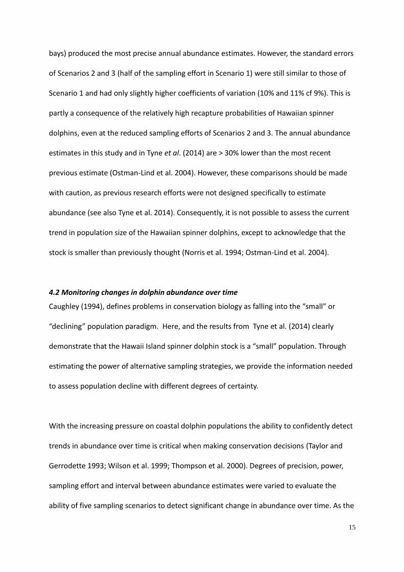
bays) produced the most precise annual abundance estimates. However, the standard errors

of Scenarios 2 and 3 (half of the sampling effort in Scenario 1) were still similar to those of

Scenario 1 and had only slightly higher coefficients of variation (10% and 11% cf 9%). This is

partly a consequence of the relatively high recapture probabilities of Hawaiian spinner

dolphins, even at the reduced sampling efforts of Scenarios 2 and 3. The annual abundance

estimates in this study and in Tyne et al. (2014) are > 30% lower than the most recent

previous estimate (Ostman-Lind et al. 2004). However, these comparisons should be made

with caution, as previous research efforts were not designed specifically to estimate

abundance (see also Tyne et al. 2014). Consequently, it is not possible to assess the current

trend in population size of the Hawaiian spinner dolphins, except to acknowledge that the

stock is smaller than previously thought (Norris et al. 1994; Ostman-Lind et al. 2004).

4.2 Monitoring changes in dolphin abundance over time

Caughley (1994), defines problems in conservation biology as falling into the “small” or

“declining” population paradigm. Here, and the results from Tyne et al. (2014) clearly

demonstrate that the Hawaii Island spinner dolphin stock is a “small” population. Through

estimating the power of alternative sampling strategies, we provide the information needed

to assess population decline with different degrees of certainty.

With the increasing pressure on coastal dolphin populations the ability to confidently detect

trends in abundance over time is critical when making conservation decisions (Taylor and

Gerrodette 1993; Wilson et al. 1999; Thompson et al. 2000). Degrees of precision, power,

sampling effort and interval between abundance estimates were varied to evaluate the

ability of five sampling scenarios to detect significant change in abundance over time. As the

16

sampling effort increased, so did the precision of the abundance estimates, and thus

changes in abundance could be detected earlier. This research provides the basis for

evaluating future trends in abundance as the current trend in population size is unknown,

and highlights the need for future systematic research designed to estimate abundance.

Clearly, the need for future estimates and evaluation of change in the Hawaii Island spinner

dolphin population size is a priority for managers because of the small population size (Tyne

et al. 2014), its genetic isolation (Andrews et al. 2010) and the use of the four bays

important for resting spinner dolphins (Tyne et al. 2015), where the dolphins encounter

significant numbers of human activities on a daily basis (Heenehan et al. 2015) .

4.3 Applications for monitoring

Hawaiian spinner dolphins are currently classed as a non-strategic stock under the MMPA

and under the current legislation, their abundance should be assessed once every three

years (Carretta et al. 2014). The NOAA are considering a management approach to reduce

the number and intensity of human-dolphin interactions in preferred resting habitat of

spinner dolphins, including the introduction of time-area closures of the four spinner

dolphin resting bays from this study (NOAA 2005). If time-area closures were introduced, a

monitoring program to detect trends in dolphin abundance would help evaluate the

effectiveness of this management strategy.

If the rate of change in abundance is small, then the level of precision will have a large effect

on the time needed to detect a change (Figure 3; see also Wilson et al. 1999; Thompson et

al. 2000; Taylor et al. 2007). The sampling effort for one of the most precise sampling

scenarios (1, CV = 9%) in this study required a significant investment of time and field

17

personnel and for the processing of the dolphin photo-identification images, and addition

costs for equipment and logistic expenses, e.g. boats, cars, cameras and housing. The

resources required for this research were only possible because of the presence of a

dedicated PhD student, large numbers of volunteer research assistants and significant

financial and logistical support through a NOAA grant. In general, the resources for

population monitoring programs are chronically underfunded (Williams and Thomas 2009;

Williams et al. 2011). Consequently, careful consideration on the distribution of funds for

resourcing population assessments is required in developing the sampling designs and

strategies for further estimates of the numbers in this spinner dolphin stock.

Management agencies can evaluate different monitoring options by comparing the different

scenarios investigated in this study, for example, an annual monitoring program

implemented under Scenario 4 (three field-days per month across two bays) is estimated to

require eight annual abundance estimates and take seven years to detect a significant 5%

change in abundance at 80% power. This is a year longer than the estimated time to detect

change using the annual monitoring program of Scenario 1 (12 field-days per month, across

four bays) at 80% power, a much more intensive sampling regime. If the change was

consistent decline in abundance, the spinner dolphin population would have reduced by

26% to 494 dolphins under Scenario 1 and by 30% to 468 dolphins under Scenario 4, before

a significant decline was detected. The annual cost of running a monitoring program

implemented under Scenario 4, however, is only 27% of the cost of the monitoring program

for Scenario 1. Furthermore, running an annual monitoring program implemented under

Scenario 2 (six field-days per month, across four bays), at 80% power, is estimated to require

18

seven surveys per year and take six years to detect a significant 5% change in abundance,

the same time required to detect a 5% change as Scenario 1 but at half the cost.

Other considerations in the design of the program include the rate of change in abundance

and the confidence of detecting significant change. By increasing power (confidence) to

detect a change, both the number of annual abundance estimates and study duration

required will increase (Gerrodette 1987; Taylor et al. 2007). The time taken to detect a

decline is critical for small, genetically isolated stocks, such as those of the Hawaii Island

spinner dolphins (Wilson et al. 1999; Thompson et al. 2000). A precipitous decline in

abundance will have significant, negative biological consequences for this spinner dolphin

stock. Consideration of these factors is a paramount concern, especially in determining the

level of precaution required to address management issues. Our findings suggest that

managers have an important decision to make: if current levels of monitoring are

inadequate to detect precipitous declines in a timely manner, is it appropriate to increase

monitoring efforts to improve statistical power or should a metric, other than population

decline, be used to trigger management intervention? The measures of precision for our

abundance estimates are enviably high (CVs of 9 to 11%) by the standards of even well-

monitored marine mammal stocks e.g., Cuvier’s beaked whale (Ziphius cavirostris) (CVs of 51

to 55%) (Moore and Barlow 2013), and managers in the region have other conservation

issues competing for scarce funding for research and mitigation efforts (Forney et al. 2011).

We see two, non-exclusive options for resolving the dilemma faced by managers: managers

could consider legal listing for spinner dolphins (i.e. classifying them as a strategic stock)

when the certainty of a decline is above 80%, rather than the conventional 95%; and/or

managers could act in a precautionary way and consider mitigation measures (e.g., time-

19

area closures) to mitigate impacts in hopes that population declines are prevented

altogether.

Another consideration in developing monitoring strategies for different cetacean species is

the proportion and distinctiveness of identifiable individuals in the population. For example,

Hectors dolphins (Cephalorhyncus hectori) have a low proportion of subtly distinctive

individuals, between 10%, (Gormley et al. 2005) and 35% (Bejder and Dawson 2001),

whereas in general, bottlenose dolphins (Tursiops spp.) have a larger proportion of highly

distinctive individuals of approximately e.g., 60%, (Wilson et al. 1999); 80%, (Nicholson et al.

2012). This spinner dolphin population had a relatively low proportion of distinctly marked

individuals (35%) (Tyne et al. 2014). Clearly, the distinctiveness of individuals has

implications for sampling precision and the ability of sampling programs to detect a change

in abundance.

These results provide a scientific basis for the level of precaution required to address

management issues, while assisting in the effective allocation of limited funding resources to

monitoring programs. The sampling design adopted by Tyne et al. (2014) and in the current

study to estimate the abundance of Hawaii spinner dolphins, when used in combination

with power analyses, can effectively determine when a trend in abundance will be detected

and should be considered as an integral part of any population management strategy. Here,

at the most intensive sampling scenarios we considered (Scenarios 1 and 5), with annual

surveys and abundance estimates assessed every three years at 95% power, the population

of spinner dolphins may have declined by 46% at the time a significant trend is detected.

This rate of decline is approximately 50% over 15 years, a rate that has been defined as

20

“precipitous” (Taylor et al. 2007) and could lead to the stock being classed as ‘depleted’

under the MMPA (Taylor et al. 2007). This is a serious concern for a small and genetically

isolated population, such as the one of Hawaii Island spinner dolphins. In order to be

consistent with the legislation within the MMPA, it will be necessary to increase funding for

monitoring or lower the burden of proof needed to trigger a change in classification from

non-depleted to depleted status.

We have shown little difference in the precision of abundance estimates between five

sampling scenarios of varying intensity but major differences in costs of the scenarios, with

the least intensive program costing about 30% of the scenario implemented by Tyne et al.

(2014) and 15% of the most intensive regime (Scenario 5 - 24 field-days per month, across

four bays). Management agencies can evaluate these different monitoring options while

considering the allocation of their available funding resources.

The objectives of population studies of other wildlife species with identifiable individuals

may require that demographic parameters other than abundance are estimated. Although

we have concentrated on the estimation of abundance and precision from different

scenarios, survival and immigration/emigration have also been estimated using the data

collected from this approach (Tyne et al. 2014). Delphinid sighting data have also been

collected systematically along transects to estimate abundance and other demographic

parameters, such as temporary immigration/emigration (Smith et al. 2013; Brown et al.

2016; Sprogis et al. 2016) using Pollock’s Robust Design (Pollock et al. 1990). The data from

these studies could be used to estimate the power to detect change and evaluate alternative

sampling strategies for monitoring in a similar manner to the current study by varying the

21

number of transect cycles. Using line transect sampling to estimate the abundance of

dolphins from a small boat, is not advisable however, as it can lead to biased estimates due

to the movement response of the dolphins towards and away from the boat prior to

detection (Turnock and Quinn 1991). The approach presented in the current study provides

a model for developing sampling strategies to monitor other populations with identifiable

individuals, including terrestrial and aquatic mammals (Pennycuick and Rudnai 1970; Wilson

et al. 1999), birds (Buckland et al. 2008; Williams and Thomson 2015) and reptiles (Sacchi et

al. 2010), whose abundance can be estimated through capture-recapture analyses.

22

Acknowledgements We would like to thank D.Kenison, J.Medeiros, the communities of Kealakekua, Ho’okena, Honaunau and Kailua Kona, L. van Atta, L. Smith, J. LeFors, J. Higgins and L. McCue for dialogue and support for this project. J. Vizbicke, S. Rickards, C. Gabriele, S. Yin, D. Perrine for help and equipment loan. We thank all the numerous fieldwork assistants who have helped on this project including A.Abe, D. Archambault, A. Archer, I. Baker, B. Banka, M. Battye, R. Blackburn, T. Boersch, L. Bray, A. Brossard, L. Ceyrac, S. Chan, M. Chapla-Hill, M. Chautard, L. Cunningham, A. Day, B. Dekker, S. Deventer, M. Durham, D.Fox, S.Gelibter, B. Gladden, S. Goecke, J.Goss, A. Greggor, D. Hanf, D. Hazel, H. Heenehan, L.Hoos, M. Howe, L. Ijsseldijk, R. Ingram, T. Johnson, S. Jones, C. Kulcsar, K. Lane, J. Loevenich, B. McKenna, K. New, K. Nicholson, K. Nikolich, M. O’Toole, N. Pendowski, S. Petrus, R. Reis, R. Smith, K. Sprogis, A. Steinkraus, J. Symons, M. ten-Doeschate, M. White, K. Wierucka, V. Wyss. We thank A. Read and G. Notarbartolo di Sciara for comments on a previous draft and two anonymous reviewers for constructive comments. Data were collected under the National Oceanic and Atmospheric Administration (NOAA) permit GA15409 and Murdoch University Animal Ethics Committee permit W2331/10. Funding was provided NOAA, The Marine Mammal Commission, Murdoch University and Dolphin Quest.

23

References

Anderson, D.R., Burnham, K.P., White, G.C., 1994. AIC model selection in overdispersed capture-recapture data. Ecology 75, 1780-1780.

Bejder, L., Dawson, S., 2001. Abundance, residency, and habitat utilisation of Hector's dolphins (Cephalorhynchus hectori) in Porpoise Bay, New Zealand. New Zealand Journal of Marine and Freshwater Research 35, 277-287.

Benoit-Bird, K.J., Au, W.W.L., 2009. Cooperative prey herding by the pelagic dolphin, Stenella longirostris. The Journal of the Acoustical Society of America 125, 125-137.

Brown, A.M., Bejder, L., Pollock, K.H., Allen, S.J., 2016. Site-specific assessments of the abundance of three inshore dolphin species to inform conservation and management. Frontiers in Marine Science 3.

Buckland, S.T., Marsden, S.J., Green, R.E., 2008. Estimating bird abundance: making methods work. Bird Conservation International 18, S91-S108.

Carretta, J.V., Oleson, E., Weller, D.W., Lang, A.R., Forney, K.A., Baker, J., M.M, M., Hanson, B., Orr, A.J., Huber, H., Lowry, M.S., Barlow, J., Moore, J.E., Lynch, D., Carswell, L., Brownwell Jr, R.L., 2014. U.S. Pacific Marine Mammal Stock Assessment: 2014. U.S. DEPARTMENT OF COMMERCE, National Oceanic and Atmospheric Administration, National Marine Fisheries Service, Southwest Fisheries Science Center., p. 406.

Caughley, G., 1994. Directions in Conservation Biology. Journal of Animal Ecology 63, 215-244.

Cox, D.R., 1983. Some remarks on overdispersion. Biometrika 70, 269-274. Forney, K.A., Kobayashi, D.R., Johnston, D.W., Marchetti, J.A., Marsik, M.G., 2011. What’s the

catch? Patterns of cetacean bycatch and depredation in Hawaii-based pelagic longline fisheries. Marine Ecology 32, 380-391.

Geffroy, B., Samia, D.S., Bessa, E., Blumstein, D.T., 2015. How Nature-Based Tourism Might Increase Prey Vulnerability to Predators. Trends in Ecology & Evolution.

Gerrodette, T., 1987. A Power Analysis for Detecting Trends. Ecology 68, 1364-1372. Gormley, A.M., Dawson, S.M., Slooten, E., Bräger, S., 2005. Capture-recapture estimates of

hector's dolphin abundance at Banks Peninsula, New Zealand. Marine Mammal Science 21, 204-216.

Gowans, S., Whitehead, H., 2001. Photographic identification of northern bottlenose whales (Hyperoodon Ampullatus): sources of heterogeneity from natural marks. Marine Mammal Science 17, 76-93.

Heenehan, H., Basurto, X., Bejder, L., Tyne, J., Higham, J.E.S., Johnston, D.W., 2015. Using Ostrom's common-pool resource theory to build toward an integrated ecosystem-based sustainable cetacean tourism system in Hawai`i. Journal of Sustainable Tourism 23, 536-556.

Higham, J.E.S., Bejder, L., Allen, S.J., Corkeron, P.J., Lusseau, D., 2016. Managing whale-watching as a non-lethal consumptive activity. Journal of Sustainable Tourism 24, 73-90.

Jaramillo-Legorreta, A., Rojas-Bracho, L., Brownell, R.L., Read, A.J., Reeves, R.R., Ralls, K., Taylor, B.L., 2007. Saving the Vaquita: Immediate Action, Not More Data. Conservation Biology 21, 1653-1655.

Kaschner, K., Quick, N.J., Jewell, R., Williams, R., Harris, C.M., 2012. Global Coverage of Cetacean Line-Transect Surveys: Status Quo, Data Gaps and Future Challenges. PLoS ONE 7, e44075.

Moore, J.E., Barlow, J.P., 2013. Declining Abundance of Beaked Whales (Family Ziphiidae) in the California Current Large Marine Ecosystem. PLoS ONE 8, e52770.

24

Nicholson, K., Bejder, L., Allen, S.J., Krützen, M., Pollock, K.H., 2012. Abundance, survival and temporary emigration of bottlenose dolphins (Tursiops sp.) off Useless Loop in the western gulf of Shark Bay, Western Australia. Marine and Freshwater Research 63, 1059-1068.

NOAA, 2005. Protecting spinner dolphins in the main Hawaiian Islands from human activities that cause ‘‘Take,’’ as defined in the Marine Mammal Protection Act and its implementing regulations, or to otherwise adversely affect the dolphins NOAA 051110296–5296–01; I.D.102405A.

Norris, K.S., Dohl, T.P., 1980. Behavior of the Hawaiian spinner dolphin, Stenella longirostris. Fish. Bull. 77, 821-849.

Norris, K.S., Wursig, B., Wells, S., Wursig, M., 1994. The Hawaiian Spinner Dolphin. University of California Press, Berkeley, CA.

Ostman-Lind, J., Driscoll-Lind, A., Rickards, S., 2004. Delphinid abundance, distribution and habitat use off the western coast of the island of Hawai'i. Administrative Report, p. 28. Southwest Fisheries Science Center

Parra, G.J., Corkeron, P.J., Marsh, H., 2006. Population sizes, site fidelity and residence patterns of Australian snubfin and Indo-Pacific humpback dolphins: Implications for conservation. Biological Conservation 129, 167-180.

Pennycuick, C.J., Rudnai, J., 1970. A method of identifying individual lions Panthera leo with an analysis of the reliability of identification. Journal of Zoology 160, 497-508.

Pollock, K.H., Nichols, J.D., Brownie, C., Hines, J.E., 1990. Statistical inference for capture-recapture experiments. Wildlife Monographs 107, 1-97.

Sacchi, R., Scali, S., Pellitteri-Rosa, D., Pupin, F., Gentilli, A., Tettamanti, S., Cavigioli, L., Racina, L., Maiocchi, V., Galeotti, P., Fasola, M., 2010. Photographic identification in reptiles: a matter of scales. Amphibia-Reptilia 31, 489-502.

Schwartz, C.J., Arnason, A.N., 1996. A General Methodology for the Analysis of Capture-Recapture Experiments in Open Populations. Biometrics 52, 860-873.

Smith, H.C., Pollock, K., Waples, K., Bradley, S., Bejder, L., 2013. Use of the Robust Design to Estimate Seasonal Abundance and Demographic Parameters of a Coastal Bottlenose Dolphin (Tursiops aduncus) Population. PLoS ONE 8, e76574.

Sprogis, K.R.-A., Pollock, K.H., Raudino, H.C., Allen, S.J., Kopps, A.M., Manlik, O., Tyne, J.A., Bejder, L., 2016. Sex-specific patterns in abundance, temporary emigration and survival of Indo-Pacific bottlenose dolphins (Tursiops aduncus) in coastal and estuarine waters. Frontiers in Marine Science 3.

Tablado, Z., Jenni, L., 2015. Determinants of uncertainty in wildlife responses to human disturbance. Biological Reviews, n/a-n/a.

Taylor, B.L., Gerrodette, T., 1993. The Uses of Statistical Power in Conservation Biology: The Vaquita and Northern Spotted Owl. Conservation Biology 7, 489-500.

Taylor, B.L., Martinez, M., Gerrodette, T., Barlow, J., Hrovat, Y.N., 2007. Lessons from monitoring trends in abundance of marine mammals. Marine Mammal Science 23, 157-175.

Taylor, B.L., Wade, P.R., De Master, D.P., Barlow, J., 2000. Incorporating Uncertainty into Management Models for Marine Mammals. Conservation Biology 14, 1243-1252.

Thomas, L., Buckland, S.T., Rexstad, E.A., Laake, J.L., Strindberg, S., Hedley, S.L., Bishop, J.R.B., Marques, T.A., Burnham, K.P., 2010. Distance software: design and analysis of distance sampling surveys for estimating population size. Journal of Applied Ecology 47, 5-14.

25

Thompson, P.M., Wilson, B., Grellier, K., Hammond, P.S., 2000. Combining Power Analysis and Population Viability Analysis to Compare Traditional and Precautionary Approaches to Conservation of Coastal Cetaceans. Conservation Biology 14, 1253-1263.

Thorne, L.H., Johnston, D.W., Urban, D.L., Tyne, J., Bejder, L., Baird, R.W., Yin, S., Rickards, S.H., Deakos, M.H., Mobley, J.R., Jr., Pack, A.A., Chapla Hill, M., 2012. Predictive modeling of spinner dolphin (Stenella longirostris) resting habitat in the main Hawaiian Islands. PLoS ONE 7, e43167.

Turnock, B.J., Quinn, T.J., 1991. The Effect of Responsive Movement on Abundance Estimation Using Line Transect Sampling. Biometrics 47, 701-715.

Turvey, S.T., Pitman, R.L., Taylor, B.L., Barlow, J., Akamatsu, T., Barrett, L.A., Zhao, X., Reeves, R.R., Stewart, B.S., Wang, K., Wei, Z., Zhang, X., Pusser, L.T., Richlen, M., Brandon, J.R., Wang, D., 2007. First human-caused extinction of a cetacean species?

Tyne, J.A., Johnston, D.W., Rankin, R., Loneragan, N.R., Bejder, L., 2015. The importance of spinner dolphin (Stenella longirostris) resting habitat: Implications for management doi: 10.1111/1365-2664.12434. Journal of Applied Ecology 52, 621-630.

Tyne, J.A., Pollock, K.H., Johnston, D.W., Bejder, L., 2014. Abundance and Survival Rates of the Hawai’i Island Associated Spinner Dolphin (Stenella longirostris) Stock. PLoS ONE 9, e86132.

Urian, K., Gorgone, A., Read, A., Balmer, B., Wells, R.S., Berggren, P., Durban, J., Eguchi, T., Rayment, W., Hammond, P.S., 2015. Recommendations for photo-identification methods used in capture-recapture models with cetaceans. Marine Mammal Science 31, 298-321.

Wade, P.R., 1998. Calculating limits to the allowable human-caused mortality of cetaceans and pinnipeds. Marine Mammal Science 14, 1-37.

White, G.C., Burnham, K.P., 1999. Program MARK: survival estimation from populations of marked animals. Bird Study 46, S120-S139.

Williams, B.K., Nichols, J.D., Conroy, M.J., 2002. Analysis and management of animal populations. Academic Press.

Williams, E.R., Thomson, B., 2015. Improving population estimates of Glossy Black-Cockatoos (Calyptorhynchus lathami) using photo-identification. Emu 115, 360-367.

Williams, R., Hedley, S.L., Branch, T.A., Bravington, M.V., Zerbini, A.N., Findlay, K.P., 2011. Chilean Blue Whales as a Case Study to Illustrate Methods to Estimate Abundance and Evaluate Conservation Status of Rare Species. Conservation Biology 25, 526-535.

Williams, R., Thomas, L., 2009. Cost-effective abundance estimation of rare animals: Testing performance of small-boat surveys for killer whales in British Columbia. Biological Conservation 142, 1542-1547.

Wilson, B., Hammond, P.S., Thompson, P.M., 1999. Estimating size and assessing trends in a coastal bottlenose dolphin population. Ecological Applications 9, 288-300.

26

Tables Table 1 Abundance, over-dispersion and coefficient of variation calculated for the different sampling scenarios and capture-recapture models. Scenario 1 = 12 days of sampling covering four bays (two days in Makako Bay, four days in Kealakekua Bay, two days in Honaunau Bay and four days in Kauhako Bay), Scenario 2 = six days randomly subsampled from the 12 days covering four bays (one day in Makako Bay, two days in Kealakekua Bay, one day in Honaunau Bay and two days in Kauhako Bay), Scenario 3 = six days covering two bays (two days in Makako Bay and four days in Kealakekua Bay), Scenario 4 = three days randomly subsampled from Scenario 3 covering two bays (one day in Makako Bay and two days in Kealakekua Bay) and Scenario 5 = 24 days randomly subsampled from the 12 days covering four bays (four days in Makako Bay, eight days in Kealakekua Bay, four days in Honaunau Bay and eight days in Kauhako Bay). SE = standard error, CI = 95% confidence interval, ĉ = over-dispersion (values > 1.2 indicate Overdispersion).1estimates from Tyne et al. (2014)

Scenario, effort Year Total abundance ± 1 SE (95% CI) ĉ CV

1: 12 d, 4 bays 20111 631 ± 60 (524-761) 1.4 0.09 2012 668 ± 62 (556-801) 1.5 0.09

2: 6 d, 4 bays

2011 552 ± 57 (448-680) 1.5 0.10 2012 632 ± 62 (521-769) 1.7 0.10

3: 6 d, 2 bays 2011 557 ± 56 (458-678) 1.1 0.11

2012 659 ± 69 (545-796) 1.2 0.11 4: 3 d, 2 bays 2011 542 ± 63 (436-674) 1.6 0.12 2012 652 ± 76 (525-827) 1.5 0.12 5: 24 d, 4 bays 2011 617 ± 58 (514-741) 1.3 0.09 2012 665 ± 62 (554-798) 1.5 0.09

27

Table 2 Number of annual abundance estimates, effective percentage change, years to detection, total percentage change at detection, at varying degrees of precision, to detect an annual 5% change (decline/increase) in abundance between one, two and three year monitoring intervals and annual labour costs based on Scenario 1 = 12 days of sampling covering four bays (two days in Makako Bay, four days in Kealakekua Bay, two days in Honaunau Bay and four days in Kauhako Bay), Scenario 2 = six days randomly subsampled from the 12 days covering four bays (one day in Makako Bay, two days in Kealakekua Bay, one day in Honaunau Bay and two days in Kauhako Bay), Scenario 3 = six days covering two bays (two days in Makako Bay and four days in Kealakekua Bay), Scenario 4 = three days covering two bays (one day in Makako Bay and two days in Kealakekua Bay) and Scenario 5 = 24 days randomly repeated subsamples from the 12 days covering four bays (four days in Makako Bay, eight days in Kealakekua Bay, four days in Honaunau Bay and eight days in Kauhako Bay). Probability of a Type I Error (α = 0.05) and a Type II Error (1 – β = 0.95 and 1 – β = 0.80). CV = coefficient of variation. Annual labour costs = four people paid $US10/hr working nine hrs/day on the boat, and processing time based on 2000 hours/year from Scenario 1.

Power

CV

Monitoring interval (years)

(t)

Annual abundance estimates

(n)

Effective % decline per interval t (0.95t – 1)

Effective % increase per

interval t (1.05t – 1)

Years to detection

(t(n-1))

Total % decline at detection

(0.95t(n-1) – 1)

Total % increase at detection

(1.05t(n-1) – 1)

Annual labour cost

($US)

Scenario 1 0.80 0.09 1 7 -5.0 5.0 6 -26 34 50,240 0.09 2 5 -9.8 10.3 8 -34 48 41,600 0.09 3 4 -14.3 15.8 9 -37 55 37,280 0.95 0.09 1 8 -5.0 5.0 7 -30 41 54,560 0.09 2 6 -9.8 10.3 10 -40 63 45,920 0.09 3 5 -14.3 15.8 12 -46 80 41,600 Scenario 2 0.80 0.10 1 7 -5.0 5.0 6 -26 34 25,120 0.10 2 5 -9.8 10.3 8 -34 48 20,800 0.10 3 4 -14.3 15.8 9 -37 55 18,640 0.95 0.10 1 9 -5.0 5.0 8 -34 48 29,440 0.10 2 7 -9.8 10.3 12 -46 80 25,120 0.10 3 6 -14.3 15.8 15 -54 110 22,960 Scenario 3 0.80 0.11 1 8 -5.0 5.0 7 -30 41 27,280 0.11 2 6 -9.8 10.3 10 -40 63 22,960 0.11 3 5 -14.3 15.8 12 -46 80 20,800 0.95 0.11 1 9 -5.0 5.0 8 -34 48 29,440 0.11 2 7 -9.8 10.3 12 -46 80 25,120 0.11 3 6 -14.3 15.8 15 -54 110 22,960 Scenario 4 0.80 0.12 1 8 -5.0 5.0 7 -30 41 13,640 0.12 2 6 -9.8 10.3 10 -40 63 11,480 0.12 3 5 -14.3 15.8 12 -46 80 10,400 0.95 0.12 1 10 -5.0 5.0 9 -34 55 15,800 0.12 2 8 -9.8 10.3 14 -46 98 13,640

28

0.12 3 7 -14.3 15.8 18 -54 141 12,560 Scenario 5 0.80 0.09 1 7 -5.0 5.0 6 -26 34 100,480 0.09 2 5 -9.8 10.3 8 -34 48 83,200 0.09 3 4 -14.3 15.8 9 -37 55 74,560 0.95 0.09 1 8 -5.0 5.0 7 -30 41 109,120 0.09 2 6 -9.8 10.3 10 -40 63 91,840 0.09 3 5 -14.3 15.8 12 -46 80 83,200

29

Figures

Figure 1 Map of the study area illustrating the four spinner dolphin resting bays, Makako Bay, Kealakekua Bay, Honaunau Bay and Kauhako Bay, along the Kona Coast of Hawaii Island.

30

Figure 2 Cumulative discovery curve of highly distinctive (D1) spinner dolphins during 276 photographic identification sampling days from September 2010 to August 2012. Short, dashed, vertical lines indicate when 90% and 95% of the highly distinctive individuals had been identified. Long vertical dashed line indicates 12 months of sampling.

Figure 3 Number of annual abundance estimates required to detect various rates of change in stock size at varying levels of precision (coefficient of variation, CV) from five sampling scenarios. Scenario 1 (S1) = 12 days of sampling covering four bays (two days in Makako Bay, four days in Kealakekua Bay, two days in Honaunau Bay and four days in Kauhako Bay), Scenario 2 (S2) = six days randomly subsampled from the 12 days covering four bays (one day in Makako Bay, two days in Kealakekua Bay, one day in Honaunau Bay and two days in Kauhako Bay), Scenario 3 (S3) = six days covering two bays (two days in Makako Bay and four days in Kealakekua Bay), Scenario 4 (S4) = three days covering two bays (one day in Makako Bay and two days in Kealakekua Bay) Scenario 5 (S5) = 24 days randomly subsampled from the 12 days covering four bays (four days in Makako Bay, eight days in Kealakekua Bay, four days in Honaunau Bay and eight days in Kauhako Bay). Type I error (α) probabilities were set

31

at 0.05 and Type II error (β) probabilities were set at power = 1 – β = 0.95 (dark lines) and 1 – β = 0.80 (grey lines).

Figure 4 Predicted time it would take to detect an annual change of 5% and 10% with varying levels of precision (coefficient of variation, CV) using monitoring intervals of one year and three years. Type I error (α) probabilities were set at 0.05 and Type II error (β) probabilities were set at 0.20. Power = 1 – β = 0.80 (grey) and power = 1 – β = 0.95 (dark). Vertical lines indicate CV range from the five sampling scenarios.