nasa conference publication 2297 , nonlinear ! nasa … · nasa conference publication 2297...
TRANSCRIPT

NASA Conference Publication 2297
, ....Nonlinear! NASA-CP-2297 1984002361g i
StructuralAnalysis
L.
" • ,2 .1
': ",:.',_ ; 0;_. Vi'; _Z'.:_1_"
https://ntrs.nasa.gov/search.jsp?R=19840023618 2018-06-10T13:34:04+00:00Z

J LI 3 1176 00519 9097

NASA Conference Publication 2297
NonlinearStructuralAnalysis
Proceedingsof a workshopheld at NASA Lewis Research Center
Cleveland, OhioApril 19and 20, 1983
NI_ANational Aeronautics
and Space Administration
Scientific and TechnicalInformation Branch
1984

PREFACE
NASALewis Research Center developed and has been conducting research onan enlarged engine structures program since 1979. Development of advancedmethods of nonlinear structural analysis of engine components is a significantpart this enlarged engine structures program and is an integrated researcheffort involving Lewis, industry, and the university community.
A two-day workshop was held at Lewis Research Center on April 19 and 20,1983, to report recent progress in nonlinear structural analysis for enginestructures. The workshop was organized into three sessions as follows:Session I - New Concepts/Formulations, Session II - Algorithms/Convergence,and Session III - Inelastic Analysis and Interactive Elements.
Newconcepts/formulations include (1) the slave finite-element formula-tion for space and time where interpolation polynomials (amenable to explicitintegration) are used to express all variables entering the formulation overthe element domain, (2) new variational principles leading to new formulationsfor hybrid stress finite elements that possess ideal characteristics, such asminimum sensitivity to geometric distortion, minimum number of independentstress parameters, and rank sufficiency, (3) shear-deformed shell finiteelements for laminated composites based on the total Lagrangian descriptionaccounting for anisotropic material behavior, dynamic response, arbitrarylaminate configuration, and arbitrary ply properties, and (4) large-aspect-ratio finite elements for nonlinear shell-type structures analysis based on ahigher order "degenerated: shell element with nine nodes and accounting forelastic-plastic behavior.
Algorithms/convergence include (1) self-adaptive solution strategiesfocusing on alternative formulations for developing algorithms that avoid theneed for global updating and inversion, (2) element-by-element solution proce-dures where approximate factorization is considered for solving the largefinite-element equation systems that arise in nonlinear structural analyses,(3) automatic finite-element generators, where the use of VAXIMA (MACSIMAinVAX) is used to generate the equations that describe the finite-element formu-lation, and (4) convergence criteria considering the effects of underintegra-tion on the element approximations.
Inelastic analysis and interactive elements include (1) inelastic anddynamic fracture, focusing on large, dynamic crack propagation by developingmethods for new path-independent integrals, for generalized inelastic consti-tutive relations, and for new complementary energy approaches, (2) interactivefinite elements where novel methods are developed to describe the bearing/-support interaction for general engine structural dynamics analysis, (3) non-linear composite structures analysis applicable to high-temperature compositematerial behavior, and (4) three-dimensional inelastic analysis via boundaryintegral, concentrating on the development of discrete element analysis basedon boundary integral concepts having the potential for substantial computa-tional efficiency for local concentrations compared with traditional finite-element analysis.
iii

Collectively, the papers included in these proceedings are representativeof cutting-edge methodology in all three disciplines. The authors of thepapers are nationally and internationally recognized experts in their respec-tive areas. The reader should bear in mind that the papers describe researchin progress. Results and conclusions reported are subject to revision asadditional results become available. In any event, these results and conclu-sions are those of the respective authors and not of the U.S. Government.
As workshop coordinator, I would like to thank all the authors for pre-paring their papers on time as well as the attendees whose extensivecontributions to the workshop discussions helped make the workshop a verysuccessful technical information exchange forum. Finally, I thank all thosewho helped with the mechanics of organizing and conducting the workshop.
C. C. ChamisLewis Research CenterCleveland, Ohio
iv

CONTENTS
Page
SESSIONI - NEWCONCEPTS/FORMULATIONS
Slave Finite Elements: The Temporal Element Approach toNonlinear Analysis
Slade Gellen, Bell Aerospace Textron ................. 1New Variational Formulations of Hybrid Stress Elements
T. H. H. Pian, K. Sumihara, and D. Kang, Massachusetts Institute ofTechnology .............................. 17
A Shear Deformable Shell Element for Laminated CompositesW. C. Chao and J. N. Reddy, Virginia Polytechnic Instituteand State University ........................ 31
Nonlinear Finite Element Analysis of Shells with Large Aspect RatioT. Y. Chang and K. Sawamiphakdi, The Univeristy of Akron ...... 45
SESSIONII - ALGORITHMS/CONVERGENCE
Self-Adaptive Solution StrategiesJoseph Padovan, University of Akron ..... 55
Element-by-Element Solution Procedures for Nonlinear StructuralAnalysis
Thomas J. R. Hughes, James Winget, and Itzhak Levit, StanfordUniversity ................... 65
Automatic Finite Element Generators"
Paul _ Wang, Kent State University ......... 85Stabili_j and Convergence of Underintegrated Finite'Eiement"Approximations
J. Tinsley Oden, The University of Texas .............. 95
SESSIONIII - INELASTIC ANALYSISAND INTERACTIVEELEMENTS
Inelastic and Dynamic Fracture, and Stress AnalysesSatya N. Atluri Georgia Institute of Technology ......... 105
Interactive Finite Elements for General Engine Dynamics AnalysisMaurice L. Adams, Case Western Reserve University, Joseph Podovan andDemeter G. Fertis, The University of Akron ............. 119
Nonlinear Analysis for High-Temperature Composites -Turbine Blades/Vanes
Dale A. Hopkins and Christos C. Chamis, Lewis Research Center . . 131Three-Dimensional Stress Analysis Using the Boundary Element Method"
Raymond B. Wilson, Pratt & Whitney Aircraft, Prasanta K. Banerjee, "State University of New York .................... 149
SummaryChristos C. Chamis, Lewis Research Center .............. 161


SLAVE FINITE ELEMENTS: THE TEMPORAL ELEMENT
APPROACH TO NONLINEAR ANALYSIS*
Slade Gellin
Bell Aerospace Textron
SUMMARY
A formulation method for finite elements in space and time incorporating non-linear geometric and material behavior is presented. The method uses interpolationpolynomials for approximating the behavior of various quantities over the element
domain, and only explicit integration over space and time. While applications are
general, the plate and shell elements that are currently being programmed will beused to model turbine blades, vanes and cumbustor liners.
INTRODUCTION
The extension of the finite element method to the solution of transient field
problems by discretizing in time as well as in space has been investigated in the
last fifteen years. The works most often cited are those byArgyris and Scharpf(Ref. i) and Fried (Ref. 2). The starting point of their work was Hamilton's
principle. Generally, sample problems consisted of axial thrust members, and only
linear geometric and material properties were assumed. There were some arbitrary
decisions made concerning the proper use of the initial conditions in the global
system in order to derive the correct set of equations for the given problem. Manyof the theoretical fine points were explained by Simkins (Ref. 3), who demonstrated
his findings using point mass structures. His results indicated that very highlevels of accuracy can be obtained with only a very small number of elements. He
notes that the temporal elements are well suited to handle sudden changes in load
function, extending the interval of solution indefinitely without restart, andproviding great detail to the solution in any subinterval. Furthenaore, conven-
tional step-by-step integration algorithms may call for a large number of time
steps, particularly for the hyperbolic equations of structural dynamics should the
excitation or material properties change rapidly in time. It is within this spiritthat this research was undertaken.
During the course of this work it was found that many theoretical questionsneeded to be answered. Some of these questions have deep physical and mathematical
importance, others are exercises in intellectual gamesmanship. Hopefully, they will
be addressed in forth-coming papers. The focus here will be on incorporating non-linear geometric and material behavior into the temporal element approach, within
the framework of the ground rules discussed in the following paragraphs.
*This work was performed under NASA Contract No. NAS3-23279.

First, the elements will be of what will be referred to as the "prismatic"
type. The space time domain is thought of as a long, prismatic, member in four
dimensions, with the "length" dimension corresponding to time. The three dimen-sional "cross-section" is the spatial model of the structure. A prismatic element
consists of the space-time domain occupied by a spatial finite element from t=t i
to t=tj. Geometrically, this is a well defined set of "longitudinal fibers" overa certain "length". A set of local coordinates is chosen with the time direction
the same as global time, but translated so that the time interval goes from 0 to
T=tj-t i. See Figure i.
Second, all field quantities will either be derived from the displacement
field directly or calculated at grid points and then interpolated with their own
shape functions over the space-time domain. This will facilitate the explicit
integration that also will be required for the procedure. Note that certain
spatial geometries for the element may require special handling. Isoparametric
representation of elements may not be desirable as only numerical integrationschemes will generally be feasible.
Finally, it will be assumed that the constitutive laws will be linear be-tween the time derivatives of the appropriate kinematical and dynamical quantities.
Some linearization must be available in order for the matrix techniques of finite
element analysis to be applicable.
The non-linear algorithm is derived in the following section. In the sub-
sequent section, a simple, but purposely poorly constructed example conducive to
hand computation is presented. Finally, some brief comments about the current
research being done using the temporal element concept will be given.
Non-Linear Algorithm
Like most non-linear algorithms, the one presented here is based on an
iterative procedure involving quasi-linearization. The difference in philosophy
between the method presented here and the conventional step-by-step methods, such
as the tangent modulus or residual force methods, is demonstrated graphically in
Figure 2. In both Figures 2(a) and 2(b), the heavily drawn curve represents the"exact" time history of quantity A, which may be thought of as the displacement
of a certain point, or a stress at a point, etc. In Figure 2(a), the step-by-step
method has calculated the path OA, representing the history up to that point. At
A, the procedure generates successive approximations ABi until convergence to the
path AB is achieved. The procedure is now repeated at B. For the algorithm
presented here, Figure 2(b) indicates that successive iterations generate an
entire load history. This load history allows for determining loading and unloading
paths for the entire time interval of interest, eliminating the guesswork or sub-
interval changes usually associated with the step-by-step methods. Iterations
converge until the curve OC is obtained.
The theoretical basis for the algorithm is Hamilton's law of varying action.
Essentially, it is the principle of virtual work integrated over time. It is
expressed mathematically as
T .... }T{F_}__ f (_'0 - 6v " p) dVdt - {_u = 0 (i)ui V
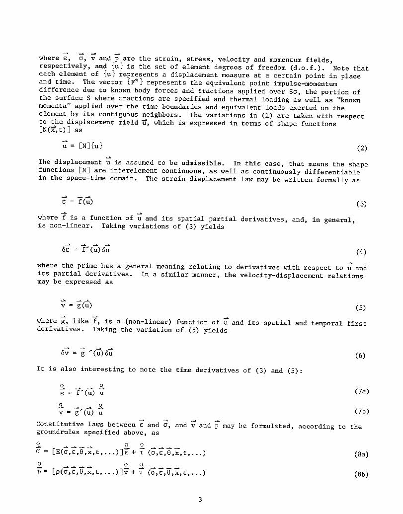
where g, _, v and p are the strain, stress, velocity and momentum fields,
respectively, and {u} is the set of element degrees of freedom (d.o.f.). Note that
each element of {u} represents a displacement measure at a certain point in place
and time. The vector {F*} represents the equivalent point impulse-m_mentum
difference due to known body forces and tractions applied over S_, the portion of
the surface S where tractions are specified and thermal loading as well as "known
momenta" applied over the time boundaries and equivalent loads exerted on the
element by its contiguous neighbors. The variations in (i) are taken with respect
to the displacement field_, which is expressed in terms of shape functions
[N_,t)] as
u = [N]{u} (2)
The displacement u is assumed to be admissible. In this case, that means the shape
functions IN] are interelement continuous, as well as continuously differentiable
in the space-time domain. The strain-displacement law may be written formally as
= f(u) (3)
where f is a function of u and its spatial partial derivatives, and, in general,
is non-linear. Taking variations of (3) yields
6_ = f'(u)6u (4)
where the prime has a general meaning relating to derivatives with respect to u and
its partial derivatives. In a similar manner, the velocity-displacement relations
may be expressed as
v = g(u) (5)
where g, like f, is a (non-linear) function of u and its spatial and temporal first
derivatives. Taking the variation of (5) yields
_v = g "(u)_u (6)
It is also interesting to note the time derivatives of (3) and (5):
O O........... (7a)€ = f'(u) u
v = g (u) u (7b)
Constitutive laws between g and _, and v and p may be formulated, according to the
groundrules specified above, as
o o o
O = [E , ,_,x,t,...) + T (O,g,@,x,t,...) (8a)
O O u
p = [p(_,g,@,x,t,...)]_+ _ (d,_,@,x,t,...) (8b)

where O is the temperature field. Equations (8) are integrated from 0 to t; thus,
t O
= / _ dt" + _ (9a)o o
t o
p = f p dt" + Po (9b)o
where o and p are the values of the stress and momentum at local time t=0. Theseo o
may be approximated by
L = [N_(_)]_o} (10a)
= NpPo [ (x)_Po } (10b)
where the number of parameters in {oo} and {po } is arbitrary. Ideally, [No] isinterelement continuous, and both [N_] and [ND] are as sophisticated as the stressand momentum fields derived from [N] in the linear theory, though neither require-
ment is really mandatory.
In the iterative procedure to be used, "current" values of displacement,
stress, strain, etc., for the entire load history are in hand. These values are. __. o . -_ are calculated
used to evaluate ]_ , g , [E], _, [0] and o__ The quantities _ and ofrom (2) where the set {u} are unknown, _representing the "updated"Usolution.
Similarly, {go}and {Po } are unknowns.
Equations (3)-(7) may be re-expressed as
6__= [f'][N]{6u} (lla)O
= [f'][N] {u} (llb)
6v = [g'][N]{_u} (llc)
O
v = [g'][N]{u} (lld)
where If'] and [g'] are 6x3 and 3x3 operator matrices, respectively. Stress andmomentum matrices are defined by
t o
Es] = f EE]Ef'][N]dt" (12a)°t o
[M] = f [p]Eg'][N] dt" (12b)O
and stress and momentum vectors are defined as
to
T = f T dt" (13a)o
___ t °
= f _dt" (13b)o
4

Using (i0), (12) and (13) in (9) yields
O = [S]{u} + • + [No]{O o} (14a)
p = [M]{u} + _ + [Np]{p o} (14b)
Equations (14) may be evaluated at t=T. (Quantities evaluated at this time are
given a T subscript.) Assuming that [No] and [Np] can also approximate °T and _T'equations (14) take on the form
[ST]{U} + Tr + [NO] {(_o-aT} = {0} (15a)
[MT]{U} ":-rf-_T+ [Np] {po-PT } = {0} (15b)
at t=T. Equations (15) are used as subsidiary conditions to the problem. They
are added to (i) with the use of lagrange multiplier fields. In particular, the
choices for the stress and momentum fields, respectively, is given as
= NO 10I(7 [ ]{ } (16a)
Ip = [Np]{kp} (16b)
These fields are used with (15) and integrated over the volume. These conditions,
as well as equations (lla), (llc), and (14) are used in (i) to give
{_u}T([Ke]{U} - {F*} - {F_}-{F_}+[A_]{(7O} - [Ap]{Po})
e
+ _({%O} T([B_]{u} + [Co]{(7o-OT} - {q_} )
+{kp}T'rBel[p]{U} + [Cp]{po-PT} - {q_}) = 0 (17)
whereT
[Ke] = °f vf ([N]T[f']T[s] - [N] T[g']T[M] ) dVdt (18a)
T
[A_] = °f vf [N]T[f']T[No]dVdt (18b)
T
lAp] = _ vf [N]T[g']T[Np]dVdt (18c)
[B_] = vf [No]TEST]dV (18d)

[Bp] = v/ ENp]T[MT]dV (18e)
[C$] = $ [N_]T[No]dV (18f)
[C_] = _ [Np]r[Np]dV (igg)
T
L f[N]r[f']r{F } = - T dVdt (18h)
v
T
{q_} = - _No]T _TdV (iSj)v
{q_} = - v_Np]T gTdV (iSk)
The set of equations generated by (17) when variations are taken on {u}, {go },
{Po}, {IO } and {Ip} are T T
[Ke]{U} + [A_]{Oo} - [A_]{po}+[B_] {_} + [Bp] {%p}
= {F*}+ {F_}+ {F$} (19a)
[C_]{%_} = {0} (19b)
[Ce] {_ } = {0} (19c)P P
Ce[B_]{u} + [ O]{Oo-OT } = {q_} (19d)
e
[Bp]{U} + [c_e]{po-pT}p = {q_} (19e)
Note that the matrices _C_] and e[Cp_will be square and invertible, thus makingthe mulipliers identically zero. They may then be omitted from equation (19a).
Equations (19a, d, e) are assembled into the systems
[K]{u} + [A ]{_} - [Ap]{p} = {P} (20a)
[B ]{u} + [C ]{_} = {qy} (20b)
[Bp]{U} + [Cp]{Po} = {q_} (20c)

where the assembly enforces the conditions of continuity across a time boundaryfor stress and continuity of momentum across a time boundary to the extent that no
impulses per unit volume are applied, and, if such impulses are implied, an
appropriate discontinuity is maintained. The results should leave [C_] and [C ]square and invertible. Thus, equations (20b,c) are solved for {_} and {p} and_used in (20a) to derive the global stiffness equations
A A
[K]{u} = {P} (21)
where
[K] = [K] - [A ] [C ]-lIB ] + [Ap][Cp]-l[Bp] (22a)
[P] = [>] - [AO] [Co]-l[q T] + [Ap][Cp]-l[q_] (22b)
Equations (21) are solved for {u} and then back-substituted into all the pertinentequations to calculate the important quantities to be used in the next iteration.
A Simple Numerical Example
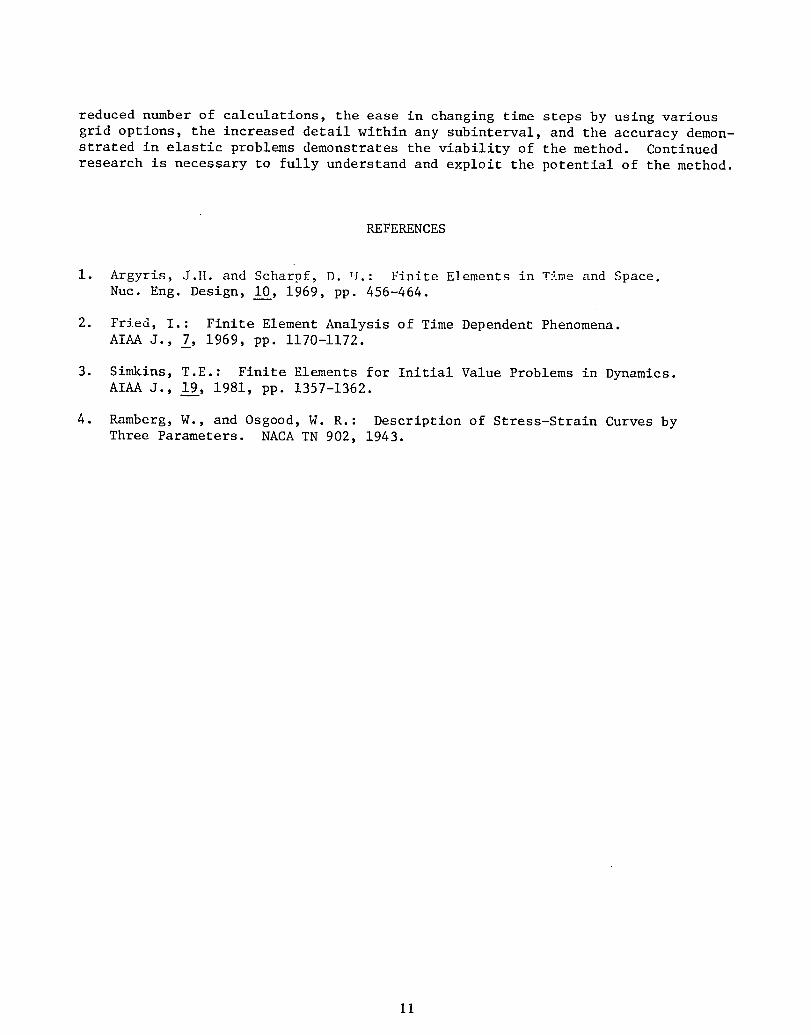
To demonstrate some of the procedures developed, a numerical example willbe worked out. A rod of length L, and cross-sectional area A built in at both
ends, is loaded at its midpoint by a continuously time varying load p(t) given as
P(t) = 2_ A(t )y _ (23)
where T is the time interval of interest and _y is the nominal yield stress of the
material satisfying the uniaxial stress strain law of the Ramberg-Osgood type(Reference 4)
_ [i + 3 (_y) 8= _ _ ] (24)
where E is the elastic modulus of the material. The loading is assumed quasistatic
and thus dynamic effects may be ignored. (Note that if P(t) is discontinuous,
dynamic effects must be introduced in order to maintain continuity of displacement
and stress across a time boundary.) The rod is initially in the undeformed state;thus, not only is u(x,0)=0, but _(x,0)=0. See Figure 3.
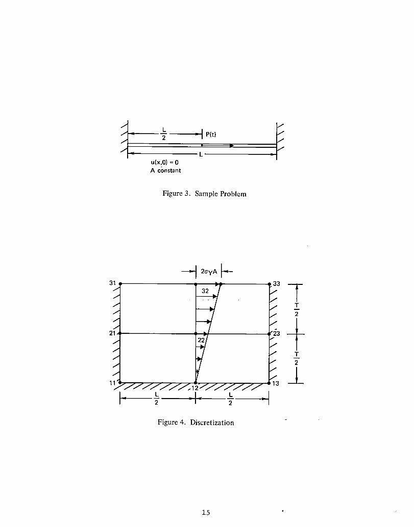
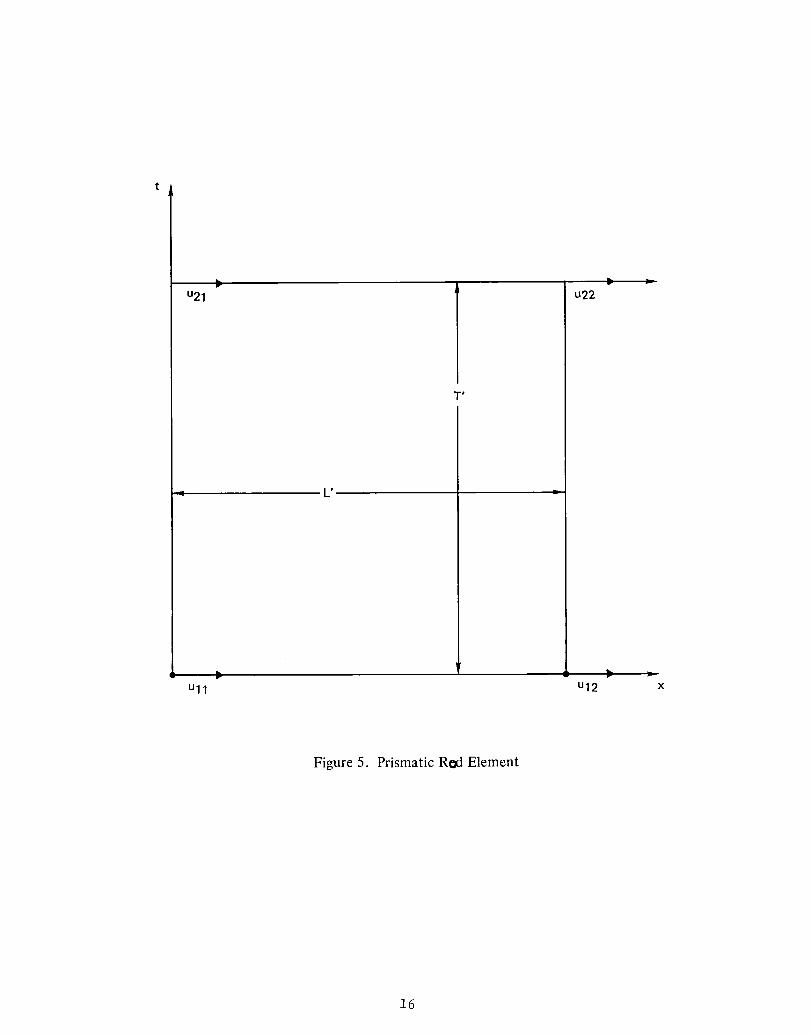
The problem is discretized using four elements, each of dimensions L/2 byT/2, as seen in Figure 4. Each element is of the type shown in Figure 5. The
displacement field for this element is modeled using the bilinear shape functions
, , e ,)e (l-x/L)(1-t/T )+u21 (I-x/L (t/r')u(x, t)=Ull
e (x/L') (l-t/r' e ,)+ u12 )+u22 (x/L')(t/r (25)
7
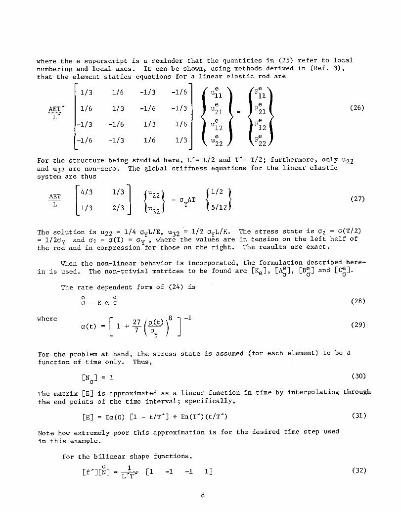
where the e superscript is a reminder that the quantities in (25) refer to local
numbering and local axes. It can be shown, using methods derived in (Ref. 3),
that the element statics equations for a linear elastic rod are
" e _ _
AET" 1/6 1/3 -i/6 -i/3 F21 (26)
L" e
-1/3 -1/6 1/3 1/6 u12 IF121
-1/6 -1/3 1/6 1/3 u22 _kF22)
For the structure being studied here, L"= L/2 and T'= T/2; furthermore, only u22
and u32 are non-zero. The global stiffness equations for the linear elasticsystem are thus
AET 4/3 1/3 u22 = OyAT (27)L 1/3 2/3 [u32 5/12
The solution is u22 = 1/40yL/E, u32 _ 1/2 _yL/E. The stress state is _2 = O(T/2)
= i/2_y and _s = _(T) = _y , where the values are in tension on the left half ofthe rod and in compression for those on the right. The results are exact.
When the non-linear behavior is incorporated, the formulation described here-
in is used. The non-trivial matrices to be found are [Ke] , [A_], [B_] and [C_].
The rate dependent form of (24) is
O O
O = E _ g (28)
w ere[For the problem at hand, the stress state is assumed (for each element) to be afunction of time only. Thus,
[N ] = i (30)
The matrix [E] is approximated as a linear function in time by interpolating through
the end points of the time interval; specifically,
[E] = KS(0) [i - t/T'] + E_(T')(t/T') (31)
Note how extremely poor this approximation is for the desired time step used
in this example.
For the bilinear shape functions,
o 1[f'][N]= El -1 -1 i] (32)L'T"
8
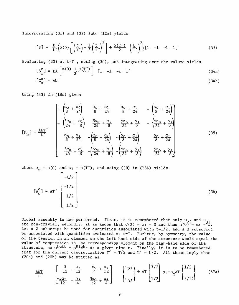
Incorporating (31) and (32) into (12a) yields
Es]= E T" * ,El-1-1 i] (33)
Evaluating (33) at t=T , noting (30), and integrating over the volume yields
[B_] = EA [_(0) +2 C_(T')] [1 -1 -1 1] (34a)
Ece] = AL" (34b)
Using (33) in (18a) gives
+ el ._o e_JL eo +__ _ + e8 + 24 8 24
_ (_# +_) 5_o24+ _18 5_o24+ 8-_I _ (52_+_
[Ke] - AET" (_ -i4)
_5_o24+_ -(@+_) -(_4°+_) 5_--°+_24
where s° = _(0) and _l = _(T'), and using (30) in (18b) yields
-i/2
-1/2
[A_] = AT" (36)u
1/2
1/2
Global assembly is now performed. First, it is remembered that only u22 andare non-trivial; secondly, it is known that _(0) = _I = 0 and thus _(07 = _I u?=31.
Let a 2 subscript be used for quantities associated with t=T/2, and a 3 subscript
be associated with quantities evaluated at t=T. Furhter, by symmetry, the valueof the tension in an element on the left hand side of the structure would equal the
value of compression in the corresponding element on the righ-hand side of the
structure, so _Left = aRight at a given time t. Finally, it is to be remembered
that for the current discretization T" = T/2 and L" = L/2. All these imply that(20a) and (20b) may be written as
AET 12 -4- _ Iu22 t + AT _2=OyAT _ (37a)
4 12

EA(I + _2)[ 1 0 ] Iu22 1 AL2 u32 - _- _2 = 0 (37b)
Solving (37b) for 02 and using the results in (37a) yields the global stiffness
equat ions
° ° I I_2 _ _3 ] 1/2
_+ 2 12 4 - 12 u22
AET = OyAT _ (38)
L + _2 _3 5_2 + _j [ u32 _5/1212 4 12 4J
Note that if the structure is considered linear elastic that _2 = _3 = I, and
equations (38) become identical to the elastic global equations (27).
Equations (38) were solved iteratively for u22 , uR?, 02 and 03 using ahand-held calculator maintaining four-place accuracy in_he coefficients of thestiffness matrix. Table 1 lists the results of each iteration where the elastic
case is taken as the initial condition. It should be noted that the trend indi-
cated by the table implies that greater accuracy must be retained to achieve con-
vergence; however, three place accuracy is reached rather quickly. The results
are not bad when considering the absolutely horrendous approximations used in the
example. It is concluded that the general method is viable.
Related Research
As noted in the introduction, there were many theoretical questions which
were needed to be answered that arose during the course of this study. Many of the
questions concerning the incorporation of the initial conditions to the transient
problem into a formulation that is inherently suited to boundary type conditions
were answered both independently and through (ref. 3). There were other questions
concerning non-prismatic or semi-prismatic discretizations, and their possible use
in both formulating elements and in modeling specific problems in space and time.
Several modified or hybrid variational formulations were developed to model ele-
ments possessing certain qualities, such as an embedded hole or non-rectangular
geometry for grid elements, where interelement continuity would be more difficult
to maintain. A search for a four-dimensional, unified theory for elastic dynamicsolid mechanics was undertaken in order to better understand the parallel conditions
that must exist between the spatial and temporal properties of a structure. Not to
be overlooked are the various computer programming difficulties, particularly the
large numbers of d.o.f, per element that could be generated for elements of this
type, and the adaptability of element modules with a solution procedure provided
by another host program.
CONCLUDING REMARKS
The Slave Finite Element approach to non-linear analysis has been presented.
Despite the large number of dof in the system for any given problem, the anticipated
I0
reduced number of calculations, the ease in changing time steps by using various
grid options, the increased detail within any subinterval, and the accuracy demon-
strated in elastic problems demonstrates the viability of the method. Continued
research is necessary to fully understand and exploit the potential of the method.
REFERENCES
1. Argyris, J.ll. and Scharpf, D.U.: Finite Elements in Time and Space.
Nuc. Eng. Design, i0, 1969, pp. 456-464.
2. Fried, I.: Finite Element Analysis of Time Dependent Phenomena.
AIAA J., _, 1969, pp. 1170-1172.
3. Simkins, T.E.: Finite Elements for Initial Value Problems in Dynamics.
AIAA J., 19, 1981, pp. 1357-1362.
4. Ramberg, W., and Osgood, W. R.: Description of Stress-Strain Curves byThree Parameters. NACA TN 902, 1943.
II

TABLE i: NUMERICAL COMPUTATIONS FOR SAMPLE PROBLEM
Iteration # u22E/OyL u3eElOyL o2/ y o3/oy0 .2500 .5000 5000 1.0000 .9852 .2059
1 .2409 .6252 4782 .9359 .9896 .3058
2 .2423 .6016 4821 .9475 .9889 .2853
3 .2420 .6061 4813 .9452 .9890 .2892
4 .2420 .6053 4813 .9457 .9890 .2884
5 .2420 .6054 4813 .9457 .9890 .2887
(no further change in stiffness matrix)
EXACT .2504 .7143 .5000 1.0000
% ERROR 3.4 15.3 3.7 5.5

t t
mm
J
t _ Y'
Y X'×
Figure 1. Two Dimensional Prismatic Element
13

z_
ByI III I _ to
(a)
C1/
/ C
//
//
/0 _ t
(b)
Figure 2. Comparison of Non-Linear Algorithms (a) Step-By-Step Method(b) Slave Finite Element Method
14
L ,=- P(t)2 I
I- L -Iu(x,0) = 0A constant
Figure 3. Sample Problem
-_ 2ayA
_ / T
J
21- j37- J/ 7 T
/ 711" _13
2 2
Figure 4. Discretization
15
u21 u22
T t
,,i L °
i
; • .=Ull u12 x
Figure 5. Prismatic Rod Element
16
NEWVARIATIONALFORMULATIONSOF HYBRIDSTRESSELEMENTS*
T.H.H. Pian,t K. Sumihara tt and D. KangttMassachusetts Institute of Technology
SUMMARY
In the variational formulations of finite elements by the Hu-Washizu andHellinger-Reissner principles the stress equilibrium condition can be maintainedby the inclusion of internal displacements which function as the Lagrange multi-pliers for the constraints. These new versions permit the use of natural coordi-nates and the relaxation of the equilibrium conditions and, render considerableimprovements in the assumed stress hybrid elements. These include the derivationof invariant hybrid elements which possess the ideal qualities such as minimumsensitivity to geometric distortions, minimum number of independent stress param-eters, rank sufficient and ability to represent constant strain-states and bendingmoments. Another application is the formulation of semiLoof thin shell elementswhich can yield excellent results for many severe test cases because the rigidbody nodes, the momentless membrane strains and the inextensional bending modescan all be represented.
INTRODUCTION
In the original formulation of the assumed stress hybrid elements by themodified complementary energy principle (ref. I) and the later extension usingthe Hellinger-Reissner (ref. 2) the assumed stress are made to satisfy the equilib-rium equations a priori. This restricts the derivation to the use of physicalcoordinates such as Cartesian coordinates and shell surface coordinates, etc. andto the coupling of the various stress components by the equilibrium equations.Such restrictions are the chief obstacles for the construction of shell elementsby the hybrid method and the main reasons why the element properties often deterio-rate rapidly when unfavorable reference coordinates are used for stresses and/orwhen the element geometry is distorted.
Recently new versions of the Hellinger-Reissner and the Hu-Washizu principleshave been suggested for more efficient formulations of hybrid stress elements(refs. 3 and 4). This paper presents two specific applications of these principles:(I) the formulation of invariant hybrid stress elements by the Hellinger-Reissnerprinciple and (2) the derivation of semiLoof shell elements by the Hu-Washizuprinciple.
The research reported here is one part of a program the objective of whichis to advance the numerical tools for analyzing engine structures which needs tobe modelled by 3-D solids and/or shell structures.
The work was sponsored by the NASALewis Research Center under NASAGrantNo. NAG3-33.
tprofessor of Aeronautics and Astronautics
ttGraduate Student
17

FORMULATIONOF INVARIANTHYBRIDSTRESSELEMENTS
The modified version of the Hellinger-Reissner principle for the formulationof the element stiffness matrix may be stated as
_R = f [-½ _TS _ + _T(D Uq) - (DTo)T ul]dV : Stationary (I)
where _ = stress, S = elastic compliance, V = element volume, uq = elementdisplacements that a_e interpolated compatibly in terms of nodal dlsplacements qand u_, = additional internal displacements which are expressed in terms of para_e-tars ~ I that can be statically condensed. Here
(DT_) = 0 (2)
is the equation of equilibrium. Hence the last term in the functional plays therole of conditions of constraint with the corresponding Lagrange multipliers. Thus,the assumed stresses _ need not be coupled initially and the introduction of dis-placement parameters _ will reduce the number of independent stress parameters.
As an example, the derivation of the quadrilateral membrane element ispresented. Here, for the o stresses, the nine terms are complete in linear termsin the natural or isoparam_tric coordinates _, n,
o : Oy : I _]q " (3)
T _q B9£ xy
The element displacements are interpolated by bilinear polynomials in thenatural coordinates. Here it is expected that in the limiting case of rectangularelements the present formulation should yield the 5-B hybrid stress element (ref. 5)that is known to have excellent properties.
Thus, four internal displacement terms are need. They are, indeed, the sameones used by Wilson et al. (ref. 6) in their incompatible elements, i.e.
u_ = _i(I-_ 2) + _2(l-n 2) (4)v_ = X3(I-_2 ) + X4(l-n 2)
It is noted that these additional displacement terms are essential because they nowmake the displacements u complete in quadratic terms.
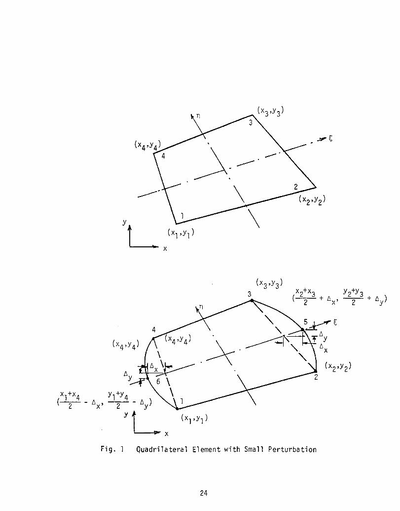
In the actual formulation it turns out that the four _ terms yield only twoindependent equations of constraints for the B's. It was found necessary toconsider the element geometry with a small perturbation as shown in Figure I. Withthe x and y components of the perturbation represented by ±Ax and ±by the Jacobianis
18
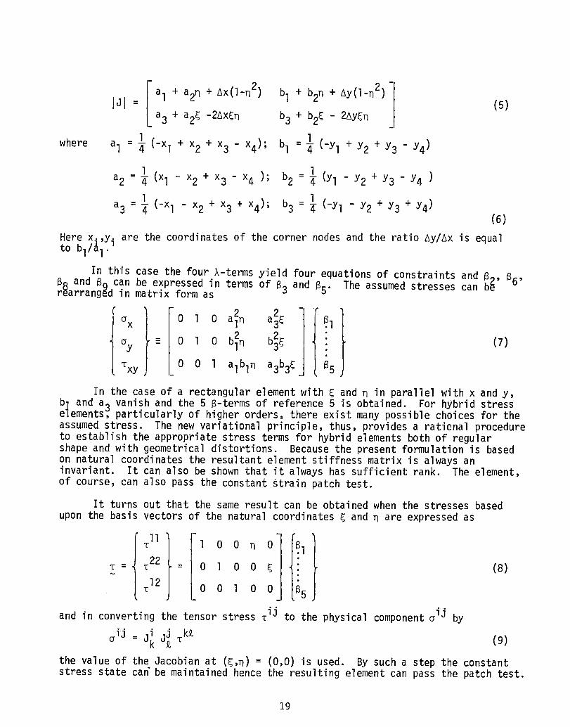
ij I a2n ) bI + b2n + Ay(l-n 2)= (5)a3 + a2_ -2Ax_n b3 + b2_ - 2Ay_n
where el = 1 (_Xl + x2 + x3- x4); bl : 1 (-Yl + Y2 + Y3- Y4)
a2 : 1 (x I _ x2 + x3 - x4 ); b2 : 1 (Yl - Y2 + Y3 - Y4 )
a3 = _ (-x I - x2 + x3 . x4); b_o = (-Yl - Y2 + Y3 + Y4)(6)
Here / I-x_'yi are the coordinates of the corner nodes and the ratio Ay/Ax is equalto bI
In this case the four _-terms yield four equations of constraints and R_, B6,B8 and BQ can be expressed in terms of B3 and B5. The assumed stresses canrearranged in matrix form as
IOX 0 1 0 a_n a_ _.I
_--oi oOy (7)
Txy 0 0 1 albln a3b3__ _5
In the case of a rectangular element with _ and n in parallel with x and y,b] and a3 vanish and the 5 B-terms of reference 5 is obtained. For hybrid stresselements, particularly of higher orders, there exist many possible choices for theassumed stress. The new variational principle, thus, provides a rational procedureto establish the appropriate stress terms for hybrid elements both of regularshape and with geometrical distortions. Because the present formulation is basedon natural coordinates the resultant element stiffness matrix is always aninvariant. It can also be shown that it always has sufficient rank. The element,of course, can also pass the constant strain patch test.
It turns out that the same result can be obtained when the stresses basedupon the basis vectors of the natural coordinates _ and n are expressed as
{ ilITII 1 0 0 n 0 ._I
T = T22 = 0 1 0 0 _ (8)
T12 0 0 l 0 0 5• • , °
and in convertingthe tensor stress Tlj to the physical componentoIj by
ij i " k_= Jk J_ T (g)
the value of the Jacobianat (_,n)= (0,0) is used. By such a step the constantstress state can"be maintainedhence the resultingelementcan pass the patch test.
19
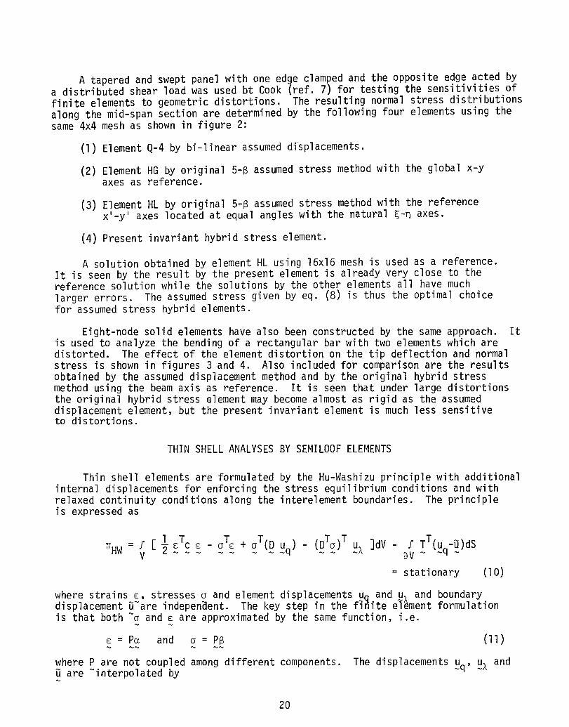
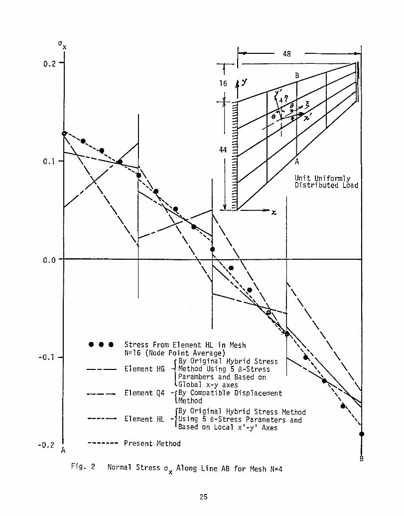
A tapered and swept panel with one edge clamped and the opposite edge acted bya distributed shear load was used bt Cook (ref. 7) for testing the sensitivities offinite elements to geometric distortions. The resulting normal stress distributionsalong the mid-span section are determined by the following four elements using thesame 4x4 mesh as shown in figure 2:
(I) Element Q-4 by bi-linear assumed displacements.
(2) Element HG by original 5-B assumed stress method with the global x-yaxes as reference.
(3) Element HL by original 5-8 assumed stress method with the referencex'-y' axes located at equal angles with the natural _-n axes.
(4) Present invariant hybrid stress element.
A solution obtained by element HL using 16x16 mesh is used as a reference.It is seen by the result by the present element is already very close to thereference solution while the solutions by the other elements all have muchlarger errors. The assumed stress given by eq. (8) is thus the optimal choicefor assumed stress hybrid elements.
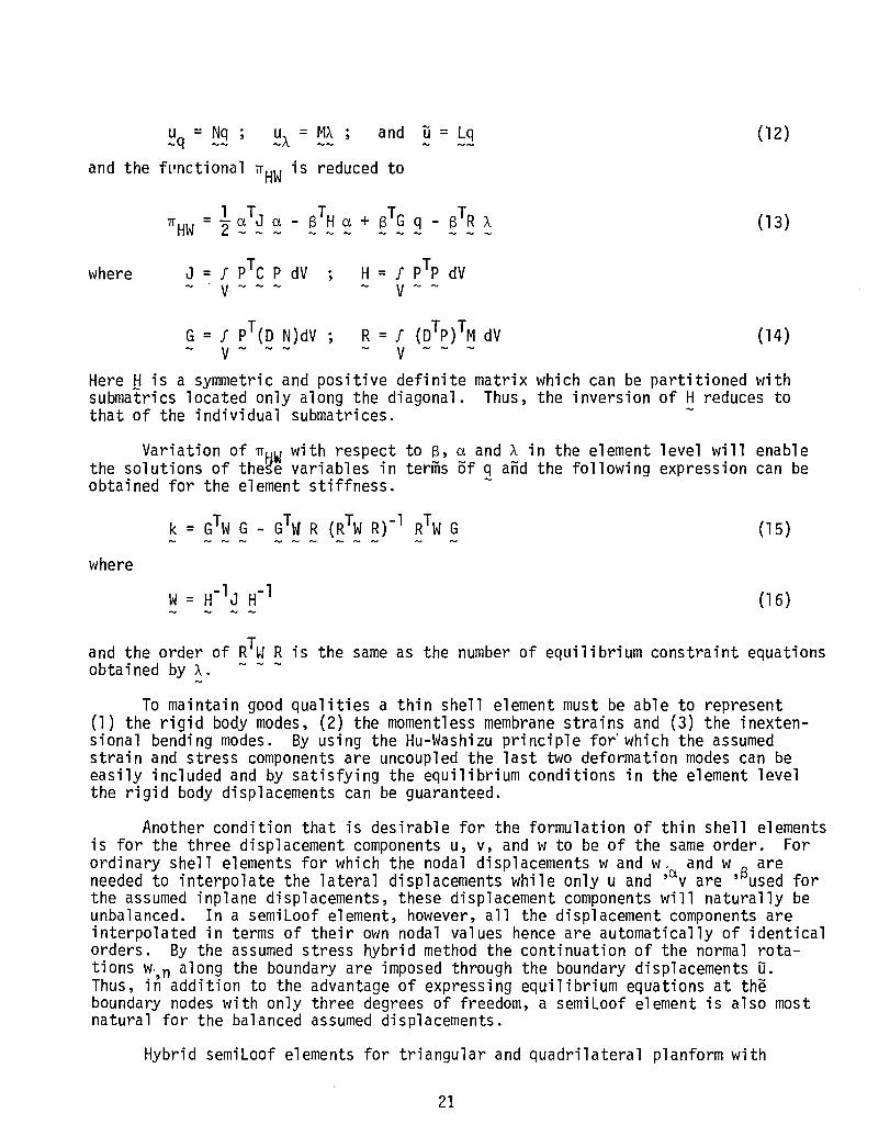
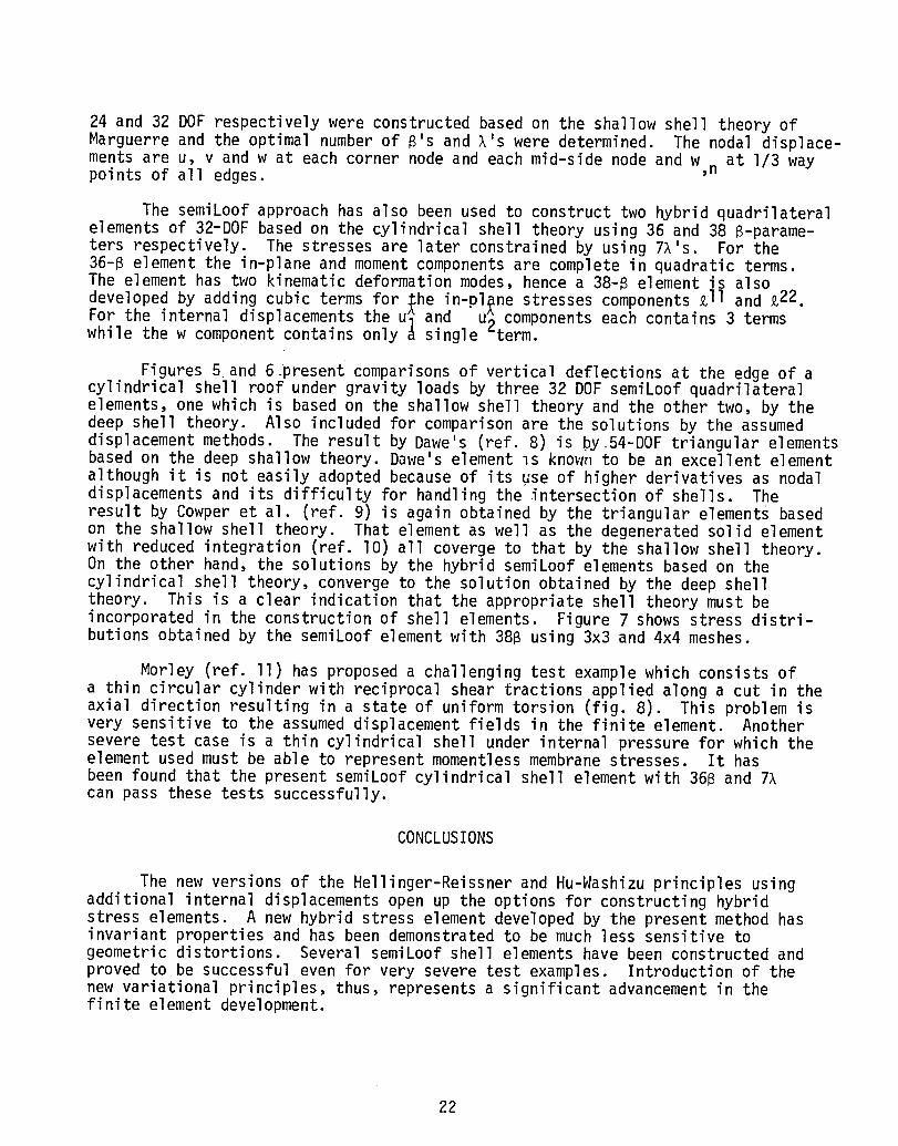
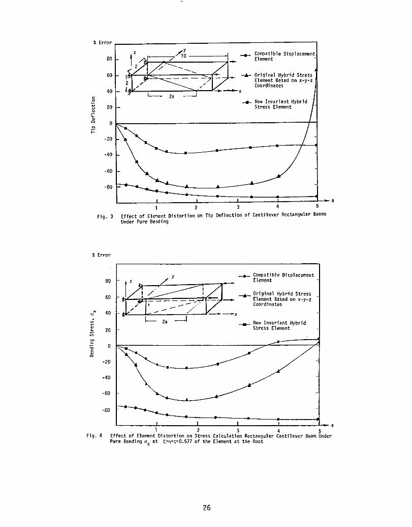
Eight-node solid elements have also been constructed by the same approach. Itis used to analyze the bending of a rectangular bar with two elements which aredistorted. The effect of the element distortion on the tip deflection and normalstress is shown in figures 3 and 4. Also included for comparison are the resultsobtained by the assumed displacement method and by the original hybrid stressmethod using the beamaxis as reference. It is seen that under large distortionsthe original hybrid stress element may become almost as rigid as the assumeddisplacement element, but the present invariant element is much less sensitiveto distortions.
THIN SHELLANALYSESBY SEMILOOFELEMENTS
Thin shell elements are formulated by the Hu-Washizu principle with additionalinternal displacements for enforcing the stress equilibrium conditions and withrelaxed continuity conditions along the interelement boundaries. The principleis expressed as
_HW= fv [ ½ ........._Tc e - T + oT(D Uq) _ (DT)T u_ ]dV - aVf TT~(_q-_)ds~
= stationary (I0)
where strains e, stresses o and element displacements uQ and u. and boundarydisplacement _~are indepenBent. The key step in the f_6ite el_ment formulationis that both ~o and e are approximated by the same function, i.e.
= P_ and o = PB (II)
where P are not coupled among different components. The displacements Uq, ux andare ~interpolated by
~
2O
Uq : Nq ; u_ = ~~M_; and ~_= ~~Lq (12)
and the functional _HWis reduced to
_ 1 Tj _ _ 8TH_ + 8TGq _ 8TR)_ (13)_HW- 2 ............
where J = Z pTc P dV ; H = Z pTp dV~ V .... V ~~
G = I pT(D N)dV ; R = f (DTp)TM dV (14)~ V ~ V
Here H is a symmetric and positive definite matrix which can be partitioned withsubmatrics located only along the diagonal. Thus, the inversion of H reduces tothat of the individual submatrices. ~
Variation of _HWwith respect to 8, _ and _ in the element level will enablethe solutions of the_ variables in terms _f q and the following expression can beobtained for the element stiffness. ~
k = GTwG - GTwR (RTw R)-I RTw G (15)
where
W = H-Ij H-I (16)
and the order of RTwR is the same as the number of equilibrium constraint equationsobtained by _. ~ ~ ~
~
To maintain good qualities a thin shell element must be able to represent(I) the rigid body modes, (2) the momentless membrane strains and (3) the inexten-sional bending modes. By using the Hu-Washizu principle for'which the assumedstrain and stress components are uncoupled the last two deformation modes can beeasily included and by satisfying the equilibrium conditions in the element levelthe rigid body displacements can be guaranteed.
Another condition that is desirable for the formulation of thin shell elementsis for the three displacement components u, v, and w to be of the same order. Forordinary shell elements for which the nodal displacements w and w. and w _ areneeded to interpolate the lateral displacements while only u and '_v are 'mused forthe assumed inplane displacements, these displacement components will naturally beunbalanced. In a semiLoof element, however, all the displacement components areinterpolated in terms of their own nodal values hence are automatically of identicalorders. By the assumed stress hybrid method the continuation of the normal rota-tions w n along the boundary are imposed through the boundary displacements _.Thus, i_ addition to the advantage of expressing equilibrium equations at th_boundary nodes with only three degrees of freedom, a semiLoof element is also mostnatural for the balanced assumed displacements.
Hybrid semiLoof elements for triangular and quadrilateral planform with
21
24 and 32 DOFrespectively were constructed based on the shallow shell theory ofMarguerre and the optimal number of B's and _'s were determined. The nodal displace-ments are u, v and w at each corner node and each mid-side node and w at I/3 waypoints of all edges. ,n
The semiLoof approach has also been used to construct two hybrid quadrilateralelements of 32-DOF based on the cylindrical shell theory using 36 and 38 B-parame-ters respectively. The stresses are later constrained by using 7_'s. For the36-B element the in-plane and moment components are complete in quadratic terms.The element has two kinematic deformation modes, hence a 38-B element is alsodeveloped by adding cubic terms for _he in-ol_ne stresses components £II and £22For the internal displacements the u_ and 'u_ components each contains 3 terms
o
while the w component contains only _ single :term.
Figures 5 and 6 present comparisons of vertical deflections at the edge of acylindrical shell roof under gravity loads by three 32 DOFsemiLoof quadrilateralelements, one which is based on the shallow shell theory and the other two, by thedeep shell theory. Also included for comparison are the solutions by the assumeddisplacement methods. The result by Dawe's (ref. 8) is by_54-DOF triangular elementsbased on the deep shallow theory. Dawe's element Is known to be an excellent elementalthough it is not easily adopted because of its _se of higher derivatives as nodaldisplacements and its difficulty for handling the intersection of shells. Theresult by Cowper et al. (ref. 9) is again obtained by the triangular elements basedon the shallow shell theory. That element as well as the degenerated solid elementwith reduced integration (ref. I0) all coverge to that by the shallow shell theory.On the other hand, the solutions by the hybrid semiLoof elements based on thecylindrical shell theory, converge to the solution obtained by the deep shelltheory. This is a clear indication that the appropriate shell theory must beincorporated in the construction of shell elements. Figure 7 shows stress distri-butions obtained by the semiLoof element with 38B using 3x3 and 4x4 meshes.
Morley (ref. II) has proposed a challenging test example which consists ofa thin circular cylinder with reciprocal shear tractions applied along a cut in theaxial direction resulting in a state of uniform torsion (fig. 8). This problem isvery sensitive to the assumed displacement fields in the finite element. Anothersevere test case is a thin cylindrical shell under internal pressure for which theelement used must be able to represent momentless membrane stresses. It hasbeen found that the present semiLoof cylindrical shell element with 36B and 7_can pass these tests successfully.
CONCLUSIONS
The new versions of the Hellinger-Reissner and Hu-Washizu principles usingadditional internal displacements open up the options for constructing hybridstress elements. A new hybrid stress element developed by the present method hasinvariant properties and has been demonstrated to be much less sensitive togeometric distortions. Several semiLoof shell elements have been constructed andproved to be successful even for very severe test examples. Introduction of thenew variational principles, thus, represents a significant advancement in thefinite element development.
22
REFERENCES
I. Pian, T.H.H; and Tong, P.: Basis of Finite Element Methods for Solid Continua.Int. J. Num. Meth. Engng, vol. I, 1968, pp. 3-28.
2. Pian, T.H.H.: Finite Element Methods by Variational Principles with RelaxedContinuity Requirements. Variational Methods in Engineering, C.A. Brebbiaand H. Tottenham (Ed.), Southampton Univ. Press, 1973, pp. 3/I-3/24.
3. Pian, T.H.H.; and Chen, D.P.: Alternative Ways for Formulation of HybridStress Elements. Int. J. Num. Meth. Engng., vol. 18, 1982, pp. 1679-1684.
4. Pian, T.H.H.; Chen, D.P.; and Kang, D.: A New Formulation of Hybrid/MixedFinite Elements. Computers and Structures, vol. 16, 1983, pp. 81-87.
5. Pian, T.H.H.: Derivation of Element Stiffness Matrices by Assumed StressDistributions. AIAA J., vol. 2, 1964, pp. 1333-1336.
6. Wilson, E.L.; Taylor, R.L.; Doherty, W.; and Ghaboussi, J.: ImcompatibleDisplacement Models. Numerical and Computer Methods in Structural Mechanics,(Eds. S.J. Fenves et al.), Academic Press, 1973, pp. 43-57.
7. Cook, R.D.: Improved Two-Dimensional Finite Element. ASCEJ. Structural Div.,ST9, Sept. 1974, pp. 1851-1863.
8. Dawe, D.J.: High-Order Triangular Finite Element for Shell Analysis. Int.J. Solids Structures, vol. II, 1975, pp. 1097-1110.
9. Cowper, G.R.; Lindberg, G.M.; and Olson, M.D.: A Shallow Shell Finite ElementTriangular Shape. Int. J. Solids Structures, vol. 6, 1970, pp. 1133-1156.
I0. Zienkiewicz, O.C.; Taylor, R.L.; and Too, T.M.: Reduced Integration Techniquein General Analysis of Plates and Shells. Int. J. Num. Meth. Engng., vol. 3,1971, pp. 275-290.
II. Morley, L.S.D.: Analysis of Developable Shells with Special Reference to theFinite Element Method and Circular Cylinders. Phil. Trans. Roy. Soc.London, vol. 281, no. 1300, 1976, pp. 113-170.
23
(x3,Y 3)
(x4,Y 4
(x2,Y 2)
\Yl (Xl'Yl)
X
(x3,Y 3)x2+x3 Y2+Y3
3 (_ + &x' 2 + Zly)
4
(x4'Y4) __Z_y&x
(x2,Y 2)Ay 2
xl+x 4 YI+Y4( 2 AX' 2 Ay)
Y I (Xl 'Yl )-"- x
Fig. 1 Quadrilateral Element with Small Perturbation
24
/
\ "e.___-.,./ 44
o.i- \-'-_
Unit Uniformly_ Distributed Load
/ \\
_I" \ . \\ , \
0.0 \ •i
\ • \
\ \ \\
\\
• • • Stress From Element HL in Mesh \
-0.I - N=I6 (Node Point Average) _ \f By Original Hybrid Stress
Element HG -_Method Using 5 B-Stress "- \
|Parambers and Based on _ \\kGlobal x-y axesN__ Element Q4 -_By Compatible Displacement \_ _
LMethod
_By Original Hybrid Stress Method \Element HL -IUsing 5 B-Stress Parameters and _
_Based on Local x'-y' Axes
-0.2 Present MethodA
B
Fig. 2 Normal Stress ox Along Line AB for Mesh N=4
25
% Error
A z , _I_ _ CompatibleDisplacement80 l _I" • / I Element
60 Original Hybrid Stress
fl Coordinates40 i;r I-_ 2a ------J
_ New InvariantHybrid I
20 - Stress Ele_nt /
o
-20
-40
-6O
-80
I ! I I _al 2 3 4 5
Fig. 3 Effect of El_ent Distortionon Tip Deflectionof CantileverRectangularBeamsUnder Pure Bending
% Error
y _ CompatibleDisplacement
80 z ./ _ _ Element
60 _[___/_ +Origlnal Hybrid StressElement Based on x-y-z
x 40 I / /_"'" X
_ 2a _ New InvariantHybridStress Element
20
-20
-40
-60
-80
I I t _ aI 2 3 4 s
Fig.4 Effectof ElementDistortionon StressCalculationRectangularCantileverBeamUnderPureBendingox at _=n=_=0.577of the Elementat theRoot
26

32 DOFSEMILOOFELEMENT
O-- U,V,W59Bs4 _--w
,nExact (Shallow Shell )
: 3 70331
€-O
" / .. Cowper,Lindbergand
/ Olson
/ 0--------QuadrilateralElement- (Shallow Shell Theory)
" it_Q,I
!
2- [
I I I I I0 lO0 200 300 400 500 (DOF)
Fig. 5 Convergence of Vertical Deflection at D for Cylindrical ShellRoof Problem
27
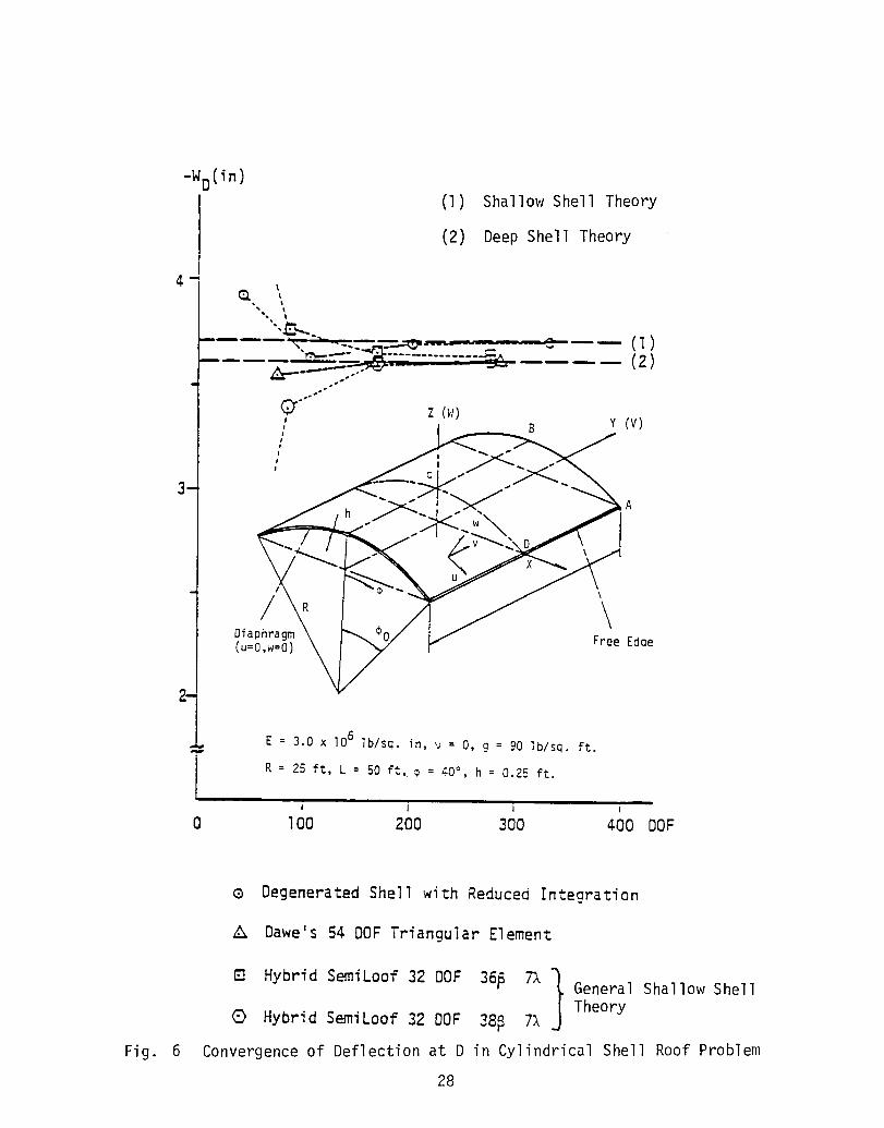
-WD(in)(I) Shallow Shell Theory
(2) Deep Shell Theory
-- \
\Diaphragm FreeEdae(u:O,w:O)
E : 3.0 x 10⁶ Ib/sq. in, v = O, g = 90 Ib/sq. ft.
T R : 25 ft, L = 50 ft, _ : 40°, h : 0.25 ft.i i i i
0 I00 200 300 400 DOF
C) DegeneratedShell with Reduced In:egra:ion
AS Dawe's 54 DOF Triangular Element
[] Hybrid SemiLoof 32 DOF 36/_ TX I GeneralShallowShell
]TheoryHybrid SemiLoof 32 DOF 38_ 7_
Fig. 6 Convergenceof Deflectionat D in CylindricalShell Roof Problem
28

2
Ny _P M_
(ki p/f t) (ft. Ki p/f t)
at y=O -40 - • at y=O1
oI O _ 5
40 Ny
80 I I I
0 10 20 30 40(o)
0 Hybrid SemiLoof 38B 7_ 4x4 Mesh
(_ Hybrid SemiLoof 38_ 7_ 3x3 Mesh
Fig. 7 Stress Distribution in Cylindrical Shell Roof Problem
LC
B
Rec_proca| Shear
Fig. 8 Shear Load on a Slit Cylinder
29


A SHEAR DEFORMABLE SHELL ELEMENT
FOR LAMINATED COMPOSITES i
W. C. Chao and J. N. Reddy
Department of Engineering Science and Mechanics
Virginia Polytechnic Institute and State University
Blacksburg, VA 24061
SUMMARY
A three-dimensional element based on the total lagrangian description of the
motion of a layered anisotropic composite medium is developed, validated, and used
to analyze layered composite shells. The element contains the following features:
geometric nonlinearity, dynamic (transient) behavior, and arbitrary lamination
scheme and lamina properties. Numerical results of nonlinear bending, natural
vibration, and transient response are presented to illustrate the capabilities ofthe element.
INTRODUCTION
Composite materials and reinforced plastics are increasingly used in
automobiles, aircrafts, space vehicles, and pressure vessels. With the increased use
of fiber-reinforced composites as structural elements, studies involving the
thermomechanical behavior of shell components made of composites are receiving
considerable attention. Functional requirements and economic considerations of
design have forced designers to use accurate but economical methods of determining
stresses, natural frequencies, buckling loads, etc. The majority of the research
papers in the open literature on shells is concerned with bending, vibration, and
buckling of isotropic shells. As composite materials are making their way into manyengineering structures, analyses of shells made of such materials become
important. The application of advanced fiber composites in jet engine fan or
compressor blades and high performance aircraft require studies involving transient
response of composite shell structures to assess the capability of these materialsunder dynamic loads.
A review of the literature indicates that first, there does not exist any
finite-element analysis of geometrically nonlinear transient response of laminatedanisotropic shells, and second, the 3-D degenerated element is not exploited for
geometrically nonlinear analysis of laminated anisotropic shells. The present study
was undertaken to develop a finite-element analysis capability for the static and
dynamic analysis of geometrically nonlinear theory of layered anisotropic shells. A
tA more detailed account of this paper can be found in NASA CR-168182.
31

3-D degenerated element with total Lagrangian description is developed and used to
analyze various shell problems.
INCREMENTAL, TOTAL-LAGRANGIAN FOR!_LATION OF A CONTINUOUS MEDIUM
The primary objective of this section is to review the formulation of equations
governing geometrically nonlinear motion of a continuous medium. In the interest of
brevity only necessary equations are presented (see [i-5]).
We describe the motion of a continuous body in a Cartesian coordinate system.
The simultaneous position of all material points (i.e., the configuration) of the
body at time t is denoted by Ct, and Co and Ct+6t denote the configurations at
reference time t = 0 and time t + 6t, respectively. In the total Lagrangian
description all dependent variables are referred to the reference configuration.
The coordinates of a typical point in Ct is denoted by tx = (txl,tx2,tx3). The
displacement of a particle at time t is given by
t t o t t ou~= ~x- ~x or u.z = xi - xi (i)
The increment of displacement during time t to t + 6t is defined by
t+6t t
ui -- ui - ui (2)
The principle of virtual displacements can be employed to write the equilibrium
equations at any fixed time t. Xhe principle, applied to the large-displacements
case, can be expressed mathematically as
t+6t'" t+6t S. (t+6t )dVf Po u. 6u. dV + f lj 6 Eij oV z z o V
o o
= f t+6tT. 6ui dA + f t+6tF. 6u. dV (3)1 O 1 1 OA Vo o
where summation on repeated indices is implied; Vo, Ao, and Po denote, respectively,
a volume element, area element, and density in the initial configuration, Sij are
the components of second the Piola-Kirchhoff stress tensor, gij the components of
the Green-LaKrangianstran tensor,Ti the componentsof boundary stresses,and Fi
are the componentsof the body force vector. _he superposeddots on ui denote
differentiationwith respectto time, and 6 denotes the variationalsymbol. In
thewritingkinematicEq"(3)relationsit is assumed that Eij is related to the displacement components by
t+6t 1 (t+6tui + t+6t t+6t t+6tEij=y ,j u.. + u u .) (4)3,z m,i m,3
where ui,j = 5ui/Sxj.
32

t+6tThe stress components S.. can be decomposed into two parts:
13
t+6t S t S.ij = lj + Sij (5)
where Sij is the incremental stress tensor. The incremental stress components Sij
are related to the incremental Green-L_grange strain components, Eij = eij + qi j, bythe generalized Hooke's law:
Sij = Cijk%gk%, (6)
where Cijk% are the components of the elasticity tensor. Using Eqs. (4)-(6), one
can be express Eq. (3) in the alternate form
f Po t+6t ""u.6u. dV + f Cijki(eki6_j + _ki6eij )dVV I 1 o V oo o
+ f tsij 6eij dVo = 6W- f ts'i 6_i j dVo (7)V V 1o o
where _ is the virtual work due to external loads.
FINIT_ELEMENT MODEL
The coordinates of a typical point in the element can be written as (see
Fig. i)
n n
= Z _(_i,_2)_____ (x )top + Z +j(_1,_2 ) i_ jxi j=l j=l -- (Xi)bottom (8)
where n is the number of nodes, li(_l,_2 ) are the finite-element interpolation (or
shape) functions, which, in the element take the value of unity at node i and zero
at all other nodes, _i and _2 are the normalized curvilinear coordinates in the
middle plane of the shell, and g is a linear coordinate in the thickness directioni i i
and Xl, x2, and x3 are the global coordinates at node i.
tIn the present study the current coordinates x. are interpolated by the
expression i
t n j 1 t^jx = Z qbj(tx + (9)i j=l _ Chj e 3iO_
and the displacements by
nt ° ^ ° ^ "
u = E +j [tuJ'l+ I (t J _ o Ji _ _hj e3i e3i) ] (i0)j=l
^ •
n I t+AteJ teO ) ] (ii)u = Z + [uj +- _h (i j i 2 j 3i 3i
j=l
33

o 3-D Element
n 2-D Element
/x Reference[6]3.0 --
R/a = 10, a/b = 1 /
_2.5_ a/h = 80 //
02.0
o
o_ 1 _ 1.5
JT °x3' _3 >
/_1.0
4_ ..... --_ xl'_I a - 254m, b - 254m,R " 2540 ram.h - 3.175 ram,
e " 0.1 rad.
Figure i. Geometry of the degenerated 0.5 an fouredgesareclamped:U'V_W_x'_ysOthree-dimensional element
O. , I t I I I , I , I I IO. 2. 4. 6. 8. lO. 12.
Centerdeflecti0n,w (inmm)
Figure 2. Load-deflection curve for a clampedcylindrical shell under uniform load

tu_ and ul denote, respectively, the displacement and incremental displacementHere
components in the xi-direction at the j-th node.
Substitution of Eqs. (4)-(6) and (9)-(11) into Eq. (7) yields
f Po[T]t{u}dVo + (t[KL] + t[KNL]){A } = t+6t{R} - t+6t{F} (12)Vo
where t[KL] , t[KNL], {R}, and {F} are the linear and nonlinear stiffness matrices,
force vector, and unbalanced force vectors
Application of the New,hark direct integration scheme (see [2]) for theapproximation of the time derivatives in Eq. (12) leads to
[K]{A} = t+6tlR I - t+6t{F}(k-l) (13)
where
[K] = a t[M] + t[K]O
^ _i (t{ t{t+6t{R} = t+6t{R} + a2 [t{Pl} _ P2} - P3})] + a3 {P4} (i4)
and ao, a2, etc. are the parameters in the Newmark integration scheme.
DISCUSSION OF THE N[_ERICAL RESULTS
The results to be discussed are grouped into three major categories:
(1) static bending, (2) natural vibration, and (3) transient response. All results,
except for the vibrations, are presented in a graphical form. All of the results
presented here were obtained on an IBM 370/3081 computer with double precisionarithmatic.
Static Analysis
i. Cylindrical Shell Subjected to Radial Pressure Consider a circular
cylindrical panel, clamped along all four edges and subjected to uniform radial
inward pressure. The geometric and material properties are
R = 2540 am, a = b = 254 am, h = 3.175 am,
0 = 0.I rad, E = 3.10275 kN/mm 2, v = 0.3
Due to the symmetry of the geometry and deformation, only one quarter of the panel
is analyzed. A load step of 0.5 KN/m 2 was used in order to get a close
representation of the deformation path. Figure 2 shows the central deflection
versus the pressure for the panel dimensions a = 254 mm and b = 254 mm. The
solution for agrees very closely with that obtained by Dhatt [6] and the shell
element of Peddy [7].
35

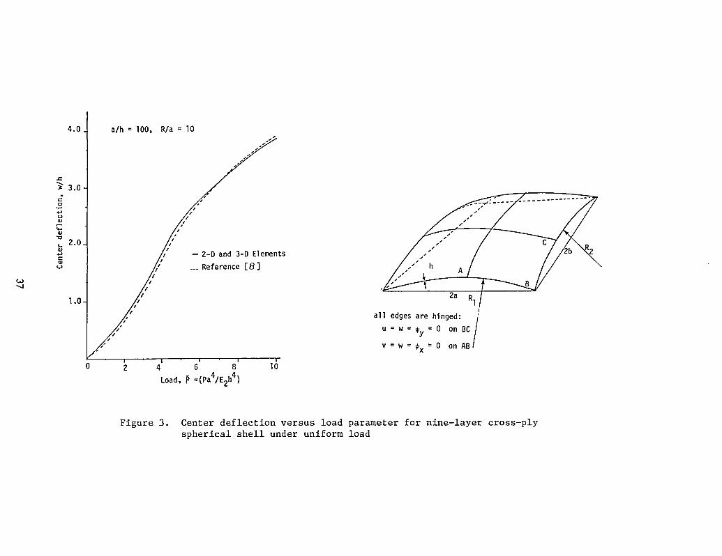
2. Nine-Layer Cross-Ply (0°/90°/0°/...) Spherical Shell Subjected to Uniform
Loading Consider a spherical shell laminated of nine layers of graphite-epoxy
material (EI/E 2 = 40, GI2/E 2 = 0.6, G13 = GI2 = G23 , v12 = 0.3), subjected to
uniformly distributed loading, and simply supported on all its edges (i.e. ,
transverse deflection and tangential rotations are zero). A comparison of the load-
deflection curves obtained by the present element with those obtained by Noor [8] is
presented (for the parameters h/a = 0.01 and R/a = i0) in Fig. 3. The results agree
very well with each other, the present 2-D results being closer to Noor's
solution. This is expected because Noor's element is based on a shell theory.
3. Two-Layer Cross-Ply and Angle-Ply (45°/-45 °) Shells Under Uniform LoadingThe geometry of the cylindrical shell used here is the same as that considered in
Problem I. The shell is assumed to be simply supported on all edges. The material
properties of individual lamina are the same as those used in Problem 2. A mesh of
2x2 nine-node elements in a quarter shell is used to model the problem. The results
of the analysis are presented in the form of load-deflection curves in Fig. 4. From
the results, one can conclude that the angle-ply shell is more stiffer than the
cross-ply shell. The geometry and boundary conditions used for the spherical shells
are the same as those used in Problem 2. The geometric parameters used are: R/a =
i0, a/h = i00. The load-deflection curves for the cross-ply and angle-ply shells
are shown in Fig. 5. From the plots it is apparent that, for the load range
considered, the angle-ply shell, being stiffer, does not exhibit much geometric
nonlinearity. The load-deflection curve of the cross-ply shell exhibits varyingdegree of nonlinearity with the load. For load values between i00 and 150, the
shell becomes relatively more flexible.
Natural Vibration of Twisted Plates
4. Natural vibration of cantilevered twisted plates Here we discuss the
results obtained for natural frequencies of various twisted plates. This analysiswas motivated by their relevance to natural vibrations of turbine blades. Consider
an isotropic cylindrical panel with a twist angle 6 at the free end. Table 1
contains the natural frequencies of a square plate for various values of the twistangle e and ratios of side to thickness. A 2x2 mesh and 4x4 mesh of 9-node elements
are employed to study the convergence trend. The results of the refined mesh are
included in the parentheses. The results agree with many others published in a
recent NASA report.
Transient Analysis
5. Spherical Cap Under Axisymmetric Pressure Loading Consider a spherical
cap, clamped on the boundary and subjected to axisymmetric pressure loading, Po"The geometric and material properties are
R = 22.27 in., h = 0.41 in., E = 10.5 x 10⁶ psi, v --0.3,
p = 0.095 ib/in 3, 6 = 26.67 °, Po = i00 ksi, 6t = 10-5 sec.
This problem has been analyzed by Stricklin, et al. [9] using an axis_nmetric shell
element. In the present study the spherical cap is discretized into five nine-node
2-D or 3-D elements. Figure 6 shows the deflection of the center as a function of
time. The present solutions are in excellent agreement in most places with that of
36
4.0 a/h = 100, R/a = 10
3.0 ¢" , _ _ • "u
L 2.0_ ts
o ' ... Reference [8 ] A
",,,I('_ //j
!
all edges are hinged:
u = w : _y : 0 on BC
v = w = _x = 0 on ABI | i2 4 6 8 I0
Load, _ =(pa4/E2 h4)
Figure 3. Center deflection versus load parameter for nine-layer cross-ply
spherical shell under uniform load

2.5 R/a = I, a/h = 100 .oIi
,S_ o AP CPr- ID _
_ 0.24,3.0 AP = Angle-ply,£P = Cross-ply
-.f= "i5o 2.0 uu .-_0.20,2.5 o 2-D and 3-D Elements [O°/90°]
o 3-D Element
L1.5 _ 0.16,2.0= R/a = I0, a/h = I00
u(-O "I_ .N
o 2-D E ._ 0.12,1.5 45°/-45°]
_ 1.0 f / a 3-0 ElementT_
/ • 3-O Element,[45°/-45°] _ 0.08,1.0
/0.5
0.04,.:5 J/,/
0.0 0.0| i l , i _ . i , T
l _ i i !0 50 100 150 200 2S0 30 350 400 450 0 20 40 60 80 100 120 140 160 180 200 220 240
Loadparameter,P = (Pa4/E2h4) Loadparameter,P=(pa4/E2h4)
Figure 4. Center deflection versus load parameter Figure 5. Center deflection versus load para-
for two-layer composite cylindrical shell meter for composite spherical shell
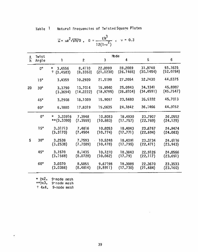
Table 1 NaturalFrequenciesof TwistedSquare Plates
_= _a2#'6h-7D, D - Eh3 , u = 0.3212(l-v )
a Twist Mode-h Angle l 2 3 4 5 6
0° * 3.4556 8.4110 22.0999 28.2089 31.9740 55.1625(3.4583) (8.3353) (21.0238) (26.7465) (30.I454) (52.0784)
15° 3.4359 10.2920 21.5199 27.2054 32.7430 44.5375
20 30° 3.3790 13.7014 19.9840 25.0943 34.3341 45.8987(3.3694) (14.2222)(18.9795) (26.8104) (34.4591) (45.7547)
45° 3.2908 18.1009 15.9097 23.5680 35.5332 45.7013
60° 6.1800 17.8319 15.5635 24.1842 36.1466 44.9152
0° * 3.33916 7.3948 I0.8083 18.4930 23.7907 26.0552•*(3.3390) (7.3559) (10.883) (17.757) (22.769) (24.125)
15° 3.31713 7.4816 10.8053 18.4043 23.6767 24.9474(3.3170) (7.4504 (I0.774) (17.771) (22.694) (24.083)
5 30° 3.2538 7.7593 10.5248 18.4091 23.3734 24.6116(3.2538) (7.7089) (I0.478) (17.795) (22.471) (23.943)
45° 3.1570 8.1435 I0.1270 18.3843 22.9126 24.0566(3.!569) (8.0728) (10.062) (17.79) (22.117) (23.651)
60° 3.0370 8.5855 9.67198 18.3089 22.3670 23.3533(3.0366) (8.4814) (8.5911) (17.730) (21.684) (23.160)
* 2x2, 9-node mesh*-3x3, 9-node mesht 4x4, 9-nodemesh
39

Stricklin et al [9]. The difference between the solutions is mostly in the regionsof local minimum and maximum.
6. Two-Layer Cross-Ply Cylindrical Shell Under Uniform Load A cylindrical
shell with a = b = 5", R = i0", h = 0.i" is simply-supported on the four edges. The
deep shell is laminated by 2 layers (0°/90 °) and exerted by a uniform step load
^ (a4p/E2h4P = ) Figure 7 contains a plot of the center deflection versus time for 2-
D and 3-D elements. The time step used is 6t = 0.i x 10-4 sec. The solutions
obtained 2-D shell element and 3-D degenerate element are in good agreement.
7. Four-layer Angle Ply (45°/-45°/45°/-45 °) Cylindrical Shell Under Uniform
Load Here we present result for a cylindrical shell which has the same geometry as^
in Problem 3 above. The shell is subjected to a uniform step load P = 50. Figure4.8 contains a plot of the center deflection versus time for 2-D and 3-D elements.
The two elements yield solutions that agree very well in the beginning of the cycle,and the 2-D element gives negative values of the deflection at the end of the
cycle. The discrepency is due to the fact that the 2-D element does not account for
geometric changes from one time step to next.
8. Two-layer Angle-Ply (45°/-45 °) Spherical S_ell Under Uniform loading
Consider a spherical shell with a = b = i0", R = 20" and h = 0.i", simply supported
at four edges and is exerted by a uniform step load. The shell consists o_ twolayers, (45°/-45°). Figure 9 shows the center deflection versus time for P = 50
^
and P = 500 with time step 0.2 x 10⁻⁵ sec. For the small load the curve is
relatively smooth compared to that of the larger load. This is due to the fact that^ A
the geometric nonlinearity exhibited at P = 50 is smaller compared to that at P =500.
The results of Problems 3, 4, 6, 7, and 8 should serve as references for future
investigations. For additional results the reader is referred to Reference i0.This completes the discussion of the results.
CONCLUSIONS
The present 3-D degenerated element has computational simplicity over a fullythree-dimensional element and the element accounts for full geometric nonlinearitiesin contrast to 2-D elements based on shell theories. As demonstrated via numerical
examples, the deflections obtained by the 2-D shell element deviate from those
obtained by the 3-D element for deep shells. Further, the 3-D element can be used
to model general shells that are not necessarily doubly-curved. For example, thevibration of twisted plates cannot be studied using the 2-D shell element discussed
in [7]. Of course, the 3-D degenerated element is computationally more demanding
than the 2-D shell theory element for a given problem. In summary, the present 3-Delement is an efficient element for the analysis of layered composite plates and
shells undergoing large displacements and transient motion.
The 3-D element presented herein can be modified to include thermal stress
analysis capability and material nonlinearities. While the inclusion of thermal
stresses is a simple exercise, the inclusion of nonlinear material effects is a
difficult task. An acceptable material model should be a generalization of Ramberg-
Osgood relation to a layered anisotropic medium. Another area that requires further
4O

Figure 6. Center deflection versus time for a Figure 7. Center deflection versus time for a
spherical cap under axisymmetric dynamic two-layer cross-ply cylindrical shell
load (Po = i00 psi) under uniform step load

Figure 8. Center deflection versus time for four- Figure 9. Center deflection versus time for two-
layer angle-ply [450/-450/45°/-45 °] layer angle-ply [45°/-45 °] sphericalcylindrical shell under uniform load shell under uniform load
study is the inclusion of damping effects, which are more significant than the sheardeformation effects.
Acknowledgments
The present study was conducted under a research grant from the Structures
Research Section of NASA lewis Research Center. _he authors are very grateful for
the support and encouragement by Dr. C. C. Chamls of NASA/Lewis. It is also a
pleasure to acknowledge the typing of the manuscript by Mrs. Vanessa McCoy.
REFERENCES
i. B. Krakeland, "Nonlinear Analysis of Shells Using Degenerate Isoparametrlc
Elements ," Finite Elements in Nonlinear Mechanics, International Cbnference on
Finite Elements in Nonlinear Solid and Structural Mechanics, At Geilo, Norway,Aug. 1977, pp. 265-284.
2. K. J. Bathe, E. Ramm and E. L. Wilson, "Finite Element Formulations for Large
Deformation Dynamic _alysis," International Journal for Numerical Methods inEngineering, Vol. 9, 1975, pp. 353-386.
3. G.A. Dupuris, H. D. Hibblt, S. F. McNamara and P. V. Marcal, "Nonlinear
Material and Geometric Behavior of Shell Structures," Computers and Structures,
Vol. i, 1971, pp. 223-239.
4. G. Horrigmoe and P. G. Bergan, "Nonlinear Analysis of Free-Form Shells by Flat
Finite Elements,'° Computer Methods in Applied Mechanics and _gineering, 16,
1978, pp. 11-35.
5. S. Ahmad, B. M. Irons and O. C. Zienkiewicz, °'Analysis of Thick and Thin Shell
Structures by Curved Finite Elements," International Journal for Numerical
Methods in Engineering, 2, 1970, pp. 419-451.
6. G. S. _att, "Instability of _hin _ells by the Finite Element Method," 1ASS
Symposium for Folded Plates and Prismatic Structures, Vienna, 1970.
7. J. N. Peddy, °'Bending of Laminated _nisotropic _hells by a _ear Deformable
Finite Element," Fibre Science and Technology, Vol. 17, pp. 9-24, 1982.
8. A. K. Noor and S. J. Pmrtley, '°Nonlinear _hell _nalysis Via Mixed Isoparametric
Elements," Computers and Structures, Vol. 7, 1977, pp. 615-626.
9. J.A. Stricklin, J. E. Martinez, J. R. Xlllerson, J. H. Nong, and W. E.
Haisler, "Nonlinear Dynamic Analysis of Shells of Revolution by Matrix
_isplacement Method," AIAA, Vol. 9, No. 4, April 1974, pp. 629-636.
i0. W. C. Chao and J. N. Reddy, °'Geometrically Nonlinear Analysis of Layered
Composite Plates and Shells," NACA CR-168182, Virginia Polytechnic Institute,,
Blacksburg, VA 24061, 1983.
43


NONLINEARFINITE ELEMENTANALYSISOF SHELLSWITH
LARGEASPECTRATIO*
T. Y. Changand K. SawamiphakdiThe University of Akron
SUMMARY
A higher order 'degenerated' shell element with 9-nodes was selected for largedeformation and post-buckling analysis of thick or thin shells. Elastic-plastic ma-terial properties may also be included. A description on the post-buckling analysisalgorithm is given. Using a square plate, it was demonstrated that the 9-node ele-ment does not have shear locking effect even if its aspect ratio was increased tothe order 108 Two sample problems are given to show the analysis capability of theshell element.
INTRODUCTION
Research work in finite element analysis applied to plates and shells has en-dured for more than twenty years due to the complexity of the problems involved.Continuing progress is still being made on topics relating to nonlinear shell analy-sis. In particular, recent interest has been focused on large deformation and post-buckling behavior of shells. Applications of such analysis problems can be foundin turbine blades, nuclear vessels and offshore tubular members, etc.
Development of a finite element procedure for plate or shell analysis can beachieved by two distinct approaches: i) using classical shell theories or ii) de-riving finite element equations directly from the three dimensional continuum theory.Although there are several shell theories of different approximations [1] which areuseful for linear analysis, they cannot be readily extended to nonlinear cases withsufficient generality. Consequently, most of the recent nonlinear shell researchwas concentrated in the latter approach.
Based on the three-dimensional continuum theory, several different directionscan be pursued to formulate a shell element. One approach is to deduce a shell ele-ment from a 3/D isoparametric solid by imposing necessary kinematic assumptions inconnection with the small dimension of the shell thickness. Adoption of isoparame-tric formulation offers two immediate advantages: i) the requirement of rigid bodymodes is satisfied, and ii) element properties are invariant with reference coordi-nates. Several variations of isoparametric-base shell elements have appeared in theliterature. One class of elements is the so-called 'degenerated' shell family with4 to 16 nodes, which was originally proposed by Ahmad, Iron and Zienkiewicz [2] forlinear shells. Although these elements are quite versatile for extension to nonline-ar analysis, several numerical difficulties were experienced. The most notoriousproblem is that the lower order elements exhibit shear-locking phenomenon as thethickness of the shell becomessmall (or large aspect ratio-element size vs. thick-ness). One way to circumvent this problem is to adopt a reduced integration tech-
*Work supported by NASAGrant NASG3-317.
45
nique for evaluation of element stiffness. An alternate solution is to use higherorder elements, such as 9- or 16-node Lagrange element.
In this paper, some of the recent nonlinear analysis results for a 9-node 'de-generated' shell element are reported. Nonlinearities considered in our work includelarge deformations, post-buckling behavior and elastic-plastic materials.
DEGENERATEDSHELLELEMENT
Detailed description of this element can be found in [3,4] and therefore willnot be repeated herein. Wewill only briefly outline this element for the sake ofcompleteness. The geometry of the element is circumscribed by its middle surfacewhich consists of 9-nodes as shown in Fig. I. Each node has five degrees of free-dom, three translations in the direction of global axes and two rotations about alocal system. Displacement patterns in the surface of the shell are represented byquadratic polynomials. Whereas in the thickness direction, displacements are approx-imated by Mindlin's plate assumptions. If the center node of the element is removed,it reduces to an 8-node serendipity element. Otherwise, the element is called a 9-node Lagrange element.
SOLUTIONMETHOD
The nonlinear shell equations are solved by an incremental tangent stiffnessapproach. For each load increment, either the full or modified Newton-Raphson algo-rithm can be optioned in conjunction with secant accelerated iterations. For shellsexhibiting softening behavior, the modified Newton-Raphson with or without acceler-ated iterations was found most effective. On the other hand, for shells exhibitingstiffening effect or near instability, the full Newton-Raphson algorithm is necessaryfor obtaining convergent solutions. However, if one is to follow the structural re-sponse of a shell beyond its instability point (post-buckling behavior), any of theaforementioned algorithms fails to apply due to the singularity of tangent stiffnessmatrix. For this purpose, a different algorithm must be employed.
There are at least four different methods available for post-buckling analysis:i) Artificial spring, ii) specified displacements at nodes, iii) use of currentstiffness, and iv) constrained arc length. A comprehensive review of these methodswas given by Ramm[5] and Riks [6]. Of all the methods that have been applied topost-buckling analysis of shells, the constrained arc length is most effective dueto its generality. Actually, in concept this method is equivalent to a displacementcontrol analysis, in which numerical instability of a system is circumvented byspecified boundary displacements.
There are several ways of defining constrained arc length [7-9,4], but the mostgeneral definition is as follows. For the i-th iteration of a load increment, wecalculate an arc length ds by
2 _2ds = _ {q1+l(>'i+l)}T {qi+l(_i+l)} + _ i+l {AR}T {AR}
46

2
: _ {qi(_i)}T {qi(_i)} + B_i {AR}T {_R} (I)
and ds must be kept constant, where ds is the arc length at the beginning of the loadstep. In Eq. (I), the following definitions are given:
qi = Incremental displacement vector from time t to t+At after i-th iteration.
hi : A load factor after i-th iteration.
_,B = Scaling factors, 0 < _,B > I.
For a given problem, the analysis will proceed incrementally with the standard loadcontrol and the determinant ratio of tangent stiffness is monitored. Whenthe de-terminant ratio reaches a small value, i.e. ]det KT/det Kol < tol., the structure isconsidered to be near unstable. Then the analysis procedure is switched to a con-strained arc length method. Thus, the post-buckling behavior of a shell structurecan be traced without encountering any numerical difficulty.
ASPECTRATIO
It is known that the use of 'degenerated' shell elements for thin plate or thinshell analysis may give unsatisfactory results due to the so-called shear lockingphenomenon. This phenomenon was demonstrated for 4- and 8-node elements. One wayto alleviate this problem is to use a reduced integration scheme [I0,II]. However,this approach can, at best, postpone the problem and it breaks down when the shellthickness is further reduced. An alternate solution to the shear locking problem isto adopt higher order Lagrange elements with 9 or 16 nodes. From our study, we foundthat the 9-node element gives very satisfactory results. For discussion purpose, wedefine.
Aspect Ratio Ra = (Largest Element Dimension)/Thickness
To determine how thin a shell can be modeled by the 9-node elements, a clamped platesubjected to uniform load was analyzed by varying the aspect ratio ranging from 10to 108. The following cases were considered:
Case I. 8-node elements with 2 x 2 integration orderCase 2. 8-node elements with 3 x 3 integration orderCase 3. 9-node elements with 2 x 2 integration orderCase 4. 9-node elements with 3 x 3 integration order
Using symmetry condition, one quarter of the plate was sufficiently modeled by a4 x 4 mesh. The plate was loaded well into the large deformation range and the re-sults are compared at a load factor (qa4/Eh 4) = 200. The finite element results forall four cases in conjunction with an exact solution are shown in Fig. 2. It isclearly seen that the 9-node Lagrange element does not show any shear locking up toa ridiculus value of aspect ratio i0 _ The problem was also analyzed for a simply-supported condition and the same results were obtained.
47
NUMERICALEXAMPLES
Two sample problems are presented herein to demonstrate the analysis capabilityof the 9-node Lagrange element together with the post-buckling algorithm describedin the previous section.
i. Large Deflection of an Elastic-Plastic Sandwich Cap
A sandwich spherical cap, shown in Fig. 3, was made of two identical aluminumface sheets and a honeycomb core. The face sheets were assumed to be bilinear elas-tic-plastic, whereas the core was elastic. The cap was subjected to pressure withtwo variations_ i) pressure with constant direction, and ii) pressure always normalto the deformed surface (follower pressure). This problem was previously analyzedby Sharifi and Popov [12] using two-dimensional axisymmetric elements and the experi-mental results were obtained by Lin and Popov [13]. The pressure load was appliedincrementally in fifteen steps up to 0.8 Pu, where Pu = ultimate pressure of the cap.Then the load increment was reduced in half to complete the analysis. As the pres-sure was approaching to the ultimate value, the load control analysis was switchedto constrained displacement method. Throughout the analysis, the modified Newton-Raphson iterations with secant acceleration was exercised. It is noted that the se-cant acceleration for iteration is activated only if the number of iterations re-quired is greater than two (2). On the average, 4-5 iterations per load step wereused when the cap was becoming structurally unstable. For the case of constant-di-rection pressure, our calculated ultimate pressure was found to be 30.15 psi, whichis fairly close to the buckling load 30.6 psi predicted by Plantema [14] and 29.3 psireported in [12]. For the follower pressure, our calculated ultimate pressure issomewhat lower than the constant direction case, i.e. Pu = 27.6 psi. This value iscompared favorably with the experimental results 27. psi in [13]. The plastic hingewas found at a location of 0.8 a from the center of the cap (a = half span of thespherical cap). This location is identical to that given in [12].
2. Post-Buckling of a Spherical Shell
A spherical shallow shell, subjected to a concentrated force at the apex andsupported by fixed hinges, was considered. Two different cases of material proper-ties were included: i) linearly elastic material, ii) elastic-perfectly plastic ma-terial. This problem was previously analyzed by Argyris et al. [15] using triangularshell elements and Parisch [16] using 4-node 'degenerated' shell elements.
In the case of elastic material, a load increment Ap = 0.I Pu, Pu = ultimateload, was imposed to the shell. Since this structure exhibits prolonged softeningbehavior, the use of modified Newton-Raphson iterations gave considerable difficultyin obtaining convergent solution, the full Newton algorithm with 3-5 iterations hadto be employed. When the load was increased to about 0.9 Pu, the constrained arclength method was exercised. From our analysis, the ultimate load was found to bePu = 53.5 lb., slightly higher than the values 51.5 lb. in [16].
For elastic-plastic material, our analysis was conducted in four stages in ac-cordance with the structural behavior:
I. Stable region with small deformation (OA in Fig. 4). In this region, nonline-arity of shell is merely caused by elastic-plastic deformation and no numerical dif-
48
ficulty was experienced. With the use of full-Newton-Raphson, only two iterationswere needed per load step.
2. Materially unstable, pre-buckling stage (AB). The structure became mildly un-stable due to the progression of plastic zone. After the plasticity had spread tosome extent, internal plastic unloading was taking place as a result of geometricchange of the shell surface (i.e. large deformation effect). Therefore, there wasan actual stiffening phenomenon shown in Fig. 4. In this loading range, the determi-nant ratio of the shell stiffness was less than 0.I, and consequently convergencewas difficult to obtain. Analysis was conducted by using the constrained arc lengthmethod.
3. Post-buckling stage (BC). The structure is highly unstable and the correspond-ing structural stiffness became negative, but still definite. The constrained arclength method together with full Newton-Raphson algorithm must be used in order toobtain convergent solution. The external load was gradually reduced until a mini-mumvalue was reached (at C). The number of iterations per load step required forthis region is about 4-5. It is noted that the curvature of the shell surface, asa result of large deformation, was changed from convex to concave shape.
4. Membraneaction (CD). After the shell was completely turned upside down, onlymembraneaction was present. In this case, the structure has much greater stiffness,and hence resumed its stable condition. Correspondingly, the analysis was switchedback to load control with either modified or full Newton-Raphson iterations.
The load vs deflection responses for both elastic and elastic-plastic materialsare compared with those by Argyris [15] and Parisch [16]. Our results correlatequite closely with Parisch's solutions, but differ substantially with Argyris' solu-tion, especially the post-buckling response of elastic-plastic analysis.
CONCLUSION
Applications of a 9-node Lagrange shell element to large deformation and post-buckling analysis of elastic-plastic shells have been demonstrated in this paper.Based on our study, this element does not exhibit any shear locking effect for asquare plate problem even though the aspect ratio of the element was increased toas much as I0 _. Obviously, this value is way beyond the range of any real-worldshell structures. Nevertheless, several additional topics need further attentions.Those include the study of its applications to dynamic and creep buckling analysis,more efficient ways of evaluating element stiffness to reduce computational effort.The latter point may be improved by using a symbolic mathematical manipulation pack-age to perform close-form integrations.
REFERENCES
1. Kraus, H.: Thin Elastic Shells, John Wiley and Sons, New York 1967.
2. Ahmad, S.; Iron, B. M._ and Zienkiewicz, O. C.: Analysis of Thick and ThinShell Structures by Curved Finite Element. Int. J. Numer. Meths. Engrg., 2,1970, pp. 419-451.
49

3. Chang, T. Y.; and Sawamiphakdi, K.: Large Deformation Analysis of Shells byFinite Element Method. Comput. & Structures, 13, 1981, pp. 331-340.
4. Chang, T. Y._ and Sawamiphakdi, K.: Large Deflection and Post-Buckling Analysisof Shell Structures. Comput. Meths. in Appl. Mech. and Engrg., 32, 1982, pp.311-326.
5. Ramm,E.: Strategies for Tracing the Nonlinear Response Near Limit Points. InNonlinear Finite Element Analysis in Structural Mechanics (Edited by W. Wunder-lich, E. Stein and K. J. Bathe) Ruhr-Universitat Bochum, Germany, 1980, pp.63-89.
6. Riks, E.: SomeComputational Aspects of the Stability Analysis of NonlinearStructures, presented at Fenomech '81 Conf., Institut fur Statik and Dynamikder Luft-und Raumfahrtkonstruktionen, Universitat Stuttgat, Germany, 1981.
7. Crisfield, M.A." A Fast Incremental/Iterative Solution Procedure that Handles'Snap-Through'. Comput. & Structures, 13, 1981, pp. 55-62.
8. Riks, E.: An Incremental Approach to the Solution of Snapping and BucklingProblems, Int. J. Solids and Structures, 15, 1979, pp. 529-551.
9. Wempner, G.: Discrete Approximations Related to Nonlinear Theories of Solids.Int. J. Solids and Structures, 7, 1971, pp. 1581-1599.
10. Zienkiewicz, O.C._ Taylor, R. L.; and Too, J. M.: Reduced Integration Tech-nique in General Analysis of Plates and Shells. Int. J. Numer. Meths. Engrg.,2, 1970, pp. 419-451.
11. Hughes, T. J. R.; Cohen, M.; and Haroun, M.: Reduced and Selective IntegrationTechniques in the Finite Element Analysis of Plates. Nucl. Engrg. Des., 46,1978, pp. 203-222.
12. Sharifi, P.; and Popov, E. P.: Nonlinear Finite Element Analysis of SandwichShells of Revolution. AIAA J., II, 1973, pp. 715-722.
13_ Lin, M. S.; and Popov, E. P.: Buckling of Spherical Sandwich Shells. Experi-mental Mechanics, 8, 1968, pp. 433-440.
14. Plantema, F. J.: Sandwich Construction, John Wiley and Sons, New York_ 1966.
15. Argyris, J. H.; and Doltsinis, J. S.: On the Large Strain Inelastic Analysisin Natural Formulation, Part I. Quasistatic Problems. Comp. Meths. Appl.Mech. Engrg., 20, 1979, pp. 213-251.
16. Parisch, H.: Large Displacements of Shells Including Material Nonlinearities.Comp. Meths. Appl. Mech. Engrg., 27, 1981, pp. 183-214.
5O

\
v_(t)
u3(t)
x3
xI Ul(t)
u2(t)
Fig.l A 9-NodeShellElement
51

I .70
1.60
-/_ Exact thin plate solution 1.3368 1.3657
_ 1.4o
_ _--,: ____>u 1.30
k_ I .3364
1.20 x\
_ I.I0 _\
1.00 ' \
I0 102 103 104 105 106 107 108 109Aspect Ratio
---A--- 8-node element with 2 x 2 integration order
A ' 8-node element with 3 x 3 integration order
--4--- 9-node element with 2 x 2 integration order
9-node element with 3 x 3 integration order
Fig. 2 Max. Deflection of a Square Plate vs. Different Aspect Ratios

R = 19.68 in.
a = 20.0 in.
P hf= 0.0076in.
i I simply Ef: I0.35xi06 psi.
__'support ,of= 0.3, \ 2a -,
Oyf= 15000 psi.
R Etf= 1.485xi06 psi.
\ =Ec 60000 psi.
_oc O. 154
b
30.15
30 27.63 •
f
m 20
Present Analysis (Constant Direction)
--- --_Present Analysis (Follower Pressure)I0
• Sharifi and Popov [12]
I I _0 0.2 0.4 0.6 0.8 1.0
Wmax/ thickness
Fig. 3 Load-Deflection Response of an Elastic-Plastic Sandwich
Spherical Cap
53

R = 4.76 in.
t = 0.01576in.
t 0 = 10.9deg.
]_.08589 E = lO7 psi._=0.3
_y= 2xlO4 psi.
i
50 _Elastic Solution
_ 40 -
_ . Do 30-..1
20
10
I I I Ic :_
0 0.05 0.I0 0.15 0.20
ApexDeflection(in)
Fig.4 Post-bucklingBehaviorof A SphericalCap

SELF-ADAPTIVESOLUTIONSTRATEGIES
Joseph PadovanUniversity of AkronAkron, Ohio 44325
ABSTRACT
The paper briefly overviews progress on the development of enhancements to cur-rent generation nonlinear finite element algorithms of the incremental Newton-Raphsontype. The main thrust of the work is to introduce work on new alternative formula-tions which lead to improved algorithms which avoid the need for global level up-dating and inversion. To quantify the enhanced Newton-Raphson scheme and the newalternative algorithm, the results of several benchmarks will be presented.
INTRODUCTION
The main thrust of this work is to overview progress on the development and mod-ification of algorithms which improve the efficiency and stability of solutions tononlinear finite element (FE) simulations (ref. I). The emphasis will be threefoldnamely, I) To review briefly progress on the development of enhancements to currentgeneration algorithms of the incremental Newton-Raphson (INR) type; 2) To introduceprogress on the development of new alternative algorithmic schemes and; 3) To presentthe results of several benchmark problems.
OVERVIEWOF PROGRESSON ENHANCEDINR TYPEALGORITHMS
While numerous algorithms can be employed to solve the nonlinear algebraicequations arising from FE formulations, the most popular scheme is the NR type.This follows from the fact that it can handle kinematic and material nonlinearitysay as in elastic-plastic-creep behavior. Regardless of its adaptability, thestraight or modified INR suffer from several drawbacks namely:
I. Cannot handle turning points;
2. No direct control on successive iterates;
3. Difficult to ascertain zones of convergence as solution proceeds;
4. Requires global level updating and assembly;
5. Global level inversion/pseudo updating required;
6. Out of core blocking of solution awkward;
7. Control of individual degree of freedom excursions difficult;
8. Successive iterations occur on a global level hence control of individualdegrees of freedom difficult.
To circumvent the more difficult of the foregoing shortcomings, constraintbounds were employed to:
*Supported by NASALewis Under Grant NAG3-54
55

I. Handle turning points;
2. Control successive iterates;
3. Introduce self-adaptive aspects to algorithm;
4. Expand regions of stable convergence properties and;
5. Facilitate evaluation of zones of convergence as solution proceeds.
In order to facilitate such properties the INR can be reinterpreted as the intersec-tion of a tangent extrapolation of the solution curve and a constraint surface. Forprocedures such as the standard NR and those advocated by Wempner (ref. 2) and Riks(ref. 3), the constraint surfaces are open hence leading to potential nonintersection.In contrast, the use of closed constraint surfaces generally guarantees the intersec-tion with the solution curve. While the circular constraint of Crisfield(ref. 4) satisfies the closedness criterion, it requires the use of limited stepsize increments. This follows from the manner in which the deflection and force ex-cursions are interrelated in normed constraint space. In contrast, the elliptic andhyperbolic constraints developed by Padovan and Tovichakchaikul (refs. 5-7) providefor more flexible control of successive excursions.
The formal convergence properties of the constrained methology developed byPadovan and Tovichakchaikul has been considered in a very recent series of papers(refs. 8-10). This work illustrates various aspects of the formal properties ofconstrained INR schemes namely (refs. 8-10):
i) The existence of global sized safety zones wherein convergence can beguaranteed;
ii) The use of the various properties of the safety zones to establish self-adaptive attributes;
iii) The existence of quadratic-superlinear convergence rates.
Based on this work, the elliptically and hyperbolically constrained INR algo-rithm have been applied to a wide variety of benchmark problems. Specifically,
i) Elastic pre-postbuckling behavior of numerous structural configurations(ref. 5);
ii) Elastic-plastic-creep problems including kinematic nonlinearity and poten-tial pre-postbuckling (ref. 5-7);
iii) Nonlinear heat conduction (ref.ll,12) and;
iv) Rolling contact problems (ref. 13).
The results of this work (ref. 5-13) clearly illustrate the enhanced operatingcharacteristics of constrained type INR schemes. In particular, the scheme:
I. Is inherently stable;
2. Yields significantly improved operating efficiency;
3. Can be applied to a wide variety of problem types;
4. Is completely compatible with current architectures of general purpose (GP)codes;
5. Handles turning points;
56

6. Controls successive iterates;
7. Introduces self-adaptive aspects to INR type algorithms;
8. Greatly expands regions of stable convergence, and;
9. Facilitates evaluation of zones of convergence as solution proceeds.
ALTERNATIVEFORMULATIONS
The constrained INR approach greatly extends the capabilities to solve nonlinearproblems. Regardless of this, the NR root of such a formulation still introducesdifficulties namely
a) Global updating and assembly;
b) Global level inversion or pseudo-updating;
c) Awkward blocking and I/0 for out of core problems;
d) Control of individual degree of freedom excursionsis difficult; and
e) Iteration occurs on a global level hence contributing todifficulty of controlling individual degrees.
In the context of the foregoing, an alternative formulation will be sought. Themain motivations of this work are
I. Solution scheme should have hierarchial application levels(degree of freedom, nodal, elemental, material group, substructural,global);
2. Bypass need of global level inversion;
3. Bypass need of global level updating;
4. Develop algorithmic structure enabling simplifiedI/0 data flow for out of core problems;
5. Possess self adaptive attributes enabling hierarchial control(locally, globally) and;
6. Provide continuous hierarchial updating.
To establish an algorithm which satisfies the preceding requirements, an alter-native starting point will be employed. Note, the Galerkin's and virtual work for-mulations typically yield algorithms requiring matrix inversion. The use of energytype formulations presents difficulties due to it'simplicit form and can fluctuatein definiteness during anomalous iterative processes. In contrast, Rayleigh Ritztype expressions are positive definite_explicit in form and yield derivatives with asimplified structure.
Based on the standard virtual work principle, the governing FE field equationsassociated with large deformation (small strain large rotation) theory take theform (ref. I).
R(Y) = f [B*(Y)] T S(Y) dv = F (I)
o
57

where F is the external load, _ the 2nd Piola-Kirchhoff stress tensor, andY thenodal aeflections. Employing (I), the standard Rayleigh-Ritz (least square'_ ex-pression takes the following form
E(Y) = IIR 112 (2)where If( )II defines the usual Euclidean norm. To approximate (2), we can employTaylor series. Furthermore, since (2) is positive definite, it has essentiallyquadratic properties about the minimizing solution YM" In this context we can recast(2) as (ref. 14)
i ) Taylor approximation;
El(Y) = II R(YM) - F + [KT(YM)](Y - YM) II2 (3)ii) Quadratic approximation;
Ell(y) YM + (Y YM)T -I: - [r M] (Y- YM) (4)
such that YM defines the minimum value of E(Y) and [KT(_M)] is the tangent stiffness.
To establish a hierarchial algorithm wherein degree of freedom level updating isemployed, El (Y) the quadratic approximation is recast in the form
el (y):Ei+l ~
_ + (y Yi)T 2(Ri(Y i) Fi ~ - KTi(Yi)) + 8i E_ (Y) (5)where
EiII (Y) = Yi + (Y - Yi)T[ri ]-I(Y - Yi ) (6)
such that KT- is the (i) th column of [KT] and 8i is a scaling factor which controlsthe amount~o# history of the (i) th degree of freedom admitted per any iteration.
Employing (5), the localized degree of freedom level algorithm is obtained byrequiring that the Taylor and quadratic approximation satisfy higher order continuityrequirements namely
EOli+l(Yi)~ = E_+I (Yi)~ (7)
d @I(Ei+l(Yil)= (E +I(Yil) (el
d2 fEOl (Yi)) - d2dV ' i+l (Ei+l(Yi))(9)
2 ~ dy2 ~~ ~
After extensivemanipulations(7-9)yield the followingexpressions,that is
58

Yi+l : Yi - _i (Ri(Yi) - Fi)[ri] KTi (I0)
= 1 )T[Fi+l] _- ([Fi] - _i[ri](KTi (KTi)[ri ]T ) (II)
where _i is a scaling parameter controlling the modification of [Fi].
The efficient architecture of (I0 and II) follows directly from the fact thatpartitioned matrix multiplication is employed to effect all necessary updating anditerating. For example, noting (I0) it follows that only a narrow band of [F i] and_Ti is employed to update _i+l" Specifically
[ri] _Ti =
-0
i-b i
i =
i+b i
0
_ (12)
i-bi i i+bi
Similarlynoting (ll) we see that
(KTi)T (KTi) =
i-b. 0 0 0
i+bi 0 0 : 0 _/ 0i-b i i+b.1
0 0 0(13)u
59

BENCHMARKING
To benchmark the new algorithm, two highly nonlinear problems have been chosento ascertain the operating characteristics. Figure 1 illustrates the geometry of acentrally loaded spherical cap modelled with 8 node quadralateral isoparametric axi-symmetric elements. Figure 1 also illustrates the load deflection behavior solvedvia both the standard INR and (I0,II). As can be seen, while the standard INR re-quired 70 load increments and a total of some 233 iterations, (I0,II) achieved aconverged solution in one load increment involving 7 total cycles through all thedegrees of freedom.
As a further demonstration of the use of (I0,II), we consider the centrallyloaded box truss structure given in Figure 2. This structure exhibits pre-post-buckling behavior. By imposing linear constraints on the choice of E, the entirepre-postbuckling behavior is traced. This example illustrates the ability of (I0,II)to handle both pre-postbuckling situations wherein transitions in definiteness areencountered.
CONCLUSIONSAND FUTUREOBJECTIVES: ALTERNATIVEFORMULATION
Based on the foregoing development and benchmarking it follows that the alter-native formulation defined by (I0 and II) is:
I. Stable;
2. Significantly improves solution efficiency (problem dependent);
3. Provides for hierarchial application levels;
4. Eliminates need of inverse;
5. Architecture of data flow stream-lined;
6. Can handle problems with turning points (through use of constraints);and;
7. Can handle general material properties.
The future objectives of work on the alternative algorithm will be several-fold namely:
I. Benchmark algorithm extensively;
2. Investigate such items as;
i) Hierarchial application levels;
ii) Use of localized/globalized constraints to enhancesolution efficiency;
iii) Consider use with history dependent media and;
3. Establish convergence, stability characteristics on formal basis.
ACKNOWLEDGMENT
The author is grateful to Dr. Chamis of NASALewis for the stimulation andencouragement.
6O

REFERENCES
I. Zienkiewicz, O.C., The Finite Element Method, McGraw-Hill, New York, 1977.
2. Wempner, G., Int. J. Solids Structure, 7, 1581, 1971.
3. Riks, E., Int. J. Solids Structure, 15, 529, 1979.
4. Crisfield, M.A., Computer Structures, 13, 55, 1981.
5. Padovan, J., and Tovichakchaikul, S., Computer Structures, 15, 365, 1982.
6. Padovan, J., and Tovichakchaikul, S. Computer Structures, 15, 379, 1982.
7. Padovan, J. and Tovichakchaikul, Computer Structures, 16, 199, 1983.
8. Padovan, J. and Arechaga, T., Int. J. Engineering Sci., 20, 1077, 1982.
9. Padovan, J. and Arechaga, T., J. Frank. Inst. 314, 143, 1982.
I0. Padovan, J., Tovichakchaikul, S. and Arechaga, T., Jr. Frank. Inst. (in press).
II. Padovan, J., and Tovichakchaikul, S., Numerical Heat Transf. 5, 253, 1982.
12. Padovan, J., and Tovichakchaikul, S., AIAA Jr., (in press).
13. Padovan, J., and Tovichakchaikul, S., Computer Structures (in press).
14. Davidon, W.C., J. Optm. Theory Appl., 18, 187, 1976.
61

P
h
6
A "<_ "._'°_oo-- _ /
I -INCREMENT/4-CYCLES)(alternative)
70-INCREMENTS/2
P
(Ib)
50--
E=lO7psi
v=.3
h=.OI inch
1 6(Wo/h) 2
FIG. 1 Load Deflection Characteristics of Spherical Cap
62
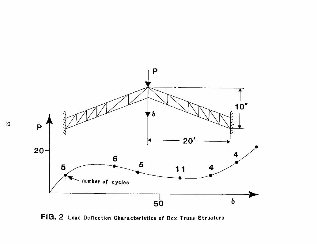
P
FIG, 2 Load Deflection Characteristics of Box Truss Structure


ELEMENT-BY-ELEMENT SOLUTION PROCEDURES
FOR NONLINEAR STRUCTURAL ANALYSIS
Thomas J.R. Hughes, James Winget and Itzhak Levit
Stanford University
SUMMARY
Element-by-element approximate factorization procedures are proposed for solv-
ing the large finite element equation systems which arise in nonlinear structuralmechanics. Architectural and data base advantages of the present algorithms overtraditional direct elimination schemes are noted. Results of calculations suggest
considerable potential for the methods described.
INTRODUCTION
Despite the attainment of significant increases in computer storage and speed
in recent years, many contemporary problems of engineering interest are simply too
complex to be solved with existing numerical algorithms and presently-available
hardware. In this paper we address the subject of solving the matrix equations
arising from finite element spatial discretizations. In Appendix I a brief sketch
is given of how finite element equation systems emanate from various classes of
structural mechanics problems. The matrix equations, though sparsely populated,
still entail enormous storage demands, especially in three-dimensional cases. This
is the major drawback to matrix-based ("implicit") finite element procedures. The
types of methods we have developed to deal with this circumvent the need to form
and factorize large global arrays. These methods have their origins in procedures
which pervade the numerical analysis literature. Basically, the idea is to replace
a large, complicated array by a product of simpler arrays. The original concepts
apparently emanate from the so-called "alternating direction (ADI) methods" (ref's.
6, 7, i0, 35). There is a large Russian literature on methods of this type whichis summarized in the books of Marchuk and Yanenko (ref's. 31 and 38, resp.). In
these works the terminologies used are the "method of fractional steps", the "split-
ting-up method", and the "method of weak approximation". In the field of computa-
tional aerodynamics these techniques are often described as "approximate factoriza-tion" methods (see e.g. Warming and Beam, ref. 37). The preceding references deal
primarily with finite difference methods in which the splitting is usually performedby decomposing a multi-dimensional partial differential operator into one-dlmension ....
al operators. This, of course, places geometrical and topological limitations on
the discretizations. Generally these methods are used most effectively in the con-
text of rectangular domains, or domains which are at least topologically equivalent
to rectangles. When circumstances like this prevail, very large problems can be
efficiently solved. Progress has been made in developing analogous finite element
s.
Work performed under Grant No. NAG 3-319
65
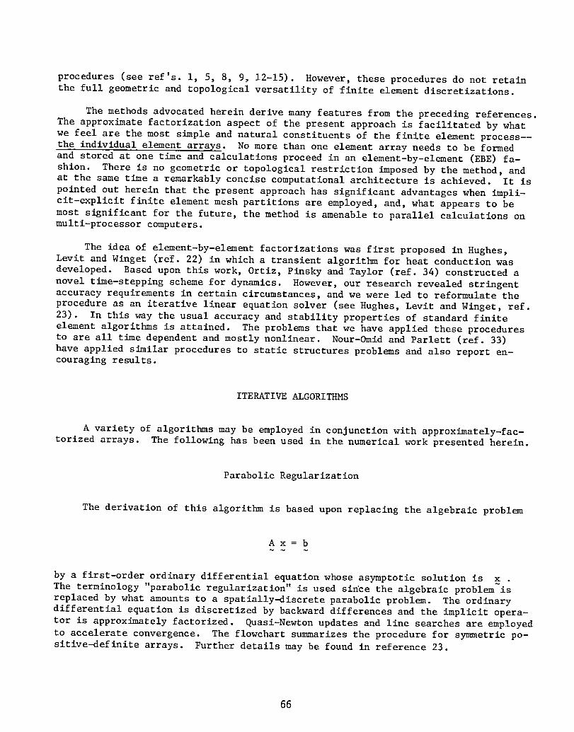
procedures (see ref's, i, 5, 8, 9, 12-15). However, these procedures do not retain
the full geometric and topological versatility of finite element dlscretizations.
The methods advocated herein derive many features from the preceding references.
The approximate factorization aspect of the present approach is facilitated by whatwe feel are the most simple and natural constituents of the finite element process--
the individual element arrays. No more than one element array needs to be formedand stored at one time and calculations proceed in an element-by-element (EBE) fa-
shion. There is no geometric or topological restriction imposed by the method, and
at the same time a remarkably concise computational architecture is achieved. It is
pointed out herein that the present approach has significant advantages when impli-
cit-explicit finite element mesh partitions are employed, and, what appears to be
most significant for the future, the method is amenable to parallel calculations on
multi-processor computers.
The idea of element-by-element factorizations was first proposed in Hughes,
Levit and Winger (re_. 22) in which a transient algorithm for heat conduction wasdeveloped. Based upon this work, Ortiz, Pinsky and Taylor (ref. 34) constructed a
novel time-stepping scheme for dynamics. However, our research revealed stringent
accuracy requirements in certain circumstances, and we were led to reformulate theprocedure as an iterative linear equation solver (see Hughes, Levit and Winget, ref.
23). In this way the usual accuracy and stability properties of standard finite
element algorithms is attained. The problems that we have applied these proceduresto are all time dependent and mostly nonlinear. Nour-Omid and Parlett (ref. 33)
have applied similar procedures to static structures problems and also report en-
couraging results.
ITERATIVE ALGORITHMS
A variety of algorithms may be employed in conjunction with approximately-fac-torized arrays. The following has been used in the numerical work presented herein.
Parabolic Regularization
The derivation of this algorithm is based upon replacing the algebraic problem
Ax=b
by a first-order ordinary differential equation whose asymptotic solution is x .The terminology "parabolic regularization" is used slnce the algebraic problem is
replaced by what amounts to a spatially-discrete parabolic problem. The ordinary
differential equation is discretized by backward differences and the implicit opera-
tor is approximately factorized. Quasi-Newton updates and line searches are employed
to accelerate convergence. The flowchart summarizes the procedure for symmetric po-
sitive-deflnite arrays. Further details may be found in reference 23.
66
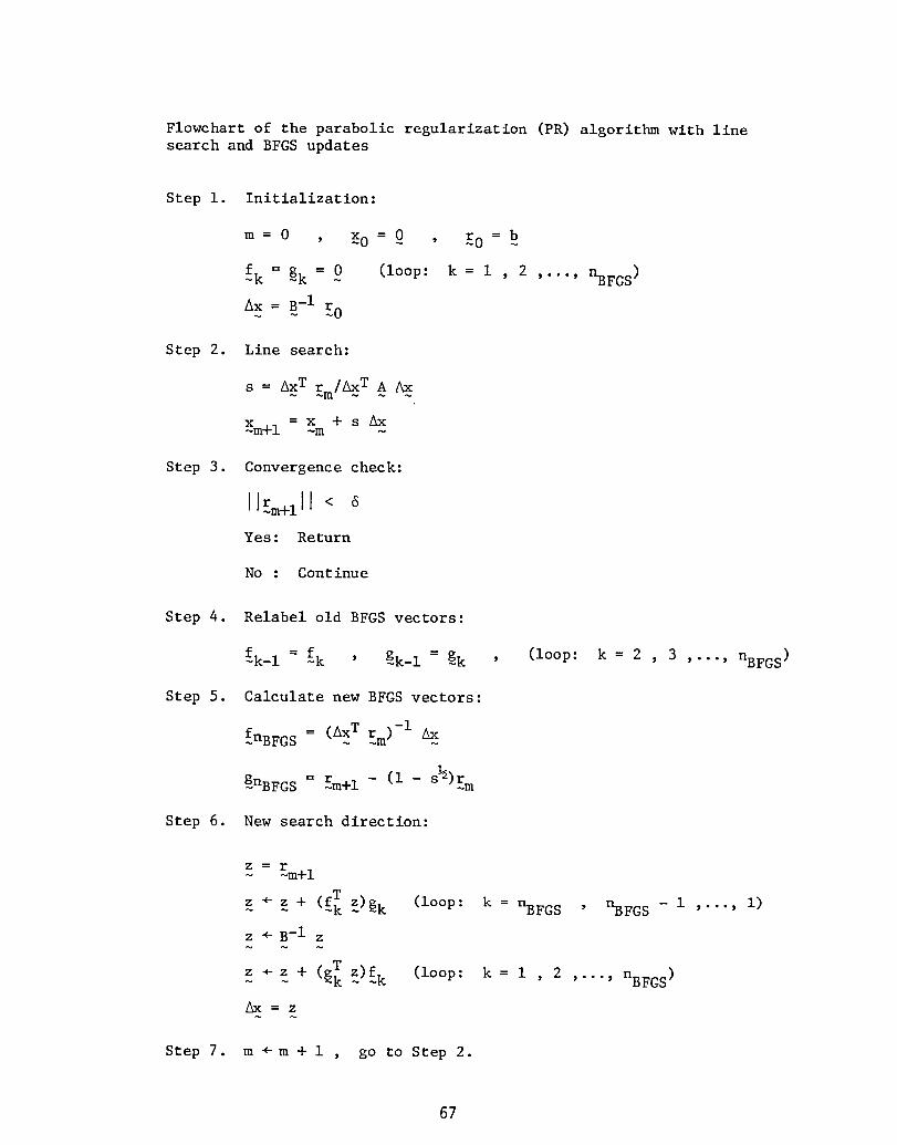
Flowchart of the parabolic regularization (PR) algorithm with linesearch and BFGS updates
Step i. Initialization:
m = 0 , _0 = ~0 , _0 = b~
_k = _k = ~0 (loop: k = i , 2 ,..., nBFGS )
A_ = B-I _0
Step 2. Line search:
s = AxT rm/AxT A Ax
=x +sAxXm+l ~m ~
Step 3. Convergence check:
llrm+lll <
Yes : Return
No : Continue
Step 4. Relabel old BFGS vectors:
_k-i : _k ' _k-i = _k ' (loop: k = 2 , 3 ,..., nBFGS)
Step 5. Calculate new BFGS vectors:
fnBFGS = (Axr rm )-I
_nBFGS = _m+l - (i - s½)rm
Step 6. New search direction:
z : rm+ I
z . z + (f_ z)gk (loop: k = nBFGS , nBFGS - i ,..., i)
z .B-I z
z .z + (g_ z)fk (loop: k = i , 2 ,..., nBFGS)
Ax=z
Step 7. m . m + i , go to Step 2.
67
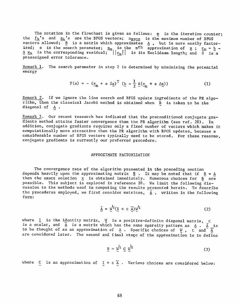
The notation in the flowchart is given as follows: m is the iteration counter;
the fk's and gk's are the BFGS vectors; nBFGS is the maximum number of BFGS
vectors allowed; B is a matrix which approximates A , but is more easily factor-
ized; s is the search parameter; _m is the mth approximation of _ ; _m = b -
_m is the corresponding residual; ][_m[[ is its Euclidean length; and _ is~apreassigned error tolerance.
Remark i. The search parameter in step 2 is determined by minimizing the potentialenergy
1 _(_m + s Ax)) (i)P(s) = - (_m + s Ax)T (b - _ ~
Remark 2. If we ignore the line search and BFGS update ingredients of the PR algo-rithm, then the classical Jacobi method is obtained when B is taken to be the
diagonal of A .
Remark 3. Our recent research has indicated that the preconditioned conjugate gra-
dients method attains faster convergence than the PR algorithm (see ref. 28). Inaddition, conjugate gradients requires only a fixed number of vectors which makes it
computationally more attractive than the PR algorithm with BFGS updates, because a
considerable number of BFGS vectors typically need to be stored. For these reasons,conjugate gradients is currently our preferred procedure.
APPROXIMATE FACTORIZATION
The convergence rate of the algorithm presented in the preceding section
depends heavily upon the approximating matrix B It may be noted that if B =
then the exact solution x is obtained immediately. Numerous choices for B arepossible. This subject is explored in reference 28. We limit the following dis-
cussion to the methods used in computing the results presented herein. To describethe procedures employed, we first consider matrices, A , written in the followingform:
= W=(I + E A)W a (2)
where I is the identity matrix, W is a positive-definite diagonal matrix,
is a scalar, and 6 is a matrix which has the same sparsity pattern as A . A is
to be thought of as an approximation of A . Specific choices of W , _~ and ~are considered later. The second and final stage of the approximation is to define
B : WI_C WI_ (3)
where C is an approximation of I + g A Various choices are considered below:
68

Two-component Splitting
Let A be decomposed as follows:
Then a possible definition of C is
C = (I + g AI)~ (I~+ g A--2)~ = I~+ g _~ + 2 AIA2 = I~+ _ A~ + O(E 2) (5)
The last par_t suggests the nature of the approximation. Computational simplicity is
gained if _i and _2 are very sparse and more easily factorized than A .
One-pass Multi-component Splitting
Consider a multi-component sum decomposition of A :
n
i=l
Let
n
c = n (!. _ Ai)~ i=l
= (I + S _i )(I + S _2 ) ... (I + g _n )
= I + g E + O(g 2) (7)~ ~
Clearly, this is just a straightforward generalization of the two-component splitting.
Two-pass Multi-component Splitting
This generalization of the preceding case has qualitative advantages under cer-
tain circumstances (Marchuk, ref. 31). Let
n i
Ei)EA.) ]I (I +-_c = _ (_+_~_ ~ ~i=l i=n
(cont'd .)
69

_I)(I+ _- __n) ×= (I +_ ~ _A 2) ... (I +_ ~
× + n_l)
= I + E: A'~+ 0(g2) (8)
If each _i is symmetric and positive semi-definite, then C is symmetric andpositive-definite. ~
Element-by-element (EBE) Approximate Factorizations
The EBE approximate factorization is simply a multi-component splitting inwhich the components are the finite element arrays themselves. That is we assume
ne_,
i=l
where _e is the eth element contribution to A . Then C may be defined byeither The one-pass or two-pass formulae, viz. ~ ~
ne£
c = _ (!+_e) (i0)~
e=l
ne£ i
E _e) H (I + _ _e) ("Marchuk EBE") (ii)c = H (!+_~ ~ ~i=l e=ne £
Remark i. We wish to use the term element in the generic sense of a "subdomain
model", where an element could be an individual finite element or a subassembly of
elements. Thus we allow limited assembly. Various equivalent terminologies havebeen used to define this concept, such as "substructures" and "superelements". Sub-
domain finite element models inherit the symmetry and definiteness properties of theglobal array. Consequently, the remark made after (8) applies.
Remark 2. Note that storage demands are vastly less in the EBE case. Only one
element at a time need be stored and processed. Whether or not it is desirable to
save factorized element arrays depends upon the availability of high speed RAM, andthe trade-off between CPU and disk I/O costs.
Remark 3. If elements are segregated into non-contiguous subgroups then calculations
are "parallelizable". For example, brick-like domains can be decomposed into eight
non-contiguous element groups (see fig. i). Because the elements in each subgroup
have no common degrees-of-freedom, they can be processed in parallel. The eight
groups, however, need to be processed sequentially. For analogous two-dimensional
domains, four element groups need to be employed. This feature has significant
70

computational implications for vector and multi-processor machines.
Remark 4. It has been our computational experience that if A is symmetric and
positive-definite, then qualitatively faithful approximate factorizations which
preserve these properties, such as (ii), perform much better than those that do not.
In the numerical examples presented herein we have employed (ii) exclusively.
Remark 5. In Reference 28 we have explored the use of reordering the element factors
and of approximately factorizing the individual element arrays. Preliminary results
indicate that significant improvements over the basic scheme of (ii) can be made.
SELECTION OF W , g AND A
In the computations presented herein the following definitions were employed:
W = diagonal entries of A (12)
= _ W-_ A W-½ (13)
Thus
= W + A (14)
This choice is motivated by the derivation of the PR algorithm (see ref. 23).
Remark I. A study performed by Nour-Omid and Parlett (ref. 33) indicates that the
following procedure, suggested by Winger, is superior:
= !W "½ (A - W)W -½ (15)
where W is given by (12). This leads to
= A (16)
Remark 2. The implicit-explicit element concept (see ref's. 20, 21, 24-27) has a very
simple and clean implementation within EBE approximate factorizations. Recall that
an explicit element contributes only its diagonal mass matrix to the coefficient ma-
trix A . Thus W , according to the preceding definition (i.e., eq. (12)), totallyaccounts for the explicit element contributions and the corresponding _e's are
identically zero. What this means is that explicit elements may be simply omitted
from the formula for C . In nonlinear problems this opens the way to time-adaptiveimplicit-explicit element partitions. In calculating the element contributions to
the residual (i.e. "b") a check can be made whether or not the critical time step isexceeded for the element. If it is not exceeded, a flag is set to indicate that ele-
ment contributions to C may be simply ignored. The potential savings in nonlinear
transient analysis procedures incorporating these ideas is clearly considerable.
71

SAMPLE PROBLEMS
The computed results were obtained on a VAX computer using single precision(32 bits per floating point word).
Elastic Cantilever Beam
The configuration analyzed is shown in figure 2. It represents one-half of a
plane strain beam modelled with 32 bilinear quadrilateral elements. A lumped mass
matrix was employed. The loading and boundary conditions are set in accord with an
exact, static linear elasticity solution (see pp. 35-39, ref. 36). However, here
the problem is forced dynamically. The beam is assumed initially at rest and all
loads are applied instantaneously at t = 0 + . In formulating the problem, the
Newmark algorithm is employed with B = _ and Y = ½ (see Appendix I). With these
parameters, unconditional stability is attained and no algorithmic damping is intro-duced (see ref's. Ii, 17, 21).
The numerical solution is dominated by response in the fundamental mode. This
is illustrated in figure 3. At a time step of AtA_E 2.5 x 10⁻⁴ an essentiallyexact solution is obtained. At a larger step of = 2.5 x i0-3 , a very crude
approximation of the response is obtained. It is interesting to relate the sizes of
these steps to the critical time step for explicit integration, Atcrit = hmin/C D =hmin/ _(% + 2H)/0 = 1.336 x 10⁻⁵ , and the approximate period of the fundamental
mode, T1 m .0122 (see table 1). As may be seen, both time steps are far outside therange of explicit integration. The larger time step resolves the fundamental mode
with only 5 steps, and thus is larger than the maximum feasible for this problem.
In comparing the results of the various methods it is important to keep in mindthat all methods give identical solutions.* Consequently, the primary basis of com-parison is the number of iterations needed to attain the solution. It was found
that the number of iterations per time step did not vary significantly from one time
step to another for a given method and specific step size. Results for the first
time step are presented in table 2. The following observations may be made: Ingeneral the element-by-element results are superior to Jacobi. Use of line search
and BFGS updates accelerate convergence. The best results are attained by the ele-
ment-by-element procedure with line search and BFGS updates.
It is somewhat surprising that methods (v) and (vi) converge faster at the
larger time step than at the smaller. At this point we have no explanation forthis phenomenon.
Elastic and Elastic-Perfectly Plastic Cantilever Beam
The geometrical definition of this problem is identical to the previous one
except that the entire beam is discretized by a 64 element mesh (the lower part of
the beam was added to the mesh of figure 2). The boundary conditions were changed
to the following.
The convergence tolerance, 6 in step 3 of the flowchart, was taken to be .0111bl I.
72
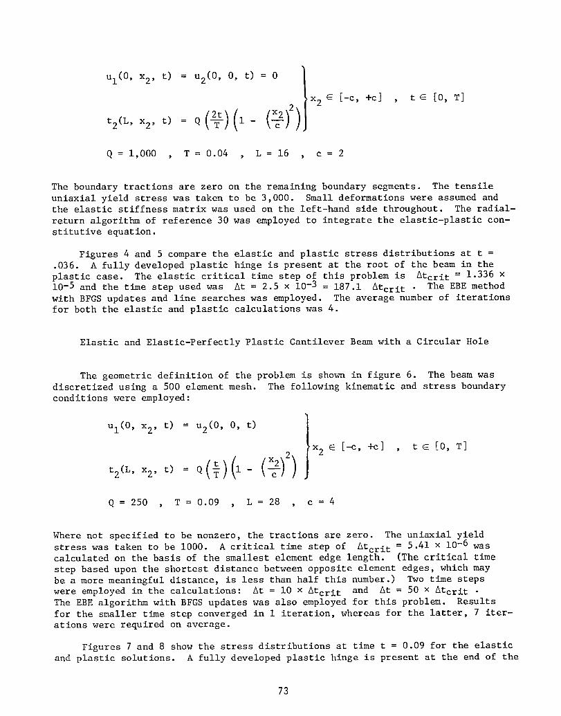
Ul(0, x2, t) = u2(0, 0, t) = 0 )Ix2 E I-c, +c] , t E [0, T]t2(L , x2, t) = Q (_)(i - (_)2
Q = 1,000 , T = 0.04 , L = 16 , c = 2
The boundary tractions are zero on the remaining boundary segments. The tensile
uniaxial yield stress was taken to be 3,000. Small deformations were assumed and
the elastic stiffness matrix was used on the left-hand side throughout. The radial-
return algorithm of reference 30 was employed to integrate the elastic-plastic con-
stitutive equation.
Figures 4 and 5 compare the elastic and plastic stress distributions at t =
.036. A fully developed plastic hinge is present at the root of the beam in the
plastic case. The elastic critical time step of this problem is Atcrit = 1.336 x
10-5 and the time step used was At = 2.5 x 10-3 = 187.1 Atcrit . The EBE method
with BFGS updates and line searches was employed. The average number of iterationsfor both the elastic and plastic calculations was 4.
Elastic and Elastic-Perfectly Plastic Cantilever Beam with a Circular Hole
The geometric definition of the problem is shown in figure 6. The beam was
discretized using a 500 element mesh. The following kinematic and stress boundary
conditions were employed:
Ul(O , x2, t) = u2(0 , 0, t) ]
Ix2 E I-c, +c] , t _ [0, T]2
Q = 250 , T = 0.09 , L = 28 , c = 4
Where not specified to be nonzero, the tractions are zero. The uniaxial0Yieldlbstress was taken to be i000. A critical time step of Atcrit = 5.41 x - wascalculated on the basis of the smallest element edge length. (The critical time
step based upon the shortest distance between opposite element edges, which maybe a more meaningful distance, is less than half this number.) Two time steps
were employed in the calculations: At = i0 x Atcrit and At = 50 x Atcrit
The EBE algorithm with BFGS updates was also employed for this problem. Results
for the smaller time step converged in i iteration, whereas for the latter, 7 iter-
ations were required on average.
Figures 7 and 8 show the stress distributions at time t = 0.09 for the elastic
and plastic solutions. A fully developed plastic hinge is present at the end of the
73

beam and a secondary plastic hinge has partially developed in the stress concentra-
tion zone (plastic regions are shown dashed in fig. 8c).
We wish to remark upon the contour-line routine used to obtain the results
presented in this section. The finite element analyzer calculates the stresses at
the integration points. The data is then extrapolated to the nodal points by means
of a weighted average of all the integration points in the interior domains of all
elements connected to the nodal point. The weights are taken as the inverse of the
distance between the integration point and the nodal point. This type of data
smoothing ensures that the values obtained at the nodal points will be bounded bythe data calculated at the integration points which is an essential property when
plastic stresses are present and ensures continuity of stress contours between ele-
ment domains. However, this method has some drawbacks. For example, data which is
anti-symmetric about the neutral axis of the beam, such as _ii , will result inlinear distribution of contour lines in all elements having the center line as partof their boundary even in the case where these elements have a uniform stress dis-
tribution (part of a plastic hinge). Data with symmetry with respect to the neutral
axis, such as the von Mises stress, does not suffer from this type of smoothing.
CONCLUDING REMARKS
In this paper EBE approximate factorization techniques have been proposed and
compared on test problems. The PR algorithm with BFGS updates performed well, how-
ever, the need to store BFGS vectors is considered a significant disadvantage, and
thus the fixed storage requirements and improved convergence characteristics of the
conjugate gradients algorithm renders it preferable (ref. 28). Improved behavior
has also been attained in reference 28 by employing reorderings of the element fac-tors.
It should be kept in mind that the EBE concept has been explored herein as a
finite element, linear equation solving procedure. Although initial attempts at
directly using EBE ideas to develop time stepping algorithms had some deficienciesit may still ultimately prove profitable to couple EBE concepts with the time-step-
ping loop and even the nonlinear iterative loop. It is interesting to note that the
multigrid method found its initial success as a linear equation solver, but in the
most recent and successful variants the multigrid philosophy permeates all aspects
of the methodology (see Brandt, ref. 4).
A step has been taken in the development of EBE solution of finite element equa-
tion systems. A considerable potential exists for the technique, but much research
still remains to be done to bring the methods to fruition.
APPENDIX I - DERIVATION OF LINEAR ALGEBRAIC SYSTEMS IN THE FINITE ELEMENT
ANALYSIS OF NONLINEAR MECHANICS PROBLEMS
Semi-discrete Equations of Nonlinear Mechanics
Consider the following semi-discrete system
74

M a = F (I.I)
where M , a and F represent the (generalized) mass matrix, acceleration vector
and force vector, respectively. Equation (I.i) may be thought of as arising from a
finite element discretization of a solid, fluid, structure or combined system. In
general, M , a and F each depend on time (t) . Explicit characterization of
M , a and F may be given for particular systems under consideration.
Nonlinear Structural and Solid Mechanics
In nonlinear structural and solid mechanics the Lagrangian kinematical descrip-
tion is frequently adopted. In this case the important kinematical quantities are
, the material-particle displacement from a reference configuration; v = d ,the particle velocity; and a = v = d , the particle acceleration. Dots~indicate
the Lagrangian time-derivative in which the material particle is held fixed. Theforces are assumed to take the form
F = Fext - N (1.2)~
where Fext is the vector of given external forces and N denotes the vector ofinternal forces, which may depend upon d , d and their histories. To make the
dependence precise, one need introduce equations whi_ _efi-_e t-_e_onstitutive (i.e.
stress-deformation) behavior of the materials in question. These equations vary
widely in type and complexity. For example, they may be algebraic equations, dif-
ferential equations or integro-differential equations. In addition, inequality
constraints may be present, such as in plasticity theory.
Time Discretization
To solve the semi-discrete problem, a time-discretization algorithm needs to be
introduced. For purpose of illustration we shall employ the Newmark family of meth-ods (ref. 32). Generalization to other time integrators, such as the Hilber-Hughes-
Taylor algorithm (ref.'s. 16, 18, 19, 21) which possesses improved properties, may
be easily facilitated without essential alteration to the following formulation.
The Newmark "predictors" are given by
At2 (I.3)_n+l = _n + At _n + 2 (i - 2_)an
_n+l = Vn + At (i - y)a n (1.4)
where subscripts refer to the step n.umber; At is the time step; _n ' Xn and _n
are the approximations to d(t n) , d(tn) and d(tn) , respectively; and B andy are parameters which govern the accuracy and stability of the method (ref's. ii,
17, 29).
75

Calculations commence with the given initial data (i.e., dO and v0) and a0which may be calculated from
= _ext _ _0 (I.5)[0
if M is diagonal, as is common in structural dynamics, the solution of (I.5) is
rendered trivial. Otherwise, a factorization, forward reduction and back substitu-
tion are necessary to obtain _0 "
In the sequel we are only interested in members of the Newmark family for whichB > 0 .
In each time step a nonlinear algebraic problem arises which may be solved by
Newton-Raphson and quasi-Newton-type iterative procedures. There are several ways
of going about this. In the following implementation an algebraic problem is formu-
lated in which acceleration increments are the unknowns. This form of the implemen-tation is useful in that disparate field theories, such as fluid mechanics and heat
conduction, may be formally considered as special cases.
Acceleration Formulation
i = 0 (i is the iteration counter) (I.6)
d(i) ~~n+l = _n+l (I.7)
(i) ~Vn+ I = Vn+ I _ (predictor phase) (1.8)
a"i'(_ = 0 (I 9)~n+l ~
_ext (i) •(i) (i)R = _'n+l- Nn+l - _In+lan+l (residual, or out-of-balance, force) (I.i0)
* (i) _(i) .(i)M = _n+l + ¥At _n+l + 8At2 (effective mass) (I.ii)~ _n+l
M* Aa = R (1.12)
a(i+l) (i)~n+l = _n+l + Aa (1.13)
(i+l) (i)
in+l = !n+l + yAt Aa (corrector phase) (1.14)
d(i+l) _(i)
n+l = _n+l + _At2 Aa (1.15)
76
If additional iterations are to be performed, i is replaced by i+l , and
calculations resume with (I.10). Either a fixed number of iterations may be per-
formed, or iterating may be terminated when Aa and/or R satisfy preassigned
convergence conditions. When the iterative phase is completed, the solution atd(i+l) _ (i+l)step n+l is defined by the last iterates (viz. dn4-] = n_] ; Vn+l = Zn+l ;
(i+l] .........and a_±1 = a _I o ). At this point, n is replacedby n+l , and calculations_ LLT.I. _ -i-.L.
for the next _ime step may begln.
In practice, dn , vn and an are generallysaved during the iterativephase.(i+l) ~ oii+l) _ii+l) ma_ be computedas needed,on thealong with en+l ; but Zn+l and _n+l
elementlevel.
The matrices C and K are the tangent damping and tangent stiffness matrices,
respectively. These are linearized operators associated with N . For example, if
is an algebraic function of d and d , then
= _N/_d (I.16)
and
= aNla_ (I.17)
Generally in structural and solid mechanics, M , K and C are symmetric,
M and K are positive-definite, and C is positive semi-definite.
So-called implicit-explicit mesh partitions (ref's. 2, 3, 20, 21, 24-27) may
be encompassed by the above formulation simply by excluding explicit element/nodecontributions from the definitions of C and K . A totally explicit formulation
is attained by ignoring C and K . In these cases it is necessary to employ adiagonal mass matrix in explicit regions to attain full computational efficiency.
It may be observed that the preceding algorithm may be specialized to nonlinearstatics and linear dynamics and statics:
Nonlinear Statics
In this case ignore M and C and set v and a to zero throughout.
Linear Dynamics
In this case M , C and K are constant and
N = C v + K d (I.18)
Linear Statics
In this case ignore M and C , set v and a to zero throughout, K isconstant and
77
N = K d (1.19)
To simplify the writing in the body of this paper we adopt the following nota-tions in place of (1.12):
A x = b (1.20)
Thus during each step, at each iteration, we wish to solve (1.28) in which A isassembled from element arrays, that is ~
ne%
A = _ Ae (I.21)e=l
REFERENCES
1. Baker, A. J., "Research on a Finite Element Algorithm for the Three-dimensional
Navier-Stokes Equations," AFWAL-TR-82-3012, Wright-Patterson Air Force Base,Ohio, 1982.
2. Belytschko, T., and Mullen, R., "Mesh Partitions of Explicit-Implicit Time
Integration," Formulations and Computational Algorithms in Finite Element Anal-
ysis, Eds. K. J. Bathe et al., M.I.T. Press, Cambridge, Massachusetts, 1977.
3. Belytschko, T., and Mullen, R., "Stability of Explicit-Implicit Mesh Partitions
in Time Integration," International Journal for Numerical Methods in Engineering,Vol. 12, No. i0, 1575-1586 (1979).
4. Brandt, A., "Guide to Multigrid Development," in Multigrid Methods (W. Hackbusch
and U. Trottenberg, eds.) Springer-Verlag, Berlin-Heidelberg-New York, 1982.
5. Dendy, J. E., and Fairweather, G., "Alternating-direction Galerkin Methods for
Parabolic and Hyperbolic Problems on Rectangular Polygons," SIAM J. Numer. Anal.,Vol. 2, 144-163 (1975).
6. Douglas, J., "On the Numerical Integration of Uxx + Uyy = ut by Implicit Meth-ods," J. Soe. Indust. Appl. Math., Vol. 3, 42-65 (1965).
7. Douglas, J., "Alternating Direction Methods for Three Space Variables," Numer.Math., 4, 41-63 (1962).
8. Douglas, J., and Dupont, T., "Galerkin Methods for Parabolic Equations," SIAMJ. Numer. Anal., Vol. 7, 575-626 (1970).
9. Douglas, J., and Dupont, T., "Alternating-direction Galerkin Methods on Rec-
tangles," pp. 133-214 in Proceedings Symposium on Numerical Solution of PartialDifferential Equations, II, B. Hubbard (ed.), Academic Press, New York, 1971.
78
i0. Douglas, J., and Rachford, H. H., "On the Numerical Solution of Heat Conduction
Problems in Two and Three Space Variables," Trans. Amer. Math. Soc., Vol. 82,
421-439 (1956).
ii. Goudreau, G. L., and Taylor, R. L., "Evaluation of Numerical Integration Methods
in Elastodynamics," Computer Methods in Applied Mechanics and Engineering, Vol.2, 69-97 (1972).
12. Hayes, L. J., "A Comparison of Alternating-direction Collocation Methods for
the Transport Equation," pp. 169-177 in New Concepts in Finite Element Analysis,
AMD Vol. 44, (T.J.R. Hughes et al. eds.), ASME, New York, 1981.
13. Hayes, L. J., "Finite Element Patch Approximations and Alternating-Direction
Methods," Mathematics and Computers in Simulation, Vol. XXII, 25-29 (1980).
14. Hayes, L. J., "Implementation of Finite Element Alternating-Direction Methods
on Nonrectangular Regions," International Journal for Numerical Methods in Engi-neering, Vol. 16, 35-49 (1980).
15. Hayes, L. J., "Galerkin Alternating-Direction Methods for Nonrectangular Regions
Using Patch Approximations," SIAM J. Numer. Anal., Vol. 18, No. 4, 627-643 (1981).
16. Hibbitt, H. D., and Karlsson, B. I., "Analysis of Pipe Whip," ASME Paper No.
79-PVP-122, presented at the Pressure Vessels and Piping Conference, San Fran-
cisco, California, June 25-29, 1979.
17. Hilber, H. M., Analysis and Design of Numerical Integration Methods in Struc-
tural Dynamics, Report No. EERC76-29, EarthquakeEngineering Research Center,
University of California, . Berkeley, California, November 1976.
18. Hilber, H. M., and Hughes, T.J.R., "Collocation, Dissipation, and 'Overshoot'
for Tim_ Integration Schemes in Structural Dynamics," Earthquake Engineering
and Structural Dynamics, Vol. 6, 99-118 (1978).
19. Hilber, H. M., Hughes, T.J.R., and Taylor, R. L., "Improved Numerical Dissipa-tion for Time Integration Algorithms in Structural Dynamics: Earthquake Engi-
neering and Structural Dynamics, Vol. 5, 283-292 (1977).
20. Hughes, T.J.R., "Implicit-explicit Finite Element Techniques for Symmetric and
Non-symmetric Systems," pp. 255-267 in Recent Advances in Non-linear Computa-
tional Mechanics, (eds. E. Hinton, D.R.J. Owen and C. Taylor)Pineridge Press,
Swansea, U.K., 1982.
21. Hughes, T.J.R., "Analysis of Transient Algorithms with Particular Reference
to Stability Behavior," Computational Methods in Transient Analxsis, (eds. T.Belytschko and T.J.R. Hughes), North-Holland Publishing Co., Amsterdam, 1983.
22. Hughes, T.J.R., Levit, I., and Winger, J., "Implicit, Unconditionally Stable,
Element-by-element Algorithms for Heat Conduction Analysis," Journal of the Engi-neering Mechanics Division, ASCE, April 1983.
23. Hughes, T.J.R., Levit, I., and Winget, J., "An Element-by-element Solution
Algorithm for Problems of Structural and Solid Mechanics," Computer Methods in
Applied Mechanics and Engineering, 241-254, Vol. 36, No. 2 (1983).
79
24. Hughes, T.J.R., and Liu, W. K., "Implicit-Explicit Finite Elements in Transient
Analysis: Stability Theory," Journal of Applied Mechanics, Vol. 45, 371-374(1978).
25. Hughes, T.J.R., and Liu, W. K., "Implicit-Explicit Finite Elements in Transient
Analysis: Implementation and Numerical Examples," Journal of Applied Mechanics,Vol. 45, 375-378 (1978).
26. Hughes, T.J.R., Pister, K. S., and Taylor, R. L., "Implicit-Explicit Finite
Elements in Nonlinear Transient Analysis," Computer Methods in Applied Mechanicsand Engineering, Vols. 17/18, 159-182 (1979).
27. Hughes, T.J.R., and Stephenson, R. A., "Convergence of Implicit-Explicit Algo-rithms in Nonlinear Transient Analysis," International Journal of Engineering
Science, Vol. 19, No. 2, 295-302 (1981).
28. Hughes, T.J.R., Winget, J., Levit, I., and Tezduyar, T. E., "New Alternating
Direction Procedures in Finite Element Analysis based upon EBE Approximate Fac-
torizations," Proceedings of the Symposium on Recent Developments in ComputerMethods for Nonlinear Solid and Structural Mechanics (eds. N. Perrone and S.Atluri) ASME AMD Volume, June 1983.
29. Krieg, R. D., and Key, S. W., "Transient Shell Response by Numerical Time Inte-
gration," International Journal for Numerical Methods in Engineering, Vol. 7,273-286 (1973).
30. Krieg, R. D., and Krieg, D. B., "Accuracies of Numerical Solution Methods for
the Elastic-Perfectly Plastic Model," Journal of Pressure Vessel Technology,510-515, November 1977.
31. Marchuk, G. I., Methods of Numerical Mathematics, Springer-Verlag, New York-Heidelberg-Berlin, 1975.
32. Newmark, N. M., "A Method of Computation for Structural Dynamics," Journal of
the Engineering Mechanics Division, ASCE, 67-94 (1959).
33. Nour-Omid, B., and Parlett, B. N., "Element Preconditioning," Report PAM-103,
Center for Pure and Applied Mathematics, University of California, Berkeley,October 1982.
34. Ortiz, M., Pinsky, P. M., and Taylor, R. L., "Unconditionally Stable Element-by-
element Algorithms for Dynamic Problems," Computer Methods in Applied Mechanicsand Engineering, 223-239, Vol. 36, No. 2 (1983).
35. Peaceman, D. W., and Rachford, H. H., "The Numerical Solution of Parabolic and
Elliptic Differential Equations," J. Soc. Indust. Appl. Math., Vol. 3, 28-41(1955).
36. Timoshenko, S., and Goodier, J. N., Theory of Elasticity, Second Edition, McGraw-Hill, New York, 1951.
37. Warming, R. F., and Beam, R. M., "On the Construction and Application of Impli-
cit Factored Schemes for Conservation Laws," SIAM-AMS PROCEEDINGS, Vol. ii, 85-129 (1978).
8O

38. Yanenko, N. N., The Method of Fractional Steps, Springer-Verlag, New York-Heidelberg-Berlin, 1971.
Table i Comparison of time steps used incalculations with characteristic
time scales.
At 2.5 x 10⁻⁴ 2.5 x 10 -3
At 18.71 187.1Atcrit
T1 48.9 4.89At
Table 2 Number of iterations required for convergence
for the problem illustrated in Figure 2.
__ At 2.5 x 10⁻⁴ 2.5 × 10⁻³
Method __ (= 18.71 atcrit ) (= 187.1 Atcrit)
(i) Jacobi 99 _(i)
(ii) Jacobi + LS 38 75
(iii) Jacobi + LS + BFGS 15 21
(iv) EBE 14 16
(v) EBE + LS 9 6
(vi) EBE + LS + BFGS 5 4
Key: LS = line search
EBE = element-by-element
Note: (i) No convergence attained after 150 iterations.
81

F3 4 3 4
1 2 1 2 F
3 4 3 4
1 2 1 2
Figure 1. Decompostion of three-dimensional domain into eightgroups of brick elements for parallel processing.
X2
k L .!tl =PLx2/I A= 1.2 × 10⁶
- P_ p=.8 X 108t=- P(c=-x_=)/(21) 1ooo
I = 2cS/3 I P= .002o _ t L=16
C=2
x'node A
25 20 27 28 29 80 31 3217 18 19 20 21 22 23 24
9 10 11 12 13 14 16 16
x!
Figure 2. Problem definition and finite element mesh
82

a. E_ast_€Sotut_on
_. _sttc So|utton
D, plastic: Solutloft
_. p_sstl=sol.t_on F_re 5. _on _ises Stress
F_tre 4. stress _ _

Y
r
4.
x
., 28.
a. GeometryDeflnlllon
ooP,= 1200000.
p = 800000.
oy= 1000.
b. Flnllo Element Mesh
Figure 6.
Time =0.09 .1/l _ Tlme = 0.09
A - -2250.00 el - -1200.00
,_ , 0 - 0.00 .'-_[ _.........,,..----- 0 0.00r" - 75Q.0Q [ " "00-00
€-,....._ F - 1500.00 F 8QQ.00G - 2250.00. ; 1200.00
eL. Axial Stress o_1 8. Axial Stress 0"11
R- 250.00
8 - 500.O0 A - 200.00
_'_'-_"_'__.___N___'2_"_ _ ,_._ _- _._,.-:.__.,._, ,-- o looo.oo -_ c- 6oo.oo,oo.oo .o_o.oo'_"-,,...,.. r ISQO.O0 [ - IOQO.°O___ "_.--o"_ "_ _ zTso.oo
H - 2CX_O.
c. Von Mises Stress c. Von Mises Stress
Figure 7. Stress Distribution Figure 8. Stress Distribution(elastic solution) (plastic solution)
84
AutomaticFinite ElementGenerators
Paul S. Wang*
Departmentof MathematicalSciencesKent State University
Kent, Ohio 44242
The design and implementation of a software system forgenerating finite elements and related computations aredescribed. Exact symbolic computational techniques areemployed to derive strain-displacement matrices and elementstiffness matrices. Methods for dealing with the exces-sive growth of symboiic expressions are discussed.Automatic FORTRAN code generation is described withemphasis on improving the efficiency of the resultant code.
i. Introduction
Recent years have seen increasing interest in using computer-basedsymbolic and algebraic manipulation systems for computations in bothlinear and nonlinear finite element analysis. Application areasinclude the symbolic derivation of stiffness coefficients [ref. i],[ref. 2], the reduction of tedium in algebraic manipulation, the gen-eration of FORTRAN code from symbolic expressions [ref. 3], [ref. 4]etc. The benefits and usefulness of such an approach in engine struc-ture research are evident. However, several problems need be solvedbefore this approach can become widely accepted and practiced:
(i) the efficiency of the symbolic processor and its ability to handlethe large expressions associated with practical problems.
(ii) the interface between a symbolic system and a finite element sys-tem on the same computer, and
(ill)the inefficiencies that are usually associated with automaticallygenerated code.
The MACSYMA system [ref. 5] is a highly sophisticated computersystem for performing exact symbolic mathematical computations. It
*Work reported herein has been supported in part by NASA under GrantNAG3-298.
85
provides many high-levelcommands for symboliccomputationsuch as dif-ferentiation, matrix multiplication and matrix inverse. MACSYMA isdevelopedat the MassachusettsInstituteof Technologyand has recentlybeen made available on the VAX-II/780 computer which is an affordablehigh-performanceminicomputer with a very large address space. Theversion of MACSYMA on the VAX under the UNIX operationsystem [ref.6]is known as VAXIMA [ref.7].
We describe our on-going research on the design and implementationof a finite element generator running under the VAXIMA system and ourexperience, so far, in dealing with the problems mentioned earlier.
2. _ specifications and _I_
The finite element generator (Generator)as a software systemshould provide a set of predefined functionalitiesand be constructedin such a way as to exhibit prescribed characteristics. These func-tional specifications and design goals will then guide the detailedprogram design and implementationof the software system.
From a functional point of view, the Generator will perform thefollowing:
(i) to assist the user in the symbolicderivationof finite elements;
(2) to provide routines for a variety of symbolic computationsin fin-ite element analysis, includinglinear and non-linearapplicationsespeciallyfor shells [ref.8];
(3) to provide easy to use interactivecommands for most common opera-tions;
(4) to allow the mode of operation to range from interactivemanualcontrol to fully automatic;
(5) to generate, based on symbolic computations, FORTRAN code in aform specifiedby the user;
(6) to automatically arrange for generated FORTRAN code to compile,link and run with FORTRAN-basedfinite element analysis packagessuch as the NFAP package [ref.9];
(7) to provide for easy verification of computational results andtesting of the code generated.
In providing the above functions attention must be paid to makingthe system easy to use, modify and extend. Our initial effort isfocused on the isoparametricelement family. Later the system can beextended to a wider range of finite elements.
86
_. Generationof element _ !R_
Symbolicprocessingcan play a very important role in the genera-tion of element matrices, especially for higher order elements. As anexample, we shall describe the automatic processing leading to thederivation of the elment stiffnessmatrix [K] in the isoparametricfor-mulation. From user supplied input information such as the elementtype, the number of nodes, the nodal degrees of freedom, the displace-ment field interpolationpolynomial and the material propertiesmatrix[D], the Generator will derive the shape functions, the strain-displacementmatrix [B] and the element stiffnessmatrix [K].
The computationis divided into five logical phases (fig. I) eachis implementedas a LISP program module running under the VAXIMA sys-tem. Aside from certain interface considerations,these modules arequite independent and can therefore be implemented and testedseparately. This allows different people to work on differentmodulesat the same time. After the modules are individuallytested then theycan be integratedand verified together. Any problems can be isolatedto a module and fixed quickly. Detailed descriptionof these phasesfollows.
i.l. Phasel : defineiipm_imlame.2ms_
The task of this phase is to interact with the user to define allthe input names, variables,and values that will be needed later. Thebasic input mode is interactivewith the system prompting the user atthe terminal for needed input information. While the basic input modeprovides flexibility,the input phase can be tedious. Thus we alsoprovide a menu-driven mode where well-known element types togetherwith their usual parametervalues are pre-definedfor user selection.Afully user-friendlyinput phase is a goal of our system.
The input handling features planned include :
(i) free format for all input with interactive prompting showing thecorrect input form;
(2) editing capabilitiesfor correctingtyping errors;
(3) the capabilityof saving all or part of the input for use later;
(4) the flexibilityof receiving input either interactivelyor from atext file.
_.2. Phase II : _ and [B] matrix computation
The strain-displacementmatrix [B] is derived from symbolicallydefined shape functions in this phase. Let n be the number of nodesthen
H = (hi h2, hn), ---f
is the shape functionvector whose componentsare the n shape functionshI through hn. The value for the shape functionswill be derived in a
87
later phase. Here we simply compute with the symbolic names. Let r,sand t be the natural coordinates in the isoparametric formulation andHP be a matrix
I H'r ]
HP = H,s
H,t
where H,r stands for the partial derivative of H with respect to r.The Jacobian J is then
J = HP . [x,y,z]
where x stands for the column vector [Xl,..., Xn] etc. Now theinverse, in full symbolic form, of J can be computed as
j-i = invjdet(J)
By forming the matrix (invj . HP) we can then form the [B] matrix.
3.3. h£hg_s_III: m!m/ll tL n
Based on the interpolation polynomials and nodal coordinates theshape function vector H is derived and expressed in terms of thenatural coordinates r.s and t in the isoparametric formulation. Thusthe explicit values for all hi and all their partial derivatives withrespect to r,s and t, needed in HP are computed here.
3.4. Phase IV: FORTRAN code _ for [B]
A fortran subroutine for the numerical evaluation of the strain-displacement matrix [B] is generated for use with the NFAP package.This NFAP package is a large FORTRAN based system for linear and non-linear finite element analysis• It is developed and made available tous by P. Chang of the University of Akron. It has been modified andmade to run in FORTRAN 77 under UNIX.
Assignment statements will be generated to define the componentsof the shape function vector H and the various partial derivatives.These variables are then used in assigning values to the FORTRAN arraycorresponding to [B]. FORTRAN code generation is controlled by a "tem-plate" file which is a skeleton FORTRAN program with special instruc-tions for code generation•
Details of the FORTRAN code generator will be discussed later.
3.5. Phase V : _ and generate FORTRAN code for [K]
The inverse 6f the Jacobian, J, appears in [B]. By keeping theinverse of J as INVJ/det(J), the quantity det(J) can be factored from[B] and, denoting by [BJ] the matrix [B] thus reduced, we have
f [Bj]T [D] [BJ][K] = det(J) dr ds dt
88
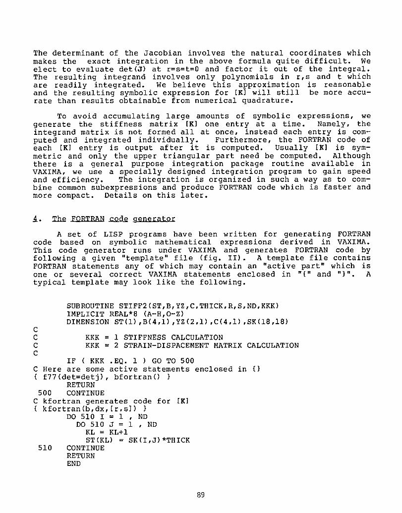
The determinant of the Jacobian involves the natural coordinates which
makes the exact integration in the above formula quite difficult. Weelect to evaluate det(J) at r=s=t=0 and factor it out of the integral.The resulting integrand involves only polynomials in r,s and t whichare readily integrated. We believe this approximation is reasonableand the resulting symbolic expression for [K] will still be more accu-rate than results obtainable from numerical quadrature.
To avoid accumulating large amounts of symbolic expressions, wegenerate the stiffness matrix [K] one entry at a time. Namely, theintegrand matrix is not formed all at once, instead each entry is com-puted and integrated individually. Furthermore, the FORTRAN code ofeach [K] entry is output after it is computed. Usually [K] is sym-metric and only the upper triangular part need be computed. Althoughthere is a general purpose integration package routine available inVAXIMA, we use a specially designed integration program to gain speedand efficiency. The integration is organized in such a way as to com-bine common subexpressions and produce FORTRAN code which is faster andmore compact. Details on this later.
4. The FORTRAN code generator
A set of LISP programs have been written for generating FORTRANcode based on symbolic mathematical expressions derived in VAXIMA.This code generator runs under VAXIMA and generates FORTRAN code byfollowing a given "template" file (fig. II). A template file containsFORTRAN statements any of which may contain an "active part" which isone or several correct VAXIMA statements enclosed in "{" and "}". A
typical template may look like the following.
SUBROUTINE STIFF2(ST,B,YZ,C,THICK,R,S,ND,KKK)IMPLICIT REAL*8 (A-H,O-Z)DIMENSION ST(l) ,B(4,1) ,YZ(2,1) ,C(4,1) ,SK(18,18)
CC KKK = 1 STIFFNESS CALCULATIONC KKK = 2 STRAIN-DISPACEMENT MATRIX CALCULATIONC
IF ( KKK .EQ. 1 ) GO TO 500C Here are some active statements enclosed in {}
{ f77(det=detj), bfortran() }RETURN
500 CONTINUE
C kfortran generates code for [K]{ kfortran(b,dx,[r,s]) }
DO 510 I = 1 , NDDO 510 J = 1 , ND
KL = KL+IST(KL) = SK(I,J)*THICK
510 CONTINUERETURNEND
89
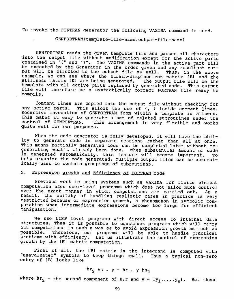
To invoke the FORTRAN generator the following VAXIMA command is used.
GENFORTRAN (templ ate- f il e-name, output- fil e-name)
GENFORTRAN reads the given template file and passes all charactersinto the output file without modification except for the active partscontained in "{" and "}". The VAXIMA commands in the active part willbe executed by the Generator in the order given and any resultant out-put will be directed to the output file as well. Thus, in the aboveexample, we can see where the strain-displacement matrix [B] and thestiffness matrix [K] are being generated. The output file will be thetemplate with all active parts replaced by generated code. This outputfile will therefore be a syntactically correct FORTRAN file ready tocompile.
Comment lines are copied into the output file without checking forany active parts. This allows the use of {, } inside comment lines.Recursive invocation of GENFORTRAN from within a template is allowed.This makes it easy to generate a set of related subroutines under the
control of GENFORTRAN. This arrangement is very flexible and worksquite well for our purposes.
When the code generator is fully developed, it will have the abil-ity to generate code in separate sessions rather than all at once.This means partially generated code can be completed later without re-generating what's already been done. When substantial amount of codeis generated automatically, this feature will become important. Tohelp organize the code generated, multiple output files can be automat-ically used to contain groupings of subroutines.
and of FORTRAN code
Previous work in using systems such as VAXIMA for finite elementcomputation uses user-level programs which does not allow much controlover the exact manner in which computations are carried out. As aresult, the ability of handling realistic cases in practice is veryrestricted because of expression growth, a phenomenon in symbolic com-putation when intermediate expressions become too large for efficientmanipulation.
We use LISP level programs with direct access to internal data
structures. Thus it is possible to construct programs which will carryout computations in such a way as to avoid expression growth as much aspossible. Therefore, our programs will be able to handle practicalproblems with efficiency. Let us illustrate the control of expressiongrowth by the [K] matrix computation.
First of all, the [B] matrix in the integrand is computed with"unevaluated" symbols to keep things small. Thus a typical non-zeroentry of [B] looks like
hr 2 hs . y - hr . y hs 2
where hr 2 = the second component of H,r and y = [yl,...,yn]. But these
90

symbols remain un-evaluated at this point. As stated before, weproceed to generate the entries of [K] one at a time to keep expres-sions small. In doing this, we apply the formula
[K]=i__ /[B]iT [D]ij [B]j dV
to collect terms with respect to [D].. Coefficients thus obtainedare kept in un-expanded form on a lis_which is consulted for dupli-cates whenever a new coefficientis generated. This identifiescommon(duplicate)subexpressions in different entries of [K] and keep theresultingFORTRAN code compact and more efficient. When a new coeffi-cient is formed then it is evaluated and expressed as a polynomialinvolving the natural coordinates r,s and t. Now a special-purposeintegration routine is used. The integrationresult for each coeffi-cient is converted into FORTRAN code and assigned to a temporary FOR-TRAN variable. Thus a typical section of the code for [K] may looklike the following.
t30 = -((16*y3-4*y2-12*yl)*y4+(-12*y2-4*yl)*y31 +4*y2**2+8*yl*y2+4*yl**2)/3.0t31 = ((16*x3-4*x2-12*xl)*y4+(-12*x3+4*x2+8*xl)*y2
1 +(-4*x3+4*xl)*yl)/3.0t32 = ((16*x4-12*x2-4*xl)*y3+(-4*x4+4*x2)*y21 +(-12*x4+8*x2+4*xl)*yl)/3.0t33 = -((16*x3-4*x2-12*xl)*x4+(-12*x2-4*xl)*x31 +4*x2**2+8*xl*x2+4*xl**2)/3.0k(5,7) = 4*(d6*t33+d3*(t32+t31)+dl*t30)/detkk(5,8) = 4*(d5*t33+d6*t32+m2*t31+d3*t30)/detk
In the above, t30 etc. are the temporary variables and dl,d2 etc. areentries of the material propertiesmatrix [D]. Without the techniquesmentioned here, the code for each single [K] entry will require 5 to 8continuationcards (for a plane 4-node element).
Experimentson the VAX-II/780 with the NFAP package together withcode for the [B] and [K] matrices generated show that there is a 10%CPU time savings with the above described simplificationfor the 4-nodeplane element. The savings will be much greater for larger problems.Among other things,we are currently studying ways to further simplifythe expressionsfor the t's.
[i] Cecchi, M. M. and Lami, C. [1977], "Automatic generation of stiff-ness matrices for finite element analysis", Int. J. Num. Meth.Engng ii, pp. 396-400.
[2] Korncoff, A. R. and Fenves, S. J. [1979], "Symbolic generation offinite element stiffness matrices", Comput. Structures, 10, pp.119-124.
91

[3] Noor, A. K. and Andersen C. M. [1981] "Computerized Symbolic Mani-pulation in Nonlinear Finite Element Analysis", Comput. Structures13, pp. 379-403.
[4] Noor, A. K. and Andersen C. M., [1979], "Computerized symbolicManipulation in structuralmechanics-progressand potential",Com-put. Structuresi0, pp. 95-118.
[5] MACSYMA Reference Manual [1977], version nine, the MATHLAB Group,Laboratory for Computer Science, M.I.T., Cambridge, Mass.
[6] UNIX programmer'smanual [1979], Vol. I and II, Seventh Edition,Bell TelephoneLaboratories,Inc., Murray Hill, New Jersey.
[7] Foderaro, J. K. and Fateman, R. J. [1981], "Characterization ofVAX Macsyma", Proceedings, ACM SYMSAC'81 Conference, Aug. 5-8,Snowbird, Utah, pp. 14-19.
[8] Chang, T. Y. and Sawamiphakdi, K. [1981], "Large DeformationAnalysis of Laminated Shells by Finite Element Method", Comput.Structures, Vol. 13.
[9] Chang, T. Y. [1980], "NFAP - A Nonlinear Finite Element AnalysisProgram Vol. 2 - User's Manual", Technical Report, College ofEngineering,Universityof Akron.
92
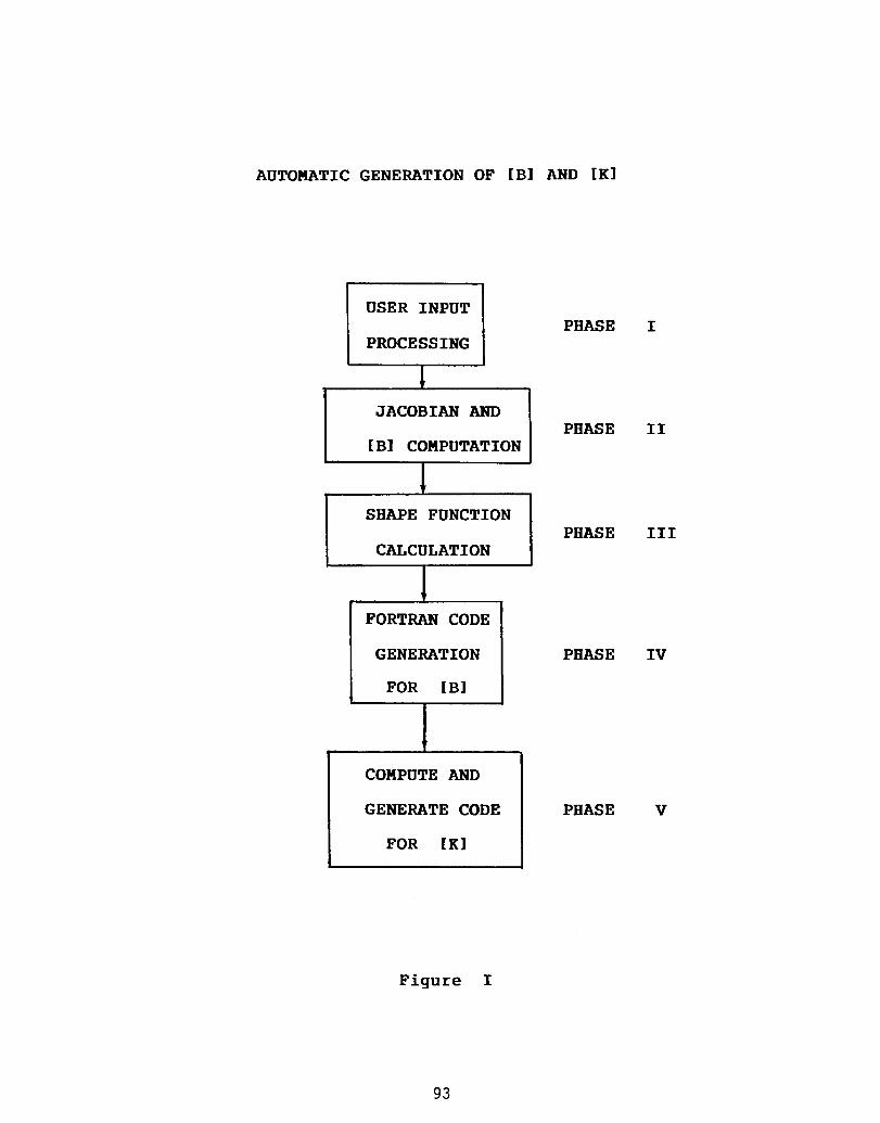
AUTOMATIC GENERATION OF [B] AND [K]
USER INPUTPHASE I
PROCESSING
JACOBIAN ANDPHASE II
[B] COMPUTATION
1SHAPE FUNCTION
PHASE IIICALCULATION
1FORTRAN CODE
GENERATION PHASE IV
FOR [B]
1COMPUTE AND
GENERATE CODE PHASE V
FOR [K]
Figure I
93
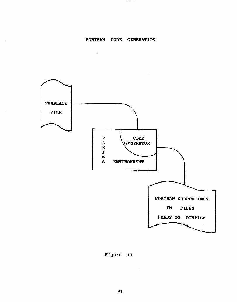
FORTRAN CODE GENERATION
TEMPLATE
FILE
V _ CODE [
xIMA E
FORTRAN SUBROUTINES
IN FILES
READY TO COMPILE
Figure II
94

STABILITY AND CONVERGENCE OF UNDERINTEGRATED
FINITE ELEMENT APPROXIMATIONS*
J. Tinsley OdenThe University of Texas
SUMMARY
An analysis of the effects of underintegration on the numerical stability and
convergence characteristics of certain classes of finite element approximations is
given. Particular attention is given to so-called hourglassing instabilities thatarise from underintegrating the stiffness matrix entries and checkerboard-instabili.-
ties that arise from underintegrating constraint terms such as those arising from
incompressibility conditions. A fundamental result reported here is the proof that
the fully integrated stiffness can be restored in some cases through a post-
processing operation.
INTRODUCTION
In virtually all finite element codes, numerical quadrature is used to evaluate
integrals defining various matrices in the equations governing the discrete model.In recent years, many practitioners underintegrate various entries in the stiffness,
constraint, or mass matrices so as to either reduce the computational effort required
to solve a problem or in attempts to improve convergence characteristics of certain
methods. By "underintegration" we mean the use of quadrature rules of an order lower
than that required to produce exact integrals of the polynomials appearing in variousfinite element matrices.
Unfortunately, the use of underintegration frequently leads to serious numerical
instabilities. Underintegration of the stiffness matrices, for example, may produce
spurious patterns in the displacement fields which are referred to as "hourglass,"
"chickenwire," or "keystone" modes, whereas underintegration of constraint terms such
as those arising from incompressibility conditions may lead to spurious oscillations
in stress or pressures known as "checkerboard" modes. An example of a checkerboardpattern in a stress field in a highly-deformed hyperelastic cylinder under axial com-
pression, computed using eight-node isoparametric elements and reduced integration of
an incompressibility constraint, is shown in Fig. i. The hourglass-instability phe-
nomene has been discussed by Flannagan and Belytschko (ref. i) in recent times, where-
as instabilities due to underintegration of penalized constraints have been studied by
Oden, Kikuchi, and Song (ref. 2), Oden and Kikuchi (ref. 3), and Oden and Jacquotte(refs. 3 and 4).
In the present paper, particular attention is given to the issue of hourglass in-stabilities in the well-known four-node isoparametric element.
This work was supported by NASA Lewis Research Center under Grant NAG3-329.
95

CObIPRFS8.I ON OF R CTL I NDER _ 88N
CONIOUR SIGMA1LORD STEP i
LOAD i:iqClOR O, 2000
Figure i. Computed stress profiles in a compressed incompressible hyperelastic cylinder showing actualspurious checkerboard modes.

STUDY OF A MODEL PROBLEM
To focus on some key features of hourglass instabilities, it suffices to consider
a model boundary-value problem defined as follows:
Find a function u _ HI(_) such that (1)7a(u,v) = (f,v) for all v in HI(_)
where
a(u,v) == I.j Vu"fv Vv dxdy 1
(2)
(f,v) I dxdy
Here _ is a smooth bounded domain in the x,y-plane, f is a smooth function de-
fined on _, a(',') is a continuous bilinear form defined on the _sual space HI(_)of functions with L2-first derivatives, and (',') denotes the L -inner product.
For simplicity, _ will generally be taken as rectangular. Problem (i), of course,is a variational statement of the Neumann problem,
I
_u-Au = f in _j _-_ = 0 on _
We next construct a standard, conforming, finite element approximation of (i) on
a uniform mesh of Ql-elements-(four node elements with bilinear shape functions),the length of the sides of each element being h . The approximate problem is then
Find uh € HhC HI(_) such that
a(uh, Vh) = (f,vh) for all vh in Hh _ (3)
where
Hh = {vh € C0(_)[Vhl _ € Ql(_e )} (4)e
To evaluate a(uh,v h) in (3), we use a Gaussian quadrature rule of the type,
E G
($.) (5)a(uh,Vh) = _ e e ee=l j=l 3 n ~3 n ~j
where
E = the total number of elements in the mesh
G = the number of Gauss points (G > 4)
97
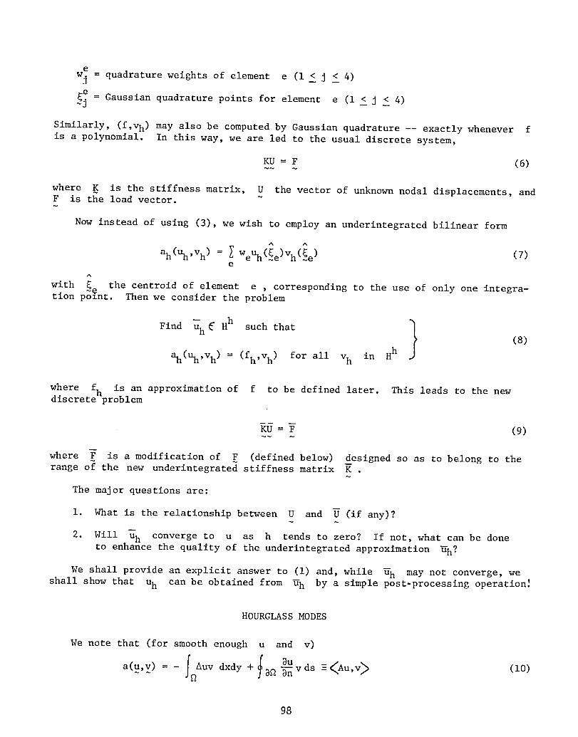
e
w. = quadrature weights of element e (i < j < 4)
e
_j = Gaussian quadrature points for element e (1 _ j _ 4)
Similarly, (f,v h) may also be computed by Gaussian quadrature -- exactly whenever fis a polynomial. In this way, we are led to the usual discrete system,
KU = F (6)
where K is the stiffness matrix, U the vector of unknown nodal displacements, andF is the load vector. ~
Now instead of using (3), we wish to employ an underintegrated bilinear form
A A
ah (Uh,Vh) = _ WeU h(_e)vh(_e ) (7)e
A
with __ the centroid of element e , corresponding to the use of only one integra-tion polnt. Then we consider the problem
Find U--h_ Hh such that 1 (g)ah(Uh,V h) = (fh,Vh) for all vh in Hh
where fh is an approximation of f to be defined later. This leads to the newdiscrete problem
KU = F (9)
where F is a modification of F (defined below) designed so as to belong to therange of the new underintegrated stiffness matrix K .
The major questions are:
i. What is the relationship between U and U (if any)?
2. Will _h converge to u as h tends to zero? If not, what can be done
to enhance the quality of the underintegrated approximation _h ?
We shall provide an explicit answer to (i) and, while u--h may not converge, weshall show that uh can be obtained from _h by a simple post-processing operation_
HOURGLASS MODES
We note that (for smooth enough u and v)
f uvdxdy + J _u <Au,v> (i0)a(u,v) =-
~ ~ _ _ _nnvds -
98
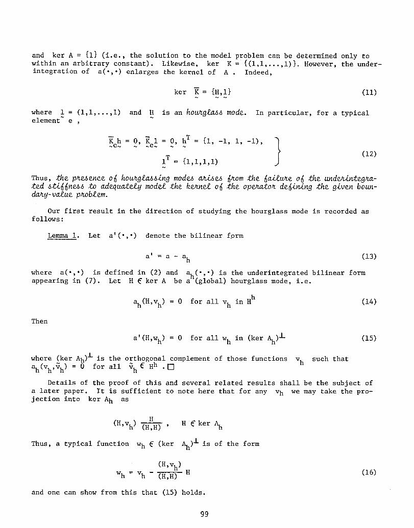
and ker A = {i} (i.e., the solution to the model problem can be determined only to
within an arbitrary constant). Likewise, ker K = {(i,i .... ,i)}. However, the under-
integration of a(.,.) enlarges the kernel of A . Indeed,
ker K = {H,I} (ii)
where 1 = (I,i,...,i) and H is an houy_g_s mode. In particular, for a typicalelement e ,
~e~h = 0,~K~e~l= ~0'hT~ = {i, -i, i, -I),
1T = {i,i,i,i) _ (12)~
Thus, the presence of hou_glassing modes arises from the f_e of the undgrZntegra-ted stiffness to adequately model the kernel of the operator defining the given boun-dary- value p_blem.
Our first result in the direction of studying the hourglass mode is recorded asfollows :
Lemma i. Let a'(',') denote the bilinear form
a' = a - ah (13)
where a(-,') is defined in (2) and a_(.,.) is the underintegrated bilinear formappearing in (7). Let H € ker A be a"(global) hourglass mode, i.e.
ah(H,v h) = 0 for all vh in Hh (14)
Then
= 0 for all wh in (ker _)J- (15)a' (H,wh)
where (ker Ah )i is the orthogonal complement of those functions vh such that
ah(Vh,V h) = 0 for all Vh _ Hh .[7
Details of the proof of this and several related results shall be the subject of
a later paper. It is sufficient to note here that for any vh we may take the pro-
jection into ker Ah as
H
(H'Vh) (H,H) ' H € ker
Thus, a typical function wh _ (ker Ah)l is of the form
(H,vh)-- H (16)
Wh = Vh (H,H)
and one can show from this that (15) holds.
99

It is clear from (16) that every vh _ Hh is of the form
vh = wh + %H , wh _ (ker _).h, % _IR
Hence,
a(uh,Vh) = ah(Uh,Wh) + Xa'(Uh,H)
= %(f,H) + (f,wh)
so that
a'(Uh,H ) = (f,H) H = hourglass mode (17)
a (Uh,W h) = (f,wh) for all wh _ (ker Ah) (18)
Since wh can be given by (16),
(f,wh) = (f (f,H) H,(H,H) Vh)
and, therefore,
(f,H) (H,Vh)ah(_,v h) = (f,vh) -
for all vh € Hh (19)
Hence, in (8) we take as fh the projection,
fh f (f,H) H (20)= - (H,H)
From (18), we have
ah(Uh,Wh) = (f,wh) - a' (Uh,Wh)
ah(Uh,Vh ) = (fh,Vh) - a' (Uh,Wh)
= ah(Uh,V h) - a'(uh,Wh)
Thus,
i00

ah(Uh-%,Vh) = -a'(uh,Wh)
(vh ,H)' a' (Uh,H) (21)= -a (Uh,Vh) + (H,H)
This result seems to implv that u and _ do not diffe_ by an how_gfx_sin_" -h hmode, else the right hand side of (21) would be zero. Thus, the procedures usually
used to correct underintegrated solutions (by adding multiples of H) may not improve
solutions. This issue is currently being explored and requires much further study.
CALCULATION OF STIFFNESS MATRICES
Confining our attention to a unit Q1 element, we introduce the matrices
T s,Ts = {1,-1,-1,1} , ~ = {i,i,-1,-1}
h T = {1,-1,1,-1} , 1T = {1,1,1,1}
= 2 3 4 T = {yl 2xT {xl,x ,x ,x } , y ,Y ,y3,y4} (22)
_{Y2-Y4, Y3-Yl, Y4-Y2, Yl-Y3 }
b2= 1_{x4-x I, Xl-X 3, x2-x 4, x3-x I}
where x.,y. = coordinates of node i, i = 1,2,3,4. We no longer confine ourselves
to a uni_or_ rectangular mesh. If (_,_) denote coordinates of a unit master QI-
element, then the stiffness matrix Ke of a typical finite element can be shown tobe given by
[ Axx TAT Ayy TA~~~~T
Kwe = f_\ yTAx + yTAx~ ~~ ]d_dn (23)
(_ = unit square)
A = -_ksl",s_T _ ss'T) + -_2(shT~~ -hTs)~~ 4- --_(hs 'T- s'hT)~~ (24)
whereas the underintegrated (one-point) stiffness matrix is
1 (blb 1 + b2b2) (25)
I01

and I_ I denotes the area of the element. The rank deficiency of K(1) follows im-mediately from the fact that ~e
bTh = 0 bTl = 0 i = 1,2 (26)
O_ goal here is to compute exa_y K {or K^) from K(I) (or K (I)) by asimple post-proc_sing operation. That this is possible foll_ws from th_ fact that
hTK h = 16 _ (27)~ ~e~
= K(1) + _yyr_e ~e ~~ (28)
where
y = h i (hTxbl-hTyb2)~~ ~ ~~ (29)
~ ~ I_e I
T 2
-- i I (_ s x- Bs'Tx) + (_(sTy -B(s'Ty)) 2= ~ ....... d_dB (30)
g _ _ If_ I+e $_Ao+ _qBo
and
A = (y4-Y3) + (yl-Y2)o (Xl-X2) (x3-x4)
Bo = (y3-Y2) (Xl-X 4) + (yl-Y4) (x2-x 3)
Note that for parallelograms, _ = [(xq-x_) 2 + (x2-x4)2 + (yl-Y3)2 + (y2-Y4)2]/24[_e l
whereas for rectangular elements of digme[er he , _ = he/iml_el.
The difference matrix,
KI = K - K(I) (31)~e ~e ~e
can be written
KI i hhre = 3 [lh][2 (32)
It 11
Upon assembly, we obtain systems
102

KU = F, K(1)U = F (33)
= F - FT_ (34)
in analogy with (3) and (8), respectively. In analogy with (21),
= i Ue(hTHH- he/llHiI (35)K [.... )e
where u = h_U/i)heilm,, ,, and ^H= H/IIHB[. We can use this result to show that~e ~e ''~ ~ ~ ~ ~
IIK(1)(U-_)li < [IK'uB] (36)
Thus, the success of the underintegration method will again depend upon how small one
can make the norm IOK'uII. This issue is to be the subject of a forthcoming paper.
CONCLUSIONS
i) The fully integrated and underintegrated finite element approximations ap-
parently do not differ by an hourglassing mode. Thus, the introducing of orthogonal
hourglassing corrections may not be sufficient to produce acceptable solutions from
underintegrated solutions. This subject requires further study.
2) On the other hand, it is possible to generate exactly the fully integrated
stiffness matrix from the underintegrated stiffness matrix using fairly simple post-
processing operations. An exact formula for such calculations has been presented in
equation (30).
REFERENCES
i. Flannagan, D.P. and Belytschko, T., "A Uniform Strain Hexahedron and Quadrila-
teral with Orthogonal Hourglass Control," InternationalJournal of Numerical
Methods in Engineering, Vol. 17, 1981, 679-706.
2. Oden, J.T., Kikuchi, N., and Song, Y.J., "Penalty-Finite Element Methods for the
Analysis of Stokesian Flows," Computer Methods in Applied Mechanics and Engin-
eering, Vol. 31, 1982, 297-329.
3. Oden, J.T. and Kikuchi, N., "Finite Element Methods for Constrained Problems in
Elasticity," International Journal of Numerical Methods in Engineering, Vol. 18,1982, 701-725.
4. Oden, J.T. and Jacquotte, O., "Stable Second-Order Accurate FiNite Element Scheme
for the Analysis of the Two-Dimensional Incompressible Viscous Flows," FiniteElements in Fluids, Vol. V, edited by J.T. Oden et al., John Wiley & Sons, Ltd.,
London (to appear).
5. Oden, J.T. and Jacquotte, 0., "Stability of Some RIP Finite Element Methods for
Stokesian Flows," TICOM Report 82-8, Austin, 1982.
103

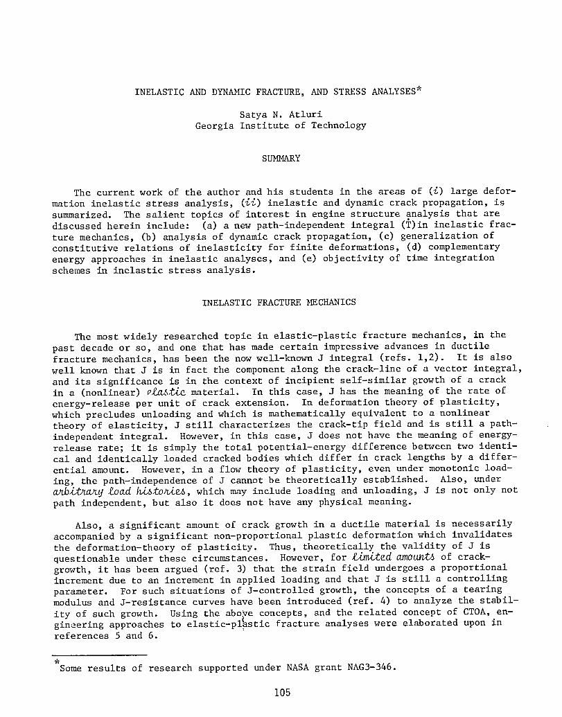
INELASTIC AND DYNAMIC FRACTURE, AND STRESS ANALYSES*
Satya N. Atluri
Georgia Institute of Technology
SUMMARY
The current work of the author and his students in the areas of (i) large defor-
mation inelastic stress analysis, (_) inelastic and dynamic crack propagation, is
summarized. The salient topics of interest in engine structure analysis that arediscussed herein include: (a) a new path-independent integral (T)in inelastic frac-
ture mechanics, (b) analysis of dynamic crack propagation, (c) generalization ofconstitutive relations of inelasticity for finite deformations, (d) complementary
energy approaches in inelastic analyses, and (e) objectivity of time integration
schemes in inelastic stress analysis.
INELASTIC FRACTURE MECHANICS
The most widely researched topic in elastic-plastic fracture mechanics, in the
past decade or so, and one that has made certain impressive advances in ductile
fracture mechanics, has been the now well-known J integral (refs. 1,2). It is also
well known that J is in fact the component along the crack-line of a vector integral,
and its significance is in the context of incipient self-similar growth of a crackin a (nonlinear) _ic material. In this case, J has the meaning of the rate of
energy-release per unit of crack extension. In deformation theory of plasticity,
which precludes unloading and which is mathematically equivalent to a nonlinear
theory of elasticity, J still characterizes the crack-tip field and is still a path-
independent integral. However, in this case, J does not have the meaning of energy-release rate; it is simply the total potential-energy difference between two identi-
cal and identically loaded cracked bodies which differ in crack lengths by a differ-ential amount. However, in a flow theory of plasticity, even under monotonic load-
ing, the path-independence of J cannot be theoretically established. Also, under
_b_y load _i_, which may include loading and unloading, J is not only not
path independent, but also it does not have any physical meaning.
Also, a significant amount of crack growth in a ductile material is necessarily
accompanied by a significant non-proportional plastic deformation which invalidates
the deformation-theory of plasticity. Thus, theoretically the validity of J is
questionable under these circumstances. However, for _ed _ou_ of crack-
growth, it has been argued (ref. 3) that the strain field undergoes a proportionalincrement due to an increment in applied loading and that J is still a controlling
parameter. For such situations of J-controlled growth, the concepts of a tearingmodulus and J-resistance curves have been introduced (ref. 4) to analyze the stabil-
ity of such growth. Using the aboye concepts, and the related concept of CTOA, en-
gineering approaches to elastic-pl_stic fracture analyses were elaborated upon inreferences 5 and 6.
Some results of research supported under NASA grant NAG3-346.
105

Thus, further research is necessary to understand the mechanics of growth initi-
ation of cracks in elastic-plastic materials subject to arbitrary loading/unloading
histories. Also, more-theoretically-valid parameters/criteria are necessary to ana-
lyze situations wherein there may be substantial amounts of stable crack-growthwhich are no longer within the limits of J-controlled growth.
Turning to the problem of crack growth in structures operating at elevated tem-
peratures --the so-called problem of creep crack-growth, numerous experiments have
recently been undertaken (refs. 7,8 for example) with the purpose of finding a pa-rameter which may correlate with the creep crack-propagation rate. Most of these
investigators considered as candidate parameters, KI, some form of net sectionstress, or in more recent studies, C*. The parameter C* has been introduced in
reference 9 and is valid only in pure steady-state creep (_ ~ an). This situation
is characterized by: (i) the body being essentially at steady-state creep condi-tions which implies very slow crack propagation and (i_) the creep-damage process
zone being local to and therefore controlled by the crack-tip field. However, sup-
pose a particular material and geometry result in a crack-propagation rate such that
elastic strains are not negligible compared to creep rates (ie., non-steady creep)
and that at the same time, creep strains are no longer localized to the crack-tipregion. While C* is not a valid parameter for this case, it appears reasonable to
expect that crack growth rate is still determined by the local crack-tip field since
the creep damage process zone is still assumed to be local to the crack-tip. Fur-
ther, even though C* is a path-independent integral at steady-state creep condi-tions, it does not seem to have any physical meaning even under such conditions.
These and other difficulties with C* have been noted in recent literature (refs. 7,8). Thus, there is a need to explore alternatives to C* which remain valid even
under non-steady creep conditions, which are path-independent integrals and which
have a well-defined physical meaning so that they may be measured in laboratoryspecimens in an unambiguous manner.
With the above objectives, the author has studied (ref. i0) certain path-inde-pendent integrals, of relevance in the presence of cracks, in nonlinear elastic and
inelastic solids. The hypothesized material properties included: (_) finite and
infinitesimal elasticity, (ii) rate-independent incremental flow theory of plastic-
ity, and (ill) rate-sensitive behavior including viscoplasticity and creep. In each
case, finite deformations were considered, along with the effects of body forces,material acceleration, and arbitrary traction!displacement conditions on the crack
front. Also, the physical interpretations of each of the integrals either in termsof crack-tip energy release rates or simply the energy-rate differences in two com-
parison cracked bodies were explored. Several differences between the presentlyobtained results and those considered well established in literature were pointedout and discussed.
We omit the mathematical details of the development but present here the end re-
sults for incremental, path-independent, vector integrals which are of relevance in
ductile fracture mechanics under arbitrary load histories. Further, for simplicity,we consider: (i) quasi-static crack growth initiation and stable crack growth and(i_) the deformations to be small, so that the distinctions between various stress
measures disappear. Consider a generic increment of external load (load-control)
from an initial state with stresses % and initial displacements u. Let the incre-
mental stresses be &T and the incremental displacements be Au. We consider two
paths FI and F2 surrounding the crack-tip. We allow the incremental potential AUfor AS to be an explicit function of the location of the material particle through
parameters _ (which can be i for plastic loading and 0 for elastic unloading) and
106
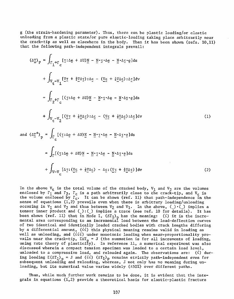
g (the strain-hardening parameter). Thus, there can be plastic loading/or elastic
unloading from a plastic state/or pure elastic-loading taking place arbitrarily nearthe crack-tlp as well as elsewhere in the body. Then it has been shown (refs. i0,ii)
that the following path-independent integrals prevail:
(&T)p =frl+rc[!:A__+ AU)N_ - _N'T'Ae~~ - N.AT.e]ds_~ ~
+_Vt_Vl[_! + ½VA_):A_ - (_ + ½VA_):A_]dv
f2+r [(/:Ae + AU)N - N-T-Ae - N.AT-e]dsc
+ _V [(V_ + ½VAT):Ag - (V_ + ½VAs):AT]dv (i)t-V2 ..........
and (&T*)p = _ [(r:ge + AU)N - N.r.Ae - N-AT.e]ds€
= _[(T:Ae + AU)N - N.T.Ae - N.A!.e]ds
+iV-V [Ar:(_V_ + ½_VA£) - A_:(VT + ½VA !)]dv (2)
In the above Vt is the total volume of the cracked body, VI and V2 are the volumes
enclosed by FI and r2, F_ is a path arbitrarily close to the crack-tip, and Vg isthe volume enclosed by Fs. It can be shown (ref. ii) that path-independence in the
sense of equations (1,2) prevails even when there is arbitrary loading/unloading
occuring in V1 and V2 and thus between V2 and VI. In the above, (~).(~) implies a
tensor inner product and (~):(~) implies a trace (see ref. i0 for details). It has
been shown (ref. ii) that in Mode I, (AT1) P has the meaning: (_) it is the incre-mental area corresponding to an incremental load between the load-deflection curves
of two identical and identically loaded cracked bodies with crack lengths differing
by a differential amount, (_) this physical meaning remains valid in loading as
well as unloading, and (_) under monotonic loading when near-proportionality pre-
vails near the crack-tip, EAT D = J (the summation is for all increments of loading,using rate theory of plasticihy). In reference ii, a numerical experiment was alsodiscussed wherein a compact tension specimen was loaded to a certain load level,
unloaded to a compressive load, and reloaded again. The observations are: (_) dur-
ing loading E(ATI) m = J and (_) (ATI) p remains strictly path-independent even forsubsequent unloading and reloading, whereas, J not only has no meaning during un-
loading, but its numerical value varies widely (±50%) over different paths.
Thus, while much further work remains to be done, it is evident that the inte-
grals in equations (1,2) provide a theoretical basis for elastic-plastic fracture
107

mechanics under arbitrary loading and when the material behavior is characterized by
realistic rate theories as opposed to a simple deformation theory. Analogous deri-
vations of path-independent incremental vector integral (AT) c valid in gen_ _-
steady creep, and a discussion of its merits as compared to the C* integral, havebeen presented elaborately by Stonesifer and Atluri (refs. 12-14).
DYNAMIC FRACTURE MECHANICS
We first consider linear elastodynamic crack propagation in a self-similar fash-
ion. Consider, for instance, a two-dimensional problem. Let the velocity of crack
propagation be denoted by the vector C, with modulus C. Consider a small loop rs,of radius _, centered around the crack-tip at time t, and assume that the crack-tip
moves by an amount (dt__C)into F_ at time t+dt, ie., s > Cdt without loss of general-
ity. Let the unit outward normal to r_ be N, and let the kinetic energy density beT(= ½pv.v, where v is the absolute velocity of a material particle and p the mass
density)] Note that v is singular near the propagating crack-tip. From studies in
reference i0, it is seen that the rate of energy release rate G per unit of elasto-
dynamic crack growth is given by:
G = (l/C) Lt C F [(W+T)N - _.e]dP = (I/C)C'G (3)
Now we consider the problem of analyzing crack-propagation in an arbitrary body,
the shape of which and the loading on which, we suppose, preclude any possibility of
an analytical solution. Suppose that we have to use a numerical solution. Such a
numerical solution may be based on a "propagating singular element" within which the
asymptotic mixed mode solution is embedded; and hence the K-factors can be evaluated
directly, as demonstrated by the author's group (refs. 15-18). However, in order to
use a simple numerical procedure, say using distorted (singular) isoparametric fi-
nite elements or non-singular isoparametric elements, it is convenient to have
available path-independent integrals which have the same meaning as the energy re-
lease rate G of equation (3). If so, the integral can be evaluated on a path that
is far removed from the crack-tip and hence is insensitive to the details of model-ing of crack-tip stress-strain fields.
Such a path-independent integral has been derived based on general conservation
laws, as shown in references i0 and 19, and is given below:
_' = fF[(W+T)N- _-e]dF +__ v [p(a-F)-e - _T]dv
+fF [(W+-W-)_+ + (r+-r-)_+ - _-e]dF = G (4)c
where (+) and (-) refer, arbitrarily, to the "upper" and "lower" crack faces; N+ =
-N- is the unit normal to Fc+; and _ are prescribed tractions on the crack fa_e.
108

The practical application of the above new path-independent integral has beendemonstrated in references 20 and 21.
GENERALIZATION OF CONSTITUTIVE RELATIONS
TO FINITE DEFORMATIONS
At a symposium on finite strain plasticity held at Stanford University in 1981,
Nagtegaal and de Jong (ref. 22) presented some interesting results for stresses
generated by simple shear of elastic-plastic and rigid-plastic materials which ex-
hibit anisotropic hardening. In the equation for the rate of change of the shift
tensor _, they used the Zaremba-Jaumann-Noll rigid body rate of _. They found the
rather spurious result that the shear stress is oscillatory in time.
The above 'anamoly' has prompted a series of investigations by Lee and hisassociates (refs. 23,24). As a 'remedy', Lee et al. (refs. 23,24) suggest the use
of a 'modified' Jaumann derivative of _ in the evolution equation for _. While theuse of such a modified derivative in the specific problem of simple shear has been
illustrated in references 23 and 24, its generalization to three-dimensional, non-
homogeneous cases is not yet fully developed. It has been suggested in reference
23 that "a complete investigation of the micro-mechanics and the structures of poss-
ible macroscopic constitutive relations will no doubt be needed to fully understand
this phenomenon and to generate a fully-tested theory".
Recently the author has shown (ref. 25) that the anamolies as described above
are not peculiar to the anisotropic plasticity alone; similar behaviour in finite
shear may result even in the case of hypo-elasticity and classical isotropic-harden-
ing plasticity theory. Thus, in reference 25, the central problem of 'generalizing'to the finite deformation case, of the constitutive relations of infinitesimal
strain theories of elasticity (hypoelasticity), and of classical plasticity with
isotropic or kinematic hardening was discussed in detail. It has been shown in ref-erence 25 that the current controversies surrounding the choice of stress rate in
the finite-strain generalizations of the constitutive relations and the anamolies
surrounding the kinematic hardening plasticity theory are easily resolvable.
Here we briefly illustrate the case of kinematic hardening plasticity. In this
case, considering a simple J2 theory, the current yield surface can be representedby:
2-2f = (o' - a'_:Co' - _') - o = 0 (5)
where (~)' denotes the deviator of a tensor, _ is the Kirchhoff stress tensor, and
is the back stress. The normality condition is:
P= %(_fl_o) (6)
We define, as in reference 25, generalized 'objective' rates, @* and _* of _ and
respectively, as follows:
109

_* = _0 _ .y.7(_.€ ) _ y8(a._) (7)
_nd 4" = _0 _ y7(_._) _ y8(a._ ) (8)
where _0 can be any one of the currently-used stress-rates. For instance,
60 = _m T- e-o- _-e (Oldroyd) (9)
_0 = 6TM~ + ~eT'°~+ o-e~~ (Cotter-Rivlin) (i0)
_0 = _m _ _'@ + _'_ (mixed-l) (ii)
60 _m +,e T T~ = ~ ~ "_ - _-e (mixed-2) (12)
_0 = _m + _'_ _ _'_ (Zaremba-Jaumann-Noll) (13)
In equations (7-13), e is the velocity gradient, _ the strain-rate, _ is the spin,and _m is the non-objective material rate. Since, for a classical continuum without
body couples, the material rate @m should be symmetric, the generalized stress rates
0* and _* are defined in reference 25, such that:
_7 = Y7 = Y8 if @0 is that of Zaremba-Jaumann-Noll (14)
_7 = (Y7+I) = (Y8+I) if @0 is that of Oldroyd (15)
P7 = (Y7-I) = (Y8-1) if @0 is that of Cotter-Rivlin (16)
_7 = (Y7-I) = (Y8+I) if @0 is that of mixed-i (17)
_7 = (Y8-I) = (Y7+I) if 60 is that of mixed-2 (18)
The linear kinematic hardening theory of Prager, as generalized to finite deforma-tions, states that:
., P= c_ (19)
110
where c is a constant of proportionality. It can be shown (ref. 25) that the plas-
tic strain-rate can be written, for the yield function given in equation (5), as:
P 3 ~ ~') -__ ) (20)- 2c_2 [(°'-_ :_*](@' ,
Using equations (7,8), (14-18), and (20), the material rates @m and _m can be writ-ten as:
_m~= ccP~ + m._~- e._~~ + _7(_-__~ + ~._'_) (21)
om 3_ ]~ ~') ~ ~'_
= 2_ + %(s:I)I - 2_ (c+2_)_2 [_:(o'-_ ](o'-e J
+_.o - @_ + _7(o.§ + §.o) (22)
In a finite shear problem, we may prescribe velocities:
vI = 2rex2 v2 = 0 (23)
such that the strain-rate E and the spin _ are, respectively:~
= 0 and _ = 0 (24)0 o
Lee et al. (refs. 23,24) consider the case when: (_) Y7 and Y8 are zero in equa-
tions (7) and (8); (_) _7 = 0 in equations (14,21,22) ie., they consider the casewhen @0 is the Zaremba-Jaumann-Noll rate. The obtained solutions are oscillatory in~
references (23,24). Thus, the generalization of Lee et al. (ref. 23,24) /6 _prope)_.
On the other hand, it has been shown by the author (ref. 25)that if _7 is ±i in equa-
tions (21,22), the ob._.ined sollggio_6 for s_esse6 are n0n-os_0ry. Furthermore,
it is seen that the condition _7 = ±i can be satisfied even when any one of thestress-rates as in equations (9-13) are used. The way to do this is to _e the
generalized st_ess-r_es _* and _* as in equatY_ns (7,8) and to choose ¥7 and ¥8 asin equations (14-18). ~
COMPLEMENTARY ENERGY APPROACHES IN INELASTIC ANALYSIS
Recently Reed and Atluri (refs. 26-31) presented comprehensive studies of a new
hybrid-stress finite element algorithm, suitable for analyses of large, quasistatic,
III

inelastic deformations. The algorithm is based on a new complementary energy prin-
ciple for rate type materials given earlier by Atluri (ref. 32). The principal var-iables in this formulation are the nominal stress-rate and spin, and the resulting
finite element equations are discrete versions of the equations of compatibility andangular momentum balance.
The algorithm produces true rates, time derivatives, as opposed to 'increments'.
There results a complete separation of the boundary value.problem (for stress-rate
and velocity) and the initial value problem (for total stress and deformation);
hence, their numerical treatments are essentially independent. In references 30-31,
a comprehensive discussion of the numerical treatment of the boundary value problem
and detailed examination of the initial value problem covering the topics of effi-
ciency, stability, and objectivity were presented. Several problems dealing withhomogeneous as well as inhomogeneous large deformations of inelastic materials were
solved, and the solutions discussed in detail. In the following, we present a briefoutline of the methodology.
The boundary-value problem for the rates of stress and spin is governed by avariational principle corresponding to the stationarity of the functional:
Hc(_,'t) = _v{-R([,_)- ½T:(_-_)+ _:_}dV +/S n.[.v dS (25)v
where m is the spin, and E is the rate of the first-Piola stress as referred to the
current configuration. In the above, R is the rate of complementary energy density,is the current Cauchy stress, _ are prescribed velocities at the boundary-segment
Sv of the solid, n is a unit outward normal to Sv, and V is the volume of the solid.
In equation (25), the following definitions and a priori constraints apply:
V-[ + 06 = 0 in V or t = V × i + _b (26)
n.t = T at S (27)
DR
_ - _ (28)
T= ½(t + T'_ + _ "T + iT) (29)
In the above, V is the gradient operator in the current configuration of the body,and _ are prescribed body forces; _ is a first-order (once-differentiable) stress-
function, _b is a particular solution for _; and s is the strain rate. The Euler-Lagrange equations that follow from _ = 0 are:
c
(Eq_)'T + t = "tT + T-(_4_ T) (30)
112

m
v = v at S (31)-- -- V
_Vv= (£+_)T (32)
Equation (30) is the angular momentum balance condition, equation (31) is the veloc-
ity boundary condition, and (32) is the kinematic compatibility condition for the
rate problem.
In the finite element formulation, we assume for each element:
NQi
Z = _ _iqN ; _ = isoparametric shapefunctions (33)
i=l
NW
= _ QWie N where QWi + QWI = 0 (34)i=l
NT
~_= _ QTiSN + ~_b where QT._m= _V × -Ii" and _V'tb~ =-ob_ (35)i=l
where NQ is the number of velocity parameters, NW is the number of spin parameters,
and NT is the number of stress parameters.
Use of equations (33-35)in (25) can be shown to lead (ref. 30) to the algebraic
system:
Kv* = f (36)
where v is the vector of global.nodal velocities. Solution of (36) leads to globalvelocities, from which the rate t and the spin W in each element can be computed.
We are thus led to initial value~problem to integrate v, t, and _ in time to find
the solution for displacement, total stress, and rotation at each material point.
In references (30-31) an elaborate study of various time-stepping schemes for
integration of the above initial value problem as to their efficiency, stability,
and objectivity was presented. In the following, we limit ourselves to a brief
description of an important and interesting aspect of this time integration--which
pertains to the question of maintaining "objectivity" of numerical integration.
113

OBJECTIVITY OF NUMERICAL INTEGRATION
In order to be called objective, a numerical approximation for a physical entity
must transform between two observer frames according to the same rule as the entityitself. An algorithm which produces an objective approximation will itself be call-
ed objective.
Suppose that as an objective rate one were to consider the Zaremba-Jaumann-Noll
rate, ie.,
D_
@0 =--_ + _.m _ m._ (37)~ Dt ....
Suppose also that the solution at time t = T is known, ie., o(r) = _ at t = T. If
the usual Euler integration approximation were used, ie.,
£(T+At) = O(T) + (_0 _ _._ +!._)At (38)
the result will be in error, since (I + _&t) is not an orthogonal tensor.
Recently two algorithms were presented (refs. 33-34) which preserve the stress-
integration and give a proper expression that is different from equation (38). In
reference 30, Reed and Atluri presented an approach that is slightly different from
that of references 33-34 in that numerical objectivity is treated as a general ques-
tion without specific reference to stress-integration. This approach involves the
concept of the so-called Jaumann integral (ref. 35) using which objectivity can bepreserved in any numerical integration. Here, we present the use of the Jaumann in-
tegral in stress-integration.
The Jaumann stress-integral, which can be viewed as operation inverse to the
Jaumann-differential of equation (37), can be written (ref. 30) as:
T(t) = J-I(t)Q(t)-T(T)-QT(t) +l [Jt(_)Q(t)'QT(_)'@0(_)'Q(_)'QT(t )]d_ (39)
where T is the true stress, and Q(t) is the solution of the differential equation:
_(t) = _(t)-9(t) ; Q(T) = I (40)
Now let to be the time such that
to = _ + OAt 0 < 8 < i (41)
we replace equation (40) by an approximate differential equation:
114
_(t)--ee.g(t); _0 = _(_+ OAt) (42)
and treat G0 as a constant in equation (42). The exact solution of equation (42)would be:
9e = 9(te) = (exp. _ete).l
sin_@t@ (i - cos0)ot6) 2= I + _ + _e (43)
~ we ~6 _6
where _o6 = _½98:_8 (44)
Now let 91 = Q(tl) = 9(T + At) (45)
Then, an approx2matXon to the Jaumann integral, equation (39), can be written as:
r r~T(r+ At) = J-l(tl)T"91"_'9~+ [(At)Jl(to)-Ql'-Qe'-°_'Q8"Q~ ~ ] ; 0 < e < 1 (46)
where tI = T + At. For 6 = ½ we obtain the so-called "generalized midpoint rule",which agrees with that presented earlier in reference 34. The formula of reference
33 cannot be recovered since they use a midpoint constitutive evaluation but fall
to properly rotate the resulting stress increment. The present concept of "objec-
tive integration" has the advantage that it provides a general framework for any
time-integration.
REFERENCES
I. Eshelby, J. D., "The Continuum Theory of Lattice Defects", Solid State Physics,
Vol. III, Academic Press, 1956, pp. 79-144.
2. Rice, J. R., "A Path Independent Integral and the Approximate Analysis of Strain
Concentration by Notches and Cracks", Journal of Applied Mechanics, Voi. 35, 1968,
pp. 379-386.
3. Hutchinson, J. W. and Paris, P. C., "Stability Analysis of J-Controlled Crack
Growth", Elastic-Plastic Fracture, ASTM STP 668, 1979, pp. 37-64.
4. Paris, P. C., Tada, H., Zahoor, A., and Ernst, H., "The Theory of Instability of
the Tearing Mode of Elastic-Plastic Crack Growth", Elastic-Plastic Fracture,
ASTM STP 668, 1979, pp. 5-36.
115
5. Kanninen, M. F. et al., "Development of a Plastic Fracture Methodology", EPRI
NP-1734, Project 601-1, Final Report, March 1981.
6. Kumar, V., German, M. D., and Shih, C. F., "An Engineering Approach for Elastic-
Plastic Fracture Analysis", EPRI NP-1931, Electric Power Research Institute
Report, July 1981.
7. Saxena, A., Ernst, H. A., and Landes, J. D., "Creep Crack Growth Behavior in
316 Stainless Steel at 594°C (II00=F) '', Sci. Paper No. 82-1DT-REACT-PI, Westing-house R & D Center, August 1982.
8. Elfer, N. C., "Constant Displacement Compliance and Crack Growth in PMMA", Dept.
Fracture Mechanics and Mechanical Properties, DFVLR, Cologne, April 1982.
9. Goldman, N. L. and Hutchinson, J. W., "Fully Plastic Crack Problems: The Center
Cracked Strip Under Plane Strain", Int. Jnl. Solids & Structures, Vol. ii, 1975,pp. 575-595.
i0. Atluri, S. N. "Path-Independent Integrals in Finite Elasticity and Inelasticity,
with Body Forces, Inertia, and Arbitrary Crack Face Conditions", EngineeringFracture Mechanics, Vol. 16, No. 3, 1982, pp. 341-364.
ii. Nakagaki, M. and Atluri, S. N., "Use of (!) Integral in Elastic-Plastic Fracture
Mechanics", Proceedings of Workshop on Mechanics of Damage and Fracture, StoneMountain, GA, November 1982 (In Press).
12. Stonesifer, R. B. and Atluri, S. N., "On a Study of the (A_)e and C* Integralsfor Fracture Analysis Under Non-Steady Creep", Engineering Fracture Mechanics,
Vol. 16, No. 5, 1982, pp. 625-643.
13. Stonesifer, R. B. and Atluri, S. N., "Moving Singularity Creep Crack Growth
Analysis with the (!)c and C* Integrals", Engineering Fracture Mechanics, Vol.16, No. 6, 1982, pp. 769-782.
14. Stonesifer, R. B. and Atluri, S. N., "A New Path-Independent Integral (!)c' andComputational Studies", NASA Contractor Report, NASA Lewis Research Center,March 1982.
15. Atluri, S. N., Nishioka, T., and Nakagaki, M., "Numerical Modeling of Dynamicand Nonlinear Crack Propagation in Finite Bodies by Moving Singular Elements",
Nonlinear and Dynamic Fracture Mechanics, (Eds. N. Perrone and S. N. Atluri),
ASME AMD Vol. 35, 1979, pp. 37-66.
16. Nishioka, T. and Atluri, S. N., "Numerical Modeling of Dynamic Crack Propagation
in Finite Bodies by 1_ving Singular Elements, Part I: Formulation and Part II:
Results", Journal of Applied Mechanics, Vol. 47, No. 3, 1980, pp. 570-576 andpp. 576-583.
17. Nishioka, T. and Atluri, S. N., "Numerical Analysis of Dynamic Crack Propaga-
tion: Generation and Prediction Studies", Engineering Fracture Mechanics, Vol.
16, No. 3, 1982, pp. 303-332.
18. Nishioka, T. and Atluri, S. N., "Finite Element Simulation of Fast Fracture in
Steel DCB Specimen", Engineering Fracture Mechanics, Vol. 16, No. 2, 1982, pp.157-175.
116

19. Nishioka, T. and Atluri, S. N., "Path-Independent Integrals, Energy Release
Rates, and General Solutions of Near-Tip Fields in Mixed Mode Dynamic Fracture
Mechanics", Engineering Fracture Mechanics, Vol. 17, 1983 (In Press).
20. Nishioka, T. and Atluri, S. N., "A Numerical Study of the Use of Path-lndepend-
ent Integrals in Dynamic Crack Propagation", Engineering Fracture Mechanics,
Vol. 17, 1983 (In Press).
21. Nishioka, T. and Atluri, S. N., "Dynamic Crack Propagation Analysis Using a New
Path-Independent Integral and Moving Nonsingular Isoparametric Elements", Pro-ceedings AIAA/ASME/ASCE Structures, Structural Dynamics, and Materials Conf.,
Lake Tahoe, May 1983.
22. Nagtegaal, J. C. and de Jong, J. E., "Some Aspects of Non-lsotropic Workharden-
ing in Finite Strain Plasticity", Plasticity of Metals at Finite Strain: Theory,
Experiment, and Computation, (Eds. E. H. Lee and R. L. Mallett), Dvn. Appl.
Mech., Stanford Univ. and Dept. Mech. Engg., RPI, pp. 65-102, 1982.
23. Lee, E. H. Mallett, R. L., and Wertheimer, T. B., "Stress Analysis for Anisotro-
pic Hardening in Finite Deformation Plasticity", RPI Report, Received October-November 1982.
24. Lee, E. H., "Finite Deformation Effects in Plasticity Theory", Developments in
Theoretical and Applied Mechanics, Published by the University of Alabama in
Huntsville, 1982, pp. 75-90.
25. Atluri, S. N., "On Constitutive Relations at Finite Strain: Elasto-Plasticity
with Isotropic or Kinematic Hardening!', Report GIT-CACM-SNA-83-16, Georgia Tech,
February 1983.
26. Reed, K. W. and Atluri, S. N., "Visco-Plasticity and Creep: A Finite Deforma-
tion Analysis Using Stress-Based Finite Elements", Advances in Aerospace Struc-
tures and Materials, (Eds. S. S. Wang and J. Renton), ASME AD-01, 1982, pp. 211-219.
27. Reed, K. W., Stonesifer, R. B., and Atluri, S. N., "Stress and Fracture Analyses
Under Elasto-Plastic and Creep Conditions", Proceedings S#mposium on Nonlinear
Constitutive Relations for High Temperature Applications, Univ. of Akron, Akron,
Ohio, May 1982.
28. Reed, K. W. and Atluri, S. N., "Hybrid Stess Finite Elements for Large Deforma-
tions of Inelastic Solids", Jnl. Computers and Structures (K. Washizu MemorialIssue), 1983 (In Press).
29. Reed, K. W. and Atluri, S. N., "On the Generalization of Certain Rate-Type Con-
stitutive Equations for Very Large Strains", Proceedings Int. Conf. on Consti-
tutive Laws for Engineering Materials Theory and Application (Eds. C. S. Desai
and R. H. Gallagher), 1983, pp. 71-77.
30. Reed, K. W. and Atluri, S. N., "Analysis of Large Quasistatic Deformations of
Inelastic Bodies by a New Hybrid-Stress Finite Element Algorithm", ComputerMethods in Applied Mechanics and Engineering, 1983 (In Press).
117

31. Reed, K. W. and Atluri, S. N., "Analysis of Large Quasistatic Deformations of
Inelastic Bodies by a New Hybrid-Stress Finite Element Algorithm: Applications",Computer Methods in Applied Mechanics and Engineering, 1983 (In Press).
32. Atluri, S. N., "On Some New General and Complementary Energy Theorems for the
Rate Problems of Finite Strain, Classical Elasto-Plasticity", Jnl. of StructuralMechanics, Vol. 8, No. i, 1980, pp. 61-92.
33. Hughes, T. J. R. and Winget, J., "Finite Rotation Effects in Numerical Integra-
tion of Rate Constitutive Equations Arising in Large-Deformation Analysis", Int.
Jnl. Num. Meth. in Engg., Vol. 15, 1980, pp. 1862-1867.
34. Rubinstein, R. and Atluri, S.N., "Objectivity of Incremental Constitutive Rela-
tions Over Finite Time Steps in Computational Finite Deformation Analysis",
Computer Methods in Applied Mechanics and Engineering, 1983 (In Press).
35. Goddard, J. D. and Miller, C., "An Inverse for the Jaumann Derivative and Some
Applications to the Rheology of Viscous Fluids", Rheologica Acta, Vol. 5, 1966,pp. 177-184.
118
INTERACTIVE FINITE ELEMENTS
FOR GENERAL ENGINE DYNAMICS ANALYSIS*
Maurice L. AdamsCase Western Reserve University
Joseph Podovan and Demeter G. Fertis
The University of Akron
SUMMARY
The major objective of this work has been to adapt general nonlinear finite-
element codes for the purpose of analyzing the dynamics of gas turbine engines. In
particular, this adaptation required the development of a squeeze-film damper ele-
ment software package and its implantation into a representative current generationcode. The ADINA code was selected because of our prior use of it and familiarity
with its internal structure and logic. This objective has been met and our results
indicate that such use of general purpose codes is a viable alternative to special-
ized codes for general dynamics analysis of engines.
INTRODUCTION
There is currently a considerable interest and level of activity in developing
computational schemes to predict general engine dynamic behavior. The general feel-
ing among researchers working on engine vibration problems is that various modes of
operation, such as blade-loss events, require a high level of analysis sophisticationto realistically model the engine. Proper account of system nonlinearities (parti-
cularly at the bearings, dampers and rubs) appears to be necessary if analytical
predictions are to be realistic. The approach described in this paper seeks to make
use of already proven general finite-element nonlinear time-transient computer codeswhich are available on the open market.
Present-day jet engine configurations have evolved to a substantial degree
through a trial-and-error process involving extensive testing. There are many fun-
damental dynamic phenomena which take place within these engines for which basic
description and understanding have yet to be generated. Nonetheless, they work well.
Modern aircraft engines are typical of current high-technology products in which the
recently acquired computing capabilities of today are being used to better under-
stand and improve what is already designed, built and operating.
A better understanding of the basic dynamic characteristics of existing and new
engine configurations is a prerequisite for producing acceptable engine efficiencies
on advanced configurations (i.e., smaller rotor/stator running clearances). Also,
*This work is sponsored by NASA Lewis Research Center under grant NSG-3283; NASA
Technical Monitor, C.C. Chamis.
119
a better definition of engine dynamic response would more than likely provide valu-able information and insights leading to reduced maintenance and overhaul costs on
existing configurations. Furthermore, application of advanced engine dynamic simu-lation methods could potentially provide a considerable cost reduction in the deve-
lopment of new engine configurations by eliminating some of the trial-and-error
process done with engine hardware development.
The emergence of advanced finite element codes, such as NASTRAN, NONSAP, MARC,
ADINA, ANSYS and ABAQUS and related algorithmic advances, have placed comprehensiveengine system dynamic analyses within reasonable reach. What remains to be done is
to develop new component element software to properly model engine rotor/stator
interactive components, such as the squeeze-film damper, within the algorithmic logicof already proven finite-element codes. This is the major mission of this work.
For good reasons, aircraft gas turbine engines use rolling element bearings
exclusively. This design philosophy has, until recent years, deprived engines of
beneficial damping inherent in many other types of rotating machinery where fluid-
film journal bearings are used. The implementation of squeeze-film dampers inrecent engine designs has now provided engine designers with an effective means of
vibration energy dissipation. The net result is that engines with squeeze-filmdampers are less sensitive to residual rotor imbalance and better able to control
vibration and transmitted force levels resulting from various excitation sourceswithin the engine.
The field of rotor dynamics has evolved to its present state primarily through
the solution to problems in classes of machinery older than aircraft engines. In
most other types of rotating machinery (e.g., steam turbines, centrifugal pumps and
compressors, fans, generators, motors, etc.) the rotor can be adequately modeled as
an Euler or Timoshenko beam [i]. In addition, the support structure holding each
bearing can often be adequately modeled as a separate mass-damping-stiffness path to
ground (i.e., to the inertial frame). Also, for most purposes, bearing dynamic pro-perties are characterized as stiffness and damping elements, linearized for small
vibration amplitudes about some static equilibrium state. With few exceptions (e.g.,Hibner [2]), it is this level of sophistication that has been utilized for the most
part in rotor-dynamics analyses of aircraft engines.
Present day aircraft engines are structurally far more complex than most othertypes of rotating machinery. The multi-shaft configuration, plus the fact that the
shafts are thin rotating shells, creates unique but significant complicating diffe-rences between aircraft engines and other machinery. Also, the stator structural
support at each rotor bearing represents anything but a separate mass-damper-stiff-
ness path to an inertial frame. In fact, setting the inertial frame for the engine
is not a simple matter when the full range of in-service maneuvers is realized. Dy-
namic paths between different bearings exist not only through the rotor but throughseveral other paths within the nonrotating engine structure, i.e., a "multi-level,"
"multi-branch" system. As many as eight significant "levels" have been identified.
Adams [3] demonstrated the use of a free-free modal vector space for the rotor
in the numerical integration of the motion equation with nonlinear journal bearings
and base-motion inputs. The resulting computer code (ROTNL) has been applied tolarge steam turbine blade-out unbalance, instability limit cycles and base-motion
excitation of nuclear machinery (earthquake and underwater explosive shock). This
same approach was later applied by Gallardo et al., [4] in developing the TETRA code
for double-spool shaft gas turbine engines. The approach used in references [3] and
120
[4] uses a standard code (i.e., NASTRAN) to generate the free-free undamped normal
modes and natural frequencies for rotor and stator configurations. Nonlinear forces
and connections between substructures are carried on the right hand side of the
equations of motion, and updated at each time step of the particular numerical inte-
gration scheme. In this approach, a special purpose code is used to perform the
integration of the motion equations, and handle input and output processing. Consi-
derable flexibility and continual program advancement is therefore convenient. Also,
this provides easier control of the basic mathematical model.
On the other hand, the major advantage of the approach summarized in our work is
that full advantage can be taken of the multiplicity of computational and modeling
advancements typical of the capability in current generation nonlinear general pur-pose finite-element codes. The disadvantage is that the general purpose code is more
of a "black box" than one's own special purpose code.
TIME-TRANSIENT NONLINEAR DYNAMIC ANALYSES
In recent years it has become evident that an important class of engine dynamic
phenomena can not be studied without accounting for the highly nonlinear forces pro-
duced at bearings/dampers, labyrinths and other close-running rotor/stator clearances
under large amplitude vibrations. In such cases, linear theory typically predicts
vibration amplitudes larger than the actual running clearances. Furthermore, impor-
tant vibratory phenomena, such as subharmonic resonance and motion limit cycles, are
"filtered" out of the problem with a linear model, giving grossly erroneous predic-
tions, qualitatively as well as quantitatively [3].
With few exceptions, nonlinear dynamics problems must be solved numerically as
time-transient responses, whether the sought answer is a steady-state periodic
motion or is strictly a transient phenomenon. The problem is mathematically catego-
rized as an initial value problem in which the displacements and velocities of the
complete system must all be specified at the beginning of the transient. From that
point forward in time, the equations of motion are numerically integrated (known as"marching) as far in time as one wishes to study the system motions and forces. If
the system is dynamically stable, the transient motion dies out yielding the steadystate response which in a system with a periodic force excitation will be periodic
motion. In a stable system with no time-varying force excitation, the transient will
die out as the system comes to rest at one of its stable static equilibrium positions.
If the system is unstable, the transient does not die out but continues to grow in
time unless or until some nonlinear mechanism in the system limits the motion to
what is frequently called a "limit cycle" [3].
In order to study the general dynamical characteristics of aircraft engines,
nonlinear dynamics computational schemes are required. The approach taken is to de-
velop software packages to model engine components which are not typically found ondynamical structures and therefore are not already built into existing nonlinear
finite element structural dynamics computer codes. The initial effort has concen-
trated on developing such a software package for squeeze-film bearing dampers.
121

OVERALL APPROACH-INTERACTIVE ELEMENTS
Considering the typical engine structural complexities, an improved computa-
tional approach is necessary if a proper transient/steady-state model is to be deve-
loped for gas turbine engines. In this approach, it appears that the finite-element
method is one of the attractive modeling techniques for such problems. Its inherent
capabilities include features essential to modern engines: i) automatically handlesmulti-branch, multi-level structures in a more direct and efficient manner than fle-
xibilities approaches, 2) well-suited to handle nonlinearities associated with struc-
tural kinematic and kinetic effects [7], 3) easily accommodates various types of
boundary and constraint conditions, and 4) easily accommodates material nonisotropyand nonlinearity [7,8]. A body of established and proven algorithms are available
which can handle these various important effects [7,9] as well as geometric comple-xities (e.g., beam, plate, 2-D and 3-D elements [i0].
The required features which are presently not available with general purpose
finite-element codes are provisions to handle rotor/stator interactive forces origi-nating from squeeze-film dampers, seals and rub/impact events. Presented herein are
the results of an effort to develop a squeeze-film damper computer software packagewhich can be "plugged" into existing finite-element codes. This work is detailed inreferences [5] and [6].
DEVELOPMENT AND IMPLANTATION OF SQUEEZE-FILM DAMPER ELEMENT
The basic implant approach is quite simple as shown in Figure 1. In addition
to the standard structural element input provided for the particular general purpose
code (i.e., host program) being used, an additional small block of fixed inputs isprovided for each damper in the model. In the computational stream for numerical
integration of the motion equations, the damper software routine is called at eachtime step of the marching scheme, and provides the total instantaneous interactive
force generated in the fluid film of the squeeze-film damper. This instantaneous
force is then applied to the structures as an "external" force. The damper also
provides an option to compute the instantaneous tangent stiffness and damping matri-
ces for the damper if such is needed for improvement to the numerical integration
scheme of the host program. Details of the formulation and solution technique usedin the squeeze film software package are detailed in reference [5].
To "experiment" with the damper element independent of a general purpose code,a small four degree-of-freedom host program was written which treated the rotor and
stator each as point masses with two degrees of freedom apiece, "joined" to eachother only by the squeeze-film damper (see Figure 2). Sample runs are shown inFigures 3, 4, 5 and 6.
As detailed in reference [6], the damper element was successfully "implanted"into the ADINA code and several case studies were made. These are summarized here
in Figures 7, 8 and 9 for a multi-bearing simple rotor and different types oftransient loading.
122

EXPERIMENTAL CONFIRMATION
A two-bearing two-damper test rig was designed and fabricated. The rotor con-sists of a slender constant diameter shaft with a concentrated diskmast at the
center of the bearing span (see Figure i0). Extensive testing was performed with
this set up and rotor vibrational orbits were measured using Bently proximity probes
and signal conditioning instrumentation. We are currently completing this work bymaking runs for this configuration using the ADINA program with squeeze-film soft-
ware package implanted. We anticipate completing our correlations of experimentaland computational results in the immediate future.
REFERENCES
i. Fertis, D. G.: Dynamics and Vibrations of Structures. Wiley, New York, 1973.
2. Hibner, D. H.: Dynamic Response of Viscous-Damped Multi-Shaft Jet Engines.AIAA Journal of Aircraft, Vol. 12, 1975, pp. 305-312.
3. Adams, M. L.: Nonlinear Dynamics of Flexible Multi-Bearing Rotors. Journal of
Sound and Vibration, Vol. 71(1), 1980, pp. 129-144.
4. Gallardo, V. C. et al.: Blade Loss Transient Dynamics Analysis. Volumes I, II
and III, Contractor's final reports and program documentation for the TETRA
program developed for NASA Lewis Research Center (Contract NAS3-22053)June 1981.
5. Adams, M. L.; Padovan, J.; and Fertis, D. G.: Engine Dynamic Analysis with
General Nonlinear Finite-Element Codes, Part I. Trans. ASME Journal of Engi-neering for Power, Vol. 104(3), July 1982, pp. 586-593.
6. Padovan, J.; Adams, M. L.; Fertis, D. G.: Zeid, I.; and Lam P.: Engine Dynamic
Analysis with General Nonlinear Finite Element Codes, Part 2. ASME Paper
No. 82-GT-292, 1982, 9 p.
7. Belytschko, T.: Nonlinear Analyses - Descriptions and Numerical Stability. In
Computer Programs in Shock and Vibrations, ed. W. Pilkey and B. Pilkey, Shock
and Vibration Information Center, Washington, D.C., 1975 , p. 537.
8. Zienkiewicz, O.D.: The Finite Element Method. McGraw-Hill, London, 1977.
9. Felippa, C. A.; and Park, K. C.: Direct Time Integration Methods in Nonlinear
Structural Dynamics. Presented at FENOMECH, University of Stutgart, 1978.
i0. Structural Mechanics Computer Programs. Ed. W. Pilkey, K. Saczalski andH. Schaeffer, University Press of Virginia, Charlottesville, 1975.
123

l
i _R,)_s,YR,yS
• . Bearing ( ....
D'L'_'_'DI'DC"_o''iI Damper XR'Xs'YR'Xs
Calling Mode fromOne-Time Input Element , F.E. Program
F X, Fy
_ F • a F m
'_xj' [_-_.]
Figure i Input/Output of Damper Code.
Y
/ STATOR (M2)
OIL FILM/
P, =55 Ps, "' I Ky
Figure 2 Simple 2-Mass 4-Degree of Freedom Test Model.
m
124
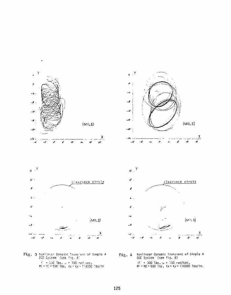
Y _.. Y . ......
0
-" -" j :",, .-::._,?..p_"- (MILS) _ , (MILS)
t
__ ..... X -a_ X
Y Y/_" - /_" .
clearance circle clearance circle
ff----_<, ff-_-..E. " "-. 8 7 "\
. _ -
0 0 - .,. --"
-4- -4.
(MILS) - (M,LS)
_. ..... _.
-,-............................. x .,_........................ x_-M -$ -_ O _ $ /_ /_" -12 -8 -_. 0 _ 8 /2 /&"
Fig. 3 boa)in..5- Dynamic Trans,er,: of Simple 4 Fig. 4 Nonlinear Dynamic Transient of Simple 4DOE System (see _g. 8" DOESystem (see Fig. 8)
'-' 'FI : 300 Ibs, _ = ;50 rad/sec,_. : 230 lbs, _ : 150 tad sec, i ,MI :_:= 500 Ibs, Kx: Ky: I_6000 ibs/i_ M1=M2:500 Ibs, Kx: Ky= 116000 Ibs/in.
125

F±g. 5 '4onl':_ '" 7L,",_mic Transien_ of Simple 4 _±g. 6 Nonlinear Dynamic Transien: of Simple 4DOEL. ._- :,_,ee Fig. 8; DOESystem {see Fig. 8)
:F I = _3_ !bs. _ = 150 rae. sec, IF t = I000 Ib$, m : 150 rad:sec,M! =;.!2:53,1 'ms, kx: Ky: _-6000 Ibsiin. Mi =M2 = 500 Ibs, Kx: Ky: :.6000 Ibs/in.
126
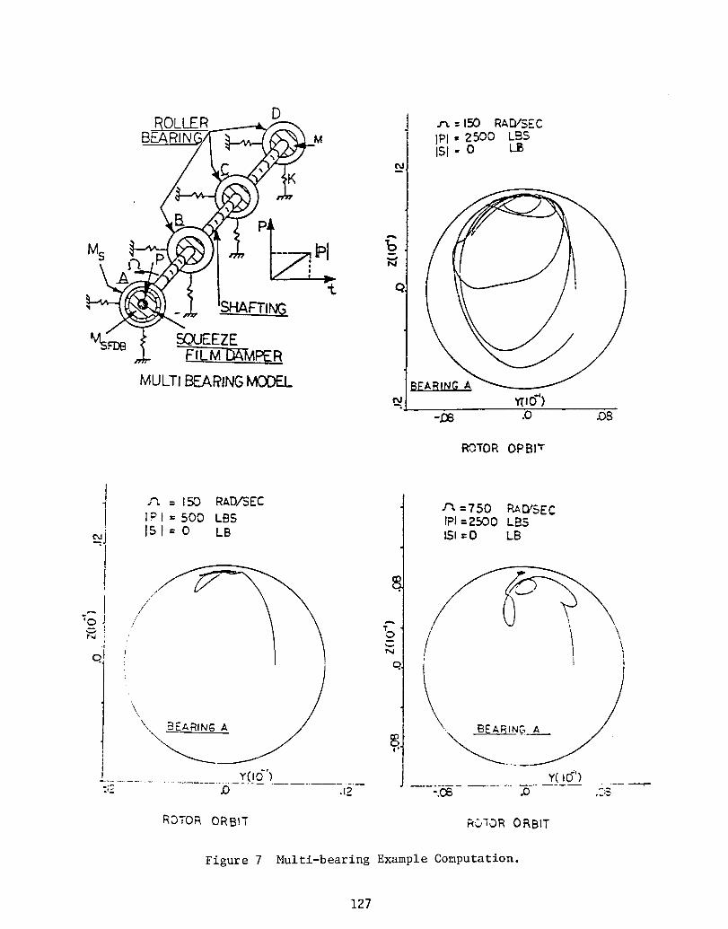
ROLLER D _ -150 RAD/SEC
BEARING//[" M IPI " 2500 LBS151" O LIBN
K
• B i P
Ms IPi g-
Ms_ SQUEEZEFiLMDA-MI_IR
MULTI BF_ARIN_SIvlC)Drr-L__ Y_O')
-DB .o OB
RO,I"OR OPBrr
I._ .m, = !50 RAD/'SEC .r_ =750 RA_SEC) I='1 : 5DO LBB IPI=2500 LB5
_j IS I = O LB ISl=O LB
"!/-
/
N 1C I ' I i
'\\.
Y(IO") Y(I_')":.i:-..................... .o...... ._2 -.c_ .o - .-_ '
ROTOROB_}_T F(C,'iORORBIT
Figure 7 Multi-bearing Example Computation.
127
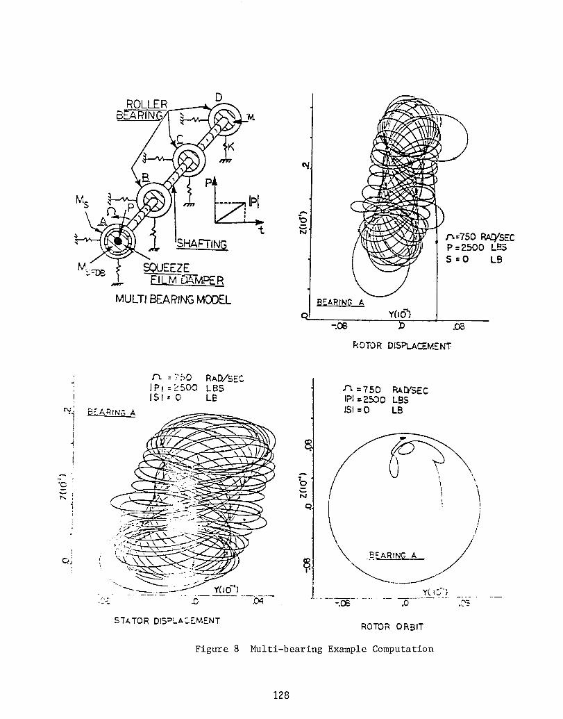
Figure 8 Multi-bearing Example Computation
128
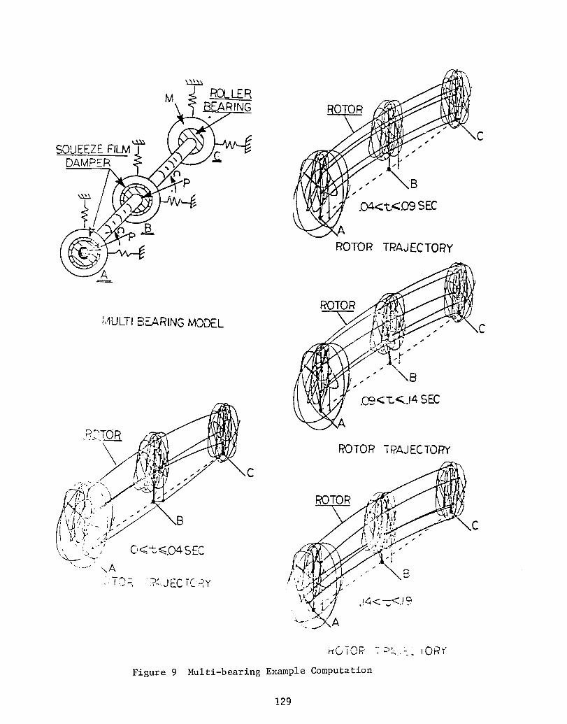
ROTORMULTI BE.ARINGMO_L
- " \CI 4
//
v
' " \B/
.09< T.,_..I4SEC
ROTOR _AJ ECTORY
C
rrOTOg ; "" " JOR'r"
Figure 9 Multi-bearing Example Computation
129

(a) Complete Test Coop With Instrumentation
(b) Rotor Test Bed With Squeeze-Film Dampers
Figure i0 Existing Experimental Test Facility Rotor
Dynamical Studies With Squeeze-Film Dampers.
130

NONLINEAR ANALYSIS FOR HIGH-TEMPERATURE
COMPOSITES - TURBINE BLADES/VANES
Dale A. Hopkins and Christos C. ChamisNASA Lewis Research Center
SUMMARY
An integratedapproachto nonlinearanalysisof high-temperaturecompositesin turbineblade/vaneapplicationsis presented. The overall strategyof thisapproach and the key elementscomprisingthis approachare summarized. Preliminaryresults for a tungsten-fiber-reinforcedsuperalloy(TFRS)compositeare discussed.
INTRODUCTION
A major thrust of currentaeropropulsionresearch is directed at improvingthe performance/efficiencyof aircraftgas turbineengines. One area of researchwhere effortshave been focusedconcernsthe potentialuse of advanced and high-temperaturecompositematerialsfor criticalengine hot-sectionapplicationssuch as high-pressureturbine (HPT)blade/vanecomponents. The temperature-limitedcapabilityof the conventionalmaterials (mostlynickel- and cobalt-based monolithicsuperalloys)used in HPT blades/vanesis a key factor affectingthe ability to augmentengineperformance/efficiency.
The ability to increasethe maximum engine operatingcycle temperatureand, thus, improveengineperformance/efficiencywould be greatly enhancedby improvingthe elevatedtemperaturecapabilityof turbineblade/vanematerials. For this reason a particularfamily of the refractory-fibermetal-matrixcategoryof high-temperaturecomposites,namely the tungsten-fiber-reinforcedsuperalloys(TFRS),are being investigated(refs.1-2) asa potentialalternativeto conventionalmonolithicsuperalloysfor use inHPT blade/vanecomponents. Moreover,a specificTFRS compositehas beenidentified(ref. 3) as having an excellentcombinationof complementarypropertiesto make it a viable candidateas a first-generationcompositeturbineblade/vanematerial.
From a qualitativeviewpoint,the potentialbenefitof using high-temperaturecompositematerials in engine hot-sectionapplications,suchas TFRS for HPT blades/vanes,is evident. Despitethe promisingoutlook,a dilemmaexists regardingthe lack of adequatemethods availabletoquantitativelyassess a high-temperaturecompositein an enginehot-sectionapplication. For example,any present attemptto analyzethe behaviorofTFRS in a HPT blade/vaneapplicationwould be forced to rely on experimentalevaluationswhich are economicallyimpractical. A definiteneed existsfor an analyticalcapabilitywith which to make a quantitativeassessmentof the mechanicalperformanceand structuralintegrityof high-temperaturecomposites,such as TFRS, in engine applications,such as HPT blades/vanes.
131

In view of the above discussion,a formalprogramwas initiatedat theNASA Lewis ResearchCenter to developa structural/stressanalysiscapabilityspecificallytailored for the nonlinearanalysisof TFRS compositeHPT blades/vanes. Although the capabilityhas been tailoredfor a specificapplication,the overallapproachof this analyticalcapabilityis generaland as such isapplicableto the analysisof practicallyany compositestructurewherematerialnonlinearityis a concern.
The emphasisthroughoutthe developmentof this structural/stressanalysiscapabilityfor TFRS compositeHPT blade/vanecomponentshas been to incorporatethe physics governingthis applicationinto the analyticalformulationof theproblem. The blade/vanecomponentsof the HPT sectionoperate in severeenvironmentswhich subjectsthem to complexand cyclic thermomechanicalloadingconditions. These loads give rise to highly nonlinearmaterial behaviorwhich,for the case of TFRS composites,is assumedto be attributableto a stress-temperature-timedependencyof the constituent(fiber/matrix/interphase)material properties. Furthermore,in the extendedserviceelevatedtemperatureenvironmentof a HPT blade/vane,TFRS compositesare subjectto a metallurgicalphenomenonknown as fiber degradationwhich involvesa chemicalinteractionat the fiber-matrixinterfaceand results in the generationof an interphaseof material.
To develop a nonlinear structural/stress analysis capability for TFRScomposite HPT blade/vane components, the COBSTRAN computer code was used asa foundation. COBSTRAN is a software package developed as an in-house researchtool at the NASA Lewis Research Center to perform linear-elastic structuralanalyses of composite blade structures. The resulting nonlinear version ofCOBSTRAN incorporates the appropriate nonlinear thermoviscoplastic (TVP)material relationships, fiber degradation expression, composite micromechanicsequations, laminate theory, and global structural analysis to relate the globalnonlinear structural response of a HPT blade/vane component to the behaviorof the TFRS composite constituent materials.
Developmentof a nonlinearversionof COBSTRANwas undertakenas anevolutionarytask. The intent is to "fine-tune"nonlinearCOBSTRANthroughan iterativeprocess of empiricalinvestigationand analyticalmethodolgyrefinement. During this iterativeprocess,nonlinearCOBSTRANwill be usedas a tool to conductparametric/sensitivitystudiesto isolatethe criticalfactorsaffectingthe behavior of TFRS compositesin HPT blade/vaneapplications.Informationfrom the parametricstudieswill be used to identifyappropriateexperimentalinvestigationsto furtherexaminethe criticalfactorsthatwarrant accountabilityin a structuralanalysis.
ANALYTICAL APPROACH
The overall approach taken here for the nonlinear structural analysis ofa TFRS composite HPT blade/vane component is illustrated in the schematic inFigure I. This schematic is representative of the general solution strategyof nonlinear COBSTRAN. This approach is referred to as an upward-integratedtop-down-structured analysis. Figure I illustrates the levels of heirarchyinvolved in this approach and summarizes the key elements comprising thisapproach.
132

The circulararrangementof Figure 1 is intendedto illustratetheincrementalnature of a nonlinearstructuralanalysisand the iterativeprocess involvedin the solutionof such a problem. The cycle correspondsto the analysisof each distinct load increment. The solutionprocess fora nonlinearanalysisby this approach involvesiterationat two levels.A primary iterationoccurs for the load incrementsof the total solutionrange. For each increment,a secondaryiterationoccurs to establishequilibrium,in the integratedsense, of the global structuralresponse.
NonlinearThermoviscoplasticRelationships
As pointed out earlier,material nonlinearityfor a TFRS compositeHPT blade/vaneis attributedto a stress-temperature-timedependencyof theconstituentmaterialproperties. To accountfor or model the materialnon-linearityin a structuralanalysis,the nonlinearTVP relationshipsshownin Figure 2 have been implementedinto nonlinearCOBSTRAN for the purposeof updating the constituentmaterial propertiesat each iterationduringthe analysissolutionprocess.
As shown in Figure 2 the nonlinearTVP expressionsprovide a relationshipbetween the currentvalue (P) and referencevalue (Po) of a materialpropertyaccordingto the currentand referencestateof the constituentmaterial asdescribedby the indicatedfield variables. The propertiesbeing modifiedinclude;normal moduli (Ell, E22), averageheat capacity (C), thermalconductivities(KII, K22), thermal expansioncoefficients(_II,_22), andremainingstrengths (SII, $22, S12).
These particularnonlinearTVP relationshipsare presentedwith therealizationthat they do not representan exact or completemathematicalmodel for describingthe nonlinearmaterialbehavior for a compositestructure.The expressionsin Figure 2 representan attemptto accountfor the materialnonlinearityinvolved in the applicationof TFRS compositesin a HPT blade/vane compenentsby treatingthe problem at the fundamentallevel.
CompositeMicromechanics
In short, compositemicromechanicsis the branch of compositemechanicswhich provides the formal structureto relate the behavior of a compositelamina to the behavior of the constituents. Compositemicromechanicsequationshave been derived to predict; the materialproperties (mechanical,thermal, anduniaxial strength)of a unidirectionalfiber-reinforcedlaminabased on thecorrespondingpropertiesof the constituentmaterials,and, the distributionof microstressesin the constituentmaterialsresultingfrom the stress stateoccurringin a lamina.
In the lamina transversedirections (2- and 3-directions,see Figure 3),the distributionof constituentmicrostresses(022, o12, 023) is non-uniformthrough the thicknessof the ply. By virtue of the nonlinearTVP relationshipsdiscussedearlier,this intralaminarnon-uniformityof transversemicrostressesresults in a non-uniformityof transversematerial propertiesfor the constituents.This intrlaminarnon-uniformityis illustratedin Figure 3 in terms of the
133

regions or zones used to characterizethe non-uniformity. Figure 3 alsolists the equationsused to calculateaverageconstituenttransverseproperties.
The compositemicromechanicsequationsfor predictinglaminamechanicalpropertiesare shown in Figure 4 togetherwith a schematicdefiningthe materialpropertycoordinateaxis system. Similarequationsexist for predictinglaminathermalpropertiesand uniaxial strengthsas well as for predictingthe distributionof constituentmicrostressesfrom the correspondinglaminastresses.
In a sense, the compositemicromechanicsequationspresentedhere canbe thoughtof as a first level of approximationfor idealizingan inhomo-geneous laminatedTFRS compositeHPT blade/vanecomponentas a pseudo-homogeneousstructure.
LaminateTheory
In short, laminatetheory (laminatedplate theory)providesthe formalstructureto describe the behavior of a laminatedcompositestructurein termsof the individuallaminaecomprisingthe laminate. A cursorysummaryof thegoverningequationsof classicallaminatedplate theory is given in Figure 5.Just as the compositemicromechanicsequationswere consideredas a first levelof approximation,laminatetheory can be thoughtof as a second level ofapproximationin idealizingan inhomogeneousTFRS compositeHPT blade/vanecomponentas a pseudo-homogeneousstructure.
Global Structural Analysis
The global finite element formulationof a general linear structuralanalysisproblem is summarizedby the equationsshown in Figure 6. Althoughthis collectionof equationspresentsa superficialview of the finite elementmethod of structuralanalysis,these equationsare representativeof thegoverningequationsof structuralanalysisas implementedin a generalpurposefinite elementcode such as NASTRAN.
The basis of the integrated approach presented here for the nonlinearanalysis of a TFRS composite HPT blade/vane component involves the applicationof the linear finite element formulation summarized in Figure 6 in an incre-mental manner.
PRELIMINARY RESULTS AND DISCUSSION
Resultswere obtainedfrom the analysisof a single unidirectionalTFRS compositelaminausing the integratedapproachjust presentedasimplementedinto nonlinearCOBSTRAN. Detailsof the analysisare leftout here as the purpose of presentingthese resultsis merely to: illus-trate the capabilitiesof this integratedanalyticalapproachby showingthe types of informationobtainable;identifytrends of material behaviorbeing accountedfor and traced in a nonlinearanalysisby this integrated
134
approach, and; point out the possible significance of a fabricationprocess in conducting a nonlinear analysis of a composite enginestructure such as a turbine blade/vane.
The results in Figure 7 were obtained from the analysis of asingle unidirectional TFRS composite lamina subjected to a temperatureload representative of the cooling portion of a typical fabricationprocess. The first plot illustrates the large longitudinal normalresidual stresses (_II) existing in the constituents at the end ofthis fabrication process. These stresses are the result of thedifference in thermal expansion coefficients between the constituents.The second plot shows the variation of longitudinal normal modulus
(Eli) for the constituents and ply during the fabrication process.Note that the modulus for the matrix initially increases but thendecreases continuously for the duration of cooling. This reflectsthe relative influence or effect of the individual dependency termsin the nonlinear TVP relationships presented earlier. At first,the temperature-dependency dominates and, as might be expected, themodulus increases to a point where the residual stress becomeslarge enough such that the stress-dependency becomes dominant. Theresults for the fiber and interphase (degraded zone) can be explainedin a similar manner. The result for the ply, as determined from thecorresponding micromechanics equation, reflects the behavior of thefiber and matrix as the volume fraction of interphase was nominal inthis case.
The third plot in Figure 7 illustrates the variation of remainingstrength available in the ply and constituents during the fabricationprocess. The results are consistent with the corresponding nonlinearTVP relationship for strength. Finally, the last plot shows the
build-up of transverse normal residual microstress (_22) in theconstituents similar to that shown for _11" The point to be notedhere is the difference in microstress fr6_ region to region for thematrix and interphase (degraded zone). This reflects the intra-laminar non-uniformity discussed earlier.
The conclusionto be drawn from these results is that perhapsthe fabricationprocess for individuallaminae,laminatepanels, anda compositecomponentitselfshould not be neglected.
REFERENCES
1. D. W. Petrasek and R. A. Signorelli, "Tungsten Fiber ReinforcedSuperalloys - A Status Review," NASA TM-82590, 1981.
2. E. A. Winsa, "Tungsten Fiber Reinforced Superalloy CompositeHigh Temperature Component Design Considerations," NASA 7%1-82811, 1982.
3. D. W. petrasek, E. A. Winsa, L. J. Westfall and R. A. Signorelli,"Tungsten Fiber Reinforced FeCrAIY - A First Generation CompositeTurbine Blade Material," NASA TM-79094, 1979.
135

SYMBOLS
k volume fraction
n, m, 1 exponential constants (equations, Figure 2)
t total time
z distance to lamina (equations, Figure 5)
A laminate membrane stiffness matrix
C heat capacity, laminate coupled membrane-bendindstiffness matrix, or global structural dampingmatrix
Cl, C2, C3 constants (equations, Figure 2)
Do, D initial fiber diameter and current fiber diameteror laminate bending stiffness matrix
E normal modulus or material property matrix
G shear modulus
K thermal conductivity or global structuralstiffness matrix
M laminate moment resultants or global structuralmass matrix
N laminate stress resultants
NT, Nm thermal and mechanical load cycles (equations, Figure 2)
Po' P initial and current value for a property (equations,Figure 2)
R lamina transformation matrix
So, S, Sc, SF initial, current remaining, cumulative, and fracturestrengths (equations, Figure 2)
To, T, Tm initial, current, and melting temperatures (equations,Figure 2)
thermal expansion coefficients
£, _o strain, and laminate midplane strains
< laminate curvatures
Poisson'sratio
136

_o, _ initial, and current stress
°o, °, _H initial, current, and reference maximum stressrates (equations, Figure 2)
vibration frequency
subscripts:
c composite or laminate
F, M, D, L fiber, matrix, interphase, and lamina
I, 2, 3 lamina material property coordinate axes
x, y, z global structural axes
137
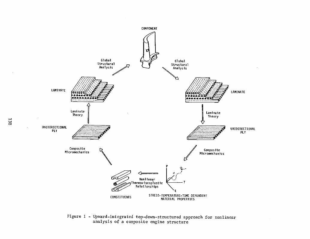
C_PONENT
Global GlobalStructural . Structural
Analyslsj
Analysis
L_INATE _ _ _ LAMINATE
Lamlnate I _ Lamlnate
_eory Theory
UNIDIRECTIONAL .._--------. _,_::::::z::::=::-
/_, ;,_._:_:___:.UNIDIRECTIONALPLY i-_::::=z:::z_::-- PLY
Composite _ / Composite
Micromechanlcs Mlcromechanlcs
P
• I,./.°o'-°Nonlinear /-_
Thermovlscoplastle _t TRelationships
CONSTITUENTS STRESS-TEMPERATURE-TIMEDEPENDENT_TERIAL PROPERTIES
Figure1 - Upward-integratedtop-down-structuredapproachfor nonlinearanalysisof a compositeenginestructure

P
--t
n m i
THERMAL PROPERTIE5 (C, K,d) P = - - 0" 6.. 5..° (Po)
REM_ININ6- STREN6TH (,S)" S = TM- C, log,oN,r- C21og,oNm-CjIog,ot (5:)- ,S,.
Figure2 - Nonlinearthermoviscoplastic(TVP)relationshipsto characterizecompositematerial nonlinearityin terms of stress-temperature-timedependentconstituentproperties
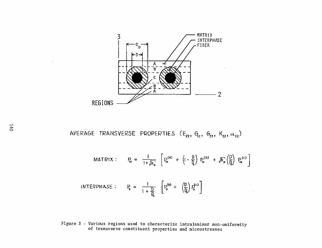
3 _ MATRIX
_ INTERPHASE
FIBER
A
A 2REGIONS
o
AVERAGE TRANSVERSE PROPERTIES (En, _2, _3, K22,°_:z)
INTERPHASE " P_- I + _
Figure3 - Variousregionsused to characterizeintralaminarnon-uniformityof transverseconstituentpropertiesandmicrostresses

Figure 4 - Composite micromechanics equations for predicting averagemechanical properties of a unidirectional fiber-reinforced ply
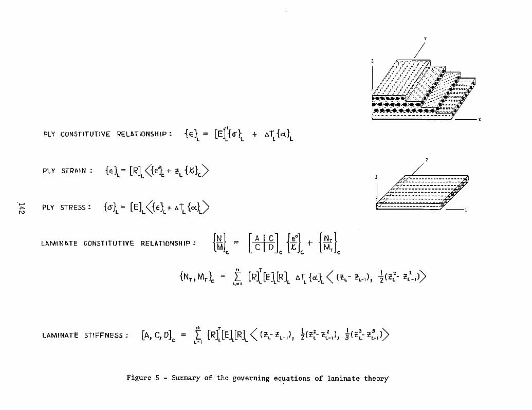
Y
/z /',','7 ',';";,'°5._
•Lo/?'/
" X
PLYCoNsr,TUTIVE REL_TiONSHIP: {e}= [E]'_{O'}L + aT{eriE
2
p._,T..,.- {o}.=[_].<{o%+_{_}_> . /3
,,_J, ................
- t []<{k r_t>-_, PLY STRESS : {_T = E e F A ct ,;_"............... . ___r_ L
{eLLAIMINhTE GONSTITUTIYE RELkTIONSfflP: M = c c
L=I
L_Iw_INATE STIFFNESS " [_# C# IZ_]G' -" _ [_]_[E]L[R]L < (EL= _ZL_,) I _C:_.L_ _:k_l)j_I 2 2 I_L_ _L_,)>::3..-3L=I
Figure 5 - Sum_nary of the governing equations of laminate theory
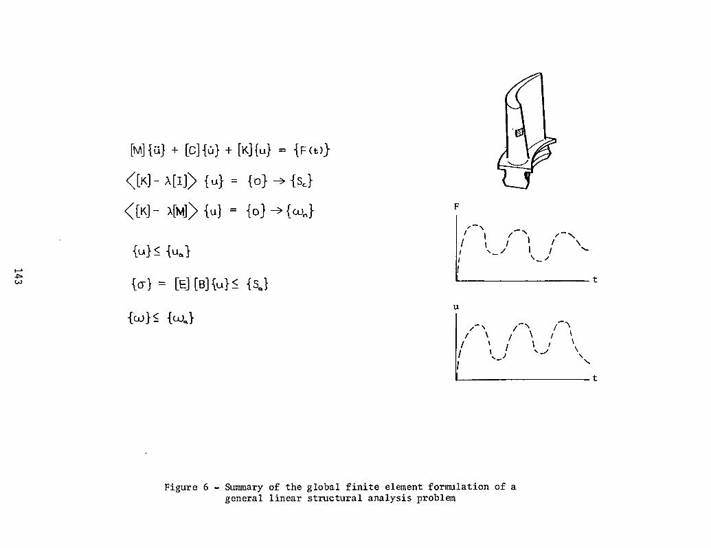
[M]{u}+ [c]{_,}+ [K]{.}= {Fc,)}
<[K]-_,[I1>{.} = {o}--->{so}
<[K]-x[M]>{,,1}: 1o}->{_o}
{-} < {'-'o'1 , , i , \•, / I I "_
{o-}= [E][_]{. }_<{sol ':U
{w}<_{,_v.}/-.,, /_._ i-A
/ \ / \ / \/ i I l I \
I I j ',-J \\I \I t
Figure6 - Summaryof theglobalfiniteelementformulationof agenerallinearstructuralanalysisproblem

F FIBERN N&TR|XO DEGRADED ZONEL PLY
HISSION LORD SPECTRUH ORRIRTION OF STRESSES2100 - flO -
II00
'10
ISOO D
20-_- Ot J il I I I I I , I I I
wry 1200 m ) I _0 O0 20000 30000 "40000 $0000
< -20
ui 900¢.5
z N -q+l)ILl I_lt--
600 -&O
-lO300
-too
o0 10000 20000 )0000 qO000 SO000 - 120
I'INE (SEC) YlNE (SEC)
Figure7 - Preliminaryresultsof an analysisof a single unidirectionallaminasubjectedto the coolinghalf of an hypotheticalfabricationprocess;variationof longitudinalnormal stress (_zt)

F FIBERH HATRIXO OEORADED ZONEL PLY
HIES/ON LOAD EPECTRUH VRRiRTION OF HECHRNICRL PROPERTIES2100 - 60
,I.SI
1000
51500 35
w 1200
1_ 2S,,€ --. L,.. 900n 20
bJ
(-_ 600 151 _K_,_,.._tA
I0 "
3006
I I I I I I I I I i
o o 1oooo 20000 )oooo _f)ooo 6o0oo o 0 1oo00 20000 30000 40oo0 Soooo
TIH£ (SEC) TIHE (SEC)
Figure 7 - continued; variation of longitudinal normal modulus (Ell)

F FIBERN NAIRIX
D DEGRADED ZONEL PLY
MISSION LO/_G SPECI.RUH V/tRI/II'ION OF STRENGTHS2100 - 3&O -
II00 320
2O01500
bJ 1200,.v 200
a¢ o.-m ,I00 .,-. 16013..,,'- _
<_ 120&O0 .
II
I I I 1 I I I I I l0 0 1oooo 20000 3111000 ,il,OOOO I0OOO 0 0 IOO00 20000 II000 40000 SHOO
IINE (SEC) lINE (SEC)
Figure7 - continued;variationof longitudinaltensilestrength (SILT)
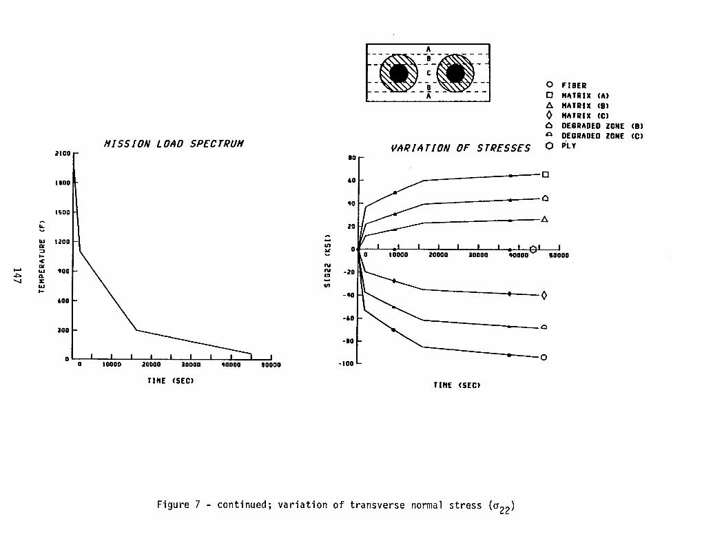
..... --m......
O FIBER
[] HATRIX (A)
A HATRIX (B)
HATRIX (C)
P' DEGRADED ZONE (B)DEGRADED ZONE (C)
HISSiON LOAD SPECTRUH VAR/AT[ON OF STRESSES 0 PLY2100 BO
• --[]
1100 601501
_ Z_zo ,.,._
1201m 1 -I I I I I I _ I ,_1 I_ 0 tO000 20000 !0000 TH)O00v SO000
_ 900 _; -20
ej_
-qO 0 --060O
-60
3OO
-00
0 _00 10000 20000 30000 '!O000 50000 -I00
;IHE (SEC) TIHE (SEC)
Figure 7 - continued; variation of transverse normal stress (_22)

THREE-DIMENSIONAL STRESS ANALYSIS USING THE BOUNDARY ELEMENT METHOD*
Raymond B. Wilson
Pratt & Whitney Aircraft
Prasanta K. Banerjee
State Universuty of New York - Buffalo
SUMMARY
The boundary element method will be extended (as part of the NASA Inelastic
Analysis Methods program) to the three-dimensional stress analysis of gas turbine
engine hot section components. This paper outlines the analytical basis of the
method (as developed in elasticity), summarizes its numerical implementation and
indicates the approaches to be followed in extending the method to includeinelastic material response.
NOTATION
V interior of three-dimensional body
S surface of three-dimensional body
ui displacement vector
eij strain tensorstress tensor
oij
ni unit normal vector
ti traction vector
fi body force distribution
Kronecker delta8ije. arbitrary unit vector
3E Young's modulus
v Poisson's ratio
shear modulus
coefficient of thermal expansion
temperature
*Work done in support of NASA contract NAS3-23697.
149
INTRODUCTION
It has been established that the durability of hot section components is amajor driver of gas turbine engine costs, in design, manufacture and maintenance.
Major savings will be realized if the lives of these components can be extended and
their cost reduced. The NASA HOST (Hot Section Structural Technology) program is
supporting a variety of approaches to these problems. As part of the HOST program aneed has been identified for an improved inelastic three-dimensional stress
analysis capability which is efficient enough for use in the design cycle. NASA
Contract NAS3-23697 (3-D Inelastic Analysis Methods for Hot Section Components),
recently awarded to the Commercial Engineering Division of Pratt & WhitneyAircraft, is directed at the development of analysis tools to meet this need.
The analysis requirements are severe. Hot section components, and the relatedstress analyses, are characterized by:
i. Extreme geometrical complexity. The components typically include surfaces
of very general shape. Small structural details must be accurately
represented, since these are frequently life limiting locations. Thecomponents usually contain holes of various sizes to allow for air and
fuel flow and these can both weaken the overall structure and act as local
stress risers. It may also be necessary to account for the presence ofsingle or multiple cracks within the structure.
2. Loading complexity. Loads typically include gas path and cooling airpressures, mechanical loads due to other components, thermal loads
(derived from unsteady temperature distributions) and, in some cases,
extremely significant centrifugal loads. Durability analysis for hot
section components requires consideration of the stress-strain history
throughout a flight cycle, and thus all of the boundary conditions andother loads are potentially time dependent. °
3. Complex material response. In all cases the elastic material response in
hot section components is inhomogeneous due to the high temperaturesinvolved and the temperature dependence of elastic modulus. In some cases
the materials are anisotropic. Inelastic response usually occurs, at least
in local regions, over some part of the flight cycle. In some cases global
inelastic response (plasticity, creep or both) of the component isencountered.
The requirements of the design process cannot readily be met using a single
analysis tool. The early phases of the design process require rapid and inexpensive
analyses of a variety of designs. In the final phase of design analysis a very
accurate determination of the stress-strain state is required for final life
prediction, but greater analysis time and cost are acceptable.
Much of the work in the present program will be devoted to the development ofsimplified (beam, shell) analysis methods for use in early design and to the
development of special purpose finite element modules for the efficient analysis ofhot section components. Significant effort will also be devoted to the extension of
the boundary element method to the three-dimensional stress analysis of hot section
components. This will provide a complementary method which can be used as an
alternative to finite element analysis. It is expected that, for some problem
classes, accuracy and efficiency will be improved relative to the use of finiteelement analysis.
150

The remainder of this paper reviews the analytical development of the elastic
boundary element method, briefly discusses its numerical implementation, gives an
example of its use for a rather complex structure and indicates the approach to be
adopted in extending the method to inelastic analysis.
ELASTIC ANALYTICAL FORMULATION
The boundary element method is a numerical method applicable to the solution
of problems in homogeneous elasticity. It is similar to the finite element methodin utilizing piecewlse approximations to geometry and field quantities. These
approximations allow the effective treatment of complex structures such as those
encountered in gas turbine engines. The boundary element method is based on anentirely different mathematical development than is the finite element method, and
this leads to profound differences in the numerical implementation. The key featureof this development is the use of classical results in mechanics and potential
theory to reduce the dlmenslonality of the problem. Thus a three-dimenslonal
elasticity problem is solved solely in terms of the surface of the body. The
mathematical development is discussed below. Further details may be found inreference i.
The starting point for the development is the Reciprocal Theorem (ref. 2)
ij elj dV = oij eij dV
v v (1)
where (°ii- li) and (o_i *, Eli) are the stresses and strains derivedfrom any _woedlsplacemen_ fields satisfying the equilibrium and compatibility
equations. Use of the strain displacement equations and the divergence theorem
allows the recasting of the Reciprocal Theorem in an alternate form involving
surface integrals of the displacement and traction fields, and volume integrals of
the displacement fields and body force distributions.
S* >* /* >*i ui dS + i ul dV = i ul dS + i ui dV (2)S V S V
The displacement states chosen are completely arbitrary, except for the
requirement that equilibrium be satisfied. For isotropic, homogeneous materials one
can identify the (*) solution with the displacement field due to a unit force• *
applled in the direction ej at the point Yi (the Kelvin solution, ref. i).Formally this is the displ_cement field satisfying
ao_j , .8x----_- = _ij 6(x,y) ej = fi (3)
151

and it can be represented in the form
* * (4)ui (x) = Gij (x,y) ej (y)
where
I [ jGij =16_ (l U)r (3 - _P) 6ij + (xi - Yi)(xj -Yj) (5)- r2
(r = Ix - Yl )
The strains, stresses and (on the surface, S) the tractions can be represented
in similar forms,
_ij = Bijk ek
* * (6)oij : Tij k ek
t_ = oij nj = Tij k nj e_ = Fik e_
where the tensors Biik, Tii k and Fik are derived from the displacement
tensor, Gij , by appr6priat_ differentiation and use of Hooke's Law. A similarapproach is available for anisotropic materials, although closed form
representations are not generally available.
By substituting u_, ti and fi in the Reciprocal Work Theoremand utilizing the formal definition of f_, an identity (Somigliana's identity)can be derived which expresses displacements at an arbitrary interior point in
terms of the displacements and tractions on the surface. Appropriatedifferentiation and use of Hooke's Law allow derivation of similar results for
stresses and strains, solely in terms of boundary data.
uj(y) = fti(x) Gij(x,y) - Fij(x,y) ui(x)] dS(x) + fi(x) Gij(x,y)dV(x) (7)S V
It then becomes possible to carry out a limiting operation in which the
interior point y approaches a specific point xo on the surface of the body. The
functions G.. and F.. both become singular, and the integral involving Fij13 1jmust be evaluated as the sum of a principal value integral and a separately
calculated jump term. After the required manipulations have been carried out, the
boundary integral (constraint) equation
[i - _ij(x)] uj(Xo) = 7[ti(x) Gij(X,Xo) - Fij(X,Xo) ui(x)] dS(x)
s (8)z"
+ 7fi(x) Gij(X,Xo) dV(x)V
152
is obtained. The tensor _ii is due to the jump term in the integral of Fij. Atany point at which the sur£ace is smooth, _ij = 1/2 _ij" At other points ztsbehavior is more complex.
The basic content of this equation is that a well posed three-dimensional
elasticity problem can be solved solely in terms of surface displacements and
tractions. The equations represent constraints on the unknown boundary data which
ensure that they will be in equilibrium with the prescribed boundary data.
ELASTIC NUMERICAL IMPLEMENTATION
While the analytical form of the boundary integral equation is of considerable
theoretical interest, there are almost no geometry and loading combinations of any
practical interest for which an exact solution exists. Classical forms of
approximation, such as series solutions, are cumbersome and, often, of questionableaccuracy. Practical exploitation of the equation thus requires a technique for
reducing it to a linear algebraic system.
Since the boundary integral equation is written in terms of the displacements
and tractions on the surface of the body, it is necessary to define a convenient
geometric approximation to the true surface and to define approximations to thedisplacement and traction variation over this surface. This allows the evaluation
of the required integrals in terms of the algebraic parameters defining thedisplacement and traction variation and, thus, reduction of the overall system to a
set of linear algebraic equations. If nonzero body forces are involved, then an
appropriate interior approximation may also be required. It need not be related to,
or consistent with the surface approximation. The solution is still carried outsolely in terms of boundary data.
Two major approaches have been taken to the three-dimensional numerical
implementation:
I. The surface is modeled as an assembly of plane triangular patches.
Displacement and traction are taken to be either constant (ref. 3) or
linearly varying (ref. 4) over each such patch. Using these approximations
it is possible to evaluate all required integrals over each surface patch
in closed form. This leads to an efficient and highly accurate calculation
of the coefficients in the resulting algebraic system. However, the
representation of complex geometry requires the use of a large number ofelements, and the limitation to linear variation of surface data tends to
reduce accuracy in cases where significant bending or large surface
element aspect ratios are involved.
2. The surface is modeled using quadratic isoparametric (fig. i) surface
patches (either quadrilateral or triangular). These are derived from the
use of similar elements in finite element analysis. Surface data is then
modeled, over each element, using the linear, quadratic or cubicisoparametric shape functions (ref. 5). Experience with this form of
representation has shown that complex geometries can be modeled using a
reasonable number of elements. The use of quadratic surface data variation
yields a significant improvement in accuracy, so that a geometrically
satisfactory model normally possesses sufficient refinement to give
sufficient definition of stresses and strains. The use of cubic variation
153
has not been found necessary in modeling gas turbine engine components.
The use of these more general approximations requires the (at least
partial) use of numerical integration in evaluating the coefficients of
the linear equation system.
Using either form of approximation, it is possible to develop algebraic
representations for interior quantities.
While both the boundary element and finite element methods are numerical
stress analysis techniques, significant differences exist between them. In
particular:
i. In the finite element method displacements are approximated throughout the
body. Stress and strain are always derived quantities. In the boundary
element method only the surface variations of both displacement and
traction are modeled. Interior results are calculated only at points where
they are desired. These interior quantities satisfy the exact equations ofelasticity.
2. A single finite element is a structure. That is, an elasticity problem can
be posed and solved for a single element. A single patch used in boundary
element method modeling is not a structure. It requires an assembly of
patches enclosing a volume before an elasticity problem can be solved.
3. The structure of a finite element system matrix and a boundary element
system matrix differ. A finite element matrix is typically large (since
the entire volume must be modeled) but is banded and symmetric. The
boundary element method matrix is significantly smaller but is typically
full (because of the surface integrals) and nonsymmetric.
TURBINE RIM COOLING HOLE
The boundary element method has been applied (using both the forms of
approximation discussed above) to the calculation of stresses.and strains at
turbine cooling hole exits, which are possible life limiting locations for turbinedisks (ref. 6). A test program was carried out, using a large scale model (fig. 2),
to determine the strain variation around the exit of a radially oriented hole
intended to feed cooling air to the blade (fig. 3). The program was designed to
study the effect of different strategies for blending the sharp corner of the holeexit.
An initial attempt was made to analyze the structure using a three-dimensional
finite element code. It did not prove possible to resolve the strain concentration
at the hole exit at a reasonable cost (for either model generation or computer
time). In order to resolve the local behavior a boundary element analysis, using
plane triangular elements (the BINTEQ code), was carried out. The quarter section
shown in figure 3 was modeled, as shown in figure 4, using 436 surface patches.Boundary conditions were taken from the finite element analysis, based on the
assumption that the overall load transfer in the finite element analysis was
correct. Results from the analysis showed good agreement with the strain gage datafrom the model tests (fig. 5).
154
The boundary element method analysis was later redone using isoparametric
elements (the BASQUE code). The model (fig. 6) required only 97 patches, areduction factor of 4.5. This reduction is directly related to the use of curved
elements, particularly in the doubly curved region at the hole exit. The results of
this analysis showed even better agreement with the data than did those of the
original analysis using plane triangles (fig. 7). The cost was significantly less,although computing system changes make an exact comparison impossible.
The results of these analyses suggest that the boundary element method is
particularly effective in resolving rapid stress and strain variations, especially
when accurate geometrical modeling is also required. This observation is consistentwith results obtained in other analyses as well (ref. 6, 7). It is not yet clear
whether the boundary element method will be competitive with finite elements for
the solution of general three-dimensional load transfer problems not involving high
gradients. In general, the methods should be viewed as complementary, not as
competitors, of which only one will eventually be used.
INHOMOGENEOUS AND INELASTIC ANALYSIS
It was noted above that the analysis of hot section components typically
involves centrifugal and nonsteady thermal loads, as well as both inhomogeneous andinelastic material response. Both the centrifugal and thermal loads can be
incorporated directly as body forces. For the centrifugal loads (where R is the
distance from the axis of rotation)
fi (_ P_2R (9)
while for the thermal loads
- _E
=_i - (i - 2 u)e'i (10)
It should be noted that these representations are not unique. The use of the
divergence theorem allows transformations of the body force terms to be carried
out. While the resulting representations are analytically equivalent the choicemade can have significant numerical effects.
The introduction of inhomogeneous and inelastic response is more complex. The
homogeneous, elastic boundary integral equation can be written, in operator
notation, as
L(v) = F (Ii)
155
where L is a linear operator, v is the unknown surface data and F is derived from
all known loads and surface data. Other linear operators exist for the calculation
of any desired interior results:
u = lu(V ) + Fu
(12)e = le(V) + Fe
O = Io(V ) + Fo
The stresses and strains obtained using the operators IE and I_ will satisfyHooke's Law using the assumed homogeneous elastic modulus. If either inhomogeneityor inelastic response occurs, then the interior stresses and strains will not
satisfy the true stress strain relation. This imbalance can be represented in termsof modified body forces and surface tractions or as volume distributions of initial
stress or initial strain. If, for example, the body force representation is chosen,
then the imbalance can be cycled back to the boundary integral equation
S V
where f_ is derived from the interior imbalance evaluation. The new boundarysolution u_, t_ will produce interior results which reduce the interiorimbalance due to the inhomogeneous and inelastic behavior. In matrix form the
system equation becomes
[T] _i + [U] t_I = £+ f__l (14)
It is particularly important to note that the kernel functions and the
matrices [T] and [U] remain unchanged during the iteration process. Thus the
calculation of these matrices and the decomposition of the system matrices need be
done only once for the entire analysis. The overall solution sequence, written inoperator form is then
calculate L 1
calculate N single elastic calculations (15)calculate L-I
calculate F
fo = 0Vi = L-I(F + fi) inelas tic/inhomogeneous time/load+i
= N (Vi) iteration stepping
t = t + At
156
The sequence presented above is valid for a single time or load increment. The
quantities u, t and F must, for an inelastic analysis, be regarded as eitherincrements or rates depending on the type of inelastic material model used. In
either case a number of time steps or load increments will be required for the
complete solution. The key point to be noted is that the surface and volume
problems have been uncoupled. In a sense the overall structural analysis problem is
solved on the surface while the complex material response is evaluated in the
interior. It remains unnecessary to have compatibility between the surface andvolume discretlzations.
Significant progress has been made in the application of these techniques in
two-dimenslonal analysis (ref. 8, 9). It is to be expected that, with careful
attention to the details of the numerical implementation, the inelastic
three-dlmensional boundary element method will prove to be highly effective formany problems of practical importance.
REFERENCES
i. Banerjee, P. K. and Butterfield, R.: Boundary Element Methods in Engineering
Science. McGraw-Hill (UK), 1981.
2. Sokolnikoff, I. S.: Mathematical Theory of Elasticity. McGraw-Hill, 1956.
3. Cruse, T. A.: Application of the Boundary Integral Equation Method to Three
Dimensional Stress Analysis. Computer and Structs, 3, 509-527 (1973).
4. Cruse, T. A.: An Improved Boundary Integral Equation Method for Three
Dimensional Elastic Stress Analysis. Computer and Structs, 4, 741-754 (1974).
5. Lachat, J. C. and Watson, J. 0.: Effective Numerical Treatment of Boundary
Integral Equations: A Formulation for Three-Dimensional Elasto-Statics. Int. J.
Num. Meth. in Engng., i0, 991-1005 (1976).
6. Wilson, R. B., Potter, R. G. and Wong, J. K.: Boundary Integral Equation
Analysis of an Advanced Turbine Disk Rim-Slot. Paper No. 14, Proc AGARD Cont.
(1978).
7. Wilson, R. B., Potter, R. G. and Cruse, T. A.: Calculations of
Three-Dimensional Concentrated Stress Fields by Boundary Integral Method.
Symposium on the Unification of Finite Elements, Finite Differences and
Boundary Integral Equations, University of Connecticut, 1978.
8. Banerjee, P. K., Cathie, D. N. and Davies, T. G.: Two and Three-Dimensional
Problems of Elasto-Plasticity. Developments in Boundary Element Methods,
Banerjee, P. K. and Butterfield, R. (ed), Applied Science Publishers, 1979.
9. Marjaria, M. and Mukherjee, S.: Improved Boundary Integral Equation Method for
Time Dependent Inelastic Deformation in Metals. Int. J. Num. Meth. in Engrg.,
15, 97-111, 1979.
157

I
7 8
Xi (_) = Ma('_)Xla a = 1,2,---,8
MI (_1 = 1/4(_'1+11 1_2+11 {_1. _2- 1)
M51_[1= 1/21_'1*1) (1- _[221
Figure i Quadratic Isoparametric Shape Functions
/- RIMSLOT-COOLINGHOLENTERSECTION
I--.-A
L-.-kSECTIONA-A
I ENGINE_ (REF.)*
Figure 2 Disk Rim Model in Test Rig Figure 3 Rim Slot-Coollng HoleIntersection
158

\
Second(blended)BIE First(unblended)DIE Finiteelementmodel
Intersectionleometrymodel intersectionI[eometrymodel Displacementsfromradialandtanlentlalloadcases
independentlyappliedto bothBIEmodels
Figure 4 Piecewise Linear Three-Dimensional Boundary Integral Equation Models for
Analysis of Turbine Disk Rim Slot-Cooling Hole Intersection
RADIAL
M_ L_AD PLANE4A
TANGENTIAL RADIALO.LOAD LOAD
TANGENTIAL ._ I I )
LOAD_ _ ,,.,.P
4.0--
O
O3.0 __
< Ou. t-
OZ <O 2.0 u. 2.0-
TEST: O I- Z< O (
BINTEQ: _ n- __I- 1.0 ,( 1.0Z
I-Z
° I "Z O
•1.0 OZ "l-
t--cn <[
I I I-r" .2.0 I0 0.5 1.0 1.5 u') 0 0.5 1.0 1.5
NONDIMENSIONAL LENGTH ALONG HOLE NONDIMENSIONAL LENGTH ALONG HOLE
Figure 5 Correlation of Test and Boundary Integral Equation Results-SecondIntersection Geometry, Planes 2A and 4A
159

MODEL USING 97 QUADRATICISOPARAMETRIC ELEMENTS
Figure 6 Quadratic Isoparametric Boundary Integral Equation Map for Analysis of
Turbine Disk Rim Slot-Cooling Hole Intersection
Plane4A
0.0
-2.0 I ; f0,5 1.0 1.5
NONDIMENSIONAL LENGTH ALONG HOLE
Figure 7 Improvement Due to Higher Order Boundary Integral Equation Modeling
160

SUMMARY
Christos C. Chamis
National Aeronauticsand Space AdministrationLewis ResearchCenterCleveland,Ohio 44135
Significantresults,conclusions,and issuesaddressedat the Lewis/Industry/UniversityWorkshopon NonlinearStructuralAnalysisare summarizedbelow by discipline: New Concepts/Formulations,Algorithms/Convergence,andInelasticAnalysis and Interactiveelements.
New concepts/formulations.- (1) The slave finite elementapproachtononlinearanalysisis viable. The large number of degreesof freedom (DOF)associatedwith this approach,however,would requireinnovativecomputationalalgorithmsto obtain computationaleffectivenesscomparedwith traditionalapproaches. The ease in changing incrementsteps, the increaseddetailedinformationavailablewithin the subinterval,and accuracydemonstratedtodate for elasticproblemsare promising. (2) A new variationalprinciplehasbeen developed. This principleis based on the combinedHellinger-Reissnerand Hu-Washizuprincipleswith additionalinternaldisplacementDOF. Hybridstress elementsbased on this new principlehave invariantpropertiesand areless sensitiveto geometricdistortions. This new variationalprincipleisconsideredto representa significantadvance in finite elementdevelopment.(3) The three-dimensionaldegeneratedelementsoffer modelingand computa-tionalefficiencyfor the analysisof generalshellswith layeredstructure,undergoinglarge deformations(in-plane,bending,and shear) and transientmotions. As expected,these elements take more computationaltime for specialshell problemscomparedwith finite elementsbased on deformableshelltheories. (4) A nine-nodeLagrangeshell finite elementproved effectiveinthe buckling,postbuckling,and elastic-plasticanalysesof shells. This ele-ment did _ot exhibit "shear locking"even in very large aspect ratio shells(up to 10_). Applicationof the elementto other nonlinearproblemssuch asdynamic, creep buckling,and ratchetingrequiresadditionalresearch. Themagnitudeof the effort requiredto developthe elementformulationfor theseother nonlinearproblemsmay be substantiallyreducedusing symboliclanguagemanipulators.
Algorithms/convergence.- (1) The new computationalalgorithmdevelopedfor self-adaptivesolutionstrategiesproved to be very effectivein the solu-tion of two highly nonlinearproblems (snap-throughload-deformationhistoryof a sphericalcap and a box-truss). This new algorithmis stable,eliminatesthe need for global inverse,and handles problemswith turningpoints andgeneralmaterial properties. Formalestablishmentof convergenceand stabil-ity characteristicsof the algorithmrequiresadditionalresearch. (2)Element-by-element(EBE) approximatefactorizationtechniqueswere comparedtotest problemsfor elasticand elastic-perfectlyplasticcantileverbeams withand without a circularhole. The EBE solutionmethod convergedwith seveniterations(with the hole) and four iterations(withoutthe hole). EBE is alinearequation-solvingprocedure. Direct use to developEBE time stepping-solution algorithmsrequiresadditonalresearch. (3) Finite elementgenera-tors using symbolicmanipulatorlanguages(VAXIMA)are viable. Initial
161
results show that the lines of program required to generate the strain-displacement and stiffness element matrices can be reduced substantially. (4)The stability convergence of underintegrated finite element approximations canbe improved by simple post-processing operations. These operations can bedescribed by an exact formula in some cases. Additional research is neededfor more general cases.
Inelastic analysis and interactive elements. - (1) Elastic-plastic frac-ture under arbitrary loading and material behavior, characterized by realisticcrack-growth rates, can be described by two integral equations. A newpath-independent integral has been derived to describe dynamic crack propaga-tion. A set of equations/conditions has been developed which generalizes theconstitutive relations for inelasticity and finite deformations. Variationalprinciples were used to derive a hybrid finite element for describing dynamiccrack propagation. (2) Interactive finite elements can be used to describethe dynamic interaction of rotating squeeze film bearings, shafts, and sup-ports. This type of analysis is the only one available to date whichdescribes the dynamic interaction in an integrated manner and which can beused as a "plug-in" in general purpose finite element codes. The interactivefinite element approach is presently being confirmed experimentally using atwo-bearing, two-damper test rig. (3) An upward-integrated and "top-downtraced" computerized capability has been developed for the nonlinear analysisof high-temperature composites applicable to turbine blades and vanes. Thistheory accounts for the complex thermoviscoplastic behavior of composites inturbine environments and includes effects of the fabrication process. Initialresults indicate that the fabrication process induces a substantial thermo-viscoplastic stress state in the composite. (4) Boundary element methods haveproven computationally effective for two-dimensional linear problems. Exten-sions to three-dimensional, nonlinear and time-dependent problems is thesubject of current focused research. It is anticipated that boundary elementswill provide a complementary analysis methodology to finite element methods.
Collectively, the summary points out the multidisciplinary approachnecessary to develop methods for complex nonlinear structural analysisproblems. This multidisciplinary approach encompasses new formulations andconcepts, invention of more general variational principles, finite elementgenerators, development of interactive elements, innovative solution algo-rithms, adaptive solution strategies, and formal criteria for a priori assess-ing solution stability and convergence. The contributors to these proceedingsdescribe what can be done, future potential, and direction in each discipline.
The goal of the highly focused research described in these proceedings isto develop methodologies which lead to designs of more cost-effective andreliable engine structures and components. It is hoped that, in addition,these proceedings will provide a valuable source of information of on-goingresearch and future direction in nonlinear structural analysis in general.
162

INDEX
Acceleration,secant,48 Composites(cont.)
Admissible,3 InhomogeneousTFRS, 134
Admissible,3 Intralaminar
Ahmad,45, 49 Microstresses,133
Algorithm, Non-uniformity,134
Hierarchial,58 Lamina,133
Hybrid-stressfiniteelement,111 Mechanicalstrength,133
IncrementalNewton-Raphson,55 Mechanics,133
Newmark,12 Micremechanics,133, 134
Newton-Raphson,46, 49 Refractory-fibermetal-matrix,131
Parabolicregularization,66, 67 Thermalstrength,133
Analysis UnidirectionalTFRS, 134, 135
Boundaryelementmethod, 154 see Tungsten-fiber-reinforcedsuperalloysGlobal 132 Computercode
Postbuckling,46 ADINA, 122
Thin plate,47 COBSTRAN,132, 133, 134Thin she11,47 FORTRAN,85, 86
Top-down-structured132 FORTRAN77, 88, 89
Upward-integrated132 Interactiveprompting, 8T
Applicationlevels,hierarchial,51 LISP,8T, 89, 90
Arc length,constrained,46, 49 MACSYMA, iii,85, 86
Aspectratio,Large,iii Menu driven, 87
Attributes, self-adaptive, 56, 51 NASTRAN,120, 121, 134TETRA, 120
Beam, cantilever,11 User-levelprograms,go
Bearingdampers,squeeze-film,121 VAXIMA,86, 87, 89
Bearings Computeroperatingsystem,UNIX, 86, 88
Fluid-filmjournal,120 Computers,VAX-II/T80,86, 91Rollingelement,120 Concaveshape,49
Behavior Configuration,multi-shaft,120
Inelastic,156 Conservationlaws, 108
Inhomogeneous,156 Constitutivelaws,3
Pre-postbuckling,60 Constitutiverelation,105
Rate sensitive,106 constraint
Bending Circular,56
Modes, inextensional,20 Hyperbolic,56
Static,35 Surfaceof, 56
Bilinear,9T Contourline, 74
Blade/vanecomponents,high-pressureturbine convergence,162
(HPT),131, 132 Criteria,iii
Boundaryelement,154, 155, 162 Rates,superlinear,56Boundaryelementmethod, 149 Stable,57
Boundaryintegral,iii convexshape,49Coordinates,curvilinear,33
Cap cowper,22
Sandwichspherical,48 Crack propagation
Spherical,36, 60 Dynamic, 105, 162Closednesscriterion,56 E1astodynamic,108
Composites Self-similar,1052, 108Constituentmaterials,132 - 134 See also creep
Fiber reinforced,31 Creep
High-temperaturematerials,131, 162 Behavior,elastic-plastic,55, 56
163
Creep (cont.) Elliptic, 56Crack-growth, 106 Energy, complementary, iii, 112Damageprocess, 106 EquationSteady-state 106 Boundary integral, 153
Cycle, limit, 121 Euler-Lagrange, 112Micromechanics, 132
Dampers, squeeze-film, 120, 122, 123 Euclidean norm, 58{)awe,22 Euler-Lagrange,112Deflection,large,48 Factorization,16
Deformation Alternatingdirectionmethod,65
Elastic-plastic,48 Element-byelement,65, 66, TO, II, 16l
Inelastic,ll2 Fractionalstepsmethod,65
Large,46, 47 Methodsof discretization,65, 66
Theoryof, 105 Splitting-upmethod,65
Determinantratio,49 Weak approximationmethod,65
Derivative Finiteelements,33, 85, 86, Ill
Spatial,3 Analysis,45, 55
Temporal,3 Conforming,approximation,97Discretizations,65 Generatorsof, 161
Non-prismatic,10 Global, 134
Semi-prismatic,10 Hybridstress,iii
Displacements Interactive,iii, 162
Constrained,48 Nonlinearsimulation,55
Internal,20 Slave,iii, 16l
Staticallycondensed,18 Flow theory,rate-independent,106Distortions,geometric,20 Forceexcitation,periodic,121Dynamics,nonlinear,121 Formulation
Galerkin,57
Eight-node,20 Rayleigh-Ritz,57
Elastic-plasticmaterial,Bilinear,4(3 Virtualwork, 57Elastic-plastic,46 Fracture
Elasticity Dynamic, iii
Finite, 106 Mechanics, 105, 107Infinitesimal, 106 Elastic-plastic, 107, 162
Element-by-element, iii Frequencies, natural, 121Elements Function,bilinear,7, 8
Bilinearquadrilateral,72 Functional,ll2Boundary,15l
Cylindrical shell, 22 Global inversion, 57Degenerated, 161 Global updating, 57Higher order, 87 Green-Lagrange, 32, 33Hybrid, II Growth,self-similar,105Hybridsemi-Loof,21
I_licit-explicit,11 Hamilton'slaw, 1, 2
Invariant,17, 20 Hardening,anisotropic,109Isoparametric,155 Heat conduction,nonlinear,56
Lagrange,46 Heirarchy,132
Nine-node,47 Hellinger-Reissner,17, 18quadralateralisoparametric,60 Higherorder,46
Semi-loof,17,20-22 Hinge,plastic,4(3
Thin shell,20, 21 Hu-Washizu,17
Three-dimensionaldegenerated,31, 32, 40 Hybridelements,17
Time-adaptivein_)licit-explicitpartition Hypo-elasticity,109of, II
Twe-dimensional,40 Incompressibility,95
164

Inelastic analysis, iii, 149 Modes (cont.)Instabilities, hourglass, 92 Free-free undampednormal, 121Instantaneous, 122 Hourglass, 95, 98, 99Integral Keystone, 95
Path-independent, 105, 106, 108, 109, 162 Rigid body, 20Principal value, 152 Morley, 22
Integration Motion, geometrically nonlinear, 32Reduced, 45 Multi-branch, multi-level system, 120, 122direct, Newmark, 35 Multi-cemponent splitting formulae
Interphase, 132, 135 Two-pass, 69, 70Invariant, 18 One-pass, 70Iron, 45, 49 Multiprocessor computer, 66Isoparametric,18Instabilities,numerical,95 NFAP,88, 91
Iteration,Newton-Raphson,48 Ne_rnark,35, 75
0 integral,105 Newton-Raphson,46
Oaumannintegral,ll5 Nonlinear,85
Jump term, 152, 153 Nonlinearity
Kinematic,55
Labyrinths, 121 Material,55
Lagrange,46 Noor, 36
Lagrangeelement Normalitycondition,109
Higherorder,47Nine-node, 48 Objectivity, 113, 105, 114
LagrangianKinematical, 75 Panel, circular cylindrical, 35Total, 32 Parallelizable, 70
Lamina transverse directions, 133 Partitions, implicit-explicit mesh, 77Laminate theory, 132, 134 Patch test, 18Large global arrays, factorizing, 65 PatchesLimit cycle, 121 Quadratic isoparametric surface, 153Load, temperature, 135 Triangular, 153Loading/unloading histories, 106 Path-independent, iii
Patterns, spurious, 95Manipulation, algebraic, 85 Phenomenon,transient, 121Marguerre, 22 Piola-Kirchoff. 32, 58Material Plastic deformation, non-proportional, 105
Elastic, 48 Plastic zone, 49Elastic-plastic, 48, 109 Plasticity theoryElastic-perfectly plastic, 48, 12, 13 Linear kinematic hardening, 110Rigid-plastic, 109 Isotropic-hardening, 109
Matrix Plates, twisted, 36Lumpedmass, 72 PolynemialsTangentdamping,77 Bilinear,18
Tangentstiffness,IT Interpolation,88Membrane Quadratic,46
Action,49 Positivedefinite,71, 17
quadrilateral, 18 Positive semi-definite, 17Stresses, momentless, 22 Postbuckling, 48, 49
Meshpartitions, implicit-explicit, 66 Algorithm, 48Micro-mechanics, 109 Analysis, artificial spring method, 46Mindlin, 46 Prebuckling, 49Modes Pre-postbuckling, elastic, 56
Checkerboard, 95 Pressure, 48Chickenwire, 95 Follower, 48
165

Pressure (cont.) Shell theoryConstant-direction, 48 Cylindrical, 22
Principle, variational, iii, 18, 161 Deep shallow, 22Prismatic, 2 Shallow, 22Propagating singular element, 108 Solid element, degenerated, 22
Solution
Quadrature Curve, 56Gaussian, 98 Self-adaptive, 161Numerical, 95 Semigliana's identity, 152
Quadrilateral planform, 21 Space-time, 3Splitting, two-cemponent, 69
Ramberg-Osgood,7 Stationarity, 112Ramm, 46, 50 Stiffness,incrementaltangent,46
Rank, 18 Strain
Rate Green-Lagrangian,33
ObJective,109, lIO MementIessmembrane,20
Strain, 111 Rate, 111
Stress, 110, 112 Stress
Zaremba-Oaumann-No11,111 Dependency,135
Rayleigh-Ritz,58 Hybrid, 19
Relations,macroscopicconstitutive,109 Incremental,33
Resonance,subharmonic,121 Largedeformationinelasticanalysis,105
Response,transient,35, 36 Tensor,Piola-Kirchhoff,32, 58
Riks, 46, 50 Stress-strainfield,Crack-tip,108
Roilingcontact,56 Stricklin,36Rotor-stator Structuralanalysis,134
As interactivecomponents,120 Structure,box truss,60
Clearances,121 SubdomainmodeI,lOInteractiveforces,122 Subgroups,Non-contiguous,70
Rub/impact,122 Substructures,lOSuperelements,70
Safetyzones,56 Sweptpanel,20
Seals,122 S_ymbolic,85, 86
Secantaccelerated,46 Expressions,89
Self-adaptive,iii Processing,87
Semi-discrete,15 TFRS, see Tungsten-fiber-reinforcedsuperalloys
SemiLoof,see Elements Tangentstiffness,singularityof, 46
Sensitivitystudies,132 Taylorseries, 58
Serendipity,46 Temperaturedependency,135
Shape function, 87 Temporal,3Shear Test rig, 123
Locking,45, 47 TheoryFinite, 111 Deformation,105
Shell Four-dimensionalunified, 10
Angle-ply,36, 40 Laminate,132
Cross-ply,36, 40 Thermoviscoplastic(TVP),nonlinear,iii, 132,Cylindrical,36, 40 133, 135Degenerated,45, 47 Thinplate analysis,47
Elements,47 Thin shellanalysis,47
Laminatedanisotropic,31 Top-downtraced,162
Largeaspect ratio,161 Transient,geometricallynonlinear,31Shear-deformed,iii Triangularelements,21, 22
Spherical,36 Tungsten-fiber-reinforcedsuperalloys(TFRS),Sphericalshallow,48 131,132, 134
Theory,22 Blades/vanes,133
Thin rotating,120 Fiber degradationof, 132
166
Tungsten-fiber-reinforced superalloys (cont.) Vibration, natural, 35, 36Fiber-matrix interface of, 132 Viscoplasticity, 106Nonlinear analysis of, 132
Turningpoints, 56 Work theorem, reciprocal, 152
Underintegration, 95 Zienkiewicz, 45, 49Bilinear, 9B Zone, degraded, 135
Unstable, 48Upward-integrated, 162
167
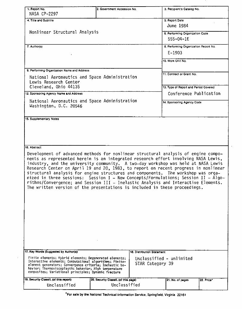
1. Report No. 2. Government Accession No. 3. Recipient's Catalog No.
NASACP-2297
4. Title and Subtitle 5. Report Date
June 1984
Nonlinear Structural Analysis 6 Performing Organization Code
555-04-IE
7. Author(s) 8. Performing Organization Report No.
E-1903
10. Work Unit No.
9. Performing Organization Name and Address11. Contract or Grant No.
National Aeronautics and Space AdministrationLewis Research CenterC1evel and, Ohio 44135 13.TypeotReportandPeriodCovered
12. Sponsoring Agency Name and Address Conference Publi cat i on
National Aeronautics and Space Admini stration t4 Sponsoring Agency CodeWashington, D.C. 20546
15. Supplementary Notes
16. Abst_ct
Development of advanced methods for nonlinear structural analysis of engine compo-nents as represented herein is an integrated research effort involving NASALewis,industry, and the university community. A two-day workshop was held at NASALewisResearch Center on April 19 and 20, 1983, to report on recent progress in nonlinearstructural analysis for engine structures and components. The workshop was orga-nized in three sessions: Session I - NewConcepts/Formulations; Session II - Algo-rithms/Convergence; and Session III - Inelastic Analysis and Interactive Elements.The written version of the presentations is included in these proceedings.
17. Key Worde (Suggested by Author(e)) 18. Distribution Statement
Finiteelements; Hybrid elements;Degeneratedelements; Unclassified- unlimitedInteractiveelements; Computationalalgorithms;Finite- STARCategory39element generators;Convergencecriteria; Inelastic be-havior;Thermoviscoplasticbehavior;High temperaturecomposites;Variationalprincip]es;Dynamic fracture
19. Security Cluslf. (of this report) 20. Secudty Claaalf. (of this page) 21. No. of pages 22. Price"
Unclassified Unclassified
"For sale by the NationalTechnical InformationService, Springfield,Virginia 22161


Nat,ona,Aeronaut,csao0S EC,AOU.HC.ASS A,LItll/31176LA00519 9097Space Administration BOOK _,=.
Washington,20546 D.C.Official Business
Penalty for Private Use, $300 Pottage and Fees PaidNational Aeronautics andSl_ce AdministrationNASA-451
N_A POSTMASTER: If Undeliverahle (Section I._SPostal Manual) I'kJ Nut Return