national center for supercomputing applications university of illinois at urbana-champaign variant...
TRANSCRIPT

National Center for Supercomputing ApplicationsUniversity of Illinois at Urbana-Champaign
Variant Calling Workshop

Overview
• There will be two parts to the workshop:• Variant calling analysis (on the cluster)• Visualization (on the desktop) using IGV
• Command prompts (what you will type) will be in boxes preceded by ‘$’. Output will be in red:
$ mkdir foo$ cd foo$ ls -latotal 96drwxrwxr-x 2 cjfields cjfields 32768 Jun 23 22:51 .drwxr-x--- 39 cjfields cjfields 32768 Jun 23 22:51 ..

Prelude : Variant Calling Setup
1. Log into the cluster using your classroom account.
2. Create a work folder (I call mine ‘mayo_test’):
$ mkdir mayo_test$ cd mayo_test$ lltotal 0

Part Ia : Variant Calling Setup
3. Link in all scripts from the main work folder to this directory:
$ ln -s /home/mirrors/gatk_bundle/mayo_workshop/*.sh .$ lsannotate_snpeff.sh call_variants_ug.sh hard_filtering.sh post_annotate.sh

• Data for this workshop is from the 1000 Genomes project and is WGS, 60x coverage
• The initial part of the GATK pipeline (alignment, local realignment, base quality score recalibration) has been done, and the BAM file has been reduced for a portion of human chromosome 20• Otherwise, we would not even finish the alignment within the
next few days, let alone the other steps
Part Ia : Variant Calling Setup

Part Ia : Variant Calling
• Start the variant calling job. Check the status of the job using ‘qstat’:
$ qsub call_variants_ug.sh371875.biocluster.igb.illinois.edu
$ qstat -u <YOUR USER NAME>
biocluster.igb.illinois.edu: Req'd Req'd ElapJob ID Username Queue Jobname SessID NDS TSK Memory Time S Time-------------------- ----------- -------- ---------------- ------ ----- ------ ------ ----- - -----371875.biocluste cjfields default call_variants_ug 24285 1 4 10gb -- R 00:01

Part Ia : Variant Calling
• Discussion: what did we just do?
• We ran the GATK UnifiedGenotyper to call variants
• Show the script…

Part Ia : Variant Calling
• Job done yet? Should only be a few minutes…
• What do the data look like? (anyone here use UNIX?)
$ qstat -u <YOUR USER NAME>
$ ll *vcf*-rw-rw-r-- 1 cjfields cjfields 237060 Jun 23 23:10 raw_indels.vcf-rw-rw-r-- 1 cjfields cjfields 2829 Jun 23 23:10 raw_indels.vcf.idx-rw-rw-r-- 1 cjfields cjfields 3203447 Jun 23 23:08 raw_snps.vcf-rw-rw-r-- 1 cjfields cjfields 107241 Jun 23 23:08 raw_snps.vcf.idx
$ tail -n 2 raw_indels.vcf20 26306897 rs200138621 CAGA C 1305.73 .AC=1;AF=0.500;AN=2;BaseQRankSum=3.130;DB;DP=75;FS=0.936;MLEAC=1;MLEAF=0.500;MQ=57.75;MQ0=0;MQRankSum=0.407;QD=5.80;ReadPosRankSum=0.371 GT:AD:DP:GQ:PL 0/1:44,26:75:99:1343,0,252620 26314306 rs199619140 GT G 1502.73 .AC=1;AF=0.500;AN=2;BaseQRankSum=3.814;DB;DP=83;FS=0.000;MLEAC=1;MLEAF=0.500;MQ=57.12;MQ0=0;MQRankSum=-1.411;QD=18.11;ReadPosRankSum=1.387 GT:AD:DP:GQ:PL 0/1:33,36:76:99:1540,0,1253

Part Ia : Variant Calling
• How many SNPs and Indels were called?
• Any found in dbSNP?
$ grep -c -v '^#' raw_snps.vcf13621
$ grep -c -v '^#' raw_indels.vcf1070
$ grep -c 'rs[0-9]*' raw_snps.vcf12245
$ grep -c 'rs[0-9]*' raw_indels.vcf1019
Part Ib : Hard filtering
• We need to filter the variant calls
• Generally, for human data we would use variant quality score recalibration, but we have a very small set of variants, so here we use hard filtering

Part Ib : Hard filtering
• Start the hard filtering step. This will be fast:
• You will have two new VCF files in a minute: • hard_filtered_snps.vcf• hard_filtered_indels.vcf
$ qsub hard_filtering.sh371886.biocluster.igb.illinois.edu
$ qstat -u <YOUR USER NAME>
biocluster.igb.illinois.edu: Req'd Req'd ElapJob ID Username Queue Jobname SessID NDS TSK Memory Time S Time-------------------- ----------- -------- ---------------- ------ ----- ------ ------ ----- - -----371886.biocluste cjfields default hard_filtering.s 24455 1 4 10gb -- R --

Part Ib : Hard filtering
• What are we doing?
• <Show the code!>
• Questions: • Did we lose any variants?• How many PASS’ed the filter?• What is the difference in the filtered and raw output?

Part Ib : Hard filtering
• What are we doing?
• <Show the code!>
• Questions: • Did we lose any variants?• How many PASS’ed the filter?• What is the difference in the filtered and raw output?
$ grep -c 'PASS' hard_filtered_snps.vcf8270
$ grep -c 'PASS' hard_filtered_indels.vcf1041

Part Ic : Annotate the variants (SnpEff)
• Run the next job, which uses SnpEff to add annotation to the VCF:
• This takes a couple of minutes…
• Two new VCF: • hard_filtered_snps_annotated.vcf• hard_filtered_indels_annotated.vcf
$ qsub annotate_snpeff.sh371894.biocluster.igb.illinois.edu
$ qstat -u <YOUR USER NAME>
biocluster.igb.illinois.edu: Req'd Req'd ElapJob ID Username Queue Jobname SessID NDS TSK Memory Time S Time-------------------- ----------- -------- ---------------- ------ ----- ------ ------ ----- - -----371894.biocluste cjfields default annotate_snpeff. 18957 1 1 10gb -- R --

Part Ic : Annotate the variants (SnpEff)
• SnpEff adds information about where the variants are in relation to specific genes
• The IDs for the human assembly version we use are from Ensembl (ENSGXXXXXXXXXXX)
• The Ensembl ID for FOXA2 is ENSG00000125798

Part Ic : Annotate the variants (SnpEff)
• The Ensembl ID for FOXA2 is ENSG00000125798
• Are there any variants called for FOXA2?

Part Ic : Annotate the variants (SnpEff)
• The Ensembl ID for FOXA2 is ENSG00000125798
• Are there any variants called for FOXA2?
• SnpEff also creates some additional output files; we’ll see those in a bit
$ grep -c 'ENSG00000125798' hard_filtered_snps_annotated.vcf3
$ grep -c 'ENSG00000125798' hard_filtered_indels_annotated.vcf0
Part Id : GATK VariantAnnotator
• SnpEff adds a lot of information to the VCF.
• GATK VariantAnnotator helps remove a lot of the extraneous information
Part Id : GATK VariantAnnotator
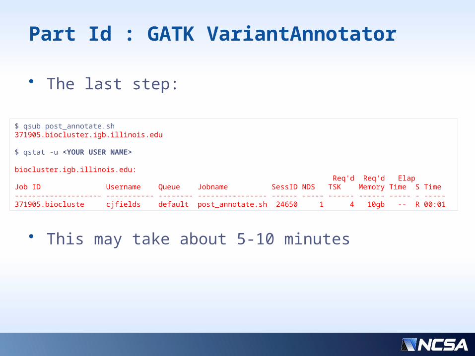
• The last step:
• This may take about 5-10 minutes
$ qsub post_annotate.sh371905.biocluster.igb.illinois.edu
$ qstat -u <YOUR USER NAME>
biocluster.igb.illinois.edu: Req'd Req'd ElapJob ID Username Queue Jobname SessID NDS TSK Memory Time S Time-------------------- ----------- -------- ---------------- ------ ----- ------ ------ ----- - -----371905.biocluste cjfields default post_annotate.sh 24650 1 4 10gb -- R 00:01
While this is going on…
• Let’s start a little tutorial on the Integrated Genome Viewer (also from Broad)

Prelude to Part II
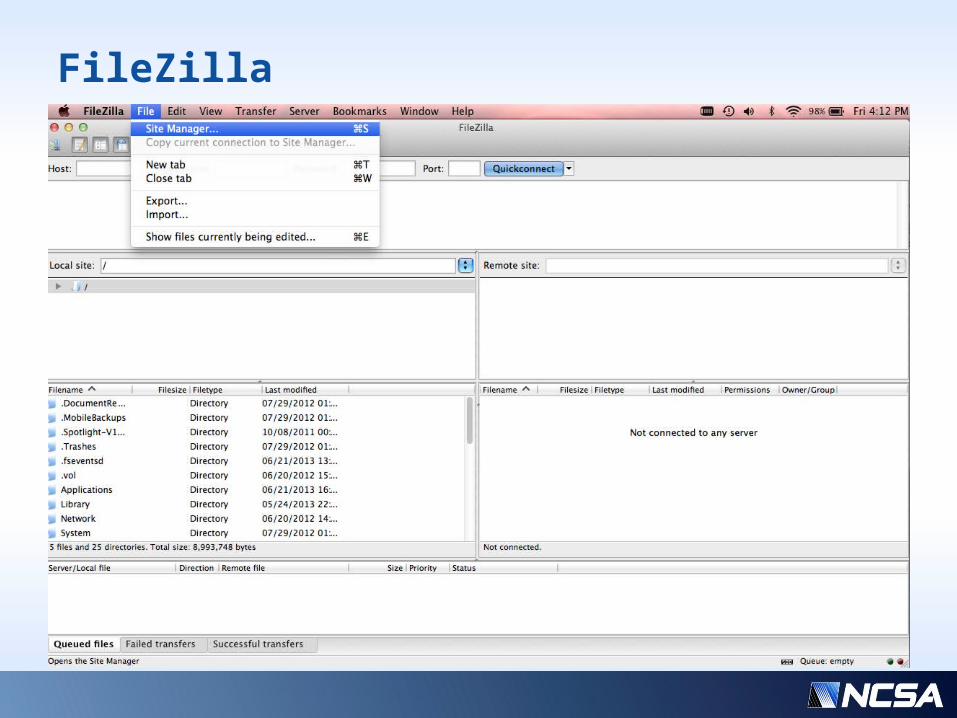
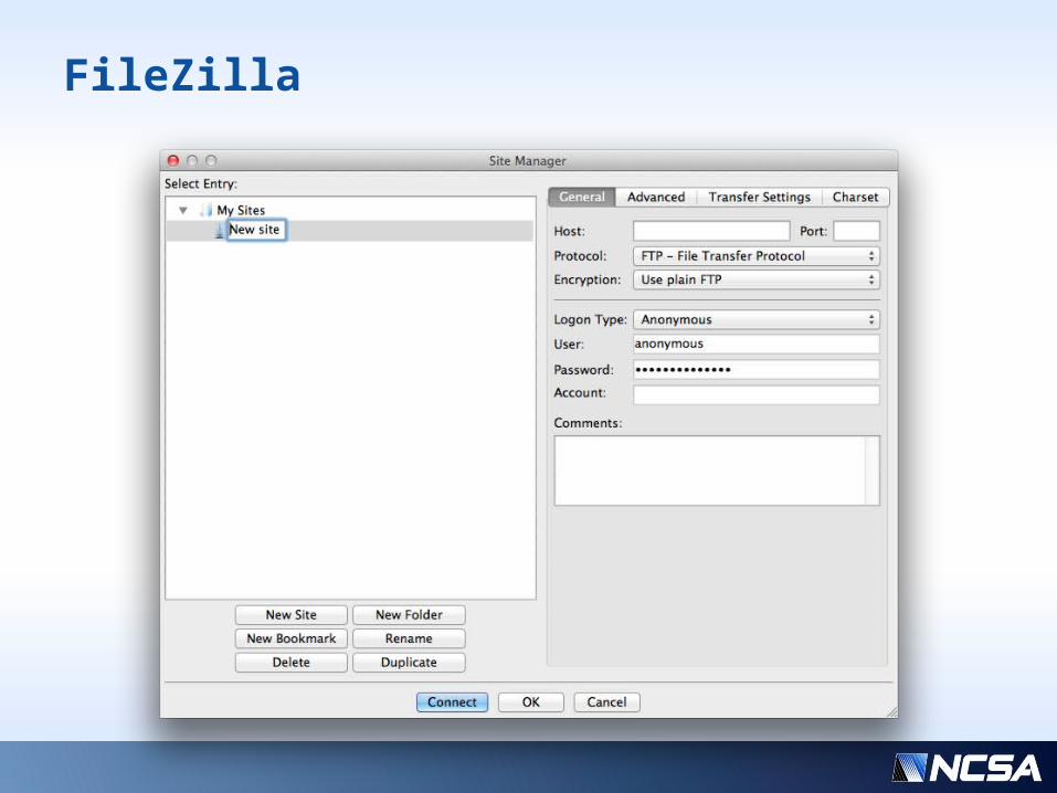
• We need to download the results from your user folders to the local desktop
• We’ll use FileZilla for this
FileZilla

FileZilla
FileZilla

FileZilla

FileZilla

FileZilla
• Transfer folder to the desktop

Part II : Viewing Results in IGV
• Open IGV• Switch genome to ‘Human (b37)’

Part II : Viewing Results in IGV
• Load the VCF files marked ‘final’
• Click on the ‘20’ (chr 20)
Part II : Viewing Results in IGV
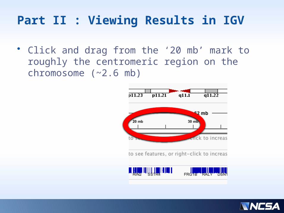
• Click and drag from the ‘20 mb’ mark to roughly the centromeric region on the chromosome (~2.6 mb)

Part II : Viewing Results in IGV
• Click and drag from the ‘20 mb’ mark to roughly the centromeric region on the chromosome (~2.6 mb)

Part II : Viewing Results in IGV
• Should look something like this:

Part II : Viewing Results in IGV
• Right click on the track to bring up a menu, and then select ‘Set Feature Visibility Window’
• Set to ‘10000000’ (10 million, or 10 mb)

Part II : Viewing Results in IGV
• In the search box, enter in ‘FOXA2’
• Browser jumps to that gene

Part II : Viewing Results in IGV
• How many SNPs are here?
• How many indels?
• How many SNPs are ‘hets’?

Part II : Viewing Results in IGV
• Now we’ll load in a ‘small’ BAM file.• This is the same BAM
file you analyzed on the cluster
• In the ‘gatk_bundle’ folder there is a BAM file named ‘NA12878.HiSeq.WGS.bwa.cleaned.recal.b37.20_arm1.
bam’. Load that file. What is happening here?

Part II : Viewing Results in IGV
• Right click on BAM track and select ‘Show coverage track’
• Note colors in coverage track

Part II : Viewing Results in IGV
• Right click on BAM track and select ‘Show coverage track’
• Note colors in coverage track
Part II : Viewing Results in IGV
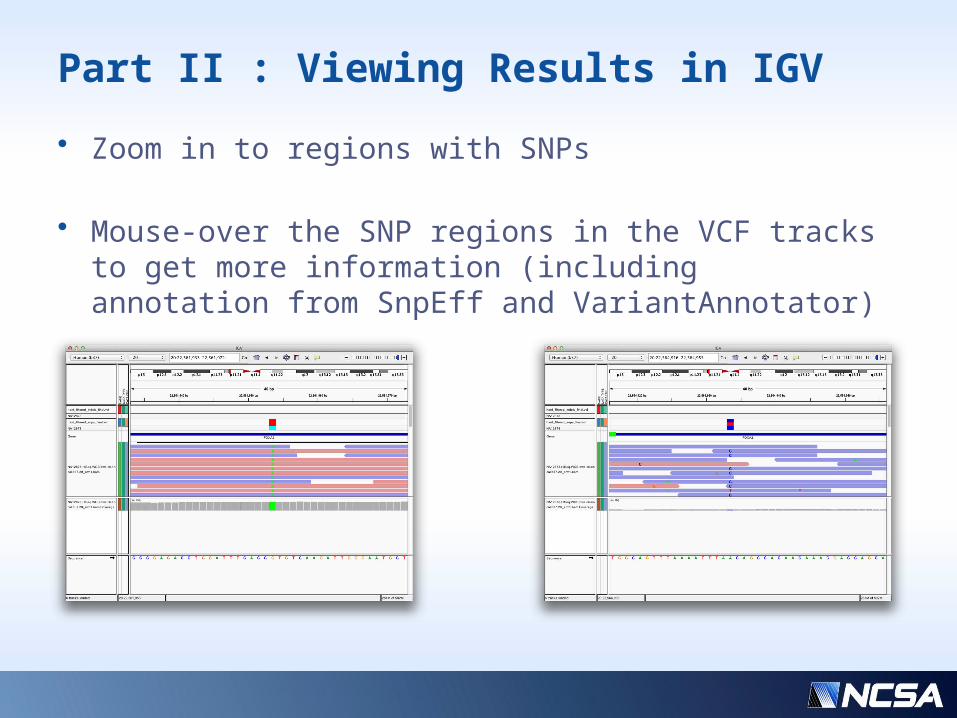
• Zoom in to regions with SNPs
• Mouse-over the SNP regions in the VCF tracks to get more information (including annotation from SnpEff and VariantAnnotator)

Browse around…
• How are filtered SNPs are displayed?
• How about low-quality bases?
• Can you change the display to…• Sort BAM reads by strand?

Part III : SnpEff Results
• SnpEff gives a nice summary HTML file that should have been downloaded with your result (one for SNP, one for indel results)
• Open those up in a browser.