nationwide survey of airborne mercury in finland - borenv.net · ties such as the us food and drug...

Boreal environment research 19 (suppl. B): 355–367 © 2014issn 1239-6095 (print) issn 1797-2469 (online) helsinki 30 september 2014

Editor in charge of this article: Veli-Matti Kerminen

nationwide survey of airborne mercury in Finland

Katriina Kyllönen*, Jussi Paatero, tuula aalto and hannele hakola

Finnish Meteorological Institute, P.O. Box 503, FI-00101 Helsinki, Finland (*corresponding author’s e-mail: [email protected])

Received 5 Aug. 2013, final version received 8 Apr. 2014, accepted 9 May 2014

Kyllönen, K., Paatero, J., aalto, t. & hakola, h. 2014: nationwide survey of airborne mercury in Finland. Boreal Env. Res. 19 (suppl. B): 355–367.

Continuous measurements of total gaseous mercury (TGM) at an urban background station in Helsinki, Finland, were performed in 2006–2007. Additionally, a one-month campaign to measure TGM continuously from a moving car was organized in 2007, when several cities and industrial areas around Finland were surveyed. In Helsinki, a one-year average of 1.54 ± 0.20 ng m–3 was measured, which is about the global average for this persistent pollutant. The highest concentrations, up to 2500 ng m–3, were measured during firing practice that took place next to the station. Seasonal and diurnal variation was studied, and trajectory maps were constructed to analyze mercury source regions. In the mobile meas-urement campaign, concentrations varying between 1.0 and 13.8 ng m–3 were measured. The highest concentrations (above 10 ng m–3) were recorded close to former chlor-alkali plants that used mercury in their electrolytic production process.

Introduction

Mercury is a naturally-occurring element that is ubiquitous around the globe. It is a long-lived pollutant that can bio-accumulate in ecosystems and have adverse effects on human health, espe-cially on children and the developing foetus. In the atmosphere, mercury is mostly present in its elemental form, Hg0. Fish consumption is the primary source of mercury for many popu-lations. Due to bacterial activity in waterbod-ies, inorganic mercury can be transformed into highly toxic methyl mercury, and end up in the fish humans consume. Thus, food safety authori-ties such as the US Food and Drug Adminis-tration and the Finnish Food Safety Authority (Evira) issue consumer advisories about mer-cury in fish and shellfish. Recently, mercury has gained much international attention due to the

launch of new legislation (European Parliament, Council 2004), concerns in the Arctic (AMAP 2011) and, most recently, the UNEP Global Legally Binding Treaty on Mercury that is open for signature by governments in October 2013.

At the global scale, there are several anthro-pogenic sources of mercury, mainly coal com-bustion, small-scale gold mining, manufacturing of non-ferrous metals, cement production, waste disposal and caustic soda production (Pirrone et al. 2010). In Europe, major contributors are the combustion of coal in power plants and resi-dential heat furnaces (~50%), the production of caustic soda using the Hg cell process (17%) and cement production (13%) (Pacyna et al. 2006b). Mercury can also be emitted from natural sources such as waterbodies, soil and vegetation. Re-emission of earlier-deposited mercury affects the mercury budget greatly, although it is extremely

356 Kyllönen et al. • Boreal env. res. vol. 19 (suppl. B)

difficult to quantify (Pacyna et al. 2006a). It has been estimated that natural sources plus re-emission account for two-thirds of total Hg emissions, while anthropogenic sources explain the remaining one-third (Pirrone et al. 2010). In Finland, combustion in the energy, transfer and manufacturing industries and production pro-cesses were the main Hg emission sources in the 1990s (Melanen et al. 1999, Mukherjee et al. 2000). Nowadays according to the national pol-lutant emission database, a single steel-making plant, numerous power plants and the national chemical industry are the main Hg emitters. As estimated by Travnikov et al. (2012), domestic (vs. foreign) Hg emission sources contribute about one-third of the mercury anthropogenic deposition in Finland.

In urban environments, TGM concentra-tions were measured at different locations in e.g. Canada, China, Korea, Mexico, Sweden, Taiwan and the USA (Feng et al. 2004, Poissant et al. 2005, Stamenkovic et al. 2007, Kim et al. 2009, Li et al. 2009, Peterson et al. 2009, Rutter et al. 2009, Liu et al. 2010, Huang et al. 2012, Zhu et al. 2012, Jen et al. 2013). Measurements close to anthropogenic point sources were carried out to a lesser degree, but studies close to chlor-alkali plants, in particular, were made in Belgium, France, Sweden and the USA (Dommergue et al. 2002, Wängberg 2003, 2005, Landis et al. 2004, De Temmerman et al. 2007). However, data from urban and industrial environments in Europe are scarce; moreover, published data on Finnish background or urban mercury concentra-tions in the atmosphere are almost nonexistent.

This paper describes the TGM levels the Finnish public is exposed to in its daily life. Measurements were conducted for one year at an urban background station and also in several cities and industrial areas around the country using a mobile measurement method. These data sets for TGM in Finland are by far the largest so far published. Mobile air quality measurements had been conducted earlier. In Finland, studies with a “Sniffer” Mobile Laboratory Vehicle were carried out several times, but these campaigns did not measure mercury (Pirjola et al. 2004, 2009, 2012). To our knowledge, this is the first time TGM was measured continuously from a moving car.

Experimental sites and methods

Measurement sites

Total gaseous mercury in the ground-level air was measured between September 2006 and August 2007 at the Isosaari weather station (60°06´16´´N, 25°04´05´´E; WMO number 02988). The station is located on the Baltic Sea island of Isosaari about 8 km south-east from the shore of the Helsinki city centre (Fig. 1). The island (76 hectares) is covered mainly by conif-erous forests. However, the station is located on a rocky cape with hardly any vegetation. Isosaari is governed by the Finnish Defence Forces and is closed to the public. The operation of the gar-rison, with occasional firing exercises, is practi-cally the only human activity on the island. The site is categorised as an urban background sta-tion for Helsinki. The weather station was also operated by the military during the measurement period.

A nation-wide survey of the total gaseous mercury in Finland was accomplished with a one-month mobile measurement campaign (henceforth referred to as the MMC) in 2007. All major population centres and a large number of industrial sites were surveyed. The industrial sites visited included e.g. former chlor-alkali plants, power plants and pulp and paper mills.

Sampling

Sampling was conducted using a Tekran 2537A mercury analyser. This instrument collects sam-ples in turns into two gold cartridges at 5-minute intervals, and analyses them continuously. While one cartridge is collecting a sample, the other is being desorbed and the mercury in the sample is analysed by atomic fluorescence spectrometry (AFS). The analyser collects only total gaseous mercury, not particles: these are removed from the sample flow with a PTFE filter. The method has a detection limit of 0.1 ng m–3, repeatability of 2% and a measurement uncertainty of 10%. The analyser was calibrated daily with its inter-nal permeation source at the Isosaari site. During the MMC, the analyser was calibrated at the start of each measurement day and, if needed, later

Boreal env. res. vol. 19 (suppl. B) • Nationwide survey of airborne mercury in Finland 357

during the day. Even in the car, the calibrations were stable with a relative standard deviation of 5%. During the MMC, only two routine calibra-tions were omitted from the whole data set but later on the same day they were successfully carried out. A detailed description of the instru-ment can be found in Kyllönen et al. (2012). This instrument model was used successfully at a number of locations around the world, and has been found to give results comparable to those from other methods (Ebinghaus et al. 1999).

During the MMC, the Tekran mercury ana-lyser described above was installed in a car. This measuring method does not necessarily give information about the typical TGM concentra-tion level in the studied area, since the data are based on 5-min samples provided by Tekran. It rather gives valuable information about possible source areas around the country in a reason-ably short time, and gives an indication of the Hg pollution level in various parts of Finland. When a possible source was identified, meas-urements were conducted in the nearby area for an extended time. Electrical power for the equipment was obtained from the car battery via a 12VDC/230VAC inverter. The sampling line inlet was above the car roof ahead of the posi-tion of the car’s exhaust pipe. Thus ingestion of exhaust fumes into the analyser was prevented when the car was moving.

Concentration fields

Trajectories, i.e. the paths of air parcels arriv-ing at Helsinki, were utilized in an analysis of the long-range transport of mercury. They were calculated five days backwards using a three-dimensional kinematic FLEXTRA trajectory model (e.g. Stohl et al. 1995, Stohl and Seibert 1998), using numerical meteorological data from the European Centre for Medium-Range Weather Forecasts (ECWMF) MARS database. Trajecto-ries were calculated at three-hour intervals, their arrival level at Helsinki being 950 hPa. Trajecto-ries were applied to construct maps of mercury source regions. In this method, the concentra-tion observations are distributed along the cor-responding trajectory paths (Stohl 1996). In the first step, the measured TGM concentrations are

distributed evenly along the path and averaged at every grid point crossed by several paths and thus multiple concentration values. Concentra-tions are scaled and redistributed again along the trajectory path following the methods devel-oped by Stohl (1996). Redistribution continues until the change in the resulting concentration field is negligible. Finally, a chart is obtained where high-concentration regions refer to mul-tiple occasions of air masses with elevated con-centrations passing that region before arriving at Helsinki. Trajectory altitudes < 1000 m were included in order to allow only transport inside the boundary layer and continuous contact with the surface sources.

Results and discussion

One-year study of TGM in Helsinki

The hourly TGM concentrations in the ambient air at the urban background station in Helsinki (Fig. 2) remained mostly close to the global background value of 1.7 ng m–3 for the north-

Fig. 1. location of the measurement site at isosaari.


ern hemisphere (Slemr et al. 2003). During the campaign, the average hourly TGM concentra-tion was 1.54 ± 0.20 ng m–3. Closeness to both local pollution sources (the city of Helsinki) and neighbouring countries with high mercury emis-sions are reflected in the frequent peaks in the data. Hourly concentrations above 3 ng m–3 were seen only on three days during the project.

In August, a pollution plume arrived from the east, resulting in short-term concentrations of up to 14.9 ng m–3 and an hourly concentration of up to 6.5 ng m–3. According to NOAA HYSPLIT backward trajectories, the air masses arrived from Russia and northeast Estonia, and reached mainland Helsinki just before reaching the sta-tion. In Estonia, a power generation complex with the world’s largest oil-shale-fired thermal power plants is located in the northeastern part of the country. Oil shale burning is known to emit significant amounts of Hg into the atmos-phere (Aunela-Tapola et al. 1998). In the TGM data of the Finnish EMEP station at Virolahti, we noticed that when elevated TGM concentrations are observed, the typical source area according to the NOAA HYSPLIT back-trajectories seems to be in northern Estonia (data not published). It remains unclear whether the high TGM values at Isosaari in August resulted from a pollution plume from local sources or from further afield, possibly Estonia.

In May, concentrations above 100 ng m–3 were detected during a two-day period. At first, they were thought to be due to an instrumental

failure, since such concentrations are not likely to be measured at background stations (Munthe et al. 2003, Kim et al. 2005). Closer inspection of the activities at the site showed that, unbe-known to us, target practice took place next to the station at exactly the same time as the elevated concentrations were measured. This led to the conclusion that mercury might originate from the shooting activities. In the firing prac-tice, five 12.7 mm anti-aircraft machine guns were operated. We believe that the TGM origi-nated from mercury fulminate in the rounds shot during the training. Mercury fulminate is a primary explosive and has been used widely in the past. Today, mercury fulminate has been replaced in primers by more efficient chemical substances such as lead compounds, but in mili-tary training old rounds are still used. On the first day, the 5-min concentrations had risen to 280 ng m–3, and then returned to and remained at the background level of 1.4–1.9 ng m–3 during the night, and then skyrocketed again in the morn-ing shortly after the firing resumed. The high-est concentrations occurred during the second day, with values above 1000 ng m–3 for several hours, maximum value being 2470 ng m–3. After the second day of firing practice, the concen-trations did not return to the background level until the sample line filter was replaced. We believe that the firing released huge amounts of particulate mercury in addition to TGM over-loading the filter with particulate Hg (and pos-sibly RGM trapped in the filter), which slowly

0

1

2

3

4

5

6

7

1.IX.2006 1.XI.2006 1.I.2007 3.III.2007 3.V.2007 3.VII.2007 2.IX.2007

TGM

(ng

m–3

) 0

500

1000

1500

2000

1.V.07 1.VI.07

Fig. 2. hourly tGm con-centrations in helsinki. two peaks exceeding the scale, and presented in the smaller figure, repre-sent data during the firing practice.


transformed from the particulate form into the gaseous state. Wallace (1998) showed that when mercury-containing ammunition is used, 86% of the mercury is released mainly via the muzzle, of which 17%–20% was particulate, which sup-ports our conclusion. Although Wallace (1998) reported that only a small percentage of mercury was deposited on the gun operator, our results indicate a possible health concern for the con-scripts and especially for the military staff who regularly attend firing practices. For example, in the study by Munthe et al. (2003) similar to ours Hg concentrations (1.4–26.9 µg m–3) were measured in flue gas from five coal-fired (three hard coal and two brown coal) power plants. In a study by Frey and Hillamo (2011), TGM concen-trations were measured in the raw flue gas of a coal-fired power plant in Helsinki and they were lower than those we measured during the firing practice maxima.

The average TGM concentrations remained stable throughout the year (Table 1), and their variability was small. In summer, when the con-sumption of energy is reduced resulting in less Hg emissions, a slightly smaller average concen-tration was recorded. The data collected during the firing practice were omitted from the spring average value, since the huge concentrations affected the average clearly (see Table 1).

The diurnal variation of TGM was calculated as monthly means for each hour, and proved to be very small. During the cold season (Oct–Mar), there is practically no diurnal variation while in the warm season (Apr–Aug) slight differences were seen. At midnight and during the early morning hours, the concentrations were typically ~0.2 ng m–3 higher than in the afternoon. This tendency is the opposite to that

found at a forested background site in Finland (Kyllönen et al. 2012). In Helsinki, the concen-tration pattern in the warm season was opposite to that of air temperature and wind speed. In the cold season, the temperature and wind speed patterns were not as evident. On calm summer nights, mercury emitted from the sea and the soil around the station accumulates in the stable surface air and is then mixed in the morning as the wind speed increases and solar radiation breaks the surface inversion. In the cold season, the ice and snow covers inhibit this effect. Addi-tionally, thermal mixing increases the boundary layer depth during the daytime and consequently dilutes TGM concentrations (Lee et al. 1998). Similar behaviour was observed e.g. in a rural region in England (Lee et al. 1998) and at urban sites in China (Feng et al. 2004), Sweden (Li et al. 2008) and the USA (Stamenkovich et al. 2007).

A clear majority (97%) of the hourly TGM concentrations were in the range of 1–2 ng m–3, while 3% of the data were between 2 and 3 ng m–3 (Fig. 3). Hourly concentrations greater than 3 ng m–3 were rare, and if the firing practice data were omitted, they were almost nonexistent.

The TGM data were divided into wind sectors (Fig. 4) with the exception of the data collected during the firing practice. The lowest concen-trations were found, quite unexpectedly, when the wind blew from the east, i.e., from Russia. Several pollutants, e.g., SO2, NOx and PAHs, typically arrive from this direction, St. Petersburg being one of the source areas (Vestenius et al. 2011). However, according to ESPREME (http://espreme.ier.uni-stuttgart.de), the St. Petersburg area is a significant source for mercury emis-sions. As stated earlier in this chapter, a pollution

Table 1. seasonal variation of tGm concentrations (mean ± sD) and meteorological data measured in helsinki from oct 2006 to aug 2007. autumn = oct–nov, winter = Dec–Feb, spring = mar–may, summer = Jun–aug.

autumn Winter spring summer

tGm (ng m–3) 1.57 ± 0.17 1.59 ± 0.12 1.59 ± 0.21 (6.1 ± 81.6)a 1.45 ± 0.29temperature (°c) 5.9 ± 4.30 –0.7 ± 6.50 4.9 ± 3.8 16.3 ± 2.70humidity (%) 87 ± 9.00 85 ± 8.00 79 ± 15 79 ± 12Wind speed (m s–1) 7.8 ± 3.60 8.1 ± 3.40 6.1 ± 2.9 5.5 ± 2.8Precipitation amount (mm) 216 149 84 172

a Firing practice data included.


plume with concentrations above 10 ng m–3 was recorded during prevailing easterly winds. One should note that only 6.9% of the wind factors at the site are related to this low-concentration factor (90°–130°), while typical wind factors are from the west and southwest (45%, 210°–290°). Still, both the median and the 5 and 95 percen-tiles remained mostly low for the ESE sector.

The highest concentrations occurred with winds in the 300°–40° sectors (N factor) and the 160°–240° sector (S factor). The N factor is accounted for by domestic and especially, by close emission sources. Two coal-fired power plants and a natural gas power station are located in Helsinki, and these produce annually approxi-mately 1000 MW of electricity and 1500 MW of municipal heating. The S factor contains pol-luted air masses from the highly-industrialised Baltic and European areas.

To study the source areas for high TGM concentrations in more detail, a TGM concentra-tion field for Isosaari was calculated (Fig. 5). According to the trajectory analysis, the strong-est source areas for Helsinki were located in the densely-populated and industrialized areas of central Europe, and also to some extent in the southern part of eastern Europe. Additionally, there seemed to be a source area in Russia. How-ever, these Russian grid points with high concen-tration values were located on the periphery of the map and the exact location was thus uncer-tain. This source might explain the high 95th percentile for the 80° wind sector (Fig. 4). Low concentrations over the sea and Fenno-Scandina-via resulted from the lack of significant sources in these areas. The TGM concentration field (Fig. 5) resembled the spatial distribution map of mercury emissions over the EMEP domain in 2010 as modelled by EMEP (Travnikov et al. 2012), thus indicating that the hot spot sources detected by trajectory analysis are in line with the anthropogenic emissions.

Since mercury as an airborne pollutant has a rather long lifetime of 0.5–2 years (Schroeder and Munthe 1998), the Hg emissions from neigh-bouring countries affect the ambient air concen-tration levels in Helsinki in addition to domestic Hg emissions. According to ESPREME (http://espreme.ier.uni-stuttgart.de), the total annual emissions in 2000 of Hg in Finland, Estonia, Latvia, Lithuania, Poland and Russia were 0.60, 0.55, 0.15, 0.25, 25.6 and 66.1 t, respectively.

1

10

100

1000

10000

100000

< 1 1 1.2 1.4 1.6 1.8 2 3 4 5 6 7 8 9 > 10

Freq

uenc

y (n

)

TGM (ng m–3) Fig. 3. Frequency pattern of 5-min tGm concentrations in helsinki during the study period. concentrations of 1–2 ng m–3 are at 0.2 ng m–3 intervals (e.g. a bar of 1.2 represents data in the range of 1.20–1.39 ng m–3) while higher concentrations are at 1 ng m–3 intervals.

1.0

1.2

1.4

1.6

1.8

2.0

2.2

10 40 70 100 130 160 190 220 250 280 310 340 360

TGM

(ng

m–3

)

N S WE N

Fig. 4. tGm distribution in different wind sectors. the box represents the 25th and 75th percentiles, the line gives the median con-centrations, and whiskers the 5th and 95th percen-tiles.


Nationwide survey

In the mobile measurement campaign, all the major population centres and a large number of industrial sites were surveyed by online meas-urements from a moving car. Furthermore, most of the municipalities in the country were vis-ited with the exception of the province of Lap-land. The industrial sites visited included e.g. former chlor-alkali plants, power plants, chemi-cal industry and pulp and paper mills.

The measurement days were mostly sunny or cloudy, while rain occurred a few times. During rain showers measurements were stopped to pre-vent water from entering the instrument through the horizontally-placed sampling tube on the roof of the car. In fog, measurements were con-ducted, but concentrations were typically lower than just before or after it. We believe that this phenomenon is caused by gaseous mercury bind-ing to the tiny water droplets, as clouds act as a reaction vessel for aqueous chemistry, influenc-ing the rates at which atmospheric Hg is incor-porated into raindrops (Malcolm et al. 2003) and Hg is accumulated and concentrated in fog banks (Ritchie et al. 2006).

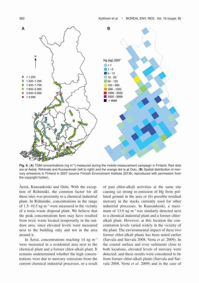
The majority of the measured concentrations remained at a low level, with no clear local influ-ence (Fig. 6A). During the campaign, 89% of the data were below the global average of 1.7 ng m–3 with a median of 1.56 ± 0.91 ng m–3 for the whole data set. The 5th and 95th percentiles of the whole data were 1.13 and 1.97 ng m–3,

respectively, indicating a quite stable TGM con-centration throughout Finland. This is due to the stable behaviour of this element and lack of significant local sources. It was noted that during different measurement days, the concentration levels changed a bit as can be seen in the bluish and greenish routes on the map (see Fig. 6A). This occurrence was also evident in the data from the measurements at the same location on different days. Due to changing wind pat-terns, the effect of long-range transported pol-lution plumes varied. The changes were small though, indicating an effective mixing of this long-life pollutant. Also changing weather (i.e. fog) affected the concentration level, as noted earlier. One must also remember that the instru-ment has a measurement uncertainty of 10%, so that changes of about 0.1 ng m–3 can also be due to instrumental performance.

Only 2% of the data exceeded 3 ng m–3. These events were short and never represented the concentration level in an entire town. These peaks were measured close to an obvious source and remained high only in certain measurement places. Typically, a few hundred metres away from the location of the high TGM concentra-tion, it declined back to the background level. This measurement method may have neglected some hot-spot areas due to unfavorable wind conditions or difficulties in driving to the opti-mal measurement location.

High TGM concentrations (here > 3 ng m–3) were measured in certain areas of Riihimäki,

Fig. 5. tGm concentration field for Helsinki calcu-lated from the hourly tGm concentrations.


Äetsä, Kuusankoski and Oulu. With the excep-tion of Riihimäki, the common factor for all these sites was proximity to a chemical industrial plant. In Riihimäki, concentrations in the range of 1.5–10.5 ng m–3 were measured in the vicinity of a toxic-waste disposal plant. We believe that the peak concentrations here may have resulted from toxic waste located temporarily in the out-door area, since elevated levels were measured next to the building only and not in the area around it.

In Äetsä, concentrations reaching 14 ng m–3 were measured in a residential area next to the chemical plant and a former chlor-alkali plant. It remains undetermined whether the high concen-trations were due to mercury emissions from the current chemical industrial processes, or a result

of past chlor-alkali activities at the same site causing (a) strong re-emission of Hg from pol-luted ground in the area or (b) possible residual mercury in the stacks currently used for other industrial processes. In Kuusankoski, a maxi-mum of 13.0 ng m–3 was similarly detected next to a chemical industrial plant and a former chlor-alkali plant. However, at this location the con-centration levels varied widely in the vicinity of the plant. The environmental impact of these two former chlor-alkali plants has been noted earlier (Sarvala and Sarvala 2008, Verta et al. 2009). In the coastal surface and river sediments close to both locations, elevated levels of mercury were detected, and these results were considered to be from former chlor-alkali plants (Sarvala and Sar-vala 2008, Verta et al. 2009) and in the case of

< 1.2001.200–1.3991.400–1.7991.800–2.9993.000–9.999> 9.999

N

Fig. 6. (A) tGm concentrations (ng m–3) measured during the mobile measurement campaign in Finland. red dots are at Äetsä, riihimäki and Kuusankoski (left to right) and the orange dot is at oulu. (B) spatial distribution of mer-cury emissions in Finland in 2007 (source Finnish environment institute 2013b; reproduced with permission from the copyright holder).

A B


Kuusankoski also from the pulp and paper indus-try (Verta et al. 2009). Despite these findings, in the vicinity of another former chlor-alkali plant in Joutseno no elevated TGM levels were meas-ured as compared with the background concen-tration of 1.5 ng m–3 in the area.

The only chlor-alkali plant remaining in Fin-land is located in an industrial area of Oulu. The area was not accessible by car; concentra-tions up to 4.6 ng m–3 were measured outside the industrial area. Much higher concentrations (around 50–250 ng m–3) were measured in 2001 in the plumes of a chlor-alkali plant in Sweden, 70 m from the source (Wängberg et al. 2003). However, in a residential area 560 m away from the plant, concentrations of 1.4–40 ng m–3 were detected (mean = 3.5 ng m–3) (Wängberg et al. 2005).

Elevated levels were also measured in Hel-sinki, Tampere, Harjavalta, Kokkola, Raahe and Tornio (up to 2.8, 2.0, 2.3, 2.2, 2.1 and 2.7 ng m–3, respectively). These were all detected within industrial areas, or in one case in a resi-dential area. In Helsinki, the areas around cre-matoria were carefully surveyed, but no increase in TGM concentrations were found during the campaign.

The Finnish Environment Institute maintains a national environmental monitoring database VAHTI containing the reports made periodically by individual facilities regarding their pollut-ant (e.g. Hg) emissions. The top five polluters include the steel and chemical industry, while most of the facilities reporting Hg emissions are power plants (data not shown). Globally, coal combustion is the main source of Hg emissions (Pirrone et al. 2010). We could not clearly con-nect power production with elevated concen-tration levels during our mobile measurement campaign. This is likely to be due to effective dilution resulting from the use of tall smoke-stacks in power plants.

Comparison with other studies

There are no published urban or industrial TGM data in Finland with which to compare our meas-urements. In June 1971, particle-bound mercury with an average concentration of 0.28 ng m–3 and

maximum of 1.0 ng m–3 was measured in central Helsinki by the Department of Radiochemistry, University of Helsinki (Miettinen 1973, as cited in Mattsson and Jaakkola 1979). As mercury exists mostly in the gaseous elemental form Hg0 (95%–99%), while mercury associated with particulate matter makes up only 0.2%–1.4% (Ebinghaus et al. 2008), we used a very rough estimating factor of 100 to calculate the TGM concentration in Helsinki in 1971. This would give an approx. mean value of 30 ng m–3 of TGM and a maximum of 100 ng m–3 of TGM in Hel-sinki during that year. These figures are about 20 times higher than the average TGM concentra-tion and seven times higher than the maximum TGM concentration measured in Helsinki during our study. These high concentrations were due to the incineration of unsorted household waste and heating of buildings with coal (Mattsson and Jaakkola 1979). However, these values are uncertain, since the ratio between TGM and particle-bound mercury may then have been smaller, and the measurement method did not take into account the problem of mercury inter-actions with the particles collected on the filter.

Additionally, we made a comparison with recent TGM data from other countries (Table 2) to set the mercury situation in Helsinki into a global perspective. In Asia and Mexico, much higher TGM concentrations are found in urban areas as compared with the sites in Europe and North America. Our results from the one-year study in Helsinki and the mobile measurement campaign around the country, are located in the lower part of those given in the published studies (see Table 2).

Mercury emissions in Finland

According to the national mercury emissions reported by the Finnish Environment Institute (SYKE), during the last two decades Hg emis-sions did not change much. After 1990, the annual emission levels of Hg into the air have been below 1000 kg (Fig. 7, numerical values obtained from the Finnish Environment Institute 2013a). In recent years, emissions have remained rather steady, although unfortunately at the same level as in the early 1990s. The time series is not


Table 2. summary of tGm (or gaseous elemental mercury, Gem) measurements in urban areas and close to point sources.

location site Year Period mean ± sD (min–max) reference tGm or Gem (ng m–3)

helsinki, Finland Urban 2006–2007 11 months 1.54 ± 0.20 (0.86–14.9) our study,Finland* industrial, urban, part 1 background 2007 1 month (0.97–13.75) our study, part 2taiwan industrial/urban 2010 7 months 6.66 ± 1.42 Jen et al. (2013)nanjing, china Urban 2011 1 yr 7.9 ± 7.0 (0.8–180) Zhu et al. (2012)taiwan Urban 2010–2011 1 yr 6.14 ± 3.91 huang et al. (2012)Detroit, Usa Urban/industrial 2004 1 yr 2.5 ± 1.4 (0.36-25.6) liu et al. (2010)reno, Usa Urban 2004–2007 3 yr 1.6 ± 0.5 (0.5–6.4) Peterson et al. (2009)seoul, Korea Urban 2005–2006 1 yr 3.22 ± 2.10 Kim et al. (2009)mexico city Urban 2006 1 month 7.2 ± 4.8 rutter et al. (2009)Gothenburg, sweden Urban 2005 1 month 1.96 ± 0.38 li et al. (2008)Belgium industrial 1999–2004 – 20 (max 150) De temmerman et al. (2007)reno, Usa Urban 2002–2005 3 yr 2.3 ± 0.6 (0.9–8.6) stamenkovic et al. (2007)Quebec, canada Urban 2003 1 yr 1.65 ± 0.42 Poissant et al. (2005)Bohus, sweden industrial 2001–2003 10 weeks 55 (1.5–540) Wängberg et al. (2005)Bohus, sweden industrial/urban 2001–2003 10 weeks 3.5 (1.4-40) Wängberg et al. (2005)michigan, Usa industrial (2) 2000 10 days 3.9 and 8.7 (1.9–77.6) landis et al. (2004)Grenoble, France industrial/suburban 1999–2000 40 days 3.4 ± 3.6 (max 45.9) Dommergue et al. (2002)

* comprises several measuring locations around the country.

0

0.2

0.4

0.6

0.8

1

1.2 19

90

1991

19

92

1993

19

94

1995

19

96

1997

19

98

1999

20

00

2001

20

02

2003

20

04

2005

20

06

2007

20

08

2009

20

10

2011

Hg

emis

sion

(t)

Fig. 7. mercury emissions into the air in Finland in 1990–2011.

fully consistent due to the pending recalcula-tion of the energy-sector emissions. According to the European Environment Agency (EEA), a clear decreasing trend in Hg emissions occurred

in Europe in 1990–2010 (European Environ-ment Agency 2014a). Additionally, EEA reports a 20% decrease in the Hg emissions in Finland during the same period (European Environment Agency 2014b). However, even so, this reduc-tion is among the smallest in the EEA Member Countries. In the other Nordic countries, the reduction was substantial (60%–85%).

A map of Hg emissions in 2007 (Fig. 6B) published in Finnish Environment Institute (2013b) shows some resemblance to our map (Fig. 6A), although in certain emission areas we did not detect any increase in TGM concentra-tions. This is likely due to the limitations of our measurement method, addressed earlier in this article.


Conclusions

This study presents the total gaseous mercury (TGM) concentrations in the air in Finland measured during (1) a one-year measurement campaign at an urban background station in Hel-sinki, Finland, to measure TGM concentrations in the air and to study the behaviour of this pol-lutant; and (2) a mobile measurement campaign around Finland to study the regional variation of TGM in urban, industrial and background areas and to find possible Hg hot spots.

The hourly TGM values measured during the one-year urban campaign mostly remained close to the global background value, with an average of 1.54 ± 0.20 ng m–3. Proximity to both local pollution sources (city of Helsinki) and neigh-bouring countries with high mercury emissions was reflected in the frequent peaks in the data. The seasonal variation of TGM concentrations was small, however slightly smaller than average concentrations were measured in summer due to less energy consumption. A diurnal variation was observed during the warm season (Apr–Aug) with a peak at night or during early morning hours. Values above 1000 ng m–3 were detected for several hours on one measurement day when, a firing practice took place next to the station.

During the mobile measurement campaign, the highest concentrations (10–15 ng m–3) were measured in the immediate vicinity of certain chemical manufacturing plants formerly used in chlor-alkali industry, and a toxic waste disposal plant. In other industrial areas or residential areas close to industry, the TGM concentrations were less than 5 ng m–3. In general, the measured concentrations were low, with a median of 1.43 ng m–3, and elevated levels of TGM could not be connected to power plant emissions or crematoria.

The results from these campaigns indicate that the domestic anthropogenic emissions are only a minor source of mercury exposure to the general public in Finland.

Acknowledgements: This project was partially funded by the Ministry of the Environment. The authors are grateful for the support by The Finnish Defence Forces officers and conscripts at the Isosaari military base. Map production assistance by Mr. Pentti Pirinen, FMI, is gratefully acknowl-edged. Additionally we thank Ms. Kristina Saarinen, SYKE, for help with interpretation of emission data.

References

AMAP 2011. AMAP assessment 2011: Mercury in the Arctic. Arctic Monitoring and Assessment Programme (AMAP), Oslo, Norway.

Aunela-Tapola L.A., Frandsen F.J. & Häsänen E.K. 1998. Trace metal emissions from the Estonian oil shale fired power plant. Fuel Processing Technology 57: 1–24.

De Temmerman L., Claeys N., Roekens E. & Guns M. 2007. Biomonitoring of airborne mercury with perennial ryegrass cultures. Environ. Poll. 146: 458–462.

Dommergue A., Ferrari C.P., Planchon F.M.A. & Boutron C.F. 2002. Influence of anthropogenic sources on total gaseous mercury variability in Grenoble suburban air (France). Sci. Total Environ. 297: 203–213.

Ebinghaus R., Jennings S.G., Schroeder W.H., Berg T., Don-aghy T., Guentzel J., Kenny C., Kock H.H., Kvietkus K., Landing W., Mühleck T., Munthe J., Prestbo E.M., Schneeberger D., Slemr F., Sommar J., Urba A., Walls-chläger D. & Xiao Z. 1999. International field intercom-parison measurements of atmospheric mercury species at Mace Head, Ireland. Atmos. Environ. 33: 3063–3073.

Ebinghaus R., Banic C., Beauchamp S., Jaffe D., Kock H.H., Pirrone N., Poissant L., Sprovieri F. & Weiss P.S. 2008. Spatial coverage and temporal trends of land-based atmospheric mercury measurements in the northern and southern hemispheres. In: Pirrone N. & Mason R. (eds.), Mercury fate and transport in the global atmosphere: measurements, models and policy implications, Springer Science + Business Media, New York, pp. 168–219.

European Environment Agency 2014a. Change in cadmium, mercury and lead emissions for each sector between 1990 and 2010 (EEA member countries). Available at http://www.eea.europa.eu/data-and-maps/daviz/change-in-cadmium-mercury-and#tab-chart_1.

European Environment Agency 2014b. The reported change in mercury (Hg) emissions for each country, 1990–2010. Available at http://www.eea.europa.eu/data-and-maps/figures/change-in-mercury-emissions-1990-2007-eea-member-countries-3.

European Parliament, Council 2004. Directive 2004/107/EC of the European Parliament and of the Council of 15 December 2004 relating to arsenic, cadmium, mercury, nickel and polycyclic aromatic hydrocarbons in ambient air. Official Journal of the European Union L23: 3–16.

Feng X., Shang L., Wang S., Tang S. & Zheng W. 2004. Temporal variation of total gaseous mercury in the air of Guiyang, China. J. Geophys. Res. 109, D03303, doi:10.1029/2003JD004159.

Finnish Environmental Institute 2013a. Air pollutant emis-sions in Finland. Available at http://www.ymparisto.fi/en-US/Maps_and_statistics/Air_pollutant_emissions.

Finnish Environmental Institute 2013b. Spatial distribution of air pollutant emissions in Finland. Available at http://www.ymparisto.fi/en-us/Maps_and_statistics/Air_pol-lutant_emissions/Spatial_distribution_of_air_pollutant_emissions.

Frey A. & Hillamo R. 2011. Fine particle emissions of a heavy fuel oil-fired heating station and a coal-fired power plant: Helsinki Energy Research report. Internal


report 11/2011, Helsinki Energy.Helsingin Energia 2010. Power plants. Available at http://

www.helen.fi/en/Households/Information/Energy-and-the-environment/Energy-production/Power-plants/.

Huang J., Liu C.K., Huang C.S. & Fang G.C. 2012. Atmos-pheric mercury pollution at an urban site in central Taiwan: Mercury emission sources at ground level. Che-mosphere 87: 579–585.

Jen Y.H., Yuan C.S., Hung C.H., Ie I.R. & Tsai C.M. 2013. Tempospatial variation and partition of atmospheric mercury during wet and dry seasons at sensitivity sites within a heavily polluted industrial city. Aerosol Air Qual. Res. 13: 13–23.

Kim K.H., Ebinghaus R., Schroeder W.H., Blanchard P., Kock H.H., Steffen A., Froude F.A., Kim M.Y., Hong S. & Kim J.H. 2005. Atmospheric mercury concentrations from several observatory sites in the northern hemi-sphere. J. Atmos. Chem. 50: 1–24.

Kim S.H., Han Y.J., Holsen T.M. & Yi S.M. 2009. Character-istics of atmospheric speciated mercury concentrations (TGM, Hg(II) and Hg(p)) in Seoul, Korea. Atmos. Envi-ron. 43: 3267–3274.

Kyllönen K., Hakola H., Hellén H., Korhonen M. & Verta M. 2012. Atmospheric mercury fluxes in southern boreal forest and wetland. Water Air Soil Pollut. 223: 1171–1182.

Landis M.S., Keeler G.J., Al-Walib K.I. & Stevens R.K. 2004. Divalent inorganic reactive gaseous mercury emissions from a mercury cell chlor-alkali plant and its impact on near-field atmospheric dry deposition. Atmos. Environ. 38: 613–622.

Li J., Sommar J., Wängberg I., Lindqvist O. & Wei S. 2008. Short-time variation of mercury speciation in the urban of Göteborg during GÖTE-2005. Atmos. Environ. 42: 8382–8388.

Liu B., Keeler G.J., Dvonch J.T., Barres J.A., Lynam M.M., Marsik F.J. & Morgan J.T. 2010. Urban-rural differences in atmospheric mercury speciation. Atmos. Environ. 44: 2013–2023.

Malcolm, E.G., Keeler G.J., Lawson S.T. & Sherbatskoy T.D. 2003. Mercury and trace elements in cloud water and precipitation collected on Mt. Mansfield, Vermont. J. Environ. Monit. 5: 584–590.

Mattsson R. & Jaakkola T. 1979. An analysis of Helsinki air 1962 to 1977 based on trace metals and radionuclides. Geophysica 16: 1–42

Munthe J., Wängberg I., Iverfeldt Å., Lindqvist O., Ström-berg D., Sommar J., Gårdfeldt K., Petersen G., Ebing-haus R., Prestbo E., Larjava K. & Siemens V. 2003. Distribution of atmospheric mercury species in Northern Europe: final results from the MOE project Atmos. Envi-ron. 37, Suppl. 1: S9–S20.

Pacyna E.G., Pacyna J.M., Steenhuisen F. & Simon Wilson S. 2006a. Global anthropogenic mercury emission inventory for 2000. Atmos. Environ. 40: 4048–4063.

Pacyna E.G., Pacyna J.M., Fudala J., Strzelecka-Jastrzab E., Hlawiczka S. & Panasiuk D. 2006b. Mercury emissions to the atmosphere from anthropogenic sources in Europe in 2000 and their scenarios until 2020. Sci. Total Envi-ron. 370: 147–156.

Pirjola L., Parviainen H., Hussein T., Valli A., Hämeri K.,

Aalto P., Virtanen A., Keskinen J., Pakkanen T.A., Mäkelä T. & Hillamo R.E. 2004. ‘‘Sniffer’’— a novel tool for chasing vehicles and measuring traffic pollut-ants. Atmos. Environ. 38: 3625–3635.

Pirjola L., Kupiainen K.J., Perhoniemi P., Tervahattu H. & Vesala H. 2009. Non-exhaust emission measurement system of the mobile laboratory SNIFFER. Atmos. Envi-ron. 43: 4703–4713.

Pirjola L., Lahde T., Niemi J.V., Kousa A., Ronkko T., Kar-jalainen P., Keskinen J., Frey A. & Hillamo R. 2012. Spatial and temporal characterization of traffic emissions in urban microenvironments with a mobile laboratory. Atmos. Environ. 63: 156–167.

Pirrone N., Cinnirella S., Feng X., Finkelman R. B., Friedli H. R., Leaner J., Mason R., Mukherjee A.B., Stracher G.B., Streets D.G. & Telmer K. 2010. Global mer-cury emissions to the atmosphere from anthropogenic and natural sources. Atmos. Chem. Phys. Discuss. 10: 4719–4752.

Poissant L., Pilote M., Beauvais C., Constant P. & Zhang H.H. 2005. A year of continuous measurements of three atmos-pheric mercury species (GEM, RGM and Hgp) in south-ern Québec, Canada. Atmos. Environ. 39: 1275–1287.

Ritchie C.D., Richards W. & Arp P.A. 2006. Mercury in fog on the Bay of Fundy (Canada). Atmos. Environ. 40: 6321–6328.

Rutter A.P., Snyder D.C., Stone E.A., Schauer J.J., Gonzalez-Abraham R., Molina L.T., Márquez C., Cárdenas B. & de Foy B. 2009. In situ measurements of speciated atmospheric mercury and the identification of source regions in the Mexico City Metropolitan Area. Atmos. Chem. Phys. 9: 207–220.

Sarvala M. & Sarvala J. (eds.) 2005. Miten voit, Selkämeri? Ympäristön tila Lounais-Suomessa 4, Lounais-Suomen ympäristökeskus, Turku.

Schroeder W. & Munthe J. 1998. Atmospheric mercury — an overview. Atmos. Environ. 32: 809–822.

Slemr F., Brunke E.-G., Ebinghaus R., Temme C., Munthe J., Wängberg I., Schroeder W., Steffen A. & Berg T. 2003. Worldwide trend of atmospheric mercury since 1977. Geo-phys. Res. Lett. 30, 1516, doi:10.1029/2003GL016954.

Stamenkovic J., Lyman S. & Gustin M.G. 2007. Seasonal and diel variation of atmospheric mercury concentra-tions in the Reno (Nevada, USA) airshed. Atmos. Envi-ron. 41: 6662–6672.

Stohl A., Wotawa G., Seibert P. & Kromp-Kolb H. 1995. Interpolation errors in wind fields as a function of spatial and temporal resolution and their impact on different types of kinematic trajectories. J. Appl. Meteorol. 34: 2149–2165.

Stohl A. 1996. Trajectory statistics — a new method to estab-lish source–receptor relationships of air pollutants and its application to the transport of particulate sulfate in Europe. Atmos. Environ. 30: 579–587.

Stohl A. & Seibert P. 1998. Accuracy of trajectories as deter-mined from the conservation of meteorological tracers. Q. J. R. Meteor. Soc. 124: 1465–1484.

Travnikov O., Ilyin I., Rozovskaya O., Varygina M., Aas W., Uggerud H.T., Mareckova K. & Wankmueller R. 2012. Long-term changes of heavy metal transboundary pol-


lution of the environment (1990–2010). EMEP Status Report 2/2012.

Verta M., Kiviranta H., Salo, S., Malve O., Korhonen M., Verkasalo P.K., Ruokojärvi P., Rossi E., Hanski A., Päätalo K. & Vartiainen T. 2009. A decision framework for possible remediation of contaminated sediments in the River Kymijoki, Finland. Environ Sci. Pollut. Res. Int. 16: 95–105.

Vestenius M., Leppänen S., Anttila P., Kyllönen K., Hat-akka J., Hellén H., Hyvärinen A. & Hakola H. 2011. Background concentrations and source apportionment of polycyclic aromatic hydrocarbons in south-eastern Finland. Atmos. Environ. 45: 3391–3399.

Wallace J.S. 1998. Discharge residue from mercury fulmi-

nate-primed ammunition. Science & Justice 38: 7–14Wängberg I., Edner H., Ferrara R., Lanzillotta E., Munthe

J., Sommar J., Sjöholm M., Svanberg S. & Weibring P. 2003. Atmospheric mercury near a chlor-alkali plant in Sweden. Sci. Total Environ. 304: 29–41.

Wängberg I., Barregard L., Sällsten G., Haeger-Eugensson M., Munthe J. & Sommar J. 2005. Emissions, dispersion and human exposure of mercury from a Swedish chlor-alkali plant. Atmos. Environ. 39: 7451–7458.

Zhu J., Wang T., Talbot R., Mao H., Hall C.B., Yang X., Fu C., Zhuang B., Li S., Han Y. & Huang X. 2012. Charac-teristics of atmospheric Total Gaseous Mercury (TGM) observed in urban Nanjing, China. Atmos. Chem. Phys. 12: 12103–12118.

nationwide survey of airborne mercury in finland - borenv.net · ties such as the us food and drug...

Documents