naval postgraduate schools) john a. lukacs iv 5. funding numbers 7. performing organization name(s)...

NAVAL

POSTGRADUATE SCHOOL

MONTEREY, CALIFORNIA

THESIS

HIT-TO-KILL GUIDANCE ALGORITHM FOR THE INTERCEPTION OF BALLISTIC MISSILES IN THE

BOOST PHASE

by

John A. Lukacs IV

June 2006

Thesis Advisor: Oleg Yakimenko

Approved for public release; distribution is unlimited.

THIS PAGE INTENTIONALLY LEFT BLANK

i

REPORT DOCUMENTATION PAGE Form Approved OMB No. 0704-0188 Public reporting burden for this collection of information is estimated to average 1 hour per response, including the time for reviewing instruction, searching existing data sources, gathering and maintaining the data needed, and completing and reviewing the collection of information. Send comments regarding this burden estimate or any other aspect of this collection of information, including suggestions for reducing this burden, to Washington headquarters Services, Directorate for Information Operations and Reports, 1215 Jefferson Davis Highway, Suite 1204, Arlington, VA 22202-4302, and to the Office of Management and Budget, Paperwork Reduction Project (0704-0188) Washington DC 20503. 1. AGENCY USE ONLY (Leave blank)

2. REPORT DATE June 2006

3. REPORT TYPE AND DATES COVERED Master’s Thesis

4. TITLE AND SUBTITLE Hit-to-Kill Guidance Algorithm for the Interception of Ballistic Missiles During the Boost Phase 6. AUTHOR(S) John A. Lukacs IV

5. FUNDING NUMBERS

7. PERFORMING ORGANIZATION NAME(S) AND ADDRESS(ES) Naval Postgraduate School Monterey, CA 93943-5000

8. PERFORMING ORGANIZATION REPORT NUMBER

9. SPONSORING /MONITORING AGENCY NAME(S) AND ADDRESS(ES) N/A

10. SPONSORING/MONITORING AGENCY REPORT NUMBER

11. SUPPLEMENTARY NOTES The views expressed in this thesis are those of the author and do not reflect the official policy or position of the Department of Defense or the U.S. Government. 12a. DISTRIBUTION / AVAILABILITY STATEMENT Approved for public release; distribution is unlimited.

12b. DISTRIBUTION CODE

13. ABSTRACT (maximum 200 words) A near-optimal guidance law has been developed using the direct method of calculus of variations that maximizes the kinetic energy transfer from a surface-launched missile upon interception to a ballistic missile target during the boost phase of flight. Mathematical models of a North Korean Taep'o-dong II (TD-2) medium-range ballistic missile and a Raytheon Standard Missile 6 (SM-6) interceptor are used to demonstrate the guidance law’s performance. This law will utilize the SM-6’s onboard computer and active radar sensors to independently predict an intercept point, solve the two-point boundary value problem, and determine a near-optimal flight path to that point. Determining a truly optimal flight path would require significant computing power and time, while a near-optimal flight path can be calculated onboard the interceptor and updated in real time without significant changes to the interceptor’s hardware. That near-optimal guidance path is then converted into a set of command functions and fed back into the control computer of the interceptor. By modifying the second and third derivatives of the two-point boundary value problem, the intercept conditions can be varied to study their effects upon the optimal flight path regarding the maximization of kinetic energy upon impact.

15. NUMBER OF PAGES

157

14. SUBJECT TERMS Missile Guidance Laws, Direct Methods, Optimal Control, Boost Phase Intercept, Hit-to-Kill

16. PRICE CODE

17. SECURITY CLASSIFICATION OF REPORT

Unclassified

18. SECURITY CLASSIFICATION OF THIS PAGE

Unclassified

19. SECURITY CLASSIFICATION OF ABSTRACT

Unclassified

20. LIMITATION OF ABSTRACT

UL NSN 7540-01-280-5500 Standard Form 298 (Rev. 2-89) Prescribed by ANSI Std. 239-18

ii


iii

Approved for public release; distribution is unlimited.

HIT-TO-KILL GUIDANCE ALGORITHM FOR THE INTERCEPTION OF BALLISTIC MISSILES IN THE BOOST PHASE

John A. Lukacs IV Lieutenant, United States Navy B.S., Drexel University, 1999

Submitted in partial fulfillment of the requirements for the degree of

MASTER OF SCIENCE IN MECHANICAL ENGINEERING

from the

NAVAL POSTGRADUATE SCHOOL June 2006

Author: John A. Lukacs IV

Approved by: Oleg Yakimenko

Thesis Advisor

Anthony J. Healey Chairman Department of Mechanical & Astronautical Engineering

iv


v

ABSTRACT

A near-optimal guidance law has been developed using the direct method of

calculus of variations that maximizes the kinetic energy transfer from a surface-launched

missile upon interception to a ballistic missile target during the boost phase of flight.

Mathematical models of a North Korean Taep'o-dong II (TD-2) medium-range ballistic

missile and a Raytheon Standard Missile 6 (SM-6) interceptor are used to demonstrate

the guidance law’s performance. This law will utilize the SM-6’s onboard computer and

active radar sensors to independently predict an intercept point, solve the two-point

boundary value problem, and determine a near-optimal flight path to that point.

Determining a truly optimal flight path would require significant computing power and

time, while a near-optimal flight path can be calculated onboard the interceptor and

updated in real time without significant changes to the interceptor’s hardware. That near-

optimal guidance path is then converted into a set of command functions and fed back

into the control computer of the interceptor. By modifying the second and third

derivatives of the two-point boundary value problem, the intercept conditions can be

varied to study their effects upon the optimal flight path regarding the maximization of

kinetic energy upon impact.

vi


vii

TABLE OF CONTENTS

I. INTRODUCTION........................................................................................................1 A. BACKGROUND ..............................................................................................1 B. THESIS ORGANIZATION............................................................................3

II. MODELING AND SIMULATION............................................................................5 A. TARGET MODELING...................................................................................6

1. Basic Definitions and Assumptions ....................................................6 2. The Ballistic Missile Model Program.................................................8 3. Results .................................................................................................12

B. INTERCEPTER MODELING.....................................................................15 1. Basic Definitions and Assumptions ..................................................15 2. Interceptor Missile Model Program.................................................18 3. Results .................................................................................................21

C. HIGH-FIDELITY MODELING ..................................................................22 1. Initialization........................................................................................23 2. The Flight Program ...........................................................................28 3. Results .................................................................................................39

D. COMMON FUNCTIONS .............................................................................39 1. ZLDragC.m ........................................................................................39 2. STatmos.m ..........................................................................................40

III. EXISTING GUIDANCE LAWS ..............................................................................43 A. UNACCEPTABLE GUIDANCE LAWS.....................................................43

1. Beam Rider .........................................................................................43 2. Pure Pursuit........................................................................................43

B. LESS THAN OPTIMAL GUIDANCE LAWS ...........................................44 1. True Proportional Navigation ..........................................................44 2. Compensated Proportional Navigation............................................45 3. Augmented Proportional Navigation ...............................................45

C. KEY FATAL CHARACTERISTICS ..........................................................46 1. Control System Time Constant.........................................................46 2. End-game Environment ....................................................................47 3. Controlling the Interception Geometry ...........................................47

IV. PROPOSED ALGORITHM.....................................................................................49 A. PROBLEM STATEMENT ...........................................................................49 B. CALCULUS OF VARIATIONS ..................................................................50 C. PROGRAM DEVELOPMENT ....................................................................55

1. Boundary Conditions.........................................................................55 2. Separating and Recombining Space and Time ...............................57 3. Reference Trajectory .........................................................................58 4. Inverse Dynamics ...............................................................................60 5. Cost and Penalty Functions...............................................................61 4. Simulation Outline.............................................................................62

viii

D. SIMULATION RESULTS ............................................................................64

V. CONCLUSIONS ........................................................................................................69 A. VERIFICATION OF OPTIMALITY..........................................................69 B. APPLICABILITY..........................................................................................78 C. SUGGESTIONS FOR FUTURE RESEARCH...........................................78

APPENDIX A: MODELING PROGRAMS...............................................................81 A. 3DOF TARGET .............................................................................................81

1. BRParams3.m.....................................................................................81 2. BRFlight3.m .......................................................................................82

B. 3DOF INTERCEPTOR.................................................................................85 1. SMParams3.m ....................................................................................85 2. SMFlight3.m.......................................................................................87

C. 6DOF MODEL...............................................................................................92 1. BRDetails6.m......................................................................................92 2. BRParams6.m.....................................................................................94 3. BRFlight6.m .......................................................................................97 3. SMDetails6.m ...................................................................................101 5. SMParams6.m ..................................................................................103 6. SMFlight6.m.....................................................................................106 7. ACoeff.m...........................................................................................110 8. Animation.m.....................................................................................112

D. COMMON PROGRAMS............................................................................117 1. ZLDragC.m ......................................................................................117 2. STatmos.m ........................................................................................117

APPENDIX B: GUIDANCE PROGRAMS .............................................................121 A. DEMONSTRATION ...................................................................................121 B. GUIDANCE ALGORITHMS.....................................................................123

1. SMGuidance.m.................................................................................123 2. SMGuidanceCost.m.........................................................................129 3. SMTrajectory.m...............................................................................131

LIST OF REFERENCES....................................................................................................139

INITIAL DISTRIBUTION LIST .......................................................................................141

LIST OF FIGURES

Figure 1. Engagement Sequence Groups [From Ref 9] ....................................................1 Figure 2. Taep’o-dong 2 and SM-6 size comparison (after [Ref 9]).................................5 Figure 3. Ballistic Missile Flight Path...............................................................................9 Figure 4. TD-2 Thrust Generated (Boost Phase Only)....................................................10 Figure 5. TD-2 Rocket Mass (Boost Phase Only)...........................................................11 Figure 6. TD-2 Flyout Range ..........................................................................................12 Figure 7. TD-2 Acceleration and Velocity Profiles (Entire Flight) ................................13 Figure 8. TD-2 Acceleration and Velocity Profiles (Boost Phase only) .........................13 Figure 9. TD-2 Altitude Profile (Entire Flight and Boost Phase only) ...........................14 Figure 10. SM-2 Configuration Details (Missile Only) ....................................................18 Figure 11. SM-6 Interceptor Thrust Profile.......................................................................20 Figure 12. SM-6 Interceptor Mass (Boost Phase Only) ....................................................21 Figure 13. Interceptor Velocity Profile .............................................................................22 Figure 14. Pitch plane stability data ..................................................................................33 Figure 15. Yaw stability and control derivatives ..............................................................34 Figure 16. Roll control derivatives....................................................................................34 Figure 17. Roll control Coupling Derivatives ...................................................................35 Figure 18. Yaw control Derivatives ..................................................................................35 Figure 19. Pitch control effects on roll stability................................................................36 Figure 20. Pitch control derivatives ..................................................................................36 Figure 21. 6DOF Orientation Animation ..........................................................................39 Figure 22. Drag Coefficient by Mach Number and Flight Phase......................................40 Figure 23. Atmospheric Temperature Variation by Altitude ............................................41 Figure 24. Atmospheric Density by Altitude ....................................................................41 Figure 25. Atmospheric Pressure Variation by Altitude ...................................................42 Figure 26. Variation of Path with fτ and 10x′′′ (after [Ref 18]) ...........................................54 Figure 27. Variation of First Derivative of Path with fτ and 10x′′′ ......................................54 Figure 28. X-axis Flight Path and Derivatives ..................................................................65 Figure 29. Y-axis Flight Path and Derivatives ..................................................................65 Figure 30. Z-axis Flight Path and Derivatives ..................................................................66 Figure 31. 3D Optimal Flight Path....................................................................................67 Figure 32. 3D Optimal Flight Path....................................................................................68 Figure 33. Final Interception Geometry ............................................................................69 Figure 34. 2D (X-Y axis) Optimum Flight Path ...............................................................70 Figure 35. 2D (X-Z axis) Optimum Flight Path................................................................70 Figure 36. 2D (Y-Z axis) Optimum Flight Path................................................................71 Figure 37. Heading ( ) and Flight Path Angle (Ψ θ ) Time History..................................72 Figure 38. Control Forces Time History ...........................................................................73 Figure 39. Penalty Function Values ..................................................................................74 Figure 40. Iterative Value of the Cost Function................................................................75

ixFigure 41. Iterative Value of the Cosine of the Impact Angle ..........................................76

Figure 42. Iterative Value of Intercept Time.....................................................................77 Figure 43. Iterative Value of fτ ........................................................................................77

x

xi

LIST OF TABLES

Table 1. Known Information Regarding the TD-2 ..........................................................6 Table 2. Theoretical Velocity Capability of the Target Model........................................8 Table 3. Known Information Regarding the SM-6 ........................................................15 Table 4. Range of Possible Interceptor Thrust Values...................................................17 Table 5. WGS-84 Values ...............................................................................................24 Table 6. Frame References used in the 6DOF Model (After [Ref 14]) .........................25 Table 7. Interceptor Known Data...................................................................................55

xii


xiii

ACKNOWLEDGMENTS

The author wishes to acknowledge the immense patience of his wife, Sarah, while

he spent numerous hours in the computer lab. Her unfailing belief in my abilities often

surpassed my own, and without that support this would not have been possible.

The author also wishes to acknowledge the assistance of his advisor, who

patiently answered every question, no matter how minor. His efforts in assisting me to

troubleshoot pages and pages of MATLAB code are greatly appreciated.

xiv


I. INTRODUCTION

A. BACKGROUND For many years now, the United States Department of Defense has expended

great effort to develop an integrated ballistic missile defense system through a layered,

defense in depth strategy. A ballistic missile's speed and altitude leave little room for

error by the defender, and any strategy must include systems capable of defeating a

ballistic missile at each of its three distinct phases – boost, midcourse, and terminal -

which the Missile Defense Agency labels "Engagement Sequence Groups" (ESG) as

shown in Figure 1 [Ref 9].

Figure 1. Engagement Sequence Groups [From Ref 9]

It is the portion of the effort directed toward the boost phase of the Ballistic

Missile Defense Programs that is the focus this paper. The boost phase ESG is concerned

with developing methods and technologies to conduct Boost Phase Intercept (BPI).

Intercepting a missile in its boost phase is the ideal solution for a ballistic missile defense,

since the missile is very vulnerable during this phase of its flight. The missile is relatively

slow while struggling to overcome gravity, has a very visible exhaust plume, and cannot

deploy countermeasures [Refs 9, 11]. Yet the challenges needing to be overcome are

immense: countering the large acceleration rates, reliable scanning and tracking, and very

short reaction time being the most daunting [Refs 9, 11]. A variety of weapon systems

are under development for conducting boost phase interception, including airborne lasers,

space-based intercept missiles, and ground-based intercept missiles. None of these

systems is totally operational, though several look promising.

1

2

This paper is applicable to surface-based interceptors, specifically the United

States Navy's Standard Missile. The SM-6 very quickly reaches its top speed of Mach 3+

[Ref 6, 12], allowing it to catch up and maneuver around a boosting ballistic missile. The

SM-6 is not currently configured for missile defense options, as the United States Navy

has not yet decided on appropriate requirements for surface ship based BPI [Ref 6]. Yet,

the SM-6 missile contains the necessary capabilities to conduct such ballistic missile

defense missions, including Advanced Medium Range Air-to-Air Missile (AMRAAM)

signal processing capabilities that enable the use of active and semi active radar,

AMRAAM guidance and control systems, and advanced fusing techniques [Ref 12].

Given the correct guidance laws and programming, these systems combine to make the

missile very effective out to the maximum kinetic range. This paper analyzes one

method for developing such a guidance law.

A missile’s guidance law is one of the largest single factors affecting its ability to

intercept a target. Yet, regarding the BPI ESG, intercepting the target is only one factor;

the other major consideration is the ability to kill the target. Early ballistic missile

defense concepts recognized that a simple warhead effect is not sufficient to destroy an

ICBM and initiated development of hit to kill technologies [Ref 2, 3]. The relative sizes

of a nominal ICBM and an SM-6 means that the interception must maximize the kinetic

energy transferred to the ICBM in order to be effective, which suggests the need to

control the geometry of the interception. Current guidance laws do not address this

aspect, leaving the actual intercept geometry to be the result of the guidance law and the

relative capabilities of the missiles, instead of an input into the guidance law. This is a

reasonable course of action when all that is necessary to kill the target is to get the missile

within the limits of the proximity fuse, the case with most surface-to-air engagements. It

breaks down, however, when dealing with ballistic missiles. The desire for hit-to-kill end

game conditions, coupled with the need to maximize the kinetic energy transfer, means

the interception geometry cannot be left to chance and must be controlled as an input of

the guidance law.

The objective of this thesis is to design a guidance law that will generate the

interceptor’s entire flight path in order to minimize the distance traveled, minimize the

time to intercept, and maximize kinetic energy transfer by controlling the interception

3

geometry while providing near-optimal flight path to interception. This will be done by

utilizing the direct method of calculus of variations combined with inverse dynamics

theory to reverse engineer in real time an optimal flight path using the missile’s onboard

sensors and computers [Ref 18].

B. THESIS ORGANIZATION Chapter II develops the simulation models for the ballistic missile target and the

Standard Missile interceptor, generating a mathematical Three Degree-of-Freedom

(3DOF) model of each. This paper will focus on the Taep'o-dong Two (TD2) ballistic

rocket in development by the People's Democratic Republic of Korea (DPRK), which is

believed to be an intercontinental ballistic missile (ICBM) capable of reaching at least

Alaska or Hawaii from launch sites within North Korea [Ref 4]. The SM-6 is the US

Navy's latest Extended Range Anti-Air Warfare missile that includes Active-Homing

Terminal Guidance – the key feature that allows for the accuracy necessary to intercept

an ICBM in the boost phase. Finally, a full Six Degree-of-Freedom (6DOF) model is

presented for future research to capitalize upon.

Chapter III discusses several modern guidance laws, describing and evaluating for

their effectiveness at intercepting and killing an ICBM. Two families of guidance laws,

Pursuit and Proportional Navigation, are examined. The reasons for the necessity of a

new guidance law are presented.

Chapter IV develops and describes the new guidance law and test program. The

guidance law is continuously calculated onboard the missile as a two point boundary

value problem, using Direct Methods of Calculus of Variation to calculate a near-optimal

flight path and the control commands necessary to achieve it.

Chapter V summarizes the results and discusses the feasibility of employing such

methods in a real-world scenario.

The Appendices include a listing of all MATLAB functions and scripts used in

the simulation.

4

Throughout the remainder of this paper, the term "rocket", “target”, and "TD2" will be used to refer to the Taep'o-dong 2, while the term "missile", “interceptor”, and "SM-6" will refer to the Standard Missile 6.

II. MODELING AND SIMULATION

This chapter develops a three-dimensional target model that operates in the

Earth’s gravitational field, using the TD-2 rocket for reference data. The simulation

models a two-stage, boosting target that reaches intercontinental velocities. Then a three-

dimensional interceptor model is developed that operates in the Earth’s gravitational

field, using the SM-6 missile for reference data. The simulation models a two-stage,

boosting missile that reaches nominal velocities. Figure 2 shows a comparison of the

relative sizes of the missiles involved.

The SM-6

is roughly

¼ the size

of the TD-2

Figure 2. Taep’o-dong 2 and SM-6 size comparison (after [Ref 9])

5

6

A. TARGET MODELING

1. Basic Definitions and Assumptions Table 1 shows the basic details of a Taep'o-dong two (TD-2) rocket [Ref 4].

Overall Stage 1 Stage 2

Length 32 m Diameter 2.2 m 1.335 m

Payload 750-1000 kg Length 16 m 14 m

Range 3500–4300 km Launch Weight ~60,000 kg 15,200 kg

Stages 2 Thrust ~103,000 kgf 13,350 kgf

Fuel / Oxidizer TM-185 / AK-27I TM-185 / AK-27I Thrust Chambers 4,1

Propellant Mass - 12,912 kg

Type LR ICBM Burn Time ~125 s 110 s

Table 1. Known Information Regarding the TD-2

The limited data must be extrapolated into a complete missile picture. This

required several assumptions, which will be discussed during the course of the

extrapolation.

The first assumption was that of a linear ratio between the fuel and the thrust.

The thrust developed was assumed to be a weak function of fuel consumption and the

number of thrust chambers, and a strong function of the specifics of the engines. Stage

one has four chambers while stage two has one chamber; therefore the ratio of the fuel

consumption rates should not be greater than 4. The total propellant mass of stage two is

12,912 kg while the total mass of the stage is 15,200 kg, for a fuel mass fraction of 0.849

and a fuel consumption rate (for 110 s) of 117.38 kg/s. This value is appropriate for a

ballistic missile [Ref 21]. Assuming the same ratio for stage one results in a fuel mass of

50,970 kg and a fuel consumption rate (for 125 s) of 407.8 kg/s.

The fuel used is a combination of a liquid fuel and a liquid oxidizer. TM-185 is

composed of 20% Gasoline (737.22 kg/m3) and 80% Kerosene (817.15 kg/m3) [Ref 4],

which results in a fuel density of 801.164 kg/m3. The oxidizer, AK-27I, is composed of

27% N2O4 (1,450 kg/m3) and 73% HNO3 (1,580 kg/m3) [Ref 4], which results in an

oxidizer density of 1,544 kg/m3. Finally, the fuel to oxidizer ratio (F/O) for this fuel

combination is 4.05:1 [Ref 16], yielding a cumulative density of 1,182.62 kg/m3. Given

the density of the fuel, the total volume for each stage is easily determined. For stage one

the required volume of fuel is 43.1 m3, while for stage two the required volume of fuel is

10.9 m3. Since the total available volume of stage one is 60.82 m3, and the total available

volume of stage two is 19.6 m3, the values are reasonable.

Given that both stages use the same fuel, the specific impulse (Isp) should be the

same for both stages, which is expressed as [Ref 21]

spTIW

= (2.A.1)

where W is the in-stage fuel consumption rate (in kg/s) and T is the thrust produced. The

first stage Isp is 252.57 s, which is reasonable for an intercontinental ballistic missile. Yet

the second stage Isp using the given thrust data is only 113.73 s, which is too low to

accelerate the rocket to intercontinental speeds [Ref 21]. The second stage Isp will

therefore be assumed to be 252.57 s, and the resultant thrust is then 29,650 kgf.

Under these assumptions, it is possible to determine the resultant increase in

velocity (in m/s) by the rocket equation [Ref 21] V∆

,, 2

,,

1ln , where 1

p nn sp f n

f nt i pay

i n

mV I g m

m m m=

⎛ ⎞∆ = =⎜ ⎟⎜ ⎟−⎝ ⎠ +∑

(2.A.2)

where n is the stage number, mp,n (in kg) is the stage propellant mass, mt,i (in kg) is the

total stage mass, and mpay (in kg) is the payload mass. In each stage, all masses except

the propellant mass in that stage is considered part of the structural mass. Each of the

stages yields a separate where the total velocity capability of the overall system is V∆

1

n

ii

V=

V∆ = ∆∑ (2.A.3)

where n is the number of stages.

7

This value does not account for drag or the variation of gravity, so it is only a

theoretical estimate of the final value that will be used to verify the model is working

correctly. The theoretical values are listed in Table 2.

Stage 1 Stage 2 Total

Stage Mass Fraction 0.671 0.809 -

V∆ (in m/s) 2755.21 4108.68 6863.90

Table 2. Theoretical Velocity Capability of the Target Model

The final velocity from the model should therefore be less than 6863 m/s, since

both gravity and drag will be working against the launch.

2. The Ballistic Missile Model Program The 3DOF model presented here is a series of MATLAB functions on a repeating

integration loop, using four function files to accomplish the modeling (the “3” at the end

of each title refer to the 3DOF model).

1. BRFlight3.m - integrates each time step to determine the current position,

attitude, and aerodynamic forces acting on the rocket/missile;

2. BRParams3.m - determines the mass of the rocket and the surface

reference area;

3. ZLDragC.m - determines the drag coefficient (described in section D);

4. STatmos.m – determines the properties of the local atmosphere (described

in section D);

The program BRFlight3.m generates a ballistic flight path that will be intercepted

by the SM-6 based on the model developed by Zarchan [Ref 21]. The main difference is

that Zarchan developed a two-dimensional x-y model, whereas this paper requires a

three-dimensional model. The mapping to a three dimensional system is done simply by

employing the x-y equations as x-z equations and making the y-values a constant, in this

8

case zero. Thus a three-dimensional flight path is created entirely contained within the x-

z plane as shown in Figure 3, where the asterisks represent the staging events.

-1 0 1 2 3 4 5

x 106-2-1012

x 106

0

1

2

x 106

X position (m)Y position (m)

Z po

sitio

n (m

)

Figure 3. Ballistic Missile Flight Path

The launch position is at

0

0

0

00Re

xyz

=

==

(2.A.4)

where Re is the WGS-84 radius of the Earth, 6,378,137 m.

The initial velocities are:

0 0

0 0

0 0

x =V cos cosy =V cos sinz =V sin

θθθ

Ψ

Ψ (2.A.5)

where V0 is the initial velocity, θ is the initial elevation angle, and is the initial

heading. A heading of will result in an initial y velocity of 0 as required for this

model. The launch angle,

Ψ

0Ψ =

θ , is 85 degrees, which was chosen to maximize the range

while still recognizing the restrictions on launching such a large missile as the TD-2 (45-

60 degrees is not a feasible launch angle) [Ref 21].

The program first calculates the axial force on the missile, , which is based on

the thrust and drag forces acting on the missile. The thrust is a given set of time-based

values based on the previously articulated known data and assumptions, shown in Figure

Ta

9

4. The thrust also drops sharply at 130 seconds and 240 seconds to represent the staging

events. Following the completion of the boost phase, the thrust is zero, though the axial

force is not due to the continuous presence of drag.

0 50 100 150 200 2500

2

4

6

8

10

12x 10

5

Thru

st (N

)

Time (sec) Figure 4. TD-2 Thrust Generated (Boost Phase Only)

The drag requires several steps to calculate, including determination of the local

atmospheric density and temperature (using the function STatmos.m), the atmospheric

drag constant (using the function ZLDragC.m), and the reference surface area (using the

function BRParams3.m). STatmos.m and ZLDragC.m are described in section D of this

chapter.

The rocket’s mass is a simple function of time (using the function BRParams3.m),

shown in Figure 5. The mass drops sharply at 130 seconds and at 240 seconds, which

represent the staging events. After the completion of the boost phase, the mass remains

constant for the duration of the flight.

10

0 50 100 150 200 2500

1

2

3

4

5

6

7

8x 10

4

Rock

et M

ass (

kg)

Time (sec) Figure 5. TD-2 Rocket Mass (Boost Phase Only)

The axial thrust force is then the difference between the thrust and drag, and the

axial acceleration is given by

(

TT Da

mg)−

= (2.A.6)

Using the nominal two-stage booster design, a simple gravity turn is generated by

aligning the thrust vector with the velocity vector, keeping in mind the flight path is

entirely contained within the x-z plane [Ref 21]

2 2 1.5 2 2 0.

2 2 1.5 2 2 0.5

( ) ( )0

( ) ( )

T

T

a xgm xxx z x z

ya zgm zz

x z x z

5

−= +

+ +=

−= +

+ +

(2.A.7)

where gm is the WGS-84 Earth’s gravitational constant, 3.986x1014 m3/s2 [Ref 14].

Equations (2.A.7) are integrated for the duration of the rocket flight.

11

3. Results The two dimensional graph of the x-z plane, shown in figure 6, clearly shows the

altitude and range of the rocket, which compares favorably with the known data

presented earlier and Zarchan [Ref 21], where the asterisks again represent the location of

the staging events. As noted in Zarchan, the flat earth equations used here are only

moderately accurate over the course of the rocket’s entire flight, but since the focus of

this paper is only on the boost phase, the accuracy of the termination position is

irrelevant. During the boost phase the accuracy of the flat earth equations is very good.

0 500 1000 1500 2000 2500 3000 3500 40000

500

1000

1500

2000

2500

3000

X position (km)

Z po

sitio

n (k

m)

12

Figure 6. TD-2 Flyout Range

The acceleration required to achieve these ranges is on the order of 6.5 km/s [Ref

21]. Figures 7 and 8 clearly show that this speed has been achieved at the end of the

boost phase, and thus the range values are appropriate. Figure 7 shows the velocity

profile for the entire flight. The rocket reaches a velocity of nearly 6 km/s at the end of

the boost phase. After burnout it decelerates due to gravity until it reaches its apogee,

after which point it begins to accelerate due to gravity.

0 400 800 1200 1600 2000 22000

5

10

15

Time (sec)

Velocity (km/s)Acceleration (g)

Figure 7. TD-2 Acceleration and Velocity Profiles (Entire Flight)

Figure 7 shows a closer look at the boost phase acceleration and velocity profiles.

The effects of staging are readily apparent. It is clear that the values are consistent with,

but slightly less than, the predictions from Table 2, as expected due to the presence of

gravity and drag.

0 50 100 150 200 2500

5

10

15

Time (sec)

Velocity (km/s)Acceleration (g)

Figure 8. TD-2 Acceleration and Velocity Profiles (Boost Phase only)

13

The determination of the available time for a surface-launched missile to intercept

the target is one of the critical values that can now be determined. Figure 9 shows the

altitude profile for the TD-2 for the entire flight and the boost phase only. The effects of

acceleration are quite apparent. The uppermost limit of the atmosphere according to the

WGS-84 standard atmospheric model is 86 km. Even at 86 km, however, an

endoatmospheric missile has a hard time maneuvering due to the low density of the local

atmosphere. Thus the maximum allowable intercept value must be lowered; in this case

50-60 km will be considered the upper limit. The target achieves this altitude between

130 s and 140 s. This is one of the most significant limitations on the BPI problem, since

a US Navy ship on station and actively monitoring the launch area will still need 45-60

seconds to detect, track, analyze, and engage the target. This paper will assume a 60

second delay in the interceptor launch.

0 500 1000 1500 2000

0

500

1000

1500

2000

2500

3000

Time (sec)

Alti

tude

(km

)

0 50 100 150 200 2500

50

100

150

200

250

300

350

400

450

Time (sec) Figure 9. TD-2 Altitude Profile (Entire Flight and Boost Phase only)

14

15

The final step of the program is to record all the data for the rocket. This data will

be called by the interceptor simulation to mimic the missile’s onboard sensors. The

missile will “see” the location and velocity of the rocket at the appropriate intervals by

coordinating the launch time of the interceptor with the launch time of the ballistic

missile.

B. INTERCEPTER MODELING

1. Basic Definitions and Assumptions The following are the basic details of a Raytheon Standard Missile 6 (SM-6)

[Refs 6, 12].

Overall Stage 1 Stage 2

Length 6.5 m Diameter 0.53 m 0.34 m

Payload 115 kg Length 1.72 m 4.78 m

Range 150 km Launch Weight 712 kg 686 kg

Stages 2 Thrust - -

Fuel / Oxidizer HTPB-AP TP-H1205/6 Thrust Chambers 1,1

Propellant Mass 468 kg 360 kg

Type ERAAW Burn Time 6 s -

Table 3. Known Information Regarding the SM-6

Again, the limited data must be extrapolated into a complete missile picture.

Several assumptions were again made, which will be discussed during the course of the

extrapolation.

The two stages have dissimilar fuels, so very few assumptions can be correlated

between the two. One assumption that can be made and applied to both solid propellants

is the grain pattern. It has been assumed that both motors use a star grain pattern, which

was designed to and is known to very effectively provide a constant stable burn

throughout the flight. A star grain pattern produces thrust variations of less than 4% for

the duration of the burn [Ref 10]. This grain pattern typically has a volume loading

fraction of 60-80%, which will be the assumed range for both stages. The final value will

be determined by what gives a reasonable value for structural thickness.

The Stage 1 fuel is HTPB-AP. The presence of smoke during launch, in addition

to the massive thrust required, strongly suggests the presence of a metal (probably

aluminum). The density of the combination of those three components that yields the

highest specific impulse is 1860 kg/m3. A fuel with a mass of 468 kg with a density of

1860 kg/m3 has a volume of 0.25 m3. Applying the loading fraction of 60% to the

volume and subtracting from the total volume of the Mk-72 engine leaves 0.0208 m (~4/5

in) average thickness for the structural components. This will be the assumed average

value for the external structure of the SM-6.

When applied to Stage 2, the density of the TP-H1205/6 fuel is roughly 3000

kg/m3, which is too high. Assuming a volumetric fraction of 80% yields a density of

2267 kg/m3, a more realistic value.

Solid fuel motors used aboard U.S. Navy ships must have a Department of

Defense (DOD) Hazard Classification of 1.1 or 1.3. Typical solid rocket fuels of this

category have a specific impulse, Isp, in the range of 180-270 seconds [Ref 3]. The thrust

produced by such a rocket motor is given by

spF I mg= (2.B.1)

where is the change in mass over time or the stage fuel consumption rate m dmdt

(in kg/s)

and g is the gravitational acceleration at the current distance from the center of the Earth

(in m/s2). Using the known masses and burntimes, and assuming a fifteen second

burntime for the second stage, results in the range of possible thrust values given in Table

4. Since open source literature details the SM-3 (which uses the same engines) speed

capability as 4000 m/s [Ref 6], the final implemented values will be chosen to accelerate

the SM-6 to that speed in a reasonable time.

16

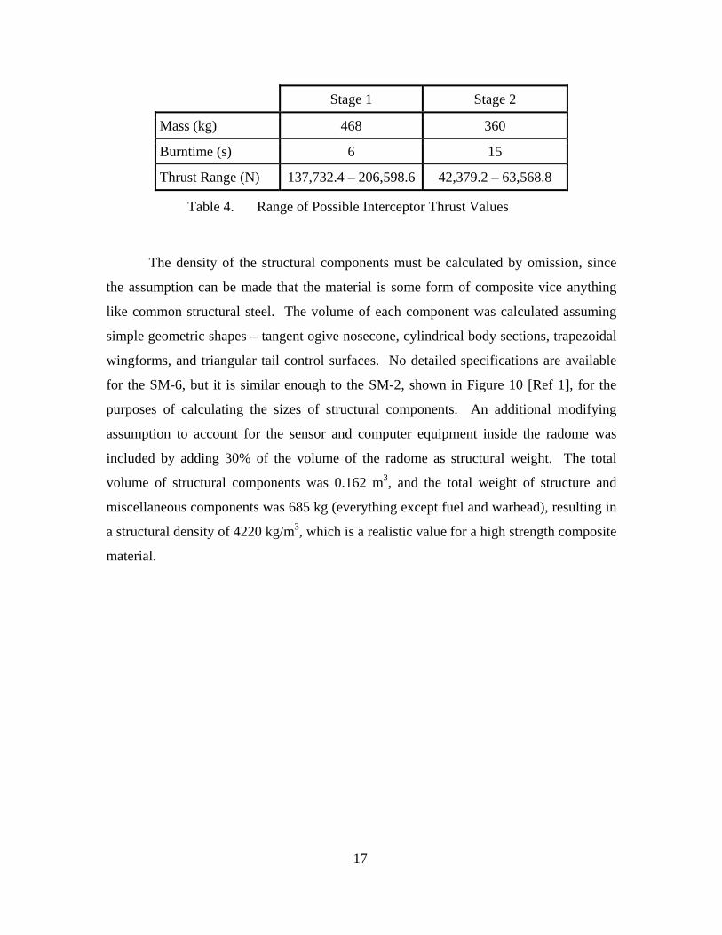
17

Stage 1 Stage 2

Mass (kg) 468 360

Burntime (s) 6 15

Thrust Range (N) 137,732.4 – 206,598.6 42,379.2 – 63,568.8

Table 4. Range of Possible Interceptor Thrust Values

The density of the structural components must be calculated by omission, since

the assumption can be made that the material is some form of composite vice anything

like common structural steel. The volume of each component was calculated assuming

simple geometric shapes – tangent ogive nosecone, cylindrical body sections, trapezoidal

wingforms, and triangular tail control surfaces. No detailed specifications are available

for the SM-6, but it is similar enough to the SM-2, shown in Figure 10 [Ref 1], for the

purposes of calculating the sizes of structural components. An additional modifying

assumption to account for the sensor and computer equipment inside the radome was

included by adding 30% of the volume of the radome as structural weight. The total

volume of structural components was 0.162 m3, and the total weight of structure and

miscellaneous components was 685 kg (everything except fuel and warhead), resulting in

a structural density of 4220 kg/m3, which is a realistic value for a high strength composite

material.

Figure 10. SM-2 Configuration Details (Missile Only)

2. Interceptor Missile Model Program

The 3DOF model presented here is a series of MATLAB functions on a repeating

integration loop, using four function files to accomplish the modeling. (the “3” at the end

of each title refer to the 3DOF model).

1. SMFlight3.m - integrates each time step to determine the current position,

attitude, and aerodynamic forces acting on the rocket/missile;

2. SMParams3.m - determines the mass of the rocket and the surface

reference area;

3. ZLDragC.m - determines the drag coefficient (described in section D);

18

4. STatmos.m – determines the properties of the local atmosphere (described

in section D);

The program SMFlight.m generates the flight plan using the axial velocity, V, the

heading angle, Ψ , and the flight path angle,θ , related through the kinematic equations

[Ref 19]

(2.B.2)

=

=

=

i

i

i

cos cosΨ

cos sinΨ

sin

x V θ

y V θ

z V θ

The three components are the result of the forces acting on the missile, related

through the dynamics equations [Ref 19]

( )( sin )

cos

cos

x

y

z

V g ng nV

g nV

θ

θ θ

θ

= −

= −

Ψ =

(2.B.3)

where is the axial force, is the yaw force, and is the lift force. xn yn zn

Further, the acceleration components are found from the derivatives of equation

(2.B.2).

(2.B.4) 1

2

3

cos cos sin cos cos sin

cos sin sin sin cos cos

sin cos

x V V V

x V V V

x V V

θ θ θ θ

θ θ θ θ

θ θ θ

= Ψ − Ψ −Ψ

= Ψ − Ψ +Ψ

= +

Ψ

Ψ

The axial forces are calculated in the same manner as the axial force of the

ballistic missile, in fact re-using both the STatmos.m and ZLDragC.m functions.

STatmos.m and ZLDragC.m are described in section D of this chapter. The

SMParams.m function uses the same methodology as the BRParams.m function to

calculate the reference surface area and the mass.

19

The thrust is a given set of time-based values based on the known data and the

assumptions, shown in Figure 11. The thrust drops sharply at 6 s and 26 s, again to

represent the staging events.

0 5 10 15 20 250

0.5

1

1.5

2

2.5x 10

5

Time (sec)

Thru

st (N

)

Figure 11. SM-6 Interceptor Thrust Profile

The mass is again a simple function of time (using the function SMParams.m),

shown in Figure 12. The mass drops sharply at 6 seconds and at 26 seconds, again to

represent the staging events.

20

0 5 10 15 20 25400

600

800

1000

1200

1400

1600

1800

Time (sec)

Inte

rcep

tor M

ass

(kg)

Figure 12. SM-6 Interceptor Mass (Boost Phase Only)

The axial thrust force is then the difference between the thrust and drag, and the

axial acceleration is given by

(

xT Dn

mg)−

= (2.B.5)

The remaining two forces, , are returned from the guidance laws and applied by

integrating equations (2.B.3).

,y zn n

3. Results Many of the results are specifically dependant on the guidance law, but several

are relatively independent, such as the Velocity, Acceleration, and generic flight profile.

The Isp of both stages was maximized but still unable to accelerate the SM-6 beyond a

speed of 3,500 m/s. This speed was not detrimental to the simulation and was determined

to be the most accurate value considering all the data. Figure 13 shows the generic 21

Velocity and Acceleration profile produced by the model, which will change slightly with

each run due to the guidance law in effect and specifics of the simulation.

0 10 20 30 40 50-500

0

500

1000

1500

2000

2500

3000

3500

Time (sec)

Figure 13. Interceptor Ve

C. HIGH-FIDELITY MODELING Although the guidance law modeled and d

with a 3DOF models discussed earlier, the follo

fidelity model, such as a Six-Degree-of-Freedom (6

presented here. This model uses the same fundam

but instead of treating the interceptor as a point

velocity, and acceleration, it will also consider atti

step further than the algorithm presented by con

aileron commands.

The higher fidelity modeling was also addr

presented here is a series of MATLAB functions o

22

Likely Intercept Time

60 70 80 90 100

Velocity (m/s)

Acceleration (m/s2)

locity Profile

eveloped in sections III and IV deals

w-on research will require a higher

DOF) model of the interceptor missile

ental algorithm for the guidance law,

mass and considering only position,

tude and orientation. It also goes one

verting acceleration commands into

essed in this study. The 6DOF model

n a repeating integration loop. It uses

23

seven function files to accomplish the modeling, each applying to their respective

simulations (the “6” at the end of each title refer to the 6DOF model). The programs are

very similar, only the control inputs and physical parameters differ.

1. BRInitialize6.m and SMInitialize6.m, which initializes the first step values

based on launch conditions;

2. BRDetail6.m and SMDetail6.m, which describes the rocket/missile

characteristics such as structural thickness, sizes, and fuel weights, etc.

3. BRFlight6.m and SMFlight6.m, which repeats for each time step to

determine the current position, attitude, and aerodynamic forces acting on

the rocket/missile;

4. BRParams6.m and SMParams6.m, which determines the mass of the

rocket/missile and moment of inertia based on time, and several

aerodynamic derivatives;

5. AeroC.m, which interpolates to determine several aerodynamic values

based on angle of attack, altitude, and control surface deflections;

6. ZLDragC.m;

7. STatmos.m;

The output of the model is utilized by the guidance law program, SMGuidance.m,

to determine the necessary inputs to the interceptor missile auto-pilot.

1. Initialization

In order to increase the accuracy of the simulation, the Earth is NOT assumed to

be a perfect, non-rotating spheroid. Based on the World Geographic Survey of 1984, the

following values were used in the program [Ref 14].

Earth's Radius, Re 6,378,137 m

Earth's Semi-Minor Axis, b 6,356,752 m

Earth's Flattening (1/Ellipticity), f 1/298.257223563

Earth's Rotation Rate (ΩzE) 7.292116 e-5 rad/sec

Earth's Gravitational Constant, GM 3.986004418e14 m3/s2

Table 5. WGS-84 Values

A launch point was needed from North Korea, and Pyongyang was chosen

arbitrarily. The coordinates for the launch point (µl, λl) are (40o54' North, 129o34' East).

A suitable US city was needed within the maximum estimated range of the TD-2 missile,

3,500-4,000 km, so Pearl Harbor, at 4,260 km at a bearing of 010o, was selected. The

coordinates for the target point (µt, λt) are 22o03' North by 159o09' West [Ref 5]. The

geocentric launch latitude is found by converting from the geodetic latitude according to

[Ref 8, 14]

2tan (1 ) tans g- fµ µ= (2.C.1)

The coordinates of the launch point were converted from Geodetic into

Rectangular coordinates according to [Ref 14]

2 2 2

2 2, where ,

1 sine

s

s

R a bR eae µ−

=−

= (2.C.2)

and

24

25

s

s

(0) cos

(0) (0) 0(0) sin

x s

y

z s

p Rp p

p R

µ

µ

⎡ ⎤ ⎡ ⎤⎢ ⎥ ⎢ ⎥= =⎢ ⎥ ⎢ ⎥⎢ ⎥ ⎢ ⎥⎣ ⎦ ⎣ ⎦

(2.C.3)

The initial velocity was defined as

0

( ) 00

v o⎡ ⎤⎢ ⎥= ⎢ ⎥⎢ ⎥⎣ ⎦

(2.C.4)

Several different coordinate systems are involved in the flight of the interceptor

missile. The propulsive forces act on the missile at its center of gravity, while the

aerodynamic forces act relative to the movement of the missile with respect to the

atmosphere, and the gravitational forces depend on the position of the missile. In order to

apply all forces equally and appropriately it is necessary to define convenient coordinate

systems for each and then rotate those coordinate systems into a common one. Five

reference frames will be utilized in the model: two geocentric; two geographic; and a

body fixed (subscripted b).

Frame Category Frame of Reference Coordinate System

GeocentricF i , an "inertial frame", non-rotating but translating with Earth's cm

ECI (Earth Centered Inertial), origin at Earth's cm, axes in the equatorial plane and along the spin axis

Geocentric F e , a frame defined by the "rigid" EarthECEF (Earth-centered, Earth-fixed), origin at Earth's cm, axes in the equatorial plane and along the spin axis

GeographicTangent-plane system, a geographic system with its origin on the Earth's surface

GeographicF NED (also F ENU ), a frame translating with the vehicle cm, in which the axes represent fixed directions

Vehicle-carried system, a geographic system with its origin at the vehicle cm

BodyF b , a "body" frame defined by the "rigid" vehicle

Vehicle body-fixed system, origin at the vehicle cm, axes aligned with vehicle reference directions

Table 6. Frame References used in the 6DOF Model (After [Ref 14])

The initial reference frame is Earth Centered Inertial (Fi). This frame includes the

rotation of the earth as a translational motion. The earth's rotation can be removed from

the equation, thereby simplifying the rest of the problem, by rotating the frame about the

z-axis through the angle

0 ELlong Wz tµ λ= − + (2.C.5)

The celestial longitude,λ0, is arbitrary and can be chosen to be zero. The resulting

rotation matrix is [Ref 8,14]

(2.C.6) /

cos( ) sin( ) 0sin( ) cos( ) 0

0 0

E E

e i E E

lLong Wz t lLong Wz tR - lLong Wz t lLong Wz t

+ +⎡ ⎤⎢ ⎥= + +⎢ ⎥⎢ ⎥⎣ ⎦1

where e and i are used to designation ECI and ECEF systems, respectively.

The system must now be rotated into the navigational reference system, normally

designated North-East-Down for the directions that x-y-z point, respectively. However,

and intermediate step is required to rotate from ECEF to Up-East-North first. This is

accomplished by rotating first through the geocentric longitude,

/

cos( ) 0 sin( )0 1 0

sin( ) 0 cos( )u e

latgc latgcR

latgc latgc

⎡ ⎤⎢ ⎥= ⎢ ⎥⎢ ⎥−⎣ ⎦

(2.C.7)

then through the y-axis to point the x-axis North and the z-axis Down,

/

0 0 10 1 01 0 0

n uR⎡ ⎤⎢ ⎥= ⎢ ⎥⎢ ⎥−⎣ ⎦

(2.C.8)

In order to rotate the NED system into the body-fixed system, the initial roll (φ),

pitch (θ), and yaw (ψ) angles must be defined. The initial roll is defined as zero, as the

missile is not rotating about its x-axis on the launch pad. The initial pitch is the elevation

of the launch direction with respect to the horizon. The initial yaw is the initial heading

with respect to north. With these terms defined, the rotation matrices for each variable

are [Ref 22]

26

27

1

1 0 00 cos sin0 sin cos

cos 0 sin0 1 0

sin 0 cos

cos sin 0sin cos 00 0

R

R

R

φ

θ

ψ

φ φφ φ

θ θ

θ θ

ψ ψψ ψ

⎡ ⎤⎢ ⎥= ⎢ ⎥⎢ ⎥−⎣ ⎦

−⎡ ⎤⎢ ⎥= ⎢ ⎥⎢ ⎥⎣ ⎦⎡ ⎤⎢ ⎥= −⎢ ⎥⎢ ⎥⎣ ⎦

(2.C.9)

and the total rotation from NED to body-centered system is

/b nR R R Rφ θ ψ= (2.C.10)

The final complete rotational transformation is the combination of all the rotations

/ / / / /b i b n n u u e e iR R R R R= (2.C.11)

This rotation matrix allows for the computation of several important variables,

notably the angular velocity and the Euler angles which will lead directly to the

Quaternion of this system.

The initial angular velocity is found by transforming the Earth's rotation into the

body system according to [Ref 8]

0 /

00b i

E

b RWz

ω⎡ ⎤⎢ ⎥= ⎢ ⎥⎢ ⎥⎣ ⎦

(2.C.12)

It is often preferable to track the system orientation through the use of the

Quaternion instead of using other methods such as Euler Kinematic Equations or Poisson

Kinematic Equations. The initialization of the Quaternion is derived from the initial

Euler angles. The Euler angles are defined from the rotation matrix Rb/i (a 3x3 Matrix)

( )

/

/

/

/

/

(2,3)1tan(3,3)

1sin (1,3)

(1,2)1tan(1,1)

b iE

b i

E b i

b iE

b i

RR

R

RR

φ

θ

ψ

⎛ ⎞−= ⎜ ⎟⎝ ⎠−= −

⎛ ⎞−= ⎜ ⎟⎝ ⎠

(2.C.13)

The initial Quaternion is calculated from Euler angles [Ref 14]

0

1

2

3

cos( ) cos( )cos( ) sin( )sin( )sin( )2 2 2 2 2 2

sin( )cos( )cos( ) cos( )sin( )sin( )2 2 2 2 2 2

cos( )sin( )cos( ) sin( )cos( )sin( )2 2 2 2 2 2

cos( )cos( )sin( ) sin( )sin( ) cos( )2 2 2 2 2 2

q

q

q

q

φ θ ψ φ θ ψ

φ θ ψ φ θ ψ

φ θ ψ φ θ ψ

φ θ ψ φ θ ψ

= +

= −

= +

= −

(2.C.14)

To check the validity of the Quaternion, the rotation matrix Rb/I can be re-

evaluated [Ref 14]

(2.C.15)

2 2 2 20 1 2 3 1 2 0 3 1 3 0 2

2 2 2 2/ 1 2 0 3 0 1 2 3 2 3 0 1

2 2 2 21 3 0 2 2 3 0 1 0 1 2 3

( ) 2( ) 2(2( ) ( ) 2( )2( ) 2( ) ( )

bb i

q q - q - q q q q q q q - q qR q q - q q q - q q - q q q q q

q q q q q q - q q q - q - q q

⎡ ⎤+ +⎢ ⎥= +⎢ ⎥⎢ ⎥+ +⎣ ⎦

)+

The results should be the same as before.

All the required initial values have now been calculated, and the resulting output

is [Ref 14]

0

00

0

pv

Xwbq

⎡ ⎤⎢ ⎥⎢ ⎥=⎢ ⎥⎢ ⎥⎣ ⎦

(2.C.16)

2. The Flight Program

Once the previous iteration (or the initialization) has been integrated, it is returned

to the program as the current values. The program uses these values to calculate all the 28

descriptive values of the system, apply the corrective time- and position- dependant

factors, and calculate the derivatives for the next iteration.

The angle of attack is -1tan⎛ ⎞⎜ ⎟⎝ ⎠

z

x

vv

and the sideslip angle is -1tan⎛ ⎞⎜ ⎟⎝ ⎠

y

x

vv

. The

program then calculates the necessary control surface deflections to zero the angle of

attack and the sideslip angle, to maintain the alignment of the missile axis and its velocity

vector.

The geocentric latitude is derived from the Cartesian coordinates of the position

[p]

2 2

1tan z

x y

platgcp p

⎛ ⎞− ⎜=

⎜ ⎟+⎝ ⎠

⎟ (2.C.17)

The celestial longitude is derived from rectangular coordinates of [p] with time-

dependant correction factors, subject to a principle value requirement (between -180 and

+180)

1tan yg E

x

plLong Wz t

pλ

⎛ ⎞−= + +⎜ ⎟⎝ ⎠

(2.C.18)

Determining the geodetic coordinates requires an iterative process because the

prime radius of curvature, N, is a function of the geodetic latitude, φ, [Ref 14]

29

12

2 2

2 2

2 2

tan1

Re1 sin

( )cos

( ) iterated while abs( ) < 0.1

zNex y

N h

Ne

x yN h

h N h N h h

h h h

φ

φ

φ

−

⎡ ⎤⎢ ⎥⎢ ⎥=⎢ ⎥⎛ ⎞

+ −⎢ ⎥⎜ ⎟+⎝ ⎠⎣ ⎦

=−

++ =

∆ = + − − ⇐ ∆

= + ∆

(2.C.19)

The ranges and required accuracy of this model prohibit the assumption of a flat

earth with a constant gravitational acceleration vector. The gravitational forces on the

missile are a position dependant correction factor.

2 22

2 222

2 22

[1 1.5 (Re/ ) (1 5sin )] /[1 1.5 (Re/ ) (1 5sin )] /[1 1.5 (Re/ ) (3 5sin )] /

x

y

z

J r pGM J r pr

J r p

ψψψ

⎡ ⎤+ −− ⎢ + −⎢

⎢ ⎥+ −⎣ ⎦

rrr

⎥⎥ (2.C.20)

The atmospheric affects on the missile are dependant on the altitude, which is

derived using the STatmos.m function described in section D.

The missiles speed in m/s is determined by the normalization of the velocity

vector, vb. The missiles Mach number is determined by dividing the speed by the local

Mach number which is determined by the local temperature from the STatmos.m

program ( M RTγ= ).

The moment matrix and missile mass is determined as a function of time and is

based on assumed fuel usage parameters. The missile program calls a separate function,

either SMParams.m, to evaluate the specific descriptive parameters of the ballistic

30

missile. The program assumes a cruciform missile in two stages plus a conical nosecone

section, where only the first stage separates after completion.

The dimensions of the remaining fuel are critical to the purposes of calculating

the center of gravity. For the interceptor, the first stage is active for 6 s while the stage 1

fuel is consumed. The fuel is solid, so the only parameters to change are the length of the

fuel and the inner radius as it is consumed. Once the fuel is totally consumed in stage 1,

the booster separates and stage 2 takes over in a similar manner. Stage 2 lasts for an

additional 20 s. For the rocket, the first stage is active for 125 s while the stage 1 fuel is

consumed. The canister the fuel is contained in is assumed to be a constant size and

diameter, so the only parameter to change is the length of the fuel as it is consumed. The

missile is in a constant forward acceleration, so the fuel is assumed to remain in the rear

of the canister for the purposes of calculating its center of gravity. Thus the center of

gravity of the fuel tends toward the rear of the missile through the flight. Once the fuel is

totally consumed in stage 1, the booster separates and stage 2 takes over in a similar

manner. Stage 2 lasts for 110 seconds.

The center of gravity (CG) is determined by the parallel axis theorem applied

independently to the x, y, and z axes. The missile was separated into five separate pieces:

nosecone, stage 1 structure, stage 2 structure, stage 1 fuel, and stage 2 fuel. Each CG was

separately calculated and then combined. The CG of the individual structural

components was a simple matter of their distance from the nosecone. The center of

gravity of the fuel was then based on the fuel remaining in the canister, referenced to the

base of the missile section. The missile CG is calculated from the locations and masses

of the component sections:

(2.C.21) 1_ 1_ 1_ 1_

2_ 2_ 2_ 2_ nose nose st str st strmissile missile st fuel st fuel

st str st str st fuel st fuel

M CG M CG M CG M CGM CG M CG

= + +

+ +

The moments of inertia for the x, y, and z-axes are calculated using the CG and

the remaining fuel length using a similar methodology of components. For the rocket the

equations are

31

Jxx Jyy = Jzz

Nosecone 2310 noseM r

2223 5

5 4 8⎛ ⎞ ⎛ ⎞+ + −⎜ ⎟⎜ ⎟

⎝ ⎠⎝ ⎠nose nose nose

rM h M CG L

Stage 1

Structure 2 2

0( )2

+stri

M r r 2 2 20 13( ) ( 24)

12⎡ ⎤+ + + −⎣ ⎦

stri st str

M r r L M CG 2

Stage 1

Fuel

2

2fuelM r

2 21(3 ) ( (32 ))

12+ + − −fuel

st fuel fuel

Mr L M CG L

(2.C.22)

Stage 2

Structure 2 2

0( )2

+stri

M r r 2 2 20 23( ) ( 9)

12⎡ ⎤+ + + −⎣ ⎦

stri st str

M r r L M CG 2

Stage 2

Fuel

2

2fuelM r

2 22(3 ) ( (16 ))

12+ + − −fuel

st fuel fuel

Mr L M CG L

The equations for the interceptor are similar.

The J matrix returned is the symmetrical matrix, since the ballistic missile itself is

symmetric:

0 0

00 0

xx

yy

zz

JJ J

J0

⎡ ⎤⎢ ⎥= ⎢ ⎥⎢ ⎥⎣ ⎦

(2.C.23)

The BRParams.m and SMParams.m functions also determine the reference areas

for the control surfaces and missile planform areas using simple equations from Zarchan

[Ref 21]. The function returns the base diameter (dia), reference area (Sref), planform

area (Splan), wing area (Swing), tail area (Stail), nose area (An), body area (Ab), nose center of

pressure (Xcpn), and body center of pressure (Xcpb) according to

32

2

1 1 2 2

1 1 2 2

1 2

40.67

0.5 ( )

0.5 ( )0.670.67

0.67 ( 0.5( ))

ref

plan st st st st nose nose

wing T TT RT

tail T TT RT

n nose nose

cpn nose

b st st st st

nose nose body nose st stcpb

nose body

dS

S L d L d L d

S h C C

S h C CA L d

X L

A L d L dA L A L L L

XA A

π=

= + +

= +

= +==

= +

+ + +=

+

(2.C.24)

The program then calls the function ACoeff.m to determine several necessary

aerodynamic coefficients. The function inputs are angle of attack, altitude, and pitch

control surface deflection. The pitch control surface is specifically included because it

alone varies over the spectrum of possible angles, from -200 to +200, whereas the roll and

yaw derivatives can be assumed to be constant over that range of possible angles. The

pitch deflections therefore require a second interpolation to determine their actual value

at each time step.

Figures 14-20 detail the range of values of the variables returned after

interpolation (all figures after [Ref 7]). Some variables require multiple interpolations,

such as in Figures 14 and 19.

0 5 10 15 20-2

0

2

4

6

CN

Stability Data, Pitch Plane

0 5 10 15 20-4

-2

0

2

4

6

Angle of Attack (deg)

Cm

dP = 0dP = -10dP = -20

Figure 14. Pitch plane stability data

33

0 5 10 15 20-0.25

-0.2

-0.15

-0.1

-0.05

0Yaw Stability Derivatives

CYβ

0 5 10 15 20-0.2

-0.1

0

0.1

0.2


Cnβ

Figure 15. Yaw stability and control derivatives

0 5 10 15 200.04

0.06

0.08

0.1

0.12


Cl δ

R

Roll Control Derivative

Figure 16. Roll control derivatives

34

0 5 10 15 20

-0.04

-0.02

0

Roll Control Coupling Derivatives

CYδR

0 5 10 15 200

0.04

0.08

0.12

0.16


CnδR

Figure 17. Roll control Coupling Derivatives

0 5 10 15 20

-0.03

-0.02

-0.01

0

Yaw Control Derivatives

Cl δ

Y

0 5 10 15 200

0.05

0.1

CYδY

0 5 10 15 20-0.3

-0.2

-0.1

0


CnδY

Figure 18. Yaw control Derivatives

35

0 5 10 15 200

0.1

0.2

0.3

Angle of Attack (deg)C

l β

Effect of Pitch Control on Roll Stability

dP = 0dP = -10

Figure 19. Pitch control effects on roll stability

0 10 20 30 40 50 60 70 80 900.162

0.164

0.166

0.168Pitch Control Derivatives/Aeroelastic Missile

CNδP

0 10 20 30 40 50 60 70 80 900.06

0.07

0.08

0.09

0.1

0.11

0.12

Altitude (km)

CmδP

Figure 20. Pitch control derivatives

The returned values are combined together to calculate the force and moment

coefficients [Ref 7]

36

37

Y

l

n

R

R

R

( , , , , )

( , )

( , , , , )

( , )

( , , , , )

Y R

P

Y R

P

Y R

Y Y Y

N N N

l l l

m m m

n n n

C P Y R C C Y C

C P C C P

C P Y R C C Y C

C P C C P

C P Y R C C Y C

β δ δ

α δ

β δ δ

α δ

β δ δ

α β δ δ δ β δ δ

α δ α δ


α δ α δ


= + +

= +

= + +

= +

= + +

(2.C.25)

The program calls the function ZLDragC.m to determine the value of the drag

coefficient. The Thrust is determined exactly as before, by simple time dependence. The

total force on the body of the missile from all lift, drag, thrust, and aerodynamic forces is

then [Ref 22]

2sin

[ ] 02

0cos

ro ref Nx xb

y ro ref

z ro ref N z

q S Cf VThrustf f q S V

f q S C V

αρ

α

⎡ ⎤−⎡ ⎤ ⎡ ⎤⎡ ⎤⎢ ⎥⎢ ⎥ ⎢ ⎥⎢ ⎥= = + −⎢ ⎥⎢ ⎥ ⎢ ⎥⎢ ⎥⎢ ⎥⎢ ⎥ ⎢ ⎥⎢ ⎥⎣ ⎦⎣ ⎦ ⎣ ⎦⎣ ⎦

y (2.C.26)

The torque experienced by the missile from all moment forces is [Ref 7]

l

ro ref m

n

CT q S d C

C

⎡ ⎤⎢ ⎥= ⎢ ⎥⎢ ⎥⎣ ⎦

(2.C.27)

The inertial-body centered rotation matrix is determined using the quaternion

2 2 2 20 1 2 3 1 2 0 3 1 3 0 2

2 2 2 2/ 1 2 0 3 0 1 2 3 2 3 0 1

2 2 2 21 3 0 2 2 3 0 1 0 1 2 3

( ) 2( ) 2(2( ) ( ) 2( )2( ) 2( ) ( )

bb i

q q - q - q q q q q q q - q qR q q - q q q - q q - q q q q q

q q q q q q - q q q - q - q q=

+ + )⎡ ⎤⎢ ⎥+ +⎢ ⎥⎢ ⎥+ +⎣ ⎦

(2.C.28)

Also, as before, the ECI-inertial rotation matrix is determined as

(2.C.29) /

cos( ) sin( ) 0sin( ) cos( ) 0

0 0

E E

e i E E

lLong Wz t lLong Wz tR - lLong Wz t lLong Wz t

+ +⎡ ⎤⎢ ⎥= + +⎢ ⎥⎢ ⎥⎣ ⎦1

)

The total rotation matrix is then

(2.C.30) / / / /( Tb n n e e i i bR R R R=

The Euler angles with respect to the ECEF system are [Ref 8]

( )

/

/

/

/

/

(2,3)1tan(3,3)

1sin (1,3)

(1,2)1tan(1,1)

b n

b n

b n

b n

b n

RR

R

RR

φ

θ

ψ

⎛ ⎞−= ⎜ ⎟⎝ ⎠

−= −

⎛ ⎞−= ⎜ ⎟⎝ ⎠

(2.C.31)

The quaternion rotation matrix is calculated is [Ref 14]

/

00

00

bb i

-P -Q -RP R -Q -R PR Q -P

Q⎡ ⎤⎢ ⎥⎢ ⎥Ω =⎢ ⎥⎢ ⎥⎣ ⎦

(2.C.32)

The centripetal acceleration due to the rotation of the missile and its velocity is

the vector product [Ref 14]

b/i

00

0

-R QR-Q P

P⎡ ⎤⎢ ⎥Ω = ⎢ ⎥⎢ ⎥⎣ ⎦

(2.C.33)

The centripetal acceleration due to the Earth's angular velocity and the rotation in

the ECI frame is the vector triple product [Ref 14]

2

2/

0 00 0

0 0 0

Eie i E

-WzWz⎡ ⎤⎢ ⎥Ω = ⎢ ⎥⎢ ⎥⎣ ⎦

(2.C.34)

All values, coefficient, and matrices have been determined. The full state

parameters can be calculated as [Ref 14]

/ / /

/ , / / / / / / /

1/ , /

/ / /

* *1 *( * ) ( )*

( ) *( )1 *2

i iCM O b i b e i i

b b b i i i b T bCM e A T b i e i CM O b i b i e i b i CM e

b b b - b b b bb i A T b i

bb i b i b i

p R v p

v F R G - p - R R vmJ M - J

q q

ω ω

= +Ω

= + Ω Ω + Ω

= Ω

= Ω

/

(2.C.35)

38

3. Results In order to fully visualize the geometry of the intercept, an animation function

was developed that shows side-by-side the orientation of the target and the interceptor. A

screen shot of the plot is shown in Figure 21. The animation shows the stage changes of

the missile as well, dropping the used stages at the appropriate moment.

East (yLTP)

Up

(-zLT

P)

Ballistic Missile Attitude

Frame 2 out of 146Time 0.00 sec

East (yLTP)

Up

(-zLT

P)

Interceptor Attitude

Speed Speed

Figure 21. 6DOF Orientation Animation

D. COMMON FUNCTIONS Two functions were common to all the models, ZLDragC.m and STatmos.m.

1. ZLDragC.m The drag on the missile is dependant on two conditions, the Mach number and

whether the missile is in the boost or glide phase. The phase of the missile is easily

determinable from the time.

39

The reason the values differ is the presence or absence of the base drag. When

the rocket is under power, the thrust pressure is balanced to atmospheric, so there are no

parasitic drag effects from the tail section. After the engine shuts down, there is no

longer any pressure generated, so the sharp end of the tail section generates a drag effect.

Parasitic drag from the rest of the missile is relatively constant in both phases of the

missile flight.

There is a sharp increase in the drag effects at Mach one, after which the drag

drops considerably [Ref 8]. Figure 22 shows the effect of speed on the drag coefficient.

0 1 2 3 4 5 60.05

0.1

0.15

0.2

0.25

0.3

0.35

0.4

0.45

0.5

Mach Number

Zer

o L

ift

Dra

g C

oef

fici

ent

Drag Coefficient by Mach Number and Boost Phase

Boost PhaseGlide Phase

Figure 22. Drag Coefficient by Mach Number and Flight Phase

The drag force is then calculated from

2

2DVDrag C ρ

= (2.D.1)

and the atmospheric dynamic pressure is calculated from

2

2roVq ρ

= (2.D.2)

2. STatmos.m Many of the atmospheric affects on the missile are dependant on the altitude. The

missile program calls a separate script, STAtmos.m, to determine the density, pressure,

and temperature of the local atmosphere. The script is based on the 1976 standard

40

atmospheric survey, and includes values up to 86 km in a tabular format. Figures 23-25

show the details of the values returned.

180 200 220 240 260 280 3000

10

20

30

40

50

60

70

80

90

Temperature (K)

Alt

itu

de

(km

)

Atmospheric Temperature Variation by Altitude

Figure 23. Atmospheric Temperature Variation by Altitude

0 0.2 0.4 0.6 0.8 1 1.2 1.40

10

20

30

40

50

60

70

80

90

Density (kg/m3)

Alt

itu

de

(km

)

Atmospheric Density Variation by Altitude

Figure 24. Atmospheric Density by Altitude

41

0 10 20 30 40 50 60 70 80 900

10

20

30

40

50

60

70

80

90

Pressure (kPa)

Alt

itu

de

(km

)

Atmospheric Pressure Variation by Altitude

Figure 25. Atmospheric Pressure Variation by Altitude

42

43

III. EXISTING GUIDANCE LAWS

There are a wide variety of guidance laws available for missile guidance processing.

Many of them are not acceptable for this application such as Beam Rider and Pure Pursuit, while

others are acceptable though not optimal such as Proportional Navigation and its variants.

A. UNACCEPTABLE GUIDANCE LAWS

1. Beam Rider

Beam Rider (also called Command Line-of-Sight) is among the simplest forms of

command guidance. The missile simply flies along a tracker beam that is continuously pointed at

the target. In other words, the inertial velocity vector is continuously pointed at the target. The

beam and the missile generally originate from the same position, but not always. The guidance

commands are proportional to the angular error between the missile and the beam, and if the

missile remains exactly on the beam it will hit the target. There is no consideration for the

capabilities of the target, and the missile is not directed to orient itself to lead the target in order

to anticipate its movements. The missile therefore requires much greater maneuvering

capabilities in the moments just prior to interception. This form of guidance law also assumes

that the shooter will have a direct line of sight for the entire engagement, and that the diffraction

of the beam will be negligible, which is obviously not true over the distances required for a BPI.

[Ref 2]

2. Pure Pursuit

Pure Pursuit overcomes this limitation by having the missile supply the targeting data

instead of a third-party observer. This is, in effect, Beam Rider Guidance where the beam is

generated onboard the missile. As before, the missile only follows the beam and the guidance

commands are proportional to the angular error between the missile and the line of sight to the

target. This overcomes the diffraction of the beam, but still does not command the missile to

orient itself to lead the target. It thus requires similarly large maneuvering capabilities to

complete the interception.

Both of these guidance laws are severely limited in their effectiveness, are used

only at short range against non-maneuvering or relatively slow targets, and require

44

significant interceptor capabilities relative to the target. This is not an accurate

description of the requirements for a BPI, and both laws are therefore discounted for use

here. [Ref 2]

B. LESS THAN OPTIMAL GUIDANCE LAWS

1. True Proportional Navigation

Another family of guidance laws involves Proportional Navigation (PN) and its

derivatives. Of the three basic guidance laws, proportional navigation is the most versatile, and

therefore most frequently implemented, making it the guidance law of choice in nearly all

modern guided missiles. In proportional navigation the rate of change of the missile heading is

proportional to the rate of rotation of the line-of-sight (LOS) from the missile to the target. The

guidance system points the differential velocity vector at the target [Ref 2]

In order for interception to occur, the heading angle and the LOS angle, λ, must remain

constant. If the target increases speed, then λ will increase and the interceptor must increase its

heading Ψ to compensate. Thus it is apparent that they must be proportional to each other, or

more accurately, the rate of change of each must be proportional, [Ref 21]

NλΨ = (3.B.1)

where N is the proportionality constant, which determines the amount of target lead by the

interceptor (usually 3-5 depending on the interceptor’s maneuvering capabilities). The

interceptor maneuvers until , at which point 0λ = 0Ψ = and no further maneuvers take place

until intercept.

The missile seeker measures the LOS rate and the PN guidance law converts that into an

acceleration command by the guidance computer. Using the fact that the acceleration normal to

the velocity vector of the interceptor is

Da V= Ψ (3.B.2)

which can be correlated to the LOS rate to develop the steering command for the guidance

computer

Da NV λ= (3.B.3)

The same method applies to the extension of this law into three dimensions.

45

Using angular velocity vectors between the target and interceptor, Zipfel [Ref 22]

develops a three dimensional PN guidance law as

D OEva NV u g= Ω − (3.B.4)

where is the cross product of the LOS frame with the Earth and the velocity vector with VEΩ

respect to the Earth, is the unit vector of vu DV , and g is the added gravity bias.

2. Compensated Proportional Navigation

True PN is rarely implemented in this simple form, however. The thrust generated by

the interceptors motor creates a parasitic acceleration in the LOS angle that must be

compensated for in the autopilot command or intercept errors will occur. Such a guidance law is

termed “compensated”. The missile acceleration is projected onto the LOS plane by

[ ] [ ]LOS wLOSm wa R= ma (3.B.5)

and subtracted from the PN command in equation (3.B.4) to obtain the augmented command

[Ref 22]

(3.B.6) [ ] [ ] [ ]w w wD OE LOS wv w m na NV u R a R g⎡ ⎤= Ω − −⎣ ⎦

n

where the rotation matrix LOSw R of the LOS coordinates with respect to the wind frame is defined

by the azimuth and elevation angles from the LOS vector.

3. Augmented Proportional Navigation Zarchan details one further variation of PN, termed Augmented Proportional Navigation

which includes an extra term to account for the acceleration of the target [Ref 21].

2

D OEv T

Na NV u n g= Ω + − (3.B.7)

where nT is the acceleration of the target. However, a detailed knowledge of the target’s

acceleration requires an advanced Kalman filter, such as an Extended Kalman Filter or an

Alpha-Beta-Gamma Filter, which are not sufficiently accurate [Ref 13] and is not feasible

to be implemented onboard an interceptor as small as the Standard Missile. Additionally,

application of the acceleration would require exact knowledge of the target’s staging

events where the acceleration value changes radically.

C. KEY FATAL CHARACTERISTICS There are three fatal characteristics of these guidance laws which can preclude the

interceptor from impacting the target: the dynamics of the missile controls system, the

lack of knowledge of the end-game environment, and the inability to control the intercept

geometry.

1. Control System Time Constant

If the dynamics of the seeker, noise filter and flight control system are neglected,

a perfect or zero-lag guidance system is achieved and the missile will always hit the

target if it is tracked correctly. In reality, guidance commands can not be implemented

instantaneously and there will be lags or dynamics within the guidance system. In

missile systems, the dominant portion of the total system time constant is usually

associated with the flight control system actuators such as the tail fin control surfaces

[Ref 21]. Such time lags are generally represented by a time constant

11

L

c

nn s

=+ T

(3.B.8)

where is the achieved missile acceleration, is the commanded missile acceleration,

and T is the flight control system time constant. Zarchan has shown that even a very

good 1-second time constant can have a considerable impact on the miss distance [Ref

21]. A system with a small guidance system time constant has the potential for having

very small miss distances. However, technology issues limit how small the guidance

system time constant can be. Thus all systems that utilize current target information in a

homing guidance loop with a feedback control system will have some miss distance due

to the flight control system time constant.

Ln cn

46

47

2. End-game Environment The lack of knowledge of end-game environment is also a major problem.

Missiles use fuel for a fraction of the flight to generate a set amount of thrust and speed,

after which the missile must glide to the target under a constant drag- and gravity-induced

deceleration. The amount of available maneuver capability depends on the missile speed

and altitude of engagement – higher speeds and lower engagement altitudes work to

increase the missile capability [Ref 20]. Therefore trajectories should be flown to

maximize the missile velocity and minimize the intercept altitude so that there is

sufficient acceleration left to intercept the target.

Yet the above guidance laws do not consider the end-game prior to achieving it.

The effect is to guide the missile along the most direct path and hope that the interception

will take place under atmospheric conditions that are acceptable to the interceptor and to

try to minimize the acceleration at each moment with the hope that there will be enough

capability remaining to complete the end-game. The assumption that target maneuvers

will be sufficiently small enough that the missile will have enough capability to counter

them is usually accurate; however, the immense accelerations involved in a BPI makes

active management of the missile’s acceleration critical to ensuring the end-game is

successful.

3. Controlling the Interception Geometry The interception geometry of any engagement under the above guidance laws is a

result of the relative speeds of the missile and target, the launch geometry, and the

maneuvers involved. The above guidance laws have no control over any of these aspects,

though this geometry is critical to ensuring the interceptor is capable of destroying the

ICBM. An overtaking intercept (the interceptor approaches the target from the rear) is

significantly less desirable than a head-on or a right-angle intercept.

Only if the intercept geometry is controllable can it be expected to conform to a

pre-determined setup. Since none of these guidance laws can control the geometry, they

are not capable of maximizing the kinetic energy transfer via the intercept geometry.

48


IV. PROPOSED ALGORITHM

A method that overcomes fatal characteristics of modern guidance laws is the key

driving factor in the development of this advanced guidance law. The guidance law will

determine the near-optimal flight path from the interceptor position to a predicted target

position for the interceptor to follow to intercept, and then derive the set of control

commands necessary to execute that flight. This section will describe a method for

deriving that trajectory using calculus of variations based on three cues: high-order

polynomials as a reference function for the flight path, a preset thrust history as one of

the controls, and a few optimization parameters. The trajectory optimization problem is

then converted into a nonlinear programming problem and solved numerically.

A. PROBLEM STATEMENT Among all admissible trajectories,

1 2

0

( ) ( ), ( ), , ( )

( ) , ,

Tr

r rf

z t z t z t z t S

S z t Z E t t t

= ∈

⎡ ⎤= ∈ ⊂ ∈ ⎣ ⎦

… (4.A.1)

that satisfies:

1. The system of differential equations (dynamic constraints):

( , , , ), 1,i i t z u a i rfz = = (4.A.2)

where the vector of controls is

1 2( ) ( ), ( ), , ( ) , , Т mmu t u t u t u t m r u U E= <… m∈ ⊂

⊂

and the vector of

missile parameters is 1 2( , , , ), p ppa a a a a A E= ∈… ;

2. The initial conditions:

0 0 0 0( ) , r rz t S S z Z E∈ = ∈ ⊂ (4.A.3)

0 0 0 0( ) , m mu t R R u U E∈ = ∈ ⊂ (4.A.4)

and the final conditions:

49

( ) ( )( ) , ; 0, 1,r rf f f f j fz t S S z Z E G z t j l∈ = ∈ ⊂ = = (4.A.5)

( ) , m mf f f fu t R R u U E∈ = ∈ ⊂ (4.A.6)

3. The constraints imposed on the state space

1 2( , ) ( , ), ( , ),..., ( , ) 0Т

t z t z t z t zµη η η η= ≥ (4.A.7)

on the controls

(4.A.8) 1 2( , , ) ( , , ), ( , , ),..., ( , , ) 0Тt z u t z u t z u t z uνξ ξ ξ ξ= ≥

and on the controls derivatives

1 2( , , ) ( , , ), ( , , ),..., ( , , ) 0Т

t u u t u u t u u t u uσπ π π π= ≥ (4.A.9)

Find the optimal trajectory, ( )optz t , that minimizes the integral function

0

0( , ) ( , , )ft

ft

J K x x L t z u dt= + ∫ (4.A.10)

and the corresponding optimal controls, ( )optu t , where K, L are defined functions.

B. CALCULUS OF VARIATIONS

Calculus of variations deals with functions of functions, termed functionals,

instead of functions of some variable or variables as in ordinary calculus. Specific

interest is in the extremals of these functionals - those making the functional attain a

maximum or minimum value [Ref 15]. There are two broad categorizations of methods

to solve these problems, indirect methods and direct methods.

Indirect methods resolve the problem into a differential equation, usually via the

difference of a series of equations of motion and thus solve the general theory of partial

differential equations. This method does not assume anything about the solution, leading

to a very complete and perfectly precise answer; however, one must integrate the

resultant equation to derive the extremals. The precision greatly increases the

computational complexity, and therefore the time required to solve, for negligible gain in

50

optimality. Further, these differential equations are difficult to integrate except in the

simplest of cases, and nearly impossible to program [Ref 19]. This approach is further

complicated by the need to solve the problem in a specified fixed region instead of in the

small neighborhood of some point. These difficulties can be overcome by using direct

methods, which do not reduce the variational problems to ones involving differential

equations.

The fundamental idea of direct methods is to consider a variational problem as a

limit problem of the extreme of a function of a finite number of variables that can be

solved by numerical methods. Two basic direct methods are the Rayleigh-Ritz and

Galerkin methods, which assume the solution to be an unknown function but of a certain

form containing a set of unknown coefficients (themselves functions of the boundary

conditions), which are then found by minimization. The practical result is that the

problem has been reduced from calculus to algebra, but at the cost of a significant

increase in the number of simultaneous equations to be solved. It is for this reason that

little work was done in this field until the advent of computer technology. The possible

solution set is restricted to a smaller space than the original equation because of the initial

assumption regarding the solution, but the resultant problem can be programmed and

quickly solved using computers; however, the solutions are only an approximation of the

original solution. Therefore these solutions can only be regarded as near-optimal

solutions.

Professor Taranenko [Ref 19] first applied the ideas of direct methods and the

combination of Ritz and Galerkin methods to the problems of flight dynamics by

identifying a reference function for the flight vehicle’s motion and velocity

00 0

0

( ) ( ), 1i i if i if

x x x x i , 4τ τ ττ τ−

= + − +Φ =−

(2.1)

where are the Cartesian coordinates for the flight path, is the velocity, and 1 2 3, , ,x x x 4x

( )i τΦ is a continuous, unequivocal, differentiable function satisfying the boundary

conditions 0( ) ( ) 0i i fτ τΦ = Φ ≡ . Any function that satisfies those conditions would be

acceptable for use. Taranenko called τ a virtual arc. It is this critical variable that allows

51

the separation of the spatial trajectory from the velocity and thus optimizes one or the

other, or both independently. The specific task determines the appropriate choice of τ ,

but in general any continuous, monatomic function is acceptable: time, path, energy, etc.

The remaining state parameters and flight controls are then determined by solving the

inverse problem of flight dynamics. Rather than starting with the control time histories

and integrating them to determine the flight path, this method starts with a flight path and

determines the control time histories necessary to create it.

In order to implement a solution to this problem that can be solved in real time, a

further restriction must be made. The continuous problem must be discretized to reduce

the infinite variational problem to one of optimization of few parameters at numerous

sampling points. This allows for the optimization of the planar trajectory of the missile at

several points along the path by presetting the state variables and one of the controls’

time histories, and then solving the inverse flight dynamics problem.

These methods have all previously been used for off-line optimization of

trajectories, but none has yet been applied to the real-time onboard optimization of a

missile flight path. Yakimenko detailed a method called a Direct Method for Rapid

Prototyping, which he applied to short term spatial trajectories of aircraft maneuvers

using fixed boundary points [Ref 19]. The developed program presented here uses similar

numerical method to provide a near-optimal spatial trajectory that is completely defined

by a few optimization parameters, but as will be discussed shortly, has fluid final

boundary conditions.

Though the method artificially limits the possible trajectory variations, it does

guarantee the following [Ref 19]:

1. The boundary conditions are satisfied a priori,

2. The control commands are physically realizable and smooth,

3. Only a few variable parameters are used, thus ensuring that the iterative

process converges well,

4. The near-optimal solution is very close to the optimal one.

52

A simple two dimensional variation program of a similar 7th order system will

demonstrate how the direct method varies the flight path according to the boundary

conditions. The boundary conditions are

53

1== −

10 20 1 2

10 20 1 2

10 20 1 2

10 20 1 2

0 0 10.2 1 0.1 10.1 0.1 0.1 0.1var 0.1 0.1 0.1

f f

f f

f f

f f

x x x xx x x xx x x x

x''' x''' x x'''

= = =′ ′ ′ ′= = =′′ ′′ ′′ ′′= = = =

′′′= = = =

where the third derivative of the initial condition has been set to vary according to 1x

10 0.4; 0.1;0.2;0.5x''' = − −

and the length of the virtual arc varies according to

1, 2,...,10fτ =

The resulting set of paths is shown in Figure 26 and the first derivative of the path is

shown in Figure 27. It is important to note that the first derivative is not “velocity” but is

instead the “rate of change of the path”. It is proportional but not equal to velocity,

specifically because of the virtual variable τ as discussed previously. Each line

represents a different choice of fτ , showing that by varying that value the length of the

path can change drastically. The algorithm developed here will use this technique to

derive the optimal flight path.

0 0.5 1 1.5 20

2

4

6

τf=var

d3x/dτ3|0=-0.4

0 0.5 1 1.5 20

2

4

6

τf=var

d3x/dτ3|0=-0.1

0 0.5 1 1.5 20

2

4

6

x1

x 2

τf=var

d3x/dτ3|0=0.2

0 0.5 1 1.5 20

2

4

6

τf=var

d3x/dτ3|0=0.5

Figure 26. Variation of Path with fτ and 10x′′′ (after [Ref 18])

0 2 4 6 8 100

1

2

3

4

τf=var

d3x/dτ3|0=-0.4

0 2 4 6 8 100

1

2

3

4

τf=var

d3x/dτ3|0=-0.1

0 2 4 6 8 100

1

2

3

4

τ

√(x/ 12 +x

/ 22 )

τf=var

d3x/dτ3|0=0.2

0 2 4 6 8 100

1

2

3

4

τf=var

d3x/dτ3|0=0.5

Figure 27. Variation of First Derivative of Path with fτ and 10x′′′

54

C. PROGRAM DEVELOPMENT

1. Boundary Conditions

55

Using equations (3.2) and (3.3), in addition to the controls , it is possible

to construct the vector of state variables

, ,x y zn n n

1 2 3, , , , , Tz x x x V θ= Ψ and the vector of controls

. The model for thrust, drag, and missile characteristics is the same as

previously used in Chapter 3.

, , Tx y zu n n n=

The beginning assumption is that the following data is known by the interceptor’s

onboard computer:

Interceptor Target

Body Frame

1 0 10

2 0 20

3 0 30

0 0 10

0 0 20 10

0 0 30 20

0 0

0 0

( )( )( )( )( )( )( )( )

y y

z z

x t xx t xx t x

30

V xt x xt x x

n xn

θ θ

====

Ψ = Ψ===

V t

n tn t

1 1

2 2

3 3

1

2

3

( )( )( )( )( )( )

f f

f f

f f

f f f

f f f

f f f

x t xx t xx t xV t V x

t xt xθ θ

====

Ψ = Ψ=

Earth Centered Inertial

1 2 3( ), ( ), ( )SM SM SMx t x t x t

1 2 3( ), ( ), ( )SM SM SMx t x t x t

1 2 3( ), ( ), ( )SM SM SMx t x t x t

1 2 2( ), ( ), ( )BR BR BRx t x t x t

1 2 3( ), ( ), ( )BR BR BRx t x t x t

Table 7. Interceptor Known Data

The target data will be used to determine the final boundary conditions of the

interceptor missile according to the time until intercept, t∆ :

Position:

1 10 10

2 20 20

3 20 20

SM BR BRf

SM BR BRf

SM BR BRf

x x x t

x x x t

x x x t

= + ∆

= + ∆

= + ∆

(4.C.1)

Heading and Flight Path Angle:

32 2

1 2

2

1

, where arctg2

, where arctg

BRSM BR BRf f f BR BR

BRSM BR BRf f f BR

xx x

xx

πθ θ θ

ψ ψ ψ

= + =+

= =

(4.C.2)

which, when combined with reasonable estimates of the final values of the velocity, V,

and the time rate of change of velocity,V , heading ( 0Ψ = ), and flight path angle

( ), yields the final conditions: 0θ =

1

2

3

cos cos

cos sin

sin

SMf f f

SM

f

f f f

SMf f f

x V

x V

x Vf

θ ψ

θ ψ

θ

=

=

=

(4.C.3)

and

1

2

3

cos cos sin cos cos sin

cos sin sin sin cos cos

sin cos

SMf f f f f f f f f f f

SM

f

f f f f f f f f f f f

SMf f f f f f

x V V V

x V V V

x V V

θ θ θ θ

θ θ θ θ

θ θ θ

= Ψ − Ψ −Ψ

= Ψ − Ψ +Ψ

= +f

Ψ

Ψ (4.C.4)

In order to ensure a smooth flight path at the initial and final points, an additional

constraint of

1 1

2 2

3 3

0

0

0

SM SMi f

SM SMi f

SM SMi f

x x

x x

x x

= =

= =

= =

(4.C.5)

will be imposed on the system at the initial and final conditions. This will have the

practical result of limiting the initial and final controls on the system to smooth

maneuvers, thus avoiding any tendancy to conduct a “flair maneuver” at the last second.

In current air-to-air engagements, the kill capability of the warhead can be greatly

56

improved by a last minute change in the orientation of the missile, a rapid jerk of the

attitude from the flight path to an optimal angle, which is termed a “flair maneuver”.

This focuses the blast effects toward the target and is of great usefulness when it is the

warhead damage that kills the target; but in this situation it is the kinetic energy of the

missile impact that kills the target. A flair maneuver would only dissipate much of that

energy, possibly all of it, in order to achieve the algorithm’s desired impact angle and

render the developed flight path useless for the mission. Similarly, an immediate and

large maneuver at the start of the flight path would only dissipate the energy. Such

maneuvers are discarded by these beginning and ending boundary conditions.

2. Separating and Recombining Space and Time As discussed previously, in order to independently optimize the spatial trajectory

and the velocity, the reference function will be derived as a function of τ . The boundary

conditions cannot, therefore, be defined as functions of time derivatives as in equations

(4.C.3) – (4.C.5). A connection between the spatial and time domains must therefore be

introduced,λ , which is defined as

( ) ddtτλ τ = (4.C.6)

and is termed the virtual speed [Ref 19]. This allows for the independent variation of the

speed profile along the same paths according to any other convenient reference. In this

case the known thrust profile, , will be utilized by integrating the third equation of

(2.B.3) and applying the virtual speed

xn

( sin( ) ( sin )

( )x

xg ndV g n

dt)θττ θ

λ τ−′ = − = (4.C.7)

Further use of the virtual speed allows the recalculation of the initial and final boundary

conditions, transforming them from the time frame to the spatial frame. For this, the

obvious relations

57

2

( ) ( ) ( )

( ( ) ( ))( ) 1, 2,3

ii i

ii i i

dx dx xd dtd x dx x x

d dti

ττ τ λ ττ

τ λ τ ττ λ λτ

′= =

′′′ ′= = + =

(4.C.8)

which when rearranged defines the first and a second derivative of the missile

coordinates as

[ ]1 2 1, 2,3i i i i ix x x x x iλ λ λ− −′ ′′ ′= = − = (4.C.9)

Using the values of λ and λ′ defined as

10 0 0 0 0, , 1

f f f fV V V V Vλ λ λ λ fV− −′= = = =′ (4.C.10)

3. Reference Trajectory

The knowledge of the initial and final position plus the initial and final conditions

of the first and second time derivates allows for the construction of a 7th-order

polynomial (the maximum orders of the time derivatives of the missile coordinates at the

initial and final points plus one) to describe the reference function of the aircraft

coordinates . The following are introduced as the reference functions [Ref

19]:

( 1,2,3)ix i =

5

0

15

1

52

2

53

3

(max(1, 2))!( )!

(max(1, 2))!( )( 1)!

( )

( ) ( 2)

k

i ikk

k

i ikk

ki ik

k

ki ik

k

kx akkx a

k

x a

x k a

ττ

ττ

τ τ

τ τ

=

−

=

−

=

−

=

−=

−′ =−

′′ =

′′′ = −

∑

∑

∑

∑

(4.C.11)

Or written another way,

58

2 3 43 4 5 6 7

2 3 4 52 3 4 5 6 7

2 3 4 5 61 2 3 4 5 6 7

2 3 4 50 1 2 3 4 5

( )1 1 1 1 ( ) 2 3 4 51 1 1 1 1 ( )2 6 12 20 301 1 1 1 1 ( )2 6 24 60 120

i i i i i i

i i i i i i i

i i i i i i i i

i i i i i i i i

x"' a a a a a

x" a a a a a a

x' a a a a a a a

x a a a a a a a

τ τ τ τ τ

τ τ τ τ τ τ

τ τ τ τ τ τ τ

τ τ τ τ τ τ

= + + + +

= + + + + +

= + + + + + +

= + + + + + + 6 76 7

1210 iaτ τ+

(4.C.12)

The coefficients can be determined by solving the equations simultaneously,

0

1

2

32 3 4 5 6 71 1 1 1 1 1

2 6 24 60 120 210 42 3 4 5 61 1 1 1 1

2 6 12 20 30 52 3 4 51 1 1 1

2 3 4 5 62 3 4

7

1 0 0 0 0 0 0 00 1 0 0 0 0 0 00 0 1 0 0 0 0 00 0 0 1 0 0 0 010 10 0 10 0 0 1

i

i

i

i

f f f f f f f i

f f f f f f i

f f f f f i

f f f f i

aaaaaaaa

τ τ τ τ τ τ ττ τ τ τ τ τ

τ τ τ τ ττ τ τ τ

⎛ ⎞⎛⎜ ⎟⎜⎜ ⎟⎜⎜ ⎟⎜⎜ ⎟⎜⎜ ⎟⎜⎜ ⎟⎜ ⎟⎜ ⎟⎜ ⎟⎜ ⎟⎜ ⎟⎝⎝ ⎠

0

0

0

0

i

i

i

i

if

if

if

if

xxx

x'''xxx

x'''

⎛ ⎞⎞⎜ ⎟⎟ ′⎜ ⎟⎟⎜ ⎟⎟ ′′⎜ ⎟⎟⎜⎟ = ⎜⎜ ⎟⎜ ⎟⎜ ⎟

′⎜ ⎟⎜ ⎟⎜ ⎟⎜ ⎟ ′′⎜ ⎟⎜ ⎟⎜ ⎟ ⎜ ⎟⎠ ⎝ ⎠

⎟⎟ (4.C.13)

Finally, by substituting the corresponding values of 0 0 0, , ( 1,2,3)i i ix x x i′ ′′ = for

0 0τ = , and for , , ( 1, 2,3)if if ifx x x i′ ′′ = fτ τ= (where fτ is the first optimization parameter,

the virtual arc), results in a set of 24 linear algebraic equations for 21 unknown

coefficients ( 1,2,3, 0,1,..,7)ika i k= =

0 0 1 0 2 0 3

0 0 0 04 2 3 4

0 05 2

4 16 60 120 360 480 840 840

30 60 420 600

i i i i i i i

if i if i if i if ii

f f f f

if i if ii

f

a x a x a x a xx x x x x x x x

a

x x x xa

τ τ τ τ

τ τ

′ ′′ ′′′= = = =′′′ ′′′ ′′ ′′ ′ ′− + − − − −

= + + +

′′′ ′′′ ′′ ′′+ − += + 0 0

3 4 5

0 0 06 3 4 5 6

0 0 07 4 5 6

2340 2700 5040 5040

60 80 780 900 4080 4320 8400 8400

35 35 420 420 2100 2100 4

if i if i

f f f

if i if i if i if ii

f f f f

if i if i i ifi

f f f

0

x x x x

x x x x x x xa

x x x x x xa

τ τ

τ τ τ τ

τ τ τ

′ ′− − ++ +

′′′ ′′′ ′′ ′′ ′ ′− − − − − −= + + +

′′′ ′′′ ′′ ′′ ′ ′+ − + + −= + + +

x

07

200 4200if i

f

x xτ+

(4.C.14)

59

4. Inverse Dynamics The numerical solution develops a reference trajectory over a fixed set of N points

equidistantly placed along the virtual arc. The virtual interval is

1

f

Nτ

τ∆ =−

(4.C.15)

and the corresponding time interval is

13 2

2; ; 1

1

1

( )2 , 1, 2,..., 1

i j i j

jj j

x xt j

V V

−

−

⎛ ⎞−⎜ ⎟⎝ ⎠∆ = = −

+

∑N (4.C.16)

where jV and 1jV − is determined by integrating equation (4.C.7). N is any convenient

number, chosen to be 100 in this program.

The value of jV also allows for the determination of both and θ Ψ by rearranging

equations (2.B.2) and substituting the virtual velocity

3;

2 21; 2;

2;

1;

arctg

arctg

jj

j

jj

j

x

jx x

xx

θ

ψ

′=

′ ′+

′=

′

(4.C.17)

The controls are found by rearranging equations (2.B.3) to be and yn zn

;

;

cos

( cos

jy j j j

jz j j j

Vn

gV

ng

θ

)θ θ

= Ψ

= + (4.C.18)

where the angular derivatives are determined as

2 22 3 1 2 3 1 2

2 2 3/ 21 2

2 1 2 1 22

1

( ) (cos( )

)cos

j

j

)x x x x x xx x

x x x xx

θ θ′′ ′ ′ ′ ′′ ′′+ − +

=′ ′+

′ ′′ ′′ ′−Ψ = Ψ

′′

(4.C.19)

60

5. Cost and Penalty Functions Finally, the calculation of the flight path results in a set of functions that must be

minimized, which occurs through a Cost Function (CF) and a Penalty Function (PF).

These functions must be carefully chosen to ensure that the optimal path is truly feasible,

desirable, and obtainable. A simple example of a CF is fJ t≡ , the minimal time

problem, or ( )J u t≡ , the minimum fuel problem, though there is no limit to the number

or variation of the Cost Function.

In this case, the CF was chosen to optimize three properties simultaneously;

minimize the length of the virtual arc, fτ , minimize the time to intercept, got , and

maximize the impact angle of the interception. The CF for this program is written as

1 1 2 2 3 3

BR SM

f go BR SM

V VJ w k w k t w kV V

τ ⋅= + + (4.C.20)

Each item must be scaled appropriately using the scaling factors so that

they are all roughly equivalent when optimized, e.g. the anticipated intercept time is

counted in tens of seconds while the cosine of the impact angle will vary from zero to

one. Failure to weight them properly will skew the results of the cost function.

Additionally, through the weighting functions a trade-off analysis can be

conducted and variables can be included or excluded as desired.

1 2 3, , ,k k k

1 2 3, ,w w w ,

The first two variables, τ and got , are necessary to ensure the system’s optimal

solution is actually physically realizable. Without them, the system will continue to

optimize the intercept well beyond the capabilities of the missile or even physical reality.

One example is that, in a purely mathematical sense, there is no problem with a negative

velocity (yet in the physical world that makes no sense) and the program might try a

program that would intercept after the missile velocity has gone past zero and into

negative numbers (of course, the missile would stop flying long before it even reaches

zero). One might be tempted to include a myriad of parameters to cover all possible

eventualities; however, including these two parameters sufficiently accounts for nearly

every physical limitation and eliminates the need for having a long list of cost variables.

61

The third variable in the CF was chosen in order to maximize the angle of impact

upon interception. This reflects the need, described in Chapter 1, to maximize the kinetic

energy in order to ensure the interceptor disables the target. The cost is calculated using

a simple dot product relationship

( ,

cosSM BRf f

SM BRf f

dot x xx x

θ =)

(4.C.21)

which will have a minimum value of zero when the impact angle is at a maximum.

The PF is chosen to ensure that certain conditions are not violated or exceeded,

such as physical limitations. In this case, the PF is on the maximum acceleration in the y

and z direction. Zarchan showed that acceleration capability is dependent on altitude and

speed [Ref 21]. The PF has been set up to reflect this by varying between 40 g’s at sea

level to 10 g’s at 50,000 ft.

These are not the only CF or PF variables that can be included. The choice of

variables to include is situation dependant and may be modified to meet whatever the

needs of the situation demand.

4. Simulation Outline

The simulation begins with the definition of the ballistic missile flight path. The

data will be used to represent what the missile “sees” when it is defining the boundary

conditions. A perfect picture is assumed for this simulation. Once the ballistic flight

path has been defined, the interceptor is launched. The interceptor launch point was

chosen as , roughly 150 nm from the launch position. ⎡⎣100000; 100000; ReT⎤⎦

The first portion of the SM-6 flight is the vertical launch, which was assumed to

last 6 s, followed by a 4 s period in which the missile arcs over toward the target, as it

would do under guidance from the AEGIS weapon system in normal circumstances. At

10 seconds, the state of the interceptor and the state of the ballistic target is “seen” and

input into the system. At this point the missile would not have an independent radar

picture of the target, so instead would be fed targeting data from the AEGIS weapon

62

system. This can continue indefinitely until the interceptor has its own radar fix on the

ballistic missile.

A first “guess” at time to go and flight distance is done by a simple iterative

process that takes the known velocity profile and iterates an initial intercept time using a

first order approximation of the ballistic path. This process uses the known velocity

profile of the SM-6 and the known velocity profile of the TD-2 in order to develop an

accurate “guess” according to

( )

1

1

1

1

1

1

1

; 0;

2

100; 5;

1 26

3500 26

2

3500 -10( - 26)

( - 26)(3500 )3500 (26*2 2

-

go

go

f go

fave

f go

go fave

go

f t t go

f i i

go

t

whileif t

V t

VV

elseV t

t VV

t

endx x x t

x xt

δ

δ

= =

><

=

=

=

+= +

= +

=

3 2

1

2 1

1 21

1

-

2

i

ave

go go

go gogo

go go

xdt V

t t

t tt

endt t

δ

=

+

=

+=

=

∑

Also, the program creates an initial guess at the optimum final values of the flight

path angle and heading using (4.C.3). This serves only as an initial start point and must

only be mildly accurate, since the program will optimize the time and flight path as it

63

64

operates. The accuracy of the initial guesses only serves to decrease the necessary

computation time.

The MATLAB function “fminsearch” carries out the optimization by varying the

four optimization parameters and evaluating the cost function. Once the minimum value

of the CF has been found, the fminsearch returns the required control time history to the

missile guidance system, which can then execute the commands and fly the derived flight

path. Since the missile system can be programmed with sufficient data to compensate for

its control system time constant, the system lag can be effectively negated, thus

eliminating a source of error.

Updating the guidance system every several seconds will result in increasingly

accurate final intercept positions and further ensure the mission kill.

D. SIMULATION RESULTS

The simulation ran as expected, testing about 80 iterations and different flight

paths before arriving in the neighborhood of the final value, and testing about 160

iterations and different flight paths before arriving at the optimal solution.

The three coordinate axes were independently optimized. Figures 28-30 show the

flight paths generated and the first and second derivatives of those flight paths in each of

the coordinate axes. It is clear that each flight path is smooth, continuous, and satisfies

the initial and final boundary conditions.

10 15 20 25 30 35 40 45 504

6

8

10x 10

4

x(1)

10 15 20 25 30 35 40 45 50-2000

-1000

0

Flig

ht P

ath

x/(1)

10 15 20 25 30 35 40 45 50-100

-50

0

50

time

x//(1)

Figure 28. X-axis Flight Path and Derivatives

10 15 20 25 30 35 40 45 500

5

10x 104

x(2)

10 15 20 25 30 35 40 45 50-4000

-2000

0

1st D

iriva

tive

of F

light

Pat

h

x/(2)

10 15 20 25 30 35 40 45 50-200

-100

0

100

x//(2)

Figure 29. Y-axis Flight Path and Derivatives

65

10 15 20 25 30 35 40 45 506.35

6.4

6.45x 10

6

x(3)

10 15 20 25 30 35 40 45 50500

1000

1500

2000

2nd

Der

ivat

ive

of F

light

Pat

h

x/(3)

10 15 20 25 30 35 40 45 50-50

0

50

100

time (s)

x//(3)

Figure 30. Z-axis Flight Path and Derivatives

It is important to note that the derivatives of the flight path are not the velocity

and acceleration in a time-frame sense, but instead are the spatial derivatives. They

represent the rate of change of the motion of the flight path. In an abstract sense, the

interceptor missile could travel along this optimum path at any chosen speed (though in

this case the velocity history is defined), and still be flying along the optimum path. The

velocity history is introduced after the optimum path has been derived to determine the

flight time and test the boundary conditions.

The final flight path selected is shown in Figures 31-33, in three dimensional plots

from various angles. In each figure is a large black star designating the point that the

interceptor activated the guidance law and the point that the state of the ballistic rocket

was extracted. The only state that the interceptor missile was given was the one

represented by the star. The final intercept position is on the ballistic flight path because

the algorithm optimized the intercept time and determined the final position based on that

optimization. This is the major difference between this program and most predictive

intercept guidance laws where the time to intercept is only an educated guess.

66

0

5

10

x 104

0246810x 104

0

1

2

3

4

5

6

7x 104

Figure 31. 3D Optimal Flight Path

67

0

5

10

x 104

0 2 4 6 8 10x 104

0

1

2

3

4

5

6

7x 104

Figure 32. 3D Optimal Flight Path

68

V. CONCLUSIONS

A. VERIFICATION OF OPTIMALITY

A plot of the position and velocity of the ballistic missile overlaid upon the final

optimal flight path shows the final intercept geometry, as shown in Figure 34, where the

lines extending from the position point represent the current velocity vector at that

moment (the relative scale shows the relative speeds and the circle at the end denotes

“forward” for each). It is clear from Figure 34 that the interceptor does indeed intercept

the ballistic missile, and at a near right angle as was intended.

0

1

2

x 105-2024681012

x 104

6.36

6.38

6.4

6.42

6.44

6.46

6.48

x 106

Y position (m)X position (m)

Z po

sitio

n (m

)

Figure 33. Final Interception Geometry

Another way to verify that the interception is as predicted is to look at each

coordinate axis, as shown in Figures 35-37. Again the missile’s heading and relative

speeds are denoted by the lines extended from the position point, and the line shows the

optimum flight path. 69

3 4 5 6 7 8 9 10 11

x 104

0

2

4

6

8

10

12x 10

4

X position (m)

Y p

ositi

on (m

)

Figure 34. 2D (X-Y axis) Optimum Flight Path

3 4 5 6 7 8 9 10 11

x 104

-1

0

1

2

3

4

5

6

7x 104

X position (m)

Z po

sitio

n (m

)

Figure 35. 2D (X-Z axis) Optimum Flight Path

70

0 2 4 6 8 10 12

x 104

-1

0

1

2

3

4

5

6

7x 10

4

Y position (m)

Z po

sitio

n (m

)

Figure 36. 2D (Y-Z axis) Optimum Flight Path

It is clear that the intercept does occur and that it is at a near right angle. The

remaining question is whether it is feasible and physically possible for the interceptor

missile to fly the derived path. Figure 38 shows the time history of the heading and flight

path angles.

71

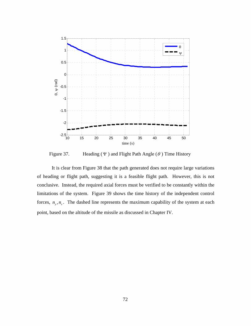
10 15 20 25 30 35 40 45 50-2.5

-2

-1.5

-1

-0.5

0

0.5

1

1.5

time (s)

θ, ψ

(rad

)

θψ

Figure 37. Heading (Ψ ) and Flight Path Angle (θ ) Time History

It is clear from Figure 38 that the path generated does not require large variations

of heading or flight path, suggesting it is a feasible flight path. However, this is not

conclusive. Instead, the required axial forces must be verified to be constantly within the

limitations of the system. Figure 39 shows the time history of the independent control

forces, . The dashed line represents the maximum capability of the system at each

point, based on the altitude of the missile as discussed in Chapter IV.

,y zn n

72

10 15 20 25 30 35 40 45 50-40

-30

-20

-10

0

10

20

30

40

time (s)

forc

e (g

)

nynz

Figure 38. Control Forces Time History

It is clear from Figure 39 that the missile is capable of navigating the generated

flight path. Note that it uses the full capabilities of the missile to conduct the

interception, which suggests that the program is appropriately accounting for the missile

capabilities. Also note that the required forces are near zero at the intercept point,

demonstrating no flair maneuver or high-g maneuver was conducted. This suggests that

the full kinematic energy of the missile is directed into the target, which was the original

intent of the program.

It can be proven that the penalty functions were indeed influencing the choice of

trajectory. If the required control effort exceeded the maximum capabilities of the

missile the trajectory, the path should be rejected as infeasible. It can be seen from

Figure 40 that this is the case, and that the final path has no penalty assigned to it.

73

0 10 20 30 40 50 60 700

1

2

3

4

5

6x 106

Iterations (#)

Pena

lty V

alue

s

PyPz

Figure 39. Penalty Function Values

The flight path is feasible, it accomplishes the intended goal, and is within the

capabilities of the interceptor missile. The final question, then, is whether the generated

flight path is in fact “optimal”, i.e. the best available path. Figure 41 shows the value of

the CF after each iteration, with emphasis on the final series of values. The figure clearly

demonstrates that the value of the CF quickly gets within the neighborhood of the

minimum, and after a short duration reaches the minimum cost function.

74

0 10 20 30 40 50 60 700

1

2

3

4

5

6x 10

6

Iterations (#)

Cost

Func

tion

Val

ue

Figure 40. Iterative Value of the Cost Function

It is also important to ensure the impact angle is maximized. It has already been

shown from the various graphs that the impact angle is indeed close to 90 degrees. It

remains to be seen, however, if it the best one that can be found. It is possible that this

flight path is returned as “optimal” not because it maximizes the impact angle, but instead

because the values of tgo and fτ dominate to the point that impact angle’s contribution is

negligible. Figure 42 shows the value of the impact angle after each iteration of the

program, with emphasis on the final values.

75

0 10 20 30 40 50 60 700

10

20

30

40

50

60

70

80

90

100

Iterations (#)

Impa

ct A

ngle

Figure 41. Iterative Value of the Cosine of the Impact Angle

The two remaining variables to be optimized have no target value, as there was

with the impact angle. It therefore must only be shown that the algorithm has indeed

tried numerous values and found the best one. Figure 43 shows the iterative value of tgo,

and clearly shows this is occurring. Likewise for Figure 44 regarding fτ .

76

0 10 20 30 40 50 60 7050

55

60

65

70

75

Iterations (#)

t go

Figure 42. Iterative Value of Intercept Time

0 10 20 30 40 50 60 7020

25

30

35

40

45

50

55

Iterations (#)

τ f

Figure 43. Iterative Value of fτ

77

78

It can therefore be said that the generated flight path is indeed the solution which

minimizes the flight path distance, minimizes the time of flight, and maximizes the

impact angle – the optimum one for this intercept.

B. APPLICABILITY This algorithm can easily be incorporated into existing control systems for

numerous applications. Yakimenko has shown that for short term spatial maneuvers, the

system is extremely robust and capable, and requires only a moderate level of

computational power [Ref 19]. The power required for this particular application is

slightly more since the final boundary conditions are not fixed but instead vary with the

time and flight path conditions. Still, a dedicated system, such as onboard a properly

modified SM-6, must be capable of not only deriving the flight path, but also storing the

data and executing it. None of these are particularly challenging requirements, as many

other missiles in the US inventory complete many of these individual tasks already.

This program cannot take into account the future actions of the target. It is thus

not applicable to a target that is capable of maneuvering or deviating from its flight path

in a considerable manner. This limits the scope and applicability of the program, but

there are currently many very capable guidance laws for these situations. The purpose

here was to propose a law that is very specific in its application but which operates far

beyond the capabilities of otherwise excellent guidance laws.

C. SUGGESTIONS FOR FUTURE RESEARCH Several avenues remain unexplored within this area of study. Some weaknesses

that may be overcome by further research are:

1. Perform a trade-off analysis of cost function weighting coefficients to

determine if the chosen ones are the most influential choices, or if they are

redundant, or if other choices may provide better results.

2. Implement a second-order prediction model of the Ballistic Missile path in the

development of the final boundary conditions to improve the accuracy of the

interception.

79

3. Perform robustness analysis using the developed 6DOF high-fidelity model

and auto-pilot model in the presence of disturbances.

4. Perform Monte Carlo simulation on launch-interception scenario to determine

the limitations on the algorithm.

80


81

APPENDIX A: MODELING PROGRAMS

A. 3DOF TARGET

1. BRParams3.m function [BR_mass,dia,length]=BRParams3(t) % Written by LT John A. Lukacs IV, Naval Postgraduate School, June 2006 % This function calculates the mass of the rocket, assuming a cruciform % rocket in two stages plus an unpowered nosecone stage. This function % also returns the reference (base) diameter of the missile. %% Notes: % The first stage last 125 seconds, the second stage lasts an % additional 110 seconds. The stages separate upon completion. %% Variable List % BR_mass =total rocket mass % BR_nose =total mass of nosecone section % BR_st1_bt =burntime for stage 1 % BR_st1_fcr =consumption rate of stage 1 fuel % BR_st1_fuel =remaining stage 1 fuel based on time and % consumption rate % BR_st1_str =total mass of stage 1 structural material % BR_st1_tfm =total mass of stage 1 fuel % BR_st2_bt =burntime for stage 2 % BR_st2_fcr =consumption rate of stage 2 fuel % BR_st2_fuel =remaining stage 2 fuel based on time and % consumption rate % BR_st2_str =total mass of stage 2 structural material % BR_st2_tfm =total mass of stage 2 fuel % dia =reference diameter, base diameter % t =time %% Structural Components BR_nose=250; BR_st2_str=2288; BR_st1_str=9000; %% Fuel Components BR_st1_tfm=50970; BR_st1_bt=125; BR_st1_fcr=BR_st1_tfm/BR_st1_bt; BR_st2_tfm=12912; BR_st2_bt=110; BR_st2_fcr=BR_st2_tfm/BR_st2_bt; if t<125 %% Stage 1 - Stage 1 Fuel is consumed; Stage 2 Fuel is not used. BR_st1_fuel=BR_st1_tfm-BR_st1_fcr*t; BR_mass=BR_nose+BR_st1_str+BR_st1_fuel+BR_st2_str+BR_st2_tfm; dia=2.2; length=2+14+16;

82

elseif t<240; %% Stage 2 - Stage 1 has separated; Stage 2 Fuel is consumed. BR_st2_fuel=BR_st2_tfm-BR_st2_fcr*(t-125); BR_mass=BR_nose+BR_st2_str+BR_st2_fuel; dia=1.3; length=2+14; else %% Stage 3 - Stage 2 has separated; unpowered nosecone remains. BR_mass=BR_nose; dia=1.3; length=2; end return

2. BRFlight3.m %% Script File % Written by LT John A. Lukacs IV, Naval Postgraduate School, June 2006 % This script integrates the position, velocity, and acceleration values % at each time step to determine the flight path of a ballistic missile % in a gravity turn. The script calls BRParams3.m, ZLDragC.m, and % STatmos.m %% Variable List % acc =total acceleration % alt =altitude % ax =x component of acceleration % ay =y component of acceleration % az =z component of acceleration % CD =drag coefficient % dia =reference diameter (base diameter) % Drag =total drag force % dt =time step interval % g =gravity force, based on WGS-84 value of gravitational % attraction and altitude % gm =initial launch angle % i =interval count % m_r =rocket mass % Mspd =rocket speed in Mach (relative to local speed of sound) % num_BR =number of iterations conducted (used for plotting) % nx =axial force % press =local atmospheric pressure % px =x component of position % py =y component of position % pz =z component of position % Re =WGS-84 value for Earth's radius % ro =local atmospheric density % spd =rocket speed in m/s % Sref =planar reference area (for drag calculations) % t =time

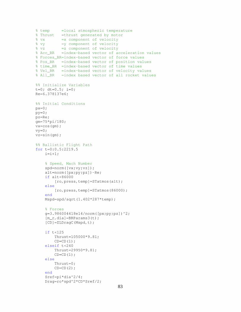
83

% temp =local atmospheric temperature % Thrust =thrust generated by motor % vx =x component of velocity % vy =y component of velocity % vz =z component of velocity % Acc_BR =index-based vector of acceleration values % Forces_BR=index-based vector of force values % Pos_BR =index-based vector of position values % time_BR =index-based vector of time values % Vel_BR =index-based vector of velocity values % All_BR =index based vector of all rocket values %% Initialize Variables t=0; dt=0.5; i=0; Re=6.378137e6; %% Initial Conditions px=0; py=0; pz=Re; gm=75*pi/180; vx=cos(gm); vy=0; vz=sin(gm); %% Ballistic Flight Path for t=0:0.5:2219.5 i=i+1; % Speed, Mach Number spd=norm([vx;vy;vz]); alt=norm([px;py;pz])-Re; if alt<86000 [ro,press,temp]=STatmos(alt); else [ro,press,temp]=STatmos(86000); end Mspd=spd/sqrt(1.402*287*temp); % Forces g=3.986004418e14/norm([px;py;pz])^2; [m_r,dia]=BRParams3(t); [CD]=ZLDragC(Mspd,t); if t<125 Thrust=105000*9.81; CD=CD(1); elseif t<240 Thrust=29950*9.81; CD=CD(1); else Thrust=0; CD=CD(2); end Sref=pi*dia^2/4; Drag=ro*spd^2*CD*Sref/2;

84

nx=(Thrust-Drag)/m_r; % Accelerations g=3.986004418e14*pz/norm([px;py;pz])^3; ax=nx*cos(gm); ay=0; az=nx*sin(gm)-g; acc=norm([ax;ay;az]); % Collect Variables time_BR(i,1)=t; Pos_BR(i,1)=px; Pos_BR(i,2)=py; Pos_BR(i,3)=pz; Pos_BR(i,4)=norm([px;py;pz]); Vel_BR(i,1)=vx; Vel_BR(i,2)=vy; Vel_BR(i,3)=vz; Vel_BR(i,4)=spd; Vel_BR(i,5)=Mspd; Acc_BR(i,1)=ax; Acc_BR(i,2)=ay; Acc_BR(i,3)=az; Acc_BR(i,4)=acc; Acc_BR(i,5)=nx; Forces_BR(i,1)=Thrust; Forces_BR(i,2)=m_r; Forces_BR(i,3)=Drag; % Time Step px=px+dt*vx; py=py+dt*vy; pz=pz+dt*vz; vx=vx+dt*ax; vy=vy+dt*ay; vz=vz+dt*az; num_BR=length(time_BR); end AllBR=[time_BR Forces_BR Pos_BR Vel_BR Acc_BR]; clear CD Drag Mspd Re Sref Thrust acc alt ax ay az dia dt clear g gm h i m_r nx press px py pz ro spd t temp vx vy vz

85

B. 3DOF INTERCEPTOR

1. SMParams3.m function [SM_mass,dia]=SMParams3(t) % Written by LT John A. Lukacs IV, Naval Postgraduate School, June 2006 % This function calculates the J Matrix and Mass of the interceptor, % assuming a cruciform rocket in two stages to intercept. This % function also returns the reference (base) diameter of the missile. %% Notes: % The first stage last 6 seconds, the second stage lasts an additional % 10 seconds. Stage 1 (booster) separates upon completion. Stage 2 % does not separate after completion % Variable List % dia =reference diameter, base diameter % l =length, varies by component % p_SM_st1_fuel=density of stage 1 rocket fuel % p_SM_st2_fuel=density of stage 2 rocket fuel % p_SMstr =density of structural material % r =radius, varies by component % ro =outer radius, varies by component % ri =inner radius, varies by component % SM_mass =total rocket mass % SM_nose =total mass of nosecone section % SM_st1_fcr =consumption rate of stage 1 fuel % SM_st1_fuel =remaining stage 1 fuel based on time and % consumption rate % SM_st1_str =total mass of stage 1 structural material % SM_st1_tfm =total mass of stage 1 fuel % SM_st2_fcr =consumption rate of stage 2 fuel % SM_st2_fuel =remaining stage 2 fuel based on time and % consumption rate % SM_st2_str =total mass of stage 2 structural material % SM_st2_tfm =total mass of stage 2 fuel % t =time % th =structural thickness % V_body =volume of body structural material % V_nose_str =volume of nosecone structural material % V_nose_str0 =volume of nosecone structural material, % intermediate value % V_nose_str1 =volume of nosecone structural material, % intermediate value % V_st1_fuel =volume of stage 1 fuel % V_st1_str =volume of stage 1 structural material % V_st2_fuel =volume of stage 2 fuel % V_st2_str =volume of stage 2 structural material %% Structural Components p_SMstr=4225; th=.0208; % Mass of Nosecone l=.8255;

86

r=0.34/2; V_nose_str0=pi*(l*((r^2+l^2)/(2*r))^2-l^3/3-(((r^2+l^2)/... (2*r))-r)*((r^2+l^2)/(2*r))^2*asin(l/((r^2+l^2)/(2*r)))); l=.8255-th; r=0.34/2-th; V_nose_str1=pi*(l*((r^2+l^2)/(2*r))^2-l^3/3-(((r^2+l^2)/... (2*r))-r)*((r^2+l^2)/(2*r))^2*asin(l/((r^2+l^2)/(2*r)))); V_nose_str=V_nose_str0-V_nose_str1+pi*r^2*th; SM_nose=1.3*V_nose_str*p_SMstr; % Mass of Body/Warhead Section l=.849; ro=0.34/2; ri=0.34/2-th; V_body=l*pi*(ro^2-ri^2); SM_body=V_body*p_SMstr+115; % Mass of Stage 1 (Mk72 Booster) l=1.72; ro=0.53/2; ri=0.53/2-th; V_st1_str=l*pi*(ro^2-ri^2)+2*pi*ro^2*th; SM_st1_str=V_st1_str*p_SMstr; % Mass of Stage 2 (Mk104 Engine) l=2.88-2*th; ro=0.34/2; ri=0.34/2-th; V_st2_str=l*pi*(ro^2-ri^2)+2*pi*ro^2*th; SM_st2_str=V_st2_str*p_SMstr; %% Fuel Components % Stage 1 Solid Fuel is HTPB/AP/Al l=1.72; ri=0.53/2-th; V_st1_fuel=0.80*l*pi*ri^2; p_SM_st1_fuel=1860; SM_st1_tfm=468; SM_st1_fcr=468/6; % Stage 2 Solid Fuel is TP-H1205/6 l=2.88; ri=0.34/2-th; V_st2_fuel=0.60*l*pi*ri^2; SM_st2_tfm=360; p_SM_st2_fuel=SM_st2_tfm/V_st2_fuel; SM_st2_fcr=360/15; if t<6 %% Stage 1 - Stage 1 Fuel is consumed; Stage 2 Fuel is not used. SM_st1_fuel=SM_st1_tfm - SM_st1_fcr * t; SM_mass=SM_nose+SM_body+SM_st2_str+SM_st2_tfm+SM_st1_str+... SM_st1_fuel; dia=0.53; elseif t<21 %% Stage 2 - Stage 1 has separated; Stage 2 Fuel is consumed.

87

SM_st2_fuel=SM_st2_tfm - SM_st2_fcr * (t-6); SM_mass=SM_nose+SM_body+SM_st2_str+SM_st2_fuel; dia=0.34; else %% Stage 3 - The unpowered nosecone and Stage 2 remains. SM_mass=SM_nose+SM_body+SM_st2_str; dia=0.34; end return

2. SMFlight3.m %% Script File % Written by LT John A. Lukacs IV, Naval Postgraduate School, June 2006 % This script develops and tracks the flight path of the interceptor % missile. For the first ten seconds it integrates a series of % acceleration commands to simulate a vertical launch and tip over. % Upon activation of the guidance law, it sends the known values to the % guidance law and receives back the future time history of the optimal % flight path. This script then implements that optimal path. It % updates the final conditions and recalculates the optimal flight path % at an (modifiable) interval of 10 seconds. The script calls % SMParams3.m, ZLDragC.m, and STatmos.m %% Variable List % Acc_SM =index-based vector of acceleration values % AllSM =index based vector of all interceptor values % alt =altitude % CD =drag coefficient % count =counting variable to determine guidance law update % interval % dia =reference diameter (base diameter) % dist =cumulative distance traveled % Drag =total drag force % Forces_SM=index-based vector of force values % g =gravity force, based on WGS-84 value of % gravitational attraction and altitude % i =interval count % m_i =interceptor mass % Model_SM =index-based vector of internal values % MV =interceptor speed in Mach (relative to local speed of % sound) % N1 =variable used to compare optimal vector length % N2 =variable used to compare optimal vector length % num_SM =number of iterations conducted (used for plotting) % nx =axial acceleration command, body frame x % nx_Op =index based vector of the optimal flight path values % ny =axial acceleration command, body frame y % ny_Op =index based vector of the optimal flight path values % nz =axial acceleration command, body frame z % nz_Op =index based vector of the optimal flight path values

88

% path =returned time history of the optimal path % Pos_SM =index-based vector of position values % press =local atmospheric pressure % psi =heading angle % psi_old =heading angle (used in the time step) % psi_Op =index based vector of the optimal flight path values % psidot =rate of change of heading angle % psidot_Op=index based vector of the optimal flight path values % px =x component of position % px_old =x component of position (used in the time step) % px_Op =index based vector of the optimal flight path values % py =y component of position % py_old =y component of position (used in the time step) % py_Op =index based vector of the optimal flight path values % pz =z component of position % pz_old =z component of position (used in the time step) % pz_Op =index based vector of the optimal flight path values % q =counting variable (used in another program) % Re =WGS-84 Earth's radius % ro =local atmospheric density % spot =counting variable (used for plotting) % spot2 =counting variable (used for plotting) % Sref =planar reference area (for drag calculations) % state =the state of the interceptor % t =time % target =the state of the rocket % temp =local atmospheric temperature % tgo =time to go to intercept % th =flight path angle % th_old =flight path angle (used in the time step) % th_Op =index based vector of the optimal flight path values % thdot =rate of change of flight path angle % thdot_Op =index based vector of the optimal flight path values % Thrust =thrust generated by motor % time_Op =index based vector of the optimal flight path values % time_SM =index-based vector of time values % update =number of updates to the guidance law conducted % V =velocity of the interceptor % V_old =velocity of the interceptor (used in the time step) % V_Op =index based vector of the optimal flight path values % Vdot =rate of change of the velocity % Vdot_Op =index based vector of the optimal flight path values % Vel_SM =index-based vector of velocity values % w =counting variable (used in another program) BRFlight3 global tgo q states xf xpf spot spot2 j path N1 update trys global spot spot2 w Pos_BR Pos_SM % Initialize Variables t=0; dt=0.5; i=0; ii=0; w=120; q=0; qq=0; rr=0; count=30; update=0 ;spot=13; spot2=81; Re=6.378137e6;

89

tgo=85; V=1; psi=-130*pi/180; th=90*pi/180; V_old=V; psi_old=psi; th_old=th; px=100000; py=100000; pz=Re; px_old=px; py_old=py; pz_old=pz; dist=0; %% Flight Path for i=1:1:1000 t=t+dt; % True APN Guidance if t<10 % Speed, Mach Number alt=norm([px;py;pz])-Re; if alt<86000 [ro, press, temp]=STatmos(alt); else [ro, press, temp]=STatmos(86000); end MV=V/sqrt(1.402*287*temp); % Forces g=3.986004418e14/norm([px;py;pz])^2; [m_i,dia]=SMParams3(t); [CD]=ZLDragC(MV,t); if t<6 Thrust=206500; CD=CD(1); elseif t<20 Thrust=95300; CD=CD(1); else Thrust=0; CD=CD(2); end Sref=pi*dia^2/4; Drag=ro*V^2*CD*Sref/2; nx=(Thrust-Drag)/m_i/g; % Guidance if t<=6 % Boost Phase Vertical Launch psidot=0; thdot=0; ny=V/g*cos(th)*psidot ; nz=V/g*thdot+cos(th);

90

else % Boost Phase Pitch over psidot=0; thdot=-0.075; ny=V/g*cos(th)*psidot; nz=V/g*thdot+cos(th); end % Kinematics Vdot=g*(nx-sin(th)); psidot=ny*g/V/cos(th); thdot=g*(nz-cos(th))/V; % Collect Variables time_SM(i,1)=t; Forces_SM(i,1)=nx; Forces_SM(i,2)=ny; Forces_SM(i,3)=nz; Model_SM(i,1)=V; Model_SM(i,2)=Vdot; Model_SM(i,3)=th; Model_SM(i,4)=thdot; Model_SM(i,5)=psi; Model_SM(i,6)=psidot; Pos_SM(i,1)=px; Pos_SM(i,2)=py; Pos_SM(i,3)=pz; Pos_SM(i,4)=dist; Vel_SM(i,1)=V*cos(th)*cos(psi); Vel_SM(i,2)=V*cos(th)*sin(psi); Vel_SM(i,3)=V*sin(th); Acc_SM(i,1)=Vdot*cos(th)*cos(psi)-V*cos(th)*sin(psi)*psidot... -V*sin(th)*cos(psi)*thdot; Acc_SM(i,2)=Vdot*cos(th)*sin(psi)+V*cos(th)*cos(psi)*psidot... +V*sin(th)*sin(psi)*thdot; Acc_SM(i,3)=Vdot*sin(th)+V*cos(th)*thdot; % Time Step V=V_old+Vdot*dt; psi=psi_old+psidot*dt; th=th_old+thdot*dt; px=px_old+V*cos(th)*cos(psi)*dt; py=py_old+V*cos(th)*sin(psi)*dt; pz=pz_old+V*sin(th)*dt; dist=(dist+abs(norm([px-px_old;py-py_old;pz-pz_old]))); V_old=V; psi_old=psi; th_old=th; px_old=px; py_old=py; pz_old=pz;

91

else % Optimal Guidance if count==30 display('Starting SMGuidance Update') update=update+1; state=[px;py;pz;V;th;psi;Vdot;thdot;psidot]; target=[Pos_BR(i+w,1);Pos_BR(i+w,2);Pos_BR(i+w,3); Vel_BR(i+w,1);Vel_BR(i+w,2);Vel_BR(i+w,3)]; [path]=SMGuidance(t,state,target,i); if update==1; N1=length(path(:,1)); N2=N1; else N2=length(path(:,1)); end % Identify Variables time_Op(:,update)=[path(:,1);zeros(N1-N2,1)]; px_Op(:,update)=[path(:,2);zeros(N1-N2,1)]; py_Op(:,update)=[path(:,3);zeros(N1-N2,1)]; pz_Op(:,update)=[path(:,4);zeros(N1-N2,1)]; V_Op(:,update)=[path(:,5);zeros(N1-N2,1)]; th_Op(:,update)=[path(:,6);zeros(N1-N2,1)]; psi_Op(:,update)=[path(:,7);zeros(N1-N2,1)]; Vdot_Op(:,update)=[path(:,8);zeros(N1-N2,1)]; thdot_Op(:,update)=[path(:,9);zeros(N1-N2,1)]; psidot_Op(:,update)=[path(:,10);zeros(N1-N2,1)]; nx_Op(:,update)=[path(:,11);zeros(N1-N2,1)]; ny_Op(:,update)=[path(:,12);zeros(N1-N2,1)]; nz_Op(:,update)=[path(:,13);zeros(N1-N2,1)]; count=1; end t=time_Op(count,update); nx=nx_Op(count,update); ny=ny_Op(count,update); nz=nz_Op(count,update); V=V_Op(count,update); Vdot=Vdot_Op(count,update); th=th_Op(count,update); thdot=thdot_Op(count,update); psi=psi_Op(count,update); psidot=psidot_Op(count,update); px=px_Op(count,update); py=py_Op(count,update); pz=pz_Op(count,update); % Collect Variables time_SM(i,1)=t; Forces_SM(i,1)=nx; Forces_SM(i,2)=ny; Forces_SM(i,3)=nz; Model_SM(i,1)=V; Model_SM(i,2)=Vdot; Model_SM(i,3)=th; Model_SM(i,4)=thdot; Model_SM(i,5)=psi; Model_SM(i,6)=psidot; Pos_SM(i,1)=px;

92

Pos_SM(i,2)=py; Pos_SM(i,3)=pz; Pos_SM(i,4)=dist; Vel_SM(i,1)=V*cos(th)*cos(psi); Vel_SM(i,2)=V*cos(th)*sin(psi); Vel_SM(i,3)=V*sin(th); Acc_SM(i,1)=Vdot*cos(th)*cos(psi)-V*cos(th)*sin(psi)*psidot... -V*sin(th)*cos(psi)*thdot; Acc_SM(i,2)=Vdot*cos(th)*sin(psi)+V*cos(th)*cos(psi)*psidot... +V*sin(th)*sin(psi)*thdot; Acc_SM(i,3)=Vdot*sin(th)+V*cos(th)*thdot; Update(i,1)=update; % Time Step count=count+1; dist=(dist+abs(norm([px-px_old;py-py_old;pz-pz_old]))); V_old=V; psi_old=psi; th_old=th; px_old=px; py_old=py; pz_old=pz; end num_SM=length(time_SM); end AllSM= [time_SM Forces_SM Model_SM Pos_SM Vel_SM Acc_SM update];

C. 6DOF MODEL

1. BRDetails6.m %% Script File % Written by LT John A. Lukacs IV, Naval Postgraduate School, June 2006 % This script defines mass and fuel parameters of the Ballistic Rocket, % as extracted from several open source materials relating to the % North Korean Taepo-Dong II missile project. % This script calculates the volume of structural material and % therefore the weight of the structural components, assuming % structural steel as the primary structural material. The process to % determine the average thickness of the structure was an iterative % process based on the known information of launch weight, some fuel % data, payload, and burn times. %% Variables List % BR_fuel_p =density of rocket fuel % BR_str_p =density of structural material % BR_nose =total mass of nosecone section % BR_st1_bt =burn time of stage 1 fuel % BR_st1_fcr =consumption rate of stage 1 fuel % BR_st1_str =total mass of stage 1 structural material % BR_st1_tfm =total mass of stage 1 fuel

93

% BR_st2_bt =burn time of stage 2 fuel % BR_st2_fcr =consumption rate of stage 2 fuel % BR_st2_str =total mass of stage 2 structural material % BR_st2_tfm =total mass of stage 2 fuel % l =length, varies by component % r =radius, varies by component % ri =outer radius, varies by component % ro =inner radius, varies by component % tctc =total vs. chamber thrust comparison, used to % extrapolate fuel consumption rate for stage 1 % from stage 2 % th =thickness of structural material % V_nose_str =volume of nosecone structural material % V_nose_str0=volume of nosecone structural material, % intermediate value % V_nose_str1=volume of nosecone structural material, % intermediate value % V_st1_str =volume of stage 1 structural material % V_st2_str =volume of stage 2 structural material global BR_str_p BR_fuel_p BR_nose BR_st2_str BR_st1_str global BR_st2_tfm BR_st1_tfm BR_st1_fcr BR_st2_fcr %% Structural Components BR_str_p=7682; th=.012; %% Mass of Nosecone l=2; r=1.3/2; V_nose_str0=pi*(l*((r^2+l^2)/(2*r))^2+l^3/3-(((r^2+l^2)/(2*r))-r)*... ((r^2+l^2)/(2*r))^2*asin(l/((r^2+l^2)/(2*r)))); l=2-th; r=1.3/2-th; V_nose_str1=pi*(l*((r^2+l^2)/(2*r))^2+l^3/3-(((r^2+l^2)/(2*r))-r)*... ((r^2+l^2)/(2*r))^2*asin(l/((r^2+l^2)/(2*r)))); V_nose_str=V_nose_str0-V_nose_str1; BR_nose=250+V_nose_str*BR_str_p; %% Mass of Stage 2 l=14; r0=1.3/2; ri=1.3/2-th; V_st2_str=l*pi*(r0^2-ri^2); BR_st2_str=V_st2_str*BR_str_p; %% Mass of Stage 1 l=16; r0=2.2/2; ri=2.2/2-th; V_st1_str=l*pi*(r0^2-ri^2); BR_st1_str=V_st1_str*BR_str_p; %% Fuel Components BR_fuel_p=801.164+1544.9/4.05;

94

% Fuel mass, rate, burntime BR_st2_tfm=12912; BR_st2_bt=110; BR_st2_fcr=BR_st2_tfm/BR_st2_bt; tctc=103000/30432; BR_st1_fcr=BR_st2_fcr*tctc; BR_st1_bt=125;

BR_st1_tfm=BR_st1_fcr*BR_st1_bt;

2. BRParams6.m function [J,BR_mass,dia,length]=BRParams6(t) % Written by LT John A. Lukacs IV, Naval Postgraduate School, June 2006 % This function calculates the J Matrix and Mass of the rocket, % assuming a cruciform rocket in two stages plus an unpowered nosecone % stage. This function also returns the reference (base) diameter of % the missile. %% Notes: % All CGs are measured from the tip of the nosecone. % The rocket is divided into five components: the nosecone and payload, % stage one structure, stage one fuel, stage 2 structure, stage 2 fuel. % Liquid fuel is assumed to remain at the rear of the fuel tanks. Both % stages utilize the same fuel. Fuel is consumed at a constant rate. % The first stage last 130 seconds, the second stage lasts an % additional 110 seconds. The stage separates upon completion. % No Parallel axis theorem is required for Jx due to symmetry. Parallel % axis theorem is required from CG for Jy and Jz. % Variable List % BR_fuel_L =Length of remaining fuel in the stage % BR_fuel_p =density of rocket fuel % BR_mass =total rocket mass % BR_nose =total mass of nosecone section % BR_str_p =density of structural material % BR_st1_fcr =consumption rate of stage 1 fuel % BR_st1_fuel =remaining stage 1 fuel based on time and % consumption rate % BR_st1_str =total mass of stage 1 structural material % BR_st1_tfm =total mass of stage 1 fuel % BR_st2_fcr =consumption rate of stage 2 fuel % BR_st2_fuel =remaining stage 2 fuel based on time and % consumption rate % BR_st2_str =total mass of stage 2 structural material % BR_st2_tfm =total mass of stage 2 fuel % CG =total rocket center of gravity % CG_nose =nosecone center of gravity % CG_st1 =stage 1 center of gravity % CG_st2 =stage 2 center of gravity % dia =reference diameter, base diameter % J =Matrix of moment of inertia % Jx =total rocket moment of inertia, x-axis

95

% Jx_nose =nosecone moment of inertia, x-axis % Jx_st1_fuel =stage 1 fuel moment of inertia, x-axis % Jx_st1_str =stage 1 structure moment of inertia, x-axis % Jx_st2_fuel =stage 2 fuel moment of inertia, x-axis % Jx_st2_str =stage 2 structure moment of inertia, x-axis % Jy =total rocket moment of inertia, y-axis % Jy_nose =nosecone moment of inertia, y-axis % Jy_st1_fuel =stage 1 fuel moment of inertia, y-axis % Jy_st1_str =stage 1 structure moment of inertia, y-axis % Jy_st2_fuel =stage 2 fuel moment of inertia, y-axis % Jy_st2_str =stage 2 structure moment of inertia, y-axis % Jz =total rocket moment of inertia, z-axis % t =time global BR_str_p BR_fuel_p BR_nose BR_st2_str BR_st1_str global BR_st2_tfm BR_st1_tfm BR_st1_fcr BR_st2_fcr if t<130 % Stage 1 - Stage 1 Fuel is consumed; Stage 2 Fuel is not used. BR_st1_fuel=BR_st1_tfm-BR_st1_fcr*t; BR_fuel_L=BR_st1_fuel/(BR_fuel_p*pi*1.0^2); CG_nose=BR_nose*10/8; CG_st1=BR_st1_str*24+BR_st1_fuel*(32-BR_fuel_L); CG_st2=BR_st2_str*9+BR_st2_tfm*9; BR_mass=BR_nose+BR_st1_str+BR_st1_fuel+BR_st2_str+BR_st2_tfm; CG=(CG_nose+CG_st1+CG_st2)/BR_mass; FF=(BR_st1_fuel+BR_st2_tfm)/BR_mass; Jx_nose=BR_nose*3*(0.65^2)/10; Jx_st1_str=BR_st1_str*(1.1^2+1.025^2)/2; Jx_st1_fuel=BR_st1_fuel*(1.025^2)/2; Jx_st2_str=BR_st2_str*(0.65^2+0.575^2)/2; Jx_st2_fuel=BR_st2_tfm*(0.575^2)/2; Jx=Jx_nose+Jx_st1_str+Jx_st1_fuel+Jx_st2_str+Jx_st2_fuel; Jy_nose=BR_nose*3*(.25*1.3^2+2^2)+BR_nose*(CG-10/8)^2; Jy_st1_str=BR_st1_str*(16^2/12+(1.1^2+1.025^2)/4)+ ... BR_st1_str*(CG-24)^2; Jy_st1_fuel=BR_st1_fuel*(1.025^2/4 + BR_fuel_L^2/12) + ... BR_st1_fuel*(CG-(32-BR_fuel_L/12))^2; Jy_st2_str=BR_st2_str*(14^2/12+(0.65^2+0.575^2)/4)+ ... BR_st2_str*(CG-9)^2; Jy_st2_fuel=BR_st2_tfm*(0.575^2/4+7^2/12) + ... BR_st2_tfm*(CG-9)^2; Jy=Jy_nose+Jy_st1_str+Jy_st1_fuel+Jy_st2_str+Jy_st2_fuel; Jz=Jy; dia=2.2; length=2+14+16; elseif t<240; % Stage 2 - Stage 1 has separated; Stage 2 Fuel is consumed. BR_st2_fuel=BR_st2_tfm-BR_st2_fcr*(t-130); BR_fuel_L=BR_st2_fuel/(BR_fuel_p*pi*0.575^2);

96

CG_nose=BR_nose*10/8; CG_st2=BR_st2_str*9+BR_st2_fuel*(14-BR_fuel_L); BR_mass=BR_nose+BR_st2_str+BR_st2_fuel; CG=(CG_nose+CG_st2)/BR_mass; Jx_nose=BR_nose*3*(0.65^2)/10; Jx_st2_str=BR_st2_str*(0.65^2+0.575^2)/2; Jx_st2_fuel=BR_st2_fuel*(0.575^2)/2; Jx=Jx_nose+Jx_st2_str+Jx_st2_fuel; Jy_nose=BR_nose*3*(1.3^2/4+2^2)+BR_nose*(CG-10/8)^2; Jy_st2_str=BR_st2_str*(14^2/12+(0.65^2+0.575^2)/4)+ ... BR_st2_str*(CG-9)^2; Jy_st2_fuel=BR_st2_fuel*(0.575^2/4+BR_fuel_L^2/12)+ ... BR_st2_fuel*(CG-(16-BR_fuel_L/2))^2; Jy=Jy_nose+Jy_st2_str+Jy_st2_fuel; Jz=Jy; dia=1.3; length=2+14; else % Stage 3 - Stage 2 has separated; only the unpowered nosecone remains. BR_fuel_L=0; CG_nose=BR_nose*10/8; BR_mass=BR_nose; CG=(CG_nose)/BR_mass; Jx=BR_nose*3*(0.65^2)/10; Jy=BR_nose*3*(1.3^2/4+2^2)+BR_nose*(CG-10/8)^2; Jz=Jy; dia=1.3; length=2; end %% Combining the results into output variables. J=[Jx 0 0; 0 Jy 0; 0 0 Jz];

return

97

3. BRFlight6.m function [udot]=BRFlight6(u) % Written by LT John A. Lukacs IV, Naval Postgraduate School, June 2006 % This script integrates the position, velocity, and acceleration % values at each time step to determine the flight path of a ballistic % missile in a gravity turn. The script calls BRParams6.m, ZLDragC.m, % and STatmos.m % Variable List: % [ACoeff] =Vector of 13 coefficients returned from Aerocoeff.m % Aa =angle of attack % As =sideslip angle % Cd =aerodynamic coefficient % Cl =aerodynamic coefficient % Cm =aerodynamic coefficient % CN =aerodynamic coefficient % Cn =aerodynamic coefficient % CY =aerodynamic coefficient % delta_h =iterative value for determination of altitude % dia =reference diameter, base diameter % dP =Pitch control surface deflection % dPdot =Pitch control surface deflection derivative % Drag =Total drag force % dY =Yaw control surface deflection % dYdot =Yaw control surface deflection derivative % egm =intermediate value for gravity calculations % Force =Total force on the center of mass % g =Gravity % h =Altitude above the Earth surface % J =Mass Moment of Inertia Matrix % latgc =Geocentric Latitude % latgd =Geodetic Latitude % lm_g =Celestial Longitude % Mach =Ballistic Rocket speed in Mach % Mspd =Local Speed of Sound % N =iterative value for determination of altitude % Nh =iterative value for determination of altitude % P =Roll Rate % p =Ballistic Rocket Position vector, [px;py;pz] % pdot =Ballistic Rocket Position derivative vector % phi =Euler Roll wrt ECEF % press =atmospheric pressure % psy =Euler Yaw wrt ECEF % px =X Position % py =Y Position % pz =Z Position % Q =Pitch Rate % q =quaternion vector % q0 =Quaternion's 0th component % q1 =Quaternion's 1st component % q2 =Quaternion's 2nd component % q3 =Quaternion's 3rd component % qdot =Quaternion derivative % qnorm =Normalization of Quaternion % Qro =Atmospheric density

98

% R =Yaw Rate % R_b2e =Rotation Matrix % R_i2b =Rotation Matrix % R_i2e =Rotation Matrix % R_n2b =Rotation Matrix % Rm =Ballistic Rocket current mass % ro =local atmospheric density % rp =iterative value for gravity % speed =velocity of the rocket in m/s % t =time % theta =Euler Pitch wrt ECEF % temp =local atmospheric temperature % Thrust =thrust vector % Torque =torque vecto r% u =input vector % udot =output vector, to be integrated % vb =velocity vector % vdot =velocity vector derivative % vx =X Velocity % vy =Y Velocity % vz =Z Velocity % wb =angular velocity % Wbwi =cross product matrix % wdot =angular velocity derivative % Wewi =cross product matrix % Wq =cross product matrix global lLong Re WzE Eps2 Gravity R_e2n runcount dq dr % Variable Definitions and Quaternion Normalization px=u(1); py=u(2); pz=u(3); vx=u(4); vy=u(5); vz=u(6); P =u(7); Q =u(8); R =u(9); qnorm=norm(u(10:13),2); q0=u(10)/qnorm; q1=u(11)/qnorm; q2=u(12)/qnorm; q3=u(13)/qnorm; t =u(14); dq=u(15); dr=u(16); % Vector Definitions p =[px;py;pz]; vb=[vx;vy;vz]; wb=[P;Q;R]; q =[q0;q1;q2;q3]; % Geocentric Latitude and Celestial Longitude from [p] latgc=atan(pz/sqrt(px^2+py^2));

99

lm_g=(atan2(py,px)+lLong-WzE*t); if lm_g > pi lm_g=lm_g-pi; elseif lm_g < -pi lm_g=lm_g+pi; end % Geodetic Latitude and Altitude about the Earth's Geoid from [p] h=0; N=Re; Nh=N+h; delta_h=Re; while abs(delta_h) > .1 latgd=atan(pz/sqrt(px^2+py^2)/(1-N*Eps2/Nh)); N=Re/sqrt(1-Eps2*sin(latgd)^2); Nh=sqrt(px^2+py^2)/cos(latgd); delta_h=Nh-N-h; h=h+delta_h; end % Gravity, Atmosphere from EGM1996 rp=norm(p,2); egm=diag([1;1;3]); g=-Gravity*3.986004418e14/rp^2*(eye(3)+1.5*1.0826267e-3*(Re/rp)^2*... (egm-5*(pz/rp)^2*eye(3)))*p/rp; [ro,press,temp]=STatmos(h); % Speed, Mach Number, Angles speed=norm(vb,2); Mspd=sqrt(1.402*287*temp); Mach=speed/Mspd; Aa=atan2(vz,vx); As=atan2(vy,speed); if As<1e- 3 As=0; end % Moment Matrix, Aerodynamic Coefficients [J,Rm,dia,length]=BRParams(t); CD=ZLDragC(Mach,t); Sref=pi*dia^2/4; Drag=ro*speed*vb*CD*Sref/2; Qro=0.5*ro*speed^2; [CN_Aa Cm_Aa CY_As Cn_As Cl_dp CY_dp Cn_dp... Cl_dr CY_dr Cn_dr Cl_As CN_dq Cm_dq]=AeroCoeff(Aa,h,dq,t); CY=CY_As*As+CY_dr*dr; CN=CN_Aa*Aa+CN_dq*dq; Cl=Cl_As*As+Cl_dr*dr+dia/2*speed*[-0.5*P]; Cm=Cm_Aa*Aa+Cm_dq*dq+dia/2*speed*[-0.5*Q]; Cn=Cn_As*As+Cn_dr*dr+dia/2*speed*[-0.5*R]; % Force, Torque if t < 130 Thrust=[103500*9.81;0;0]; elseif t < 240

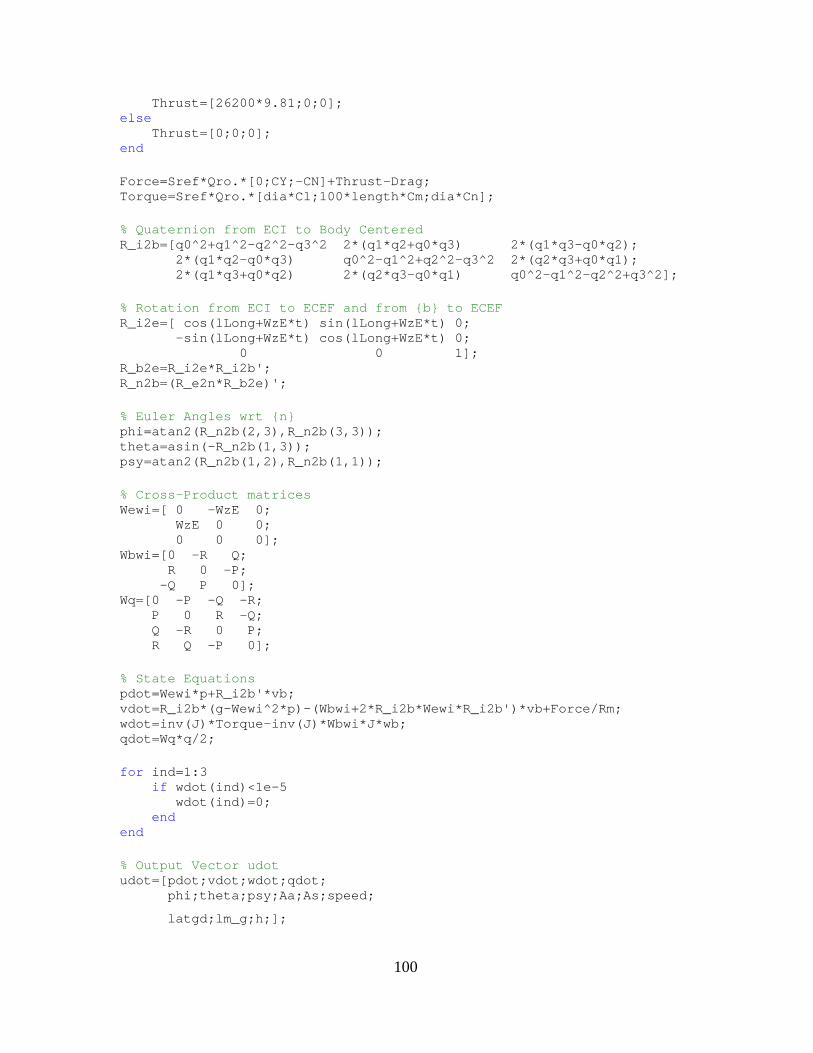
100

Thrust=[26200*9.81;0;0]; else Thrust=[0;0;0]; end Force=Sref*Qro.*[0;CY;-CN]+Thrust-Drag; Torque=Sref*Qro.*[dia*Cl;100*length*Cm;dia*Cn]; % Quaternion from ECI to Body Centered R_i2b=[q0^2+q1^2-q2^2-q3^2 2*(q1*q2+q0*q3) 2*(q1*q3-q0*q2); 2*(q1*q2-q0*q3) q0^2-q1^2+q2^2-q3^2 2*(q2*q3+q0*q1); 2*(q1*q3+q0*q2) 2*(q2*q3-q0*q1) q0^2-q1^2-q2^2+q3^2]; % Rotation from ECI to ECEF and from b to ECEF R_i2e=[ cos(lLong+WzE*t) sin(lLong+WzE*t) 0; -sin(lLong+WzE*t) cos(lLong+WzE*t) 0; 0 0 1]; R_b2e=R_i2e*R_i2b'; R_n2b=(R_e2n*R_b2e)'; % Euler Angles wrt n phi=atan2(R_n2b(2,3),R_n2b(3,3)); theta=asin(-R_n2b(1,3)); psy=atan2(R_n2b(1,2),R_n2b(1,1)); % Cross-Product matrices Wewi=[ 0 -WzE 0; WzE 0 0; 0 0 0]; Wbwi=[0 -R Q; R 0 -P; -Q P 0]; Wq=[0 -P -Q -R; P 0 R -Q; Q -R 0 P; R Q -P 0]; % State Equations pdot=Wewi*p+R_i2b'*vb; vdot=R_i2b*(g-Wewi^2*p)-(Wbwi+2*R_i2b*Wewi*R_i2b')*vb+Force/Rm; wdot=inv(J)*Torque-inv(J)*Wbwi*J*wb; qdot=Wq*q/2; for ind=1:3 if wdot(ind)<1e-5 wdot(ind)=0; end end % Output Vector udot udot=[pdot;vdot;wdot;qdot; phi;theta;psy;Aa;As;speed;

latgd;lm_g;h;];

101

3. SMDetails6.m %% Script File % Written by LT John A. Lukacs IV, Naval Postgraduate School, June 2006 % This script defines mass and fuel parameters of the SM-6 interceptor % missile, as extracted from several open source materials relating to % the Raytheon SM-6 ERAAW interceptor missile project. % This script calculates the volume of structural material and % therefore weight of the structural components, assuming structural % steel as the primary structural material. The process to determine % the average thickness of the structure was an iterative process based % on the known information of launch weight, some fuel data, payload, % and burn times. %% Variables List % l =length, varies by component % p_SM_st1_fuel=density of stage 1 rocket fuel % p_SM_st2_fuel=density of stage 2 rocket fuel % p_SMstr =density of structural material % r =radius, varies by component % r0 =outer radius, varies by component % ri =inner radius, varies by component % SM_body =total mass of body section % SM_nose =total mass of nosecone section % SM_st1_fr =fuel consumption rate of stage1 % SM_st1_str =total mass of stage 1 structural material % SM_st1_tfm =total fuel mass of stage 1 % SM_st2_fr =fuel consumption rate of stage2 % SM_st2_str =total mass of stage 2 structural material % SM_st2_tfm =total fuel mass of stage 2 % th =thickness of structural material % V_body =volume of body structural material % V_nose_str =volume of nosecone structural material % V_nose_str0 =volume of nosecone structural material, % intermediate value % V_nose_str1 =volume of nosecone structural material, % intermediate value % V_st1_fuel =volume of stage 1 fuel % V_st1_str =volume of stage 1 structural material % V_st2_fuel =volume of stage 2 fuel % V_st2_str =volume of stage 2 structural material global p_SMstr p_SM_st2_fuel p_SM_st1_fuel SM_nose SM_st2_str global SM_st1_str SM_body SM_st2_tfm SM_st1_tfm SM_st1_fr SM_st2_fr %% Structural Components p_SMstr=7682; th=.007; % Mass of Nosecone l=.8255; r=0.34/2;

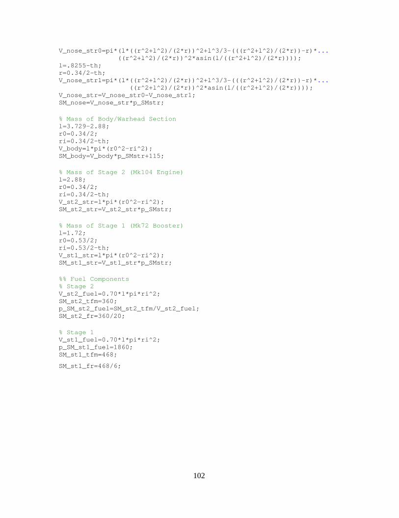
102

V_nose_str0=pi*(l*((r^2+l^2)/(2*r))^2+l^3/3-(((r^2+l^2)/(2*r))-r)*... ((r^2+l^2)/(2*r))^2*asin(l/((r^2+l^2)/(2*r)))); l=.8255-th; r=0.34/2-th; V_nose_str1=pi*(l*((r^2+l^2)/(2*r))^2+l^3/3-(((r^2+l^2)/(2*r))-r) *... ((r^2+l^2)/(2*r))^2*asin(l/((r^2+l^2)/(2*r)))); V_nose_str=V_nose_str0-V_nose_str1; SM_nose=V_nose_str*p_SMstr; % Mass of Body/Warhead Section l=3.729-2.88; r0=0.34/2; ri=0.34/2-th; V_body=l*pi*(r0^2-ri^2); SM_body=V_body*p_SMstr+115; % Mass of Stage 2 (Mk104 Engine) l=2.88; r0=0.34/2; ri=0.34/2-th; V_st2_str=l*pi*(r0^2-ri^2); SM_st2_str=V_st2_str*p_SMstr; % Mass of Stage 1 (Mk72 Booster) l=1.72; r0=0.53/2; ri=0.53/2-th; V_st1_str=l*pi*(r0^2-ri^2); SM_st1_str=V_st1_str*p_SMstr; %% Fuel Components % Stage 2 V_st2_fuel=0.70*l*pi*ri^2; SM_st2_tfm=360; p_SM_st2_fuel=SM_st2_tfm/V_st2_fuel; SM_st2_fr=360/20; % Stage 1 V_st1_fuel=0.70*l*pi*ri^2; p_SM_st1_fuel=1860; SM_st1_tfm=468;

SM_st1_fr=468/6;

103

5. SMParams6.m function [J,SM_mass,C]=SMParams6(t) % Written by LT John A. Lukacs IV, Naval Postgraduate School, June 2006 % This function calculates the J Matrix and Mass of the interceptor, % assuming a cruciform rocket in two stages to intercept. This % function also returns the reference (base) diameter of the missile. %% Notes: % All CGs are measured from the tip of the nosecone. % The rocket is divided into five components: the nosecone and payload, % stage one structure, stage one fuel, stage 2 structure, stage 2 fuel. % Solid fuel is assumed to burn from the centerline radially outward. % A constant burn profile is assumed, such as a star grain produces. % See description in SMDetail.m for specific derivation of reasons. % The first stage last 6 seconds, the second stage lasts an additional % 15 seconds. Stage 1 (booster) separates upon completion. Stage 2 % does not separate after completion. % Variable List: % SM_mass =total rocket mass % SM_nose =total mass of nosecone section % SM_st1_fcr =consumption rate of stage 1 fuel % SM_st1_fuel =remaining stage 1 fuel based on time and % consumption rate % SM_st1_str =total mass of stage 1 structural material % SM_st1_tfm =total mass of stage 1 fuel % SM_st2_fcr =consumption rate of stage 2 fuel % SM_st2_fuel =remaining stage 2 fuel based on time and % consumption rate % SM_st2_str =total mass of stage 2 structural material % SM_st2_tfm =total mass of stage 2 fuel % CG =total rocket center of gravity % CG_nose =nosecone center of gravity % CG_st1 =stage 1 center of gravity % CG_st2 =stage 2 center of gravity % dia =reference diameter, base diameter % J =Matrix of moment of inertia % Jx =total rocket moment of inertia, x-axis % Jx_nose =nosecone moment of inertia, x-axis % Jx_st1_fuel =stage 1 fuel moment of inertia, x-axis % Jx_st1_str =stage 1 structure moment of inertia, x-axis % Jx_st2_fuel =stage 2 fuel moment of inertia, x-axis % Jx_st2_str =stage 2 structure moment of inertia, x-axis % Jy =total rocket moment of inertia, y-axis % Jy_nose =nosecone moment of inertia, y-axis % Jy_st1_fuel =stage 1 fuel moment of inertia, y-axis % Jy_st1_str =stage 1 structure moment of inertia, y-axis % Jy_st2_fuel =stage 2 fuel moment of inertia, y-axis % Jy_st2_str =stage 2 structure moment of inertia, y-axis % Jz =total rocket moment of inertia, z-axi s% L_SMfuel =Length of remaining fuel in the stage % p_SMfuel =density of rocket fuel % p_SMstr =density of structural material

104

% t =time global p_SMstr p_SM_st1_fuel p_SM_st2_fuel SM_nose SM_st2_str global SM_st1_str SM_body SM_st2_fuel_mass SM_st1_fuel_mass global SM_st1_fuel_rate SM_st2_fuel_rate % Moment Matrix if t<6 % Stage 1 - Stage 1 Fuel is consumed; Stage 2 Fuel is not used. SM_st1_fuel=SM_st1_fuel_mass-SM_st1_fuel_rate*t; ri=sqrt(0.258^2-SM_st1_fuel/(p_SM_st1_fuel*1.72*pi)); CG_nose=3/4*0.8255*SM_nose; CG_body=(0.8255+0.8445/2)*SM_body; CG_st2=(1.67+2.88/2)*(SM_st2_str+SM_st2_fuel_mass); CG_st1=(4.55+1.72/2)*(SM_st1_str+SM_st1_fuel); SM_mass=SM_nose+SM_body+SM_st2_str+SM_st2_fuel_mass+SM_st1_str+... SM_st1_fuel; CG=(CG_nose+CG_body+CG_st2+CG_st1)/SM_mass; Jx_nose=SM_nose*3/10*0.17^2; Jx_body=SM_body*0.17^2/2; Jx_st2_str=SM_st2_str*(0.17^2+0.163^2)/2; Jx_st2_fuel=SM_st2_fuel_mass*(0.163^2+0.091^2)/2; Jx_st1_str=SM_st1_str*(0.265^2+0.258^2)/2; Jx_st1_fuel=SM_st1_fuel*(0.258^2+.141^2)/2; Jx=Jx_nose+Jx_body+Jx_st2_str+Jx_st2_fuel+Jx_st1_str+Jx_st1_fuel; Jy_nose=SM_nose*(12*0.17^2+3*0.8255^2)/80+SM_nose*(CG-3*0.8255/4)^2; Jy_body=SM_body*(0.17^2/4+0.8445^2/12)+SM_body*... (CG-(0.8255+0.8445/2))^2; Jy_st2_str=SM_st2_str*((0.17^2+0.163^2)/4+2.88^2/12)+SM_st2_str*... (CG-(1.67+2.88/2))^2; Jy_st2_fuel=SM_st2_fuel_mass*((0.163^2+0.091^2)/4+2.88^2/12)+... SM_st2_fuel_mass*(CG-(1.67+2.88/2))^2; Jy_st1_str=SM_st1_str*((0.265^2+0.258^2)/4+2.88^2/12)+SM_st1_str*... (CG-(4.55+1.72/2))^2; Jy_st1_fuel=SM_st1_fuel*((0.258^2+0.141^2)/4+2.88^2/12)+... SM_st1_fuel*(CG-(4.55+1.72/2))^2; Jy=Jy_nose+Jy_body+Jy_st2_str+Jy_st2_fuel+Jy_st1_str+Jy_st1_fuel; Jz=Jy; dia=0.53; elseif t<26 % Stage 2 - Stage 1 has separated; Stage 2 Fuel is consumed. SM_st2_fuel=SM_st2_fuel_mass-SM_st2_fuel_rate*t; ri=sqrt(0.17^2-SM_st2_fuel/(p_SM_st2_fuel*2.88*pi)); CG_nose=3/4*0.8255*SM_nose; CG_body=(0.8255+0.8445/2)*SM_body; CG_st2 =(1.67+2.88/2)*(SM_st2_str+SM_st2_fuel); SM_mass=SM_nose+SM_body+SM_st2_str+SM_st2_fuel;

105

CG=(CG_nose+CG_body+CG_st2)/SM_mass; Jx_nose=SM_nose*3/10*0.17^2; Jx_body=SM_body*0.17^2/2; Jx_st2_str=SM_st2_str*(0.17^2+0.163^2)/2; Jx_st2_fuel=SM_st2_fuel*(0.163^2+0.091^2)/2; Jx=Jx_nose+Jx_body+Jx_st2_str+Jx_st2_fuel; Jy_nose=SM_nose*(12*0.17^2+3*0.8255^2)/80+SM_nose*... (CG-3*0.8255/4)^2; Jy_body=SM_body*(0.17^2/4+0.8445^2/12)+SM_body*... (CG-(0.8255+0.8445/2))^2; Jy_st2_str=SM_st2_str*((0.17^2+0.163^2)/4+2.88^2/12)+... SM_st2_str*(CG-(1.67+2.88/2))^2; Jy_st2_fuel=SM_st2_fuel*((0.163^2+0.091^2)/4+2.88^2/12)+... SM_st2_fuel*(CG-(1.67+2.88/2))^2; Jy=Jy_nose+Jy_body+Jy_st2_str+Jy_st2_fuel; Jz=Jy; dia=0.34; else % Stage 3 - Stage 2 has not separated; entire missile is unpowered. CG_nose=3/4*0.8255*SM_nose; CG_body=(0.8255+0.8445/2)*SM_body; CG_st2 =(1.67+2.88/2)*SM_st2_str; SM_mass=SM_nose+SM_body+SM_st2_str; CG=(CG_nose+CG_body+CG_st2)/SM_mass; Jx_nose=SM_nose*3/10*0.17^2; Jx_body=SM_body*0.17^2/2; Jx_st2_str=SM_st2_str*(0.17^2+0.163^2)/2; Jx=Jx_nose+Jx_body+Jx_st2_str; Jy_nose=SM_nose*(12*0.17^2+3*0.8255^2)/80+SM_nose*... (CG-3*0.8255/4)^2; Jy_body=SM_body*(0.17^2/4+0.8445^2/12)+SM_body*... (CG-(0.8255+0.8445/2))^2; Jy_st2_str=SM_st2_str*((0.17^2+0.163^2)/4+2.88^2/12)+SM_st2_str*... (CG-(1.67+2.88/2))^2; Jy=Jy_nose+Jy_body+Jy_st2_str; Jz=Jy; dia=0.34; end % Combining the results into output variables. J=[Jx 0 0; 0 Jy 0; 0 0 Jz];

return

106

6. SMFlight6.m function [udot]=SMFlight6(u) % Written by LT John A. Lukacs IV, Naval Postgraduate School, June 2006 % This script integrates the position, velocity, and acceleration values % at each time step to determine the flight path of a SM-6 missile % under guidance. The script calls SMParams6.m, ZLDragC.m, and % STatmos.m % Variable List: % [ACoeff] =Vector of 13 coefficients returned from Aerocoeff.m % Aa =angle of attack % As =sideslip angle % Cd =aerodynamic coefficient % Cl =aerodynamic coefficient % Cm =aerodynamic coefficient % CN =aerodynamic coefficient % Cn =aerodynamic coefficient % CY =aerodynamic coefficient % delta_h =iterative value for determination of altitude % dia =reference diameter, base diameter % dP =Pitch control surface deflection % dPdot =Pitch control surface deflection derivative % Drag =Total drag force % dY =Yaw control surface deflection % dYdot =Yaw control surface deflection derivative % egm =intermediate value for gravity calculations % Force =Total force on the center of mass % g =Gravity % h =Altitude above the Earth surface % J =Mass Moment of Inertia Matrix % latgc =Geocentric Latitude % latgd =Geodetic Latitude % lm_g =Celestial Longitude % Mach =speed in Mach % Mspd =Local Speed of Sound % N =iterative value for determination of altitude % Nh =iterative value for determination of altitude % P =Roll Rate % p =Position vector, [px; py; pz] % pdot =Position derivative vector % phi =Euler Roll wrt ECEF % press =atmospheric pressure % psy =Euler Yaw wrt ECEF % px =X Position % py =Y Position % pz =Z Position % Q =Pitch Rate % q =quaternion vector % q0 =Quaternion's 0th component % q1 =Quaternion's 1st component % q2 =Quaternion's 2nd component % q3 =Quaternion's 3rd component % qdot =Quaternion derivative % qnorm =Normalization of Quaternion

107

% Qro =Atmospheric density % R =Yaw Rate % R_b2e =Rotation Matrix % R_i2b =Rotation Matrix % R_i2e =Rotation Matrix % R_n2b =Rotation Matrix % Rm =current mass % ro =local atmospheric density % rp =iterative value for gravity % speed =velocity in m/s % t =time % theta =Euler Pitch wrt ECEF % temp =local atmospheric temperature % Thrust =thrust vector % Torque =torque vector % u =input vector % udot =output vector, to be integrated % vb =velocity vector % vdot =velocity vector derivative % vx =X Velocity % vy =Y Velocity % vz =Z Velocity % wb =angular velocity % Wbwi =cross product matrix % wdot =angular velocity derivative % Wewi =cross product matrix % Wq =cross product matrix global lLong Re WzE Eps2 Gravity R_e2n runcount dq dr % Variable Definitions and Quaternion Normalization px=u(1); py=u(2); pz=u(3); vx=u(4); vy=u(5); vz=u(6); P =u(7); Q =u(8); R =u(9); qnorm=norm(u(10:13),2); q0=u(10)/qnorm; q1=u(11)/qnorm; q2=u(12)/qnorm; q3=u(13)/qnorm; t =u(14); dq=u(15); dr=u(16); % Vector Definitions p =[px;py;pz]; vb=[vx;vy;vz]; wb=[P;Q;R]; q =[q0;q1;q2;q3]; % Geocentric Latitude and Celestial Longitude from [p]

108

latgc=atan(pz/sqrt(px^2+py^2)); lm_g=(atan2(py,px)+lLong-WzE*t); if lm_g > pi lm_g=lm_g-pi; elseif lm_g < -pi lm_g=lm_g+pi; end % Geodetic Latitude and Altitude about the Earth's Geoid from [p] h=0; N=Re; Nh=N+h; delta_h=Re; while abs(delta_h) > .1 latgd=atan(pz/sqrt(px^2+py^2)/(1-N*Eps2/Nh)); N=Re/sqrt(1-Eps2*sin(latgd)^2); Nh=sqrt(px^2+py^2)/cos(latgd); delta_h=Nh-N-h; h=h+delta_h; end % Gravity, Atmosphere from EGM1996 rp=norm(p,2); egm=diag([1;1;3]); g=-Gravity*3.986004418e14/rp^2*(eye(3)+1.5*1.0826267e-... 3*(Re/rp)^2*(egm-5*(pz/rp)^2*eye(3)))*p/rp; [ro,press,temp]=STatmos(h); % Speed, Mach Number, Angles speed=norm(vb,2); Mspd=sqrt(1.402*287*temp); Mach=speed/Mspd; Aa=atan2(vz,vx); As=atan2(vy,speed); if As<1e-3 As=0; end % Moment Matrix, Aerodynamic Coefficients [J,Rm,dia,length]=SMParams6(t); CD=ZLDragC(Mach,t); Sref=pi*dia^2/4; Drag=ro*speed*vb*CD*Sref/2; Qro=0.5*ro*speed^2; [CN_Aa Cm_Aa CY_As Cn_As Cl_dp CY_dp Cn_dp... Cl_dr CY_dr Cn_dr Cl_As CN_dq Cm_dq]=AeroCoeff(Aa,h,dq,t); CY=CY_As*As+CY_dr*dr; CN=CN_Aa*Aa+CN_dq*dq; Cl=Cl_As*As+Cl_dr*dr+dia/2*speed*[-0.5*P]; Cm=Cm_Aa*Aa+Cm_dq*dq+dia/2*speed*[-0.5*Q]; Cn=Cn_As*As+Cn_dr*dr+dia/2*speed*[-0.5*R]; % Force, Torque if t < 130 Thrust=[206500;0;0];

109

elseif t < 240 Thrust=[95300;0;0]; else Thrust=[0;0;0]; end Force=Sref*Qro.*[0;CY;-CN]+Thrust-Drag; Torque=Sref*Qro.*[dia*Cl;100*length*Cm;dia*Cn]; % Quaternion from ECI to Body Centered R_i2b=[q0^2+q1^2-q2^2-q3^2 2*(q1*q2+q0*q3) 2*(q1*q3-q0*q2); 2*(q1*q2-q0*q3) q0^2-q1^2+q2^2-q3^2 2*(q2*q3+q0*q1); 2*(q1*q3+q0*q2) 2*(q2*q3-q0*q1) q0^2-q1^2-q2^2+q3^2]; % Rotation from ECI to ECEF and from b to ECEF R_i2e=[ cos(lLong+WzE*t) sin(lLong+WzE*t) 0; -sin(lLong+WzE*t) cos(lLong+WzE*t) 0; 0 0 1]; R_b2e=R_i2e*R_i2b'; R_n2b=(R_e2n*R_b2e)'; % Euler Angles wrt n phi=atan2(R_n2b(2,3),R_n2b(3,3)); theta=asin(-R_n2b(1,3)); psy=atan2(R_n2b(1,2),R_n2b(1,1)); % Cross-Product matrices Wewi=[ 0 -WzE 0; WzE 0 0; 0 0 0]; Wbwi=[ 0 -R Q; R 0 -P; -Q P 0]; Wq=[ 0 -P -Q -R; P 0 R -Q; Q -R 0 P; R Q -P 0]; % State Equations pdot=Wewi*p+R_i2b'*vb; vdot=R_i2b*(g-Wewi^2*p)-(Wbwi+2*R_i2b*Wewi*R_i2b')*vb+Force/Rm; wdot=inv(J)*Torque-inv(J)*Wbwi*J*wb; qdot=Wq*q/2; for ind=1:3 if wdot(ind)<1e-5 wdot(ind)=0; nd eend % Output Vector udot udot=[pdot;vdot;wdot;qdot; phi;theta;psy;Aa;As;speed;

latgd;lm_g;h;];

110

7. ACoeff.m function [CN_Aa Cm_Aa CY_As Cn_As Cl_dp CY_dp Cn_dp... Cl_dr CY_dr Cn_dr Cl_As CN_dq Cm_dq]=AeroCoeff(Aa,h,dq,t) % Written by LT John A. Lukacs IV, Naval Postgraduate School, June 2006 % This function interpolates to determine several aerodynamic % coefficients to be utilized by the BRFlight.m function for calculation % of forces and moments acting on the missile. % The tables used were point-plotted from the book: % Tactical Missile Aerodynamics: General Topics, M.J.Hemsch (Editor) % Progress in Astronautics and Aeronautics, Vol.141, c1992 % Chapter 2, Aerodynamic Considerations for Autopilot Design, % L.L.Cronvich, Figures 8,10,14,17,18,19,23 from pp.47-59 % Variable List: % Aa =angle of attack, function input. % CY_As =aerodynamic side force coefficient. % CY_dr =aerodynamic yaw control force derivative. % CY_dp =aerodynamic yaw control coupling derivative. % CN_Aa =aerodynamic normal force coefficient, % requires multiple interpolations. % CN_dq =aerodynamic pitch control force derivative. % Cl_As =aerodynamic side moment coefficient. % Cl_dr =aerodynamic roll control coupling derivative. % Cl_dp =aerodynamic roll control moment derivative. % Cm_Aa =aerodynamic pitching moment coefficient, % requires multiple interpolations. % Cm_dq =aerodynamic pitch control moment derivative. % Cn_As =aerodynamic yaw moment coefficient. % Cn_dr =aerodynamic yaw control moment derivative. % Cn_dp =aerodynamic yaw control coupling derivative. % dq =pitch controlling surface deflection, utilized to % calculate variables requiring multiple interpolations, % function input. % sign(dq) =utilized to create symmetric response to dq commands. % Obtains a value of +1 if dq>0, -1 if dq<0. % h =altitude in meters, converted to km, function input. % n00,n10,n20=tabular value of dq from point plots. Utilized for % initial interpolation of CN_Aa, Cm_Aa, and Cl_As to create % the secondary interpolation tables. The actual input % value of dq is then used to interpolate between the three % values. AoA =[ 0 4 8 12 16 20 24 ]; Alt =[ 0 3.048 6.096 9.144 12.192 15.24 18.288 86 ]; Tdq =[ 0 10 20 ]; Aa=Aa*180/pi; dq=dq*180/pi; h=h/1000;

111

if dq == abs(dq) % Assume the coefficient values are symmetrical sign=1; % around the mean line of the control surface. else sign=-1; end %% Tables % Fig 8 - Stability Data, Pitch Plane T_CN_Aa_dqn00=[ 0 0.545 1.212 2.061 3.212 4.424 5.697 ]; T_CN_Aa_dqn10=[ -0.424 0.061 0.727 1.576 2.727 3.879 5.152 ]; T_CN_Aa_dqn20=[ -0.969 -0.485 0.242 1.182 2.242 3.455 4.606 ]; T_Cm_Aa_dqn00=[ 0 -0.394 -0.848 -1.394 -1.969 -2.545 -3.212 ]; T_Cm_Aa_dqn10=[ 2.061 1.697 1.273 0.788 0.303 -0.182 -0.667 ]; T_Cm_Aa_dqn20=[ 4.545 3.909 3.273 2.606 2.121 1.818 1.667 ]; % Fig 10 - Yaw Stability Derivatives T_CY_As=[ -0.114 -0.118 -0.127 -0.136 -0.152 -0.177 -0.207 ]; T_Cn_As=[ 0.106 0.085 0.042 -0.015 -0.042 -0.021 0.042 ]; % Fig 14 - Roll Derivative T_Cl_dp=[ 0.08 0.08 0.082 0.084 0.086 0.088 0.09 ]; % Fig 17 - Roll Control Coupling Derivatives T_CY_dp=[ 0 -0.002 -0.005 -0.009 -0.016 -0.024 -0.032 ]; T_Cn_dp=[ 0 0.0078 0.019 0.039 0.068 0.104 0.141 ]; % Fig 18 - Yaw Control Derivatives T_Cl_dr=[ 0 -0.001 -0.004 -0.009 -0.016 -0.023 -0.031 ]; T_CY_dr=[ 0.050 0.050 0.050 0.051 0.053 0.056 0.059 ]; T_Cn_dr=[ -0.209 -0.217 -0.223 -0.231 -0.241 -0.250 -0.266 ]; % Fig 19 - Effect of Pitch Control on Roll Stability T_Cl_As_dqn00=[ 0 0.011 0.039 0.106 0.123 0.082 0.021 ]; T_Cl_As_dqn10=[ 0 0.033 0.102 0.227 0.269 0.219 0.167 ]; % Fig 23 - Pitch Control Derivatives for Aeroelastic Missile T_CN_dq=[ 0.1634 0.1649 0.1656 0.1662 0.1665 0.1667 0.1668... 0.167 ]; T_Cm_dq=[ 0.0689 0.0827 0.0921 0.0985 0.1033 0.1061 0.1076... 0.110 ]; %% Calculation of Coefficient Values % Angle of Attack based values CN_Aa_dqn00=interp1(AoA,T_CN_Aa_dqn00,Aa,'spline'); CN_Aa_dqn10=interp1(AoA,T_CN_Aa_dqn10,Aa,'spline'); CN_Aa_dqn20=interp1(AoA,T_CN_Aa_dqn20,Aa,'spline'); Cm_Aa_dqn00=interp1(AoA,T_Cm_Aa_dqn00,Aa,'spline'); Cm_Aa_dqn10=interp1(AoA,T_Cm_Aa_dqn10,Aa,'spline'); Cm_Aa_dqn20=interp1(AoA,T_Cm_Aa_dqn20,Aa,'spline'); CY_As=interp1(AoA,T_CY_As,Aa,'spline'); Cn_As=interp1(AoA,T_Cn_As,Aa,'spline'); Cl_dp=interp1(AoA,T_Cl_dp,Aa,'spline'); CY_dp=interp1(AoA,T_CY_dp,Aa,'spline'); Cn_dp=interp1(AoA,T_Cn_dp,Aa,'spline');

112

Cl_dr=interp1(AoA,T_Cl_dr,Aa,'spline'); CY_dr=interp1(AoA,T_CY_dr,Aa,'spline'); Cn_dr=interp1(AoA,T_Cn_dr,Aa,'spline'); Cl_As_dqn00=interp1(AoA,T_Cl_As_dqn00,Aa,'spline'); Cl_As_dqn10=interp1(AoA,T_Cl_As_dqn10,Aa,'spline'); % Altitude based values CN_dq=interp1(Alt,T_CN_dq,h,'linear'); Cm_dq=interp1(Alt,T_Cm_dq,h,'linear'); %% Further Interpolation of dq variables T2_CN_Aa=[ CN_Aa_dqn00 CN_Aa_dqn10 CN_Aa_dqn20 ]; T2_Cm_Aa=[ Cm_Aa_dqn00 Cm_Aa_dqn10 Cm_Aa_dqn20 ]; T2_Cl_As=[ Cl_As_dqn00 Cl_As_dqn10 Cl_As_dqn10 ]; CN_Aa_1=interp1(Tdq,T2_CN_Aa,abs(dq),'spline'); CN_Aa=CN_Aa_1; Cm_Aa_1=interp1(Tdq,T2_Cm_Aa,abs(dq),'spline'); Cm_Aa=Cm_Aa_1; Cl_As_1=interp1(Tdq,T2_Cl_As,abs(dq),'spline'); Cl_As=Cl_As_1;

return

8. Animation.m %% Script File % This script 'animates' the data received after Ballistic Missile Model % run. It requires six vectors of parameters: % speed - defining missile's full speed time history, % psy,theta,phi - defining Euler angles histories (orientation of b % wrt n), % alpha,beta - defining angle of attack and sideslip angle % histories, % E-mail: [email protected] clc d2r=pi/180; NumbofFrs=length(theta); % Number of available data points (frames) psyI=pi+psy; thetaI=theta; phiI=phi; alphaI=alpha; betaI=beta; speedI=speed; %% Define Ballistic Missile's geometry (3 stages) % The geometry is defined for a half of the missile xBMs1=[0 0 2 3 16 19 30 32];

113

yBMs1=[0 1.85 1.85 1.1 1.1 0.65 0.65 0]; xBMs2=[0 0 1 2 14 16] ;yBMs2=[0 1.31 1.31 0.65 0.65 0]; xBMs3=[0 0 2]; yBMs3=[0 0.65 0]; % Define geometry for the second half for iMS=1:3 nP=length(xBMsiMS); for i=1:nP-1 xBMsiMS=[xBMsiMS xBMsiMS(nP-i)]; yBMsiMS=[yBMsiMS -yBMsiMS(nP-i)]; end % Place the missile to the center of the image and scale it so that it % occupies 2/3 of the screen sca=max(xBMsiMS)-min(xBMsiMS); xbm=3*(xBMsiMS-sca/2)/sca; % Missile geometry is defined in NED ybm=3*yBMsiMS/sca; % frame b (x-axis is pointed North) % The final (full, centered and scaled) geometry MissileiMS(:,1)=xbm'; MissileiMS(:,2)=ones(length(xbm),1); MissileiMS(:,3)=ybm'; end %% Define Interceptor's geometry (2 stages) % The geometry is defined for a half of the missile xIMs1=[0 0 1.6 1.7 1.74 1.83 2 2.1 2.6 2.8 4.5 4.7 6 6.63]; yIMs1=[0 0.265 0.265 0.17 0.17 0.29 0.33 0.17 0.17 0.3 0.3 0.17 ... 0.17 0]; xIMs2=[0 0 0.04 0.13 0.3 0.4 0.9 1.1 2.8 3 4.3 4.93]; yIMs2=[0 0.17 0.17 0.29 0.33 0.17 0.17 0.3 0.3 0.17 0.17 0]; % Define geometry for the second half for iIS=1:2 nP=length(xIMsiIS); for i=1:nP-1 xIMsiIS=[xIMsiIS xIMsiIS(nP-i)]; yIMsiIS=[yIMsiIS -yIMsiIS(nP-i)]; end % Place the missile to the center of the image and scale it so that it % occupies 2/3 of the screeng sca=max(xIMsiIS)-min(xIMsiIS); xim=3*(xIMsiIS-sca/2)/sca; % Missile geometry is defined in NED yim=3*yIMsiIS/sca; % frame b (x-axis is pointed North) % The final (full, centered and scaled) geometry InterceptoriIS(:,1)=xim'; InterceptoriIS(:,2)=ones(length(xim),1); InterceptoriIS(:,3)=yim'; end %% Define the initial frame for Missile figure('Name','Side-View Animation') subplot(1,2,1) R_psy =[ cos(psy(1)) sin(psy(1)) 0; -sin(psy(1)) cos(psy(1)) 0; 0 0 1]; R_theta=[ cos(theta(1)) 0 -sin(theta(1)) 0 1 0; sin(theta(1)) 0 cos(theta(1))]; R_phi =[1 0 0;

114

0 cos(phi(1)) sin(phi(1)); 0 -sin(phi(1)) cos(phi(1))]; Rm_n2b=R_phi*R_theta*R_psy; % Rotation from n to b imMis=Rm_n2b'*Missile1'; % Missile's coordinates in n Mis=fill(imMis(2,:),-imMis(3,:),'c');% Projection onto y-z plane of n set(Mis,'EraseMode','xor') axis(2*[-1 1 -1 1]); axis equal hold on plot(0,0,'r.') % Center of the figure plot([0 0],[0 -.1],'Color','k','LineWidth',2) % Gravity vector R_beta =[ cos(beta(1)) sin(beta(1)) 0; -sin(beta(1)) cos(beta(1)) 0; 0 0 1]; R_alpha=[ cos(-alpha(1)) 0 -sin(-alpha(1)) 0 1 0; sin(-alpha(1)) 0 cos(-alpha(1))]; Rm_n2v=R_alpha*Rm_n2b; % Rotation from n wrt v Speed=[speed(1); 0; 0]/1000; % Speed magnitude in v imSpd=Rm_n2v'*Speed; % Projection onto y-z plane of n SpM=plot([0 imSpd(2)],[0 -imSpd(3)],'Color','r','LineWidth',2); set(SpM,'EraseMode','xor'); textSpeed=text(imSpd(2)+.1,-imSpd(3),'Speed'); set(textSpeed,'EraseMode','xor'); xlabel('East (y_LTP)'), ylabel('Up (-z_LTP)') set(gca,'XTickLabel',), set(gca,'YTickLabel',) title('Ballistic Missile Attitude ')%% Display initial frame and time textFrame=text('Color',[0.8471 0.1608 0],'FontAngle','italic',... 'Position',[1 1.75],'String',['Frame ' num2str(1) ' out of '... num2str(NumbofFrs)]); textTime=text('Color',[0.8471 0.1608 0],'FontAngle','italic',... 'Position',[1 1.45],'String',['Time ' num2str(time(1),'%.2f')... ' sec']); %% Define the initial frame for Interceptor subplot(1,2,2) R_psy =[ cos(psyI(1)) sin(psyI(1)) 0; -sin(psyI(1)) cos(psyI(1)) 0; 0 0 1]; R_theta=[cos(thetaI(1)) 0 -sin(thetaI(1)) 0 1 0; sin(thetaI(1)) 0 cos(thetaI(1))]; R_phi =[1 0 0; 0 cos(phiI(1)) sin(phiI(1)); 0 -sin(phiI(1)) cos(phiI(1))]; Ri_n2b=R_phi*R_theta*R_psy; % Rotation from n to b imInt=Ri_n2b'*Interceptor1'; % Interceptor's coordinates in n Int=fill(imInt(2,:),-imInt(3,:),'r');% Projection onto y-z plane of n set(Int,'EraseMode','xor'); axis(2*[-1 1 -1 1]); axis equal hold on plot(0,0,'r.') % Center of the figure plot([0 0],[0 -.1],'Color','k','LineWidth',2) % Gravity vector R_beta =[ cos(betaI(1)) sin(betaI(1)) 0; -sin(betaI(1)) cos(betaI(1)) 0; 0 0 1]; R_alpha=[ cos(-alphaI(1)) 0 -sin(-alphaI(1))

115

0 1 0; sin(-alphaI(1)) 0 cos(-alphaI(1))]; Ri_n2v=R_alpha*Ri_n2b; % Rotation from n wrt v Speed=[speedI(1); 0; 0]/1000; % Speed magnitude in v imSpd=Ri_n2v'*Speed; % Projection onto y-z plane of n SpI=plot([0 imSpd(2)],[0 -imSpd(3)],'Color','r','LineWidth',2); set(SpI,'EraseMode','xor'); textSpeedI=text(imSpd(2)+.1,-imSpd(3),'Speed'); set(textSpeedI,'EraseMode','xor'); xlabel('East (y_LTP)'), ylabel('Up (-z_LTP)') set(gca,'XTickLabel',), set(gca,'YTickLabel',) title('Interceptor Attitude') %% Add the 'Next Frame' and 'Auto' buttons uicontrol('string','Next Frame', ... 'units','normal','pos',[.66,.15,.13,.06], ... 'callback','set(gcf,''userdata'',1)'); auto=uicontrol('style','toggle','units','norm','pos',... [.8 .15,.08,.06],'string','Auto','callback','set(gcf,'... 'userdata'',1)'); set(gcf,'userdata',0); goFlag=0; %% Start animation for j=2:NumbofFrs %% i) Define current stage for Missile and Interceptor if time(j)<6 % Interceptor booster burns out iMS=1; iIS=1; elseif time(j)<130 % Missile 1st stage burns out iMS=1; iIS=2; elseif time(j)<240 % Missile 2nd stage burns out iMS=2; iIS=2; else iMS=3; iIS=2; end %% ii) Define rotation matrix from n to b and rotate the missile R_psy =[ cos(psy(j)) sin(psy(j)) 0; -sin(psy(j)) cos(psy(j)) 0; 0 0 1]; R_theta=[cos(theta(j)) 0 -sin(theta(j)) 0 1 0; sin(theta(j)) 0 cos(theta(j))]; R_phi =[1 0 0; 0 cos(phi(j)) sin(phi(j)); 0 -sin(phi(j)) cos(phi(j))]; Rm_n2b=R_phi*R_theta*R_psy; % Rotation from n to b imMis=Rm_n2b'*MissileiMS'; % Missile's coordinates in n set(Mis,'XData',imMis(2,:),'YData',-imMis(3,:)); % y-z plane projection %% iii) Define rotation matrix for the Missile's speed vector %% and rotate it R_beta =[ cos(beta(j)) sin(beta(j)) 0; -sin(beta(j)) cos(beta(j)) 0; 0 0 1]; R_alpha=[ cos(-alpha(j)) 0 -sin(-alpha(j)) 0 1 0;

116

sin(-alpha(j)) 0 cos(-alpha(j))]; Rm_n2v=R_alpha*Rm_n2b; % Rotation from n wrt v Speed=[speed(j); 0; 0]/1000; % Speed magnitude in v imSpd=Rm_n2v'*Speed; % Projection onto y-z plane of n set(SpM,'XData',[0 imSpd(2)],'YData',[0 -imSpd(3)]); set(textSpeed,'Position',[imSpd(2)+.1 -imSpd(3) 0]); %% iv) Define rotation matrix from n to b and rotate the interceptor R_psy =[ cos(psyI(j)) sin(psyI(j)) 0; -sin(psyI(j) cos(psyI(j)) 0; 0 0 1]; R_theta=[cos(thetaI(j)) 0 -sin(thetaI(j)) 0 1 0; sin(thetaI(j)) 0 cos(thetaI(j))]; R_phi =[1 0 0; 0 cos(phiI(j)) sin(phiI(j)); 0 -sin(phiI(j) cos(phiI(j))]; Ri_n2b=R_phi*R_theta*R_psy; % Rotation from n to b imInt=Ri_n2b'*InterceptoriIS'; % Interceptor coordinates in n set(Int,'XData',imInt(2,:),'YData',-imInt(3,:)); % y-z plane projection %% v) Define rotation matrix for the Interceptor's speed vector %% and rotate it R_beta =[ cos(betaI(j)) sin(betaI(j)) 0; -sin(betaI(j)) cos(betaI(j)) 0; 0 0 1]; R_alpha=[ cos(-alphaI(j)) 0 -sin(-alphaI(j)) 0 1 0; sin(-alphaI(j)) 0 cos(-alphaI(j))]; Ri_n2v=R_alpha*Ri_n2b; % Rotation from n wrt v Speed=[speedI(j); 0; 0]/1000; % Speed magnitude in v imSpd=Ri_n2v'*Speed; % Projection onto y-z plane of n set(SpI,'XData',[0 imSpd(2)],'YData',[0 -imSpd(3)]); set(textSpeedI,'Position',[imSpd(2)+.1 -imSpd(3) 0]); %% vi) Count frames set(textFrame,'String',['Frame ' num2str(j) ' out of ' ... num2str(NumbofFrs)]); set(textTime,'String',['Time ' num2str(time(j),'%.2f') ' sec']); %% vii) Wait for any control button to be pushed while goFlag==0 if get(auto,'value')==1 goFlag=1; elseif get(gcf,'userdata')==1 goFlag=1; set(gcf,'userdata',0) else pause(.25) end end goFlag=0;

117

pause(0.1)

end

D. COMMON PROGRAMS

1. ZLDragC.m function [Drag]=ZLDragC(M,t) % Written by LT John A. Lukacs IV, Naval Postgraduate School, June 2006 % This function interpolates to determine drag coefficient based on the % Mach number and the boost or glide phase of the rocket to be utilized % in the BRFlight.m and SMFlight.m programs for the calculation of % forces acting on the rocket/missile. % The tables used were point-plotted from Prof Hutchinson’s ME4703 % "Missile Flight Analysis" Class Notes % Variable List % BDrag=boost phase drag interpolation table % GDrag=glide phase drag interpolation table % M=mach number % Mach=mach number interpolation table % t=time %% Tables: Mach= [ 0 0.90 1.1 1.2 1.5 2.0 2.5 3.0... 3.5 5.0 6.0]; BDrag=[ 0.1444 0.1444 0.2778 0.2778 0.2308 0.1778 0.1481 0.1296... 0.1185 0.1000 0.0950]; GDrag=[ 0.2461 0.2461 0.4615 0.4615 0.3615 0.2846 0.2500 0.2192... 0.2000 0.1500 0.1300]; %% Calculation of Drag Coefficient Values: if M>6.0 M=6.0; end BDrag=interp1(Mach,BDrag,M,'cubic'); GDrag=interp1(Mach,GDrag,M,'cubic');; Drag=[BDrag;GDrag];

return

2. STatmos.m function [Density, Pressure, Temperature]=STatmos(alt) % Calculation of the 1976 standard atmosphere up to 86 km % Code source: http://www.pdas.com/atmos.htm % Run ezplot('STatmos(x)',0,86000) to see the plot of density vs

118

% altitude % Author: Yakimenko, Oleg A. % Date: September, 27 2005 % E-mail: [email protected] % alt=alt/1000; % Convert altitude from m to km %% --- Initialize values for 1976 atmosphere REARTH=6369.0; % Earth radius (km), depends on Latitude GMR=34.163195; % Gas Constant htab=[0.0, 11.0, 20.0, 32.0, 47.0, 51.0, 71.0, 84.852]; % Geometric alt ttab=[288.15, 216.65, 216.65, 228.65, 270.65,... % Temperature 270.65, 214.65, 186.946]; ptab=[1.0, 2.233611E-1, 5.403295E-2, 8.5666784E-3,... % Relative pres 1.0945601E-3, 6.6063531E-4, 3.9046834E-5, 3.68501E-6]; gtab=[-6.5, 0.0, 1.0, 2.8, 0.0, -2.8, -2.0, 0.0]; % Temp gradient P0=101325.0; Ro0=1.225; %%--- Convert geometric to geopotential altitude if alt>250 alt=100 end h=alt*REARTH/(alt+REARTH); %% --- Binary search for altitude interval i=1; j=8; while j > i+1 k=fix((i+j)/2); if h<htab(k); j=k; else i=k; end end %% --- Calculate local temperature tgrad=gtab(i); tbase=ttab(i); deltah=h-htab(i); tlocal=tbase+tgrad*deltah; theta=tlocal/ttab(1); %% --- Calculate local pressure if (tgrad == 0.0) delta=ptab(i)*exp(-GMR*deltah/tbase); % Isothermal layers else delta=ptab(i)*(tbase/tlocal)^(GMR/tgrad); % Non-isothermal layers end %% --- Calculate local density sigma=delta/theta;

119

%% --- Current atmosphere parameters corresponding to Altitude alt Temperature=tlocal; Density=Ro0*sigma; Pressure=P0*delta;

return

120


121

APPENDIX B: GUIDANCE PROGRAMS

A. DEMONSTRATION %% Script File % Written by LT John A. Lukacs IV, Naval Postgraduate School, June 2006 % This script generates the plots used to demonstrate the power of the % developed algorithm to change the path and derivatives of the path % by varying the boundary conditions and virtual arc, tau. The output % is two charts, with four sub-charts each, that show the path for the % variation of the third derivative of the initial condition and tau. % This script is modeled after one developed by Oleg Yakimenko for the % ME4903 course, Spring 2006 %% Variable List % A = matrix of reference equations % x1 = first coordinate axis % x2 = second coordinate axis % tf = variable placeholder for tau % x0 = initial position [x1;x2] boundary condition % xp0 = initial 1st derivative of position boundary condition % xpp0 = initial 2nd derivative of position boundary condition % xppp0 = initial 3rd derivative of position boundary condition % xf = final position [x1;x2] boundary condition % xpf = final 1st derivative of position boundary condition % xppf = final 2nd derivative of position boundary condition % xpppf = final 3rd derivative of position boundary condition % tau = virtual arc variable % N = length of tau % a1 = x1 boundary conditions vector % a2 = x2 boundary conditions vector % ax1 = x1 boundary conditions reference equation % ax2 = x2 boundary conditions reference equation % bx1 = x1 1st derivative of boundary conditions reference % equation % bx2 = x2 1st derivative of boundary conditions reference % equation % px1 = inversion of ax1 % px2 = inversion of ax2 % x1 = x1 reference trajectory % x2 = x2 reference trajectory % vx1 = inversion of bx1 % vx2 = inversion of bx2 % v1 = x1 1st derivative of reference trajectory % v2 = x2 1st derivative of reference trajectory % v = norm of [v1;v2] syms tf x0 xp0 xpp0 xppp0 xf xpf xppf xpppf real A=[1 0 0 0 0 0 0 0; 0 1 0 0 0 0 0 0; 0 0 1 0 0 0 0 0; 0 0 0 1 0 0 0 0;

122

1 tf tf^2/2 tf^3/6 tf^4/24 tf^5/60 tf^6/120 tf^7/210; 0 1 tf tf^2/2 tf^3/6 tf^4/12 tf^5/20 tf^6/30 ; 0 0 1 tf tf^2/2 tf^3/3 tf^4/4 tf^5/5; 0 0 0 1 tf tf^2 tf^3 tf^4]; b=[x0 xp0 xpp0 xppp0 xf xpf xppf xpppf]'; a=A\b; a=collect(a,tf) for j=1:1:4 xppp0=0.3*j-0.7; for tf=1:1:10; a1=subs(a,'x0','xp0','xpp0','xppp0','xf','xpf','xppf','xpppf','tf',... 0,.2,.2,xppp0,1,0.1,0.1,0.1,tf); a2=subs(a,'x0','xp0','xpp0','xppp0','xf','xpf','xppf','xpppf','tf',... 0,1,0.1,0.1,1,-1,0.1,0.1,tf); ax1=diag([1,1,1/2,1/6,1/24,1/60,1/120,1/210])*a1; ax2=diag([1,1,1/2,1/6,1/24,1/60,1/120,1/210])*a2; bx1=diag([0,1,1,1/2,1/6,1/12,1/20,1/30])*a1; bx2=diag([0,1,1,1/2,1/6,1/12,1/20,1/30])*a2; tau=[0:.05:tf]; N=length(a); figure(1) subplot(2,2,j ) for i=1:N px1(i)=ax1(N+1-i); px2(i)=ax2(N+1-i); end x1=polyval(px1,tau); x2=polyval(px2,tau); line(x1,x2,'Linewidth',2) axis([0 2 0 6]) xlabel('x_1'), ylabel('x_2') text(1.1,2,'\tau_f=var') title(['d^3x/dt^3|_0=' num2str(xppp0)]) grid on; figure(2) subplot(2,2,j) for i=1:N-1 vx1(i)=bx1(N+1-i); vx2(i)=bx2(N+1-i); end v1=polyval(vx1,tau); v2=polyval(vx2,tau); v=sqrt(v1.^2+v2.^2); line(tau,v,'Linewidth',2) axis([0 10 0 4]) xlabel('\tau'), ylabel('\surd(x_1^2+x_2^2)') text(1.1,2,'\tau_f=var') title(['d^3x/dt^3|_0=' num2str(xppp0)]) grid on

123

end

end

B. GUIDANCE ALGORITHMS

1. SMGuidance.m function [path]=SMGuidance(time,state,target,i); % Written by LT John A. Lukacs IV, Naval Postgraduate School, June 2006 % This function takes in the state of the interceptor and target and % generates an initial guess at the final conditions (position, % orientation angles, range, and time to intercept) through a first-order % trajectory assumption and iterative process. It then calls the % fminsearch function using those initial guesses. Finally, it plots the % returned optimal flight path and associated variables. %% Variable List % best = vector of the variables in the optimal path returned from % the fminsearch function % const = variables that fminsearch cannot modify, including system % constraints % cost = cost function value returned from SMGuidanceCost.m % costs = array of the value of the cost variables at each iteration % delta = difference between the tgo1 and tgo2 values (used in the % iteration of initial guesses) % free = variables that fminsearch can modify, specifically % [tau;tgo;thf;psif] % init = vector of initial estimates % J = vector of cost function variable values % N = length of the path vector (used for plotting) % nmax = maximum acceleration capability of the interceptor, % altitude dependent % options = modifiable options for the fminseach function (MATLAB % help file is under "optimset") % path = returned time history of the optimal path % psi = initial interceptor heading angle % psidot = initial rate of change of interceptor heading angle % psif = final interceptor heading angle, calculated from final % conditions estimate % psit = target heading angle % Py = penalty function on the y acceleration % Pz = penalty function on the z acceleration % q = counting variable % qq = counting variable % range = estimate of distance between target and interceptor % state = state of the interceptor missile, sent from SMGuidance.m % [px;py;pz;V;th;psi;Vdot;thetadot;psidot]; % states = array of the values of all processes in SMGuidance.m % target = state of the rocket, sent from SMGuidance.m % [Pos_BR(i+j,1);Pos_BR(i+j,2);Pos_BR(i+j,3);

124

% Vel_BR(i+j,1);Vel_BR(i+j,2);Vel_BR(i+j,3)] where 'i+j' % is the time synchronization function between BRFlight.m % and SMFlight.m % tau_f = value of the virtual arc % tgo = time to go to intercept % tgo1 = estimate of time to go to intercept, iterative value % tgo2 = estimate of time to go to intercept, iterative value % th = initial interceptor flight path angle % thdot = initial rate of change of interceptor flight path angle % thf = final interceptor flight path angle % tht = target flight path angle % tic..toc = MATLAB function to track run time % trys = vector of optimal path and derivative values % V = initial interceptor velocity % V_f = final interceptor velocity % Vave = average interceptor velocity % Vdot = initial interceptor acceleration % x0 = initial interceptor position % xd0 = initial interceptor velocity % xdd0 = initial interceptor acceleration % xdf = final interceptor position % xdt = current target velocity % xf = final interceptor acceleration % xmult = ratio value (used for plotting) % xt = current target position % ymult = ratio value (used for plotting) % zmult = ratio value (used for plotting) global costs q qq states tgo trys update % Initialize Variables Re=6.378137e6; q=q+1; % SM Initial State x0=state(1:3); V=state(4); th=state(5); psi=state(6); Vdot=state(7); thdot=state(8); psidot=state(9); % SM Initial Velocities and Accelerations xd0=[V*cos(th)*cos(psi); V*cos(th)*sin(psi); V*sin(th)]; xdd0=[Vdot*cos(th)*cos(psi)-V*cos(th)*sin(psi)*psidot-V*sin(th)*... cos(psi)*thdot; Vdot*cos(th)*sin(psi)+V*cos(th)*cos(psi)*psidot-V*sin(th)*... sin(psi)*thdot; Vdot*sin(th)+V*cos(th)*thdot]; % BR Initial State xt=target(1:3); xdt=target(4:6); tht=atan2(xdt(3),norm(xdt(1:2)));

125

psit=atan2(xdt(2),xdt(1)); % Estimate Final Conditions tgo1=100; delta=5; while delta>1 if tgo1>26 V_f=3500-10*(tgo1-26); Vave=(26*3500/2+(tgo1-26)*(3500+V_f)/2)/tgo1; else V_f=tgo1*3500/26; Vave=V_f/2; end xf=xt+xdt.*tgo1; tgo2=sqrt((xf(1)-x0(1))^2+(xf(2)-x0(2))^2+(xf(3)-x0(3))^2)... /(norm(xdt)+Vave); delta=abs(tgo2-tgo1); tgo1=(tgo1+tgo2)/2; end tgo=tgo1; range=sqrt((xf(1)-x0(1))^2+((xf(2)-x0(2)))^2+((xf(3)-x0(3)))^2) tau_f=30-10*q; thf=-tht; psif=psit+pi; init=[tau_f;tgo;thf;psif]; % Collect Constraints free=init; const=[x0;xd0;xdd0;time;xt;xdt;init]; % Search for Minimum Cost function tic options=optimset('MaxIter',100,'Tolfun',10,'TolX',10); best = fminsearch(@(x) SMGuidanceCost(x,const),free,options); toc [path]=SMTrajectory(best,const); [cost,J,Py,Pz]=SMGuidanceCost(best,const) tau_f=best(1); tgo=best(2); thf=best(3); psif=best(4); N=length(path(:,1)); V_f=path(N,5) xf=path(N,2:4) xdf=[V_f*cos(thf)*cos(psif); V_f*cos(thf)*sin(psif); V_f*sin(thf)]; %% Plot Every Iteration xmult=20000/(norm(xd0)+norm(xdt)); ymult=20000/(norm(xd0)+norm(xdt)); zmult=20000/(norm(xd0)+norm(xdt)); nmax=40+(40-10)/(0-50000)*(path(:,4)-Re);

126

figure plot3(path(:,2),path(:,3),path(:,4),'-k','Linewidth',3) hold on;grid; plot3(x0(1),x0(2),x0(3),'*b','linewidth',5) plot3([x0(1)-xmult*xd0(1);x0(1)+xmult*xd0(1)],... [x0(2)-ymult*xd0(2);x0(2)+ymult*xd0(2)],... [x0(3)-zmult*xd0(3);x0(3)+zmult*xd0(3)],'-b','Linewidth',3) plot3(x0(1)+xmult*xd0(1),x0(2)+xmult*xd0(2),x0(3)+xmult*xd0(3),... 'ob','linewidth',3) plot3(xf(1),xf(2),xf(3),'*r','linewidth',5) plot3([xf(1)-xmult*xdt(1);xf(1)+xmult*xdt(1)],... [xf(2)-ymult*xdt(2);xf(2)+ymult*xdt(2)],... [xf(3)-zmult*xdt(3);xf(3)+zmult*xdt(3)],'-r','Linewidth',3) plot3(xf(1)+xmult*xdt(1),xf(2)+xmult*xdt(2),xf(3)+xmult*xdt(3),... 'or','linewidth',3) %axis([0 250000 -150000 200000 6300000 6550000]) xlabel('X position (m)','FontName','Times New Roman') ylabel('Y position (m)','FontName','Times New Roman') zlabel('Z position (m)','FontName','Times New Roman') title('Interception Geometery','FontName','Times New Roman',... 'Fontsize',12.5) figure plot3(path(:,2),path(:,3),path(:,4)-Re,'-k','Linewidth',3) hold on;grid; plot3(x0(1),x0(2),x0(3)-Re,'*b','linewidth',5) plot3([x0(1)-xmult*xd0(1);x0(1)+xmult*xd0(1)],... [x0(2)-ymult*xd0(2);x0(2)+ymult*xd0(2)],... [x0(3)-Re-zmult*xd0(3);x0(3)-Re+zmult*xd0(3)],'-b','Linewidth',3) plot3(x0(1)+xmult*xd0(1),x0(2)+xmult*xd0(2),x0(3)-Re+xmult*xd0(3),... 'ob','linewidth',3) plot3(xf(1),xf(2),xf(3)-Re,'*r','linewidth',5) plot3([xf(1)-xmult*xdt(1);xf(1)+xmult*xdt(1)],... [xf(2)-ymult*xdt(2);xf(2)+ymult*xdt(2)],... [xf(3)-Re-zmult*xdt(3);xf(3)-Re+zmult*xdt(3)],'-r','Linewidth',3) plot3(xf(1)+xmult*xdt(1),xf(2)+xmult*xdt(2),xf(3)-Re+xmult*xdt(3),... 'or','linewidth',3) %axis([0 250000 -150000 200000 6300000 6550000]) xlabel('X position (m)','FontName','Times New Roman') ylabel('Y position (m)','FontName','Times New Roman') zlabel('Z position (m)','FontName','Times New Roman') figure plot(path(:,2),path(:,3), k','Linewidth',3) '-hold on;grid;%axis equal; plot(x0(1),x0(2),'*b','linewidth',5) plot([x0(1)-xmult*xd0(1);x0(1)+xmult*xd0(1)],... [x0(2)-ymult*xd0(2);x0(2)+ymult*xd0(2)],'-b','Linewidth',3) plot(x0(1)+xmult*xd0(1),x0(2)+xmult*xd0(2),'ob','linewidth',3) plot(xf(1),xf(2),'*r','linewidth',5) plot([xf(1)-xmult*xdt(1);xf(1)+xmult*xdt(1)],... [xf(2)-ymult*xdt(2);xf(2)+ymult*xdt(2)],'-r','Linewidth',3) plot(xf(1)+xmult*xdt(1),xf(2)+xmult*xdt(2),'or','linewidth',3) xlabel('X position (m)','FontName','Times New Roman') ylabel('Y position (m)','FontName','Times New Roman')

127

figure plot(path(:,3),path(:,4)-Re,'-k','Linewidth',3) hold on;grid;%axis equal; plot(x0(2),x0(3)-Re,'*b','linewidth',5) plot([x0(2)-ymult*xd0(2);x0(2)+ymult*xd0(2)],... [x0(3)-Re-zmult*xd0(3);x0(3)-Re+zmult*xd0(3)],'-b','Linewidth',3) plot(x0(2)+xmult*xd0(2),x0(3)-Re+xmult*xd0(3),'ob','linewidth',3) plot(xf(2),xf(3)-Re,'*r','linewidth',5) plot([xf(2)-ymult*xdt(2);xf(2)+ymult*xdt(2)],... [xf(3)-Re-zmult*xdt(3);xf(3)-Re+zmult*xdt(3)],'-r','Linewidth',3) plot(xf(2)+xmult*xdt(2),xf(3)-Re+xmult*xdt(3),'or','linewidth',3) xlabel('Y position (m)','FontName','Times New Roman') ylabel('Z position (m)','FontName','Times New Roman') figure plot(path(:,2),path(:,4)-Re,'-k','Linewidth',3) hold on;grid;%axis equal; plot(x0(1),x0(3)-Re,'*b','linewidth',5) plot([x0(1)-xmult*xd0(1);x0(1)+xmult*xd0(1)],... [x0(3)-Re-zmult*xd0(3);x0(3)-Re+zmult*xd0(3)],'-b','Linewidth',3) plot(x0(1)+xmult*xd0(1),x0(3)-Re+xmult*xd0(3),'ob','linewidth',3) plot(xf(1),xf(3)-Re,'*r','linewidth',5) plot([xf(1)-xmult*xdt(1);xf(1)+xmult*xdt(1)],... [xf(3)-Re-zmult*xdt(3);xf(3)-Re+zmult*xdt(3)],'-r','Linewidth',3) plot(xf(1)+xmult*xdt(1),xf(3)-Re+xmult*xdt(3),'or','linewidth',3) xlabel('X position (m)','FontName','Times New Roman') ylabel('Z position (m)','FontName','Times New Roman') figure hold on plot(path(:,1),path(:,5),'-b','Linewidth',3) plot(path(:,1),path(:,8),'--k','Linewidth',3) grid xlabel('time (s)','FontName','Times New Roman') ylabel('V','FontName','Times New Roman') legend('V','Vdot','Location','EastOutside') figure hold on plot(path(:,1),path(:,6),'-b','Linewidth',3) plot(path(:,1),path(:,7),'--k','Linewidth',3) grid xlabel('time (s)','FontName','Times New Roman') ylabel('th, psi (rad)','FontName','Times New Roman') legend('th','psi','Location','EastOutside') figure hold on plot(path(:,1),path(:,12),'--b','Linewidth',3) plot(path(:,1),path(:,13),'-k','Linewidth',3) plot(path(:,1),nmax(:),'--r','Linewidth',3) plot(path(:,1),-nmax(:),'--r','Linewidth',3) grid xlabel('time (s)','FontName','Times New Roman') ylabel('force (g)','FontName','Times New Roman')

128

legend('ny','nz','Location','EastOutside') figure subplot(3,1,1) plot(path(:,1),trys(:,1),'-k','Linewidth',2); legend('x(1)') grid subplot(3,1,2) plot(path(:,1),trys(:,5),'-k','Linewidth',2); ylabel('Flight Path','FontName','Times New Roman') legend('x^/(1)') grid subplot(3,1,3) plot(path(:,1),trys(:,9),'-k','Linewidth',2); legend('x^/^/(1)') grid xlabel('time','FontName','Times New Roman') figure subplot(3,1,1) plot(path(:,1),trys(:,2),'-k','Linewidth',2); grid legend('x(2)') subplot(3,1,2) plot(path(:,1),trys(:,6),'-k','Linewidth',2); ylabel('1st Dirivative of Flight Path','FontName','Times New Roman') legend('x^/(2)') grid subplot(3,1,3) plot(path(:,1),trys(:,10),'k','Linewidth',2); legend('x^/^/(2)') grid figure subplot(3,1,1) plot(path(:,1),trys(:,3),'-k','Linewidth',2); legend('x(3)') grid subplot(3,1,2) plot(path(:,1),trys(:,7),'-k','Linewidth',2); ylabel('2nd Derivative of Flight Path','FontName','Times New Roman') legend('x^/(3)') grid subplot(3,1,3) plot(path(:,1),trys(:,11),'-k','Linewidth',2); legend('x^/^/(3)') grid xlabel('time (s)','FontName','Times New Roman') figure plot(costs(:,1),'-k','Linewidth',3);grid xlabel('Iterations (#)','FontName','Times New Roman') ylabel('Cost Function Value','FontName','Times New Roman') figure plot(costs(:,2),'-k','Linewidth',3);grid

129

xlabel('Iterations (#)','FontName','Times New Roman') ylabel('/tau _f','FontName','Times New Roman') figure plot(costs(:,3),'-k','Linewidth',3);grid xlabel('Iterations (#)','FontName','Times New Roman') ylabel('t_g_o to Intercept','FontName','Times New Roman') figure;hold on; plot(costs(:,5),'-b','Linewidth',3) grid plot(costs(:,6),'-k','Linewidth',3) hold off xlabel('Iterations (#)','FontName','Times New Roman') ylabel('Penalty Values','FontName','Times New Roman') legend('Py','Pz') figure plot(180/pi*acos(costs(:,4)/100),'-k','Linewidth',3);grid xlabel('Iterations (#)','FontName','Times New Roman') ylabel('Impact Angle','FontName','Times New Roman') axis([0 qq 0 100]) %% statesq,1=path; statesq,2=const; statesq,3=free; statesq,4=best; statesq,5=[cost;J;Py;Pz];

return

2. SMGuidanceCost.m function [cost,J,Py,Pz]=SMGuidanceCost(free,const) % Written by LT John A. Lukacs IV, Naval Postgraduate School, June 2006 % This function calculates the cost of the proposed trajectory returned % from the SMTrajectory.m function based on the optimization parameters % and penalty parameters defined herein. This is a sub-function of the % SMGuidance.m function's fminsearch. This cost value is used to % determine whether the proposed trajectory is optimal. The trajectory % that returns the minimum value of J is the optimal function. %% Variable List % calccost = a global variable of the value of the J function (used % for plotting) % const = variables that fminsearch cannot modify, including system % constraints, specifically [x0;xd0;xdd0;time;xt;xdt;init] % cost = cost function value returned from SMGuidanceCost.m function % costs = vector of values of the cost variables at each iteration % dist = cumulative distance traveled % free = variables that fminsearch can modify, specifically

130

% [tau;tgo;thf;psif] % init = vector of initial estimates % J = vector of cost function variable values % N = length of the path vector (used for plotting) % nmax = maximum acceleration capability of the interceptor, % altitude dependent % nx = axial acceleration command, body frame x % ny = axial acceleration command, body frame y % nz = axial acceleration command, body frame z % path = returned time history of the optimal path, specifically % [time' X(1:3,:)' V' th' psi' Vdot' thdot' psidot' nx' ny' nz'] % psi = initial interceptor heading angle % psidot = initial rate of change of interceptor heading angle % psif = final interceptor heading angle, calculated from final % conditions estimate % Py = penalty function on the y acceleration % Pz = penalty function on the z acceleration % qq = counting variable % t = current time % tau_f = value of the virtual arc % tgo; = time to go to intercept % th = initial interceptor flight path angle % thdot = initial rate of change of interceptor flight path angle % thf = final interceptor flight path angle % time = optimal path time history % V = initial interceptor velocity % V_f = final interceptor velocity % Vdot = initial interceptor acceleration % X = the optimal path time history in Cartesian coordinates % x0 = initial interceptor position % xd0 = initial interceptor velocity % xdd0 = initial interceptor acceleration % xdf = final interceptor velocity % xdt = current target velocity % xt = current target position [path]=SMTrajectory(free,const); global calccost costs q qq tgo trys % Initialize Variables qq=qq+1; dist=0; Re=6.378137e6; %% Identify Variables time=path(:,1); X=path(:,2:4); V=path(:,5); th=path(:,6); psi=path(:,7); Vdot=path(:,8); thdot=path(:,9); psidot=path(:,10); nx=path(:,11);

131

ny=path(:,12); nz=path(:,13); N=length(path(:,1)); tau_f=free(1); tgo=free(2); thf=free(3); psif=free(4); x0=const(1:3); xd0=const(4:6); xdd0=const(7:9); t=const(10); xt=const(11:13); xdt=const(14:16); init=const(17:19); V_f=path(N,5); xdf=[V_f*cos(thf)*cos(psif); V_f*cos(thf)*sin(psif); V_f*sin(thf)]; tgo=path(N,1); for i=2:1:N dist=dist+abs(norm([X(i,1)-X(i-1,1);X(i,2)-X(i-1,2);X(i,3)-X(i-1,3);])); end nmax=40+(40-10)/(0-50000)*(path(:,4)-Re); %% Calculate Cost of the chosen trajectory J=[ tau_f; tgo; 100*abs(dot(xdf,xdt)/norm(xdf)/norm(xdt))]; Py=sum(max(0,abs(ny)-nmax).^2); Pz=sum(max(0,abs(nz)-nmax).^2); cost=0.33*ones(1,3)*J+norm([Py;Pz]); costs(qq,1:6)=[cost;J;Py;Pz;]; calccost=cost;

return

3. SMTrajectory.m function [path]=SMTrajectory(free,const) % Written by LT John A. Lukacs IV, Naval Postgraduate School, June 2006 % This function proposes a trajectory based on the input parameters % "free" and "const". This is a sub-function of the SMGuidance.m % function's fminsearch. This function creates a 7th order set of % equations and evaluates that equation at the boundary conditions % supplied by the inputs. It then calculates the time history of all % the flight vehicle variables, including controls and reactions,

132

% necessary to develop that flight path. A plot command set at the end % of this function will plot a chart of the iterations at the end of % run if desired. %% Variable List % A = matrix of reference equations % Ax = boundary condition reference equation (1 for each axis) % Axp = 1st derivative of boundary conditions reference equation % (1 for each axis) % Axpp = 2nd derivative of boundary conditions reference equation % (1 for each axis) % Axppp = 3rd derivative of boundary conditions reference equation % (1 for each axis) % BND = boundary condition vector (1 for each axis) % BR_diff = iterative variable (used for plotting) % BR_end = iterative variable (used for plotting) % const = variables that fminsearch cannot modify, including system % constraints, specifically [x0;xd0;xdd0;time;xt;xdt;init] % Cx = inversion of Ax (1 for each axis) % Cxp = inversion of Axp (1 for each axis) % Cxpp = inversion of Axpp (1 for each axis) % Cxppp = inversion of Axppp (1 for each axis) % dtau = tau step value % dtime = time step value % free = variables that fminsearch can modify, specifically % [tau;tgo;thf;psif] % g = gravitational force % i = index for coordinate axis % init = vector of initial estimates % L = lambda, virtual speed % Lf = final lambda, defined as Vf % Li = initial lambda, defined as V0 % Lpf = 1st derivative of final lambda % Lpi = 1st derivative of initial lambda % nmax = maximum acceleration capability of the interceptor, % altitude dependent % nX = norm of reference trajectory % nx = axial acceleration command, body frame x % nXp = norm of 1st derivative of reference trajectory % nXpp = norm of 2nd derivative of reference trajectory % nXppp = norm of 3rd derivative of reference trajectory % ny = axial acceleration command, body frame y % nz = axial acceleration command, body frame z % path = returned time history of the optimal path, specifically % [time' X(1:3,:)' V' th' psi' Vdot' thdot' psidot' nx'... % ny' nz'] % psi = interceptor heading angle % psidotf = final rate of change of interceptor heading angle % psif = final interceptor heading angle % psip = 1st derivative of heading angle % qq = counting variable % t = current time % tau = virtual arc variable % tau_f = value of the virtual arc % tgo = time to go to intercept % th = initial interceptor flight path angle % thdotf = final rate of change of interceptor flight path angle

133

% thf = final interceptor flight path angle % thp = 1st derivative of flight path angle % time = optimal path time history % trys = collection of norms [X nX Xp nXp Xpp nXppp] (used for % plotting )% V = velocity % Vdotf = final acceleration % Vdoti = initial acceleration % Vf = final velocity % Vi = initial velocity % Vp = 1st derivative of velocity % X = reference trajectory (1 for each axis) % x0 = initial interceptor position % xd0 = initial interceptor velocity % xdd0 = initial interceptor acceleration % xddf = final interceptor position % xdf = final interceptor velocity % xdt = current target velocity % xf = estimate of intercept position % xF = final position [x1;x2] boundary condition % xI = initial position [x1;x2] boundary condition % Xp = 1st derivative of reference trajectory (1 for each axis) % xp0 = 1st derivative of initial boundary conditions % xpf = 1st derivative of final boundary conditions % xpF = final 1st derivative of position boundary condition % xpI = initial 1st derivative of position boundary condition % Xpp = 2nd derivative of reference trajectory (1 for each axis) % xpp0 = 2nd derivative of initial boundary conditions % xppf = 2nd derivative of final boundary conditions % xppF = final 2nd derivative of position boundary condition % xppI = initial 2nd derivative of position boundary condition % Xppp = 3rd derivative of reference trajectory (1 for each axis) % xppp0 = 3rd derivative of initial boundary conditions % xpppf = 3rd derivative of final boundary conditions % xpppF = final 3rd derivative of position boundary condition % xpppI = initial 3rd derivative of position boundary condition % xt = current target position global update trys q qq Pos_BR Pos_SM calccost Re=6.378137e6; %% Define Terms tau_f=free(1); tgo=free(2); thf=free(3); psif=free(4); x0=const(1:3); xd0=const(4:6); Vi=norm(xd0); Li=Vi; xdd0=const(7:9); Vdoti=norm(xdd0); Lpi=Vdoti/Vi ;t=const(10); xt=const(11:13);

134

xdt=const(14:16); init=const(17:19); Vf=3500-10*tgo; Lf=Vf; xf=xt+xdt.*(2.5*tgo); xdf=[Vf*cos(thf)*cos(psif); Vf*cos(thf)*sin(psif); Vf*sin(thf)]; Vdotf=-5.9578; thdotf=0; psidotf=0; xddf=[Vdotf*cos(thf)*cos(psif)-Vf*cos(thf)*sin(psif)*psidotf-... Vf*sin(thf)*cos(psif)*thdotf; Vdotf*cos(thf)*sin(psif)+Vf*cos(thf)*cos(psif)*psidotf-... Vf*sin(thf)*sin(psif)*thdotf; Vdotf*sin(thf)+Vf*cos(thf)*thdotf]; Lpf=Vdotf/Vf; %% Calculate Coefficients xp0=xd0/Li; xpp0=(xdd0-xd0*Lpi)/Li^2; xppp0=[0;0;0]; xpf=xdf/Lf; xppf=(xddf-xdf*Lpf)/Lf^2; xpppf=[0;0;0]; xp0=xd0; xpp0=xdd0; xpf=xdf; xppf=xddf; syms tau_F xI xpI xppI xpppI xF xpF xppF xpppF real A=[ 1 0 0 0 0 0... 0 0; 0 1 0 0 0 0... 0 0; 0 0 1 0 0 0... 0 0; 0 0 0 1 0 0... 0 0; 1 tau_F tau_F^2/2 tau_F^3/6 tau_F^4/24 tau_F^5/60... tau_F^6/120 tau_F^7/210; 0 1 tau_F tau_F^2/2 tau_F^3/6 tau_F^4/12... tau_F^5/20 tau_F^6/30; 0 0 1 tau_F tau_F^2/2 tau_F^3/3... tau_F^4/4 tau_F^5/5; 0 0 0 1 tau_F tau_F^2... tau_F^3 tau_F^4]; b=[xI xpI xppI xpppI xF xpF xppF xpppF]'; a=A\b; a=collect(a,tau_F); N=length(a); %% Define Boundary Conditions % 'xI','xpI','xppI','xF','xpF','xppF','tau_F'

135

BND1=x0(1),xp0(1),xpp0(1),xppp0(1),xf(1),xpf(1),xppf(1),... xpppf(1),tau_f; %x1 BND2=x0(2),xp0(2),xpp0(2),xppp0(2),xf(2),xpf(2),xppf(2),... xpppf(2),tau_f; %x2 BND3=x0(3),xp0(3),xpp0(3),xppp0(3),xf(3),xpf(3),xppf(3),... xpppf(3),tau_f; %x3 dtau=tau_f/99; tau=[0:dtau:tau_f]; % 100 data points clear A %% Calculate trajectories (2+1 4th order case) for i=1:3 Ai=subs(a,'xI','xpI','xppI','xpppI','xF','xpF','xppF',... 'xpppF','tau_F',BNDi); Axi=diag([ 1, 1, 1/2, 1/6, 1/24, 1/60, 1/120, 1/210 ])... *Ai; Axpi=diag([ 0, 1, 1, 1/2, 1/6, 1/12, 1/20, 1/30 ])... *Ai; Axppi=diag([ 0, 0, 1, 1, 1/2, 1/3, 1/4, 1/5 ])... *Ai; Axpppi=diag([ 0, 0, 0, 1, 1, 1, 1, 1 ])... *Ai; Cx(i,:)=Axi([N:-1:1]); Cxp(i,:)=Axpi([N:-1:2]); Cxpp(i,:)=Axppi([N:-1:3]); Cxppp(i,:)=Axpppi([N:-1:4]); X(i,:)=polyval(Cx(i,:),tau); Xp(i,:)=polyval(Cxp(i,:),tau); Xpp(i,:)=polyval(Cxpp(i,:),tau); Xppp(i,:)=polyval(Cxppp(i,:),tau); end %% Compute the States g=3.986004418e14/norm(X(1:3,1)+[0;0;Re])^2; V(1)=Vi; Vp(1)=Vdoti; th(1)=atan2(Xp(3,1),norm(Xp(1:2,1))); psi(1)=atan2(Xp(2,1),Xp(1,1)); L(1)=V(1); time(1)=t; dtime(1)=0.1; tau(1)=0; for j=2:length(tau); g=3.986004418e14/norm(X(1:3,j-1)+[0;0;Re])^2; if norm(X(:,j-1))<86000 [ro,press,temp]=STatmos(norm(X(:,j-1))); else [ro,press,temp]=STatmos(86000); end MV=V(j-1)/sqrt(1.402*287*temp); [m_i,dia]=SMParams3(time(j-1)); [CD]=ZLDragC(MV,time(j-1)); if time(j-1) < 6 Thrust=206000; CD=CD(1);

136

elseif time(j-1) < 26 Thrust=95300; CD=CD(1); else Thrust=0; CD=CD(2); end Sref=pi*dia^2/4; Drag=ro*V(j-1)^2*CD*Sref/2; nx(j-1)=(Thrust-Drag)/m_i/g; th(j-1)=atan2(Xp(3,j-1),norm(Xp(1:2,j-1))); psi(j-1)=atan2(Xp(2,j-1),Xp(1,j-1)); Vp(j-1)=g*(nx(j-1)-sin(th(j-1))); thp(j-1)=cos(th(j-1)^2)*(Xpp(3,j-1)*(Xp(1,j-1)^2+Xp(2,j-1)^2)-... Xp(3,j-1)*(Xpp(1,j-1)+Xpp(2,j-1)))/(Xp(1,j-1)^2+... Xp(2,j-1)^2)^1.5; psip(j-1)=cos(psi(j-1)^2)*(Xp(1,j-1)*Xpp(2,j-1)-Xpp(1,j-1)*... Xp(2,j-1))/(Xp(1,j-1)^2+Xp(2,j-1)^2); ny(j-1)=V(j-1)/g*cos(th(j-1))*psip(j-1); nz(j-1)=V(j-1)/g*thp(j-1)+cos(th(j-1)); V(j)=V(j-1)+Vp(j-1)*dtime(j-1); tau(j)=tau(j-1)+dtau; ddist(j)=sqrt((X(1,j)-X(1,j-1))^2+(X(2,j)-X(2,j-1))^2+... (X(3,j)-X(3,j-1))^2); dtime(j)=2*ddist(j)/(V(j)+V(j-1)); L(j)=dtau/dtime(j-1); time(j)=time(j-1)+dtime(j-1); end N=length(X(1,:)); for i=1:1:N nX(i)=norm(X(1:3,i)); nXp(i)=norm(Xp(1:3,i)); nXpp(i)=norm(Xpp(1:3,i)); end dtime(N)=dtime(N-1); th(N)=th(N-1); psi(N)=psi(N-1); Vp(N)=Vp(N-1); thp(N)=thp(N-1); psip(N)=psip(N-1); nx(N)=nx(N-1); ny(N)=ny(N-1); nz(N)=nz(N-1); trys=[X' nX' Xp' nXp' Xpp' nXpp']; path=[time' X(1:3,:)' V' th' psi' Vp' thp' psip' nx' ny' nz' tau'... ddist' dtime' L']; %% Plot every iteration nmax=40+(40-10)/(0-50000)*(path(:,4)-Re);

137

BR_end=time(N)*2+1; BR_diff=BR_end; while BR_diff>1 BR_diff=BR_diff-1; end BR_end=BR_end-BR_diff; figure(100) figurepalette('hide') subplot(3,6,[1 2 7 8]) plot3(X(1,:),X(2,:),X(3,:)-Re,'Linewidth',3);grid on hold on; plot3(Pos_BR(1:300,1),Pos_BR(1:300,2),Pos_BR(1:300,3)-Re,':k',... 'LineWidth',2) plot3(Pos_BR(140+BR_end,1),Pos_BR(140+BR_end,2),... Pos_BR(140+BR_end,3)-Re,'ok','LineWidth',3) plot3(Pos_BR(140,1),Pos_BR(140,2),Pos_BR(140,3)-Re,'*k','LineWidth',2) plot3(xf(1),xf(2),xf(3)-Re,'*r','LineWidth',2) plot3(Pos_SM(1:19,1),Pos_SM(1:19,2),Pos_SM(1:19,3)-Re,'--b',... 'LineWidth',2) view(-102,8) hold off; axis([0 1.1e5 -1e4 1.1e5 0 7e4]) title('3D Flight Path') subplot(3,6,[13 14]) plot(path(:,1),path(:,12),'--b','Linewidth',3) hold on;grid on plot(path(:,1),path(:,13),'-k','Linewidth',3) plot(path(:,1),nmax(:),'--r','Linewidth',3) plot(path(:,1),-nmax(:),'--r','Linewidth',3) axis([10 time(N) -45 45]); title('Control Effort') hold off subplot(3,6,3) plot(time,X(1,:),'Linewidth',3);grid on axis([10 time(N) 1e4 1.1e5]) title('X(1)') subplot(3,6,9) plot(time,X(2,:),'Linewidth',3);grid on axis([10 time(N) -1e4 1.1e5]) title('X(2)') subplot(3,6,15) plot(time,X(3,:)-Re,'Linewidth',3);grid on axis([10 time(N) 0 7e4]) title('X(3)') subplot(3,6,4) plot(time,Xp(1,:),'Linewidth',3);grid o naxis([10 time(N) -45 45]);axis 'auto y' title('X_p(1)') subplot(3,6,10) plot(time,Xp(2,:),'Linewidth',3);grid on axis([10 time(N) -45 45]);axis 'auto y' title('X_p(2)') subplot(3,6,16) plot(time,Xp(3,:),'Linewidth',3);grid on axis([10 time(N) -45 45]);axis 'auto y' title('X_p(3)')

138

subplot(3,6,5) plot(time,Xpp(1,:),'Linewidth',3);grid onaxis([10 time(N) -45 45]);axis 'auto y' title('X_p_p(1)') subplot(3,6,11) plot(time,Xpp(2,:),'Linewidth',3);grid on axis([10 time(N) -45 45]);axis 'auto y' title('X_p_p(2) ')subplot(3,6,17) plot(time,Xpp(3,:),'Linewidth',3);grid on axis([10 time(N) -45 45]);axis 'auto y' title('X_p_p(3)') subplot(3,6,6) hold on plot(qq,time(N),'*k','Linewidth',1);grid on hold off axis([0 200 0 60]); title('Time to go') if qq>1 subplot(3,6,[12 18]) hold on plot(qq,calccost,'*k','Linewidth',1);grid on axis([0 200 0 100]);axis 'auto y' hold off title('Functional Cost') end

return

139

LIST OF REFERENCES

1. Alway, Peter, “Tartar Missile Dimensions”, http://yellowjacketsystems.com/alway/images/tartar.gif, Accessed 1/10/2006

2. Bardanis, Florios, “Kill Vehicle Effectiveness for Boost Phase Interception of Ballistic Missiles”, NPS Masters Thesis, 2004

3. Lennox, Duncan, “Ballistic Missile Defense,” Jane’s Strategic Weapon Systems 40, p. 4, November 27, 2003

4. Federation of American Scientists, “Taep’o-dong 2”, http://www.fas.org/nuke/guide/dprk/missile/td-2.htm, Accessed 08/27/2005

5. Google Earth™ distance calculator, Accessed 06/10,2006

6. Jane’s Strategic Advisory Services, “RIM-66/-67/-156 Standard SM-1/-2 and RIM-161 SM-3”, http://www4.janes.com/K2/doc.isp?K2DocKev=/content1/janesdata/binder/isws/isws0208.htm, Accessed 10/26/2005

7. Hemsch, M.J. (editor), Tactical Missile Aerodynamics: General Topics, “Aerodynamic Considerations for Autopilot Design,” by L.L.Cronvich, Progress in Astronautics and Aeronautics, Vol.141, 1992

8. Hutchins, Robert, ME4703 “Missile Flight Analysis” Course Notes, Spring 2005

9. Missile Defense Agency, “Ballistic Missile Defense System Overview”, http://www.mda.mil/mdalink/pdf/bmdsbook.pdf , Accessed 05/15/2006

10. NASA, “Solid Propellant Grain Design and Internal Ballistics”, Document SP-8076, March 1972

11. Raytheon, “Missile Trajectory Phases”, http://www.raytheonmissiledefense.com/phases/index.html, Accessed 05/15/2006

12. Raytheon, “Standard Missile 6: Extended Range Active Missile”, http://www.raytheon.com/products/stellent/groups/public/documents/content/cms04_014817.pdf, Accessed 01/10/2006

13. San Jose, Antonio, “Theater Ballistic Missile Defense – Multisensor Fusion, Targeting, and Tracking Techniques”, NPS Masters Thesis, 1998

14. Stevens, Brian, and Lewis, Frank, Aircraft Control and Simulation Second Edition, John Wiley and Sons, 2003

140

15. Springer Online Reference Works, “Calculus of Variations”, http://eom.springer.de/v/v096190.htm, Accessed 06/10/2006

16. Venik’s Aviation, “Russian Space Engines”, http://www.aeronautics.ru/archive/reference/Russian_Space_Engines/Russian_Space_Engines_22.htm, Accessed 06/10/2006

17. Wikipedia, “Calculus of Variations”, “Galerkin method”, “Rayleigh-Ritz method”, http://en.wikipedia.org/wiki/Calculus_of_variations, http://en.wikipedia.org/wiki/Galerkin_method, http://en.wikipedia.org/wiki/Rayleigh-Ritz_method, All accessed 06/10/2006

18. Yakimenko, O.A., AE4903 “Direct Method of Calculus of Variations as the Means for Rapid Prototyping of Optimal Trajectories” Course Notes, Winter 2006

19. Yakimenko, O.A., “Direct Methods for Rapid Prototyping of Near-Optimal Aircraft Trajectories”, Journal of Guidance, Control, and Dynamics, Vol 23, No. 5, Sep-Oct 2000, pp 865-875

20. Zarchan, Paul, “Ballistic Missile Defense Guidance and Control Issues”, Science & Global Security, Volume 8, 1998, pp. 99-124

21. Zarchan, Paul, Tactical and Strategic Missile Guidance Fourth Edition, Vol. 199, American Institute of Aeronautics and Astronautics, Reston, VA, 2002

22. Zipfel, Peter, Modeling and Simulation of Aerospace Vehicle Dynamics, American Institute of Aeronautics and Astronautics, Reston, VA, 2000

141

INITIAL DISTRIBUTION LIST

1. Defense Technical Information Center Ft. Belvoir, Virginia

2. Dudley Knox Library

Naval Postgraduate School Monterey, California

3. Temasek Defence Systems Institute

National University of Singapore Singapore, Singapore

4. Thomas Hoivik, Associate Chair of Interdisciplinary Activities Naval Postgraduate School Monterey, California

naval postgraduate schools) john a. lukacs iv 5. funding numbers 7. performing organization name(s)...

Documents