naval postgraduate school · naval postgraduate school monterey, ca 93943-5000 8. performing...
TRANSCRIPT
NAVAL
POSTGRADUATE SCHOOL
MONTEREY, CALIFORNIA
THESIS
Approved for public release; distribution is unlimited
OSCILLATIONS OF A MULTI-STRING PENDULUM
by
Alexandros Dendis
June 2007
Thesis Advisor: Fotis Papoulias Second Reader: Joshua Gordis

THIS PAGE INTENTIONALLY LEFT BLANK

i
REPORT DOCUMENTATION PAGE Form Approved OMB No. 0704-0188 Public reporting burden for this collection of information is estimated to average 1 hour per response, including the time for reviewing instruction, searching existing data sources, gathering and maintaining the data needed, and completing and reviewing the collection of information. Send comments regarding this burden estimate or any other aspect of this collection of information, including suggestions for reducing this burden, to Washington headquarters Services, Directorate for Information Operations and Reports, 1215 Jefferson Davis Highway, Suite 1204, Arlington, VA 22202-4302, and to the Office of Management and Budget, Paperwork Reduction Project (0704-0188) Washington DC 20503. 1. AGENCY USE ONLY (Leave blank)
2. REPORT DATE June 2007
3. REPORT TYPE AND DATES COVERED Master’s Thesis
4. TITLE AND SUBTITLE Oscillations of a Multi-String Pendulum 6. AUTHOR(S) Alexandros Dendis
5. FUNDING NUMBERS
7. PERFORMING ORGANIZATION NAME(S) AND ADDRESS(ES) Naval Postgraduate School Monterey, CA 93943-5000
8. PERFORMING ORGANIZATION REPORT NUMBER
9. SPONSORING /MONITORING AGENCY NAME(S) AND ADDRESS(ES) N/A
10. SPONSORING/MONITORING AGENCY REPORT NUMBER
11. SUPPLEMENTARY NOTES The views expressed in this thesis are those of the author and do not reflect the official policy or position of the Department of Defense or the U.S. Government. 12a. DISTRIBUTION / AVAILABILITY STATEMENT Approved for public release; distribution is unlimited
12b. DISTRIBUTION CODE
13. ABSTRACT (maximum 200 words) The mathematical pendulum is one of the most widely studied problems in engineering physics. This is, however, primarily limited to the classical pendulum with a single bar and mass configuration. Extensions to this include multi-degree of freedom systems, but many of the classical assumptions, such as a single bar per mass, are preserved. Several designs used in practice utilize multiple or trapezoidal configurations in order to enhance stability. Such designs have not been studied in great detail and there is a need for additional work in order to fully analyze their response characteristics. The two-string pendulum design characteristics are initially investigated, both in terms of oscillation characteristics and string tension. Analytical and numerical methodologies are applied in order to predict the response of the two-string pendulum in free and forced oscillations. Validation of the results is performed by comparisons to simulations conducted with a standard commercial software package. A preliminary optimization study is conducted for a driven two-string pendulum. Finally, it is shown how to apply the results of the analysis and optimization studies developed in this work in a typical design case.
15. NUMBER OF PAGES
155
14. SUBJECT TERMS Mathematical Pendulum, Multi String Pendulum, Oscillations, String Tension, Optimization
16. PRICE CODE
17. SECURITY CLASSIFICATION OF REPORT
Unclassified
18. SECURITY CLASSIFICATION OF THIS PAGE
Unclassified
19. SECURITY CLASSIFICATION OF ABSTRACT
Unclassified
20. LIMITATION OF ABSTRACT
UL NSN 7540-01-280-5500 Standard Form 298 (Rev. 2-89) Prescribed by ANSI Std. 239-18

ii
THIS PAGE INTENTIONALLY LEFT BLANK
iii
Approved for public release; distribution is unlimited
OSCILLATIONS OF A MULTI-STRING PENDULUM
Alexandros Dendis Lieutenant Junior Grade, Hellenic Navy
B.S., Hellenic Naval Academy, 2000
Submitted in partial fulfillment of the requirements for the degree of
MASTER OF SCIENCE IN MECHANICAL ENGINEERING
from the
NAVAL POSTGRADUATE SCHOOL June 2007
Author: Lt. J. G. Alexandros Dendis, H.N.
Approved by: Fotis Papoulias Thesis Advisor
Joshua Gordis Second Reader
Anthony J. Healey Chairman, Department of Mechanical and Astronautical Engineering

iv
THIS PAGE INTENTIONALLY LEFT BLANK
v
ABSTRACT
The mathematical pendulum is one of the most widely studied problems in
engineering physics. However, this is primarily limited to the classical pendulum
with a single massless bar and mass configuration. Extensions to this include
multi-degree of freedom systems, but many of the classical assumptions, such as
a single bar per mass, are preserved. Several designs used in practice utilize
multiple bars or trapezoidal configurations to enhance stability. Such designs
have not been studied in detail. Also, there is a need for additional work to fully
analyze their response characteristics. The two-string pendulum design
characteristics are initially investigated, both in terms of oscillation and string
tension. Analytical and numerical methodologies are applied to predict the
response of the two-string pendulum in free and forced oscillations. Results are
validated utilizing comparisons generated by simulations conducted with a
standard commercial software package. A preliminary optimization study is
conducted for a driven two-string pendulum. Finally, in a typical design case, it is
shown how to apply the results of the analysis and optimization studies
developed in this work.

vi
THIS PAGE INTENTIONALLY LEFT BLANK
vii
TABLE OF CONTENTS
I. INTRODUCTION............................................................................................. 1 A. BACKGROUND ................................................................................... 1 B. MOTIVATION - OBJECTIVE ............................................................... 2
II. THE TWO-STRING PENDULUM.................................................................... 5 A. MATHEMATICAL DESCRIPTION OF THE TWO-STRING
PENDULUM ......................................................................................... 5 1. Introduction.............................................................................. 5 2. The Standard Pendulum ......................................................... 5 3. The 2-Pendulum..................................................................... 10 4. Comments .............................................................................. 13 5. Velocity and Force Vector Analysis ..................................... 15 6. Numerical Integration Solution............................................. 16 7. Analytical Solution ................................................................ 17
a. Exact Solution for a Time Increment ......................... 17 b. Method of Slowly Changing Phase and Amplitude.. 18 c. Energy Method ............................................................ 19
8. Evaluation of Results ............................................................ 20 9. Horizontal and Vertical Displacements................................ 33
B. STRING TENSION INVESTIGATION ................................................ 35 1. Analytical Formulation .......................................................... 35
C. NUMERICAL SIMULATION............................................................... 40 1. VISUAL NASTRAN Software - SOLIDWORKS ..................... 40 2. Evaluation of Results ............................................................ 45
D. THE REAL 2-PENDULUM ................................................................. 46 1. Velocity and Force Vector Analysis-Impact Dynamics ...... 46 2. The Real 2-Pendulum with α<45........................................... 47
a. Angular Displacement and Velocity Comparison .... 52 b. String Tension Comparison ....................................... 64
3. The Real 2-Pendulum with a≥45 ........................................... 67 E. THE DRIVEN PENDULUM ................................................................ 73
1. The Standard Driven Pendulum ........................................... 73 2. The Driven 2-Pendulum......................................................... 75
a. String Tension Investigation of the Driven 2-Pendulum..................................................................... 76
b. Stability of the 2-Pendulum........................................ 78 c. Jumps of the Driven 2-Pendulum .............................. 85
3. Evaluation of Results ............................................................ 88 4. Convergence Evaluation....................................................... 94
III. THE FOUR-STRING PENDULUM................................................................ 97 A. THE 4-PENDULUM DESIGN ANALYSIS .......................................... 97
1. String Tension Investigation of the Driven 4-Pendulum .... 99

viii
2. Tension Analysis Validation ............................................... 104 B. 4-PENDULUM DESIGN OPTIMIZATION......................................... 105
IV. CONCLUSIONS AND RECOMMENDATIONS........................................... 109 A. SUMMARY AND CONCLUSIONS................................................... 109 B. RECOMMENDATIONS.................................................................... 112
APPENDIX: COMPUTER PROGRAMS .................................................... 113
LIST OF REFERENCES........................................................................................ 133
INITIAL DISTRIBUTION LIST ............................................................................... 135

ix
LIST OF FIGURES
Figure 1. The Blackburn pendulum...................................................................... 2 Figure 2. Small angle oscillation of the standard pendulum ................................ 5 Figure 3. Linear-nonlinear discrepancy ............................................................... 7 Figure 4. The 2-pendulum ................................................................................. 10 Figure 5. Small angle oscillation of the 2-pendulum, θ<0 .................................. 11 Figure 6. Small angle oscillation of the 2-pendulum, θ>0 .................................. 12 Figure 7. Normalized spring constant of the 2-pendulum .................................. 14 Figure 8. General force and velocity diagram at the switch point ...................... 15 Figure 9. Force and velocity diagram at the switch point for α=45o ................... 16 Figure 10. α=π/6.................................................................................................. 21 Figure 11. α=π/12................................................................................................ 22 Figure 12. α=π/18................................................................................................ 22 Figure 13. α=π/36................................................................................................ 23 Figure 14. α=π/90................................................................................................ 23 Figure 15. α=π/180.............................................................................................. 24 Figure 16. Phase diagram α=π/6......................................................................... 24 Figure 17. Phase diagram α=π/12....................................................................... 25 Figure 18. Phase diagram α=π/18....................................................................... 25 Figure 19. Phase diagram α=π/36....................................................................... 26 Figure 20. Phase diagram α=π/90....................................................................... 26 Figure 21. Phase diagram α=π/180..................................................................... 27 Figure 22. α=π/6 with initial velocity .................................................................... 27 Figure 23. α=π/12 with initial velocity .................................................................. 28 Figure 24. α=π/18 with initial velocity .................................................................. 28 Figure 25. α=π/36 with initial velocity .................................................................. 29 Figure 26. α=π/90 with initial velocity .................................................................. 29 Figure 27. α=π/180 with initial velocity ................................................................ 30 Figure 28. θ0=π/6................................................................................................. 30 Figure 29. θ0=π/10............................................................................................... 31 Figure 30. θ0=π/20............................................................................................... 31 Figure 31. θ0=π/30............................................................................................... 32 Figure 32. Variation of maximum vertical-horizontal displacements wrt
characteristic angle α ......................................................................... 34 Figure 33. 2-pendulum’s mass trajectories during oscillation .............................. 34 Figure 34. Tension for α=π/18 – θ0=π/10 ............................................................ 36 Figure 35. Maximum and minimum tensions ....................................................... 37 Figure 36. Maximum and minimum tensions 3-D variation.................................. 37 Figure 37. Minimum tension variation.................................................................. 38 Figure 38. Maximum tension variation................................................................. 38 Figure 39. Characteristic angle producing the maximum tension for given θ0 ..... 39 Figure 40. Front view of 2-pendulum VN 4-D model............................................ 41 Figure 41. Side and bottom view of 2-pendulum VN 4-D model .......................... 41

x
Figure 42. VN 4-D – α=π/18 – θ0=π/10 ............................................................... 43 Figure 43. Theoretical predictions for α=π/18 and θ0=π/10 ................................ 44 Figure 44. Angular frequency comparison for α =π/18 and θ0=π/10 ................... 44 Figure 45. Typical velocity variation for 2-pendulum............................................ 45 Figure 46. Velocity and force vectors for 2-pendulum at switch point.................. 46 Figure 47. VISUAL NASTRAN - α=π/18 – θ0=π/10 ............................................. 52 Figure 48. MATLAB - α=π/18 - θ0=π/10 .............................................................. 52 Figure 49. Prediction discrepancy ....................................................................... 53 Figure 50. VISUAL NASTRAN - α=π/18 - θ0=π/10.............................................. 53 Figure 51. MATLAB – α=π/18 – θ0=π/10............................................................. 54 Figure 52. Prediction discrepancy ....................................................................... 54 Figure 53. VN 4-D - Phase diagram – α=π/18 – θ0=π/10 .................................... 55 Figure 54. MATLAB – Phase diagram – α=π/18 – θ0=π/10................................. 55 Figure 55. VISUAL NASTRAN - α=π/12 - θ0=π/10.............................................. 56 Figure 56. MATLAB simulation - α=π/12 - θ0=π/10 ............................................. 56 Figure 57. Prediction discrepancy ....................................................................... 57 Figure 58. VISUAL NASTRAN - α=π/12 - θ0=π/10.............................................. 57 Figure 59. MATLAB simulation - α=π/12 - θ0=π/10 ............................................. 58 Figure 60. Prediction discrepancy ....................................................................... 58 Figure 61. VISUAL NASTRAN Phase diagram.................................................... 59 Figure 62. MATLAB prediction Phase diagram.................................................... 59 Figure 63. VISUAL NASTRAN - α=π/6 - θ0=π/10................................................ 60 Figure 64. MATLAB simulation – α=π/6 - θ0=π/10 .............................................. 60 Figure 65. Prediction discrepancy ....................................................................... 61 Figure 66. VISUAL NASTRAN - α=π/6 - θ0=π/10................................................ 61 Figure 67. MATLAB simulation - α=π/6 - θ0=π/10 ............................................... 62 Figure 68. Prediction discrepancy ....................................................................... 62 Figure 69. Phase diagram ................................................................................... 63 Figure 70. Phase diagram ................................................................................... 63 Figure 71. Tension comparison α=π/18 – θ0=π/10............................................. 65 Figure 72. Tension comparison α=π/12 – θ0=π/10.............................................. 65 Figure 73. Tension comparison α=π/6 – θ0=π/10................................................ 66 Figure 74. VISUAL NASTRAN - α=π/4 - θ0=π/10................................................ 68 Figure 75. MATLAB simulation - α=π/4 - θ0=π/10 ............................................... 68 Figure 76. Prediction discrepancy ....................................................................... 69 Figure 77. VISUAL NASTRAN - α=π/4 - θ0=π/10................................................ 69 Figure 78. MATLAB simulation - α=π/4 - θ0=π/10 ............................................... 70 Figure 79. Prediction discrepancy ....................................................................... 70 Figure 80. VISUAL NASTRAN – α=π/4 – θ0=π/10 .............................................. 71 Figure 81. MATLAB α=π/4 – θ0=π/10................................................................. 71 Figure 82. Tensions α=π/4 ................................................................................. 72 Figure 83. Force and velocity diagram for α>45o................................................. 72 Figure 84. The standard driven pendulum........................................................... 74 Figure 85. The driven 2-pendulum....................................................................... 76 Figure 86. 2-pendulum’s force and acceleration diagram during oscillation ........ 77

xi
Figure 87. Horizontal acceleration inducing instability versus associated maximum tension ............................................................................... 79
Figure 88. α=20o reference angle ....................................................................... 81 Figure 89. Optimum characteristic angle investigation for combinations of
accelerations ...................................................................................... 82 Figure 90. Tension related to optimum α ............................................................. 82 Figure 91. Design driving factor constraint versus objective function
minimization ....................................................................................... 83 Figure 92. Characteristic angle selection for combined constraint and objective
function minimization .......................................................................... 84 Figure 93. Optimum selection for arbitrary design inputs .................................... 85 Figure 94. Jump of the 2-pendulum..................................................................... 86 Figure 95. Support midpoint trajectory................................................................. 89 Figure 96. Mass trajectory ................................................................................... 89 Figure 97. Angular displacement ......................................................................... 90 Figure 98. Mass absolute position ....................................................................... 90 Figure 99. Tension variation ................................................................................ 91 Figure 100. Support midpoint trajectory................................................................. 91 Figure 101. Mass trajectory ................................................................................... 92 Figure 102. Angular displacement ......................................................................... 92 Figure 103. Mass absolute position ....................................................................... 93 Figure 104. Tension variation ................................................................................ 93 Figure 105. Convergence evaluation for forced oscillation – no jumps.................. 95 Figure 106. Convergence evaluation for forced oscillation – jumps....................... 95 Figure 107. 4-pendulum perspective and front view.............................................. 97 Figure 108. 4-pendulum bottom and side view...................................................... 97 Figure 109. 4-pendulum design characteristics ..................................................... 98 Figure 110. 4-pendulum front view tension breakdown ....................................... 100 Figure 111. 4-pendulum side view tension breakdown........................................ 101 Figure 112. Strings 1 and 2 tension validation.................................................... 104 Figure 113. Strings 3 and 4 tension validation.................................................... 105 Figure 114. Maximum exerted tension for arbitrary accelerations ....................... 106 Figure 115. Maximum tensions exerted for arbitrary accelerations ..................... 107 Figure 116. Visualization of designs that fulfill the stability constraint.................. 107 Figure 117. Final visualization of maximum tensions for arbitrary accelerations . 108

xii
THIS PAGE INTENTIONALLY LEFT BLANK

xiii
LIST OF TABLES
Table 1. VN 4-D simulation parameters ........................................................... 42 Table 2. Equations summary.......................................................................... 110

xiv
THIS PAGE INTENTIONALLY LEFT BLANK

xv
LIST OF ACRONYMS AND ABBREVIATIONS
2-pendulum Two-string pendulum
4-pendulum Four-string pendulum
SCPA Slowly Changing Phase and Amplitude
VN 4-D Visual Nastran 4-D
AUV Autonomous Underwater Vehicle

xvi
THIS PAGE INTENTIONALLY LEFT BLANK

xvii
ACKNOWLEDGMENTS
To Alexandra.

xviii
THIS PAGE INTENTIONALLY LEFT BLANK
1
I. INTRODUCTION
A. BACKGROUND
The pendulum is one of the most commonly studied mechanical
structures. Galileo himself made the first observation of the pendulum’s
performance. He set the roots of the pendulum’s physics by realizing that the
frequency of oscillation for a given pendulum is independent of its displacement’s
amplitude for small amplitude oscillations, which enables the linearization of the
equations of motion. [1].
Following this initial observation, numerous studies were performed on the
pendulum’s physics. These studies were not limited to the simple or standard
pendulum, but were extended to more complex pendulum structures. Some
examples are the bifilar pendulum, the torsion pendulum, the double pendulum,
and the Foucault pendulum.
To describe analytically the oscillatory behavior of the numerous types of
pendula, several techniques were developed. These techniques attempted to
predict the solution of the pendulum’s dynamics, either by treating its attitude as
a linear approximation, which produced acceptable and fairly accurate results for
a limited number of cases (linearized pendulum, , etc.), or by facing its nonlinear
character recruiting and applying complex methods (perturbation methods or the
Lagrange method, which produces the exact nonlinear equation of motion).
From a mathematical analysis viewpoint, the more composite the structure
of the pendulum, the more complex the solution approach method. Some types
of pendula present a linear character when the oscillation is constrained in small
displacement amplitudes (standard and double pendulum). Large amplitude
oscillations are nonlinear and sometimes show chaotic behavior (double
pendulum). If the problem is approached from an energy perspective, in linear or
linearized undriven oscillations, energy is conserved. Nevertheless, there are
examples where energy is not conserved. Such cases may be simple to analyze,
2
such as an oscillation with a constant damping coefficient. Others, such as
oscillations, including jumps or variable accelerating support motion, are not
simple to analyze.
B. MOTIVATION - OBJECTIVE
Several mechanical structures have dynamic behavior similar to that of a
pendulum. Some examples are different types of cranes and crane-like
mechanisms used for marine vehicles, such as AUVs, rescue boats, and naval
vessels for launching and recovery. Their multi-rope suspension mechanism is
not designed to oscillate; rather, it is designed to prevent swinging and to
promote stability. Another example of a pendulum system designed to prevent
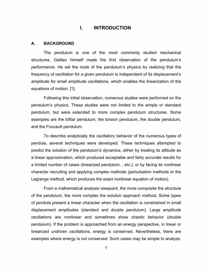
swinging is the Blackburn pendulum. [1].
Figure 1. The Blackburn pendulum
The Blackburn pendulum’s suspension system is comprised of two strings
forming a ‘’Y’’ shape. The purpose of this design is to provide two distinct and
effective pendulum string lengths. Therefore, for an oscillatory motion within a
A
B
C
3
plane defined by the Y shape, the length of the pendulum is the distance from
point B to point C. In contrast, for a motion within a plane perpendicular to the Y
shape, the effective length is the distance from point A to point C. Therefore, two
distinct frequencies of oscillation define the motion of the Blackburn pendulum in
the two perpendicular planes. Thus, its modes of oscillation are described by
superposition of the two basic frequencies.
Nevertheless, all the previously mentioned characteristics of the Blackburn
pendulum depend on the assumption that point B will not be able to oscillate with
respect to one of the two strings that starts from B and ends at the support
points, i.e., the distance of B from the two support points will always be constant.
However, this assumption is valid under restrictions. A violent motion of the
support would theoretically be able to disturb the partial equilibrium of the ‘’Y’’
pendulum.
The motivation for this thesis was to obtain analytical expressions, as well
as numerical solutions, to describe the behavior of oscillating pendula with
designs similar to the one of the ‘’Y’’ pendulum. The basic model design that will
be initially analyzed is the one of a Blackburn pendulum in which point A
coincides with B, and is allowed to oscillate only within the plane defined by this
“V’’ shape (more detailed description will be provided in the following sections).
Moreover, since such a ‘’V’’ design is the basic element component of more
complex suspension designs, its capability of preventing or damping oscillations
will be investigated.

4
THIS PAGE INTENTIONALLY LEFT BLANK
5
II. THE TWO-STRING PENDULUM
A. MATHEMATICAL DESCRIPTION OF THE TWO-STRING PENDULUM
1. Introduction
The purpose of this section is to analyze the motion equations of the two-
string pendulum. For brevity within this thesis, this will be referred to as the 2-
pendulum. Several techniques will be used to analyze the motion of the 2-
pendulum with the aim to present an accurate solution to the nonlinear equations
of motion that describes its motion. The main purpose is to compare main
features of the dynamic response of the 2-pendulum with those of the standard
single-mass, single-string pendulum. These comparisons will be in terms of the
amplitude of the resulting motion, the resulting natural frequency of the oscillator,
as well as the string tension. Different values of initial velocity and initial angular
displacement will be used to investigate the system’s response to both an initial
excitation and an initial displacement from its equilibrium position.
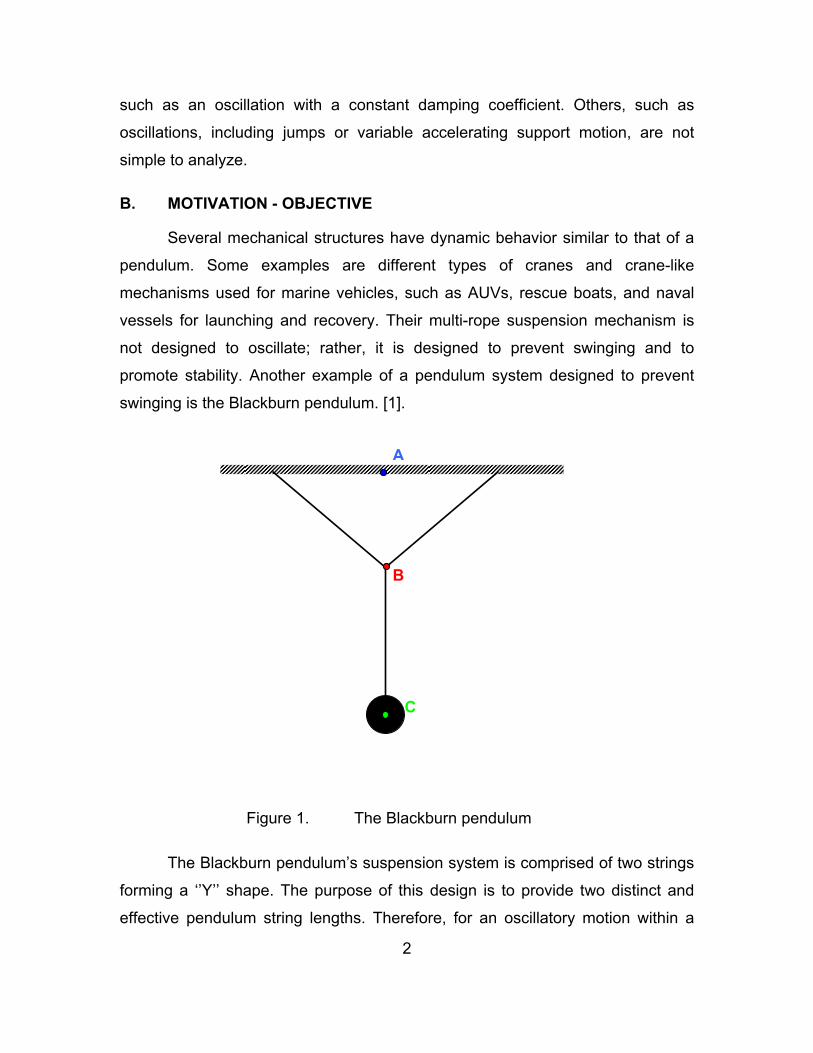
2. The Standard Pendulum
Figure 2. Small angle oscillation of the standard pendulum
θ
6
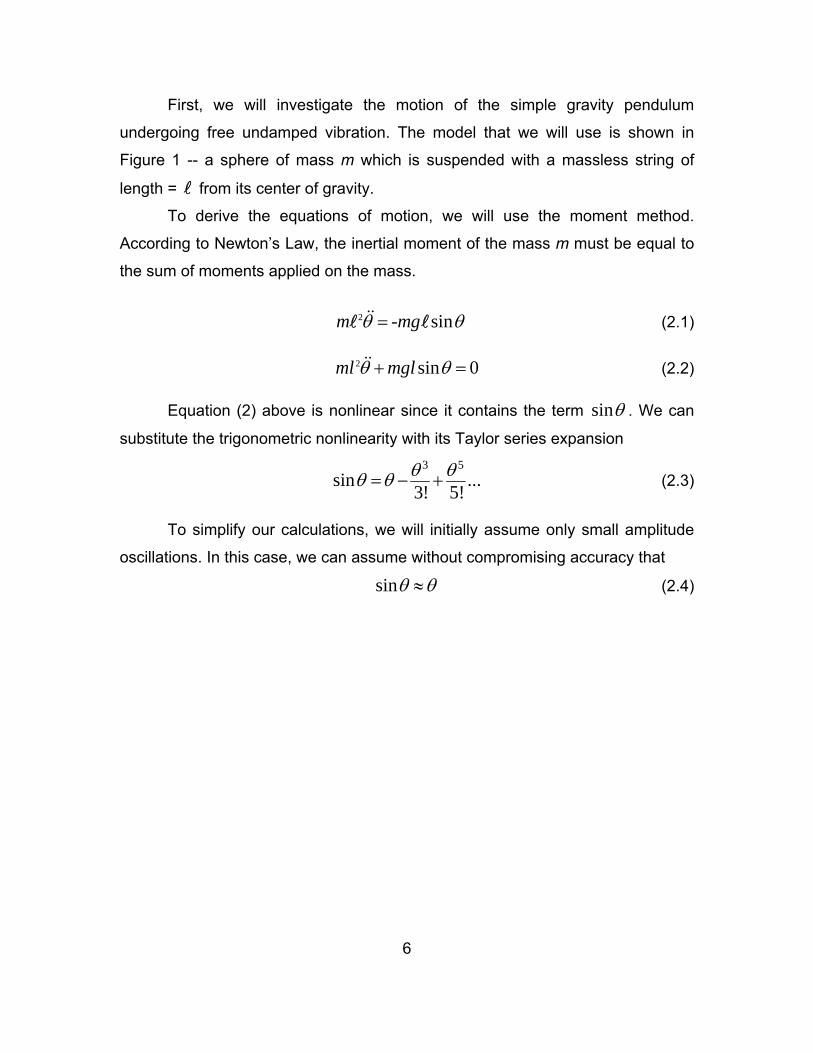
First, we will investigate the motion of the simple gravity pendulum
undergoing free undamped vibration. The model that we will use is shown in
Figure 1 -- a sphere of mass m which is suspended with a massless string of
length = from its center of gravity.
To derive the equations of motion, we will use the moment method.
According to Newton’s Law, the inertial moment of the mass m must be equal to
the sum of moments applied on the mass.
2 - sinm mgθ θ= (2.1) 2 sin 0ml mglθ θ+ = (2.2)
Equation (2) above is nonlinear since it contains the term sinθ . We can
substitute the trigonometric nonlinearity with its Taylor series expansion
3 5
sin ...3! 5!θ θθ θ= − + (2.3)
To simplify our calculations, we will initially assume only small amplitude
oscillations. In this case, we can assume without compromising accuracy that
sinθ θ≈ (2.4)
7
0 10 20 30 40 50 60 70 80 900
0.5
1
1.5
θ (degrees)
y=sin(θ)y=θ
0 10 20 30 40 50 60 70 80 90
-0.5
-0.4
-0.3
-0.2
-0.1
0
θ (degrees)
y=si
n(θ)
- θ
X: 18Y: -0.005142
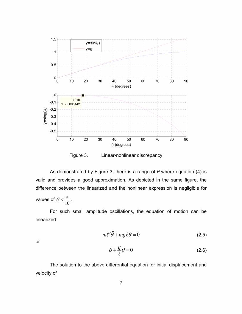
Figure 3. Linear-nonlinear discrepancy
As demonstrated by Figure 3, there is a range of θ where equation (4) is
valid and provides a good approximation. As depicted in the same figure, the
difference between the linearized and the nonlinear expression is negligible for
values of 10πθ < .
For such small amplitude oscillations, the equation of motion can be
linearized
2 0m mgθ θ+ = (2.5) or
0gθ θ+ = (2.6)
The solution to the above differential equation for initial displacement and
velocity of
8
0
0(0)(0)
θ θ
θ θ
=
= (2.7)
becomes
( ) ( )0 sin 0 cosn nn
t tθθ ω θ ωω
= + (2.8)
where ngω = (2.9)
is the natural frequency of the linear pendulum.
From Figure 2, the restoring moment is
sinrF mg θ= (2.10) or, for small oscillations,
θ=rF mg (2.11)
Another feature of the pendulum worth mentioning is the pendulum jump
[5]. Pendulum jumps occur when the mass leaves the circular path defined by the
string and follows other trajectories. Such response is only observed if the string
tension becomes zero. This is dependent on the position of the pendulum and
the initial conditions. From Figure 2, we can visualize that the centripetal force,
which obliges the mass to follow a circular path, is
2 2
cos cosmu muFc T mg T mgθ θ= = − ⇔ = + (2.12)
where u is the linear velocity of the mass. The magnitude of u depends only on
the initial conditions, since only conservative forces govern the pendulum’s
motion. Assuming the initial conditions (2.7), which are equivalent to
0 0(1 cos )z θ= − and 0 0u lθ= , the initial energy of the mass is
20 0 0 0 0
12
E T V mu mgz= + = + . During oscillation, the energy of the mass for an
9
arbitrary angle θ would be 212
E T V mu mgz= + = + , where (1 cos )z θ= − .
Since the total energy is conserved throughout the oscillation (absence of
damping or other non-conservative forces) 0E E= , the magnitude of the linear
velocity would be
02= −Eu gzm
(2.13)
Finally, the tension of the string throughout the oscillation, from (2.12) and
(2.13), will be equal to
02( ) cosθ−= +
E mgzT mg (2.14)
where a positive sign denotes orientation towards the center of oscillation. This
promotes the circular path motion of the mass. The only term of the latest
equation that may take negative values and, thus, lead to zeroing the string
tension, is cosmg θ . It may only happen for angular displacements greater than
π2
.
The possibility of jumps is present only if the initial conditions allow the
oscillator to climb to 2πθ > . After that point, the path of the mass would be
governed by the regular equations which define a projectile with a given initial
linear velocity magnitude and orientation; that is, until the position of the mass
will again reach a distance equal to the natural length of the pendulum’s string.
10
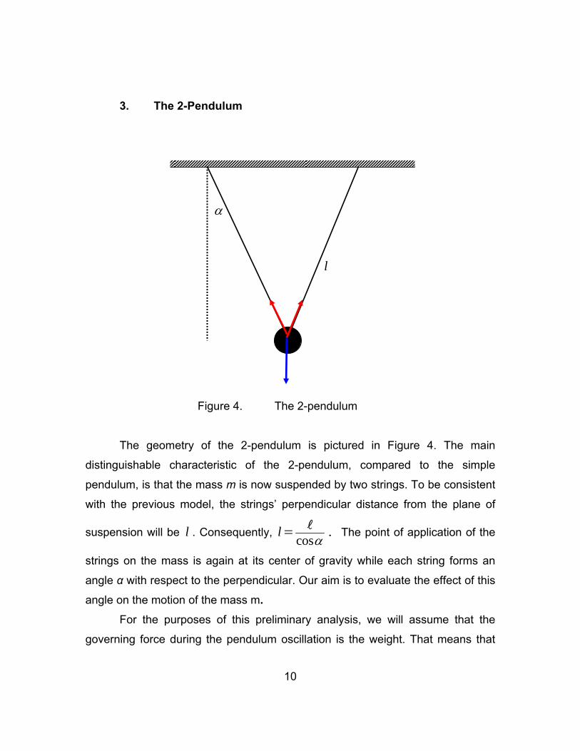
3. The 2-Pendulum
Figure 4. The 2-pendulum
The geometry of the 2-pendulum is pictured in Figure 4. The main
distinguishable characteristic of the 2-pendulum, compared to the simple
pendulum, is that the mass m is now suspended by two strings. To be consistent
with the previous model, the strings’ perpendicular distance from the plane of
suspension will be l . Consequently, cos
lα
= . The point of application of the
strings on the mass is again at its center of gravity while each string forms an
angle α with respect to the perpendicular. Our aim is to evaluate the effect of this
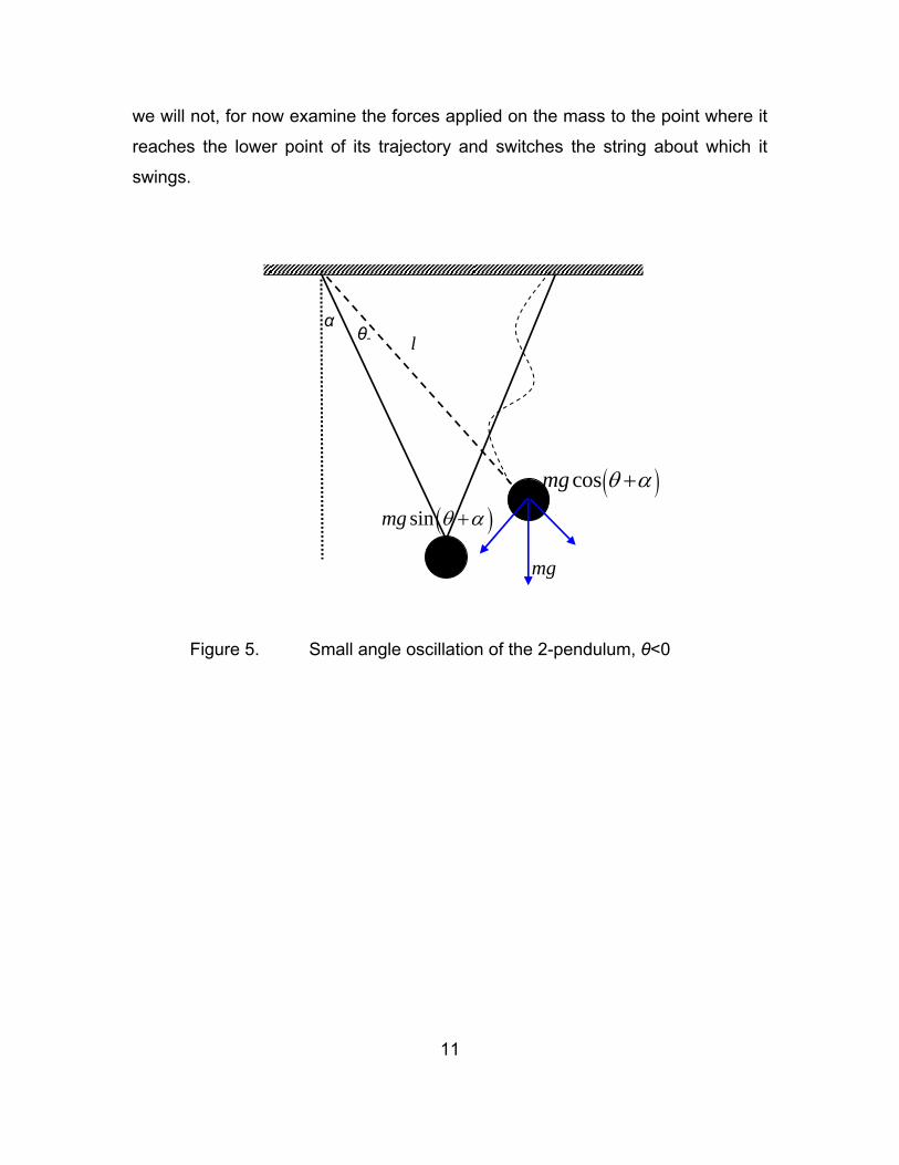
angle on the motion of the mass m. For the purposes of this preliminary analysis, we will assume that the
governing force during the pendulum oscillation is the weight. That means that
α
l
11
we will not, for now examine the forces applied on the mass to the point where it
reaches the lower point of its trajectory and switches the string about which it
swings.
Figure 5. Small angle oscillation of the 2-pendulum, θ<0
θ-α
l
mg
( )sinmg θ α+
( )cosmg θ α+
12
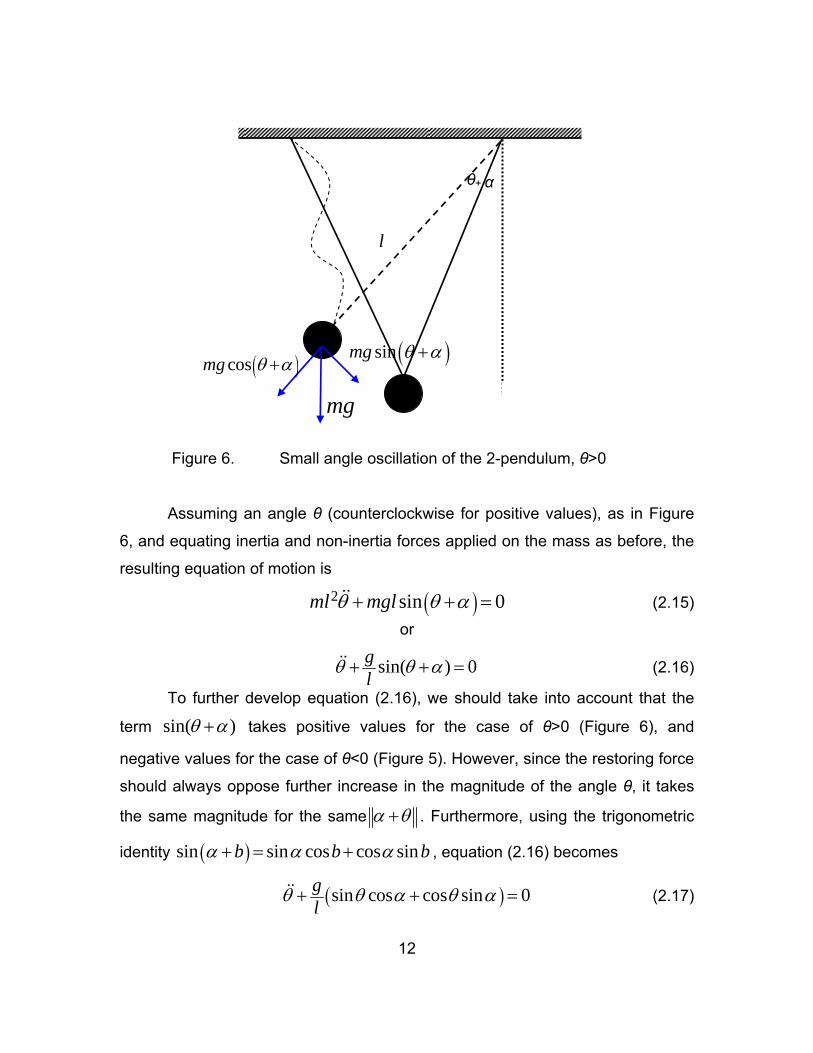
Figure 6. Small angle oscillation of the 2-pendulum, θ>0
Assuming an angle θ (counterclockwise for positive values), as in Figure
6, and equating inertia and non-inertia forces applied on the mass as before, the
resulting equation of motion is
( )2 sin 0θ θ α+ + =ml mgl (2.15)
or
sin( ) 0θ θ α+ + =gl
(2.16)
To further develop equation (2.16), we should take into account that the
term sin( )θ α+ takes positive values for the case of θ>0 (Figure 6), and
negative values for the case of θ<0 (Figure 5). However, since the restoring force
should always oppose further increase in the magnitude of the angle θ, it takes
the same magnitude for the same α θ+ . Furthermore, using the trigonometric
identity ( )sin sin cos cos sinb b bα α α+ = + , equation (2.16) becomes
( )sin cos cos sin 0θ θ α θ α+ + =gl
(2.17)
θ+ α
l
mg
( )sinmg θ α+( )cosmg θ α+
13
Examining equation (2.17), we can see that the consistency of the
restoring force orientation is preserved in the term sin cosθ α (because of
sinθ ), but not in sin cosα θ (since cosθ does not change sign when θ changes
sign). Consequently, to preserve the restoring force consistency for all values of
θ, we should rewrite equation (2.17) as follows
sin cos cos sin 0g gl l
θ θ α θ α+ ± =
This is equivalent to
sin cos cos sin sign 0θ θ α θ α θ+ + =g gl l
(2.18)
The sign nonlinearity assumes the value (+1) for positive and (-1) for
negative arguments. In addition to the above, if we assume small angles of θ, we
can rewrite (2.18) as follows
cos sin sign 0θ θ α α θ+ + =g gl l
(2.19)
The restoring force from equation (2.15) is
sin( )θ α= +rF mg (2.20) For small oscillations, equation (2.20) becomes
cos sin signθ α α θ= +rF mg mg (2.21) Our goal is to solve analytically and numerically differential equations
(2.18).
Finally, based on the previous analysis performed on the jumps for the
standard pendulum, we realize that the 2-pendulum may exhibit the same
behavior, only now the required angular displacement is2 2π πθ α θ α+ > ⇔ > − .
4. Comments
Despite its similarity with the standard pendulum, equation (2.18) exhibits
some major characteristic differences. The most significant difference between
the standard pendulum and the 2-pendulum is that the latter possesses a
14
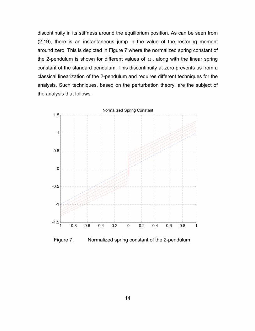
discontinuity in its stiffness around the equilibrium position. As can be seen from
(2.19), there is an instantaneous jump in the value of the restoring moment
around zero. This is depicted in Figure 7 where the normalized spring constant of
the 2-pendulum is shown for different values of α , along with the linear spring
constant of the standard pendulum. This discontinuity at zero prevents us from a
classical linearization of the 2-pendulum and requires different techniques for the
analysis. Such techniques, based on the perturbation theory, are the subject of
the analysis that follows.
-1 -0.8 -0.6 -0.4 -0.2 0 0.2 0.4 0.6 0.8 1-1.5
-1
-0.5
0
0.5
1
1.5Normalized Spring Constant
Figure 7. Normalized spring constant of the 2-pendulum
15
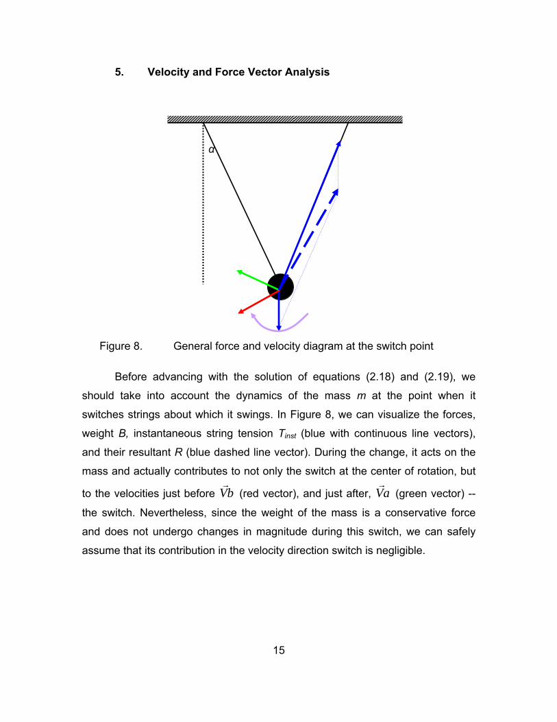
5. Velocity and Force Vector Analysis
Figure 8. General force and velocity diagram at the switch point
Before advancing with the solution of equations (2.18) and (2.19), we
should take into account the dynamics of the mass m at the point when it
switches strings about which it swings. In Figure 8, we can visualize the forces,
weight B, instantaneous string tension Τinst (blue with continuous line vectors),
and their resultant R (blue dashed line vector). During the change, it acts on the
mass and actually contributes to not only the switch at the center of rotation, but
to the velocities just before Vb (red vector), and just after, Va (green vector) --
the switch. Nevertheless, since the weight of the mass is a conservative force
and does not undergo changes in magnitude during this switch, we can safely
assume that its contribution in the velocity direction switch is negligible.
α
16
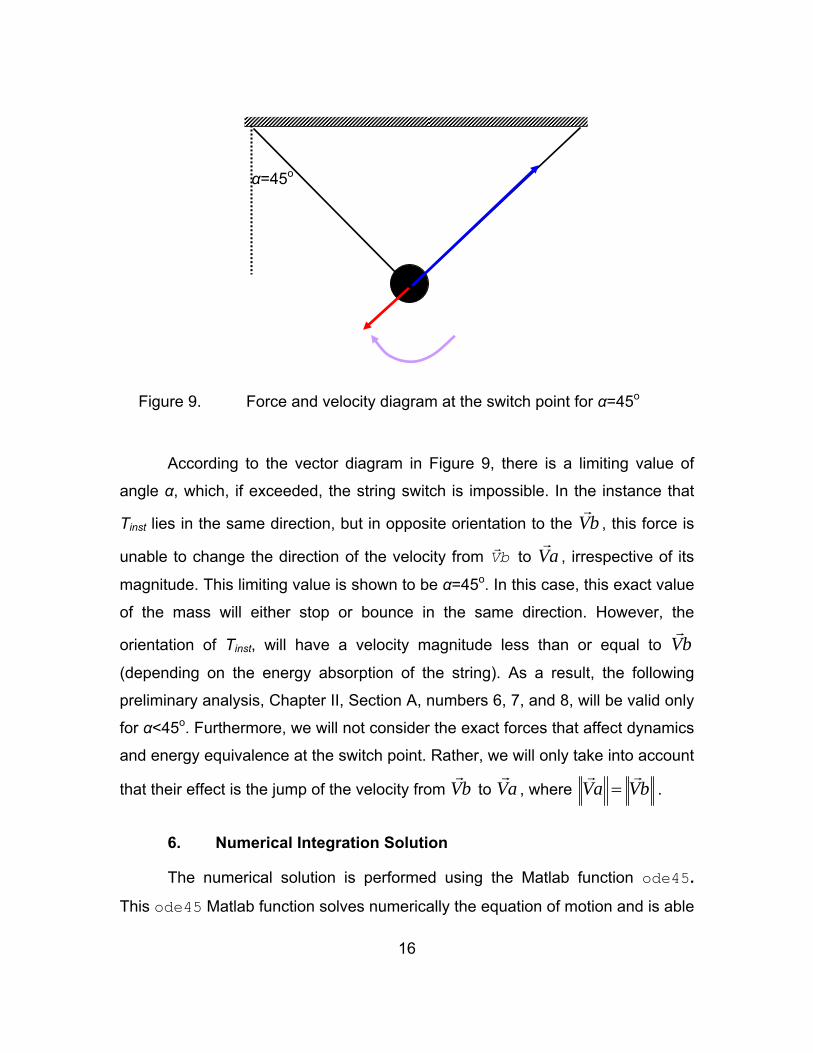
Figure 9. Force and velocity diagram at the switch point for α=45o
According to the vector diagram in Figure 9, there is a limiting value of
angle α, which, if exceeded, the string switch is impossible. In the instance that
Tinst lies in the same direction, but in opposite orientation to the Vb , this force is
unable to change the direction of the velocity from Vb to Va , irrespective of its
magnitude. This limiting value is shown to be α=45o. In this case, this exact value
of the mass will either stop or bounce in the same direction. However, the
orientation of Tinst, will have a velocity magnitude less than or equal to Vb
(depending on the energy absorption of the string). As a result, the following
preliminary analysis, Chapter II, Section A, numbers 6, 7, and 8, will be valid only
for α<45o. Furthermore, we will not consider the exact forces that affect dynamics
and energy equivalence at the switch point. Rather, we will only take into account
that their effect is the jump of the velocity from Vb to Va , where Va Vb= .
6. Numerical Integration Solution
The numerical solution is performed using the Matlab function ode45.
This ode45 Matlab function solves numerically the equation of motion and is able
α=45o
17
to take into account nonlinearities, such as trigonometric functions and sign
changes. Thus, ode45 will provide the exact solution, provided that an
appropriate, fine enough, time step is selected. The Program_1.m Matlab-file was used to plot the angular displacement θ versus time for different values of
angle α, assuming initial conditions 0(0)θ θ= and (0) 0θ = . In parallel, we
plotted the angular displacement θ versus time for a simple pendulum of string
length . In addition, the Program_2.m provided the same kind of plots, where
the initial conditions were (0) 0θ = and 0(0)θ θ= .
7. Analytical Solution
Three different methods will be used to attempt to derive the exact or
approximate solution to equation (14) or its equivalent (16).
a. Exact Solution for a Time Increment
One method we could use to obtain the solution of equation (2.18)
is to solve it for the time period where the term sin signgl
α θ has a constant
sign [2]. Thus, assuming an initial angular displacement θ(0)=Α, the equation of
motion for 0<θ<Α is
sin sin
cos coscos cos
α αθ α
α α
⎛ ⎞⎜ ⎟ ⎛ ⎞
⎜ ⎟⎜ ⎟ ⎜ ⎟⎝ ⎠⎜ ⎟
⎝ ⎠
= − + +g g
gl lA tg g ll l
(2.22)
or
( )tan tan cos cosθ α α α⎛ ⎞⎜ ⎟⎜ ⎟⎝ ⎠
= − + + gA tl
(2.23)
Let us name the square of the pseudo-natural frequency of
oscillation and of the equivalent pseudo-forcing amplitude as bellow
20 cos
sin
ω α
α
=
=
gl
gPl
(2.24)
18
At the time 1 20 0
1 1arccos1
tAP
ω ω
⎛ ⎞⎜ ⎟⎜ ⎟⎜ ⎟⎜ ⎟⎝ ⎠
=+
when θ=0, the velocity is
( ) 01 0 20
sinPu t A tω ωω
⎛ ⎞⎜ ⎟⎜ ⎟⎝ ⎠
= − +
and then the equation of motion becomes
20θ ω θ+ = P (2.25)
with initial conditions ( ) 01 0 20
sinPu t A tω ωω
⎛ ⎞⎜ ⎟⎜ ⎟⎝ ⎠
= − + and ( )1 0tθ = , and so on. The
value 1t is equivalent to one quarter of the period of oscillation.
Finally the period of oscillation is
20 0
4 1arccos1ω ω
⎛ ⎞⎜ ⎟⎜ ⎟⎜ ⎟⎜ ⎟⎝ ⎠
=+
exactTAP
(2.26)
or
4 1arccos1cos tanα α
⎛ ⎞⎜ ⎟⎜ ⎟⎜ ⎟⎜ ⎟⎝ ⎠
=+exactT Ag
l
(2.27)
so the frequency of oscillation is
2πω =exactexactT
(2.28)
b. Method of Slowly Changing Phase and Amplitude
A second method for obtaining the analytic solution only for the
linearized equation (2.19) or , considering (2.24)
20 sign 0θ ω θ θ+ + =P , (2.29)
19
is using the method of Slowly Changing Phase and Amplitude [2]. This method
states that the equations of the slowly changing phase ψ and amplitude a are
( ) ( ){ } ( )20
0
1 - a sin sin a2 a
πψ θ ψ ψ θπ ω
⎡ ⎤⎣ ⎦= + +∫ P d (2.30)
( ) ( ){ } ( )2
00
1a - a sin sin a a2 a
π θ ψ ψπ ω
⎡ ⎤⎣ ⎦= + +∫ Psign d (2.31)
Evaluating the above integrals,
a 0= and 0
42 a
Pψπ ω
=
a A= and 00
2PA
ψ ψπ ω
= +
Finally, if we choose the initial conditions, such as 0 2πψ = , the approximate
solution is
00
2cosθ ωπ ω
⎛ ⎞⎜ ⎟⎜ ⎟⎝ ⎠
= Α + P tA
(2.32)
and the approximate period is
0 20
221
π
ωπω
⎛ ⎞⎜ ⎟⎜ ⎟⎝ ⎠
=
+appT
PA
(2.33)
while the approximate angular frequency is
0 20
21ω ωπω
⎛ ⎞⎜ ⎟⎜ ⎟⎝ ⎠
= +appP
A (2.34)
considering (2.24)
2tancos 1 αω απ
⎛ ⎞⎜ ⎟⎝ ⎠
= +appgl A
(2.35)
c. Energy Method
The application of this method suggests that we could approximate
the equation of motion of the enhanced pendulum with one of a simple
pendulum. However, the restoring force would be increased by a factor so that
20
the total work produced by this force along a time period would be the same as
the forces that govern the motion of the enhanced pendulum.
From equation (2.20), the work produced by the restoring force of
the enhanced pendulum for a motion 0<θ <θ0 is equal to
( )00 sinθ α θ θ+∫ mg d (2.36)
while the one of the simple pendulum is
00 sinθ θ θ∫ mg d (2.37)
Dividing (2.36) by (2.37), we obtain a factor of
( )0 00 0/sin sinθ θα θ θ θ θ= +∫ ∫F mg d mg d (2.38)
which provides us with an order of increased magnitude of forces applied during
the oscillation of the enhanced pendulum compared to the ones applied on the
simple pendulum.
Thus, we will multiply the term sinθmg by F and solve the
approximate equation of motion
sin 0θ θ+ =gFl
(2.39)
or in linear form,
0θ θ+ =gFl
(2.40)
Thus, the approximate angular frequency of oscillation is
ω =appg Fl
(2.41)
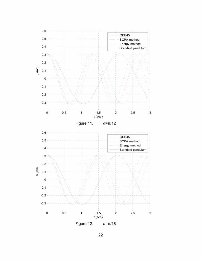
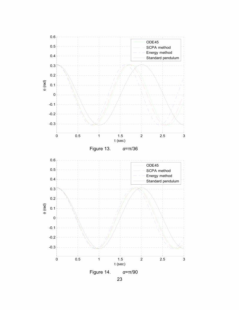
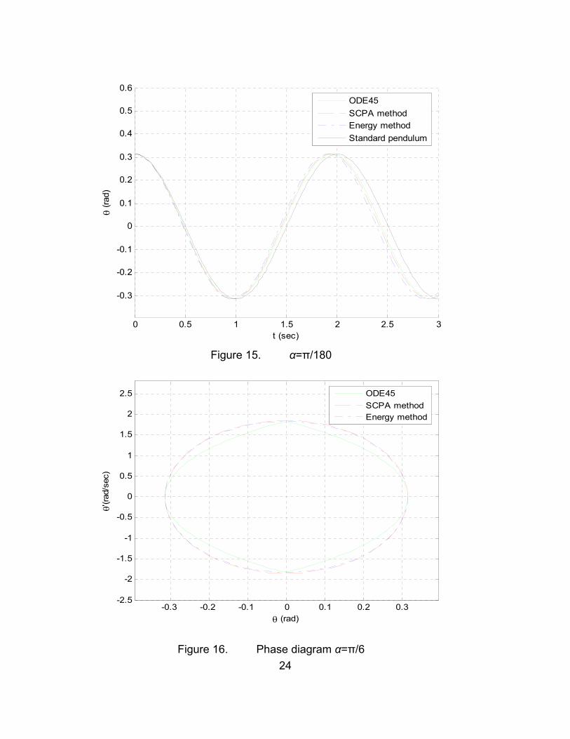
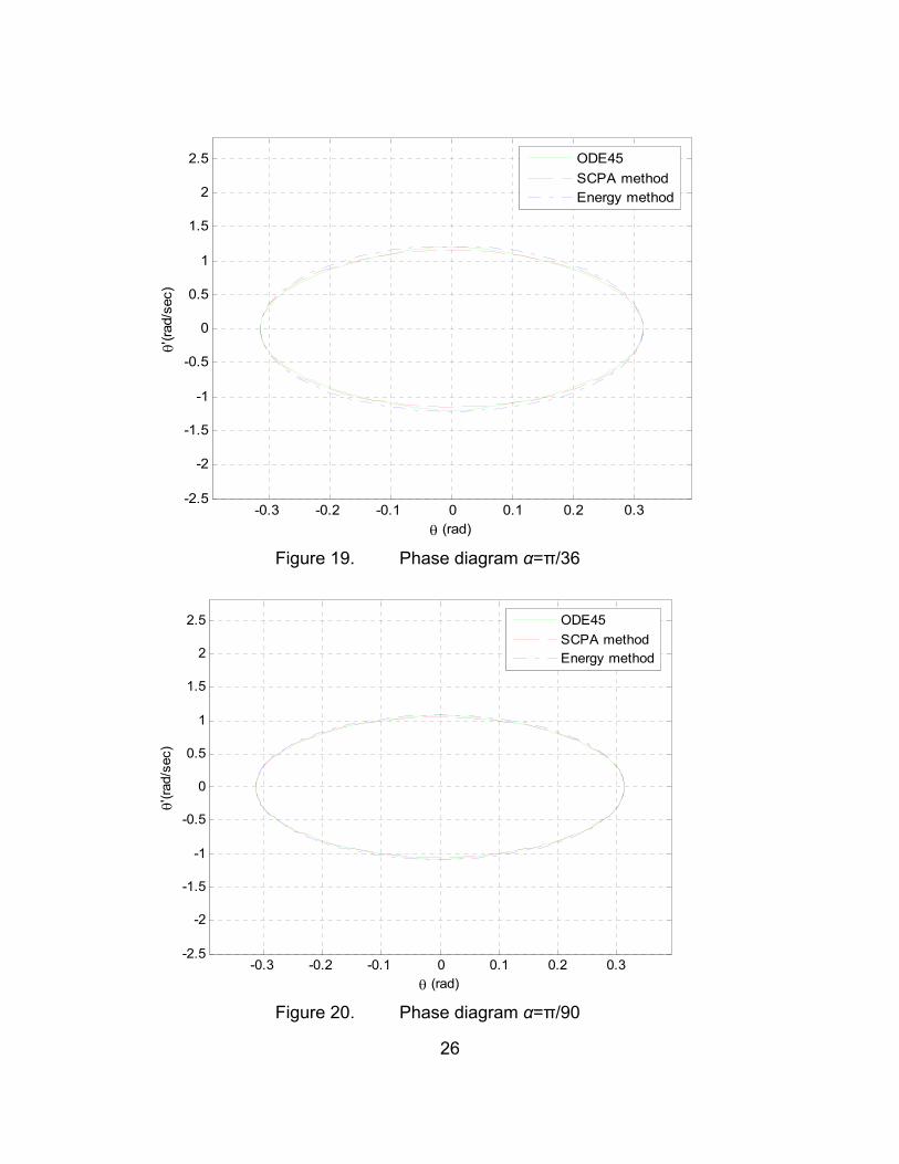
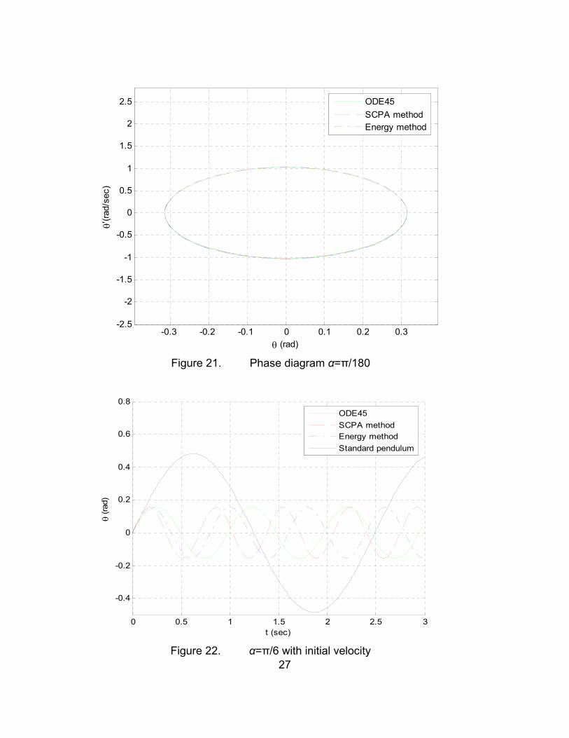
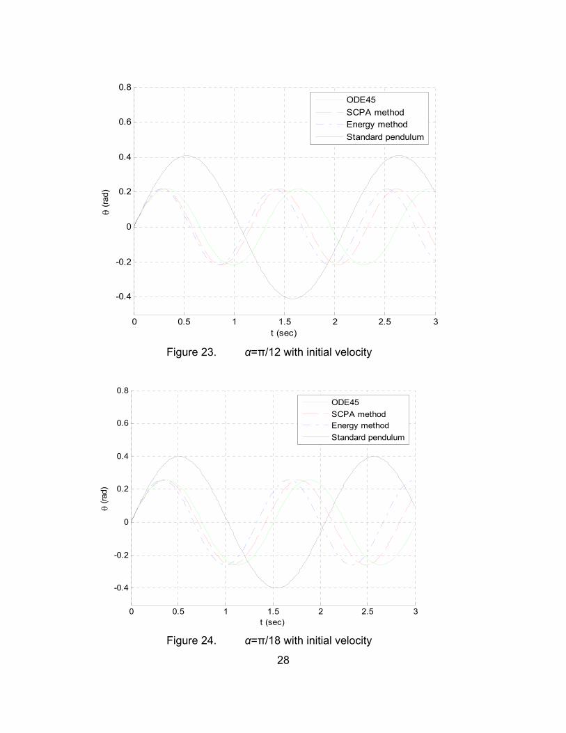
8. Evaluation of Results
To evaluate both numerical and analytical approximations, we will first plot
the three angular displacement solutions (ode45 numerical integration – Slowly
Changing Phase and Amplitude method – Energy method). This will be
compared to the solution of the standard pendulum in terms of gain and
frequency of oscillation. This will best show that the 2-pendulum offers significant
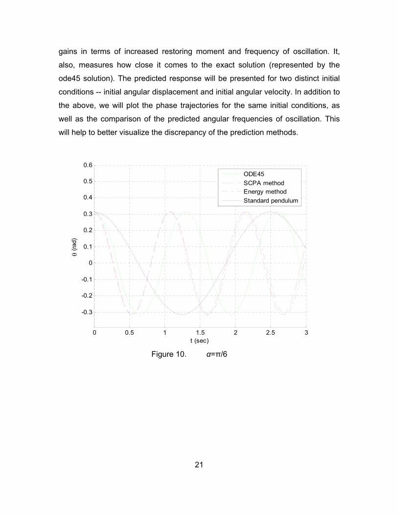
21
gains in terms of increased restoring moment and frequency of oscillation. It,
also, measures how close it comes to the exact solution (represented by the
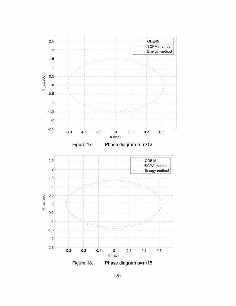
ode45 solution). The predicted response will be presented for two distinct initial
conditions -- initial angular displacement and initial angular velocity. In addition to
the above, we will plot the phase trajectories for the same initial conditions, as
well as the comparison of the predicted angular frequencies of oscillation. This
will help to better visualize the discrepancy of the prediction methods.
0 0.5 1 1.5 2 2.5 3
-0.3
-0.2
-0.1
0
0.1
0.2
0.3
0.4
0.5
0.6
t (sec)
θ (ra
d)
ODE45SCPA methodEnergy methodStandard pendulum
Figure 10. α=π/6
22
0 0.5 1 1.5 2 2.5 3
-0.3
-0.2
-0.1
0
0.1
0.2
0.3
0.4
0.5
0.6
t (sec)
θ (ra
d)ODE45SCPA methodEnergy methodStandard pendulum
Figure 11. α=π/12
0 0.5 1 1.5 2 2.5 3
-0.3
-0.2
-0.1
0
0.1
0.2
0.3
0.4
0.5
0.6
t (sec)
θ (r
ad)
ODE45SCPA methodEnergy methodStandard pendulum
Figure 12. α=π/18
23
0 0.5 1 1.5 2 2.5 3
-0.3
-0.2
-0.1
0
0.1
0.2
0.3
0.4
0.5
0.6
t (sec)
θ (ra
d)ODE45SCPA methodEnergy methodStandard pendulum
Figure 13. α=π/36
0 0.5 1 1.5 2 2.5 3
-0.3
-0.2
-0.1
0
0.1
0.2
0.3
0.4
0.5
0.6
t (sec)
θ (ra
d)
ODE45SCPA methodEnergy methodStandard pendulum
Figure 14. α=π/90
24
0 0.5 1 1.5 2 2.5 3
-0.3
-0.2
-0.1
0
0.1
0.2
0.3
0.4
0.5
0.6
t (sec)
θ (r
ad)
ODE45SCPA methodEnergy methodStandard pendulum
Figure 15. α=π/180
-0.3 -0.2 -0.1 0 0.1 0.2 0.3-2.5
-2
-1.5
-1
-0.5
0
0.5
1
1.5
2
2.5
θ (rad)
θ'(ra
d/se
c)
ODE45SCPA methodEnergy method
Figure 16. Phase diagram α=π/6
25
-0.3 -0.2 -0.1 0 0.1 0.2 0.3-2.5
-2
-1.5
-1
-0.5
0
0.5
1
1.5
2
2.5
θ (rad)
θ'(ra
d/se
c)ODE45SCPA methodEnergy method
Figure 17. Phase diagram α=π/12
-0.3 -0.2 -0.1 0 0.1 0.2 0.3-2.5
-2
-1.5
-1
-0.5
0
0.5
1
1.5
2
2.5
θ (rad)
θ'(ra
d/se
c)
ODE45SCPA methodEnergy method
Figure 18. Phase diagram α=π/18
26
-0.3 -0.2 -0.1 0 0.1 0.2 0.3-2.5
-2
-1.5
-1
-0.5
0
0.5
1
1.5
2
2.5
θ (rad)
θ'(ra
d/se
c)ODE45SCPA methodEnergy method
Figure 19. Phase diagram α=π/36
-0.3 -0.2 -0.1 0 0.1 0.2 0.3-2.5
-2
-1.5
-1
-0.5
0
0.5
1
1.5
2
2.5
θ (rad)
θ'(ra
d/se
c)
ODE45SCPA methodEnergy method
Figure 20. Phase diagram α=π/90
27
-0.3 -0.2 -0.1 0 0.1 0.2 0.3-2.5
-2
-1.5
-1
-0.5
0
0.5
1
1.5
2
2.5
θ (rad)
θ'(ra
d/se
c)ODE45SCPA methodEnergy method
Figure 21. Phase diagram α=π/180
0 0.5 1 1.5 2 2.5 3
-0.4
-0.2
0
0.2
0.4
0.6
0.8
t (sec)
θ (ra
d)
ODE45SCPA methodEnergy methodStandard pendulum
Figure 22. α=π/6 with initial velocity
28
0 0.5 1 1.5 2 2.5 3
-0.4
-0.2
0
0.2
0.4
0.6
0.8
t (sec)
θ (ra
d)ODE45SCPA methodEnergy methodStandard pendulum
Figure 23. α=π/12 with initial velocity
0 0.5 1 1.5 2 2.5 3
-0.4
-0.2
0
0.2
0.4
0.6
0.8
t (sec)
θ (ra
d)
ODE45SCPA methodEnergy methodStandard pendulum
Figure 24. α=π/18 with initial velocity

29
0 0.5 1 1.5 2 2.5 3
-0.4
-0.2
0
0.2
0.4
0.6
0.8
t (sec)
θ (ra
d)ODE45SCPA methodEnergy methodStandard pendulum
Figure 25. α=π/36 with initial velocity
0 0.5 1 1.5 2 2.5 3
-0.4
-0.2
0
0.2
0.4
0.6
0.8
t (sec)
θ (ra
d)
ODE45SCPA methodEnergy methodStandard pendulum
Figure 26. α=π/90 with initial velocity
30
0 0.5 1 1.5 2 2.5 3
-0.4
-0.2
0
0.2
0.4
0.6
0.8
t (sec)
θ (ra
d)ODE45SCPA methodEnergy methodStandard pendulum
Figure 27. α=π/180 with initial velocity
0 5 10 15 20 25 30 35 40 450
2
4
6
8
10
12
14
16
a (degrees)
ω (r
ad/s
ec)
Exact solutionSCPA methodEnergy methodStandard pendulum
Figure 28. θ0=π/6
31
0 5 10 15 20 25 30 35 40 450
2
4
6
8
10
12
14
16
a (degrees)
ω (r
ad/s
ec)
Exact solutionSCPA methodEnergy methodStandard pendulum
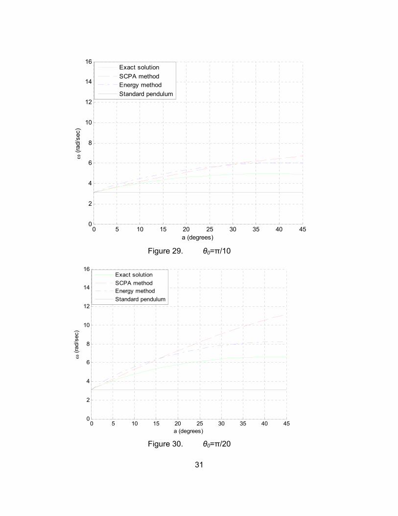
Figure 29. θ0=π/10
0 5 10 15 20 25 30 35 40 450
2
4
6
8
10
12
14
16
a (degrees)
ω (r
ad/s
ec)
Exact solutionSCPA methodEnergy methodStandard pendulum
Figure 30. θ0=π/20
32
0 5 10 15 20 25 30 35 40 450
2
4
6
8
10
12
14
16
a (degrees)
ω (r
ad/s
ec)
Exact solutionSCPA methodEnergy methodStandard pendulum
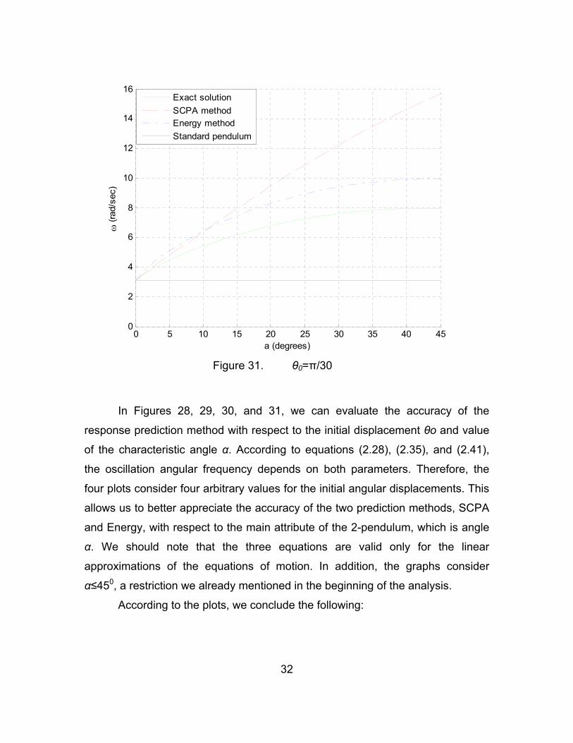
Figure 31. θ0=π/30
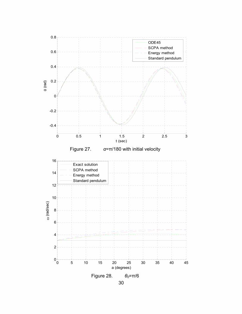
In Figures 28, 29, 30, and 31, we can evaluate the accuracy of the
response prediction method with respect to the initial displacement θο and value
of the characteristic angle α. According to equations (2.28), (2.35), and (2.41),
the oscillation angular frequency depends on both parameters. Therefore, the
four plots consider four arbitrary values for the initial angular displacements. This
allows us to better appreciate the accuracy of the two prediction methods, SCPA
and Energy, with respect to the main attribute of the 2-pendulum, which is angle
α. We should note that the three equations are valid only for the linear
approximations of the equations of motion. In addition, the graphs consider
α≤450, a restriction we already mentioned in the beginning of the analysis.
According to the plots, we conclude the following:
33
• The angular frequency ω of the 2-pendulum is greater compared to
the frequency of the standard pendulum which has the same equivalent string
length .
• A smaller maximum angular displacement for the 2-pendulum
compared to the standard pendulum results from applying the same initial
angular velocity.
• The discrepancy between the two predictions, and the exact
calculations, is very low for small values of α, but increases for larger ones. More
specifically, while the Energy method follows the exact solution slope trend
(although providing higher predicted values), the SCPA method increases almost
linearly.
• The SCPA method tends to provide more accurate predictions for
larger values of θ0. If θ0 becomes too small, the discrepancy from the exact
solution grows and, therefore, the predictions are incorrect.
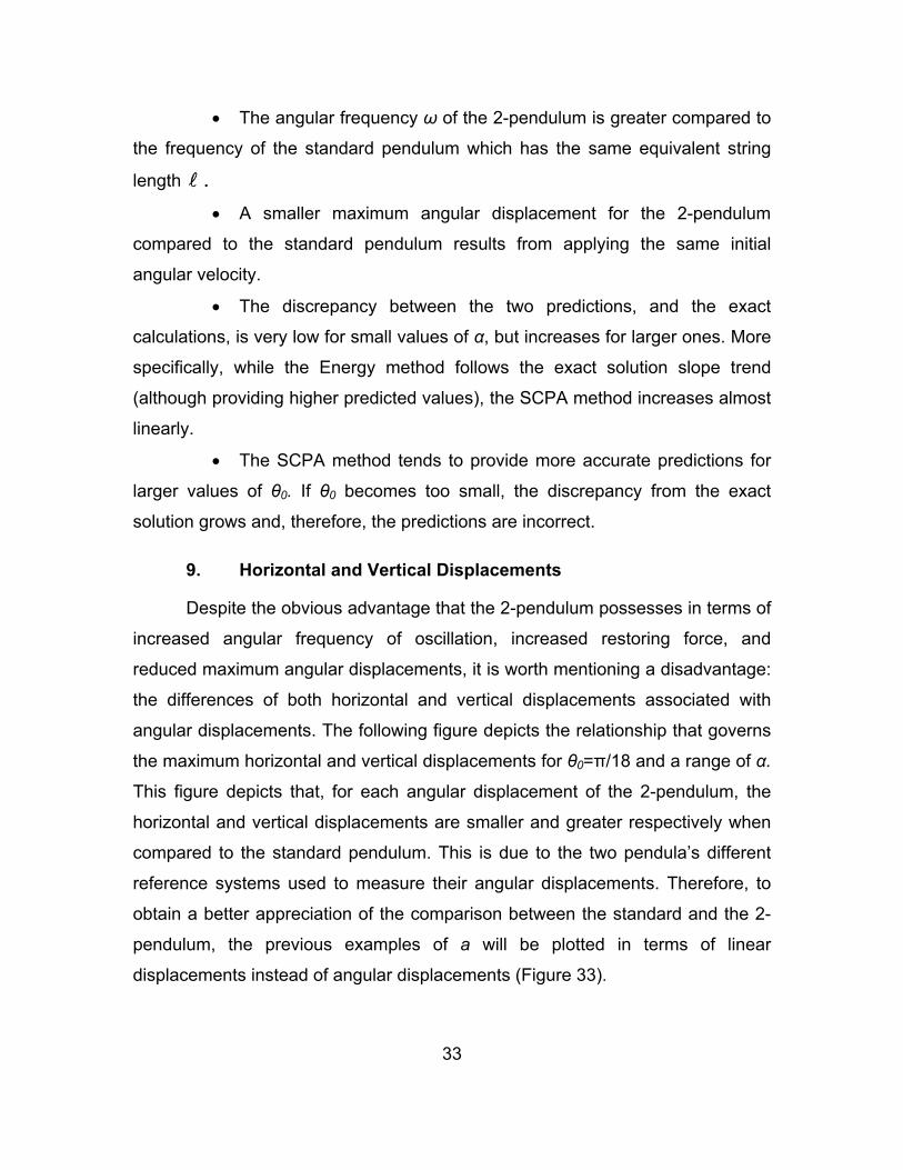
9. Horizontal and Vertical Displacements
Despite the obvious advantage that the 2-pendulum possesses in terms of
increased angular frequency of oscillation, increased restoring force, and
reduced maximum angular displacements, it is worth mentioning a disadvantage:
the differences of both horizontal and vertical displacements associated with
angular displacements. The following figure depicts the relationship that governs
the maximum horizontal and vertical displacements for θ0=π/18 and a range of α.
This figure depicts that, for each angular displacement of the 2-pendulum, the
horizontal and vertical displacements are smaller and greater respectively when
compared to the standard pendulum. This is due to the two pendula’s different
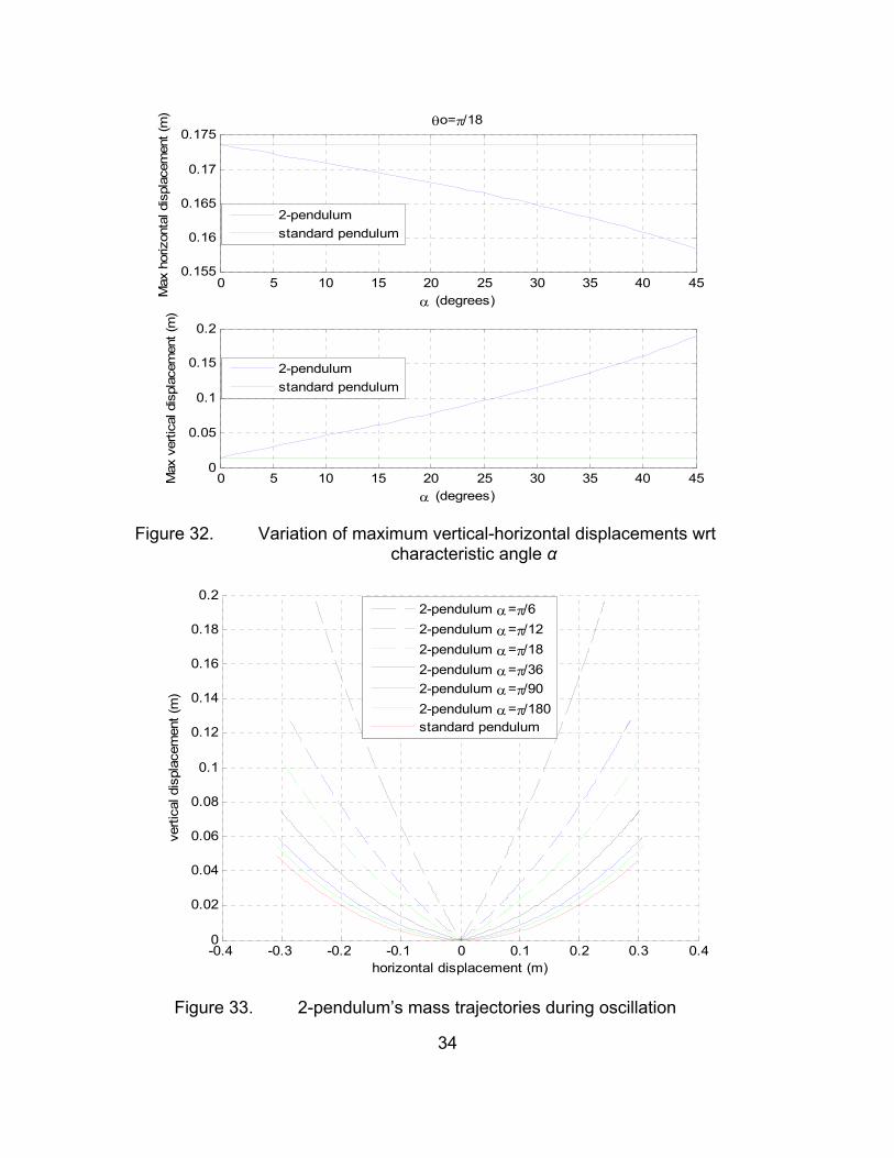
reference systems used to measure their angular displacements. Therefore, to
obtain a better appreciation of the comparison between the standard and the 2-
pendulum, the previous examples of a will be plotted in terms of linear
displacements instead of angular displacements (Figure 33).
34
0 5 10 15 20 25 30 35 40 450.155
0.16
0.165
0.17
0.175
α (degrees)Max
hor
izon
tal d
ispl
acem
ent (
m) θo=π/18
2-pendulumstandard pendulum
0 5 10 15 20 25 30 35 40 450
0.05
0.1
0.15
0.2
α (degrees)
Max
ver
tical
dis
plac
emen
t (m
)
2-pendulumstandard pendulum
Figure 32. Variation of maximum vertical-horizontal displacements wrt
characteristic angle α
-0.4 -0.3 -0.2 -0.1 0 0.1 0.2 0.3 0.40
0.02
0.04
0.06
0.08
0.1
0.12
0.14
0.16
0.18
0.2
horizontal displacement (m)
verti
cal d
ispl
acem
ent (
m)
2-pendulum α=π/62-pendulum α=π/122-pendulum α=π/182-pendulum α=π/362-pendulum α=π/902-pendulum α=π/180standard pendulum
Figure 33. 2-pendulum’s mass trajectories during oscillation
35
B. STRING TENSION INVESTIGATION
1. Analytical Formulation
Another important concept that requires further investigation is the tension
applied on the string of the 2-pendulum. As already seen in equations (2.15) and
(2.2), the restoring moment on the mass m is larger compared to the standard
pendulum. Contrarily, the string tension has smaller values since two strings,
instead of one, are used to suspend the mass. As pictured in Figure 3, while in
equilibrium, positioning the string tension is dependant only on the value of the
characteristic angle α
2cosα
= mgTs (2.42)
According to Figure 4, during swinging and while the sign of angle θ is
continuous, the string tension can be computed as follows
( )cos α θ= + +Ts Fc mg (2.43)
where 2
2
lmuFc m lθ= = is the centripetal force.
Equation (2.43) shows that the magnitude of static Ts ranges from
2mg Ts≤ ≤∞ , for 0
2πα θ≤ + ≤ , proving that increasing the characteristic angle
does not have only positive results in the overall design.
To determine the dynamic string tension, trigonometric equalities are
applied and 2 cos cos sin sinTs m l mg mgθ α θ α θ= + −
To attempt to linearize the above equation for θ< π10
,
2 cos sinθ α θ αθ= + −Ts m l mg sign mg (2.44)
36
For the standard pendulum, the calculations are easier. Therefore, the
tension applied on the string, while in equilibrium position, is
=Ts mg (2.45) and during the oscillation is
2 cosθ θ= +Ts m l mg (2.46) or, for small amplitude oscillations,
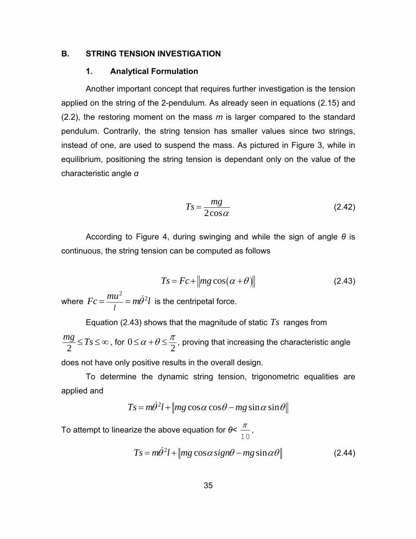
2θ= +Ts m l mg (2.47) Since ode45 solves the exact differential equation of motion and, we
already evaluated the accuracy of the predictions provided by the SCPA and
Energy methods, the string tension simulation will be performed using the results
provided by the ode45 method.
0 0.5 1 1.5 2 2.5 30
2
4
6
8
10
12
14
t (sec)
T (N
)
Figure 34. Tension for α=π/18 – θ0=π/10
37
0 5 10 15 20 25 30 35 40 450
5
10
15
20
25
30
α (degrees)
Tens
ion
(N)
Tmax θo=π/6Tmin θo=π/6Tmax θo=π/10Tmin θo=π/10Tmax θo=π/20Tmin θo=π/20
Figure 35. Maximum and minimum tensions
010
2030
40
10
20
30
40
0
5
10
15
20
θo (degrees)α (degrees)
T (N
)
Figure 36. Maximum and minimum tensions 3-D variation
38
0 5 10 15 20 25 30 35 40 45
5
10
15
20
25
30
35
40
45
θo (degrees)
α (d
egre
es)
Figure 37. Minimum tension variation
0 5 10 15 20 25 30 35 40 45
5
10
15
20
25
30
35
40
45
θo (degrees)
α (d
egre
es)
Figure 38. Maximum tension variation
39
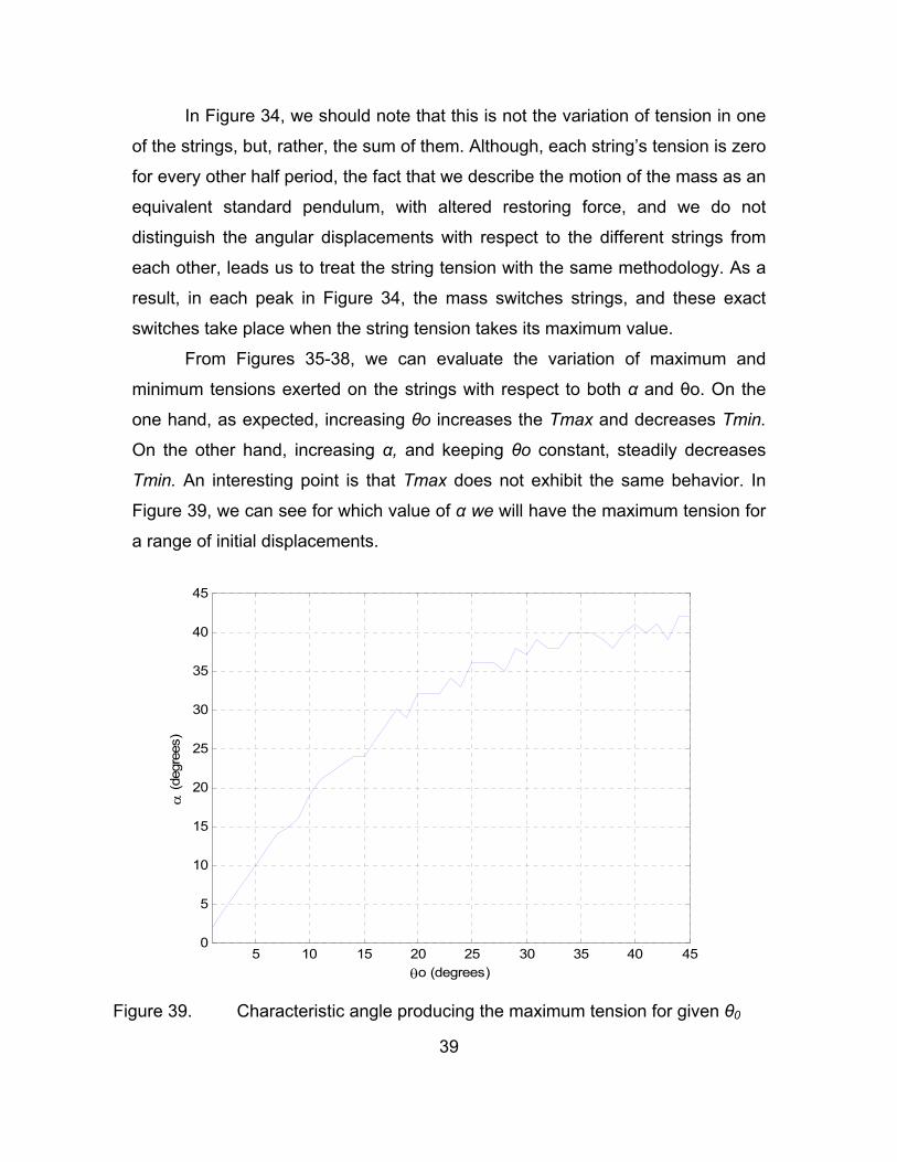
In Figure 34, we should note that this is not the variation of tension in one
of the strings, but, rather, the sum of them. Although, each string’s tension is zero
for every other half period, the fact that we describe the motion of the mass as an
equivalent standard pendulum, with altered restoring force, and we do not
distinguish the angular displacements with respect to the different strings from
each other, leads us to treat the string tension with the same methodology. As a
result, in each peak in Figure 34, the mass switches strings, and these exact
switches take place when the string tension takes its maximum value.
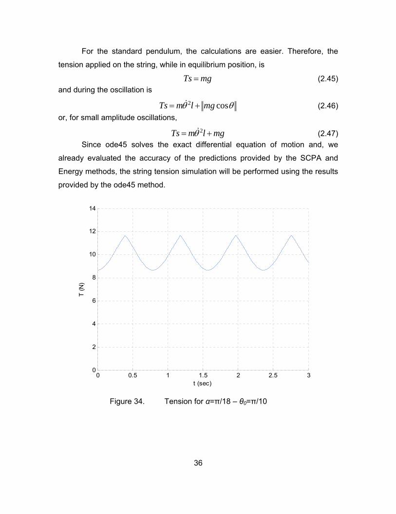
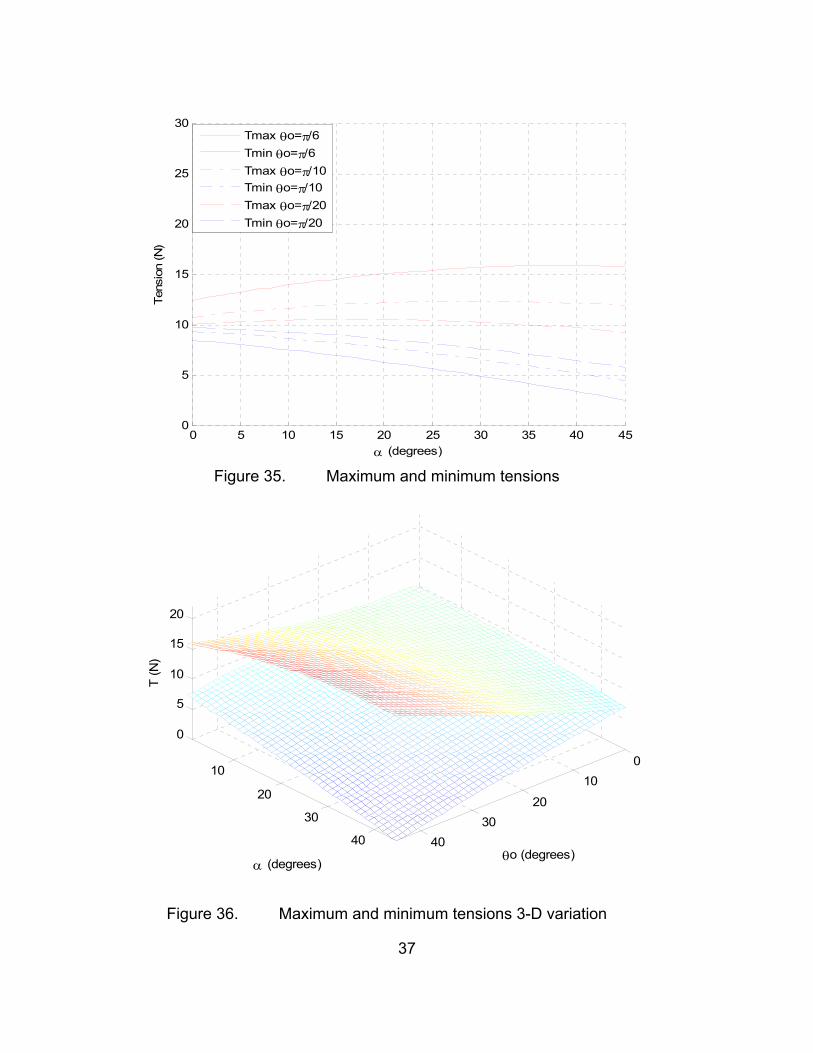
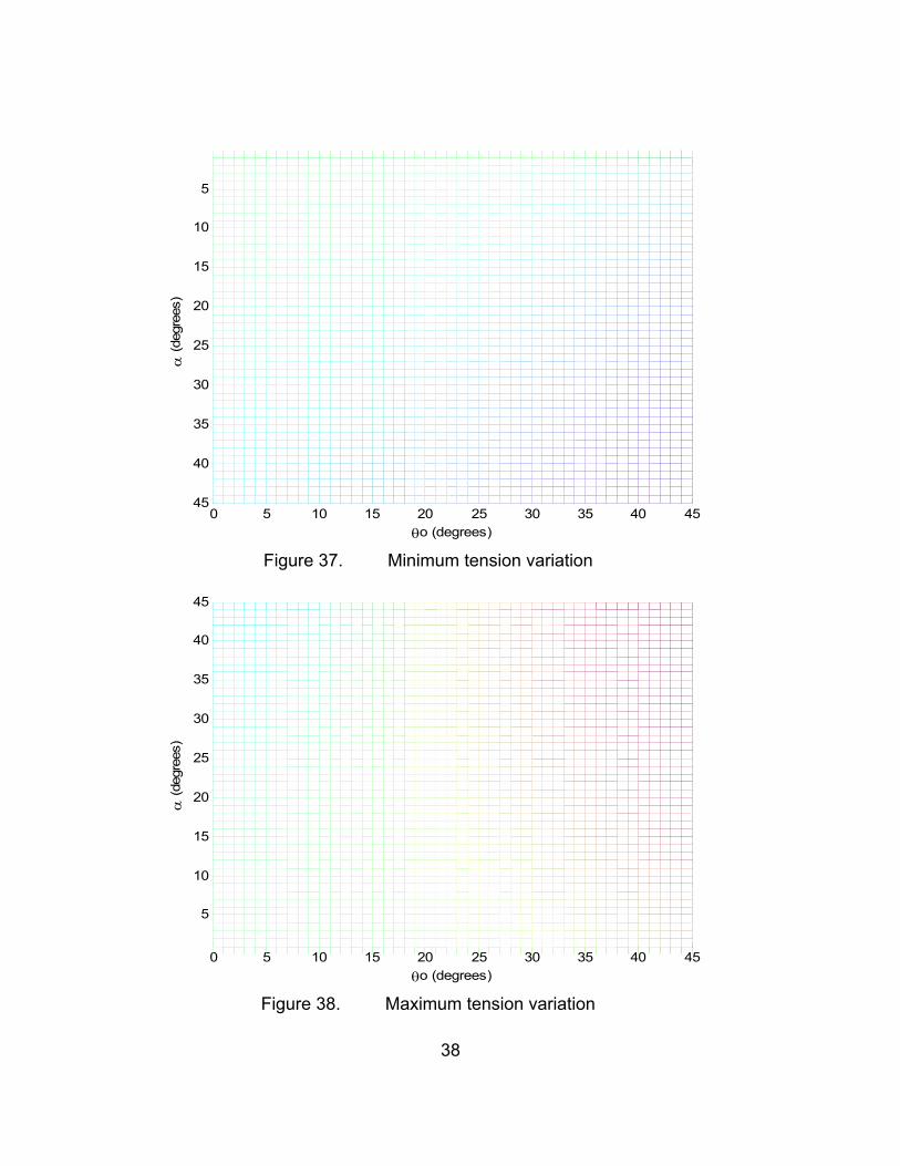
From Figures 35-38, we can evaluate the variation of maximum and
minimum tensions exerted on the strings with respect to both α and θο. On the
one hand, as expected, increasing θο increases the Tmax and decreases Tmin.
On the other hand, increasing α, and keeping θο constant, steadily decreases
Tmin. An interesting point is that Tmax does not exhibit the same behavior. In
Figure 39, we can see for which value of α we will have the maximum tension for
a range of initial displacements.
5 10 15 20 25 30 35 40 450
5
10
15
20
25
30
35
40
45
θo (degrees)
α (d
egre
es)
Figure 39. Characteristic angle producing the maximum tension for given θ0
40
C. NUMERICAL SIMULATION
A very precise method to simulate the response of the 2-pendulum is with
the use of the VISUAL NASTRAN 4-D software. In this section we attempt to
validate the methods that we used to predict the 2-pendulum response in
Chapter II, Section A, by comparing their results with those produced by VN 4-D.
1. VISUAL NASTRAN Software - SOLIDWORKS
To simulate the response of the 2-string pendulum in real time, a specific
procedure had to be followed. This procedure was initiated by designing a model
of a 2-string pendulum using SOLIDWORKS. This 3-D design software allows
the exact geometrical design of structural models, which are compatible with the
VN 4-D software. This model is then transferred into VN 4-D. The distinct
attribute of VN 4-D is to solve differential equations in 3-D space and time. The
final model used in VN 4-D was comprised of geometrical parts: mass properties
-- developed in SOLIDWORKS --, and their assembly -- developed partially in
SOLIDWORKS and partially in VN 4-D. The assembly constraints, which resulted
in the rigidity of the platform where the 2-pendulum support points were
positioned, were developed in SOLIDWORKS. The string constraints were
developed in VN 4-D. Before initiating each VN 4-D run, the mass had to be
positioned in the exact coordinates. This was the equivalent to a combination of
initial angular displacement θ0 and initial angular velocity θ0 of the VN 4-D. The
results of the simulations (in terms of mass position wrt which is the model’s
global system of axis, linear velocity, and tension of the strings) were then
exported into Microsoft Excel spreadsheets. In addition, as defined in Figures 5
and 6, the mass position results were processed to obtain the angular
displacement of the pendulum. Finally, all the above results were graphed with
the aid of Matlab. This allowed comparing them with our analysis results.
41
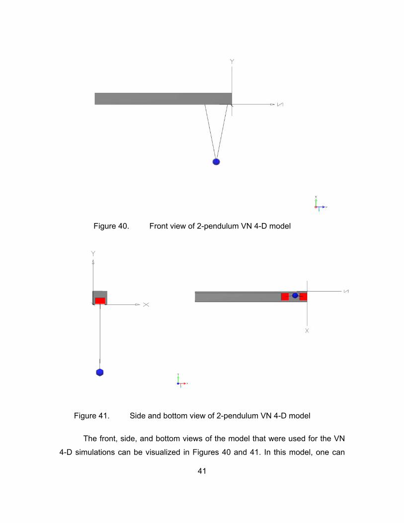
Figure 40. Front view of 2-pendulum VN 4-D model
Figure 41. Side and bottom view of 2-pendulum VN 4-D model
The front, side, and bottom views of the model that were used for the VN
4-D simulations can be visualized in Figures 40 and 41. In this model, one can
42
adjust the mass of the mass (blue sphere) and the characteristic angle by
altering the length of the strings (black lines) or the distance between the support
points (red cubes). In addition, an initial displacement can be applied to the mass
by precisely positioning the mass to a specific position in terms of an exact set of
coordinates (X,Y and Z), with respect to the Cartesian global system of axis
represented by the black arrows. It should be noted that the exact positioning of
the mass is not possible. For a few of the first time steps of the simulation, this
results in a slight deviation of the expected results. The numerical integration
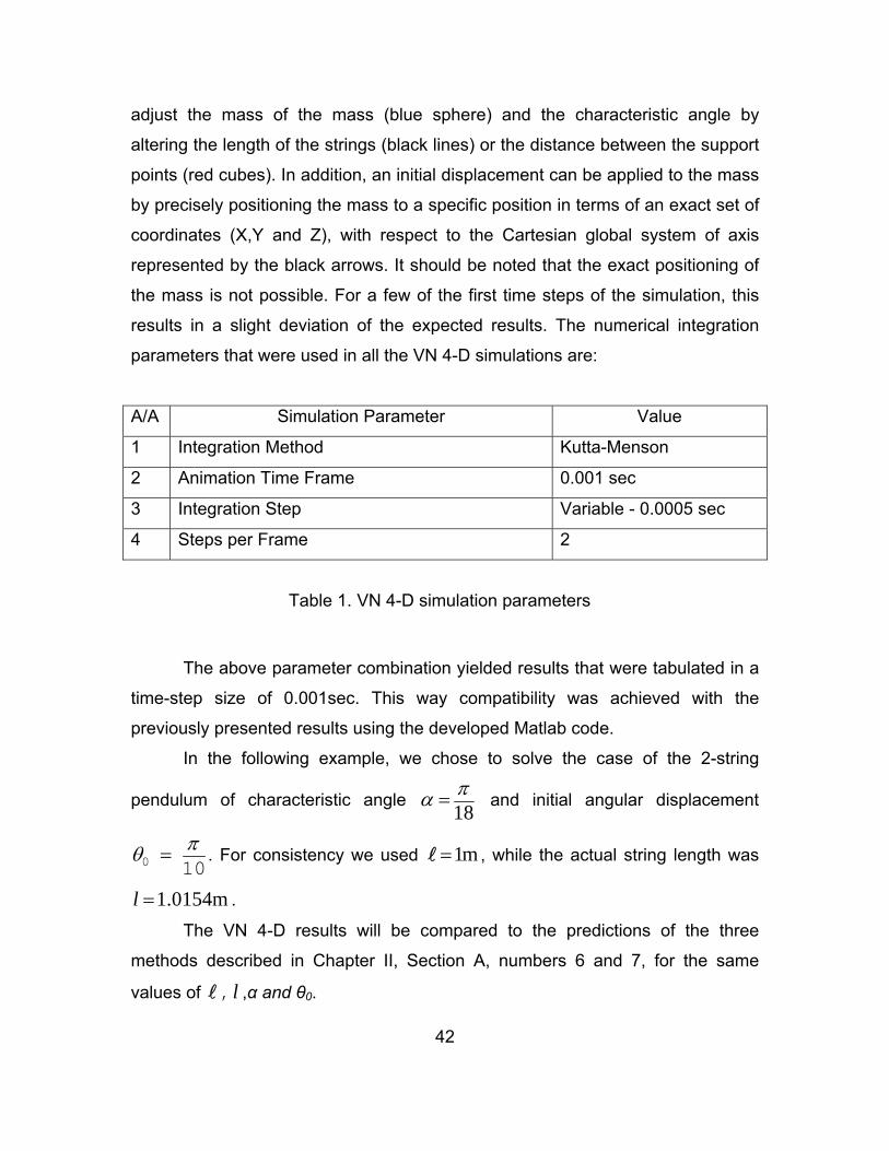
parameters that were used in all the VN 4-D simulations are:
A/A Simulation Parameter Value
1 Integration Method Kutta-Menson
2 Animation Time Frame 0.001 sec
3 Integration Step Variable - 0.0005 sec
4 Steps per Frame 2
Table 1. VN 4-D simulation parameters
The above parameter combination yielded results that were tabulated in a
time-step size of 0.001sec. This way compatibility was achieved with the
previously presented results using the developed Matlab code.
In the following example, we chose to solve the case of the 2-string
pendulum of characteristic angle 18πα = and initial angular displacement
πθ =0 10. For consistency we used 1m= , while the actual string length was
1.0154m=l .
The VN 4-D results will be compared to the predictions of the three
methods described in Chapter II, Section A, numbers 6 and 7, for the same
values of , l ,α and θ0.
43
0 1 2 3 4 5 6
-0.3
-0.2
-0.1
0
0.1
0.2
0.3
0.4
0.5
0.6
t (sec)
θ (ra
d)
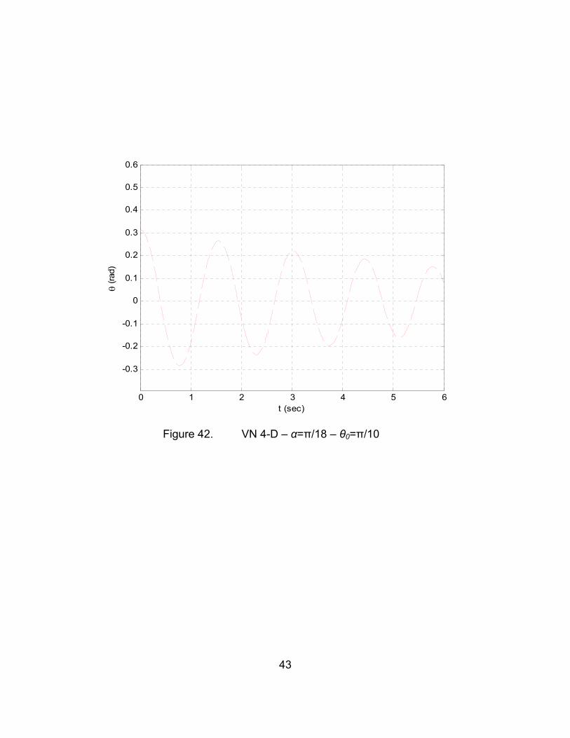
Figure 42. VN 4-D – α=π/18 – θ0=π/10
44
0 1 2 3 4 5 6
-0.3
-0.2
-0.1
0
0.1
0.2
0.3
0.4
0.5
0.6
t (sec)
θ (ra
d)ODE45SCPA methodEnergy method
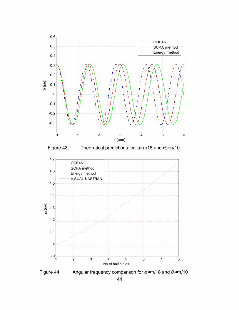
Figure 43. Theoretical predictions for α=π/18 and θ0=π/10
1 2 3 4 5 6 7 83.9
4
4.1
4.2
4.3
4.4
4.5
4.6
4.7
No of half cicles
ω (r
ad)
ODE45SCPA methodEnergy methodVISUAL NASTRAN
Figure 44. Angular frequency comparison for α =π/18 and θ0=π/10
45
0 1 2 3 4 5 6-1.5
-1
-0.5
0
0.5
1
1.5
t (sec)
θ' (r
ad/s
ec)
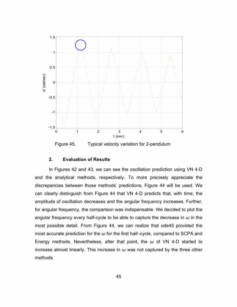
Figure 45. Typical velocity variation for 2-pendulum
2. Evaluation of Results
In Figures 42 and 43, we can see the oscillation prediction using VN 4-D
and the analytical methods, respectively. To more precisely appreciate the
discrepancies between those methods’ predictions, Figure 44 will be used. We
can clearly distinguish from Figure 44 that VN 4-D predicts that, with time, the
amplitude of oscillation decreases and the angular frequency increases. Further,
for angular frequency, the comparison was indispensable. We decided to plot the
angular frequency every half-cycle to be able to capture the decrease in ω in the
most possible detail. From Figure 44, we can realize that ode45 provided the
most accurate prediction for the ω for the first half–cycle, compared to SCPA and
Energy methods. Nevertheless, after that point, the ω of VN 4-D started to
increase almost linearly. This increase in ω was not captured by the three other
methods.
46
To understand why this increase in ω takes place, we plotted the angular
frequency of oscillation predicted by VN 4-D. As seen in Figure 45, for every half-
cycle when the mass reached the point where it switched strings about which it
oscillated, the velocity magnitude dropped by a certain amount. This
discontinuity, just before and after the switch point in velocity magnitude, raises
questions about energy conservation. In the following sections, we are going to
investigate in more details the dynamics that surface at this point and their effect
in terms of energy loss of the oscillation mass.
D. THE REAL 2-PENDULUM
1. Velocity and Force Vector Analysis-Impact Dynamics
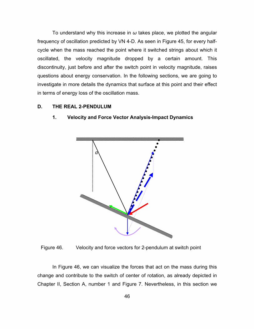
Figure 46. Velocity and force vectors for 2-pendulum at switch point
In Figure 46, we can visualize the forces that act on the mass during this
change and contribute to the switch of center of rotation, as already depicted in
Chapter II, Section A, number 1 and Figure 7. Nevertheless, in this section we
α
47
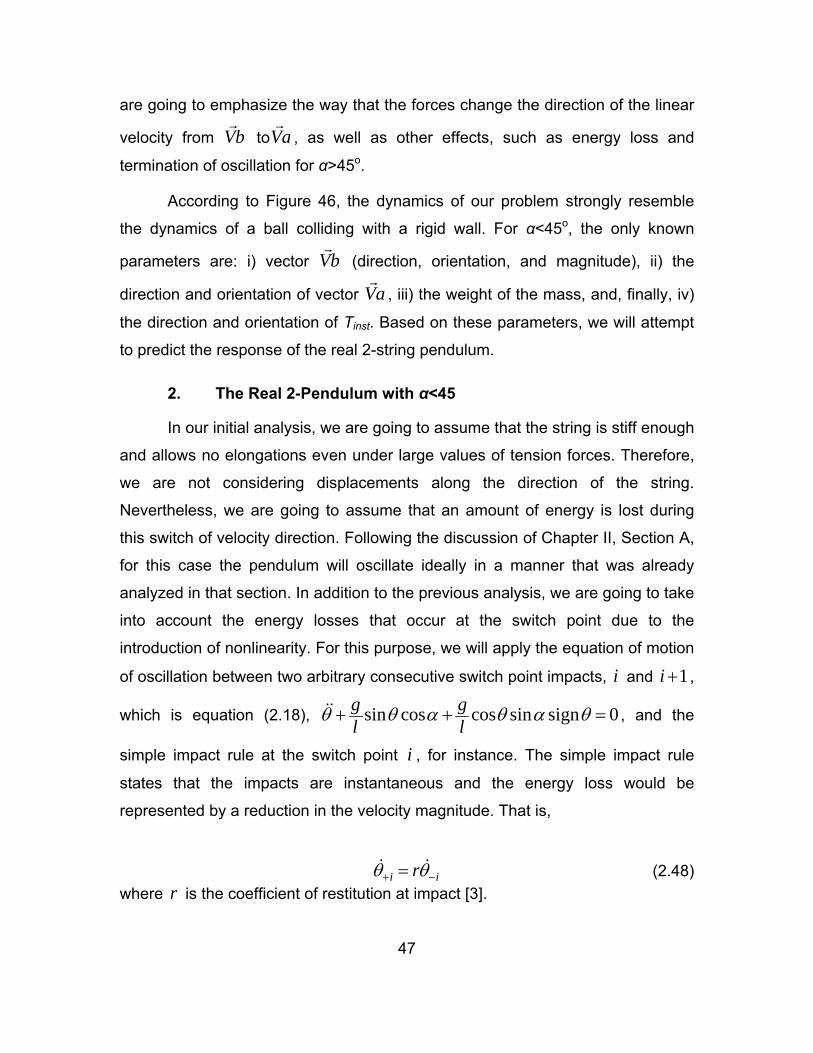
are going to emphasize the way that the forces change the direction of the linear
velocity from Vb toVa , as well as other effects, such as energy loss and
termination of oscillation for α>45o.
According to Figure 46, the dynamics of our problem strongly resemble
the dynamics of a ball colliding with a rigid wall. For α<45o, the only known
parameters are: i) vector Vb (direction, orientation, and magnitude), ii) the
direction and orientation of vector Va , iii) the weight of the mass, and, finally, iv)
the direction and orientation of Tinst. Based on these parameters, we will attempt
to predict the response of the real 2-string pendulum.
2. The Real 2-Pendulum with α<45
In our initial analysis, we are going to assume that the string is stiff enough
and allows no elongations even under large values of tension forces. Therefore,
we are not considering displacements along the direction of the string.
Nevertheless, we are going to assume that an amount of energy is lost during
this switch of velocity direction. Following the discussion of Chapter II, Section A,
for this case the pendulum will oscillate ideally in a manner that was already
analyzed in that section. In addition to the previous analysis, we are going to take
into account the energy losses that occur at the switch point due to the
introduction of nonlinearity. For this purpose, we will apply the equation of motion
of oscillation between two arbitrary consecutive switch point impacts, i and 1+i ,
which is equation (2.18), sin cos cos sin sign 0θ θ α θ α θ+ + =g gl l
, and the
simple impact rule at the switch point i , for instance. The simple impact rule
states that the impacts are instantaneous and the energy loss would be
represented by a reduction in the velocity magnitude. That is,
θ θ+ −=i ir (2.48) where r is the coefficient of restitution at impact [3].
48
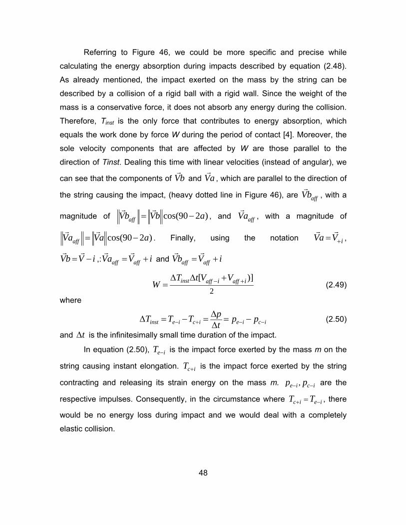
Referring to Figure 46, we could be more specific and precise while
calculating the energy absorption during impacts described by equation (2.48).
As already mentioned, the impact exerted on the mass by the string can be
described by a collision of a rigid ball with a rigid wall. Since the weight of the
mass is a conservative force, it does not absorb any energy during the collision.
Therefore, Tinst is the only force that contributes to energy absorption, which
equals the work done by force W during the period of contact [4]. Moreover, the
sole velocity components that are affected by W are those parallel to the
direction of Tinst. Dealing this time with linear velocities (instead of angular), we
can see that the components of Vb and Va , which are parallel to the direction of
the string causing the impact, (heavy dotted line in Figure 46), are affVb , with a
magnitude of cos(90 2 )= −affVb Vb a , and affVa , with a magnitude of
cos(90 2 )= −affVa Va a . Finally, using the notation += iVa V ,
= −Vb V i ,: = +aff affVa V i and = +aff affVb V i
2
[ )]− +∆ ∆ += inst aff affi iT t V V
W (2.49)
where
− + − −∆∆ = − = = −∆inst e i c i e i c ipT T T p pt
(2.50)
and ∆t is the infinitesimally small time duration of the impact.
In equation (2.50), −e iT is the impact force exerted by the mass m on the
string causing instant elongation. +c iT is the impact force exerted by the string
contracting and releasing its strain energy on the mass m. ,− −e i c ip p are the
respective impulses. Consequently, in the circumstance where + −=c i e iT T , there
would be no energy loss during impact and we would deal with a completely
elastic collision.
49
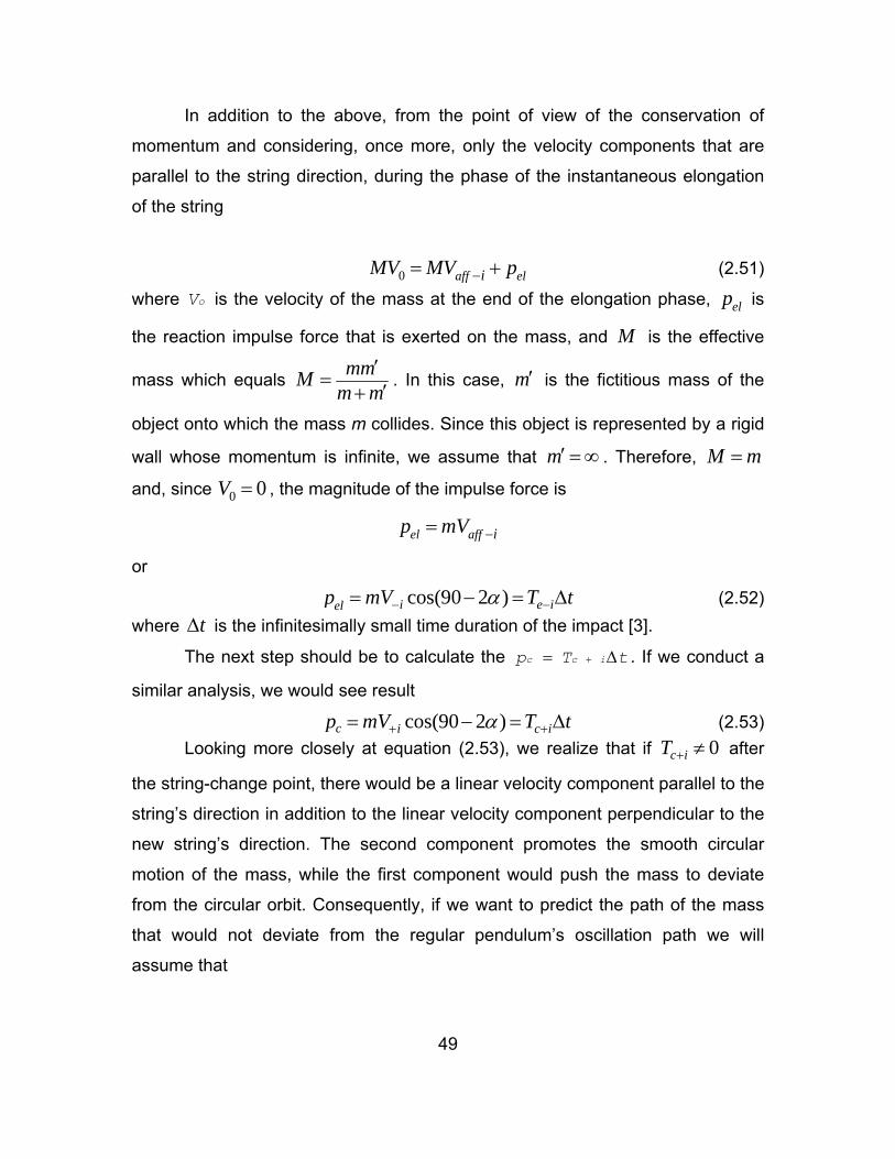
In addition to the above, from the point of view of the conservation of
momentum and considering, once more, only the velocity components that are
parallel to the string direction, during the phase of the instantaneous elongation
of the string
0 −= +aff eliMV MV p (2.51)
where oV is the velocity of the mass at the end of the elongation phase, elp is
the reaction impulse force that is exerted on the mass, and M is the effective
mass which equals ′=′+
mmMm m
. In this case, ′m is the fictitious mass of the
object onto which the mass m collides. Since this object is represented by a rigid
wall whose momentum is infinite, we assume that ′ = ∞m . Therefore, =M m
and, since 0 0=V , the magnitude of the impulse force is
−=el aff ip mV
or
cos(90 2 )α− −= − = ∆i e ielp mV T t (2.52) where ∆t is the infinitesimally small time duration of the impact [3].
The next step should be to calculate the c c ip T t+= ∆ . If we conduct a
similar analysis, we would see result
cos(90 2 )α+ += − = ∆c i c ip mV T t (2.53) Looking more closely at equation (2.53), we realize that if 0+ ≠c iT after
the string-change point, there would be a linear velocity component parallel to the
string’s direction in addition to the linear velocity component perpendicular to the
new string’s direction. The second component promotes the smooth circular
motion of the mass, while the first component would push the mass to deviate
from the circular orbit. Consequently, if we want to predict the path of the mass
that would not deviate from the regular pendulum’s oscillation path we will
assume that
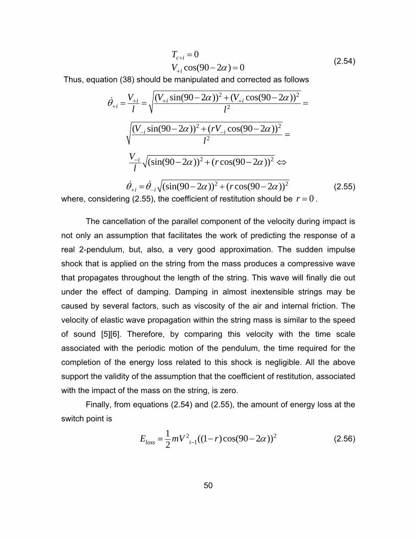
50
0
cos(90 2 ) 0α+
+
=− =
c i
i
TV
(2.54)
Thus, equation (38) should be manipulated and corrected as follows
2 2
2( sin(90 2 )) ( cos(90 2 ))α αθ + + +
+− + −= = =i i i
iV V Vl l
2 2
2( sin(90 2 )) ( cos(90 2 ))α α− −− + − =i iV rV
l
2 2(sin(90 2 )) ( cos(90 2 ))α α− − + − ⇔iV rl
2 2(sin(90 2 )) ( cos(90 2 ))θ θ α α+ −= − + −i i r (2.55) where, considering (2.55), the coefficient of restitution should be 0=r .
The cancellation of the parallel component of the velocity during impact is
not only an assumption that facilitates the work of predicting the response of a
real 2-pendulum, but, also, a very good approximation. The sudden impulse
shock that is applied on the string from the mass produces a compressive wave
that propagates throughout the length of the string. This wave will finally die out
under the effect of damping. Damping in almost inextensible strings may be
caused by several factors, such as viscosity of the air and internal friction. The
velocity of elastic wave propagation within the string mass is similar to the speed
of sound [5][6]. Therefore, by comparing this velocity with the time scale
associated with the periodic motion of the pendulum, the time required for the
completion of the energy loss related to this shock is negligible. All the above
support the validity of the assumption that the coefficient of restitution, associated
with the impact of the mass on the string, is zero.
Finally, from equations (2.54) and (2.55), the amount of energy loss at the
switch point is
2 21
1 ((1 )cos(90 2 ))2
α−= − −ilossE mV r (2.56)
51
The system of equations (2.18) and (2.48) or (2.55) can be solved
numerically using a constant time step of 0.001sec∆ =t and the forward
difference scheme. This takes into account equation (2.48) or (2.55). The Matlab
code, Program_3.m, provides the solution to the system of equations for
predetermined number of periods.
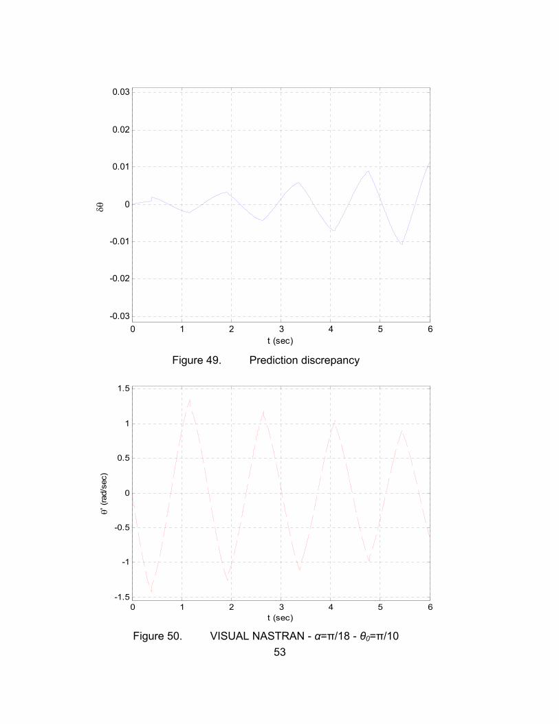
In the following sections, we are going to compare the prediction of the 2-
pendulum response in terms of angular displacement, angular velocity, and string
tension. We will use the above m-file (solving equations (2.18) and (2.55))
combined with those obtained from VISUAL NASTRAN. Additionally, we will plot
the phase diagrams for each method, as well as the discrepancy between the
prediction and the VISUAL NASTRAN simulation results. This will better validate
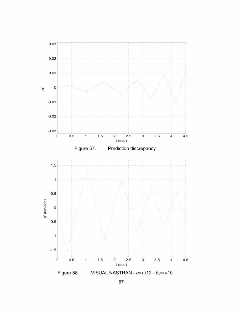
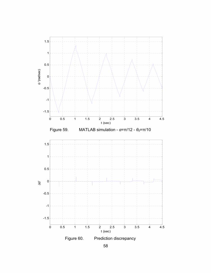
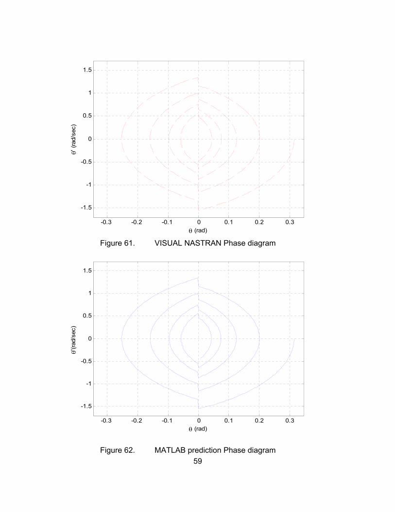
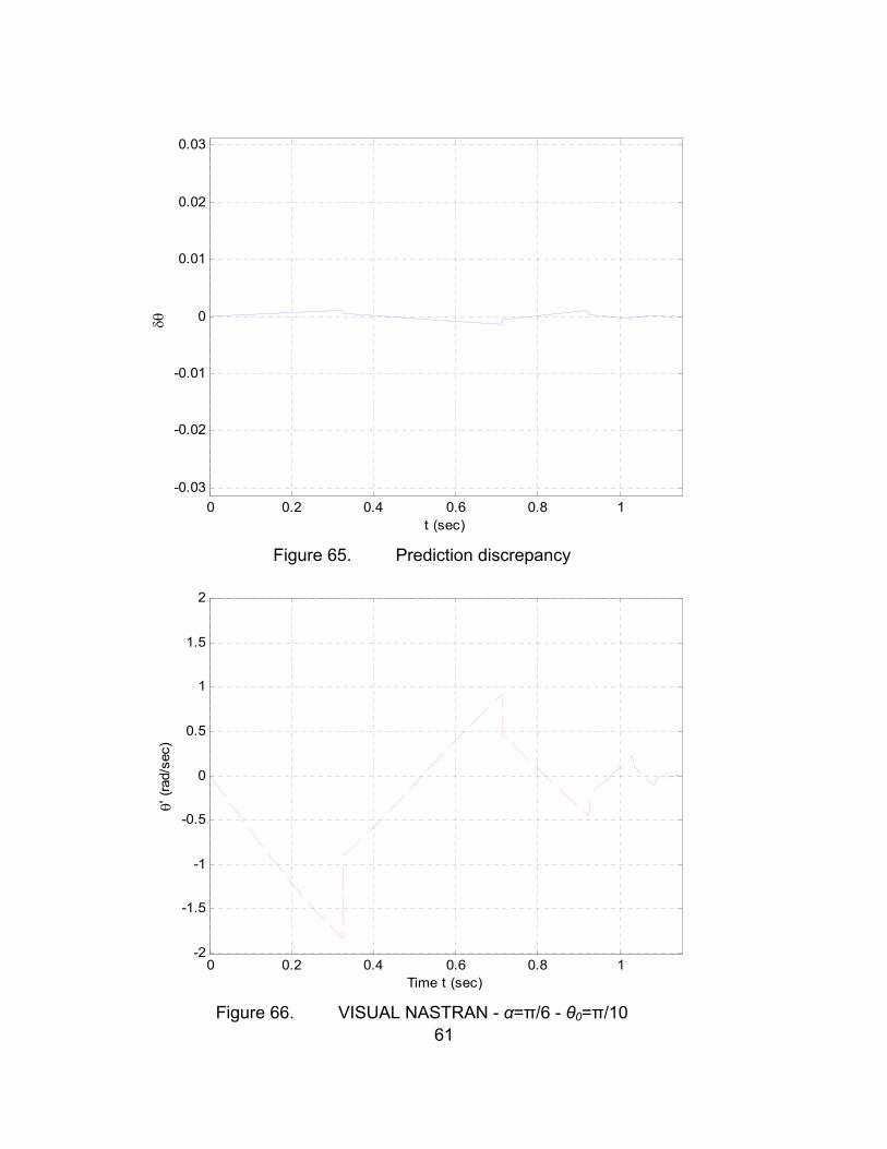
the precision of the Matlab code.
52
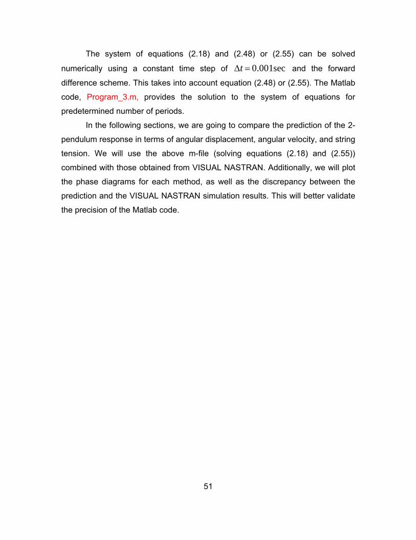
a. Angular Displacement and Velocity Comparison
0 1 2 3 4 5 6
-0.3
-0.2
-0.1
0
0.1
0.2
0.3
t (sec)
θ (ra
d)
Figure 47. VISUAL NASTRAN - α=π/18 – θ0=π/10
0 1 2 3 4 5 6
-0.3
-0.2
-0.1
0
0.1
0.2
0.3
t (sec)
θ (ra
d)
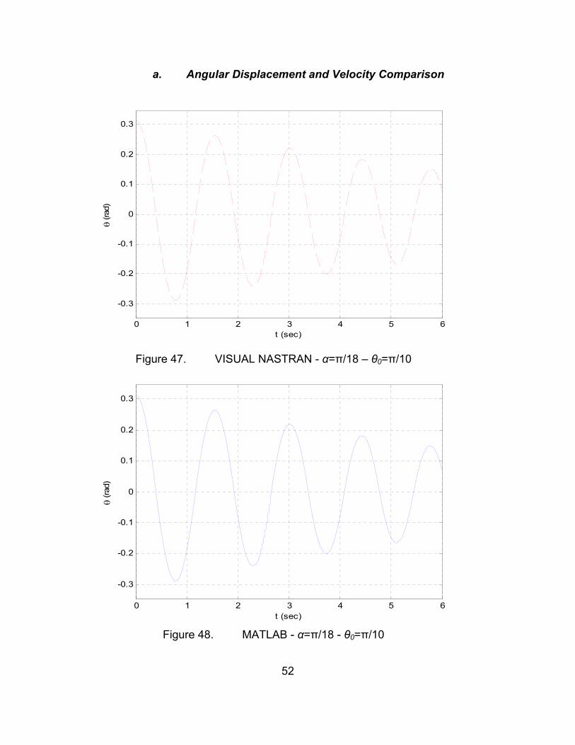
Figure 48. MATLAB - α=π/18 - θ0=π/10
53
0 1 2 3 4 5 6-0.03
-0.02
-0.01
0
0.01
0.02
0.03
t (sec)
δθ
Figure 49. Prediction discrepancy
0 1 2 3 4 5 6-1.5
-1
-0.5
0
0.5
1
1.5
t (sec)
θ' (r
ad/s
ec)
Figure 50. VISUAL NASTRAN - α=π/18 - θ0=π/10
54
0 1 2 3 4 5 6-1.5
-1
-0.5
0
0.5
1
1.5
t (sec)
θ '(r
ad/s
ec)
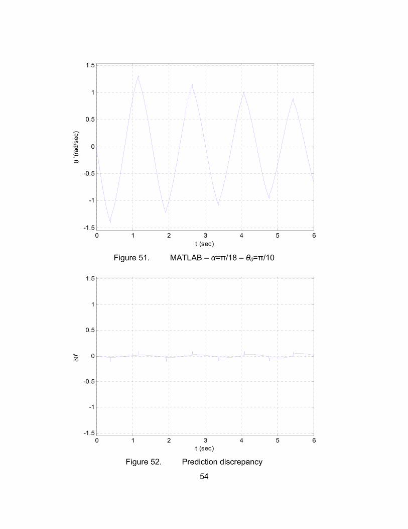
Figure 51. MATLAB – α=π/18 – θ0=π/10
0 1 2 3 4 5 6-1.5
-1
-0.5
0
0.5
1
1.5
t (sec)
δθ'
Figure 52. Prediction discrepancy
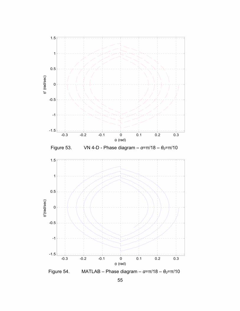
55
-0.3 -0.2 -0.1 0 0.1 0.2 0.3-1.5
-1
-0.5
0
0.5
1
1.5
θ (rad)
θ' (r
ad/s
ec)
Figure 53. VN 4-D - Phase diagram – α=π/18 – θ0=π/10
-0.3 -0.2 -0.1 0 0.1 0.2 0.3-1.5
-1
-0.5
0
0.5
1
1.5
θ (rad)
θ'(ra
d/se
c)
Figure 54. MATLAB – Phase diagram – α=π/18 – θ0=π/10
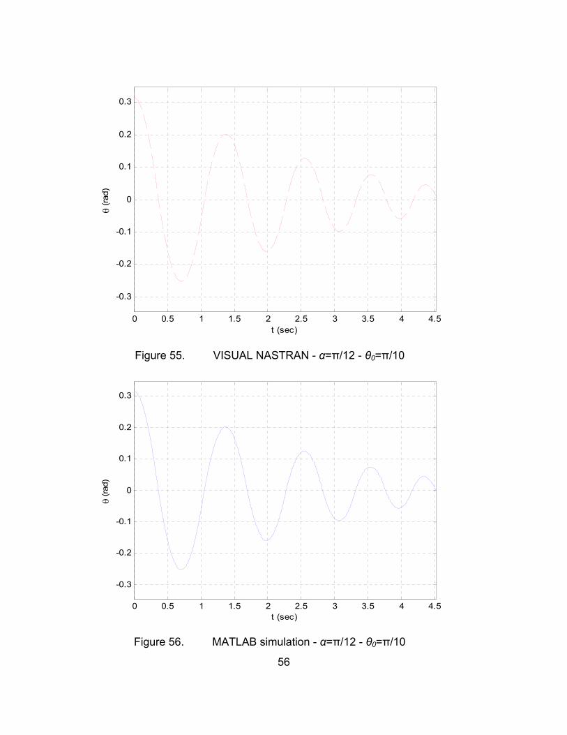
56
0 0.5 1 1.5 2 2.5 3 3.5 4 4.5
-0.3
-0.2
-0.1
0
0.1
0.2
0.3
t (sec)
θ (ra
d)
Figure 55. VISUAL NASTRAN - α=π/12 - θ0=π/10
0 0.5 1 1.5 2 2.5 3 3.5 4 4.5
-0.3
-0.2
-0.1
0
0.1
0.2
0.3
t (sec)
θ (ra
d)
Figure 56. MATLAB simulation - α=π/12 - θ0=π/10
57
0 0.5 1 1.5 2 2.5 3 3.5 4 4.5-0.03
-0.02
-0.01
0
0.01
0.02
0.03
t (sec)
δθ
Figure 57. Prediction discrepancy
0 0.5 1 1.5 2 2.5 3 3.5 4 4.5
-1.5
-1
-0.5
0
0.5
1
1.5
t (sec)
θ' (r
ad/s
ec)
Figure 58. VISUAL NASTRAN - α=π/12 - θ0=π/10
58
0 0.5 1 1.5 2 2.5 3 3.5 4 4.5
-1.5
-1
-0.5
0
0.5
1
1.5
t (sec)
θ '(r
ad/s
ec)
Figure 59. MATLAB simulation - α=π/12 - θ0=π/10
0 0.5 1 1.5 2 2.5 3 3.5 4 4.5
-1.5
-1
-0.5
0
0.5
1
1.5
t (sec)
δθ'
Figure 60. Prediction discrepancy
59
-0.3 -0.2 -0.1 0 0.1 0.2 0.3
-1.5
-1
-0.5
0
0.5
1
1.5
θ (rad)
θ' (r
ad/s
ec)
Figure 61. VISUAL NASTRAN Phase diagram
-0.3 -0.2 -0.1 0 0.1 0.2 0.3
-1.5
-1
-0.5
0
0.5
1
1.5
θ (rad)
θ'(ra
d/se
c)
Figure 62. MATLAB prediction Phase diagram

60
0 0.2 0.4 0.6 0.8 1
-0.3
-0.2
-0.1
0
0.1
0.2
0.3
t (sec)
θ (ra
d)
Figure 63. VISUAL NASTRAN - α=π/6 - θ0=π/10
0 0.2 0.4 0.6 0.8 1
-0.3
-0.2
-0.1
0
0.1
0.2
0.3
t (sec)
θ (ra
d)
Figure 64. MATLAB simulation – α=π/6 - θ0=π/10
61
0 0.2 0.4 0.6 0.8 1-0.03
-0.02
-0.01
0
0.01
0.02
0.03
t (sec)
δθ
Figure 65. Prediction discrepancy
0 0.2 0.4 0.6 0.8 1-2
-1.5
-1
-0.5
0
0.5
1
1.5
2
Time t (sec)
θ' (r
ad/s
ec)
Figure 66. VISUAL NASTRAN - α=π/6 - θ0=π/10
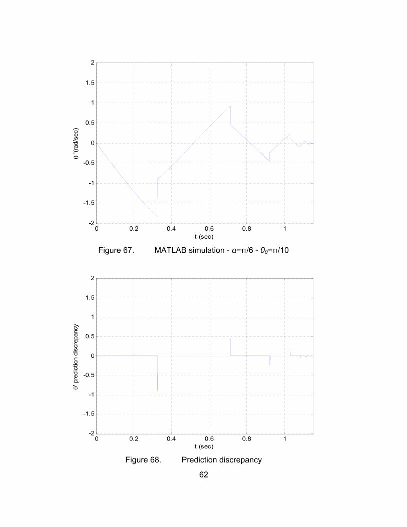
62
0 0.2 0.4 0.6 0.8 1-2
-1.5
-1
-0.5
0
0.5
1
1.5
2
t (sec)
θ '(r
ad/s
ec)
Figure 67. MATLAB simulation - α=π/6 - θ0=π/10
0 0.2 0.4 0.6 0.8 1-2
-1.5
-1
-0.5
0
0.5
1
1.5
2
t (sec)
θ' p
redi
ctio
n di
scre
panc
y
Figure 68. Prediction discrepancy
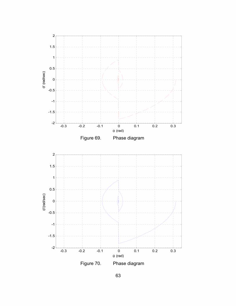
63
-0.3 -0.2 -0.1 0 0.1 0.2 0.3-2
-1.5
-1
-0.5
0
0.5
1
1.5
2
θ (rad)
θ' (r
ad/s
ec)
Figure 69. Phase diagram
-0.3 -0.2 -0.1 0 0.1 0.2 0.3-2
-1.5
-1
-0.5
0
0.5
1
1.5
2
θ (rad)
θ'(ra
d/se
c)
Figure 70. Phase diagram
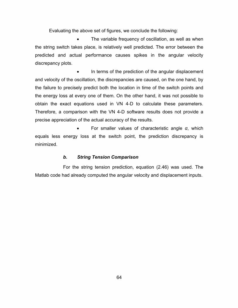
64
Evaluating the above set of figures, we conclude the following:
• The variable frequency of oscillation, as well as when
the string switch takes place, is relatively well predicted. The error between the
predicted and actual performance causes spikes in the angular velocity
discrepancy plots.
• In terms of the prediction of the angular displacement
and velocity of the oscillation, the discrepancies are caused, on the one hand, by
the failure to precisely predict both the location in time of the switch points and
the energy loss at every one of them. On the other hand, it was not possible to
obtain the exact equations used in VN 4-D to calculate these parameters.
Therefore, a comparison with the VN 4-D software results does not provide a
precise appreciation of the actual accuracy of the results.
• For smaller values of characteristic angle α, which
equals less energy loss at the switch point, the prediction discrepancy is
minimized.
b. String Tension Comparison
For the string tension prediction, equation (2.46) was used. The
Matlab code had already computed the angular velocity and displacement inputs.
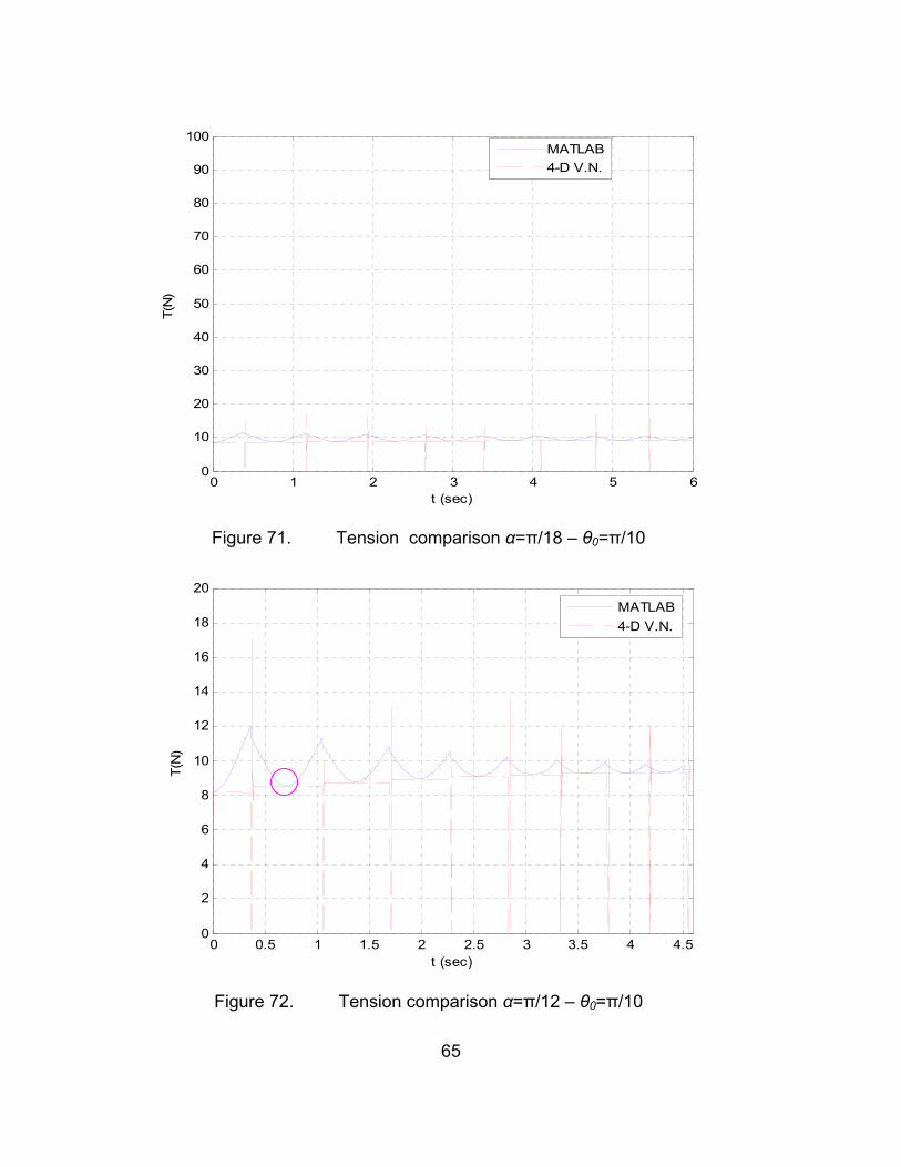
65
0 1 2 3 4 5 60
10
20
30
40
50
60
70
80
90
100
t (sec)
T(N
)
MATLAB4-D V.N.
Figure 71. Tension comparison α=π/18 – θ0=π/10
0 0.5 1 1.5 2 2.5 3 3.5 4 4.50
2
4
6
8
10
12
14
16
18
20
t (sec)
T(N
)
MATLAB4-D V.N.
Figure 72. Tension comparison α=π/12 – θ0=π/10
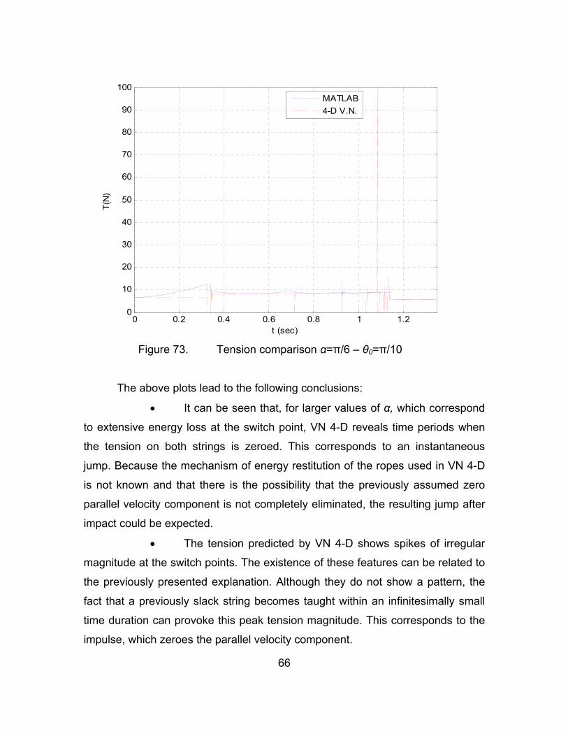
66
0 0.2 0.4 0.6 0.8 1 1.20
10
20
30
40
50
60
70
80
90
100
t (sec)
T(N
) MATLAB4-D V.N.
Figure 73. Tension comparison α=π/6 – θ0=π/10
The above plots lead to the following conclusions:
• It can be seen that, for larger values of α, which correspond
to extensive energy loss at the switch point, VN 4-D reveals time periods when
the tension on both strings is zeroed. This corresponds to an instantaneous
jump. Because the mechanism of energy restitution of the ropes used in VN 4-D
is not known and that there is the possibility that the previously assumed zero
parallel velocity component is not completely eliminated, the resulting jump after
impact could be expected.
• The tension predicted by VN 4-D shows spikes of irregular
magnitude at the switch points. The existence of these features can be related to
the previously presented explanation. Although they do not show a pattern, the
fact that a previously slack string becomes taught within an infinitesimally small
time duration can provoke this peak tension magnitude. This corresponds to the
impulse, which zeroes the parallel velocity component.
67
• The Matlab code tension prediction coincides with the VN 4-
D only at the instances when the mass velocity is zero (indicated with a purple
circle in Figure 72). Therefore, the VN 4-D tension prediction is not in accordance
with equation (2.46). To understand this unexpected result, a model of two
standard pendula -- one with a string and the other with a massless rod -- was
used to calculate the tension during free oscillation with an arbitrary initial
displacement. The results revealed that the standard rod pendulum’s tension
agrees with equation (2.46), while the standard string pendulum’s tension does
not. Moreover, an effort was made to understand the pattern that provided the
string tension results. After some trial and error efforts, the equation that provided
an almost identical tension prediction was
2
cos2θ θ−= +m lT mg (2.57)
Efforts were made to understand the above equation, but, unfortunately,
the MSC Software no longer supported the specific software. Consequently,
further tension comparisons with VN 4-D will not be performed and, also, the
Matlab results will be presented without validation from the VN 4-D results.
3. The Real 2-Pendulum with a≥45
In the case that α=45o, when applying equation (2.55), we realize that for
0r = all the kinetic energy of the pendulum would be absorbed by the string
during impact. Thus, the oscillation would be terminated. The above can be
visualized from the following graphs, where VISUAL NASTRAN and MATLAB
simulations are used to provide the response of the 2-string pendulum with
α=45o.
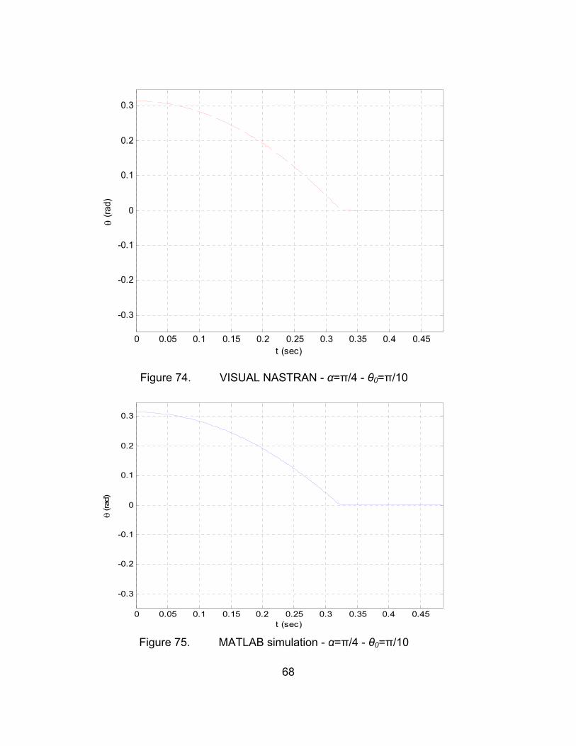
68
0 0.05 0.1 0.15 0.2 0.25 0.3 0.35 0.4 0.45
-0.3
-0.2
-0.1
0
0.1
0.2
0.3
t (sec)
θ (ra
d)
Figure 74. VISUAL NASTRAN - α=π/4 - θ0=π/10
0 0.05 0.1 0.15 0.2 0.25 0.3 0.35 0.4 0.45
-0.3
-0.2
-0.1
0
0.1
0.2
0.3
t (sec)
θ (ra
d)
Figure 75. MATLAB simulation - α=π/4 - θ0=π/10
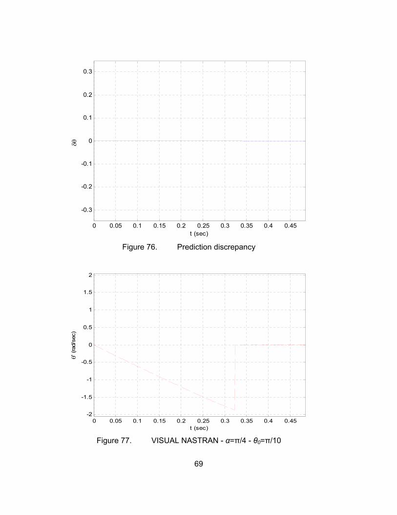
69
0 0.05 0.1 0.15 0.2 0.25 0.3 0.35 0.4 0.45
-0.3
-0.2
-0.1
0
0.1
0.2
0.3
t (sec)
δθ
Figure 76. Prediction discrepancy
0 0.05 0.1 0.15 0.2 0.25 0.3 0.35 0.4 0.45-2
-1.5
-1
-0.5
0
0.5
1
1.5
2
t (sec)
θ' (r
ad/s
ec)
Figure 77. VISUAL NASTRAN - α=π/4 - θ0=π/10
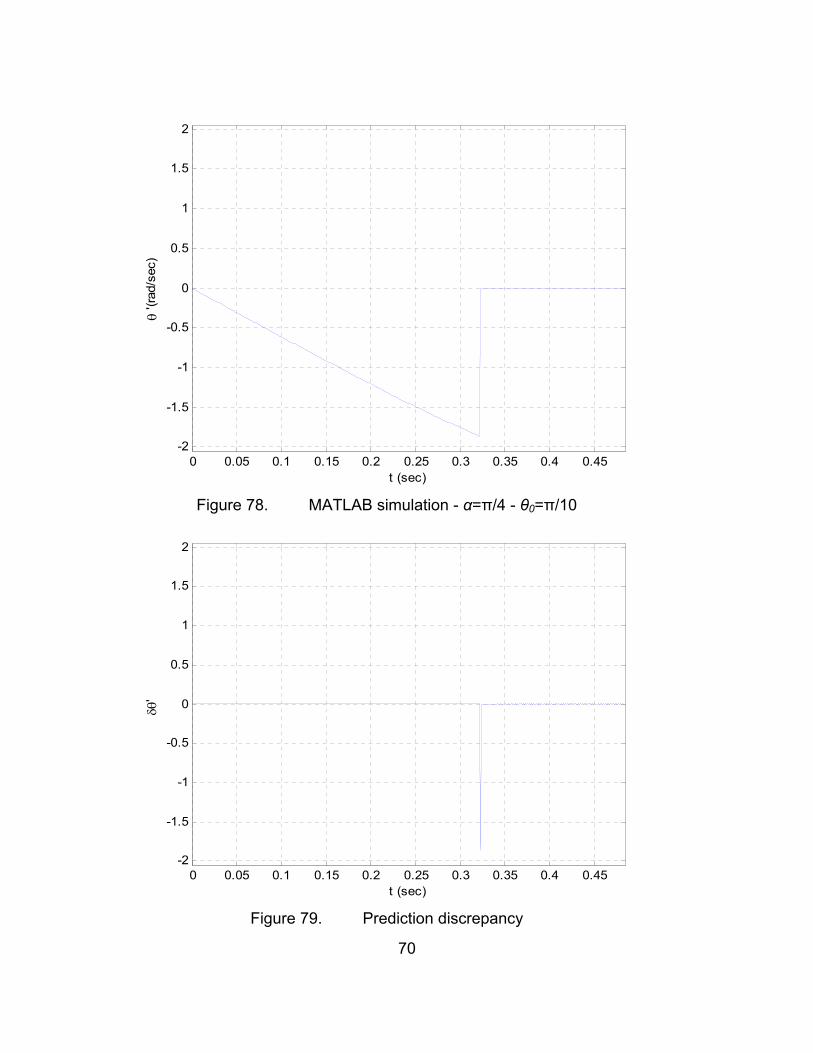
70
0 0.05 0.1 0.15 0.2 0.25 0.3 0.35 0.4 0.45-2
-1.5
-1
-0.5
0
0.5
1
1.5
2
t (sec)
θ '(r
ad/s
ec)
Figure 78. MATLAB simulation - α=π/4 - θ0=π/10
0 0.05 0.1 0.15 0.2 0.25 0.3 0.35 0.4 0.45-2
-1.5
-1
-0.5
0
0.5
1
1.5
2
t (sec)
δθ'
Figure 79. Prediction discrepancy
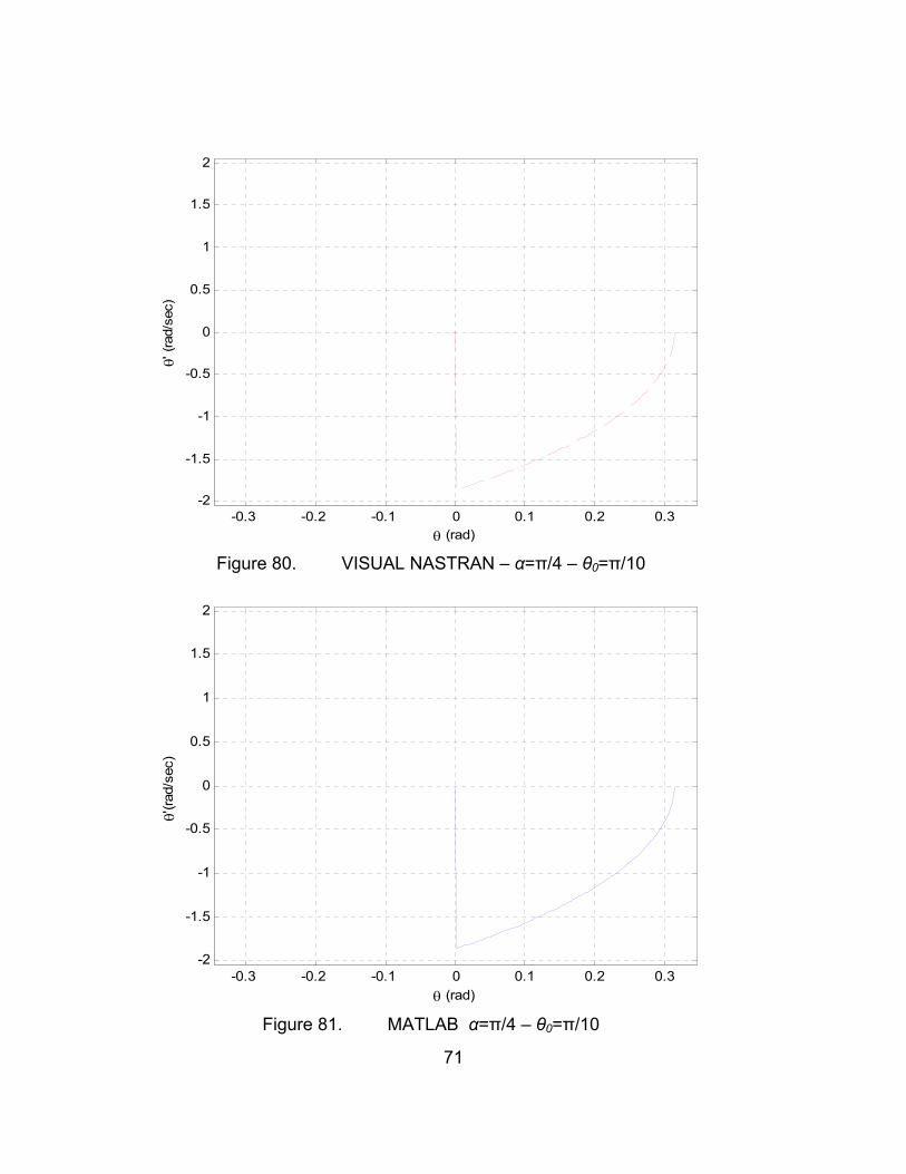
71
-0.3 -0.2 -0.1 0 0.1 0.2 0.3-2
-1.5
-1
-0.5
0
0.5
1
1.5
2
θ (rad)
θ' (r
ad/s
ec)
Figure 80. VISUAL NASTRAN – α=π/4 – θ0=π/10
-0.3 -0.2 -0.1 0 0.1 0.2 0.3-2
-1.5
-1
-0.5
0
0.5
1
1.5
2
θ (rad)
θ'(ra
d/se
c)
Figure 81. MATLAB α=π/4 – θ0=π/10
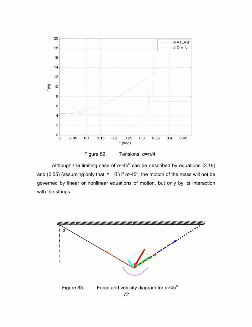
72
0 0.05 0.1 0.15 0.2 0.25 0.3 0.35 0.4 0.450
2
4
6
8
10
12
14
16
18
20
t (sec)
T(N
)
MATLAB4-D V.N.
Figure 82. Tensions α=π/4
Although the limiting case of α=45o can be described by equations (2.18)
and (2.55) (assuming only that 0r = ) if α>45o, the motion of the mass will not be
governed by linear or nonlinear equations of motion, but only by its interaction
with the strings.
Figure 83. Force and velocity diagram for α>45o
α

73
According to Figure 83, the linear velocity before the switch point Vb (red
vector) is composed of two components, 1Vb and 2Vb (turquoise and green
vectors, respectively). At the instance when the right string becomes tight, the
tension of the string (blue vector) exerts an impulse affecting 2Vb . Irrespective to
the value of the restitution coefficient that governs this impact, 1Vb cannot
promote the circular motion of the mass with respect to the right string due to its
direction. Contrarily, the left string, which becomes slack after the switch point for
α<45o, continues to be tight and exerts, along with the right string, an impulse on
the mass opposing 1Vb (orange vectors). Thus, either the mass will bounce or it
will come to rest. This depends on the restitution coefficient. Consequently, if we
preserve the assumption that 0r = for all mass-string impact interactions, after
the mass reaches the switch point, it comes to rest.
E. THE DRIVEN PENDULUM
Extending the analysis performed in the previous sections, we should
include the case of the pendulum in which the supporting point, or points,
undergoes motion due to forcing. The moving support induces complexity to the
response of the pendulum that may not end in oscillatory behavior [6].
1. The Standard Driven Pendulum
Consider a standard pendulum which, at an arbitrary moment of the
oscillation, has an angular displacement θ, where 2 2π πθ− ≤ ≤ . We define a
world system of axis where x-axis points to the right and y-axis points upwards.
An arbitrary motion drives the support point of the pendulum, whose acceleration
at that moment has both a horizontal and a vertical component.
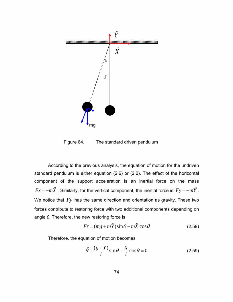
74
Figure 84. The standard driven pendulum
According to the previous analysis, the equation of motion for the undriven
standard pendulum is either equation (2.6) or (2.2). The effect of the horizontal
component of the support acceleration is an inertial force on the mass
Fx mX= − . Similarly, for the vertical component, the inertial force is Fy mY= − .
We notice that Fy has the same direction and orientation as gravity. These two
forces contribute to restoring force with two additional components depending on
angle θ. Therefore, the new restoring force is
( )sin cosθ θ= + −Fr mg mY mX (2.58)
Therefore, the equation of motion becomes
( ) sin cos 0θ θ θ++ − =g Y Xl l
(2.59)
θ
X
Y
mg
75
Finally, from equation (2.59) we can draw the conclusion that, due to the
horizontal acceleration, the pendulum will initiate oscillations even without the
existence of initial displacement or initial velocity. Thus, for θ=θ0=0, equation,
(2.59) becomes Xl
θ = . Finally, the above equation is valid for the range of θ
already mentioned with one exception: when a jump occurs. The jump behavior
of the driven pendulum will be analyzed in a subsequent section.
2. The Driven 2-Pendulum
Based on the previous analysis and equation (14), we can derive the
equation of motion for the driven 2-pendulum as follows for 2 2π πθ α− ≤ + ≤ :
( ) sin( ) cos( ) 0g Y Xl l
θ θ α θ α++ + − + =
( ) (sin cos cos sin ) ( cos cos sin sin ) 0g Y Xsign signl l
θ θ α θ θ α θ θ α θ α++ + − − =
( ) ( )( cos sin )sin ( sin cos ) cos 0θ α α θ α α θ θ+ ++ + + − =g Y X g Y X signl l l l
(2.60)
Again, the validity of equation (2.60) is questioned when a jump occurs.
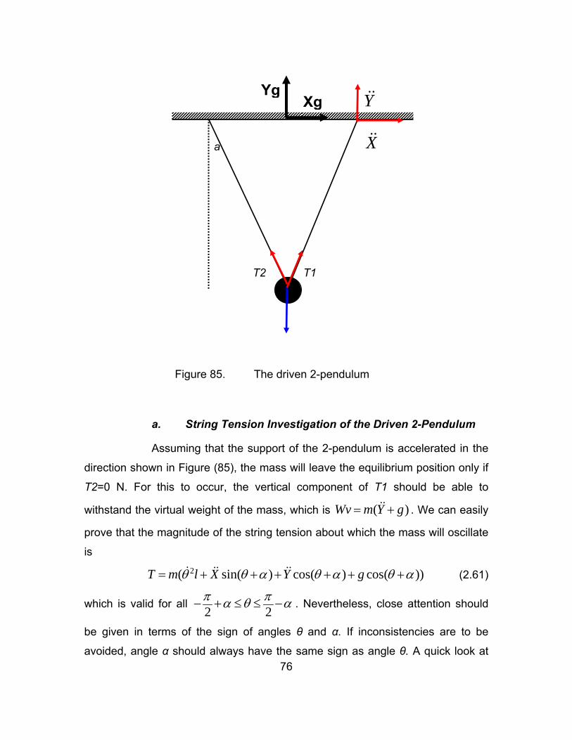
76
Figure 85. The driven 2-pendulum
a. String Tension Investigation of the Driven 2-Pendulum
Assuming that the support of the 2-pendulum is accelerated in the
direction shown in Figure (85), the mass will leave the equilibrium position only if
T2=0 N. For this to occur, the vertical component of T1 should be able to
withstand the virtual weight of the mass, which is ( )Wv m Y g= + . We can easily
prove that the magnitude of the string tension about which the mass will oscillate
is
2( sin( ) cos( ) cos( ))θ θ α θ α θ α= + + + + + +T m l X Y g (2.61)
which is valid for all 2 2π πα θ α− + ≤ ≤ − . Nevertheless, close attention should
be given in terms of the sign of angles θ and α. If inconsistencies are to be
avoided, angle α should always have the same sign as angle θ. A quick look at
a
T1 T2
X
YYgXg
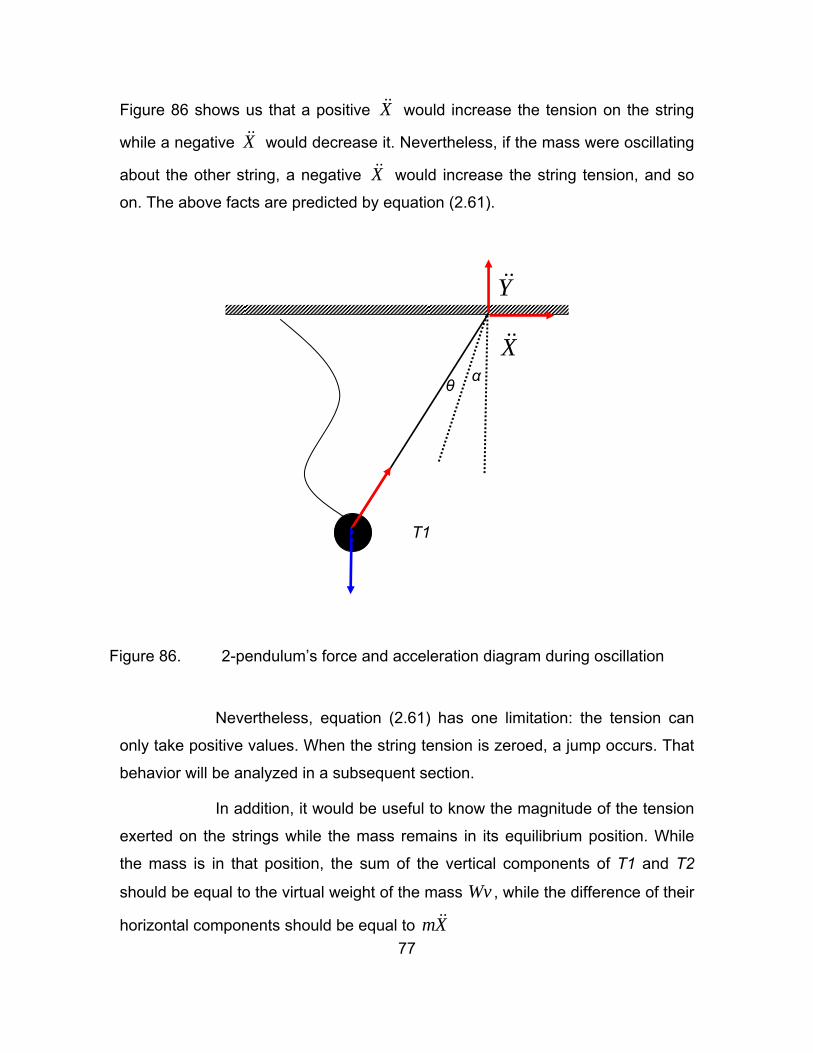
77
Figure 86 shows us that a positive X would increase the tension on the string
while a negative X would decrease it. Nevertheless, if the mass were oscillating
about the other string, a negative X would increase the string tension, and so
on. The above facts are predicted by equation (2.61).
Figure 86. 2-pendulum’s force and acceleration diagram during oscillation
Nevertheless, equation (2.61) has one limitation: the tension can
only take positive values. When the string tension is zeroed, a jump occurs. That
behavior will be analyzed in a subsequent section.
In addition, it would be useful to know the magnitude of the tension
exerted on the strings while the mass remains in its equilibrium position. While
the mass is in that position, the sum of the vertical components of T1 and T2
should be equal to the virtual weight of the mass Wv , while the difference of their
horizontal components should be equal to mX
α
T1 T2
X
Y
θ
78
cos ( 1 2) ( )T T m Y gα + = + and sin ( 1 2)T T mXα − =
solving the above system of two equations
( )1 ( )2 cos sin
( )2 ( )2 cos sin
α α
α α
+= +
+= −
m Y g XT
m Y g XT (2.62)
b. Stability of the 2-Pendulum
While equation (2.60) describes the 2-pendulum’s oscillation in the
absence of non-zero initial conditions, the oscillation will not be initiated under
any value of horizontal acceleration.
Manipulating equation (2.60) with zero initial conditions, results in
( ) sin cosg Y Xl l
θ α α+= − + . The vertical components of the restoring force
tend to drive the mass to move downwards. This motion is constrained in this
situation since the mass is supported by both the taught string (an exception
exists for the case that Y is negative and 0g Y+ < ). Therefore, an angular
acceleration will be induced only if the horizontal component manages to
overcome the condition and
tanα
− >X
Y g (2.63)
is fulfilled.
Another approach, which would lead us to the same conclusion, is
analyzing the string tension. Assuming that the support of the 2-pendulum is
accelerated in the direction shown in Figure 86, the mass will leave the
equilibrium position only if T2=0 N. For this to occur, the vertical component of T1
should be able to withstand the virtual weight of the mass, which is
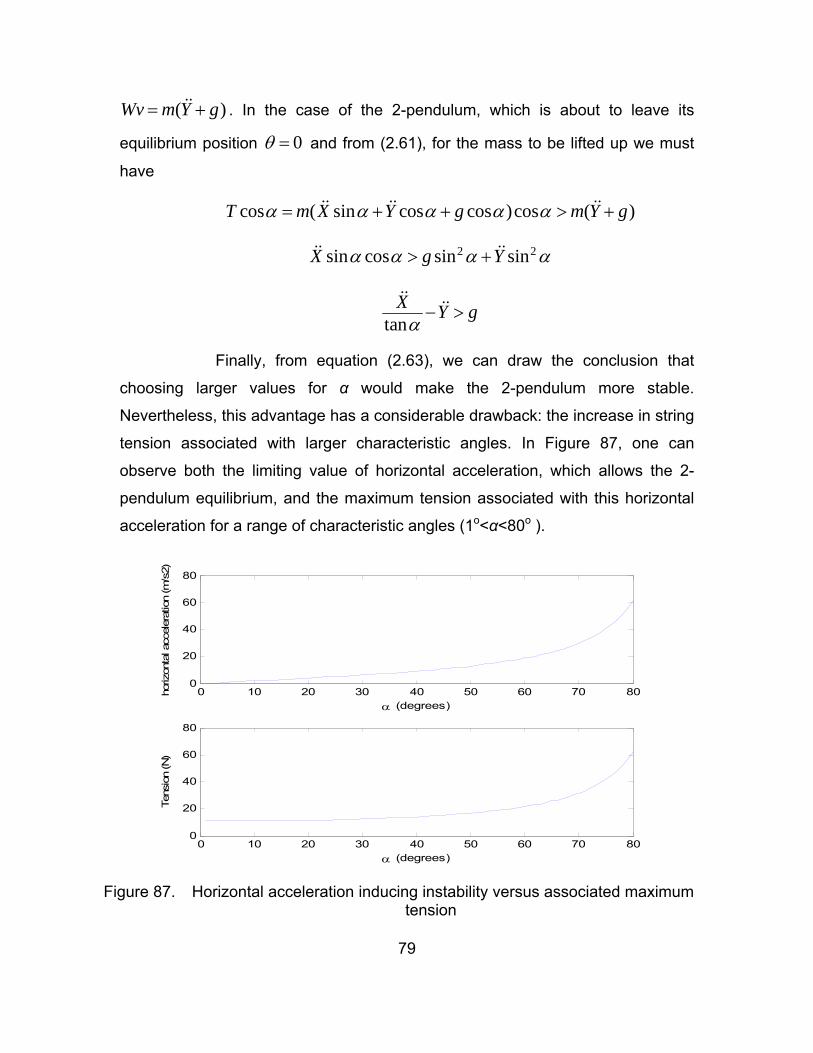
79
( )Wv m Y g= + . In the case of the 2-pendulum, which is about to leave its
equilibrium position 0θ = and from (2.61), for the mass to be lifted up we must
have
cos ( sin cos cos )cos ( )T m X Y g m Y gα α α α α= + + > +
2 2sin cos sin sinX g Yα α α α> +
tanX Y gα− >
Finally, from equation (2.63), we can draw the conclusion that
choosing larger values for α would make the 2-pendulum more stable.
Nevertheless, this advantage has a considerable drawback: the increase in string
tension associated with larger characteristic angles. In Figure 87, one can
observe both the limiting value of horizontal acceleration, which allows the 2-
pendulum equilibrium, and the maximum tension associated with this horizontal
acceleration for a range of characteristic angles (1o<α<80o ).
0 10 20 30 40 50 60 70 800
20
40
60
80
α (degrees)
horiz
onta
l acc
eler
atio
n (m
/s2)
0 10 20 30 40 50 60 70 800
20
40
60
80
α (degrees)
Tens
ion
(N)
Figure 87. Horizontal acceleration inducing instability versus associated maximum
tension
80
From the above figure, it can be seen that, although the necessary
X would break the equilibrium, which increases steadily for the first half of the
range of α, the related tension increases in a slower pattern. This difference in
increasing pattern is caused by the analytical equations that describe them.
These equations are
lim min
max maxmax
( ) tan( )
cos sin
α
α α
= +
+= +
X g Yg Y XT
(2.64)
One method to evaluate the optimum choice of α would be to define
a ratio of acceleration over the maximum attained tension. According to the
previous equations, this ratio would be sinR α= .
Nevertheless, this method is not effective. The values of the
required X to disturb equilibrium are very large for the second half of the α
range, and even for some values of the first half. A more realistic approach is to
choose a value of α (for example 20o) as a reference value, αref, and, then,
compare the maximum tension, Tmaxref , with the one exerted on the strings of the
2-pendulums of larger α, but still associated with the same refX .
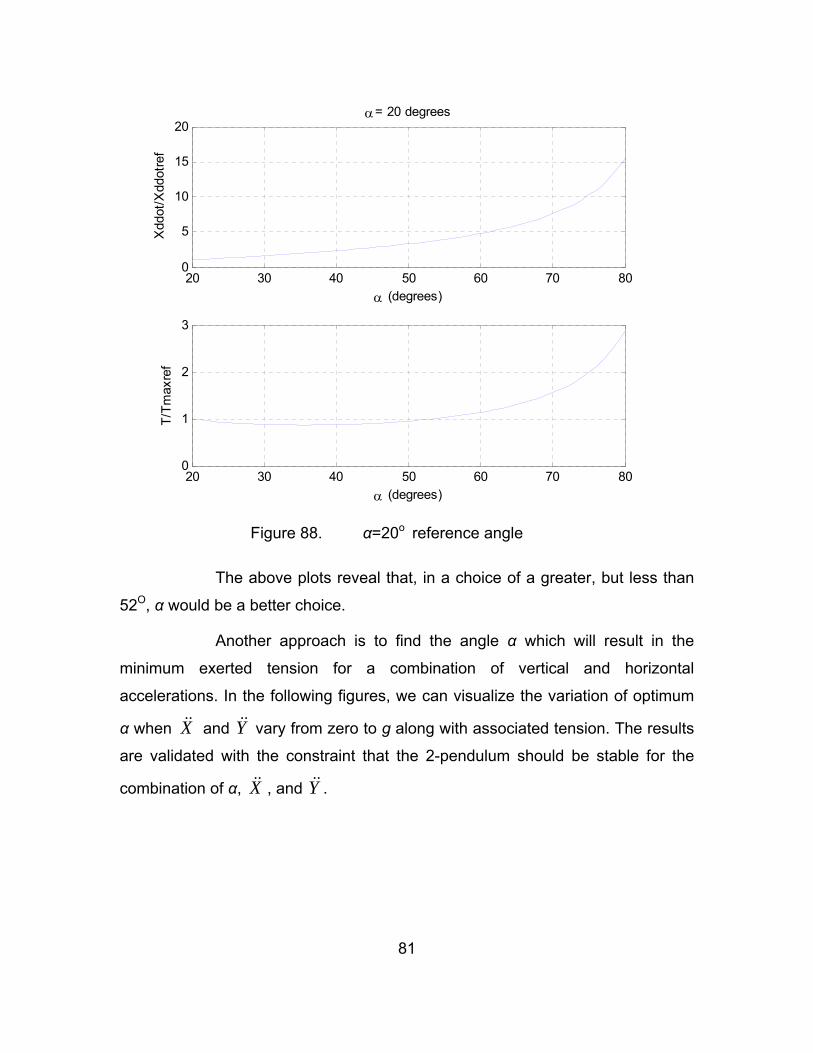
81
20 30 40 50 60 70 800
5
10
15
20
α (degrees)
Xdd
ot/X
ddot
ref
α= 20 degrees
20 30 40 50 60 70 800
1
2
3
α (degrees)
T/Tm
axre
f
Figure 88. α=20o reference angle
The above plots reveal that, in a choice of a greater, but less than
52O, α would be a better choice.
Another approach is to find the angle α which will result in the
minimum exerted tension for a combination of vertical and horizontal
accelerations. In the following figures, we can visualize the variation of optimum
α when X and Y vary from zero to g along with associated tension. The results
are validated with the constraint that the 2-pendulum should be stable for the
combination of α, X , and Y .
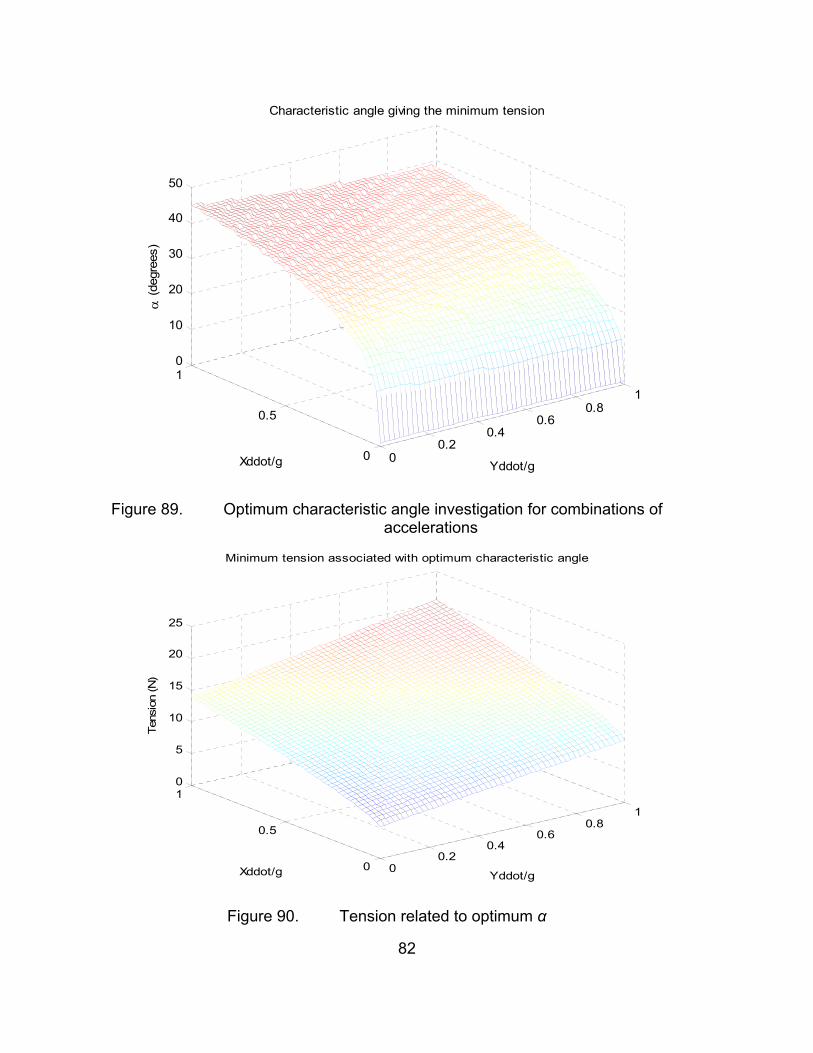
82
00.2
0.40.6
0.81
0
0.5
10
10
20
30
40
50
Yddot/g
Characteristic angle giving the minimum tension
Xddot/g
α (d
egre
es)
Figure 89. Optimum characteristic angle investigation for combinations of
accelerations
00.2
0.40.6
0.81
0
0.5
10
5
10
15
20
25
Yddot/g
Minimum tension associated with optimum characteristic angle
Xddot/g
Tens
ion
(N)
Figure 90. Tension related to optimum α
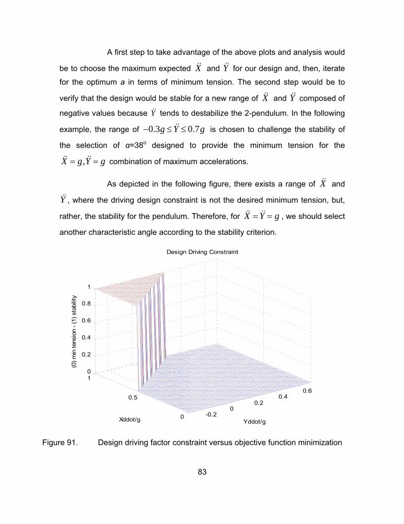
83
A first step to take advantage of the above plots and analysis would
be to choose the maximum expected X and Y for our design and, then, iterate
for the optimum a in terms of minimum tension. The second step would be to
verify that the design would be stable for a new range of X and Y composed of
negative values because Y tends to destabilize the 2-pendulum. In the following
example, the range of 0.3 0.7g Y g− ≤ ≤ is chosen to challenge the stability of
the selection of α=38o designed to provide the minimum tension for the
,X g Y g= = combination of maximum accelerations.
As depicted in the following figure, there exists a range of X and
Y , where the driving design constraint is not the desired minimum tension, but,
rather, the stability for the pendulum. Therefore, for X Y g= = , we should select
another characteristic angle according to the stability criterion.
-0.20
0.20.4
0.6
0
0.5
10
0.2
0.4
0.6
0.8
1
Yddot/g
Design Driving Constraint
Xddot/g
(0) m
in te
nsio
n - (
1) s
tabi
lity
Figure 91. Design driving factor constraint versus objective function minimization
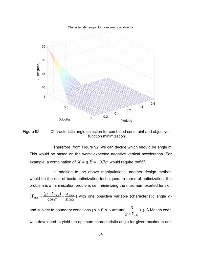
84
-0.20
0.20.4
0.6
0
0.5
1
40
45
50
55
Yddot/g
Characteristic angle for combined constraints
Xddot/g
α (d
egre
es)
Figure 92. Characteristic angle selection for combined constraint and objective
function minimization
Therefore, from Figure 92, we can decide which should be angle α.
This would be based on the worst expected negative vertical acceleration. For
example, a combination of , 0.3X g Y g= = − would require α=55o.
In addition to the above manipulations, another design method
would be the use of basic optimization techniques. In terms of optimization, the
problem is a minimization problem, i.e., minimizing the maximum exerted tension
( max maxmax
( )cos sin
g Y XTα α
+= + ) with one objective variable (characteristic angle α)
and subject to boundary conditions (min
0, arctan( )Xg Y
α α> >+
). A Matlab code
was developed to yield the optimum characteristic angle for given maximum and
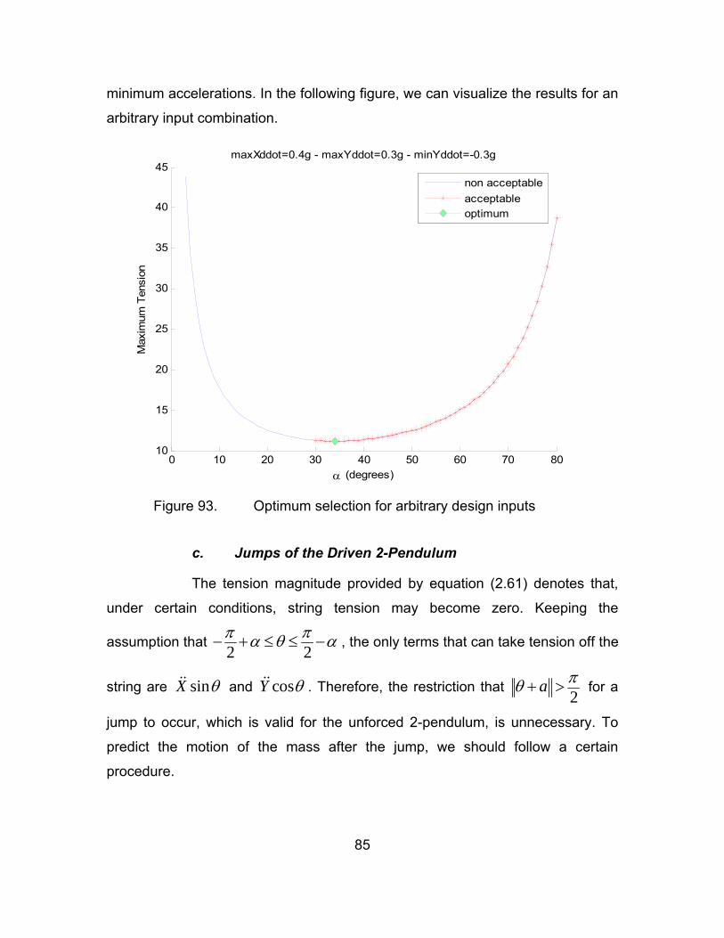
85
minimum accelerations. In the following figure, we can visualize the results for an
arbitrary input combination.
0 10 20 30 40 50 60 70 8010
15
20
25
30
35
40
45
α (degrees)
Max
imum
Ten
sion
maxXddot=0.4g - maxYddot=0.3g - minYddot=-0.3g
non acceptableacceptableoptimum
Figure 93. Optimum selection for arbitrary design inputs
c. Jumps of the Driven 2-Pendulum
The tension magnitude provided by equation (2.61) denotes that,
under certain conditions, string tension may become zero. Keeping the
assumption that 2 2π πα θ α− + ≤ ≤ − , the only terms that can take tension off the
string are sinX θ and cosY θ . Therefore, the restriction that 2
a πθ + > for a
jump to occur, which is valid for the unforced 2-pendulum, is unnecessary. To
predict the motion of the mass after the jump, we should follow a certain
procedure.
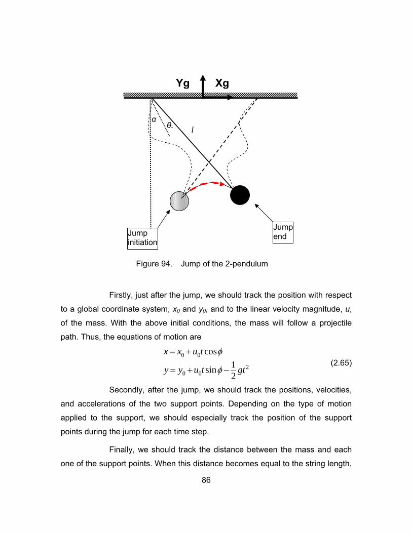
86
Figure 94. Jump of the 2-pendulum
Firstly, just after the jump, we should track the position with respect
to a global coordinate system, x0 and y0, and to the linear velocity magnitude, u,
of the mass. With the above initial conditions, the mass will follow a projectile
path. Thus, the equations of motion are
0 0
20 0
cos1sin2
x x u t
y y u t gt
φ
φ
= +
= + − (2.65)
Secondly, after the jump, we should track the positions, velocities,
and accelerations of the two support points. Depending on the type of motion
applied to the support, we should especially track the position of the support
points during the jump for each time step.
Finally, we should track the distance between the mass and each
one of the support points. When this distance becomes equal to the string length,
θ-α
l
Jump initiation
Jumpend
XgYg
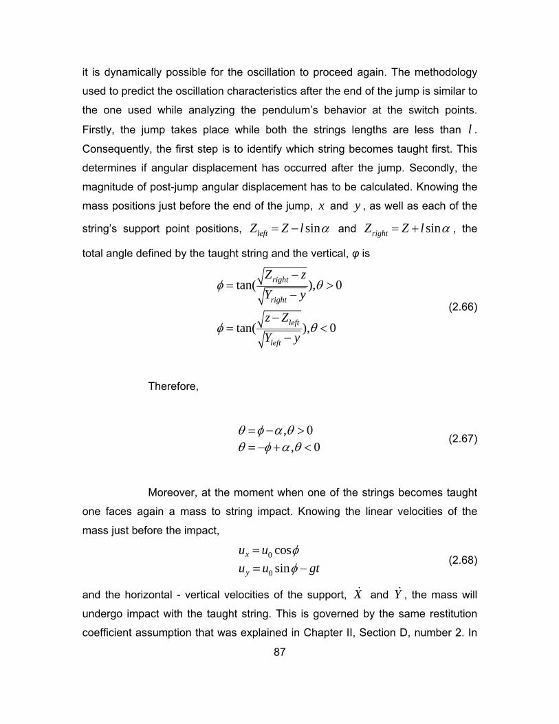
87
it is dynamically possible for the oscillation to proceed again. The methodology
used to predict the oscillation characteristics after the end of the jump is similar to
the one used while analyzing the pendulum’s behavior at the switch points.
Firstly, the jump takes place while both the strings lengths are less than l .
Consequently, the first step is to identify which string becomes taught first. This
determines if angular displacement has occurred after the jump. Secondly, the
magnitude of post-jump angular displacement has to be calculated. Knowing the
mass positions just before the end of the jump, x and y , as well as each of the
string’s support point positions, sinleftZ Z l α= − and sinrightZ Z l α= + , the
total angle defined by the taught string and the vertical, φ is
tan( ), 0
tan( ), 0
φ θ
φ θ
−= >
−
−= <
−
right
right
left
left
Z zY y
z ZY y
(2.66)
Therefore,
, 0
, 0θ φ α θθ φ α θ= − >= − + <
(2.67)
Moreover, at the moment when one of the strings becomes taught
one faces again a mass to string impact. Knowing the linear velocities of the
mass just before the impact,
0
0
cossin
φφ
== −
x
y
u uu u gt
(2.68)
and the horizontal - vertical velocities of the support, X and Y , the mass will
undergo impact with the taught string. This is governed by the same restitution
coefficient assumption that was explained in Chapter II, Section D, number 2. In
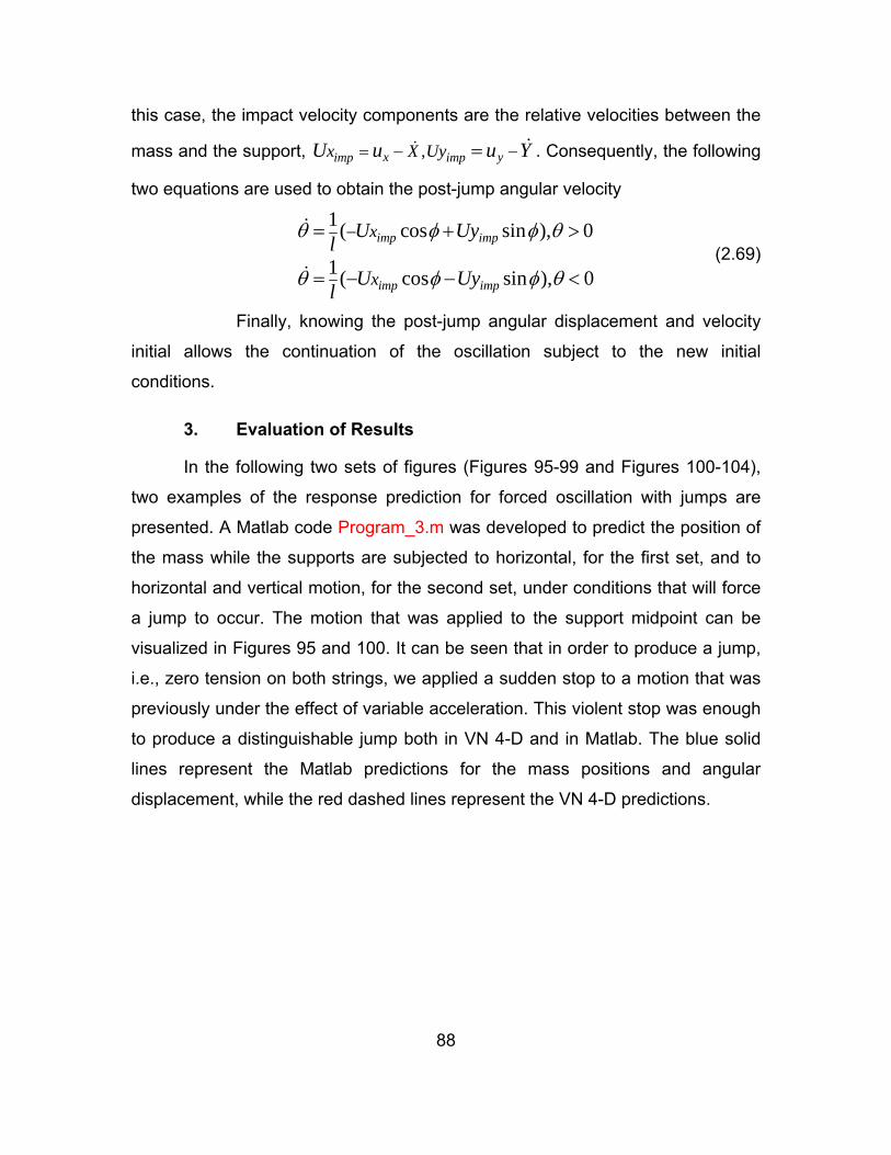
88
this case, the impact velocity components are the relative velocities between the
mass and the support, ,x yimp impx X UyU u u Y= − −= . Consequently, the following
two equations are used to obtain the post-jump angular velocity
1( cos sin ), 0
1( cos sin ), 0
θ φ φ θ
θ φ φ θ
−= + >
= − − <
imp imp
imp imp
x
x
U Uyl
U Uyl
(2.69)
Finally, knowing the post-jump angular displacement and velocity
initial allows the continuation of the oscillation subject to the new initial
conditions.
3. Evaluation of Results
In the following two sets of figures (Figures 95-99 and Figures 100-104),
two examples of the response prediction for forced oscillation with jumps are
presented. A Matlab code Program_3.m was developed to predict the position of
the mass while the supports are subjected to horizontal, for the first set, and to
horizontal and vertical motion, for the second set, under conditions that will force
a jump to occur. The motion that was applied to the support midpoint can be
visualized in Figures 95 and 100. It can be seen that in order to produce a jump,
i.e., zero tension on both strings, we applied a sudden stop to a motion that was
previously under the effect of variable acceleration. This violent stop was enough
to produce a distinguishable jump both in VN 4-D and in Matlab. The blue solid
lines represent the Matlab predictions for the mass positions and angular
displacement, while the red dashed lines represent the VN 4-D predictions.
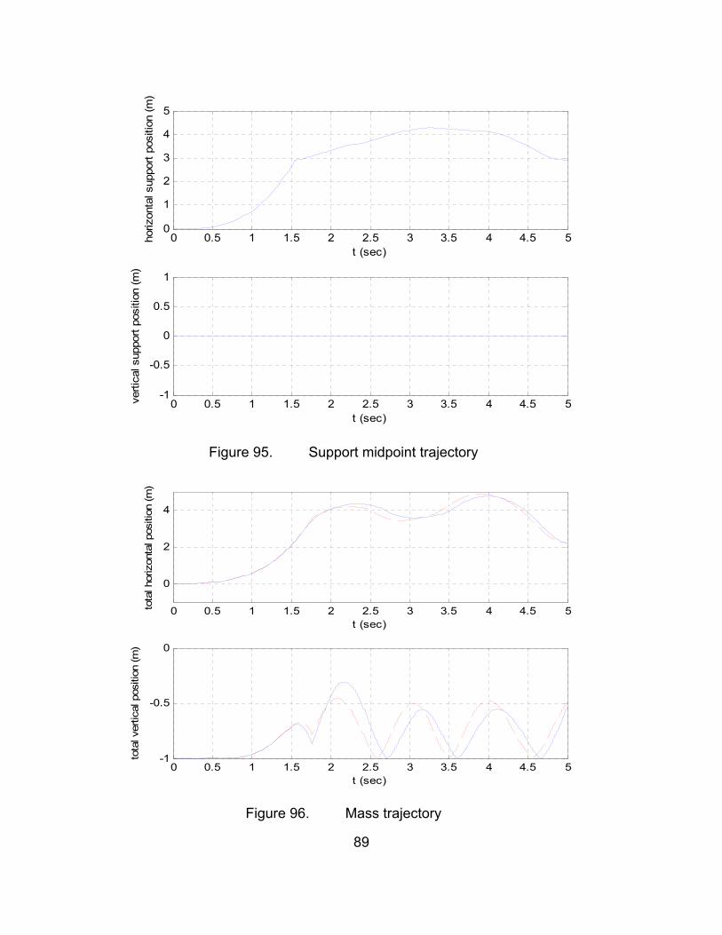
89
0 0.5 1 1.5 2 2.5 3 3.5 4 4.5 50
1
2
3
4
5
t (sec)
hor
izon
tal s
uppo
rt po
sitio
n (m
)
0 0.5 1 1.5 2 2.5 3 3.5 4 4.5 5-1
-0.5
0
0.5
1
t (sec)
verti
cal s
uppo
rt po
sitio
n (m
)
Figure 95. Support midpoint trajectory
0 0.5 1 1.5 2 2.5 3 3.5 4 4.5 5
0
2
4
t (sec)
tota
l hor
izon
tal p
ositi
on (m
)
0 0.5 1 1.5 2 2.5 3 3.5 4 4.5 5-1
-0.5
0
t (sec)
tota
l ver
tical
pos
ition
(m)
Figure 96. Mass trajectory
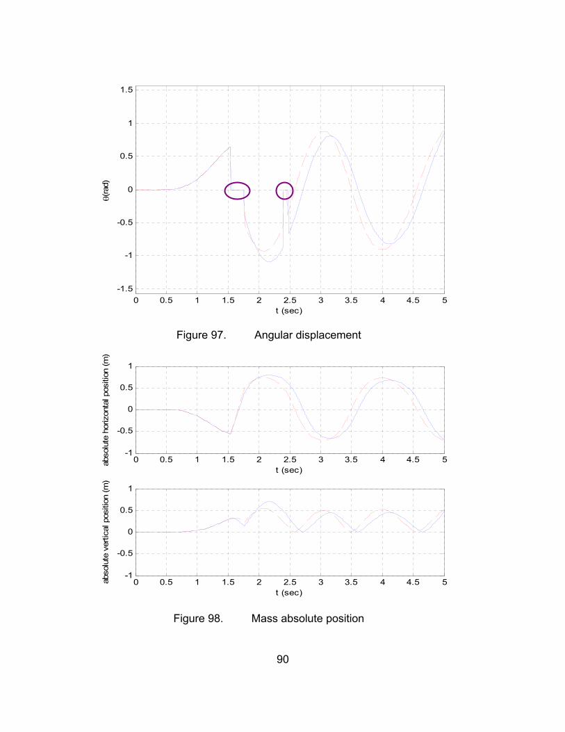
90
0 0.5 1 1.5 2 2.5 3 3.5 4 4.5 5-1.5
-1
-0.5
0
0.5
1
1.5
t (sec)
θ(ra
d)
Figure 97. Angular displacement
0 0.5 1 1.5 2 2.5 3 3.5 4 4.5 5-1
-0.5
0
0.5
1
t (sec)
abso
lute
hor
izon
tal p
ositi
on (m
)
0 0.5 1 1.5 2 2.5 3 3.5 4 4.5 5-1
-0.5
0
0.5
1
t (sec)
abso
lute
ver
tical
pos
ition
(m)
Figure 98. Mass absolute position
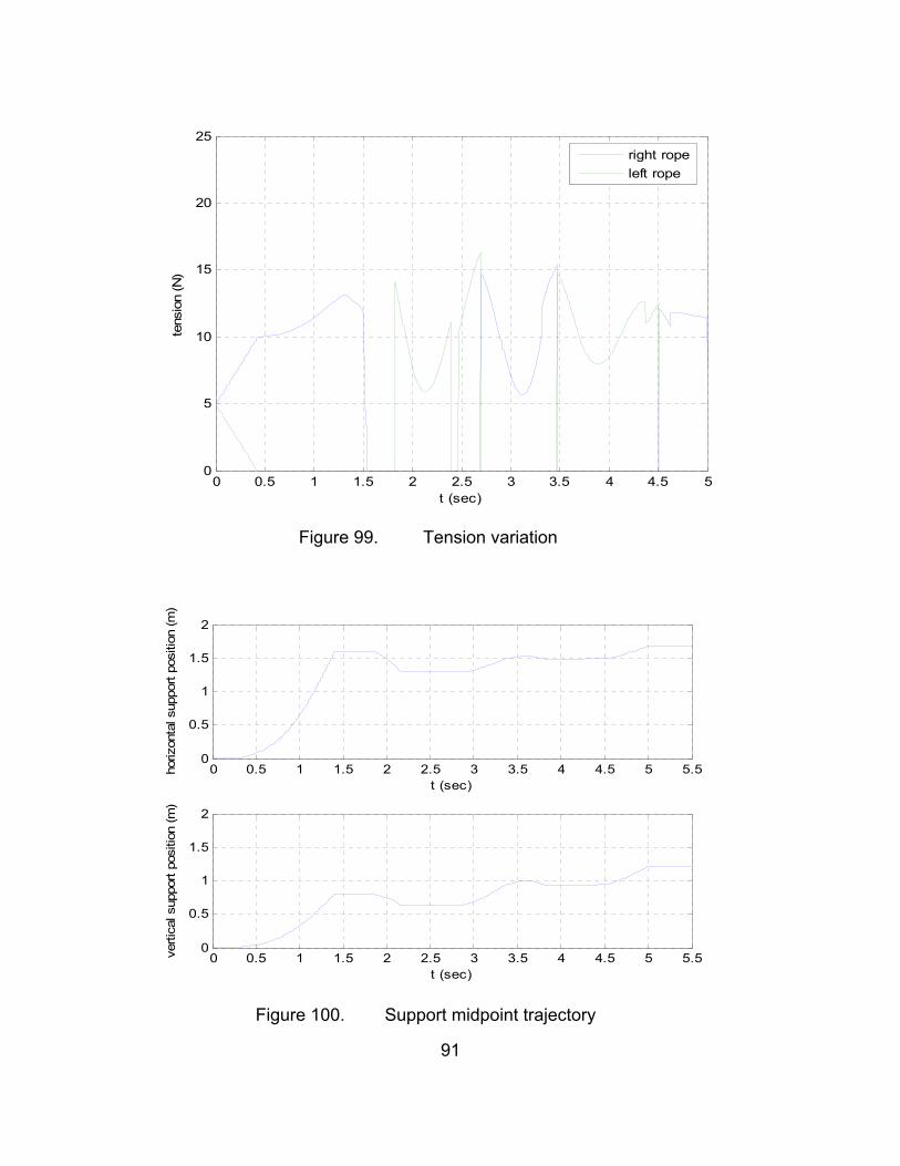
91
0 0.5 1 1.5 2 2.5 3 3.5 4 4.5 50
5
10
15
20
25
t (sec)
tens
ion
(N)
right ropeleft rope
Figure 99. Tension variation
0 0.5 1 1.5 2 2.5 3 3.5 4 4.5 5 5.50
0.5
1
1.5
2
t (sec)
hor
izon
tal s
uppo
rt po
sitio
n (m
)
0 0.5 1 1.5 2 2.5 3 3.5 4 4.5 5 5.50
0.5
1
1.5
2
t (sec)
verti
cal s
uppo
rt po
sitio
n (m
)
Figure 100. Support midpoint trajectory
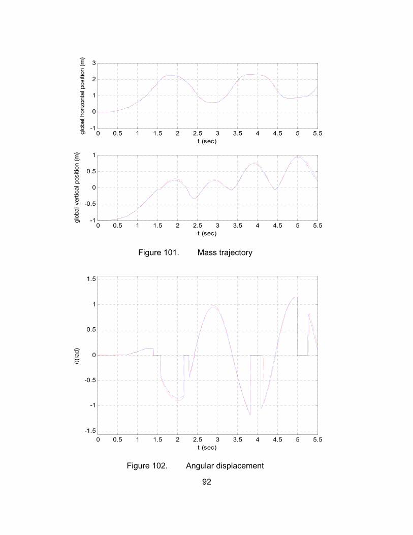
92
0 0.5 1 1.5 2 2.5 3 3.5 4 4.5 5 5.5-1
0
1
2
3
t (sec)
glob
al h
oriz
onta
l pos
ition
(m)
0 0.5 1 1.5 2 2.5 3 3.5 4 4.5 5 5.5-1
-0.5
0
0.5
1
t (sec)
glob
al v
ertic
al p
ositi
on (m
)
Figure 101. Mass trajectory
0 0.5 1 1.5 2 2.5 3 3.5 4 4.5 5 5.5-1.5
-1
-0.5
0
0.5
1
1.5
t (sec)
θ(ra
d)
Figure 102. Angular displacement
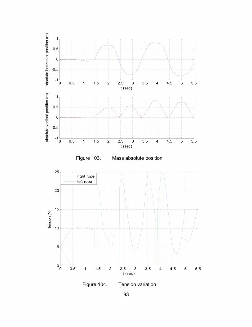
93
0 0.5 1 1.5 2 2.5 3 3.5 4 4.5 5 5.5-1
-0.5
0
0.5
1
t (sec)
abso
lute
hor
izon
tal p
ositi
on (m
)
0 0.5 1 1.5 2 2.5 3 3.5 4 4.5 5 5.5-1
-0.5
0
0.5
1
t (sec)
abso
lute
ver
tical
pos
ition
(m)
Figure 103. Mass absolute position
0 0.5 1 1.5 2 2.5 3 3.5 4 4.5 5 5.50
5
10
15
20
25
t (sec)
tens
ion
(N)
right ropeleft rope
Figure 104. Tension variation
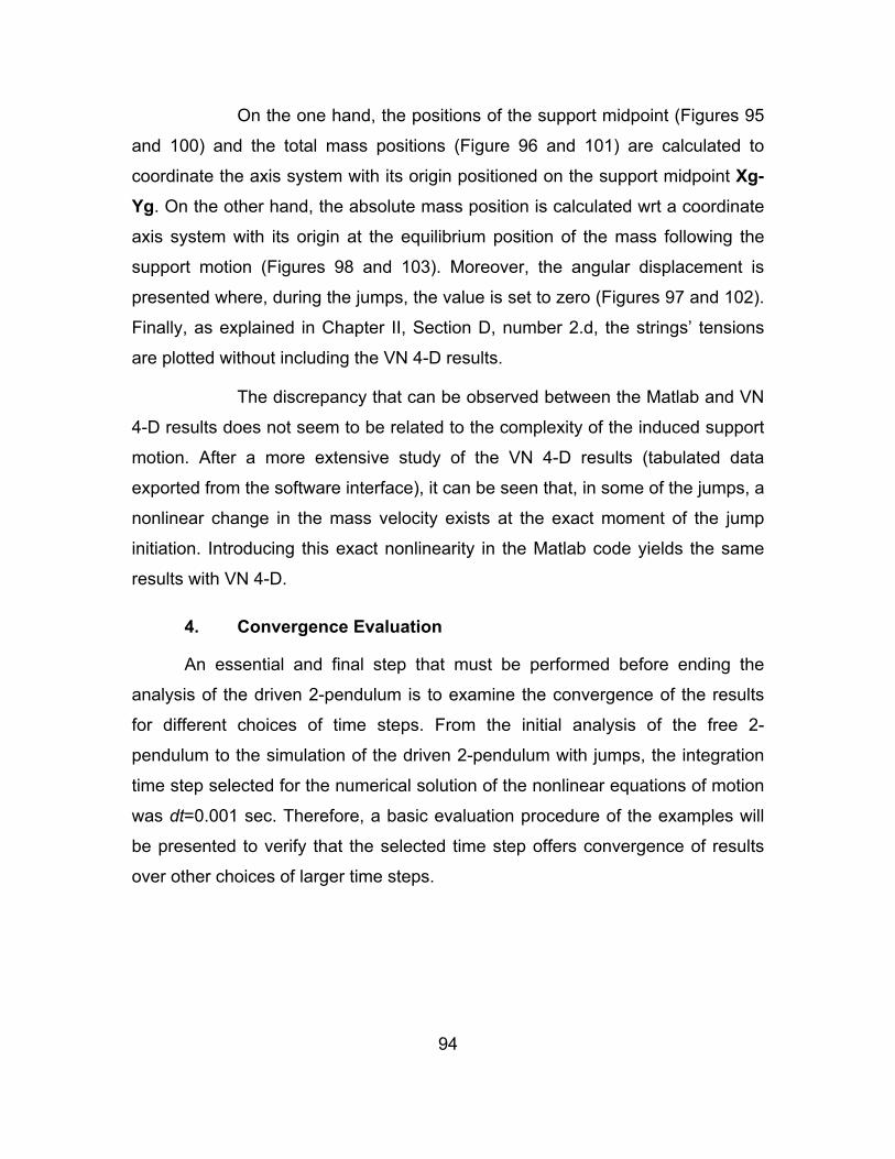
94
On the one hand, the positions of the support midpoint (Figures 95
and 100) and the total mass positions (Figure 96 and 101) are calculated to
coordinate the axis system with its origin positioned on the support midpoint Xg-Yg. On the other hand, the absolute mass position is calculated wrt a coordinate
axis system with its origin at the equilibrium position of the mass following the
support motion (Figures 98 and 103). Moreover, the angular displacement is
presented where, during the jumps, the value is set to zero (Figures 97 and 102).
Finally, as explained in Chapter II, Section D, number 2.d, the strings’ tensions
are plotted without including the VN 4-D results.
The discrepancy that can be observed between the Matlab and VN
4-D results does not seem to be related to the complexity of the induced support
motion. After a more extensive study of the VN 4-D results (tabulated data
exported from the software interface), it can be seen that, in some of the jumps, a
nonlinear change in the mass velocity exists at the exact moment of the jump
initiation. Introducing this exact nonlinearity in the Matlab code yields the same
results with VN 4-D.
4. Convergence Evaluation
An essential and final step that must be performed before ending the
analysis of the driven 2-pendulum is to examine the convergence of the results
for different choices of time steps. From the initial analysis of the free 2-
pendulum to the simulation of the driven 2-pendulum with jumps, the integration
time step selected for the numerical solution of the nonlinear equations of motion
was dt=0.001 sec. Therefore, a basic evaluation procedure of the examples will
be presented to verify that the selected time step offers convergence of results
over other choices of larger time steps.
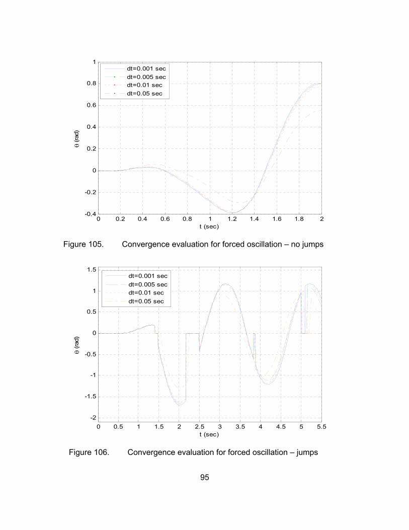
95
0 0.2 0.4 0.6 0.8 1 1.2 1.4 1.6 1.8 2-0.4
-0.2
0
0.2
0.4
0.6
0.8
1
t (sec)
θ (ra
d)dt=0.001 secdt=0.005 secdt=0.01 secdt=0.05 sec
Figure 105. Convergence evaluation for forced oscillation – no jumps
0 0.5 1 1.5 2 2.5 3 3.5 4 4.5 5 5.5-2
-1.5
-1
-0.5
0
0.5
1
1.5
t (sec)
θ (ra
d)
dt=0.001 secdt=0.005 secdt=0.01 secdt=0.05 sec
Figure 106. Convergence evaluation for forced oscillation – jumps

96
In Figure 105, the convergence is tested with both vertical and horizontal
support motion. A case with jumps is presented in Figure 106. From both figures,
one can easily conclude that gradually increasing the time step dt will provoke a
solution divergence. While the discrepancy for dt=0.005 sec or dt=0.01 sec (up to
ten times larger than the initial choice) will cause the solution to change slightly, a
further increase in the time step size may yield solutions with larger
discrepancies than the original. Especially in the jump cases, it can be seen that
some jumps are incorrectly predicted (in terms of time of jump initiation and
termination) or even skipped if the time step is large enough.
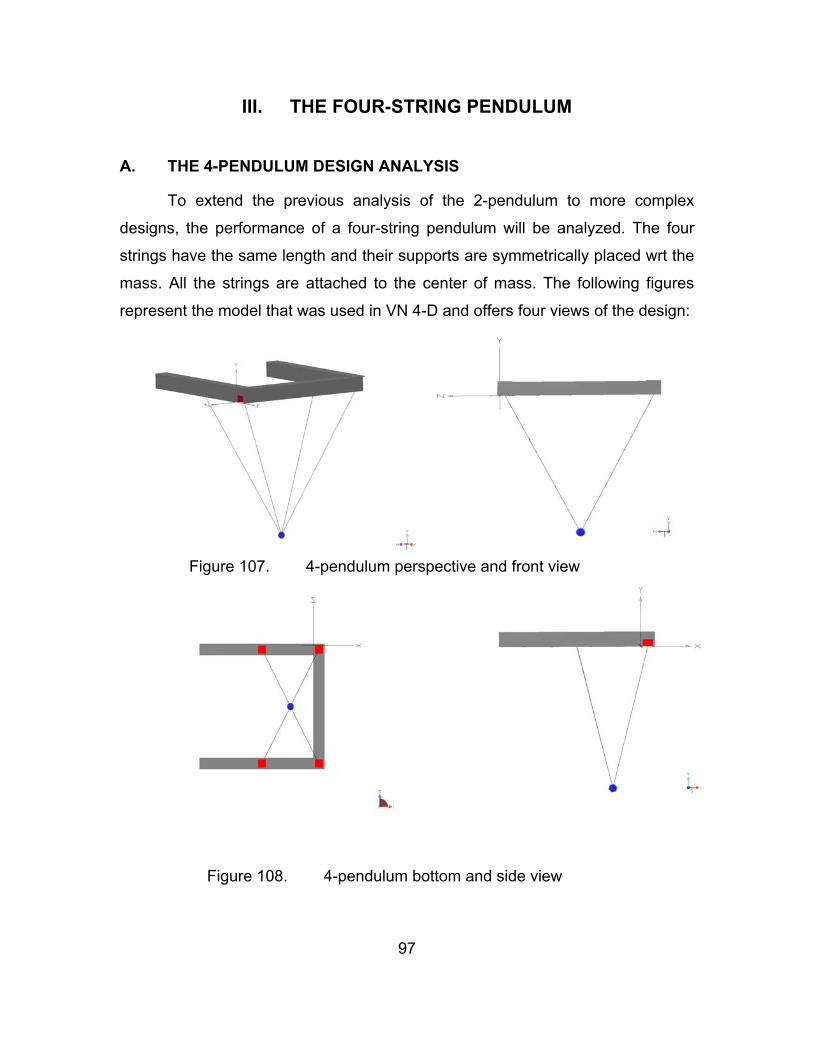
97
III. THE FOUR-STRING PENDULUM
A. THE 4-PENDULUM DESIGN ANALYSIS
To extend the previous analysis of the 2-pendulum to more complex
designs, the performance of a four-string pendulum will be analyzed. The four
strings have the same length and their supports are symmetrically placed wrt the
mass. All the strings are attached to the center of mass. The following figures
represent the model that was used in VN 4-D and offers four views of the design:
Figure 107. 4-pendulum perspective and front view
Figure 108. 4-pendulum bottom and side view
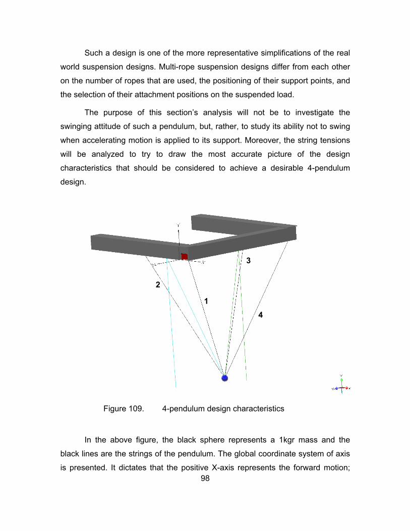
98
Such a design is one of the more representative simplifications of the real
world suspension designs. Multi-rope suspension designs differ from each other
on the number of ropes that are used, the positioning of their support points, and
the selection of their attachment positions on the suspended load.
The purpose of this section’s analysis will not be to investigate the
swinging attitude of such a pendulum, but, rather, to study its ability not to swing
when accelerating motion is applied to its support. Moreover, the string tensions
will be analyzed to try to draw the most accurate picture of the design
characteristics that should be considered to achieve a desirable 4-pendulum
design.
Figure 109. 4-pendulum design characteristics
In the above figure, the black sphere represents a 1kgr mass and the
black lines are the strings of the pendulum. The global coordinate system of axis
is presented. It dictates that the positive X-axis represents the forward motion;
1
2
3
4
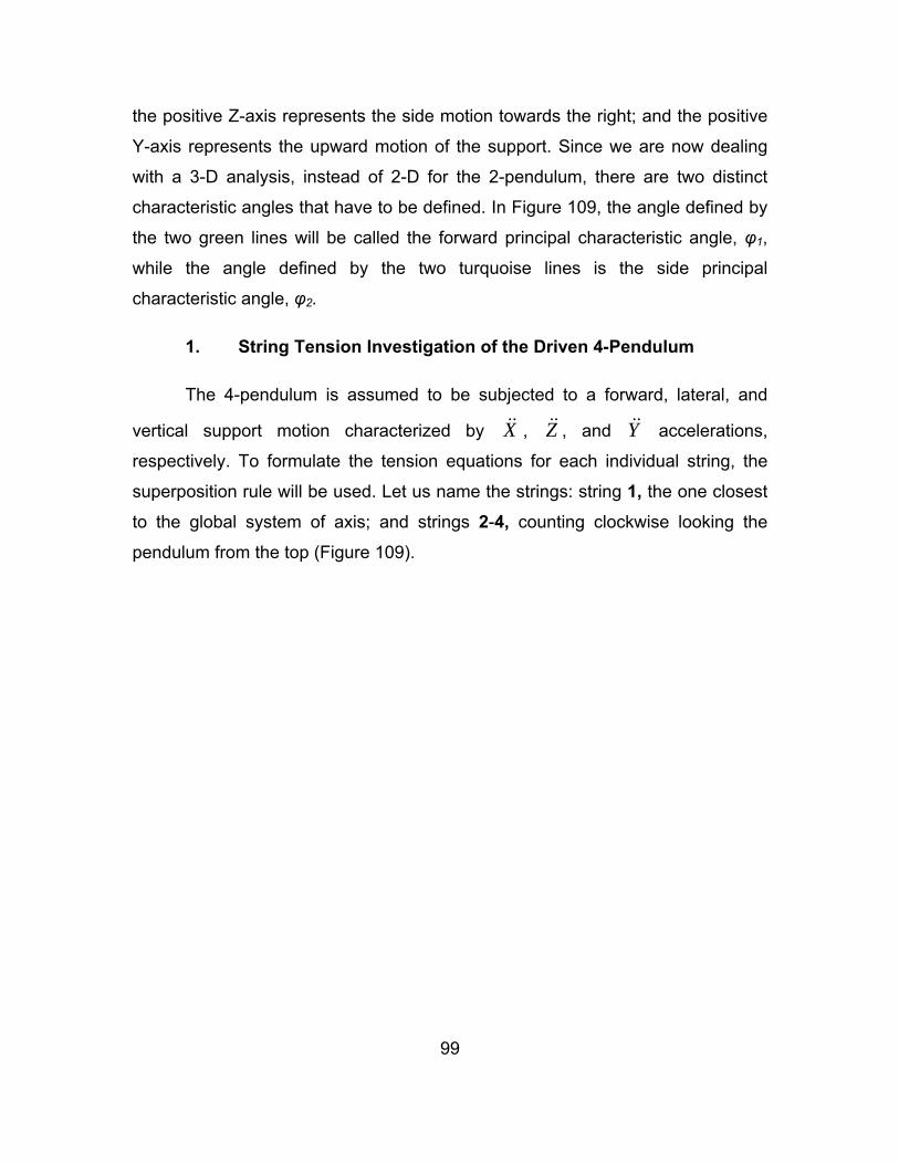
99
the positive Z-axis represents the side motion towards the right; and the positive
Y-axis represents the upward motion of the support. Since we are now dealing
with a 3-D analysis, instead of 2-D for the 2-pendulum, there are two distinct
characteristic angles that have to be defined. In Figure 109, the angle defined by
the two green lines will be called the forward principal characteristic angle, φ1,
while the angle defined by the two turquoise lines is the side principal
characteristic angle, φ2.
1. String Tension Investigation of the Driven 4-Pendulum
The 4-pendulum is assumed to be subjected to a forward, lateral, and
vertical support motion characterized by X , Z , and Y accelerations,
respectively. To formulate the tension equations for each individual string, the
superposition rule will be used. Let us name the strings: string 1, the one closest
to the global system of axis; and strings 2-4, counting clockwise looking the
pendulum from the top (Figure 109).
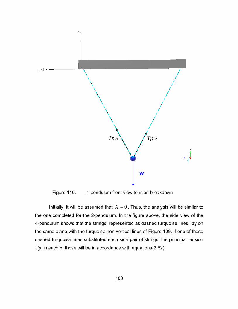
100
Figure 110. 4-pendulum front view tension breakdown
Initially, it will be assumed that 0X = . Thus, the analysis will be similar to
the one completed for the 2-pendulum. In the figure above, the side view of the
4-pendulum shows that the strings, represented as dashed turquoise lines, lay on
the same plane with the turquoise non vertical lines of Figure 109. If one of these
dashed turquoise lines substituted each side pair of strings, the principal tension
Tp in each of those will be in accordance with equations(2.62).
21Tp 22Tp
W
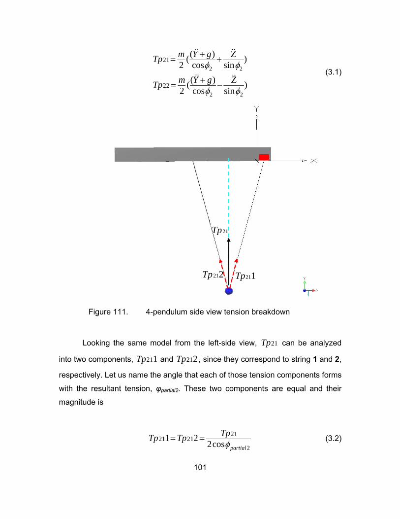
101
2 2
2 2
21
22
( )( )2 cos sin
( )( )2 cos sin
φ φ
φ φ
+ Ζ= +
+ Ζ= −
m Y gTp
m Y gTp (3.1)
Figure 111. 4-pendulum side view tension breakdown
Looking the same model from the left-side view, 21Tp can be analyzed
into two components, 211Tp and 212Tp , since they correspond to string 1 and 2,
respectively. Let us name the angle that each of those tension components forms
with the resultant tension, φpartial2. These two components are equal and their
magnitude is
2
2121 211 2
2cosφ= =
partial
TpTp Tp (3.2)
21Tp
211Tp 212Tp
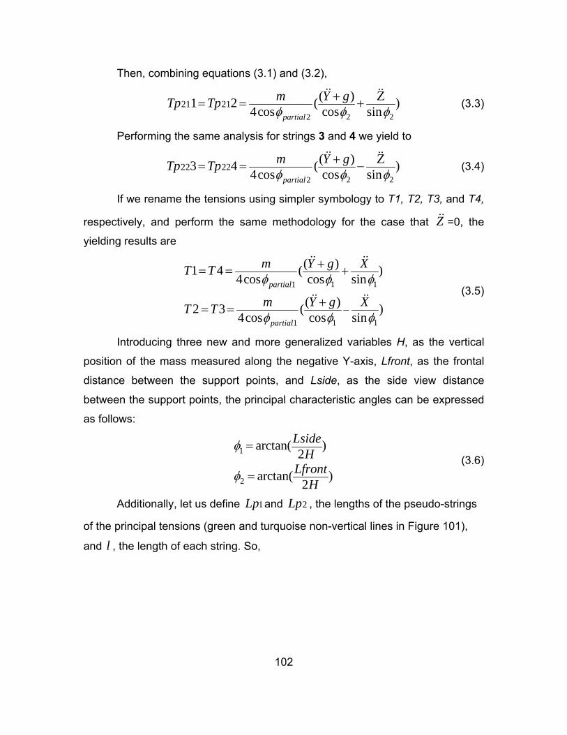
102
Then, combining equations (3.1) and (3.2),
2 22
21 21( )1 2 ( )
4cos cos sinφ φ φ+ Ζ= = +
partial
m Y gTp Tp (3.3)
Performing the same analysis for strings 3 and 4 we yield to
2 22
22 22( )3 4 ( )
4cos cos sinφ φ φ+ Ζ= = −
partial
m Y gTp Tp (3.4)
If we rename the tensions using simpler symbology to T1, T2, T3, and T4,
respectively, and perform the same methodology for the case that Z =0, the
yielding results are
1 11
1 11
( )1 4 ( )4cos cos sin
( )2 3 ( )4cos cos sin
φ φ φ
φ φ φ−
+= = +
+= =
partial
partial
m Y g XT T
m Y g XT T (3.5)
Introducing three new and more generalized variables H, as the vertical
position of the mass measured along the negative Y-axis, Lfront, as the frontal
distance between the support points, and Lside, as the side view distance
between the support points, the principal characteristic angles can be expressed
as follows:
1
2
arctan( )2
arctan( )2
LsideH
LfrontH
φ
φ
=
= (3.6)
Additionally, let us define 1Lp and 2Lp , the lengths of the pseudo-strings
of the principal tensions (green and turquoise non-vertical lines in Figure 101),
and l , the length of each string. So,
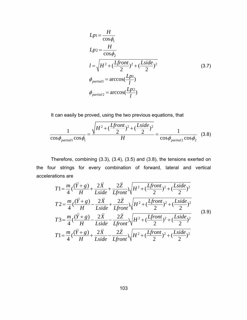
103
1
2
2 2 2
1
2
1
2
1
2
cos
cos
( ) ( )2 2
arccos( )
arccos( )
partial
partial
HLp
HLp
Lfront Lsidel H
Lpl
Lpl
φ
φ
φ
φ
=
=
= + +
=
=
(3.7)
It can easily be proved, using the two previous equations, that
2 2 2
1 21 2
( ) ( )1 12 2cos cos cos cospartial partial
Lfront LsideH
Hφ φ φ φ
+ += = (3.8)
Therefore, combining (3.3), (3.4), (3.5) and (3.8), the tensions exerted on
the four strings for every combination of forward, lateral and vertical
accelerations are
2 2 2
2 2 2
2 2 2
)
)
)
( ) 2 21 ( ( ) ( )4 2 2
( ) 2 22 ( ( ) ( )4 2 2
( ) 2 23 ( ( ) ( )4 2 2
( ) 21 (4
+= + + + +
+= − + + +
+= − − + +
+= +
m Y g X Z Lfront LsideT HH Lside Lfront
m Y g X Z Lfront LsideT HH Lside Lfront
m Y g X Z Lfront LsideT HH Lside Lfront
m Y g XTH Lsid
2 2 2)2 ( ) ( )2 2
− + +Z Lfront LsideHe Lfront
(3.9)
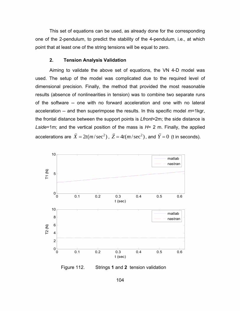
104
This set of equations can be used, as already done for the corresponding
one of the 2-pendulum, to predict the stability of the 4-pendulum, i.e., at which
point that at least one of the string tensions will be equal to zero.
2. Tension Analysis Validation
Aiming to validate the above set of equations, the VN 4-D model was
used. The setup of the model was complicated due to the required level of
dimensional precision. Finally, the method that provided the most reasonable
results (absence of nonlinearities in tension) was to combine two separate runs
of the software -- one with no forward acceleration and one with no lateral
acceleration -- and then superimpose the results. In this specific model m=1kgr,
the frontal distance between the support points is Lfront=2m; the side distance is
Lside=1m; and the vertical position of the mass is H= 2 m. Finally, the applied
accelerations are 22 ( / sec )X t m= , 24 ( / sec )Z t m= , and 0Y = (t in seconds).
0 0.1 0.2 0.3 0.4 0.5 0.60
5
10
t (sec)
T1 (N
)
matlabnastran
0 0.1 0.2 0.3 0.4 0.5 0.60
2
4
6
8
10
t (sec)
T2 (N
)
matlabnastran
Figure 112. Strings 1 and 2 tension validation
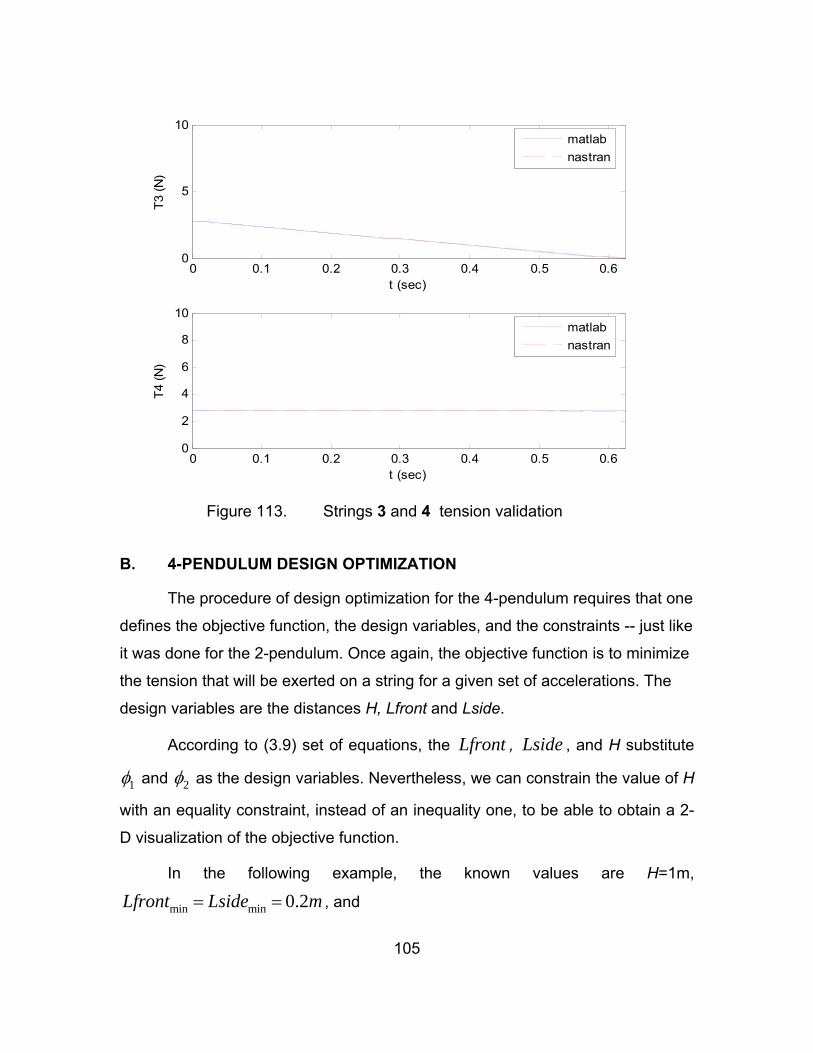
105
0 0.1 0.2 0.3 0.4 0.5 0.60
5
10
t (sec)
T3 (N
)
0 0.1 0.2 0.3 0.4 0.5 0.60
2
4
6
8
10
t (sec)
T4 (N
)matlabnastran
matlabnastran
Figure 113. Strings 3 and 4 tension validation
B. 4-PENDULUM DESIGN OPTIMIZATION
The procedure of design optimization for the 4-pendulum requires that one
defines the objective function, the design variables, and the constraints -- just like
it was done for the 2-pendulum. Once again, the objective function is to minimize
the tension that will be exerted on a string for a given set of accelerations. The
design variables are the distances H, Lfront and Lside.
According to (3.9) set of equations, the Lfront , Lside , and H substitute
1φ and 2φ as the design variables. Nevertheless, we can constrain the value of H
with an equality constraint, instead of an inequality one, to be able to obtain a 2-
D visualization of the objective function.
In the following example, the known values are H=1m,
min min 0.2Lfront Lside m= = , and
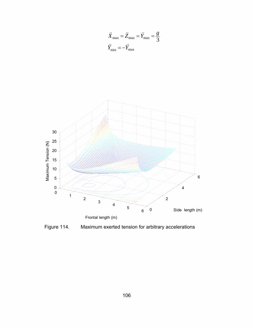
106
max max max
maxmin
3gX Z Y
Y Y
= = =
= −
01
23
45
6 0
2
4
6
0
5
10
15
20
25
30
Side length (m)
Frontal length (m)
Max
imum
Ten
sion
(N)
Figure 114. Maximum exerted tension for arbitrary accelerations
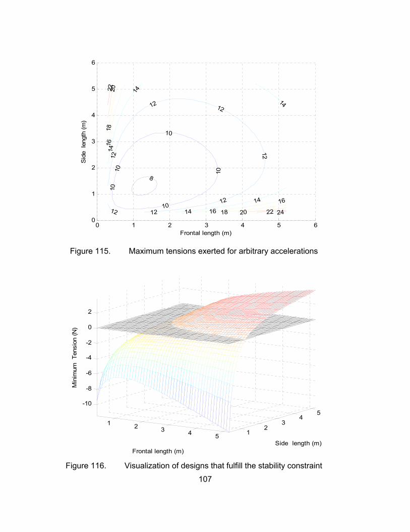
107
0 1 2 3 4 5 60
1
2
3
4
5
6
8
10
10
10
10
10
12 12
12
12
121212
14
14
14
14
1416
1616
18
18
20
20
22
22 24
Frontal length (m)
Sid
e le
ngth
(m)
Figure 115. Maximum tensions exerted for arbitrary accelerations
1 2 3 4 5 12
34
5-10
-8
-6
-4
-2
0
2
Side length (m)Frontal length (m)
Min
imum
Ten
sion
(N)
Figure 116. Visualization of designs that fulfill the stability constraint
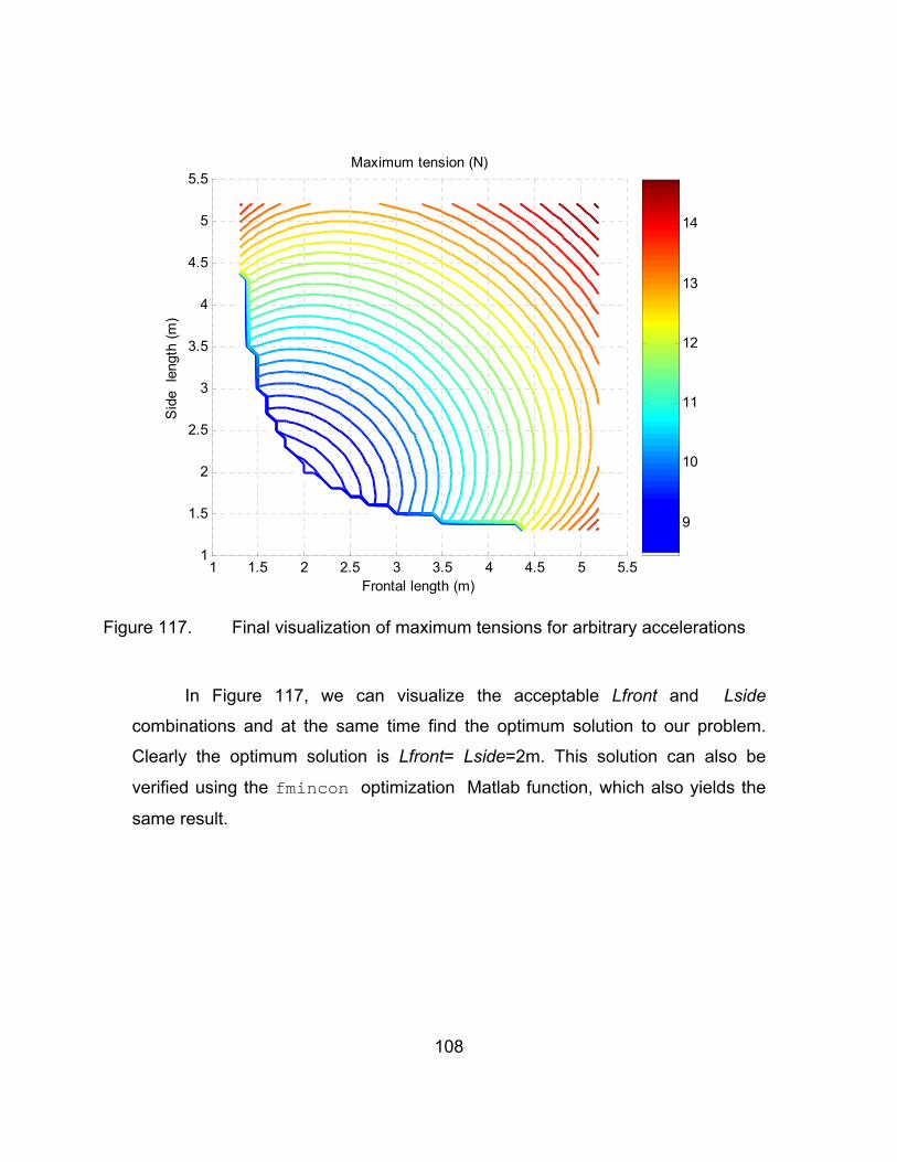
108
1 1.5 2 2.5 3 3.5 4 4.5 5 5.51
1.5
2
2.5
3
3.5
4
4.5
5
5.5
Frontal length (m)
Sid
e le
ngth
(m)
Maximum tension (N)
9
10
11
12
13
14
Figure 117. Final visualization of maximum tensions for arbitrary accelerations
In Figure 117, we can visualize the acceptable Lfront and Lside
combinations and at the same time find the optimum solution to our problem.
Clearly the optimum solution is Lfront= Lside=2m. This solution can also be
verified using the fmincon optimization Matlab function, which also yields the
same result.
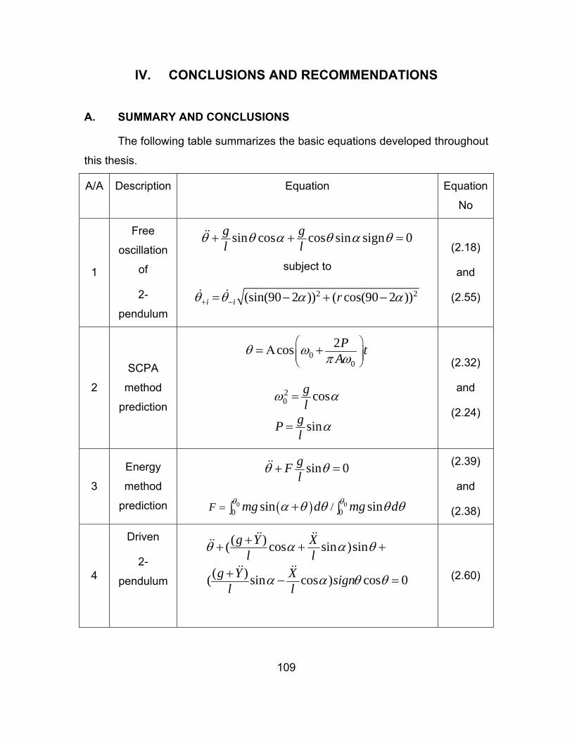
109
IV. CONCLUSIONS AND RECOMMENDATIONS
A. SUMMARY AND CONCLUSIONS
The following table summarizes the basic equations developed throughout
this thesis.
A/A Description Equation Equation
No
1
Free
oscillation
of
2-
pendulum
sin cos cos sin sign 0θ θ α θ α θ+ + =g gl l
subject to
2 2(sin(90 2 )) ( cos(90 2 ))θ θ α α+ −= − + −i i r
(2.18)
and
(2.55)
2
SCPA
method
prediction
00
2cosθ ωπ ω
⎛ ⎞⎜ ⎟⎜ ⎟⎝ ⎠
= Α + P tA
20 cos
sin
ω α
α
=
=
gl
gPl
(2.32)
and
(2.24)
3
Energy
method
prediction
sin 0θ θ+ =gFl
( )0 00 0/sin sinθ θα θ θ θ θ= +∫ ∫F mg d mg d
(2.39)
and
(2.38)
4
Driven
2-
pendulum
( )( cos sin )sin
( )( sin cos ) cos 0
θ α α θ
α α θ θ
++ + +
+ − =
g Y Xl l
g Y X signl l
(2.60)
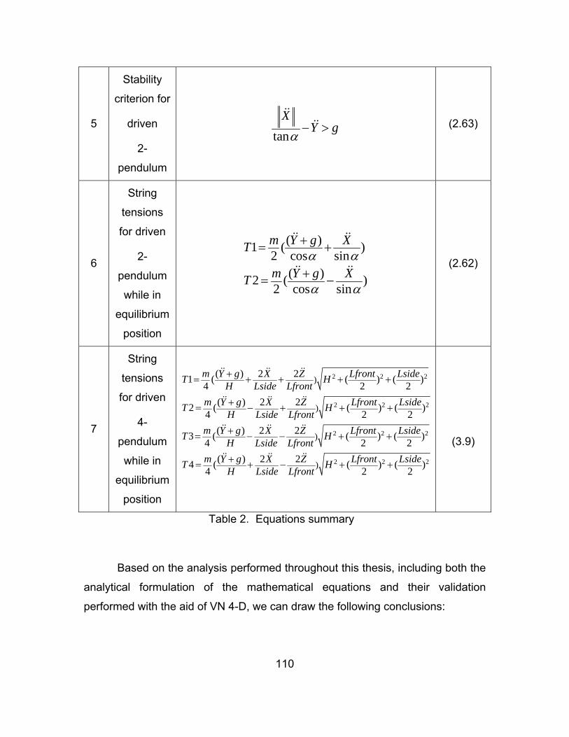
110
5
Stability
criterion for
driven
2-
pendulum
tanα− >
XY g (2.63)
6
String
tensions
for driven
2-
pendulum
while in
equilibrium
position
( )1 ( )2 cos sin
( )2 ( )2 cos sin
α α
α α
+= +
+= −
m Y g XT
m Y g XT (2.62)
7
String
tensions
for driven
4-
pendulum
while in
equilibrium
position
2 2 2
2 2 2
2 2 2
)
)
)
( ) 2 21 ( ( ) ( )4 2 2
( ) 2 22 ( ( ) ( )4 2 2
( ) 2 23 ( ( ) ( )4 2 2
( ) 24 (4
m Y g X Z Lfront LsideT HH Lside Lfront
m Y g X Z Lfront LsideT HH Lside Lfront
m Y g X Z Lfront LsideT HH Lside Lfront
m Y g XTH Lsid
+= + + + +
+= − + + +
+= − − + +
+= + 2 2 2)2 ( ) ( )2 2
Z Lfront LsideHe Lfront− + +
(3.9)
Table 2. Equations summary
Based on the analysis performed throughout this thesis, including both the
analytical formulation of the mathematical equations and their validation
performed with the aid of VN 4-D, we can draw the following conclusions:
111
• The 2-pendulum’s configuration of two strings per mass
introduces two distinct nonlinear oscillation characteristics. The first one results
from the discontinuity in its stiffness around the equilibrium position, i.e. an
instantaneous jump in the value of the restoring moment around zero. Four
different methods, were used to incorporate this discontinuity in analytical
equation formulation: Numerical solution with ode45, exact solution for a time
increment, SCPA method and Energy method.
• The second nonlinear oscillation characteristic is related to
the energy dissipation that takes place at the switch point. The dynamics that
govern this behavior are correlated to the dynamics of a standard collision of a
mass on a rigid wall, with specific velocity direction constraints before and after
the collision. The idealized model is based on an instantaneous impact and total
energy loss related to the mass’ velocity component parallel to the taught string’s
direction. This assumption is validated by the VN 4-D simulation.
• Another characteristic that was analyzed was the stability of
the 2-string pendulum in forced oscillation. This string configuration results in the
absence of oscillatory behavior if the mass is initially at the equilibrium position
and the driving horizontal and vertical accelerations do not exceed values
determined exclusively by the characteristic angle α. This observation allows the
rational design of support systems under given support motion characteristics.
• The general behavior of the driven 2-pendulum was
investigated including the case of induced jumps. Specific examples
demonstrated the highly non-nonlinear behavior of the 2-pendulum when
extreme acceleration values of the support cause the strings to go slack.
• Finally, the analysis of the 2-pendulum was extended on the
4-pendulum configuration, which is a more common support design in practice. A
typical optimization study was presented in order to visualize the practical design

112
advantages that such an analysis offers. It was shown that it is possible to
reduce both motions and cable tensions by appropriate selections of string
angles.
B. RECOMMENDATIONS
Further development of the analysis presented in this work could be in the
application of angular support motion, both for the case of forced oscillations of
the 2-pendulum and the trade off analysis. This work would provide a more
realistic representation of the support motion analogous to the motion of the ship.
Further extensions to this work by considering the effects of string elasticity are
also recommended.

113
APPENDIX: COMPUTER PROGRAMS
%Program_1.m %---------------------------------------------------------------------- %---------------------------------------------------------------------- %Computing the response of free 2-pendulum using three distinct methods: Numerical solution, SCPA method and Energy method %---------------------------------------------------------------------- %---------------------------------------------------------------------- clear all clc close all global a omega2 A omega P maxy1 Thetao t increased_restoring THETAo=pi/10 %initial angular displacement THETAo_dot=0 %initial angular velocity a=input('Give the characteristic angle a ');%2-pendulum's characteristic %angle g=9.81; %acceleration of gravity ll=1; %equivalent string length which equals to the
%simple pendulum string length or the %perpendicular distance of the mass from %the plane of suspension
l=ll/cos(a) %string length of complex pendulum omega2=g/l; %square of the natural frequency of the % standard pendulum omega2o=omega2*cos(a); %square of the pseudo natural frequency of the %2-pendulum tf=3; %final time %---------------------------------------------------------------------- %---------------------------------------------------------------------- %Numerical solution of the differential equation of motion %---------------------------------------------------------------------- %---------------------------------------------------------------------- options = odeset('RelTol',1e-6,'AbsTol',[1e-6 1e-6]); [t,x]=ode45('Ffull',[0:0.01:tf],[THETAo,THETAo_dot],options); [t,x(:,1)]; X1=x; figure (1) hold on title('\alpha=\pi/6') plot(t,x(:,1),'g')
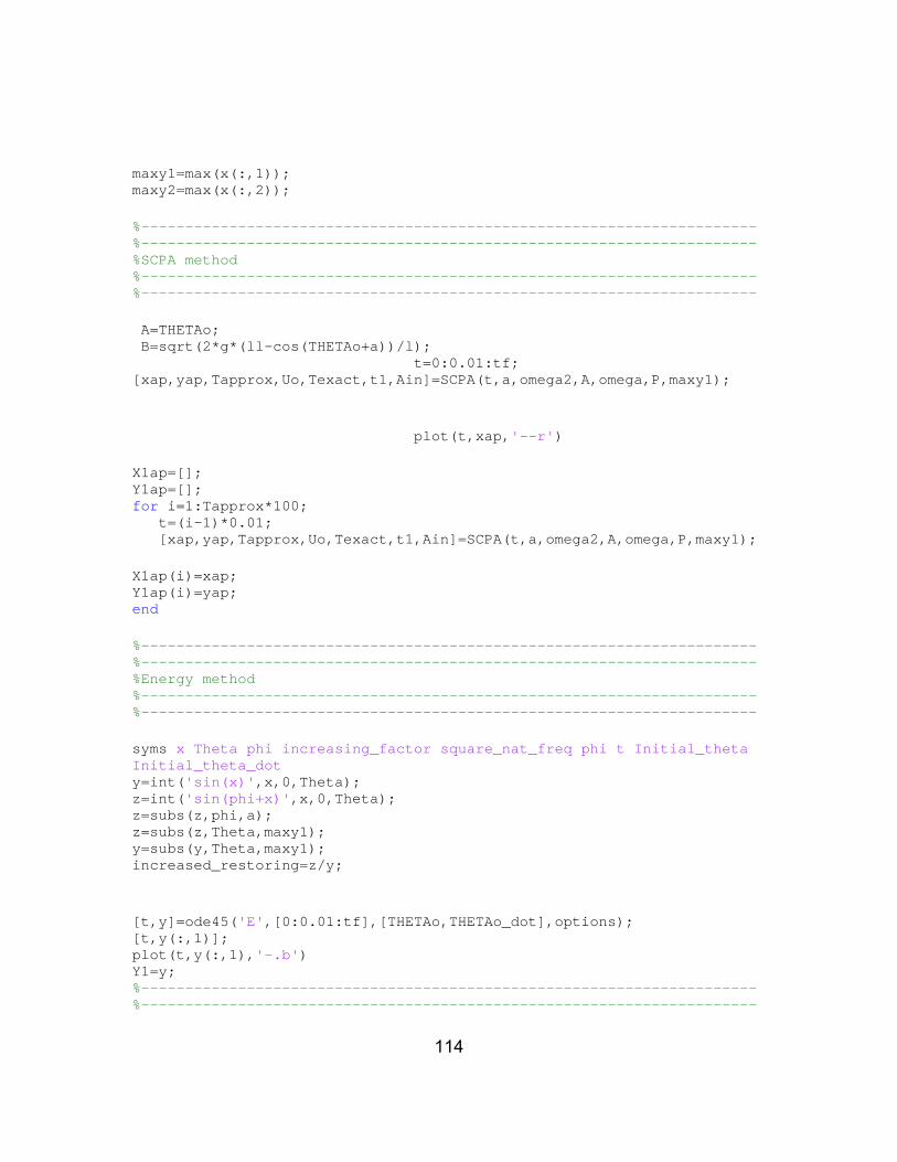
114
maxy1=max(x(:,1)); maxy2=max(x(:,2)); %---------------------------------------------------------------------- %---------------------------------------------------------------------- %SCPA method %---------------------------------------------------------------------- %---------------------------------------------------------------------- A=THETAo; B=sqrt(2*g*(ll-cos(THETAo+a))/l); t=0:0.01:tf; [xap,yap,Tapprox,Uo,Texact,t1,Ain]=SCPA(t,a,omega2,A,omega,P,maxy1); plot(t,xap,'--r') X1ap=[]; Y1ap=[]; for i=1:Tapprox*100; t=(i-1)*0.01; [xap,yap,Tapprox,Uo,Texact,t1,Ain]=SCPA(t,a,omega2,A,omega,P,maxy1); X1ap(i)=xap; Y1ap(i)=yap; end %---------------------------------------------------------------------- %---------------------------------------------------------------------- %Energy method %---------------------------------------------------------------------- %---------------------------------------------------------------------- syms x Theta phi increasing_factor square_nat_freq phi t Initial_theta Initial_theta_dot y=int('sin(x)',x,0,Theta); z=int('sin(phi+x)',x,0,Theta); z=subs(z,phi,a); z=subs(z,Theta,maxy1); y=subs(y,Theta,maxy1); increased_restoring=z/y; [t,y]=ode45('E',[0:0.01:tf],[THETAo,THETAo_dot],options); [t,y(:,1)]; plot(t,y(:,1),'-.b') Y1=y; %---------------------------------------------------------------------- %----------------------------------------------------------------------

115
t=0:0.01:tf; xlabel('t (sec)') ylabel('\theta (rad)') grid on box on legend('ODE45 ','SCPA method','Energy method') axis([0 tf -1.25*maxy1 0.6]) hold off Tapprox1=Tapprox; % Approximate Period of the Slowly Changing method Texact1=Texact; %Period from the analytical solution calculating % for the time period when the sign of theta is %constant figure (2) title('\alpha=\pi/6') hold on plot(X1(1:Texact1*100,1)./THETAo,X1(1:Texact1*100,2)./sqrt(omega2o),'g',X1ap./THETAo,Y1ap./sqrt(omega2o),'--r', Y1(1:Tapprox1*100,1)./THETAo,Y1(1:Tapprox1*100,2)./sqrt(omega2o),'-.b') grid on box on xlabel('\theta/\thetao');ylabel('\theta''/\omega\o') legend('ODE45 ','SCPA method','Energy method') axis([-1.5 1.5 -1 1]) hold off
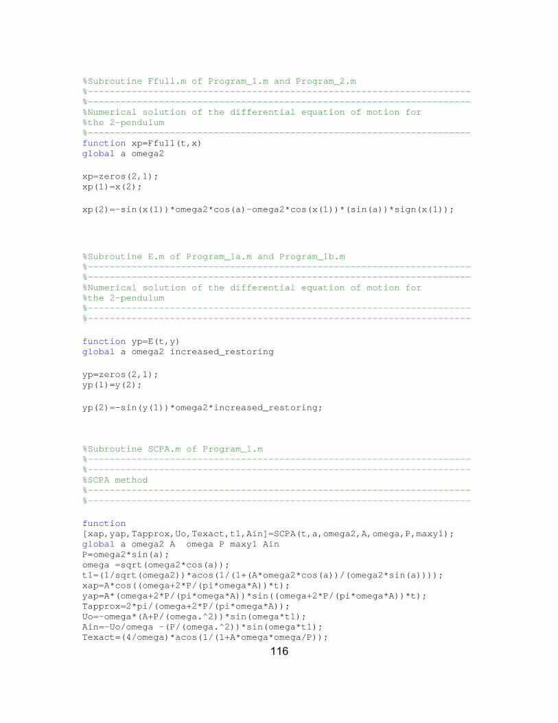
116
%Subroutine Ffull.m of Program_1.m and Program_2.m %---------------------------------------------------------------------- %---------------------------------------------------------------------- %Numerical solution of the differential equation of motion for %the 2-pendulum %---------------------------------------------------------------------- function xp=Ffull(t,x) global a omega2 xp=zeros(2,1); xp(1)=x(2); xp(2)=-sin(x(1))*omega2*cos(a)-omega2*cos(x(1))*(sin(a))*sign(x(1));
%Subroutine E.m of Program_1a.m and Program_1b.m %---------------------------------------------------------------------- %---------------------------------------------------------------------- %Numerical solution of the differential equation of motion for %the 2-pendulum %---------------------------------------------------------------------- %---------------------------------------------------------------------- function yp=E(t,y) global a omega2 increased_restoring yp=zeros(2,1); yp(1)=y(2); yp(2)=-sin(y(1))*omega2*increased_restoring; %Subroutine SCPA.m of Program_1.m %---------------------------------------------------------------------- %---------------------------------------------------------------------- %SCPA method %---------------------------------------------------------------------- %---------------------------------------------------------------------- function [xap,yap,Tapprox,Uo,Texact,t1,Ain]=SCPA(t,a,omega2,A,omega,P,maxy1); global a omega2 A omega P maxy1 Ain P=omega2*sin(a); omega =sqrt(omega2*cos(a)); t1=(1/sqrt(omega2))*acos(1/(1+(A*omega2*cos(a))/(omega2*sin(a)))); xap=A*cos((omega+2*P/(pi*omega*A))*t); yap=A*(omega+2*P/(pi*omega*A))*sin((omega+2*P/(pi*omega*A))*t); Tapprox=2*pi/(omega+2*P/(pi*omega*A)); Uo=-omega*(A+P/(omega.^2))*sin(omega*t1); Ain=-Uo/omega -(P/(omega.^2))*sin(omega*t1); Texact=(4/omega)*acos(1/(1+A*omega*omega/P));
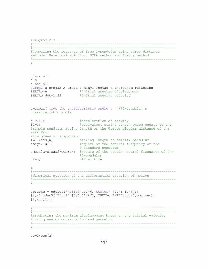
117
%Program_2.m %---------------------------------------------------------------------- %---------------------------------------------------------------------- %Computing the response of free 2-pendulum using three distinct methods: Numerical solution, SCPA method and Energy method %---------------------------------------------------------------------- %---------------------------------------------------------------------- clear all clc close all global a omega2 A omega P maxy1 Thetao t increased_restoring THETAo=0 %initial angular displacement THETAo_dot=1.22 %initial angular velocity a=input('Give the characteristic angle a ');%2-pendulum's characteristic angle g=9.81; %acceleration of gravity ll=1; %equivalent string length which equals to the %simple pendulum string length or the %perpendicular distance of the mass from %the plane of suspension l=ll/cos(a) %string length of complex pendulum omega2=g/l; %square of the natural frequency of the % standard pendulum omega2o=omega2*cos(a); %square of the pseudo natural frequency of the %2-pendulum tf=3; %final time %---------------------------------------------------------------------- %---------------------------------------------------------------------- %Numerical solution of the differential equation of motion %---------------------------------------------------------------------- %---------------------------------------------------------------------- options = odeset('RelTol',1e-6,'AbsTol',[1e-6 1e-6]); [t,x]=ode45('Ffull',[0:0.01:tf],[THETAo,THETAo_dot],options); [t,x(:,1)]; %----------------------------------------------------------------------%---------------------------------------------------------------------- %Predicting the maximum displacement based on the initial velocity % using energy conservation and geometry %---------------------------------------------------------------------- %---------------------------------------------------------------------- so=l*cos(a);
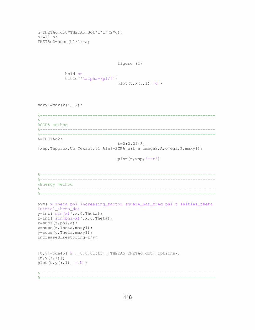
118
h=THETAo_dot*THETAo_dot*l*l/(2*g); h1=ll-h; THETAo2=acos(h1/l)-a; figure (1) hold on title('\alpha=\pi/6') plot(t,x(:,1),'g') maxy1=max(x(:,1)); %---------------------------------------------------------------------- %---------------------------------------------------------------------- %SCPA method %---------------------------------------------------------------------- %---------------------------------------------------------------------- A=THETAo2; t=0:0.01:3; [xap,Tapprox,Uo,Texact,t1,Ain]=SCPA_u(t,a,omega2,A,omega,P,maxy1); plot(t,xap,'--r') %---------------------------------------------------------------------- %---------------------------------------------------------------------- %Energy method %---------------------------------------------------------------------- %---------------------------------------------------------------------- syms x Theta phi increasing_factor square_nat_freq phi t Initial_theta Initial_theta_dot y=int('sin(x)',x,0,Theta); z=int('sin(phi+x)',x,0,Theta); z=subs(z,phi,a); z=subs(z,Theta,maxy1); y=subs(y,Theta,maxy1); increased_restoring=z/y; [t,y]=ode45('E',[0:0.01:tf],[THETAo,THETAo_dot],options); [t,y(:,1)]; plot(t,y(:,1),'-.b') %---------------------------------------------------------------------- %----------------------------------------------------------------------
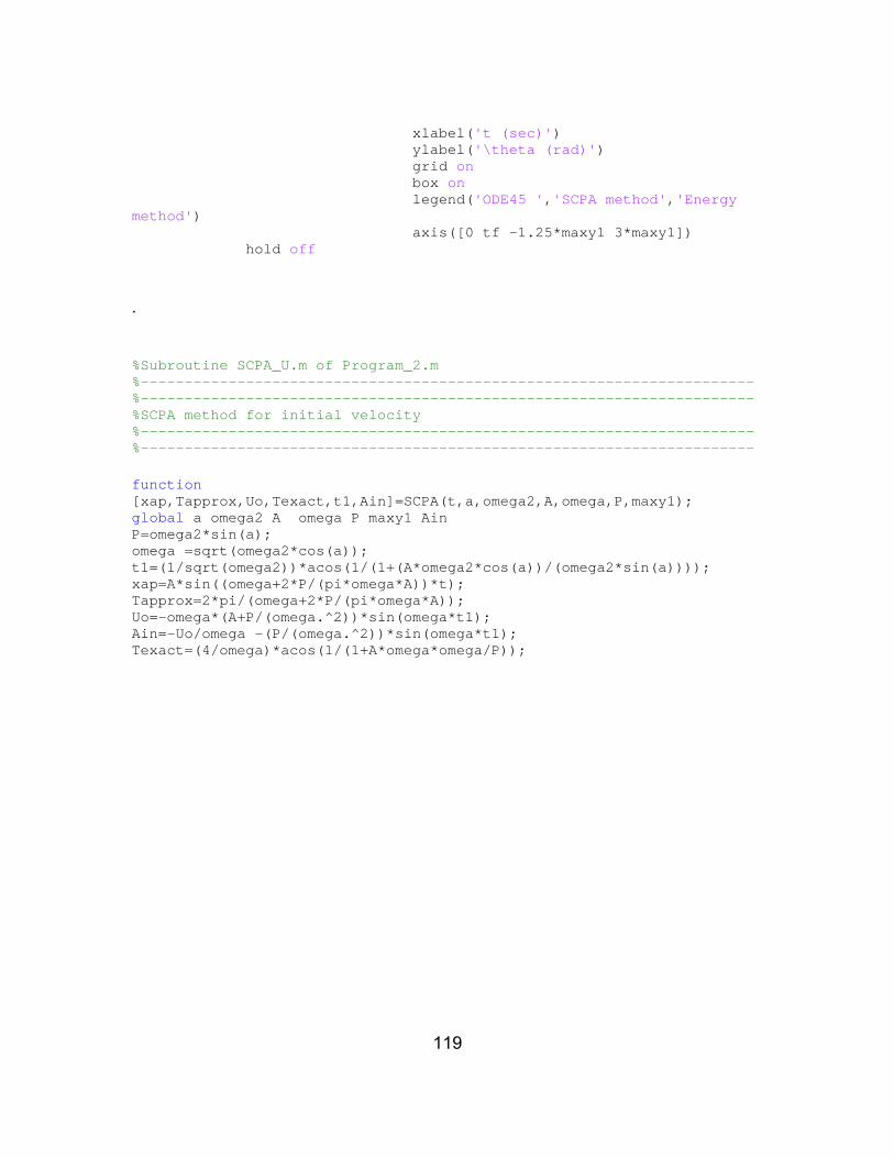
119
xlabel('t (sec)') ylabel('\theta (rad)') grid on box on legend('ODE45 ','SCPA method','Energy method') axis([0 tf -1.25*maxy1 3*maxy1]) hold off
. %Subroutine SCPA_U.m of Program_2.m %---------------------------------------------------------------------- %---------------------------------------------------------------------- %SCPA method for initial velocity %---------------------------------------------------------------------- %---------------------------------------------------------------------- function [xap,Tapprox,Uo,Texact,t1,Ain]=SCPA(t,a,omega2,A,omega,P,maxy1); global a omega2 A omega P maxy1 Ain P=omega2*sin(a); omega =sqrt(omega2*cos(a)); t1=(1/sqrt(omega2))*acos(1/(1+(A*omega2*cos(a))/(omega2*sin(a)))); xap=A*sin((omega+2*P/(pi*omega*A))*t); Tapprox=2*pi/(omega+2*P/(pi*omega*A)); Uo=-omega*(A+P/(omega.^2))*sin(omega*t1); Ain=-Uo/omega -(P/(omega.^2))*sin(omega*t1); Texact=(4/omega)*acos(1/(1+A*omega*omega/P));

120
%Program_3.m %---------------------------------------------------------------------- %---------------------------------------------------------------------- %Computing the response of the driven 2-pendulum for a given and % specific set of support motion %---------------------------------------------------------------------- %---------------------------------------------------------------------- %---------------------------------------------------------------------- %%%%%%%%%%%%%%%%%%%%%%%%%%%%%%ATTENTION%%%%%%%%%%%%%%%%%%%%%%%%%%%%%%%% %this m-file is valid only when the appropriate and specific data_1.m %and data_2.m data files exist in the same folder since those files % contain both the support motion info and the corresponding results % from Nastran for comparison and validation purposes %---------------------------------------------------------------------- clc clear all format long fprintf('make sure that you have copied the data provided by Nastran') datainput=input('if you already have press 1 ') if datainput==1 fprintf('good to go') else break end %call the data file dat=input('choose the data file, 1 for latteral and vertical motion, 2 for latteral motion') if dat==1 data_1 else data_2 end %---------------------------------------------------------------------- %---------------------------------------------------------------------- %response before the stability is broken %---------------------------------------------------------------------- %---------------------------------------------------------------------- ti=0; %initial time condition tf=length(data(:,2))/1000-0.001;%final time condition dt=0.001; %time step

121
nt=fix((tf-ti)/dt) %number of time steps a=pi/18; %pendulation characteristic angle g=9.81; %acceleration of gravity ll=1; %equivalent string length which equals to the %simple pendulum string length or the %perpendicular distance of the mass from the % plane of suspension l=ll/cos(a); %string length of complex pendulum omega2=g/l; %square of the natural frequency of the simple %pendulum omega2o=omega2*cos(a); %square of the pseudo natural frequency of the %2-pendulum r=0; %restitution coefficient m=1; %mass %---------------------------------------------------------------------- %initializing the acceleration, velocity and displacement vectors %---------------------------------------------------------------------- acc=zeros(1,nt+1); %mass angular acceleration vel=zeros(1,nt+1); %mass angular velocity disp=zeros(1,nt+1); %mass angular displacement force=zeros(1,nt+1); %pseudo-restoring force on mass Zabs=zeros(1,nt+1); %absolute horizontal position of mass Yabs=zeros(1,nt+1); %absolute vertical position of mass Z=zeros(1,nt+1); %global horizontal position of mass Y=zeros(1,nt+1); %global vertical position of mass Zs=zeros(1,nt+1); %global horizontal position of support midpoint Ys=zeros(1,nt+1); %global vertical position of support midpoint acc_rest=zeros(1,nt+1); %pseudo-acceleration corresponding to the case %that the mass doesn't break stability Zsddot=zeros(1,nt+1); %global horizontal acceleration of support %midpoint Ysddot=zeros(1,nt+1); %global vertical acceleration of support %midpoint Zsdot=zeros(1,nt+1); %global horizontal velocity of support midpoint Ysdot=zeros(1,nt+1); %global vertical velocity of support midpoint Zsdot(1,1)=0; Ysdot(1,1)=0; Zsddot(1,1)=0; Ysddot(1,1)=0; Vzj=zeros(1,nt+1); %linear horizontal velocity of mass during jump Vyj=zeros(1,nt+1); %linear vertical velocity of mass during jump %---------------------------------------------------------------------- %applying the data input in the support midpoint motion %---------------------------------------------------------------------- if dat==1 Zs=data(:,2)'./1000; Ys=data(:,3)'./1000; else Zs=data(:,2)'./1000; Ys=zeros(1,nt+1); end
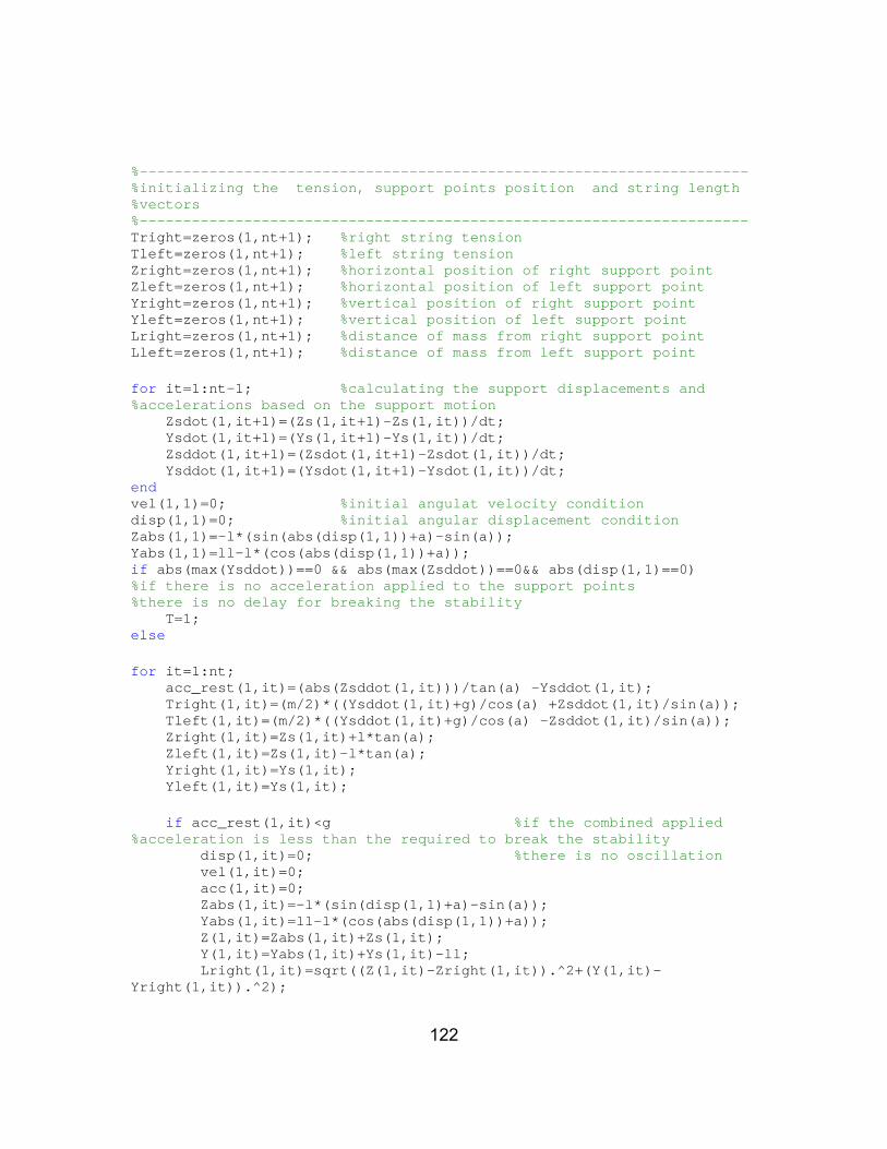
122
%---------------------------------------------------------------------- %initializing the tension, support points position and string length %vectors %---------------------------------------------------------------------- Tright=zeros(1,nt+1); %right string tension Tleft=zeros(1,nt+1); %left string tension Zright=zeros(1,nt+1); %horizontal position of right support point Zleft=zeros(1,nt+1); %horizontal position of left support point Yright=zeros(1,nt+1); %vertical position of right support point Yleft=zeros(1,nt+1); %vertical position of left support point Lright=zeros(1,nt+1); %distance of mass from right support point Lleft=zeros(1,nt+1); %distance of mass from left support point for it=1:nt-1; %calculating the support displacements and %accelerations based on the support motion Zsdot(1,it+1)=(Zs(1,it+1)-Zs(1,it))/dt; Ysdot(1,it+1)=(Ys(1,it+1)-Ys(1,it))/dt; Zsddot(1,it+1)=(Zsdot(1,it+1)-Zsdot(1,it))/dt; Ysddot(1,it+1)=(Ysdot(1,it+1)-Ysdot(1,it))/dt; end vel(1,1)=0; %initial angulat velocity condition disp(1,1)=0; %initial angular displacement condition Zabs(1,1)=-l*(sin(abs(disp(1,1))+a)-sin(a)); Yabs(1,1)=ll-l*(cos(abs(disp(1,1))+a)); if abs(max(Ysddot))==0 && abs(max(Zsddot))==0&& abs(disp(1,1)==0) %if there is no acceleration applied to the support points %there is no delay for breaking the stability T=1; else for it=1:nt; acc_rest(1,it)=(abs(Zsddot(1,it)))/tan(a) -Ysddot(1,it); Tright(1,it)=(m/2)*((Ysddot(1,it)+g)/cos(a) +Zsddot(1,it)/sin(a)); Tleft(1,it)=(m/2)*((Ysddot(1,it)+g)/cos(a) -Zsddot(1,it)/sin(a)); Zright(1,it)=Zs(1,it)+l*tan(a); Zleft(1,it)=Zs(1,it)-l*tan(a); Yright(1,it)=Ys(1,it); Yleft(1,it)=Ys(1,it); if acc_rest(1,it)<g %if the combined applied %acceleration is less than the required to break the stability disp(1,it)=0; %there is no oscillation vel(1,it)=0; acc(1,it)=0; Zabs(1,it)=-l*(sin(disp(1,1)+a)-sin(a)); Yabs(1,it)=ll-l*(cos(abs(disp(1,1))+a)); Z(1,it)=Zabs(1,it)+Zs(1,it); Y(1,it)=Yabs(1,it)+Ys(1,it)-ll; Lright(1,it)=sqrt((Z(1,it)-Zright(1,it)).^2+(Y(1,it)-Yright(1,it)).^2);
123
Lleft(1,it)=sqrt((Z(1,it)-Zleft(1,it)).^2+(Y(1,it)-Yleft(1,it)).^2); else T=it; Zabs(1,it)=-l*(sin(disp(1,1)+a)-sin(a)); Yabs(1,it)=ll-l*(cos(abs(disp(1,1))+a)); Z(1,it)=Zabs(1,it)+Zs(1,it); Y(1,it)=Yabs(1,it)+Ys(1,it)-ll; Lright(1,it)=sqrt((Z(1,it)-Zright(1,it)).^2+(Y(1,it)-Yright(1,it)).^2); Lleft(1,it)=sqrt((Z(1,it)-Zleft(1,it)).^2+(Y(1,it)-Yleft(1,it)).^2); Vz1=Zsdot(1,T); Vy1=Ysdot(1,T); ACC=Zsddot(1,T); break end end end %---------------------------------------------------------------------- %---------------------------------------------------------------------- %Step after the stability is broken %---------------------------------------------------------------------- %---------------------------------------------------------------------- for it=T:nt; %loop1 - initiating calculations after %stability is brocken if (Tright(1,it)>0 || Tleft(1,it)>0)%condition1 - oscillations take %place only if at least one of the tensions has a non-zero value force(1,it)=-(omega2+Ysddot(1,it)/l)*(sin(a))*cos(disp(1,it))*sign(disp(1,it)); acc(1,it)=force(1,it)-(omega2+Ysddot(1,it)/l)*sin(disp(1,it))*cos(a)+(Zsddot(1,it))*((cos(abs(disp(1,it))+a)))/l; vel(1,it+1)=vel(1,it)+acc(1,it)*dt; disp(1,it+1)=disp(1,it)+vel(1,it+1)*dt; if disp(1,it+1)*disp(1,it)>=0 %condition2 - calculations %while the mass oscillates without changing strings disp(1,it+1)=disp(1,it)+vel(1,it+1)*dt; Zabs(1,it+1)=-sign((disp(1,it+1)))*l*(sin(abs(disp(1,it+1))+a)-sin(a)); Yabs(1,it+1)=ll-l*(cos(abs(disp(1,it+1))+a)); Z(1,it+1)=Zabs(1,it+1)+Zs(1,it+1); Y(1,it+1)=Yabs(1,it+1)+Ys(1,it+1)-ll; Zright(1,it)=Zs(1,it)+l*tan(a); Zleft(1,it)=Zs(1,it)-l*tan(a); Yright(1,it)=Ys(1,it); Yleft(1,it)=Ys(1,it);
124
Lright(1,it)=sqrt((Z(1,it)-Zright(1,it)).^2+(Y(1,it)-Yright(1,it)).^2); Lleft(1,it)=sqrt((Z(1,it)-Zleft(1,it)).^2+(Y(1,it)-Yleft(1,it)).^2); else %condition2 - the mass reached %a string switch point T1=it; V=vel(1,T1); Vaft=sign(V)*sqrt((V*sin(pi/2 -2*a)).^2+(r*V*cos(pi/2 -2*a)).^2); vel(1,T1+1)=Vaft; disp(1,T1+1)=disp(1,it)+vel(1,T1+1)*dt; Zabs(1,it+1)=-sign((disp(1,it+1)))*l*(sin(abs(disp(1,it+1))+a)-sin(a)); Yabs(1,it+1)=ll-l*(cos(abs(disp(1,it+1))+a)); Z(1,it+1)=Zabs(1,it+1)+Zs(1,it+1); Y(1,it+1)=Yabs(1,it+1)+Ys(1,it+1)-ll; Zright(1,it)=Zs(1,it)+l*tan(a); Zleft(1,it)=Zs(1,it)-l*tan(a); Yright(1,it)=Ys(1,it); Yleft(1,it)=Ys(1,it); Lright(1,it)=sqrt((Z(1,it)-Zright(1,it)).^2+(Y(1,it)-Yright(1,it)).^2); Lleft(1,it)=sqrt((Z(1,it)-Zleft(1,it)).^2+(Y(1,it)-Yleft(1,it)).^2); end %condition2 if disp(1,it+1)>0 %condition3 - calculating %the strings tension depending on which one of the strings is taught Tright(1,it+1)=m*(vel(1,it+1)*vel(1,it+1)*l+Zsddot(1,it+1)*sin(abs(disp(1,it+1))+a)+(g+Ysddot(1,it+1))*cos(abs(disp(1,it+1))+a)); Tleft(1,it+1)=0; if Tright(1,it+1)>0 Tright(1,it+1)=Tright(1,it+1); else Tright(1,it+1)=0; end else %condition3 Tleft(1,it+1)=m*(vel(1,it+1)*vel(1,it+1)*l-Zsddot(1,it+1)*sin(abs(disp(1,it+1))+a)+(g+Ysddot(1,it+1))*cos(abs(disp(1,it+1))+a)); Tright(1,it+1)=0; if Tleft(1,it+1)>0 Tleft(1,it+1)=Tleft(1,it+1); else Tleft(1,it+1)=0; end end %condition3 else %condition1 - the first %jump starts
125
T2=it V=vel(1,T2); disp(1,T2+1)=disp(1,T2)+vel(1,T2)*dt; Zabs(1,it)=-sign((disp(1,it)))*l*(sin(abs(disp(1,it))+a)-sin(a)); Yabs(1,it+1)=ll-l*(cos(abs(disp(1,it))+a)); Z(1,it)=Zabs(1,it)+Zs(1,it); Y(1,it)=Yabs(1,it)+Ys(1,it)-ll; Zright(1,it)=Zs(1,it)+l*tan(a); Zleft(1,it)=Zs(1,it)-l*tan(a); Yright(1,it)=Ys(1,it); Yleft(1,it)=Ys(1,it); Lright(1,it)=sqrt((Z(1,it)-Zright(1,it)).^2+(Y(1,it)-Yright(1,it)).^2); Lleft(1,it)=sqrt((Z(1,it)-Zleft(1,it)).^2+(Y(1,it)-Yleft(1,it)).^2); if disp(1,T2)>0 %condition4 - calculating %the linear velocity of the mass at the moment where the jump initiates Vmagn=abs(l*vel(1,T2)); Vz2=-sign(V)*Vmagn*cos((disp(1,T2)+a))+Zsdot(1,T2-1); Vy2=sign(V)*Vmagn*sin((disp(1,T2)+a))+Ysdot(1,T2-1); break else %condition4 Vmagn=l*abs(vel(1,T2)); Vz2=-sign(V)*Vmagn*cos((abs(disp(1,T2))+a))+Zsdot(1,T2-1); Vy2=-sign(V)*Vmagn*sin((abs(disp(1,T2))+a))+Ysdot(1,T2-1); break end %condition4 end %condition1 end %loop1 %correcting the computation rounding errors LLright=Lright(1,T2)-0.004; LLleft=Lleft(1,T2)-0.004; Lright(1,T2)=Lright(1,T2)-0.004; Lleft(1,T2)=Lleft(1,T2)-0.004; while it<nt jump afterjump end time =data(:,1); if dat==1
126
figure (4) plot(time,disp,time,data(:,4),'--r') xlabel('t (sec)');ylabel('\theta(rad)'); axis([0 tf -pi/2 pi/2]) grid on figure (5) subplot(2,1,1);plot(time,Zabs,time,data(:,10)./1000,'--r' ) xlabel('t (sec)');ylabel('absolute horizontal position (m)'); grid on axis([0 tf -1 1]) subplot(2,1,2);plot(time,Yabs,time,data(:,9)./1000+ll ,'--r' ) xlabel('t (sec)');ylabel('absolute vertical position (m)'); grid on axis([0 tf -1 1]) figure (6) subplot(2,1,1);plot(time,Z,time,data(:,8)./1000 ,'--r' ) xlabel('t (sec)');ylabel('total horizontal position (m)'); grid on axis([0 tf -1 3]) subplot(2,1,2);plot(time,Y,time,data(:,7)./1000 ,'--r' ) xlabel('t (sec)');ylabel('total vertical position (m)'); grid on axis([0 tf -1 1]) else figure (4) plot(time,disp,time,data(:,3),'--r') xlabel('t (sec)');ylabel('\theta(rad)'); axis([0 tf -pi/2 pi/2]) grid on figure (5) subplot(2,1,1);plot(time,Zabs,time,data(:,4)./1000-Zs','--r' ) xlabel('t (sec)');ylabel('absolute horizontal position (m)'); grid on axis([0 tf -1 1]) subplot(2,1,2);plot(time,Yabs,time,data(:,5)./1000+ll-Ys' ,'--r' ) xlabel('t (sec)');ylabel('absolute vertical position (m)'); grid on axis([0 tf -1 1]) figure (6) subplot(2,1,1);plot(time,Z,time,data(:,4)./1000 ,'--r' ) xlabel('t (sec)');ylabel('total horizontal position (m)'); grid on axis([0 tf -1 5]) subplot(2,1,2);plot(time,Y,time,data(:,5)./1000 ,'--r' ) xlabel('t (sec)');ylabel('total vertical position (m)'); grid on axis([0 tf -1 0]) end figure (7) subplot(2,1,1);plot(time,Lright ) xlabel('t (sec)');ylabel('absolute horizontal position (m)'); grid on
127
axis([0 tf 0 2]) subplot(2,1,2);plot(time,Lleft ) xlabel('t (sec)');ylabel('absolute vertical position (m)'); grid on axis([0 tf 0 2]) figure (8) subplot(2,1,1);plot(time,Zs ) xlabel('t (sec)');ylabel(' horizontal support position (m)'); grid on axis([0 tf 0 5]) subplot(2,1,2);plot(time,Ys ) xlabel('t (sec)');ylabel('vertical support position (m)'); grid on axis([0 tf -1 2]) figure (10) plot(time,Tright, time, Tleft) xlabel('t (sec)'); ylabel('tension (N)') legend('right string','left string') axis tight %jump.m subroutine - part of the Program_3.m code %---------------------------------------------------------------------- %---------------------------------------------------------------------- %Computing the response of the driven 2-pendulum when a jump is initiated %---------------------------------------------------------------------- %---------------------------------------------------------------------- %---------------------------------------------------------------------- %---------------------------------------------------------------------- %collecting data from the main file %---------------------------------------------------------------------- %---------------------------------------------------------------------- Lright(1,T2)=LLright; Lleft(1,T2)=LLleft; Vyj(1,T2)=Vy2; Vzj(1,T2)=Vz2;
128
for it=T2+1:nt; %loop1 - initiating %calculations if (Lleft(1,it-1)>l || Lright(1,it-1)>l) %condition1 - if the %length of at least one of the strings is equal to l, the the jump is %terminated T3=it; Zright(1,it)=Zs(1,it)+l*tan(a); Zleft(1,it)=Zs(1,it)-l*tan(a); Yright(1,it)=Ys(1,it); Yleft(1,it)=Ys(1,it); Vzj(1,it)=Vz2; Vyj(1,it)=Vyj(1,it-1)-(g)*dt; Z(1,it)=Z(1,it-1)+Vz2*dt; Y(1,it)=Y(1,it-1)+Vyj(1,it)*dt; Zabs(1,it)=Z(1,it)-Zs(1,it); Yabs(1,it)=ll+Y(1,it)-Ys(1,it); vel(1,it)=0; disp(1,it)=0; Vzj1=Vzj(1,it); Vyj1=Vyj(1,it); Lright(1,it)=sqrt((Z(1,it)-Zright(1,it)).^2+(Y(1,it)-Yright(1,it)).^2)-0.004; Lleft(1,it)=sqrt((Z(1,it)-Zleft(1,it)).^2+(Y(1,it)-Yleft(1,it)).^2)-0.004; Vmagnj=sqrt(Vzj1*Vzj1+Vyj1+Vyj1); break else Vzj(1,it)=Vz2; %condition1 - the mass %follows a projectile path Vyj(1,it)=Vyj(1,it-1)-(g)*dt; %during the jump Z(1,it)=Z(1,it-1)+Vz2*dt; Y(1,it)=Y(1,it-1)+Vyj(1,it)*dt; Zabs(1,it)=Z(1,it)-Zs(1,it); Yabs(1,it)=ll+Y(1,it)-Ys(1,it); Zright(1,it)=Zs(1,it)+l*tan(a); Zleft(1,it)=Zs(1,it)-l*tan(a); Yright(1,it)=Ys(1,it); Yleft(1,it)=Ys(1,it); Lright(1,it)=sqrt((Z(1,it)-Zright(1,it)).^2+(Y(1,it)-Yright(1,it)).^2)-0.004; Lleft(1,it)=sqrt((Z(1,it)-Zleft(1,it)).^2+(Y(1,it)-Yleft(1,it)).^2)-0.004; vel(1,it)=0; disp(1,it)=0; end %condition1 end %loop1 if Lright(1,T3)>Lleft(1,T3) %condition2 - calculating the angular displacement
129
phi=atan((Zright(1,T3)-Z(1,T3))/(Yright(1,T3)-Y(1,T3))); %and %the velocity of the mass after the alpha=atan(Vyj1/Vzj1); %jump %is terminated depending on which string is taught vel(1,T3)=(1/l)*(-Vzj1*cos(phi)+Vyj1*sin(phi)); disp(1,T3)=phi-a; Tright(1,T3)=m*(vel(1,T3)*vel(1,T3)*l+Zsddot(1,T3)*sin(abs(disp(1,T3))+a)+(g+Ysddot(1,T3))*cos(abs(disp(1,T3))+a)); Tleft(1,T3)=0; if Tright(1,it+1)>0 %condition3 - ensuring %that the string doesn't support compressive loads Tright(1,it+1)=Tright(1,it+1); else Tright(1,it+1)=0; end else %condition2 phi=atan((Z(1,T3)-Zleft(1,T3))/(Yleft(1,T3)-Y(1,T3))); phit=-phi; alpha=atan(Vzj1/Vyj1); alpha*180/pi; vel(1,T3)=(1/l)*(-Vzj1*cos(phi)-Vyj1*sin(phi)); disp(1,T3)=-(phi-a); Tleft(1,T3)=m*(vel(1,T3)*vel(1,T3)*l+Zsddot(1,T3)*sin(abs(disp(1,T3))+a)+(g+Ysddot(1,T3))*cos(abs(disp(1,T3))+a)); Tright(1,T3)=0; if Tleft(1,it+1)>0 %condition3 Tleft(1,it+1)=Tleft(1,it+1); else Tleft(1,it+1)=0; end end %condition2
130
%afterjump.m subroutine - part of the Program_3.m code %---------------------------------------------------------------------- %---------------------------------------------------------------------- %Computing the response of the driven 2-pendulum after a jump is %terminated %---------------------------------------------------------------------- %---------------------------------------------------------------------- for it=T3:nt; %loop1 - initiating calculations after stability is %broken if (Tright(1,it)>0 || Tleft(1,it)>0) %condition1 - oscillations take %place only if at least one of the tensions has a non-zero value force(1,it)=-(omega2+Ysddot(1,it)/l)*(sin(a))*cos(disp(1,it))*sign(disp(1,it)); acc(1,it)=force(1,it)-(omega2+Ysddot(1,it)/l)*sin(disp(1,it))*cos(a)+(Zsddot(1,it))*((cos(abs(disp(1,it))+a)))/l; vel(1,it+1)=vel(1,it)+acc(1,it)*dt; disp(1,it+1)=disp(1,it)+vel(1,it+1)*dt; if disp(1,it+1)*disp(1,it)>=0 %condition2 - calculations %while the mass oscillates without changing strings disp(1,it+1)=disp(1,it)+vel(1,it+1)*dt; Zabs(1,it+1)=-sign((disp(1,it+1)))*l*(sin(abs(disp(1,it+1))+a)-sin(a)); Yabs(1,it+1)=ll-l*(cos(abs(disp(1,it+1))+a)); Z(1,it+1)=Zabs(1,it+1)+Zs(1,it+1); Y(1,it+1)=Yabs(1,it+1)+Ys(1,it+1)-ll; Zright(1,it)=Zs(1,it)+l*tan(a); Zleft(1,it)=Zs(1,it)-l*tan(a); Yright(1,it)=Ys(1,it); Yleft(1,it)=Ys(1,it); Lright(1,it)=sqrt((Z(1,it)-Zright(1,it)).^2+(Y(1,it)-Yright(1,it)).^2); Lleft(1,it)=sqrt((Z(1,it)-Zleft(1,it)).^2+(Y(1,it)-Yleft(1,it)).^2); else %condition2 - the mass reached %a string switch point T2=it; V=vel(1,T2); Vaft=sign(V)*sqrt((V*sin(pi/2 -2*a)).^2+(r*V*cos(pi/2 -2*a)).^2); vel(1,T2+1)=Vaft; disp(1,T2+1)=disp(1,T2)+vel(1,T2+1)*dt; Zabs(1,it+1)=-sign((disp(1,it+1)))*l*(sin(abs(disp(1,it+1))+a)-sin(a));
131
Yabs(1,it+1)=ll-l*(cos(abs(disp(1,it+1))+a)); Z(1,it+1)=Zabs(1,it+1)+Zs(1,it+1); Y(1,it+1)=Yabs(1,it+1)+Ys(1,it+1)-ll; Zright(1,it)=Zs(1,it)+l*tan(a); Zleft(1,it)=Zs(1,it)-l*tan(a); Yright(1,it)=Ys(1,it); Yleft(1,it)=Ys(1,it); Lright(1,it)=sqrt((Z(1,it)-Zright(1,it)).^2+(Y(1,it)-Yright(1,it)).^2); Lleft(1,it)=sqrt((Z(1,it)-Zleft(1,it)).^2+(Y(1,it)-Yleft(1,it)).^2); end %condition2 if disp(1,it+1)>0 %condition3 - calculating the strings tension depending on which one of the strings is taught Tright(1,it+1)=m*(vel(1,it+1)*vel(1,it+1)*l+Zsddot(1,it+1)*sin(abs(disp(1,it+1))+a)+(g+Ysddot(1,it+1))*cos(abs(disp(1,it+1))+a)); Tleft(1,it+1)=0; if Tright(1,it+1)>0 %condition4 - ensuring that %the string doesn't support compressive loads Tright(1,it+1)=Tright(1,it+1); else Tright(1,it+1)=0; end else %condition3 Tleft(1,it+1)=m*(vel(1,it+1)*vel(1,it+1)*l-Zsddot(1,it+1)*sin(abs(disp(1,it+1))+a)+(g+Ysddot(1,it+1))*cos(abs(disp(1,it+1))+a)); Tright(1,it+1)=0; if Tleft(1,it+1)>0 %condition4 - ensuring that %the string doesn't support compressive loads Tleft(1,it+1)=Tleft(1,it+1); else Tleft(1,it+1)=0; end end %condition3 else %condition1 T2=it V=vel(1,T2); disp(1,T2+1)=disp(1,it)+vel(1,T2)*dt; Zabs(1,it)=-sign((disp(1,it)))*l*(sin(abs(disp(1,it))+a)-sin(a)); Yabs(1,it+1)=ll-l*(cos(abs(disp(1,it))+a)); Z(1,it)=Zabs(1,it)+Zs(1,it);
132
Y(1,it)=Yabs(1,it)+Ys(1,it)-ll; Zright(1,it)=Zs(1,it)+l*tan(a); Zleft(1,it)=Zs(1,it)-l*tan(a); Yright(1,it)=Ys(1,it); Yleft(1,it)=Ys(1,it); Lright(1,it)=sqrt((Z(1,it)-Zright(1,it)).^2+(Y(1,it)-Yright(1,it)).^2); Lleft(1,it)=sqrt((Z(1,it)-Zleft(1,it)).^2+(Y(1,it)-Yleft(1,it)).^2); if disp(1,T2+1)>0 %condition5 – calculating %the velocity when ont of the strings becomes taught Vmagn=abs(l*vel(1,T2)); Vz2=-sign(V)*Vmagn*cos((disp(1,T2)+a))+Zsdot(1,T2-1); Vy2=sign(V)*Vmagn*sin((disp(1,T2)+a))+Ysdot(1,T2-1); break else %condition5 Vmagn=abs(l*vel(1,T2)); Vz2=-sign(V)*Vmagn*cos((abs(disp(1,T2))+a))+Zsdot(1,T2-1); Vy2=-sign(V)*Vmagn*sin((abs(disp(1,T2))+a))+Ysdot(1,T2-1); break end %condition5 end %condition1 end %loop1 vel(1,T2); Vz2; Vy2; LLright=Lright(1,T2)-0.004; LLleft=Lleft(1,T2)-0.004;
133
LIST OF REFERENCES
[1] Baker, Gregory L, and James A. Blackburn, The Pendulum. New York, Oxford: Oxford UP, 2006.
[2] Hagedorn, Peter. Nonlinear Oscillations, Trans. Wolfram Stadler. New York: Oxford UP, 1981.
[3] Moore, Douglas B., and Steven W. Shaw, “The Experimental Response of an Impacting Pendulum System.” International Journal of NonLinear Mechanics 25 (1990): 1-16.
[4] Stronge, W. J., Impact Mechanics. Cambridge: Cambridge UP, 2000.
[5] Goriely, Alain, Philippe Boulanger and Jules Leroy, “Toy models: The jumping pendulum.” American Journal of Physics 74 (2006): 784-788The driven pendulum
[6] McMillen, Tyler, and Alain Goriely, “Whip Waves.” Physica D 184 (2003): 192-225

134
THIS PAGE INTENTIONALLY LEFT BLANK

135
INITIAL DISTRIBUTION LIST
1. Defense Technical Information Center Ft. Belvoir, Virginia
2. Dudley Knox Library Naval Postgraduate School Monterey, California
3. Mechanical and Astronautical Engineering Department Chairman Naval Postgraduate School Monterey, California
4. Professor Fotis Papoulias, Code MAE Department of Mechanical and Astronautical Engineering Naval Postgraduate School Monterey, California
5. Professor Joshua Gordis, Code MAE Department of Mechanical and Astronautical Engineering Naval Postgraduate School Monterey, California
6. Alexandros Dendis Hellenic Navy Athens, Greece
7. Embassy of Greece Office of Naval Attaché
Washington, DC