north american carbon budget and implications for the ...€¦ · the north american carbon budget...
TRANSCRIPT

[DRAFT FOUR: SUBSEQUENT FROM GOVERNMENT REVIEW]
The First State of the Carbon Cycle Report (SOCCR)
North American Carbon Budget and Implications for the
Global Carbon Cycle
U.S. Climate Change Science Program Synthesis and Assessment Product 2.2
May 2007

FEDERAL EXECUTIVE TEAM Acting Director, Climate Change Science Program: William J. Brennan Director, Climate Change Science Program Office: Peter A. Schultz Lead Agency Principal Representative to CCSP; NOAA Assistant Administrator, Program Planning and Integration Office: Mary M. Glackin Chair, Synthesis and Assessment Product Advisory Group, Associate Director, EPA National Center for Environmental Assessment: Michael W. Slimak Synthesis and Assessment Product Coordinator, Climate Change Science Program Office: Fabien J.G. Laurier AGENCY EXECUTIVE COMMITTEE (AEC) AND CARBON CYCLE INTERAGENCY WORKING GROUP (CCIWG) MEMBERS WHO FACILITATED THE DEVELOPMENT OF THIS REPORT: Lead Agency Coordinator for SAP 2.2; member AEC Krisa M. Arzayus, NOAA Chair, AEC; member CCIWG Diane E. Wickland, NASA Member AEC; Co-Chair, CCIWG Roger C. Dahlman, DOE Member AEC; Co-Chair, CCIWG Edwin J. Sheffner, NASA Member AEC and CCIWG James H. Butler, NOAA Member AEC and CCIWG David Hofmann, NOAA Member AEC and CCIWG Patricia Jellison, USGS Member AEC and CCIWG Fredric Lipschultz, NSF Member AEC and CCIWG Allen M. Solomon, USDA Member CCIWG Paula Bontempi, NASA Member CCIWG Nancy Cavallaro, USDA Member CCIWG William Emanuel, NASA Member CCIWG Roger Hanson, CCSPO Member CCIWG Carolyn G. Olson, USDA Member CCIWG Kathy Tedesco, NOAA Member CCIWG Luis Tupas, USDA Member CCIWG Charlie Walthall, USDA PRODUCTION TEAM Technical Advisor: David J. Dokken Graphic Design Lead Sara W. Veasey, NOAA Graphic Design Co-Lead Deborah B. Riddle, NOAA Graphic Design Jamie P. Payne, DOE ORNL Designer Brandon Farrar, STG, Inc. Designer Glenn M. Hyatt, NOAA Designer Deborah Misch, STG, Inc. Copy Editor Lead Anne Markel, STG, Inc. Copy Editor Walter Koncinski, DOE ORNL Copy Editor Deborah Counce, DOE ORNL Scientific Editor Anne Waple, STG, Inc. Logistical and Data Management Support Sherry B. Wright, DOE ORNL Other Technical Support Mieke van der Wansem, Consensus Building
Institute, Inc. Ona Ferguson, Consensus Building Institute, Inc. Dan Wei, The Pennsylvania State University This Synthesis and Assessment Product described in the U.S. Climate Change Science Program (CCSP) Strategic Plan, was prepared in accordance with Section 515 of the Treasury and General Government Appropriations Act for Fiscal Year 2001 (Public Law 106-554) and the information quality act guidelines issued by the Department of Commerce and NOAA pursuant to Section 515 <http://www.cio.noaa.gov/itmanagement/infoq.htm>. The CCSP Interagency Committee relies on Department of Commerce and NOAA certifications regarding compliance with Section 515 and Department guidelines as the basis for determining that this product conforms with Section 515. For purposes of compliance with Section 515, this CCSP Synthesis and Assessment Product is an “interpreted product” as that term is used in NOAA guidelines and is classified as “highly influential.” This document does not express any regulatory policies of the United States or any of its agencies, or provide recommendations for regulatory action.

The First State of the Carbon Cycle Report (SOCCR)
The North American Carbon Budget and Implications for the Global Carbon Cycle
Synthesis and Assessment Product 2.2 Report by the U.S. Climate Change Science Program and the Subcommittee on Global Change Research
EDITED BY THE SCIENTIFIC COORDINATION TEAM: Anthony W. King (Lead), Lisa Dilling (Co-Lead),
Gregory P. Zimmerman (Project Coordinator), David M. Fairman, Richard A. Houghton, Gregg H. Marland, Adam Z. Rose, and
Thomas J. Wilbanks

LETTER TO MEMBERS OF CONGRESS
[This page intentionally left blank]

AUTHOR TEAM FOR THIS REPORT
Preface Anthony W. King, DOE ORNL; Lisa Dilling, Univ. Colo./NCAR; Gregory P.
Zimmerman, DOE ORNL; David M. Fairman, Consensus Building Inst., Inc.; Richard
A. Houghton, Woods Hole Research Center; Gregg H. Marland, DOE ORNL; Adam Z.
Rose, The Pa. State Univ. and Univ. Southern Calif.; Thomas J. Wilbanks, DOE
ORNL
Executive Summary Anthony W. King, DOE ORNL; Lisa Dilling, Univ. Colo./NCAR; Gregory P.
Zimmerman, DOE ORNL; David M. Fairman, Consensus Building Inst., Inc.; Richard
A. Houghton, Woods Hole Research Center; Gregg H. Marland, DOE ORNL; Adam Z.
Rose, The Pa. State Univ. and Univ. Southern Calif.; Thomas J. Wilbanks, DOE
ORNL
Chapter 1 Anthony W. King, DOE ORNL; Lisa Dilling, Univ. Colo./NCAR; Gregory P.
Zimmerman, DOE ORNL; David M. Fairman, Consensus Building Inst., Inc.; Richard
A. Houghton, Woods Hole Research Center; Gregg H. Marland, DOE ORNL; Adam Z.
Rose, The Pa. State Univ. and Univ. Southern Calif.; Thomas J. Wilbanks, DOE
ORNL
Chapter 2 Coordinating Lead Author: Christopher B. Field, Carnegie Inst.
Lead Authors: Jorge Sarmiento, Princeton Univ.; Burke Hales, Oreg. State Univ.
Chapter 3 Coordinating Lead Author: Stephen Pacala, Princeton Univ.
Lead Authors: Richard Birdsey, USDA Forest Service; Scott Bridgham, Univ. Oreg.;
Richard T. Conant, Colo. State Univ.; Kenneth Davis, Pa. State Univ.; Burke Hales,
Oreg. State Univ.; Richard Houghton, Woods Hole Research Center; Jennifer C.
Jenkins, Univ. Vt.; Mark Johnston, Saskatchewan Research Council; Gregg H.
Marland, DOE ORNL; Keith Paustian, Colo. State Univ.
Contributing Authors: John Caspersen, Univ. Toronto; Robert Socolow, Princeton
Univ.; Richard S. J. Tol, Hamburg Univ.
Chapter 4 Coordinating Lead Author: Erik Haites, Margaree Consultants, Inc.
Lead Authors: Ken Caldeira, Carnegie Inst.; Patricia Romero Lankao, UAM-
Xochimilco and NCAR; Adam Rose, Pa. State Univ. and Univ. Southern Calif.; Tom
Wilbanks, DOE ORNL
Contributing Authors: Skip Laitner, U.S. EPA; Richard Ready, Pa. State Univ.;
Roger Sedjo, Resources for the Future
Chapter 5 Coordinating Lead Authors: Lisa Dilling, Univ. Colo./NCAR; Ronald Mitchell, Univ.
Oreg.
Lead Author: David Fairman, Consensus Building Inst., Inc.
Contributing Authors: Myanna Lahsen, IGBP (Brazil) and Univ. Colo.; Susanne
Moser, NCAR; Anthony Patt, Boston Univ.; Chris Potter, NASA; Charles Rice, Kans.
State Univ.; Stacy VanDeveer, Univ. N.H.
Part II Overview Coordinating Lead Author: Greg Marland, DOE ORNL and Mid Sweden Univ.
(Östersund)
Contributing Authors: Robert J. Andres, Univ. N. Dak.; T.J. Blasing, DOE ORNL;
Thomas A. Boden, DOE ORNL; Christine T. Broniak, Oreg. State Univ.; Jay .S.
Gregg, Univ. Md.; London M. Losey, Univ. N. Dak.; Karen Treanton, IEA (Paris)

Chapter 6 Lead Author: Thomas J. Wilbanks, DOE ORNL
Contributing Authors: Marilyn Brown, Ga. Inst. Tech.; Ken Caldeira, Carnegie Inst.;
William Fulkerson, Univ. Tenn.; Erik Haites, Margaree Consultants, Inc; Steve Pacala,
Princeton Univ.; David Fairman, Consensus Building Inst., Inc.
Chapter 7 Lead Author: David Greene, DOE ORNL
Chapter 8 Lead Author: John Nyboer, Simon Fraser Univ.
Contributing Authors: Mark Jaccard, Simon Fraser Univ.; Ernst Worrell, DOE LBNL
Chapter 9 Lead Author: James E. McMahon, DOE LBNL
Contributing Authors: Michael A. McNeil, DOE LBNL; Itha Sanchez Ramos,
Instituto de Investigaciones Eléctricas (Mexico)
Part III Overview Lead Author: Richard A. Houghton, Woods Hole Research Center
Chapter 10 Lead Authors: Richard T. Conant, Colo. State Univ.; Keith Paustian, Colo. State
Univ.
Contributing Authors: Felipe García-Oliva, UNAM; H. Henry Janzen, Agriculture
and Agri-Food Canada; Victor J. Jaramillo, UNAM; Donald E. Johnson, Colo. State
Univ. (deceased); Suren N. Kulshreshtha, Univ. Saskatchewan
Chapter 11 Lead Authors: Richard A. Birdsey, USDA Forest Service; Jennifer C. Jenkins, Univ.
Vt.; Mark Johnston, Saskatchewan Research Council; Elisabeth Huber-Sannwald,
Instituto Potosino de Investigación Científica y Tecnológica
Contributing Authors: Brian Amiro, Univ. Manitoba; Ben de Jong, ECOSUR; Jorge
D. Etchevers Barra, Colegio de Postgraduado; Nancy French, Altarum Inst.; Felipe
García Oliva, UNAM; Mark Harmon, Oreg. State Univ.; Linda S. Heath, USDA Forest
Service; Victor Jaramillo, UNAM; Kurt Johnsen, USDA Forest Service; Beverly E. Law,
Oreg. State Univ.; Erika Marín-Spiotta, Univ. Calif. Berkeley; Omar Masera, UNAM;
Ronald Neilson, USDA Forest Service; Yude Pan, USDA Forest Service; Kurt S.
Pregitzer, Mich. Tech. Univ.
Chapter 12 Lead Author: Charles Tarnocai, Agriculture and Agri-Food Canada
Contributing Authors: Chien-Lu Ping, Univ. Alaska; John Kimble, USDA NRCS
(retired)
Chapter 13 Lead Author: Scott D. Bridgham, Univ. Oreg.
Contributing Authors: J. Patrick Megonigal, Smithsonian Environmental Research
Center; Jason K. Keller, Smithsonian Environmental Research Center; Norman B.
Bliss, SAIC; Carl Trettin, USDA Forest Service
Chapter 14 Lead Author: Diane E. Pataki, Univ. Calif., Irvine
Contributing Authors: Alan S. Fung, Dalhousie Univ.; David J. Nowak, USDA
Forest Service; E. Gregory McPherson, USDA Forest Service; Richard V. Pouyat,
USDA Forest Service; Nancy Golubiewski, Landcare Research; Christopher Kennedy,
Univ. Toronto; Patricia Romero Lankao, UAM-Xochimilco; Ralph Alig, USDA Forest
Service
Chapter 15 Lead Authors: Francisco P. Chavez, MBARI; Taro Takahashi, Columbia Univ.
Contributing Authors: Wei-Jun Cai, Univ. Ga.; Gernot Friederich, MBARI; Burke
Hales, Oreg. State Univ.; Rik Wanninkhof, NOAA; Richard A. Feely, NOAA

Acknowledgements The idea for a State of the Carbon Cycle Report (SOCCR) was first developed by the Carbon Cycle Interagency Working Group (CCIWG) of the U.S. Climate Change Science Program in consultation with its Carbon Cycle Science Steering Group. A subcommittee of the CCIWG, the Agency Executive Committee (AEC) facilitated the development of this report. The AEC included representatives of the lead and supporting agencies assigned to Synthesis and Assessment Product 2.2 (SAP 2.2) and the assigned Lead Agency Coordinator for SAP 2.2. The XXX provided funding to ensure that this report is as sound as possible and meets established standards. The SAP 2.2 peer review plan, comments, draft preparation, and report production was provided by NASA, NOAA, DOE, and NSF. Additionally, USDA and USGS contributed by supporting their scientists’ participation on the Scientific Coordination Team and as chapter authors. This report has been peer reviewed in draft form by individuals chosen for their diverse perspectives and technical expertise. The expert review and selection of reviewers followed the OMB’s Information Quality Bulletin for Peer Review. The purpose of this independent review is to provide candid and critical comments that will assist the Climate Change Science Program in manuscript, and responses to the peer review comments are publicly available at: www.climatescience.gov/Library/sap/sap2-2/default.php. The AEC and the Scientific Coordination Team thank the following individuals for their peer review of this report: Dr. Dominique Blain, Environment Canada; Dr. James G. Bockheim, Professor, University of Wisconsin; Dr. Richard A. Bourbonniere, Environment Canada; Dr. Josep Canadell, CSIRO Division of Marine and Atmospheric Research; Dr. Robert Dickinson, Georgia Institute of Technology; Dr. Phillip M. Dougherty, MeadWestvaco; Dr. George C. Eads, CRI International; William L. Fang, Edison Electric Institute; Dr. Christoph Gerbig, Max-Planck-Institute for Biogeochemistry; Dr. Patrick Gonzalez, The Nature Conservancy; Dr. Kevin Gurney, Purdue University; Dr. Richard A. Jahnke, Skidaway Institute of Oceanography; Dr. Dale W. Johnson, University of Nevada; John Kinsman, Edison Electric Institute; Dr. Christopher J. Kucharik, University of Wisconsin-Madison; Dr. Corinne Le Quere, University of East Anglia; Dr. Ingeborg Levin, University of Heidelberg; Dr. Alan A. Lucier, National Council for Air and Stream Improvement, Inc.; Dr. Loren Lutzenhiser, Portland State University; Susann Nordrum, Chevron Energy Technology Company; Naomi Pena, Pew Center on Global Climate Change; Dr. Michael Raupach, CSIRO Marine and Atmospheric Research; Dr. Jeffrey Richey, University of Washington; Dr. Jonathan Rubin, University of Maine; Dr. David Schimel, National Center for Atmospheric Research; Dr. Joshua Schimel, University of California Santa Barbara; Dr. Lee Schipper, World Resources Institute; Jeffrey B. Tschirley, Food and Agriculture Organization of the United Nations; Dr. John R. Trabalka, SENES Oak Ridge Inc., Center for Risk Analysis; Dr. Susan M. Wachter, University of Pennsylvania; and Dr. Douglas W.R. Wallace, Leibniz-Institut für Meereswissenschaften. The Scientific Coordination Team would also like to thank all of the many individuals from the public, private, and non-profit sectors who participated in the development of this report by providing feedback, attending workshops, being interviewed about the initial outline, and providing comments during the public comment period. Their time and thoughtful participation was invaluable to the editors and authors in crafting a document that aims to be broadly useful for decision making. The public review comments, draft manuscript, and response to public comments are publicly available at: www.climatescience.gov/Library/sap/sap2-2/default.php.

[This page intentionally left blank]

Recommended Citations For the Report as a whole: CCSP, 2007. The First State of the Carbon Cycle Report (SOCCR): The North American Carbon Budget and Implications for the Global Carbon Cycle. Anthony W. King, Lisa Dilling, Gregory P. Zimmerman, David M. Fairman, Richard A. Houghton, Gregg Marland, Adam Z. Rose, and Thomas J. Wilbanks, editors, 2007. A report by the U.S. Climate Change Science Program and the Subcommittee on Global Change Research, Washington, DC. For the Preface: King, A.W., L. Dilling, G.P. Zimmerman, D.M. Fairman, R.A. Houghton, G. Marland, A.Z. Rose, T.J. Wilbanks, editors, 2007: Preface in The First State of the Carbon Cycle Report (SOCCR): The North American Carbon Budget and Implications for the Global Carbon Cycle. A.W. King, L. Dilling, G.P. Zimmerman, D.M. Fairman, R.A. Houghton, G. Marland, A.Z. Rose, and T.J. Wilbanks, editors. A report by the U.S. Climate Change Science Program and the Subcommittee on Global Change Research, Washington, DC. For the Executive Summary: King, A.W., L. Dilling, G.P. Zimmerman, D.M. Fairman, R.A. Houghton, G. Marland, A.Z. Rose, T.J. Wilbanks, 2007: Executive Summary in The First State of the Carbon Cycle Report (SOCCR): The North American Carbon Budget and Implications for the Global Carbon Cycle. A.W. King, L. Dilling, G.P. Zimmerman, D.M. Fairman, R.A. Houghton, G. Marland, A.Z. Rose, and T.J. Wilbanks, editors. A report by the U.S. Climate Change Science Program and the Subcommittee on Global Change Research, Washington, DC. For Chapter 1: King, A.W., L. Dilling, G.P. Zimmerman, D.M. Fairman, R.A. Houghton, G. Marland, A.Z. Rose, T.J. Wilbanks, 2007: What is the carbon cycle and why care? in The First State of the Carbon Cycle Report (SOCCR): The North American Carbon Budget and Implications for the Global Carbon Cycle. A.W. King, L. Dilling, G.P. Zimmerman, D.M. Fairman, R.A. Houghton, G. Marland, A.Z. Rose, T.J. Wilbanks, editors. A report by the U.S. Climate Change Science Program and the Subcommittee on Global Change Research, Washington, DC. For Chapter 2: Field, C.B., J. Sarmiento, B. Hales, 2007: The carbon cycle of North America in a global context, in The First State of the Carbon Cycle Report (SOCCR): The North American Carbon Budget and Implications for the Global Carbon Cycle. A.W. King, L. Dilling, G.P. Zimmerman, D.M. Fairman, R.A. Houghton, G. Marland, A.Z. Rose, T.J. Wilbanks, editors. A report by the U.S. Climate Change Science Program and the Subcommittee on Global Change Research, Washington, DC. For Chapter 3: Pacala, S., R. Birdsey, S. Bridgham, R.T. Conant, K. Davis, B. Hales, R. Houghton, J.C. Jenkins, M. Johnston, G. Marland, K. Paustian, 2007: The North American carbon budget past and present, in The First State of the Carbon Cycle Report (SOCCR): The North American Carbon Budget and Implications for the Global Carbon Cycle. A.W. King, L. Dilling, G.P. Zimmerman, D.M. Fairman, R.A. Houghton, G. Marland, A.Z. Rose, T.J. Wilbanks, editors. A report by the U.S. Climate Change Science Program and the Subcommittee on Global Change Research, Washington, DC. For Chapter 4: Haites, E., K. Caldeira, P.R. Lankao, A. Rose, T. Wilbanks, S. Laitner, R. Ready, R. Sedjo, 2007: What are the options that could significantly affect the North American and global carbon cycles? in The First State of the Carbon Cycle Report (SOCCR): The North American Carbon Budget and Implications for the Global Carbon Cycle. A.W. King, L. Dilling, G.P. Zimmerman, D.M. Fairman, R.A. Houghton, G. Marland, A.Z. Rose, T.J. Wilbanks, editors. A report by the U.S. Climate Change Science Program and the Subcommittee on Global Change Research, Washington, DC. For Chapter 5: Dilling, L., R. Mitchell, D. Fairman, M. Lahsen, S. Mohser, A. Patt, C. Potter, C. Rice, S. VanDeveer, 2007: How can we improve the usefulness of carbon science for decision-making? in The First State of the Carbon Cycle Report (SOCCR): The North American Carbon Budget and Implications for the Global Carbon Cycle. A.W. King, L. Dilling, G.P. Zimmerman, D.M. Fairman, R.A. Houghton, G. Marland, A.Z. Rose, T.J. Wilbanks, editors. A report by the U.S. Climate Change Science Program and the Subcommittee on Global Change Research, Washington, DC. For Part II Overview: Marland, G., R.J. Andres, T.J. Blasing, T.A. Boden, C.T. Broniak, J.S. Gregg, L.M. Losey, K. Treanton, 2007: Energy, industry and waste management activities: An introduction to CO2 emissions from fossil fuels, in The First State of the Carbon Cycle Report (SOCCR): The North American Carbon Budget and Implications for the Global Carbon Cycle. A.W. King, L. Dilling, G.P. Zimmerman, D.M. Fairman, R.A. Houghton, G. Marland, A.Z. Rose, T.J. Wilbanks, editors. A report by the U.S. Climate Change Science Program and the Subcommittee on Global Change Research, Washington, DC. For Chapter 6: Wilbanks, T.J., M. Brown, K. Caldeira, W. Fulkerson, E. Haites, S. Pacala, D. Fairman, 2007: Energy extraction and conversion, in The First State of the Carbon Cycle Report (SOCCR): The North American Carbon Budget and Implications for the Global Carbon Cycle. A.W. King, L. Dilling, G.P. Zimmerman, D.M. Fairman, R.A. Houghton, G. Marland, A.Z.
Rose, T.J. Wilbanks, editors. A report by the U.S. Climate Change Science Program and the Subcommittee on Global Change Research, Washington, DC. For Chapter 7: Greene, D.L., 2007: Transportation, in The First State of the Carbon Cycle Report (SOCCR): The North American Carbon Budget and Implications for the Global Carbon Cycle. A.W. King, L. Dilling, G.P. Zimmerman, D.M. Fairman, R.A. Houghton, G. Marland, A.Z. Rose, T.J. Wilbanks, editors. A report by the U.S. Climate Change Science Program and the Subcommittee on Global Change Research, Washington, DC. For Chapter 8: Nyboer, J., M. Jaccard, E. Worrell, 2007: Industry and waste management, in The First State of the Carbon Cycle Report (SOCCR): The North American Carbon Budget and Implications for the Global Carbon Cycle. A.W. King, L. Dilling, G.P. Zimmerman, D.M. Fairman, R.A. Houghton, G. Marland, A.Z. Rose, T.J. Wilbanks, editors. A report by the U.S. Climate Change Science Program and the Subcommittee on Global Change Research, Washington, DC. For Chapter 9: McMahon, J.E., I.S. Ramos, 2007: Buildings, in The First State of the Carbon Cycle Report (SOCCR): The North American Carbon Budget and Implications for the Global Carbon Cycle. A.W. King, L. Dilling, G.P. Zimmerman, D.M. Fairman, R.A. Houghton, G. Marland, A.Z. Rose, T.J. Wilbanks, editors. A report by the U.S. Climate Change Science Program and the Subcommittee on Global Change Research, Washington, DC. For Part III Overview: Houghton, R.A., 2007: The carbon cycle in land and water systems, in The First State of the Carbon Cycle Report (SOCCR): The North American Carbon Budget and Implications for the Global Carbon Cycle. A.W. King, L. Dilling, G.P. Zimmerman, D.M. Fairman, R.A. Houghton, G. Marland, A.Z. Rose, T.J. Wilbanks, editors. A report by the U.S. Climate Change Science Program and the Subcommittee on Global Change Research, Washington, DC. For Chapter 10: Conant, R.T., K. Paustian, F. Garcia-Olivia, H.H. Janzen, V.J. Jaramilllo, D.E. Johnson, S.N. Kulshreshtha, 2007: Agricultural and grazing lands, in The First State of the Carbon Cycle Report (SOCCR): The North American Carbon Budget and Implications for the Global Carbon Cycle. A.W. King, L. Dilling, G.P. Zimmerman, D.M. Fairman, R.A. Houghton, G. Marland, A.Z. Rose, T.J. Wilbanks, editors. A report by the U.S. Climate Change Science Program and the Subcommittee on Global Change Research, Washington, DC. For Chapter 11: Birdsey, R.A., J.C. Jenkins, M. Johnston, E. Huber-Sannwald, B. Amerio, B. de Jong, J.D.E. Barra, N. French, F. Garcia-Olivia, M. Harmon, L.S. Heath, V. Jaramillo, K. Johnsen, B.E. Law, O. Masera, R. Neilson, Y. Pan, K.S. Pregitzer, E.M. Spiotta, 2007: North American forests, in The First State of the Carbon Cycle Report (SOCCR): The North American Carbon Budget and Implications for the Global Carbon Cycle. A.W. King, L. Dilling, G.P. Zimmerman, D.M. Fairman, R.A. Houghton, G. Marland, A.Z. Rose, T.J. Wilbanks, editors. A report by the U.S. Climate Change Science Program and the Subcommittee on Global Change Research, Washington, DC. For Chapter 12: Tarnocai, C., C.-L. Ping, J. Kimble, 2007: Carbon cycles in the permafrost region of North America, in The First State of the Carbon Cycle Report (SOCCR): The North American Carbon Budget and Implications for the Global Carbon Cycle. A.W. King, L. Dilling, G.P. Zimmerman, D.M. Fairman, R.A. Houghton, G. Marland, A.Z. Rose, T.J. Wilbanks, editors. A report by the U.S. Climate Change Science Program and the Subcommittee on Global Change Research, Washington, DC. For Chapter 13: Bridgham, S.D., J.P. Megonigal, J.K. Keller, N.B. Bliss, C. Trettin, 2007: Wetlands, in The First State of the Carbon Cycle Report (SOCCR): The North American Carbon Budget and Implications for the Global Carbon Cycle. A.W. King, L. Dilling, G.P. Zimmerman, D.M. Fairman, R.A. Houghton, G. Marland, A.Z. Rose, T.J. Wilbanks, editors. A report by the U.S. Climate Change Science Program and the Subcommittee on Global Change Research, Washington, DC. For Chapter 14: Pataki, D., A.S. Fung, D.J. Nowak, E.G. McPherson, R.V. Pouyat, N. Golubiewski, C. Kennedy, P. Romero Lankao, R. Alig, 2007: Human settlements and the North American carbon cycle, in The First State of the Carbon Cycle Report (SOCCR): The North American Carbon Budget and Implications for the Global Carbon Cycle. A.W. King, L. Dilling, G.P. Zimmerman, D.M. Fairman, R.A. Houghton, G. Marland, A.Z. Rose, T.J. Wilbanks, editors. A report by the U.S. Climate Change Science Program and the Subcommittee on Global Change Research, Washington, DC. For Chapter 15: Chavez, F.P., T. Takahashi, W.-J. Cai, G. Friederich, B. Hales, R. Wanninkhof, R. Feely, 2007: Coastal oceans, in The First State of the Carbon Cycle Report (SOCCR): The North American Carbon Budget and Implications for the Global Carbon Cycle. A.W. King, L. Dilling, G.P. Zimmerman, D.M. Fairman, R.A. Houghton, G. Marland, A.Z. Rose, T.J. Wilbanks, editors. A report by the U.S. Climate Change Science Program and the Subcommittee on Global Change Research, Washington, DC.
TABLE OF CONTENTS Page Abstract ................................................................................................................ AB-1 Preface .................................................................................................................. PR-1 Executive Summary ............................................................................................ ES-1 PART I: THE CARBON CYCLE IN NORTH AMERICA 1 ............................................................................................................................... 1-1 What is the carbon cycle and why care? 2 ............................................................................................................................... 2-1 The carbon cycle of North America in a global context 3 ............................................................................................................................... 3-1 The North American carbon budget past and present 4 ............................................................................................................................... 4-1
What are the options that could significantly affect the North American and global carbon cycles?
5 ............................................................................................................................... 5-1 How can we improve the usefulness of carbon science for decision-making? PART II: ENERGY, INDUSTRY, AND WASTE MANAGEMENT ACTIVITIES OVERVIEW .............................................................................................................. II-1 An introduction to CO2 emissions from fossil fuels 6 ............................................................................................................................... 6-1 Energy extraction and conversion 7 ............................................................................................................................... 7-1 Transportation 8 ............................................................................................................................... 8-1 Industry and waste management 9 ............................................................................................................................... 9-1 Buildings

PART III: LAND AND WATER SYSTEMS OVERVIEW ............................................................................................................. III-1 The carbon cycle in land and water systems 10 ............................................................................................................................ 10-1 Agricultural and grazing lands 11 ............................................................................................................................ 11-1 North American forests 12 ............................................................................................................................ 12-1 Carbon cycles in the permafrost regions of North America 13 ............................................................................................................................ 13-1 Wetlands 14 ............................................................................................................................ 14-1 Human settlements and the North American carbon cycle 15 ............................................................................................................................ 15-1 Coastal oceans Glossary of Terms ................................................................................................ A-1 Acronyms and Abbreviations .............................................................................. B-1 References .............................................................. See end of each respective chapter SUPPORTING MATERIALS (To be Included as On-Line or On-CD
Supporting Material Supplementary to the Final Report): Appendix 3A .......................................................................................................... 3A-1
Historical overview of the development of U.S., Canadian, and Mexican ecosystem sources and sinks for atmospheric carbon
Appendix 3B .......................................................................................................... 3B-1
Eddy-covariance measurements now confirm estimates of carbon sinks from forest inventories
Appendix 8A .......................................................................................................... 8A-1
Industry and waste management–supplemental material

Appendix 11A ....................................................................................................... 11A-1 Ecosystem carbon fluxes
Appendix 11B ....................................................................................................... 11B-1
Principles of forest management for enhancing carbon sequestration Appendix 13A ....................................................................................................... 13A-1
Wetlands–supplemental material Appendix 15A ....................................................................................................... 15A-1
New pCO2 database for coastal ocean waters surrounding North America

[This page intentionally left blank]
CCSP Product 2.2 Draft Four: Subsequent from Government Review
May 2007 AB-1
ABSTRACT
Lead Authors: Scientific Coordination Team
Scientific Coordination Team Members: Anthony W. King1 (Lead), Lisa Dilling2 (Co-Lead),
Gregory P. Zimmerman1 (Project Coordinator), David M. Fairman3, Richard A. Houghton4,
Gregg H. Marland1, Adam Z. Rose5, and Thomas J. Wilbanks1
1Oak Ridge National Laboratory, 2University of Colorado, 3Consensus Building Institute, Inc.,
4Woods Hole Research Center, 5The Pennsylvania State University and University of Southern California
North America is currently a net source of carbon dioxide to the atmosphere, contributing to the
global buildup of greenhouse gases in the atmosphere and associated changes in the earth’s climate. In
2003, North America emitted nearly two billion metric tons of carbon to the atmosphere as carbon
dioxide. North America’s fossil fuel emissions in 2003 (1856 million metric tons of carbon ±10% with
95% certainty) were 27% of global emissions. Approximately 85% of those emissions were from the
United States, 9% from Canada and 6% from Mexico. The conversion of fossil fuels to energy (primarily
electricity) is the single largest contributor, accounting for approximately 42% of North American fossil
emissions in 2003. Transportation is the second largest, accounting for 31% of total emissions.
There are also globally important carbon sinks in North America. In 2003, growing vegetation in
North America removed approximately 530 million tons of carbon per year (± 50%) from the atmosphere
and stored it as plant material and soil organic matter. This land sink is equivalent to approximately 30%
of the fossil fuel emissions from North America. The imbalance between the fossil fuel source and the
sink on land is a net release to the atmosphere of 1335 million metric tons of carbon per year (± 25%).
Approximately 50% of North America’s terrestrial sink is due to the regrowth of forests in the United
States on former agricultural land that was last cultivated decades ago, and on timber land recovering
from harvest. Other sinks are relatively small and not well quantified with uncertainties of 100% or more.
The future of the North American terrestrial sink is also highly uncertain. The contribution of forest
regrowth is expected to decline as the maturing forests grow more slowly and take up less carbon dioxide
from the atmosphere. But, this expectation is surrounded by uncertainty because how regrowing forests
and other sinks will respond to changes in climate and carbon dioxide concentration in the atmosphere is
highly uncertain.
CCSP Product 2.2 Draft Four: Subsequent from Government Review
May 2007 AB-2
The large difference between current sources and sinks and the expectation that the difference could
become larger if the growth of fossil fuel emissions continues and land sinks decline suggest that
addressing imbalances in the North American carbon budget will likely require actions focused on
reducing fossil fuel emissions. Options to enhance sinks (growing forests or sequestering carbon in
agricultural soils) can contribute, but enhancing sinks alone is likely insufficient to deal with either the
current or future imbalance. Options to reduce emissions include efficiency improvement, fuel switching,
and technologies such as carbon capture and geological storage. Implementing these options will likely
require an array of policy instruments at local, regional, national, and international levels, ranging from
the encouragement of voluntary actions to economic incentives, tradable emissions permits and
regulations. Meeting the demand for information by decision makers will likely require new modes of
research characterized by close collaboration between scientists and carbon management stakeholders.

CCSP Product 2.2 Draft Four: Subsequent from Government Review
May 2007 PF-1
PREFACE
Lead Authors: Scientific Coordination Team
Scientific Coordination Team Members: Anthony W. King1 (Lead), Lisa Dilling2 (Co-Lead),
Gregory P. Zimmerman1 (Project Coordinator), David M. Fairman3, Richard A. Houghton4,
Gregg H. Marland1, Adam Z. Rose5, and Thomas J. Wilbanks1
1Oak Ridge National Laboratory, 2University of Colorado, 3Consensus Building Institute, Inc.,
4Woods Hole Research Center, 5The Pennsylvania State University and University of Southern California
A primary objective of the U.S. Climate Change Science Program (CCSP) is to provide the best
possible scientific information to support public discussion, as well as government and private sector
decision-making, on key climate-related issues. To help meet this objective, the CCSP has identified an
initial set of 21 Synthesis and Assessment Products that address its highest priority research, observation,
and decision-support needs.
This Report—CCSP Synthesis and Assessment Product (SAP) 2.2—addresses Goal 2 of the CCSP
Strategic Plan: Improve quantification of the forces bringing about changes in the Earth’s climate and
related systems. The report provides a synthesis and integration of the current knowledge of the North
American carbon budget and its context within the global carbon cycle. In a format useful to decision
makers, it (1) summarizes our knowledge of carbon cycle properties and changes relevant to the
contributions of and impacts1 upon North America and the rest of the world, and (2) provides scientific
information for decision support focused on key issues for carbon management and policy. Consequently,
this Report is aimed at both the decision-maker audience and to the expert scientific and stakeholder
communities.
Background This Report addresses carbon emissions; natural reservoirs and sequestration; rates of transfer; the
consequences of changes in carbon cycling on land and the ocean; effects of purposeful carbon
management; effects of agriculture, forestry, and natural resource management on the carbon cycle; and
1The term “impacts” as used in this Report refers to specific effects of changes in the carbon cycle, such as acidification of the ocean, the effect of increased carbon dioxide on plant growth and survival, and changes in concentrations of carbon in the atmosphere. The term is not used as a shortened version of “climate impacts,” as was adopted for the Strategic Plan for the U.S. Climate Change Science Program.

CCSP Product 2.2 Draft Four: Subsequent from Government Review
May 2007 PF-2
the socio-economic drivers and consequences of changes in the carbon cycle. It covers North America’s
land, atmosphere, inland waters, and coastal oceans, where “North America” is defined as Canada, the
United States of America (excluding Hawaii), and Mexico. Coastal oceans are defined as coastal waters
less than 100 km from the North American coastline, where surface water concentrations of carbon
dioxide are influenced by coastal processes. The Report focuses on the current carbon budget for North
America defined by the availability of most recent published data circa 2003. Historical trends and
processes from 1750 (beginning of the Industrial Revolution) and 1850 (expanding use of fossil fuels in
the Industrial Revolution) to present are included where appropriate and needed to explain the current
carbon budget. Near term (to 2020), mid term (2020-2040) and long term (2040-2100) projections of
current trends are considered where available (published) and appropriate. The Report includes an
analysis of North America’s carbon budget that documents the state of knowledge and quantifies the best
estimates (i.e., consensus, accepted, official) and uncertainties. This analysis provides a baseline against
which future results from the North American Carbon Program (NACP)
www.nacarbon.org/nacp/about.html can be compared.
The focus of this Report follows the Prospectus developed by the Climate Change Science Program
and posted on its website at www.climatescience.gov. The audience for SAP 2.2 includes scientists,
decision makers in the public sector (e.g., national, provincial, state, and local governments), the private
sector (carbon-related industry, including energy, transportation, agriculture, and forestry sectors; and
climate policy and carbon management interest groups), the international community, and the general
public. This broad audience is indicative of the diversity of stakeholder groups interested in knowledge of
carbon cycling in North America and of how such knowledge might be used to influence or make
decisions. Not all the scientific information needs of this broad audience can be met in this first synthesis
and assessment product, but the scientific information provided herein is designed to be understandable
by all. The primary users of SAP 2.2 are likely to be officials involved in formulating climate policy,
individuals responsible for managing carbon in the environment, and scientists involved in assessing the
state of knowledge concerning carbon cycling and the carbon budget of North America.
It is envisioned that SAP 2.2 will be used (1) as a state-of-the-art assessment of our knowledge of
carbon cycle properties and changes relevant to the contributions of and carbon-specific impacts upon
North America in the context of the rest of the world; (2) as a contribution to relevant national and
international assessments; (3) to provide the scientific basis for decision support that will guide
management and policy decisions that affect carbon fluxes, emissions, and sequestration; (4) as a means
of informing policymakers and the public concerning the general state of our knowledge of the global
carbon cycle with respect to the contributions of and impacts on North America; and (5) to inform future
efforts for carbon science to support decision making. For example, well-quantified regional and

CCSP Product 2.2 Draft Four: Subsequent from Government Review
May 2007 PF-3
continental-scale carbon source and sink estimates, error terms, and associated uncertainties will be
available for use in climate policy formulation and by resource managers interested in quantifying carbon
emissions reductions or carbon uptake and storage. This Report is also intended for senior managers and
members of the general public who desire to improve their overall understanding of North America’s role
in the global carbon budget and to gain perspective on what is and is not known.
The questions addressed by this Report include:
• What is the carbon cycle and why should we care?
• How do North American carbon sources and sinks relate to the global carbon cycle?
• What are the primary carbon sources and sinks in North America, and how are they changing
and why?
• What are the direct, non-climatic effects of increasing atmospheric carbon dioxide or other changes in
the carbon cycle on the land and oceans of North America?
• What options can be implemented in North America that could significantly affect the North
American and global carbon cycles (e.g., North American sinks and global atmospheric
concentrations of carbon dioxide)?
• How can we improve the usefulness of carbon science for decision-making?
• What additional knowledge is needed for effective carbon management?
Suggestions for Reading, Using and Navigating this Report The above questions provide the basis for the five chapters in Part I of this Synthesis and
Assessment Report. These five chapters focus on integrating and synthesizing information presented in
Parts II and III of this Report in combination with additional peer-reviewed published information from
outside the Report. The Report’s assessment of the North American carbon budget is, for example,
presented in Chapter 3. The Executive Summary further distills and synthesizes information from across
the Report to address the questions above, which structure the report.
Part II of the Report focuses on the energy- and industrial-related components of the North
American carbon cycle, and discusses the carbon emissions and other aspects of (a) energy extraction and
conversion, (b) the transportation sector, (c) industry and waste management, and (d) the buildings sector.
Part III provides information about land and water systems, including human settlements, and their roles
in the carbon cycle. Both Parts II and III are introduced by an Overview of the subject matter and
information in the chapters of the respective sections.

CCSP Product 2.2 Draft Four: Subsequent from Government Review
May 2007 PF-4
A reader interested in cross-sector integration and synthesis at the national and continental scale
might therefore first read the Executive Summary followed by reading Chapters 1 through 5, referring to
Chapters 6-15 and the Overviews of Parts II and III for more expanded discussion of information specific
to individual sectors or ecosystems. Conversely, if a reader is more interested in sectoral-specific
information, he or she might want to peruse the appropriate chapters in Part II as a first step. Chapter 1 is
intended as a background “primer” for those less familiar with concepts of carbon cycling and its
importance in considerations of climate change. Those familiar with those issues might choose to skip
that chapter or use it for a quick review.
Definitions and Conventions Throughout this Report, quantification of carbon sources and sinks follows the following convention.
Sources, such as fossil-fuel emissions, that add carbon to the atmosphere are indicated with positive
numbers. Sinks, such as forest growth, that remove carbon from the atmosphere are indicated with
negative numbers. The difference between a source and a sink is net exchange with the atmosphere, and
may be either positive or negative (i.e., a source or sink ), depending on which is larger. Sources and
sinks, unless otherwise indicated, are given in units of million metric tons of carbon per year (Mt C per
year).
Additional definitions of terms and units are provided in the Glossary (Appendix A). Definitions of
the acronyms used in this Report are presented in Appendix B.
The Treatment of Uncertainty in this Report Communicating confidence in the findings of scientific syntheses and assessments, including the
characterization of certainty in numbers reported by those assessments, is an important part of making
scientific assessments useful to decision makers and other stakeholders. That communication is
sometimes challenged by nuanced differences among participants in their understanding of terms such as
uncertainty or confidence. The challenge is heightened when attempting to integrate and synthesize
analyses from a broad spectrum of sectors and disciplines, each with its own methods, conventions and
sometimes language for addressing and communicating “uncertainty.”
Variability in physical processes (e.g., carbon sequestration by woody vegetation) in time and
space, measurement error, and sampling error (itself intimately linked to temporal and spatial variability)
all contribute to uncertainty in quantifying elements of the North American carbon budget. Uncertainties
may be compounded by the use of “expansion factors”—the analytical models used to interpolate and
extrapolate local measurements to represent larger areas. Methods for translating from the readily

CCSP Product 2.2 Draft Four: Subsequent from Government Review
May 2007 PF-5
measurable to quantities that are difficult or costly to measure (such as the use of allometric relationships
to estimate whole tree biomass from measurements of stem diameter and tree height) can also compound
uncertainty. The magnitudes of these and other sources of uncertainty vary across sectors and elements of
the carbon cycle. Consequently, so do the emphases and methods for dealing with uncertainty vary across
the different disciplines that study these elements. There is no single applicable quantitative method for
integrating these variable sources and methods. There exist, of course, statistical techniques, such as the
meta-analysis widely used in epidemiology and biomedical clinical trials to combine results from
previous separate but related studies. But only rarely, even within a sector or discipline, are the statistical
pre-requisites of meta-analysis met by the diverse studies of carbon cycle elements.
To address this challenge, and to provide for synthesis across and comparability among carbon
cycle elements, the following convention has been adopted for characterizing uncertainty in the Report’s
synthetic findings and results (for example, in the synthesized carbon budget for North America of
Chapter 3 and in the Executive Summary). Uncertainty is characterized using five categories:
(1) ***** = 95% certain that the actual value is within 10% of the estimate reported,
(2) **** = 95% certain that the estimate is within 25%,
(3) *** = 95% certain that the estimate is within 50%,
(4) ** = 95% certain that the estimate is within 100%, and
(5) * = uncertainty greater than 100%.
Unless otherwise noted, values presented as “y ± x%” should be interpreted to mean that the authors are
95% certain the actual value is between y – x% and y + x%. Where appropriate, the absolute range is
sometimes reported rather than the relative range: y ± z, where z = y × x% ÷ 100. The system of asterisks
is used as shorthand for the categories in tables and text.
These are informed categorizations. They reflect expert judgment, using all known published
descriptions of uncertainty surrounding the “best available” or “most likely” estimate. There is always a
chance, something like 1 in 20, that the actual value lies outside the range surrounding the best/most
likely estimate, but it is much more likely that the actual value is in that range. Some things are known
well, and one can be highly (95%) certain that the actual value is within ± 10% of the estimate. Some
things are known less well, perhaps there are fewer studies, a broader, more variable range of estimates
from different studies, or more variability or measurement and sampling error reported by individual
studies, and one can only by highly certain that the actual value is captured by the estimate by increasing
the relative range around the estimate to say ± 25 or 50%. With very few and variable or conflicting

CCSP Product 2.2 Draft Four: Subsequent from Government Review
May 2007 PF-6
studies, there is very little certainty and confidence in the estimate, the relative range of likely values is
large and uncertainty is characterized as being greater than 100%.
The 95% boundary was chosen to communicate the extremely high certainty or confidence that
the actual value was in the reported range, and the low likelihood that it was outside that range. However,
this characterization is not a statistical property of the estimate, and should not be confused with 95%
confidence intervals based on parametric statistical estimation of the standard error of the mean.
The authors have used this system for categorizing uncertainty only where they have synthesized
diverse published information and compared across this diversity. When citing an existing published
estimate, authors were encouraged to include the reported characterizations of uncertainty, whether
quantitative or qualitative. Chapters in this Report, especially those of Parts II and III, therefore include
several different ways of characterizing uncertainty: simple ranges, standard deviations, standard error,
and confidence intervals.
In all cases, the form and character of the uncertainty being expressed should be clear either from
the context of the text or as described in a footnote. There are circumstances in which no characterization
of the uncertainty of data or information is shown, such as when a number is taken from a published
source that itself did not include a characterization of uncertainty. In these cases, the authors have not
provided a characterization of uncertainty, and the reader should assume that no characterization of
uncertainty was available to the authors.
The Treatment of Greenhouse Gases in this Report Atmospheric carbon dioxide is recognized as the largest single human-mediated agent of climate
change. While carbon dioxide’s importance as a greenhouse gas is a primary motivator for understanding
how carbon cycles through the atmosphere and other parts of the Earth system, this Report is about the
carbon cycle and carbon budgets, and not about greenhouse gases. Accordingly, this Report focuses on
the North American carbon budget as it influences, and is influenced by, concentrations of atmospheric
carbon dioxide (CO2). Methane is also an important greenhouse gas and a potential contributor to human-
caused climate change. However, methane and other non-CO2 carbon gases are not typically included in
global carbon budgets because their sources and sinks are not well understood. For this reason, and to
manage scope and focus, we too follow that convention, and this Report is limited primarily to carbon and
carbon dioxide. There is significant discussion of methane in individual chapters where appropriate (e.g.,
Chapter 8 on industry and waste, Chapter 10 on agricultural and grazing lands, and Chapter 13 on
wetlands), but the Report’s coverage of methane is not comprehensive. We made no effort towards an
across-sector, continental-scale synthesis and assessment of methane as part of the North American

CCSP Product 2.2 Draft Four: Subsequent from Government Review
May 2007 PF-7
carbon budget. Similarly, we provide no comprehensive treatment of black carbon, isoprene or other
volatile organic carbon compounds that represent a small fraction of global or continental carbon
budgets. We make no consideration of nitrous oxide (N2O) or other non-carbon greenhouse gases.
The Treatment of Emissions Data Sources in this Report Part II of this Report (Chapters 6 through 9) discusses patterns and trends of CO2 emissions by sector
(the transportation sector, for example). Estimating emissions by sector brings special challenges in
defining sectors and assembling the requisite data. Readers will find that there is consistency and
coherence within each of the Report’s chapters but will encounter differences across chapters. Different
experts and different disciplines with different perspectives on the carbon cycle use different sector
boundaries, different data sources, different conversion factors, etc. Different analysts and literature
sources will use data for different base years and may treat, for example, electricity and biomass fuels
differently. The national reports of the United States, Canada, and Mexico do not cover the same time
periods nor do they present data in the same way. In this Report, the chapter authors have chosen the
system boundaries and data they find most useful for their sectors and perspectives, even though it makes
for some differences across chapters. However, the database of the International Energy Agency (IEA;
www.iea.org) allows for summary of CO2 emissions for the three countries defined as North America in
this Report according to sectors that closely correspond to the sectoral division of Chapters 6 through 9
(See the Part II Overview). Similarly, the database of the Energy Information Administration (EIA;
www.eia.doe.gov) provides total global and North American fossil-fuel emissions (by country) as a
reference against which the relative size and contribution of sector emissions and carbon sinks can be
compared (Chapters 2 and 3).
The Synthesis and Assessment Product Team A full list of the Authorship Team (in addition to the list of lead authors provided at the beginning of
each chapter) is provided on page ___ of this Report. The Scientific Coordination Team, as described
below, reviewed the scientific/technical input and managed the formatting, editing, assembly, and
preparation of the Report.
The SAP 2.2 Prospectus identified a Scientific Coordination Team responsible for organizing and
outlining this SAP 2.2 and for its final content and submission. The Coordination Team was also
responsible for identifying chapter authors, coordinating all the inputs to this Report, and leading the
overall synthesis and integration of this Report. The Coordination Team provided oversight and editorial
review of individual chapters and, with the assistance of the respective chapter authors, prepared the Part

CCSP Product 2.2 Draft Four: Subsequent from Government Review
May 2007 PF-8
II Overview and Part III Overview, as well as Abstract and the Executive Summary for this Report. The
“Key Findings” accompanying Chapters 2–15 were developed in collaboration between the Scientific
Coordination Team and the respective chapter authors. These findings were compiled and edited for
length, style and consistency by the Coordination Team as part of synthesis and integration across the
Report. Therefore, any error or misrepresentation in those “Key Findings” is the responsibility of the
Scientific Coordination Team, and not of the chapter authors.
The members of the Coordination Team and their roles are:
• Dr. Anthony W. King, Overall Lead
• Dr. Lisa Dilling, Co-Lead, Stakeholder Interaction Lead
• Dr. David M. Fairman, Stakeholder Interaction
• Dr. Richard A. Houghton, Scientific Content (Land Use)
• Dr. Gregg H. Marland, Scientific Content (Emissions)
• Dr. Adam Z. Rose, Scientific Content (Economics)
• Dr. Thomas J. Wilbanks, Scientific Content (Human Dimensions)
The activities of the Scientific Coordination Team were managed by
• Mr. Gregory P. Zimmerman, Project Coordinator
The Scientific Coordination Team recruited one or more scientific experts to be responsible for
writing each individual chapter of SAP 2.2. This person (or persons) was designated as either the
Coordinating Lead author or the Lead Chapter author. For the individual chapters in Part I, the respective
Coordinating Lead author had responsibility for orchestrating the preparation of the chapter. For each
chapter in Parts II and III, the respective Lead Author had that responsibility. These Coordinating Lead
authors and Lead Chapter authors are recognized leaders in their fields, drawn from the wide and diverse
scientific community of North America and the world, as well as other qualified stakeholder groups.
Their qualifications include the quality and relevance of current publications in the peer-reviewed
literature pertaining to their chapter topics, past or present positions of leadership in the topic fields, and
other documented experience and knowledge of high relevance. Each Coordinating Lead author and Lead
Chapter author was responsible for the review and synthesis of current knowledge and production of text
for his/her respective chapter. The Coordinating Lead authors and Lead Chapter Authors were responsible
for recruiting well-qualified contributing authors in their areas of expertise and responsibility. The
Coordinating Lead authors and Lead Chapter Authors, along with the Scientific Coordination Team, were
also responsible for ensuring that scientific expert, stakeholder, and public review comments on their
chapters are reflected in this Report.

CCSP Product 2.2 Draft Four: Subsequent from Government Review
May 2007 PF-9
Stakeholder Involvement Process Research suggests that in order for an assessment to be useful for decision making, it must be not only
scientifically accurate and rigorous, but also relevant to the near-term concerns of decision makers and
their constituencies (“stakeholders”). It must also be created in a way that stakeholders perceive as fair
and unbiased; this last point is especially important when the assessment deals with a controversial public
issue.
To make the SAP 2.2 as useful for decision making as possible, we dedicated significant effort and
resources to developing a stakeholder engagement process. Because the North American carbon cycle
involves a vast array of interactions between human activities and the environment, and because changes
in the carbon cycle may have far-reaching economic, social and political implications, the stakeholders
for this report arguably include the entire population of the continent.
To focus the stakeholder engagement process, the Coordination Team sought to identify and involve
representatives of government (national and subnational) with current or potential responsibility for
carbon management, businesses with a substantial interest in carbon management, and environmental
groups active in carbon cycle issues, along with academic and consulting experts in carbon cycle issues.
We were partially successful in our efforts to involve a broad and representative group of stakeholders.
Our extensive outreach efforts generated public comments from only a limited number of individuals, and
attendance at our individual workshops was not equally balanced across all stakeholder groups. We did,
however, succeed in generating participation and public comment from all the major stakeholder groups.
What the process lacked in numbers, it arguably made up for in the quality of interaction and feedback
received.
The stakeholder engagement process involved a combination of interviews, workshops, and online
communication tools such as a website and email. Stakeholders’ interests were considered and
represented at all stages. However, the responsibility for content of the report rested with the authors
themselves.
We began involving stakeholders early in the process, at a point where they might have significant
opportunity to provide input into the shape and overall structure of the report. Our first activity was to
conduct a “rapid stakeholder assessment” which consisted of approximately 30 phone interviews with
stakeholders from government, academia, business and environmental groups. During this assessment, we
asked stakeholders about their impressions of our tentative outline for the report, and for suggestions on
chapter authors.
We then conducted the first of our stakeholder workshops, also focusing on the draft outline and
asking how we might make the Report as useful as possible to a wide range of stakeholders. At this

CCSP Product 2.2 Draft Four: Subsequent from Government Review
May 2007 PF-10
workshop, we significantly changed the structure of the report based on valuable input from the group
assembled. After the workshop, we then posted our draft outline online, and provided an open comment
period for anyone to send in comments, which were also considered in constructing the next draft and
formal SAP 2.2 Prospectus outline. We also created an online email listserv early in the process, which
now has over 350 members subscribed. Our second workshop occurred mid-way through the process,
when the authors had created an early draft of their chapters. At the workshop, stakeholders and authors
met together, so that input and feedback could be direct and interactive. Through the Climate Change
Program Office, we then received feedback on a peer-reviewed draft through a formal public comment
process. Finally, we conducted a third stakeholder workshop during the public comment process, in order
to have one more opportunity for direct dialogue on the document. We also maintained a public website
from the start of the process with our names and contact information, and communicated via email and
phone with stakeholders as well. The website can be accessed at http://cdiac.ornl.gov/SOCCR/.

CCSP Product 2.2 Draft Four: Subsequent from Government Review
May 2007 ES-1
United States Climate Change Science Program Synthesis and Assessment Product 2.2
The First State of the Carbon Cycle Report (SOCCR): North American Carbon Budget
and Implications for the Global Carbon Cycle
Executive Summary
Lead Authors: Scientific Coordination Team
Scientific Coordination Team Members: Anthony W. King1 (Lead), Lisa Dilling2 (Co-Lead), Gregory P. Zimmerman1 (Project Coordinator), David M. Fairman3, Richard A. Houghton4,
Gregg H. Marland1, Adam Z. Rose5, and Thomas J. Wilbanks1
1Oak Ridge National Laboratory, 2University of Colorado, 3Consensus Building Institute, Inc.,
4Woods Hole Research Center, 5The Pennsylvania State University and University of Southern California
ABSTRACT
North America is currently a net source of carbon dioxide to the atmosphere, contributing to the global
buildup of greenhouse gases in the atmosphere and associated changes in the earth’s climate. In 2003,
North America emitted nearly two billion metric tons of carbon to the atmosphere as carbon dioxide. North
America’s fossil fuel emissions in 2003 (1856 million metric tons of carbon ±10% with 95% certainty) were
27% of global emissions. Approximately 85% of those emissions were from the United States, 9% from
Canada and 6% from Mexico. The conversion of fossil fuels to energy (primarily electricity) is the single
largest contributor, accounting for approximately 42% of North American fossil emissions in 2003.
Transportation is the second largest, accounting for 31% of total emissions.
There are also globally important carbon sinks in North America. In 2003, growing vegetation in North
America removed approximately 530 million tons of carbon per year (± 50%) from the atmosphere and
stored it as plant material and soil organic matter. This land sink is equivalent to approximately 30% of the
fossil fuel emissions from North America. The imbalance between the fossil fuel source and the sink on
land is a net release to the atmosphere of 1335 million metric tons of carbon per year (± 25%).
Approximately 50% of North America’s terrestrial sink is due to the regrowth of forests in the United
States on former agricultural land that was last cultivated decades ago, and on timber land recovering
CCSP Product 2.2 Draft Four: Subsequent from Government Review
May 2007 ES-2
from harvest. Other sinks are relatively small and not well quantified with uncertainties of 100% or more.
The future of the North American terrestrial sink is also highly uncertain. The contribution of forest
regrowth is expected to decline as the maturing forests grow more slowly and take up less carbon dioxide
from the atmosphere. But, this expectation is surrounded by uncertainty because how regrowing forests
and other sinks will respond to changes in climate and carbon dioxide concentration in the atmosphere is
highly uncertain.
The large difference between current sources and sinks and the expectation that the difference could
become larger if the growth of fossil fuel emissions continues and land sinks decline suggest that
addressing imbalances in the North American carbon budget will likely require actions focused on
reducing fossil fuel emissions. Options to enhance sinks (growing forests or sequestering carbon in
agricultural soils) can contribute, but enhancing sinks alone is likely insufficient to deal with either the
current or future imbalance. Options to reduce emissions include efficiency improvement, fuel switching,
and technologies such as carbon capture and geological storage. Implementing these options will likely
require an array of policy instruments at local, regional, national, and international levels, ranging from the
encouragement of voluntary actions to economic incentives, tradable emissions permits and regulations.
Meeting the demand for information by decision makers will likely require new modes of research
characterized by close collaboration between scientists and carbon management stakeholders.
Synthesis and assessment of the North American carbon budget Understanding the North American carbon budget, both sources and sinks, is critical to the United
States Climate Change Science Program goal of providing the best possible scientific information to
support public discussion, as well as government and private sector decision making, on key climate-
related issues. In response, this Report provides a synthesis, integration and assessment of the current
knowledge of the North American carbon budget and its context within the global carbon cycle. The
Report focuses on the carbon cycle as it influences the concentration of carbon dioxide in the atmosphere.
Methane, nitrous oxide, and other greenhouse gases are also relevant to climate issues, but their
consideration is beyond the scope and mandate of this Report.
The Report is organized as a response to questions relevant to carbon management and to a broad
range of stakeholders charged with understanding and managing energy and land use. The questions were
identified through early and continuing dialogue with these stakeholders, including scientists, decision
makers in the public and private sectors, including national and sub-national government; carbon-related
industries, such as energy, transportation, agriculture, and forestry; and climate policy and carbon
management interest groups.

CCSP Product 2.2 Draft Four: Subsequent from Government Review
May 2007 ES-3
The questions and the answers provided by this Report are summarized below. The reader is referred
to the indicated chapters for further, more detailed, discussion. Unless otherwise referenced, all values,
statements of findings and conclusions are taken from the chapters of this Report where the attribution
and citation of the primary sources can be found.
What is the carbon cycle and why should we care?
The carbon cycle, described in Chapters 1 and 2, is the combination of many different physical,
chemical and biological processes that transfer carbon between the major storage pools (known as
reservoirs): the atmosphere, plants, soils, freshwater systems, oceans, and geological sediments. Hundreds
of millions of years ago, and over millions of years, this carbon cycle was responsible for the formation of
coal, petroleum, and natural gas, the fossil fuels that are the primary sources of energy for our modern
societies.
Humans have altered the Earth’s carbon budget. Today, the cycling of carbon among atmosphere,
land, and freshwater and marine environments is in a rapid transition—an imbalance. Over tens of years,
the combustion of fossil fuels is releasing into the atmosphere quantities of carbon that were accumulated
in the earth system over millions of years. Furthermore, tropical forests that once held large quantities of
carbon are being converted to agricultural lands, releasing additional carbon to the atmosphere as a result.
Both the fossil-fuel and land-use related releases are sources of carbon to the atmosphere. The combined
rate of release is far larger than can be balanced by the biological and geological processes that naturally
remove carbon dioxide (CO2) from the atmosphere and store it in terrestrial and marine environments as
part of the earth’s carbon cycle. These processes are known as sinks. Therefore, much of the carbon
dioxide released through human activity has “piled up” in the atmosphere, resulting in a dramatic increase
in the atmospheric concentration of carbon dioxide. The concentration increased by 31% between 1850
and 2003, and the present concentration is higher than at any time in the past 420,000 years. Because
carbon dioxide is an important greenhouse gas, the imbalance between sources and sinks and the
subsequent increase in concentration in the atmosphere is causing changes in the Earth’s climate.
Furthermore, these trends in fossil fuel use and tropical deforestation are accelerating. The magnitude
of the changes raises concerns about the future behavior of the carbon cycle. Will the carbon cycle
continue to function as it has in recent history, or will a CO2-caused warming result in a weakening of the
ability of sinks to take up carbon dioxide, leading to further warming? Drought, for example, may reduce
forest growth. Warming can release carbon stored in soil, and warming and drought may increase forest
fires. Conversely, will elevated concentrations of carbon dioxide in the atmosphere stimulate plant growth
as it is known to do in laboratory and field experiments and thus strengthen global or regional sinks?

CCSP Product 2.2 Draft Four: Subsequent from Government Review
May 2007 ES-4
The question is complicated because carbon dioxide is not the only substance in the atmosphere that
affects the earth’s surface temperature and climate. Other greenhouse gases include methane (CH4), nitrous oxide, the halocarbons, and ozone, and all of these gases, together with water vapor, aerosols,
solar radiation, and properties of the earth’s surface, are involved in the evolution of climate change.
Carbon dioxide, alone, is responsible for approximately 55-60% of the change in the Earth’s radiation
balance due to increases in well-mixed atmospheric greenhouse gases and methane, for about another
20% (values are for the late 1990s; with a relative uncertainty of 10%; IPCC, 2001). These two gases are
the primary gases of the carbon cycle, with carbon dioxide being particularly important. Furthermore, the
consequences of increasing atmospheric carbon dioxide extend beyond climate change alone. The
accumulation of carbon in the oceans as a result of more than a century of fossil fuel use and deforestation
has increased the acidity of the surface waters, with serious consequences for corals and other marine
organisms that build their skeletons and shells from calcium carbonate.
Inevitably, the decision to influence or control atmospheric concentrations of carbon dioxide as a
means to prevent, minimize, or forestall future climate change, or to avoid damage to marine ecosystems
from ocean acidification, will require management of the carbon cycle. That management involves both
reducing sources of carbon dioxide to the atmosphere and enhancing sinks for carbon on land or in the
oceans. Strategies may involve both short- and long-term solutions. Short-term solutions may help to
slow the rate at which carbon accumulates in the atmosphere while longer-term solutions are developed.
In any case, formulation of options by decision makers and successful management of the earth’s carbon
budget as part of a portfolio of climate-change mitigation and adaptation strategies will require solid
scientific understanding of the carbon cycle.
Understanding the current carbon cycle may not be enough, however. The concept of managing the
carbon cycle carries with it the assumption that the carbon cycle will continue to operate as it has in
recent centuries. A major concern is that the carbon cycle, itself, is vulnerable to land-use or climate
change that could bring about additional releases of carbon to the atmosphere from either land or the
oceans. Over recent decades both terrestrial ecosystems and the oceans have been natural sinks for
carbon. If either, or both, of those sinks were to become sources, slowing or reversing the accumulation of
carbon in the atmosphere could become much more difficult. Thus, understanding the current global
carbon cycle is necessary for managing carbon, but is not sufficient. Projections of the future behavior of
the carbon cycle in response to human activity and to climate and other environmental change are also
important to understanding system vulnerabilities.
Perhaps even more importantly, effective management of the carbon cycle requires more than basic
understanding of the current or future carbon cycle. It also requires cost-effective, feasible, and politically
palatable options for carbon management. Just as carbon cycle knowledge must be assessed and
CCSP Product 2.2 Draft Four: Subsequent from Government Review
May 2007 ES-5
evaluated, so must management options and tradeoffs. See Chapter 1 for further discussion of why the
general public, as well as individuals and institutions interested in carbon management, should care about
the carbon cycle.
How do North American carbon sources and sinks relate to the global carbon cycle?
In 2004 North America was responsible for approximately 25% of the carbon dioxide emissions
produced globally by fossil fuel combustion (Chapter 2). The United States, the world’s largest emitter of
carbon dioxide, accounted for 86% of the North American total in 2004 (85% in 2003). In 2003, Canada
accounted for 9%, and Mexico for 6%, of the total. North America contributed approximately 30% of
cumulative carbon dioxide emissions globally from fossil-fuel combustion (and cement manufacturing)
since 1750 (through 2002). Among all countries, the United States, Canada, and Mexico ranked,
respectively, as the first, seventh, and eleventh largest emitters of carbon dioxide from fossil fuels in 2003
(Marland et al., 2006). The United States ranked eleventh in per capita emissions (5.43 tons carbon per
year) in 2003; Canada ranked thirteenth (4.88 tons carbon per year) and Mexico eighty-ninth (1.10 tons
carbon per year). Per capita emissions of the United States and Canada were, respectively, 4.8 and 4.3
times the global per capita emissions of 1.14 tons carbon per year. Mexico’s per capita emissions were
slightly below the global value. Combined, these three countries contributed more than a quarter (27%) of
the world’s entire fossil-fuel carbon dioxide emissions in 2002 and almost one third (32%) of the
cumulative global fossil-fuel carbon dioxide emissions between 1751 and 2002. Emissions from parts of
Asia are increasing at a growing rate and may surpass those of North America in the near future, but
North America is incontrovertibly a major source of atmospheric carbon dioxide, historically, at present,
and in the immediate future.
The contribution of North American carbon sinks to the global carbon budget is less clear. The global
terrestrial sink is quite uncertain, averaging somewhere in the range of 0 to 3800 million tons of carbon
per year during the 1980s, and in the range of 1000 to 3600 million tons of carbon per year in the 1990s
(IPCC, 2000). This report estimates a North American sink of approximately 500 million tons of carbon
per year for 2003, with 95% certainty that the actual value is within plus or minus 50% of that estimate, or
between 250 and 750 million tons carbon per year (Chapter 3) (see the Text Box on Treatment of
Uncertainty). Assuming a global terrestrial sink of approximately two billion tons of carbon per year (as
inferred by the atmospheric analyses for the 1990s), the North American terrestrial sink reported here of
approximately 500 million tons of carbon per year suggests that the North American sink is perhaps 25%
of the global sink. In contrast, previous analyses using global models of carbon dioxide transport in the
atmosphere estimate a North American sink for 1991-2000 of approximately one billion tons of carbon

CCSP Product 2.2 Draft Four: Subsequent from Government Review
May 2007 ES-6
per year, or approximately 50% of a global sink of roughly two billion tons of carbon per year (see
Chapter 2). The North American sink estimate of this Report is derived from studies using ground-based
inventories, and the difference between estimates is likely influenced by the methodology employed and
the period of the analysis (see Chapters 2 and 3). Developments in the use of atmospheric models to
estimate terrestrial sinks concurrent with the production and publication of this Report will continue to
refine and improve those estimates.
TEXT BOX on Treatment of Uncertainty goes here
The global terrestrial sink is predominantly in northern lands, most likely as a consequence of forest
regrowing on abandoned agricultural land in northern temperate regions (e.g., the eastern United States)
and patterns of forest fire and recovery in the boreal forests of Canada and Eurasia. The sink north of 30°
N alone is estimated to be 600 to 2300 million tons of carbon per year for the 1980s (IPCC, 2001). Thus,
the sink of approximately 500 million tons of carbon per year in North America is consistent with the
fraction of northern land area in North America (37%), as opposed to Eurasia (63%). Rates of forest
clearing in the tropics, including those of Mexico, currently exceed rates of recovery, and thus tropical
regions dominated by rainforests or other forest types are currently a source of carbon to the atmosphere.
It is clear that the global carbon cycle of the 21st century will continue to be influenced by large
fossil-fuel emissions from North America, and that the North American carbon budget will continue to be
dominated by the fossil-fuel sources. The future trajectory of carbon sinks in North America, and their
contribution to the global terrestrial sink is less certain, in part because the role of regrowing forests is
likely to decline as the forests mature, and in part because the response of forests and other ecosystems to
future climate change and increases in atmospheric carbon dioxide concentrations is uncertain. The
variation among model projections and scenarios of where and how future climate will change contribute
to that uncertainty. Additionally, response to a particular future change will likely vary among ecosystems
and the response will depend on a variety of incompletely understood environmental factors.
What are the primary carbon sources and sinks in North America, and how and why are they changing?
The Sources The primary source of human-caused carbon emissions in North America that contributes to the
increase of carbon dioxide in the atmosphere is the release of carbon dioxide during the combustion of
fossil fuels (Figure ES-1) (Chapter 3). Fossil fuel carbon emissions in the United States, Canada and

CCSP Product 2.2 Draft Four: Subsequent from Government Review
May 2007 ES-7
Mexico totaled approximately 1900 million tons of carbon in 2003 (with 95% confidence that the actual
value lies within 10% of that estimate1) and have increased at an average rate of approximately 1% per
year for the last 30 years. The United States was responsible for approximately 85% of North America’s
fossil fuel emissions in 2003, Canada for 9% and Mexico 6% (Table ES-1). The overall 1% growth in
United States emissions masks faster than 1% growth in some sectors (e.g., transportation) and slower
growth in others (e.g., increased manufacturing energy efficiency).
Figure ES-1. North American carbon sources and sinks (million tons of carbon per year) in 2003.
Height of a bar indicates a best estimate for net carbon exchange between the atmosphere and the indicated
element of the North American carbon budget. Sources add carbon dioxide to the atmosphere; sinks
remove it. Error bars indicate the uncertainty in that estimate, and define the range of values that include
the actual value with 95% certainty. See Chapter 3 and Chapters 6-15 of this report for details and
discussion of these sources and sinks.
Table ES-1. North American annual net carbon emissions (source = positive) or uptake (land sink =
negative) (million tons of carbon per year) by country. See Table 3-1, Chapter 3 for references to
sources of data.
Total United States emissions have grown at close to the North American average rate of about 1.0%
per year over the past 30 years, but United States per capita emissions have been roughly constant, while
the carbon intensity (carbon emitted/dollar of real [inflation adjusted] GDP) of the United States economy
has decreased at a rate of about 2% per year (Chapter 3). The decline in the carbon intensity of the United
States’ economy was caused both by increased energy efficiency, particularly in the manufacturing sector,
and structural changes in the economy with growing contributions from sectors such as services with
lower energy consumption and carbon intensity. The service sector is likely to continue to grow.
Accordingly, carbon emissions will likely continue to grow more slowly than GDP (see Chapter 3).
The extraction of fossil-fuels and other primary energy sources and their conversion to energy
commodities and services, including electricity generation, is the single largest contributor to the North
American fossil-fuel source, accounting for approximately 42% of North American fossil emissions in
2003 (Chapter 6). Electricity generation is responsible for the largest share of those emissions:
approximately 94% in the United Sates in 2004, 65% in Canada in 2003, and 67% in Mexico in 1998.
Again, United States emissions dominate. United States emissions from electricity generation are
approximately 17 times larger than those of Canada and 23 times those of Mexico, reflecting in part the
1 See the Text Box on Treatment of Uncertainty for a discussion of numerical data and estimates.

CCSP Product 2.2 Draft Four: Subsequent from Government Review
May 2007 ES-8
relatively greater population of the United States in both cases and its much higher level of development
than Mexico. On a per capita basis, the emissions from electricity generation are 2.14 tons of carbon for
the United States in 2004, 1.15 tons of carbon for Canada in 2003, and 0.28 tons of carbon for Mexico in
1998 (note these are the latest years for which data are available).
More than half of electricity produced in North America (67% in the United States) is consumed in
buildings, making that single use one of the largest factors in North American emissions (Chapter 9). In
fact, the carbon dioxide emissions from United States buildings alone were greater than total carbon
dioxide emissions of any country in the world, except China. Energy use in buildings in the United States
and Canada (including the use of natural gas, wood, and other fuels as well as electricity) has increased by
30% since 1990, corresponding to an annual growth rate of 2.1%. In the United States, the major drivers
of energy consumption in the buildings sector are growth in commercial floor space and increase in the
size of the average home. Carbon emissions from buildings are expected to grow with population and
income. Furthermore, the shift from family to single-occupant households means that the number of
households will increase faster than population growth—each household with its own heating and cooling
systems and electrical appliances. Certain electrical appliances (such as air-conditioning equipment) once
considered a luxury are now becoming commonplace. Technology- and market-driven improvements in
the efficiency of appliances are expected to continue, but the improvements will probably not be
sufficient to curtail emissions growth in the buildings sector without government intervention.
The transportation sector of North America accounted for 31% of total North American emissions in
2003, most (87%) of it from the United States (Chapter 7). The growth in transportation and associated
carbon dioxide emissions has been steady during the past forty years and has been most rapid in Mexico,
the country most dependent upon road transport. The growth of transportation is driven by population, per
capita income, and economic output, and energy use in transportation is expected to increase by 46% in
North America between 2003 and 2025. If the mix of fuels is assumed to remain the same, carbon dioxide
emissions would increase from 587 million tons of carbon in 2003 to 859 million tons of carbon in 2025.
Emissions from North American industry (not including fossil fuel mining and processing or
electricity generation) are a relatively small (12%) and declining component of North America’s
emissions (Chapter 8). Emissions decreased nearly 11% between 1990 and 2002, while energy
consumption in the United States and Canada increased by 8-10% during that period. In both countries, a
shift in production toward less energy-intensive industries and dissemination of more energy efficient
equipment has kept the rate of growth in energy demand lower than the rate of growth of industrial GDP.
Emission reductions in industry have also resulted from the voluntary, proactive initiatives of both
individual corporations and trade associations in response to climate change issues (see Chapter 4).

CCSP Product 2.2 Draft Four: Subsequent from Government Review
May 2007 ES-9
The remaining portion (approximately 15%) of North American fossil-fuel emissions includes those
from other sectors. This includes natural gas and other non-electrical fossil energy used in residential and
commercial buildings and fuels used in agriculture.
The Sinks Approximately 30% of North American fossil fuel emissions are offset by a sink of approximately
530 ± 265 million tons of carbon per year. The uncertainty in the North American sink of ±50% is
substantially larger than the ±10% uncertainty in the emissions source. The total sink is a combination of
many factors, including forest regrowth, fire suppression, and agricultural soil conservation (Figure ES-1)
(Chapter 3, Part III: Chapters 10-15). The sink is currently about 500 million tons of carbon per year in
the United States and approximately 80 million tons of carbon per year in Canada. Mexican ecosystems
are a net source of about 50 million tons of carbon per year, mostly as a consequence of ongoing
deforestation. The coastal ocean surrounding North America is perhaps an additional small net source of
carbon to the atmosphere of approximately 20 million tons of carbon per year. The coastal ocean is,
however, highly variable, and that number is highly uncertain with a variability (standard deviation) of
greater than 100%. North America’s coastal waters could be a small sink and in some places are. How
much the coastal carbon exchange with the atmosphere is influenced by humans is also unknown.
The primary carbon sink in North America (approximately 50%) is in the forests of the United States
and Canada (Figure ES-1). These forests are still growing (accumulating carbon) after their re-
colonization of farmland 100 or more years ago. Forest regrowth takes carbon out of the atmosphere and
stores most of it in aboveground vegetation (wood), with as much as a third of it in soils. The suppression
of forest fires also increases a net accumulation of carbon in forests. As the recovering forests mature,
however, the rate of net carbon uptake (the sink) declines. In Canada, the estimated forest sink declined
by nearly a third between 1990 and 2004, but with high year-to year variability. Over that period, the
annual changes in above ground carbon stored in managed Canadian forests varied from between a sink
of approximately 50 million tons of carbon per year to a source of approximately 40 million tons of
carbon per year. Years when the forests were a source were generally years with high forest fire activity.
Woody encroachment, the invasion of woody plants into grasslands or of trees into shrublands, is a
potentially large, but highly uncertain carbon sink. It is caused by a combination of fire suppression and
grazing. Fire inside the United States has been reduced by more than 95% from the pre-settlement levels,
and this reduction favors shrubs and trees in competition with grasses. The sink may be as large as 20% of
the North American sink, but it may also be negligible. The uncertainty of this estimate is greater than
100%. Woody encroachment might actually be a source, maybe even a relatively large one. The state of
the science is such that we simply don’t know (see Chapter 3 and the Overview of Part III).
CCSP Product 2.2 Draft Four: Subsequent from Government Review
May 2007 ES-10
Wood products are thought to account for about 13% of the total North American sink. The
uncertainty in this sink is ±50%. Wood products are a sink because they are increasing, both in use (e.g.,
furniture, house frames, etc.) and in landfills. The wetland sink, about 9% of the North American sink but
with an uncertainty of greater than 100%, is in both the peats of Canada’s extensive frozen (permafrost)
and unfrozen wetlands and the mineral soils of Canadian and United States wetlands. Drainage of
peatlands in the United States has released carbon to the atmosphere, and the very large volume of carbon
in North American wetlands (the single largest carbon reservoir of any North American ecosystem) is
vulnerable to release in response to both climate change and the further drainage of wetlands for
development. Either change might shift the current modest sink to a potentially large source, although
many aspects of wetlands and their future behavior are poorly known.
Two processes determine the carbon balance of agricultural lands: management and changes in
environmental factors. The effects of management (e.g., cultivation, conservation tillage) are reasonably
well known and have been responsible for historic losses of carbon in Canada and the United States (and
current losses in Mexico), albeit with some increased carbon uptake and storage in recent years.
Agricultural lands in North America are nearly neutral with respect to carbon, with mineral soils
absorbing carbon and organic soils releasing it. The balance of these sinks and sources is a net sink of 10
± 5 million tons of carbon per year (Fig. ES-1). The effects of climate on this balance are not well known.
Soil erosion leads to the accumulation of carbon containing sediments in streams, rivers and lakes
(both natural and man-made). This represents a carbon sink, estimated at approximately 25 million tons of
carbon per year for the United States. We know of no similar analysis for Canada or Mexico. The result is
a highly uncertain estimate for North America known to no better than the estimate for the United States
alone, plus or minus more than 100%.
The density and development patterns of human settlements are drivers of fossil-fuel emissions,
especially in the important residential and transportation sectors. Conversion of agricultural and wildlands
to cities and other human settlements reduces carbon stocks, while the growth of urban and suburban trees
increases them. The growth of urban trees in North America produces a sink of approximately 16 to 49
million tons of carbon per year, which is 1 to 3% of North American fossil-fuel emissions in 2003.
Settlements in North America are thus almost certainly a net source of atmospheric carbon dioxide.
What are the direct, non-climatic effects of increasing atmospheric carbon dioxide or other changes in the carbon cycle on the land and oceans of North America?
The potential impacts of increasing concentrations of atmospheric carbon dioxide (and other
greenhouse gases) on the earth’s climate are well documented (IPCC, 2001) and are the dominant reason

CCSP Product 2.2 Draft Four: Subsequent from Government Review
May 2007 ES-11
for societal interest in the carbon cycle. However, the consequences of a carbon cycle imbalance and the
buildup of carbon dioxide in the atmosphere extend beyond climate change alone. Ocean acidification and
“CO2 fertilization” of land plants are foremost among these direct, non-climatic effects.
The uptake of carbon by the world’s oceans as a result of human activity over the last century has
made them more acidic (see Chapters 1 and 2). This acidification negatively impacts corals and other
marine organisms that build their skeletons and shells from calcium carbonate. Future changes could
dramatically alter the composition of ocean ecosystems of North America and elsewhere, possibly
eliminating coral reefs by 2100.
Rates of photosynthesis of many plant species often increase in response to elevated concentrations of
carbon dioxide, thus potentially increasing plant growth and even agricultural crop yields in the future
(Chapters 2, 3, 10-13). There is, however, continuing scientific debate about whether such “CO2
fertilization” will continue into the future with prolonged exposure to elevated carbon dioxide, and
whether the fertilization of photosynthesis will translate into increased plant growth and net uptake and
storage of carbon by terrestrial ecosystems. Recent studies provide many conflicting results. Experimental
treatment with elevated carbon dioxide can lead to consistent increases in plant growth. On the other
hand, it can also have little effect on plant growth, with an initial stimulation of photosynthesis but limited
long-term effects on carbon accumulation in the plants. Moreover, it is unclear how plants and ecosystem
might respond simultaneously to both “CO2 fertilization” and climate change. While there is some
experimental evidence that plants may use less water when exposed to elevated carbon dioxide, extended
deep drought or other unfavorable climatic conditions could reduce the positive effects of elevated carbon
dioxide on plant growth. Thus, it is far from clear that elevated concentrations of atmospheric carbon
dioxide have led to terrestrial carbon uptake and storage or will do so over large areas in the future.
Moreover, elevated carbon dioxide is known to increase methane emissions from wetlands, further
increasing the uncertainty in how plant response to elevated carbon dioxide will affect the global
atmosphere and climate.
The carbon cycle also intersects with a number of critical earth system processes, including the
cycling of both water and nitrogen. Virtually any change in the lands or waters of North America as part
of purposeful carbon management will consequently affect these other processes and cycles. Some
interactions may be beneficial. For example, an increase in organic carbon in soils is likely to increase the
availability of nitrogen for plant growth and enhance the water-holding capacity of the soil. Other
interactions, such as nutrient limitation, fire, insect attack, increased respiration from warming, may be
detrimental. However, very little is known about the complex web of interactions between carbon and
other systems at continental scales, or the effect of management on these interactions.

CCSP Product 2.2 Draft Four: Subsequent from Government Review
May 2007 ES-12
What potential management options in North America could significantly affect the North American and global carbon cycles (e.g., North American sinks and global atmospheric carbon dioxide concentrations)?
Addressing imbalances in the North American and global carbon cycles requires options focused on
reducing carbon emissions (Chapter 4). Options focused on enhancing carbon sinks in soils and
vegetation in North America can contribute as well, but the potential of these options alone is insufficient
to deal with the magnitude of current imbalances in the North American carbon budget and their
contributions to the global imbalance.
Currently, options for reducing carbon emissions include:
• Reducing emissions from the transportation sector through efficiency improvement, higher prices for
carbon-based fuels, liquid fuels derived from vegetation (ethanol from corn or other biomass
feedstock, for example), and in the longer run (after 2025), hydrogen generated from non-fossil
sources of energy;
• Reducing the carbon emissions associated with energy use in buildings through efficiency
improvements and energy-saving passive design measures;
• Reducing emissions from the industrial sector through efficiency improvement, fuel-switching, and
innovative process designs;
• Reducing emissions from energy extraction and conversion through efficiency improvement, fuel-
switching, technological change (including carbon sequestration and capture and storage) and reduced
demands due to increased end-use efficiency; and
• Capturing the carbon dioxide emitted from fossil-fired generating units and injecting it into a suitable
geological formation or deep in the sea for long-term storage (carbon capture and storage).
Options for managing terrestrial carbon stocks include:
• Maintaining existing terrestrial carbon stocks in vegetation and soils and in wood products;
• Reducing carbon loss associated with land management practices, including those of agriculture (e.g.,
reduced tillage in expanding croplands) and forest harvest (e.g, minimizing soil disturbance); and
• Increasing terrestrial carbon sequestration through afforestation, reforestation, planting of urban
“forests,” reduced tillage in established crop lands, and similar practices.
In many cases, significant progress with such options would require a combination of technology
research and development, policy interventions, and information and education programs.

CCSP Product 2.2 Draft Four: Subsequent from Government Review
May 2007 ES-13
Opinions differ about the relative mitigation impact of emission reduction versus carbon
sequestration. Assumptions about the cost of mitigation and the policy instruments used to promote
mitigation significantly affect assessments of mitigation potential. For example, appropriately designed
carbon emission cap and trading policies could achieve a given level of carbon emissions reduction at
lower cost than some other policy instruments by providing incentives to use the least-cost combination
of mitigation/sequestration alternatives.2
However, the evaluation of any policy instrument should consider technical, institutional and
socioeconomic constraints that would affect its implementation, such as the ability of sources to monitor
their actual emissions, the constitutional authority of national and/or provincial/state governments to
impose emissions taxes, regulate emissions and/or regulate efficiency standards. Also, practically every
policy (except cost-saving energy conservation options), no matter what instrument is used to implement
it, has a cost in terms of utilization of resources and ensuing price increases that leads to reductions in
output, income, employment, or other measures of economic well-being. These costs must be weighed
against the benefits (or avoided costs) of reducing carbon emissions. In addition to the standard reduction
in damages noted above, many options and measures that reduce emissions and increase sequestration
also have significant co-benefits in terms of economic efficiency (where market failures are being
corrected, as in many cases of energy conservation), environmental management, and energy security.
The design of carbon management systems must also consider unintended consequences
involving other greenhouse gases. For instance, carbon sequestration strategies such as reduced tillage can
increase emissions of methane and nitrous oxide, which are also greenhouse gases. Strategies for dealing
with climate change will have to consider these other gases as well as other components of the climate
systems, such as small airborne particles and the physical aspects of plant communities.
Direct reductions of carbon emissions from fossil fuel use are considered ‘permanent’ reductions,
while carbon sequestration in plants or soils is a ‘non-permanent’ reduction, in that carbon stored through
conservation practices could potentially be re-emitted if management practices revert back to the previous
state or otherwise change. This permanence issue applies to all forms of carbon sinks. For example, the
carbon sink associated with forest regrowth could be slowed or reversed from sink to source if the forests
are burnt in wildfires or forest harvest and management practices change.
In addition, a given change in land management (e.g., tillage reduction, pasture improvement,
afforestation) will stimulate the uptake and sequestration of carbon for only a finite period of time. Over
time, as the processes of carbon gain and loss from vegetation and soil comes into a new balance with the
change in land management, carbon storage will tend to level off at a new maximum, after which there is 2 The U.S. Acid Rain Program and NOx Budget Programs are existing cap-and-trade programs which have lowered emissions of sulfur dioxide and nitrogen oxides from power plants and industrial facilities. More information is available at www.epa.gov/airmarkets.

CCSP Product 2.2 Draft Four: Subsequent from Government Review
May 2007 ES-14
no further accumulation (sequestration) of carbon. For example, following changes in tillage to promote
carbon absorption in agricultural soils (see Chapter 10) the amount of carbon in the soil will tend to reach
a new constant level after 15–30 years. The sink declines, then disappears, or nearly so, as the amount of
carbon being added to the soil is balanced by losses. The same pattern is observed as forests recover from
fire, harvest or other disturbance, or as forests regrowing on abandoned farmland become more mature
(see Chapters 3 and 11).
Another issue surrounding carbon uptake and storage is leakage, whereby mitigation actions in one
area (e.g., geographic region, production system) stimulate additional emissions elsewhere. Leakage in
fossil-fuel emissions might arise, for example, when a policy of emission reduction by one country shifts
emission-intensive industry or energy production toward other countries and thus increases their
emissions. Similarly, leakage is a major concern for storage of carbon in forests; reducing harvest rates in
one area, for example, can stimulate increased cutting and reduction in stored carbon in other areas.
Leakage may be of minor concern for agricultural carbon storage, since most practices would have little
or no effect on the supply and demand of agricultural commodities. Chapter 4 further compares measures
taken to reduce emissions with those taken to sequester carbon.
Options and measures can be implemented in a variety of ways at a variety of scales, not only at
international or national levels. For example, a number of municipalities, state governments, and private
firms in North America have made commitments to voluntary greenhouse gas emission reductions. For
cities, one focus has been the Cities for Climate Protection program of International Governments for
Local Sustainability (formerly ICLEI). For some states and provinces, the Regional Greenhouse Gas (Cap
and Trade) Initiative is nearing implementation. For industry, one focus has been membership in the Pew
Center and in the Environmental Protection Agency (EPA) Climate Leaders Program.
How can we improve the usefulness of carbon science for decision making? Effective carbon management requires that relevant, appropriate science be communicated to the
wide variety of people whose decisions affect carbon cycling (Chapter 5). Because the field is relatively
new and the demand for policy-relevant information has been limited, carbon cycle science has rarely
been organized or conducted to inform carbon management. To generate information that can
systematically inform carbon management decisions, scientists and decision makers should clarify what
information would be most relevant in specific sectors and arenas for carbon management, adjust research
priorities as necessary, and develop mechanisms that enhance the credibility and legitimacy of the
information being generated.
In the United States, the Federal carbon science enterprise does not yet have many mechanisms to
assess emerging demands for carbon information across scales and sectors. Federally funded carbon

CCSP Product 2.2 Draft Four: Subsequent from Government Review
May 2007 ES-15
science has focused predominantly on basic research to reduce uncertainties about the carbon cycle.
Initiatives are now underway to promote coordinated, interdisciplinary research that is strategically
prioritized to address societal needs. The need for this type of research is increasing. Interest in carbon
management across sectors suggests that there may be substantial demand for information in the energy,
transportation, agriculture, forestry and industrial sectors, at scales ranging from local to global.
To ensure that carbon science is as useful as possible for decision making, carbon scientists and
carbon managers need to create new forums and institutions for communication and coordination.
Research suggests that in order to make a significant contribution to management, scientific and technical
information intended for decision making must be perceived not only as credible (worth believing), but
also as salient (relevant to decision making on high priority issues) and legitimate (conducted in a way
that stakeholders believe is fair, unbiased and respectful of divergent views and interests). To generate
information that meets these tests, carbon stakeholders and scientists need to collaborate to develop
research questions, design research strategies, and review, interpret and disseminate results. Transparency
and balanced participation are important for guarding against politicization and enhancing usability.
To make carbon cycle science more useful to decision makers in the United States and elsewhere in
North America, leaders in the carbon science community might consider the following steps:
• Identify specific categories of decision makers for whom carbon cycle science is likely to be salient,
focusing on policy makers and private sector managers in carbon-intensive sectors (energy, transport,
manufacturing, agriculture and forestry);
• Identify and evaluate existing information about carbon impacts of decisions and actions in these
arenas, and assess the need and demand for additional information. In some cases, demand may need
to be nurtured and fostered through a two-way interactive process;
• Encourage scientists and research programs to experiment with new and different ways of making
carbon cycle science more salient, credible, and legitimate to carbon managers;
• Involve not just physical or biological disciplines in scientific efforts to produce useable science, but
also social scientists, economists, and communication experts; and
• Consider initiating participatory pilot research projects and identifying existing “boundary
organizations” (or establishing new ones) to bridge carbon management and carbon science.
What additional knowledge is needed for effective carbon management?
Scientists and carbon managers need to improve their joint understanding of the top priority questions
facing carbon-related decision-making. Priority needs specific to individual ecosystem or sectors are
described in Chapters 6-15 of this report. To further prioritize those needs across disciplines and sectors,
scientists need to collaborate more effectively with decision makers in undertaking research and

CCSP Product 2.2 Draft Four: Subsequent from Government Review
May 2007 ES-16
interpreting results in order to answer those questions. More deliberative processes of consultation with
potential carbon managers at all scales can be initiated at various stages of the research process. This
might include workshops, focus groups, working panels, and citizen advisory groups. Research on the
effective production of science that can be used for decision making suggests that ongoing, iterative
processes that involve decision makers are more effective than those that do not (see Chapter 5).
In the light of changing views on the impacts of CO2 released to the atmosphere, research and
development will likely focus on the extraction of energy while preventing CO2 release. Fossil fuels
might well remain economically competitive and socially desirable as a source of energy in some
circumstances, even when one includes the extra cost of capturing the CO2 and preventing its atmospheric
release when converting these fuels into non-carbon secondary forms of energy like electricity, hydrogen
or heat. Research and development needs in the energy and conversion arena include clarifying potentials
for carbon capture and storage, exploring how to make renewable energy affordable at large scales of
deployment, examining societal concerns about nuclear energy, and learning more about policy options
for distributed energy and energy transitions. There is also need for better understanding of the public
acceptability of policy incentives for reducing dependence on carbon intensive energy sources.
In the transportation sector, improved data on Mexican greenhouse gas emissions and trends is
needed, as well as the potential for mitigating transportation-related emissions in North America and
advances in transportation mitigation technologies and policies. In the industry and waste management
sectors, work on materials substitution and energy efficient technologies in production processes holds
promise for greater emissions reductions. Needs for the building sector include further understanding the
total societal costs of CO2 as an externality of buildings costs, economic and market analyses of various
reduced emission features at various time scales of availability, and construction of cost curves for
emission reduction options.
Turning to the ecosystem arena, the synthesis and assessment of this Report provides a baseline
against which future results from the North American Carbon Program (NACP) can be compared. The
Report also highlights key uncertainties in North American sources and sinks. For example, in the
agricultural and grazing land sectors inventories still carry a great deal of uncertainty, especially in the
arena of woody encroachment. If such inventories are to be the basis for future decision making, reducing
such uncertainties may be a useful investment. Quantitative estimates of land use change and the impact
of various management practices are also highly uncertain, as are the interactions among carbon dioxide,
methane, and nitrous oxide as greenhouse gas emissions. If carbon accounting becomes a critical feature
of carbon management, improved data are needed on the relationship of forest management practices to
carbon storage, as well as inexpensive tools and techniques for monitoring. An assessment of agroforestry
practices in Mexico as well as in temperate landscapes would also be helpful. Importantly, there is a need

CCSP Product 2.2 Draft Four: Subsequent from Government Review
May 2007 ES-17
for multi-criteria analysis of various uses of landscapes—tradeoffs between carbon storage and other uses
of the land must be considered. If markets emerge more fully for trading carbon credits, the development
of such decision support tools will likely be encouraged.
Soils in the permafrost region store vast amounts of carbon and are currently a small sink. There
is, however, little certainty about how these soils will respond to changes brought about by climate. While
these regions are likely not subject to management options, improved information on carbon storage and
the trajectory of these reservoirs may provide additional insight into the likelihood of release of large
amounts of carbon to the atmosphere that may affect global decision making. Similarly, there is great
uncertainty in the response of the carbon pools of wetlands to climate changes, and very little data on
freshwater mineral soils and estuarine carbon both in Canada and Mexico.
With respect to human settlements, additional studies of the carbon balance of settlements of varying
densities, geographical location, and patterns of development are needed to quantify the potential impacts
of various policy and planning alternatives on net greenhouse gas emissions. In coastal regions, additional
information on carbon fluxes will help to constrain continental carbon balance estimates should
information on that scale become useful for decision making. Research on ocean carbon uptake and
storage is also needed in order to fully inform decision making on options for carbon management.
With respect to carbon management, there is a need for more insight into how incentives to reduce
emissions affect the behavior of households and businesses, the influence of reducing uncertainty on the
willingness of decision makers to make commitments, the affect of increased R& D spending on
technological innovation, the socioeconomic distribution of mitigation/sequestration costs and benefits,
and the manner in which mitigation costs and policy instrument design affect the macroeconomy.
Improvements in decision analysis in the face of irreducible uncertainty would be helpful as well.
Finally, methane is second only to carbon dioxide as an important human-caused greenhouse gas.
Methane sources and sinks are, however, not nearly as well understood as those for carbon dioxide and
the consideration of methane as part of the North American carbon budget consequently well beyond the
scope of this Report. Research to better understand methane sources and sinks and better integrate
methane into understanding of the carbon cycle could improve knowledge of how carbon management
might influence both carbon dioxide and methane in the atmosphere. EXECUTIVE SUMMARY REFERENCES IPCC, 2000: Land Use, Land-use Change and Forestry. A Special Report of the Intergovernmental Panel on
Climate Change [R. T. Watson, I.R. Noble, B. Bolin, N.H. Ravindranath, D.J. Verado, D.J. Dokken. (eds.)].
Cambridge, United Kingdom, and New York, NY, Cambridge University Press, 388 pp.

CCSP Product 2.2 Draft Four: Subsequent from Government Review
May 2007 ES-18
IPCC, 2001: Climate Change 2001: The Scientific Basis. Contribution of Working Group I to the Third Assessment
Report of the Intergovernmental Panel on Climate Change [J. T. Houghton, Y. Ding, D. J. Griggs, M. Noguer, P.
J. van der Linden, et al. (eds.)]. Cambridge, United Kingdom, and New York, NY, Cambridge University Press,
881 pp.
Marland, G., T.A. Boden, and R.J. Andres, 2006: Global, Regional, and National Fossil Fuel CO2 Emissions. In
Trends: A Compendium of Data on Global Change. Carbon Dioxide Information Analysis Center, Oak Ridge
National Laboratory, U.S. Department of Energy, Oak Ridge, Tenn., U.S.A.

CCSP Product 2.2 Draft Four: Subsequent from Government Review
May 2007 ES-19
[START OF TEXT BOX]
Treatment of Uncertainty Sources of uncertainty vary widely across the many sectors and elements of the North American carbon cycle.
The attention to uncertainty and the methods for dealing with uncertainty also vary across the disciplines that study
these elements and across individual studies and publications. There is no single applicable quantitative method for
integrating these variable sources, methods, and characterizations.
To provide for synthesis across and comparability among carbon cycle elements, the following convention
has been adopted for characterizing uncertainty in the Report’s synthetic findings and results (for example, in the
synthesized carbon budget for North America of Chapter 3 and in the Executive Summary). Uncertainty is
characterized using five categories:
(1) ***** = 95% certain that the actual value is within 10% of the estimate reported,
(2) **** = 95% certain that the estimate is within 25%,
(3) *** = 95% certain that the estimate is within 50%,
(4) ** = 95% certain that the estimate is within 100%, and
(5) * = uncertainty greater than 100%.
Unless otherwise noted, values presented as “y ± x%” should be interpreted to mean that the authors are 95%
certain the actual value is between y – x% and y + x%. Where appropriate, the absolute range is sometimes reported
rather than the relative range: y ± z, where z = y × x% ÷ 100. The system of asterisks is used as shorthand for the
categories in tables and text.
These are informed categorizations. They reflect expert judgment, using all known published descriptions
of uncertainty surrounding the “best available” or “most likely” estimate. The 95% boundary was chosen to
communicate the high degree of certainty that the actual value was in the reported range and the low likelihood
(1/20) that it was outside that range. This characterization is not, however, a statistical property of the estimate, and
should not be confused with statistically defined 95% confidence intervals.
The authors of this Report have used this system for categorizing uncertainty only where they have
synthesized diverse published information and compared across this diversity. When citing an existing published
estimate, authors were encouraged to include the characterizations of uncertainty reported by those publications
(e.g., ranges, standard error, or confidence intervals). There are circumstances in which no characterization of the
uncertainty of data or information is shown, such as when a number is taken from a published source that itself did
not include a characterization of uncertainty. In these cases, the authors have not provided a characterization of
uncertainty, and the reader should assume that no characterization of uncertainty was available to the authors.
Additional discussion of sources of uncertainty and their treatment in this Report can be found in the Preface under
“The Treatment of Uncertainty in this Report.”
[END OF TEXT BOX]
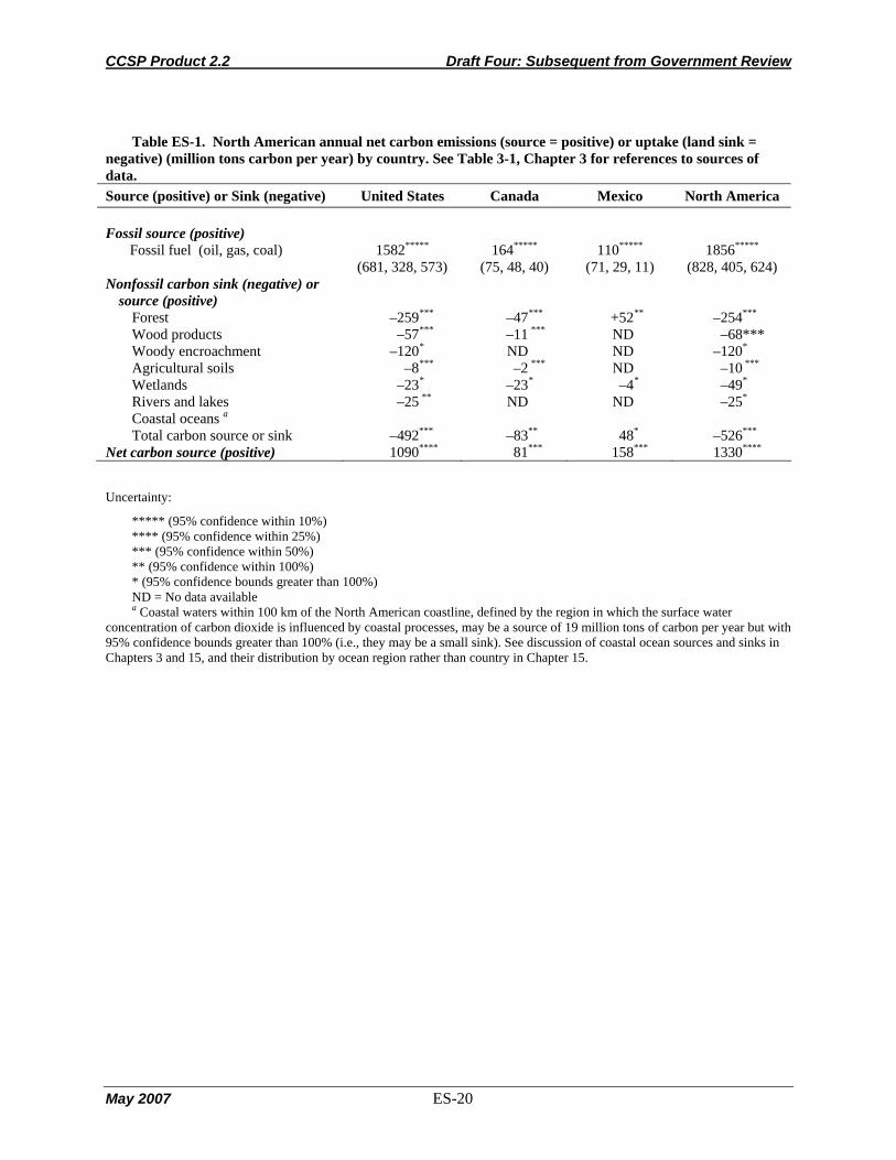
CCSP Product 2.2 Draft Four: Subsequent from Government Review
May 2007 ES-20
Table ES-1. North American annual net carbon emissions (source = positive) or uptake (land sink =
negative) (million tons carbon per year) by country. See Table 3-1, Chapter 3 for references to sources of data. Source (positive) or Sink (negative) United States Canada Mexico North America Fossil source (positive)
Fossil fuel (oil, gas, coal) 1582*****
(681, 328, 573) 164*****
(75, 48, 40) 110*****
(71, 29, 11) 1856*****
(828, 405, 624) Nonfossil carbon sink (negative) or
source (positive)
Forest –259*** –47*** +52** –254***
Wood products –57*** –11 *** ND –68*** Woody encroachment –120* ND ND –120*
Agricultural soils –8*** –2 *** ND –10 ***
Wetlands –23* –23* –4* –49*
Rivers and lakes –25 ** ND ND –25*
Coastal oceans a Total carbon source or sink –492*** –83** 48* –526***
Net carbon source (positive) 1090**** 81*** 158*** 1330****
Uncertainty:
***** (95% confidence within 10%) **** (95% confidence within 25%) *** (95% confidence within 50%) ** (95% confidence within 100%) * (95% confidence bounds greater than 100%) ND = No data available a Coastal waters within 100 km of the North American coastline, defined by the region in which the surface water
concentration of carbon dioxide is influenced by coastal processes, may be a source of 19 million tons of carbon per year but with 95% confidence bounds greater than 100% (i.e., they may be a small sink). See discussion of coastal ocean sources and sinks in Chapters 3 and 15, and their distribution by ocean region rather than country in Chapter 15.

CCSP Product 2.2 Draft Four: Subsequent from Government Review
May 2007 ES-21
Figure ES-1. North American carbon sources and sinks (million tons carbon per year) circa 2003. Height of a bar indicates a best estimate for net carbon exchange between the atmosphere and the indicated element of the North American carbon budget. Sources add carbon dioxide to the atmosphere; sinks remove it. Error bars indicate the uncertainty in that estimate, and define the range of values that include the actual value with 95% certainty. See Chapter 3 and Chapters 6-15 of this report for details and discussion of these sources and sinks.

CCSP Product 2.2 Draft Four: Subsequent from Government Review
May 2007 ES-22
[This page intentionally left blank]
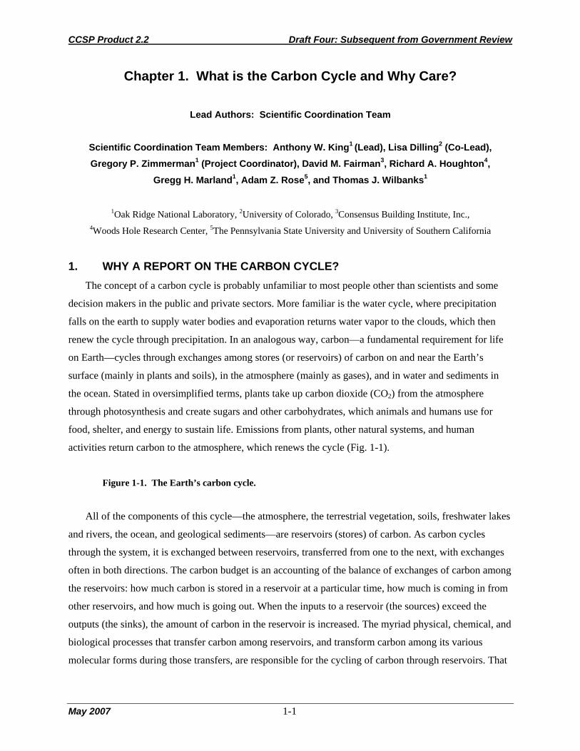
CCSP Product 2.2 Draft Four: Subsequent from Government Review
May 2007 1-1
Chapter 1. What is the Carbon Cycle and Why Care?
Lead Authors: Scientific Coordination Team
Scientific Coordination Team Members: Anthony W. King1 (Lead), Lisa Dilling2 (Co-Lead), Gregory P. Zimmerman1 (Project Coordinator), David M. Fairman3, Richard A. Houghton4,
Gregg H. Marland1, Adam Z. Rose5, and Thomas J. Wilbanks1
1Oak Ridge National Laboratory, 2University of Colorado, 3Consensus Building Institute, Inc.,
4Woods Hole Research Center, 5The Pennsylvania State University and University of Southern California
1. WHY A REPORT ON THE CARBON CYCLE? The concept of a carbon cycle is probably unfamiliar to most people other than scientists and some
decision makers in the public and private sectors. More familiar is the water cycle, where precipitation
falls on the earth to supply water bodies and evaporation returns water vapor to the clouds, which then
renew the cycle through precipitation. In an analogous way, carbon—a fundamental requirement for life
on Earth—cycles through exchanges among stores (or reservoirs) of carbon on and near the Earth’s
surface (mainly in plants and soils), in the atmosphere (mainly as gases), and in water and sediments in
the ocean. Stated in oversimplified terms, plants take up carbon dioxide (CO2) from the atmosphere
through photosynthesis and create sugars and other carbohydrates, which animals and humans use for
food, shelter, and energy to sustain life. Emissions from plants, other natural systems, and human
activities return carbon to the atmosphere, which renews the cycle (Fig. 1-1).
Figure 1-1. The Earth’s carbon cycle.
All of the components of this cycle—the atmosphere, the terrestrial vegetation, soils, freshwater lakes
and rivers, the ocean, and geological sediments—are reservoirs (stores) of carbon. As carbon cycles
through the system, it is exchanged between reservoirs, transferred from one to the next, with exchanges
often in both directions. The carbon budget is an accounting of the balance of exchanges of carbon among
the reservoirs: how much carbon is stored in a reservoir at a particular time, how much is coming in from
other reservoirs, and how much is going out. When the inputs to a reservoir (the sources) exceed the
outputs (the sinks), the amount of carbon in the reservoir is increased. The myriad physical, chemical, and
biological processes that transfer carbon among reservoirs, and transform carbon among its various
molecular forms during those transfers, are responsible for the cycling of carbon through reservoirs. That

CCSP Product 2.2 Draft Four: Subsequent from Government Review
May 2007 1-2
cycling determines the balance of the carbon budget observed at any particular time. Quantifying the
carbon budget over time can reveal whether the budget is or is not in balance (carbon accumulating in a
reservoir would indicate an imbalance). If found to be out of balance, this quantification can provide
understanding about why such a condition exists (for example, which sources exceed which sinks over
what periods) (Sabine et al., 2004, Chapter 2 this report). If the imbalance is deemed undesirable, the
understanding of source and sinks can provide clues into how it might be managed (for example, which
sinks are large relative to sources and might, if managed, provide leverage on changes in a reservoir)
(Caldeira et al., 2004; Chapter 4 this report). The global carbon budget is currently out of balance, with
carbon accumulating in the form of CO2 and methane (CH4) in the atmosphere since the preindustrial era
(circa 1750). Human use of coal, petroleum, and natural gas, combined with agriculture and other land-
use change is primarily responsible. Documented by the Intergovernmental Panel on Climate Change for
the 1990s (IPCC, 2001, p. 4), these trends continue in the early twenty-first century (Keeling and Whorf,
2005; Marland et al., 2006).
The history of the Earth’s carbon balance as reflected in changes in atmospheric CO2 concentration
can be reconstructed from geological records, geochemical reconstructions, measurements on air bubbles
trapped in glacial ice, and in recent decades, direct measurements of the atmosphere. Over the millennia,
tens and hundreds of millions of years ago, vast quantities of carbon were stored in residues from dead
plant and animal life that sank into the earth and became fossilized. On these time scales, small
imbalances in the carbon cycle and geological processes, acting over millions of years, produced large but
slow changes in atmospheric CO2 concentrations of greater than 3000 parts per million (ppm) over
periods of 150-200 million years (Prentice et al., 2001). By perhaps 20 million year ago, atmospheric CO2
concentrations were less than 300 ppm (Prentice et al., 2001). Subsequently, imbalances in the carbon
cycle linked with climate variations, especially the large glacial-interglacial cycles of the last 420,000
years, resulted in changes of approximately 100 ppm over periods of 50-75 thousand years (Prentice et
al., 2001; Sabine et al., 2004). During the current interglacial climate, for at least the last 11,000 years,
variations in atmospheric CO2, also likely climate driven, were less than 20 ppm (Joos and Prentice,
2004). For 800-1000 years prior to the Industrial Revolution of the 1700s and 1800s, atmospheric CO2
concentrations varied by less than 10 ppm (Prentice et al., 2001).
With the advent of the steam engine, the internal combustion engine, and other technological and
economic elements of the Industrial Revolution, human societies found that the fossilized carbon formed
hundreds of millions of years ago had great value as energy sources for economic growth. The 1800s and
1900s saw a dramatic rise in the combustion of these “fossil fuels” (e.g., coal, petroleum, and natural gas),
releasing into the atmosphere, over decades, quantities of carbon that had been stored in the Earth system
over millennia. These fossil-fuel emissions combined with and soon exceeded (circa 1910) the CO2

CCSP Product 2.2 Draft Four: Subsequent from Government Review
May 2007 1-3
emissions from burning and decomposition of dead plant material that accompanied clearing of forests for
agricultural land use (Houghton, 2003).
It is not surprising, then, that measurements of CO2 in the Earth’s atmosphere have shown a steady
increase in concentration over the twentieth century (Keeling and Whorf, 2005). The global CO2
concentration has increased by approximately 100 ppm over the past 200 years, from a preindustrial
concentration of 280 ± 10 ppm (Prentice et al., 2001) to a concentration (measured at Mauna Loa,
Hawaii) of 369 ppm in 2000 and 377 ppm in 2004 (Keeling and Whorf, 2005). Methane shows a similar
pattern, with relatively stable concentrations prior to about 1800 followed by a rapid increase (Ehhalt et
al., 2001). Roughly, 20% of CH4 emissions are from gas released in the extraction and transportation of
fossil fuels; the rest is from biological sources including expanding rice and cattle production (Prinn,
2004). Such large increases in atmospheric carbon over such a short period of time relative to historical
variations, together with patterns of human activity that will likely continue into the twenty-first century,
such as trends in fossil fuel use and tropical deforestation, raises concerns about imbalances in the carbon
cycle and their implications.
2. THE CARBON CYCLE AND CLIMATE CHANGE
Most of the carbon in the Earth’s atmosphere is in the form of CO2 and CH4. Both CO2 and CH4 are
important “greenhouse gases.” Along with water vapor and other “radiatively active” gases in the
atmosphere, they absorb heat radiated from the Earth’s surface, heat that would otherwise be lost into
space. As a result, these gases help to warm the Earth’s atmosphere. Rising concentrations of atmospheric
CO2 and other greenhouse gases can alter the Earth’s radiant energy balance. The Earth’s energy budget
determines the global circulation of heat and water through the atmosphere and the patterns of
temperature and precipitation we experience as weather and climate. Thus, the human disturbance of the
Earth’s global carbon cycle during the Industrial era and the resulting imbalance in the Earth’s carbon
budget and buildup of atmospheric CO2 have consequences for climate and climate change. According to
the Intergovernmental Panel on Climate Change (IPCC), CO2 is the largest single forcing agent of climate
change (IPCC, 2001)1.
1 Methane is also an important contributor (IPCC, 2001). However, CH4 and other non-CO2 carbon gases are not typically included in global carbon budgets because their sources and sinks are not well understood (Sabine et al., 2004). For this reason, and to manage scope and focus, we too follow that convention and this report is limited primarily to the carbon cycle and carbon budget of North America at it influences and is influenced by atmospheric CO2. Methane is discussed in individual chapters where appropriate, but the report makes no effort to provide a comprehensive synthesis and assessment of CH4 as part of the North American carbon budget. Similarly we provide no comprehensive treatment of black carbon, isoprene or other volatile organic carbon compounds that represent a small fraction of global or continental carbon budgets.

CCSP Product 2.2 Draft Four: Subsequent from Government Review
May 2007 1-4
In addition to the relationship between climate change and atmospheric CO2 as a greenhouse gas,
research is beginning to reveal the feedbacks between a changing carbon cycle and changing climate, and
the associated implications for future climate change. Simulations with climate models that include an
interactive global carbon cycle indicate a positive feedback between climate change and atmospheric CO2
concentrations. The magnitude of the feedback varies considerably among models; but in all cases, future
atmospheric CO2 concentrations are higher and temperature increases are larger in the coupled climate-
carbon cycle simulations than in simulations without the coupling and feedback between climate change
and changes in the carbon cycle (Friedlingstein et al., 2006). The research is in its early stages, but 8 of
the 11 models, in a recent comparison among models (Friedlingstein et al., 2006), attributed most of the
feedback to changes in land carbon, with the majority locating those changes in the tropics. Differences
among models in almost every aspect of plant and soil response to climate were responsible for the
differences in model results, including plant growth in response to atmospheric CO2 concentrations and
climate and accelerated decomposition of dead organic matter in response to warmer temperatures.
Changes in temperature, precipitation, and other climate variables also contribute to year-to-year
changes in carbon cycling. Nearly all of the biological, chemical, and physical processes responsible for
exchange of carbon between atmosphere, land, and ocean are influenced to some degree by climate
variables, and both ocean-atmosphere and land-atmosphere exchanges and sources and sinks, show year-
to-year variation attributable to variability in climate (Prentice et al., 2001; Schaefer et al., 2002;
Houghton, 2003; Sabine et al., 2004; Greenblatt and Sarmiento, 2004; Chapter 2 this report). This
variability is believed to be responsible for the large year-to-year differences in the accumulation of CO2
in the atmosphere; annual changes differ by as much as 3000 to 4000 million metric tons of carbon (Mt
C) per year (Prentice et al., 2001; Houghton, 2003). Both land and ocean show changes, for example, in
apparent response to climate conditions linked to El Niño events, although the variability in the net land-
atmosphere exchange is larger (Prentice et al., 2001; Houghton, 2003; Sabine et al., 2004). Figure 1-2
illustrates this variability, showing for North America year-to-year variation in satellite observations of
the annual net transfer of carbon from the atmosphere to plants. Variability of this sort, in both land and
ocean, contributes uncertainty to carbon budgeting and may appear as “noise” when attempting to detect
“signals” of longer-term climate relevant trends (Sabine et al., 2004) or, eventually, signals of effective
carbon management.
Figure 1-2. Variability in net primary production (NPP) for North America from 2000-2005.
Many of the currently proposed options to prevent, minimize, or forestall future climate change will
likely require management of the carbon cycle and concentrations of CO2 in the atmosphere. That

CCSP Product 2.2 Draft Four: Subsequent from Government Review
May 2007 1-5
management includes both reducing sources, such as the combustion of fossil fuels, and enhancing sinks,
such as uptake and storage (sequestration) in vegetation and soils. In either case, the formulation of
options by decision makers and successful management of the Earth’s carbon budget requires solid
scientific understanding of the carbon cycle and the “ability to account for all carbon stocks, fluxes, and
changes and to distinguish the effects of human actions from those of natural system variability” (CCSP,
2003).
So, why care about the carbon cycle? In short, because people care about the potential consequences
of global climate change, they also, necessarily, care about the carbon cycle and the balance between
carbon sources and sinks, natural and human, which determine the budget imbalance and accumulation of
carbon in the atmosphere as CO2.
3. OTHER IMPLICATIONS OF AN IMBALANCE IN THE CARBON BUDGET
The consequences of an unbalanced carbon budget with carbon accumulating in the atmosphere as
CO2 and CH4 are not completely understood, but it is known that they extend beyond climate change
alone. Experimental studies, for example, show that for many plant species, rates of photosynthesis often
increase in response to elevated concentrations of CO2, thus, potentially increasing plant growth and even
agricultural crop yields in the future. There is, however, considerable uncertainty about whether such
“CO2 fertilization” will continue into the future with prolonged exposure to elevated CO2; and, of course,
its potential beneficial effects on plants presume climatic conditions that are also favorable to plant and
crop growth.
It is also increasingly evident that atmospheric CO2 concentrations are responsible for increased
acidity of the surface ocean (Caldeira and Wickett, 2003), with potentially dire future consequences for
corals and other marine organisms that build their skeletons and shells from calcium carbonate. Ocean
acidification is a powerful reason, in addition to climate change, to care about the carbon cycle and the
accumulation of CO2 in the atmosphere (Orr et al., 2005).
4. WHY THE CARBON BUDGET OF NORTH AMERICA?
The continent of North America has been identified as both a significant source and a significant sink
of atmospheric CO2 (IPCC, 2001; Pacala et al. 2001; Goodale et al., 2002; Gurney et al., 2002; EIA,
2005). More than a quarter (27%) of global carbon emissions, from the combination of fossil-fuel burning
and cement manufacturing, are attributable to North America (United States, Canada, and Mexico)
(Marland et al., 2003). North American plants remove CO2 from the atmosphere and store it as carbon in
plant biomass and soil organic matter, mitigating to some degree the human-caused (anthropogenic)
sources. The magnitude of the “North American sink” has been previously estimated at anywhere from

CCSP Product 2.2 Draft Four: Subsequent from Government Review
May 2007 1-6
less than 100 Mt C per year to slightly more than 2000 Mt C per year (Turner et al., 1995; Fan et al.,
1998), with a value near 350 to 750 Mt C per year most likely (Houghton et al., 1999; Goodale et al.,
2002; Gurney et al., 2002). The North American sink is thus, a substantial, if highly uncertain, fraction,
from 15% to essentially 100%, of the extra-tropical Northern Hemisphere terrestrial sink estimated to be
in the range of 600 to 2300 Mt C per year during the 1980s (Prentice et al., 2001). It is also a reasonably
large fraction (perhaps near 30%) of the global terrestrial sink estimated at 1900 Mt C per year for the
1980s (but with a range of uncertainty from a large sink of 3800 Mt C per year to a small source of 300
Mt C per year (Prentice et al., 2001). The global terrestrial sink absorbs approximately one quarter of the
carbon added to the atmosphere by human activities, but with uncertainties linked to the uncertainties in
the size of that sink. Global atmospheric carbon concentrations would be substantially higher than they
are without the partially mitigating influence of the sink in North America. However, estimates of that
sink vary widely, and it needs to be better quantified.
Some mechanisms that might be responsible for the North American terrestrial sink are reasonably
well known. These mechanisms include, but are not limited to, the regrowth of forests following
abandonment of agriculture, changes in fire and other disturbance regimes, historical climate change, and
fertilization of ecosystem production by nitrogen deposition and elevated atmospheric CO2 (Dilling et al.,
2003; Foley et al., 2004). Recent studies have indicated that some of these processes are likely more
important than others for the current North American carbon sink, with regrowth of forests on former
agricultural land generally considered to be a major contributor, and with, perhaps, a significant
contribution from enhanced plant growth in response to higher concentrations of atmospheric CO2 (CO2
fertilization) (Caspersen et al., 2000; Schimel et al., 2000; Houghton, 2002). But significant uncertainties
remain (Caspersen et al., 2000; Schimel et al., 2000; Houghton, 2002), with some arguing that even the
experimental evidence for CO2 fertilization is equivocal at the larger spatial scales necessary for a
significant terrestrial sink (e.g., Nowak et al., 2004; Friedlingstein et al., 2006). The future of the current
North American terrestrial sink is highly uncertain, and it depends on which mechanisms are the
dominant drivers now and in the future.
Estimates of coastal carbon cycling and input of carbon from the land are equally uncertain (Liu et
al., 2000). Coastal processes are also difficult to parameterize in global carbon cycle models, which are
often used to derive best-guess estimates for regional carbon budgets (Liu et al., 2000). It is very
important to quantify carbon fluxes in coastal margins of the area adjacent to the North American
continent, lest regional budgets of carbon on land be misattributed.
North America is a major player in the global carbon cycle, in terms of both sources and sinks.
Accordingly, understanding the carbon budget of North America is a necessary part of understanding the
global carbon cycle. Such understanding is helpful for successful carbon management strategies to

CCSP Product 2.2 Draft Four: Subsequent from Government Review
May 2007 1-7
mitigate fossil-fuel emissions or stabilize concentrations of greenhouse gases in the atmosphere.
Moreover, a large North American terrestrial sink generated by “natural” processes is an ecosystem
service that would be valued at billions of dollars if purchased or realized through direct human economic
and technological intervention. Its existence will likely influence carbon-management decision making,
and it is important that its magnitude and its dynamics be well understood (Kirschbaum and Cowie, 2004;
Canadell et al., 2007).
It is particularly important to understand the likely future behavior of carbon in North America,
including terrestrial and oceanic sources, and sinks. Decisions made about future carbon management
with expectations of the future behavior of the carbon cycle that proved to be significantly in error, could
be costly. For example, future climate-carbon feedbacks could change the strength of terrestrial sinks and
put further pressure on emission reductions to achieve atmospheric stabilization targets (Jones et al.,
2006; Canadell et al., 2007). The future cannot be known, but understanding the current and historical
carbon cycle will increase confidence in projections for appropriate consideration by decision makers.
5. CARBON CYCLE SCIENCE IN SUPPORT OF CARBON MANAGEMENT DECISIONS
Beyond understanding the science of the North American carbon budget and its drivers, increasing
attention is now being given to deliberate management strategies for carbon (DOE, 1997, Hoffert et al.,
2002; Dilling et al., 2003). Carbon management is now being considered at a variety of scales in North
America. There are tremendous opportunities for carbon cycle science to improve decision making in this
arena, whether in reducing carbon emissions from the use of fossil fuels, or in managing terrestrial carbon
sinks. Many decisions in government, business, and everyday life are connected with the carbon cycle.
They can relate to driving forces behind changes in the carbon cycle (such as consumption of fossil fuels)
and strategies for managing them, and/or impacts of changes in the carbon cycle (such as climate change
or ocean acidification) and responses to reduce their severity. Carbon cycle science can help to inform
these decisions by providing timely and reliable information about facts, processes, relationships, and
levels of confidence.
In seeking ways to use scientific information more effectively in decision making, we must pay
particular attention to the importance of developing constructive scientist–stakeholder interactions.
Studies of these interactions all indicate that neither scientific research nor assessments can be assumed to
be relevant to the needs of decision makers if conducted in isolation from the context of those users’
needs (Cash and Clark, 2001; Cash et al., 2003; Dilling et al., 2003; Parson, 2003). Carbon cycle
science’s support of decision making is more likely to be effective if the science connected with

CCSP Product 2.2 Draft Four: Subsequent from Government Review
May 2007 1-8
communication structures is considered by both scientists and users to be legitimate and credible. Well-
designed scientific assessments can be one of these effective communication media.
The climate and carbon research community of North America, and a diverse range of stakeholders,
recognize the need for an integrated synthesis and assessment focused on North America to (a)
summarize what is known and what is known to be unknown, documenting the maturity as well as the
uncertainty of this knowledge; (b) convey this information to scientists and to the larger community; and
(c) ensure that our studies are addressing the questions of concern to society and decision-making
communities. As the most comprehensive synthesis to date of carbon cycle knowledge and trends for
North America, incorporating stakeholder interactions throughout its production2, this report, the First
State of the Carbon Cycle Report (SOCCR), focused on The North American Carbon Budget and
Implications for the Global Carbon Cycle is intended as a step in that direction.
CHAPTER 1 REFERENCES Caldeira, K., and M.E. Wickett, 2003: Anthropogenic carbon and ocean pH. Nature, 425, 365-366.
Caldeira, K., M.G. Morgan, D. Baldocchi, P.G. Brewer, C.-T.A. Chen, G.-J. Nabuurs, N. Nakicenovic, and G.P.
Robertson, 2004: A portfolio of carbon management options. In: The Global Carbon Cycle: Integrating
Humans, Climate, and the Natural World [Field, C.B. and M.R. Raupach (eds.)]. Island Press, Washington, DC,
pp. 103-129.
Canadell, J.G., D. Pataki, R. Gifford, R.A. Houghton, Y. Lou, M.R. Raupach, P. Smith, and W. Steffen, 2007:
Saturation of the terrestrial carbon sink. In: Terrestrial Ecosystems in a Changing World, [Canadell, J.G., D.
Pataki, and L. Pitelka (eds.)]. The IGBP Series. Springer-Verlag, Berlin Heidelberg, pp. 59-78.
Cash, D. and W. Clark, 2001: From Science to Policy: Assessing the Assessment Process. Faculty Research
Working Paper 01-045, Kennedy School of Government, Harvard University, Cambridge, MA. Available at
http://ksgnotes1.harvard.edu/Research/wpaper.nsf/RWP/RWP01-045
Cash, D., W. Clark, F. Alcock, N. Dickson, N. Eckley, D. Guston, J. Jäger, and R. Mitchell, 2003: Knowledge
systems for sustainable development. Proceedings of the National Academy of Sciences, 100, 8086-8091.
Casperson, J.P., S.W. Pacala, J.C. Jenkins, G.C. Hurtt, P.R. Moorcraft, and R.A. Birdsey, 2000: Contributions of
land-use history to carbon accumulation in U.S. Forests. Science, 290, 1148-1151.
CCSP, 2003: Strategic Plan for the U.S. Climate Change Science Program. A Report by the Climate Change
Science Program and the Subcommittee on Global Change Research, Climate Change Science Program Office,
Washington, DC.
DOE, 1997: Technology Opportunities to Reduce Greenhouse Gas Emissions. U.S. Department of Energy,
Washington, DC.
2 A discussion of stakeholder participation in the production of this report can be found in the Preface of this report.

CCSP Product 2.2 Draft Four: Subsequent from Government Review
May 2007 1-9
Dilling, L., S.C. Doney, J. Edmonds, K.R. Gurney, R.C. Harriss, D. Schimel, B. Stephens, and G. Stokes, 2003: The
role of carbon cycle observations and knowledge in carbon management. Annual Review of Environment and
Resources, 28, 521-58.
Ehhalt, D., M. Prather, et al., 2001: Atmospheric chemistry and greenhouse gases. In: Climate Change 2001: The
Scientific Basis (Contribution of Working Group I to the Third Assessment Report of the Intergovernmental
Panel on Climate Change). [Houghton, J. T., Y. Ding, D.J. Griggs, M. Noguer, P. J. van der Linden and D.
Xiaosu (eds.)]. Cambridge University Press, Cambridge, UK and New York, NY, pp. 239-287.
EIA (Energy Information Administration), 2005: Historical Data Overview. U.S. Department of Energy.
Available at http://www.eia.doe.gov/overview_hd.html; http://cdiac.ornl.gov/ftp/trends/emis/meth-reg.htm
Fan, S., M. Gloor, J. Mahlman, S. Pacala, J. Sarmiento, T. Takahashi, and P. Tans, 1998: A large terrestrial carbon
sink in North America implied by atmospheric and oceanic carbon dioxide data and models. Science, 282, 442-
446.
Foley, J.A., N. Ramankutty, 2004: A primer on the terrestrial carbon cycle: What we don’t know but should. In: The
global carbon cycle: Integrating humans, climate and the natural world. [Field, C.B. and M.R. Raupauch,
(eds.)] SCOPE Report 62. Island Press, Washington DC. Pp. 279-294.
Friedlingstein, P., P. Cox, R. Betts, L. Bopp, W. von Bloh, V. Brovkin, S. Doney, M. Eby, I. Fung, B.
Govindasamy, J. John, C. Jones, F. Joos, T. Kato, M. Kawamiya, W. Knorr, K. Lindsay, H.D. Matthews, T.
Raddatz, P. Rayner, C. Reick, E. Roeckner, K.-G. Schnitzler, R. Schnur, K. Strassmann, S. Thompson, A.J.
Weaver, C. Yoshikawa, and N. Zeng, 2006: Climate-carbon cycle feedback analysis, results from the C4MIP
model intercomparison. Journal of Climate, 19, 3337-3353.
Goodale, C.L., M.J. Apps, R.A. Birdsey, C.B. Field, L.S. Heith, R.A. Houghton, J.C. Jenkins, G.H. Kholmaier, W.
Kurz, S. Liu, G.-J. Nabuurs, S. Nilsson, and A.Z. Shvidenko, 2002: Forest carbon sinks in the Northern
Hemisphere. Ecological Applications, 12, 891-899.
Greenblatt, J.B. and J.L. Sarmiento, 2004: Variability and climate feedback mechanisms in ocean uptake of CO2.
In: The Global Carbon Cycle: Integrating Humans, Climate, and the Natural World [Field, C.B. and M.R.
Raupach (eds.)]. Island Press, Washington, DC, pp. 257-275.
Gurney, K.R., R.M. Law, A.S. Denning, P.J. Rayner, D. Baker, P. Bousquet, L. Bruhwiler, Y.-H. Chen, P. Ciais, S.
Fan, I.Y. Fung, M. Gloor, M. Heimann, K. Higuchi, J. John, T. Maki, S. Maksyutov, K. Masarie, P. Peylin, M.
Prather, B.C. Pak, J. Randerson, J. Sarmiento, S. Taguchi, T. Takahashi, and C.-W. Yue, 2002: Towards robust
regional estimates of CO2 sources and sinks using atmospheric transport models. Nature, 415, 626-630.
Hoffert, M.I., K.C. Caldeira, G. Benford, D.R. Criswell, C. Green, H. Herzog, J.W. Katzenberger, H.S. Kheshgi,
K.S. Lackner, J.S. Lewis, W. Manheimer, J.C. Mankins, G. Marland, M.E. Mauel, L.J. Perkins, M.E.
Schlesinger, T. Volk, and T.M.L. Wigley, 2002: Advanced technology paths to global climate stability: energy
for a greenhouse planet. Science, 298, 981-87.
Houghton, R.A., J.L. Hackler, and K.T. Lawrence, 1999: The U.S. carbon budget: contributions from land-use
change. Science, 285, 574-578.
CCSP Product 2.2 Draft Four: Subsequent from Government Review
May 2007 1-10
Houghton, R.A., 2002: Magnitude, distribution and causes of terrestrial carbon sinks and some implications for
policy. Climate Policy, 2, 71-88.
Houghton, R.A., 2003: The contemporary carbon cycle. In: Treatise on Geochemistry, Volume 8 Biogeochemistry
[Schlesinger, W.H. (ed.)]. Elsevier Ltd, New York, pp. 473-513.
IPCC, 2001: Climate Change 2001: Synthesis Report. A Contribution of Working Groups I, II and III to the Third
Assessment Report of the Intergovernmental Panel on Climate Change [Watson, R.T., and the Core Writing
Team (eds.)]. Cambridge University Press, Cambridge, UK, and New York, NY, 398 pp.
Jones, C.D., P.M. Cox, and C. Huntingford, 2006: Climate-carbon cycle feedbacks under stabilization: uncertainty
and observational constraints. Tellus, 58B, 603-613.
Joos, F. and I.C. Prentice, 2004: A paleo-perspective on changes in atmospheric CO2 and climate. In: The Global
Carbon Cycle: Integrating Humans, Climate, and the Natural World [Field, C.B. and M.R. Raupach (eds.)].
Island Press, Washington, DC, pp. 165-186.
Keeling, C.D. and T.P. Whorf, 2005: Atmospheric CO2 records from sites in the SIO air sampling network. In:
Trends: A Compendium of Data on Global Change. Carbon Dioxide Information Analysis Center, Oak Ridge
National Laboratory, U.S. Department of Energy, Oak Ridge, TN, USA.
Kirschbaum, M.U.F. and A.L. Cowie, 2004: Giving credit where credit is due: A practical method to distinguish
between human and natural factors in carbon accounting. Climatic Change, 67, 417-436.
Liu, K.K., K. Iseki, and S.-Y. Chao, 2000: Continental margin carbon fluxes. In: The Changing Ocean Carbon
Cycle [Hansen, R., H.W. Ducklow, and J.G. Field (eds.)]. Cambridge University Press, Cambridge, UK, pp.
187–239.
Marland, G., T.A. Boden, and R.J. Andres, 2003: Global, regional, and national CO2 emissions. In: Trends: A
Compendium of Data on Global Change. Carbon Dioxide Information Analysis Center, Oak Ridge National
Laboratory, Oak Ridge, TN.
Marland, G., T.A. Boden, and R.J. Andres, 2006: Global, Regional, and National CO2 Emissions. In: Trends: A
Compendium of Data on Global Change. Carbon Dioxide Information Analysis Center, Oak Ridge National
Laboratory, U.S. Department of Energy, Oak Ridge, TN, USA.
Nowak, R.S., D.S. Ellsworth, and S.D. Smith, 2004: Functional responses of plants to elevated atmospheric CO2- do
photosynthetic and productivity data from FACE experiments support early predictions? New Phytologist, 162,
253-280.
Orr, J.C., V.J. Fabry, O. Aumont, L. Bopp, S.C. Doney, R. A. Feely, A. Gnanadesikan, N. Gruber, A. Ishida, F.
Joos, R.M. Key, K. Lindsay, E. Maier-Reimer, R. Matear, P. Monfray, A. Mouchet, R.G. Najjar, G.K. Plattner,
K.B. Rodgers, C.L. Sabine, J.L. Sarmiento, R. Schlitzer, R.D. Slater, I. J. Totterdell, M.F. Weirig, Y.
Yamanaka, and A. Yool, 2005: Anthropogenic ocean acidification over the twenty-first century and its impact
on calcifying organisms, Nature, 437, 681-686. Pacala, S.W., G.C. Hurtt, R.A. Houghton, R.A. Birdsey, L. Heath, E.T. Sundquist, R.F. Stallard, D. Baker,
P. Peylin, P. Moorcroft, J. Caspersen, E. Shevliakova, M.E. Harmon, S.-M. Fan, J.L. Sarmiento, C. Goodale,
C.B. Field, M. Gloor, and D. Schimel, 2001: Consistent land- and atmosphere-based U.S. carbon sink estimates.

CCSP Product 2.2 Draft Four: Subsequent from Government Review
May 2007 1-11
Science, 292(5525), 2316–2320.
Parson, E.A., 2003: Protecting the Ozone Layer. Oxford University Press, Oxford, UK.
Prentice, I.C., et al., 2001: The carbon cycle and atmospheric carbon dioxide. In: Climate Change 2001: The
Scientific Basis (Contribution of Working Group I to the Third Assessment Report of the Intergovernmental
Panel on Climate Change). [Houghton, J.T., Y. Ding, D.J. Griggs, M. Noguer, P.J. van der Linden and D.
Xiaosu (eds.)]. Cambridge University Press, Cambridge, UK and New York, NY, pp. 183-237.
Prinn, R.G., 2004: Non-CO2 greenhouse gases. In: The Global Carbon Cycle: Integrating Humans, Climate, and
the Natural World [Field, C.B. and M.R. Raupach (eds.)]. Island Press, Washington, DC, pp. 205-216.
Running, S.W., R.R. Nemani, F.A. Heinsch, M. Zhao, M. Reeves, and H. Hashimoto, 2004: A continuous satellite-
derived measure of global terrestrial primary production. BioScience, 54, 547-560.
Sabine, C.L., M. Heiman, P. Artaxo, D.C.E. Bakker, C.-T.A. Chen, C.B. Field, N. Gruber, C. LeQuéré, R.G. Prinn,
J.E.Richey, P. Romero-Lankao, J.A. Sathaye, and R. Valentini, 2004: Current status and past trends of the
carbon cycle. In: The Global Carbon Cycle: Integrating Humans, Climate, and the Natural World [Field, C.B.
and M.R. Raupach (eds.)]. Island Press, Washington, DC, pp. 17-44.
Schaefer, K., A.S. Denning, N. Suits, J. Kaduk, I. Baker, S. Los, and L. Prihodko, 2002: Effect of climate on
interannual variability of terrestrial CO2 fluxes. Global Biogeochemical Cycles, 16, 1102,
doi:10.1029/2002GB001928.
Schimel, D.S., J. Melillo, H. Tian, A.D. McGuire, D. Kicklighter, T. Kittel, N. Rosenbloom, S. Running, P.
Thornton, D. Ojima, W. Parton, R. Kelly, M. Sykes, R. Neilson, and B. Rizzo, 2000: Contribution of increasing
CO2 and climate to carbon storage by ecosystems in the United States. Science, 287, 2004-2006.
Sundquist, E.T. and K. Visser, 2003: The geological history of the carbon cycle. In: Treatise on Geochemistry,
Volume 8 Biogeochemistry [Schlesinger, W.H. (ed.)]. Elsevier Ltd, New York, pp. 425-472.
Turner, D.P., G.J. Koerper, M.E. Harmon, and J.J. Lee, 1995: A carbon budget for forests of the conterminous
United States. Ecological Applications, 5, 421-436.

CCSP Product 2.2 Draft Four: Subsequent from Government Review
May 2007 1-12
[START OF TEXT BOX]
The Earth’s Carbon Cycle The burning of fossil fuels transfers carbon from geological reservoirs of coal, oil, and gas and releases carbon
dioxide into the atmosphere. Tropical deforestation and other changes in land use also release carbon to the
atmosphere as vegetation is burned and dead material decays. Photosynthesis transfers carbon dioxide from the
atmosphere and the carbon is stored in wood and other plant tissues. The respiration that accompanies plant
metabolism transfers some of the carbon back to the atmosphere as carbon dioxide. When plants die, their decay
also releases carbon dioxide to the atmosphere. A fraction of the dead organic material is resistant to decay and that
carbon accumulates in the soil. Chemical and physical processes are responsible for the exchange of carbon dioxide
across the sea surface. The small difference between the flux into and out of the surface ocean is responsible for net
uptake of carbon dioxide by the ocean. Phytoplankton, small plants floating in the surface ocean, use carbon
dissolved in the water to build tissue and calcium carbonate shells. When they die, they begin to sink and decay. As
they decay, most of the carbon is redissolved into the surface water, but a fraction sinks into the deeper ocean, the
so-called “biological pump”, eventually reaching the ocean sediments. Currents within the ocean also circulate
carbon from surface waters to the deep ocean and back. Carbon accumulated in soils and ocean sediments millions
of years of ago was slowly transformed to produce the geological reservoirs of today’s fossil fuels. For a more
detailed, quantitative description, see Prentice et al. (2001), Houghton (2003), Sundquist and Visser (2003), Sabine
et al. (2004) and Chapter 2 of this report.
[END OF TEXT BOX]

CCSP Product 2.2 Draft Four: Subsequent from Government Review
May 2007 1-13
Figure 1-1. The Earth’s carbon cycle. Carbon cycles through pools or reservoirs of carbon on land, in the ocean, and in sedimentary rock formations over daily, seasonal, annual, millennial, and geological time scales. See the accompanying text box. Figure adapted from http://www.esd.ornl.gov/iab/iab2-2.htm.
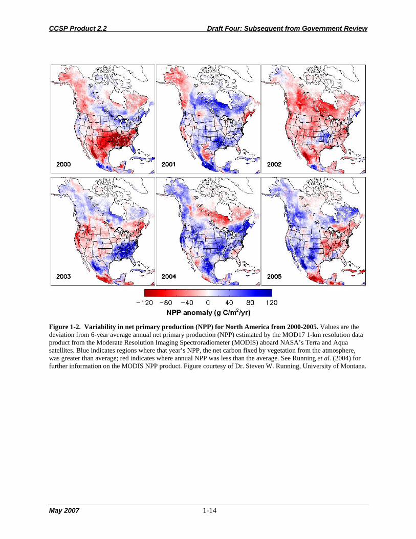
CCSP Product 2.2 Draft Four: Subsequent from Government Review
May 2007 1-14
Figure 1-2. Variability in net primary production (NPP) for North America from 2000-2005. Values are the deviation from 6-year average annual net primary production (NPP) estimated by the MOD17 1-km resolution data product from the Moderate Resolution Imaging Spectroradiometer (MODIS) aboard NASA’s Terra and Aqua satellites. Blue indicates regions where that year’s NPP, the net carbon fixed by vegetation from the atmosphere, was greater than average; red indicates where annual NPP was less than the average. See Running et al. (2004) for further information on the MODIS NPP product. Figure courtesy of Dr. Steven W. Running, University of Montana.

CCSP Product 2.2 Draft Four: Subsequent from Government Review
May 2007 2-1
Chapter 2. The Carbon Cycle of North America in a Global Context
Coordinating Lead Author: Christopher B. Field1
Lead Authors: Jorge Sarmiento2 and Burke Hales3
1Carnegie Institution, 2Princeton University, 3Oregon State University
KEY FINDINGS
• Human activity over the last two centuries, including combustion of fossil fuel and clearing of forests,
has led to a dramatic increase in the concentration of atmospheric carbon dioxide. Global
atmospheric carbon dioxide concentrations have risen by 31% since 1850, and they are now higher
than they have been for 420,000 years.
• North America is responsible for approximately 25% of the emissions produced globally in 2004 by
fossil-fuel combustion, with the United States accounting for 86% of the North American total.
• Human-caused emissions (a carbon source) dominate the carbon budget of North America. Largely
unmanaged, unintentional processes reduce the amount of carbon being removed from the
atmosphere (i.e. a smaller carbon sink/less uptake of carbon). Based on atmospheric inversion
studies, that sink (970 ± 360 Mt C per year) is approximately 50% of the North American emissions,
13% of global fossil-fuel emissions, and approximately 50% of the global terrestrial sink inferred from
global budget analyses and atmospheric inversions. Based on the inventories used in this Report and
an estimated sink of 530 ± 265 Mt C per year, those numbers are 30%, 7% and 30%, respectively.
• While the future trajectory of carbon sinks in North America is uncertain (substantial climate change
could convert current sinks into sources), it is clear that the carbon cycle of the next few decades will
be dominated by the large sources from fossil-fuel emissions.
• Because North American carbon emissions are at least a quarter of global emissions, a reduction in
North American emissions would have global consequences.
1. THE GLOBAL CARBON CYCLE
The modern global carbon cycle is a collection of many different kinds of processes, with diverse
drivers and dynamics, that transfer carbon among major pools in rocks, fossil fuels, the atmosphere, the
oceans, and plants and soils on land (Sabine et al., 2004b) (Fig. 2-1). During the last two centuries,
human actions, especially the combustion of fossil fuel and the clearing of forests, have altered the global
carbon cycle in important ways. Specifically, these actions have led to a rapid, dramatic increase in the

CCSP Product 2.2 Draft Four: Subsequent from Government Review
May 2007 2-2
concentration of carbon dioxide (CO2) in the atmosphere (Fig. 2-2), changing the radiation balance of the
Earth (Hansen et al., 2005), and most likely warming the planet (Mitchell et al., 2001). The cause of the
recent increase in atmospheric CO2 is confirmed beyond a reasonable doubt (Prentice, 2001). This does
not imply, however, that the other components of the carbon cycle have remained unchanged during this
period. In fact, the background, or unmanaged parts, of the carbon cycle have changed dramatically over
the past two centuries. The consequence of these changes is that only about 40% ± 15%† of the CO2
emitted to the atmosphere from fossil-fuel combustion and forest clearing has remained there (Sabine et
al., 2004b). In essence, human actions have received a large subsidy from the unmanaged parts of the
carbon cycle. This subsidy has sequestered, or hidden from the atmosphere, approximately 299 ± 160
billion tons (gigatons [Gt]) of carbon.1
Figure 2-1. Schematic representation of the components of the global carbon cycle.
Figure 2-2. Atmospheric CO2 concentration from 1750 to 2005.
The recent subsidy, or sequestration, of carbon by the unmanaged parts of the carbon cycle, makes
them critical for an accurate understanding of climate change. Future increases in carbon uptake in the
unmanaged parts of the cycle could moderate the risks from climate change, while decreases or transitions
from uptake to release could amplify the risks, perhaps dramatically.
In addition to its role in the climate, the carbon cycle intersects with a number of critical Earth system
processes. Because plant growth is essentially the removal of CO2 from the air through photosynthesis,
agriculture and forestry contribute important fluxes. Wildfire is a major release of carbon from plants and
soils to the atmosphere (Sabine et al., 2004b). The increasing concentration of CO2 in the atmosphere has
already made the world’s oceans more acid (Caldeira and Wickett, 2003). Future changes could
dramatically alter the composition of ocean ecosystems (Feely et al., 2004; Orr et al., 2005).
1.1 The Unmanaged Global Carbon Cycle The modern background, or unmanaged, carbon cycle includes the processes that occur in the absence
of human actions. However, these processes are currently so altered by human influences on the carbon
† Most of the uncertainty in this number is due to the approximately 100% uncertainty in carbon lost from forest clearing. This includes uncertainties in areas deforested, in conditions at the time of deforestation, and in fate following deforestation (Houghton, 1999). Except where otherwise noted, the uncertainty bounds on the numbers in this chapter are expert assessments by the authors of the cited literature, based on synthesizing a wide range of empirical and modeling studies. The details of the approaches to assessing uncertainty are discussed in the literature cited. 1 Throughout this chapter, the pools and fluxes in the carbon cycle are presented in Gt C [1 Gt = 1 billion tons or 1 × 10¹⁵ g]. The mass of CO2 is greater than the mass of carbon by the ratio of their molecular weights, 44/12 or 3.67 times; 1 km3 of coal contains approximately 1 Gt C.

CCSP Product 2.2 Draft Four: Subsequent from Government Review
May 2007 2-3
cycle that it is not appropriate to label them natural. This background part of the carbon cycle is
dominated by two pairs of gigantic fluxes with annual uptake and release that are close to balanced
(Sabine et al., 2004b) (Fig. 2-1). The first of these comprises the terrestrial carbon cycle: plant growth on
land annually fixes about 57 ± 9 Gt of atmospheric carbon, approximately ten times the annual emission
from fossil-fuel combustion, into carbohydrates. Respiration by land plants, animals, and
microorganisms, which provides the energy for growth, activity, and reproduction, returns a slightly
smaller amount to the atmosphere. Part of the difference between photosynthesis and respiration is burned
in wildfires, and part is stored as plant material or soil organic carbon. The second comprises the ocean
carbon cycle: about 92 Gt of atmospheric carbon dissolves annually in the oceans, and about 90 Gt per
year moves from the oceans to the atmosphere (While the gross fluxes have a substantial uncertainty, the
difference is known to within ± 0.2 Gt).2 These air-sea fluxes are driven by cycling within the oceans that
governs exchanges between pools of dissolved CO2, bicarbonate (HCO3), carbonate (CO3), organic
matter, and calcium carbonate.
Before the beginning of the industrial revolution, carbon uptake and release through these two pairs
of large fluxes were almost balanced, with carbon uptake on land approximately 0.45 ± 0.18 Gt C per
year transferred to the oceans by rivers and released from the oceans to the atmosphere (Jacobson et al.,
2007). As a consequence, the level of CO2 in the atmosphere varied by less than 25 ppm in the 10,000
years prior to 1850 (Joos and Prentice, 2004). However, atmospheric CO2 was not always so stable.
During the preceding 420,000 years, atmospheric CO2 was 180-200 ppm during ice ages and
approximately 275 ppm during interglacial periods (Petit et al., 1999). The lower ice-age concentrations
in the atmosphere most likely reflect a transfer of carbon from the atmosphere to the oceans, possibly
driven by changes in ocean circulation and sea-ice cover (Sigman and Boyle, 2000; Keeling and
Stephens, 2001). Enhanced biological activity in the oceans, stimulated by increased delivery of iron-rich
terrestrial dust, may have also contributed to this increased uptake (Martin, 1990).
In the distant past, the global carbon cycle was out of balance in a different way. Fossil fuels are the
product of prehistorically stored plant growth, especially 354 to 290 million years ago in the
Carboniferous period. During this time, luxuriant plant growth and geological activity combined to bury a
small fraction of each year’s growth. Over millions of years, this gradual burial led to the accumulation of
vast stocks of fossil fuel. The total accumulation of fossil fuels is uncertain, but probably in the range of
6000 ± 3000 Gt (Sabine et al., 2004b). This burial of carbon also led to a near doubling of atmospheric
oxygen (Falkowski et al., 2005).
2 This uncertainty is one-half the range among the subset of the 19 Ocean Carbon-Cycle Model Intercomparison Project (OCMIP) models that are consistent with the available 14C and CFC-11 data (Matsumoto et al., 2004).

CCSP Product 2.2 Draft Four: Subsequent from Government Review
May 2007 2-4
1.2 Human-Induced Perturbations to the Carbon Cycle
Since the beginning of the industrial revolution, there has been a massive release of carbon from
fossil-fuel combustion and deforestation. Cumulative carbon emissions from fossil-fuel combustion,
natural gas flaring, and cement manufacturing from 1751 through 2003 are 304 ± 30 Gt (Marland and
Rotty, 1984; Andres et al., 1999; updates through 2003 available at
http://cdiac.ornl.gov/trends/emis/tre_glob.htm). Land-use change from 1850 to 2003, mostly from forest
clearing, added another 162 ± 160 Gt (DeFries et al., 1999; Houghton, 1999; updates through 2000
available at http://cdiac.ornl.gov/trends/landuse/houghton/houghton.html. The total through 2003 was
extrapolated based on the assumption that the annual fluxes in 2001-2003 were the same as in 2000). The
rate of fossil-fuel consumption in any recent year would have required, for its production, more than 400
times the current global primary production (total plant growth) of the land and oceans combined (Dukes,
2003). This has led to a rapid increase in the concentration of CO2 in the atmosphere since the mid-1800s,
with atmospheric CO2 rising by 31% (i.e., from 287 ppm to 375 ppm in 2003; the increase from the mid-
1700s was 35%).
In 2004, the three major countries of North America (Canada, Mexico, and the United States)
together accounted for carbon emissions from fossil-fuel combustion of approximately 1.88 ± 0.2 Gt C,
(about 25%) of the global total.3 The United States, the world’s largest emitter of carbon dioxide, was
responsible for 86% of the North American total. Per capita emissions in 2004 were 5.5 ± 0.5 metric tons
in the United States, 4.9 ± 0.5 metric tons in Canada, and 1.0 ± 0.1 metric tons in Mexico. Per capita
emissions in the United States were nearly 5 times the world average, 2.5 times the per capita emissions
for Western Europe, and more than 8 times the average for Asia and Oceania (DOE EIA, 2006). The
world’s largest countries, China and India, have total carbon emissions from fossil-fuel combustion and
the flaring of natural gas that, though growing rapidly, are lower than those in the United States. The 2004
total for China was 80% of that in the United States, and the total for India was 18% of that in the United
States. Per capita emissions for China and India in 2004 were 18% and 5%, respectively, of the United
States rate (DOE EIA, 2006).
2. ASSESSING GLOBAL AND REGIONAL CARBON BUDGETS
Changes in the carbon content of the oceans and plants and soils on land can be evaluated with at
least five different approaches—flux measurements, inventories, inverse estimates based on atmospheric
CO2, process models, and calculation as a residual. The first method, direct measurement of carbon flux,
is well developed over land for measurements over the spatial scale of up to 1 km2, using the eddy flux
3 Uncertainties in national and per capita emissions are based on data reported by individual countries.

CCSP Product 2.2 Draft Four: Subsequent from Government Review
May 2007 2-5
technique (Wofsy et al., 1993; Baldocchi and Valentini, 2004). Although eddy flux measurements are
now collected at more than 100 networked sites, spatial scaling presents formidable challenges due to
spatial heterogeneity. To date, estimates of continental-scale fluxes based on eddy flux must be regarded
as preliminary. Over the oceans, eddy flux is possible (McGillis, 2001), but estimates based on air-sea
CO2 concentration difference are more widely used (Takahashi et al., 1997).
Inventories, based on measuring trees on land (Birdsey and Heath, 1995) or carbon in ocean-water
samples (Takahashi et al., 2002; Sabine et al., 2004a) can provide useful constraints on changes in the
size of carbon pools, though their utility for quantifying short-term changes is limited. Inventories were
the foundation of the recent conclusion that 118 ± 19 Gt of human-caused carbon entered the oceans
through 1994 (Sabine et al., 2004a) and that forests in the mid-latitudes of the Northern Hemisphere
absorbed and stored 0.6 to 0.7 Gt C per year in the 1990s (Goodale et al., 2002). Changes in the
atmospheric inventory of oxygen (O2) (Keeling et al., 1996) and carbon-13 (13C) in CO2 (Siegenthaler and
Oeschger, 1987) provide a basis for partitioning CO2 flux into land and ocean components.
Process models and inverse estimates based on atmospheric CO2 (or CO2 in combination with 13C or
O2) also provide useful constraints on carbon stocks and fluxes. Process models build from understanding
the underlying principles of atmosphere/ocean or atmosphere/ecosystem carbon exchange to make
estimates over scales of space and time that are relevant to the global carbon cycle. For the oceans,
calibration against observations with tracers (e.g., carbon-14 [14C] and chlorofluorocarbons) (Broecker et
al., 1980) tends to nudge a wide range of models toward similar results. Sophisticated models with
detailed treatment of the ocean circulation, chemistry, and biology all reach about the same estimate for
the current ocean carbon sink, 1.5 to 1.8 Gt C per year (Greenblatt and Sarmiento, 2004) and are in
quantitative agreement with data-inventory approaches. Models of the land carbon cycle take a variety of
approaches. They differ substantially in the data used as constraints, in the processes simulated, and in the
level of detail (Cramer et al., 1999; Cramer et al., 2001). Models that take advantage of satellite data have
the potential for comprehensive coverage at high spatial resolution (Running et al., 2004), but only over
the time domain with available satellite data. Flux components related to human activities, deforestation,
for example, have been modeled based on historical land use (Houghton et al., 1999). At present, model
estimates are uncertain enough that they are often used most effectively in concert with other kinds of
estimates (e.g., Peylin et al., 2005).
Inverse estimates based on atmospheric gases (CO2, 13C in CO2, or O2) infer surface fluxes based on
the spatial and temporal pattern of atmospheric gas concentration, coupled with information on
atmospheric transport (Newsam and Enting, 1988). The atmospheric concentration of CO2 is now
measured with high precision at approximately 100 sites worldwide, with many of the stations added in
the last decade (Masarie and Tans, 1995). The 13C in CO2 and high-precision O2 are measured at far fewer
CCSP Product 2.2 Draft Four: Subsequent from Government Review
May 2007 2-6
sites. The basic approach is a linear Bayesian inversion (Tarantola, 1987; Enting, 2002), with many
variations in the time scale of the analysis, the number of regions used, and the transport model.
Inversions have more power to resolve year-to-year differences than mean fluxes (Rodenbeck et al., 2003;
Baker et al., 2006). Limitations in the accuracy of atmospheric inversions come from the limited density
of concentration measurements (especially in the tropics), uncertainty in the transport, and errors in the
inversion process (Baker et al. 2006). Recent studies that use a number of sets of CO2 monitoring stations
(Rodenbeck et al. 2003), models (Gurney et al., 2003; Law et al., 2003; Gurney et al., 2004; Baker et al.,
2006), temporal scales, and spatial regions (Pacala et al., 2001), highlight the sources of the uncertainties
and appropriate steps for managing them.
A final approach to assessing large-scale CO2 fluxes is solving as a residual. At the global scale, the
net flux to or from the land is often calculated as the residual left after accounting for fossil-fuel
emissions, atmospheric increase, and ocean uptake (Post et al., 1990). Increasingly, the need to treat the
land as a residual is receding, as the other methods improve. Still, the existence of constraints at the level
of the overall budget provides an important connection with reality.
3. RECENT DYNAMICS OF THE UNMANAGED CARBON CYCLE Of the approximately 466 ± 160 Gt C added to the atmosphere by human actions through 2003, only
about 187 ± 5 Gt remain. The “missing carbon” must be stored, at least temporarily, in the oceans and in
ecosystems on land. Based on a recent ocean inventory, 118 ± 19 Gt of the missing carbon was in the
oceans, as of 1994 (Sabine et al., 2004a). Extending this calculation, based on recent sinks (Takahashi et
al., 2002; Gloor et al., 2003; Gurney et al., 2003; Matear and McNeil, 2003; Matsumoto et al., 2004),
leads to an estimate of 137 ± 24 Gt C through 2003. This leaves about 162 ± 160 Gt that must be stored
on land (with most of the uncertainty due to the uncertainty in emissions from land use). Identifying the
processes responsible for the uptake on land, their spatial distribution, and their likely future trajectory
has been one of the major goals of carbon cycle science over the last decade.
Much of the recent research on the global carbon cycle has focused on annual fluxes and their spatial
and temporal variation. The temporal and spatial patterns of carbon flux provide a pathway to
understanding the underlying mechanisms. Based on several different approaches, carbon uptake by the
oceans averaged 1.7 ± 0.2 Gt C per year 4 for the period from 1992-1996 (Takahashi et al., 2002; Gloor et
al., 2003; Gurney et al., 2003; Matear and McNeil, 2003; Matsumoto et al., 2004). The total human-
caused flux is this amount, plus 0.45 Gt per year of preindustrial outgasing, for a total of 2.2 ± 0.4 Gt per
year. This rate represents an integral over high-latitude areas which are gaining carbon, and the tropics,
4 This uncertainty is one-half the range among the subset of the 19 Ocean Carbon-Cycle Model Intercomparison Project (OCMIP) models that are consistent with the available 14C and CFC-11 data (Matsumoto et al., 2004).

CCSP Product 2.2 Draft Four: Subsequent from Government Review
May 2007 2-7
which are losing carbon (Takahashi et al., 2002; Gurney et al., 2003; Gurney et al., 2004; Jacobson et al.,
2007). Interannual variability in the ocean sink for CO2, though substantial (Greenblatt and Sarmiento,
2004), is much smaller than interannual variability on the land (Baker et al., 2006).
In the 1990s, carbon releases from land-use change were more than balanced by ecosystem uptake,
leading to a net sink on land (without accounting for fossil-fuel emissions) of 1.1 ± 1.5 Gt C per year
(Schimel et al., 2001; Sabine et al., 2004b). The dominant sources of recent interannual variation in the
net land flux were El Niño and the eruption of Mount Pinatubo in 1991 (Bousquet et al., 2000;
Rodenbeck et al., 2003; Baker et al., 2006), with most of the year-to-year variation in the tropics (Fig. 2-
3). Fire likely plays a large role in this variability (van der Werf et al., 2004).
Figure 2-3. The 13-model mean CO2 flux interannual variability (Gt C per year) for several
continents (solid lines) and ocean basins (dashed lines).
On a time scale of thousands of years, the ocean will be the sink for more than 90% of the carbon
released to the atmosphere by human activities (Archer et al., 1998). The rate of CO2 uptake by the
oceans is, however, limited. Carbon dioxide enters the oceans by dissolving in seawater. The rate of this
process is determined by the concentration difference between the atmosphere and the surface waters and
by an air-sea exchange coefficient related to wave action, wind, and turbulence (Le Quéré and Metzl,
2004). Because the surface waters represent a small volume with limited capacity to store CO2, the major
control on ocean uptake is at the level of moving carbon from the surface to intermediate and deep waters.
Important contributions to this transport come from the large-scale circulation of the oceans, especially
the sinking of cold water in the Southern Ocean and, to a lesser extent, the North Atlantic.
On land, numerous processes contribute to carbon storage and carbon loss. Some of these are directly
influenced through human actions (e.g., the planting of forests, conversion to no-till agriculture, or the
burying of organic wastes in landfills). The human imprint on others is indirect. This category includes
ecosystem responses to climate change (e.g., warming and changes in precipitation), changes in the
composition of the atmosphere (e.g., increased CO2 and increased tropospheric ozone), and delayed
consequences of past actions (e.g., regrowth of forests after earlier harvesting). Early analyses of the
global carbon budget (e.g., Bacastow and Keeling, 1973) typically assigned all of the net flux on land to a
single mechanism, especially fertilization of plant growth by increased atmospheric CO2. Recent evidence
emphasizes the diversity of mechanisms.

CCSP Product 2.2 Draft Four: Subsequent from Government Review
May 2007 2-8
3.1 The Carbon Cycle of North America The land area of North America is a large source of carbon, but the residual (without emissions from
fossil-fuel combustion) is, by most estimates, currently a sink for carbon. This conclusion for the
continental scale is based mainly on the results of atmospheric inversions. Several studies address the
carbon balance of particular ecosystem types (e.g., forests [Kurz and Apps, 1999; Goodale et al., 2002;
Chen et al., 2003]). Pacala and colleagues (2001) used a combination of atmospheric and land-based
techniques to estimate that the 48 contiguous United States are currently a carbon sink of 0.3 to 0.6 Gt C
per year. This estimate and a discussion of the processes responsible for recent sinks in North America are
updated in Chapter 3 of this report. Based on inversions using 13 atmospheric transport models, North
America was a carbon sink of 0.97 ± 0.36 Gt C per year from 1991-2000 (Baker et al., 2006).5 Over the
area of North America, this amounts to an annual carbon sink of 39.6 g C per square meter per year
similar to the sink inferred for all northern lands (North America, Europe, Boreal Asia, and Temperate
Asia) of 32.5 g C per square meter per year (Baker et al., 2006).
Very little of the current carbon sink in North America is a consequence of deliberate action to absorb
and store (sequester) carbon. Some is a collateral benefit of steps to improve land management, for
increasing soil fertility, improving wildlife habitat, etc. Much of the current sink is unintentional, a
consequence of historical changes in technologies and preferences in agriculture, transportation, and
urban design.
4. CARBON CYCLE OF THE FUTURE
The future trajectory of carbon sinks in North America is very uncertain. Several trends will play a
role in determining the sign and magnitude of future changes. One important controller is the magnitude
of future climate changes. If the climate warms significantly, much of the United States could experience
drought-related decreases in plant growth and an increase in the risk of wildfire (Bachelet et al., 2003),
especially if the warming is not associated with substantial increases in precipitation. Exactly this
pattern—substantial warming with little or no change in precipitation—characterizes North America in
many of the newer climate simulations (Rousteenoja et al., 2003). If North American ecosystems are
sensitive to elevated CO2, nitrogen deposition, or warming, plant growth could increase (Schimel et al.,
2000). The empirical literature on CO2 and nitrogen deposition is mixed, with some reports of substantial
growth enhancement (Norby et al., 2005) and others reporting small or modest effects (Oren et al., 2001;
Shaw et al., 2002; Heath et al., 2005).
5 This uncertainty is a sample standard deviation across monthly output from 13 models.
CCSP Product 2.2 Draft Four: Subsequent from Government Review
May 2007 2-9
Overall, the carbon budget of North America is dominated by carbon releases from the combustion of
fossil fuels. Recent sinks, largely from carbon uptake in plants and soils, may approach 50% of the recent
fossil-fuel source (Baker et al., 2006). Most of this uptake appears to be a rebound, as natural and
managed ecosystems recover from past disturbances. Little evidence supports the idea that these
ecosystem sinks will increase in the future. Substantial climate change could convert current sinks into
sources (Gruber et al., 2004).
In the future, trends in the North American energy economy may intersect with trends in the natural
carbon cycle. A large-scale investment in afforestation could offset substantial future emissions (Graham,
2003). However, costs of this kind of effort would include loss of the new-forested area from its previous
uses (including grazing or agriculture), the energy costs of managing the new forests, and any increases in
emissions of non-CO2 greenhouse gases from the new forests. Large-scale investments in biomass energy
(energy produced from vegetative matter) would have similar costs but would result in offsetting
emissions from fossil-fuel combustion, rather than sequestration (Giampietro et al., 1997). The relative
costs and benefits of investments in afforestation and biomass energy will require careful analysis
(Kirschbaum, 2003). Investments in other energy technologies, including wind and solar, will require
some land area, but the impacts on the natural carbon cycle are unlikely to be significant or widespread
(Hoffert et al., 2002; Pacala and Socolow, 2004).
Like the present, the carbon cycle of North America during the next several decades will be
dominated by fossil-fuel emissions. Deliberate geological sequestration may become an increasingly
important component of the budget sheet. Still, progress in controlling the net release to the atmosphere
must be centered on the production and consumption of energy rather than the processes of the
unmanaged carbon cycle. North America has many opportunities to decrease emissions (Chapter 4 this
report). Nothing about the status of the unmanaged carbon cycle provides a justification for assuming that
it can compensate for emissions from fossil-fuel combustion.
CHAPTER 2 REFERENCES Andres, R.J., D.J. Fielding, G. Marland, T.A. Boden, N. Kumar, and A.T. Kearney, 1999: Carbon dioxide emissions
from fossil-fuel use, 1751-1950. Tellus Series B Chemical and Physical Meteorology, 51, 759-765.
Archer, D., H. Kheshgi, and E. Maier-Reimer, 1998: Dynamics of fossil fuel CO2 neutralization by marine CaCO3.
Global Biogeochemical Cycles, 12, 259-276.
Bacastow, R. and C.D. Keeling, 1973: Atmospheric carbon dioxide and radiocarbon in the natural carbon cycle. II.
Changes from A.D. 1700 to 2070 as deduced from a geochemical reservoir. In: Carbon and the Biosphere
[Woodwell, G.M. and E.V. Pecan (eds.)]. U.S. Department of Commerce, Springfield, VA, pp. 86-135.

CCSP Product 2.2 Draft Four: Subsequent from Government Review
May 2007 2-10
Bachelet, D., R.P. Neilson, T. Hickler, R.J. Drapek, J.M. Lenihan, M.T. Sykes, B. Smith, S. Sitch, and K. Thonicke,
2003: Simulating past and future dynamics of natural ecosystems in the United States. Global Biogeochemical
Cycles, 17, 1045.
Baker, D.F., R.M. Law, K.R. Gurney, P. Rayner, P. Peylin, A.S. Denning, P. Bousquet, L. Bruhwiler, Y.H. Chen, P.
Ciais, I.Y. Fung, M. Heimann, J. John, T. Maki, S. Maksyutov, K. Masarie, M. Prather, B. Pak, S. Taguchi, and
Z. Zhu, 2006: TransCom 3 inversion intercomparison: impact of transport model errors on the interannual
variability of regional CO2 fluxes, 1988-2003. Global Biogeochemical Cycles, 20, GB1002.
Baldocchi, D. and R. Valentini, 2004: Geographic and temporal variation of carbon exchange by ecosystems and
their sensitivity to environmental perturbations. In: The Global Carbon Cycle: Integrating Humans, Climate,
and the Natural World [Field, C.B. and M.R. Raupach (eds.)]. Island Press, Washington, DC, pp. 295-316.
Birdsey, R.A. and L.S. Heath, 1995: Carbon changes in U.S. forests. In: Productivity of America's Forests and
Climate Change [Joyce, L.A. (ed.)]. General Technical Report RM-GTR-271, U.S. Department of Agriculture,
Forest Service, Rocky Mountain Forest and Range Experiment Station, Fort Collins, CO, pp. 56-70.
Bousquet, P., P. Peylin, P. Ciais, C.L. Quéré, P. Friedlingstein, and P.P. Tans, 2000: Regional changes in carbon
dioxide fluxes of land and oceans since 1980. Science, 290, 1342-1346.
Broecker, W.S., T.H. Peng, and T. Takahashi, 1980: A strategy for the use of bomb-produced radiocarbon as a
tracer for the transport of fossil fuel CO2 into the deep-sea source regions. Earth and Planetary Science Letters,
49, 463-468.
Caldeira, K. and M.E. Wickett, 2003: Anthropogenic carbon and ocean pH. Nature, 425, 365-365.
Chen, J.M., W. Ju, J. Cihlar, D. Price, J. Liu, W. Chen, J. Pan, A. Black, and A. Barr, 2003: Spatial distribution of
carbon sources and sinks in Canada's forests. Tellus Series B Chemical and Physical Meteorology, 55B, 622-
641.
Cramer, W., A. Bondeau, F.I. Woodward, I.C. Prentice, R.A. Betts, V. Brovkin, P.M. Cox, V.A. Fisher, J.A. Foley,
A.D. Friend, and C. Kucharik, 2001: Global response of terrestrial ecosystem structure and function to CO2 and
climate change: results from six dynamic global vegetation models. Global Change Biology, 7, 357-373.
Cramer, W., D.W. Kicklighter, A. Bondeau, B. Moore III, G. Churkina, B. Nemry, A. Ruimy, A.L. Schloss, J.
Kaduk, and participants of the Potsdam NPP Model Intercomparison, 1999: Comparing global models of
terrestrial net primary productivity (NPP): overview and key results. Global Change Biology, 5(Suppl. 1), 1-15.
DeFries, R.S., C.B. Field, I. Fung, J. Collatz, and L. Bounoua, 1999: Combining satellite data and biogeochemical
models to estimate global effects of human-induced land cover change on carbon emissions and primary
productivity. Global Biogeochemical Cycles, 13, 803-815.
DOE EIA (U.S. Department of Energy, Energy Information Administration), 2006. Available at
http://www.eia.doe.gov/environment.html
Dukes, J., 2003: Burning buried sunshine: human consumption of ancient solar energy. Climatic Change, 61, 31-44.
Enting, I.G., 2002: Inverse Problems in Atmospheric Constituent Transport. Cambridge University Press, London.
CCSP Product 2.2 Draft Four: Subsequent from Government Review
May 2007 2-11
Falkowski, P.G., M.E. Katz, A.J. Milligan, K. Fennel, B.S. Cramer, M.P. Aubry, R.A. Berner, M.J. Novacek, and
W.M. Zapol, 2005: The rise of oxygen over the past 205 million years and the evolution of large placental
mammals. Science, 309, 2202-2204.
Feely, R.A., C.L. Sabine, K. Lee, W. Berelson, J. Kleypas, V.J. Fabry, and F.J. Millero, 2004: Impact of
anthropogenic CO2 on the CaCO3 system in the oceans. Science, 305, 362-366.
Friedli, H., H. Lötscher, H. Oeschger, U. Siegenthaler, and B. Stauffer, 1986: Ice core record of 13C/12C ratio of
atmospheric CO2 in the past two centuries. Nature, 324, 237-238.
Giampietro, M., S. Ulgiati, and D. Pimentel, 1997: Feasibility of large-scale biofuel production: does an
enlargement of scale change the picture? Bioscience, 47, 587-600.
Gloor, M., N. Gruber, J. Sarmiento, C.L. Sabine, R.A. Feely, and C. Rodenbeck, 2003: A first estimate of present
and preindustrial air-sea CO2 flux patterns based on ocean interior carbon measurements and models.
Geophysical Research Letters, 30, 1010.
Goodale, C.L., M.J. Apps, R.A. Birdsey, C.B. Field, L.S. Heath, R.A. Houghton, J.C. Jenkins, G.H. Kohlmaier, W.
Kurz, S.R. Liu, G.J. Nabuurs, S. Nilsson, and A.Z. Shvidenko, 2002: Forest carbon sinks in the Northern
Hemisphere. Ecological Applications, 12, 891-899.
Graham, P.J., 2003: Potential for climate change mitigation through afforestation: an economic analysis of fossil
fuel substitution and carbon sequestration benefits. Agroforestry Systems, 59, 85-95.
Greenblatt, J.B. and J.L. Sarmiento, 2004: Variability and climate feedback mechanisms in ocean uptake of CO2.
In: The Global Carbon Cycle: Integrating Humans, Climate, and the Natural World [Field, C.B. and M.R.
Raupach (eds.)]. Island Press, Washington, DC, pp. 257-275.
Gruber, N., P. Friedlingstein, C.B. Field, R. Valentini, M. Heimann, J.E. Richey, P. Romero-Lankao, E.-D.
Schulze, and C.-T.A. Chen, 2004: The vulnerability of the carbon cycle in the 21st century: an assessment of
carbon-climate-human interactions. In: The Global Carbon Cycle: Integrating Humans, Climate, and the
Natural World [Field, C.B. and M.R. Raupach (eds.)]. Island Press, Washington, DC, pp. 45-76.
Gurney, K.R., R.M. Law, A.S. Denning, P.J. Rayner, D. Baker, P. Bousquet, L. Bruhwiler, Y.H. Chen, P. Ciais,
S.M. Fan, I.Y. Fung, M. Gloor, M. Heimann, K. Higuchi, J. John, E. Kowalczyk, T. Maki, S. Maksyutov,
P. Peylin, M. Prather, B.C. Pak, J. Sarmiento, S. Taguchi, T. Takahashi, and C.W. Yuen, 2003: TransCom 3
CO2 inversion intercomparison: 1. annual mean control results and sensitivity to transport and prior flux
information. Tellus Series B Chemical and Physical Meteorology, 55B, 555-579.
Gurney, K.R., R.M. Law, A.S. Denning, P.J. Rayner, B.C. Pak, D. Baker, P. Bousquet, L. Bruhwiler, Y.H. Chen, P.
Ciais, I.Y. Fung, M. Heimann, J. John, T. Maki, S. Maksyutov, P. Peylin, M. Prather, and S. Taguchi, 2004:
Transcom 3 inversion intercomparison: model mean results for the estimation of seasonal carbon sources and
sinks. Global Biogeochemical Cycles, 18, GB1010.
Hansen, J., L. Nazarenko, R. Ruedy, M. Sato, J. Willis, A. Del Genio, D. Koch, A. Lacis, K. Lo, S. Menon, T.
Novakov, J. Perlwitz, G. Russell, G.A. Schmidt, and N. Tausnev, 2005: Earth's energy imbalance: confirmation
and implications. Science, 308, 1431-1435.

CCSP Product 2.2 Draft Four: Subsequent from Government Review
May 2007 2-12
Heath, J., E. Ayres, M. Possell, R.D. Bardgett, H.I.J. Black, H. Grant, P. Ineson, and G. Kerstiens, 2005: Rising
atmospheric CO2 reduces sequestration of root-derived soil carbon. Science, 309, 1711-1713.
Hoffert, M.I., K. Caldeira, G. Benford, D.R. Criswell, C. Green, H. Herzog, A.K. Jain, H.S. Kheshgi, K.S. Lackner,
J.S. Lewis, H.D. Lightfoot, W. Manheimer, J.C. Mankins, M.E. Mauel, L.J. Perkins, M.E. Schlesinger, T. Volk,
and T.M.L. Wigley, 2002: Advanced technology paths to global climate stability: energy for a greenhouse
planet. Science, 298, 981-987.
Houghton, R.A. 1999: The annual net flux of carbon to the atmosphere from changes in land use 1850-1990. Tellus,
51B, 298-313.
Houghton, R.A., J.L. Hackler, and K.T. Lawrence, 1999: The U.S. carbon budget: contributions from land-use
change. Science, 285, 574-578.
Jacobson, A.R., S.E. Mikaloff-Fletcher, N. Gruber, J.L. Sarmiento, M. Gloor, and TransCom Modelers, 2007: A
joint atmosphere-ocean inversion for surface fluxes of carbon dioxide. 1. Methods and global-scale fluxes.
Global Biogeochemical Cycles, 21, doi 10.1029/2005GB002556.
Joos, F. and I.C. Prentice, 2004: A paleo perspective on the future of atmospheric CO2 and climate. In: The Global
Carbon Cycle: Integrating Humans, Climate, and the Natural World [Field, C.B. and M.R. Raupach (eds.)].
Island Press, Washington, DC, pp. 165-186.
Keeling, C.D., R.B. Bacastow, A.E. Bainbridge, C.A. Ekdahl, P.R. Guenther, and L.S. Waterman, 1976:
Atmospheric carbon dioxide variations at Mauna Loa Observatory, Hawaii. Tellus, 28, 538-551.
Keeling, R.F., S.C. Piper, and M. Heimann, 1996: Global and hemispheric CO2 sinks deduced from changes in
atmospheric O2 concentration. Nature, 381, 218-221.
Keeling, R.F. and B.B. Stephens, 2001: Antarctic sea ice and the control of Pleistocene climate instability.
Paleoceanography, 16, 112-131.
Kirschbaum, M.U.F., 2003: To sink or burn? a discussion of the potential contributions of forests to greenhouse gas
balances through storing carbon or providing biofuels. Biomass and Bioenergy, 24, 297-310.
Kurz, W.A. and M.J. Apps, 1999: A 70-year retrospective analysis of carbon fluxes in the Canadian forest sector.
Ecological Applications, 9, 526-547.
Law, R.M., Y.-H. Chen, K.R. Gurney, and M. Transcom, 2003: TransCom 3 CO2 inversion intercomparison: 2.
sensitivity of annual mean results to data choices. Tellus Series B Chemical and Physical Meteorology, 55B,
580-595.
Le Quéré, C. and N. Metzl, 2004: Natural processes regulating the ocean uptake of CO2. In: The Global Carbon
Cycle: Integrating Humans, Climate, and the Natural World [Field, C.B. and M.R. Raupach (eds.)]. Island
Press, Washington, DC, pp. 243-256.
Marland, G. and R.M. Rotty, 1984: Carbon dioxide emissions from fossil fuels: a procedure for estimation and
results for 1950-1982. Tellus, 36B, 232-261.
Martin, J.H., 1990: Glacial-interglacial CO2 change: the iron hypothesis. Paleoceanography, 5, 1-13.
Masarie, K.A. and P.P. Tans, 1995: Extension and integration of atmospheric carbon dioxide data into a globally
consistent measurement record. Journal of Geophysical Research (Atmospheres), 100, 11593-11610.
CCSP Product 2.2 Draft Four: Subsequent from Government Review
May 2007 2-13
Matear, R.J. and B.I. McNeil, 2003: Decadal accumulation of anthropogenic CO2 in the Southern Ocean: a
comparison of CFC-age derived estimates to multiple-linear regression estimates. Global Biogeochemical
Cycles, 17, 1113.
Matsumoto, K., J.L. Sarmiento, R.M. Key, O. Aumont, J.L. Bullister, K. Caldeira, J.M. Campin, S.C. Doney, H.
Drange, J.C. Dutay, M. Follows, Y. Gao, A. Gnanadesikan, N. Gruber, A. Ishida, F. Joos, K. Lindsay, E. Maier-
Reimer, J.C. Marshall, R.J. Matear, P. Monfray, A. Mouchet, R. Najjar, G.K. Plattner, R. Schlitzer, R. Slater,
P.S. Swathi, I.J. Totterdell, M.F. Weirig, Y. Yamanaka, A. Yool, and J.C. Orr, 2004: Evaluation of ocean
carbon cycle models with data-based metrics. Geophysical Research Letters, 31, L07303-07304.
McGillis, W.R., J.B. Edson, J.E. Hare, and C.W. Fairall. 2001: Direct covariance air-sea CO2 fluxes. Journal of
Geophysical Research, 106:16729-16745.
Mitchell, J.F.B., D.J. Karoly, G.C. Hegerl, F.W. Zwiers, M.R. Allen, and J. Marengo, 2001: Detection of climate
change and attribution of causes. In: Climate Change 2001: The Scientific Basis [Houghton, J.T., Y. Ding, D.J.
Griggs, M. Noguer, P.J. van der Linden, X. Dai, K. Maskell, and C.A. Johnson (eds.)]. Cambridge University
Press, Cambridge, UK, pp. 695-738.
Newsam, G.N. and I.G. Enting, 1988: Inverse problems in atmospheric constituent studies: I. determination of
surface sources under a diffusive transport approximation. Inverse Problems, 4, 1037-1054.
Norby, R.J., E.H. DeLucia, B. Gielen, C. Calfapietra, C.P. Giardina, J.S. King, J. Ledford, H.R. McCarthy, D.J.P.
Moore, R. Ceulemans, P. De Angelis, A.C. Finzi, D.F. Karnosky, M.E. Kubiske, M. Lukac, K.S. Pregitzer, G.E.
Scarascia-Mugnozza, W.H. Schlesinger, and R. Oren, 2005: Forest response to elevated CO2 is conserved
across a broad range of productivity. Proceedings of the National Academy of Sciences of the United States of
America, 102, 18052-18056.
Oren, R., D.S. Ellsworth, K.H. Johnsen, N. Phillips, B.E. Ewers, C. Maier, K.V.R. Schafer, et al., 2001: Soil
fertility limits carbon sequestration by forest ecosystems in a CO2-enriched atmosphere. Nature, 411, 469-472.
Orr, J.C., V.J. Fabry, O. Aumont, L. Bopp, S.C. Doney, R.A. Feely, A. Gnanadesikan, N. Gruber, A. Ishida,
F. Joos, R.M. Key, K. Lindsay, E. Maier-Reimer, R. Matear, P. Monfray, A. Mouchet, R.G. Najjar, G.K.
Plattner, K.B. Rodgers, C.L. Sabine, J.L. Sarmiento, R. Schlitzer, R.D. Slater, I.J. Totterdell, M.F. Weirig, Y.
Yamanaka, and A. Yool, 2005: Anthropogenic ocean acidification over the twenty-first century and its impact
on calcifying organisms. Nature, 437, 681-686.
Pacala, S. and R. Socolow, 2004: Stabilization wedges: solving the climate problem for the next 50 years with
current technologies. Science, 305, 968-972.
Pacala, S.W., G.C. Hurtt, D. Baker, P. Peylin, R.A. Houghton, R.A. Birdsey, L. Heath, E.T. Sundquist, R.F.
Stallard, P. Ciais, P. Moorcroft, J.P. Caspersen, E. Shevliakova, B. Moore, G. Kohlmaier, E. Holland, M. Gloor,
M.E. Harmon, S.M. Fan, J.L. Sarmiento, C.L. Goodale, D. Schimel, and C.B. Field, 2001: Consistent land- and
atmosphere-based U.S. carbon sink estimates. Science, 292, 2316-2319.
Petit, J.R., J. Jouzel, D. Raynaud, N.I. Barkov, J.-M. Barnola, I. Basile, M. Bender, J. Chappellaz, M. Davis,
G. Delaygue, M. Delmotte, V.M. Kotlyakov, M. Legrand, V.Y. Lipenkov, C. Lorius, L. Pépin, C. Ritz,

CCSP Product 2.2 Draft Four: Subsequent from Government Review
May 2007 2-14
E. Saltzman, and M. Stievenard, 1999: Climate and atmospheric history of the past 420,000 years from the
Vostok ice core, Antarctica. Nature, 399, 429-436.
Peylin, P., P. Bousquet, C. Le Quere, S. Sitch, P. Friedlingstein, G. McKinley, N. Gruber, P. Rayner, and P. Ciais,
2005: Multiple constraints on regional CO2 flux variations over land and oceans. Global Biogeochemical
Cycles, 19, GB1011.
Post, W.M., T.H. Peng, W.R. Emanuel, A.W. King, V.H. Dale, and D.L. Deangelis, 1990: The global carbon cycle.
American Scientist, 78, 310-326.
Prentice, I.C., 2001: The carbon cycle and atmospheric carbon dioxide. In: Climate Change 2001: The Scientific
Basis. Contribution of Working Group I to the Third Assessment Report of the Intergovernmental Panel on
Climate Change.
Rodenbeck, C., S. Houweling, M. Gloor, and M. Heimann, 2003: CO2 flux history 1982-2001 inferred from
atmospheric data using a global inversion of atmospheric transport. Atmospheric Chemistry and Physics, 3,
1919-1964.
Rousteenoja, K., T.R. Carter, K. Jylha, and H. Tuomenvirta, 2003: Future Climate in World Regions: An
Intercomparison of Model-Based Projections for the New IPCC Emissions Scenarios. Finnish Environment
Institute, Helsinki.
Running, S.W., R.R. Nemani, F.A. Heinsch, M.S. Zhao, M. Reeves, and H. Hashimoto, 2004: A continuous
satellite-derived measure of global terrestrial primary production. Bioscience, 54, 547-560.
Sabine, C.L., R.A. Feely, N. Gruber, R.M. Key, K. Lee, J.L. Bullister, R. Wanninkhof, C.S. Wong, D.W.R.
Wallace, B. Tilbrook, F.J. Millero, T.H. Peng, A. Kozyr, T. Ono, and A.F. Rios, 2004a: The oceanic sink for
anthropogenic CO2. Science, 305, 367-371.
Sabine, C.L., M. Heiman, P. Artaxo, D.C.E. Bakker, C.-T.A. Chen, C.B. Field, N. Gruber, C. LeQuéré, R.G. Prinn,
J.E.Richey, P. Romero-Lankao, J.A. Sathaye, and R. Valentini, 2004b: Current status and past trends of the
carbon cycle. In: The Global Carbon Cycle: Integrating Humans, Climate, and the Natural World [Field, C.B.
and M.R. Raupach (eds.)]. Island Press, Washington, DC, pp. 17-44.
Schimel, D., J. Melillo, H. Tian, A.D. McGuire, D. Kicklighter, T. Kittel, N. Rosenbloom, S. Running, P. Thornton,
D. Ojima, W. Parton, R. Kelly, M. Sykes, R. Neilson, and B. Rizzo, 2000: Contribution of increasing CO2 and
climate to carbon storage by ecosystems in the United States. Science, 287, 2004-2006.
Schimel, D.S., J.I. House, K.A. Hibbard, P. Bousquet, P. Ciais, P. Peylin, B.H. Braswell, M.J. Apps, D. Baker,
A. Bondeau, J. Canadell, G. Churkina, W. Cramer, A.S. Denning, C.B. Field, P. Friedlingstein, C. Goodale, M.
Heimann, R.A. Houghton, J.M. Melillo, B. Moore, D. Murdiyarso, I. Noble, S.W. Pacala, I.C. Prentice, M.R.
Raupach, P.J. Rayner, R.J. Scholes, W.L. Steffen, and C. Wirth, 2001: Recent patterns and mechanisms of
carbon exchange by terrestrial ecosystems. Nature, 414, 169-172.
Shaw, M.R., E.S. Zavaleta, N.R. Chiariello, E.E. Cleland, H.A. Mooney, and C.B. Field, 2002: Grassland responses
to global environmental changes suppressed by elevated CO2. Science, 298, 1987-1990.
Siegenthaler, U. and H. Oeschger, 1987: Biospheric CO2 emissions during the past 200 years reconstructed by
deconvolution of ice core data. Tellus, 39B, 140-154.

CCSP Product 2.2 Draft Four: Subsequent from Government Review
May 2007 2-15
Sigman, D.M. and E.A. Boyle, 2000: Glacial/interglacial variations in atmospheric carbon dioxide. Nature, 407,
859-869.
Takahashi, T., R.A. Feely, R.F. Weiss, R. Wanninkhof, D.W. Chipman, S.C. Sutherland, and T.T. Takahashi, 1997:
Global air-sea flux of CO2: An estimate based on measurements of sea-air pCO2 difference. Proceedings of the
National Academy of Sciences of the United States of America, 94, 8292-8299.
Takahashi, T., S.C. Sutherland, C. Sweeney, A. Poisson, N. Metzl, B. Tilbrook, N. Bates, R. Wanninkhof, R.A.
Feely, C. Sabine, J. Olafsson, and Y. Nojiri, 2002: Global sea-air CO2 flux based on climatological surface
ocean pCO2, and seasonal biological and temperature effects. Deep-Sea Research II, 49, 1601-1622.
Tarantola, A., 1987: Inverse Problem Theory: Methods for Data Fitting and Model Parameter Estimation.
Elsevier, New York, NY.
Thoning, K.W., P.P. Tans, and W.D. Komhyr, 1989: Atmospheric carbon dioxide at Mauna Loa Observatory 2.
analysis of the NOAA GMCC data, 1974-1985. Journal of Geophysical Research, 94, 8549-8565.
van der Werf, G.R., J.T. Randerson, G.J. Collatz, L. Giglio, P.S. Kasibhatla, A.F. Arellano, S.C. Olsen, and E.S.
Kasischk, 2004: Continental-scale partitioning of fire emissions during the 1997 to 2001 El Nino/La Nina
period. Science, 303, 73-74.
Wanninkhof, R., and W. McGillis, 1999: A cubic relationship between air-sea CO2 exchange and wind speed.
Geophysical Research Letters, 26, 1889-1892.
Wofsy, S.C., M.L. Goulden, J.W. Munger, S.-M. Fan, P.S. Bakwin, B.C. Daube, S.L. Bassow, and F.A. Bazzaz,
1993: Net exchange of CO2 in a mid-latitude temperate forest. Science, 260, 1314-1317.
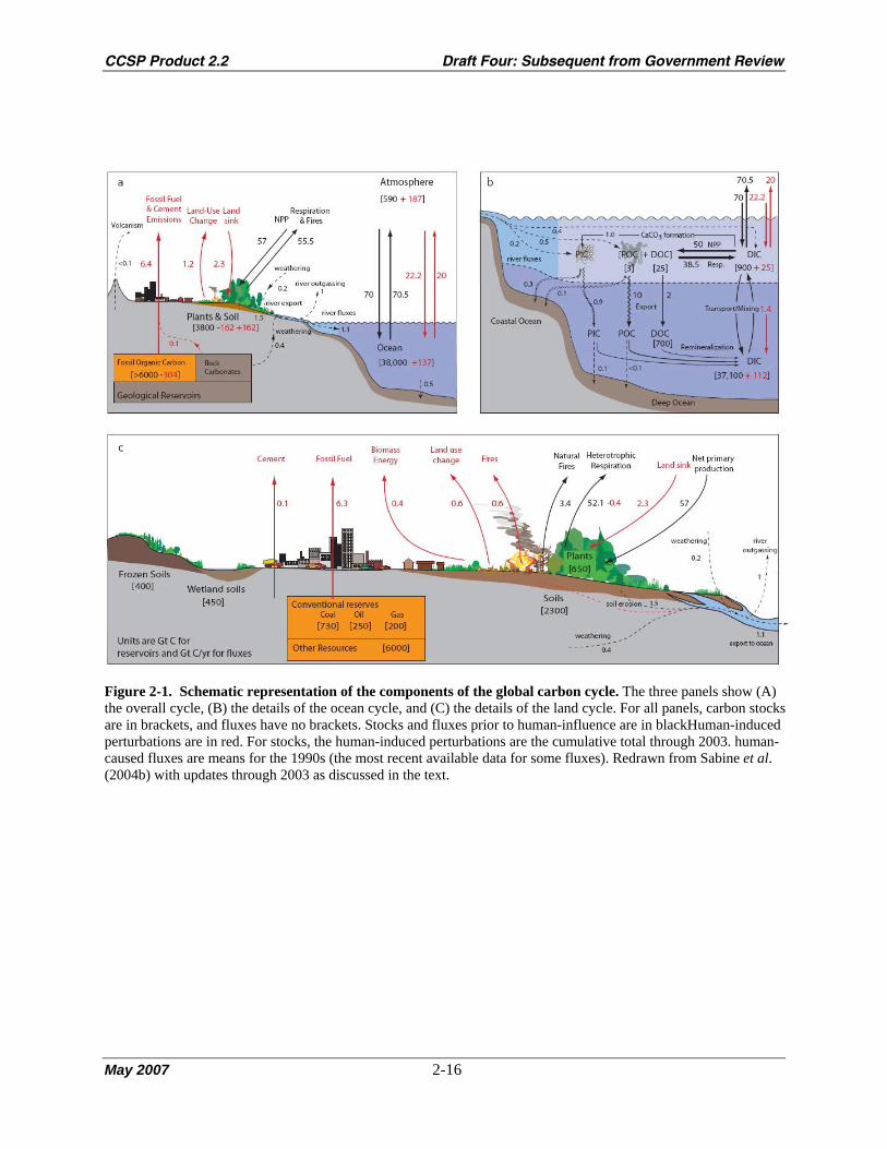
CCSP Product 2.2 Draft Four: Subsequent from Government Review
May 2007 2-16
Figure 2-1. Schematic representation of the components of the global carbon cycle. The three panels show (A) the overall cycle, (B) the details of the ocean cycle, and (C) the details of the land cycle. For all panels, carbon stocks are in brackets, and fluxes have no brackets. Stocks and fluxes prior to human-influence are in blackHuman-induced perturbations are in red. For stocks, the human-induced perturbations are the cumulative total through 2003. human-caused fluxes are means for the 1990s (the most recent available data for some fluxes). Redrawn from Sabine et al. (2004b) with updates through 2003 as discussed in the text.

CCSP Product 2.2 Draft Four: Subsequent from Government Review
May 2007 2-17
Fig. 2-2. Atmospheric CO2 concentration from 1750 to 2005. The data prior to 1957 (red circles) are from the Siple ice core (Friedli et al., 1986). The data since 1957 (blue circles) are from continuous atmospheric sampling at the Mauna Loa Observatory (Hawaii) (Keeling et al., 1976; Thoning et al., 1989) (with updates available at http://cdiac.ornl.gov/trends/co2/sio-mlo.htm).

CCSP Product 2.2 Draft Four: Subsequent from Government Review
May 2007 2-18
Figure 2-3. The 13-model mean CO2 flux interannual variability (Gt C per year) for several continents (solid lines) and ocean basins (dashed lines). In each panel, the dark inner band is the 1σ intermodel spread, the lighter adjacent band is the 1σ estimation uncertainty on interannual variability, and the outer band (visible only for the land) is the root sum of squares of the two uncertainty components. (A) North Pacific and North America, (B) Atlantic north of 15ºN and Eurasia, (C) Australasia and Tropical Pacific, (D) Africa, and (E) South America (note the different scales for Africa and South America) (Baker et al., 2006).

CCSP Product 2.2 Draft Four: Subsequent from Government Review
May 2007 3-1
Chapter 3. The North American Carbon Budget
Past and Present
Coordinating Lead Author: Stephen Pacala1
Lead Authors: Richard Birdsey,2 Scott Bridgham,3 Richard T. Conant,4 Kenneth Davis,5
Burke Hales,6 R.A. Houghton,7 J. C. Jenkins,8 Mark Johnston,9 Gregg Marland,10
and Keith Paustian4
Contributing Authors: John Caspersen,11 Robert Socolow,12 and Richard S. J. Tol13
1Department of Ecology and Evolutionary Biology, Princeton University, 2USDA Forest Service, 3Center for Ecology and Evolutionary Biology, University of Oregon, 4Natural Resource Ecology Laboratory,
Colorado State University, 5Department of Meteorology, The Pennsylvania State University, 6College of Oceanic
and Atmospheric Sciences, Oregon State University, 7Woods Hole Research Center, 8The Rubenstein School of
Environment and Natural Resources, Gund Institute for Ecological Economics, University of Vermont, 9Saskatchewan Research Council, 10Department of Engineering, Physics and Mathematics, Mid Sweden University, 11Faculty of Forestry, University of Toronto, 12Department of Mechanical and Aerospace Engineering and Princeton
Environmental Institute, Princeton University, 13Research Unit Sustainability and Global Change, Hamburg
University
KEY FINDINGS
• Fossil-fuel carbon emissions in the United States, Canada, and Mexico totaled 1856 million tons per
year in 2003 (plus or minus 10%, see Table 3-1). This represents 27% of global fossil-fuel emissions.
• Approximately 30% of North American fossil-fuel emissions are offset by a natural sink of 526 million
tons of carbon per year (plus or minus 50%) caused by a variety of factors, including forest regrowth,
wildfire suppression, and agricultural soil conservation.
• North America emits a net amount of 1330 million tons of carbon per year (plus or minus 25%) to the
atmosphere.
• North American carbon dioxide emissions from fossil fuel have increased at an average rate of
approximately 1% per year for the last 30 years.
• Growth in emissions accompanies the historical growth in the industrial economy and Gross
Domestic Product (GDP) of North America. However, at least in the United States and Canada the
rate of emissions growth is less than the growth in GDP, reflecting a decrease in the carbon intensity
of these economies.

CCSP Product 2.2 Draft Four: Subsequent from Government Review
May 2007 3-2
• Historically the plants and soils of the United States and Canada were sources for atmospheric
carbon dioxide, primarily as a consequence of the expansion of croplands into forests and
grasslands. In recent decades these regions have shifted from source to sink as forests recover from
agricultural abandonment, fire suppression is practiced, and logging is reduced, and, as a result,
these regions are now accumulating carbon. In Mexico, emissions of carbon continue to increase due
to net deforestation.
• Fossil-fuel emissions from North America are expected to continue to grow, but more slowly than
GDP.
• The future of the North American carbon sink is highly uncertain. The contribution of recovering
forests to this sink is likely to decline as these forests mature, but we do not know how much of the
sink is due to fertilization of the ecosystems by nitrogen in air pollution and by increasing carbon
dioxide concentrations in the atmosphere, nor do we understand the impact of ozone in the lower
atmosphere or how the sink will change as the climate changes. Increases in decomposition and
wildfire caused by climate change could, in principle, convert the sink into a source.
• The current magnitude of the North American sink offers the possibility that significant mitigation of
fossil-fuel emissions could be accomplished by managing forests, rangelands, and croplands to
increase the carbon stored in them. However, the range of uncertainty in these estimates is at least
as large as the estimated values themselves.
• Current trends towards lower carbon intensity of U.S. and Canadian economies increase the
likelihood that a portfolio of carbon management technologies will be able to reduce the 1% annual
growth in fossil-fuel emissions. This same portfolio might be insufficient if carbon emissions were to
begin rising at the approximately 3% growth rate of GDP.
1. FOSSIL FUEL
Fossil-fuel carbon emissions in the United States, Canada, and Mexico totaled 1856 million tons of
carbon (Mt C) per year in 2003 and have increased at an average rate of approximately 1% per year for
the last 30 years (United States = 1582, Canada = 164, Mexico = 110 Mt C per year, see Fig. 3-1).† This
represents 27% of global emissions, from a continent with 7% of the global population, and 25% of
global Gross Domestic Product (GDP) (EIA, 2005).
Figure 3-1. Historical carbon emissions from fossil fuel in the United States, Canada, and Mexico.
The United States is the world’s largest emitter in absolute terms. Its per capita emissions of 5.4 t C
per year are among the largest in the world, but the carbon intensity of its economy (emissions per unit
† Uncertainty estimates for the numerical data presented in this chapter can be found in Tables 3-1 through 3-3.
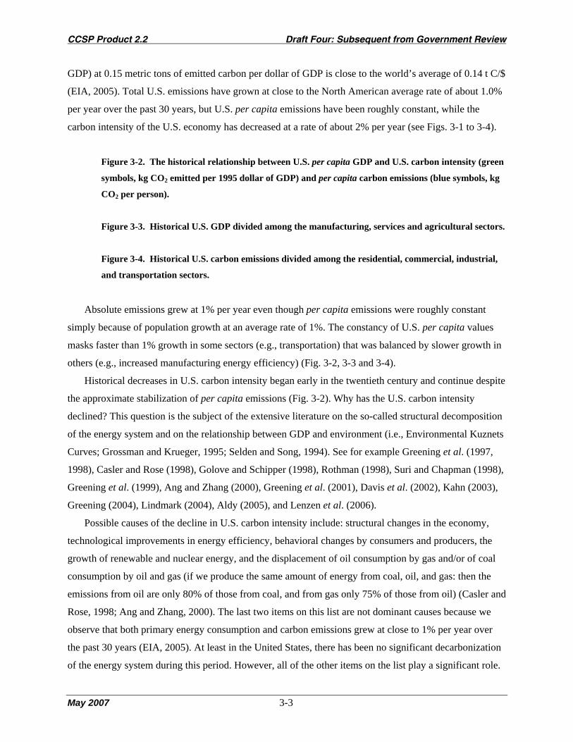
CCSP Product 2.2 Draft Four: Subsequent from Government Review
May 2007 3-3
GDP) at 0.15 metric tons of emitted carbon per dollar of GDP is close to the world’s average of 0.14 t C/$
(EIA, 2005). Total U.S. emissions have grown at close to the North American average rate of about 1.0%
per year over the past 30 years, but U.S. per capita emissions have been roughly constant, while the
carbon intensity of the U.S. economy has decreased at a rate of about 2% per year (see Figs. 3-1 to 3-4).
Figure 3-2. The historical relationship between U.S. per capita GDP and U.S. carbon intensity (green
symbols, kg CO2 emitted per 1995 dollar of GDP) and per capita carbon emissions (blue symbols, kg
CO2 per person).
Figure 3-3. Historical U.S. GDP divided among the manufacturing, services and agricultural sectors.
Figure 3-4. Historical U.S. carbon emissions divided among the residential, commercial, industrial,
and transportation sectors.
Absolute emissions grew at 1% per year even though per capita emissions were roughly constant
simply because of population growth at an average rate of 1%. The constancy of U.S. per capita values
masks faster than 1% growth in some sectors (e.g., transportation) that was balanced by slower growth in
others (e.g., increased manufacturing energy efficiency) (Fig. 3-2, 3-3 and 3-4).
Historical decreases in U.S. carbon intensity began early in the twentieth century and continue despite
the approximate stabilization of per capita emissions (Fig. 3-2). Why has the U.S. carbon intensity
declined? This question is the subject of the extensive literature on the so-called structural decomposition
of the energy system and on the relationship between GDP and environment (i.e., Environmental Kuznets
Curves; Grossman and Krueger, 1995; Selden and Song, 1994). See for example Greening et al. (1997,
1998), Casler and Rose (1998), Golove and Schipper (1998), Rothman (1998), Suri and Chapman (1998),
Greening et al. (1999), Ang and Zhang (2000), Greening et al. (2001), Davis et al. (2002), Kahn (2003),
Greening (2004), Lindmark (2004), Aldy (2005), and Lenzen et al. (2006).
Possible causes of the decline in U.S. carbon intensity include: structural changes in the economy,
technological improvements in energy efficiency, behavioral changes by consumers and producers, the
growth of renewable and nuclear energy, and the displacement of oil consumption by gas and/or of coal
consumption by oil and gas (if we produce the same amount of energy from coal, oil, and gas: then the
emissions from oil are only 80% of those from coal, and from gas only 75% of those from oil) (Casler and
Rose, 1998; Ang and Zhang, 2000). The last two items on this list are not dominant causes because we
observe that both primary energy consumption and carbon emissions grew at close to 1% per year over
the past 30 years (EIA, 2005). At least in the United States, there has been no significant decarbonization
of the energy system during this period. However, all of the other items on the list play a significant role.

CCSP Product 2.2 Draft Four: Subsequent from Government Review
May 2007 3-4
The economy has grown at an annual rate of 2.8% over the last three decades because of 3.6% growth in
the service sector; manufacturing grew at only 1.5% per year (Fig. 3-3). Because the service sector has
much lower carbon intensity than manufacturing, this faster growth of services reduces the country’s
carbon intensity. If all of the growth in the service sector had been in manufacturing from 1971 to 2001,
then the emissions would have grown at 2% per year instead of 1% (here we equate the manufacturing
sector in Fig. 3-3 with the industrial sector in Fig. 3-4). So, structural change is at least one-half of the
answer. Because the service sector is likely to continue to grow more rapidly than other sectors of the
economy, we expect that carbon emissions will continue to grow more slowly than GDP. This is
important because it implies considerable elasticity in the relationship between emissions growth and
economic growth. It also widens the range of policy options that are now technologically possible. For
example, a portfolio of current technologies able to convert the 1% annual growth in emissions into a 1%
annual decline, might be insufficient if carbon emissions were to begin rising at the ~3% growth rate of
GDP (Pacala and Socolow, 2004).
However, note that industrial emissions are approximately constant (Fig. 3-4) despite 1.5% economic
growth in manufacturing (Fig. 3-3). This decrease in carbon intensity is caused both by within-sector
structural shifts (i.e., from heavy to light manufacturing) and by technological improvements (See Part II
of this report). Emissions from the residential sector are growing at roughly the same rate as the
population (Fig. 3-4; 30-year average of 1.0% per year), while emissions from transportation are growing
faster than the population but slower than GDP (Fig. 3-4; 30-year average of 1.4% per year). The
difference between the 3% growth rate of GDP and the 1.6% growth in emissions from transportation is
not primarily due to technological improvement because carbon emissions per mile traveled have been
level or increasing over the period (Chapter 7 this report).
2. CARBON SINKS (see Tables 3-1and 3-2 for estimates, citations, and
uncertainty of estimates)
Approximately 30% of North American fossil-fuel emissions are offset by a natural sink of 526 Mt C
per year caused by a variety of factors, including forest regrowth, fire suppression, and agricultural soil
conservation. The sink currently absorbs 492 Mt C per year in the United States and 83 Mt C per year in
Canada. Mexican ecosystems create a net source of 48 Mt C per year. Rivers and international trade also
export a net of 161 Mt C per year that was captured from the atmosphere by the continent’s ecosystems,
and so North America absorbs 687 Mt C per year of atmospheric CO2 (687 = 526 + 161). Because most
of these net exports will return to the atmosphere elsewhere within 1 year (e.g. carbon in exported grain
will be eaten, metabolized, and exhaled as CO2), the net North American sink is rightly thought of as 526
Mt C per year even though the continent absorbs a net of 687 Mt C per year. Moreover, coastal waters

CCSP Product 2.2 Draft Four: Subsequent from Government Review
May 2007 3-5
may be small net emitters to the atmosphere at the continental scale (19 Mt C per year), but this flux is
highly uncertain (see Chapter 15 this report). The portion of the coastal flux caused by human activity is
thought to be close to zero, so coastal sea-air exchanges should be excluded from the continental carbon
sink.
As reported in Chapter 2, the sink in the United States is approximately 40% (plus or minus 20%) the
size of the global carbon sink, while the sink in Canada is about 7% (plus or minus 7%) the size of the
global sink. The source in Mexico reduces the global sink by ~4% (plus or minus more than 4%). The
reason for the disproportionate importance of U.S. sinks is probably the unique land use history of the
country (summary in Appendix 3A). During European settlement, large amounts of carbon were released
from the harvest of virgin forests and the plowing of virgin soils to create agricultural lands. The
abandonment of many of the formerly agricultural lands in the east and the regrowth of forest is a unique
event globally and is responsible for about one-half of the U.S. sink (Houghton et al., 2000). Most of the
U.S. sink thus represents a one-time recapture of some of the carbon that was released to the atmosphere
during settlement. In contrast, Mexican ecosystems, like those of many tropical nations, are still a net
carbon source because of ongoing deforestation (Masera et al., 1997).
Table 3-1. Annual net carbon emissions (source = positive) or uptake (land sink = negative) of
carbon in millions of tons.
Table 3-2. Annual net horizontal transfers of carbon in millions of tons.
Table 3-3. Carbon stocks in North America in billions of tons.
The non-fossil fluxes in Tables 3-1 and 3-2, are derived exclusively from inventory methods in which
the total amount of carbon in a pool (i.e., living forest trees plus forest soils) is measured on two
occasions. The difference between the two measurements shows if the pool is gaining (sink) or losing
(source) carbon. Carbon inventories are straightforward in principle, but of uneven quality in practice. For
example, we know the carbon in living trees in the United States relatively accurately because the U.S.
Forest Service Forest Inventory program measures trees systematically in more than 200,000 locations.
However, we must extrapolate from a few measurements of forest soils with models because there is no
national inventory of carbon in forest soils.
Although the fluxes in Tables 3-1 and 3-2 represent the most recent published estimates, with most
less than five years old, a few are older than ten years (see the citations at the bottom of each Table).
Also, the time interval between inventories varies among the elements of the Tables, with most covering a
five to ten year period. In these tables and throughout this document we report uncertainties using six

CCSP Product 2.2 Draft Four: Subsequent from Government Review
May 2007 3-6
categories: ***** = 95% certain that the actual value is within 10% of the estimate reported, **** = 95%
certain that the estimate is within 25%, *** = 95% certain that the estimate is within 50%, ** = 95%
certain that the estimate is within 100%, * = uncertainty greater than 100%.
In addition to inventory methods, it is also possible to estimate carbon sources and sinks by
measuring carbon dioxide (CO2) in the atmosphere. For example, if air exits the border of a continent
with more CO2 than it contained when it entered, then there must be a net source of CO2 somewhere
inside the continent. We do not include estimates obtained in this way because they are still highly
uncertain at continental scales. Pacala et al. (2001) found that atmosphere- and inventory-based methods
gave consistent estimates of U.S. ecosystem sources and sinks but that the range of uncertainty from the
former was considerably larger than the range from the latter. For example, by far the largest published
estimate for the North American carbon sink was produced by an analysis of atmospheric data by Fan et
al. (1998) (-1700 Mt C per year). The appropriate inventory-based estimate to compare this to is our -687
Mt C per year of net absorption (atmospheric estimates include net horizontal exports by rivers and trade),
and this number is well within the wide uncertainty limits in Fan et al. (1998). The allure of estimates
from atmospheric data is that they do not risk missing critical uninventoried carbon pools. But, in
practice, they are still far less accurate at continental scales than a careful inventory (Pacala et al., 2001).
Using today's technology, it should be possible to complete a comprehensive inventory of the sink at
national scales, with the same accuracy as the U.S. forest inventory currently achieves for above-ground
carbon in forests (25%, Smith and Heath, 2005). Moreover, this inventory would provide disaggregated
information about the sink’s causes and geographic distribution. In contrast, estimates from atmospheric
methods rely on the accuracy of atmospheric models, and estimates obtained from different models vary
by 100% or more at the scale of the United States, Canada, or Mexico (Gurney et al., 2004). Nonetheless,
extensions of the atmospheric sampling network should improve the accuracy of atmospheric methods
and might allow them to achieve the accuracy of inventories at regional and whole-country scales. In
addition, atmospheric methods will continue to provide an independent check on inventories to make sure
that no large flux is missed, and atmospheric methods will remain the only viable method to assess
interannual variation the continental flux of carbon.
The current magnitude of the North American sink documented in Tables 3-1 and 3-2 offers the
possibility that significant carbon mitigation could be accomplished by managing forests, rangelands, and
croplands to increase the carbon stored in them. However, many of the estimates in Tables 3-1 and 3-2 are
highly uncertain; for some the range of uncertainty is larger than the value reported. The largest
contributors to the uncertainty in the U.S. sink are the amount of carbon stored on rangelands because of
the encroachment of woody vegetation and the lack of comprehensive and continuous inventory of
Alaskan lands. A carbon inventory of these lands would do more to constrain the size of the U.S. sink

CCSP Product 2.2 Draft Four: Subsequent from Government Review
May 2007 3-7
than would any other measurement program of similar cost. Also we still lack comprehensive U.S.
inventories of carbon in soils, woody debris, wetlands, rivers, and reservoirs. Finally, we lack estimates of
any kind for five significant components of the carbon budget in Canada and six in Mexico (see Table 3-1
and 3-2).
The cause and future of the North American carbon sink is also highly uncertain. Although we can
document the accumulation of carbon in ecosystems and wood products, we do not know how much of
the sink is due to fertilization of the ecosystems by the nitrogen in air pollution and by the added CO2 in
the atmosphere, we do not fully understand the impact of tropospheric ozone, nor do we understand
precisely how the sink will change as the climate changes. Research is mixed about the importance of
nitrogen and CO2 fertilization (Casperson et al., 2000; Oren et al., 2001; Hungate et al., 2003; Luo 2006;
Körner et al., 2005). If these factors are weak, then, all else equal, we expect the North American sink to
decline over time as ecosystems complete their recovery from past exploitation (Hurtt et al., 2002).
However, if these factors are strong, then the sink could grow in the future. Similarly, global warming is
expected to lengthen the growing season in most parts of North America, which should increase the sink
(but see Goetz et al., 2005). But warming is also expected to increase forest fire and the rate of
decomposition of dead organic matter, which should decrease the sink and might convert it into a source
(Gillett et al., 2004; Flannigan et al., 2005; Schaphoff et al., 2006; Westerling et al., 2006). The relative
strength of the various opposing factors is still difficult to predict. Experimental manipulations of climate,
atmospheric CO2, tropospheric ozone, and nitrogen, at the largest possible scale, will be required to
reduce uncertainty about the future of the carbon sink.
In what follows, we provide additional detail about the elements in Tables 3-1 and 3-2.
2.1 Forests
Based on U.S. Forest Service inventories, forest ecosystem carbon stocks in the United States,
excluding soil carbon, have increased since 1953. The rate of increase has recently slowed because of
increasing harvest and declining growth in some areas with maturing forests. The current average annual
increase in carbon in trees is 146 Mt C per year (Smith and Heath, 2005, uncertainty ****) plus 23 Mt C
per year from urban and suburban trees (the midpoint of the range in Chapter 14, uncertainty ***). The
total estimate of the carbon sink in forested ecosystems is -259 Mt C per year and includes a sink of 90
Mt C per year (uncertainty **) from the accumulation of nonliving carbon in the soil (-90-146-23 = -259)
(Pacala et al., 2001; Goodale et al., 2002). Although the magnitude of the forest soil sink has always been
uncertain, it is now possible to measure the total above-and below-ground sink in a few square kilometers
by monitoring the atmospheric CO2 that flows into and out of the site over the course of a year. Note that
these spatially intensive methods, appropriate for monitoring the sink over a few square kilometers, are

CCSP Product 2.2 Draft Four: Subsequent from Government Review
May 2007 3-8
unrelated to the spatially extensive methods described above, which attempt to constrain the sink at
continental scales. As described in Appendix 3B, these studies are producing data that so far confirm the
estimates of inventories and show that most of the forest sink is above ground.
According to Canada’s Greenhouse Gas Inventory (Environment Canada 2005, Chapter 11 this
report), managed forests in Canada (comprising 82% of the total forest area) sequestered 17 Mt C above
ground in 1990 (uncertainty **). In addition, Goodale et al. (2002) estimate the sink of nonliving carbon
belowground to be -30 Mt C per year for the period 1990-1994 (uncertainty **).
The two published carbon inventories for Mexican forests (Masera et al., 1997 and Cairns et al.,
2000) both report substantial losses of forest carbon, primarily because of deforestation in the tropical
south. However, both of these studies rely on calculations of carbon loss from remote imagery, rather than
direct measurements, and both report results for a period that ended more than 10 years ago. Thus, in
addition to being highly uncertain, the estimates for Mexican forests in Table 3-1 are not recent.
2.2 Wood Products
Wood products create a carbon sink because they accumulate both in use (e.g., furniture, house
frames, etc.) and in landfills. The wood products sink is estimated at -57 Mt C per year in the United
States (Skog and Nicholson, 1998) and -11 Mt C per year in Canada (Goodale et al., 2002, Chapter 11
this report). We know of no estimates for Mexico.
2.3 Woody Encroachment
Woody encroachment is the invasion of woody plants into grasslands or the invasion of trees into
shrublands. It is caused by a combination of fire suppression and grazing. Fire inside the United States
has been reduced by more than 95% from the pre-settlement level of approximately 80 million hectares
burned per year, and this favors shrubs and trees in competition with grasses (Houghton et al., 2000).
Field studies show that woody encroachment both increases the amount of living plant carbon and
decreases the amount of dead carbon in the soil (Guo and Gifford, 2002; Jackson et al., 2002). Although
the total gains and losses are ultimately of similar magnitude (Jackson et al., 2002), the losses occur
within approximately a decade after the woody plants invade (Guo and Gifford, 2002), while the gains
occur over a period of up to a century or more. Thus, the net source or sink depends on the distribution of
times since woody plants invaded, and this is not known. Estimates for the size of the current U.S. woody
encroachment sink (Kulshreshtha et al., 2000; Houghton and Hackler, 2000; and Hurtt et al., 2002) all
rely on methods that do not account for the initial rapid loss of carbon from soil when grasslands were
converted to shrublands or forest. The estimate of -120 Mt C per year in Table 3-1 is from Kulshreshtha et
al. (2000) but is similar to the estimates from the other two studies (-120 and -130 Mt C per year). No
CCSP Product 2.2 Draft Four: Subsequent from Government Review
May 2007 3-9
estimates are currently available for Canada or Mexico. Note the error estimate of more than 100% in
Table 3-1. A comprehensive set of measurements of woody encroachment would reduce the error in the
national and continental carbon budgets more than any other inventory.
2.4 Agricultural Lands
Soils in croplands and grazing lands have been historically depleted of carbon by humans and their
animals, especially if the land was converted from forest to non-forest use. Harvest or consumption by
animals reduces the input of organic matter to the soil, while tillage and manure inputs increase the rate of
decomposition. Changes in cropland management, such as the adoption of no-till agriculture (see Chapter
10 this report), have reversed the losses of carbon on some croplands, but the losses continue on the
remaining lands. The net is a small sink of -2 Mt C per year for agricultural soils in Canada and for the
United States is a sink of between -5 and -12 Mt C per year.
2.5 Wetlands
Peatlands are wetlands that have accumulated deep soil carbon deposits because plant productivity
has exceeded decomposition over thousands of years. Thus, wetlands form the largest carbon pool of any
North American ecosystem (Table 3-3). If drained for development, this soil carbon pool is rapidly lost.
Canada’s extensive frozen and unfrozen wetlands create a net sink of -23 and Mt C per year (see Chapters
12 and 13 this report), but drainage of peatlands in the United States has created a net source of 6 Mt C
per year. The very large pool of peat in northern wetlands is vulnerable to climate change and could add
more than 100 ppm to the atmosphere (1 ppm ≈ 2.1 billion tons of carbon [Gt C]) during this century if
released because of global warming (see the model result in Cox et al., 2000 for an example).
The carbon sink due to sedimentation in wetlands is estimated to be 4 Mt C per year in Canada and 27
Mt C per year in the United States but this estimate is highly uncertain (see Chapter 13 this report).
Another important priority for research is to better constrain carbon sequestration due to sedimentation in
wetlands, lakes, reservoirs, and rivers.
The focus on this chapter is on CO2; we do not include estimates for other greenhouse gases.
However, wetlands are naturally an important source of methane (CH4). Methane emissions effectively
cancel out the positive benefits of any carbon storage as peat in Canada and make U.S. wetlands a source
of warming on a decadal time scale (Chapter 13 this report). Moreover, if wetlands become warmer and
remain wet with future climate change, they have the potential to emit large amounts of CH4. This is
probably the single most important consideration, and unknown, in the role of wetlands and future climate
change.

CCSP Product 2.2 Draft Four: Subsequent from Government Review
May 2007 3-10
2.6 Rivers and Reservoirs
Organic sediments accumulate in artificial lakes and in alluvium (deposited by streams and rivers),
and colluvium (deposited by wind or gravity) and represent a carbon sink. Pacala et al. (2001) extended
an analysis of reservoir sedimentation (Stallard, 1998) to an inventory of the 68,000 reservoirs in the
United States and also estimated net carbon burial in alluvium and colluvium. Table 3-1 includes the
midpoint of their estimated range of 10 to 40 Mt C per year in the coterminous United States. This
analysis has also recently been repeated and produced an estimate of 17 Mt C per year (E. Sundquist,
personal communication; unreferenced). We know of no similar analysis for Canada or Mexico.
2.7 Exports Minus Imports of Wood and Agricultural Products
The United States imports more wood products (14 Mt C per year) than it exports and exports more
agricultural products (35 Mt C per year) than it imports (Pacala et al., 2001). The large imbalance in
agricultural products is primarily because of exported grains and oil seeds. Canada and Mexico are net
wood exporters, with Canada at -74 Mt C per year (Environment Canada, 2005) and Mexico at -1 Mt C
per year (Masera et al., 1997). The North American export of 61 Mt C per year accounts correctly for the
large net transfer of lumber and wood products from Canada to the United States. We know of no analysis
of the Canadian or Mexican export-import balance for agricultural products.
2.8 River Export
Rivers in the coterminous United States were estimated to export 30-40 Mt C per year to the oceans
in the form of dissolved and particulate organic carbon and inorganic carbon derived from the atmosphere
(Pacala et al., 2001). An additional 12-20 Mt C per year of inorganic carbon is also exported by rivers but
is derived from carbonate minerals. We know of no corresponding estimates for Alaska, Canada, or
Mexico.
2.9 Coastal Waters
Chapter 15 summarizes the complexity and large uncertainty of the sea-air flux of CO2 in North
American coastal waters. It is important to understand that the source in Mexican coastal waters is not
caused by humans and would have been present in pre-industrial times. It is simply the result of the
purely physical upwelling of carbon-rich deep waters and is a natural part of the oceanic carbon cycle. It
is not yet known how much of the absorption of carbon by U.S. and Canadian coastal waters is natural
and how much is caused by nutrient additions to the coastal zone by humans. Accordingly, it is essentially

CCSP Product 2.2 Draft Four: Subsequent from Government Review
May 2007 3-11
impossible to currently assess the potential or costs for carbon management in coastal waters of North
America.
3. SUMMARY
Fossil-fuel emissions currently dominate the net carbon balance in the United States, Canada, and
Mexico (Fig. 3-1, Tables 3-1, 3-2). Fossil-fuel consumption in the United States currently emits 1582 Mt
C per year to the atmosphere (confidence ****, see definition of confidence categories in Table 3-1
footnote). This is partially balanced by a flow of 492 Mt C per year from the atmosphere to land caused
by net ecosystem sinks in the United States (***). Canadian fossil-fuel consumption transfers 164 Mt C
per year to the atmosphere (****), but net ecological sinks capture 83 Mt C per year (**). Mexican fossil-
fuel emissions of 110 Mt C per year (****) are supplemented by a net ecosystem source of 48 Mt C per
year (*) from tropical deforestation. Each of the three countries has always been a net source of CO2
emissions to the atmosphere for the past three centuries (Houghton et al., 1999, 2000; Houghton and
Hackler, 2000; Hurtt et al., 2002).
CHAPTER 3 REFERENCES
Aldy, J.E., 2005: An environmental kuznets curve analysis of US state level carbon dioxide emissions. Journal of
Environment and Development, 14(1), 58-72.
Ang, B.W. and F.Q. Zhang, 2000: A survey of index decomposition analysis in energy and environmental studies.
Energy, 25, 1149-1176.
Bradley, B.A., R.A. Houghton, J.F. Mustard, and S.P. Hamburg, 2006: Invasive grass reduces carbon stocks in
shrublands of the Western U.S. (in press).
Cairns, M.A., P.K. Haggerty, R. Alvarez, B.H.J. De Jong, and I. Olmsted, 2000: Tropical Mexico’s recent land-use
change: a region’s contribution to the global carbon cycle. Ecological Applications, 10(5), 1426-1441.
Casler, S.D. and A.Z. Rose, 1998: Carbon dioxide emissions in the US economy. Environmental and Resource
Economics, 11(3-4), 349-363.
Caspersen, J.P., S.W. Pacala, J.C. Jenkins, G.C. Hurtt, P.R. Moorcroft, and R.A. Birdsey, 2000: Contributions of
land-use history to carbon accumulation in U.S. forests. Science, 290, 1148-1151.
Cox, P.M., R.A. Betts, C.D. Jones, S.A. Spall, and I.J. Totterdell, 2000: Acceleration of global warming due to
carbon-cycle feedbacks in a coupled climate model. Nature, 408, 184-187.
Davis, W.B., A.H. Sanstad, and J.G. Koomey, 2002: Contributions of weather and fuel mix to recent declines in US
energy and carbon intensity. Energy Economics, 25, 375-396.
Defries, R.S., R.A. Houghton, M.C. Hansen, C.B. Field, D. Skole, and J. Townshend, 2002: Carbon emissions from
tropical deforestation and regrowth based on satellite observations for the 1980s and 1990s. Proceedings of the
National Academy of Sciences of the United States of America, 99(22), 14256-14261.

CCSP Product 2.2 Draft Four: Subsequent from Government Review
May 2007 3-12
EIA (Energy Information Administration), 2005: Historical Data Overview. U.S. Department of Energy. Available
at http://www.eia.doe.gov/overview_hd.html; http://cdiac.ornl.gov/ftp/trends/emis/meth-reg.htm
Environment Canada, 2005: Canada’s Greenhouse Gas Inventory 1990-2003: Initial Submission. Greenhouse Gas
Division, Environment Canada, Ottawa, Ontario, Canada. Available at
http://unfccc.int/national_reports/annex_i_ghg_inventories/national_inventories_submissions/items/2761.php
Fan, S.-M., M. Gloor, J. Mahlman, S. Pacala, J. Sarmiento, T. Takahashi, and P. Tans, 1998: Atmospheric and
oceanic CO2 data and models imply a large terrestrial carbon sink in North America. Science, 282, 442-446.
Flannigan, M.D., K.A. Logan, B.D. Amiro, W.R. Skinner, and B.J. Stocks. 2005: Future area burned in Canada.
Climatic Change, 72, 1-16.
Gillett, N.P., A.J. Weaver, F.W. Zwiers, and M.D. Flannigan, 2004: Detecting the effect of climate change on
Canadian forest fires. Geophysical Research Letters, 31; L18211. doi:10.1029/2004GL020876
Goetz, S.J., A. Bunn, G. Fiske, and R.A. Houghton. 2005: Satellite observed photosynthetic trends across boreal
North America associated with climate and fire disturbance. Proceedings National Academy of Science
102:13521-13525.
Golove, W.H. and L.J. Schipper, 1998: Long-term trends in us manufacturing energy consumption and carbon
dioxide emissions. Energy, 21(7/8), 683-692.
Goodale, C.L., M.J. Apps, R.A. Birdsey, C.B. Field, L.S. Heath, R.A. Houghton, J.C. Jenkins, G.H. Kohlmaier, W.
Kurz, S. Liu, G.J. Nabuurs, S. Nilsson, and A.Z. Shvidenko, 2002: Forest carbon sinks in the northern
hemisphere. Ecological Applications, 12(3), 891-899.
Greening, L.A., W.B. Davis, L. Schipper, and M. Khrushch, 1997: Comparison of six decomposition methods:
application to aggregate energy intensity for manufacturing in 10 OECD countries. Energy Economics, 19(3),
375-390.
Greening, L.A., W.B. Davis, and L. Schipper, 1998: Decomposition of aggregate carbon intensity for the
manufacturing sector: comparison of declining trends from 10 OECD countries for the period 1971-1993.
Energy Economics, 20(1), 43-65.
Greening, L.A., M. Ting, and W.B. Davis, 1999: Decomposition of aggregate carbon intensity for freight: trends
from 10 OECD countries for the period 1971-1993. Energy Economics, 21(4), 331-361.
Greening, L.A., M. Ting, and T.J. Krackler, 2001: Effects of changes in residential end-uses on aggregate carbon
intensity: comparison of 10 OECD countries for the period 1970 through 1993. Energy Economics, 23(2), 153-
178.
Greening, L.A., 2004: Effects of human behavior on aggregate carbon intensity of personal transportation:
comparison of 10 OECD countries for the period 1970-1993. Energy Economics, 26(1), 1-30.
Grossman, G.M. and A.B. Krueger, 1995: Economic growth and the environment. Quarterly Journal of Economics,
60(2), 353-375.
Guo, L.B. and R.M. Gifford, 2002: Soil carbon stocks and land use change: a meta analysis. Global Change
Biology, 8(4), 345-360.

CCSP Product 2.2 Draft Four: Subsequent from Government Review
May 2007 3-13
Gurney, K.R., R.M. Law, A.S. Denning, P.J. Rayner, B.C. Pak, D. Baker, P. Bousquet, L. Bruhwiler, Y.H. Chen, P.
Ciais, I.Y. Fung, M. Heimann, J. John, T. Maki, S. Maksyutov, P. Peylin, M. Prather, and S. Taguchi, 2004:
Transcom 3 inversion intercomparison: model mean results for the estimation of seasonal carbon sources and
sinks. Global Biogeochemical Cycles, 18, GB1010.
Houghton, R.A., J.L. Hackler, and K.T. Lawrence, 1999: The U.S. carbon budget: contributions from land-use
change. Science, 285, 574-578.
Houghton, R.A. and J.L. Hackler, 2000: Changes in terrestrial carbon storage in the United States. 1. The roles of
agriculture and forestry. Global Ecology and Biogeography, 9, 125-144.
Houghton, R.A., J.L. Hackler, and K.T. Lawrence, 2000: Changes in terrestrial carbon storage in the United States.
2. The role of fire and fire management. Global Ecology and Biogeography, 9, 145-170.
Hungate, B.A., J.S. Dukes, M.R. Shaw, Y. Luo, and C.B. Field, 2003: Nitrogen and climate change. Science, 302,
1512-1513.
Hurtt, G.C., S.W. Pacala, P.R. Moorcroft, J. Caspersen, E. Shevliakova, R.A. Houghton, and B. Moore III, 2002:
Projecting the future of the U.S. carbon sink. Proceedings of the National Academy of Sciences of the United
States of America, 99, 1389-1394.
Jackson, R.B., J.L. Banner, E.G. Jobbagy, W.T. Pockman, and D.H. Wall, 2002: Ecosystem carbon loss with
woody plant invasion of grasslands. Nature, 418(6898), 623-626.
Kahn, M.E., 2003: The geography of US pollution intensive trade: evidence from 1958 to 1994. Regional Science
and Urban Economics, 33, 383-400.
Körner, C., R. Asshoff, O. Bignucolo, S. Hättenschwiler, S.G. Keel, S. Peláez-Riedl, S. Pepin, R.T.W. Siegwolf,
and G. Zotz, 2005: Carbon flux and growth in mature deciduous forest trees exposed to elevated CO2. Science,
309, 1360-1362.
Kulshreshtha, S.N., B. Junkins, and R. Desjardins, 2000: Prioritizing greenhouse gas emission mitigation measures
for agriculture. Agricultural Systems, 66(3), 145-166.
Lenzen, M., M. Wier, C. Cohen, H. Hayami, S. Pachauri, and R. Schaeffer, 2006: A comparative multivariate
analysis of household energy requirements in Australia, Brazil, Denmark, India and Japan. Energy, 31, 181-207.
Lindmark, M., 2004: Patterns of historical CO2 intensity transitions among high and low income countries.
Explorations in Economic History, 41, 426-447.
Luo, Y., D. Hui, and D. Zhang, 2006: Elevated carbon dioxide stimulates net accumulations of carbon and nitrogen
in terrestrial ecosystems: a meta-analysis. Ecology (forthcoming in the 1st issue).
Masera, O.R., M.J. Ordonez, and R. Dirzo, 1997: Carbon emissions from Mexican forests: current situation and
long-term scenarios. Climate Change, 35, 265-295.
Maddison, A., 2003: The World Economy: Historical Statistics. OECD, Paris.
Marland, G., T.A. Boden, and R.J. Andres, 2005: Global, regional and national CO2 emissions. In: Trends: A
Compendium of Data on Global Change. Oak Ridge National Laboratory, Oak Ridge, TN. Available at
http://cdiac.esd.ornl.gov/trends/emis/em_cont.htm

CCSP Product 2.2 Draft Four: Subsequent from Government Review
May 2007 3-14
Mitchell, B.R., 1998: International Historical Statistics: The Americas, 1750-1993. 4th Edition, Stockton Press,
New York, NY.
Oren, R., D.S. Ellsworth, K.H. Johnsen, N. Phillips, B.E. Ewers, C. Maier, K.V.R. Schäfer, H. McCarthy,
G. Hendrey, S.G. McNulty, and G.G. Katul, 2001: Soil fertility limits carbon sequestration by forest ecosystems
in a CO2-enriched atmosphere. Nature, 411, 469-478.
Pacala, S.W., G.C. Hurtt, R.A. Houghton, R.A. Birdsey, L. Heath, E.T. Sundquist, R.F. Stallard, D. Baker,
P. Peylin, P. Moorcroft, J. Caspersen, E. Shevliakova, M.E. Harmon, S.-M. Fan, J.L. Sarmiento, C. Goodale,
C.B. Field, M. Gloor, and D. Schimel, 2001: Consistent land- and atmosphere-based U.S. carbon sink estimates.
Science, 292(5525), 2316-2320.
Pacala, S.W. and R.H. Socolow, 2004: Stabilization wedges: solving the climate problem for the next 50 years with
current technologies. Science, 305(5686), 968-972.
Rothman, D.S., 1998: Environmental Kuznets curves—real progress or passing the buck: a case for consumption-
based approaches. Ecological Economics, 25, 177-194.
Schaphoff, S., W. Lucht, D. Gerten, S. Sitch, W. Cramer, and I.C. Prentice, 2006: Terrestrial biosphere carbon
storage under alternative climate projections. Climatic Change, 74, 97-122.
Selden, T.M. and D. Song, 1994: Environmental quality and development—is there a kuznets curve for air pollution
emissions? Journal of Environmental Economics and Management, 27, 147-162.
Skog, K.E. and G.A. Nicholson, 1998: Carbon cycling through wood products: the role of wood and paper products
in carbon sequestration. Forest Products Journal, 48, 75-83. Available at
http://www.fpl.fs.fed.us/documnts/pdf1998/skog98a.pdf
Skog, K.E., K. Pingoud, and J.E. Smith, 2004: A method countries can use to estimate changes in carbon stored in
harvested wood products and the uncertainty of such estimates. Environmental Management, 33 (Supplement
1), S65-S73.
Smith, J.E. and L.S. Heath, 2005: Land use change and forestry and related sections (excerpted). In: U.S.
Environmental Protection Agency, Inventory of U.S. Greenhouse Gas Emissions and Sinks: 1990-2003. EPA
430-R-05-003. Available at http://yosemite.epa.gov/oar/globalwarming.nsf/content/
ResourceCenterPublicationsGHGEmissionsUSEmissionsInventory2005.html
Stallard, R.F., 1998: Terrestrial sedimentation and the carbon cycle: coupling weathering and erosion to carbon
burial. Global Biogeochemical Cycles, 12(2), 231.
Suri, V. and D. Chapman, 1998: Economic growth, trade and energy: implications for the environmental kuznets
curve. Ecological Economics, 25(2), 195-208.
Westerling, A., H.G. Hidalgo, D.R. Cayan, and T.W. Swetnam, 2006: Warming and earlier Spring increase western
U.S. forest wildfire activity. Science, 313, 940-943.
World Forest Institute, 2006: http://wfi.worldforestrycenter.org/trade-2.htm
WRI (World Resources Institute), 2005: EarthTrends—The Environmental Information Portal. Available at
http://earthtrends.wri.org/

CCSP Product 2.2 Draft Four: Subsequent from Government Review
May 2007 3-15
Table 3-1. Annual net emissions (source = positive) or uptake (land sink = negative)
of carbon in millions of tons
Source (positive) or Sink (negative) United States Canada Mexico North America Fossil source (positive)
Fossil fuel (oil, gas, coal) 1582a,*****
(681, 328, 573) 164a,*****
(75, 48, 40) 110a,*****
(71, 29, 11) 1856*****
(828, 405, 624) Non-fossil carbon sink (negative) or
source (positive)
Forest -259b,*** -47c,*** +52d,** -254***
Wood products -57e,*** -11 f,*** ND -68*** Woody encroachment -120g,* ND ND -120*
Agricultural soils -8h,*** -2h, *** ND -10h, ***
Wetlands -23i,* -23i,* -4i,* -49*
Rivers and reservoirs -25 j,** ND ND -25*
Total carbon source or sink -492*** -83** 48* -526***
Net carbon source (positive) 1090**** 81*** 158*** 1330****
Uncertainty:
*****(95% confidence within 10%) ****(95% confidence within 25%) ***(95% confidence within 50%) **(95% confidence within 100%) *(95% confidence bounds greater than 100%) ND = No data available ahttp://www.eia.doe.gov/env/inlenv.htm bSmith and Heath (2005) for above ground carbon, but including 23 Mt C per year for U.S. urban and suburban forests from
Chapter 14, and Pacala et al. (2001) for below ground carbon. cEnvironment Canada (2005), Chapter 11 dMasera et al. (1997) eSkog et al. (2004), Skog and Nicholson (1998) fGoodale et al. (2002) gKulshreshtha et al. (2000), Hurtt et al. (2002), Houghton and Hackler (1999). hChapter 10; Uncertain; Could range from -7 Mt C per year to -14 Mt C per year for North America. iChapter 13 jStallard, 1998; Pacala et al. (2001)

CCSP Product 2.2 Draft Four: Subsequent from Government Review
May 2007 3-16
Table 3-2. Annual net horizontal transfers of carbon in millions of tons.
Uncertainty:
*****(95% confidence within 10%) ****(95% confidence within 25%) ***(95% confidence within 50%) **(95% confidence within 100%) *(95% confidence bounds greater than 100%) ND = No data available aEnvironment Canada (2005), World Forest Institute (2006) bMasera et al. (1997) cSkog et al. (2004), Skog and Nicholson (1998) dPacala et al. (2001) eChapter 15
Net horizontal transfer: imports exceed exports = positive; exports
exceed imports = negative United States Canada Mexico North America
Wood products 14c,**** -74a,**** -1b,* -61****
Agriculture products -65d,*** ND ND -65***
Rivers to ocean -35d,** ND ND -35*
Total net absorption (Total carbon source or sink in
Table 3-1 plus exports)
-574*** -143** 47* -681**
Net absorption (negative) or emission (positive) by coastal waters
ND ND ND 19e,*
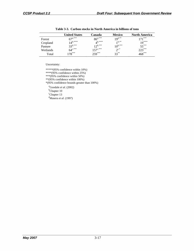
CCSP Product 2.2 Draft Four: Subsequent from Government Review
May 2007 3-17
Table 3-3. Carbon stocks in North America in billions of tons
United States Canada Mexico North America Forest 67a,*** 86a,*** 19d,** 171***
Cropland 14b,**** 4b,**** 1b,** 19****
Pasture 33b,*** 12b,*** 10b,*** 55***
Wetlands 64c,*** 157c,*** 2c,* 223***
Total 178*** 259*** 33** 468***
Uncertainty:
*****(95% confidence within 10%) ****(95% confidence within 25%) ***(95% confidence within 50%) **(95% confidence within 100%) *(95% confidence bounds greater than 100%)
aGoodale et al. (2002) bChapter 10 cChapter 13 dMasera et al. (1997)

CCSP Product 2.2 Draft Four: Subsequent from Government Review
May 2007 3-18
Fig. 3-1. Historical carbon emissions from fossil fuel in the United States, Canada, and Mexico. Data from
the U.S. Energy Information Administration (EIA 2005).

CCSP Product 2.2 Draft Four: Subsequent from Government Review
May 2007 3-19
Fig. 3-2. The historical relationship between U.S. per capita GDP and U.S. carbon intensity (green
symbols, kg CO2 emitted per 1995 dollar of GDP) and per capita carbon emissions (blue symbols, kg CO2 per
person). Each symbol shows a different year and each of the two time series progresses roughly chronologically
from left (early) to right (late) and ends in 2002. Source: Maddison (2003), Marland et al. (2005). Thus, the red
square farthest to the right shows U.S. per capita CO2 emissions in 2002. The square second farthest to the right
shows per capita emissions in 2001. The third farthest to the right shows 2000, and so on. Note that per capita
emissions have been roughly constant over the last 30 years (squares corresponding to per capita GDP greater than
approximately $16,000).

CCSP Product 2.2 Draft Four: Subsequent from Government Review
May 2007 3-20
Figure 3-3. Historical U.S. GDP divided among the manufacturing, services, and agricultural sectors.
Source: Mitchell (1998), WRI (2005).
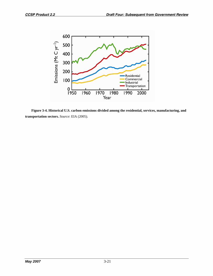
CCSP Product 2.2 Draft Four: Subsequent from Government Review
May 2007 3-21
Figure 3-4. Historical U.S. carbon emissions divided among the residential, services, manufacturing, and
transportation sectors. Source: EIA (2005).
CCSP Product 2.2 Draft Four: Subsequent from Government Review
May 2007 3-22
[This page intentionally left blank]
CCSP Product 2.2 Draft Four: Subsequent from Government Review
May 2007 4-1
Chapter 4. What Are the Options that Could Significantly Affect the North American and Global Carbon Cycles?
Coordinating Lead Author: Erik Haites1
Lead Authors: Ken Caldeira,2 Patricia Romero Lankao,3 Adam Rose,4 and Tom Wilbanks5
Contributing Authors: Skip Laitner,6 Richard Ready,7 and Roger Sedjo8
1Margaree Consultants, Inc., 2Carnegie Institution, 3Metropolitan Autonomous University—Xochimilco and
Institute for the Study of Society and Environment (NCAR), 4The Pennsylvania State University and University of
Southern California, 5Oak Ridge National Laboratory, 6U.S. Environmental Protection Agency, 7The Pennsylvania State University, 8Resources for the Future
KEY FINDINGS
• Options to reduce energy-related carbon dioxide emissions include improved efficiency, fuel switching
(among fossil fuels and non-carbon fuels), and carbon dioxide capture and storage.
• Most energy use, and hence energy-related carbon dioxide emissions, involves equipment or facilities
with a relatively long life—5 to 50 years. Many options for reducing these carbon dioxide emissions
are most cost-effective, and sometimes only feasible, in new equipment or facilities. This means that
cost-effective reduction of energy-related carbon dioxide emissions may best be achieved as existing
equipment and facilities are replaced.1 If emission reductions are implemented over a long time,
technological change will have a significant impact on the cost.
• Options to increase carbon sinks include forest growth and agricultural soil sequestration. The
amount of carbon that can be captured by these options is significant, but additions to current stocks
would be small relative to carbon emissions. These options can be implemented in the short-term, but
the amount of carbon sequestered typically is low initially then rising for a number of years before
tapering off again as the total potential is achieved. There is also a significant risk that the carbon
sequestered may be released again by natural phenomena or human activities.
• Both policy-induced and voluntary actions can help reduce carbon emissions and increase carbon
sinks, but significant changes in the carbon budget are likely to require policy interventions. The
effectiveness of a policy depends on the technical feasibility and cost-effectiveness of the portfolio of
actions it seeks to promote, on its suitability given the institutional context, and on its interaction with
policies implemented to achieve other objectives.
1 An emission reduction action is cost-effective if the cost per ton of carbon dioxide reduced is lower than the least-cost
alternative.

CCSP Product 2.2 Draft Four: Subsequent from Government Review
May 2007 4-2
• Policies to reduce atmospheric carbon dioxide concentrations cost effectively in the short- and long-
term could include: (1) encouraging adoption of cost-effective emission reduction and sink
enhancement actions through such mechanisms as an emissions trading program or an emissions
tax; (2) stimulating development of technologies that lower the cost of emissions reduction, carbon
capture and sequestration, and sink enhancement; (3) adopting appropriate regulations for sources or
actions subject to market imperfections, such as energy efficiency measures and co-generation; (4)
revising existing policies with other objectives that lead to higher carbon dioxide or methane
emissions so that the objectives, if still relevant, are achieved with lower emissions; and (5)
encouraging voluntary actions.
• Implementation of such policies at a national level, and cooperation at an international level, would
reduce the overall cost of achieving a carbon reduction target by providing access to more low-cost
mitigation/sequestration options.
1. INTRODUCTION This chapter provides an overview of options that can reduce carbon dioxide (CO2) and methane
(CH4) emissions and those that can enhance carbon sinks, and it attempts to compare them. Finally, it
discusses policies to encourage implementation of source reduction and sink enhancement options. No
emission reduction or sink enhancement target is proposed, and no policy or option is recommended.
2. SOURCE REDUCTION OPTIONS 2.1 Energy-Related CO2 Emissions
Combustion of fossil fuels is the main source of CO2 emissions (Chapters 1-3), although some CO2 is
also released in non-combustion and natural processes. Most energy use, and hence energy-related CO2
emissions, involves equipment or facilities with a relatively long life—5 to 50 years. Many options for
reducing these CO2 emissions are most cost-effective, and sometimes only feasible, in new equipment or
facilities (Chapters 6 through 9).
To stabilize the atmospheric concentration of CO2 “would require global anthropogenic CO2
emissions to drop below 1990 levels . . . and to steadily decrease thereafter” (IPCC, 2001).2 That entails a
transition to a very different energy system, for example where the major energy carriers are electricity
and hydrogen produced by non-fossil sources or from fossil fuels with capture and geological storage of
the CO2 generated. A transition to such an energy system, while also meeting growing energy needs,
2 The later the date at which global anthropogenic CO2 emissions drop below 1990 levels, the higher the level at which the
CO2 concentration is stabilized.

CCSP Product 2.2 Draft Four: Subsequent from Government Review
May 2007 4-3
could take at least several decades. Thus, shorter term (2015–2025) and longer term (post-2050) options
are differentiated.
Options to reduce energy-related CO2 emissions can be grouped into a few categories:
• efficiency improvement,
• fuel switching to fossil fuels with lower carbon content per unit of energy produced or to non-fossil
fuels, and
• switching to electricity and hydrogen produced from fossil fuels in processes with CO2 capture and
geological storage.
2.1.1 Efficiency Improvement Energy is used to provide services such as heat, light, and motive power. Any measure that delivers
the desired service with less energy is an efficiency improvement.3 Efficiency improvements reduce CO2
emissions whenever they reduce the use of fossil fuels at any point between production of the fuel and
delivery of the desired service.4 Energy use can be reduced by improving the efficiency of individual
devices (such as refrigerators, industrial boilers, and motors), by improving the efficiency of systems
(using the correct motor size for the task), and by using energy that is not currently utilized, such as waste
heat.5 Opportunities for efficiency improvements are available in all sectors.
It is useful to distinguish two levels of energy efficiency improvement: (1) the amount consistent with
efficient utilization of resources (the economic definition) and (2) the maximum attainable (the
engineering definition). Energy efficiency improvement thus covers a broad range, from measures that
provide a cost saving to measures that are technically feasible but too expensive under current market
conditions to warrant implementation. Market imperfections inhibit adoption of some cost-effective
efficiency improvements (NCEP, 2005).6
Energy efficiency improvements tend to occur gradually, but steadily, across the economy in response
to technological developments, replacement of equipment and buildings, changes in energy prices, and
3 In the transportation sector, for example, energy efficiency can be increased by improving the fuel performance of
vehicles, shifting to less emissions-intensive modes of transport, and adopting options that reduce transportation demand, such as telecommuting and designing communities so that people live closer to shopping and places of work.
4 Increasing the fuel economy of vehicles or the efficiency of coal-fired generating units reduces fossil fuel use directly. Increasing the efficiency of refrigerators or electricity transmission reduces electricity use and hence the fossil fuel used to generate electricity.
5 For example, 40 to 70% of the energy in the fuel used to generate electricity is wasted. Cogeneration or combined heat and power systems generate electricity and produce steam or hot water. Cogeneration requires a nearby customer for the steam or heat.
6 Examples of market imperfections include limited foresight, externalities, capital market barriers, and principal/agent split incentive problems. As an example of the principal/agent imperfection, a landlord has little incentive to improve the energy efficiency of the housing unit and its appliances if the tenant pays the energy bills.
CCSP Product 2.2 Draft Four: Subsequent from Government Review
May 2007 4-4
other factors.7 In the short term, the potential improvement depends largely on greater deployment and
use of available efficient equipment and technology. In the long term, it depends largely on technological
developments. Canada and the United States use much more energy per capita than other high income
countries, suggesting considerable potential to reduce energy use and associated CO2 emissions with little
impact on the standard of living.8
2.1.2 Fuel Switching Energy-related CO2 emissions are primarily due to combustion of fossil fuels. Thus, CO2 emissions
can be reduced by switching to a less carbon-intensive fossil fuel or to a non-carbon fuel.
The CO2 emissions per unit of energy (carbon intensity) for fossil fuels differ significantly, with coal
being the highest, oil and related petroleum products about 25% lower, and natural gas over 40% lower
than coal. Oil and/or natural gas can be substituted for coal in all energy uses, mainly electricity
generation. However, natural gas is not available everywhere in North America and is much less abundant
than coal, limiting the large-scale, long-term replacement of coal with natural gas. Technically, natural
gas can replace oil in all energy uses but to substitute for gasoline and diesel fuel, by far the largest uses
of oil, would require conversion of millions of vehicles and development of a gas refueling infrastructure.
Non-fossil fuels include
• biomass and fuels, such as ethanol and biodiesel, produced from biomass; and
• electricity and hydrogen produced from carbon-free sources.
Biomass can be used directly as a fuel in some situations. Pulp and paper plants and sawmills,
for example, can use wood waste and sawdust as fuel. Ethanol, currently produced mainly from
corn, is blended with gasoline and biodiesel is produced from vegetable oils and animal fats.
Wood residuals and cellulose materials, such as switch grass, can be utilized both for energy and
the production of syngases, which can be used to produce biopetroleum (AF&PA, 2006). The
CO2 emission reduction achieved depends on whether the biomass used is replaced, on the
emissions associated with production and combustion of the biomass fuel, and the carbon content
of the fuel displaced.9
7 The rate of efficiency improvement varies widely across different types of equipment such as lighting, refrigerators,
electric motors, and motor vehicles. 8 The total primary energy supply per capita during 2004, in ton of oil equivalent, was 8.42 for Canada, 7.91 for the United
States, 4.43 for France, 4.22 for Germany, 4.18 for Japan, 3.91 for the United Kingdom, and 1.59 for Mexico (IEA, 2006a). 9 The CO2 reductions achieved depend on many factors including the inputs used to produce the biomass (fertilizer,
irrigation water), whether the land is existing cropland or converted from forests or grasslands, and the management practices used (no-till, conventional till).

CCSP Product 2.2 Draft Four: Subsequent from Government Review
May 2007 4-5
Carbon-free energy sources include hydro, wind, solar, biomass, geothermal, and nuclear fission.10
Sometimes they are used to provide energy services directly, such as solar water heating and wind mills
for pumping water. But they are mainly used to generate electricity, about 35% of the electricity in North
America. Currently, generating electricity using any of the carbon free energy sources is usually more
costly than using fossil fuels.
Most of the fuel switching options are currently available, and so are viable short-term options in
many situations.
2.1.3 Electricity and Hydrogen from Fossil Fuels with CO2 Capture and Storage About 65% of the electricity in North America is generated from fossil fuels, mainly coal but with a
rising share for natural gas (EIA, 2003a: see Chapter 6). The CO2 emissions from fossil-fired generating
units can be captured and injected into a suitable geological formation for long-term storage.
Hydrogen (H2) is an energy carrier that emits no CO2 when burned, but may give rise to CO2
emissions when it is produced (National Academies, 2004). Currently, most hydrogen is produced from
fossil fuels in a process that generates CO2 (National Research Council, 2004). The CO2 from this process
can be captured and stored in geological formations. Alternatively, hydrogen can be produced from water
using electricity, in which case the CO2 emissions depend on how the electricity is generated. Hydrogen
could substitute for natural gas in most energy uses and could be used by fuel cell vehicles.
Carbon dioxide can be captured from the emissions of large sources, such as power plants, and
pumped into geologic formations for long-term storage, thus permitting continued use of fossil fuels
while avoiding CO2 emissions to the atmosphere.11 Many variations on this basic theme have been
proposed; for example, pre-combustion vs. post-combustion capture, production of hydrogen from fossil
fuels, and the use of different chemical approaches and potential storage reservoirs (IPCC, 2005). While
most of the basic technology exists, legal, environmental and safety issues need to be addressed before
CO2 capture and storage can be integrated into our energy system, so this is mainly a long-term option
(IPCC, 2005). CO2 capture and storage could contribute about 30% (15-55%) of the total mitigation
effort, mainly after 2025 (IPCC, 2005; IEA, 2006b; Stern, 2006).
2.2 Industrial Processes The processes used to make cement, lime, and ammonia release CO2. Because the quantity of CO2
released is determined by chemical reactions, the process emissions are determined by the output. But, the
10 Reservoirs for hydroelectric generation produce CO2 and methane emissions, and production of fuel for nuclear reactors
generates CO2 emissions, so such sources are not totally carbon free.

CCSP Product 2.2 Draft Four: Subsequent from Government Review
May 2007 4-6
CO2 could be captured and stored in geological formations. CO2 also is released when iron ore and coke
are heated in a blast furnace to produce molten iron, but alternative steel-making technologies with lower
CO2 emissions are commercially available. Consumption of the carbon anodes during aluminum smelting
leads to CO2 emissions, but good management practices can reduce the emissions. Raw natural gas
contains CO2 that is removed at gas processing plants and could be captured and stored in geological
formations.
2.3 Methane Emissions Methane (CH4) is produced as organic matter decomposes in low-oxygen conditions and is emitted by
landfills, wastewater treatment plants, and livestock manure. In many cases, the methane can be collected
and used as an energy source. Methane emissions also occur during the transport of natural gas. Such
emissions usually can be flared or collected for use as an energy source.12 Ruminant animals produce CH4
while digesting their food. Emissions by ruminant farm animals can be reduced by measures that improve
animal productivity. All of these emission reduction options are currently available.
3. TERRESTRIAL SEQUESTRATION OPTIONS Trees and other plants sequester carbon as biological growth captures carbon from the atmosphere
and sequesters it in the plant cells (IPCC, 2000). Currently, very large volumes of carbon are sequestered
in the plant cells of the earth’s forests. Increasing the stock of forest through afforestation,13 reforestation,
or forest management draws carbon from the atmosphere and increases the carbon sequestered in the
forest and the soil of the forested area. Sequestered carbon is released by fire, insects, disease, decay,
wood harvesting, conversion of land from its natural state, and disturbance of the soil. Substituting long-
lived wood products for steel and cement can reduce emissions and increase the amount of carbon
sequestered.
Agricultural practices can increase the carbon sequestered by the soil. Some crops build soil organic
matter, which is largely carbon, better than others. Some research shows that crop-fallow systems result in
lower soil carbon content than continuous cropping systems (Chapter 10). No-till and low-till cultivation
builds soil organic matter.
11 Since combustion of biomass releases carbon previously removed from the atmosphere, capture and storage of these
emissions results in negative emissions (a sink). 12 Flaring or combustion of methane as an energy source produces CO2 emissions. 13 Afforestation is the establishment of forest on land that has been unforested for a long time.

CCSP Product 2.2 Draft Four: Subsequent from Government Review
May 2007 4-7
Conversion of agricultural land to forestry can increase carbon sequestration in soil and tree biomass,
but the rate of sequestration depends on environmental factors (such as type of trees planted, soil type,
climate, and topography) and management practices (such as thinning, fertilization, and pest control).
Conversion of agricultural land to other uses can result in positive or negative net carbon emissions
depending upon the land use.
Forest growth and soil sequestration currently offset about 30% (15-45%) of the North American
fossil fuel emissions (Chapter 3), and this percentage might be increased to some degree. These options
can be implemented in the short-term, but the amount of carbon sequestered typically is low initially then
rising for a number of years before tapering off again as the total potential is achieved (Chapters 10-13).
4. INTEGRATED COMPARISON OF OPTIONS As is clear from the previous sections, there are many options to reduce emissions of or to sequester
CO2. To help them decide which options to implement, policy makers need to know the magnitude of the
potential emission reduction at various costs for each option so they can select the options that are the
most cost-effective—have the lowest cost per metric ton of CO2 reduced or sequestered.
This involves an integrated comparison of options, which can be surprisingly complex in practice. It
is most useful and accurate for short-term options where the cost and performance of each option can be
forecast with a high degree of confidence. The performance of many options is interrelated; for example,
the emission reductions that can be achieved by blending ethanol in gasoline depend, in addition to the
factors relating to ethanol production previously cited, on other options, such as telecommuting to reduce
travel demand, the success of modal shift initiatives, and the efficiency of motor vehicles. The prices of
fossil fuels affect the cost-effectiveness of many options. Finally, the policy enacted to encourage an
option, incentives vs. a regulation for example, can affect its potential.
The emission reduction potential and cost-effectiveness of options also vary by location. Energy
sources and sequestration options differ by location; for example, natural gas may not be available, the
wind and solar regime vary, hydro potential may be small or large, land suitable for
afforestation/reforestation is limited, the agricultural crops may or may not be well suited to low-till
cropping. Climate, lifestyles, and consumption patterns also affect the potential of many options; for
example, more potential for heating options in a cold climate, more for air conditioning options in a hot
climate. The mix of single-family and multi-residential buildings affects the potential for options focused
on those building types, and the scope for public transit options tends to increase with city size.
Institutional factors affect the potential of many options as well; for example, the prevalence of rented
housing affects the potential to implement residential emission reduction measures, the authority to
specify minimum efficiency standards for vehicles, appliances, and equipment may rest with the
CCSP Product 2.2 Draft Four: Subsequent from Government Review
May 2007 4-8
state/provincial government or the national government, and the ownership and regulatory structure for
gas and electric utilities can affect their willingness to offer energy efficiency programs.
TEXT BOX on “Emission Reduction Supply Curve” goes here
The estimated cost and emission reduction potential for the principal short-term CO2 emission
reduction and sequestration options are summarized in Table 4-1. All estimates are expressed in 2004
United States dollars per metric ton of carbon.14 The limitations of emission reduction supply curves
noted in the text box apply equally to the cost estimates in Table 4-1.
Table 4-1. Standardized cost estimates for short-term CO2 emission reduction and sequestration
options [annualized cost in 2004 constant U.S. dollars per metric ton of carbon (t C)].
Most options have a range of costs. The range is due to four factors. First, the cost per unit of
emissions reduced varies by location even for a very simple measure. For example, the emission
reduction achieved by installing a more efficient light bulb depends on the hours of use and the generation
mix that supplies the electricity. Second, the cost and performance of any option in the future is uncertain.
Different assumptions about future costs and performance contribute to the range. Third, most mitigation
and sequestration options are subject to diminishing returns, that is, cost rises at an increasing rate with
greater use, as in the power generation, agriculture, and forestry cost estimates.15 So the estimated scale of
adoption contributes to the range. Finally, some categories include multiple options, notably those for the
United States economy as a whole, each with its own marginal cost. For example, the “All Industry”
category is an aggregation of seven subcategories discussed in Chapter 8. The result again is a range of
cost estimates.
The cost estimates in Table 4-1 are the direct costs of the options. A few options, such as the first
estimate for power generation in Table 4-1, have a negative annualized cost. This implies that the option
is likely to yield cost savings for reasons such as improved combustion efficiency. Some options have
ancillary benefits (e.g., reductions in ordinary pollutants, reduced dependence on imported oil, expansion
of wildlife habitat associated with afforestation) that reduce their cost from a societal perspective. Indirect
(multiplier, general equilibrium, macroeconomic) effects in the economy tend to increase the direct costs
(as when the increased cost of energy use raises the price of products that use energy or energy-intensive
14 A metric ton (sometimes written as “tonne”) is 1000 kg, which is 2205 lb or 1.1025 tons. 15 For example, increasing the scale of tree planting to sequester carbon requires more land. Typically the value of the extra
land used rises, so the additional sequestration becomes increasingly costly.

CCSP Product 2.2 Draft Four: Subsequent from Government Review
May 2007 4-9
inputs). Examples of these complicating effects are presented in Chapters 6 through 11, along with some
estimates of their impacts on costs.
Overall, the categories of options vary in the magnitudes of their potential contributions (Table 4.2).
None is likely to offer the prospect of carbon budget stabilization alone (see below), which indicates a
need to consider combinations of options. In any such consideration, costs are the primary driving force.
As indicated in several segments of Table 4-1, costs are sensitive to the policy instruments used to
encourage the option. In general, the less restrictive the policy, the lower the cost. That is why the cost
estimates for the Feebate16 are lower than the cost estimate for the Corporate Average Fuel Economy
(CAFÉ) standard. In a similar vein, costs are lowered by expanding the number of participants in an
emissions trading arrangement, especially those with a prevalence of low-cost options, such as developing
countries. That is why global trading costs are lower than the industrialized country trading case for the
United States economy.
The task of choosing the “best” combination of options may seem daunting given the numerous
options, their associated cost ranges and ancillary impacts. This combination will depend on several
factors including the emission target, the emitters covered, the compliance period, and the ancillary
benefits and costs of the options. The best combination will change over time as locations where cheap
options can be implemented are exhausted, and technological change lowers the costs of more expensive
options. It is unlikely that decision-makers can identify the least-cost combination of options to achieve a
given emission target, but they can adopt policies, such as emissions trading or emissions taxes, that cover
a large number of emitters and allow them to use their first-hand knowledge to choose the lowest cost
reduction options.17
5. IMPLEMENTATING OPTIONS 5.1 Overview
No single technology or approach can achieve a sufficiently large CO2 emission reduction or
sequestration to stabilize the carbon cycle (Hoffert et al., 1998, 2002; Pacala and Socolow, 2004).
Decision-makers will need to consider a portfolio of options to reduce emissions and increase
sequestration in the short-term, taking into account constraints on and implications of mitigation
strategies and policies. The portfolio of short-term options is likely to include greater efficiency in the
16 A “Feebate” is a system of progressive vehicle taxes on purchases of less efficient new vehicles and subsidies for more efficient new vehicles.
17 Swift (2001) finds that emissions trading programs yield greater environmental and economic benefits than regulations. Several other studies of actual policies (Ellerman et al., 2000) and proposed policies (Rose and Oladosu, 2002) have indicated relative cost savings of these incentive-based instruments.

CCSP Product 2.2 Draft Four: Subsequent from Government Review
May 2007 4-10
production and use of energy; expanded use of non-carbon and low-carbon energy technologies; and
various changes in forestry, agricultural, and land use practices. Actions will also be supported by
encouraging research and development of technologies that can reduce emissions even further in the long
term, such as technologies for removing carbon from fossil fuels and sequestering it in geological
formations and possibly other approaches, some of which are currently very controversial, such as certain
types of “geoengineering.”
Because CO2 has a long atmospheric residence time,18 immediate action to reduce emissions and
increase sequestration allows its atmospheric concentration to be stabilized at a lower level.19 Policy
instruments to promote cost-effective implementation of a portfolio of options covering virtually all
emissions sources and sequestration options are available for the short term. Implementation of policy
instruments at a national level, and cooperation at an international level, would reduce the overall cost of
achieving a carbon reduction target by providing access to more low-cost mitigation/sequestration
options.
The effectiveness of such policies is determined by the technical feasibility and cost-effectiveness of
the portfolio of options they seek to promote, their interaction with other policies that have unintended
impacts on CO2 emissions, and their suitability given the institutional and socioeconomic context
(Raupach et al., 2004). This means that the effectiveness of the portfolio can be limited by factors such
as:
• Demographic and social dynamics. Land tenure, population growth, and migration may pose an
obstacle to afforestation/reforestation strategies.
• Institutional settings. The acceptability of taxes, subsidies, and regulations to induce the deployment
of certain technology may be limited by stakeholder opposition.
• Environmental considerations. The portfolio of options may incur environmental costs such as
nuclear waste disposal or biodiversity reduction.
• Institutional and timing aspects of technology transfer. The patent system, for instance, may pose a
barrier for some countries and sectors in obtaining the best available technology.
5.2 General Considerations Decisions about the implementation of options for carbon management are made at a variety of
geographic scales, by a variety of decision-makers, for a variety of reasons. In many cases, they
emphasize decentralized voluntary decision-making within market and other institutional conditions that
18 CO2 has an atmospheric lifetime of 5 to 200 years. A single lifetime can not be defined for CO2 because of different rates
of uptake by different removal processes. (IPCC, 2001, Table 1, p. 38) 19 IPCC, 2001, p. 187.

CCSP Product 2.2 Draft Four: Subsequent from Government Review
May 2007 4-11
are shaped by governmental policies. Over the past decade in the United States, state and local
governments and private firms, motivated by such factors as cost savings, public image, and perceptions
of possible future policy directions, have implemented voluntary actions to reduce CO2 emissions (Kates
and Wilbanks, 2003). Although these actions have contributed to a decline in the ratio of CO2 emissions
to GDP (Casler and Rose, 1998), total emissions have continued to increase.
A wide array of policies have been implemented or are under discussion by governments in North
America.20 Policies to encourage reduction and sequestration of CO2 emissions could include information
programs, voluntary programs, conventional regulation, emissions trading, and emissions taxes
(Tietenberg, 2000). Working Group III of the Intergovernmental Panel on Climate Change (IPCC)
concluded that “[V]oluntary agreements between industry and governments, which vary considerably, are
politically attractive, raise awareness among stakeholders, and have played a role in the evolution of
many national policies. . . . However, there is little evidence that voluntary agreements have achieved
significant emissions reductions beyond business as usual (high agreement/much evidence).” (Gupta et al.
2007; see also OECD, 2003b; Harrison, 1999; King and Lenox, 2000; Welch et al., 2000; Darnall and
Carmin, 2003: Croci, 2005; Jaccard et al., 2006).
Reducing annual emissions in North America consistently over several decades, therefore, seems
likely to require the use of policy instruments such as regulations, emissions trading, and emissions taxes.
Regulations can require designated sources to keep their emissions below a specified limit, either a
quantity per unit of output or an absolute amount per day or year. Regulations can also stipulate minimum
or average levels of energy efficiency of appliances, buildings, equipment, and vehicles.
An emissions trading program establishes a cap on the annual emissions of a set of sources.
Allowances equal to the cap are issued and can be traded. Each source must monitor its actual emissions
and remit allowances equal to its actual emissions to the regulator. An emission trading program creates
an incentive for sources with low-cost options to reduce their emissions and sell their surplus allowances.
Sources with high-cost options find it less expensive to buy allowances at the market price than to reduce
their own emissions enough to achieve compliance.
An emissions tax requires designated sources to pay a specified levy for each unit of its actual
emissions. Each emitter will reduce its emissions to the point where the mitigation cost is equal to the tax,
but once the mitigation cost exceeds the tax, the emitter will opt to pay the tax.
The framework for evaluating such a policy instrument needs to consider technical, institutional and
socioeconomic constraints that would affect its implementation, such as the ability of sources to monitor
their actual emissions, the constitutional authority of national and/or provincial/state governments to
20 Policies can be found at: http://www.epa.gov/climatechange/policy/neartermghgreduction.html, http://www.ecoaction.gc.ca/index-eng.cfm, and http://cambio_climatico.ine.gob.mx/ccygob/ccygobingles.html

CCSP Product 2.2 Draft Four: Subsequent from Government Review
May 2007 4-12
impose emissions taxes, regulate emissions and/or regulate efficiency standards. It is also important to
consider potential conflicts between carbon reduction policies and policies with other objectives, such as
keeping energy costs to consumers as low as possible.
Practically every policy (except cost-saving energy conservation options),21 no matter what
instrument is used to implement it, has a cost in terms of utilization of resources and ensuing price
increases that leads to reductions in output, income, employment, or other measures of economic well-
being. The total cost is usually higher than the direct cost due to interactions with other segments of the
economy and with existing policies (“general equilibrium” effects). Regardless of where the compliance
obligation is imposed, the cost ultimately is borne by the general public as consumers, shareholders,
employees, taxpayers, and recipients of government services.22 The cost can have competitiveness
impacts if some emitters in other jurisdictions are not subject to similar policies. But societal benefits,
such as improved public health and reduced environmental damage, may offset part or all of the cost of
implementing the policy.
To achieve a given emission reduction target, regulations that require each affected source to meet a
specified emissions limit or implement specified controls are almost always more costly than emissions
trading or emissions taxes because they require each affected source to meet the regulation regardless of
cost rather than allowing emission reductions to be implemented where the cost is lowest (Bohm and
Russell, 1986).23 The cost saving available through trading or an emissions tax generally increases with
the diversity of sources and share of total emissions covered by the policy (Rose and Oladosu, 2002).24 A
policy that raises revenue (an emissions tax or auctioned allowances) has a lower cost to the economy
than a policy that does not, if the revenue is used to reduce existing distortionary taxes25 such as sales or
income taxes (see, e.g., Parry et al., 1999).
21 These are often called “no regret” options. 22 The source with the compliance obligation passes on the cost through some combination of higher prices for its products,
negotiating lower prices with suppliers, layoffs, and/or lower wages for employees, and lower profits that lead to lower tax payments and lower share prices. Other firms that buy the products or supply the inputs make similar adjustments. Governments raise taxes or reduce services to compensate for the loss of tax revenue. Ultimately all of the costs are borne by the general public.
23 As well, regulation is generally inferior to emissions trading or taxes in inducing technological change. 24 These policies encourage implementation of the lowest cost emission reductions available to the affected sources. They
establish a price (the emissions tax or the market price for an allowance) for a unit of emissions and then allow affected sources to respond to the price signal. In principle, these two instruments are equivalent in terms of achievement of the efficient allocation of resources, but they may differ in terms of equity because of how the emission permits are initially distributed and whether a tax or subsidy is used. It is easier to coordinate emissions trading programs than emissions taxes across jurisdictions.
25 A distortionary tax is one that changes the relative prices of goods or services. For example, income taxes change the relative returns from work, leisure and savings.

CCSP Product 2.2 Draft Four: Subsequent from Government Review
May 2007 4-13
5.3 Source Reduction Policies Historically CO2 emissions have not been regulated directly. Some energy-related CO2 emissions
have been regulated indirectly through energy policies, such as promotion of renewable energy, and
efficiency standards and ratings for equipment, vehicles, and some buildings. Methane emissions from oil
and gas production, underground coal mines, and landfills have been regulated, usually for safety reasons.
Policies with other objectives can have a significant impact on CO2 emissions. Policies to encourage
production or use of fossil fuels, such as favorable tax treatment for fossil fuel production, increase CO2
emissions. Similarly, urban plans and infrastructure that facilitate automobile use rather than public transit
increase CO2 emissions. In contrast, a tax on vehicle fuels reduces CO2 emissions.26
Carbon dioxide emissions are suited to emissions trading and emissions taxes. These policies allow
considerable flexibility in the location and, to a lesser extent, the timing of the emission reductions.27 The
environmental impacts of CO2 depend on its atmospheric concentration, which is not sensitive to the
location or timing of the emissions. Apart from ground-level safety concerns, the same is true of CH4
emissions. In addition, the large number and diverse nature of the CO2 and CH4 sources means that use of
such policies can yield significant cost savings but may also be difficult to implement.
Regulations setting maximum emissions on individual sources or efficiency standards for appliances
and equipment might be preferred to emissions trading and taxes. Such regulations may be desirable
where monitoring actual emissions is costly or where firms or individuals do not respond well to price
signals due to lack of information or market imperfections. Energy efficiency standards for appliances,
buildings, equipment and vehicles tend to fall into this category (OECD, 2003a).28 In some cases, such as
refrigerators, standards have been used successfully to drive technology development.
5.4 Terrestrial Sequestration Policies To date, policies that explicitly encourage carbon sequestration in terrestrial systems have taken the
form of modifying conservation programs aimed at other environmental objectives to include rewards for
increasing carbon uptake by forests and agricultural soils. For example, the USDA modified the
enrollment criteria of the Conservation Reserve Program (CRP) and the Environmental Quality Incentives
Program to give additional consideration to bids offering to install specific practices and technologies that
sequester more carbon. The CRP also was modified to give landowners the right to sell carbon
26 Initially the reduction may be small because demand for gasoline is not very sensitive to price, but over time the tax
causes people to adjust their travel patterns and the vehicles they drive thus yielding larger reductions. 27 An emissions trading program may allow participants to buy credits issued to entities not covered by the program for
emission reductions or increased carbon sequestration. Determination of the quantity of credits earned requires resolution of many issues, including the baseline, leakage, and additionality.
28 The efficiency of standards sometimes can be improved by allowing manufacturers that exceed the standard to earn credits that can be sold to manufacturers that do not meet the standard.

CCSP Product 2.2 Draft Four: Subsequent from Government Review
May 2007 4-14
sequestered on lands enrolled in the program in private carbon markets. Policies that affect crop choice
(support payments, crop insurance, disaster relief) and farmland preservation (conservation easements,
use value taxation, agricultural zoning) may increase or reduce the carbon stock of agricultural soils. And
policies that encourage higher agricultural output (support payments) can reduce the carbon stored by
agricultural soils.
A broad suite of policies are potentially available to increase terrestrial carbon stocks:
• Regulations, such as requirements to limit or offset carbon emissions from land use practices,
requirements to reforest areas that have been logged, good practice standards, and requirements to
establish carbon reserves.
• Market-based approaches, including: product labeling, tradable development rights, markets for
terrestrial carbon,29 and taxes on carbon emission from terrestrial systems.
• Incentives: tax credits for good management practices, cost-sharing of practice costs, payment of land
rents for set-asides, outcome oriented payments based on carbon stored or sequestered (Feng et al.,
2003).30
• Education and extension: Training, technical assistance, guidance on best management practices,
education on impacts of alternative management practices, recommendations, technology pilots.
Efforts to address lack of experience, learning costs and risk aversion (Sedjo, 2001; Sedjo and
Swallow, 2002).
Policies to enhance terrestrial carbon sinks have significant potential to store additional carbon more
cost effectively than emissions reductions in other sectors, at least for the next few decades (EPA, 2005).
The amount of carbon that could be sequestered and the cost-effectiveness of this option would depend on
the policies employed and the value placed on terrestrial carbon. (e.g., Marland et al., 2001).
5.5 Research and Development Policies Policies to stimulate research and development of lower emissions technologies can reduce the cost of
meeting a long-term reduction target. Policies to reduce CO2 emissions also influence the rate and
direction of technological change (OECD, 2003a; Stern, 2006). By stimulating additional technological
change, such policies can reduce the cost of meeting a given reduction target (Goulder, 2004; Grubb et
al., 2006; Stern, 2006). Such induced technological change tends to justify earlier and more stringent
emission reduction targets (Goulder, 2004; Grubb et al., 2006).
29 There needs to be a buyer for the credits, such as sources subject to CO2 emissions trading program or an offset
requirement. 30 Agriculture and forestry credits could be temporary. Temporary credits could be valuable additions to a carbon reduction
portfolio.
CCSP Product 2.2 Draft Four: Subsequent from Government Review
May 2007 4-15
Two types of policies are needed to ensure that available technologies can achieve a given cumulative
CO2 reduction or concentration target at least cost. Direct support for research and development produces
less emission-intensive technologies and policies to reduce emissions and increase sequestration create a
market for those technologies. The combination of “research push” and “market pull” policies is more
effective than either strategy on its own (Goulder, 2004; CBO, 2006; Stern, 2006). Policies should
encourage research and development for all promising technologies because there is considerable
uncertainty about which ones will ultimately prove most useful, socially acceptable, and cost-effective.31
6. CONCLUSIONS Actions to reduce projected CO2 and CH4 concentrations in the atmosphere should recognize the
following:
• Emissions are produced by millions of diverse sources, most of which (e.g., power plants, factories,
building heating and cooling systems, and large appliances) have lifetimes of 5 to 50 years, and so are
likely to adjust only slowly at reasonable cost;
• Potential uptake by agricultural soils and forests is significant but small relative to emissions and can
be reversed easily at any given location by natural phenomena or human activities;
• Technological change will have a significant impact on the cost because emission reductions will be
implemented over a long time, and new technologies should lower the cost of future reductions; and
• Many policies implemented by national, state/provincial, and municipal jurisdictions and private
firms to achieve objectives other than carbon management increase or reduce CO2/CH4 emissions.
Under a wide range of assumptions, policies to reduce atmospheric CO2 and CH4 concentrations cost-
effectively in the short and long term would:
• Encourage adoption of low cost emission reduction and sink enhancement actions. An emission
trading program or emissions tax that covers as many sources and sinks as possible, combined with
regulations where appropriate, is an example of a way to achieve this. Use of revenues from
auctioned allowances and/or emission taxes could reduce the net economic cost of emission reduction
policies.
• Stimulate development of technologies that lower the cost of emissions reduction, carbon capture and
sequestration, and sink enhancement.
31 In other words, research and development is required for a portfolio of technologies. Because technologies have global
markets, international cooperation to stimulate the research and development, as occurs through the International Energy Agency and the Asia-Pacific Partnership on Clean Development and Climate (APP), is appropriate.

CCSP Product 2.2 Draft Four: Subsequent from Government Review
May 2007 4-16
• Adopt appropriate regulations for sources or actions subject to market imperfections, such as energy
efficiency measures and co-generation.
• Revise existing policies at the national, state/provincial, and local level related to objectives other
than carbon management so that the objectives, if still relevant, are achieved with lower CO2 or CH4
emissions.
Implementation of such policies at a national level, and cooperation at an international level, would
reduce the overall cost of achieving a carbon reduction target by providing access to more low-cost
mitigation/sequestration options.
CHAPTER 4 REFERENCES American Forest & Paper Association and the U.S. Department of Energy (AF&PA) 2006: Forest Products
Industry Technology Roadmap, June.
Bohm, P. and C. Russell 1986: Comparative analysis of alternative policy instruments. In: Handbook of Natural
Resource and Energy Economics [Kneese, A. and J. Sweeney (eds.)]. Vol. 2, Elsevier, New York, NY.
Casler, S. and A. Rose, 1998. Structural Decomposition analysis of Changes in Greenhouse Gas Emissions from
the U.S., Environmental and Resource Economics 11: 348-63.
CBO (Congressional Budget Office), 2003: The Economic Costs of Fuel Economy Standards Versus a Gasoline
Tax. Congress of the United States, Washington, DC.
CBO (Congressional Budget Office), 2006: Evaluating the Role of Prices and R&D in Reducing Carbon Dioxide
Emissions. Congress of the United States, Washington, DC.
Croci, E. (ed.), 2005: The Handbook of Environmental Voluntary Agreements: Design, Implementation and
Evaluation Issues, Springer. The Netherlands
Darnall, N. and J. Carmin, 2003: The Design and Rigor of U. S. Voluntary Environmental Programs: Results from
the Survey, North Carolina State University, Raleigh.
DOE, 2006:, U.S. Department of Energy. Carbon Sequestration R&D Overview, “CO2 Capture and Storage Costs.”
Available at http://www.fossil.energy.gov/programs/sequestration/overview.html
EIA (Energy Information Administration), 2003a: International Energy Outlook: 2003. DOE/EIA-0484(2003), U.S.
Department of Energy, Washington, DC.
EIA (Energy Information Administration), 2003b: Analysis of S.139, the Climate Stewardship Act of 2003.
SR/OIAF/2003-02, Washington, DC.
EIA (Energy Information Administration), 2005. Emissions of Greenhouse Gases in the United States, 2005., U.S.
Department of Energy, Washington, DC.
Ellerman, D., P. Joskow, R. Schmalansee, J. Montero, and E. Bailey, 2000: Market for Clean Air: The U.S. Acid
Rain Program, Cambridge Press, New York, NY.
Energy Modeling Forum (EMF), 2000: Costs of GHG Emissions Reduction, Stanford University, Palo Alto, CA.

CCSP Product 2.2 Draft Four: Subsequent from Government Review
May 2007 4-17
EPA (Environmental Protection Agency), 2005: Greenhouse Gas Mitigation Potential in U.S. Forestry and
Agriculture. EPA-430-R-05-006, U.S. Environmental Protection Agency, Washington, DC, November, 154 pp.
Feng, Hongli, C.L. Kling, L.A. Kurkalova, and S. Secchi, 2003: Subsidies! The Other Incentive-Based Instrument:
The Case of the Conservation Reserve Program. Working Paper 03-WP 345, Center for Agricultural and Rural
Development, Iowa State University, Ames, IA, October.
Greene, D.L., P.D. Patterson, M. Singh, and J. Li, 2005: Feebates, rebates and gas guzzler taxes: a study of
incentives for increased fuel economy. Energy Policy, 33(6), 757–776.
Goulder, L., 2004: Induced Technological Change and Climate Policy. Pew Center on Global Climate Change,
Washington, DC.
Grubb, M., C. Carraro and J. Schellnhuber 2006: Technological Change for Atmospheric Stabilization:
Introductory Overview to the Innovation Modeling Comparison Project, The Energy Journal, Special Issue on
Endogenous Technological Change and the Economics of Atmospheric Stabilization, pp. 1-16.
Gupta, S., D. Tirpak, et al. 2007: “Policies, Instruments and Co-operative Arrangements,” Chapter 13 of the
contribution of Working Group III to the Fourth Assessment Report of the Intergovernmental Panel on Climate
Change (IPCC), Cambridge University Press, Cambridge.
Harrison, K., 1999: Talking with the donkey: Cooperative approaches to environmental protection, Journal of
Industrial Ecology, 2(3), 51–72.
Herzog, H, 1999: The economics of CO2 capture. In: Greenhouse Gas Control Technologies [Reimer, P., B.
Eliasson, A. Wokaum (eds.)]. Elsevier Science Ltd., Oxford, pp. 101–106.
Hoffert, M.I., K. Calderia, A.K. Jain, E.F. Haites, L.D.D. Harvey, S.D. Potter, M.E. Schlesinger, S.H. Schneider,
R.G. Watson, T.M.L. Wigley, and D.J. Wuebbles, 1998: Energy implications of future stabilization of
atmospheric CO2 content. Nature, 395, 881–884.
Hoffert, M.I., K. Caldeira, G. Benford, D.R. Criswell, C. Green, H. Herzog, A.K. Jain, H.S. Kheshgi, K.S. Lackner,
J.S. Lewis, H.D. Lightfoot, W. Manheimer, J.C. Mankins, M.E. Mauel, L.J. Perkins, M.E. Schlesinger, T. Volk,
and T.M.L. Wigley, 2002: Advanced technology paths to global climate stability: energy for a greenhouse
planet. Science, 298, pp. 981–987.
International Energy Agency (IEA), 2006a: Key World Energy Statistics, 2006, International Energy Agency,
IEA, Paris, France.
International Energy Agency (IEA), 2006b: Energy Technology Perspectives: Scenarios and Strategies to 2050,
IEA, Paris, France.
IPCC (Intergovernmental Panel on Climate Change), 2000: Land Use, Land-Use Change, and Forestry. Special
Report of the IPCC, Cambridge University Press, Cambridge, United Kingdom.
IPCC (Intergovernmental Panel on Climate Change), 2001: Climate Change 2001: The Scientific Basis.
Contribution of Working Group I to the Third Assessment Report of the IPCC, Cambridge University Press,
Cambridge, United Kingdom.
CCSP Product 2.2 Draft Four: Subsequent from Government Review
May 2007 4-18
IPCC (Intergovernmental Panel on Climate Change), 2005: IPCC Special Report on Carbon Dioxide Capture and
Storage, Summary for Policymakers. Approved by the 8th Session of IPCC Working Group III, Montreal,
Canada.
Jaccard, M., J. Nyboer, and B. Sadownik, 2002: The Cost of Climate Policy. University of British Columbia Press,
Vancouver, British Columbia, Canada.
Jaccard, M., N. Rivers, C. Bataille, R. Murphy, J. Nyboer and B. Sadownik, 2006: Burning Our Money, C.D. Howe
Institute, ISSN 0824-8001, No. 204.
Kates, R., and T. Wilbanks, 2003. "Making the Global Local: Responding to Climate Change Concerns from the Bottom Up," Environment, 45/3: 12-23.
King, A., and M. Lenox, 2000: Industry Self-regulation without Sanctions: The Chemical Industry’s Responsible
Care Program, Academy of Management Journal, 43(4), 698-716.
Lewandrowski, J., M. Sperow, M. Peters, M. Eve, C. Jones, K. Paustian, and R. House, 2004: Economics of
Sequestering Carbon in the U.S. Agricultural Sector. Technical Bulletin 1909, U.S. Department of Agriculture,
Economic Research Service, Washington, DC, 61 pp.
Marland, G., B.A. McCarl, and U.A. Schneider, 2001: Soil carbon: policy and economics. Climatic Change, 51(1),
101–117.
Martin, N., E. Worrell, M. Ruth, L. Price, R.N. Elliott, A.M. Shipley, and J. Thorne, 2001: Emerging Energy-
Efficient Industrial Technologies. LBNL Report Number 46990, New York State Edition, published by
American Council for an Energy-Efficient Economy (ACEEE).
National Academies, 2004: The Hydrogen Economy: Opportunities, Costs, Barriers, and R&D Needs. The
National Academies Press, Washington, DC.
National Research Council and National Academy of Engineering, 2004: Committee on Alternatives and
Strategies for Future Hydrogen Production and Use. The National Academies. Washington, DC.
NCEP (National Commission on Energy Policy), 2005: Ending the Energy Stalemate: A Bipartisan Strategy to
Meet America’s Energy Challenge. Washington, DC.
OECD, 2003a: Technology Innovation, Development and Diffusion. OECD and IEA Information Paper,
COM/ENV/EPOC/IEA/SLT(2003)4, Paris, France.
OECD, 2003b: Voluntary Approaches for Environmental Policy: Effectiveness, Efficiency and Usage in Policy
Mixes. Paris, France.
Pacala, S., and R. Socolow, 2004: Stabilization wedges: Solving the climate problem for the next 50 years with
current technologies, Science, 305, 968-972.
Parry, I.W.H., R. Williams, and L.H. Goulder, 1999: When can carbon abatement policies increase welfare? The
Fundamental Role of Distorted Factor Markets. Journal of Environmental Economics and Management, 37(1),
52–84.
Raupach, M., J.G Canadell, D.C. Bakker, P. Ciais, M.J. Sans, J.Y. Fank, J.M. Melillo, P. Romero-Lankao, J.A.
Sathaye, E.D. Schulze, P. Smith, and J. Tschirley, 2004: Atmospheric stabilization in the context of carbon-
climate-human interactions. In: Toward CO2 Stabilization: Issues, Strategies, and Consequences [Field, C. and
M. Raupach (eds.)]. Island Press, Washington, DC.
CCSP Product 2.2 Draft Four: Subsequent from Government Review
May 2007 4-19
Rose, A., and G. Oladosu, 2002: Greenhouse gas reduction in the U.S.: identifying winners and losers in an
expanded permit trading system. Energy Journal, 23(1), 1–18.
Sedjo, R.A., 2001: Forest ‘sinks’ as a tool for climate-change policymaking: a look at the advantages and
challenges. Resources, 143, 21–23.
Sedjo, R.A. and S.K. Swallow, 2002: Voluntary eco-labeling and the price premium. Land Economics, 87(2), 272–
284.
Stavins, R.N. and K.R. Richards, 2005: The Cost of U.S. Forest-Based Carbon Sequestration. The Pew Center on
Global Climate Change, Arlington, VA, 40 pp. Available at www.pewclimate.org
Stern, N., 2006: Stern Review on the Economics of Climate Change, Cambridge University Press. Available at
http://www.hm-
treasury.gov.uk/independent_reviews/stern_review_economics_climate_change/sternreview_index.cfm
Swift, B., 2001: How Environmental Laws Work: An Analysis of the Utility Sector's Response to Regulation of
Nitrogen Oxides and Sulfur Dioxide Under the Clean Air Act, Tulane Environmental Law Journal, 14(2), 309-
425, Summer.
Tietenberg, T., 2000: Environmental and Natural Resource Economics. 5th Edition, Addison-Wesley, New York,
NY.
Tietenberg, T. and D. Wheeler, 2001: Empower the community: information strategies for pollution control. In:
Frontiers of Environmental Economics [Folmer, H., H.L. Gabel, S. Gerking, and A. Rose (eds.)]. Edward Elgar,
Cheltenham, United Kingdom.
Welch, E.W., A. Mazur, and S. Bretschneider, 2000: Voluntary behavior by Electric Utilities: Levels of Adoption
and Contribution of the Climate Challenge Program to the Reduction of Carbon Dioxide, Journal of Public
Policy Analysis and Management, 19(3), 407-426.
Worrell, E., L.K. Price, and C. Galitsky, 2004: Emerging Energy-efficient Technologies in Industry: Case Studies of
Selected Technologies. Environmental Technologies Division, Lawrence Berkeley Laboratory, University of
California at Berkeley.

CCSP Product 2.2 Draft Four: Subsequent from Government Review
May 2007 4-20
[START OF TEXT BOX]
Emission Reduction Supply Curve A tool commonly used to compare emission reduction and sequestration options is an emission
reduction supply curve, such as that shown in the figure. It compiles the emission reduction and
sequestration options available for a given jurisdiction at a given time. If the analysis is for a future date, a
detailed scenario of future conditions is needed. The estimated emission reduction potential of each
option is based on local circumstances at the specified time, taking into account the interaction among
options, such as improved fuel efficiency for vehicles and greater use of less carbon-intensive fuel. The
options are combined into a curve starting with the most cost-effective and ending with the least cost-
effective. For each option, the curve shows the cost per metric ton of CO2 reduced on the vertical axis and
the potential emission reduction, tons of CO2 per year, on the horizontal axis. The curve can be used to
identify the lowest cost options to meet a given emission reduction target, the associated marginal cost
(the cost per metric ton of the last option included), and total cost (the area under the curve).
An emission reduction supply curve is an excellent tool for assessing alternative emission reduction
targets. The best options and cost are easy to identify. The effect on the cost of dropping some options is
easy to calculate unless they interact with other options. And the cost impact of having to implement
additional options due to underperformance by others is simple to estimate. The drawbacks are that
constructing the curve is a complex analytical process and that the curve is out of date almost
immediately because fuel prices and the cost or performance of some options change.
The curve shows the estimated unit cost ($/t CO2 equivalent) and annual emission reduction (t CO2 equivalent) for emission reduction and sequestration options for a given region and date arranged in order of increasing unit cost.

CCSP Product 2.2 Draft Four: Subsequent from Government Review
May 2007 4-21
When constructed for a future date, such as 2010 or 2020, the precision suggested by the curve is
misleading because the future will differ from the assumed scenario. A useful approach in such cases is to
group options into cost ranges, such as less than $5 per metric ton of CO2, $5 to $15 per metric ton of
CO2, etc., ignoring some interaction effects and the impacts of the policy used to implement the option.
This still identifies the most cost-effective options. Comparing the emissions reduction target with the
emission reduction potential of the options in each group indicates the most economic strategy.
[END OF TEXT BOX]

CCSP Product 2.2 Draft Four: Subsequent from Government Review
May 2007 4-22
Table 4.1. Standardized cost estimates for short-term CO2 emission reduction and sequestration options
[annualized cost in 2004 constant U.S. dollars per metric ton of carbon (t C)]
Option/applicable date(s) Annualized average
cost (in $2004 U.S.)
Potential range (Mt C/yr) or %
reduction Source
Power generation –$206 to 1067/t C N.A. DOE/EIA (2006) Transportation/2010
(U.S. permit trading) $76/t C N.A. EIA (2003b)
Transportation/2025 (U.S. permit trading) $214/t C 90 EIA (2003b)
Transportation/2017 (CAFÉ standard a) $74/t C 43 CBO (2003)
Transportation/2030 (Feebate b) $44/t C 74 Greene et al. (2005)
Afforestation/2010–2110 $54 to 109/t C 41 to 247 Forest management/2010–2110 $4 to 109/t C 8 to 94
Biofuels/2010–2110 $109 to181/t C 123 to 169
Lewandrowski (2004), Stavins and Richards (2005),
EPA (2005) Agricultural soil carbon
sequestration/2010–2110 $4 to 109/t C 19 to 49 EPA (2005)
All industry
Reduction of fugitives $92 to 180/t C 3% Energy efficiency $0 to 180/t C 12% to 20% Process change $92 to 180/t C 20% Fuel substitution $0 to 92/t C 10% CO2 capture and storage $180 to 367/t C 30%
Herzog (1999); Martin et al. (2001); Jaccard et al. (2002,
2003a, 2003b); Worrel et al. (2004); DOE (2006)
Waste management
Reduction of fugitives $0 to 180/t C 90% CO2 capture and storage >$367/t C 30%
Herzog (1999), Jaccard et al. (2002)
Entire U.S. economy
No trading $102 to 548/t C c Not specified EMF (2000) Industrialized country trading $19 to 299/t C c Not specified EMF (2000)
Global trading $7 to 164/t C c Not specified EMF (2000) a CAFÉ = Corporate Average Fuel Economy b A “feebate” is a system of progressive vehicle taxes on purchases of less efficient new vehicles and subsidies for more efficient new vehicles. c Annualized marginal cost (cost at upper limit of application, and therefore typically higher than average cost).

CCSP Product 2.2 Draft Four: Subsequent from Government Review
May 2007 4-23
Table 4.2. Overview of Possible Contributions of Families of Options to Managing the North American Carbon Cycle.* Note that combining a number of small contributions can add up to a moderate contribution, and combining a number of moderate contributions can add up to a large contribution. CATEGORY OF OPTIONS
MAGNITUDE OF POTENTIAL CONTRIBUTION
FEASIBILITY OF
CONTRIBUTION
TIME SCALE OF CONTRIBUTION
Emission reduction Efficiency improvement Fuel switching: - to less carbon-intensive fossil fuels -to non-fossil fuels CO2 capture and storage
Moderate
Small to moderate
Moderate to large
Possibly very large
High
High
Moderate to high
Highly uncertain
Near to mid term
Near to mid term
Mid to long term
Long term for large-scale contributions
Sink enhancement Forests Soils
Small to moderate
Small
Moderate to high
Moderate to high
Near to mid term
Mid to long term
*Magnitude refers to the potential size of contribution in net emission reduction: large = above 500 MtC yr -1; moderate = 250-500; small = below 250. Feasibility refers to the likelihood that such a magnitude can be reached under reasonable assumptions about economic, policy, and science/technology conditions. Time scale is defined as: long term = beyond 2040; mid term = 2020-2040; near term = sooner than 2020.
CCSP Product 2.2 Draft Four: Subsequent from Government Review
May 2007 4-24
[This page intentionally left blank] 1

CCSP Product 2.2 Draft Four: Subsequent from Government Review
May 2007 5-1
Chapter 5. How can we improve the usefulness of carbon science
for decision making?
Coordinating Lead Authors: Lisa Dilling1 and Ronald Mitchell2
Lead Author: David Fairman3
Contributing Authors: Myanna Lahsen,4 Susanne Moser,5
Anthony Patt,6 Chris Potter,7 Charles Rice,8 and Stacy VanDeveer9
1University of Colorado/National Center for Atmospheric Research (NCAR); 2University of Oregon; 3Consensus
Building Institute, Inc.; 4Regional Office of the International Geosphere-Biosphere Programme (IGBP), Brazil, and
the University of Colorado; 5Institute for the Study of Science and the Environment, NCAR; 6Boston University; 7National Aeronautics and Space Administration, Ames; 8Kansas State University; 9University of New Hampshire
KEY FINDINGS
• Decision makers are seeking more comprehensive information on the carbon cycle and on carbon
management options across scales and sectors. Carbon management is a relatively new concept not
only for decision makers and members of the public, but also for the science community.
• Improving the usefulness of carbon science in North America will require stronger commitments to
generating high quality science that is also decision-relevant.
• Research on the production of policy-relevant scientific information suggests a several ways to
improve the usefulness of carbon science for decision making, including co-production of knowledge,
development of applied modeling tools for decision support, and “boundary organizations” that can
help carbon scientists and decision makers communicate and collaborate.
• A number of initiatives to improve understanding of decision support needs and options related to the
carbon cycle are under way, some as a part of the Climate Change Science Program (CCSP).
• Additional pilot projects should be considered aimed at enhancing interactions between climate
change scientists and parties involved in carbon management activities and decisions.

CCSP Product 2.2 Draft Four: Subsequent from Government Review
May 2007 5-2
1. INTRODUCTION: THE CHALLENGE OF “USABLE” CARBON SCIENCE
This chapter answers two questions:
• How well is the carbon cycle science community doing in “decision support” of carbon cycle
management, i.e., in responding to decision makers' demands for carbon cycle management
information?
• How can the carbon cycle science community improve such decision support?
Chapters in Parts 2 and 3 of this report identify many research priorities, including assessing the
potential for geological storage of carbon dioxide (CO2), quantifying expansion of the North American
carbon sink, and identifying the economic impact of carbon tax systems. This chapter focuses on
improving communication and collaboration between scientific researchers and carbon managers, to help
researchers be more responsive to decision making, and carbon managers be better informed in making
policy, investment, and advocacy decisions.
Humans have been inadvertently altering the Earth's carbon cycle since the dawn of agriculture, and
more rapidly since the industrial revolution. These influences have become large enough to cause
significant climate change (IPCC, 2001). In response, environmental advocates, business executives, and
policy-makers have increasingly recognized the need to manage the carbon cycle deliberately. Effective
carbon management requires that the variety of people whose decisions affect carbon emissions and sinks
have relevant, appropriate science. Yet, carbon cycle science is rarely organized or conducted to support
decision making on managing carbon emissions, uptake and storage (sequestration), and impacts. This
reflects that, until recently, scientists have approached carbon cycle science as basic science and that only
a relatively small, although growing, portion of non-scientist decision makers have demanded carbon
cycle information. Consequently, emerging efforts to manage carbon are less informed by carbon cycle
science than they could be (Dilling et al., 2003). Applying carbon science to carbon management requires
making carbon cycle science more useful to public and private decision-makers at all levels, from national
and international policy-makers to the executives and employees of corporations to the millions of
individuals whose myriad consumer and household decisions are central to human impacts on the carbon
cycle. In particular, scientists and decision makers will need to identify the information most needed in
specific sectors for carbon management, to adjust research priorities, and to develop mechanisms that
enhance the credibility of the information generated and the responsiveness of the information-generating
process to stakeholder's views (Lahsen and Nobre, 2007; Mitchell et al., 2006; Cash et al., 2003).
Combining some “applied” or “solutions-oriented” research with a basic science portfolio would make
carbon science more directly relevant to decision making.

CCSP Product 2.2 Draft Four: Subsequent from Government Review
May 2007 5-3
2. TAKING STOCK: WHERE ARE WE NOW IN PROVIDING DECISION
SUPPORT TO IMPROVE CAPACITIES FOR CARBON MANAGEMENT?
How effective is the scientific community at providing decision support for carbon management? The
Climate Change Science Program (CCSP) Strategic Plan defines decision support as: “the set of analyses
and assessments, interdisciplinary research, analytical methods, model and data product development,
communication, and operational services that provide timely and useful information to address questions
confronting policymakers, resource managers and other stakeholders” (U.S. Climate Change Science
Program, 2003).
Who are the potential stakeholders for information related to the carbon cycle and options and
measures for altering human influences on that cycle? Most people constantly but unconsciously make
decisions that affect the carbon cycle, through their use of energy, transportation, living spaces, and
natural resources. Increasing attention to climate change has led some policy makers, businesses,
advocacy groups, and consumers to begin making choices that consciously limit carbon emissions.1
Whether carbon emission reductions are driven by political pressures or legal requirements, by economic
opportunities or consumer pressures, or by moral or ethical commitments to averting climate change,
people and organizations are seeking information that can help them achieve their specific carbon-related
or climate-related goals.2 Even in countries and economic sectors that lack a consensus on the need to
manage carbon, some people and organizations have begun to experiment with carbon-limiting practices
and investments in anticipation of a carbon-constrained future.
In designing and producing this report, we engaged individuals from a wide range of sectors and
activities, including forestry, agriculture, utilities, fuel companies, carbon brokers, transportation, non-
profits, and local and federal governments. Although we did not conduct new research on the
informational or decision support needs of stakeholders, a preliminary review suggests that many
stakeholders may be interested in carbon-related information (see Text Box 1).
3. CURRENT APPROACHES AND TRENDS
Interest in, and attention paid to, carbon information has increased incrementally over the last 20
years. Future levels of interest are likely to depend on perceived risks from carbon emissions as well as on
whether and how mandatory and incentive-based policies related to carbon management evolve. As
efforts at deliberate carbon management become increasingly common, decision makers from the local to
1 For examples, see Text Box 1 2 For example, carbon science was presented at recent meetings of the West Coast Governors’ Global Warming Initiative and the Climate Action Registry [http://www.climateregistry.org/EVENTS/PastConferences/; http://www.climatechange.ca.gov/events/2005_conference/presentations/ ]

CCSP Product 2.2 Draft Four: Subsequent from Government Review
May 2007 5-4
the national level are increasingly open to or actively seeking carbon science information as a direct input
to policy and investment decisions (Apps et al., 2003). The government of Canada, having ratified the
Kyoto Protocol, has been exploring emission reduction opportunities and offsets and has identified
specific needs for applied research (Government of Canada, 2005). For example, Canada’s national
government recently entered a research partnership with the province of Alberta, to assess geological
sequestration of CO2, to develop fuel cell technologies using hydrogen, and to expand the use of
vegetative matter (biomass) and biowaste for energy production (Government of Canada, 2006).
Some stakeholders in the United States are actively using carbon science to move forward with
voluntary emissions offset programs. For example, the Chicago Climate Exchange brokers agricultural
carbon credits in partnership with the Iowa Farm Bureau.3 Many cities and several states have established
commitments to manage carbon emissions, including regional partnerships on the east and west coasts,
and non-governmental organizations and utilities have begun to experiment with pilot sequestration
projects (Text Box 1). In Europe, for example, mandatory carbon emissions policies have resulted in
intense interest in carbon science by those directly affected by such policies (Schröter et al., 2005).
In the United States, federal carbon science has very few mechanisms to assess demand for carbon
information across scales and sectors. Thus far, federally-funded carbon science has focused on basic
research to clarify fundamental uncertainties in the global carbon cycle and local and regional processes
affecting the exchange of carbon (Dilling, in press). Most federal efforts are organized under the Climate
Change Science Program (CCSP). The National Aeronautics and Space Administration (NASA) and the
National Science Foundation (NSF) manage almost two-thirds of this effort, and their missions are
limited to basic research, not decision support (U.S. Climate Change Science Program, 2006; Dilling, in
press). There are relatively smaller investment research efforts at the Department of Energy (DOE) and
the Department of Agriculture (USDA) under the CCSP4 as well as significant technology efforts under
the Climate Change Technology Program (CCTP), a sister program to the CCSP focused on technology
development. Increasing linkages among these programs may increase the usefulness of CCSP carbon-
related research to decision makers. For over a decade, the National Oceanic and Atmospheric
Administration (NOAA) Climate Program Office has invested in research and institutions intended to
improve the usability of climate science, although that investment is small relative to the investment in
climate science itself and has focused on the usability of climate, rather than carbon cycle, science.
3 http://www.iowafarmbureau.com/special/carbon/default.aspx 4 For example, The Consortium for Agricultural Soil Mitigation of Greenhouse Gases (CASMGS) was recently funded by the USDA to provide information and technology necessary to develop, analyze and implement carbon sequestration strategies.

CCSP Product 2.2 Draft Four: Subsequent from Government Review
May 2007 5-5
Until recently, the concept of “carbon management” has not been widely recognized—even now,
most members of the public do not understand the term “carbon sequestration” or its potential
implications (Shackley et al., 2005; Curry et al., 2004). However, the carbon cycle science community is
beginning to recognize that it may have information relevant to policy and decision making. Thus,
prominent carbon scientists have called for “coordinated rigorous, interdisciplinary research that is
strategically prioritized to address societal needs” (Sarmiento and Wofsy, 1999) and the North American
Carbon Program’s (NACP) “Implementation Plan” lists decision support as one of four organizing
questions (Denning et al., 2005).
That same plan, however, states that the scientific community knows relatively little about the likely
users of information that the NACP will produce. Indeed, the National Academy of Sciences’ review of
the CCSP stated that “as the decision support elements of the program are implemented, the CCSP will
need to do a better job of identifying stakeholders and the types of decisions they need to make” (National
Research Council, 2004). Moreover, they state that “managing risks and opportunities requires
stakeholder support on a range of scales and across multiple sectors, which in turn implies an
understanding of the decision context for stakeholders” (National Research Council, 2004). Successful
decision support ( i.e., science that improves societal outcomes) requires knowledge of what decision
makers might use the generated information and what information would be most relevant to their
decisions. Without such knowledge, information runs the risk of being “left on the loading-dock” and not
used (Cash et al., 2006, Lahsen and Nobre, 2007).
Two programs within CCSP may shed light on how to link carbon science to user needs. NASA has
an Applied Sciences program that seeks to find uses for its data and modeling products using
“benchmarking systems,” and USDA and DOE have invested significant resources in science that might
inform carbon sequestration efforts and carbon accounting in agriculture and forests. However, these
programs have not been integrated into a broader framework self-consciously aimed at making carbon
cycle science more useful to decision makers.
Improving the usefulness of carbon science in North America will require more explicit commitments
by to generate decision-relevant carbon cycle information. Funding agencies, scientists, policy makers,
and private sector managers can improve the usefulness of carbon science programs in North America by
increasing their commitments to generating decision-relevant carbon cycle information and by integrating
those programs more fully into forums and institutions involved in carbon cycle management. The
participatory methods and boundary spanning institutions identified in the next section help both refine
research agendas and accelerate the application of research results to carbon management and societal
decision making.
CCSP Product 2.2 Draft Four: Subsequent from Government Review
May 2007 5-6
4. OPTIONS FOR IMPROVING THE APPLICABILITY OF SCIENTIFIC
INFORMATION TO CARBON MANAGEMENT AND DECISION MAKING
Studies of the creation and use of knowledge for decision making have found that information must
be perceived not only as credible, but also as relevant to high priority decisions and as stemming from a
process that decision makers view as responsive to their concerns (Mitchell et al., 2006; Cash et al.,
2003). Even technically and intellectually rigorous science lacks influence with decision makers if
decision makers perceive it as not addressing the decisions they face, as being biased, or as having
ignored their views and interests.
Research on the production of policy-relevant scientific information suggests severalstrategies that
can maintain the integrity of the research endeavor while increasing its policy relevance. Although
communicating results more effectively is clearly important, generating science that is more applicable to
decision making may require deeper changes in the way scientific information is produced. Carbon cycle
scientists and carbon decision makers will need to develop methods for interaction that work best in the
specific arenas in which they work. At their core, strategies will be effective to the extent that they
promote interaction among scientists and stakeholders in the development of research questions, selection
of research methods, and review, interpretation and dissemination of results (Adler et al., 1999; Ehrmann
and Stinson, 1999; National Research Council, 1999; National Research Council, 2005; Farrell and
Jaeger, 2005; Mitchell et al., 2006). Such processes work best when they enhance the usability of the
research while preserving the credibility of both scientists and stakeholders. Transparency and expanded
participation are important for guarding against politicization and enhancing usability.
Examples of joint scientist-stakeholder development of policy relevant scientific information include:
• Co-production of research knowledge (e.g., Regional Integrated Sciences and Assessments): In
regional partnerships across the United States, university researchers work closely with local
operational agencies and others that might incorporate climate information in decision making. New
research is developed through ongoing, iterative consultations with all partners (Lemos and
Morehouse, 2005). Co-production of research knowledge involves efforts to reach out to, educate,
and involve stakeholders in programs that facilitate a dialog of researchers and stakeholders
consulting with and engaging each other in identifying near-term research questions and longer-term
research trajectories.
• Institutional experimentation and adaptive behavior (e.g., adaptive management): Adaptive
management acknowledges our inherent uncertainty about how natural systems respond to human
management, and periodically assesses the outcomes of management decisions and adjusts those
decisions accordingly, a form of deliberate “learning by doing” (c.f. Holling 1978). Adaptive
management principles have been applied to several resources where multiple stakeholders are

CCSP Product 2.2 Draft Four: Subsequent from Government Review
May 2007 5-7
involved, including management of river systems and forests (Holling 1995; Pulwarty and Redmond,
1997; Mitchell et al., 2004; Lemos and Morehouse, 2005).
• Assessments as policy component (e.g., recovering the stratospheric ozone layer): Assessments that
were credible, relevant, and responsive played a significant role in the Montreal Protocol's success in
phasing out the use of ozone-depleting substances. A highly credible scientific and technical
assessment process with diverse academic and industry participation is considered crucial in the
Protocol’s success (Parson, 2003).
• Mediated modeling: Shared tools can facilitate scientist-user interactions, help diverse groups develop
common knowledge and understanding of a problem, and clarify common assumptions and
differences. In mediated modeling, participants from a wide variety of perspectives jointly construct a
computer model to solve complex environmental problems or envision a shared future. The process
has been used for watershed management, endangered species management, and other difficult
environmental issues (Van den Belt, 2004).
• Carbon modeling tools as decision support: Although the United States government has not yet
adopted a carbon management policy, some federal agencies have begun to develop online decision
support tools, with customizable user interfaces, to estimate carbon sequestration in various
ecosystems and under various land use scenarios (see the NASA Ames Carbon Query and Evaluation
Support Tools, http://geo.arc.nasa.gov/sge/casa/cquestwebsite/index.html; the U.S. Forest Service
Carbon Online Estimator, http://ncasi.uml.edu/COLE/; and Colorado State's CarbOn Management
Evaluation Tool, http://www.cometvr.colostate.edu/).
Over time, well-structured scientist-stakeholder interaction can help both scientists and decision
makers (Moser, 2005). Scientists learn to identify research questions that are both scientifically
interesting and relevant to decisions, and to present their answers in ways that audiences are more likely
to find compelling. Non-scientists learn what questions science can and cannot answer. Such interactions
clarify the boundary between empirical questions that scientists can answer (e.g., the sequestration
potential of a particular technology) and issues that require political resolution (e.g., the appropriate
allocation of carbon reduction targets across firms). Institutional arrangements can convert ad hoc
successes in scientist-stakeholder interaction into systematic and ongoing networks of scientists,
stakeholders, and managers. Such “co-production of knowledge,” can enhance both the scientific basis of
policy and management and the research agenda for applied science (Lemos and Morehouse, 2005;
Gibbons et al., 1994; Patt et al., 2005a).
That said, such interactive approaches have limitations, risks, and costs. Scientists may be reluctant to
involve non-scientists who “should” be interested in a given issue, but who can add little scientific value

CCSP Product 2.2 Draft Four: Subsequent from Government Review
May 2007 5-8
to the research, and whose involvement requires time and effort. Involving private sector firms may
require scientists accustomed to working in an open informational environment to navigate in a world of
proprietary information. Scientists may also avoid applied, participatory research if they do not see it
producing the “cutting edge” (and career enhancing) science most valued by other scientists (Lahsen and
Nobre, 2007; Lemos and Morehouse, 2005). Public and private carbon cycle science programs, as well as
universities and research institutes more generally, can help address these obstacles by recognizing that
they exist and altering incentive structures to reward innovation in applied research through endowed
chairs, fellowships, research grants, and the like.
Some stakeholders may lack the financial resources, expertise, time, or other capacities necessary to
meaningful participation. Some will distrust scientists in general and government-sponsored science in
particular for cultural, institutional, historical, or other reasons. Some may reject the idea of interacting
with those with whom they disagree politically or compete economically. Stakeholders may try to
manipulate research questions and findings to serve their political or economic interests. In addition,
stakeholders often show little interest in diverting their time from other activities to what they perceive as
the slow and too-often fruitless pursuit of scientific knowledge (Patt et al., 2005b).
Where direct stakeholder participation proves too difficult, costly, unmanageable, or unproductive,
scientists and research managers need other methods to identify the needs of potential users. Science on
the one hand, and policy, management, and decision making on the other, often exist as separate social
and professional realms, with different traditions, norms, codes of behavior, and reward systems. The
boundaries between such realms serve many useful functions but can inhibit the transfer of useful
knowledge across those boundaries. A boundary organization is an institution that “straddles the shifting
divide” between politics and science (Guston, 2001). Boundary organizations are accountable to both
sides of the boundary and involve professionals from each. Boundary spanning individuals and
organizations may facilitate the uptake of science by translating scientific findings so that stakeholders
find them more useful and by stimulating adjustments in research agendas and approach.
Boundary organizations can exist at a variety of scales and for a variety of purposes. For example,
cooperative agricultural extension services and non-governmental organizations (NGOs) successfully
convert large-scale scientific understandings of weather, aquifers, or pesticides into locally-tuned
guidance to farmers (Cash, 2001). The International Research Institute for Climate Prediction focuses on
seasonal-to-interannual scale climate research and modeling to make their research results useful to
farmers, anglers, and public health officials (e.g., Agrawala et al., 2001). The Subsidiary Body for
Scientific and Technological Advice of the United Nations Framework Convention on Climate Change
serves as an international boundary organization that links information and assessments from expert

CCSP Product 2.2 Draft Four: Subsequent from Government Review
May 2007 5-9
sources (such as the IPCC) to the Conference of the Parties, which focuses on setting policy.5 The
University of California Berkeley Digital Library Project Calflora project has explicitly designed their
database on plants to support environmental planning (Van House et al., 2003).
Though attractive in principle, boundary organizations may not be effective in practice. They may fail
to be useful if they are not responsive to both the stakeholders and scientists they seek to engage. They
may be captured by one particular stakeholder or science interest. Their usefulness may decline over time
if they are unable to keep pace with the salient issues of the principals on either side of the boundary.
Even where boundary organizations do facilitate the translation of scientific expertise for policy,
other significant challenges exist to the use of knowledge. People fail to integrate new research and
information in their decisions for many reasons. People often are not motivated to use information that
supports policies they dislike, that conflicts with pre-existing preferences, interests, or beliefs, or with
cognitive, organizational, sociological, or cultural norms (e.g., Douglas and Wildavsky, 1984; Lahsen,
1998; Yaniv, 2004; Lahsen, forthcoming). These tendencies are important components of a healthy
democratic process. Developing processes to make carbon science more useful to decision makers will
not guarantee its use but will make its use more likely.
5. RESEARCH NEEDS TO ENHANCE DECISION SUPPORT FOR CARBON
MANAGEMENT
The demand for detailed analysis of carbon management issues and options across major economic
sectors, nations, and levels of government in North America is likely to grow substantially in the near
future. This will be especially true in jurisdictions that place policy constraints on carbon budgets, such as
Canada, the U.S. states comprising the Regional Greenhouse Gas Initiative, or the U.S. State of
California. Although new efforts are underway in some federal agencies, carbon cycle science in the
United States could be organized and carried out to better and more systematically meet this potential
demand. Effective implementation of the goals of the Climate Change Science Program “requires focused
research to develop decision support resources and methods” (National Research Council, 2004).
Relevant science could evaluate the impacts, technical feasibility, and economic potential of the wide
range of existing and newly-developed options that are likely to be proposed in response to growing
regional and national interest in carbon management.
Creating information for decision support should differ significantly from doing basic science. In
such “use-inspired research,” societal need is as important as scientific curiosity (Stokes, 1997). Scientists
and carbon managers need to improve their joint understanding of the top priority questions facing
5 http://unfccc.int/2860.php

CCSP Product 2.2 Draft Four: Subsequent from Government Review
May 2007 5-10
carbon-related decision making. They need to collaborate more effectively in undertaking research and
interpreting results in order to answer those questions.
A first step might involve developing a formal process “for gathering requirements and understanding
the problems for which research can inform decision makers outside the scientific community,” including
forming a decision support working group (Denning et al., 2005). The NRC has recommended that the
CCSP's decision support components could be improved by organizing various deliberative activities,
including workshops, focus groups, working panels, and citizen advisory groups to: “1) expand the range
of decision support options being developed by the program; 2) to match decision support approaches to
the decisions, decision makers, and user needs; and 3) to capitalize on the practical knowledge of
practitioners, managers and laypersons” (National Research Council, 2004).
6. SUMMARY AND CONCLUSIONS
The carbon cycle is influenced through both deliberate and inadvertent decisions by diverse and
spatially dispersed people and organizations, working in many different sectors and at different scales. To
make carbon cycle science more useful to decision makers, we suggest that leaders in the scientific and
program level carbon science community initiate the following steps:
• Identify categories of decision makers for whom carbon cycle science is a relevant concern, focusing
on policy makers and private sector managers in carbon-intensive sectors (energy, transport,
manufacturing, agriculture and forestry)
• Evaluate existing information about carbon impacts of actions in these arenas, and assess the need
and demand for additional information. In some cases, demand may need to be fostered through an
interactive process.
• Encourage scientists and research programs to experiment with incremental and major departures
from existing practice with the goal of making carbon cycle science more credible, relevant, and
responsive to carbon managers.
• Involve experts in the social sciences and communication as well as experts in physical, biological,
and other natural science disciplines in efforts to produce usable science.
• Consider initiating participatory pilot research projects and identifying existing boundary
organizations (or establishing new ones) to bridge carbon management and carbon science.
CHAPTER 5 REFERENCES
Adler, P., R. Barrett, M. Bean, J. Birkoff, C. Ozawa, and E. Rudin, 1999: Managing Scientific and Technical
Information in Environmental Cases: Principles and Practices for Mediators. U.S. Institute for Environmental
Conflict Resolution, Tucson, AZ.
CCSP Product 2.2 Draft Four: Subsequent from Government Review
May 2007 5-11
Agrawala S., K. Broad, and D.H. Guston, 2001: Integrating climate forecasts and societal decision making:
challenges to an emergent boundary organization. Science, Technology and Human Values, 26 (4), 454-477.
Apps, M., J. Canadell, M. Heimann, V. Jaramillo, D. Murdiyarso, D. Schimel, and M. Manning, 2003: Expert
Meeting Report: IPCC Meeting on Current Understanding of the Processes Affecting Terrestrial Carbon Stocks
and Human Influences Upon Them. Geneva, Switzerland, July 21-23, 2003. Available at
http://www.ipcc.ch/pub/carbon.pdf
Cash, D.W., 2001: In order to aid in diffusing useful and practical information: agricultural extension and boundary
organizations. Science, Technology and Human Values, 26, 431-453.
Cash, D., W. Clark, F. Alcock, N. Dickson, N. Eckley, D. Guston, J. Jaeger, and R. Mitchell, 2003: Knowledge
systems for development. Proceedings of the National Academy of Sciences of the United States of America,
100 (14), 8086-8091.
Cash, D.W., J.C. Borck, A.G. Patt, 2006: Countering the loading-dock approach to linking science and decision
making. Science, Technology and Human Values, 31 (4), 465-494.
Curry, T., D. Reiner, S. Ansolabehere, and H. Herzog, How Aware is the Public of Carbon Capture and Storage?
Presented at the Seventh International Conference on Greenhouse Gas Control Technologies, Vancouver,
Canada, September 2004. Available at http://sequestration.mit.edu/bibliography/policy.html
Denning, A.S., et al., 2005: Science Implementation Strategy for the North American Carbon Program. Report of
the NACP Implementation Strategy Group, U.S. Carbon Cycle Interagency Working Group, U.S. Carbon Cycle
Science Program, Washington, DC, 68 pp. Available at http://www.nacarbon.org/nacp/documents.html
Dilling, L.: Towards science in support of decision making: characterizing the supply of carbon cycle science.
Environmental Science and Policy (in press).
Dilling, L., S.C. Doney, J. Edmonds, K.R. Gurney, R.C. Harris, D. Schimel, B. Stephens, G. Stokes, 2003: The role
of carbon cycle observations and knowledge in carbon management. Annual Reviews of Environment and
Resources, 28, 521-58.
Douglas, M. and A. Wildavsky, 1984: Risk and Culture. University of California Press, Berkeley, CA.
Ehrmann, J. and B. Stinson, 1999: Joint fact-finding and the use of technical experts. In: The Consensus Building
Handbook [Susskind, L., J.T. Larmer, and S. McKearnan (eds.)]. Sage Publications, Thousand Oaks, CA.
Farrell, A. and J. Jaeger (eds.), 2005: Assessments of Regional and Global Environmental Risks: Designing
Processes for the Effective Use of Science in Decision-Making. Resources for the Future, Washington, DC.
Gibbons, M., C. Limoges, and H. Nowotny, 1994: The New Production of Knowledge: The Dynamics of Science
and Research in Contemporary Societies. Sage, London.
Government of Canada, 2005: Project Green: Moving Forward on Climate Change: A Plan for Honoring our
Kyoto Commitment. Available at http://www.climatechange.gc.ca/english/newsroom/2005/plan05.asp
Government of Canada, 2006: Government of Canada and Government of Alberta Announce $16.6 Million Worth
of Joint Projects. Available at http://www.wd.gc.ca/mediacentre/2006/may23-02a_e.asp
CCSP Product 2.2 Draft Four: Subsequent from Government Review
May 2007 5-12
Guston, D.H., 2001: Boundary organizations in environmental policy and science: an introduction. Science,
Technology, & Human Values, 26 (4), 399-408, Special Issue: Boundary Organizations in Environmental Policy
and Science (Autumn 2001).
Holling, C.S. (ed.), 1978: Adaptive Environmental Assessment and Management. John Wiley, New York, NY, USA.
Holling, C.S., 1995: What barriers? What bridges? In: Barriers and Bridges to the Renewal of Ecosystems and
Institutions [Gunderson L.H., C.S. Holling, and S.S. Light (eds.)]. Columbia University Press, New York, NY,
593 pp.
IPCC (Intergovernmental Panel on Climate Change), 2000: Land Use, Land-Use Change, and Forestry. Special
Report of the Intergovernmental Panel on Climate Change [Watson, R.T., I. R. Noble, B. Bolin, N.H.
Ravindranath, D.J. Verardo, and D.J. Dokken (eds.)]. Cambridge University Press, Cambridge, UK and New
York, NY, USA, 377 pp.
IPCC (Intergovernmental Panel on Climate Change), 2001: Climate Change 2001: The Scientific Basis.
Contribution of Working Group I to the Third Assessment Report of the Intergovernmental Panel on Climate
Change [Houghton, J.T., Y. Ding, D. J. Griggs, M. Noguer, P. J. van der Linden, et al. (eds.)]. Cambridge
University Press, Cambridge, UK and New York, NY, USA, 881 pp. Available from http://www.ipcc.ch/
Lahsen, M., 1998: The detection and attribution of conspiracies: the controversy over chapter 8. In: Paranoia
Within Reason: A Casebook on Conspiracy as Explanation. Late Editions 6, Cultural Studies for the End of the
Century [Marcus, G.E. (ed.)]. University of Chicago Press, Chicago, IL.
Lahsen, M., International science, national policy: the politics of carbon cycle science in Brazil. Climatic Change
(forthcoming).
Lahsen, M. and C. A. Nobre, 2007: Challenges of connecting international science and local level sustainability
efforts: the case of the Large-Scale Biosphere-Atmosphere Experiment in Amazonia, Environmental Science &
Policy, Vol. 10, pp. 62-74.
Lemos, M.C. and B.J. Morehouse, 2005: The co-production of science and policy in integrated climate assessments.
Global Environmental Change, 15, 57-68.
Martinez, J. and A. Fernandez-Bremauntz (eds.), 2004: Cambio climatico: una vision desde Mexico. Secretaria de
Medio Ambiente y Recursos Naturales, Instituto Nacional de Ecologia, Mexico City, Mexico.
Mitchell, R.B., W.C. Clark, D.W. Cash, and F. Alcock, 2004: Science, scientists, and the policy process: lessons
from global environmental assessments for the northwest forest. In: Forest Futures: Science, Politics and Policy
for the Next Century [Arabas, K. and J. Bowersox (eds.)]. Rowman and Littlefield, pp. 95-111.
Mitchell, R.B., W.C. Clark, D.W. Cash, and N.M. Dickson (eds.), 2006: Global Environmental Assessments:
Information and Influence. The MIT Press, Cambridge, MA.
Moser, S., 2005: Stakeholder involvement in the first U.S. national assessment of the potential consequences of
climate variability and change: an evaluation, finally. In: Public Participation in Environmental Assessment and
Decision Making. National Research Council, Committee on Human Dimensions of Global Change, NAS/NRC,
Washington, DC (refereed, forthcoming).
National Research Council, 1999: Making Climate Forecasts Matter. National Academy Press, Washington, DC.

CCSP Product 2.2 Draft Four: Subsequent from Government Review
May 2007 5-13
National Research Council, 2004: Committee to Review the U.S. Climate Change Science Program Strategic Plan.
Implementing Climate and Global Change Research: A Review of the Final U.S. Climate Change Science
Program Strategic Plan, National Academy Press, Washington, DC.
National Research Council, 2005: Roundtable on Science and Technology for Sustainability. Knowledge-Action
Systems for Seasonal to Interannual Climate Forecasting: Summary of a Workshop. National Academy Press,
Washington, DC.
Parson, E.A., 2003: Protecting the Ozone Layer. Oxford University Press, Oxford, UK.
Patt, A., P. Suarez, and C. Gwata, 2005a: Effects of seasonal climate forecasts and participatory workshops among
subsistence farmers in Zimbabwe. Proceedings of the National Academy of Sciences of the United States of
America, 102, 12673-12678.
Patt, A.G., R. Klein, and A. de la Vega-Leinert, 2005b: Taking the uncertainties in climate change vulnerability
assessment seriously. Comptes Rendus Geosciences, 337, 411-424.
Pulwarty, R S. and K.T. Redmond, 1997: Climate and salmon restoration in the Columbia River Basin: the role and
usability of seasonal forecasts. Bulletin of the American Meteorological Society, 78 (3), 381-396.
Richards, K., 2004: A brief overview of carbon sequestration economics and policy. Environmental Management,
33(4), 545-558.
Sarmiento, J.L. and S.C. Wofsy, 1999: A U.S. Carbon Cycle Science Plan: A Report of the Carbon and Climate
Working Group. U.S. Global Change Research Program, Washington, DC. Available at
http://www.nacarbon.org/nacp/documents.html
Schröter, D., et al., 2005: Ecosystem service supply and vulnerability to global change in Europe. Science, 310
(5752), 1333-1337.
Shackley, S., C. McLachlan, and C. Gough, 2005: The public perception of carbon dioxide capture and storage in
the UK: results from focus groups and a survey. Climate Policy, 4, 377-398.
Stokes, D.E., 1997: Pasteur’s Quadrant: Basic Science and Technological Innovation. Brookings Institution Press,
Washington, DC.
U.S. Climate Change Science Program, 2003: Strategic Plan for the U.S. Climate Change Science Program. Last
accessed February 20, 2006. Available at http://www.climatescience.gov
U.S. Climate Change Science Program, 2006: Our Changing Planet: The US Climate Change Science Program
for Fiscal Year 2006. A Report by the Climate Change Science Program and the Subcommittee on Global
Change Research. Last accessed February 23, 2006, Washington, DC. Available at:
http://www.climatescience.gov
U.S. Department of State, 2004: U.S. Climate Change Policy: The Bush Administration's Actions on Global
Climate Change. Fact sheet released by the White House, Office of the Press Secretary Washington, DC,
November 19, 2004. Available at http://www.state.gov/g/oes/rls/fs/2004/38641.htm
Van den Belt, M., 2004: Mediated Modeling: A Systems Dynamic Approach to Environmental Consensus Building.
Island Press, Washington, DC, 296 pp.

CCSP Product 2.2 Draft Four: Subsequent from Government Review
May 2007 5-14
Van House, N.A., 2003: Digital libraries and collaborative knowledge construction. In: Digital Library Use: Social
Practice in Design and Evaluation [Bishop, A.P., B.P. Buttenfield, and N.A. Van House (eds.)]. MIT Press,
271-295.
Yaniv, I., 2004: Receiving other people's advice: influence and benefit. Organizational Behavior and Human
Decision Processes, 93, 1-13.

CCSP Product 2.2 Draft Four: Subsequent from Government Review
May 2007 5-15
[BEGIN TEXT BOX]
Sectors and Stakeholders Expressing Interest and/or Participating in the SAP 2.2 Process. This list
of sectors is neither exhaustive nor is it based on a statistically rigorous assessment, but is meant to
demonstrate the wide variety of stakeholders with a potential interest in carbon-related information.
Agriculture: Tillage and other farming practices significantly influence carbon storage in agricultural
soils. Managing these practices presents opportunities both to slow carbon loss and to restore carbon in
soils. Farmers have been quite interested in carbon management as a means to stimulate rural economic
activity. Since much of the agricultural land in the United States is privately owned, both economic forces
and governmental policies will be critical factors in the participation of this sector in carbon management
(Chapter 10 this report).
Forestry: Forests accumulate carbon in above-ground biomass as well as soils. The carbon impact of
planting, conserving, and managing forests has been an area of intense interest in international
negotiations on climate change (IPCC, 2000). Whether seeking to take advantage of international carbon
credits, to offset other emissions, or to simply identify environmental co-benefits of forest actions taken
for other reasons, governments, corporations, landowners, and conservation groups may need more
information on and insight into the carbon implications of forestry decisions ranging from species
selection to silviculture, harvesting methods, and the uses of harvested wood. (Chapter 11 this report).
Utilities and Industries: In the US, over 85% of energy produced comes from fossil fuels with
relatively high carbon intensity. The capital investment and fuel source decisions of utilities and energy-
intensive industries thus have major carbon impacts. A small but growing number of companies have
made public commitments to reducing carbon emissions, developed business models that demonstrate
sensitivity to climate change, and begun exploring carbon capture and storage opportunities. For example,
Cinergy, a large Midwestern utility, has experimented with carbon-offset programs in partnership with
The Nature Conservancy. (Chapter 6 and 8 this report).
Transportation: Transportation accounts for approximately 37% of carbon emissions in the United
States, and about 22% worldwide. In transportation, governmental infrastructure investments, automobile
manufacturers’ decisions about materials, technologies and fuels, and individual choices regarding auto
purchases, travel modes, and distances all have significant impacts on carbon emissions. (Chapter 7 this
report)
Government: In the US, national policies currently rely primarily on voluntary measures and
incentive structures (U.S. Department of State, 2004; Richards, 2004). Canada, having ratified the Kyoto
Protocol, has direct and relatively immediate needs for information that can help it meet its binding
targets as cost-effectively as possible (Government of Canada, 2005). The Mexican government appears

CCSP Product 2.2 Draft Four: Subsequent from Government Review
May 2007 5-16
to be particularly interested in locally relevant research on natural and human influences on the carbon
cycle, likely impacts across various regions, and the costs, benefits, and viability of various management
options (Martinez and Fernandez-Bremauntz, 2004). Below the national level, more and more states and
local governments are taking steps, including setting mandatory policies, to reduce carbon emissions, and
may need new carbon cycle science scaled to the state and local level to manage effectively [for example,
nine New England and mid-Atlantic states have formed a regional partnership, also observed by Eastern
Canadian provinces, to reduce carbon emissions through a cap and trade program combined with a
market-based emissions trading system (Regional Greenhouse Gas Initiative—RGGI—www.rggi.org]
(see Chapters 4 and 14 this report).
Non-Profits and Non-Governmental Organizations (NGOs): Many environmental and business-
oriented organizations have an interest in carbon management decision making. Such organizations rely
on science to support their positions and to undercut the arguments of opposing advocates. There has been
substantial criticism of “advocacy science” in the science-for-policy literature, and new strategies will
need to be developed to promote constructive use of carbon cycle science by advocates (Ehrmann and
Stinson, 1999; Adler et al., 1999).
[END TEXT BOX]

CCSP Product 2.2 Draft Four: Subsequent from Government Review
May 2007 II-1
PART II OVERVIEW
Energy, Industry, and Waste Management Activities:
An Introduction to CO2 Emissions from Fossil Fuels
Coordinating Lead Author: Gregg H. Marland1,2
Contributing Authors: R. J. Andres,3 T. J.Blasing,1 T. A. Boden,1 C. T. Broniak,4
J. S. Gregg,5 L. M. Losey,3 and K. Treanton6
1Environmental Sciences Division, Oak Ridge National Laboratory, 2Ecotechnology Program,
Mid Sweden University (Östersund, Sweden), 3Department of Space Studies, University of North Dakota, 4Oregon
State University, 5Department of Geography, University of Maryland, 6International Energy Agency (Paris, France)
1. THE CONTEXT
Fossil fuels (coal, oil, and natural gas) are used primarily for their concentration of chemical energy,
energy that is released as heat when the fuels are burned. Fossil fuels are composed primarily of
compounds of hydrogen and carbon (C), and when the fuels are burned the hydrogen and carbon oxidize
to water and carbon dioxide (CO2), and heat is released. If the water and CO2 are released to the
atmosphere, the water will soon fall out as rain or snow. The CO2, however, will increase the
concentration of CO2 in the atmosphere and join the active cycling of carbon that takes place among the
atmosphere, biosphere, and hydrosphere. Since humans began taking advantage of fossil-fuel resources
for energy, we have been releasing to the atmosphere, over a very short period of time, carbon that was
stored deep in the Earth over millions of years. We have been introducing a large perturbation to the
active cycling of carbon.
Estimates of fossil-fuel use globally show that there have been significant emissions of CO2 dating
back at least to 1750, and from North America back at least to 1785. However, this human perturbation of
the active carbon cycle is largely a recent process, with the magnitude of the perturbation growing as
population grows and demand for energy grows. Over half of the CO2 released from fossil-fuel burning
globally has occurred since 1980 (Fig. 1).
Figure 1. Cumulative global emissions of CO2 from fossil-fuel combustion and cement manufacture
from 1751 to 2002.

CCSP Product 2.2 Draft Four: Subsequent from Government Review
May 2007 II-2
Some CO2 is also released to the atmosphere during the manufacture of cement. Limestone (CaCO3)
is heated to release CO2 and produce the calcium oxide (CaO) used to manufacture cement. In North
America, cement manufacture now releases less than 1% of the mass of CO2 released by fossil-fuel
combustion. However, cement manufacture is the third largest human-caused (anthropogenic) source of
CO2 (after fossil-fuel use and the clearing and oxidation of forests and soils; see Part III of this report).
The CO2 emissions from cement manufacture are often included with the accounting of anthropogenic
CO2 emissions from fossil fuels.
Part II of this report addresses the magnitude and pattern of CO2 emissions from fossil-fuel
consumption and cement manufacture in North America. This introductory section addresses some
general issues associated with CO2 emissions and the annual and cumulative magnitude of total
emissions. It looks at the temporal and spatial distribution of emissions and some other data likely to be of
interest. The following four chapters delve into the sectoral details of emissions so that we can understand
the forces that have driven the growth in emissions to date and the possibilities for the magnitude and
pattern of emissions in the future. These chapters reveal, for example, that 38% of CO2 emissions from
North America come from enterprises whose primary business is to provide electricity and heat and
another 31% come from the transport of passengers and freight. This introduction focuses on the total
emissions from the use of fossil fuels and the subsequent chapters provide insight into how these fuels are
used and the economic and human factors motivating their use.
1.1 Estimating CO2 Emissions
It is relatively straightforward to estimate the amount of CO2 released to the atmosphere when fossil
fuels are consumed. Because CO2 is the equilibrium product of oxidizing the carbon in fossil fuels, we
need to know only the amount of fuel used and its carbon content. For greater accuracy, we adjust this
estimate to take into consideration the small amount of carbon that is left as ash or soot and is not actually
oxidized. We also consider the fraction of fossil fuels that is used for things like asphalt, lubricants,
waxes, solvents, and plastics and may not be soon converted to CO2. Some of these long-lived, carbon-
containing products will release their contained carbon to the atmosphere as CO2 during use or during
processing of waste. Other products will hold the carbon in use or in landfills for decades or longer. One
of the differences among the various estimates of CO2 emissions is the way they deal with the carbon in
these products.
Fossil-fuel consumption is often measured in mass or volume units and, in these terms, the carbon
content of fossil fuels is quite variable. However, when we measure the amount of fuel consumed in terms
of its energy content, we find that for each of the primary fuel types (coal, oil, and natural gas) there is a
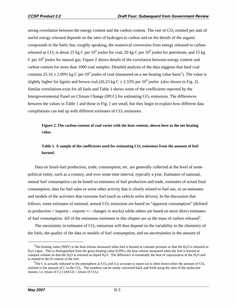
CCSP Product 2.2 Draft Four: Subsequent from Government Review
May 2007 II-3
strong correlation between the energy content and the carbon content. The rate of CO2 emitted per unit of
useful energy released depends on the ratio of hydrogen to carbon and on the details of the organic
compounds in the fuels; but, roughly speaking, the numerical conversion from energy released to carbon
released as CO2 is about 25 kg C per 109 joules for coal, 20 kg C per 109 joules for petroleum, and 15 kg
C per 109 joules for natural gas. Figure 2 shows details of the correlation between energy content and
carbon content for more than 1000 coal samples. Detailed analysis of the data suggests that hard coal
contains 25.16 ± 2.09% kg C per 109 joules of coal (measured on a net heating value basis1). The value is
slightly higher for lignite and brown coal (26.23 kg C ± 2.33% per 109 joules (also shown in Fig. 2).
Similar correlations exist for all fuels and Table 1 shows some of the coefficients reported by the
Intergovernmental Panel on Climate Change (IPCC) for estimating CO2 emissions. The differences
between the values in Table 1 and those in Fig. 1 are small, but they begin to explain how different data
compilations can end up with different estimates of CO2 emissions.
Figure 2. The carbon content of coal varies with the heat content, shown here as the net heating
value.
Table 1. A sample of the coefficients used for estimating CO2 emissions from the amount of fuel
burned.
Data on fossil-fuel production, trade, consumption, etc. are generally collected at the level of some
political entity, such as a country, and over some time interval, typically a year. Estimates of national,
annual fuel consumption can be based on estimates of fuel production and trade, estimates of actual final
consumption, data for fuel sales or some other activity that is clearly related to fuel use, or on estimates
and models of the activities that consume fuel (such as vehicle miles driven). In the discussion that
follows, some estimates of national, annual CO2 emissions are based on “apparent consumption” (defined
as production + imports – exports +/– changes in stocks) while others are based on more direct estimates
of fuel consumption. All of the emissions estimates in this chapter are as the mass of carbon released2.
The uncertainty in estimates of CO2 emissions will thus depend on the variability in the chemistry of
the fuels, the quality of the data or models of fuel consumption, and on uncertainties in the amount of
1Net heating value (NHV) is the heat release measured when fuel is burned at constant pressure so that the H2O is released as H2O vapor. This is distinguished from the gross heating value (GHV), the heat release measured when the fuel is burned at constant volume so that the H2O is released as liquid H2O. The difference is essentially the heat of vaporization of the H2O and is related to the H content of the fuel. 2The C is actually released to the atmosphere as CO2 and it is accurate to report (as is often done) either the amount of CO2 emitted or the amount of C in the CO2. The numbers can be easily converted back and forth using the ratio of the molecular masses, i.e. (mass of C) x (44/12) = (mass of CO2).
CCSP Product 2.2 Draft Four: Subsequent from Government Review
May 2007 II-4
carbon that is used for non-fuel purposes (such as asphalt and plastics) or is otherwise not burned. For
countries like the United States—with good data on fuel production, trade, and consumption—the
uncertainty in national emissions of CO2 is on the order of ± 5% or less. In fact, the US Environmental
Protection Agency (USEPA, 2005) suggests that their estimates of CO2 emissions from energy use in the
United States are accurate, at the 95% confidence level, within –1 to +6 % and Environment Canada
(2005) suggests that their estimates for Canada are within –4 to 0 %. The Mexican National Report
(Mexico, 2001) does not provide estimates of uncertainty, but our analyses with the Mexican data suggest
that uncertainty is larger than for the United States and Canada. Emissions estimates for these same three
countries, as reported by the Carbon Dioxide Information Analysis Center (CDIAC) and the International
Energy Agency (IEA) (see the following section), will have larger uncertainty because these groups are
making estimates for all countries. Because they work with data from all countries, they use global
average values for things like the emissions coefficients, whereas agencies within the individual countries
use values that are more specific to the particular country. When national emissions are calculated by
consistent methods it is likely that year-to-year changes can be estimated more accurately than would be
suggested by the uncertainties of the individual annual values.
1.2 The Magnitude of National and Regional CO2 Emissions
Figure 3 shows that from the beginning of the fossil-fuel era (1751 in these graphs) to the end of
2002, there were 93.5 Gt C released as CO2 from fossil-fuel consumption (and cement manufacture) in
North America: 84.4 Gt C from the United States, 6.0 from Canada, and 3.1 from Mexico. All three
countries of North America are major users of fossil fuels and this 93.5 Gt C was 31.5 % of the global
total. Among all countries, the United States, Canada, and Mexico ranked as the first, eighth, and eleventh
largest emitters of CO2 from fossil-fuel consumption, respectively (for 2002) (Marland et al., 2005).
Figure 4 shows, for each of these countries and for the sum of the three, the annual total of emissions and
the contributions from the different fossil fuels.
Figure 3. The cumulative total of CO2 emissions from fossil-fuel consumption and cement
manufacture, as a function of time, for the three countries of North America and for the sum of the
three.
Figure 4. Annual emissions of CO2 from fossil-fuel use by fuel type.
The long time series of emissions estimates in Figs. 1, 3, and 4 are from the CDIAC (Marland et al.,
2005). These estimates are derived from the “apparent consumption” of fuels and are based on data from

CCSP Product 2.2 Draft Four: Subsequent from Government Review
May 2007 II-5
the UN Statistics Office back to 1950 and on data from a mixture of sources for the earlier years (Andres
et al., 1999). There are other published estimates (with shorter time series) of national, annual CO2
emissions. Most notably the IEA (2005) has reported estimates of emissions for many countries for all
years back to 1971, and most countries have now provided some estimates of their own emissions as part
of their national obligations under the United Nations Framework Convention on Climate Change
(UNFCCC, see http://unfccc.int). These latter two sets of estimates are based on data on actual fuel
consumption and thus are able to provide details as to the sector of the economy where fuel use is taking
place3.
Comparing the data from multiple sources can give us some insight into the reliability of the
estimates generally. These different estimates of CO2 emissions are not, of course, truly independent
because they all rely ultimately on national data on fuel use; but they do represent different manipulations
of this primary data and in many countries there are multiple potential sources of energy data. Many
developing countries do not collect or do not report all of the data necessary to precisely estimate CO2
emissions and in these cases differences can be introduced by how the various agencies derive the basic
data on fuel production and use. Because of the way data are collected, there are statistical differences
between “consumption” and “apparent consumption” as defined above.
To make comparisons of different estimates of CO2 emissions we would like to be sure that we are
indeed comparing estimates of the same thing. For example emissions from cement manufacture are not
available from all of the sources, so they are not included in the comparisons in Table 2. All of the
estimates in Table 2, except those from the IEA, include emissions from flaring natural gas at oil
production facilities. It is not easy to identify the exact reason the estimates differ, but the differences are
generally small. The differences have mostly to do with the statistical difference between consumption
and apparent consumption, the way in which correction is made for non-fuel usage of fossil-fuel
resources, the conversion from mass or volume to energy units, and/or the way in which estimates of
carbon content are derived. Because the national estimates from CDIAC do not include emissions from
the non-fuel uses of petroleum products, we expect them to be slightly smaller than the other estimates
shown here, all of which do include these emissions4. The comparisons in Table 2 reveal one number for
which there is a notable relative difference among the multiple sources, emissions from Mexico in 1990.
Losey (2004) has suggested, based on other criteria, that there is a problem in the United Nations energy
3The International Energy Agency provides estimates based on both the reference approach (estimates of apparent consumption) and the sectoral approach (estimates of actual consumption) as described by the IPCC (IPCC, 1997). In the comparison here we use the numbers that they believe to be the most accurate, those based on the sectoral approach. 4The CDIAC estimate of global total emissions does include estimates of emissions from oxidation from non-fuel use of hydrocarbons.

CCSP Product 2.2 Draft Four: Subsequent from Government Review
May 2007 II-6
data set with the Mexican natural gas data for the 3 years 1990-1992, and these kinds of analyses result in
re-examination of some of the fundamental data.
Table 2. Different estimates (in Mt C) of CO2 emissions from fossil-fuel consumption for the United
States, Canada, and Mexico.
The IEA (2005, p. 1.4) has systematically compared their estimates with those reported to the
UNFCCC by the different countries and they find that the differences for most developed countries are
within 5%. The IEA attributes most of the differences to the following: use of the IPCC Tier 1 method
that does not take into account different technologies, use of energy data that may have come from
different “official” sources within a country, use of average values for net heating value of secondary oil
products, use of average emissions values, use of incomplete data on non-fuel uses, different treatment of
military emissions, and a different split between what is identified as emissions from energy and
emissions from industrial processes.
1.3 Emissions by Month and/or State
With increasing interest in the details of the global carbon cycle there is increasing interest in
knowing emissions at spatial and temporal scales finer than countries and years. For the United States,
energy data have been collected for many years at the level of states and months and thus estimates of
CO2 emissions can be made by state or by month. Figure 5 shows the variation in U.S. emissions by
month and preliminary analyses by Gurney et al. (2005) reveal that proper recognition of this variability
can be very important in some exercises to model the details of the global carbon cycle.
Figure 5. Emissions of CO2 from fossil-fuel consumption in the United States, by month.
Because of differences in the way energy data are collected and aggregated, it is not obvious that an
estimate of emissions from the United States will be identical to the sum of estimates for the 50 U.S.
states. Figure 6 shows that estimates of total annual CO2 emissions are slightly different if we use data
directly from the U.S. Department of Energy (DOE) and sum the estimates for the 50 states or if we sum
the estimates for the 12 months of a given year, or if we take U.S. energy data as aggregated by the UN
Statistics Office and calculate the annual total of CO2 emissions directly. Again, the state and monthly
emissions data are based on estimates of fuel consumption while the national emissions estimates
calculated using UN data result from estimates of “apparent consumption.” There is a difference between
annual values for consumption and annual values of “apparent consumption” (the IEA calls this

CCSP Product 2.2 Draft Four: Subsequent from Government Review
May 2007 II-7
difference simply “statistical difference”) that is related to the way statistics are collected and aggregated.
There are also differences in the way values for fuel chemistry and non-fuel usage are averaged at
different spatial and temporal scales, but the differences in CO2 estimates are seen to be within the error
bounds generally expected.
Figure 6. A comparison of three different estimates of national, annual emissions of CO2 from fossil-
fuel consumption in the United States.
Data from DOE permit us to estimate emissions by state or by month (Blasing et al., 2005a and
2005b), but they do not permit us to estimate CO2 emissions for each state by month directly from the
published energy data. Nor do we have sufficiently complete data to estimate emissions from Canada and
Mexico by month or province. Andres et al. (2005), Gregg (2005), and Losey (2004) have shown that we
can disaggregate national total emissions by month or by some national subdivision (such as states or
provinces) if we have data on some large fraction of fuel use. Because this approach relies on determining
the fractional distribution of an otherwise-determined total, it can be done with incomplete data on fuel
use. The estimates will, of course, improve as the fraction of the total fuel use is increased. Figure 7 is
based on sales data for most fossil fuel commodities and the CDIAC estimates of total national emissions,
and shows how the CO2 emissions from North America vary at a monthly time scale.
Figure 7. CO2 emissions from fossil-fuel consumption in North America, by month.
1.4 Emissions by Economic Sector
To understand how CO2 emissions from fossil-fuel use interact in the global and regional cycling of
carbon, it is necessary to know the masses of emissions and their spatial and temporal patterns. We have
tried to summarize this information here. To understand the trends and the driving forces behind the
growth in fossil-fuel emissions, and the opportunities for controlling emissions, it is necessary to look in
detail at how the fuels are used. This is the goal of the next four chapters of this report.
Before looking at the details of how energy is used and where CO2 emissions occur in the economies
of North America, however, there are two indices of CO2 emissions at the national level that provide
perspective on the scale and distribution of emissions. These two indices are emissions per capita and
emissions per unit of economic activity, the latter generally represented by CO2 per unit of gross domestic
product (GDP). Figure 8 shows the 1950–2002 record of CO2 emissions per capita for the three countries
of North America and, for perspective, includes the same data for the Earth as a whole. Similarly, Table 3
shows CO2 emissions per unit of GDP for the three countries of North America and for the world total.
CCSP Product 2.2 Draft Four: Subsequent from Government Review
May 2007 II-8
These are, of course, very complex indices and though they provide some insight they say nothing about
the details and the distributions within the means. The data on CO2 per capita for the 50 U.S. states (Fig.
9) show that values range over a full order of magnitude, differing in complex ways with the structure of
the economies and probably with factors like climate, population density, and access to resources (Blasing
et al., 2005b; Neumayer, 2004).
Figure 8. Per capita emissions of CO2 from fossil-fuel consumption (and cement manufacture) in the
United States, Canada, and Mexico and for the global total of emissions.
Table 3. Emissions of CO2 from fossil-fuel consumption (cement manufacture and gas flaring are not
included) per unit of GDP for the United States, Canada, and Mexico and for the global total.
Figure 9. Per capita emissions of CO2 from fossil-fuel consumption for the 50 United States in 2000.
Chapters 6 through 9 of this report discuss the patterns and trends of CO2 emissions by sector and the
driving forces behind the trends that are observed. Estimating emissions by sector brings special
challenges in defining sectors and assembling the requisite data. Readers will find that there is
consistency and coherence within each of the following chapters but will encounter difficulty in
aggregating or summing numbers across chapters. Different experts use different sector boundaries,
different data sources, different conversion factors, etc. Different analysts and literature sources will find
data for different base years and may treat electricity and biomass fuels differently. The national reports
of the United States, Canada, and Mexico do not cover the same time periods, nor do they present data in
the same way. In a discussion of the possibilities for reducing CO2 emissions in the building sector it is
not obvious, for example, whether to include the relevant electricity within the building sector, to leave
electric power generation as a separate sector, or to accept some overlap in the discussion. The authors of
Chapters 6, 7, 8, and 9 have chosen the system boundaries and data they find most useful for the
individual sectors, even though it makes it more difficult to aggregate across sectors.
Despite these differences in accounting procedures, the four chapters that follow accurately
characterize the patterns of emissions and the opportunities for controlling the growth in emissions. They
reveal that there are major differences between the countries of North America where, for example, the
United States derives 51% of its electricity from coal, Mexico gets 68% from petroleum and natural gas,
and Canada gets 58% from hydroelectric stations. Partially as a reflection of this difference, 40% of U.S.
CO2 emissions are from enterprises whose primary business is to generate electricity and heat, while this
number is only 31% in Mexico and 23% in Canada (for 2003; from IEA, 2005). Chapter 8 reveals that the
CCSP Product 2.2 Draft Four: Subsequent from Government Review
May 2007 II-9
sectors are not independent as, for example, a change from fuel burning to electricity in an industrial
process will decrease emissions from the industrial sector but increase emissions in the electric power
sector. The database of the IEA allows us to summarize CO2 emissions for the three countries according
to sectors that closely correspond to the sectoral division of chapters 6 through 9 (Table 4).
Table 4. Percent of CO2 emissions by sector for 2003.
2. CONCLUSION
There are a variety of reasons that we want to know the emissions of CO2 from fossil fuels, there are a
variety of ways of coming up with the desired estimates, and there are a variety of ways of using the
estimates. By the nature of the process of fossil-fuel combustion, and because of its economic importance,
there are reasonably good data over long time intervals that we can use to make reasonably accurate
estimates of CO2 emissions to the atmosphere. In fact, it is the economic importance of fossil-fuel burning
that has assured us of both good data on emissions and great challenges in altering the rate of emissions.
REFERENCES FOR PART II OVERVIEW
Andres, R.J., D.J. Fielding, G. Marland, T.A. Boden, N. Kumar, and A.T. Kearney, 1999: Carbon dioxide emissions
from fossil-fuel use, 1751–1950. Tellus, 51, 759–765.
Andres, R.J., J.S. Gregg, L.M. Losey, and G. Marland, 2005: Monthly Resolution Fossil-Fuel-Derived Carbon
Dioxide Emissions for the Countries of the North American Carbon Program. Proceedings of the Seventh
International Carbon Dioxide Conference, Bloomfield, CO, September, 2005, pp. 157–158.
Blasing, T.J., C.T. Broniak, and G. Marland, 2005a: The annual cycle of fossil-fuel carbon dioxide emissions in the
United States. Tellus, 57B, 107–115. (data available at http://cdiac.esd.ornl.gov)
Blasing, T.J., C. Broniak, and G. Marland, 2005b: State-by-state carbon dioxide emissions from fossil-fuel use in
the United States 1960–2000. Mitigation and Adaptation Strategies for Global Change, 10, 659–674.
Environment Canada, 2005: Canada’s Greenhouse Gas Inventory: 1990–2003. National Inventory Report, April
15, 2005, Greenhouse Gas Division, Environment Canada.
Gregg, J.S., 2005: Improving the Temporal and Spatial Resolution of Carbon Dioxide Emissions Estimates from
Fossil-Fuel Consumption. A thesis submitted to the graduate faculty of the University of North Dakota, August,
2005, 404 pp. (data available at http://cdiac.esd.ornl.gov)
Gurney, K.R., Y.H Chen, T. Maki, S.R. Kawa, A. Andrews, and Z. Zhu, 2005: Sensitivity of atmospheric CO2
inversion to seasonal and interannual variations in fossil-fuel emissions. Journal of Geophysical Research,
110(D10), 10308.
IEA, 2005: CO2 Emissions from Fuel Combustion: 1971–2003. International Energy Agency, OECD/IEA, Paris,
France.
CCSP Product 2.2 Draft Four: Subsequent from Government Review
May 2007 II-10
IPCC (Intergovernmental Panel on Climate Change), 1997: Revised 1996 IPCC Guidelines for National
Greenhouse Gas Inventories (3 Volumes). IPCC Technical Support Unit, Bracknell, United Kingdom.
Losey, L.M., 2004: Monthly and Seasonal Estimates of Carbon Dioxide Emissions from Fossil Fuel Consumption in
Canada, Mexico, Brazil, The United Kingdom, France, Spain, Italy, and Poland. A thesis submitted to the
graduate faculty of the University of North Dakota, May, 2004, 328 pp. (data available at
http://cdiac.essd.ornl.gov)
Marland, G., T. Boden, and R.J. Andres, 1995: Carbon dioxide emissions from fossil fuel burning: emissions
coefficients and the global contribution of eastern European countries. Időjárás, 99, 157–170.
Marland, G., T.A. Boden, and R.J. Andres, 2005: Global, regional, and national CO2 emissions. In: Trends: A
Compendium of Data on Global Change. Carbon Dioxide Information Analysis Center, Oak Ridge National
Laboratory, U.S. Department of Energy, Oak Ridge, TN, U.S.A. Available at http://cdiac.esd.ornl.gov
Mexico, 2001: México: Segunda comunicación nacional ante la Convención Marco de las Naciones Unidas sobre
el cambio climático. Comité intersecretarial sobre cambio climático, Secretaria de Medio Ambiente y Recursos
Naturales (Semarnat), Mexico City, 374 pp.
Neumayer, E., 2004: National carbon dioxide emissions: geography matters. Area, 36(1), 33–40.
USEPA, 2005: Inventory of U.S. Greenhouse Gas Emissions and Sinks: 1990–2003. EPA 430-R-05-003, United
States Environmental Protection Agency, Washington, DC.

CCSP Product 2.2 Draft Four: Subsequent from Government Review
May 2007 II-11
Table 1. A sample of the coefficients used for estimating CO2 emissions from the amount of fuel burned
Fuel Emissions coefficient (kg C/109 J net heating value)
Lignite 27.6 Anthracite 26.8 Bituminous coal 25.8 Crude oil 20.0 Residual fuel oil 21.1 Diesel oil 20.2 Jet kerosene 19.5 Gasoline 18.9 Natural gas 15.3 Source: IPCC, 1997.
Table 2. Different estimates (in Mt C) of CO2 emissions from fossil-fuel consumption for the United States, Canada, and Mexico
Country 1990 1998 2002 United States
CDIAC
1305
CDIAC
1501
CDIAC
1580
IEA 1320 IEA 1497 IEA 1545 USEPA 1316 USEPA 1478 USEPA 1534 Canada
CDIAC
112
CDIAC
119
CDIAC
139
IEA 117 IEA 136 IEA 145 Canada 117 Canada 133 Canada 144 Mexico
CDIAC
99
CDIAC
96
CDIAC
100
IEA 80 IEA 96 IEA 100 Mexico 81 Mexico 96 Mexico NA
Notes: Many of these data were published in terms of the mass of CO2, and these data have been multiplied by 12/44 to get the mass of carbon for the comparison here. All data except CDIAC include oxidation of non-fuel hydrocarbons. All data except IEA include flaring of gas at oil and gas processing facilities. Sources: CDIAC (Marland et al., 2005), IEA (2005), USEPA (2005), Canada (Environment Canada, 2005), and Mexico (2001).
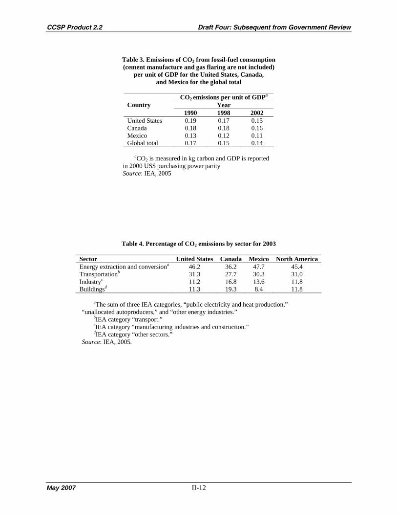
CCSP Product 2.2 Draft Four: Subsequent from Government Review
May 2007 II-12
Table 3. Emissions of CO2 from fossil-fuel consumption (cement manufacture and gas flaring are not included)
per unit of GDP for the United States, Canada, and Mexico for the global total
CO2 emissions per unit of GDPa
Year Country 1990 1998 2002
United States 0.19 0.17 0.15 Canada 0.18 0.18 0.16 Mexico 0.13 0.12 0.11 Global total 0.17 0.15 0.14
aCO2 is measured in kg carbon and GDP is reported in 2000 US$ purchasing power parity Source: IEA, 2005
Table 4. Percentage of CO2 emissions by sector for 2003
Sector United States Canada Mexico North America Energy extraction and conversiona 46.2 36.2 47.7 45.4 Transportationb 31.3 27.7 30.3 31.0 Industryc 11.2 16.8 13.6 11.8 Buildingsd 11.3 19.3 8.4 11.8
aThe sum of three IEA categories, “public electricity and heat production,” “unallocated autoproducers,” and “other energy industries.” bIEA category “transport.” cIEA category “manufacturing industries and construction.” dIEA category “other sectors.” Source: IEA, 2005.

CCSP Product 2.2 Draft Four: Subsequent from Government Review
May 2007 II-13
Fig. 1. Cumulative global emissions of CO2 from fossil-fuel combustion and cement manufacture from 1751 to 2002. Source data: Marland et al., 2005.

CCSP Product 2.2 Draft Four: Subsequent from Government Review
May 2007 II-14
Net Heating Value (dry, BTU/lb)5000 7000 9000 11000 13000 15000
Coal C
Content (dry, %
)
40
60
80
100
Carbon Content Versus Heating Value1063 Samples from the Penn State Coal Database
Lig
nite
C C
onte
nt (d
ry, %
)
20
40
60
80
125 lignites
938 coals
Fig. 2. The carbon content of coal varies with the heat content, shown here as
the net heating value. To make them easier to distinguish, data for lignites and brown coals are shown on the left axis, while data for hard coals are offset by 20% and shown on the right axis. Heating value is plotted in the units at which it was originally reported, Btu/lb, where 1 Btu/lb = 2324 J/kg. Source: Marland et al., 1995.
Fig. 3. The cumulative total of CO2 emissions from fossil-fuel consumption and
cement manufacture, as a function of time, for the three countries of North America and for the sum of the three. Source: Marland et al., 2005.

CCSP Product 2.2 Draft Four: Subsequent from Government Review
May 2007 II-15
Fig. 4A and 4B. Annual emissions of CO2 from fossil-fuel use by fuel type.
Figure 4A is for the United States, Figure 4B is for Canada, Figure 4C is for Mexico, and Figure 4D is for the sum of the three. Note that in order to illustrate the contributions of the different fuels, the four plots are not to the same vertical scale. Source: Marland et al., 2005.
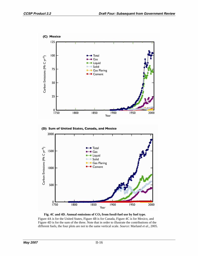
CCSP Product 2.2 Draft Four: Subsequent from Government Review
May 2007 II-16
Fig. 4C and 4D. Annual emissions of CO2 from fossil-fuel use by fuel type.
Figure 4A is for the United States, Figure 4B is for Canada, Figure 4C is for Mexico, and Figure 4D is for the sum of the three. Note that in order to illustrate the contributions of the different fuels, the four plots are not to the same vertical scale. Source: Marland et al., 2005.

CCSP Product 2.2 Draft Four: Subsequent from Government Review
May 2007 II-17
0
25
50
75
100
125
150
1982
1984
1986
1988
1990
1992
1994
1996
1998
2000
2002
2004
CO
2 Em
issi
ons
(Mt C
per
mon
th)
Total Coal Oil Gas
Fig. 5. Emissions of CO2 from fossil-fuel consumption in the United States, by month. Emissions from cement manufacturing are not included. Source: Blasing et al., 2005a.

CCSP Product 2.2 Draft Four: Subsequent from Government Review
May 2007 II-18
Fig. 6. A comparison of three different estimates of national annual emissions
of CO2 from fossil-fuel consumption in the United States. (6A) Estimates from U.S. Department of Energy data on fuel consumption by state (blue squares) vs. estimates based on UN Statistics Office data on apparent fuel consumption for the full United States (red squares). Source: Marland et al., 2003. (6B) Estimates based on DOE data on fuel consumption in the 50 U.S. states (blue squares) vs. estimates based on national fuel consumption for each of the 12 months (red squares). The state and monthly data include estimates of oxidation of non-fuel hydrocarbon products; the UN-based estimates do not. Source: Blasing et al., 2005b.

CCSP Product 2.2 Draft Four: Subsequent from Government Review
May 2007 II-19
Fig. 7. CO2 emissions from fossil-fuel consumption in North America, by month. Monthly values are shown where estimates are justified by the availability of monthly data on fuel consumption or sales. Source: Andres et al., 2005.
Fig. 8. Per capita emissions of CO2 from fossil-fuel consumption (and cement manufacture) in the United States, Canada, and Mexico and for the global total of emissions. Source: Marland et al., 2005.

CCSP Product 2.2 Draft Four: Subsequent from Government Review
May 2007 II-20
Fig. 9. Per capita emissions of CO2 from fossil-fuel consumption for the 50 United States in 2000. To demonstrate the range, values have been rounded to whole numbers of metric tons carbon per capita. A large portion of the range for extreme values is related to the occurrence of coal resources and inter-state transfers of electricity. Source: Blasing et al., 2005b.
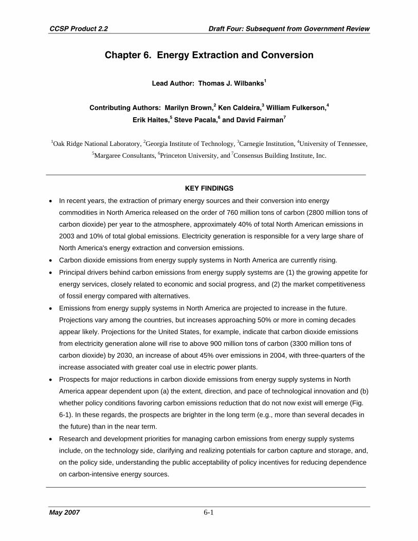
CCSP Product 2.2 Draft Four: Subsequent from Government Review
May 2007 6-1
Chapter 6. Energy Extraction and Conversion
Lead Author: Thomas J. Wilbanks1
Contributing Authors: Marilyn Brown,2 Ken Caldeira,3 William Fulkerson,4
Erik Haites,5 Steve Pacala,6 and David Fairman7
1Oak Ridge National Laboratory, 2Georgia Institute of Technology, 3Carnegie Institution, 4University of Tennessee,
5Margaree Consultants, 6Princeton University, and 7Consensus Building Institute, Inc.
KEY FINDINGS
• In recent years, the extraction of primary energy sources and their conversion into energy
commodities in North America released on the order of 760 million tons of carbon (2800 million tons of
carbon dioxide) per year to the atmosphere, approximately 40% of total North American emissions in
2003 and 10% of total global emissions. Electricity generation is responsible for a very large share of
North America's energy extraction and conversion emissions.
• Carbon dioxide emissions from energy supply systems in North America are currently rising.
• Principal drivers behind carbon emissions from energy supply systems are (1) the growing appetite for
energy services, closely related to economic and social progress, and (2) the market competitiveness
of fossil energy compared with alternatives.
• Emissions from energy supply systems in North America are projected to increase in the future.
Projections vary among the countries, but increases approaching 50% or more in coming decades
appear likely. Projections for the United States, for example, indicate that carbon dioxide emissions
from electricity generation alone will rise to above 900 million tons of carbon (3300 million tons of
carbon dioxide) by 2030, an increase of about 45% over emissions in 2004, with three-quarters of the
increase associated with greater coal use in electric power plants.
• Prospects for major reductions in carbon dioxide emissions from energy supply systems in North
America appear dependent upon (a) the extent, direction, and pace of technological innovation and (b)
whether policy conditions favoring carbon emissions reduction that do not now exist will emerge (Fig.
6-1). In these regards, the prospects are brighter in the long term (e.g., more than several decades in
the future) than in the near term.
• Research and development priorities for managing carbon emissions from energy supply systems
include, on the technology side, clarifying and realizing potentials for carbon capture and storage, and,
on the policy side, understanding the public acceptability of policy incentives for reducing dependence
on carbon-intensive energy sources.

CCSP Product 2.2 Draft Four: Subsequent from Government Review
May 2007 6-2
Figure 6-1. Prospects for carbon emissions from energy extraction and conversion in North
America, assuming substantial improvement in energy efficiency.
1. INTRODUCTION
The energy supply system in North America is a significant part of the North American carbon cycle,
because so many of its primary energy resources are fossil fuels, associated with extraction and
conversion activities that emit greenhouse gases. This chapter summarizes the knowledge bases related to
emissions from energy extraction, energy conversion, and other energy supply activities such as energy
movement and energy storage, along with options and measures for managing emissions.
Clearly, this topic overlaps the subject matter of other chapters. For instance, the dividing line
between energy conversion and other types of industry is sometimes indistinct. One prominent case is
emissions associated with electricity and process heat supply for petroleum refining and other fossil-fuel
processing – a large share of their total emissions, included in industrial sector emission totals; another
example is industrial co-generation as an energy-efficiency strategy. In addition, biomass energy
extraction/conversion is directly related to agriculture and forestry. Moreover, emission-related policy
alternatives for energy supply systems are often directed at both supply and demand responses, involving
not only emission reductions but also potential payoffs from efficiency improvements in buildings,
industry, and transportation, especially where they reduce the consumption of fossil fuels.
2. CARBON EMISSIONS INVENTORY
2.1 Carbon Emissions from Energy Extraction and Conversion
Carbon emissions from energy resource extraction, conversion into energy commodities, and
transmission are one of the “big three” sectors accounting for most of the total emissions from human
systems in North America, along with industry and transportation. The largest share of total emissions
from energy supply (not including energy end use) is from coal and other fossil fuel use in producing
electricity; fossil-fuel conversion activities such as oil refining and natural gas transmission and
distribution also contribute to this total, but in much smaller amounts. Other emission sources are less
well defined but generally small, such as emissions from oil production and methane from reservoirs
established partly to support hydropower production (Tremblay et al., 2004), or from materials production
(e.g., metals production) associated with other renewable or nuclear energy technologies. Generally, data
on emissions have a relatively low level of uncertainty, although the source materials do not include
quantitative estimates of uncertainty.
Data on emissions from energy supply systems are unevenly available for the countries of North
America, and none are associated with sufficient information to support an assessment of uncertainty.

CCSP Product 2.2 Draft Four: Subsequent from Government Review
May 2007 6-3
Most emission data sets are organized by fuel consumed rather than by consuming sector, and countries
differ in sectors identified and the units of measurement. As a result, inventories are reported in this
chapter by country in whatever forms are available rather than constructing a North American inventory
that could not be consistent across all three major countries. It is worth noting that Canada and Mexico
export energy supplies to the United States; therefore, some emissions from energy supply systems in
these countries are associated with energy uses in the United States.
2.1.1 Canada
Canada is the world’s fifth-largest energy producing country, a significant exporter of both natural
gas and electricity to the United States. In Alberta, which produces nearly two-thirds of Canada’s energy,
energy accounts for about one-quarter of the province’s economic activity; its oil sands are estimated to
have more potential energy value than the remaining oil reserves of Saudi Arabia (U.S. Department of
Energy, 2004). Although Canada has steadily reduced its energy and carbon intensities since the early
1970s, its overall energy intensity remains high—in part due to its prominence as an energy producer—
and total greenhouse gas emissions have grown by 9% since 1990. As of 2003, greenhouse gas emissions
were 36.5 million tons of carbon (Mt C) equivalents (134 million tons of carbon dioxide [Mt CO2]
equivalents) for electricity and heat generation and 19 Mt C (71 Mt CO2) for petroleum refining and
upgrading and other fossil-fuel production (Environment Canada, 2003). Although the mix of carbon
dioxide (CO2) and methane (CH4) in these figures is unclear, the carbon emission equivalent is probably
within the range of 60-80 Mt C.
2.1.2 Mexico
Mexico is one of the largest sources of energy-related greenhouse gas emissions in Latin America,
although its per capita emissions are well below the per capita average of industrialized countries. The
first large oil-producing nation to ratify the Kyoto Protocol, it has promoted shifts to natural gas use to
reduce greenhouse gas emissions. The most recent emission figures are from the country’s Second
National Communication to the UN United Nations Framework Convention on Climate Change in 2001,
which included relatively comprehensive data from 1996 and some data from 1998. In 1998, total
emissions from “energy industries” were 13 Mt C (47.3 Mt CO2); from electricity generation they totaled
27.6 Mt C (101.3 Mt CO2); and “fugitive” emissions from oil and gas production and distribution were
between 1.4 and 2.0 Mt C (1.9 and 2.6 Mt of CH4), depending on the estimated “emission factor”
(Government of Mexico, 2001).

CCSP Product 2.2 Draft Four: Subsequent from Government Review
May 2007 6-4
2.1.3 United States
The United States is the largest national emitter of greenhouse gases in the world, and CO2 emissions
associated with electricity generation in 2004 account for 627 Mt C (2299 Mt CO2), or 39% of a national
total of 1600 Mt C (5890 Mt CO2) (EIA, 2006a). Greenhouse gases are also emitted from oil refining,
natural gas transmission, and other fossil energy supply activities, but apart from energy consumption
figures included in industry sector calculations, these emissions are relatively small compared with
electric power plant emissions. For instance, emissions from petroleum consumed in refining processes in
the United States are about 40 Mt C per year (EIA, 2004), while fugitive emissions from gas transmission
and distribution pipelines in the United States are about 2.2 Mt C per year.1 On the other hand, a study of
greenhouse gas emissions from a six-county area in southwestern Kansas found that compressor stations
for natural gas pipeline systems are a significant source of emissions at that local scale (AAG, 2003).
2.2 Carbon Sinks Associated with Energy Extraction and Conversion
Generally, energy supply in North America is based heavily on mining hydrocarbons from carbon
sinks accumulated over millions of years; but current carbon sequestration occurs in plant growth,
including the cultivation of feedstocks for bioenergy production. Limited strictly to energy sector
applications, the total contribution of these sinks to the North American carbon cycle is relatively small,
while other aspects of bioenergy development are associated with carbon emissions; but the substitution
of biomass-derived fuels (approximately emisson-neutral, as stored carbon is released with fuel use) for
fossil fuels represents a potentially significant net savings in emissions.
3. TRENDS AND DRIVERS
Three principal drivers are behind carbon emissions from energy extraction and conversion.
(1) The growing global and national appetite for energy services such as comfort, convenience,
mobility, and labor productivity, so closely related to progress with economic and social development and
the quality of life (Wilbanks, 1992). Globally, the challenge is to increase total energy services (not
necessarily supplies) over the next half-century by a factor of at least three or four—more rapidly than
overall economic growth—while reducing environmental impacts from the associated supply systems
(NAS, 1999). Mexico shares this need, while increases in Canada and the United States are likely to be
more or less proportional to rates of economic growth.
(2) The market competitiveness of fossil energy sources compared with supply- and demand-side
alternatives. Production costs of electricity from coal, oil, or natural gas at relatively large scales are
1 This numerical value represents the authors’ estimate; there is 95% certainty that this estimate is within 100%.
CCSP Product 2.2 Draft Four: Subsequent from Government Review
May 2007 6-5
currently lower than other sources, except large-scale hydropower, and production costs of liquid and gas
fuels are currently far lower than other sources, though rising. This is mainly because the energy density
and portability of fossil fuels is as yet unmatched by other energy sources, and in some cases policy
conditions reinforce fossil-fuel use. These conditions appear likely to continue for some years. In many
cases, the most cost-competitive alternative to fossil-fuel production and use is not alternative supply
sources but efficiency improvement.
(3) Enhanced future markets for alternative energy supply sources. In the longer run, however,
emissions from energy supply systems may—and in fact are likely to—begin to decline as alternative
technology options are developed and/or improved. Other possible driving forces for attention to
alternatives to fossil fuels, at least in the mid to longer term, include the possibility of shrinking oil and/or
gas reserves and changes in attitudes toward energy policy interventions.
Given the power of the first two of these drivers, total carbon emissions from energy extraction and
conversion in North America are currently rising (e.g., Fig. 6-2). National trends and drivers are as
follows. As is always the case, projections of the future involve higher levels of uncertainty than
measurements of the present, but source materials do not include quantitative estimates of uncertainties
associated with projections of future emissions.
Figure 6-2. U.S. carbon dioxide emissions from electricity generation, 1990-2004.
3.1 Canada
Canada has ratified the Kyoto Protocol, and it is seeking to meet the Kyoto target of CO2 emission
reduction to 6% below 1990 levels. Of these reductions, 25% are to be through domestic actions and 75%
through market mechanisms such as purchases of carbon credits (Government of Canada, 2005).
Domestic actions will include a significant reduction in coal consumption. Available projections,
however, indicate a total national increase of emissions in CO2 equivalent of 36.1% by 2020 from 1990
levels (Environment Canada, 2005). Emissions from electricity generation could increase 2000-2020 by
as much as two-thirds, while emissions from fossil-fuel production would remain relatively stable
(although substantial expansion of oil sands production could be a factor).
3.2 Mexico
It has been estimated that total Mexican CO2 emissions will grow 69% by 2010, although mitigation
measures could reduce this rate of growth by nearly half (Pew Center, 2002). Generally, energy sector
emissions in Mexico vary in proportion to economic growth (e.g., declining somewhat with a recession in
2001). However, factors, such as a pressing need for additional electricity supplies (calling for more than
CCSP Product 2.2 Draft Four: Subsequent from Government Review
May 2007 6-6
doubling production capacity between 1999 and 2008), could increase net emissions, while a national
strategy to promote greater use of natural gas (along with other policies related in part to concerns about
emissions associated with urban air pollution) could reduce emissions compared with a reference case
(EIA, 2005).
3.3 United States
The Energy Information Administration (EIA, 2006b) projects that emissions from electricity
generation in the United States between 2004 and 2030 will rise from about 627 Mt C (2299 Mt CO2) to
more than 900 Mt C (3300 Mt CO2), an increase of about 45%, with three-quarters of the increase
associated with greater coal use in electric power plants. EIA projects that technology advances could
lower emissions by as much as 9%. Projections of other emissions from energy supply systems appear to
be unavailable, but emissions could be expected to rise at a rate just below the rate of change in product
consumption in the U.S. economy.
4. OPTIONS FOR REDUCING EMISSIONS FROM ENERGY EXTRACTION AND
CONVERSION
Few aspects of the carbon cycle have received more attention in the past several decades than
emissions from fossil energy extraction and conversion. As a result, there is a wide array of technology
and policy options, many of which have been examined in considerable detail, although there is not a
strong consensus on courses of action.
4.1 Technology Options
Technology options for reducing energy-supply-related emissions (other than reduced requirements
due to end-use efficiency improvements) consist of:
• reducing emissions from fossil energy extraction, production, and movement (e.g., for electricity
generation by improving the efficiency of existing power plants or moving toward the use of lower-
emission technologies such as coal gasification-combined cycle generation facilities) and
• shifting from fossil energy sources to other energy sources [e.g., energy from the sun (renewable
energy) or from the atom (nuclear energy)].
The most comprehensive description of emission-reducing and fuel switching technologies and their
potentials is the U.S. Climate Change Technology Program (CCTP) draft Strategic Plan (U.S. Climate

CCSP Product 2.2 Draft Four: Subsequent from Government Review
May 2007 6-7
Change Technology Program, 2005), especially Chapters 5 (energy supply) and 6 (capturing and
sequestering CO2)—see also National Laboratory Directors (1997). The CCTP report focuses on five
energy supply technology areas: low-emission fossil-based fuels and power, hydrogen as an energy
carrier, renewable energy and fuels, nuclear fission, and fusion energy.
There is a widespread consensus that no one of these options, nor one family of options, is a good
prospect to stabilize greenhouse gas emissions from energy supply systems, nationally or globally,
because each faces daunting constraints (Hoffert et al., 2002). An example is possible physical and/or
technological limits to effective global “decarbonization” (i.e., reducing the use of carbon-based energy
sources as a proportion of total energy supplies), including renewable or other non-fossil sources of
energy use at scales that would dramatically change the global carbon balance between now and 2050.
One conclusion is that “the disparity between what is needed and what can be done without great
compromise may become more acute.”
Instead, progress with technologies likely to be available in the coming decades may depend on
adding together smaller “wedges” of contributions by a variety of resource/technology combinations
(Pacala and Socolow, 2004), each of which may be feasible if the demands upon it are moderate. If many
such contributions can be combined, the total effect could approach requirements for even relatively
ambitious carbon stabilization goals, at least in the first half of the century, although each contribution
would need to be economically competitive with current types of fossil energy sources.
A fundamental question is whether prospects for significant decarbonization depend on the
emergence of new technologies, in many cases requiring advances in science. For instance, efforts are
being made to develop economically affordable and socially acceptable options for large-scale capture of
carbon from fossil-fuel streams—with the remaining hydrogen offering a clean energy source—and
sequestration of the carbon in the ground or the oceans. This approach is known to be technologically
feasible (and is being practiced commercially in the North Sea), and recent assessments suggest that it
may have considerable promise (e.g., IPCC, 2006). If so, there is at least some chance that fossil energy
sources may be used to provide energy services in North America and the world in large quantities in the
mid to longer terms without contributing to a carbon cycle imbalance.
What can be expected from technology options over the next quarter to half a century is a matter of
debate, partly because the pace of technology development and use depends heavily on policy conditions.
Chapter 3 in the CCTP draft Strategic Plan (2005) shows three advanced technology scenarios drawn
from work by the Pacific Northwest National Laboratory, varying according to carbon constraints.
Potential cumulative contributions to global emission reduction by energy supply technology initiatives
between 2000 and 2100 range from about 25 billion tons of carbon (Gt C) equivalent to nearly 350 Gt,
which illustrates uncertainties related to both science and policy issues. Carbon capture and storage, along

CCSP Product 2.2 Draft Four: Subsequent from Government Review
May 2007 6-8
with terrestrial sequestration, could add reductions between about 100 and 325 Gt C. It has been
suggested, however, that significantly decarbonizing energy systems by 2050 could require massive
efforts on a par with the Manhattan project or the Apollo space program (Hoffert et al., 2002).
Estimated costs of potential technology alternatives for reducing greenhouse gas emissions from
energy supply systems are summarized after the following discussion of policy options, because cost
estimates are generally based on assumptions about policy interventions.
4.2 Policy Options
Policy options for carbon emission reduction from energy supply systems revolve around either
incentives or regulatory requirements for such reductions. Generally, interventions may be aimed at (a)
shaping technology choice and use or (b) shaping technology development and supply. Many of the
policy options are aimed at encouraging end-use efficiency improvement as well as supply-side emission
reduction.
Options for intervening to change the relative attractiveness of available energy supply technology
alternatives include appealing to voluntary action (e.g., improved consumer information, “green power”),
a variety of regulatory actions (e.g., mandated purchase policies such as energy portfolio standards),
carbon emission rights trading (where emission reduction would have market value), technology/product
standards, production tax credits for non-fossil energy production, tax credits for alternative energy use,
and carbon emission taxation or ceilings. Options for changing the relative attractiveness of investing in
carbon-emission-reducing technology development and dissemination include tax credits for certain kinds
of energy R&D, public-private sector R&D cost sharing, and electric utility restructuring. For a more
comprehensive listing and discussion, see Chapter 6 in IPCC (2001, Chapter 6).
In some cases, perceptions that policies and market conditions of the future will be more favorable to
emission reduction than at present are motivating private industry to consider investments in technologies
whose market competitiveness would grow in such a future. Examples include the CO2 Capture Project
and industry-supported projects at MIT, Princeton, and Stanford (e.g., see
http://www.co2captureproject.org/index.htm).
Most estimates of the impacts of energy policy options on greenhouse gas emissions do not
differentiate the contributions from energy supply systems from the rest of the energy economy [e.g.,
Interlaboratory Working Group (IWG), 1997; IWG, 2000; IPCC, 2001; National Commission on Energy
Policy, 2004; also see OTA, 1991, and NAS, 1992]. For instance the IWG (1997) considered effects of
$25 and $50 per ton carbon emission permits on both energy supply and use, while IWG considered fifty
policy/technology options (IWG, 2000; also see IPCC, 2001), most of which would affect both energy
supply and energy use decisions.

CCSP Product 2.2 Draft Four: Subsequent from Government Review
May 2007 6-9
4.3 Estimated Costs of Implementation
Estimating the costs of emission reduction associated with the implementation of various technology
and policy options for energy supply and conversion systems is complicated by several realities. First,
many estimates are aggregated for the United States or the world as a whole, without separate estimates
for the energy extraction and conversion sector. Second, estimates differ in the scenarios considered, the
modeling approaches adopted, and the units of measure that are used.
More specifically, estimates of costs of emission reduction vary widely according to assumptions
about such issues as how welfare is measured, ancillary benefits, and effects in stimulating technological
innovation; and therefore any particular set of cost estimate includes considerable uncertainty. According
to IWG (2000), benefits of emission reduction would be comparable to costs, and the National
Commission on Energy Policy (2004) estimates that their recommended policy initiatives would be,
overall, revenue-neutral with respect to the federal budget. Other participants in energy policymaking,
however, are convinced that truly significant carbon emission reductions would have substantial
economic impacts (GAO, 2004).
Globally, IPCC (2001) projected that total CO2 emissions from energy supply and conversion could
be reduced in 2020 by 350 to 700 Mt C equivalents per year, based on options that could be adopted using
generally accepted policies, at a positive direct cost of less than U.S. $100 per t C equivalents. Based on
DOE/EIA analyses in 2000, this study includes estimates of the cost of a range of specific emission-
reducing technologies for power generation, compared with coal-fired power, although the degree of
uncertainty is not clear. Within the United States, the report estimated that the cost of emission reduction
per metric ton of carbon emissions reduced would range from -$170 to +$880, depending on the
technology used. Marginal abatement costs for the total United States economy, in 1990 U.S. dollars per
metric ton carbon, were estimated by a variety of models compared by the Energy Modeling Forum at
$76 to $410 with no emission trading, $14 to $224 with Annex I trading, and $5 to $123 with global
trading.
Similarly, the National Commission on Energy Policy (2004) considered costs associated with a
tradable emission permit system that would reduce United States national greenhouse gas emission
growth from 44% to 33% from 2002 to 2025, a reduction of 207 Mt C (760 Mt CO2) in 2025 compared
with a reference case. The cost would be a roughly 5% increase in total end-use expenditures compared
with the reference case. Electricity prices would rise by 5.4% for residential users, 6.2% for commercial
users, and 7.6% for industrial users.
The IWG (2000) estimated that a domestic carbon trading system with a $25/t C permit price would
reduce emissions by 13%, or 63 Mt C (230 Mt CO2), compared with a reference case, while a $50 price

CCSP Product 2.2 Draft Four: Subsequent from Government Review
May 2007 6-10
would reduce emissions by 17 to 19%, or 83 to 91 Mt C (306 to 332 Mt CO2). Both cases assume a
doubling of United States government appropriations for cost-shared clean energy research, design, and
development.
For carbon capture and sequestration, IPCC (2006) concluded that this option could contribute 15 to
55% to global mitigation between now and 2100 if technologies develop as projected in relatively
optimistic scenarios and very large-scale geological carbon sequestration is publicly acceptable. Under
these assumptions, the cost is projected to be $110 to $260/t C ($30 to $70/t CO2). With less optimistic
assumptions, the cost could rise above $730/t C ($200/t CO2).
Net costs to the consumer, however, are balanced in some analyses by benefits from advanced
technologies, which are developed and deployed on an accelerated schedule due to policy interventions
and changing public preferences. The U.S. Climate Change Technology Program (2005: pp. 3-19)
illustrates how costs of achieving different stabilization levels can conceivably be reduced substantially
by the use of advanced technologies, and IWG (2000) estimates that net end-user costs of energy can
actually be reduced by a domestic carbon trading system if it accelerates the market penetration of more
energy-efficient technologies.
In many cases, however, discussions of the promise of technology options are not associated with cost
estimates. Economic costs of energy are not one of the drivers of the IPCC SRES scenarios, and such
references as Hoffert et al. (2002) and Pacala and Socolow (2004) are concerned with technological
potentials and constraints as a limiting condition on market behavior rather than with comparative costs
and benefits of particular technology options at the margin.
4.4 Summary
In terms of prospects for major emission reductions from energy extraction and conversion in North
America, the key issues appear to be the extent, direction, and pace of technological innovation and the
likelihood that policy conditions favoring carbon emissions reduction that do not now exist will emerge if
concerns about carbon cycle imbalances grow. In these regards, the prospects are brighter in the long term
(e.g., more than several decades in the future) than in the near term. History suggests that technology
solutions are usually easier to implement than policy solutions, but observed impacts of carbon cycle
imbalances might change the political calculus for policy interventions in the future.

CCSP Product 2.2 Draft Four: Subsequent from Government Review
May 2007 6-11
5. RESEARCH AND DEVELOPMENT NEEDS
If it is possible that truly effective management of carbon emissions from energy supply and
conversion systems cannot be realized with the current portfolio of technology alternatives under current
policy conditions, then research and development needs and opportunities deserve expanded attention and
support (e.g., National Commission on Energy Policy, 2004). If so, the priorities include
Technology. Several objectives seem to be especially relevant to carbon management potentials:
• clarifying and realizing potentials for carbon capture and sequestration;
• clarifying and realizing potentials of affordable renewable energy systems at a relatively large scale;
• addressing social concerns about the nuclear energy fuel cycle, especially in an era of concern about
terrorism;
• improving estimates of economic costs and emission reduction benefits of a range of energy;
technologies across a range of economic, technological, and policy scenarios; and
• “Blue Sky” research to develop new technology options and families, such as innovative approaches
for energy from the sun and from biomass, including possible applications of nanoscience (Caldeira et
al., 2005; Lewis, 2005).
Policy. Research and development could also be applied to policy options in order to enlarge their
knowledge bases and explore their implications. For instance, research priorities might include learning
more about:
• public acceptability of policy incentives for reducing dependence on energy sources associated with
carbon emissions,
• possible effects of incentives for the energy industry to increase its support for pathways not limited
to fossil fuels,
• approaches toward a more distributed electric power supply enterprise in which certain renewable
(and hydrogen) energy options might be more attractive,
• transitions from one energy system/infrastructure to another, and
• interactions and linkage effects among driving forces and responses, along with possible effects of
exogenous processes and policy interventions.
In these ways, technology and policy advances might be combined with multiple technologies to
transform the capacity to manage carbon emissions from energy supply systems, if that is a high priority
for North America.

CCSP Product 2.2 Draft Four: Subsequent from Government Review
May 2007 6-12
CHAPTER 6 REFERENCES
AAG, 2003: Global Change and Local Places: Estimating, Understanding, and Reducing Greenhouse Gases.
Association of American Geographers, Cambridge University Press, Cambridge, UK.
Caldeira, K., et al., 2005: Climate Change Technology Exploratory Research. Working paper, Climate Policy
Center, Washington, DC.
EIA, 2004: Emissions of Greenhouse Gases in the United States, 2004: Energy Information Administration,
Washington, DC.
EIA, 2005: International Energy Outlook, 2005: Energy Information Administration, Washington, DC.
EIA, 2006a: International Energy Outlook, 2006: Energy Information Administration, Washington, DC.
EIA, 2006b: Annual Energy Review, 2006: Energy Information Administration, Washington, DC.
Environment Canada, 2003: Canada’s Greenhouse Gas Inventory, 1990-2003. Available at
http://www.ec.gc.ca/pdb/ghg/inventory_report/2003_report/ts_2_e.cfm
Environment Canada, 2005: The Green Lane: Climate Change: The Greenhouse Gas Emissions Outlook to 2020.
Available at http://www.ec.gc.ca/climate/overview_2020-e.html
GAO (Government Accountability Office), 2004: Climate Change: Analysis of Two Studies of Estimated Costs of
Implementing the Kyoto Protocol. Washington, DC, January 2004.
Government of Canada, 2005: Project Green: Moving Forward on Climate Change. April 2005.
Government of Mexico, 2001: Second National Communication. Submitted to UNFCCC by the Secretaria de
Medio Ambiente y Recursos, Naturales, Mexico City.
Hoffert, M.I., et al., 2002: Advanced technology paths to global climate stability: energy for a greenhouse planet.
Science, 298, 981-987.
Interlaboratory Working Group, 1997: Scenarios of U.S. Carbon Reductions. Prepared by Lawrence Berkeley
National Laboratory (LBNL-40533) and Oak Ridge National Laboratory (ORNL/CON-444) for the U.S.
Department of Energy.
Interlaboratory Working Group, 2000: Scenarios for a Clean Energy Future. Prepared by Lawrence Berkeley
National Laboratory (LBNL-44029) and Oak Ridge National Laboratory (ORNL/CON-476) for the U.S.
Department of Energy.
IPCC, 2001: Climate Change, 2001: Mitigation. Contribution of Working Group III to the Third Assessment Report
of the Intergovernmental Panel on Climate Change. Cambridge University Press, Cambridge, UK.
IPCC, 2006: Carbon Dioxide Capture and Storage. IPCC Special Report. Cambridge University Press, Cambridge,
UK.
Lewis, N., 2005: Global Energy Perspective. Paper presented to the U.S. DOE Laboratory Energy and Development
Working Group (LERDWG), Washington, DC.
NAS (National Academy of Sciences), 1992: Policy Implications of Greenhouse Warming: Mitigation, Adaptation,
and the Science Base. Washington, DC.

CCSP Product 2.2 Draft Four: Subsequent from Government Review
May 2007 6-13
NAS (National Academy of Sciences), 1999: Our Common Journey: A Transition Toward Sustainability. National
Academy Press, Washington, DC.
National Commission on Energy Policy, 2004: Ending the Energy Stalemate: A Bipartisan Strategy to Meet
America’s Energy Challenges. NCEP, Washington, DC.
National Laboratory Directors, 1997: Technology Opportunities to Reduce U.S. Greenhouse Gas Emissions.
Prepared for the U.S. Department of Energy.
OTA (Office of Technology Assessment), 1991: Changing By Degrees: Steps to Reduce Greenhouse Gases.
OTA-0-482, Washington, DC.
Pacala, S. and R. Socolow, 2004: Stabilization wedges: solving the climate problem for the next 50 years with
current technologies. Science, 305, 968-972.
Pew Center on Global Climate Change, 2002: Climate Change Mitigation in Developing Countries. Report
prepared by W. Chandler, et al., Washington, DC.
Tremblay, A., 2004: Greenhouse Gas Emissions - Fluxes and Processes: Hydroelectric Reservoirs and Natural
Environments. Springer, New York, NY.
U.S. Climate Change Technology Program, 2005: Strategic Plan: Draft for Public Comment. Available at
http://www.climatetechnology.gov/stratplan/draft/index.htm
U.S. Department of Energy, 2004: National energy policy/overview/Canada. In: Energy Trends. Available at
http://energytrends.pnl.gov/Canada/ca004.htm
Wilbanks, T., 1992: Energy policy responses to concerns about global climate change. In: Global Climate Change:
Implications, Challenges and Mitigation Measures [Majumdar, S. et al., (eds.)]. Pennsylvania Academy of
Sciences, Easton, PA, pp. 452-470.

CCSP Product 2.2 Draft Four: Subsequent from Government Review
May 2007 6-14
Fig. 6-1. Prospects for carbon emissions from energy extraction and conversion in North America, assuming substantial improvements in energy efficiency.

CCSP Product 2.2 Draft Four: Subsequent from Government Review
May 2007 6-15
Fig. 6-2. U.S. carbon dioxide emissions from electricity generation, 1990-2004. Source: EIA, 2004, and the authors’ extensions for year 2004.
CCSP Product 2.2 Draft Four: Subsequent from Government Review
May 2007 6-16
[This page intentionally left blank]

CCSP Product 2.2 Draft Four: Subsequent from Government Review
May 2007 7-1
Chapter 7. Transportation
Lead Author: David L. Greene1
1Oak Ridge National Laboratory
KEY FINDINGS
• The transportation sector of North America released 587 million tons of carbon into the atmosphere in
2003, nearly all in the form of carbon dioxide from combustion of fossil fuels. This comprises 37% of
the total carbon dioxide emissions from worldwide transportation activity, which in turn, accounts for
about 22% of total global carbon dioxide emissions.
• Transportation energy use in North America and the associated carbon emissions have grown
substantially and relatively steadily over the past 40 years. Growth has been most rapid in Mexico,
the country most dependent upon road transport.
• Carbon emissions by transport are determined by the levels of passenger and freight activity, the
shares of transport modes, the energy intensity of passenger and freight movements, and the carbon
intensity of transportation fuels. The growth of passenger and freight activity is driven by population,
per capita income, and economic output.
• Chiefly as a result of economic growth, energy use by North American transportation is expected to
increase by 46% from 2003 to 2025. If the mix of fuels were assumed to remain the same, carbon
dioxide emissions would increase from 587 million tons of carbon in 2003 to 859 million tons of
carbon in 2025. Canada, the only one of the three countries in North America to have committed to
specific greenhouse gas reduction goals, is expected to show the lowest rate of growth in carbon
emissions.
• The most widely proposed options for reducing the carbon emissions of the North American
transportation sector are increased vehicle fuel economy, increased prices for carbon-based fuels,
liquid fuels derived from vegetation (biomass), and in the longer term, hydrogen produced from
renewable energy sources (such as hydropower), nuclear energy, or from fossil fuels with carbon
capture and storage. Biomass fuels appear to be a promising near- and long-term option, while
hydrogen could become an important energy carrier after 2025.
• After the development of advanced energy efficient vehicle technologies and low-carbon fuels, the
most pressing research need in the transportation sector is for comprehensive, consistent, and
rigorous assessments of carbon emissions mitigation potentials and costs for North America.

CCSP Product 2.2 Draft Four: Subsequent from Government Review
May 2007 7-2
1. BACKGROUND Transportation is the largest source of carbon emissions among North American energy end uses
(electricity generation is considered energy conversion rather than end use). This fact reflects the vast
scale of passenger and freight movements in a region that comprises one-fourth of the global economy, as
well as the dominance of relatively energy-intensive road transport and the near total dependence of
North American transportation systems on petroleum as a source of energy. If present trends continue,
carbon emissions from North American transportation are expected to increase by more than one-half by
2050. Options for mitigating carbon emissions from the transportation sector like increased vehicle fuel
economy and biofuels could offset the expected growth in transportation activity. However, at present
only Canada has committed to achieving a specific reduction in future greenhouse gas emissions: 6%
below 1990 levels by 2012 (Government of Canada, 2005).
2. INVENTORY OF CARBON EMISSIONS Worldwide, transportation produced about 22% (1.5 billion tons of carbon [Gt C]) of total global
carbon dioxide emissions from the combustion of fossil fuels (6.6 Gt C) in 2000 (page 3-1 in U.S. EPA,
2005; Marland, Boden and Andres, 2005). Home to 6.7% of the world’s 6.45 billion people and source of
24.8% of the world’s $55.5 trillion gross world product (CIA, 2005), North America produces 37% of the
total carbon emissions from worldwide transportation activity (Fulton and Eads, 2004).
Transportation activity is driven chiefly by population, economic wealth, and geography. Of the
approximately 435 million residents of North America, 68.0% reside in the United States, 24.5% in
Mexico, and 7.5% in Canada (CIA, 2005) (these population estimates are judged by the author to have
95% certainty that the actual value is within 10% of the estimate reported, and the GDP estimates are
judged to have 95% certainty that the actual value is within 25% of the estimate reported, chiefly because
they are not based on triple bottom accounting). The differences in the sizes of the three countries’
economies are far greater. The United States is the world’s largest economy, with an estimated gross
domestic product (GDP) of $11.75 trillion in 2004. Although Mexico has approximately three times the
population of Canada, its GDP is roughly the same, $1.006 trillion compared to $1.023 trillion (measured
in 2004 purchasing power parity dollars). With the largest population and largest economy, the United
States has by far the largest transportation system. The United States accounted for 87% of the energy
used for transportation in North America in 2003, Canada for 8%, and Mexico 5% (Fig. 7-1) (see Table 4-
1 in NATS, 2005). These differences in energy use are directly reflected in carbon emissions from the
CCSP Product 2.2 Draft Four: Subsequent from Government Review
May 2007 7-3
three countries’ transportation sectors (Table 7-1).1
Figure 7-1. Transportation energy use in North America, 1990-2003.
Table 7-1. Carbon emissions from transportation in North America in 2003.
Transportation is defined as private and public vehicles that move people and commodities (U.S.
EPA, 2005, p. 296). This includes automobiles, trucks, buses, motorcycles, railroads and railways
(including streetcars and subways), aircraft, ships, barges, and natural gas pipelines. This definition
excludes petroleum, coal slurry, and water pipelines, as well as the transmission of electricity, although
many countries consider all pipelines part of the transport sector. It also generally excludes mobile
sources not engaged in transporting people or goods, such as construction equipment, and on-farm
agricultural equipment. In addition, carbon emissions from international bunker fuel use in aviation and
waterborne transport, though considered part of transport emissions, are generally accounted for
separately from a nation’s domestic greenhouse gas inventory. In this chapter, however, they are included
as are carbon emissions from military transport operations because they are real inputs to the carbon
cycle. Upstream, or well-to-tank, carbon emissions are not included with transportation end-use, nor are
end-of-life emissions produced in the disposal or recycling of materials used in transportation vehicles or
infrastructure because these carbon flows are in the domain of other chapters. These two categories of
emissions typically comprise 20-30% of total life cycle emissions for transport vehicles (see Table 5.4 in
Weiss et al., 2000). In the future, it is likely that upstream carbon emissions will be of greater importance
in determining the total emissions due to transportation activities.
In addition to carbon dioxide, the combustion of fossil fuels by transportation produces other
greenhouse gases including methane (CH4), nitrous oxide (N2O), carbon monoxide (CO), nitrogen oxides
(NOx), and non-methane volatile organic compounds (VOCs). Those containing carbon are generally
oxidized in the atmosphere to ultimately produce CO2. However, the quantities of non-CO2 gases
produced by transportation vehicles are very minor sources of carbon in comparison to the volume of CO2
emissions. For example, North American emissions of CH4 by transportation accounted for only 0.03% of
total transportation carbon emissions in 2003. This chapter will therefore address primarily the carbon
dioxide emissions from transportation activities (methane emissions are included in the totals presented in
Table 7-1, but they are not included in any other estimates presented in this chapter). Estimates of non-
CO2 emissions are also subject to much greater uncertainty. INE (2003) generally put the accuracy of the
Mexican 2001 non-CO2 greenhouse gas emissions at 95% certainty that the actual value is within 50% of
1 Uncertainties in these estimates are discussed later in this chapter (see Section 5).

CCSP Product 2.2 Draft Four: Subsequent from Government Review
May 2007 7-4
the estimate reported. However, Environment Canada’s 2003 inventory (Environment Canada 2005) rates
the uncertainty of methane emissions from mobile sources as 95% certain that the actual value is within
10% of the estimate reported.
Four main sources of information on carbon emissions are used in this chapter. The estimates shown
in Table 7-1 were obtained from the greenhouse gas inventory reports of the three countries, estimated by
environmental agencies in accordance with IPCC guidelines. As Annex 1 countries, Canada and the
United States are obliged to compile annual inventories under IPCC guidelines. As a non-Annex 1
country, Mexico is not. These inventories are the most authoritative sources for estimates of carbon
emissions. The inventory reports, however, do not generally provide estimates of associated energy use
and the most recent inventory data available for Mexico are for 2001. Estimates of energy use and carbon
emissions produced by the countries’ energy agencies are also used in this chapter to illustrate the
relationship between energy use and carbon emissions and its historical trends. There are some minor
differences between the carbon emissions estimates from the two sources. Finally, future projections of
carbon emissions for North America to 2025 were taken from the U.S. Energy Information’s Annual
Energy Outlook 2005, and projections to 2050 were taken from the World Business Council on
Sustainable Development’s Sustainable Mobility Project (WBCSD, 2004).
2.1 Fuels Used in Transportation Virtually all of the energy used by the transport sector in North America is derived from petroleum,
and most of the remainder comes from natural gas (Table 7-2). In the United States, 96.3% of total
transportation energy is obtained by combustion of petroleum fuels (U.S. DOE/EIA, 2005a). Most of the
non-petroleum energy is natural gas used to power natural gas pipelines (2.5%, 744 petajoules). During the
past two decades, ethanol use as a blending component for gasoline has increased from a negligible
amount to 1.1% of transportation energy use (312 petajoules). Electricity, mostly for passenger rail
transport, comprises only 0.1% of United States transport energy use. This pattern of energy use has
persisted for more than half a century.
Table 7-2. Summary of North American transport energy use and carbon dioxide emissions in 2003
by fuel type.
The pattern of energy sources is only a little different in Mexico where 96.2% of transportation
energy use is gasoline, diesel, or jet fuel: 3.4% is liquefied petroleum gas, and less than 0.2% is electricity
(Rodríguez, 2005). In Canada, natural gas use for natural gas pipelines accounts for 7.5% of transport

CCSP Product 2.2 Draft Four: Subsequent from Government Review
May 2007 7-5
energy use, 91.8% is petroleum, 0.5% is propane and only 0.1% is electricity (see Table 1 in NRCan,
2006).
2.2 Mode of Transportation Mode of transportation refers to how people and freight are moved about, whether by road, rail, or air,
in light or heavy vehicles. Carbon dioxide emissions from the North American transportation sector are
summarized by mode in Table 7-3, and the distribution of emissions by mode for North America in 2003
is illustrated in Fig. 7-2.
Table 7-3. Summary of North American transport energy use and carbon dioxide emissions in 2003
by fuel type.
Figure 7-2. North American carbon emissions from transportation by mode; United States and
Canada 2003, Mexico 2001
2.2.1 Freight Transport Movement of freight is a major component of the transportation sector in North America. Total
freight activity in the United States, measured in metric ton-km, is 20 times that in Mexico and more than
10 times the levels observed in Canada (Figs. 7-3A, 7-3B, and 7-3C).
Figure 7-3A. Freight activity by mode in Canada.
Figure 7-3B. Freight activity by mode in Mexico.
Figure 7-3C. Freight activity by mode in the United States.
In Mexico, trucking is the mode of choice for freight movements. Four-fifths of Mexican metric ton-
km is produced by trucks. Moreover, trucking’s modal share has been increasing over time.
In Canada, rail transport accounts for the majority of freight movement (65%). Rail transport is well
suited to the approximately linear distribution of Canada’s population in close proximity to the United
States border, the long-distances from east to west, and the large volumes of raw material flows typical of
Canadian freight traffic (see Table 5-2 in NATS, 2005).
In the United States, road freight plays a greater role than in Canada, and rail is less dominant,
although rail still carries the largest share of metric ton-km (40%). In none of the countries does air
freight account for a significant share of metric ton-km.

CCSP Product 2.2 Draft Four: Subsequent from Government Review
May 2007 7-6
2.2.2 Passenger Transport In all three countries, passenger transport is predominantly by road, followed in distant second by air
travel. The rate of growth in air travel in North America is more than double that of road transport, so that
air transport’s share of carbon emissions will increase in the future. Nearly complete data are available for
passenger-kilometers-traveled (pkt) by mode in the United States and Canada in 2001. Of the more than 8
trillion pkt accounted for by the United States, 86% was by light-duty personal vehicles, most by
passenger car but a growing share by light trucks (Fig. 7-4A) (motorcycle pkt, about 0.2% of the total, is
included with passenger car). Air travel claims 10%; other modes are minor.
Figure 7-4A. Distribution of passenger travel in the United States by mode.
Canadian passenger travel exhibits a very similar modal structure, but with a smaller role played by
light trucks and air and a larger share for buses (Fig. 7-4B) (transit numbers for Canada were not available
at the time these figures were compiled).
Figure 7-4B. Distribution of passenger travel by mode in Canada.
3. TRENDS AND DRIVERS Driven by economic and population growth, transportation energy use has increased substantially in
all three countries since 1990. Figures 7-5A and 7-5B illustrate the evolution of transport energy use by
mode for Mexico and the United States. Energy use has grown most rapidly in Mexico, the country most
dependent on road transport. In the United States, the steady growth of transportation oil use was
interrupted by oil price shocks in 1973-74, 1979-80, and to a much lesser degree in 1991. The impact of
the attack on the World Trade Center in 2001 and subsequent changes in air travel procedures had a
visible effect on energy use for air travel.
Figure 7-5A. Evolution of transport energy use in Mexico.
Figure 7-5B. Evolution of transport energy use in the United States.
The evolution of transport carbon emissions has closely followed the evolution of energy use. Carbon
dioxide emissions by mode are shown for the United States and Canada for the period 1990-2003 in
Figs. 7-6A and 7-6B. The Canadian data include light-duty commercial vehicles in road freight transport,
CCSP Product 2.2 Draft Four: Subsequent from Government Review
May 2007 7-7
while all light trucks are included in the light-duty vehicle category in the United States data. These data
illustrate the relatively faster growth of freight-transport energy use. Fuel economy standards in both
countries restrained the growth of passenger car and light-truck energy use (NAS, 2002). From 1990 to
2003 passenger kilometers traveled by road in Canada increased by 23%, while energy use increased by
only 15%. In 2003, freight activity accounted for more than 40% of Canada’s transport energy use. In
addition, while passenger transport energy use increased by 15% from 1990 to 2003, freight energy use
increased by 40%. The Canadian transport energy statistics do not include natural gas pipelines as a
transport mode.
Figure 7-6A. Transport CO2 emissions in Canada.
Figure 7-6B. Transport CO2 emissions in the United States.
Carbon emissions by transport are determined by the levels of passenger and freight activity, the
shares of transport modes, the energy intensity of passenger and freight movements, and the carbon
intensity of transportation fuels. In North America, petroleum fuels supply over 95% of transportation’s
energy requirements and account for 98% of the sector’s greenhouse gas (GHG) emissions. Among
modes, road vehicles are predominant, producing almost 80% of sectoral GHG emissions. Consequently,
the driving forces for transportation GHG emissions have been changes in activity and energy intensity.
The principal driving forces of the growth of passenger transportation are population and per capita
income (WBCSD, 2004). Increased vehicle ownership follows rising per capita income, as do vehicle
use, fuel consumption, and emissions. In general, energy forecasters expect the greatest growth in vehicle
ownership and fossil fuel use in transportation over the next 25-50 years to occur in the developing
economies (U.S. DOE/EIA, 2005b; IEA, 2004; WBCSD, 2004; Nakićenović, Grűbler, McDonald, 1998).
The chief driving forces for freight activity are economic growth and the integration of economic
activities at both regional and global scales (WBCSD, 2004).
Projections of North American transportation energy use and carbon emissions to 2030 have been
published by the U.S. Energy Information Administration (U.S. DOE/EIA, 2005b) and the International
Energy Agency (2005a). Historical population growth rates are similar in the three countries, 0.92% per
year in the United States, 1.17% per year in Mexico, and 0.90% per year in Canada. Recent annual GDP
growth rates are 4.4% for the United States, 4.1% for Mexico, and 2.4% for Canada (CIA, 2005). The
U.S. Energy Information Administration’s Reference Case projection assumes annual GDP growth rates
of 3.1% for the United States, 2.4% for Canada, and 3.9% for Mexico (see Table A3 in U.S. DOE/EIA,
2005b). Assumed population growth rates are United States: 0.9%; Canada: 0.6%; Mexico: 1.0% (see
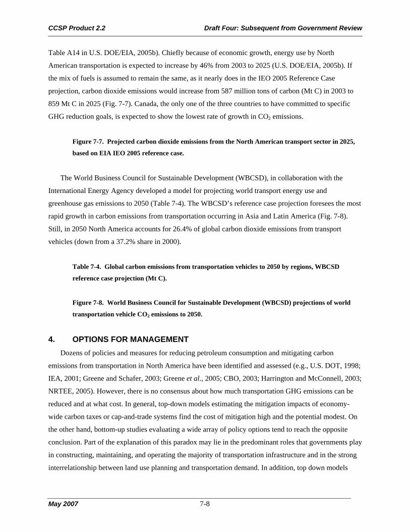
CCSP Product 2.2 Draft Four: Subsequent from Government Review
May 2007 7-8
Table A14 in U.S. DOE/EIA, 2005b). Chiefly because of economic growth, energy use by North
American transportation is expected to increase by 46% from 2003 to 2025 (U.S. DOE/EIA, 2005b). If
the mix of fuels is assumed to remain the same, as it nearly does in the IEO 2005 Reference Case
projection, carbon dioxide emissions would increase from 587 million tons of carbon (Mt C) in 2003 to
859 Mt C in 2025 (Fig. 7-7). Canada, the only one of the three countries to have committed to specific
GHG reduction goals, is expected to show the lowest rate of growth in CO2 emissions.
Figure 7-7. Projected carbon dioxide emissions from the North American transport sector in 2025,
based on EIA IEO 2005 reference case.
The World Business Council for Sustainable Development (WBCSD), in collaboration with the
International Energy Agency developed a model for projecting world transport energy use and
greenhouse gas emissions to 2050 (Table 7-4). The WBCSD’s reference case projection foresees the most
rapid growth in carbon emissions from transportation occurring in Asia and Latin America (Fig. 7-8).
Still, in 2050 North America accounts for 26.4% of global carbon dioxide emissions from transport
vehicles (down from a 37.2% share in 2000).
Table 7-4. Global carbon emissions from transportation vehicles to 2050 by regions, WBCSD
reference case projection (Mt C).
Figure 7-8. World Business Council for Sustainable Development (WBCSD) projections of world
transportation vehicle CO2 emissions to 2050.
4. OPTIONS FOR MANAGEMENT Dozens of policies and measures for reducing petroleum consumption and mitigating carbon
emissions from transportation in North America have been identified and assessed (e.g., U.S. DOT, 1998;
IEA, 2001; Greene and Schafer, 2003; Greene et al., 2005; CBO, 2003; Harrington and McConnell, 2003;
NRTEE, 2005). However, there is no consensus about how much transportation GHG emissions can be
reduced and at what cost. In general, top-down models estimating the mitigation impacts of economy-
wide carbon taxes or cap-and-trade systems find the cost of mitigation high and the potential modest. On
the other hand, bottom-up studies evaluating a wide array of policy options tend to reach the opposite
conclusion. Part of the explanation of this paradox may lie in the predominant roles that governments play
in constructing, maintaining, and operating the majority of transportation infrastructure and in the strong
interrelationship between land use planning and transportation demand. In addition, top down models

CCSP Product 2.2 Draft Four: Subsequent from Government Review
May 2007 7-9
typically assume that all markets are efficient, whereas there is evidence of real-world transportation
energy market failures, especially with respect to the determination of light-duty vehicle fuel economy
(e.g., Turrentine and Kurani, 2004; Chapter 5 in NAS, 2002). Estimates of the costs and benefits of
mitigation policies also vary widely and depend critically on premises concerning (1) the efficiency of
transportation energy markets, (2) the values consumers attach to vehicle attributes such as acceleration
performance and vehicle weight, and (3) the current and future status of carbon-related technology.
A U.S. Energy Information Administration evaluation of a greenhouse gas cap and trade system,
expected to result in carbon permit prices of $79/t C in 2010 and $221/t C in 2025, was estimated to
reduce 2025 transportation energy use by 4.3 PJ and to cut transportation’s carbon emissions by 10%
from 225 Mt C in the reference case to 203 Mt C under this policy (U.S. DOE/EIA, 2003). The average
fuel economy of new light-duty vehicles was estimated to increase from 26.4 mpg (8.9 L per 100 km) to
29.0 mpg (8.1 L per 100 km) in the policy case, an improvement of only 10%. A 2002 study by the U.S.
National Academy of Sciences (NAS, 2002) estimated that “cost-efficient” fuel economy improvements
for United States light-duty vehicles using proven technologies ranged from 12% for subcompact cars to
27% for large cars, and from 25% for small SUVs to 42% for large SUVs. The NAS study did not include
the potential impacts of diesel or hybrid vehicle technologies and assumed that vehicle size and
horsepower would remain constant.
The U.S. Congressional Budget Office (CBO, 2003) estimated that achieving a 10% reduction in
United States gasoline use would create total economic costs of approximately $3.6 billion per year if
accomplished by means of Corporate Average Fuel Economy (CAFE) standards, $3.0 billion if the same
standards allowed trading of fuel economy credits among manufacturers, and $2.9 billion if accomplished
via a tax on gasoline. This partial equilibrium analysis assumed that it would take about 14 years for the
policies to have their full impact. If one assumes that the United States would consume 22,600 PJ of
gasoline in 2017, resulting in 387 Mt of CO2 emissions, then a 10% reduction amounts to 39 Mt C. At a
total cost of $3 billion per year, and attributing the full cost to carbon reduction (vs. other objectives such
as reducing petroleum dependence) produces an upper-bound mitigation cost estimate of $77/t C.
The bipartisan National Commission on Energy Policy (NCEP, 2004) surveyed recent assessments of
the potential to increase light-duty vehicle fuel economy in the United States Taking into consideration
uncertainties about the costs and technical potential of fuel economy technologies, as well as the future
price of fuel, the Commission concluded that future increases in fuel economy of from 40% to 80% could
be achieved at a cost that would be fully offset by the value of fuel saved over the life of a vehicle. They
estimated that the essentially costless carbon emissions reductions would amount to between 250 and 400
million metric tons per year by 2030.

CCSP Product 2.2 Draft Four: Subsequent from Government Review
May 2007 7-10
Systems of progressive vehicle taxes on purchases of less efficient new vehicles and subsidies for
more efficient new vehicles (“feebates”) are yet another alternative for increasing vehicle fuel economy.
A study of the United States market (Greene et al., 2005) examined a variety of feebate structures under
two alternative assumptions: (1) consumers consider only the first three years of fuel savings when
making new vehicle purchase decisions, and (2) consumers consider the full discounted present value of
lifetime fuel savings. The study found that if consumers consider only the first three years of fuel savings,
then a feebate of $1000 per 0.01 gal/mile (3.5 L per 100 km), designed to produce no net revenue to the
government, would produce net benefits to society in terms of fuel savings and would reduce carbon
emissions by 139 Mt C in 2030. If consumers fully valued lifetime fuel savings, the same feebate system
would cause a $3 billion loss in consumers’ surplus (a technical measure of the change in economic well-
being closely approximating income loss) and reduce carbon emissions by only 67 Mt C, or an implied
cost of $44/Mt CO2.
The most widely proposed options for reducing the carbon content of transportation fuels are liquid
fuels derived from biomass and hydrogen produced from renewables, nuclear energy, or from fossil fuels
with carbon sequestration. Biomass fuels, such as ethanol from cellulosic feedstocks or liquid
hydrocarbon fuels produced via biomass gasification and synthesis, appear to be a promising mid- to
long-term option, while hydrogen could become an important energy carrier but not before 2025
(WBCSD, 2004). The carbon emission reduction potential of biomass fuels for transportation is strongly
dependent on the feedstock and conversion processes. Advanced methods of producing of ethanol from
grain, the predominant feedstock in the United States can reduce carbon emissions by 10% to 30%
(Wang, 2005; p. 16 in IEA, 2004). Production of ethanol from sugar cane, as is the current practice in
Brazil, or by not-yet-commercialized methods of cellulosic conversion can achieve up to a 90% net
reduction over the fuel cycle. Conversion of biomass to liquid hydrocarbon fuels via gasification and
synthesis may have a similar potential (Williams, 2005). The technical potential for liquid fuels
production from biomass is very large and very uncertain; recent estimates of the global potential range
from 10 to 400 exajoules per year (see Table 6.8 in IEA, 2004). The U.S. Departments of Energy and
Agriculture have estimated that 30% of United States petroleum use could be replaced by biofuels by
2030 (Perlack et al., 2005). The economic potential will depend on competition for land with other uses,
the development of a global market for biofuels, and advances in conversion technologies.
Hydrogen must be considered a long-term option because of the present high cost of fuel cells,
technical challenges in hydrogen storage, and the need to construct a new infrastructure for hydrogen
production and distribution (NAS, 2004; U.S. DOE, 2005; IEA, 2005b). Hydrogen’s potential to mitigate
carbon emissions from transport will depend most strongly on how hydrogen is produced. If produced
from coal gasification without sequestration of CO2 emissions in production, it is conceivable that carbon

CCSP Product 2.2 Draft Four: Subsequent from Government Review
May 2007 7-11
emissions could increase. If produced from fossil fuels with sequestration, or from renewable or nuclear
energy, carbon emissions from road and rail vehicles could be virtually eliminated (General Motors et al.,
2001).
In a comprehensive assessment of opportunities to reduce GHG emissions from the United States
transportation sector, a study published by the Pew Center on Global Climate Change (Greene and
Schafer, 2003) estimated that sector-wide reductions in the vicinity of 20% could be achieved by 2015
and 50% by 2030 (Table 7-5). The study’s premises assumed no change in the year 2000 distribution of
energy use by mode. A wide range of strategies was considered, including research and development,
efficiency standards, use of biofuels and hydrogen, pricing policies to encourage efficiency and reduce
travel demand, land-use transportation planning options, and public education (Table 7-5). Other key
premises of the analysis were that (1) for efficiency improvements the value of fuel saved to the consumer
must be greater than or equal to the cost of the improvement, (2) there is no change in vehicle size or
performance, (3) pricing policies shift the incidence but do not increase the overall cost of transportation,
and (4) there is a carbon cap and trade system in effect equivalent to a charge of approximately $50/t C.
Similar premises underlie the 2030 estimates, except that technological progress is assumed to have
expanded the potential for efficiency improvement and lowered the cost of biofuels.
Table 7-5. Potential impacts of transportation GHG reduction policies in the United States by 2015
and 2030 based on the 2000 distribution of emissions by mode and fuel.
The Pew Center study notes that if transportation demand continues to grow as the IEO 2005 and
WBCSD projections anticipate, the potential reductions shown in Table 7.4 would be just large enough to
hold United States transportation CO2 emissions in 2030 to 2000 levels.
A study for the U.S. Department of Energy (ILWG, 2000) produced estimates of carbon mitigation
potential for the entire United States economy using a variety of policies generally consistent with carbon
taxes of $25-$50/t C. In the study’s business as usual case, transportation CO2 emissions increased from
478 Mt C in 1997 to 700 Mt C in 2020. A combination of technological advances, greater use of biofuel,
fuel economy standards, paying for a portion of automobile insurance as a surcharge on gasoline, and
others, were estimated to reduce 2020 transportation CO2 emissions by 155 Mt C to 545 Mt CO2. The
study did not produce cost estimates and did not consider impacts on global energy markets.
A joint study of the U.S. Department of Energy and Natural Resources Canada (Patterson et al.,
2003) considered alternative scenarios of highway energy use in the two countries to 2050. The study did
not produce estimates of cost-effectiveness for greenhouse gas reduction strategies but rather focused on
the potential impacts of differing social, economic, and technological trends. Two of the scenarios

CCSP Product 2.2 Draft Four: Subsequent from Government Review
May 2007 7-12
describe paths that lead to essentially constant greenhouse gas emissions from highway vehicles through
2050 through greatly increased efficiency and biofuel and hydrogen use and, in one scenario, reduced
demand for vehicle travel.
5. INCONSISTENCIES AND UNCERTAINTIES There are some inconsistencies in the way the three North American countries report transportation
carbon emissions. The principal source for Mexican emissions data breaks out transportation into four
modes (road, air, rail and waterborne), does not report emissions for pipelines but does report emissions
from use of international bunker fuels. The United States and Canada report transport emissions in much
greater modal detail, by vehicle type and fuel type within modes. The United States and Mexico report
emissions from international bunker fuels in their national inventory reports while Canada does not.
Estimates of international bunker fuel emissions for Canada presented in this chapter were derived by
subtracting Air and Waterborne emissions reported by Environment Canada (2005) which exclude
international bunker fuels from total air and waterborne emissions as reported by Natural Resources
Canada (2006) which include them. Environment Canada reports off-road emissions from mobile sources
separately; in the tables and figures in this chapter Canadian off-road emissions have been added to road
emissions. Both Canada and the United States include emissions from military transport operations in
their inventories. It is not clear whether these are included in the estimates for Mexico.
All three countries’ greenhouse gas inventories discuss uncertainties in estimated emissions. In
general, the uncertainties were estimated in accordance with IPCC guidelines. The U.S. EPA provides
only an estimate of a 95% confidence interval for all carbon dioxide emissions from the combustion of
fossil fuels (-1% to 6%) which can be inferred to apply to transportation. Mexico’s INE estimates a total
uncertainty for transportation greenhouse gas emissions of about ± 10%. For carbon dioxide emissions
from road transport, the uncertainty is put at ± 9% (INE, 2003, Appendix B). The Canadian Greenhouse
Gas Inventory provides by far the most extensive and detailed estimates of uncertainty. Given the
similarity in methods, the Canadian uncertainty estimates are probably also approximately correct for the
United States, and therefore may be considered indicative of the uncertainty of North American carbon
emission estimates (Table 7-6). Most significant is the apparent overestimation of carbon emissions from
on-road vehicles, offset to a degree by the underestimation of off-road mobile source emissions. Still,
total mobile source carbon emissions are estimated to have a 95% confidence interval of (-4% to 0%).
Table 7-6. Uncertainty in estimates of carbon dioxide emissions from energy use in transport: Canada
2003.

CCSP Product 2.2 Draft Four: Subsequent from Government Review
May 2007 7-13
6. RESEARCH AND DEVELOPMENT NEEDS Research needs with respect to the transport sector as a part of the carbon cycle fall into three
categories: (1) improved data, (2) comprehensive assessments of mitigation potential, and (3) advances in
key mitigation technologies and policies for transportation. The available data are adequate to describe
carbon inputs by fuel type and carbon emissions by very broad modal breakdowns by country.
Environment Canada (2005) and the U.S. Environmental Protection Agency (2005) annually publish
estimates of transportation’s carbon emissions that closely follow IPCC guidelines with respect to
methods, data sources and quantification of uncertainties (GAO, 2003). The Mexican Instituto Nacional
de Ecología has published estimates for 2001 that are also based on IPCC methods. However, that report
also notes deficiencies in the data available for Mexico’s transport sector and recommends establishing an
information system for estimating Mexico’s transportation’s greenhouse gas emissions on a continuing
basis (INE, 2003, p. 21). Knowledge of the magnitudes of GHG emissions by type of activity and fuel
and of trends is essential if policies are to be focused on the most important GHG sources.
The most pressing research need is for comprehensive, consistent, and rigorous assessments of the
carbon emissions mitigation potential for North American transportation. The lack of such studies for
North America parallels a similar dearth of consistent and comprehensive global analyses noted by the
Intergovernmental Panel on Climate Change (Moomaw and Moreira, 2001). Existing studies focus almost
exclusively on a single country, with premises and assumptions varying widely from country to country.
Even the best single country studies omit the impacts of carbon reduction policies on global energy
markets. Knowledge of how much contribution the transport sector can make to GHG mitigation at what
cost and what options are capable of achieving those potentials is crucial to the global GHG policy
discussion.
Continued research and development of vehicle technologies and fuels that can cost-effectively
increase energy efficiency and displace carbon-based fuels is essential to achieving major reductions in
transportation carbon emissions. Highly promising technologies for reducing transportation GHG
emissions include hybrid vehicles, which are available today, and in the future, plug-in hybrid vehicles
capable of accepting electrical energy from the grid, and eventually fuel cell vehicles powered by
hydrogen. While hybrids are already in the market and fuel cell vehicles are still years away, all three
technologies would benefit from cost reduction. Hydrogen fuel cell vehicles also face significant
technological challenges with respect to hydrogen storage and fuel cell durability. Energy-efficient
technologies could also greatly reduce greenhouse gas emissions from other transport modes. For
example, blended wing-body aircraft designs are under development that could reduce fuel burn rates by
one-third. Biofuels in the near term and hydrogen in the longer term appear to be the most promising low-
carbon fuel options. To achieve the greatest greenhouse gas reduction benefits, biofuels must be made

CCSP Product 2.2 Draft Four: Subsequent from Government Review
May 2007 7-14
from plants’ lingo-cellulosic components either by conversion to alcohol or by gasification and synthesis
of liquid hydrocarbon fuels. Cost reductions in both feedstock production and fuel conversion are needed.
CHAPTER 7 REFERENCES CBO (Congressional Budget Office), 2003: The Economic Costs of Fuel Economy Standards Versus a Gasoline
Tax. Congress of the United States, Washington, DC, December.
CIA (Central Intelligence Agency), 2005: The World Factbook. Washington, DC, November 8. Available at
http://www.cia.gov/cia/publications/factbook
Davis, S.C. and S.W. Diegel, 2004: Transportation Energy Data Book: Edition 24. ORNL-6973, Oak Ridge
National Laboratory, Oak Ridge, TN.
Environment Canada, 2005: Canada’s Greenhouse Gas Inventory: 1990-2003. National Inventory Report, Ottawa,
Ontario, Canada.
Fulton, L. and G. Eads, 2004: IEA/SMP Model Documentation and Reference Case Projection. World Business
Council for Sustainable Development. Available at http://www.wbcsd.ch/web/publications/mobility/smp-
model-document.pdf, July.
GAO (United States General Accounting Office), 2003: Climate Change, Selected Nations’ Reports on Greenhouse
Gas Emissions Varied in Their Adherence to Standards. GAO-04-98, Washington, DC, December. Available at
http://www.gao.gov/cgi-bin/getrpt?GAO-04-98.
General Motors Corporation, Argonne National Laboratory, ExxonMobil, and Shell, 2001: Well-to-Wheel Energy
Use and Greenhouse Gas Emissions of Advanced Fuel/Vehicle Systems: North American Analysis. Vol. 2,
Argonne National Laboratory, Argonne, IL, June.
Government of Canada, 2005. Moving Forward on Climate Change: A Plan for Honouring our Kyoto
Commitment. Ottawa, Canada. Available at http://www.climatechange.gc.ca
Greene, D.L. and A. Schafer, 2003: Reducing Greenhouse Gas Emissions from U.S. Transportation. Pew Center on
Global Climate Change, Arlington, VA, May.
Greene, D.L., P.D. Patterson, M. Singh, and J. Li, 2005: Feebates, rebates and gas-guzzler taxes: a study of
incentives for increased fuel economy. Energy Policy, 33(6), 757-776.
Harrington, W. and V. McConnell, 2003: Motor Vehicles and the Environment. RFF Report, Resources for the
Future, Washington, DC, April.
IEA (International Energy Agency), 2005a: World Energy Outlook 2005. OECD, Paris, France.
IEA (International Energy Agency), 2005b: Prospects for Hydrogen and Fuel Cells. OECD, Paris, France.
IEA (International Energy Agency), 2004: Biofuels for Transport. OECD, Paris, France.
IEA (International Energy Agency), 2001: Saving Oil and Reducing CO2 Emissions in Transport. OECD, Paris,
France.
ILWG (Interlaboratory Working Group), 2000: Scenarios for a Clean Energy Future. Prepared by Lawrence
Berkeley National Laboratory (LBNL-44029) and Oak Ridge National Laboratory (ORNL/CON-476) for the
U.S. Department of Energy.

CCSP Product 2.2 Draft Four: Subsequent from Government Review
May 2007 7-15
INE (Instituto Nacional de Ecología), 2003: Energía. Sector Transporte 2000-2001, Inventario Nacional de
Emisiones de Gases de Efecto Invernadero, INGEI/2000/ENC, Mexico D.F. Available at
http://www.ine.gob.mx/dgicurg/cclimatico/inventario.html
Marland, G., T. Boden, and R.J. Andres, 2005: Global CO2 Emissions from Fossil Fuel Burning, Cement
Manufacture and Gas Flaring, 1751-2002. Available at
http://cdiac.esd.ornl.gov/ftp/ndp030/global.1751_2002.ems, November 8.
Moomaw, W.R. and J.R. Moreira, 2001: Technological and economic potential of greenhouse gas emissions
reduction (Chapter 3). In: Climate Change 2001: Mitigation [Metz, Davidson, Swart, and Pan (eds.)].
Cambridge University Press, Cambridge, UK.
Nakićenović, N., A. Grűbler, and A. McDonald, 1998: Global Energy Perspectives. Cambridge University Press,
Cambridge, UK.
NAS (National Academy of Sciences), 2004: The Hydrogen Economy. National Academies Press, Washington, DC.
NAS (National Academy of Sciences), 2002: Effectiveness and Impact of Corporate Average Fuel Economy
(CAFE) Standards. National Academies Press, Washington, DC.
NATS (North American Transportation Statistics), 2005: Various Tables. A joint project of the U.S. Bureau of
Transportation Statistics, Statistics Canada and Instituto Nacional de Estadistica Gegrafica Informatica
(INEGI), Mexico. Available at http://nats.sct.gob.mx/lib/series
NCEP (National Commission on Energy Policy), 2004: Ending the Energy Stalemate, A Bipartisan Strategy to Meet
America’s Energy Challenges, Chapter 3, Washington, D.C.: National Commission on Energy Policy.
Available at www.energycommission.org
NRCan (Natural Resources Canada), 2006: Comprehensive Energy Use Database Tables. Transportation sector,
table 1: secondary energy use by source, table 8: GHG emissions by transportation mode. Available at
http://oee.nrcan.gc.ca/corporate/statistics/neud/dpa/trends_tran_ca.cfm
NRTEE (National Round Table on the Environment and the Economy), 2005: Economic Instruments for Long-
term Reductions in Energy-based Carbon Emissions. Renouf Publishing Co., Ltd., Ottawa, Ontario, Canada.
Patterson, P., D. Greene, E. Steiner, S. Plotkin, M. Singh, A. Vyas, M. Mintz, D. Santini, S. Folga, J. Moore, P.
Reilly-Roe, K. Cliffe, R. Talbot, P. Khannna, and V. Stanciulescu, 2003: Joint DOE/NRCan Study of North
American Transportation Energy Futures. Energy Efficiency and Renewable Energy, U.S. Department of
Energy, Washington, DC, May. Available at www.eere.energy.gov/ba/pdfs/final_2050_pres.pdf
Perlack, R.D., L.L. Wright, A.F. Turhollow, R.L. Graham, B.J. Stokes, and D.C. Erbach, 2005: Biomass as
Feedstock for a Bioenergy and Bioproducts Industry: The Technical Feasibility of a Billion-Ton Annual Supply.
DOE/GO-102995-2135, U.S. Department of Energy, Washington, DC, April.
Rodriíguez, H.M., 2005: Perspectivas del Uso de los Hidrocarburos a Nevel México. Presentation, Subsecretario
de Hidrocarburos, Mexico City, Mexico, April 14.
SENER (Secretaria de Energia), 2005: Sistema de Información Energetica, información estadistica. Available at
http://sie.energia.gob.mx/sie, under Consumo final de energia en el sector transporte.

CCSP Product 2.2 Draft Four: Subsequent from Government Review
May 2007 7-16
Turrentine, T. and K. Kurani, 2004: Automotive Fuel Economy in the Purchase and Use Decisions of Households.
ITS-RR-04-31, Institute for Transportation Studies, University of California at Davis, Davis, CA, September.
U.S. DOE (U.S. Department of Energy), 2005: Hydrogen, Fuel Cells and Infrastructure Technologies Program:
Multi-Year Research, Development and Demonstration Plan. DOE/GO-102003-1741, Energy Efficiency and
Renewable Energy. Available at www.eere.energy.gov, January.
U.S. DOE/EIA (U.S. Department of Energy, Energy Information Administration), 2005a: Annual Energy Review
2004. DOE/EIA-0384(2004), Washington, DC, August. Available at www.eia.doe.gov
U.S. DOE/EIA (U.S. Department of Energy, Energy Information Administration), 2005b: International Energy
Outlook 2005. DOE/EIA-0484(2005), Washington, DC.
U.S. DOE/EIA (U.S. Department of Energy, Energy Information Administration), 2003: Analysis of S.139, the
Climate Stewardship Act of 2003. SR/OIAF/2003-02, Washington, DC, June.
U.S. DOT (U.S. Department of Transportation), 1998: Transportation and Global Climate Change: A Review and
Analysis of the Literature. Federal Highway Administration, Washington, DC, June.
U.S. EPA (U.S. Environmental Protection Agency), 2005: Inventory of U.S. Greenhouse Gas Emissions and Sinks:
1990-2003. EPA 430-R-05-003, Office of Atmospheric Programs, Washington, DC, April 15.
Wang, M.Q., 2005: Argonne Expert Addresses Energy and Environmental Impacts of Fuel Ethanol. TransForum,
5(2), Transportation Technology R&D Center, Argonne National Laboratory, Argonne, IL, November.
Weiss, M.A., J.B. Heywood, E.M. Drake, A. Schafer, and F.F. AuYeung, 2000: On the Road in 2020. Energy
Laboratory Report #MIT EL 00-003, Energy Laboratory, Massachusetts Institute of Technology, Cambridge,
MA, October.
Williams, R.H., 2005: CO2 Capture and Storage Strategies for Coal and Biomass to Reduce GHG Emissions for
Synfuels. Princeton Environmental Institute, Princeton University, Princeton, NJ, March.
WBCSD (World Business Council for Sustainable Development), 2004: Mobility 2030. The Sustainable Mobility
Project, Geneva, Switzerland. Available at www.wbcsd.org

CCSP Product 2.2 Draft Four: Subsequent from Government Review
May 2007 7-17
Table 7-1. Carbon emissions from transportation in North America in 2003
North American Carbon Emissions by Country and Mode, 2003/2001 (Mt C)
U.S.A. Canada Mexico North America 2003 2003 2001 2003/2001 Road 399.4 36.7 26.0 462.0 Domestic Air 46.7 1.9 1.8 50.4 Rail 11.7 1.4 0.4 13.5 Domestic Water 15.7 1.6 0.9 18.1 Pipeline 9.5 2.4 11.9 International Bunker 23.0 3.0 0.5 26.4 Off-Road 4.6 4.6 Total 505.9 51.7 29.4 587.0 Sources: U.S. EPA, 2005; Environment Canada, 2005; INE, 2003. Note: Data for Mexico is 2001, U.S.A. and Canada are 2003. Carbon dioxide emissions estimates are considered by the Canadian and Mexican sources to have 95% certainty that the actual value is within 10% of the estimate reported. The United States did not provide quantitative uncertainty estimates for 2003, but these estimates are considered to be equally accurate by the author.

CCSP Product 2.2 Draft Four: Subsequent from Government Review
May 2007 7-18
Table 7-2. Summary of North American transport energy use and carbon dioxide emissions
in 2003 by energy source or fuel type
North America energy source
Energy input
(Petajoules)
Carbon input
(Mt C)
Gasoline 20,923 358.3 Diesel/distillate 7,344 129.5 Jet fuel/kerosene 2,298 68.5 Residual 681 14.5 Other fuels 124 1.3 Natural gas 926 9.7 Electricity 36 0.0 Unalloc./error 466 - Total 32,798 581.8 United States
Gasoline 18,520 312.5 Diesel/distillate 6,193 107.1 Jet fuel/kerosene 1,986 62.3 Residual 612 13.1 Other fuels 50 0.2 Natural gas 748 9.7 Electricity 20 0.0 Unalloc./error 466.2 -
Total 28,595.2 504.9 Sources: U.S. EPA, 2005, Tables 3-7 and 2-17; Davis and Diegel, 2004, Tables 2.6 and 2.7. Canada
Gasoline 1,355 26.2 Diesel/distillate 698 13.9 Jet fuel/kerosene 223 4.3 Residual 67 1.3 Other fuels 17 0.2 Natural gas 2 0.0 Electricity 3 0.0 Unalloc./error 0
Total 2,363 45.9 NRCan, 2006, Tables 1 and 8. Mexico
Gasoline 1,066 19.5 Diesel/distillate 447 8.5 Jet fuel/kerosene 106 1.9 Residual 4 0.1 Other fuels 57 0.9 Natural gas 1 0.0 Electricity 4 0.0 Unalloc./error
Total 1,685 31.0 Sources: Transportation energy use by fuel and mode from Rodriguez, 2005.

CCSP Product 2.2 Draft Four: Subsequent from Government Review
May 2007 7-19
Source: Fulton and Eads, 2004, spreadsheet model, output worksheet. The accuracy of the data in the above table is judged by the author to be 95% certain that the actual value is within 10% of the estimate reported.
Data sources differ somewhat by country with respect to modal, fuel, and greenhouse gas definitions so that the numbers are not precisely comparable. Canadian carbon emissions data include all greenhouse gases produced by transportation in CO2 equivalents, while the United States data are CO2 emissions only. Carbon dioxide emissions for Mexico were estimated by applying U.S. EPA emissions factors to the Mexican energy use data. For Mexico, it is assumed that no transportation carbon emissions result from electricity use.
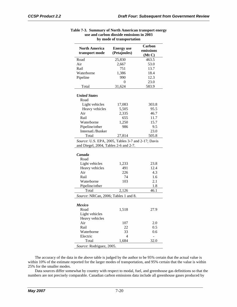
CCSP Product 2.2 Draft Four: Subsequent from Government Review
May 2007 7-20
Table 7-3. Summary of North American transport energy use and carbon dioxide emissions in 2003
by mode of transportation
North America transport mode
Energy use (Petajoules)
Carbon emissions
(Mt C) Road 25,830 463.5 Air 2,667 53.0 Rail 751 13.7 Waterborne 1,386 18.4 Pipeline 990 12.3 0 23.0 Total 31,624 583.9 United States
Road Light vehicles 17,083 303.8 Heavy vehicles 5,505 95.5 Air 2,335 46.7 Rail 655 11.7 Waterborne 1,250 15.7 Pipeline/other 986 9.5 Internatl./Bunker 23.0
Total 27,814 505.8 Source: U.S. EPA, 2005, Tables 3-7 and 2-17; Davis and Diegel, 2004, Tables 2-6 and 2-7. Canada
Road Light vehicles 1,233 23.8 Heavy vehicles 491 12.4 Air 226 4.3 Rail 74 1.6 Waterborne 103 2.1 Pipeline/other 1.8 Total 2,126 46.1
Source: NRCan, 2006; Tables 1 and 8. Mexico
Road 1,518 27.9 Light vehicles Heavy vehicles Air 107 2.0 Rail 22 0.5 Waterborne 33 0.6 Electric 4 - Total 1,684 32.0
Source: Rodriguez, 2005.
The accuracy of the data in the above table is judged by the author to be 95% certain that the actual value is within 10% of the estimate reported for the larger modes of transportation, and 95% certain that the value is within 25% for the smaller modes.
Data sources differ somewhat by country with respect to modal, fuel, and greenhouse gas definitions so that the numbers are not precisely comparable. Canadian carbon emissions data include all greenhouse gases produced by

CCSP Product 2.2 Draft Four: Subsequent from Government Review
May 2007 7-21
transportation in CO2 equivalents, while the United States data are CO2 emissions only. Carbon dioxide emissions for Mexico were estimated by applying U.S. EPA emissions factors to the Mexican energy use data. Electricity is assumed to produce no carbon emissions in end use.
Table 7-4. Global carbon emissions from transportation vehicles to 2050 by regions, WBCSD reference case projection (Mt C)
2000 2010 2020 2030 2040 2050 OECD North America 544 623 708 768 824 882 OECD Europe 313 359 392 412 420 428 OECD Pacific 133 142 153 161 169 179 FSU 48 64 88 109 132 153 Eastern Europe 23 28 36 42 52 66 China 69 108 163 225 308 417 Other Asia 98 131 174 220 283 368 India 38 54 80 108 146 203 Middle East 59 71 88 106 122 138 Latin America 95 127 172 216 275 352 Africa 43 58 80 103 127 158 TOTAL - All Regions 1463 1766 2134 2470 2858 3343
Source: Fulton and Eads, 2004.
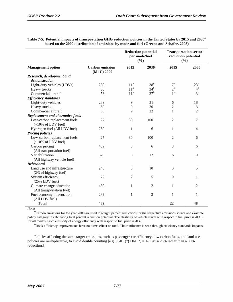
CCSP Product 2.2 Draft Four: Subsequent from Government Review
May 2007 7-22
Table 7-5. Potential impacts of transportation GHG reduction policies in the United States by 2015 and 2030a based on the 2000 distribution of emissions by mode and fuel (Greene and Schafer, 2003)
Reduction potential per mode/fuel
(%)
Transportation sector reduction potential
(%)
Management option Carbon emission (Mt C) 2000
2015 2030 2015 2030
Research, development and demonstration
Light-duty vehicles (LDVs) 289 11b 38b 7b 23b Heavy trucks 80 11b 24b 2b 4b Commercial aircraft 53 11b 27b 1b 3b
Efficiency standards Light-duty vehicles 289 9 31 6 18 Heavy trucks 80 9 20 2 3 Commercial aircraft 53 9 22 1 2
Replacement and alternative fuels Low-carbon replacement fuels (~10% of LDV fuel)
27 30 100 2 7
Hydrogen fuel (All LDV fuel) 289 1 6 1 4 Pricing policies
Low-carbon replacement fuels (~10% of LDV fuel)
27 30 100 2 6
Carbon pricing (All transportation fuel)
489 3 6 3 6
Variabilization (All highway vehicle fuel)
370 8 12 6 9
Behavioral Land use and infrastructure (2/3 of highway fuel)
246 5 10 3 5
System efficiency (25% LDV fuel)
72 2 5 0 1
Climate change education (All transportation fuel)
489 1 2 1 2
Fuel economy information (All LDV fuel)
289 1 2 1 1
Total 489 22 48 Notes:
aCarbon emissions for the year 2000 are used to weight percent reductions for the respective emissions source and example policy category in calculating total percent reduction potential. The elasticity of vehicle travel with respect to fuel price is -0.15 for all modes. Price elasticity of energy efficiency with respect to fuel price is -0.4.
bR&D efficiency improvements have no direct effect on total. Their influence is seen through efficiency standards impacts.
Policies affecting the same target emissions, such as passenger car efficiency, low carbon fuels, and land use policies are multiplicative, to avoid double counting [e.g. (1-0.1)*(1.0-0.2) = 1-0.28, a 28% rather than a 30% reduction.]

CCSP Product 2.2 Draft Four: Subsequent from Government Review
May 2007 7-23
Table 7-6. Uncertainty in estimates of carbon dioxide emissions from energy use in transport: Canada 2003
Mode
% Below
(2.5th Percentile)
% Above
(97.5th Percentile)
Total Mobile Sources excluding pipeline -4 0 Road Transportation -8 -3 On-Road Gasoline Vehicles -7 -3 On-Road Diesel Vehicles -13 -1 Railways -5 3 Navigation -3 3 Off-Road Mobile Sources 4 45 Pipeline -3 3
Source: Environment Canada, 2005, table A7-9.
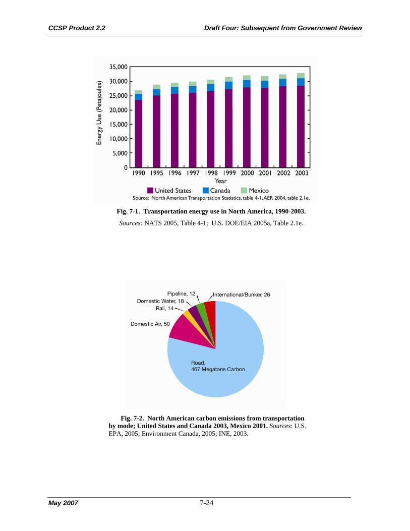
CCSP Product 2.2 Draft Four: Subsequent from Government Review
May 2007 7-24
Fig. 7-1. Transportation energy use in North America, 1990-2003.
Sources: NATS 2005, Table 4-1; U.S. DOE/EIA 2005a, Table 2.1e.
Fig. 7-2. North American carbon emissions from transportation
by mode; United States and Canada 2003, Mexico 2001. Sources: U.S. EPA, 2005; Environment Canada, 2005; INE, 2003.

CCSP Product 2.2 Draft Four: Subsequent from Government Review
May 2007 7-25
Fig. 7-3A. Freight activity by mode in Canada. Source: NATS 2005, Table 5-2.
Fig. 7-3B. Freight activity by mode in Mexico. Source: NATS 2005, Table 5-2.

CCSP Product 2.2 Draft Four: Subsequent from Government Review
May 2007 7-26
Fig. 7-3C. Freight activity by mode in the United States. Source: NATS 2005, Table 5-2.
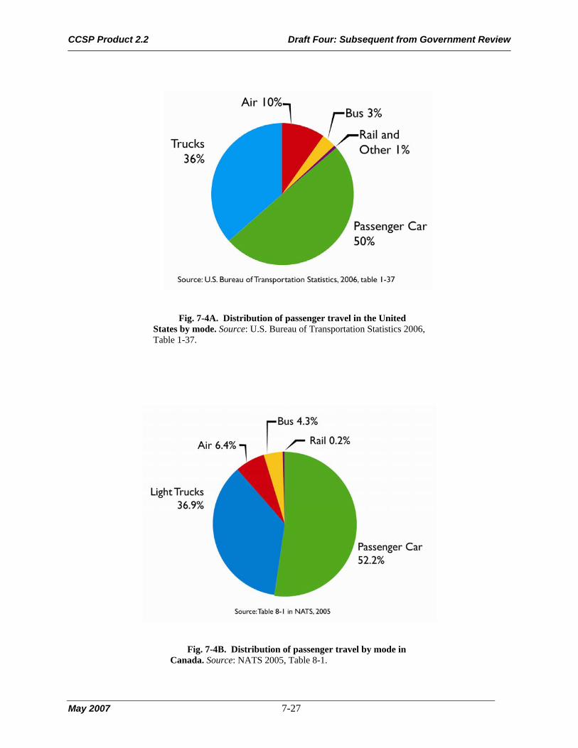
CCSP Product 2.2 Draft Four: Subsequent from Government Review
May 2007 7-27
Fig. 7-4A. Distribution of passenger travel in the United States by mode. Source: U.S. Bureau of Transportation Statistics 2006, Table 1-37.
Fig. 7-4B. Distribution of passenger travel by mode in Canada. Source: NATS 2005, Table 8-1.

CCSP Product 2.2 Draft Four: Subsequent from Government Review
May 2007 7-28
Fig. 7-5A. Evolution of transport energy use in Mexico. Source: SENER 2005.
Fig. 7-5B. Evolution of transport energy use in the United States.
Source: Davis and Diegel 2004, Tables 2.6 and 2.7.

CCSP Product 2.2 Draft Four: Subsequent from Government Review
May 2007 7-29
Fig. 7-6A. Transport CO2 emissions in Canada. Source: NRCan 2006.
Fig. 7-6B. Transport CO2 emissions in the United States. Source: U.S. EPA 2005, Table 2-17.
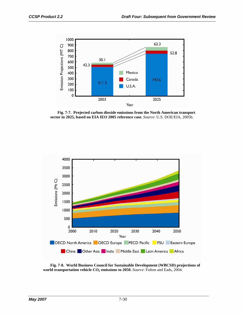
CCSP Product 2.2 Draft Four: Subsequent from Government Review
May 2007 7-30
Fig. 7-7. Projected carbon dioxide emissions from the North American transport
sector in 2025, based on EIA IEO 2005 reference case. Source: U.S. DOE/EIA, 2005b.
Fig. 7-8. World Business Council for Sustainable Development (WBCSD) projections of
world transportation vehicle CO2 emissions to 2050. Source: Fulton and Eads, 2004.

CCSP Product 2.2 Draft Four: Subsequent from Government Review
May 2007 8-1
Chapter 8. Industry and Waste Management
Lead Author: John Nyboer1
Contributing Authors: Mark Jaccard2 and Ernst Worrell3
1Canadian Industrial Energy End-Use Data and Analysis Centre (CIEEDAC), Simon Fraser University,
2Simon Fraser University, 3Lawrence Berkeley National Laboratory
KEY FINDINGS
• In 2002, North America’s industry (not including fossil-fuel mining and processing or electricity
generation) contributed 225 Mt C (826 Mt CO2), 16% of the world’s carbon dioxide emissions to
the atmosphere from industry. Waste treatment plants and landfill sites in North America
accounted for 13.4 Mt of methane (282 Mt CO2 equivalent; 10 Mt C), roughly 20% of global totals.
• Industrial carbon dioxide emissions from North America decreased nearly 11% between 1990
and 2002, while energy consumption in the United States and Canada increased 8% to 10%
during that period. In both countries, a shift in production activity toward less energy-intensive
industries and dissemination of more energy efficient equipment kept the rate of energy demand
growth lower than industrial Gross Domestic Product growth.
• Changes in industrial carbon dioxide emissions are a consequence of changes in industrial
energy demand and changes in the mix of fossil fuels used by industry to supply that demand.
Changes in industrial energy demand are themselves a consequence of changes in total
industrial output, shifts in the relative shares of industrial sectors, and increases in energy
efficiency. Shifts from coal and refined petroleum products to natural gas and electricity
contributed to a decline in total industrial carbon dioxide emissions since 1997 in both Canada
and the United States.
• An increase in carbon dioxide emissions from North American industry is likely to accompany the
forecasted increase in industrial activity (2.3% per year until 2025 for the United States).
• Emissions per unit of industrial activity will likely decline as non-energy intensive industries grow
faster than energy intensive industries and with increased penetration of energy efficient
equipment. However, continuation of the trend toward less carbon-intensive fuels is uncertain
given the rise in natural gas prices relative to coal in recent years.
• Options for reducing carbon dioxide emissions from North American industry can be broadly
classified as methods to: (1) reduce process/fugitive emissions or convert currently released
emissions; (2) increase energy efficiency, including combined heat and power management; (3)
change industrial processes (materials efficiency, recycling, substitution between materials or

CCSP Product 2.2 Draft Four: Subsequent from Government Review
May 2007 8-2
between materials and energy, nanotechnology); (4) substitute less carbon intense fuels; and (5)
capture and store carbon dioxide.
• Further work on materials substitution holds promise for industrial emissions reduction, such as
the replacement of petrochemical feedstocks by feedstocks derived from vegetative matter
(biomass), of steel by aluminum in the transport sector, and of concrete by wood in the buildings
sector. The prospects for greater usage of energy efficiency technologies, are equally substantial.
1. INTRODUCTION
This chapter assesses carbon flows through industry (manufacturing, construction, including industry
process emissions, but excludes fossil-fuel mining and processing)1 and municipal waste disposal.
In 2002, industry was responsible for 1423.8 million tons of carbon (Mt C) (5220.6 million tons of
carbon dioxide [Mt CO2]), which is 21% of human-caused (anthropogenic) emissions to the atmosphere
(244.8 Mt C [4322.9 Mt CO2] from fuel combustion and 1179.0 Mt C [897.7 Mt CO2] from industrial
processes). North America’s industry contributed 206.9 Mt C (758.7 Mt CO2) of combustion-sourced
emissions and 18.2 Mt C (66.8 Mt CO2) of process emissions for a total of 225 Mt C (826 Mt CO2) or
16% of global totals (WRI, 2005; see Fig. 8-1A).† The manufacturing industry contributed 12% of total
North American greenhouse gas (GHG) emissions, lower than in many other parts of the world. However,
with North America’s population at 6.8% of the world’s total, industry contributed a proportionally larger
share of total industrial emissions per capita than the rest of the world.2
Figure 8-1A. CO2 emissions by sector in 2002.
Industrial CO2 emissions decreased nearly 11% between 1990 and 2002 while energy consumption in
the United States and Canada increased 8% to 10% (EIA, 2005; CIEEDAC, 2005). In both countries, a
shift in production activity toward less energy-intensive industries and dissemination of more energy
efficient equipment kept the rate of growth in energy demand lower than industrial Gross Domestic
Product (GDP) growth (IEA, 2004).3 This slower demand growth, in concert with a shift toward less
carbon-intensive fuels, explains the decrease in industrial CO2 emissions.
† The magnitude and/or range of uncertainty for the given numerical value(s) is not provided in the references cited. 1 This includes direct flows only. Indirect carbon flows (e.g., due to electricity generation) are associated with power
generation. 2 North America, including Mexico, was responsible for about 27% of global CO2 emissions in 2002. 3 Decomposition analyses can assess changes in energy consumption due to, for example, increases in industry activity,
changes in relative productivity to or from more intense industry subsectors, or changes in material or energy efficiency in processes.

CCSP Product 2.2 Draft Four: Subsequent from Government Review
May 2007 8-3
The municipal waste stream excludes agricultural and forestry wastes but includes wastewater.
Carbon dioxide, generated from aerobic metabolism in waste removal and storage processes, arises from
biological material and is considered GHG neutral. Methane (CH4), released from anaerobic activity at
waste treatment plants and landfill sites, forms a substantial portion of carbon emissions to the
atmosphere. Given its high global warming potential (GWP) (i.e., the GWP for methane is 21 times that
of CO2), methane plays an important role in the evaluation of possible climate change impacts (WRI,
2005; see Fig. 8-1B).†4 Globally, CH4 emissions from waste amount to 66 Mt, or 378 Mt C equivalent
(1386 Mt CO2 equivalent). North American activity accounts for 13.4 Mt of CH4 (77 Mt C equivalent
[282 Mt CO2 equivalent]) or roughly 20% of global totals.
Figure 8-1B. GHG emissions by sector in 2000, CO2, CH4, N2O, PFCs, HFCs, and SF6.
Substantial sequestration of carbon occurs in landfills.5 Data on carbon buried there are poor. The
Environmental Protection Agency (EPA), using data from Barlaz and Ham (1990) and Barlaz (1994),
estimated that 30% of carbon in food waste and up to 80% of carbon in newsprint, leaves, and branches
remain in the landfill.† Plastics show no deterioration. In all, 80% of the carbon entering a landfill site
may be sequestered, depending on moisture, aeration, and site conditions. Bogner and Spokas (1993)
estimate that “more than 75% of the carbon deposited in landfills remains in sedimentary storage.”
2. INDUSTRY CARBON CYCLE
Carbon may enter industry as a fuel or as a feedstock where the carbon becomes entrained in the
industry’s final product. Carbon in the waste stream can be distinguished as atmospheric and non-
atmospheric, the former being comprised of process and combustion-related emissions. Process CO2
emissions, a non-combustive source, are the result of the transformation of the material inputs to the
production process. For example, cement production involves the calcination of lime, which chemically
alters limestone to form calcium oxide and releases CO2. Of course, combustion-related CO2 emissions
occur when carbon-based fuels provide thermal energy to drive industrial processes.
2.1 Overview of Carbon Inputs and Outputs
Industry generates about one-third as much emitted carbon as the production of electricity and other
fuel supply in North America and only about 55% as much as is generated by the transportation sector.
4 While not carbon-based, N2O from sewage treatment is included in Fig. 8-4, below, to show its relative GHG importance. 5 IPCC guidelines currently do not address landfill sequestration. Such guidelines will be in the 2006 publication.

CCSP Product 2.2 Draft Four: Subsequent from Government Review
May 2007 8-4
2.1.1 Carbon In
Carbon-based raw materials typically enter industrial sites as biomass (primarily wood), limestone,
soda ash, oil products, coal/coke, natural gas, and natural gas liquids. These inputs are converted to
dimension lumber and other wood products, paper and paperboard, cement and lime, glass, and a host of
chemical products, plastics, and fertilizers.
While the bulk of the input carbon leaves the industrial site as a product, some leaves as process CO2
and some is converted to combustible fuel. Waste wood (or hog fuel) and black liquor, generated in the
production of chemical pulps, are burned to provide process heat or steam for digesting wood chips or for
drying paper or wood products, in some cases providing electricity through cogeneration. Chemical
processes utilizing natural gas often generate off-gases that, mixed with conventional fuels, provide
process heat. Finally, some of the carbon that enters as a feedstock leaves as solid or liquid waste.
In some industries, carbon is used to remove oxygen from other input materials through “reduction.”
In most of the literature, such carbon is considered an input to the process and is released as “process”
CO2, even though it acts as a fuel (i.e., it unites with oxygen to form CO2 and releases heat). For example,
in metal smelting and refining processes, a carbon-based reductant separates oxygen from the metal
atoms. Coke, from the destructive distillation of coal, enters a blast furnace with iron ore to strip off the
oxygen associated with the iron. Carbon anodes in electric arc furnaces in steel mills and specialized
electrolytic “Hall-Heroult” cells oxidize to CO2 as they melt recycled steel or reduce alumina to
aluminum.
2.1.2 Carbon Out
Carbon leaves industry as part of the intended commodity or product, as a waste product or as a gas,
usually CO2.
Process emissions are CO2 emissions that occur as a result of the process itself—the calcining of
limestone releases about 0.5 tons CO2 per ton of clinker (unground cement) or about 0.8 tons per ton of
lime.6,7 The oxidation of carbon anodes generates about 1.5 tons CO2 to produce a ton of aluminum.
Striping hydrogen from methane to make ammonia releases about 1.6 tons CO2 per ton of ammonia.
Combustion of carbon-based fuels results in the emission of CO2. In many cases, the combustion
process is not complete and other carbon-based compounds may be released (carbon monoxide, methane,
volatile organic compounds). These often decompose into CO2, but their life spans in the atmosphere
vary.
6 In these industries, more CO2 is generated from processing limestone than from the fossils fuels combusted. 7 The calcination of limestone also takes place in steel, pulp and paper, glass and sugar industries.

CCSP Product 2.2 Draft Four: Subsequent from Government Review
May 2007 8-5
2.1.3 Carbon Flow
Figure 8-2 illustrates the flows of carbon in and out of industries in North America. Comparable
diagrams for individual countries are presented in Appendix 8A. On the left side of Fig. 8-2, all carbon-
based material by industry sector is accounted for, whether in fuel or in feedstock. On the right, the
exiting arrows portray how much of the carbon leaves as part of the final products from that industry. The
carbon in the fossil fuel and feedstock materials leave in the waste stream as emissions from fuel
combustion (including biomass), as process emissions, or as other products and waste. Carbon capture
and storage potentials are assessed in the industry subsections below.
Figure 8-2. Carbon flows for Canada, the United States, and Mexico combined.
2.2 Sectoral Trends in the Industrial Carbon Cycle
Figure 8-2 shows that energy-intensive industries differ significantly in their carbon cycle dynamics.
2.2.1 Pulp and Paper
While pulp and paper products are quite energy-intensive, much of the energy is obtained from
biomass. By using hog fuel and black liquor, some types of pulp mills are energy self-sufficient. Biomass
fuels are considered carbon neutral because return of the biomass carbon to the atmosphere completes a
cycle that began with carbon uptake from the atmosphere by vegetation.8 Fuel handling difficulties and air
quality concerns can arise from the use of biomass as a fuel.
2.2.2 Cement, Lime, and Other Nonmetallic Minerals
Cement and lime production require the calcination of limestone, which releases CO2; about 0.78 tons
of CO2 per ton of lime calcined.
CaCO3 → CaO + CO2
calcium carbonate calcium oxide carbon dioxide
Outside of the combustion of fossil fuels, lime calcining is the single largest human-caused source of
CO2 emissions. Annual growth in cement production is forecast at 2.4% in the United States for at least
the next decade. This industry could potentially utilize sequestration technologies to capture and store
CO2 generated.
8 This is also reflected in the United Nations Framework Convention on Climate Change IPCC guidelines to estimate CO2
emissions.

CCSP Product 2.2 Draft Four: Subsequent from Government Review
May 2007 8-6
The production of soda ash (sodium carbonate) from sodium bicarbonate in the Solvay process
releases CO2, as in glass production, in its utilization. Soda ash is used to produce pulp and paper,
detergents and soft water.
2NaHCO3 → Na2CO3 + CO2 + H2O
sodium bicarbonate sodium carbonate carbon dioxide water
2.2.3 Nonferrous Metal Smelting and Iron and Steel Smelting
Often metal smelting requires the reduction of metal oxides to obtain pure metal through use of a
“reductant”, usually coke. Because reduction processes generate relatively pure streams of CO2, the
potential for capture and storage is good.
In electric arc furnaces, carbon anodes decompose to CO2 as they melt the scrap iron and steel feed in
“mini-mills”. In Hall-Heroult cells, a carbon anode oxidizes when an electric current forces oxygen from
aluminum oxide (alumina) in the production of aluminum.9
2.2.4 Metal and Nonmetal Mining
Mining involves the extraction of ore and its transformation into a concentrated form. This involves
transportation from mine site, milling and separating mineral-bearing material from the ore. Some
transportation depends on truck activity but the grinding process is driven by electric motors (i.e., indirect
release of CO2). Some processes, like the sintering or agglomeration of iron ore and the liquid extraction
of potash, use a considerable amount of fossil fuels directly.
2.2.5 Chemical Products
This diverse group of industries includes energy-intensive electrolytic processes as well as the
consumption of large quantities of natural gas as a feedstock to produce commodities like ammonia,
methanol, and hydrogen. Ethylene and propylene monomers from natural gas liquids are used in plastics
production. Some chemical processes generate fairly pure streams of CO2 suitable for capture and storage.
2.2.6 Forest Products
This industry uses biomass waste to dry commercial products such as lumber, plywood and other
products. The industry also includes silviculture, the practice of replanting and managing forests.
9 Ceramic anodes may soon be available to aluminum producers and significantly reduce process CO2 emissions.
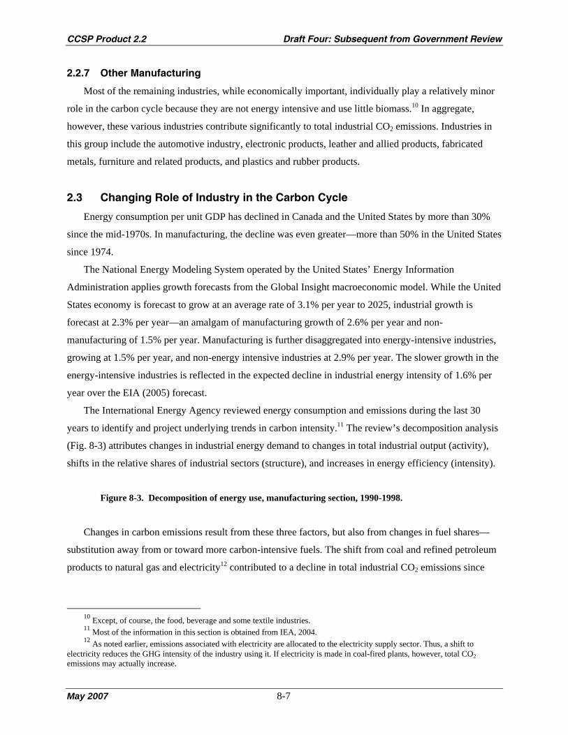
CCSP Product 2.2 Draft Four: Subsequent from Government Review
May 2007 8-7
2.2.7 Other Manufacturing
Most of the remaining industries, while economically important, individually play a relatively minor
role in the carbon cycle because they are not energy intensive and use little biomass.10 In aggregate,
however, these various industries contribute significantly to total industrial CO2 emissions. Industries in
this group include the automotive industry, electronic products, leather and allied products, fabricated
metals, furniture and related products, and plastics and rubber products.
2.3 Changing Role of Industry in the Carbon Cycle
Energy consumption per unit GDP has declined in Canada and the United States by more than 30%
since the mid-1970s. In manufacturing, the decline was even greater—more than 50% in the United States
since 1974.
The National Energy Modeling System operated by the United States’ Energy Information
Administration applies growth forecasts from the Global Insight macroeconomic model. While the United
States economy is forecast to grow at an average rate of 3.1% per year to 2025, industrial growth is
forecast at 2.3% per year—an amalgam of manufacturing growth of 2.6% per year and non-
manufacturing of 1.5% per year. Manufacturing is further disaggregated into energy-intensive industries,
growing at 1.5% per year, and non-energy intensive industries at 2.9% per year. The slower growth in the
energy-intensive industries is reflected in the expected decline in industrial energy intensity of 1.6% per
year over the EIA (2005) forecast.
The International Energy Agency reviewed energy consumption and emissions during the last 30
years to identify and project underlying trends in carbon intensity.11 The review’s decomposition analysis
(Fig. 8-3) attributes changes in industrial energy demand to changes in total industrial output (activity),
shifts in the relative shares of industrial sectors (structure), and increases in energy efficiency (intensity).
Figure 8-3. Decomposition of energy use, manufacturing section, 1990-1998.
Changes in carbon emissions result from these three factors, but also from changes in fuel shares—
substitution away from or toward more carbon-intensive fuels. The shift from coal and refined petroleum
products to natural gas and electricity12 contributed to a decline in total industrial CO2 emissions since
10 Except, of course, the food, beverage and some textile industries. 11 Most of the information in this section is obtained from IEA, 2004. 12 As noted earlier, emissions associated with electricity are allocated to the electricity supply sector. Thus, a shift to
electricity reduces the GHG intensity of the industry using it. If electricity is made in coal-fired plants, however, total CO2 emissions may actually increase.

CCSP Product 2.2 Draft Four: Subsequent from Government Review
May 2007 8-8
1997 in both Canada and the United States. The continuation of this trend is uncertain given the rise in
natural gas prices relative to coal in recent years.
2.4 Actions and Policies for Carbon Management in Industry
Industry managers can reduce carbon flows through industry by altering the material or energy
intensity and character of production (IPCC, 2001). Greater materials efficiency typically reduces energy
demands in processing because of reduced materials handling. For example, recycling materials often
reduces energy consumption per unit of output by 26 to 95% (Table 8-1). Further work on materials
substitution also holds promise for reduced energy consumption and emissions reduction.13
Table 8-1. Energy reductions in recycling.
The prospects for greater energy efficiency are equally substantial. Martin et al. (2001) characterized
more than 50 key emerging energy efficient technologies, including efficient Hall-Heroult cell retrofits,
black liquor gasification in pulp production, and shape casting in steel industries. Worrell et al. (2004)
covers many of the same technologies and notes that significant potential exists in utilizing efficient
motor systems and advanced cogeneration technologies.
At the same time, energy is a valuable production input that, along with capital, can substitute for
labor as a means of increasing productivity. Thus, overall productivity gains in industry can be both
energy-saving and energy-augmenting, and the net impact depends on the nature of technological
innovation and the expected long-run cost of energy relative to other inputs. This suggests that, if policies
to manage carbon emissions from industry were to be effective, they would need to provide a significant
signal to technology innovators and adopters to reflect the negative value that society places on carbon
emissions. This in turn suggests the application of regulations or financial instruments, examples being
energy efficiency regulations, carbon management regulations, and fees on carbon emissions.
3. WASTE MANAGEMENT CARBON CYCLE
The carbon cycle associated with human wastes includes industrial, commercial, construction,
demolition, and residential waste. Municipal solid waste contains significant amounts of carbon. Paper,
plastics, yard trimmings, food scraps, wood, rubber, and textiles made up more than 80% of the 236 Mt of
municipal solid waste generated in the United States in 2003 (EPA, 2005) and the 25 Mt generated in
Canada (Statistics Canada, 2004), as shown in Table 8-2. In Mexico, as much as 20% of wastes are not
systematically collected; no disaggregated data are available (EPA, 2005).
13 For example, substitute petrochemical feedstocks by biomass or concrete by wood in home foundations.
CCSP Product 2.2 Draft Four: Subsequent from Government Review
May 2007 8-9
Table 8-2. Waste materials flows by region in North America, 2003.
A portion of municipal solid waste is recycled: 31% in the United States (EPA 2003b)† and 27% in
Canada (Statistics Canada 2004).† Up to 14% of the remaining waste is incinerated in the United States,
slightly less in Canada. Incineration can reduce the waste stream by up to 80%, but this ensures that more
of the carbon reaches the atmosphere as opposed to being sequestered (or subsequently released as
methane) in a landfill. Incineration, however, can be used to cogenerate electricity and useful heat, which
may reduce carbon emissions from stand-alone facilities.
Once in a landfill, carbon in wastes may be acted upon biologically, releasing roughly equal amounts
of CO2 and methane (CH4) by volume14 depending on ambient conditions, as well as a trace amount of
carbon monoxide and volatile organic compounds. While no direct data on the quantity of CO2 released
from landfills exists, one can estimate the CO2 released by using this ratio; the estimated amount of CO2
released from landfills in Canada and the United States (no data from Mexico) would be approximately
38 Mt,15 a relatively small amount compared to the total of other subsectors in this chapter. Also, recall
that these emissions are from biomass and, in the context of IPCC assessment guidelines, are considered
GHG-neutral.
Depending on the degree to which aerobic or anaerobic metabolism takes place, a considerable
amount of carbon remains unaltered and more or less permanently stored in the landfill (75%-80%; see
Barlaz and Ham, 1990, Barlaz, 1994; and Bogner and Spokas, 1993). Because data on the proportions of
carboniferous material entering landfills can be estimated, approximate carbon contents of these materials
can be determined and the degree to which these materials can decompose, it would be possible to
estimate the amount of carbon sequestered in a landfill site (see EPIC, 2002; Mohareb et al., 2003; EPA,
2003b; EPA, 2005). While EPA (2005) provides an estimate of carbon sequestered in US landfills (see
Table 8-2), no data are available for other regions.
Anaerobic digestion generates methane gases that can be captured and used in cogenerators. Many of
the 1,800 municipal solid waste sites in 2003 in the United States captured and combusted landfill-
generated methane; about half of all the methane produced was combusted or oxidized in some way
(EPA, 2005). In Canada, about 23% of the methane emissions were captured and utilized to make energy
in 2002 (Mohareb et al., 2003). The resultant CO2 released from such combustion is considered biological
in origin. Thus, only methane emissions, at 21 times the CO2 warming potential, are included as part of
GHG inventories. Their combustion greatly alleviates the net contribution to GHG emissions and, if used
14 Based on gas volumes, this means that roughly equivalent amounts of carbon are released as CO2 as CH4. 15 14 Mt of CH4 (see Table 8-3) are equivalent, volume wise at standard temperature and pressure, to 38 Mt of CO2. This
derived estimate is highly uncertain and not of the same caliber as other emissions data provided here.
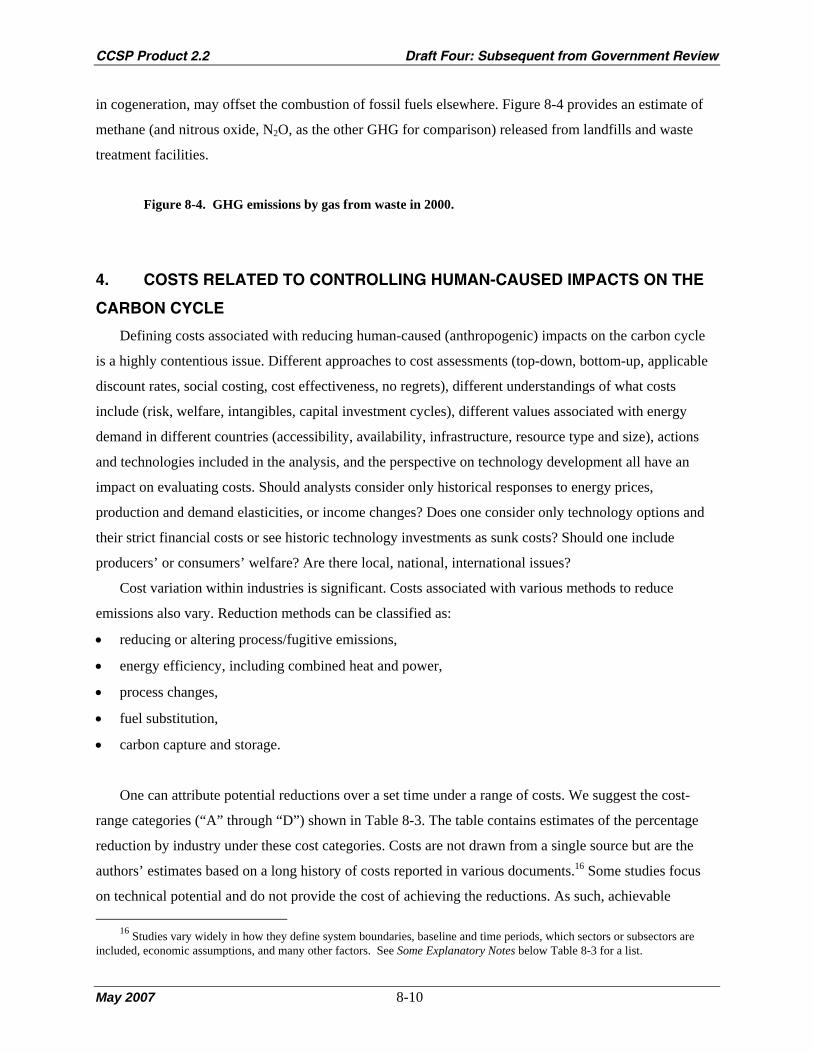
CCSP Product 2.2 Draft Four: Subsequent from Government Review
May 2007 8-10
in cogeneration, may offset the combustion of fossil fuels elsewhere. Figure 8-4 provides an estimate of
methane (and nitrous oxide, N2O, as the other GHG for comparison) released from landfills and waste
treatment facilities.
Figure 8-4. GHG emissions by gas from waste in 2000.
4. COSTS RELATED TO CONTROLLING HUMAN-CAUSED IMPACTS ON THE
CARBON CYCLE
Defining costs associated with reducing human-caused (anthropogenic) impacts on the carbon cycle
is a highly contentious issue. Different approaches to cost assessments (top-down, bottom-up, applicable
discount rates, social costing, cost effectiveness, no regrets), different understandings of what costs
include (risk, welfare, intangibles, capital investment cycles), different values associated with energy
demand in different countries (accessibility, availability, infrastructure, resource type and size), actions
and technologies included in the analysis, and the perspective on technology development all have an
impact on evaluating costs. Should analysts consider only historical responses to energy prices,
production and demand elasticities, or income changes? Does one consider only technology options and
their strict financial costs or see historic technology investments as sunk costs? Should one include
producers’ or consumers’ welfare? Are there local, national, international issues?
Cost variation within industries is significant. Costs associated with various methods to reduce
emissions also vary. Reduction methods can be classified as:
• reducing or altering process/fugitive emissions,
• energy efficiency, including combined heat and power,
• process changes,
• fuel substitution,
• carbon capture and storage.
One can attribute potential reductions over a set time under a range of costs. We suggest the cost-
range categories (“A” through “D”) shown in Table 8-3. The table contains estimates of the percentage
reduction by industry under these cost categories. Costs are not drawn from a single source but are the
authors’ estimates based on a long history of costs reported in various documents.16 Some studies focus
on technical potential and do not provide the cost of achieving the reductions. As such, achievable
16 Studies vary widely in how they define system boundaries, baseline and time periods, which sectors or subsectors are included, economic assumptions, and many other factors. See Some Explanatory Notes below Table 8-3 for a list.

CCSP Product 2.2 Draft Four: Subsequent from Government Review
May 2007 8-11
reductions are likely overestimated. Others describe optimization models that provide normative costs and
likely overestimate potentials and underestimate costs. Still others use top-down approaches where
historic data sets are used to determine relationships between emissions and factors of production; costs
are often high and emissions reductions underestimated.
Table 8-3. Approximate costs and reductions potential.
When looking at cost numbers like this, one should remember that, for each $10 cost increment per t
CO2 (or about $37 per t C), gasoline prices would increase about 2.4¢/L (9¢/U.S. gallon). Diesel fuel cost
would be nearly 2.7¢/L (10¢/U.S. gallon). Costs per Gigajoule (GJ)17 vary by fuel: coal rises about
90¢/GJ, depending on type, HFO by 73¢, and natural gas by 50¢. At 35% efficiency, coal-fired electricity
generation would be about 0.8¢/kWh higher, about 0.65¢/kWh for HFO, and about 0.45¢/kWh for natural
gas.
Of course, as the cost of carbon increases, one moves up the carbon supply curve for industrial
sectors. However, reductions become marginal or insignificant and so are not included in Table 8-3. If a
cell in Table 8-3 shows two cost categories (e.g., A/B) and two reduction levels (%Qred is 15/20), the
value associated with the second portrays the additional reduction at that increased expenditure level.
Thus, spending up to $50/t CO2 to improving efficiency in metal smelting implies a potential reduction of
35% (see Table 8-3). Reductions in each category are not additive for an industry type because categories
are not independent.
Because not all reduction methods are applicable to all industries, as one aggregates to an “all
industry” level (top line, Table 8-3), the total overall emissions reduction level may be less than any of the
individual industries sited.
4.1 Some Explanatory Notes
Data come from a variety of sources and do not delineate costs as per the categories describe here.
Data sources can be notionally categorized into the following groups (with some references listed
twice):18
• General overviews: Grubb et al., 1993; Weyant et al., 1999;19 Grubb et al., 2002; Löschel, 2002.
17 A Gigajoule (GJ), or one billion joules, is slightly smaller than 1 MMBtu (1 GJ = 0.948 MMBtu). 18 Two authors are currently involved with IPCC’s upcoming fourth assessment report where estimated costs of reduction
are provided. Preliminary reviews of the cost data presented there do not differ substantially from those in table 8-3. 19 John Weyant of Stanford University is currently editing another analysis similar to this listed publication to be released in
the near future.

CCSP Product 2.2 Draft Four: Subsequent from Government Review
May 2007 8-12
• Top-down analyses: McKitrick, 1996; Herzog, 1999; Sands, 2002; McFarland et al., 2004; Schäfer
and Jacoby, 2005; Matysek, et al., 2006.
• Bottom up analyses: Martin et al., 2001; Humphreys and Mahasenan, 2002; Worrell et al., 2004; Kim
and Worrell, 2002; Morris et al., 2002; Jaccard et al., 2003a; DOE, 2006; IEA, 2006.
• Hybrid model analyses: Böhringer, 1998; Jacobsen, 1998; Edmonds et al., 2000; Koopmans and te
Velde, 2001; Jaccard, 2002; Frei et al., 2003; Jaccard et al., 2003a; Jaccard et al., 2003b; Edenhofer
et al., 2006.
• Others: Newell et al., 1999; Sutherland, 2000; Jaffe et al., 2002.
4.1.1 Process and Fugitives
Process and fugitive reductions are only available in certain industries. For example, because wood-
products industries burn biomass, fugitives are higher than in other industries and reduction potentials
exist.
In the waste sector, the reductions potentials are very large; we have simply estimated possible
reductions if we were to trap and burn all landfill methane. The costs for this are quite low. EPA (2003a)
estimates of between 40% and 60% of methane available for capture may generate net economic benefits.
4.1.2 Energy Efficiency
The potential for emissions reductions from efficiency improvements is strongly linked with both
process change and fuel switching. For example, moving to Cermet-based processes in electric arc
furnaces in steel and aluminum smelting industries can significantly improve efficiencies and lower both
combustion and process GHG emissions.
A “bottom up” technical analyses tends to show higher potentials and lower costs than when one uses
a hybrid or a “top-down” approach to assess reduction potentials due to efficiency improvements; Table
8-3 portrays the outcome of the more conservative hybrid (mix of top-down and bottom-up) approach and
provides what some may consider conservative estimates of reduction potential (see particularly Martin et
al., 2001; Jaccard et al., 2002; Jaccard et al., 2003a; Jaccard et al., 2003b; Worrell et al., 2004).
4.1.3 Process Change
Reductions from process change requires not only an understanding of the industry and its potential
for change but also an understanding of the market demand for industry products that may change over
time. In pulp production, for example, one could move from higher quality kraft pulp to mechanical pulp
and increase production ratios (the kraft process only converts one-half the input wood into pulp), but will

CCSP Product 2.2 Draft Four: Subsequent from Government Review
May 2007 8-13
market acceptability for the end product be unaffected? Numerous substitution possibilities exist in the
rather diverse Other Manufacturing industries (carpet recycling, alternative uses for plastics, etc.).
4.1.4 Fuel Substitution
It is difficult to isolate fuel substitution and efficiency improvement because fuels display inherent
qualities that affect efficiency. Fuel substitution can reduce carbon flow but efficiency may become
worse. In wood products industries, shifts to biomass reduces emissions but increases energy use. In
terms of higher heating values, shifts from coal or oil to natural gas may worsen efficiencies while
reducing emissions.20
4.1.5 Carbon Capture and Storage (CC&S)
In one sense, all industries and landfills could reduce emissions through CC&S but the range of
appropriate technologies has not been fully defined and/or the costs are very high. For example, one could
combust fuels in a pure oxygen environment such that the exhaust steam is CO2-rich and suitable for
capture and storage. Even so, some industries, like cement production, are reasonable candidates for
capture, but cost of transport of the CO2 to storage may prohibit implementation (see particularly Herzog,
1999; DOE, 2006).
5. RESEARCH AND DEVELOPMENT NEEDS
If we assume that carbon management will play a significant role in the future and that fossil fuels are
likely to remain an economical energy supply for industries, research and development (R&D) will focus
on the control of carbon emissions related to the extraction of this energy. Typical combustion
technologies extract and transform fossil fuels’ chemical energy relatively efficiently but, outside of
further improvements in efficiency, they generally do little to manage the emissions generated. More
recently, advanced technologies remove particularly onerous airborne emissions, such as compounds of
sulphur and nitrogen, particulates, volatile organic compounds and other criteria air contaminants.
However, emissions of carbon dioxide remain relatively unaltered. In the light of changing views on the
impacts of carbon dioxide released to the atmosphere, R&D will likely focus on the extraction of the
energy while preventing carbon dioxide release. Fossil fuels might well remain economically competitive
and socially desirable as a source of energy in some circumstances, even when one includes the extra cost
of capturing the carbon dioxide and preventing its atmospheric release when converting these fuels into
non-carbon secondary forms of energy like electricity, hydrogen or heat.
20 As the ratio of hydrogen to carbon rises in a fossil fuel, more of the total heat released upon combustion is caught up in the latent heat of vaporization of water and is typically lost to process. This loss is equivalent the difference between a fuel’s higher heating value and its lower heating value.

CCSP Product 2.2 Draft Four: Subsequent from Government Review
May 2007 8-14
Some carbon capture and storage processes currently exist; indeed, oil companies have long
“sequestered” carbon dioxide to enhance oil recovery from underground wells simply by injecting it into
the oil reservoir. Many newer processes to accomplish carbon dioxide capture are being investigated,
primarily in two categories: pre-combustion and post-combustion processes. Pre-combustion alternatives
include gasification processes where, for example, coal’s energy is entrapped in hydrogen and the carbon
dioxide stream is subsequently sequestered. Post-combustion alternatives include carbon combustion in
pure oxygen atmospheres and then trapping the resultant carbon dioxide for sequestration, and flue stack
devices designed to extract the carbon dioxide from the flue gases for delivery to sequestration systems.
Research has also been conducted on devices that can extract carbon dioxide directly from the atmosphere
(Keith et al., 2003).
CHAPTER 8 REFERENCES
Barlaz, M.A. and R.K. Ham, 1990: The Use of Mass Balances for Calculation of the Methane Potential of Fresh
and Anaerobically Decomposed Refuse. Proceedings from the GRCDA 13th Annual International Landfill Gas
Symposium, March 27-29, 1990,Silver Spring, MD, GRCDA—The Association of Solid Waste Management
Professionals, 1990, 235 pp.
Barlaz, M., 1994: Measurement of the Methane Potential of the Paper, Yard Waste, and Food Waste Components of
Municipal Solid Waste. Unpublished paper, Department of Civil Engineering, North Carolina State University.
Bogner, J. and K. Spokas, 1993: Landfill CH4: rates, fates, and role in the global carbon cycle. Chemosphere, 26 (1-
4), 369-386.
Böhringer, C., 1998: The synthesis of bottom-up and top-down in energy policy modeling. Energy Economics, 20,
233-48.
California Environmental Protection Agency, 2003: Environmental Technologies and Service Opportunities in
the Baja California Peninsula. International Affairs Unit.
CIEEDAC (Canadian Industrial Energy End-Use Data and Analysis Centre), 2005: Development of Energy
Intensity Indicators for Canadian Industry: 1990-2004. Simon Fraser University, Vancouver, Canada.
DOE, 2006: Accessed on March 27, 2006, U.S. Department of Energy. Available at
www.fossil.energy.gov/programs/sequestration/overview.html
Edenhofer, O., C. Carraro, J. Kohler, and M. Grubb, 2006: The costs of the Kyoto Protocol - a multi-model
evaluation. The Energy Journal, special issue.
Edmonds, J., J. Roop, and M. Scott, 2000: Technology and the Economics of Climate Change Policy. Prepared for
the Pew Center on Climate Change by Battelle National Laboratories.
Energy Information Administration, 2005: International Energy Outlook, 2005.
EPA (Environmental Protection Agency), 2003a: International Analysis of Methane and Nitrous Oxide Abatement
Opportunities: Report to Energy Modeling Forum, Working Group 21.

CCSP Product 2.2 Draft Four: Subsequent from Government Review
May 2007 8-15
EPA (Environmental Protection Agency), 2003b: Municipal Solid Waste in the United States: 2003 Facts and
Figures.
EPA (Environmental Protection Agency), 2005. Inventory of U.S. Greenhouse Gas Emissions and Sinks, 1990-
2003.
EPIC (Environment and Plastics Industry Council), 2002: Opportunities for Reducing Greenhouse Gas Emissions
through Residential Waste Management. Prepared by Environment and Plastics Industry Council.
Grubb, M., J.A. Edmonds, P. ten Brink, and M. Morrison, 1993: The cost of limiting fossil fuel CO2 emissions: a
survey and analysis. Annual Review of Energy and the Environment, 397-478.
Grubb, M., I. Kohler, and D. Anderson, 2002: Induced technical change in energy and environmental modeling:
analytical approaches and policy implications. Annual Review of Energy and the Environment, 27, 271-308.
Frei, C., P. Haldi, and G. Sarlos, 2003: Dynamic formulation of a top-down and bottom-up merging energy policy
model. Energy Policy, 31, 1017-1031.
Hershkowitz, A., 1997: Too Good to Throw Away: Recycling's Proven Record. National Resources Defense
Council. February 1997.
Herzog, H., 1999: The economics of CO2 capture. In: Greenhouse Gas Control Technologies [Reimer P., B.
Eliasson, and A. Wokaum (eds.)]. Elsevier Science Ltd., Oxford, pp. 101-106 (1999).
Humphreys, K. and M. Mahasenan, 2002: Towards A Sustainable Cement Industry - Substudy 8: Climate Change.
World Business Council for Sustainable Development (WBCSD), Geneva, Switzerland.
IEA (International Energy Agency), 2004: 30 Years of Energy Use in IEA Countries.
IEA (International Energy Agency), 2006: Energy Technology Perspectives 2006: Scenarios and Strategies to 2050.
International Energy Agency, Paris, France, 484 pp.
IPCC (Intergovernmental Panel on Climate Change), 2001: Climate Change 2001: Mitigation. Contribution of
Working Group III to the Third Assessment Report of the IPCC, Cambridge University Press, Cambridge, UK.
Jaccard, M., J. Nyboer, and B. Sadownik, 2002: The Cost of Climate Policy. University of British Columbia Press,
Vancouver, British Columbia, Canada.
Jaccard, M., J. Nyboer, C. Bataille, and B. Sadownik, 2003a: Modeling the cost of climate policy: distinguishing
between alternative cost definitions and long-run cost dynamics. The Energy Journal, 24(1), 49-73.
Jaccard, M., R. Loulou, A. Kanudia, J. Nyboer, A. Bailie, and M. Labriet, 2003b: Methodological contrasts in
costing GHG abatement policies: optimization and simulation modeling of micro-economic effects in Canada.
European Journal of Operations Research, 145(1), 148-164.
Jacobsen, H., 1998: Integrating the bottom-up and top-down approach to energy-economy modeling: the case of
Denmark. Energy Economics, 20(4), 443-461.
Jaffe, A., R. Newell, and R. Stavins, 2002: Environmental policy and technological change. Environmental and
Resource Economics, 22, 41-69.
Keith, D.W., and M. Ha-Duong, 2003: CO2 capture from the air: Technology assessment and implications for
climate policy. Proceedings of the 6th Greenhouse Gas Control Conference, Kyoto, Japan [J. Gale and Y. Kaya
(eds.)]. Permagon Press, Oxford, UK, p. 187-197.
CCSP Product 2.2 Draft Four: Subsequent from Government Review
May 2007 8-16
Kim, Y. and E. Worrell, 2002: International comparison of CO2 emissions trends in the iron and steel industry.
Energy Policy, 30, 827-838.
Koopmans, C.C. and D.W. te Velde, 2001: Bridging the energy efficiency gap: using bottom-up information in a
top-down energy demand model. Energy Economics, 23(1), 57-75.
Löschel, A., 2002: Technological change in economic models of environmental policy: a survey. Ecological
Economics, 43, 105-126.
Martin, N., E. Worrell, M. Ruth, L. Price, R.N. Elliott, A.M. Shipley, and J. Thorne, 2001: Emerging Energy-
Efficient Industrial Technologies: New York State Edition. LBNL Report Number 46990, American Council for
an Energy-Efficient Economy (ACEEE).
Matysek, A., M. Ford, G. Jakeman, A. Gurney, K. Low, and B.S. Fisher, 2006: Technology for Development and
Climate. ABARE Research Report 06.6, Canberra, Australia.
McFarland, J., J. Reilly, and H. Herzog, 2004: Representing energy technologies in top-down economic models
using bottom-up information. Energy Economics, 26, 685-707.
McKitrick, R., 1996: The Economic Consequences of Taxing Carbon Emissions in Canada. Department of
Economics, University of British Columbia.
Mohareb, A.K., M. Warith, and R.M. Narbaitz, 2003: Strategies for the municipal solid waste sector to assist
Canada in meeting its Kyoto Protocol commitments. Environmental Review, 12, 71-95.
Morris, S., G. Goldstein, and V. Fthenakis, 2002: NEMS and MARKAL-MACRO models for energy-
environmental-economic analysis: a comparison of the electricity and carbon reduction projections.
Environmental Modeling and Assessment, 17, 207-216.
Newell, R., A. Jaffe, and R. Stavins, 1999: The induced innovation hypothesis and energy-saving technological
change. Quarterly Journal of Economics, 941-975.
Sands, R., 2002: Dynamics of carbon abatement in the second generation model. Energy Economics, 26(4), 721-
738.
Schäfer, A. and H. Jacoby, 2005: Technology detail in a multi-sector CGE model: transport under climate policy.
Energy Economics, 27, 1-24.
Statistics Canada, 2004: Human Activity and the Environment. Statistics Canada, Cat no.16-201-XIE.
Sutherland, R., 2000: “No cost” efforts to reduce carbon emissions in the U.S.: an economic perspective. Energy
Journal, 21(3), 89-112.
Weyant, J., H. Jacoby, J. Edmonds, and R. Richels, 1999: The costs of the Kyoto Protocol - a multi-model
evaluation. The Energy Journal, special issue.
WRI (World Resources Institute), 2005: Climate Analysis Indicators Tool (CAIT), Version 3.0, Washington, DC.
Available at http://cait.wri.org
Worrell, E., L.K. Price, and C. Galitsky, 2004: Emerging Energy-Efficient Technologies in Industry: Case Studies
of Selected Technologies. Environmental Technologies Division, Lawrence Berkeley Laboratory, University of
California at Berkeley.

CCSP Product 2.2 Draft Four: Subsequent from Government Review
May 2007 8-17
Table 8-1. Energy reductions in recycling
Recycled material Energy saved Recycled material Energy saved
Aluminum 95% Glass 31% Tissue paper 54% Newsprint 45% Printing/writing paper 35% Corrugated cardboard 26% Plastics 57%-75% Steel 61%
Source: Hershkowitz, 1997.
Table 8-2. Waste materials flows by region in North America, 2003
United States Canada Mexico
Total waste (Mt yr-1) 236.0 24.8 29.2 Recycled 72.0 6.6 - Carbon-based waste 197.1 19.6 - Carbon-based waste recycled 47.3* 4.3 - Carbon sequestered (CO2 equivalents) 10.1 - - Methane (kt yr-1) Generated 12,486 1,452 - Captured, oxidized 6,239 336 - Emitted 6,247 1,117 - Emitted (CO2 equivalents) 131,187 23,453 -
* Calculated estimate Source: EPA, 2003b, 2005; Statistics Canada, 2004; Mohareb, 2003 for Canada methane data;
California Environmental Protection Agency, 2003 for Mexico data point.
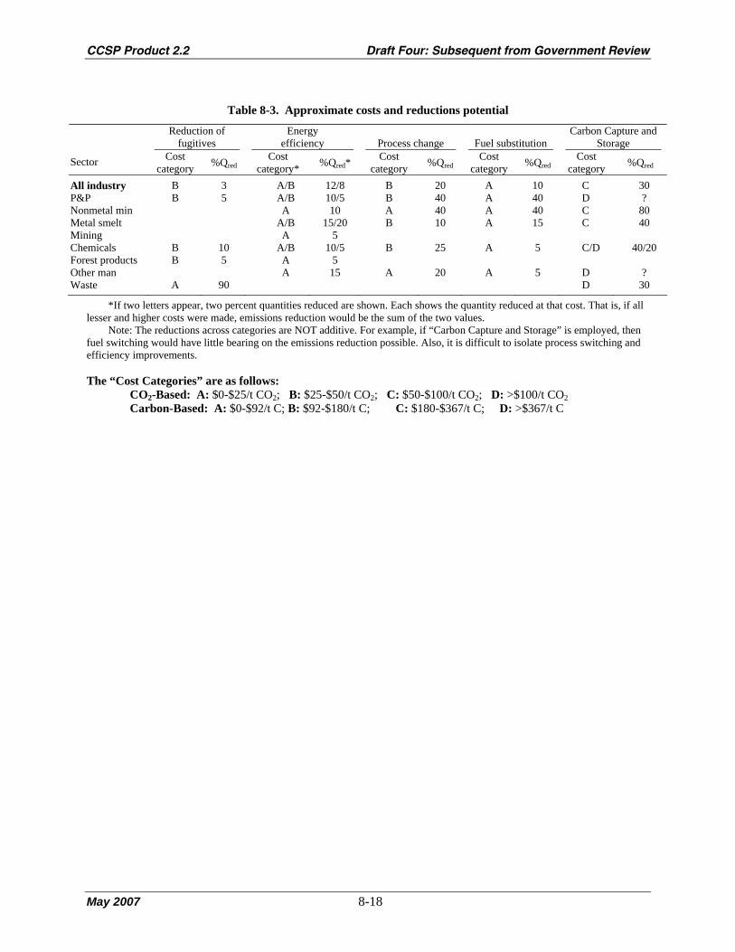
CCSP Product 2.2 Draft Four: Subsequent from Government Review
May 2007 8-18
Table 8-3. Approximate costs and reductions potential
Reduction of fugitives
Energy efficiency
Process change
Fuel substitution
Carbon Capture and Storage
Sector Cost
category %Qred Cost
category* %Qred* Cost category %Qred
Cost category %Qred
Cost category %Qred
All industry B 3 A/B 12/8 B 20 A 10 C 30 P&P B 5 A/B 10/5 B 40 A 40 D ? Nonmetal min A 10 A 40 A 40 C 80 Metal smelt A/B 15/20 B 10 A 15 C 40 Mining A 5 Chemicals B 10 A/B 10/5 B 25 A 5 C/D 40/20 Forest products B 5 A 5 Other man A 15 A 20 A 5 D ? Waste A 90 D 30
*If two letters appear, two percent quantities reduced are shown. Each shows the quantity reduced at that cost. That is, if all lesser and higher costs were made, emissions reduction would be the sum of the two values.
Note: The reductions across categories are NOT additive. For example, if “Carbon Capture and Storage” is employed, then fuel switching would have little bearing on the emissions reduction possible. Also, it is difficult to isolate process switching and efficiency improvements.
The “Cost Categories” are as follows: CO2-Based: A: $0-$25/t CO2; B: $25-$50/t CO2; C: $50-$100/t CO2; D: >$100/t CO2
Carbon-Based: A: $0-$92/t C; B: $92-$180/t C; C: $180-$367/t C; D: >$367/t C
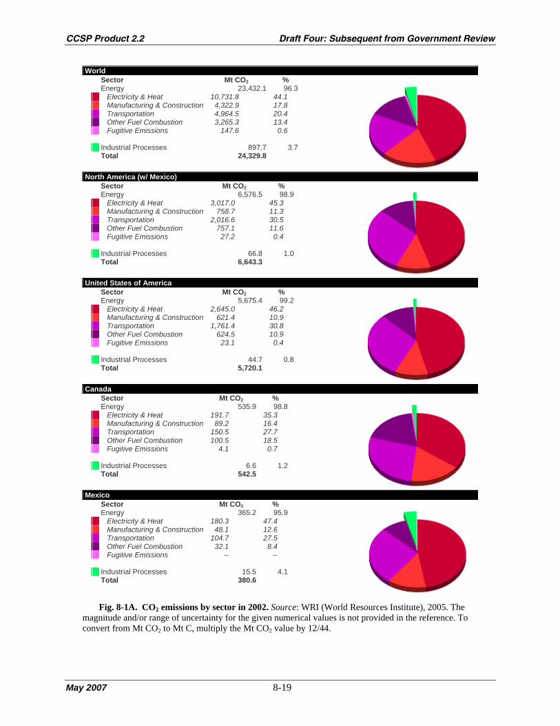
CCSP Product 2.2 Draft Four: Subsequent from Government Review
May 2007 8-19
World Sector Mt CO2 %
Energy 23,432.1 96.3 Electricity & Heat 10,731.8 44.1 Manufacturing & Construction 4,322.9 17.8 Transportation 4,964.5 20.4 Other Fuel Combustion 3,265.3 13.4 Fugitive Emissions 147.6 0.6 Industrial Processes 897.7 3.7 Total 24,329.8
North America (w/ Mexico) Sector Mt CO2 %
Energy 6,576.5 98.9 Electricity & Heat 3,017.0 45.3 Manufacturing & Construction 758.7 11.3 Transportation 2,016.6 30.5 Other Fuel Combustion 757.1 11.6 Fugitive Emissions 27.2 0.4 Industrial Processes 66.8 1.0 Total 6,643.3
United States of America Sector Mt CO2 %
Energy 5,675.4 99.2 Electricity & Heat 2,645.0 46.2 Manufacturing & Construction 621.4 10.9 Transportation 1,761.4 30.8 Other Fuel Combustion 624.5 10.9 Fugitive Emissions 23.1 0.4
Industrial Processes 44.7 0.8 Total 5,720.1
Canada Sector Mt CO2 %
Energy 535.9 98.8 Electricity & Heat 191.7 35.3 Manufacturing & Construction 89.2 16.4 Transportation 150.5 27.7 Other Fuel Combustion 100.5 18.5 Fugitive Emissions 4.1 0.7
Industrial Processes 6.6 1.2 Total 542.5
Mexico Sector Mt CO2 %
Energy 365.2 95.9 Electricity & Heat 180.3 47.4 Manufacturing & Construction 48.1 12.6 Transportation 104.7 27.5 Other Fuel Combustion 32.1 8.4 Fugitive Emissions -- --
Industrial Processes 15.5 4.1 Total 380.6
Fig. 8-1A. CO2 emissions by sector in 2002. Source: WRI (World Resources Institute), 2005. The magnitude and/or range of uncertainty for the given numerical values is not provided in the reference. To convert from Mt CO2 to Mt C, multiply the Mt CO2 value by 12/44.

CCSP Product 2.2 Draft Four: Subsequent from Government Review
May 2007 8-20
World Sector Mt CO2 equiv. %
Energy 24,789.9 74.5 Electricity & Heat 10,269.4 30.9 Manufacturing & Construction 4,327.9 13.0 Transportation 4,809.7 14.5 Other Fuel Combustion 3,742.4 11.2 Fugitive Emissions 1,640.5 4.9
Industrial Processes 1,366.8 4.1 Agriculture 5,631.5 16.9 Waste 1,483.6 4.5 Total 33,271.8
North America (w/ Mexico) Sector Mt CO2 equiv. %
Energy 7,004.8 86.2 Electricity & Heat 3,027.6 37.3 Manufacturing & Construction 809.6 10.0 Transportation 1,971.1 24.3 Other Fuel Combustion 877.2 10.8 Fugitive Emissions 319.2 3.9 Industrial Processes 239.0 2.9 Agriculture 580.9 7.1 Waste 300.0 3.7 Total 8,124.7
United States of America Sector Mt CO2 equiv. %
Energy 6,005.5 86.8 Electricity & Heat 2,670.6 38.6 Manufacturing & Construction 657.9 9.5 Transportation 1,719.9 24.9 Other Fuel Combustion 723.6 10.5 Fugitive Emissions 233.5 3.4 Industrial Processes 198.4 2.9 Agriculture 469.9 6.8 Waste 243.3 3.5 Total 6,917.1
Canada Sector Mt CO2 equiv. %
Energy 589.5 85.0 Electricity & Heat 185.9 26.8 Manufacturing & Construction 94.6 13.6 Transportation 150.0 21.6 Other Fuel Combustion 115.3 16.6 Fugitive Emissions [1] 43.6 6.3 Industrial Processes [2] 19.3 2.8 Agriculture 60.8 8.8 Waste 24.2 3.5 Total 693.8
Mexico Sector Mt CO2 equiv. %
Energy 409.8 79.8 Electricity & Heat 171.1 33.3 Manufacturing & Construction 57.1 11.1 Transportation 101.2 19.7 Other Fuel Combustion 38.3 7.5 Fugitive Emissions [1] 42.1 8.2 Industrial Processes [2] 21.3 4.2 Agriculture 50.2 9.8 Waste 32.5 6.3 Total 513.8
[1] N2O data not available. [2] CH4 data not available. 1
Fig. 8-1B. GHG emissions by sector in 2000, CO2, CH4, N2O, PFCs, HFCs, and SF6. Source: WRI (World Resources 2 Institute), 2005. The magnitude and/or range of uncertainty for the given numerical values is not provided in the reference. 3
To convert from Mt CO2 equivalent to Mt C equivalent, multiply the Mt CO2 value by 12/44. 4

CCSP Product 2.2 Draft Four: Subsequent from Government Review
May 2007 8-21
1
Fig. 8-2. Carbon flows for Canada, the United States and Mexico combined. Values in megatons carbon
can be converted to megatons CO2 equivalents by multiplying by 44/12, the ratio of carbon dioxide mass to carbon mass. Comparable diagrams for the individual countries are in Appendix 8A. Source: Energy data from Statistics Canada Industrial Consumption of Energy survey, Conversion coefficients, IEA Oil Information 2004, IEA Coal Information 2005, IEA Natural Gas Information 2004. Process emissions from Environment Canada, Canada GHG Inventory, 2002, EPA, U.S. Emissions Inventory. Production data from Statistics Canada, CANSIM Table 002-0010, Tables 303-0010, -0014 to -0021, -0024, -0060, Pub. Cat. Nos.: 21-020, 26-002, 45-002, Canadian Pulp and Paper Association on forestry products. Production of forestry products: USDA Database; FO-2471000, -2472010, -2482000, -2483040, -6342000, -6342040, U.S. Timber Production, Trade, Consumption, and Price Statistics 1965-2005. Production of organic products (e.g., food): USDA PS&D Official Statistical Results. Steel: International Iron and Steel institute, World steel in figures 2003. Minerals production: USGS mineral publications.

CCSP Product 2.2 Draft Four: Subsequent from Government Review
May 2007 8-22
1
Fig. 8-3. Decomposition of energy use, manufacturing sector, 1990-1998. Source: IEA, 2004.

CCSP Product 2.2 Draft Four: Subsequent from Government Review
May 2007 8-23
World
Gas Mt CO2
equivalent %
CH4 1,386.4 93.5 N2O 97.2 6.5 Total 1,483.6
North America (w/ Mexico)
Gas Mt CO2
equivalent %
CH4 281.8 93.9 N2O 18.2 6.1 Total 300.0
United States of America
Gas Mt CO2
equivalent %
CH4 227.7 93.6 N2O 15.6 6.4 Total 243.3
Canada
Gas Mt CO2
equivalent %
CH4 23.2 95.8 N2O 1.0 4.2 Total 24.2
Mexico
Gas
Mt CO2 equivalent %
CH4 31.0 95.2 N2O 1.6 4.8 Total 32.5
1
Fig. 8-4. GHG emissions by gas from waste in 2000. Source: WRI (World Resources Institute), 2005. The 2 magnitude and/or range of uncertainty for the given numerical values is not provided in the reference. 3
To convert from Mt CO2 equivalent to Mt C equivalent, multiply the Mt CO2 value by 12/44. 4

CCSP Product 2.2 Draft Four: Subsequent from Government Review
May 2007 8-24
[This page intentionally left blank] 1

CCSP Product 2.2 Draft Four: Subsequent from Government Review
May 2007 9-1
Chapter 9. Buildings
Lead Author: James E. McMahon1
Contributing Authors: Michael A. McNeil1, Itha Sánchez Ramos2
1Lawrence Berkeley National Laboratory, 2Instituto de Investigaciones Eléctricas, Cuernavaca, Mexico
KEY FINDINGS
• The buildings sector of North America was responsible for annual carbon dioxide emissions of 671
million tons of carbon in 2003, which is 37% of total North American carbon dioxide emissions and
10% of global emissions. United States buildings alone are responsible for more carbon dioxide
emissions than total carbon dioxide emissions of any other country in the world, except China.
• Carbon dioxide emissions from energy use in buildings in the United States and Canada increased by
30% from 1990 to 2003, an annual growth rate of 2.1% per year.
• Carbon dioxide emissions from buildings have grown with energy consumption, which in turn is
increasing with population and income. Rising incomes have led to larger residential buildings and
increased household appliance ownership.
• These trends are likely to continue in the future, with increased energy efficiency of building materials
and equipment and slowing population growth, especially in Mexico, only partially offsetting the
general growth in population and income.
• Options for reducing the carbon dioxide emissions of new and existing buildings include increasing
the efficiency of equipment and implementing insulation and passive design measures to provide
thermal comfort and lighting with reduced energy. Current best practices can reduce emissions from
buildings by at least 60% for offices and 70% for homes. Technology options could be supported by a
portfolio of policy options that take advantage of cooperative activities, avoid unduly burdening certain
sectors, and are cost effective.
• Because reducing carbon dioxide emissions from buildings is currently secondary to reducing building
costs, continued improvement of energy efficiency in buildings and reduced carbon dioxide emissions
from the building sector will require a better understanding of the total societal cost of carbon dioxide
emissions as an externality of building costs, including the costs of mitigation compared to the costs
of continued emissions.

CCSP Product 2.2 Draft Four: Subsequent from Government Review
May 2007 9-2
1. BACKGROUND In 2003, buildings were responsible for 615 million tons of carbon (Mt C)1
emitted in the United
States (DOE/EIA, 2005), 40 Mt C in Canada (Natural Resources Canada, 2005) and 17 Mt C in Mexico
(SENER México, 2005), for a total of 671 Mt C in North America.† According to the International Energy
Agency, total energy-related emissions in North America in this year were 1815 Mt C (IEA, 2005).
Therefore, buildings were responsible for 37% of energy-related emissions in North America. North
American buildings accounted for 10% of global energy emissions, which totaled 6814 Mt C. United
States buildings alone are responsible for more carbon dioxide (CO2) emissions than total CO2 emissions
of any other country in the world except China (Kinsey et al., 2002). Significant carbon emissions are due
to energy consumption during the operation of the buildings; other emissions, not well quantified, may
occur from water use in and around the buildings and from land-use impacts related to buildings.
Buildings are responsible for 72% of United States electricity consumption and 54% of natural gas
consumption (DOE/EERE, 2005).2 The discussions in this chapter include an accounting of CO2
emissions from electricity consumed in the buildings sector; however, this represents a potential double
counting of the CO2 emissions from fossil fuels that are used to generate that electricity (see Chapter 6).
This chapter provides a description of how energy, including electrical energy, is used within the
buildings sector. Following the discussion of such end uses of energy, this chapter then describes the
opportunities and potential for reducing energy consumption within the sector.
Many options are available for reducing the carbon impacts of new and existing buildings, including
increasing equipment efficiency and implementing alternative design, construction, and operational
measures to provide thermal comfort and lighting with reduced energy. Current best practices can reduce
carbon emissions for buildings by at least 60% for offices3 and up to 70% for homes.4 Residential and
commercial buildings in the United States and Canada occupy 27 billion m2 (2.7 million hectares)† of
floor space, providing a large area available for siting non-carbon-emitting on-site energy supplies (e.g.,
photovoltaic panels on roofs)5. With the most cutting-edge technology, at the least, emissions can be
dramatically reduced, and, at best, buildings can produce electricity without carbon emissions by means
of on-site renewable electricity generation.
1 Carbon dioxide emissions only. † The magnitude and/or range of uncertainty for the given numerical value(s) is not provided in the references cited. 2 See Tables 1.1.6 and 1.1.7 in DOE/EERE (2005). 3 Leadership in Energy and Environment Design (LEED) Gold Certification (USGBC, 2005). 4 U.S. DOE Building America Program (DOE/EERE, 2006). 5 A recent study estimates a potential of 711 GW generation capacity from rooftop installation of photovoltaic systems (Chaudhari et al., 2004).

CCSP Product 2.2 Draft Four: Subsequent from Government Review
May 2007 9-3
2. CARBON FLUXES
Carbon fluxes from energy emissions in buildings are well understood, since primary energy inputs
from the source of production are tracked, their emissions rates are known, and the total end user
consumption data are gathered and reported by energy utilities, typically monthly. The quantity of energy
consumed by each particular end use is slightly less well known because attribution requires detailed data
on use patterns in a wide variety of contexts. The governments of North America have invested in
detailed energy consumption surveys, which allow researchers to identify opportunities for reducing
energy use.
The largest contribution to carbon emissions from buildings is through the operation of energy-using
equipment. The energy consumed in the average home accounts for 2.9 metric tons6 of carbon per year in
the United States, 1.7 metric tons7 per year in Canada, and 0.6 metric tons8 in Mexico (DOE/EIA, 2005;
Natural Resources Canada, 2005; SENER México, 2004).† Energy consumption in a 500-m2 commercial,
government, or public-use building in the United States produces 1.9 metric tons of carbon (DOE/EIA,
2005).9† Energy consumption includes electricity as well as the direct combustion of fossil fuels (natural
gas, bottled gas and petroleum distillates) and the burning of wood. Because most electricity in North
America is produced from fossil fuels, each kilowatt-hour consumed in a building contributed about 180 g
of carbon to the atmosphere in 2003 (DOE/EIA, 2005).10 The equivalent amount of energy from natural
gas or other fuels contributed about 52 g of carbon (DOE/EIA, 2005).11 Renewable energy accounted for
9% of electricity production in 2003, down from 12% in 1990. Renewable site energy use in buildings
also decreased in that time, from 4% to 2%, mostly due to decreasing use of wood as a household fuel
(DOE/EERE, 2005).12
Buildings-sector CO2 emissions and the relative contribution of each end use are shown in Fig. 9-1. In
the United States, five end uses account for 87% of primary energy consumption in buildings: space
conditioning (including space heating, cooling and ventilation), 40.9%; lighting, 19.8%; water heating,
10.5%; refrigeration, 7.9%; and electronics (including televisions, computers, and office equipment),
7.7% (DOE/EERE, 2005).13† Space heating and cooling are the largest single uses for residences,
commercial, and public-sector buildings, accounting for 46% and 35% of primary energy, respectively, in
6 U.S. residential sector emissions of 334 Mt CO2 divided by 114 million households in 2004; the numerical value given for “tons of carbon” is for carbon dioxide emissions only. 7 Canada residential sector emissions of 20.6 Mt CO2 divided by 12.2 million households in 2003. 8 Mexico residential sector emissions of 13.2 Mt CO2 divided by 23.8 million households in 2004. 9 U.S. commercial sector emissions per m2 in 2003 times 500 m2. 10 U.S. emissions from electricity divided by delivered energy. 11 U.S. emissions from electricity divided by delivered energy. 12 See Table 1.1.2 and Summary Table 2 in DOE/EERE (2005). 13 Does not include adjustment EIA uses to relieve differences between data sources.

CCSP Product 2.2 Draft Four: Subsequent from Government Review
May 2007 9-4
the United States (DOE/EERE, 2005).14 Water heating is the second-highest energy consumer in the
United States and Canada, while lighting is the second-highest source of CO2 emissions, due to the higher
emissions per unit of electricity compared to natural gas.
Fig. 9-1. U.S. carbon emissions by sector and—for commercial and residential buildings—by end
use.
Heating and cooling loads are highly climate dependent; colder regions use heating during much of
the year (primarily with natural gas), while warm regions seldom use heating. The majority of United
States households own an air conditioner; and, although air-conditioner ownership has been historically
low in Mexico,15 sales of this equipment are now growing significantly, 14% per year over the past 10
years.16 Space-conditioning energy end use depends significantly on building construction (e.g.,
insulation, air infiltration) and operation (thermostat settings). Water heating is a major consumer of
energy in the United States and Canada, where storage-tank systems are common.
Aside from heating and cooling, lighting, and water heating, energy is consumed by a variety of
appliances, mostly electrical. Most homes in the United States and Canada own all of the major
appliances, including refrigerators, freezers, clothes washers, clothes dryers, dishwashers, and at least one
color television. The remainder of household energy consumption comes from small appliances (blenders
and microwaves, for example) and increasingly from electronic devices, such as entertainment equipment
and personal computers. In Mexico, 96.6% of households used electricity in 2005, and recent years have
shown a marked growth in appliance ownership: ownership rates in 2000 were 85.9% for televisions,
68.5% for refrigerators, 52% for washing machines, and only 9.3% for computers. By the end of 2005
ownership rates had grown to 91% for televisions, 79% for refrigerators, 62.7% for washing machines,
and 19.6% for computers (INEGI, 2005).
Many end uses—such as water heating, and space heating, cooling, and ventilation—occur in most
commercial sector buildings. Factors such as climate and building construction influence the carbon
emissions by these buildings. In addition, commercial buildings contain specialized equipment, such as
large-scale refrigeration units in supermarkets; cooking equipment in food preparation businesses; and
computers, printers, and copiers in office buildings. Office equipment is the largest component of
electricity use aside from cooling and lighting. Due to heat from internal loads, many commercial
buildings use air-conditioning year round in most climates in North America.
14 Table 1.2.3 and Table 1.3.3 in DOE/EERE (2005); available at http://buildingsdatabook.eere.energy.gov (2003 data). 15 Air conditioners have typically been used only in the northern and coastal areas of Mexico. 16 Air conditioner sales 1995–2004 from Asociacion Nacional de Fabricantes de Aparatos Domesticos (ANFAD).

CCSP Product 2.2 Draft Four: Subsequent from Government Review
May 2007 9-5
Residential and commercial buildings in the United States are responsible for 38% of CO2 emissions
from energy nationally and 33% of emissions from energy in North America as a whole. Total emissions
from buildings in the United States are ten times as high as in the other two countries combined, due to a
large population compared to Canada, and high per capita consumption compared to Mexico. On a per
capita basis, building energy consumption in the United States (65 Gigajoules [GJ] per person per year) is
comparable with that of Canada (75 GJ per person per year).† This is about seven to eight times higher
than in Mexico, where 9 GJ is consumed per person per year.17†
In general, contributions from the residential sector are roughly equal to that of the commercial
sector, except in Mexico, where the commercial sector contributes less. Electricity contributes twice as
many emissions as all other fuels combined in the United States and Mexico (2.2 and 2.1 times as much,
respectively). In Canada, natural gas is on par with electricity (1.03 times as many emissions), due to high
heating loads resulting from the cold climate. Fuel oil represents most of Canada’s “other fuels” for the
commercial sector. Firewood (leña) remains an important fuel for many Mexican households for heating,
water heating, and cooking. Table 9-1 summarizes CO2 emissions by country, sector, and fuel type.
Table 9-1. Carbon dioxide emissions from energy consumed in buildings.
The energy consumed during building operation is the most important input to the carbon cycle from
buildings; but it is not the only one. The construction, renovation, and demolition of buildings also
generate a significant flux of wood and other materials. Construction of a typical 204-m2 (2200-ft2) house
requires about 20 metric tons of wood and creates 2 to 7 metric tons of construction waste (DOE/EERE,
2005).18† Building lifetimes are many decades and, especially for commercial buildings, may include
several cycles of remodeling and renovation. In the United States as a whole, water supplied to residential
and commercial customers accounts for about 6% of total national fresh water consumption. This water
consumption also impacts the carbon cycle because water supply, treatment, and waste disposal require
energy.
3. TRENDS AND DRIVERS
Several factors influence trends in carbon emissions in the buildings sector. Some driver variables
tend to increase emissions, while others decrease emissions. Emissions from energy use in buildings in
17 Total building energy (Source: IEA) divided by population (Source: UN Department of Economic and Social Affairs) United States, 18296 million GJ divided 282 million; Canada 2280 million GJ divided by 30.5 million; Mexico 855 million GJ divided by 97.4 million. 18 Construction data from Table 2.1.7 in DOE/EERE (2005); wood content estimated from lumber content. Construction waste from Table 3.4.1 in DOE/EERE (2005).

CCSP Product 2.2 Draft Four: Subsequent from Government Review
May 2007 9-6
the United States and Canada increased 30% from 1990 to 2003 (DOE/EERE, 2005; Natural Resources
Canada, 2005),19 corresponding to an annual growth rate of 2.1%.
Carbon emissions from buildings have grown with energy consumption, which in turn is increasing
with population and income. Demographic shifts therefore have a direct influence on residential energy
consumption. Rising incomes have led to larger residential buildings—the amount of living area per
capita is increasing in all three countries in North America. On one hand, total population growth is
slowing, especially in Mexico, as families are having fewer children than in the past. Annual population
growth during the 1990s was 1.1% in the United States, 1.0% in Canada, and 1.7% in Mexico. In the
period from 1970 to 1990, it was 1.0%, 1.2%, and 2.5%, respectively.20† By 2005, annual population
growth in Mexico declined to 1% (INEGI, 2005). On the other hand, a shift from large, extended-family
households to nuclear-family and single-occupant households means an increase in the number of
households per unit population21—each with its own heating and cooling systems and appliances.
The consumption of energy on a per capita basis or per unit economic activity [gross domestic
product (GDP)] is also not constant but depends on several underlying factors. Economic development is
a primary driver of overall per capita energy consumption and influences the mix of fuels used.22 Per
capita energy consumption generally grows with economic development, since wealthier people live in
larger dwellings and use more energy.23 Recently, computers, printers, and other office equipment have
become commonplace in nearly all businesses and in most homes. These end uses now constitute 7% of
primary household energy consumption. Because of these growing electricity uses, the ratio of electricity
to total household primary energy has increased. This is significant to emissions because of the large
emissions associated with the combustion of fossil fuels in power plants. Electricity can be generated
from renewable sources, such as solar or wind, but their full potential has yet to be realized.
In the United Stages, the major drivers of energy consumption growth are growth in commercial floor
space and an increase in the size of the average home. The size of an average United States single-family
home has grown from 160 m2 (1720 ft2) for a house built in 1980 to 216 m2 (2330 ft2) in 2003.† In the
same time, commercial floor space per capita has increased from 20 to 22.6 m2 (215 to 240 ft2)
(DOE/EERE, 2005).24† Certain end uses once considered luxuries have now become commonplace. Only
56% of United States homes in 1978 used mechanical space-cooling equipment (DOE/EIA, 2005). By
2001, ownership grew to 83%, driven by near total saturation in warmer climates and a demographic shift
in new construction to these regions. Table 9-2 shows emissions trends, as well as the underlying drivers. 19 Data from Table 3.1.1 in DOE/EERE (2005). 20 Source: UN Department of Economic and Social Affairs. 21 See household size statistics in Table 9-2. 22 For example, whether biomass, natural gas or electricity is used for space heating and cooking. 23 See Table 4.2.6 in DOE/EERE (2005). 24 See Tables 2.1.6 and 2.2.1 in DOE/EERE (2005). Residential data are from 1981.
CCSP Product 2.2 Draft Four: Subsequent from Government Review
May 2007 9-7
Table 9-2. Principal drivers of buildings emissions trends.
[SIDEBAR 1 TEXT BOX HERE]
Although the general trend has been toward growth in per capita emissions, emissions per unit of
GDP have decreased in past decades, due to improvements in efficiency. Efficiency performance of most
types of equipment has generally increased, as has the thermal insulation of buildings, due to influences
such as technology improvements and voluntary and mandatory efficiency standards and building codes.
The energy crisis of the 1970s was followed with a sharp decline in economic energy intensity. Increases
in efficiency were driven both by market-related technology improvements and incentives and by the
establishment of federal and state/provincial government policies designed to encourage or require energy
efficiency.
4. OPTIONS FOR MANAGEMENT
A variety of alternatives exists for reducing emissions from the buildings sector. Technology- and market-driven
improvements in efficiency are expected to continue for most equipment, but this will probably not be sufficient to
curtail emissions growth adequately without government intervention. The government has many different ways in
which it can manage emissions that have been proven effective in influencing the flow of products from
manufacturers to users (Interlaboratory Working Group, 2000). That flow may involve six steps: advancing
technologies; product development and manufacturing; supply, distribution, and wholesale purchasing; retail
purchasing; system design and installation; and operation and maintenance (Wiel and McMahon, 2005). Options for
specific products or packages include government investment in research and development, information and
education programs, energy pricing and metering, incentives and financing, establishment of voluntary guidelines,
procurement programs, energy audits and retrofits, and mandatory regulation. The most effective approaches will
likely include more than one of these options in a policy portfolio that takes advantage of synergies, avoids unduly
burdening certain sectors, and is cost effective. Major participants include not only federal agencies, but also state
and local governments, energy and water utilities, private research and development firms, equipment manufacturers
and importers, energy services companies (ESCOs), nonprofit organizations, building owners and occupants. An
ESCO is a company that offers to reduce a client’s utility costs, often with the cost savings being split
with the client through an energy performance contract or a shared savings agreement.
• Technology adoption supported by research and development: Government has the opportunity
to encourage development and adoption of energy-efficient technologies through investment in
research and development, which can advance technologies and bring down prices, therefore enabling

CCSP Product 2.2 Draft Four: Subsequent from Government Review
May 2007 9-8
a larger market. Successful programs have contributed to the development of high-efficiency lighting,
heating, cooling, and refrigeration. Research and development has also had an impact on the
improvement of insulation, ducting, and windows. Finally, government support of research and
development has been critical in the reduction of costs associated with development of renewable
energy.
• Voluntary Programs: By now, there are a wide range of efficiency technologies and best practices
available, and if the most cost-effective among them were widely utilized, carbon emissions would be
reduced. Voluntary measures can be effective in overcoming some market barriers. Government has
been active with programs to educate consumers with endorsement labels or ratings [such as the U.S.
Environmental Protection Agency’s (EPA’s) and U.S. Department of Energy’s (DOE’s) Energy Star
Appliances and Homes], public-private partnerships [such as DOE’s “Building America Program”].
Government is not the only player, however. Energy utilities can offer rebates for efficient appliances,
and ESCOs can facilitate best practices at the firm level. Finally, nongovernment organizations and
professional societies (such as the U.S. Green Building Council and the American Institute of
Architects) can play a role in establishing benchmarks and ratings.
• Regulations: Governments can dramatically impact energy consumption through well-considered
regulations that address market failures with cost-effective measures. Regulations facilitate best
practices in two ways: they eliminate the lowest-performing equipment from the market, and they
boost the market share of high-efficiency technologies. Widely used examples are mandatory energy
efficiency standards for appliances, equipment, and lighting; mandatory labeling programs; and
building codes. Most equipment standards are instituted at a national level, whereas most states have
their own set of prescriptive building codes (and sometimes energy performance standards for
equipment) to guarantee a minimum standard for energy-saving design in homes and businesses.
[SIDEBAR 2 TEXT BOX HERE]
Although large strides in efficiency improvement have been made over the past three decades,
significant improvements are still possible. They will involve continued improvement in equipment
technology, and will increasingly take a whole-building approach that integrates the design of the
building and the energy consumption of the equipment inside it. The improvements may also involve
alternative ways to provide energy services, such as cogeneration of heat and electricity and thermal
energy storage units (Public Technology Inc. and U.S. Green Building Council, 1996).
Whole-building certification standards evaluate a package of efficiency and design options. An
example is the Leadership in Energy and Environmental Design (LEED) certification system developed
CCSP Product 2.2 Draft Four: Subsequent from Government Review
May 2007 9-9
by the U.S. Green Building Council, a non-profit organization. In existence for five years, the LEED
program has certified 36 million m2 (390 million ft2) of commercial and public-sector buildings and has
recently implemented a certification system for homes. The LEED program includes a graduated rating
system (Certified, Silver, Gold, or Platinum) for environmentally friendly design, of which energy
efficiency is a key component (USGBC, 2005).
On the government side, the EPA’s Energy Star Homes program awards certification to new homes
that are independently verified to be at least 30% more energy-efficient than homes built to the 1993
national Model Energy Code, or 15% more efficient than state energy code, whichever is more rigorous.
Likewise, the DOE’s Building America program partners with homebuilders, providing research and
development toward goals to decrease primary energy consumption by 30% for participating projects by
2007, and by 50% by 2015.
5. RESEARCH AND DEVELOPMENT NEEDS
Research, development, demonstration, and deployment of technologies and programs to improve
energy efficiency in buildings and to produce energy with fewer carbon emissions have involved
significant effort over the last 30 years. These efforts have contributed options toward carbon
management. Technologies and markets continue to evolve, representing new crops of “low-hanging
fruit” available for harvesting. However, in most buildings-related decisions in North America, reducing
carbon emissions remains a secondary objective to other goals, such as reducing first costs (DeCanio,
1993 and 1994). The questions for which answers could significantly change the discussion about options
for carbon management include the following.
• What is the total societal cost of environmental externalities25, including carbon emissions? Energy
resources in North America have been abundant and affordable, but externality costs have not been
completely accounted for. Most economic decisions are weighted toward the short term and do not
consider the complete costs. Total societal costs of carbon emissions are unknown and, because it is a
global issue, difficult to allocate. Practical difficulties notwithstanding, this is a key issue, answers to
which could influence priorities for research and development as well as policies such as energy
pricing, carbon taxes or credits.
• What cost-effective reduced-carbon-emitting equipment and building systems—including energy
demand (efficient equipment) and supply (renewable energy)—are available in the short, medium,
and long term? Policymakers must have sufficient information to be confident that particular new
25 External costs are the costs borne by society beyond those included in the market prices of goods. For example, carbon emissions may cause environmental damage not reflected in the market transactions associated with the buying and selling of energy (Rabl and Spadaro, 2007).

CCSP Product 2.2 Draft Four: Subsequent from Government Review
May 2007 9-10
technology types or programs will be effective and affordable. For consumers to consider a set of
options seriously, the technologies must be manifested as products that are widely available and
competitive in the marketplace. Therefore, economic and market analyses are necessary before
attractive options for managing carbon can be proposed.
• How do the costs of mitigation compare to the costs of continued emissions? The answers to the
previous two questions can be compared in order to develop a supply curve of conserved carbon
comprising a series of least-cost options, whether changes to energy demand or to supply, for
managing carbon emissions. The supply curve of conserved carbon will need to be updated at regular
intervals to account for changes in technologies, production practices, and market acceptance of
competing solutions.
CHAPTER 9 REFERENCES
CEC (California Energy Commission), 2005: California's Water Energy Relationship. Staff Final Report, California
Energy Commission, Sacramento, CA.
Chaudhari, M. et al., 2004: PV Grid Gonnected Market Potential under a Cost Breakthrough Scenario. 1174373,
Navigant Consulting Inc.
CONAFOVI (Comisión Nacional de Fomento a la Vivienda), 2001: Programa Sectoral de Vivienda 2001-2006.
DeCanio, S., 1993: Barriers within firms to energy-efficient investments. Energy Policy, 906-914.
DeCanio, S., 1994: Why do profitable energy-saving investiment projects languish? Journal of General
Management, 20(1), 62-71.
DOE/EERE (U.S. Department of Energy, Energy Efficiency and Renewable Energy), 2005: 2005 Buildings Energy
Data Book. Office of Energy Efficiency and Renewable Energy, Washington, DC.
DOE/EERE (U.S. Department of Energy, Energy Efficiency and Renewable Energy), 2006: Building America Puts
Residential Building Research to Work. Washington, DC. Available at
http://www.eere.energy.gov/buildings/building_america/
DOE/EIA (U.S. Departmenet of Energy and Energy Information Administration), 2003: Carbon Coefficients Used
in Emissions of Greenhouse Gases in the United States. Washington, DC. Available at
http://www.eia.doe.gov/oiaf/1605/ggrpt/pdf/tab6.1.pdf
DOE/EIA (U.S. Department of Energy and Energy Information Administration), 2005: Annual Energy Outlook
2005. Energy Information Administration, EIA-0383(2005), Washington, DC.
IEA (International Energy Agency), 2005: Carbon Dioxide Emissions from Fossil Fuel Combustion,.
INEGI (Instituto Nacional de Estadística Geografía e Informática), 2005: Censo general de población y vivienda
2005. Mexico, D.F., 2005.
Interlaboratory Working Group, 2000: Scenarios for a Clean Energy Future. Prepared by Lawrence Berkeley
National Laboratory (LBNL-44029) and Oak Ridge National Laboratory (ORNL/CON-476) for the U.S.
Department of Energy.
CCSP Product 2.2 Draft Four: Subsequent from Government Review
May 2007 9-11
Kinsey, B.R., et al., 2002: The Federal Buildings Research and Development Program: A Sharp Tool for Climate
Policy. ACEEE Buildings Summer Study 2002, Pacific Grove.
Natural Resources Canada, 2005: Office of Energy Efficiency National Energy Use Database 2005. Ottawa,
Canada. Available at http://oee.nrcan.gc.ca/corporate/statistics/neud/dpa/data_e/database_e.cfm
NRCanada, 2005: Residential Sector Secondary Energy Use and GHG Emissions by End Use 2005. Ottawa,
Canada.
Public Technology Inc. and U.S. Green Building Council, 1996: Sustainable Building Technical Manual.
Rabl, A., and J.V. Spadaro, 2007: "Environmental Impacts and Costs of Energy," Chapter 4 in Handbook of Energy
Efficiency and Renewable Energy, F. Krieth and Y. Goswami (editors), CRC Press, New York, NY.
SENER México, 2004: Balance Nacional de Energía 2003. Subsecretaría de Paneación Energética y Desarrollo
Tecnológico. México D.F.
SENER México, 2005: Secretaria de Energia—Sistema de Información Energética. México D.F. Available at
http://sie.energia.gob.mx/sie/bdiController
USGBC (U.S. Green Building Council), 2005: LEED for New Construction—Rating System 2.2. U.S. Green
Building Council, LEED (NC) 2.2, Washington, DC.
Wiel, S. and J.E. McMahon, 2005: Energy-Efficiency Labels and Standards: A Guidebook for Appliances,
Equipment, and Lighting, 2nd Edition. Collaborative Labeling and Standards Program, Washington, DC.

CCSP Product 2.2 Draft Four: Subsequent from Government Review
May 2007 9-12
[BEGIN SIDEBAR 1 TEXT BOX]
Electricity Consumption in the United States and in California
Since the mid-1970s, the state of California has pursued an aggressive set of efficiency regulations and
utility programs. As a result, per capita electricity consumption has stabilized in that state, while it
continues to grow in the United States as a whole.
Source: California Energy Commission— Available at http://www.energy.ca.gov/2005publications/CEC-999-2005-007/CEC-999-2005-007.PDF, Slide 5
[END SIDEDBAR 1 TEXT BOX]

CCSP Product 2.2 Draft Four: Subsequent from Government Review
May 2007 9-13
[BEGIN SIDEBAR 2 TEXT BOX] Impact of Efficiency Improvements
Between 1974 and 2001, the energy consumption of the average refrigerator sold in the United States
dropped by 74%, a change driven by market forces and regulations. From 1987 to 2005, the U.S.
Congress and DOE promulgated labels or minimum efficiency standards for over 40 residential and
commercial product types. Canada and Mexico also have many product labels and efficiency standards,
and a program is under way to harmonize standards throughout North America in connection with the
North American Free Trade Agreement (NAFTA).
Source: California Energy Commission—Available at http://www.energy.ca.gov/2005publications/CEC-999-2005-007/CEC-999-2005-007.PDF, Slide 7
[END SIDEBAR 2 TEXT BOX]

CCSP Product 2.2 Draft Four: Subsequent from Government Review
May 2007 9-14
Table 9-1. Carbon dioxide emissions from energy consumed in buildings
2003 Carbon Dioxide Emissions (Mt C) Electricity Natural Gas Other Fuels All Fuels United States 445.8 122.1 46.5 614.5
Residential 229.2 75.6 29.3 334.1 Commercial 216.6 46.5 17.2 280.4
Canada 17.7 15.8 6.1 39.5 Residential 9.4 8.7 2.5 20.6 Commercial 8.2 7.1 3.5 18.9
Mexico 10.7 0.5 5.6 16.9 Residential 7.3 0.4 5.5 13.2 Commercial * 3.5 0.1 0.1 3.7
* Mexican commercial building emissions include electricity statistics provided by the National Energy Balance (SENER, 2004). Recent investigations suggest that these may be significantly underestimated, since the methodology used categorizes most large commercial and public sector buildings in the category “medium industry” (Odón de Buen Rodríguez, President, Energía Tecnología y Educación SC, Puente de Xoco, Mexico, personal communication to James McMahon, Lawrence Berkeley National Laboratory, Berkeley, California, November 23, 2006).
Table 9-2. Principal drivers of buildings emissions trends
United States Canada Mexico Driver
Total 2000
Growth Rate 1990-
2000
Total 2000
Growth Rate 1990-
2000
Total 2000
Growth Rate 1990-
2000
Population (Millions) 288 1.1% 31.0 1.0% 100 1.7% Household Size (persons per household) 2.5 -0.6% 2.6 -0.9% 5.3 -0.1% Per capita GDP (thousand $US 1995) 31.7 2.0% 23.0 1.8% 3.8 1.8% Residential Floor space (billion m2) 15.7 2.4% 1.5 2.4% 0.85 N/A Commercial Floor space (million m2) 6.4 0.6% 0.5 1.6% N/A N/A Building Energy Emissions per GDP (g C/$US) 70 -0.5% 59 -0.9% N/A N/A
Source: Population - UNDESA; Household Size - UNDP; GDP - World Bank Source: Floorspace - EIA-EERE (2005), U.S. residential floor space estimated from 2001 Residential Energy Consumption Survey (DOE-EIA), Natural Resources Canada (2005). Mexican residential floor space estimated from Table 1.8 in CONAFOVI (2001) Source: Emissions - EIA-EERE (2005), Natural Resources Canada (2005)
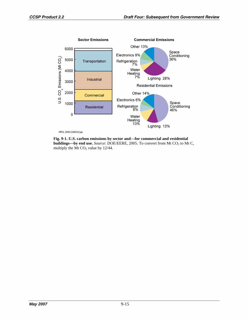
CCSP Product 2.2 Draft Four: Subsequent from Government Review
May 2007 9-15
Fig. 9-1. U.S. carbon emissions by sector and—for commercial and residential buildings—by end use. Source: DOE/EERE, 2005. To convert from Mt CO2 to Mt C, multiply the Mt CO2 value by 12/44.

CCSP Product 2.2 Draft Four: Subsequent from Government Review
May 2007 9-16
[This page intentionally left blank] 1

CCSP Product 2.2 Draft Four: Subsequent from Government Review
May 2007 III-1
PART III OVERVIEW
The Carbon Cycle in Land and Water Systems
Lead Author: R.A. Houghton1
1Woods Hole Research Center
The six chapters (Chapters 10-15) in Part III consider the current and future carbon balance of
terrestrial and aquatic ecosystems in North America. Although the amount of carbon exchanged between
these ecosystems and the atmosphere each year through photosynthesis and plant and microbial
respiration is large, the net balance for all of the ecosystems, combined, is currently a net sink of 370-592
million tons of carbon (Mt C) per year. This net sink offsets only about 20-30% of current fossil-fuel
emissions from the region (1856 Mt C per year in 2003) (see Chapter 3 this report). The cause of this
terrestrial carbon sink is uncertain. Although management has the potential for removing carbon from the
atmosphere and storing it in vegetation and soil, most of the current sink is not the result of current
management practices. Instead, most of it may be attributed to a combination of past management and the
response of terrestrial ecosystems to environmental changes.
The large sink in the forests of Canada and the United States, for example, is, in some measure, the
consequence of continued forest growth following agricultural abandonment that occurred in the past.
This is partly the result of past and current management practices (e.g., fire suppression), and partly the
result of forest responses to a changing environment (climatic change, carbon dioxide [CO2] fertilization,
and the increased mobilization of nutrients). The relative importance of these broad factors in accounting
for the current sink is unknown. Estimates vary from attributing nearly 100% of the sink in United States
forests to regrowth (Caspersen et al., 2000; Hurtt et al., 2002) to attributing nearly all of it to CO2
fertilization (Schimel et al., 2000). The attribution question is critical because the current sink may be
expected to increase in the future if the important mechanism is CO2 fertilization, for example, but may
be expected to decline if the important mechanism is forest regrowth (forests accumulate carbon more
slowly as they age). Understanding the history of land use, management, and disturbance is critical
because disturbance and recovery are major determinants of the net terrestrial carbon flux.
Land-use change and management have been, and will be, important in the carbon balance of other
ecosystems besides forests. The expansion of cultivated lands in Canada and the United States in the
1800s released large amounts of carbon to the atmosphere (Houghton et al., 1999), leaving those lands

CCSP Product 2.2 Draft Four: Subsequent from Government Review
May 2007 III-2
with the potential for recovery (i.e., a future carbon sink), if managed properly. For example, recent
changes in farming practice may have begun to recover the carbon that was lost decades ago. Recovery of
carbon in soil, however, generally takes longer than its loss through cultivation. Grazing lands, although
not directly affected by cultivation, have, nevertheless, been managed in the United States through fire
suppression. The combined effects of grazing and fire suppression are believed to have promoted the
invasion of woody vegetation, possibly a carbon sink at present. Wetlands are also a net carbon sink, but
the magnitude of the sink was larger in the past than it is today, again, as a result of land-use change
(draining of wetlands for agriculture and forestry). The only lands that seem to have escaped management
are those lands overlying permafrost (perennially frozen ground), and they are clearly subject to change in
the future as a result of global warming. Settled lands, by definition, are managed, and are dominated by
fossil-fuel emissions. Nevertheless, the accumulation of carbon in urban and suburban trees suggests a net
sequestration of carbon in the biotic component of long-standing settled lands. Residential lands recently
cleared from forests, on the other hand, are sources of carbon (Wienert and Hamburg, 2006).
From the perspective of carbon and climate, ecosystems are important if (1) they are currently large
sources or sinks of carbon or (2) they have the potential to become large sources or sinks of carbon in the
future through either management or environmental change, where “large” sources or sinks, in this
context, are determined by the product of area (hectares) times flux per unit area (or flux density) (Mg C
per hectare per year).
The largest carbon sink in North America (270 Mt C per year) is associated with forests (Chapter 11
this report) (Table 1). The sink includes the carbon accumulating in wood products (e.g., in increasing
numbers of houses and landfills) as well as in the forests themselves. A sink is believed to exist in
wetlands (Chapter 13 this report), including the wetlands overlying permafrost (Chapter 12 this report),
although the magnitude of this sink is uncertain. More certain is the fact that the current sink is
considerably smaller than it was before wetlands were drained for agriculture and forestry. The other
important aspect of wetlands is that they hold more than half of the carbon in North America. Thus,
despite the current net sink in these systems, their potential for future emissions is large.
Table 1. Ecosystems in North America: their areas, net annual fluxes of carbon (negative values are
sinks), and carbon stocks (including both vegetation and soils)
Although management has the potential to increase the carbon sequestered in agricultural (cultivated)
lands, these lands today are nearly in balance with respect to carbon (Chapter 10 this report). The carbon
lost to the atmosphere from cultivation of organic soils (soils dominated by organic matter) is
approximately balanced by the carbon accumulated in mineral soils (soils consisting of more inorganic

CCSP Product 2.2 Draft Four: Subsequent from Government Review
May 2007 III-3
material, such as sand or clay). In the past, before cultivation, these soils held considerably more carbon
than they do today, but 25-30% of that carbon was lost soon after the lands were initially cultivated. In
large areas of grazing lands, there is the possibility that the invasion and spread of woody vegetation
(woody encroachment) is responsible for a significant net carbon sink at present (Chapter 10 this report).
The magnitude (and even sign) of this flux is uncertain, however, in part because some ecosystems lose
carbon belowground (soils) as they accumulate it aboveground (woody vegetation), and in part because
the invasion and spread of exotic grasses into semi-arid lands of the western United States are increasing
the frequency of fires, reversing woody encroachment, and releasing carbon (Bradley et al., 2006).
The emissions of carbon from settled lands are largely considered in the chapters in Part II and in
Chapter 14 of this report. Non-fossil carbon seems to be accumulating in trees in these lands, but the net
changes in soil carbon are uncertain.
The only ecosystems that appear to release carbon to the atmosphere at present are the coastal waters.
The estimated flux of carbon is close to zero (and difficult to determine) because the gross fluxes (from
river transport, photosynthesis, and respiration) are large and variable in both space and time.
The average net fluxes of carbon expressed as Mg C per hectare per year in Table 1 are for
comparative purposes. They show the relative flux density for different types of ecosystems. These annual
fluxes of carbon are rarely determined with direct measurements of flux, however, because of the extreme
variability of fluxes in time and space, even within a single ecosystem type. Extrapolating from a few
isolated measurements to an estimate for the whole region’s flux is difficult. Rather, the net changes are
more often based on differences in measured stocks over intervals of 10 years, or longer (see Chapter 3
this report), or are based on the large and rapid changes per hectare that are reasonably well documented
for certain forms of management, such as the changes in carbon stocks that result from the conversion of
forest to cultivated land. Thus, most of the flux estimates in Table 1 are long-term and large-area
estimates.
Nevertheless, average flux density is one factor important in determining an ecosystem’s role as a net
source or sink for carbon. The other important factor is area. Permafrost wetlands, for example, are
currently a small net sink for carbon. They cover a large area, however, hold large stocks of carbon, and
thus have the potential to become a significant net source of carbon if the permafrost thaws with global
warming (Smith et al., 2001; Smith et al,. 2005a, Osterkamp and Romanovsky, 1999; Osterkamp et al.,
2000). Forests clearly dominate the net uptake and storage of carbon in North America, although wetlands
and settled lands have mean flux densities that are above average.
The two factors (flux density and area) demonstrate the level of management required to remove a
significant amount of carbon from the atmosphere and keep it on land. Under current conditions,
sequestration of 100 Mt C per year, for example (about 7% of fossil-fuel emissions from North America),

CCSP Product 2.2 Draft Four: Subsequent from Government Review
May 2007 III-4
requires nearly half the forest area (Table 1). As discussed above, the cause of this sequestration is
uncertain, but enhancing it through management over a few hundred million hectares would require
considerable effort. Nevertheless, the cost (in $/metric ton CO2) may be low relative to other options for
managing carbon. For example, forestry activities are estimated to have the potential to sequester 100-200
Mt C per year in the United States at prices ranging from less than $10/ton of CO2 for improved forest
management, to $15/ton for afforestation, to $30-50/ton for production of biofuels (Chapter 11 this
report). Somewhat smaller sinks of 10-70 Mt C per year might be stored in agricultural soils at low to
moderate costs ($3-30/ton CO2) (Chapter 10 this report). The maximum amounts of carbon that might be
accumulated in forests and agricultural soils are not known, thus, the number of years these rates of
sequestration might be expected to continue is also unknown. It seems unlikely that the amount of carbon
currently held in forests and agricultural lands could double. Changes in climate will also affect carbon
storage, but the net effect of management and climate is uncertain.
Despite the limited nature of carbon uptake and storage in offsetting the global emissions of carbon
from fossil fuels, local and regional activities may, nevertheless, offset local and regional emissions of
fossil carbon. This offset, as well as other co-benefits, may be particularly successful in urban and
suburban systems (Chapter 14 this report).
The effects and cost of managing aquatic systems are less clear. Increasing the area of wetlands, for
example, would presumably increase the sequestration of carbon; but it would also increase emissions of
methane (CH4), countering the effect of carbon storage. Fertilization of coastal waters with iron has been
proposed as a method for increasing oceanic uptake of CO2, but neither the amount of carbon that might
be sequestered nor the side effects are known (Chapter 15 this report).
A few studies have estimated the potential magnitudes of future carbon sinks as a result of
management (Chapters 10, 11 this report). However, the contribution of management, as opposed to the
environment, in today’s sink is unclear (see Chapter 3 this report), and for the future, the relative roles of
management and environmental change are even less clear. The two drivers might work together to
enhance terrestrial carbon sinks, as seems to have been the case during recent decades (Prentice et al.,
2001) (Chapter 2 this report). On the other hand, they might work in opposing directions. A worst-case
scenario, quite possible, is one in which management will become ineffective in the face of large natural
sources of carbon not previously experienced in the modern world. In other words, while management is
likely to be essential for sequestering carbon, it may not be sufficient to preserve the current terrestrial
carbon sink over North America, let alone to offset fossil-fuel emissions.
At least one other observation about storing carbon in terrestrial and aquatic ecosystems should be
mentioned. In contrast to the hundreds of millions of hectares that must be managed to sequester 100 Mt
C annually, a few million hectares of forest fires can release an equivalent amount of carbon in a single

CCSP Product 2.2 Draft Four: Subsequent from Government Review
May 2007 III-5
year. This disparity in flux densities underscores the fact that a few million hectares are disturbed each
year, while hundreds of millions of hectares are recovering from past disturbances. The natural fluxes of
carbon are large in comparison to net fluxes. The observation is relevant for carbon management, because
the cumulative effects of managing small net sinks to mitigate fossil-fuel emissions will have to be
understood, analyzed, monitored, and evaluated in the context of larger, highly variable, and uncertain
sources and sinks in the natural cycle.
The major challenge for future research is quantification of the mechanisms responsible for current
(and future) fluxes of carbon. In particular, what are the relative effects of management (including land-
use change), environmental change, and natural disturbance in determining sources and sinks of carbon
for today and tomorrow? Will the current natural sinks continue, grow in magnitude, or reverse to become
net sources? What is the role of soils in the current (and future) carbon balance (Davidson and Janssens,
2006)? What are the most cost-effective means of managing carbon?
Answering these questions will require two scales of measurement: (1) an expanded network of
intensive research sites dedicated to understanding basic processes (e.g., the effects of management and
environmental effects on carbon stocks), and (2) extensive national-level networks of monitoring sites,
through which uncertainties in carbon stocks (inventories) would be reduced and changes, directly
measured. Elements of these measurements are underway, but the effort has not yet been adequate for
resolving these questions.
KEY UNCERTAINTIES AND GAPS IN UNDERSTANDING THE CARBON CYCLE OF NORTH AMERICA • As mentioned above, the net flux of carbon resulting from woody encroachment and its inverse,
woody elimination, is highly uncertain. Even the sign of the flux is in question.
• Rivers, lakes, dams, and other inland waters are mentioned in Chapter 15 as being a source of carbon,
but they are claimed elsewhere to be a sink (Chapter 3 this report). The sign of the net carbon flux
attributable to erosion, transport, deposition, accumulation, and decomposition is uncertain (e.g.,
Stallard, 1998; Lal, 2001; Smith et al., 2005b).
• Several chapters cite studies that have attempted to quantify the potential for management to increase
carbon sinks in the future, but no studies have yet attempted to estimate the potential future sources of
carbon for North America as they have for the globe (e.g., Friedlingstein et al., 2006; Jones et al.,
2005). Global models that include the feedbacks between climatic change and the carbon cycle have
all shown decreased carbon sinks over the next century. In North America, warming of wetlands and
thawing of permafrost, in particular, are likely to increase emissions of carbon to the atmosphere, CH4
as well as CO2; and periods of unusually low rainfall, combined with warming trends, are likely to

CCSP Product 2.2 Draft Four: Subsequent from Government Review
May 2007 III-6
release carbon from the ecosystems of the Mountain West and the southwestern United States through
increasing their vulnerability to wildfires and insect outbreaks (Potter et al., 2003, 2005).
REFERENCES FOR PART III OVERVIEW
Bradley, B.A., R.A. Houghton, J.F. Mustard, and S.P. Hamburg, 2006: Invasive grass reduces aboveground carbon
stocks in shrublands of the Western US. Global Change Biology, 12, 1815-1822.
Caspersen, J.P., S.W. Pacala, J.C. Jenkins, G.C. Hurtt, P.R. Moorcroft, and R.A. Birdsey, 2000: Contributions of
land-use history to carbon accumulation in United States forests. Science, 290, 1148-1151.
Davidson, E.A., and I.A. Janssens, 2006: Temperature sensitivity of soil carbon decomposition and feedbacks to
climate change. Nature, 440, 165-173.
Friedlingstein, P., P. Cox, R. Betts, L. Bopp, W. von Bloh, V. Brovkin, P. Cadule, S. Doney, M. Eby, I. Fung, G.
Bala, J. John, C. Jones, F. Joos, T. Kato, M. Kawamiya, W. Knorr, K. Lindsay, H.D. Matthews, T. Raddatz, P.
Rayner, C. Reick, E. Roeckner, K.-G. Schnitzler, R. Schnur, K. Strassmann, A.J. Weaver, C. Yoshikawa, and
N. Zeng, 2006: Climate-carbon cycle feedback analysis: results from the C4MIP model intercomparison.
Journal of Climate, 19, 3337-3353.
Houghton, R.A., J.L. Hackler, and K.T. Lawrence, 1999: The United States carbon budget: contributions from land-
use change. Science, 285, 574-578.
Hurtt, G.C., S.W. Pacala, P.R. Moorcroft, J. Caspersen, E. Shevliakova, R.A. Houghton, and B. Moore III, 2002:
Projecting the future of the United States carbon sink. Proceedings of the National Academy of Sciences, 99,
1389-1394.
Jones, C., C. McConnell, K. Coleman, P. Cox, P. Falloon, D. Jenkinson, and D. Powlson, 2005: Global climate
change and soil carbon stocks; predictions from two contrasting models for the turnover of organic carbon in
soil. Global Change Biology, 11, 154-166.
Lal, R., 2001: Fate of eroded soil carbon: emission or sequestration. In: Soil Carbon Sequestration and the
Greenhouse Effect [R. Lal (ed.)]. Soil Science Society of America Special Publication, vol. 57; Madison,
Wisconsin, pp. 173-181.
Osterkamp, T.E., and V.E. Romanovsky, 1999: Evidence for warming and thawing of discontinuous permafrost in
Alaska. Permafrost and Periglacial Processes, 10(1), 17-37.
Osterkamp, T.E., L. Viereck, Y. Shur, M.T. Jorgenson, C. Racine, A. Doyle, and R.D. Boone, 2000: Observations
of thermokarst and its impact on boreal forests in Alaska, United States. Arctic, Antarctic and Alpine Research,
32, 303-315.
Potter, C., P. Tan, V. Kumar, C. Kucharik, S. Klooster, V. Genovese, W. Cohen, and S. Healey, 2005. Recent
history of large-scale ecosystem disturbances in North America derived from the AVHRR satellite record.
Ecosystems, 8, 808.
Potter, C., S. Klooster, P. Tan, M. Steinbach, V. Kumar, and V. Genovese, 2003: Variability in terrestrial carbon
sinks over two decades: Part 1—North America. Earth Interactions, 7, Paper 12.
CCSP Product 2.2 Draft Four: Subsequent from Government Review
May 2007 III-7
Prentice, I.C., G.D. Farquhar, M.J.R. Fasham, M.L. Goulden, M. Heimann, V.J. Jaramillo, H.S. Kheshgi, C. Le
Quéré, R.J. Scholes, and D.W.R. Wallace, 2001: The carbon cycle and atmospheric carbon dioxide. In: Climate
Change 2001: The Scientific Basis. Contribution of Working Group I to the Third Assessment Report of the
Intergovernmental Panel on Climate Change [J. T. Houghton, Y. Ding, D. J. Griggs, M. Noguer, P. J. van der
Linden, X. Dai, K. Maskell, and C. A. Johnson (eds.)]. Cambridge University Press, Cambridge, UK and New
York, NY, United States, pp. 183-237.
Schimel, D., J. Melillo, H. Tian, A.D. McGuire, D. Kicklighter, T. Kittel, N. Rosenbloom, S. Running, P. Thornton,
D. Ojima, W. Parton, R. Kelly, M. Sykes, R. Neilson, and B. Rizzo, 2000: Contribution of increasing CO2 and
climate to carbon storage by ecosystems in the United States. Science, 287, 2004-2006.
Smith, L.C., Y. Sheng, G.M. MacDonald, L.D. Hinzman, 2005a: Disappearing Arctic Lakes. Science, 308, 1429.
Smith, S.L., M.M. Burgess, and F.M. Nixon, 2001: Response of activelayer and permafrost temperatures to
warming during 1998 in the Mackenzie Delta, Northwest Territories and at Canadian Forces Station Alert and
Baker Lake, Nunavut. Geological Survey of Canada Current Research, 2001-E5, 8 pp.
Smith, S.V., R.O. Sleezer, W.H. Renwick, and R.W. Buddemeier, 2005b: Fates of eroded soil organic carbon:
Mississippi Basin case study. Ecological Applications, 15, 1929-1940.
Stallard, R.F., 1998: Terrestrial sedimentation and the carbon cycle: Coupling weathering and erosion to carbon burial.
Global Biogeochemical Cycles, 12, 231-257.
Wienert, A., and S.P. Hamburg, 2006: Carbon stock changes and greenhouse gas emissions from exurban land
development in central New Hampshire. Master’s Thesis, Brown University, Providence, Rhode Island.

CCSP Product 2.2 Draft Four: Subsequent from Government Review
May 2007 III-8
Table 1. Ecosystems in North America: their areas, net annual fluxes of carbon (negative values are sinks), and carbon stocks (including both vegetation and soils)
Type of ecosystem
Area (106 ha)
Current mean flux density
(Mg C ha–1 yr–1)
Current flux
(Mt C yr–1)
Carbon stocks (Mt C)
Mean carbon stocks (Mt C ha–1)
Agriculture 231 0.0 0±151 18,500 80 Grass, shrub and arid 558 –0.01 –62 59,950 107 Forests 771 –0.35 –2693 171,500 222 Permafrost lands Peatlands 51 –0.13 –6.7 57,700 1130 Mineral soils4 517 –0.03 –14 98,780 191 Non-permafrost wetlands Peatlands 86 –0.12 –10 126,400 1470 Mineral soils 105 –0.21 –22.3 38,100 363 Estuarine 4.5 –2.3 –10.2 900 200 Settled lands 104 –0.315 –325 ~1,0005 10 Coastal waters 384 0.05 19
Sum 24276 –0.157 –3708 572,8306
Total 21269 480,00010 2257
1. Fossil fuel inputs to crop management are not included. Some of the carbon sequestration is occurring on
grasslands as well as croplands, but the inventories do not separate these fluxes. The near-zero flux is for Canada and the United States only. Including Mexican croplands would likely change the flux to a net source because croplands are expanding in Mexico, and the carbon in biomass and soil is released to the atmosphere as native ecosystems are cultivated.
2. Fossil fuels are not included. The small net sink results from the Conservation Reserve Program in the United States Including Mexico is likely to change the net sink to a source because forests are being converted to grazing lands. Neither woody encroachment nor woody elimination is included in this estimate of flux because the uncertainties are so large.
3. Includes an annual sink of 68 Mt C yr–1 in wood products as well as a sink of 201 Mt C yr–1 in forested ecosystems.
4. Includes zones with continuous, discontinuous, sporadic, and isolated permafrost; that is, not all of the lands are strictly over permafrost.
5. Urban trees only (does not include soil carbon). 6. Sum does not include coastal waters. The summed area is larger than the total area (note 9) because of
double counting. For example, an estimated 75 × 106 ha of permafrost lands in Canada are forested (and may be included in forest area as well as permafrost area), 26 x 106 ha of wetlands in the U.S. are forested, and 54 x 106 ha of wetlands are shrublands. In addition, an estimated 75 x 106 ha of other wooded lands are included as both forests and rangelands, and ~70 x 106 ha of grasslands and shublands are counted also as non-permafrost lands within areas defined as sporadic or isolated permafrost (see note 4).
7. Weighted average; does not include coastal waters. 8. Does not include coastal waters. The total annual sink of 370 Mt C is lower than the estimate of 592 Mt C
presented in Chapter 3 (Table 3-1). The largest difference results from the flux of carbon attributed to woody encroachment. Chapter 3 includes a sink of 120 Mt C yr–1; Table 1, above, presents a net flux of zero (see note 2). Other differences between the two estimates include: (1) an additional sink in Table 1 of 14 Mt C yr–1 in permafrost mineral soils; (2) an additional sink in Table 1 of 32 Mt C yr–1 in settled lands; and (3) a sink of 25 Mt C yr–1 in rivers and reservoirs that is included in Table 3-1 but not in Table 1. In addition, there are small differences in the estimates for agricultural lands and grasslands.
9. Areas (106 ha) (The Times Atlas of the World, 1990) Globe North America Canada United States Mexico
14,900 2,126 992 936 197 10. Total carbon stocks are reduced by the areas double counted (see note 6).
CCSP Product 2.2 Draft Four: Subsequent from Government Review
May 2007 10-1
Chapter 10. Agricultural and Grazing Lands
Lead Authors: Richard T. Conant1 and Keith Paustian1,2
Contributing Authors: Felipe García-Oliva,3 H. Henry Janzen,4 Victor J. Jaramillo,3
Donald E. Johnson,5 and Suren N. Kulshreshtha6
1Natural Resource Ecology Laboratory, Colorado State University,
2Department of Soil and Crop Science, Colorado State University, 3Centro de Investigaciones en
Ecosistemas, Universidad Nacional Autónoma de México, 4Environmental Health, Agriculture and Agri-Food
Canada, 5Department of Animal Science, Colorado State University (deceased), 6Department of Agricultural
Economics, University of Saskatchewan
KEY FINDINGS
• Agricultural and grazing lands (cropland, pasture, rangeland, shrublands, and arid lands) occupy 789
million hectares (1.95 billion acres), which is 47% of the land area of North America, and contain
78.5±19.51 billion tons of carbon (17% of North American terrestrial carbon) in the soil alone.
• The emissions and uptake and storage of carbon on agricultural lands are mainly determined by two
conditions: management and changes in the environment. The effects of converting forest and
grassland to agricultural lands and of agricultural management (e.g., cultivation, conservation tillage)
are reasonably well known and have been responsible for historic losses of carbon in Canada and the
United States (and for current losses in Mexico); the effects of climate change or of elevated
concentrations of atmospheric carbon dioxide are uncertain.
• Conservation-oriented management of agricultural lands (e.g., use of conservation tillage, improved
cropping and grazing systems, reduced bare fallow, set-asides of fragile lands, and restoration of
degraded soils) can significantly increase soil carbon stocks.
• Agricultural and grazing lands in the United States and Canada are currently near neutral with respect
to their soil carbon balance, but agricultural and grazing lands in Mexico are likely losing carbon due
to land use change. Although agricultural soils are estimated to currently uptake about 19-20 million
tons of carbon per year, the cultivation of organic soils releases approximately 6-12 million tons of
carbon per year. On-farm fossil-fuel use (around 31 million tons of carbon per year), agricultural
liming (1.2 million tons carbon per year), and manufacture of agricultural inputs including fertilizer
(approximately 6 million tons of carbon per year) yields a net source from the agricultural sector of
about 25-30 million tons of carbon per year. 1 The uncertainty in this value is given as one standard error.

CCSP Product 2.2 Draft Four: Subsequent from Government Review
May 2007 10-2
• As much as 120 million tons of carbon per year may be accumulating through woody encroachment
of arid and semi-arid lands of North America; this value is highly uncertain. Woody encroachment is
generally accompanied by decreased forage production, and ongoing efforts to reestablish forage
species are likely to reverse carbon accumulation by vegetation.
• Projections of future trends in agricultural land area and soil carbon stocks are unavailable or highly
uncertain because of uncertainty in future land-use change and agricultural management practice.
• Annualized prices of $15/metric ton carbon dioxide, could yield mitigation amounts of 46 million tons
of carbon per year captured in agricultural soils and 14.5 million tons of carbon per year from
reductions in fossil-fuel use. At lower prices of $5/metric ton carbon dioxide, the corresponding values
would be 34 million tons of carbon per year and 9 million tons of carbon per year, respectively.
• Policies designed to suppress emissions of one greenhouse gas need to consider complex
interactions to ensure that net emissions of total greenhouse gases are reduced. For example,
increased use of fertilizer or irrigation may increase crop residues and carbon uptake and storage, but
may stimulate emissions of methane or nitrous oxide.
• Many of the practices that lead to carbon capture and storage or to reduced carbon dioxide and
methane emissions from agricultural lands not only increase production efficiencies, but lead to
environmental co-benefits, for example, improved soil fertility, reduced erosion and pesticide
immobilization.
• An expanded network of intensive research sites would allow us to better understand the effects of
management on carbon cycling and storage in agricultural systems. An extensive national-level
network of soil monitoring sites in which changes in carbon stocks are directly measured would allow
us to reduce the uncertainty in the inventory of agricultural and grazing land carbon. Better
information about the spatial extent of woody encroachment, the amount and growth of woody
vegetation, and variation in impacts on soil carbon stocks would help reduce the large uncertainty of
the carbon impacts of woody encroachment.
1. INVENTORY
1.1 Background
Agricultural and grazing lands (cropland, pasture, rangeland, shrublands, and arid lands2) occupy
47% of the land area in North America (59% in the United States, 70% in Mexico, and 11% in Canada),
and contain 17% of the terrestrial carbon. Most of the carbon in these ecosystems is held in soils. Live
vegetation in cropland generally contains less than 5% of total carbon, whereas vegetation in grazing
2We refer collectively to pasture, rangeland, shrublands, and arid lands as grazing lands since grazing is their primary use,
even though not all of these lands are grazed.
CCSP Product 2.2 Draft Four: Subsequent from Government Review
May 2007 10-3
lands contains a greater proportion (5–30%), but still less than that in forested systems (30–65%).
Agricultural and grazing lands in North America contain 78.5±19.5 (±1 standard error) billion tons of
carbon (Gt C) in the soil (Table 10-1). Significant increases in vegetation carbon stocks in some grazing
lands have been observed and, together with soil carbon stocks from croplands and grazing lands, likely
contribute significantly to the large North American terrestrial carbon sink (Houghton et al., 1999; Pacala
et al., 2001; Eve et al., 2002; Ogle et al., 2003). These lands also emit greenhouse gases: fossil-fuel use
for on-farm machinery and buildings, for manufacture of agricultural inputs, and for transportation
account for 3–5% of total carbon dioxide (CO2) emissions in developed countries (Enquete Commission,
1995); activities on agricultural and grazing lands, like livestock production, animal waste management,
biomass burning, and rice cultivation, emit 35% of global anthropogenic methane (CH4) (27% of United
States, 31% of Mexican, and 27% of Canadian CH4 emissions) (Mosier et al., 1998b; CISCC, 2001;
Ministry of the Environment, 2006; EPA, 2006); and agricultural and grazing lands are the largest
anthropogenic source of nitrous oxide (N2O) emissions (CAST, 2004; see Text Box 1). However,
agricultural and grazing lands are actively managed and have the capacity to take up and store carbon.
Thus improving management could lead to substantial reductions in CO2 and CH4 emissions and could
sequester carbon to offset emissions from other lands or sectors.
Table 10-1. Soil carbon pools in agricultural and grazing lands in Canada, Mexico, and the United
States.
1.2 Carbon Dioxide Fluxes from Agricultural and Grazing Land
The main processes governing the carbon balance of agricultural and grazing lands are the same as
for other ecosystems: the photosynthetic uptake and assimilation of CO2 into organic compounds and the
release of gaseous carbon through respiration (primarily CO2 but also CH4) and fire. Like other terrestrial
ecosystems in general, for which CO2 emissions are approximately two orders of magnitude greater than
CH4 emissions, carbon cycling in most agricultural and grazing lands is dominated by fluxes of CO2
rather than CH4. In agricultural lands, carbon assimilation is directed towards production of food, fiber,
and forage by manipulating species composition and growing conditions (soil fertility, irrigation, etc.).
Biomass, being predominantly herbaceous (i.e., non-woody), is a small, transient carbon pool (compared
to forests) and hence soils constitute the dominant carbon stock. Cropland systems can be among the most
productive ecosystems, but in some cases restricted growing season length, fallow periods, and grazing-
induced shifts in species composition or production can reduce carbon uptake relative to that in other
ecosystems. These factors, along with tillage-induced soil disturbances and removal of plant carbon
through harvest, have depleted soil carbon stocks by 20-40% or more from pre-cultivated conditions

CCSP Product 2.2 Draft Four: Subsequent from Government Review
May 2007 10-4
(Davidson and Ackerman, 1993; Houghton and Goodale, 2004). Soil organic carbon stocks in grazing
lands (see Text Box 2 for information on inorganic soil carbon stocks) have been depleted to a lesser
degree than for cropland (Ogle et al., 2004), and in some regions biomass has increased due to
suppression of disturbance and subsequent woody encroachment (see Text Box 3). Woody encroachment
is potentially a significant sink for atmospheric CO2, but the magnitude of the sink is poorly constrained
(Houghton et al., 1999; Pacala et al., 2001). Since woody encroachment leads to decreased forage
production, management practices are aimed at reversing it, with consequent reductions in biomass
carbon. Disturbance-induced increases in decomposition rates of aboveground litter and harvest removal
of some (30–50% of forage in grazing systems, 40–50% in grain crops) or all (e.g., corn for silage) of the
aboveground biomass, have drastically altered carbon cycling within agricultural lands and thus the
sources and sinks of CO2 to the atmosphere.
Much of the carbon lost from agricultural soil and biomass pools can be recovered with changes in
management practices that increase carbon inputs, stabilize carbon within the system, or reduce carbon
losses, while still maintaining outputs of food, fiber, and forage. Increased production, increased residue
C inputs to the soil, and increased organic matter additions have reversed historic soil C losses in long-
term experimental plots (e.g., Buyanovsky and Wagner, 1998). However, the management practices that
promote soil carbon sequestration would need to be maintained over time to avoid subsequent losses of
sequestered carbon. Across Canada and the United States, mineral soils have been sequestering 2.5 and
17.0 ± 0.45 million tons of carbon (Mt C) per year† (Ministry of the Environment, 2006; Ogle et al., 2003;
EPA, 2006), respectively, largely through increased production and improved management practices on
annual cropland (Fig. 10-1, Table 10-2). Conversion of agricultural land to grassland, like under the
Conservation Reserve Program in the United States (7.6–11.5 Mt C per year on 31.5 million acres [12.5
million hectares] of land), and afforestation have also sequestered carbon in agricultural and grazing lands
(Follett et al., 2001a). In contrast, cultivation of organic soils (e.g., peat-derived soils) is releasing an
estimated 0.1 and 8.3 ± 3.2 Mt C per year† from soils in Canada and the United States (Matin et al., 2004;
Ministry of the Environment, 2006; Ogle et al., 2003; EPA, 2006). Compared with other systems, the
high productivity and management-induced disturbances of agricultural systems promote movement and
redistribution (through erosion, runoff and leaching) of organic and inorganic carbon, sequestering
potentially large amounts of carbon in sediments and water (Raymond and Cole, 2003; Smith et al. 2005;
Yoo et al., 2005). However, the net impact of soil erosion on carbon emissions to the atmosphere remains
highly uncertain.
† The magnitude and/or range of uncertainty for the given numerical value(s) is not provided in the references cited.

CCSP Product 2.2 Draft Four: Subsequent from Government Review
May 2007 10-5
Figure 10-1. North American agricultural and grazing land CO2 (left side) and methane (right side),
adjusted for global warming potential.
Table 10-2. North American agricultural and grazing land carbon fluxes for the years around 2000
Production, delivery, and use of field equipment, fertilizer, seed, pesticides, irrigation water, and
maintenance of animal production facilities contribute 3–5% of total fossil-fuel CO2 emissions in
developed countries (Enquete Commission, 1995). On-farm fossil-fuel emissions together with
manufacture of fertilizers and pesticides contribute emissions of 32.7 Mt C per year† within the United
States (Lal et al., 1998) and 4.6 Mt C per year in Canada (Kulshreshtha et al., 2000) (Table 10-2). Energy
consumption for heating and cooling high intensity animal production facilities is among the largest CO2
emitters within the agricultural sector (Enquete Commission, 1995).
Much of the ammonia production and urea application (U.S.: 4.3 Mt C per year; Mexico: 0.4 Mt C
per year; Canada: 1.7 Mt C per year) and phosphoric acid manufacture (U.S.: 0.4 Mt C per year; Mexico:
0.2 Mt C per year; Canada: not reported) are devoted to agricultural uses.
1.3 Methane Fluxes from Agricultural and Grazing Lands
Cropland and grazing land soils act as both sources and sinks for atmospheric CH4. Methane
formation is an anaerobic process and is most significant in waterlogged soils, like those under paddy rice
cultivation (U.S.: 0.25 ± 0.28 Mt CH4-C per year; Mexico: 0.01 Mt CH4-C per year;† Canada: negligible,
not reported; Table 10-2). Methane is also formed by incomplete biomass combustion of crop residues
(U.S.: 0.03 ± 0.02 Mt CH4-C per year; Mexico: <0.01 Mt CH4-C per year; Canada: negligible, not
reported; Table 10-2). Methane oxidation in soils is a global sink for about 5% of CH4 produced annually
and is mainly limited by CH4 diffusion into the soil. However, intensive cropland management tends to
reduce soil methane consumption relative to forests and extensively grazing lands (CAST, 2004).
Management-induced changes in CH4-C fluxes have a smaller impact on terrestrial carbon cycling than
changes in CO2-C fluxes (Table 10-2), but relatively greater radiative forcing for CH4 amplifies the
impact of increasing atmospheric CH4 concentrations on net radiative forcing (Fig. 10-1). Recent research
has shown that live plant biomass and litter produce substantial amounts of CH4, potentially making
plants as large a source of CH4 as livestock (Keppler et al., 2006). If this is the case, activities that
increase plant biomass—and sequester CO2—may lead to increased CH4 production (Keppler et al.,
2006).
CCSP Product 2.2 Draft Four: Subsequent from Government Review
May 2007 10-6
1.4 Methane Fluxes from Livestock
Enteric fermentation (the process of organic matter breakdown by gut flora within the gastrointestinal
tract of animals, particularly ruminants) allows for the digestion of fibrous materials by livestock, but the
extensive fermentation of the ruminant diet requires 5–7% of the dietary gross energy to be belched out as
CH4 to sustain the anaerobic processes (Johnson and Johnson, 1995). Methane emissions from livestock
contribute significantly to total CH4 emissions in the United States (3.7 ± 0.53 Mt CH4-C per year, 20% of
total U.S. CH4 emissions), Canada (0.78 ± 0.14 Mt CH4-C per year, 22% of total) (Ministry of the
Environment, 2006; Sobool and Kulshreshtha, 2005), and Mexico (1.5 Mt CH4-C per year, 27% of total)†
with the vast majority of enteric CH4 emissions are from beef (72%) and dairy cattle (23%) (Table 10-2).
Emissions from ruminants are tightly coupled to feed consumption, since CH4 emission per unit of feed
energy is relatively constant, except for feedlot cattle with diets high in cereal grain contents, for which
the fractional loss falls to one-third to one-half of normal rates (Johnson and Johnson, 1995). Between
1990 and 2002, CH4 emissions from enteric fermentation fell 2% in the United States but increased by
20% in Canada (EPA, 2000; Matin et al., 2004).
Methane emissions during manure storage (U.S.: 1.3 ± 0.24 Mt CH4 per year; Mexico: 0.06 Mt CH4
per year;† Canada: 0.3 ± 0.05 Mt CH4 per year) are governed by the amount of degradable organic matter,
degree of anoxia, storage temperature, and duration of storage. Unlike enteric CH4, the major sources of
manure CH4 emissions in the United States are from swine (44%) and dairy cattle (39%). Manure CH4
production is greater for production systems with anoxic lagoons, largely anoxic pits, or manure handled
or stored as slurry. Between 1990 and 2002, CH4 emissions from manure management increased 25% in
the United States and 21% in Canada (EPA, 2000; Matin et al., 2004).
2. DRIVERS AND TRENDS
The extent to which agricultural options will contribute to greenhouse gas mitigation will largely
depend on government policy decisions, but mitigation opportunities will also be constrained by
technological advances and changing environmental conditions (see discussion below). Estimates from
national inventories suggest that U.S. and Canadian agricultural soils are currently near neutral or small
net sinks for CO2, which has occurred as a consequence of changing management (e.g., reduced tillage
intensity) and government programs designed for purposes other than greenhouse gas mitigation (e.g.,
soil conservation, commodity regulation). However, to realize the much larger potential for soil carbon
sequestration (see section below) and for significant reductions in CH4 (and N2O) emissions, specific
policies targeted at greenhouse gas reductions are required. It is generally recognized that farmers (and
other economic actors) are, as a group, ‘profit-maximizers,’ which implies that to change from current
practices to ones that reduce net emissions, farmers will incur additional costs (termed ‘opportunity cost’).

CCSP Product 2.2 Draft Four: Subsequent from Government Review
May 2007 10-7
Hence, where the incentives (e.g., carbon offset market payments, government subsidies) to adopt new
practices exceed the opportunity costs, farmers will adopt new practices. Crop productivity, production
input expenses, marketing costs, etc. (which determine profitability) vary widely within (and between)
countries. Thus, the payment needed to achieve a unit of emission reduction will vary, among and within
regions. In general, each successive increment of carbon sequestration or emission reduction comes at a
progressively higher cost (this relationship is often shown in the form of an upward bending marginal cost
curve).
The interaction of changes in technological and environmental conditions, including crop growth
improvements, impacts of CO2 increase, N deposition, and climate change, will shape future trends in
greenhouse gas emissions and mitigation from agricultural and grazing lands. A continuation of the yield
increases seen in the past several decades for agricultural crops (Reilly and Fuglie, 1998) would tend to
enhance the potential for soil C sequestration (CAST, 2004). Similarly, increased plant growth due to
higher concentrations of CO2 (and N deposition) has been projected to boost carbon uptake on
agricultural (and other) lands, offsetting some or all of the climate-change induced reductions in
productivity projected in some regions of North America (NAS, 2001). However, recent syntheses from
field-scale FACE (Free-Air Carbon dioxide Enrichment) studies of croplands (Long et al., 2006) and
grasslands (Nowak et al., 2004) suggest that the growth enhancement from CO2 fertilization may be much
less than previously thought. Feedbacks between temperature and soil carbon stocks could counteract
efforts to reduce greenhouse gases via carbon sequestration within agricultural ecosystems. Increased
temperatures tend to increase the rate of biological processes—including plant respiration and organic
matter decay and CO2 release by soil organisms—particularly in temperate climates that prevail across
most of North America. Because soil carbon stocks, including those in agricultural lands, contain such
large amounts of carbon, small percentage increases in rate of soil organic matter decomposition could
lead to substantially increased emissions (Jenkinson et al., 1991; Cox et al., 2000). There is currently a
scientific debate about the relative temperature sensitivity of the different constituents making up soil
organic matter (e.g., Kätterer et al., 1998; Giardina and Ryan, 2000; Ågren and Bosatta, 2002; Knorr et
al., 2005), reflecting uncertainty in the possible degree and magnitude of climate change feedbacks.
Despite this uncertainty, the potential for climate and other environmental feedbacks to influence the
carbon balance of agricultural systems by perturbing productivity (and carbon input rates) and organic
matter turnover, and potentially soil N2O and CH4 fluxes, cannot be overlooked.

CCSP Product 2.2 Draft Four: Subsequent from Government Review
May 2007 10-8
3. OPTIONS FOR MANAGEMENT
3.1 Carbon Sequestration
Agricultural and grazing land management practices capable of increasing carbon inputs or
decreasing carbon outputs, while still maintaining yields, can be divided into two classes: those that
impact carbon inputs, and those that affect carbon release through decomposition and disturbance.
Reversion to native vegetation or setting agricultural land aside as grassland, such as in the Canadian
Prairie Cover Program and the U.S. Conservation Reserve Program, can increase the proportion of
photosynthesized carbon retained in the system and sequester carbon in the soil3 (Conant et al., 2001; Post
and Kwon, 2000; Follett et al., 2001b) (Fig. 10-2). In annual cropland, improved crop rotations, yield
enhancement measures, organic amendments, cover crops, improved fertilization and irrigation practices,
and reduced bare fallow tend to increase productivity and carbon inputs, and thus soil carbon stocks (Lal
et al., 1998; Paustian et al., 1998; VandenBygaart et al., 2003) (Fig. 10-2). Tillage, traditionally used for
soil preparation and weed control, disturbs the soil and stimulates decomposition and loss of soil carbon.
Practices that substantially reduce (reduced-till) or eliminate (no-till) tillage-induced disturbances are
being increasingly adopted and generally increase soil carbon stocks while maintaining or enhancing
productivity levels (Paustian et al,. 1997; Ogle et al., 2003) (Fig. 10-2). Estimates of the technical
potential for annual cropland soil carbon sequestration are on the order of 50–100 Mt C per year† in the
United States (Lal et al., 2003; Sperow et al., 2003) and 3.3–6.4 Mt C per year† in Canada (Boehm et al.,
2004).
Figure 10-2. Relative soil carbon following implementation of new agricultural or grassland
management practices.
Within grazing lands, historical overgrazing has substantially reduced productive capacity in many
areas, leading to loss of soil carbon stocks (Conant and Paustian, 2002) (Fig. 10-2). Conversely, improved
grazing management and production inputs—like fertilizer, adding (N-fixing) legumes, organic
amendments, and irrigation—can increase productivity, carbon inputs, and soil carbon stocks (Conant et
al., 2001), potentially storing 0.44 Mt C per year† in Canada (Lynch et al., 2005) and as much as 16–54
(mean = 33.2) Mt C per year in the United States (Follett et al., 2001a). Such improvements will carry a
3The bulk of carbon sequestration potential in agricultural and grazing lands is restricted to soil carbon pools, though carbon
can be sequestered in woody biomass in agroforestry systems (Sheinbaum and Masera, 2000). Woody encroachment on grasslands can also store substantial amounts of carbon in biomass, but the phenomenon is neither well-controlled nor desirable from the standpoint of livestock production, since it results in decreased forage productivity, and the impacts on soil carbon pools are highly variable and poorly understood.

CCSP Product 2.2 Draft Four: Subsequent from Government Review
May 2007 10-9
carbon cost, particularly fertilization and irrigation since their production and implementation require the
use of fossil fuels.
3.2 Fossil-Fuel Derived Emission Reductions
The efficiency with which on-farm (from tractors and machinery) and off-farm (from production of
agricultural input) energy inputs are converted to agricultural products varies several-fold (Lal, 2004).
Where more energy-efficient practices can be substituted for less efficient ones, fossil-fuel CO2 emissions
can be reduced (Lal, 2004). For example, converting from conventional plowing to no-tillage can reduce
on-farm fossil-fuel emissions by 25–80% (Frye, 1984; Robertson et al., 2000) and total fossil-fuel
emissions by 14–25% (West and Marland, 2003). Substitution of legumes for mineral nitrogen can reduce
energy input by 15% in cropping systems incorporating legumes (Pimentel et al., 2005). More efficient
heating and cooling (e.g., better building insulation) could reduce CO2 emissions associated with housed
animal (e.g., dairy) facilities. Substitution of crop-derived for fossil fuels could decrease net emissions.
Energy intensity (energy per unit product) for the U.S. agricultural sector has declined since the 1970s
(Paustian et al., 1998). Between 1990 and 2000, fossil-fuel emissions on Canadian farms increased by
35%† (Sobool and Kulshreshtha, 2005).
3.3 Methane Emission Reduction
Reducing flood duration and decreasing organic matter additions to paddy rice fields can reduce CH4
emissions. Soil amendments such as ammonium sulfate and calcium carbide inhibit CH4 formation.
Coupled with adoption of new rice cultivars that favor lower CH4 emissions, these management practices
could reduce CH4 emission from paddy rice systems by 16–70% (mean = 40%) of current emissions
(Mosier et al., 1998b).
Biomass burning is uncommon in most Canadian and U.S. crop production systems; less than 3% of
crop residues are burned annually in the United States (EPA, 2006). Biomass burning in conjunction with
land clearing and with subsistence agriculture still occurs in Mexico, but these practices are declining.
The primary path for emission reduction is reducing residue burning (CAST, 2004).
Refinement of feed quality, feed rationing, additives, and livestock production efficiency chains can
all reduce CH4 emissions from ruminant livestock with minimal impacts on productivity or profits
(CAST, 2004). Boadi et al. (2004) review several examples of increases in energy intensity. Wider
adoption of more efficient practices could reduce CH4 production from 5–8% to 2–3% of gross feed
energy (Agriculture and Agri-Food Canada, 1999), reducing CH4 emissions by 20–30% (Mosier et al.,
1998b).

CCSP Product 2.2 Draft Four: Subsequent from Government Review
May 2007 10-10
Methane emissions from manure storage are proportional to duration of storage under anoxic
conditions. Handling solid rather than liquid manure, storing manure for shorter periods of time, and
keeping storage tanks cool can reduce emissions from stored manure (CAST, 2004). More important,
capture of CH4 produced during anaerobic decomposition of manure—in covered lagoons or small- or
large-scale digesters—can reduce emissions by 70–80% (Mosier et al., 1998b). Use of digester systems is
spreading in the United States, with 50 digesters currently in operation and 60 systems in construction or
planned (NRCS, 2005). Energy production using CH4 captured during manure storage will reduce energy
demands and associated CO2 emissions.
3.5 Environmental Co-benefits from Carbon Sequestration and Emission
Reduction Activities
Many of the practices that lead to carbon sequestration and reduced CO2 and CH4 emissions not only
increase production efficiencies but also lead to environmental co-benefits. Practices that sequester
carbon in agricultural and grazing land soils improve soil fertility, buffering capacity, and pesticide
immobilization (Lal, 2002; CAST, 2004). Increasing soil carbon content makes the soil more easily
workable and reduces energy requirements for field operations (CAST, 2004). Decreasing soil
disturbance and retaining more surface crop residues enhance water infiltration and prevent wind and
water erosion, improving air quality. Increased water retention plus improved fertilizer management
reduces nitrogen losses and subsequent nitrate (NO3−) leaching and downstream eutrophication.
3.6 Economics and Policy Assessment
Policies for agricultural mitigation activities can range from transfer payments (as subsidies, tax
credits, etc.), to encourage greenhouse gas mitigating practices (or taxes or penalties to discourage
practices with high emissions), to emission offset trading in a free market-based system with
governmental sanction. Currently the policy context of the North American three countries differs greatly.
Canada and the United States are both Annex 1 (developed countries) within the UNFCCC, but Canada is
obligated to mandatory emission reductions as a party to the Kyoto Protocol, while the United States
currently maintains a national, voluntary emission reduction policy outside of Kyoto. Mexico is a non-
Annex 1 (developing) country and thus is not currently subject to mandatory emission reductions under
Kyoto.
At present there is relatively little practical experience upon which to judge the costs and
effectiveness of agricultural mitigation activities—governments are still in the process of developing
policies and, moreover, the economics of various mitigation activities will only be known when there is a
significant economic incentive for emission reductions, e.g., through regulatory emission caps or

CCSP Product 2.2 Draft Four: Subsequent from Government Review
May 2007 10-11
government-sponsored bids and contracts. However, several economic analyses have been performed in
the United States, using a variety of models (e.g., McCarl and Schneider, 2001; Antle et al., 2003;
Lewandrowski et al., 2004). Most studies have focused on carbon sequestration, and less work has been
done on the economics of reducing CH4 and N2O emissions. While results differ between models and for
different parts of the country, some preliminary conclusions have been drawn (see Boehm et al., 2004;
CAST, 2004).
• Additional carbon (10–70 Mt C per year), above current rates, could be sequestered in soils at low to
moderate costs ($10–100 per metric ton of carbon).
• Mitigation practices that maintain the primary income source (i.e., crop/livestock production), e.g.,
conservation tillage, pasture improvement, have a lower cost per ton sequestered carbon compared
with practices where mitigation would be a primary income source (foregoing income from crop
and/or livestock production), such as land set-asides, even if the latter have a higher biological
sequestration potential.
• With higher energy prices, major shifts in land use in favor of energy crops and afforestation may
occur at the expense of annual cropland and pasture.
• Policies based on per-ton payments (for carbon actually sequestered) are more economically efficient
than per-hectare payments (for adopting specific practices – see Antle et al., 2003), although the
former have a higher verification cost (i.e., measuring actual carbon sequestered versus measuring
adoption of specific farming practices on a given area of land).
A recent study commissioned by the U.S. Environmental Protection Agency (EPA 2005), evaluated
some agricultural mitigation options for different policy scenarios, including constant CO2 price scenarios
for 2010–2110, where the price represents the incentive required for the mitigation activity. Annualized
prices of $15/ton of CO2 would yield mitigation amounts of 46 Mt C per year through agricultural soil
carbon sequestration and 14.5 Mt C per year from fossil-fuel use reduction (compare with estimated U.S.
national ecosystem carbon sink of 480 Mt C per year). At lower prices of $5/ton CO2, the corresponding
values would be 34 Mt C per year (for soil sequestration) and 9 Mt C per year (for fossil fuel reduction),
respectively, reflecting the effect of price on the supply of mitigation activities.4
4 These estimates were produced using a national-scale economic sector model which estimates the linkage between CO2 prices and the supply of mitigation activities, for specified price scenarios. Hence the model can produce a range of CO2 mitigation amounts as a function of price, but the model was not used to estimate the uncertainty of mitigation amounts at a given price level.
CCSP Product 2.2 Draft Four: Subsequent from Government Review
May 2007 10-12
3.7 Other Policy Considerations
Agricultural mitigation of CO2 through carbon sequestration and emission reductions for CH4 (and
N2O), differ in ways that impact policy design and implementation. Direct emission reductions of CH4
and CO2 from fossil-fuel use are considered ‘permanent’ reductions, while carbon sequestration is a ‘non-
permanent’ reduction, in that carbon stored through conservation practices could potentially be re-emitted
if management practices revert back to the previous state or otherwise change so that the stored carbon is
lost. This permanence issue applies to all forms of carbon sinks. In addition, soil carbon storage for a
given change in management (e.g., tillage reduction, pasture improvement, afforestation) will tend to
level off at a new steady state level after 15–30 years, after which there is no further accumulation of
carbon (West et al., 2004). Enhanced management practices must be sustained to maintain these higher
carbon stocks. Key implications for policy are that the value of sequestered carbon could be discounted
compared to direct emission reductions to compensate for the possibility of future emissions.
Alternatively, long-term contracts will be needed to build and maintain carbon stocks, which will tend to
increase the price per unit of sequestered carbon. However, even temporary storage of carbon has
economic value (CAST, 2004), and various proposed concepts of leasing carbon storage or applying
discount rates could accommodate carbon sequestration as part of a carbon offset trading system (CAST,
2004). In addition, switching to practices that increase soil carbon (and hence improve soil fertility) could
be more profitable to farmers in the long-run, so that additional incentives to maintain the practices once
they become well established may not be necessary (Paustian et al., 2006).
Another policy issue relating to carbon sequestration is leakage (also termed ‘slippage’ in
economics), whereby mitigation actions in one area (e.g., geographic region, production system) stimulate
additional emissions elsewhere. For forest carbon sequestration, leakage is a major concern—for
example, reducing harvest rates in one area (thereby maintaining higher biomass carbon stocks) can
stimulate increased cutting and reduction in stored carbon in other areas, as was seen with the reduction in
harvesting in the Pacific Northwest during the 1990s (Murray et al., 2004). Preliminary studies suggest
that leakage is of minor concern for agricultural carbon sequestration, since most practices would have
little or no effect on the supply and demand of agricultural commodities. However, there are uncertain
and conflicting views on whether land-set asides—where land is taken out of agricultural production,
such as the Conservation Reserve Program in the United States, might be subject to significant leakage.
A further question, relevant to policies for carbon sequestration, is how practices for conserving
carbon affect emissions of other greenhouse gases. Of particular importance is the interaction of carbon
sequestration with N2O emission, because N2O is such a potent greenhouse gas (Robertson and Grace,
2004; Six et al., 2004; Gregorich et al., 2005). (See Text Box 4). In some environs, carbon-sequestration
practices, such as reduced tillage, can stimulate N2O emissions thereby offsetting part of the benefit;

CCSP Product 2.2 Draft Four: Subsequent from Government Review
May 2007 10-13
elsewhere, carbon-conserving practices may suppress N2O emissions, amplifying the net benefit (Smith et
al., 2001; Smith and Conen, 2004; Conant et al., 2005; Helgason et al., 2005).
Similarly, carbon-sequestration practices might affect emissions of CH4, if the practice, such as
increased use of forages in rotations, leads to higher livestock numbers. These examples demonstrate that
policies designed to suppress emission of one greenhouse gas need to also consider complex interactions
to ensure that net emissions of total greenhouse gases are reduced.
A variety of other factors will affect the willingness of farmers to adopt greenhouse gas reducing
practices and the efficacy of agricultural policies, including perceptions of risk, information and extension
efforts, technological developments and social and ethical values (Paustian et al., 2006) Many of these
factors are difficult to incorporate into traditional economic analyses. Pilot mitigation projects, along with
additional research using integrated ecosystem and economic assessment approaches (e.g., Antle et al.,
2001), will allow us to get a clearer picture of the actual potential of agriculture to contribute to
greenhouse gas mitigation efforts.
4. RESEARCH AND DEVELOPMENT NEEDS
Expanding the network of intensive research sites dedicated to understanding basic processes,
coupled with national-level networks of soil monitoring/validation sites could reduce inventory
uncertainty and contribute to attributing changes in ecosystem carbon stocks to changes in land
management (see Bellamy et al., 2005). Expansion of both networks should be informed by knowledge
about how different geographic areas and ecosystems contribute to uncertainty and the likelihood that
reducing uncertainty could inform policy decisions. For example, changes in ecosystem carbon stocks due
to woody encroachment on grasslands constitute one of the largest, but least certain, aspects of terrestrial
carbon cycling in North America (Houghton et al., 1999; Pacala et al., 2001). Better information about
the spatial extent of woody encroachment, the amount and growth of woody biomass, and variation in
impacts on soil carbon stocks would help reduce that uncertainty. Identifying location, cause, and size of
this sink could help identify practices that may promote continued sequestration of carbon and would
constrain estimates of carbon storage in other lands, possibly helping identify other policy options.
Uncertainty in land use, land use change, soil carbon responses to management (e.g., tillage) on particular
soils, and impacts of cultivation on soil carbon stocks (e.g., impacts of erosion) are the largest
contributors to uncertainty in the Canadian and U.S. national agricultural greenhouse gas inventories
(Ogle et al., 2003; VandenBygaart et al., 2003). Finally, if the goal of a policy instrument is to reduce
greenhouse gas emissions, net impacts on CO2, CH4, and N2O emissions, which are not as well
understood, should be considered.

CCSP Product 2.2 Draft Four: Subsequent from Government Review
May 2007 10-14
CHAPTER 10 REFERENCES
Agren, G.I. and E. Bosatta, 2002: Reconciling differences in predictions of temperature response of soil organic
matter. Soil Biology and Biochemistry, 34, 129–132.
Agriculture and Agri-Food Canada, 1999: The health of our air: toward sustainable agriculture in Canada. In:
Publication 1981/E [Janzen, H.H., R.L. Desjardins, J.M.R. Asselin, and B. Grace (eds.)]. Agriculture and Agri-
Foods Canada, Ottawa, Ontario, Canada, 40 pp.
Antle, J.M., S. Capalbo, S. Mooney, E.T. Elliott, and K. Paustian, 2001: Economic analysis of agricultural soil
carbon sequestration: an integrated assessment approach. Journal of Agricultural and Resource Economics,
26(2), 344–367.
Antle, J.M., S.M. Capalbo, S. Mooney, D.K. Elliott, and K.H. Paustian, 2003: spatial heterogeneity, contract design,
and the efficiency of carbon sequestration policies for agriculture. Journal of Environmental Economics and
Management, 46(2), 231–250.
Bellamy, P.H., P.J. Loveland, R.I. Bradley, R.M. Lark, and G.J.D. Kirk, 2005: Carbon losses from all soils across
England and Wales 1978–2003. Nature, 437, 245–248.
Boadi, D., C. Benchaar, J. Chiquette, and D. Masse, 2004: Mitigation strategies to reduce enteric methane emissions
from dairy cows: update review. Canadian Journal of Animal Science, 84(3), 319–335.
Boehm, M., B. Junkins, R. Desjardins, S.N. Kulshreshtha, and W. Lindwall, 2004: Sink potential of Canadian
agricultural soils. Climatic Change, 65, 297–314.
Bradley, B.A., R.A. Houghton, J.F. Mustard, and S.P. Hamburg, 2006: Invasive grass reduces aboveground carbon
stocks in shrublands of the Western US. Global Change Biology, 12, 1815–1822.
Buyanovsky, G.A. and G.H. Wagner, 1998: Carbon cycling in cultivated land and its global significance. Global
Change Biology, 4, 131–141.
CAST, 2004: Climate Change and Greenhouse Gas Mitigation: Challenges and Opportunities for Agriculture.
[Paustian, K., B.A. Babcock, J. Hatvield, C.L. Kling, R. Lal, B.A. McCarl, S. McLaughlin, A.R. Mosier, W.M.
Post, C.W. Rice, G.P. Robertson, N.J. Rosenberg, C. Rosenzweig, W.H. Schlesinger, and D. Zilberman (Task
Force Members)]. Council for Agricultural Science and Technology (CAST), Ames, IA.
CISCC, 2001: Second National Communication of Mexico to the UN Framework Convention on Climate Change.
Comité Intersecretarial Sobre Cambio Climático. Available at http://unfccc.int/resource/docs/natc/mexnc2.pdf
Conant, R.T., S.J. Del Grosso, W.J. Parton, and K. Paustian, 2005: Nitrogen pools and fluxes in grassland soils
sequestering carbon. Nutrient Cycling in Agroecosystems, 71(3), 239–248.
Conant, R.T. and K. Paustian, 2002: Potential soil carbon sequestration in overgrazed grassland ecosystems. Global
Biogeochemical Cycles, 16, 1143.
Conant, R.T., K. Paustian, and E.T. Elliott, 2001: Grassland management and conversion into grassland: Effects on
soil carbon. Ecological Applications, 11(2), 343–355.
Cox, P.M., R.A. Betts, C.D. Jones, S.A. Spall, and I.J. Totterdell, 2000: Acceleration of global warming due to
carbon-cycle feedbacks in a coupled climate model. Nature, 408, 184–187.
CCSP Product 2.2 Draft Four: Subsequent from Government Review
May 2007 10-15
Davidson, E.A. and I.L. Ackerman, 1993: Change in soil carbon inventories following cultivation of previously
untilled soils. Biogeochemistry, 20, 161–193.
Enquete Commission, 1995: Protecting our Green Earth: How to Manage Global Warming Through
Environmentally Sound Farming and Preservation of the World's Forests. Economica Verlag, Bonn, Germany.
EPA, 2000: Options for Reducing Methane Intermissions Internationally. 430-R-90-006, Environmental Protection
Agency, Washington, DC.
EPA, 2005: Greenhouse Gas Mitigation Potential in US Forestry and Agriculture. U.S. Environmental Protection
Agency, Washington, DC.
EPA, 2006: Inventory of U.S. Greenhouse Gas Emissions and Sinks: 1990–2004. U.S. Environmental Protection
Agency, Washington, DC.
Eve, M.D., M. Sperow, K. Paustian, and R.F. Follett, 2002: National-scale estimation of changes in soil carbon
stocks on agricultural lands. Environmental Pollution, 116, 431–438.
Follett, R.F., J.M. Kimble, and R. Lal, 2001a: The Potential of U.S. Grazing Lands to Sequester Carbon and
Mitigate the Greenhouse Effect. CRC Press, Chelsea, MI.
Follett, R.F., E.G. Pruessner, S. Samson-Liebig, J.M. Kimble, and S. Waltman, 2001b: Carbon sequestration under
the Conservation Reserve Program in the historical grassland soils of the United States of America. In: Soil
Management for Enhancing Carbon Sequestration [Lal, R. and K. McSweeney (eds.)]. Soil Science Society of
America, Madison, WI, pp. 1–14.
Friedl, M.A., A.H. Strahler, X. Zhang, and J. Hodges, 2002: The MODIS land cover product: multi-attribute
mapping of global vegetation and land cover properties from time series MODIS data. Proceedings of the
International Geoscience and Remote Sensing Symposium, 4, 3199–3201.
Frye, W.W., 1984: Energy requirements in no-tillage. In: No Tillage Agricultural Principles And Practices
[Phillips, R.E. and S.H. Phillips (eds.)]. Van Nostrand Reinhold, New York, NY, pp. 127–151.
Giardina, C.P. and M.G. Ryan, 2000: Evidence that decomposition rates of organic carbon in mineral soil do not
vary with temperature. Nature, 404, 858–861.
Gregorich, E.G., P. Rochette, A.J. VandenBygaart, and D.A. Angers, 2005: Greenhouse gas contributions of
agricultural soils and potential mitigation practices in Eastern Canada. Soil & Tillage Research, 83(1), 53–72.
Helgason, B. L., H.H. Janzen, M.H. Chantigny, C.F. Drury, B.H. Ellert, E.G. Gregorich, R.L. Lemke, E. Pattey, P.
Rochette, and C. Wagner-Riddle, 2005: Toward improved coefficients for predicting direct N2O emissions from
soil in Canadian agroecosystems. Nutrient Cycling in Agroecosystems, 72(1), 87–99.
Houghton, R.A. and C.L. Goodale, 2004: Effects of land-use change on the carbon balance of terrestrial
ecosystems. In: Ecosystems and Land Use Change [DeFries, R.S., G. P. Asner, and R.A. Houghton (eds.)].
Geophysical Monograph Series, 153, 85–98.
Houghton, R. A., J.L. Hackler, and K.T. Lawrence, 1999: The U.S. carbon budget: contributions from land-use
change. Science, 285, 574–578.
IPCC, 2001: Third Assessment Report. Cambridge University Press, Cambridge, UK.
ISRIC, 2002: FAO Soil Database. International Soil Reference and Information Centre, CD ROM, Rome, Italy.

CCSP Product 2.2 Draft Four: Subsequent from Government Review
May 2007 10-16
Jackson, R.B., J.L. Banner, E.G. Jobbagy, W.T. Pockman, and D.H. Wall, 2002: Ecosystem carbon loss with
woody plant invasion of grasslands. Nature, 418, 623–626.
Jenkinson, D.S., D.E. Adams, and A. Wild, 1991: Model estimates of CO2 emissions from soil in response to global
warming. Nature, 351, 304–306.
Johnson, K.A. and D.E. Johnson, 1995: Methane emissions from cattle. Journal of Animal Science, 73, 2483–2492.
Kätterer, T., M. Reichstein, O. Andren, and A. Lomander, 1998: Temperature dependence of organic matter
decomposition: a critical review using literature data analyzed with different models. Biology and Fertility of
Soils, 27(3), 258–262.
Keppler, F., J.T.G. Hamilton, M. Brass, and T. Rockmann, 2006: Methane emissions from terrestrial plants under
aerobic conditions. Nature, 439, 187–191.
Knorr, W., I.C. Prentice, J.I. House, and E.A. Holland, 2005: Long-term sensitivity of soil carbon turnover to
warming. Nature, 433, 298–301.
Kulshreshtha, S.N., B. Junkins, and R. Desjardins, 2000: Prioritizing greenhouse gas emission mitigation measures
for agriculture. Agricultural Systems, 66(3), 145–166.
Lal, R., 2002: Why carbon sequestration in agricultural soils? In: Agricultural Practices and Policies for Carbon
Sequestration in Soil [Kimble, J., R. Lal, and R.F. Follett (eds.)]. CRC Press, Boca Raton, FL, pp. 21–30.
Lal, R., 2004: Carbon emission from farm operations. Environment International, 30(7), 981–990.
Lal, R., R.F. Follett, and J.M. Kimble, 2003: Achieving soil carbon sequestration in the United States: a challenge to
policy makers. Soil Science, 168, 827–845.
Lal, R., J.M. Kimble, R.F. Follett, and C.V. Cole, 1998: The Potential of U.S. Cropland to Sequester Carbon and
Mitigate the Greenhouse Effect. Ann Arbor Press, Chelsea, MI.
Lewandrowski, J., M. Peters, C. Jones, R. House, M. Sperow, M.D. Eve, and K. Paustian, 2004: Economics of
Sequestering Carbon in the U.S. Agricultural Sector. Technical Bulletin No. TB 1909, Economic Research
Service, Washington, DC.
Long, S.P., E.A. Ainsworth, A.D.B. Leakey, J. Nösberger and D.R. Ort, 2006: Food for thought: lower-than-
expected crop yield stimulation with rising CO2 concentrations. Science, 312, 1918–1921.
Lynch, D.H., R.D.H. Cohen, A. Fredeen, G. Patterson, and R.C. Martin, 2005: Management of Canadian prairie
region grazed grasslands: Soil C sequestration, livestock productivity and profitability. Canadian Journal of
Soil Science, 85(2), 183–192.
Matin, A., P. Collas, D. Blain, C. Ha, C. Liang, L. MacDonald, S. McKibbon, C. Palmer, and R. Kerry, 2004:
Canada’s Greenhouse Gas Inventory: 1990–2002. Greenhouse Gas Division, Environment Canada.
Ministry of the Environment, 2006: National Inventory Report: 1990-2004, Greenhouse Gas Sources and Sinks in
Canada. Greenhouse Gas Division, Environment Canada.
McCarl, B.A. and E.K. Schneider, 2001: The Cost of Greenhouse Gas Mitigation in U.S. Agriculture and Forestry.
Science, 294, 2481–2482.
Mosier, A., C. Kroeze, C. Nevison, O. Oenema, S. Seitzinger, and O. van Cleemput, 1998a: Closing the global N2O
budget: nitrous oxide emissions through the agricultural nitrogen cycle - OECD/IPCC/IEA phase II
CCSP Product 2.2 Draft Four: Subsequent from Government Review
May 2007 10-17
development of IPCC guidelines for national greenhouse gas inventory methodology. Nutrient Cycling in
Agroecosystems, 52(2-3), 225–248.
Mosier, A.R., J.M. Duxbury, J.R. Freney, O. Heinemeyer, K. Minami, and D.E. Johnson, 1998b: Mitigating
agricultural emissions of methane. Climatic Change, 40, 39–80.
Murray, B.C., B.A. McCarl, and H.C. Lee, 2004: Estimating leakage from forest carbon sequestration programs.
Land Economics, 80, 109–124.
Nabuurs, G.-J., N.H. Ravindranath, K. Paustian, A. Freibauer, B. Hohenstein, W. Makundi, H. Aalde, A.Y.
Abdelgadir, S.A.K. Anwar, J. Barton, K. Bickel, S. Bin-Musa, D. Blain, R. Boer, K. Byrne, C.C. Cerri, L.
Ciccarese, D.-C. Choque, E. Duchemin, L. Dja, J. Ford-Robertson, W. Galinski, J.C. Germon, H. Ginzo, M.
Gytarsky, L. Heath, D. Loustau, T. Mandouri, J. Mindas, K. Pingoud, J. Raison, V. Savchenko, D. Schone, R.
Sievanen, K. Skog, K.A. Smith, D. Xu, M. Bakker, M. Bernoux, J. Bhatti, R.T. Conant, M.E. Harmon, Y.
Hirakawa, T. Iehara, M. Ishizuka, E.G. Jobbagy, J. Laine, M. van der Merwe, I.K. Murthy, D. Nowak, S.M.
Ogle, P. Sudha, R.J. Scholes, and X. Zhang, 2004: LUCF-sector good practice guidance. In: IPCC Good
Practice Guidance for LULUCF [Penman, J., M. Gytarsky, T. Hirishi, T. Krug, and D. Kruger (eds.)]. Institute
for Global Environmental Strategies, Hayama, Japan.
NAS, 2001: Climate Change Science: An Analysis of Some Key Questions. National Academy of Sciences,
Committee on the Science of Climate Change, National Research Council, Washington, DC.
Nowak, R.S., D.S. Ellsworth, and S.D. Smith, 2004: Functional responses of plants to elevated atmospheric CO2–do
photosynthetic and productivity data from FACE experiments support early predictions? New Phytologist, 162,
253–280.
NRCS, 2005: Anaerobic Digestion Practice Standards. U.S. Department of Agriculture, Washington, DC.
Ogle, S.M., F.J. Breidt, M.D. Eve, and K. Paustian, 2003: Uncertainty in estimating land use and management
impacts on soil organic carbon storage for U.S. agricultural lands between 1982 and 1997. Global Change
Biology, 9, 1521–1542.
Ogle, S.M., R.T. Conant, and K. Paustian, 2004: Deriving grassland management factors for a carbon accounting
method developed by the intergovernmental panel on climate change. Environmental Management, 33(4), 474–
484.
Pacala, S.W., G.C. Hurtt, D. Baker, P. Peylin, R.A. Houghton, R.A. Birdsey, L. Heath, E.T. Sundquist, R.F.
Stallard, P. Ciais, P. Moorcroft, J.P. Casersen, E. Shevliakova, B. Moore, G. Kohlmaier, E. Holland, M. Gloor,
M.E. Harmon, S.M. Fan, J.L. Sarmiento, C.L. Goodale, D. Schimel, and C.B. Field, 2001: Consistent land- and
atmosphere-based U.S. carbon sink estimates. Science, 292, 2316–2320.
Paustian, K., O. Andren, H.H. Janzen, R. Lal, P. Smith, G. Tian, H. Tiessen, M. Van Noordwijk, and P.L. Woomer,
1997: Agricultural soils as a sink to mitigate CO2 emissions. Soil Use and Management, 13, 230–244.
Paustian, K., J.M. Antle, J. Sheehan, and E.A. Paul, 2006: Agriculture's Role in Greenhouse Gas Mitigation. Pew
Center on Global Climate Change, Washington, DC.
Paustian, K., C.V. Cole, D. Sauerbeck, and N. Sampson, 1998: CO2 mitigation by agriculture: an overview.
Climatic Change, 40(1), 135–162.

CCSP Product 2.2 Draft Four: Subsequent from Government Review
May 2007 10-18
Peoples, M.B., E.W. Boyer, K.W.T. Goulding, P. Heffer, V.A. Ochwoh, B. Vanlauwe, S. Wood, K. Yagi, and
O. van Cleemput, 2004: Pathways of nitrogen loss and their impacts on human health and the environment. In:
Agriculture and the Nitrogen Cycle [Mosier, A.R., J.K. Syers, and J.R. Freney (eds.)]. Island Press,
Washington, DC, pp. 53–69.
Pimentel, D., P. Hepperly, J. Hanson, D. Douds, and R. Seidel, 2005: Environmental, energetic, and economic
comparisons of organic and conventional farming systems. Bioscience, 55(7), 573–582.
Post, W.M. and K.C. Kwon, 2000: Soil carbon sequestration and land-use change: processes and potential. Global
Change Biology, 6, 317–327.
Raymond, P.A. and J.J. Cole, 2003: Increase in the export of alkalinity from North America's largest river. Science,
301, 88–91.
Reilly, J.M. and K.O. Fuglie, 1998: Future yield growth in field crops: what evidence exists? Soil Tillage Research,
47, 275–290.
Robertson, G.P. and P.R. Grace, 2004: Greenhouse gas fluxes in tropical and temperate agriculture: the need for a
full-cost accounting of global warming potentials. Environment, Development and Sustainability, 6, 51–63.
Robertson, G.P., E.A. Paul, and R.R. Harwood, 2000: Greenhouse gases in intensive agriculture: contributions of
individual gases to the radiative forcing of the atmosphere. Science, 289, 1922–1925.
Sheinbaum, C. and O. Masera, 2000: Mitigating carbon emissions while advancing national development priorities:
the case of Mexico. Climatic Change, 47(3), 259–282.
Six, J., S.M. Ogle, F.J. Briedt, R.T. Conant, A.R. Mosier, and K. Paustian, 2004: The potential to mitigate global
warming with no-tillage management is only realized when practiced in the long term. Global Change Biology,
10(2), 155–160.
Smith, K.A. and F. Conen, 2004: Impacts of land management on fluxes of trace greenhouse gases. Soil Use and
Management, 20, 255–263.
Smith, P., K.W. Goulding, K.A. Smith, D.S. Powlson, J.U. Smith, P. Falloon, and K. Coleman, 2001: Enhancing the
carbon sink in European agricultural soils: including trace gas flux estimates of carbon mitigation potential.
Nutrient Cycling in Agroecosystems, 60, 237–252.
Smith, S.V., R.O. Sleezer, W.H. Renwick, and R.W. Buddemeier, 2005: Fates of eroded soil organic carbon:
Mississippi basin case study. Ecological Applications, 15(6), 1929–1940.
Sobool, D. and S. Kulshreshtha, 2005: Greenhouse Gas Emissions from Agriculture and Agri-Food Systems in
Canada. Department of Agricultural Economics, University of Saskatchewan, Saskatoon, Saskatchewan,
Canada.
Sombroek, W.G., F.O. Nachtergaele, and A. Hebel, 1993: Amounts, dynamics and sequestering of carbon in
tropical and subtropical soils. Ambio, 22(7), 417–426.
Sperow, M., M.D. Eve, and K. Paustian, 2003: Potential soil C sequestration on U.S. agricultural soils. Climatic
Change, 57, 319–339.
Van Auken, O.W., 2000: Shrub invasions of North American semiarid grasslands. Annual Review of Ecology and
Systematics, 31, 197–205.

CCSP Product 2.2 Draft Four: Subsequent from Government Review
May 2007 10-19
VandenBygaart, A.J., E.G. Gregorich, and D.A. Angers, 2003: Influence of agricultural management on soil
organic carbon: A compendium and assessment of Canadian studies. Canadian Journal of Soil Science, 83(4),
363–380.
West, T.O. and G. Marland, 2003: Net carbon flux from agriculture: Carbon emissions, carbon sequestration, crop
yield, and land-use change. Biogeochemistry, 63, 73–83.
West, T.O., G. Marland, A.W. King, W.M. Post, A.K. Jain, and K. Andrasko, 2004: Carbon management response
curves: estimates of temporal soil carbon dynamics. Environmental Management, 33, 507–518.
Yoo, K., R. Amundson, A.M. Heimsath, and W.E. Dietrich, 2005: Erosion of upland hillslope soil organic carbon:
coupling field measurements with a sediment transport model. Global Biogeochemical Cycles, 19(3), GB3003.

CCSP Product 2.2 Draft Four: Subsequent from Government Review
May 2007 10-20
[START OF TEXT BOX 1]
Nitrous oxide (N2O) emissions from agricultural and grazing lands
Nitrous oxide (N2O) is the most potent greenhouse gas in terms of global warming potential, with a radiative
forcing 296 times that of CO2 (IPCC, 2001). Agricultural activities that add mineral or organic nitrogen—
fertilization, plant N2 fixation, manure additions, etc.—augment naturally occurring N2O emissions from
nitrification and denitrification by 0.0125 kg N2O per kg N applied (Mosier et al., 1998a). Agriculture contributes
significantly to total global N2O fluxes through soil emissions (35% of total global emissions), animal waste
handling (12%), nitrate leaching (7%), synthetic fertilizer application (5%), grazing animals (4%), and crop residue
management (2%). Agriculture is the largest source of N2O in the United States (78% of total N2O emissions),
Canada (59%), and Mexico (76%).
[END OF TEXT BOX 1]
[START OF TEXT BOX 2]
Inorganic soil carbon in agricultural and grazing ecosystems
Inorganic carbon in the soil is comprised of primary carbonate minerals, such as calcite (CaCO3) or dolomite
[CaMg(CO3)2], or secondary minerals formed when carbonate (CO32–), derived from soil CO2, combines with base
cations (e.g., Ca2+, Mg2+) and precipitates within the soil profile in arid and semi-arid ecosystems. Weathering of
primary carbonate minerals in humid regions can be a source of CO2, whereas formation of secondary carbonates in
drier areas is a sink for CO2; however, the magnitude of either flux is highly uncertain. Agricultural liming involves
addition of primary carbonate minerals to the acid soils to increase the pH. In Canada and the United States, about
0.1 and 1.1 Mt C per year is emitted from liming (Sobool and Kulshreshtha, 2005; EPA, 2006).
[END OF TEXT BOX 2]

CCSP Product 2.2 Draft Four: Subsequent from Government Review
May 2007 10-21
[START OF TEXT BOX 3]
Impacts of woody encroachment into grasslands on ecosystem carbon stocks
Encroachment of woody species into grasslands—caused by overgrazing-induced reduction in grass biomass
and subsequent reduction or elimination of grassland fires—is widespread in the United States and Mexico,
decreases forage production, and is unlikely to be reversed without costly mechanical intervention (Van Auken,
2000). Encroachment of woody species into grassland tends to increase biomass carbon stocks by one million grams
of carbon (1 Mg C) per hectare per year (Pacala et al., 2001), with estimated net sequestration of 120–130 Mt C per
year in encroaching woody biomass (Houghton et al., 1999; Pacala et al., 2001). In response to woody
encroachment, soil carbon stocks can significantly increase or decrease, thus predicting impacts on soil carbon or
ecosystem carbon stocks is very difficult (Jackson et al., 2002). Invasion of grass species into native shrublands
tends to lead to the release of soil C (Bradley et al., 2006).
[END OF TEXT BOX 3]
[START OF TEXT BOX 4]
Agricultural and grazing land N2O emission reductions
When mineral soil nitrogen content is increased by nitrogen additions (i.e., fertilizer), a portion of that nitrogen
can be transformed to N2O as a byproduct of two microbiological processes (nitrification and denitrification) and
lost to the atmosphere. Coincidental introduction of large amounts of easily decomposable organic matter and NO3-
from either a plow down of cover crop or manure addition greatly stimulates denitrification under wet conditions
(Peoples et al., 2004). Some practices intended to sequester atmospheric carbon in soil could prompt increases in
N2O fluxes. For example, reducing tillage intensity tends to increase soil moisture, leading to increased N2O fluxes,
particularly in wetter environments (Six et al., 2004). Synchronizing organic amendment applications with plant
nitrogen uptake and minimizing manure storage under anoxic conditions can reduce N2O emissions by 10–25% and
will increase nitrogen use efficiency which can decrease indirect emissions (in waterways) by 5–20% (CAST, 2004).
[END OF TEXT BOX 4]
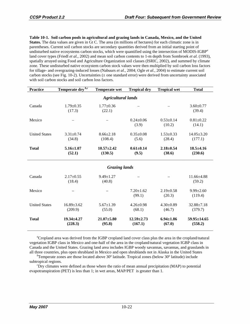
CCSP Product 2.2 Draft Four: Subsequent from Government Review
May 2007 10-22
Table 10-1. Soil carbon pools in agricultural and grazing lands in Canada, Mexico, and the United States. The data values are given in Gt C. The area (in millions of hectares) for each climatic zone is in parentheses. Current soil carbon stocks are secondary quantities derived from an initial starting point of undisturbed native ecosystems carbon stocks, which were quantified using the intersection of MODIS-IGBPa land cover types (Friedl et al., 2002) and mean soil carbon contents to 1-m depth from Sombroek et al. (1993), spatially arrayed using Food and Agriculture Organization soil classes (ISRIC, 2002), and summed by climate zone. These undisturbed native ecosystem carbon stock values were then multiplied by soil carbon loss factors for tillage- and overgrazing-induced losses (Nabuurs et al., 2004; Ogle et al., 2004) to estimate current soil carbon stocks (see Fig. 10-2). Uncertainties (± one standard error) were derived from uncertainty associated with soil carbon stocks and soil carbon loss factors. Practice Temperate dry b,c Temperate wet Tropical dry Tropical wet Total
Agricultural lands
Canada
1.79±0.35 (17.3)
1.77±0.36 (22.1)
–
–
3.60±0.77 (39.4)
Mexico
–
–
0.24±0.06 (3.9)
0.53±0.14 (10.2)
0.81±0.22 (14.1)
United States
3.31±0.74 (34.8)
8.66±2.18 (108.4)
0.35±0.08 (5.6)
1.53±0.33 (28.4)
14.05±3.20 (177.1)
Total
5.16±1.07 (52.1)
10.57±2.42 (130.5)
0.61±0.14 (9.5)
2.18±0.54 (38.6)
18.5±4.16 (230.6)
Grazing lands
Canada
2.17±0.55 (18.4)
9.49±1.27 (40.8)
–
–
11.66±4.88 (59.2)
Mexico
–
–
7.20±1.62 (99.1)
2.19±0.58 (20.3)
9.99±2.60 (119.4)
United States
16.89±3.62 (209.9)
5.67±1.39 (55.0)
4.26±0.98 (68.1)
4.30±0.89 (46.7)
32.88±7.18 (379.7)
Total
19.34±4.27 (228.3)
21.07±5.80 (95.8)
12.59±2.73 (167.1)
6.94±1.86 (67.0)
59.95±14.65 (558.2)
aCropland area was derived from the IGBP cropland land cover class plus the area in the cropland/natural vegetation IGBP class in Mexico and one-half of the area in the cropland/natural vegetation IGBP class in Canada and the United States. Grazing land area includes IGBP woody savannas, savannas, and grasslands in all three countries, plus open shrubland in Mexico and open shrublands not in Alaska in the United States
bTemperate zones are those located above 30º latitude. Tropical zones (below 30º latitude) include subtropical regions.
cDry climates were defined as those where the ratio of mean annual precipitation (MAP) to potential evapotranspiration (PET) is less than 1; in wet areas, MAP/PET is greater than 1.
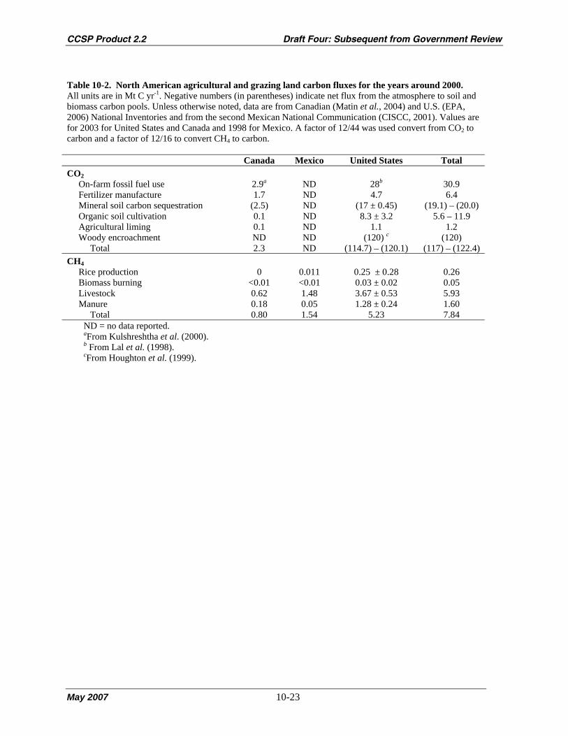
CCSP Product 2.2 Draft Four: Subsequent from Government Review
May 2007 10-23
Table 10-2. North American agricultural and grazing land carbon fluxes for the years around 2000. All units are in Mt C yr-1. Negative numbers (in parentheses) indicate net flux from the atmosphere to soil and biomass carbon pools. Unless otherwise noted, data are from Canadian (Matin et al., 2004) and U.S. (EPA, 2006) National Inventories and from the second Mexican National Communication (CISCC, 2001). Values are for 2003 for United States and Canada and 1998 for Mexico. A factor of 12/44 was used convert from CO2 to carbon and a factor of 12/16 to convert CH4 to carbon. Canada Mexico United States Total CO2 On-farm fossil fuel use 2.9a ND 28b 30.9 Fertilizer manufacture 1.7 ND 4.7 6.4 Mineral soil carbon sequestration (2.5) ND (17 ± 0.45) (19.1) – (20.0) Organic soil cultivation 0.1 ND 8.3 ± 3.2 5.6 – 11.9 Agricultural liming 0.1 ND 1.1 1.2 Woody encroachment ND ND (120) c (120) Total 2.3 ND (114.7) – (120.1) (117) – (122.4) CH4 Rice production 0 0.011 0.25 ± 0.28 0.26 Biomass burning <0.01 <0.01 0.03 ± 0.02 0.05 Livestock 0.62 1.48 3.67 ± 0.53 5.93 Manure 0.18 0.05 1.28 ± 0.24 1.60 Total 0.80 1.54 5.23 7.84
ND = no data reported. aFrom Kulshreshtha et al. (2000). b From Lal et al. (1998). cFrom Houghton et al. (1999).

CCSP Product 2.2 Draft Four: Subsequent from Government Review
May 2007 10-24
Fig. 10-1. North American agricultural and grazing land CO2 (left side) and methane (right side),
adjusted for global warming potential. All units are in Mt C-equivalent per year for years around 2000. Negative values indicate net flux from the atmosphere to soil and biomass carbon pools (i.e., sequestration). All data are from Canadian (Matin et al., 2004) and U.S. (EPA, 2006) National Inventories and from the second Mexican National Communication (CISCC, 2001), except for Canadian [from Kulshreshtha et al. (2000)] and U.S. fossil-fuel inputs [from Lal et al. (1998)] and woody encroachment [from Houghton et al. (1999)]. Values are for 2003 for Canada, 1998 for Mexico, and 2004 for the United States. A global warming potential of 23 for methane was used to convert emissions of CH4 to CO2 equivalents (IPCC, 2001) and a factor of 12/44 to convert from CO2 to carbon. Asterisks indicate unavailable data. Data ranges are indicated by error bars where available.
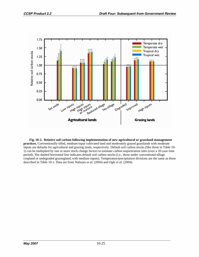
CCSP Product 2.2 Draft Four: Subsequent from Government Review
May 2007 10-25
Fig. 10-2. Relative soil carbon following implementation of new agricultural or grassland management practices. Conventionally tilled, medium-input cultivated land and moderately grazed grasslands with moderate inputs are defaults for agricultural and grazing lands, respectively. Default soil carbon stocks (like those in Table 10-1) can be multiplied by one or more stock change factors to estimate carbon sequestration rates (over a 20-year time period). The dashed horizontal line indicates default soil carbon stocks (i.e., those under conventional-tillage cropland or undegraded grazingland, with medium inputs). Temperature/precipitation divisions are the same as those described in Table 10-1. Data are from Nabuurs et al. (2004) and Ogle et al. (2004).

CCSP Product 2.2 Draft Four: Subsequent from Government Review
May 2007 10-26
[This page intentionally left blank]

CCSP Product 2.2 Draft Four: Subsequent from Government Review
May 2007 11-1
Chapter 11. North American Forests
Lead Authors: Richard A. Birdsey,1 Jennifer C. Jenkins,2 Mark Johnston3
and Elisabeth Huber-Sannwald4
Contributing Authors: Brian Amiro,5 Ben de Jong,6 Jorge D. Etchevers Barra,7 Nancy French,8
Felipe García Oliva,9 Mark Harmon,10 Linda S. Heath,1 Victor Jaramillo,9 Kurt Johnsen,1 Beverly E.
Law,10 Erika Marín-Spiotta,11 Omar Masera,9 Ronald Neilson,1 Yude Pan,1 and Kurt S. Pregitzer,12
1USDA Forest Service, 2University of Vermont, 3Saskatchewan Research Council, 4Instituto Potosino de
Investigación Científica y Tecnológica, 5University of Manitoba, 6ECOSUR, 7Colegio de Postgraduado,
8Altarum Institute, 9Universidad Nacional Autonoma de Mexico, 10Oregon State University, 11University of California at Berkeley, 12Michigan Technological University
KEY FINDINGS
• North American forests contain roughly 170 ± 40 billion tons of carbon, of which approximately 28% is
in live vegetation and 72% is in dead organic matter.
• North American forests were a net carbon sink of -270 ± 130 million tons of carbon per year over the
last 10 to 15 years.
• Deforestation continues in Mexico where forests are a source of carbon dioxide to the atmosphere.
Forests of the United States and parts of Canada have become a carbon sink as a consequence of
the recovery of forests following the abandonment of agricultural land.
• Carbon dioxide emissions from Canada’s forests are highly variable because of interannual changes
in area burned by wildfire.
• The size of the carbon sink in United States forests appears to be declining based on inventory data
from 1952 to the present.
• Many factors that cause changes in carbon stocks of forests have been identified, including land-use
change, timber harvesting, natural disturbance, increasing atmospheric carbon dioxide, climate
change, nitrogen deposition, and ozone in the lower atmosphere. There is a lack of consensus about
how these different natural and human-caused factors contribute to the current sink, and the relative
importance of factors varies geographically.
• There have been several continental- to subcontinental-scale assessments of future changes in
carbon and vegetation distribution in North America, but the resulting projections of future trends for
North American forests are highly uncertain. Some of this is due to uncertainty in future climate, but
there is also considerable uncertainty in forest response to climate change and in the interaction of
climate with other natural and human-caused factors.

CCSP Product 2.2 Draft Four: Subsequent from Government Review
May 2007 11-2
• Forest management strategies can be adapted to manipulate the carbon sink strength of forest
systems. The net effect of these management strategies will depend on the area of forests under
management, management objectives for resources other than carbon, and the type of disturbance
regime being considered.
• Decisions concerning carbon storage in North American forests and their management as carbon
sources and sinks will be significantly improved by (1) filling gaps in inventories of carbon pools and
fluxes, (2) a better understanding of how management practices affect carbon in forests, (3) better
estimate of potential changes in forest carbon under climate change and other factors, and (4) the
increased availability of decision support tools for carbon management in forests.
1. INTRODUCTION
The forest area of North America totals 771 million hectares, 36% of the land area of North America
and about 20% of the world’s forest area (Food and Agriculture Organization 2001) (see Table 11-1).†
About 45% of this forest area is classified as boreal, mostly in Canada and some in Alaska. Temperate
and tropical forests constitute the remainder of the forest area.
Table 11-1. Area of forest land by biome and country, 2000 (1000 ha).
North American forests are critical components of the global carbon cycle, exchanging large amounts
of carbon dioxide (CO2) and other gases with the atmosphere and oceans. In this chapter we present the
most recent estimates of the role of forests in the North American carbon balance, describe the main
factors that affect forest carbon stocks and fluxes, describe how forests the carbon cycle through CO2
sequestration and emissions, and discuss management options and research needs.
2. CARBON STOCKS AND FLUXES
2.1 Ecosystem Carbon Stocks and Pools
North American forests contain more than 170 billion tons of carbon (Gt C), of which 28% is in live
biomass and 72% is in dead organic matter (Table 11-2). Among the three countries, Canada’s forests
contain the most carbon and Mexico’s forests the least.
Table 11-2. Carbon stocks in forests by ecosystem carbon pool and country (Mt C).
† The uncertainties for all numerical values obtained from references to the tables in this chapter are explicitly provided in those tables.

CCSP Product 2.2 Draft Four: Subsequent from Government Review
May 2007 11-3
Carbon density (the amount of carbon stored per unit of land area) is highly variable. In Canada, the
majority of carbon storage occurs in boreal and cordilleran forests (Kurz and Apps, 1999). In the United
States, forests of the Northeast, Upper Midwest, Pacific Coast, and Alaska (with 14 Gt C) store the most
carbon. In Mexico, temperate forests contain 4.5 Gt C, tropical forests contain 4.1 Gt C, and semiarid
forests contain 5.0 Gt C.
2.2 Net North American Forest Carbon Fluxes
According to nearly all published studies, North American lands are a net carbon sink (Pacala et al.,
2001). A summary of currently available data from greenhouse gas inventories and other sources suggests
that the magnitude of the North American forest carbon sink was approximately -269 million tons of
carbon (Mt C) per year over the last decade or so, with United States forests accounting for most of the
sink (Table 11-3). This estimate is likely to be within 50% of the true value.
Table 11-3. Change in carbon stocks for forests and wood products by country (Mt C per year).
Canadian forests were estimated to be a net sink of -17 Mt C per year from 1990-2004 (Environment
Canada, 2005) (Table 11-3). These estimates pertain to the area of forest considered to be “managed”
under international reporting guidelines, which is 82% of the total area of Canada’s forests. The estimates
also include the carbon changes that result from land-use change. Changes in forest soil carbon are not
included. High interannual variability is averaged into this estimate—the annual change varied from
approximately -50 to +40 between 1990 and 2004. Years with net emissions were generally years with
high forest fire activity (Environment Canada, 2005) (Fig. 11-1).
Figure 11-1. Average and annual estimates of change in carbon stocks for forest ecosystems of
Canada, 1990-2004.
Most of the net sink in United States forests is in aboveground carbon pools, which account for -146
Mt C per year (Smith and Heath, 2005). The net sink for the belowground carbon pool is estimated at -90
Mt C (Pacala et al., 2001) (Table 11-3). The size of the carbon sink in United States forest ecosystems
appears to have declined slightly over the last decade (Smith and Heath, 2005). In contrast, a steady or
increasing supply of timber products now and in the foreseeable future (Haynes, 2003) means that the rate
of increase in the wood products carbon pool is likely to remain steady.

CCSP Product 2.2 Draft Four: Subsequent from Government Review
May 2007 11-4
For Mexico, the most comprehensive available estimate for the forest sector suggests a source of +52
Mt C per year in the 1990s (Masera et al., 1997) (Table 11-3). This estimate does not include changes in
the wood products carbon pool. The main cause of the estimated source is deforestation, which is offset to
a much lesser degree by restoration and recovery of degraded forestland.
Landscape-scale estimates of ecosystem carbon fluxes reflect the dynamics of individual forest stands
that respond to unique combinations of disturbance history, management intensity, vegetation, and site
characteristics. Extensive land-based measurements of forest/atmosphere carbon exchange for forest
stands at various stages of recovery after disturbance reveal patterns and causes of sink or source strength,
which is highly dependent on time since disturbance. Representative estimates for North America are
summarized in Appendix 11.A.
3. TRENDS AND DRIVERS
3.1 Overview of Trends and Drivers of Change in Carbon Stocks
Many factors that cause changes in carbon stocks of forests and wood products have been identified,
but the importance of each is still debated in the scientific literature (Barford et al., 2001; Caspersen et al.,
2000; Goodale et al., 2002; Korner, 2000; Schimel et al., 2000). Land-use change, timber harvesting,
natural disturbance, increasing atmospheric CO2, climate change, nitrogen deposition, and tropospheric
ozone all have effects on carbon stocks in forests, with their relative influence depending on geographic
location, the type of forest, and specific site factors. It is important for policy implementation and
management of forest carbon to separate the effects of direct human actions from natural factors.
The natural and human-caused (anthropogenic) factors that significantly influence forest carbon
stocks are different for each country, and still debated in the scientific literature. Natural disturbances are
significant in Canada, but estimates of the relative effects of different kinds of disturbance are uncertain.
One study estimated that impacts of wildfire and insects caused emissions of about +40 Mt C per year†† of
carbon to the atmosphere over the two decades (Kurz and Apps, 1999). Another study concluded that the
positive effects of climate, CO2, and nitrogen deposition outweighed the effects of wildfire and insects,
making Canada’s forests a net carbon sink in the same period (Chen et al., 2003). In the United States,
land use change and timber harvesting seem to be dominant factors according to repeated forest
inventories from 1952 to 1997 that show forest carbon stocks (excluding soils) increasing by about 175
Mt C per year. The most recent inventories show a decline in the rate of carbon uptake by forests, which
appears to be mainly the result of changing growth and harvest rates following a long history of land-use
change and management (Birdsey et al., 2006; Smith and Heath, 2005). The factors behind net emissions
†† The magnitude and/or range of uncertainty for the given numerical value(s) is not provided in the references cited.

CCSP Product 2.2 Draft Four: Subsequent from Government Review
May 2007 11-5
form Mexico’s forests are deforestation, forest degradation, and forest fires that are not fully offset by
forest regeneration (Masera et al., 1997; De Jong et al., 2000).
3.2 Effects of Land-Use Change
Since 1990, approximately 549,000 ha of former cropland or grassland in Canada have been
abandoned and are reverting to forest, while 71,000 ha of forest have been converted to cropland,
grassland, or settlements, for a net increase in forest area of 478,000 ha (Environment Canada, 2005).†† In
2004, approximately 25,000 ha were converted from forest to cropland, 19,000 ha from forest to
settlements and approximately 3,000 ha converted to wetlands. These land use changes resulted in
emissions of about 4 Mt C (Environment Canada 2005). ††
In the last century more than 130 million hectares of land in the conterminous United States were
either afforested (62 million ha) †† or deforested (70 million ha) †† (Birdsey and Lewis 2003). Houghton et
al. (1999) estimated that cumulative changes in forest carbon stocks for the period from 1700 to 1990 in
the United States were about +25 Gt C, †† primarily from conversion of forestland to agricultural use and
reduction of carbon stocks for wood products.
Emissions from Mexican forests to the atmosphere are primarily due to the impacts of deforestation to
pasture and degradation of 720,000 to 880,000 ha per year†† (Masera et al., 1997; Palacio et al. 2000).
The highest deforestation rates occur in the tropical deciduous forests (304,000 ha in 1990) †† and the
lowest in temperate broadleaf forests (59,000 ha in 1990). ††
3.3 Effects of Forest Management
The direct human impact on North American forests ranges from very minimal for protected areas to
very intense for plantations (Table 11-4). Between these extremes is the vast majority of forestland, which
is impacted by a wide range of human activities and government policies that influence harvesting, wood
products, and regeneration.
Table 11-4. Area of forestland by management class and country, 2000 (1000 ha).
Forests and other wooded land in Canada occupy about 402 million ha. Approximately 310 million ha
is considered forest of which 255 million ha (83%) are under active forest management (Environment
Canada, 2005). †† Managed forests are considered to be under the direct influence of human activity and
not reserved. Less than 1% of the area under active management is harvested annually. Apps et al. (1999)
used a carbon budget model to simulate carbon in harvested wood products (HWP) for Canada.
Approximately 800 Mt C were stored in the Canadian HWP sector in 1989, of which 50 Mt C were in

CCSP Product 2.2 Draft Four: Subsequent from Government Review
May 2007 11-6
imported wood products, 550 Mt C in exported products, and 200 Mt C in wood products produced and
consumed domestically. ††
Between 1990 and 2000, about 4 million ha per year were harvested in the United States, two-thirds
by partial-cut harvest and one-third by clear-cut (Birdsey and Lewis, 2003). Between 1987 and 1997,
about 1 million ha per year were planted with trees, and about 800,000 ha were treated to improve the
quality and/or quantity of timber produced (Birdsey and Lewis, 2003). Harvesting in United States forests
accounts for substantially more tree mortality than natural causes such as wildfire and insect outbreaks
(Smith et al., 2004). The harvested wood resulted in -57 Mt C added to landfills and products in use, and
an additional 88 Mt C were emitted from harvested wood burned for energy (Skog and Nicholson,
1998).††
About 80% of the forested area in Mexico is socially owned by communal land grants (ejidos) and
rural communities. About 95% of timber harvesting occurs in native temperate forests (SEMARNAP,
1996). Illegal harvesting involves 13.3 million m3 of wood every year (Torres, 2004). The rural
population is the controlling factor for changes in carbon stocks from wildfire, wood extraction, shifting
agriculture practices, and conversion of land to crop and pasture use.
3.4 Effects of Climate and Atmospheric Chemistry
Environmental factors, including climate variability, nitrogen deposition, tropospheric ozone, and
elevated CO2, have been recognized as significant factors affecting the carbon cycle of forests (Aber et
al., 2001; Ollinger et al., 2002). Some studies indicate that these effects are significantly smaller than the
effects of land management and land-use change (Caspersen et al., 2000; Schimel et al., 2000). Recent
reviews of ecosystem-scale studies known as Free Air CO2 Exchange (FACE) experiments suggest that
rising CO2 increases net primary productivity by 12-23% over all species studied (Norby et al., 2005;
Nowak et al., 2004). However, it is uncertain whether this effect results in a lasting increase in
sequestered carbon or causes a more rapid cycling of carbon between the ecosystem and the atmosphere
(Korner et al., 2005; Lichter et al., 2005). Experiments have also shown that the effects of rising CO2 are
significantly moderated by increasing tropospheric ozone (Karnosky et al., 2003; Loya et al., 2003).
When nitrogen availability is also considered, reduced soil fertility limits the response to rising CO2, but
nitrogen deposition can increase soil fertility to counteract that effect (Finzi et al. 2006; Johnson et al.,
1998; Oren et al., 2001). Observations of photosynthetic activity from satellites suggest that productivity
changes due to lengthening of the growing season depend on whether areas were disturbed by fire (Goetz
et al., 2005). Based on these conflicting and complicated results from different studies and approaches, a
definitive assessment of the relative importance, and interactions, of natural and anthropogenic factors is a
high priority for research (U.S. Climate Change Science Program, 2003).

CCSP Product 2.2 Draft Four: Subsequent from Government Review
May 2007 11-7
3.5 Effects of Natural Disturbances
Wildfire, insects, diseases, and weather events are common natural disturbances in North America.
These factors impact all forests but differ in magnitude by geographic region.
Wildfires were the largest disturbance in the twentieth century in Canada (Weber and Flannigan,
1997). In the 1980s and 1990s, the average total burned area was 2.6 million ha per year in Canada’s
forests, with a maximum 7.6 million ha per year in 1989. †† Carbon emissions from forest fires range from
less than +1 Mt C per year in the interior of British Columbia to more than +10 Mt C per year in the
western boreal forest. Total emissions from forest fires in Canada averaged approximately +27 Mt C per
year between 1959 and 1999 (Amiro et al., 2001). †† Estimated carbon emissions from four major insect
pests in Canadian forests (spruce budworm, jack pine budworm, hemlock looper, and mountain pine
beetle) varied from +5 to 10 Mt C per year in the 1970s to less than +2 Mt C per year in the mid-1990s1.
Much of the Canadian forest is expected to experience increases in fire severity (Parisien et al., 2005) and
burn areas (Flannigan et al., 2005), and continued outbreaks of forest pests are also likely (Volney and
Hirsch, 2005).
In United States forests insects, diseases, and wildfire combined affect more than 30 million ha per
decade (Birdsey and Lewis, 2003). Damage from weather events (hurricanes, tornados, and ice storms)
may exceed 20 million ha per decade (Dale et al., 2001). Although forest inventory data reveal the extent
of tree mortality attributed to all causes combined, estimates of the impacts of individual categories of
natural disturbance on carbon pools of temperate forests are scarce. The impacts of fire are clearly
significant. According to one estimate, the average annual carbon emissions from biomass burning in the
contemporary United States ranges from 9 to 59 Mt C (Leenhouts, 1998). McNulty (2002) estimated that
large hurricanes in the United States could convert 20 Mt C of live biomass into detrital carbon pools.
The number and area of sites affected by forest fires in Mexico have fluctuated considerably between
1970 and 2002 with a clear tendency of an increasing number of fire events (4,000-7,000 in the 1970s and
1,800-15,000 in the 1990s), and overall, larger areas are being affected (0.08-0.25 million ha in 1970s and
0.05-0.85 million ha in 1990s). During El Nino years, increasing drought increases fire frequencies
(Torres, 2004). Between 1995 and 2000, an average 8,900 fire events occurred per year and affected
about 327,000 ha of the forested area. Currently, no estimates are available on the contribution of these
fires to CO2 emissions. Pests and diseases are important natural disturbance agents in temperate forests of
Mexico; however, no statistics exist on the extent of the affected land area.
1These estimates are the product of regional carbon density values, the proportion of mortality in defoliated stands given in
Kurz and Apps (1999), data on area affected taken from NFDP (2005), and the proportion of C in insect-killed stands that is emitted directly to the atmosphere (0.1) from the disturbance matrix for insects used in the CBM-CFS (Kurz et al., 1992).
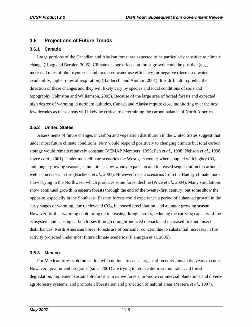
CCSP Product 2.2 Draft Four: Subsequent from Government Review
May 2007 11-8
3.6 Projections of Future Trends
3.6.1 Canada
Large portions of the Canadian and Alaskan forest are expected to be particularly sensitive to climate
change (Hogg and Bernier, 2005). Climate change effects on forest growth could be positive (e.g.,
increased rates of photosynthesis and increased water use efficiency) or negative (decreased water
availability, higher rates of respiration) (Baldocchi and Amthor, 2001). It is difficult to predict the
direction of these changes and they will likely vary by species and local conditions of soils and
topography (Johnston and Williamson, 2005). Because of the large area of boreal forests and expected
high degree of warming in northern latitudes, Canada and Alaska require close monitoring over the next
few decades as these areas will likely be critical to determining the carbon balance of North America.
3.6.2 United States Assessments of future changes in carbon and vegetation distribution in the United States suggest that
under most future climate conditions, NPP would respond positively to changing climate but total carbon
storage would remain relatively constant (VEMAP Members, 1995; Pan et al., 1998; Neilson et al., 1998;
Joyce et al., 2001). Under most climate scenarios the West gets wetter; when coupled with higher CO2
and longer growing seasons, simulations show woody expansion and increased sequestration of carbon as
well as increases in fire (Bachelet et al., 2001). However, recent scenarios from the Hadley climate model
show drying in the Northwest, which produces some forest decline (Price et al., 2004). Many simulations
show continued growth in eastern forests through the end of the twenty-first century, but some show the
opposite, especially in the Southeast. Eastern forests could experience a period of enhanced growth in the
early stages of warming, due to elevated CO2, increased precipitation, and a longer growing season.
However, further warming could bring on increasing drought stress, reducing the carrying capacity of the
ecosystem and causing carbon losses through drought-induced dieback and increased fire and insect
disturbances. North American boreal forests are of particular concern due to substantial increases in fire
activity projected under most future climate scenarios (Flannigan et al. 2005).
3.6.3 Mexico
For Mexican forests, deforestation will continue to cause large carbon emissions in the years to come.
However, government programs (since 2001) are trying to reduce deforestation rates and forest
degradation, implement sustainable forestry in native forests, promote commercial plantations and diverse
agroforestry systems, and promote afforestation and protection of natural areas (Masera et al., 1997).

CCSP Product 2.2 Draft Four: Subsequent from Government Review
May 2007 11-9
4. OPTIONS FOR MANAGEMENT
Forest management strategies can be adapted to increase the amount of carbon uptake by forest
systems. Alternative strategies for wood products are also important in several ways: how long carbon is
retained in use, how much wood is used for biofuel, and substitution of wood for other materials that use
more energy to produce. The net effect of these management and production strategies on carbon stocks
and emissions will depend on emerging government policies for greenhouse gas management, the area of
forests under management, management objectives for resources other than carbon, and the type of
management and production regime being considered.
The forest sector includes a variety of activities that can contribute to increasing carbon sequestration,
including: afforestation, mine land reclamation, forest restoration, agroforestry, forest management,
biomass energy, forest preservation, wood products management, and urban forestry (Birdsey et al.,
2000). Although the science of managing forests specifically for carbon sequestration is not well
developed, some ecological principles are emerging to guide management decisions (Appendix 11.B).
The prospective role of forestry in helping to stabilize atmospheric CO2 depends on government policy,
harvesting and disturbance rates, expectations of future forest productivity, the fate and longevity of forest
products, and the ability to deploy technology and forest practices to increase the retention of sequestered
CO2. Market factors are also important in guiding the behavior of the private sector.
For Canada, Price et al. (1997) examined the effects of reducing natural disturbance, manipulating
stand density, and changing rotation lengths for a forested landscape in northwest Alberta. By replacing
natural disturbance (fire) with a simulated harvesting regime, they found that long-term equilibrium
carbon storage increased from 105 to 130 Mt C. Controlling stand density following harvest had minimal
impacts in the short term but increased landscape-level carbon storage by 13% after 150 years. Kurz et al.
(1998) investigated the impacts on landscape-level carbon storage of the transition from natural to
managed disturbance regimes. For a boreal landscape in northern Quebec, a simulated fire disturbance
interval of 120 yr was replaced by a harvest cycle of 120 yr. The net impact was that the average age of
forests in the landscape declined from 110 yr to 70 yr, and total carbon storage in forests declined from
16.3 to 14.8 Mt C (including both ecosystem and forest products pools).
Market approaches and incentive programs to manage greenhouse gases, particularly CO2, are under
development in the United States, the European Union, and elsewhere (Totten, 1999). Since forestry
activities have highly variable costs because of site productivity and operational variability, most recent
studies of forestry potential develop “cost curves”, i.e., estimates of how much carbon will be sequestered
by a given activity for various carbon prices (value in a market system) or payments (in an incentive
system). There is also a temporal dimension to the analyses because the rate of change in forest carbon

CCSP Product 2.2 Draft Four: Subsequent from Government Review
May 2007 11-10
stocks is variable over time, with forestry activities tending to have a high initial rate of net carbon
sequestration followed by a lower or even a negative rate as forests reach advanced age.
In the United States, a bundle of forestry activities could potentially increase carbon sequestration
from -100 to -200 Mt C per year according to several studies (Birdsey et al., 2000; Lewandrowski et al.,
2004; Environmental Protection Agency, 2005; Stavins and Richards, 2005). The rate of annual
mitigation would likely decline over time as low-cost forestry opportunities become scarcer, forestry
sinks become saturated, and timber harvesting takes place. Economic analyses of the U.S. forestry
potential have focused on three broad categories of activities: afforestation (conversion of agricultural
land to forest), improved management of existing forests, and use of woody biomass for fuel. Improved
management of existing forest lands may be attractive to landowners at a carbon prices below $10 per ton
of CO2; afforestation requires a moderate price of $15 per ton of CO2 or more to induce landowners to
participate; and biofuels become dominant at prices of $30-50 per ton of CO2 (Lewandrowski et al., 2004;
Stavins and Richards, 2005; Environmental Protection Agency, 2005). Table 11-5 shows a simple
scenario of emissions reduction below baseline, annualized over the time period 2010-2110, for forestry
activities as part of a bundle of reduction options for the land base.
Table 11-5. Illustrative emissions reduction potential of various forestry activities in the United
States under a range of prices and sequestration rates.
Production of renewable materials that have lower life-cycle emissions of greenhouse gases than non-
renewable alternatives is a promising strategy for reducing emissions. Lippke et al. (2004) found that
wood components used in residential construction had lower emissions of CO2 from energy inputs than
either concrete or steel.
Co-benefits are vitally important for inducing good forest carbon management. For example,
conversion of agricultural land to forest will generally have positive effects on water, air, and soil quality
and on biodiversity. In practice, some forest carbon sequestration projects have already been initiated
even though sequestered carbon has little current value (Winrock International, 2005). In many of the
current projects, carbon is a secondary objective that supports other landowner interests, such as
restoration of degraded habitat. But co-effects may not all be beneficial. Water quantity may decline
because of increased transpiration by trees relative to other vegetation. And taking land out of crop
production may affect food prices—at higher carbon prices, nearly 40 million ha may be converted from
cropland to forest (Environmental Protection Agency, 2005). Implementation of a forest carbon
management policy will need to carefully consider co-effects, both positive and negative.
CCSP Product 2.2 Draft Four: Subsequent from Government Review
May 2007 11-11
5. DATA GAPS AND INFORMATION NEEDS FOR DECISION SUPPORT
Decisions concerning carbon storage in North American forests and their management as carbon
sources and sinks will be significantly improved by (1) filling gaps in inventories of carbon pools and
fluxes, (2) a better understanding of how management practices affect carbon in forests, and (3) the
increased availability of decision support tools for carbon management in forests.
5.1 Major Data Gaps in Estimates of Carbon Pools and Fluxes
Effective carbon policy and management to increase carbon sequestration and/or reduce emissions
requires thorough understanding of current carbon stock sizes and flux rates, and responses to
disturbance. Data gaps complicate analyses of the potential for policies to influence natural, social and
economic drivers that can change carbon stocks and fluxes. Forests in an area as large as North America
are quite diverse, and comprehensive data sets that can be used to analyze forestry opportunities, such as
spatially explicit historical management and disturbance rates and effects on the carbon cycle, would
enable managers to change forest carbon stocks and fluxes. Although this report provides aggregate
statistics on forest carbon by biome and country, users could benefit from spatially explicit estimates of
forest carbon. Such an analysis might involve matching estimates based on forest inventories as presented
by political unit and general forest type (Birdsey and Lewis, 2003) with data developed using remote
sensing techniques (Running et al., 2004). Research at the level of individual sites has proven the
feasibility of this combination (e.g., Van Tuyl et al., 2005; Turner et al., 2006). This kind of analysis
could facilitate development of a forest carbon map for North America.
In the United States, the range of estimates of the size of the land carbon sink is between 0.30 and
0.58 Mt C per year (Pacala et al., 2001). Significant data gaps among carbon pools include carbon in
wood products, soils, woody debris, and water transport (Birdsey, 2004; Pacala et al., 2001). Geographic
areas that are poorly represented in the available data sets include much of the Intermountain Western
United States and Alaska, where forests of low productivity have not been inventoried as intensively as
more productive timberlands (Birdsey, 2004). Accurate quantification of the relative magnitude of various
causal mechanisms at large spatial scales is not yet possible, although research is ongoing to combine
various approaches and data sets: large-scale observations, process-based modeling, ecosystem
experiments, and laboratory investigations (Foley and Ramankutty, 2004).
Data gaps exist for Canada, particularly regarding changes in forest soil carbon and forestlands that
are considered “unmanaged” (17% of forest lands). Aboveground biomass is better represented in forest
inventories; however, the information needs to be updated and made more consistent among provinces.
The new Canadian National Forest Inventory, currently under way, will provide a uniform coverage at a
20 × 20 km grid that will be the basis for future forest carbon inventories. Data are also lacking on carbon

CCSP Product 2.2 Draft Four: Subsequent from Government Review
May 2007 11-12
fluxes, particularly those due to insect outbreaks and forest stand senescence. The ability to model forest
carbon stock changes has considerably improved with the release of the Carbon Budget Model of the
Canadian Forest Sector (CBM-CFS3)(Kurz et al., 2002); however, the CBM-CFS3 was not designed to
incorporate climate change impacts (Price et al., 1999; Hogg and Bernier, 2005).
For Mexico, there is very little data about measured carbon stocks for all forest types. Information on
forest ecosystem carbon fluxes is primarily based on deforestation rates, while fundamental knowledge of
carbon exchange processes in almost all forest ecosystems is missing. That information is essential for
understanding the effects of both natural and human-induced drivers (hurricanes, fires, insect outbreaks,
climate change, migration, and forest management strategies), which all strongly impact the forest carbon
cycle. Current carbon estimates are derived from studies in preferred sites in natural reserves with
species-rich tropical forests. Therefore, inferences made from the studies on regional and national carbon
stocks and fluxes probably give biased estimates on the carbon cycle.
5.2 Major Data Gaps in Knowledge of Forest Management Effects
There is insufficient information available to guide land managers in specific situations to change
forest management practices to increase carbon sequestration, and there is some uncertainty about the
longevity of effects (Caldeira et al., 2004). This reflects a gap in the availability of inexpensive
techniques for measuring, monitoring, and predicting changes in ecosystem carbon pools at the smaller
scales appropriate for managers. There is more information available about management effects on live
biomass and woody debris, and less about effects on soils and wood products. This imbalance in data has
the potential to produce unintended consequences if predicted results are based on incomplete carbon
accounting.
In the tropics, agroforestry systems offer a promising economic alternative to slash-and-burn
agriculture, including highly effective soil conservation practices and mid-term and long-term carbon
mitigation options (Soto-Pinto et al., 2001; Nelson and de Jong, 2003; Albrecht and Kandji, 2003).
However, a detailed assessment of current implementations of agroforestry systems in different regions of
Mexico is missing. Agroforestry also has potential in temperate agricultural landscapes, but as with forest
management, there is a lack of data about how specific systems affect carbon storage (Nair and Nair,
2003).
Refining management of forests to realize significant carbon sequestration while at the same time
continuing to satisfy the other needs and services of provided by forests (e.g., timber harvest, recreational
value, watershed management) will require a multi-criteria decision support framework for a holistic and
adaptive management program of the carbon cycle in North American forests. For example, methods
should be developed for enhancing the efficiency of forest utilization as a renewable energy source,

CCSP Product 2.2 Draft Four: Subsequent from Government Review
May 2007 11-13
increasing the carbon storage per acre from existing forests, or even increasing the acreage devoted to
forest systems that provide carbon sequestration. Currently there is little information about how
appropriate incentives might be applied to accomplish these goals effectively, but given the importance of
forests in the global carbon cycle, success in this endeavor could have important long-term and large-
scale effects on global atmospheric carbon stocks.
5.3 Availability Of Decision-Support Tools
Few decision-support tools for land managers that include complete carbon accounting are available;
one example is the CBM-CFS3 carbon accounting model (Kurz et al., 2002). Some are in development or
have been used primarily in research studies (Proctor et al., 2005; Potter et al., 2003). As markets emerge
for trading carbon credits, and if credits for forest management activities have value in those markets,
then the demand for decision-support tools will encourage their development.
CHAPTER 11 REFERENCES
Aber, J., R.P. Neilson, S. McNulty, J.M. Lenihan, D. Bachelet, and R.J. Drapek, 2001: Forest processes and global
change: predicting the effects of individual and multiple stressors. BioScience 51(9), 735-751.
Albrecht, A. and S.T. Kandji, 2003: Carbon sequestration in tropical agroforestry systems. Agriculture, Ecosystems
and Environments, 99, 15-27.
Amiro, B.D., J.B. Todd, B.M. Wotton, K.A. Logan, M.D. Flannigan, B.J. Stocks, J.A. Mason, D.L. Martell and
K.G. Hirsch, 2001: Direct carbon emissions from Canadian forest fires, 1959-1999. Canadian Journal of Forest
Research, 31, 512-525.
Apps, M.J., W.A. Kurz, S.J. Beukema, and J.S. Bhatti, 1999: Carbon budget of the Canadian forest product sector.
Environmental Science & Policy, 2, 25-41.
Bachelet, D., R.P. Neilson, J.M. Lenihan, and R.J. Drapek, 2001: Climate change effects on vegetation distribution
and carbon budget in the United States. Ecosystems, 4, 164-185.
Baldocchi, D.D. and J.S. Amthor, 2001: Canopy photosynthesis: history, measurements and models. In: Terrestrial
Global Productivity [Roy, J., B. Saugier, and H. Mooney (eds.)]. Academic Press, San Diego, USA, pp. 9-31.
Barford C.C., S.C. Wofsy, M.L. Goulden, J.W. Munger, E.H. Pyle, S.P. Urbanski, L. Hutyra, S.R. Saleska, D.
Fitzjarrald, and K. Moore, 2001: Factors controlling long- and short-term sequestration of atmospheric CO2 in a
mid-latitude forest. Science, 294, 1688-1691.
Bechtold, W.A. and P.L. Patterson (eds.), 2005: The Enhanced Forest Inventory and Analysis Program - National
Sampling Design and Estimation Procedures. General Technical Report SRS-80, U.S. Department of
Agriculture, Forest Service, Southern Research Station, Asheville, NC, 85 pp.
Birdsey, R.A. and L.S. Heath, 1995: Carbon changes in U.S. forests. In: Climate Change and the Productivity Of
America's Forests [Joyce, L.A. (ed.)]. U. S. Department of Agriculture, Forest Service, Rocky Mountain Forest
and Range Experiment Station General Technical Report, Fort Collins, CO, pp. 56-70.
CCSP Product 2.2 Draft Four: Subsequent from Government Review
May 2007 11-14
Birdsey, R.A., R. Alig, and D. Adams, 2000: Migitation activities in the forest sector to reduce emissions and
enhance sinks of greenhouse gases. In: The Impact of Climate Change on America's Forests: A Technical
Document Supporting the 2000 USDA Forest Service RPA Assessment [Joyce, L.A. and R.A. Birdsey (eds.]).
RMRS-GTR-59, U.S. Department of Agriculture, Forest Service, Rocky Mountain Research Station, Fort
Collins, CO, pp. 112-131.
Birdsey, R.A., 2004: Data gaps for monitoring forest carbon in the United States: an inventory perspective. In:
[Mickler, R.A. (ed.)]. Environmental Management, 33(Suppl. 1), S1-S8.
Birdsey, R.A. and G.M. Lewis, 2003: Current and historical trends in use, management, and disturbance of U.S.
forestlands. In: The Potential of U.S. Forest Soils to Sequester Carbon and Mitigate the Greenhouse Effect
[Kimble, J.M., L.S. Heath, and R.A. Birdsey (eds.)]. CRC Press LLC, New York, NY, pp. 15-33.
Birdsey, R., K. Pregitzer, and A. Lucier, 2006: Forest carbon management in the United States, 1600-2100. Journal
of Environmental Quality (in press).
Caldeira, K., M.G. Morgan, D. Baldocchi, P.G. Brewer, C.-T.A. Chen, G.-J. Nabuurs, N. Nakicenovic, and G.P.
Robertson, 2004: A portfolio of carbon management options. In: The Global Carbon Cycle [Field, C.B. and
M.R. Raupach (eds.)]. Island Press. Washington, DC.
Canadian Forest Service, 2005: State of the Forest Report, 2004-2005. Canadian Forest Service, Natural
Resources Canada, Ottawa, Ontario, Canada. Available at http://www.nrcan-rncan.gc.ca/cfs-scf/national/what-
quoi/sof/latest_e.html
Caspersen, J.P., S.W. Pacala, J.C. Jenkins, G.C. Hurtt, P.R. Moorcraft, and R.A. Birdsey, 2000: Contributions of
land-use history to carbon accumulation in U.S. forests. Science, 290, 1148-1151.
Chen, J.M., W. Ju, and J. Cihlar, et al., 2003: Spatial distribution of carbon sources and sinks in Canada’s forests.
Tellus B, 1-20.
Dale, V.H., L.A. Joyce, S. McNulty, R.P. Neilson, et al., 2001: Climate change and forest disturbances. Bioscience,
51(9), 723-734.
De Jong, B.H.J., S. Ochoa-Gaona, M.A. Castillo-Santiago, N. Ramirez-Marcial, and M.A. Cairns, 2000: Carbon
fluxes and patterns of land-use/land-cover change in the Selva Lacandona, Mexico. Ambio, 29, 504-511.
Environment Canada, 2005: Canada’s Greenhouse Gas Inventory 1990-2004: Initial Submission. Greenhouse Gas
Division, Environment Canada, Ottawa, Ontario, Canada. Available at
http://unfccc.int/national_reports/annex_i_ghg_inventories/national_inventories_submissions/items/2761.php
Environmental Protection Agency, 2005: Greenhouse Gas Mitigation Potential in U.S. Forestry and Agriculture.
U.S. Environmental Protection Agency, Washington, DC, 154 pp.
Finzi, A.C., D.J.P. Moore, E.H. DeLucia, J. Lichter, K.S. Hofmockel, R.P. Jackson, H.-S. Kim, R. Matamala, H.R.
McCarthy, R. Oren, J.S. Pippen, and W.H. Schlesinger, 2006: Progressive nitrogen limitation of ecosystem
processes under elevated CO2 in a warm-temperate forest. Ecology, 87(1), 15-25.
Flannigan, M.D., K.A. Logan, B.D. Amiro, W.R. Skinner, and B.J. Stocks, 2005: Future area burned in Canada.
Climatic Change, 72, 1-16.

CCSP Product 2.2 Draft Four: Subsequent from Government Review
May 2007 11-15
Foley, J.A. and N. Ramankutty, 2004: A primer on the terrestrial carbon cycle: what we don’t know but should. In:
The Global Carbon Cycle [Field, C.B. and M.R. Raupach (eds.)]. Island Press, Washington, DC.
Food and Agriculture Organization, 2001: Global Forest Resources Assessment 2000. Main Report. FAO
Forestry Paper 140, Rome, Italy, 481 pp.
Goetz, S.J., A.G. Bunn, G.J. Fiske, and R.A. Houghton, 2005: Satellite-observed photosynthetic trends across boreal
North America associated with climate and fire disturbance. PNAS, 102(38), 13521-13525.
Goodale, C.L., M.J. Apps, R.A. Birdsey, C.B. Field, L.S. Heath, R.A. Houghton, J.C. Jenkins, G.H. Kohlmaier, W.
Kurz, S. Liu, G.-J. Nabuurs, S. Nilsson, and A.Z. Shvidenko, 2002: Forest carbon sinks in the northern
hemisphere. Ecological Applications, 12, 891-899.
Haynes, R.W. (ed.), 2003: An Analysis of the Timber Situation in the United States: 1952-2050. General Technical
Report PNW-GTR-560, USDA Forest Service, Portland, OR, 254 pp.
Heath, L.S. and J.E. Smith, 2004: Criterion 5, indicator 26: total forest ecosystem biomass and carbon pool, and if
appropriate, by forest type, age class and successional change. In: Data Report: A Supplement to the National
Report on Sustainable Forests—2003 [Darr, D.R. (coord.)]. FS-766A, U.S. Department of Agriculture,
Washington, DC, 14 pp. Available at http://www.fs.fed.us/research/sustain/contents.htm (8 June).
Heath, L.S. and J. E. Smith, 2000: An assessment of uncertainty in forest carbon budget projections. Environmental
Science & Policy, 3, 73-82.
Hogg, E.H. and P.Y. Bernier, 2005: Climate change impacts on drought-prone forests in western Canada. Forestry
Chronicle (in press).
Houghton, R.A., J.L. Hackler, and K.T. Lawrence, 1999: The U.S. carbon budget: contributions from land-use
change, Science, 285, 574-578.
Johnson, D.W., R.B. Thomas, K.L. Griffen, and D.T. Tissue, et al., 1998: Effects of carbon dioxide and nitrogen on
growth and nitrogen uptake in ponderosa and loblolly pine. Journal of Environmental Quality, 27, 414-425.
Johnston, M. and T. Williamson, 2005: Climate change implications for stand yields and soil expectation values: a
northern Saskatchewan case study. Forestry Chronicle, 81, 683-690.
Joyce, L., J. Baer, S. McNulty, V. Dale, A. Hansen, L. Irland, R. Neilson, and K. Skog, 2001: Potential
consequences of climate variability and change for the forests of the United States: In: Climate Change Impacts
in the United States. Report for the U.S Global Change Research Program. Cambridge University Press,
Cambridge, UK, pp. 489-521.
Karnosky, D.F., D.R. Zak, K.S. Pregitzer, C.S. Awmack, et al., 2003: Tropospheric ozone moderates responses of
temperate hardwood forests to elevated CO2: a synthesis of molecular to ecosystem results from the Aspen
FACE project. Functional Ecology, 17, 289-304.
Korner, C., 2000: Biosphere responses to CO2 enrichment. Ecological Applications, 10, 1590-1619.
Korner, C., R. Asshof, O. Bignucolo, and S. Haattenschwiler, et al., 2005. Carbon flux and growth in mature
decidous forest trees exposed to elevated CO2. Science, 309, 1360-1362.
CCSP Product 2.2 Draft Four: Subsequent from Government Review
May 2007 11-16
Kurz, W.A., M.J. Apps, T.M. Webb, and P.J. McNamee, 1992: The Carbon Budget of the Canadian Forest Sector:
Phase 1. Information Report NOR-X-326, Forestry Canada, Northern Forestry Centre, Edmonton, Alberta,
Canada.
Kurz, W.A., S. Beukema, and M.J. Apps: 1998: Carbon budget implications of the transition from natural to
managed disturbance regimes in forest landscapes. Mitigation and Adaptation Strategies for Global Change, 2,
405-421.
Kurz, W.A. and M.J. Apps, 1999: A 70-year retrospective analysis of carbon fluxes in the Canadian forest sector.
Ecological Applications, 9, 526-547.
Kurz, W., M. Apps, E. Banfield, and G. Stinson, 2002: Forest carbon accounting at the operational scale. The
Forestry Chronicle, 78, 672-679.
Leenhouts, B., 1998: Assessment of biomass burning in the conterminous United States. Conservation Ecology,
2(1), 1.
Lewandrowski, J., M. Sperow, M. Peters, M. Eve, C. Jones, K. Paustian, and R. House, 2004: Economics of
Sequestering Carbon in the U.S. Agricultural Sector. Technical Bulletin 1909, U.S. Department of Agriculture,
Economic Research Service, Washington, DC, 61 pp.
Lichter, J., S.H. Barron, C.E. Bevacqua, A.C. Finzi, K.F. Irvine, et al., 2005: Soil carbon sequestration and turnover
in a pine forest after six years of atmospheric CO2 enrichment. Ecology, 86(7), 1835-1847.
Lippke, B., J. Wilson, J. Perez-Garcia, J. Bowyer, and J. Miel, 2004: CORRIM: Life cycle environmental
performance of renewable building materials. Forest Products Journal, 54(6), 8-19.
Loya, W.M., K.S. Pregitzer, N.J. Karberg, J.S. King, and C.P. Giardina, 2003: Reduction of soil carbon formation
by tropospheric ozone under increased carbon dioxide levels. Nature, 425, 705-707.
Masera, O., M.J. Ordóñez, and R. Dirzo, 1997: Carbon emissions from Mexican forests: the current situation and
long-term scenarios. Climatic Change, 35, 265-295.
Masera, O., A. Delia Cerón, and A. Ordóñez, 2001: Forestry mitigation options for Mexico: finding synergies
between national sustainable development priorities and global concerns. Mitigation and Adaptation Strategies
for Global Change, 6, 291-312.
McNulty, S.G., 2002: Hurricane impacts on U.S. forest carbon sequestration. Environmental Pollution, 116, S17-
S24.
Nair, P.K.R, and V.D. Nair, 2003: Carbon storage in North American agroforestry systems. In: Kimble, J., L.S.
Heath, R.A. Birdsey, and R. Lal (eds.). The Potential of U.S. Forest Soils to Sequester Carbon and Mitigate the
Greenhouse Gas Effect. CRC Press, Boca Raton, FL, pp. 333-346.
Natural Resources Canada, 2005: The State of Canada's Forests. Canadian Forest Service, Natural Resources
Canada, Ottawa, Ontario, Canada. Available at http://www.nrcan-rncan.gc.ca/cfs-scf/national/what-
quoi/sof/latest_e.html
Neilson, R.P., I.C. Prentice, B. Smith, T.G.F. Kittel, and D. Viner, 1998: Simulated changes in vegetation
distribution under global warming. In: The Regional Impacts of Climate Change: An Assessment of
CCSP Product 2.2 Draft Four: Subsequent from Government Review
May 2007 11-17
Vulnerability [Watson, R.T., M.C. Zinyowera, R.H. Moss, and D.J. Dokken (eds.)]. Cambridge University
Press, Cambridge, UK, pp. 439-456.
Nelson, K.C. and B.H.J. de Jong, 2003: Making global initiatives local realities: carbon mitigation projects in
Chiapas, Mexico. Global Environmental Change, 13, 19-30.
NFDP (National Forestry Database Program), 2005: Compendium of Canadian Forestry Statistics. National
Forestry Database Program, Canadian Council of Forest Ministers, Ottawa, Ontario, Canada. Available at
http://nfdp.ccfm.org/compendium/index_e.php
Norby, R.J., E.H. DeLucia, and B. Gielen, et al., 2005: Forest response to elevated CO2 is conserved across a broad
range of productivity. Proceedings of the National Academy of Sciences of the United States of America,
102(50), 18052-18056.
Nowak, R.S., D.S. Ellsworth, and S.D. Smith, 2004: Functional responses of plants to elevated atmospheric CO2- do
photosynthetic and productivity data from FACE experiments support early predictions? New Phytologist,
162(2), 253.
Ollinger S.V, J.D. Aber, P.B. Reich, and R.J. Freuder, 2002: Interactive effects of nitrogen deposition, tropospheric
ozone, elevated CO2 land use history on the carbon dynamics of northern hardwood forests. Global Change
Biology, 8, 545-562.
Oren, R., D.S. Ellworth, K.S. Johnsen, and N. Phillips, et al., 2001: Soil fertility limits carbon sequestration by
forest ecosystems in a CO2-enriched atmosphere. Nature, 411, 469-472.
Osher L.J., P.A. Matson, and R. Amundson, 2003: Effect of land use change on soil carbon in Hawaii.
Biogeochemistry, 65(2), 213-232.
Pacala, S.W., G.C. Hurtt, D. Baker, P. Peylin, R.A. Houghton, R.A. Birdsey, L. Heath, E.T. Sundquist, and R.F.
Stallard, et al., 2001: Consistent land and atmosphere-based U.S. carbon sink estimates. Science, 292, 2316-
2320.
Palacio, J.L., et al., 2000: La condición actual de los recursos forestales en México: resultados del Inventario
Forestal Nacional 2000. Technical Note. Investigaciones Geográficas, 43, 183-203.
Pan, Y., et al., 1998: Modeled responses of terrestrial ecosystems to elevated atmospheric CO2: a comparison of
simulations by the biogeochemistry models of the Vegetation/Ecosystem Modeling and Analysis Project
(VEMAP). Oecologia, 114, 389-404.
Parisien, M.-A., V. Kafka, N. Flynn, K.G. Hirsch, J.B. Todd, and M.D. Flannigan, 2005: Fire Behavior Potential in
Central Saskatchewan Under Predicted Climate Change. PARC Summary Document 05-01, PARC (Prairie
Adaptation Research Collaborative), Regina, Saskatchewan, 12 pp.
Potter, C., S.A. Klooster, R. Myneni, V. Genovese, P. Tan, and V. Kumar, 2003: Continental scale comparisons of
terrestrial carbon sinks estimated from satellite data and ecosystem modeling 1982-98. Global and Planetary
Change, 39, 201-213.
Price, D.T., D.H. Halliwell, M.J. Apps, W.A. Kurz, and S.R. Curry, 1997: Comprehensive assessment of carbon
stocks and fluxes in a Boreal-Cordilleran forest management unit. Canadian Journal of Forest Research, 27,
2005-2016.

CCSP Product 2.2 Draft Four: Subsequent from Government Review
May 2007 11-18
Price, D.T., D.W. McKenney, P. Papadopol, T. Logan, and M.F. Hutchinson, 2004: High Resolution Future
Scenario Climate Data for North America. Proceedings of American Meteorological Society 26th Conference
on Agricultural and Forest Meteorology, Vancouver, British Columbia, Canada, 23-26 August 2004, 13 pp.
Price, D.T., C.H. Peng, M.J. Apps, and D.H. Halliwell, 1999: Simulating effects of climate change on boreal
ecosystem carbon pools in central Canada. Journal of Biogeography, 26, 1237-1248.
Proctor, P., L.S. Heath, P.C. Van Deusen, J.H. Gove, and J.E. Smith, 2005: COLE: a web-based tool for interfacing
with forest inventory data. In: Proceedings of the Fourth Annual Forest Inventory and Analysis Symposium
[McRoberts, R.E., et al. (eds.)]. GTR-NC-252, USDA Forest Service.
Running, S.W., R.R. Nemani, F.A. Heinsch, M.S. Zhao, M. Reeves, and H. Hashimoto, 2004: A continuous
satellite-derived measure of global terrestrial primary production. Bioscience, 54(6), 547-560.
Schimel, D., J. Melillo, H. Tian, A.D. McGuire, D. Kicklighter, T. Kittel, N. Rosenbloom, S. Running, P. Thornton,
D. Ojima, W. Parton, R. Kelly, M. Sykes, R. Neilson, and B. Rizzo, 2000: Contribution of increasing CO2 and
climate to carbon storage by ecosystems in the United States. Science, 287, 2004-2006.
Schoene, D. and M. Netto, 2005: The Kyoto Protocol: what does it mean for forests and forestry? Unasylva,
222(56), 3-11.
Secretaría de Medio Ambiente, Recursos Naturales y Pesca (SEMARNAP), 1996: Programa Forestal y de Suelo
1995-2000. Poder ejecutivo Federal, SEMARNAP, México City.
Skog, K.E. and G.A. Nicholson, 1998: Carbon cycling through wood products: the role of wood and paper products
in carbon sequestration. Forest Products Journal, 48, 75-83. Available at
(http://www.fpl.fs.fed.us/documnts/pdf1998/skog98a.pdf)
Smith, W.B., P.D. Miles, J.S. Vissage, and S.A. Pugh, 2004: Forest Resources of the United States, 2002. General
Technical Report NC-241, USDA Forest Service, North Central Research Station, St. Paul, MN.
Smith, J.E. and L.S. Heath, 2005: Land use change and forestry and related sections. In: Inventory of U.S.
Greenhouse Gas Emissions and Sinks: 1990-2003. Excerpted, EPA 430-R-05-003, U.S. Environmental
Protection Agency. Available at
http://yosemite.epa.gov/oar/globalwarming.nsf/content/ResourceCenterPublicationsGHGEmissionsUSEmission
sInventory2005.html (18 August). [Note that some EPA contractors or employees may have written or edited
some text, or formatted tables or redrew some figures for final EPA format.]
Smith, J.E. and L.S. Heath, 2000: Considerations for interpreting probabilistic estimates of uncertainty of forest
carbon. In: The Impact of Climate Change on America's Forests [Joyce, L.A. and R. Birdsey (eds.)]. General
Technical Report RMRS-GTR-59, USDA Forest Service, pp. 102-111.
Soto-Pinto, L., G. Jimenez-Ferrer, A.V. Guillen, B. de Jong Bergsma, and E. Esquivel-Bazan, 2001: Experiencia
agroforestral para la captura de carbono en comunidades indigenas de Mexico. Revista Forestal
Iberoamericana, 1, 44-50
Stavins, R.N. and K.R. Richards, 2005: The Cost of U.S. Forest-Based Carbon Sequestration. The Pew Center on
Global Climate Change, Arlington, VA, 40 pp. Available at www.pewclimate.org

CCSP Product 2.2 Draft Four: Subsequent from Government Review
May 2007 11-19
Torres, R.J.M., 2004: Estudio de tendencias y perspectivas del sector forestal en América Latina al año 2020.
Informe Nacional México, FAO. Available at
http://www.fao.org/documents/show_cdr.asp?url_file=/docrep/006/j2215s/j2215s11.htm
Totten, M., 1999: Getting it Right: Emerging Markets for Storing Carbon in Forests. World Resources Institute,
Washington, DC, 49 pp.
Turner, D.P., W.D. Ritts, W.B. Cohen, S.T. Gower, S.W. Running, M. Zhao, M.H. Costa, A. Kirschbaum, J. Ham,
S. Saleska, and D.E. Ahl, 2006: Evaluation of MODIS NPP and GPP products across multiple biomes. Remote
Sensing of Environment, 102, 282-292.
US Climate Change Science Program, 2003: Strategic Plan for the Climate Change Science Program.
Washington, DC. Available at http://www.climatescience.gov/Library/stratplan2003/default.htm
Van Tuyl, S., B.E. Law, D.P. Turner, and A.I. Gitelman, 2005: Variability in net primary production and carbopn
storage across Oregon forests - an assessment integrating data from forest inventories, intensive sites, and
remote sensing. Forest Ecology and Management, 209(3): 273-291.
VEMAP Members, 1995: Vegetation/ecosystem modeling and analysis project: comparing biogeography and
biogeochemistry models in a continental-scale study of terrestrial ecosystem responses to climate change and
CO2 doubling. Global Biogeochemical Cycles, 9, 407-437.
Volney, J.A.W. and K. Hirsch, 2005: Disturbing forest disturbances. Forestry Chronicle, 81, 662-668.
Weber, M.G. and M.D. Flannigan, 1997: Canadian boreal forest ecosystem structure and function in a changing
climate: impact on fire regimes. Environmental Reviews, 5, 145-166.
Winrock International, 2005: Ecosystem Services. Date accessed unknown. Available at
http://www.winrock.org/what/projects.cfm?BU=9086

CCSP Product 2.2 Draft Four: Subsequent from Government Review
May 2007 11-20
Table 11-1. Area of forest land by biome and country, 2000 (1000 ha)1
Ecological zone: Canada2 U.S.3 Mexico4 Total Tropical/subtropical 0 115,200 30,700 145,900 Temperate 101,100 142,400 32,900 276,400 Boreal 303,000 45,500 0 348,500 Total 404,100 303,100 63,600 770,800
1There is 95% certainty that the actual values are within 10% of those reported in this table (e.g., for the United States see Bechtold and Patterson, 2005).
2Canadian Forest Service, 2005 3Smith et al., 2004 4Palacio et al., 2000
Table 11-2. Carbon stocks in forests by ecosystem carbon pool and country (Mt C)1
Ecosystem carbon pool: Canada2 U.S.3 Mexico4 Total Biomass 14,500 24,900 7,700 47,100 Dead organic matter5 71,300 41,700 11,400 124,400 Total 85,800 66,600 19,100 171,500
1There is 95% certainty that the actual values are within 25% of those reported in this table (Heath and Smith, 2000; Smith and Heath, 2000). The estimated carbon stock in North American forests is thus 171,500 ± 43,000 Mt C.
2Kurz and Apps, 1999 3Heath and Smith, 2004; Birdsey and Heath, 1995 4Masera et al., 2001 5Includes litter, coarse woody debris, and soil carbon
Table 11-3. Change in carbon stocks for forests and wood products by country (Mt C yr-1)
Carbon pool: Canada1 U.S.2 Mexico3 Total Forest Ecosystem -17 -236 +52 -201 Wood Products -11 -57 ND4 -68 Total -28 -293 +52 -269
1Data for 1990-2004, taken from Environment Canada (2006), Goodale et al. (2002). There is 95% certainty that the actual values are within 100% of those reported for Canada.
2From Smith and Heath, 2005 (excluding soils), and Pacala et al., 2001 (soils). Estimates do not include urban forests. There is 95% certainty that the actual values are within 50% of those reported for the United States.
3From Masera, 1997. There is 95% certainty that the actual values are within 100% of those reported for Mexico.
4Estimates are not available.

CCSP Product 2.2 Draft Four: Subsequent from Government Review
May 2007 11-21
Table 11-4. Area of forestland by management class and country, 2000 (1000 ha)1
Management class: Canada U.S. Mexico Total Protected 19,300 66,700 6,000 92,000 Plantation 4,500 16,200 200 20,900 Other 380,300 220,200 57,400 657,900 Total 404,100 303,100 63,600 770,800
1From Food and Agriculture Organization 2001; Natural Resources Canada 2005. Estimates in this table are within 10% of the true value at the 95% confidence level (e.g. for the U.S. see Bechtold and Patterson 2005).
Table 11-5. Illustrative emissions reduction potential of various forestry activities in the United States under a range of prices and sequestration rates1
Forestry activity
Carbon sequestration rate
(t CO2 ha-1 yr-1)
Price range ($/t CO2)
Emissions reduction potential
(Mt CO2 yr-1) Afforestation 5.4-23.5 15-30 137-823 Forest management 5.2-7.7 1-30 25-314 Biofuels 11.8-13.6 30-50 375-561
1Adapted from Environmental Protection Agency (2005). Maximum price analyzed was $50/t CO2.
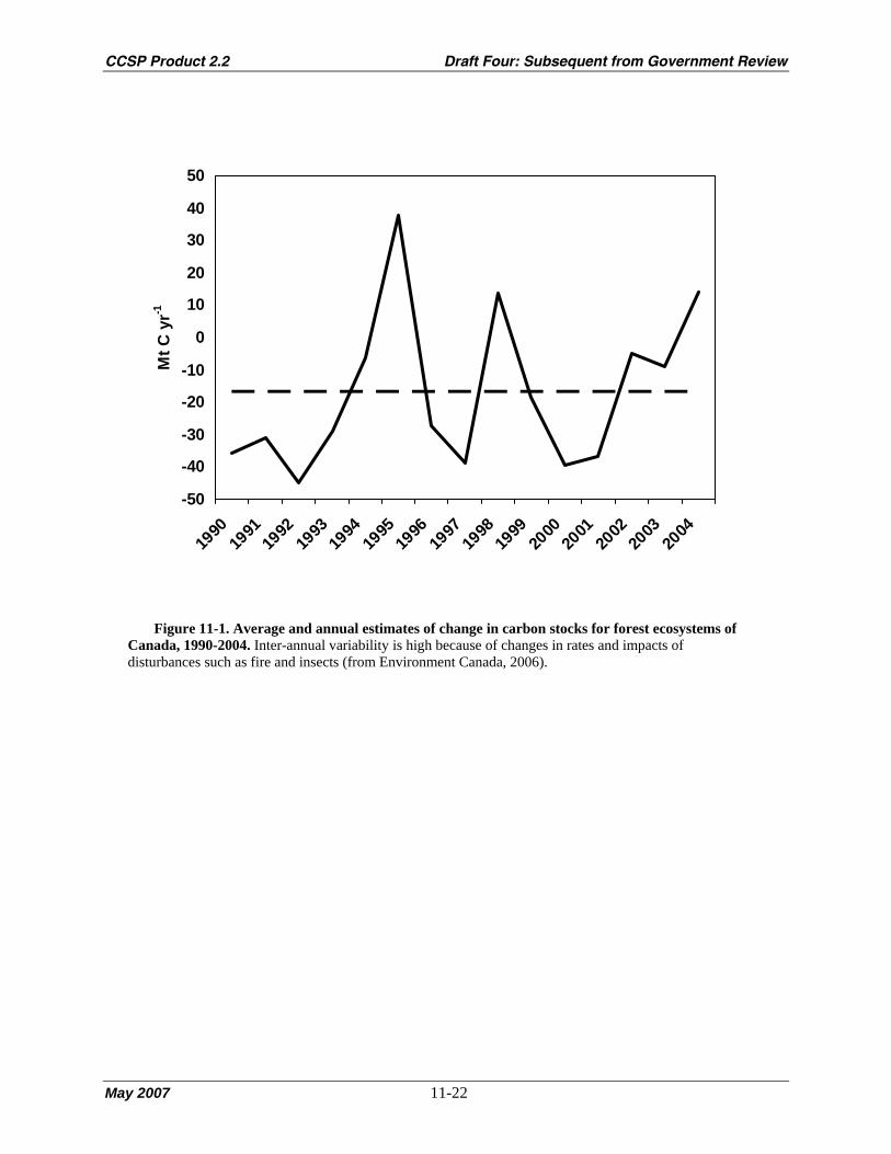
CCSP Product 2.2 Draft Four: Subsequent from Government Review
May 2007 11-22
Figure 11-1. Average and annual estimates of change in carbon stocks for forest ecosystems of Canada, 1990-2004. Inter-annual variability is high because of changes in rates and impacts of disturbances such as fire and insects (from Environment Canada, 2006).
-50
-40
-30
-20
-10
0
10
20
30
40
50
1990
1991
1992
1993
1994
1995
1996
1997
1998
1999
2000
2001
2002
2003
2004
Mt C
yr-1
CCSP Product 2.2 Draft Four: Subsequent from Government Review
May 2007 12-1
Chapter 12. Carbon Cycles in the Permafrost Region
of North America
Lead Author: Charles Tarnocai1
Contributing Authors: Chien-Lu Ping,2 and John Kimble3
1Agriculture and Agri-Food Canada, 2University of Alaska, Fairbanks,
3USDA Natural Resources Conservation Service (retired)
KEY FINDINGS
• Much of northern North America (more than 6 million square kilometers) is characterized by the
presence of permafrost, (soils or rocks that remain frozen for at least two consecutive years). This
permafrost region contains approximately 25% of the world’s total soil organic carbon, a massive pool
of carbon that is vulnerable to release to the atmosphere as carbon dioxide in response to an already
detectable polar warming.
• The soils of the permafrost region of North America contain 213 billion tons of organic carbon,
approximately 61% of the carbon in all soils of North America.
• The soils of the permafrost region of North America are currently a net sink of approximately 11
million tons of carbon per year.
• The soils of the permafrost region of North America have been slowly accumulating carbon for the
last 5000–8000 years. More recently, increased human activity in the region has resulted in
permafrost degradation and at least localized loss of soil carbon.
• Patterns of climate, especially the region’s cool and cold temperatures and their interaction with soil
hydrology to produce wet and frozen soils, are primarily responsible for the historical accumulation of
carbon in the region. Non-climatic drivers of carbon change include human activities, including
flooding associated with hydroelectric development, that degrade permafrost and lead to carbon loss.
Fires, increasingly common in the region, also lead to carbon loss.
• Projections of future warming of the polar regions of North America lead to projections of carbon loss
from the soils of the permafrost region, with upwards of 78% (34 billion tons) and 41% (40 billion tons)
of carbon stored in soils of the Subarctic and northern-most coniferous (boreal) regions, respectively,
being severely or extremely severely affected by future climate change.
• Options for management of carbon in the permafrost region of North America, including construction
methods that cause as little disturbance of the permafrost and surface as possible, are primarily those
which avoid permafrost degradation and subsequent carbon losses.
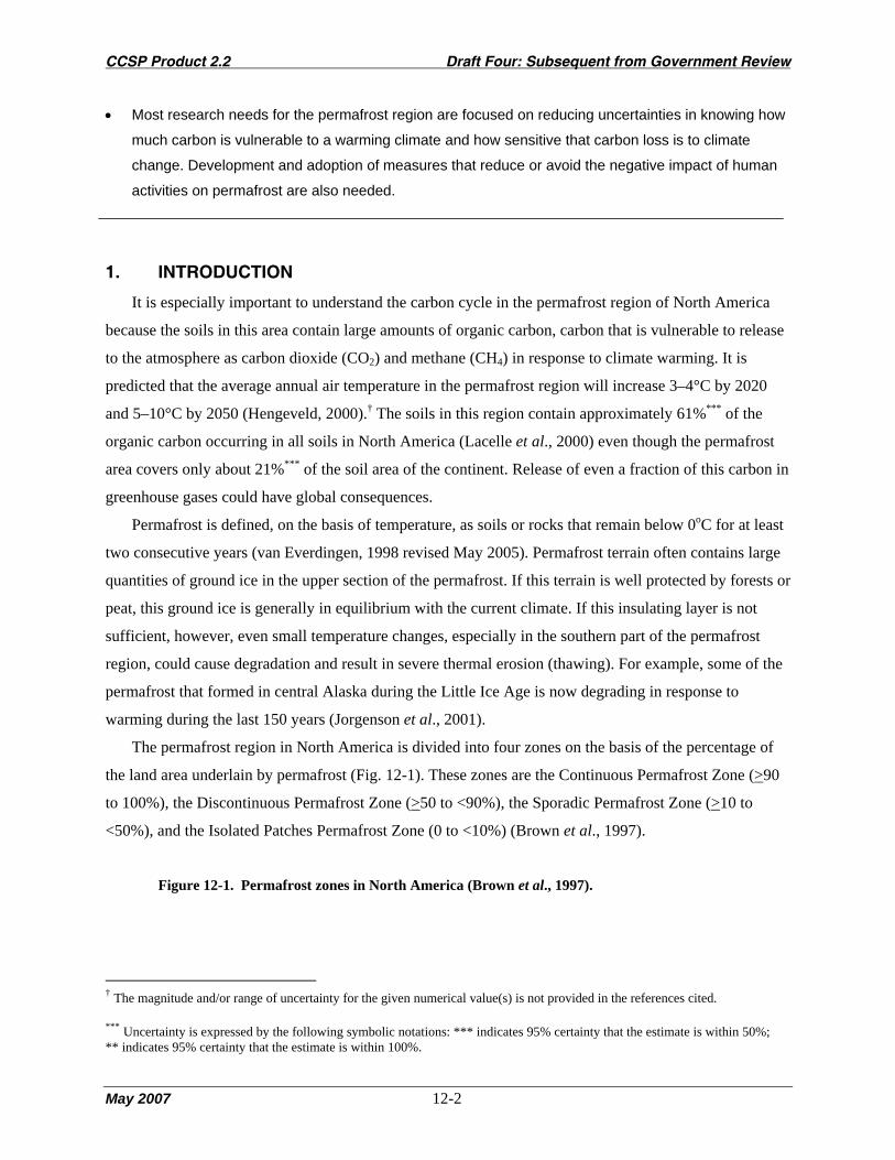
CCSP Product 2.2 Draft Four: Subsequent from Government Review
May 2007 12-2
• Most research needs for the permafrost region are focused on reducing uncertainties in knowing how
much carbon is vulnerable to a warming climate and how sensitive that carbon loss is to climate
change. Development and adoption of measures that reduce or avoid the negative impact of human
activities on permafrost are also needed.
1. INTRODUCTION
It is especially important to understand the carbon cycle in the permafrost region of North America
because the soils in this area contain large amounts of organic carbon, carbon that is vulnerable to release
to the atmosphere as carbon dioxide (CO2) and methane (CH4) in response to climate warming. It is
predicted that the average annual air temperature in the permafrost region will increase 3–4°C by 2020
and 5–10°C by 2050 (Hengeveld, 2000).† The soils in this region contain approximately 61%*** of the
organic carbon occurring in all soils in North America (Lacelle et al., 2000) even though the permafrost
area covers only about 21%*** of the soil area of the continent. Release of even a fraction of this carbon in
greenhouse gases could have global consequences.
Permafrost is defined, on the basis of temperature, as soils or rocks that remain below 0oC for at least
two consecutive years (van Everdingen, 1998 revised May 2005). Permafrost terrain often contains large
quantities of ground ice in the upper section of the permafrost. If this terrain is well protected by forests or
peat, this ground ice is generally in equilibrium with the current climate. If this insulating layer is not
sufficient, however, even small temperature changes, especially in the southern part of the permafrost
region, could cause degradation and result in severe thermal erosion (thawing). For example, some of the
permafrost that formed in central Alaska during the Little Ice Age is now degrading in response to
warming during the last 150 years (Jorgenson et al., 2001).
The permafrost region in North America is divided into four zones on the basis of the percentage of
the land area underlain by permafrost (Fig. 12-1). These zones are the Continuous Permafrost Zone (>90
to 100%), the Discontinuous Permafrost Zone (>50 to <90%), the Sporadic Permafrost Zone (>10 to
<50%), and the Isolated Patches Permafrost Zone (0 to <10%) (Brown et al., 1997).
Figure 12-1. Permafrost zones in North America (Brown et al., 1997).
† The magnitude and/or range of uncertainty for the given numerical value(s) is not provided in the references cited. *** Uncertainty is expressed by the following symbolic notations: *** indicates 95% certainty that the estimate is within 50%; ** indicates 95% certainty that the estimate is within 100%.
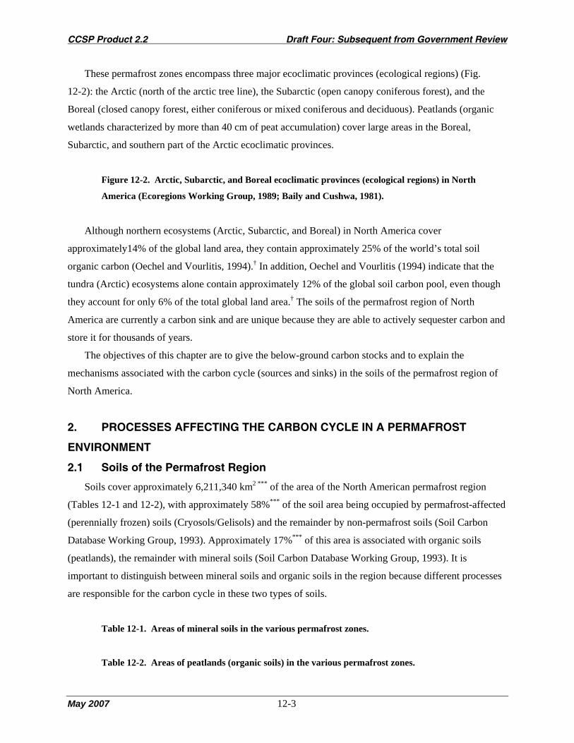
CCSP Product 2.2 Draft Four: Subsequent from Government Review
May 2007 12-3
These permafrost zones encompass three major ecoclimatic provinces (ecological regions) (Fig.
12-2): the Arctic (north of the arctic tree line), the Subarctic (open canopy coniferous forest), and the
Boreal (closed canopy forest, either coniferous or mixed coniferous and deciduous). Peatlands (organic
wetlands characterized by more than 40 cm of peat accumulation) cover large areas in the Boreal,
Subarctic, and southern part of the Arctic ecoclimatic provinces.
Figure 12-2. Arctic, Subarctic, and Boreal ecoclimatic provinces (ecological regions) in North
America (Ecoregions Working Group, 1989; Baily and Cushwa, 1981).
Although northern ecosystems (Arctic, Subarctic, and Boreal) in North America cover
approximately14% of the global land area, they contain approximately 25% of the world’s total soil
organic carbon (Oechel and Vourlitis, 1994).† In addition, Oechel and Vourlitis (1994) indicate that the
tundra (Arctic) ecosystems alone contain approximately 12% of the global soil carbon pool, even though
they account for only 6% of the total global land area.† The soils of the permafrost region of North
America are currently a carbon sink and are unique because they are able to actively sequester carbon and
store it for thousands of years.
The objectives of this chapter are to give the below-ground carbon stocks and to explain the
mechanisms associated with the carbon cycle (sources and sinks) in the soils of the permafrost region of
North America.
2. PROCESSES AFFECTING THE CARBON CYCLE IN A PERMAFROST
ENVIRONMENT
2.1 Soils of the Permafrost Region
Soils cover approximately 6,211,340 km2 *** of the area of the North American permafrost region
(Tables 12-1 and 12-2), with approximately 58%*** of the soil area being occupied by permafrost-affected
(perennially frozen) soils (Cryosols/Gelisols) and the remainder by non-permafrost soils (Soil Carbon
Database Working Group, 1993). Approximately 17%*** of this area is associated with organic soils
(peatlands), the remainder with mineral soils (Soil Carbon Database Working Group, 1993). It is
important to distinguish between mineral soils and organic soils in the region because different processes
are responsible for the carbon cycle in these two types of soils.
Table 12-1. Areas of mineral soils in the various permafrost zones.
Table 12-2. Areas of peatlands (organic soils) in the various permafrost zones.

CCSP Product 2.2 Draft Four: Subsequent from Government Review
May 2007 12-4
2.2 Mineral Soils
The schematic diagram in Fig. 12-3 provides general information about the carbon sinks and sources
in mineral soils. Most of the permafrost-affected mineral soils are carbon sinks because of the process of
cryoturbation, which moves organic matter into the deeper soil layers. Other processes, such as
decomposition, wildfires, and thermal degradation, release carbon into the atmosphere and, thus, act as
carbon sources.
Figure 12-3. Carbon cycle in permafrost-affected upland (mineral) soils, showing below-ground
organic carbon sinks and sources.
For unfrozen soils and noncryoturbated frozen soils in the permafrost region, the carbon cycle is
similar to that in soils occurring in temperate regions. In these soils, organic matter is deposited on the
soil surface. Some soluble organic matter may move downward, but because these soils are not affected
by cryoturbation, they have no mechanism for moving organic matter from the surface into the deeper soil
layers and preserving it from decomposition and wildfires. Most of their below-ground carbon originates
from roots and its residence time is relatively short.
The role of cryoturbation: Although permafrost-affected ecosystems produce much less biomass than
do temperate ecosystems, permafrost-affected soils that are subject to cryoturbation (frost-churning), a
cryogenic process, have a unique ability to sequester a portion of this organic matter and store it for
thousands of years. A number of models have been developed to explain the mechanisms involved in
cryoturbation (Mackay, 1980; Van Vliet-Lanoë, 1991; Vandenberghe, 1992). The most recent model
involves the process of differential frost heave (heave-subsidence), which produces downward and lateral
movement of materials (Walker et al., 2002; Peterson and Krantz, 2003).
Part of the organic matter produced annually by the vegetation is deposited as litter on the soil
surface, with some decomposing as a result of biological activity. A large portion of this litter, however,
builds up on the soil surface, forming an organic soil horizon. Cryoturbation causes some of this organic
material to move down into the deeper soil layers (Bockheim and Tarnocai, 1998). Soluble organic
materials move downward because of the effect of gravity and the movement of water along the thermal
gradient toward the freezing front (Kokelj and Burn, 2005). Once the organic material has moved down to
the cold, deeper soil layers where very little or no biological decomposition takes place, it may be
preserved for many thousands of years. Radiocarbon dates from cryoturbated soil materials ranged
between 490 and 11,200 yr BP (Zoltai et al., 1978). These dates were randomly distributed within the soil

CCSP Product 2.2 Draft Four: Subsequent from Government Review
May 2007 12-5
and did not appear in chronological sequence by depth (the deepest material was not necessarily the
oldest), indicating that cryoturbation is an ongoing process.
The permafrost table (top of the permafrost) is very dynamic and is subject to deepening due to
factors such as removal of vegetation and/or the insulating surface organic layer, wildfires, global climate
change, and other natural or human activities. When this occurs, the seasonally thawed layer (active layer)
becomes deeper and the organic material is able to move even deeper into the soil (translocation).
However, if such factors cause thawing of the soil and melting of the ground ice, some or all of the
organic materials locked in the system could be exposed to the atmosphere. This change in soil
environment gives rise to both aerobic and anaerobic decomposition, releasing carbon into the atmosphere
as carbon dioxide and methane, respectively (Fig. 12-3). At this stage, the soil can become a major carbon
source.
If, however, the permafrost table rises (and the active layer becomes shallower) because of
reestablishment of the vegetation or buildup of the surface organic layer, this deep organic material
becomes part of the permafrost and is, thus, more securely preserved. This is the main reason that
permafrost-affected soils contain high amounts of organic carbon not only in the upper (0–100 cm) layer,
but also in the deeper layers. These cryoturbated, permafrost-affected soils are effective carbon sinks.
2.3 Peatlands (Organic Soils)
The schematic diagram in Fig. 12-4 provides general information about the processes driving the
carbon sinks and sources in peatland soils. The water-saturated conditions, low soil temperatures, and
acidic conditions of northern peatlands provide an environment in which very little decomposition occurs;
hence, the litter is converted to peat and preserved. This gradual buildup process has been ongoing in
peatlands during the last 5000–8000 years, resulting in peat deposits that are an average of 2–3 m thick
and, in some cases, up to 10 m thick. At this stage, peatlands can act as very effective carbon sinks for
many thousands of years (Fig. 12-4).
Figure 12-4. Carbon cycle in permafrost peatlands, showing below-ground organic carbon sinks and
sources.
Carbon dynamics: Data for carbon accumulation in various peatland types in the permafrost regions
are given in Table 12-3. Although some values for the rate of peat accumulation are higher (associated
with unfrozen peatlands), the value for frozen peatlands, which are more widespread, is 13.31 ± 2.20 g C
m-2 yr-1 (Robinson and Moore, 1999). Peat accumulations in the various ecological regions were
calculated on the basis of the thickness of the deposit and the date of the basal peat. The rate of peat

CCSP Product 2.2 Draft Four: Subsequent from Government Review
May 2007 12-6
accumulation is generally highest in the Boreal region and decreases northward (Table 12-3). Note,
however, that if the surface of the peat deposit has eroded, the calculated rate of accumulation (based on
the age of the basal peat and a decreased deposit thickness) will appear to be higher than it should be.
This is probably the reason for some of the high rates of peat accumulation found for the Arctic region,
which likely experienced a rapid rate of accumulation during the Hypsithermal Maximum with
subsequent erosion of the surface of some of the deposits reducing their thicknesses. Wildfires,
decomposition, and leaching of soluble organic compounds release approximately one-third of the carbon
input, causing most of the carbon loss in these peatlands.
Table 12-3. Organic carbon accumulation and loss in various Canadian peatlands. Positive values
indicate net flux into the atmosphere (source); negative values indicate carbon sequestration (land sinks).
3. BELOW-GROUND CARBON STOCKS
The carbon content of mineral soils to a 1-m depth is 49-61 kg m-2 for permafrost-affected soils and
12-17 kg m-2 for unfrozen soils (Tables 12-4 and 12-5). The carbon content of organic soils (peatlands)
for the total depth of the deposit is 81-129 kg m-2 for permafrost-affected soils and 43-144 kg m-2 for
unfrozen soils (Tables 12-4 and 12-5) (Tarnocai, 1998 and 2000).
Table 12-4. Soil carbon pools and fluxes for the permafrost areas of Canada. Positive flux numbers
indicate net flux into the atmosphere (source); negative values indicate carbon sequestration (land sinks).
Table 12-5. Average organic carbon content for soils in the various ecological regions (Tarnocai 1998
and 2000).
Soils in the permafrost region of North America contain 213 Gt of organic carbon (Tables 12-6 and
12-7), which is approximately 61% of the organic carbon in all soils on this continent (Lacelle et al.,
2000). Mineral soils contain approximately 99 Gt of organic carbon in the 0- to 100-cm depth
(Table 12-6). Although peatlands (organic soils) cover a smaller area than mineral soils (17% vs 83%),
they contain approximately 114 Gt of organic carbon in the total depth of the deposit, or more than half
(54%) of the soil organic carbon of the region (Table 12-7).
Table 12-6. Organic carbon mass in mineral soils in the various permafrost zones.
Table 12-7. Organic carbon mass in peatlands (organic soils) in the various permafrost zones.

CCSP Product 2.2 Draft Four: Subsequent from Government Review
May 2007 12-7
4. CARBON FLUXES
4.1 Mineral Soils
Very little information is available about carbon fluxes in both unfrozen and perennially frozen
mineral soils in the permafrost regions. For unfrozen upland mineral soils, Trumbore and Harden (1997)
report a carbon accumulation of 60-100 g C m-2 yr-1 (Table 12-4). They further indicate that the slow
decomposition results in rapid organic matter accumulation, but the turnover time due to wildfires (every
500–1000 years) eliminates the accumulated carbon except for the deep carbon derived from roots in the
subsoil. The turnover time for this deep carbon is 100-1600 years. Therefore, the carbon stocks in these
unfrozen soils are low, and the turnover time of this carbon is 100 to 1000 years.
As with unfrozen mineral soils, very little information has been published on the carbon cycle in
perennially frozen mineral soils. The carbon cycle in these soils differs from that in unfrozen soils in that,
because of cryogenic activities, these soils are able to move the organic matter deposited on the soil
surface into the deeper soil layers. Assuming that cryoturbation was active in these soils during the last
six thousand years (Zoltai et al., 1978), an average of 9 Mt C** have been added annually to these soils.
Most of this carbon has been cryoturbated into the deeper soil layers, but some of the carbon in the
surface organic layer is released by decomposition and, periodically, by wildfires. The schematic diagram
in Fig. 12-5 shows the carbon cycle in these soils.
Figure 12-5. Carbon cycle in perennially frozen mineral soils in the permafrost region.
4.2 Peatlands (Organic Soils)
Peatland vegetation deposits various amounts of organic material (litter) annually on the peatland
surface. Reader and Stewart (1972) found that the amount of litter (dry biomass) deposited annually on
the bog surface in Boreal peatlands in Manitoba, Canada was 489-1750 g m-2. Approximately 25% of the
original litter fall was found to have decomposed during the following year. In the course of the study,
they found that the average annual accumulation rate was 10% of the annual net primary production.
Robinson and Moore (1999) and Robinson et al. (2003) found that, in the Sporadic Permafrost Zone,
mean carbon accumulation rates over the past 100 years for unfrozen bogs and frost mounds were 88.6 ±
4.4 and 78.5 ± 8.8 g m-2 yr-1, respectively. They also found that, in the Discontinuous Permafrost Zone,
the mean carbon accumulation rate during the past 1200 years in frozen peat plateaus was 13.31 ± 2.20 g
m-2 yr-1, while in unfrozen fens and bogs the comparable rates were 20.34 ± 2.86 and 21.81 ± 3.25 g m-2
yr-1, respectively.
Because peatlands cover large areas in the permafrost region of North America, their contribution to
the carbon stocks is significant (Table 12-5). Zoltai et al. (1988) estimated that the annual carbon

CCSP Product 2.2 Draft Four: Subsequent from Government Review
May 2007 12-8
accumulation capacity of Boreal peatlands is approximately 9.8 Mt.† Gorham (1988), in contrast,
estimated that Canadian peatlands accumulate approximately 30 Mt C† annually.
Currently, wildfires are probably the greatest natural force in converting peatlands to a carbon source.
Ritchie (1987) found that the western Canadian Boreal forests have a fire return interval of 50-100 years,
while Kuhry (1994) indicated that, for wetter Sphagnum bogs, the interval is 400-1700 years. For peat
plateau bogs, each fire resulted in an average decrease in carbon mass of 1.46 kg m-2 and an average
decrease in height of 2.74 cm, which represents about 150 years of peat accumulation (Robinson and
Moore, 2000). In recent years, the number of these wildfires has increased, as has the area burned,
releasing increasing amounts of carbon into the atmosphere.
The schematic diagram presented in Fig. 12-6 summarizes the carbon cycle in peatlands in the
permafrost region. Based on average values for the rate of peat accumulation, approximately 17 g C m-2
yr-1, or 18 Mt C, is added annually to peatlands in this region of North America. Approximately 1.46 kg C
m-2 is released to the atmosphere every 600 years by wildfires in the northern boreal peatlands. In
addition, decomposition of unfrozen peatlands releases approximately 2.0 g C m-2 yr-1, and a further 2.0 g
C m-2 yr-1 is released by leaching of dissolved organic carbon (DOC), leading to a carbon decrease of
approximately 4 Mt** annually, not including that released by wildfires (Fig. 12-6). Note that these values
are based on current measurements. However, rates of peat accumulation have varied during the past
6000–8000 years, with periods during which the rate of peat accumulation was much higher than at
present.
Figure 12-6. Carbon cycle in peatlands in the permafrost region.
4.3 Total Flux
Based on the limited data available for this vast, and largely inaccessible, area of the continent,
approximately 27 Mt C per year** is deposited on the surface of mineral soils and peatlands (organic soils)
in the permafrost region of North America. Approximately 8 Mt per year** of surface carbon (excluding
vegetation) is released by decomposition and wildfires, and by leaching into the water systems. Thus, the
soils in the permafrost region of North America currently act as a sink for approximately 19 Mt C per
year** and as a source for approximately 8 Mt C per year** and are, therefore, a net carbon sink
(Figs. 12-5 and 12-6).
5. POSSIBLE EFFECTS OF GLOBAL CLIMATE CHANGE
The permafrost region is unique because the soils in this vast area contain large amounts of organic
materials and much of the carbon has been actively sequestered by peat accumulation (organic soils) and

CCSP Product 2.2 Draft Four: Subsequent from Government Review
May 2007 12-9
cryoturbation (mineral soils) and stored in the permafrost for many thousands of years. Historical patterns
of climate are responsible for the large amount of carbon found in the soils of the region today, but
cryoturbation is a consequence of the region’s current cool to cold climate and the effects of that climate
on soil hydrology. As a result, patterns of climate and climate change are dominant drivers of carbon
cycling in the region. Future climate change will determine the fate of that carbon and whether the region
will remain a slow but significant carbon sink, or whether it will reverse and become a source, rapidly
releasing large amounts of carbon dioxide (CO2) and methane (CH4) to the atmosphere.
5.1 Peatlands
A model for estimating the sensitivity of peatlands to global climate change was developed using
current climate (1x CO2), vegetation, and permafrost data together with the changes in these variables
expected in a 2x CO2 environment (Kettles and Tarnocai, 1999). The data generated by this model were
used to produce a peatland sensitivity map. Using GIS techniques, this map was overlaid on the peatland
map of Canada to determine both the sensitivity ratings of the various peatland areas and the associated
organic carbon masses. The sensitivity ratings, or classes, used are no change, very slight, slight,
moderate, severe, and extremely severe. Because global climate change is expected to have the greatest
impact on the ecological processes and permafrost distribution in peatlands in the severe and extremely
severe categories (Kettles and Tarnocai, 1999), the areas and carbon masses of peatlands in these two
sensitivity classes are considered to be most vulnerable to climate change. The sensitivity ratings are
determined by the degree of change in the ecological zonation combined with the degree of change in the
permafrost zonation, with the greater the change, the more severe the sensitivity rating. For example, if a
portion of the Subarctic becomes Boreal in ecology and the associated sporadic permafrost disappears (no
permafrost remains in the region), the sensitivity of this region is rated as extremely severe. If however, a
portion of the Boreal remains Boreal in ecology, but the discontinuous permafrost disappears (no
permafrost remains in the region), the sensitivity of this region is rated as severe.
The peatland sensitivity model (Tarnocai, 2006) indicates that the greatest effect of global climate
change will occur in the Subarctic region, where about 85% (314,270 km2) of the peatland area and 78%
(33.96 Gt) of the organic carbon mass will be severely or extremely severely affected by climate change,
with 66% of the area and 57% of the organic carbon mass being extremely severely affected (Fig. 12-7).†
The second largest effect will occur in the Boreal region, where about 49% (353,100 km2) of the peatland
area and 41% (40.20 Gt) of the organic carbon mass will be severely or extremely severely affected, with
10% of both the area and organic carbon mass being extremely severely affected. These two regions
contain almost all (99%) of the Canadian peatland area and organic carbon mass that is predicted to be
severely or extremely severely affected (Fig. 12-7) (Tarnocai, 2006).
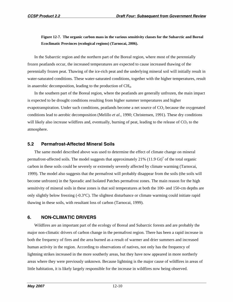
CCSP Product 2.2 Draft Four: Subsequent from Government Review
May 2007 12-10
Figure 12-7. The organic carbon mass in the various sensitivity classes for the Subarctic and Boreal
Ecoclimatic Provinces (ecological regions) (Tarnocai, 2006).
In the Subarctic region and the northern part of the Boreal region, where most of the perennially
frozen peatlands occur, the increased temperatures are expected to cause increased thawing of the
perennially frozen peat. Thawing of the ice-rich peat and the underlying mineral soil will initially result in
water-saturated conditions. These water-saturated conditions, together with the higher temperatures, result
in anaerobic decomposition, leading to the production of CH4.
In the southern part of the Boreal region, where the peatlands are generally unfrozen, the main impact
is expected to be drought conditions resulting from higher summer temperatures and higher
evapotranspiration. Under such conditions, peatlands become a net source of CO2 because the oxygenated
conditions lead to aerobic decomposition (Melillo et al., 1990; Christensen, 1991). These dry conditions
will likely also increase wildfires and, eventually, burning of peat, leading to the release of CO2 to the
atmosphere.
5.2 Permafrost-Affected Mineral Soils
The same model described above was used to determine the effect of climate change on mineral
permafrost-affected soils. The model suggests that approximately 21% (11.9 Gt)† of the total organic
carbon in these soils could be severely or extremely severely affected by climate warming (Tarnocai,
1999). The model also suggests that the permafrost will probably disappear from the soils (the soils will
become unfrozen) in the Sporadic and Isolated Patches permafrost zones. The main reason for the high
sensitivity of mineral soils in these zones is that soil temperatures at both the 100- and 150-cm depths are
only slightly below freezing (-0.3°C). The slightest disturbance or climate warming could initiate rapid
thawing in these soils, with resultant loss of carbon (Tarnocai, 1999).
6. NON-CLIMATIC DRIVERS
Wildfires are an important part of the ecology of Boreal and Subarctic forests and are probably the
major non-climatic drivers of carbon change in the permafrost region. There has been a rapid increase in
both the frequency of fires and the area burned as a result of warmer and drier summers and increased
human activity in the region. According to observations of natives, not only has the frequency of
lightning strikes increased in the more southerly areas, but they have now appeared in more northerly
areas where they were previously unknown. Because lightning is the major cause of wildfires in areas of
little habitation, it is likely largely responsible for the increase in wildfires now being observed.

CCSP Product 2.2 Draft Four: Subsequent from Government Review
May 2007 12-11
Increased human activity as a result of the construction of pipelines, roads, airstrips, and mines,
expansion of agriculture, and development and expansion of town sites has disturbed the natural soil
cover and exposed the organic-rich soil layers, leading to increased soil temperatures and, hence,
decomposition of the exposed organic materials. Burgess and Tarnocai (1997), studying the Norman
Wells Pipeline, provide some examples of the effect of pipeline construction on frozen peatlands and
permafrost in Canada.
Shoreline erosion along rivers, lakes, and oceans and thermal erosion (thermokarst) are also common
processes in the permafrost region, exposing the carbon-rich frozen soil layers to the atmosphere and
making the organic materials available for decomposition. As a result, carbon is released into the
atmosphere as either CO2 or methane, or it enters the water system as dissolved organic carbon.
Large hydroelectric projects in northern areas, such as Southern Indian Lake in Manitoba and the
James Bay region of Quebec, have flooded vast areas of peatlands and initiated permafrost degradation
and decomposition of organic carbon, some of which is released into the atmosphere as methane. Of
greater immediate concern, however, is the carbon that has entered the water system as dissolved organic
carbon. These compounds include contaminants such as persistent organic pollutants [e.g., PCBs, DDT,
HCH, and chlorobenzene (AMAP, 2004)] that have been widely distributed in northern ecosystems over
many years, much of it deposited by snowfalls, concentrated by cryoturbation, and stored in the organic
soils. Of particular concern is the release of methylmercury because peatlands are net producers of this
compound (Driscoll et al., 1998; Suchanek et al., 2000), which is a much greater health hazard than
inorganic or elemental mercury. Natives in the regions where these hydroelectric developments have
taken place have developed mercury poisoning after ingesting fish contaminated by this mercury, leading
to serious health problems for many of the people. This is an example of what can happen when
permafrost degrades as a result of human activities. When climate warming occurs, the widespread
degradation of permafrost, with the resulting release of such dangerous pollutants into the water systems,
could cause serious health problems for fish, animals, and humans that rely on such waters.
7. OPTIONS FOR MANAGEMENT OF CARBON IN THE PERMAFROST REGION
Although wildfires are the most effective mechanism for releasing carbon into the atmosphere, they
are also an important factor in maintaining the integrity of northern ecosystems. Therefore, such fires are
allowed to burn naturally and are controlled only if they are close to settlements or other manmade
structures.
The construction methods currently used in permafrost terrain are designed to cause as little surface
disturbance as possible and to preserve the permafrost. Thus, the construction of pipelines, airstrips, and

CCSP Product 2.2 Draft Four: Subsequent from Government Review
May 2007 12-12
highways is commonly carried out in the winter so that the heavy equipment used will cause minimal
surface disturbance.
The greatest threat to the region is a warmer (and possibly drier) climate, which would drastically
affect not only the carbon cycle, but also the biological systems, including human life. Unfortunately, we
know very little about how to manage the natural systems in this new environment.
8. DATA GAPS AND UNCERTAINTIES
The permafrost environment is a very complex system, and the data available for it are very limited
with numerous gaps and uncertainties. Information on the distribution of soils in the permafrost region is
based on small-scale maps, and the carbon stocks calculated for these soils are derived from a relatively
small number of datasets. Although there is some understanding of the carbon sinks and sources in these
soils, the limited amount of data available make it very difficult, or impossible, to assign reliable values.
Only limited amounts of flux data have been collected for the permafrost-affected soils and, in some
cases, it has been collected on sites that are not representative of the overall landscape. This makes it very
difficult to scale this information up for a larger area. As Davidson and Janssens (2006) state:
“…the unresolved question regarding peatlands and permafrost is not the degree to which the
currently constrained decomposition rates are temperature sensitive, but rather how much
permafrost is likely to melt and how much of the peatland area is likely to dry significantly. Such
regional changes in temperature, precipitation, and drainage are still difficult to predict in global
circulation models. Hence, the climate change predictions, as much as our understanding of carbon
dynamics, limit our ability to predict the magnitude of likely vulnerability of peat and permafrost
carbon to climate change.”
To obtain more reliable estimates of the carbon sinks and sources in permafrost-affected soils, we
need much more detailed data on the distribution and characteristics of these soils. Carbon stock estimates
currently exist only for the upper 1 m of the soil. Limited data from the Mackenzie River Valley in
Canada indicate that a considerable amount of soil organic carbon occurs below the 1-m depth, even at
the 3-m depth. Future estimates of carbon stocks should be extended to cover a depth of 0-2 m or, in some
cases, even greater depths. More measurements of carbon fluxes and inputs are also needed if we are to
understand the carbon sequestration process in these soils in the various permafrost zones. Our
understanding of the effect that rapid climate warming will have on the carbon sinks and sources in these
soils is also very limited. Future research should focus in greater detail on how the interactions of climate
with the biological and physical environments will affect the carbon balance in permafrost-affected soils.

CCSP Product 2.2 Draft Four: Subsequent from Government Review
May 2007 12-13
The changes that are occurring, and will occur, in the permafrost region are almost totally driven by
natural forces and so are almost impossible for humans to manage on a large scale. Human activities, such
as they are, are aimed at protecting the permafrost and, thus, preserving the carbon. Perhaps we humans
should realize that there are systems (e.g., glaciers, ocean currents, droughts, and rainfall) that will be
impossible for us to manage. We simply must learn to accept them, and if possible, adapt.
CHAPTER 12 REFERENCES
AMAP, 2004: AMAP Assessment 2002: Persistent Organic Pollutants in the Arctic. Oslo, Arctic Monitoring and
Assessment Programme, xvi+310 pp.
Bailey, R. and C.T. Cushwa, 1981: Ecoregions of North America. 1:12 million scale map, U.S. Forest Service and
U.S. Fish and Wildlife Service.
Bockheim, J.G. and C. Tarnocai, 1998: Recognition of cryoturbation for classifying permafrost-affected soils.
Geoderma, 81, 281-293.
Brown, J., O.J. Ferrians, Jr., J.A. Heginbottom, and E.S. Melnikov, 1997: Circum-Arctic Map of Permafrost and
Ground Ice Conditions. 1:10 million scale map, International Permafrost Association.
Burgess, M.M. and C. Tarnocai, 1997: Peatlands in the discontinuous permafrost zone along the Norman Wells
pipeline, Canada. In: Proceedings of the International Symposium on Physics, Chemistry, and Ecology of
Seasonally Frozen Soils Fairbanks, Alaska, June 10-12, 1997 [Iskandr, I.K., E.A. Wright, J.K. Radke, B.S.
Sharratt, P.H. Groenevelt, and L.D. Hinzman (eds.)]. Special Report 97-10, U.S. Army Cold Regions Research
and Engineering Laboratory, Hanover, USA, pp. 417-424.
Christensen, T., 1991: Arctic and sub-Arctic soil emissions: possible implications for global climate change. Polar
Record, 27, 205-210.
Cryosol Working Group, 2001: Northern and Mid Latitudes Soil Database, Version 1. National Soil Database,
Research Branch, Agriculture and Agri-Food Canada, Ottawa, Ontario, Canada.
Davidson, E.A. and I.A. Janssens, 2006: Temperature sensitivity of soil carbon decomposition and feedbacks to
climate change. Nature, 440, 165-173.
Driscoll, C.T., J. Holsapple, C.L. Schofield, and R. Munson, 1998: The chemistry and transport of mercury in a
small wetland in the Adirondack region of New York, USA. Biogeochemistry, 40, 137-146.
Ecoregions Working Group, 1989: Ecoclimatic Regions of Canada, First Approximation. Ecoregions Working
Group of the Canada Committee on Ecological Land Classification, Ecological Land Classification Series, No.
23, 119 pp. and map, Sustainable Development Branch, Canadian Wildlife Service, Conservation and
Protection, Environment Canada, Ottawa, Ontario, Canada.
Gorham, E., 1988: Canada’s peatlands: their importance for the global carbon cycle and possible effect of
“greenhouse” climate warming. Transactions of the Royal Society of Canada, Series V, 3, 21-23.

CCSP Product 2.2 Draft Four: Subsequent from Government Review
May 2007 12-14
Hengeveld, H.G., 2000: Projections for Canada’s climate future: a discussion of recent simulations with the
Canadian Global Climate Model. In: Climate Change Digest. CCD 00-01, Special Edition, 27 pp. Last accessed
April 6, 2005, Meteorological Service of Canada, Environment Canada, Downsview, Ontario, Canada.
Available at http://www.msc.ec.gc.ca/saib/climate/docs/ccd_00-01.pdf
Jorgenson, M.T., C.H. Racine, J.C. Walters, and T.E. Osterkamp, 2001: Permafrost degradation and ecological
changes associated with a warming climate in central Alaska. Climate Change, 48, 551-579.
Kettles, I.M. and C. Tarnocai, 1999: Development of a model for estimating the sensitivity of Canadian peatlands to
climate warming. Geographie physique et Quaternaire, 53, 323-338.
Kokelj, S.V. and C.R. Burn, 2005: Geochemistry of the active layer and near-surface permafrost, Mackenzie delta
region, Northwest Territories, Canada. Canadian Journal of Earth Sciences, 42, 37-48.
Kuhry, G.P., 1994: The role of fire in the development of Sphagnum-dominated peatlands in the western boreal
Canada. Journal of Ecology, 82, 899-910.
Lacelle, B., C. Tarnocai, S. Waltman, J. Kimble, N. Bliss, B. Worstell, F. Orozco-Chavez, and B. Jakobsen, 2000:
North American Soil Organic Carbon Map. 1:10 million scale map, Agriculture and Agri-Food Canada, USDA,
USGS, INEGI and Institute of Geography, University of Copenhagen.
Liblik, L.K., T.R. Moore, J.L. Bubier, and S.D. Robinson, 1997: Methane emissions from wetlands in the zone of
discontinuous permafrost: Fort Simpson, Northwest Territories, Canada. Global Biogeochemical Cycles, 11,
485-494.
Mackay, J.R., 1980: The origin of hummocks, western Arctic coast, Canada. Canadian Journal of Earth Sciences,
13, 889-897.
Melillo, J.M., T.V. Callaghan, F.I. Woodward, E. Salati, and S.K. Sinha, 1990: Effects on ecosystems (Chapter 10).
In: Climate Change: The IPCC Scientific Assessment [Houghton, J.T., G.J. Jenkins, and J.J. Ephraums (eds.)].
Cambridge University Press, Cambridge, UK, pp. 283-310.
Moore, T.R., 1997: Dissolved organic carbon: sources, sinks, and fluxes and role in the soil carbon cycle (Chapter
19). In: Soil Processes and the Carbon Cycle [Lal, R., J.M. Kimble, R.F. Follett, and B.A. Stewart (eds.)].
Advances in Soil Science, CRC Press, Boca Raton, FL, pp. 281-292.
Moore, T.R. and N.T. Roulet, 1995: Methane emissions from Canadian peatlands (Chapter 12). In: Soils and Global
Change [Lal, R., J. Kimble, E. Levine, and B.A. Stewart (eds.)]. CRC Lewis Publishers, Boca Raton, FL, pp.
153-164.
National Wetlands Working Group, 1988: Wetlands of Canada. Ecological Land Classification Series No. 24,
Polyscience Publications, Ltd, Sustainable Development Branch, Environment Canada and Montreal, Ottawa,
Canada, 452 pp.
Oechel, W. and G.L. Vourlitis, 1994: The effect of climate change on land-atmosphere feedbacks in arctic tundra
regions. Trends in Ecology and Evolution, 9, 324-329.
Peterson, R.A. and W.B. Krantz, 2003: A mechanism for differential frost heave and its implications for patterned-
ground formation. Journal of Glaciology, 49(164), 69-80.

CCSP Product 2.2 Draft Four: Subsequent from Government Review
May 2007 12-15
Reader, R.J. and J.M. Stewart, 1972: The relationship between net primary production and accumulation for a
peatland in southeastern Manitoba. Ecology, 53, 1024-1037.
Ritchie, J.C., 1987: Postglacial Vegetation of Canada. Cambridge University Press, New York, NY, 178 pp.
Robinson, S.D. and T.R. Moore, 1999: Carbon and peat accumulation over the past 1200 years in a landscape with
discontinuous permafrost, northwestern Canada. Global Biogeochemical Cycles, 13, 591-601.
Robinson, S.D. and T.R. Moore, 2000: The influence of permafrost and fire upon carbon accumulation in High
Boreal peatlands, Northwest Territories, Canada. Arctic, Antarctic, and Alpine Research, 32(2), 155-166.
Robinson, S.D., M.R. Turetsky, I.M. Kettles, and R.K. Wieder, 2003: Permafrost and peatland carbon sink capacity
with increasing latitude. In: Proceedings of the 8th International Conference on Permafrost [Phillips, M., S.M.
Springman, and L.U. Arenson (eds.)]. Zurich, Switzerland, 2, 965-970, Balkema Publishers, Lisse, The
Netherlands.
Soil Carbon Database Working Group, 1993: Soil Carbon for Canadian Soils. Digital database, Centre for Land
and Biological Resources Research, Research Branch, Agriculture and Agri-Food Canada, Ottawa, Ontario,
Canada.
Suchanek, T.H., P.J. Richerson, J.R. Flanders, D.C. Nelson, L.H. Mullen, L.L. Brester, and J.C. Becker, 2000:
Monitoring inter-annual variability reveals sources of mercury contamination in Clear Lake, CA. Environmental
Monitoring and Assessment, 64, 299-310.
Tarnocai, C., 1998: The amount of organic carbon in various soil orders and ecological provinces in Canada. In:
Soil Processes and the Carbon Cycle [Lal, R., J.M. Kimble, R.L.F. Follett, and B.A. Stewart (eds.)]. Advances
in Soil Science, CRC Press, New York, NY, 81-92.
Tarnocai, C., 1999: The effect of climate warming on the carbon balance of Cryosols in Canada. In: Cryosols and
Cryogenic Environments [Tarnocai, C., R. King, and S. Smith (eds.)]. Special issue of Permafrost and
Periglacial Processes, 10(3), 251-263.
Tarnocai, C., 2000: Carbon pools in soils of the Arctic, Subarctic and Boreal regions of Canada. In: Global Climate
Change and Cold Regions Ecosystems [Lal, R., J.M. Kimble, and B.A. Stewart (eds.)]. Advances in Soil
Science, Lewis Publishers, Boca Raton, FL, pp. 91-103.
Tarnocai, C., 2006: The effect of climate change on carbon in Canadian peatlands. Global and Planetary Change,
53, 222-232.
Tarnocai, C., I.M. Kettles, and B. Lacelle, 2005: Peatlands of Canada Database. Digital database, Research
Branch, Agriculture and Agri-Food Canada, Ottawa, Ontario, Canada.
Trumbore, S.E. and J.W. Harden, 1997: Accumulation and turnover of carbon in organic and mineral soils of the
BOREAS northern study area. Journal of Geophysical Research, 102(D24), 28,817-28,830.
Turetsky, M.R., B.D. Amiro, E. Bosch, and J.S. Bhatti, 2004: Historical burn area in western Canadian peatlands
and its relationship to fire weather indices. Global Biogeochemical Cycles, 18, GB4014,
doi:10.1029/2004GB002222.
Vandenberghe, J., 1992: Cryoturbations: a sediment structural analysis. Permafrost and Periglacial Processes, 4,
121-135.

CCSP Product 2.2 Draft Four: Subsequent from Government Review
May 2007 12-16
van Everdingen, R. (ed.), 1998 revised May 2005: Multi-language Glossary of Permafrost and Related Ground-Ice
Terms. National Snow and Ice Data Center/World Data Center for Glaciology, 90 pp., Boulder, CO. Available
at http://nsidc.org/fgdc/glossary
Van Vliet-Lanoë, B., 1991: Differential frost heave, load casting and convection: converging mechanisms; a
discussion of the origin of cryoturbations. Permafrost and Periglacial Processes, 2, 123-139.
Vitt, D.H., L.A. Halsey, I.E. Bauer, and C. Campbell, 2000: Spatial and temporal trends in carbon storage of
peatlands of continental western Canada through the Holocene. Canadian Journal of Earth Sciences, 37, 683-
693.
Walker, D.A., V.E. Romanovsky, W.B. Krantz, C.L. Ping, R.A. Peterson, M.K. Raynolds, H.E. Epstein, J.G. Jia,
and D.C. Wirth, 2002: Biocomplexity of Frost Boil Ecosystem on the Arctic Slope, Alaska. ARCUS 14th Annual
Meeting and Arctic Forum 2002, Arlington, VA, USA. Available at
http://siempre.arcus.org/4DACTION/wi_pos_displayAbstract/5/391
Zoltai, S.C., C. Tarnocai, and W.W. Pettapiece, 1978: Age of cryoturbated organic material in earth hummocks
from the Canadian arctic. Proceedings of the Third International Conference on Permafrost, Edmonton, Alberta,
Canada, pp. 325-331.
Zoltai, S.C., S. Taylor, J.K. Jeglum, G.F. Mills, and J.D. Johnson, 1988: Wetlands of Boreal Canada. In: Wetlands
of Canada. Ecological Land Classification Series, No. 24, National Wetlands Working Group, Sustainable
Development Branch, Environment Canada, Ottawa, Canada, and Polyscience Publications, Montreal, Quebec,
Canada, pp. 97-154.

CCSP Product 2.2 Draft Four: Subsequent from Government Review
May 2007 12-17
Table 12-1. Areas of mineral soils in the various permafrost zones
Area (103 km2) Permafrost zones Canadaa Alaskab Total
Continuous 2001.80 353.46 2355.26 Discontinuous 636.63 479.15 1115.78 Sporadic 717.63 110.98 828.61 Isolated Patches 868.08 0.73 868.81
Total 4224.14 944.32 5168.46 aCalculated using the Soil Carbon of Canada Database (Soil Carbon Database
Working Group, 1993). bCalculated using the Northern and Mid Latitudes Soil Database (Cryosol Working
Group, 2001).
Table 12-2. Areas of peatlands (organic soils) in the various permafrost zones
Area (103 km2) Permafrost zones Canadaa Alaskab Total
Continuous 176.70 51.31 228.01 Discontinuous 243.51 28.74 272.25 Sporadic 307.72 0.62 308.34 Isolated Patches 221.23 13.05 234.28
Total 949.16 93.72 1042.88 aCalculated using the Peatlands of Canada Database (Tarnocai et al., 2005). bCalculated using the Northern and Mid Latitudes Soil Database (Cryosol
Working Group, 2001).

CCSP Product 2.2 Draft Four: Subsequent from Government Review
May 2007 12-18
Table 12-3. Organic carbon accumulation and loss in various Canadian peatlands. Positive values indicate net flux into the atmosphere (source); negative values
indicate carbon sequestration (land sinks)
Peatlands Amount of carbon
Boreal peatlands –9.8 Mt yr–1a
All Canadian peatlands –30 Mt yr–1b
All mineral and organic soils –18 mg m–2 yr–1c
Rich fens –13.58 ± 1.07 g m–2 yr–1d
Poor fens (unfrozen, Discontinuous Permafrost Zone) –20.34 ± 2.86 g m–2 yr–1d
Peat plateaus (frozen, Discontinuous Permafrost Zone) –13.31 ± 2.20 g m–2 yr–1d
Collapse fens –13.54 ± 1.50 g m–2 yr–1d
Bogs (unfrozen, Discontinuous Permafrost Zone) –21.81 ± 3.25 g m–2 yr–1d
Dissolved organic carbon (DOC) +2 g m–2 yr–1e
Arctic peatlands –0 to –16 cm/100 yrf
Subarctic peatlands –2 to –5 cm/100 yrf
Boreal peatlands –2 to –11 cm/100 yrf
Carbon release by each fire in northern boreal peatlands +1.46 kg C m–2g
Carbon release by fires in all terrain +27 Mt yr–1h
Carbon release by fires in Western Canadian peatlands +5.9 Mt yr–1h
aZoltai et al., 1988. bGorham, 1988. cLiblik et al., 1997. dRobinson and Moore, 1999. eMoore, 1997. fCalculated based on the thickness of the deposit and the date of the basal peat (National Wetlands
Working Group, 1988). gRobinson and Moore, 2000. hTuretsky et al., 2004.
Note: Except as explicitly indicated otherwise, no estimates of the confidence, certainty, or uncertainty of the numerical values in this table are available.

CCSP Product 2.2 Draft Four: Subsequent from Government Review
May 2007 12-19
Table 12-4. Soil carbon pools and fluxes for the permafrost areas of Canada. Positive flux numbers indicate net flux into the atmosphere (source); negative values indicate carbon sequestration (land sinks)
Peatlands Mineral soils Type
Perennially frozen Unfrozen Perennially
frozen Unfrozen
Total
Current area (× 103 km2) 422a 527a 2088b 2136b 5173
Current pool (Gt) 47c 65a 56c 28b 196 Current atm. flux (g m–2 yr–1) –5.7d –15.2e Carbon accumulation
(g m–2 yr–1) –13.31 ± 2.20f –20.34 ± 2.86
to –21.81 ± 3.25f –60 to –100g
Carbon release by fires (g m–2 yr–1)h
+7.57i
Methane flux (g m–2 yr–1) +2.0j
aCalculated using the Peatlands of Canada Database (Tarnocai et al., 2005). bCalculated using the Soil Carbon of Canada Database (Soil Carbon Database Working Group, 1993). cTarnocai, 1998. dUsing C accumulation rate of 0.13 mg ha–1 yr–1 (this report). eUsing C accumulation rate of 0.194 mg ha–1 yr–1 (Vitt et al., 2000). fRobinson and Moore, 1999. gTrumbore and Harden, 1997. hFires recur every 150–190 years (Kuhry, 1994; Robinson and Moore, 2000). iRobinson and Moore, 2000. jMoore and Roulet, 1995.
Note: Except as explicitly indicated otherwise, no estimates of the confidence, certainty, or uncertainty of the numerical values in this table are available.
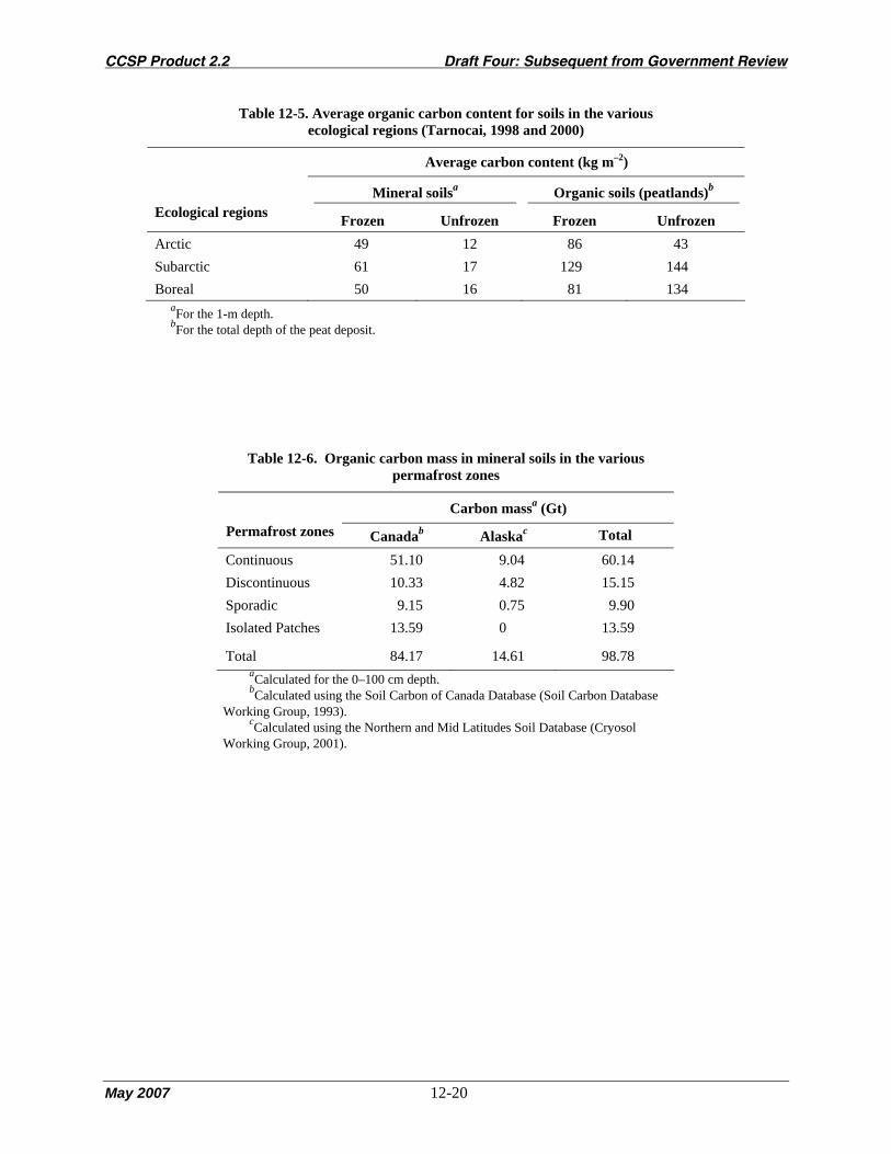
CCSP Product 2.2 Draft Four: Subsequent from Government Review
May 2007 12-20
Table 12-5. Average organic carbon content for soils in the various ecological regions (Tarnocai, 1998 and 2000)
Average carbon content (kg m–2)
Mineral soilsa Organic soils (peatlands)b
Ecological regions Frozen Unfrozen Frozen Unfrozen Arctic 49 12 86 43 Subarctic 61 17 129 144 Boreal 50 16 81 134
aFor the 1-m depth. bFor the total depth of the peat deposit.
Table 12-6. Organic carbon mass in mineral soils in the various permafrost zones
Carbon massa (Gt) Permafrost zones Canadab Alaskac Total
Continuous 51.10 9.04 60.14 Discontinuous 10.33 4.82 15.15 Sporadic 9.15 0.75 9.90 Isolated Patches 13.59 0 13.59
Total 84.17 14.61 98.78 aCalculated for the 0–100 cm depth. bCalculated using the Soil Carbon of Canada Database (Soil Carbon Database
Working Group, 1993). cCalculated using the Northern and Mid Latitudes Soil Database (Cryosol
Working Group, 2001).

CCSP Product 2.2 Draft Four: Subsequent from Government Review
May 2007 12-21
Table 12-7. Organic carbon mass in peatlands (organic soils) in the various permafrost zones
Carbon massa (Gt) Permafrost zones Canadab Alaskac Total
Continuous 21.82 1.46 23.28 Discontinuous 26.54 0.84 27.38 Sporadic 30.66 0.27 30.93 Isolated Patches 32.95 0 32.95
Total 111.97 2.57 114.54 aCalculated for the total depth of the peat deposit. bCalculated using the Peatlands of Canada Database (Tarnocai et al., 2005). cCalculated using the Northern and Mid Latitudes Soil Database (Cryosol
Working Group, 2001).
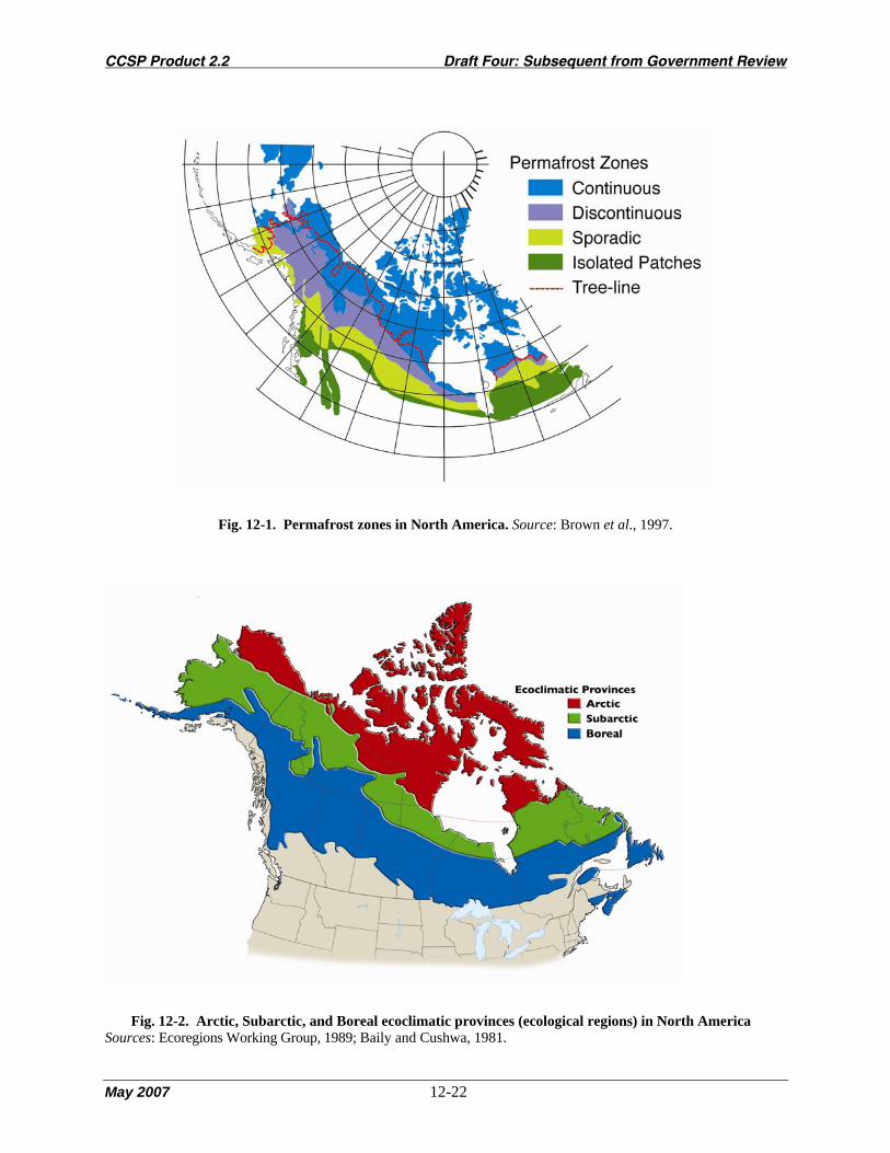
CCSP Product 2.2 Draft Four: Subsequent from Government Review
May 2007 12-22
Fig. 12-1. Permafrost zones in North America. Source: Brown et al., 1997.
Fig. 12-2. Arctic, Subarctic, and Boreal ecoclimatic provinces (ecological regions) in North America Sources: Ecoregions Working Group, 1989; Baily and Cushwa, 1981.

CCSP Product 2.2 Draft Four: Subsequent from Government Review
May 2007 12-23
Carbon sinks Carbon sources
Permafrost-affected soil with a thick surface organic layer, dark-colored organic intrusions in the brown soil layer, and an underlying frozen, high-ice-content layer. The organic intrusions were translocated from the surface by cryoturbation. (Mackenzie Valley, Canada)
Eroding high-ice-content permafrost soil composed of a dark frozen soil layer with an almost pure ice layer below. The thawing process generated a flow slide in which high-organic- content soil materials slumped into the water- saturated environment. (Mackenzie Delta area, Canada)
Perennially frozen deposit composed of an active layer that freezes and thaws annually and an underlying perennially frozen layer that has a high ice content. Organic material deposited annually on the soil surface builds up as an organic soil layer. Some of this surface organic material is translocated into the deeper soil layers by cryoturbation (1). In addition, soluble organic matter is translocated into the deeper soil layers by movement of water to the freezing front and by gravity (2). Because these deeper soil layers have low temperatures (0 to -15°C), the organic material decomposes very slowly. Thus more organic material accumulates as long as the soil is frozen. In this state, the permafrost soil acts as a carbon sink.
Thermal erosion initiated by climate warming, wildfires or human activity causes the high-ice-content mineral soils to thaw, releasing the organic materials locked in the system. In this environment aerobic (3) and anaerobic (4) decomposition occurs releasing carbon dioxide and methane. In this state, the soil is a source of carbon.
Fig. 12-3. Carbon cycle in permafrost-affected upland (mineral) soils, showing below-ground organic carbon sinks and sources.

CCSP Product 2.2 Draft Four: Subsequent from Government Review
May 2007 12-24
Carbon sinks Carbon sources
Perennially frozen peat deposit with multiple dark-colored peat layers. (Mackenzie River Delta area, Canada)
Eroding perennially frozen peat deposit, showing the large blocks of peat slumping into the water- saturated collapsed area. (Fort Simpson area, Canada)
Perennially frozen peat deposits consist of an active layer that freezes and thaws annually and an underlying perennially frozen layer composed of ice-rich frozen peat and mineral materials.
Organic material is deposited annually on the peatland surface. Although a large portion (>90%) of this organic material decomposes, the remainder is added to the peat deposit, producing an annual peat accumulation. The low soil temperatures (0 to –15°C) and the water-saturated and acid conditions cause this added organic carbon to be preserved and stored. This has been occurring for the last 5–8 thousand years. In this state, the peatland is a carbon sink.
Thermal erosion (thawing) of frozen peat deposits occurs as a result of climate change, wildfires, or human disturbances, releasing large amounts of water from the melting ice. This is mixed with the slumped peat material, initiating anaerobic decomposition in the much warmer environment. Anaerobic decomposition produces methane, which is expelled into the atmosphere. In this state, the peatland is a source of carbon.
Fig. 12-4. Carbon cycle in permafrost peatlands, showing below-ground organic carbon sinks and sources.

CCSP Product 2.2 Draft Four: Subsequent from Government Review
May 2007 12-25
Fig. 12-5. Carbon cycle in perennially frozen mineral soils in the permafrost region.
Fig. 12-6. Carbon cycle in peatlands in the permafrost region.

CCSP Product 2.2 Draft Four: Subsequent from Government Review
May 2007 12-26
0
5
10
15
20
25
30
35
40
45
No Change Very Slight Slight Moderate Severe ExtremelySevere
Sensitivity Class
Car
bon
Mas
s (G
t)
Subarctic Boreal Total
Fig. 12-7. The organic carbon mass in the various sensitivity classes for the Subarctic and Boreal Ecoclimatic Provinces (ecological regions). Source: Tarnocai, 2006.

CCSP Product 2.2 Draft Four: Subsequent from Government Review
May 2007 13-1
Chapter 13. Wetlands
Lead Author: Scott D. Bridgham1
Contributing Authors: J. Patrick Megonigal,2 Jason K. Keller,2 Norman B. Bliss3, and Carl Trettin4
1Center for Ecology and Evolutionary Biology, University of Oregon, 2Smithsonian Environmental Research Center,
3Science Applications International Corporation, USGS Center for Earth Resources Observation and Science, 4Center for Forested Wetland Research, USDA Forest Service
KEY FINDINGS
• North America is home to approximately 40% of the global wetland area, encompassing about 2.5
million square kilometers (965,000 square miles) with a carbon pool of approximately 223 billion tons,
mostly in peatland soils.
• North American wetlands currently are a carbon dioxide sink of approximately 49 million tons of
carbon per year, but that estimate has an uncertainty of greater than 100%. North American wetlands
are also a source of approximately 9 million tons of methane, a more potent atmospheric heat-
trapping gas. The uncertainty in that flux is also greater than 100%.
• Historically, the destruction of North American wetlands through land-use change has reduced carbon
storage in wetlands by 15 million tons of carbon per year, primarily through the oxidation of carbon in
peatland soils as they are drained and a more general reduction in carbon uptake and storage
capacity of wetlands converted to other land uses. Methane emissions have also declined with the
loss of wetland area.
• Projections of future carbon storage and methane emissions of North American wetlands are highly
uncertain and complex, but the large carbon pools in peatlands may be at risk for oxidation and
release to the atmosphere as carbon dioxide if they become substantially warmer and drier. Methane
emissions may increase with warming, but the response will likely vary with wetland type and with
changes in precipitation.
• Because of the potentially significant role of North American wetlands in methane production, the
activities associated with the restoration, creation and protection of wetlands are likely to focus on the
ecosystem services that wetlands provide, such as filtering of toxics, coastal erosion protection,
wildlife habitat, and havens of biological diversity, rather than on carbon sequestration, per se.

CCSP Product 2.2 Draft Four: Subsequent from Government Review
May 2007 13-2
• Research needs to reduce the uncertainties in carbon storage and fluxes in wetlands to provide
information about management options in terms of carbon uptake and storage and trace gas fluxes.
1. INTRODUCTION
While there are a variety of legal and scientific definitions of a wetland (National Research Council,
1995; National Wetlands Working Group, 1997), most emphasize the presence of waterlogged conditions
in the upper soil profile during at least part of the growing season, and plant species and soil conditions
that reflect these hydrologic conditions. Waterlogging tends to suppress microbial decomposition more
than plant productivity, so wetlands are known for their ability to accumulate large amounts of soil
carbon, most spectacularly seen in large peat deposits that are often many meters deep. Thus, when
examining carbon dynamics, it is important to distinguish between freshwater wetlands with surface soil
organic matter deposits greater than 40 cm thick (i.e., peatlands) and those with lesser amounts of soil
organic matter (i.e., freshwater mineral-soil wetlands, FWMS). Some wetlands have permafrost; fluxes
and pools in wetlands with and without permafrost are discussed separately in Appendix 13A. We also
differentiate between freshwater wetlands and estuarine wetlands (salt marshes, mangroves, and mud
flats) with marine-derived salinity.
Peatlands occupy about 3% of the terrestrial global surface, yet they contain 16–33% of the total soil
carbon pool (Gorham, 1991; Maltby and Immirzi, 1993). Most peatlands occur between 50 and 70º N,
although significant areas occur at lower latitudes (Matthews and Fung, 1987; Aselmann and Crutzen,
1989; Maltby and Immirzi, 1993). Large areas of peatlands exist in Alaska, Canada, and in the northern
midwestern, northeastern, and southeastern United States (Bridgham et al., 2000). Because this peat
formed over thousands of years, these areas represent a large carbon pool but with relatively slow rates of
accumulation. By comparison, estuarine wetlands and some freshwater mineral-soil wetlands rapidly
sequester carbon as soil organic matter due to rapid burial in sediments. Large areas of wetlands have
been converted to other land uses globally and in North America (Dugan, 1993; OECD, 1996), which
may have resulted in a net flux of carbon to the atmosphere (Armentano and Menges, 1986; Maltby and
Immirzi, 1993). Additionally, wetlands emit 92–237 million tons of methane (Mt CH4) per year,† which is
a large fraction of the total annual global flux of about 600 Mt CH4 per year (Ehhalt et al., 2001).† This is
important because methane is a potent greenhouse gas, second in importance to only carbon dioxide
(Ehhalt et al., 2001).
† The uncertainties for the numerical values cited in this chapter are presented and explained in Table 13-1.

CCSP Product 2.2 Draft Four: Subsequent from Government Review
May 2007 13-3
A number of previous studies have examined the role of peatlands in the global carbon balance
(reviewed in Mitra et al., 2005), and Roulet (2000) focused on the role of Canadian peatlands in the
Kyoto process. Here we augment these previous studies by considering all types of wetlands (not just
peatlands) and integrate new data to examine the carbon balance in the wetlands of Canada, the United
States, and Mexico. We also briefly compare these values to those from global wetlands. We limit this
review to those components of the carbon budget that result in a net gaseous exchange with the
atmosphere on an interannual basis and do not consider other internal carbon fluxes. We do not consider
dissolved organic carbon (DOC) fluxes from wetlands, although they may be substantial (Moore 1997),
because the oxidation of the DOC would be counted as atmospheric carbon emissions in the receiving
ecosystems downstream, and we do not want to double-count fluxes.
Given that many undisturbed wetlands are a natural sink for carbon dioxide and a source of methane,
a note of caution in interpretation of our data is important. Using the International Panel on Climate
Change (IPCC) terminology, a radiative forcing denotes “an externally imposed perturbation in the
radiative energy budget of the Earth’s climate system” (Ramaswamy et al., 2001). Thus, it is the change
from a baseline condition in greenhouse gas fluxes in wetlands that constitute a radiative forcing that will
impact climate change, and carbon fluxes in unperturbed wetlands are important only in establishing a
baseline condition. For example, historical steady state rates of methane emissions from wetlands have
zero net radiative forcing, but an increase in methane emissions due to climatic warming would constitute
a positive radiative forcing. Similarly, steady state rates of soil carbon sequestration in wetlands have zero
net radiative forcing, but the lost sequestration capacity and the oxidation of the soil carbon pool in
drained wetlands are both positive radiative forcings.
2. INVENTORIES
2.1 Current Wetland Area and Rates of Loss
The current and original wetland area and rates of loss are the basis for all further estimates of pools
and fluxes in this chapter. The loss of wetlands has caused the oxidation of their soil carbon, particularly
in peatlands, reduced their ability to sequester carbon, and reduced their emissions of methane. The
strengths and weakness of the wetland inventories of Canada, the United States, and Mexico are discussed
in Appendix 13A.
The conterminous United States has 312,000 km2 of FWMS wetlands, 93,000 km2 of peatlands, and
25,000 km2 of estuarine wetlands, which encompass 5.5% of the land area (Table 13-1). This represents
just 48% of the original wetland area in the conterminous United States (Table 13A-1 in Appendix 13A).
However, wetland losses in the United States have declined from 1,855 km2 yr–1 in the 1950s–1970s to
237 km2 yr–1 in the 1980s–1990s (Dahl, 2000). Such data mask large differences in loss rates among

CCSP Product 2.2 Draft Four: Subsequent from Government Review
May 2007 13-4
wetland classes and conversion of wetlands to other classes (Dahl, 2000), with potentially large effects on
carbon stocks and fluxes. For example, the majority of wetland losses in the United States have occurred
in FWMS wetlands. As of the early 1980s, 84% of U.S. peatlands were unaltered (Armentano and
Menges, 1986; Maltby and Immirzi, 1993; Rubec, 1996), and, given the current regulatory environment
in the United States, recent rates of loss are likely small.
Table 13-1. The area, carbon pool, net carbon balance, and methane flux from wetlands in North
America and the world.
Canada has 1,301,000 km2 of wetlands, covering 14% of its land area, of which 87% are peatlands
(Table 13-1). Canada has lost about 14% of its wetlands, mainly due to agricultural development of
FWMS wetlands (Rubec, 1996), although the ability to estimate wetland losses in Canada is limited by
the lack of a regular wetland inventory.
The wetland area in Mexico is estimated at 36,000 km2 (Table 13-1), with an estimated historical loss
of 16,000 km2 (Table 13A-1 in Appendix 13A). However, given the lack of a nationwide wetland
inventory and a general paucity of data, this number is highly uncertain.
Problems with inadequate wetland inventories are even more prevalent in lesser developed countries
(Finlayson et al., 1999). We estimate a global wetland area of 6.0 × 10⁶ km2 (Table 13-1); thus, North
America currently has about 43% of the global wetland area. It has been estimated that about 50% of the
world’s original wetlands have been converted to other uses (Moser et al., 1996).
2.2 Carbon Pools
We estimate that North American wetlands have a current soil and plant carbon pool of 223 billion
tons (Gt), of which approximately 98% is in the soil (Table 13-1). The majority of this carbon is in
peatlands, with FWMS wetlands contributing about 18% of the carbon pool. The large amount of soil
carbon (27 Gt) in Alaskan FWMS wetlands had not been identified in previous studies (see Appendix
13A).
2.3 Soil Carbon Fluxes
North American peatlands currently have a net carbon balance of about -17 million tons of carbon
(Mt C) per year (Table 13-1), but several large fluxes are incorporated into this estimate. (Negative
numbers indicate net fluxes into the ecosystem, whereas positive numbers indicate next fluxes into
the atmosphere.) Peatlands sequester -29 Mt C per year (Table 13A-2 in Appendix 13A). However, this
carbon sink is partially offset by a net oxidative flux of 18 Mt C per year as of the early 1980s in
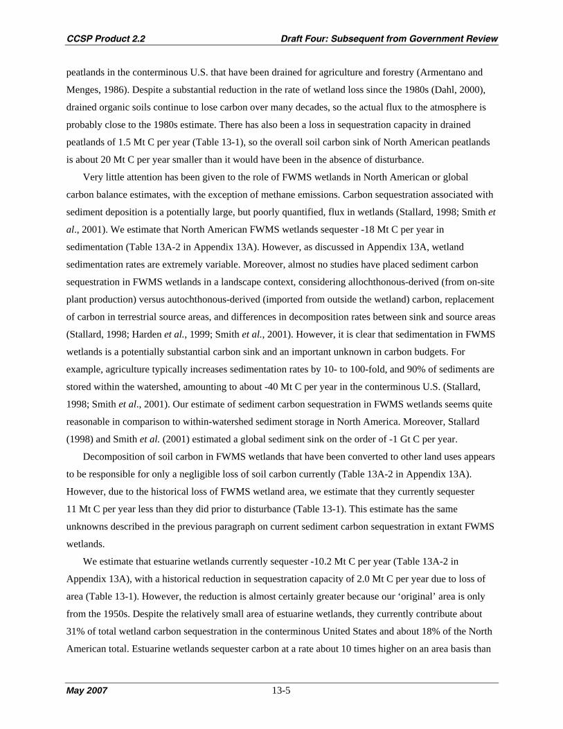
CCSP Product 2.2 Draft Four: Subsequent from Government Review
May 2007 13-5
peatlands in the conterminous U.S. that have been drained for agriculture and forestry (Armentano and
Menges, 1986). Despite a substantial reduction in the rate of wetland loss since the 1980s (Dahl, 2000),
drained organic soils continue to lose carbon over many decades, so the actual flux to the atmosphere is
probably close to the 1980s estimate. There has also been a loss in sequestration capacity in drained
peatlands of 1.5 Mt C per year (Table 13-1), so the overall soil carbon sink of North American peatlands
is about 20 Mt C per year smaller than it would have been in the absence of disturbance.
Very little attention has been given to the role of FWMS wetlands in North American or global
carbon balance estimates, with the exception of methane emissions. Carbon sequestration associated with
sediment deposition is a potentially large, but poorly quantified, flux in wetlands (Stallard, 1998; Smith et
al., 2001). We estimate that North American FWMS wetlands sequester -18 Mt C per year in
sedimentation (Table 13A-2 in Appendix 13A). However, as discussed in Appendix 13A, wetland
sedimentation rates are extremely variable. Moreover, almost no studies have placed sediment carbon
sequestration in FWMS wetlands in a landscape context, considering allochthonous-derived (from on-site
plant production) versus autochthonous-derived (imported from outside the wetland) carbon, replacement
of carbon in terrestrial source areas, and differences in decomposition rates between sink and source areas
(Stallard, 1998; Harden et al., 1999; Smith et al., 2001). However, it is clear that sedimentation in FWMS
wetlands is a potentially substantial carbon sink and an important unknown in carbon budgets. For
example, agriculture typically increases sedimentation rates by 10- to 100-fold, and 90% of sediments are
stored within the watershed, amounting to about -40 Mt C per year in the conterminous U.S. (Stallard,
1998; Smith et al., 2001). Our estimate of sediment carbon sequestration in FWMS wetlands seems quite
reasonable in comparison to within-watershed sediment storage in North America. Moreover, Stallard
(1998) and Smith et al. (2001) estimated a global sediment sink on the order of -1 Gt C per year.
Decomposition of soil carbon in FWMS wetlands that have been converted to other land uses appears
to be responsible for only a negligible loss of soil carbon currently (Table 13A-2 in Appendix 13A).
However, due to the historical loss of FWMS wetland area, we estimate that they currently sequester
11 Mt C per year less than they did prior to disturbance (Table 13-1). This estimate has the same
unknowns described in the previous paragraph on current sediment carbon sequestration in extant FWMS
wetlands.
We estimate that estuarine wetlands currently sequester -10.2 Mt C per year (Table 13A-2 in
Appendix 13A), with a historical reduction in sequestration capacity of 2.0 Mt C per year due to loss of
area (Table 13-1). However, the reduction is almost certainly greater because our ‘original’ area is only
from the 1950s. Despite the relatively small area of estuarine wetlands, they currently contribute about
31% of total wetland carbon sequestration in the conterminous United States and about 18% of the North
American total. Estuarine wetlands sequester carbon at a rate about 10 times higher on an area basis than

CCSP Product 2.2 Draft Four: Subsequent from Government Review
May 2007 13-6
other wetland ecosystems due to high sedimentation rates, high soil carbon content, and constant burial
due to sea level rise. Estimates of sediment deposition rates in estuarine wetlands are reasonably robust,
but the same ‘landscape’ issues of allochthonous versus autochthonous inputs of carbon, replenishment of
carbon in source area soils, and differences in decomposition rates between sink and source areas exist as
for FWMS wetlands. Another large uncertainty in the estuarine carbon budget is the area and carbon
content of mud flats, particularly in Canada and Mexico.
Overall, North American wetland soils appear to be a substantial carbon sink with a net flux of
-49 Mt C per year (with very large error bounds because of FWMS wetlands) (Table 13-1). The large-
scale conversion of wetlands to upland uses has led to a reduction in the wetland soil carbon sequestration
capacity of 15 Mt C per year from the likely historical rate (Table 13-1), but this estimate is driven by
large losses of FWMS wetlands with their highly uncertain sedimentation carbon sink. Adding in the
current net oxidative flux of 18 Mt C per year from conterminous U.S. peatlands, we estimate that North
American wetlands currently sequester 33 Mt C per year less than they did historically (Table 13A-2 in
Appendix 13A). Furthermore, North American peatlands and FWMS wetlands have lost 2.6 Gt and 0.8 Gt
of soil carbon, respectively, and collectively they have lost 2.4 Gt of plant carbon since approximately
1800. Very little data exist to estimate carbon fluxes for freshwater Mexican wetlands, but because of
their small area, they will not likely have a large impact on the overall North American estimates.
The global wetland soil carbon balance has only been examined in peatlands, which currently are a
moderate source of atmospheric carbon of about 150 Mt C per year (Table 13-1), largely due to the
oxidation of peat drained for agriculture and forestry and secondarily due to peat combustion for fuel
(Armentano and Menges, 1986; Maltby and Immirzi, 1993). The cumulative historical shift in soil carbon
stocks has been estimated to be 5.5 to 7.1 Gt C (Maltby and Immirzi, 1993). Although we are aware of no
previous evaluation of the carbon balance of global FWMS and estuarine wetlands, using the assumption
noted above, we estimate that they are a sink of approximately -39 and -43 Mt per year, respectively.
2.4 Methane and Nitrous Oxide Emissions
We estimate that North American wetlands emit 9.4 Mt CH4 per year (Table 13-1). For comparison, a
mechanistic methane model yielded emissions of 3.8 and 7.1 Mt CH4 per year for Alaska and Canada,
respectively (Zhuang et al., 2004). A regional inverse atmospheric modeling approach estimated total
methane emissions (from all sources) of 16 and 54 Mt CH4 per year for boreal and temperate North
America, respectively (Fletcher et al., 2004b).
Methane emissions are currently about 5 Mt CH4 per year less than they were historically in North
American wetlands (see Table 13A-4 in Appendix 13A) because of the loss of wetland area. We do not
consider the effects of conversion of wetlands from one type to another (Dahl, 2000), which may have a

CCSP Product 2.2 Draft Four: Subsequent from Government Review
May 2007 13-7
significant impact on methane emissions. Similarly, we estimate that global methane emissions from
natural wetlands are only about half of what they were historically due to loss of area (Table 13A-4 in
Appendix 13A). However, this may be an overestimate because wetland losses have been higher in more
developed countries than less developed countries (Moser et al., 1996), and wetlands at lower latitudes
have higher emissions on average (Bartlett and Harriss, 1993).
When we multiplied the very low published estimates of nitrous oxide emissions from natural and
disturbed wetlands (Joosten and Clarke, 2002) by North American wetland area, the flux was insignificant
(data not shown). However, nitrous oxide emissions have been measured in few wetlands, particularly in
FWMS wetlands and wetlands with high nitrogen inputs (e.g., from agricultural run-off), where emissions
might be expected to be higher.
We use global warming potentials (GWPs) as a convenient way to compare the relative contributions
of carbon dioxide and methane fluxes in North American wetlands to the Earth’s radiative balance. The
GWP is the radiative effect of a pulse of a substance into the atmosphere relative to carbon dioxide over a
particular time horizon (Ramaswamy et al., 2001). However, it is important to distinguish between
radiative balance, which refers to the static radiative effect of a substance, and radiative forcing which
refers to an externally imposed perturbation on the Earth’s radiative energy budget (Ramaswamy et al.,
2001). Thus, changes in radiative balance lead to a radiative forcing, which subsequently leads to a
change in the Earth’s surface temperature. For example, wetlands have a large effect on the Earth’s
radiative balance through high methane emissions, but, it is only to the extent that emissions change
through time that they represent a positive or negative radiative forcing and impact climate change.
Methane has GWPs of 1.9, 6.3, and 16.9 CO2-carbon equivalents on a mass basis across 500-year,
100-year, and 20-year time frames, respectively (Ramaswamy et al., 2001)1. Depending upon the time
frame and within the large confidence limits of many of our estimates in Table 13-1, the net radiative
balance of North American wetlands as a whole currently are approximately neutral in terms of net CO2-
carbon equivalents to the atmosphere (note that we discuss net radiative forcing in Trends and Drivers of
Wetland Carbon Fluxes). The exception is estuarine wetlands, which are a net sink for CO2-carbon
equivalents because they support both rapid rates of carbon sequestration and low methane emissions.
However, caution should be exercised in using GWPs to draw conclusions about changes in the net flux
of CO2-carbon equivalents because GWPs are based upon a pulse of a gas into the atmosphere, whereas
carbon sequestration is more or less continuous. For example, if one considers continuous methane
emissions and carbon sequestration in peat over time, most peatlands are a net sink for CO2-carbon
equivalents because of the long lifetime of carbon dioxide sequestered as peat (Frolking et al., 2006).
1GWPs in Ramaswamy et al. (2001) were originally reported in CO2-mass equivalents. We have converted them into CO2-carbon equivalents so that the net carbon balance and methane flux columns in Table 13-1 can be directly compared by multiplying methane fluxes by the GWPs given here.

CCSP Product 2.2 Draft Four: Subsequent from Government Review
May 2007 13-8
2.5 Plant Carbon Fluxes
We estimate that wetland forests in the conterminous United States currently sequester -10.3 Mt C
per year as increased plant biomass (see Table 13A-3 in Appendix 13A). Sequestration in plants in
undisturbed wetland forests in Alaska, many peatlands, and estuarine wetlands is probably minimal,
although there may be substantial logging of Canadian forested peatlands that we do not have the data to
account for.
3. TRENDS AND DRIVERS OF WETLAND CARBON FLUXES
While extensive research has been done on carbon cycling and pools in North American wetlands, to
our knowledge, this is the first attempt at an overall carbon budget for all of the wetlands of North
America, although others have examined the carbon budget for North American peatlands as part of
global assessments (Armentano and Menges, 1986; Maltby and Immirzi, 1993; Joosten and Clarke,
2002). Historically, the destruction of wetlands through land-use changes has had the largest effect on the
carbon fluxes and, consequently, the radiative forcing of North American wetlands. The primary effects
have been a reduction in their ability to sequester carbon (a small to moderate increase in radiative forcing
depending on carbon sequestration by sedimentation in FWMS and estuarine wetlands), oxidation of their
soil carbon reserves upon drainage (a small increase in radiative forcing), and a reduction in methane
emissions (a small to large decrease in radiative forcing depending on actual emissions) (Table 13A-1 and
Appendix 13A). Globally, the disturbance of peatlands appears to have shifted them into a net source of
carbon to the atmosphere. Any positive effect of wetland loss due to a reduction in their methane
emissions, and hence radiative forcing, will be more than negated by the loss of the many ecosystem
services they provide such as havens for biodiversity, recharge of groundwater, reduction in flooding, fish
nurseries, etc. (Zedler and Kercher, 2005).
A majority of the effort in examining future global change impacts on wetlands has focused on
northern peatlands because of their large soil carbon reserves, although under current climate conditions
they have modest methane emissions (Moore and Roulet, 1995; Roulet, 2000; Joosten and Clarke, 2002,
and references therein). The effects of global change on carbon sequestration in peatlands are probably of
minor importance as a global flux because of the relatively low rate of peat accumulation. However,
losses of soil carbon stocks in peatlands drained for agriculture and forestry (Table 13A-2 in Appendix
13A) attest to the possibility of large losses from the massive soil carbon deposits in northern peatlands if
they become substantially drier in a future climate. Furthermore, Turetsky et al. (2004) estimated that up
to 5.9 Mt C per year are released from western Canadian peatlands by fire and predicted that increases in
fire frequency may cause these systems to become net atmospheric carbon sources. We did not add this
flux to our estimate of the net carbon balance of North American wetlands because historical oxidation of

CCSP Product 2.2 Draft Four: Subsequent from Government Review
May 2007 13-9
peat by fire should be integrated in the peat sequestration estimates and recent changes due to
anthropogenic effects are highly uncertain.
Our compilation shows that attention needs to be directed toward understanding climate change
impacts to FWMS wetlands, which collectively emit similar amounts of methane and potentially
sequester an equivalent amount of carbon than peatlands. The effects of changing water table depths are
somewhat more tractable in FWMS wetlands than peatlands because FWMS wetlands have less potential
for oxidation of soil organic matter. In forested FWMS wetlands, increased precipitation and runoff may
increase radiative forcing by simultaneously decreasing wood production and increasing methanogenesis
(Megonigal et al., 2005). The influence of changes in hydrology on methane emissions, plant
productivity, soil carbon preservation, and sedimentation will need to be addressed in order to fully
anticipate climate change impacts on radiative forcing in these systems.
The effects of global change on estuarine wetlands is of concern because sequestration rates are rapid,
and they can be expected to increase in proportion to the rate of sea level rise provided estuarine wetland
area does not decline. Because methane emissions from estuarine wetlands are low, this increase in
sequestration capacity could represent a net decrease in radiative forcing, depending on how much of the
sequestered carbon is autochthonous. Changes in tidal wetland area with sea-level rise will depend on
rates of inland migration, erosion at the wetland-estuary boundary, and wetland elevation change. The
rate of loss of tidal wetland area has declined in past decades due to regulations on draining and filling
activities (Dahl, 2000). However, rapid conversion to open water is occurring in coastal Louisiana
(Bourne, 2000) and Maryland (Kearney and Stevenson, 1991), suggesting that marsh area will decline
with increased rates of sea level rise (Kearney et al., 2002). A multitude of human and climate factors are
contributing to the current losses (Turner, 1997; Day Jr. et al., 2000; Day Jr. et al., 2001). Although it is
uncertain how global changes in climate, eutrophication, and other factors will interact with sea level rise
(Najjar et al., 2000), it is likely that increased rates of sea level rise will cause an overall decline in
estuarine marsh area and soil carbon sequestration.
One of the greatest concerns is how climate change will affect future methane emissions from
wetlands because of their large GWP. Wetlands emit about 105 Mt CH4 per year (Table 13-1), or 20% of
the global total. Increases in atmospheric methane concentrations over the past century have had the
second largest radiative forcing (after carbon dioxide) in human-induced climate change (Ehhalt et al.,
2001). Moreover, methane fluxes from wetlands have provided an important radiative feedback on
climate over the geologic past (Chappellaz et al., 1993; Blunier et al., 1995; Petit et al., 1999). The large
global warming observed since the 1990s may have resulted in increased methane emissions from
wetlands (Fletcher et al., 2004a; Wang et al., 2004; Zhuang et al., 2004).

CCSP Product 2.2 Draft Four: Subsequent from Government Review
May 2007 13-10
Data (Bartlett and Harriss, 1993; Moore et al., 1998; Updegraff et al., 2001) and modeling (Gedney et
al., 2004; Zhuang et al., 2004) strongly support the contention that water table position and temperature
are the primary environmental controls over methane emissions. How this generalization plays out with
future climate change is, however, more complex. For example, most climate models predict much of
Canada will be warmer and drier in the future. Based upon this prediction, Moore et al. (1998) proposed a
variety of responses to climate change in the carbon fluxes from different types of Canadian peatlands.
Methane emissions may increase in collapsed former-permafrost bogs (which will be warmer and wetter)
but decrease in fens and other types of bogs (warmer and drier). A methane-process model predicted that
modest warming will increase global wetland emissions, but larger increases in temperature will decrease
emissions because of drier conditions (Cao et al., 1998).
The direct, non-climatic effects of increasing atmospheric carbon dioxide on carbon cycling in
wetland ecosystems has received far less attention than upland systems. Field studies have been done in
tussock tundra (Tissue and Oechel, 1987; Oechel et al. 1994), bog-type peatlands (Hoosbeek et al., 2001),
rice paddies (Kim et al., 2001), and a salt marsh (Rasse et al., 2005); and a somewhat wider variety of
wetlands have been studied in small scale glasshouse systems. Temperate and tropical wetland
ecosystems consistently respond to elevated carbon dioxide with an increase in photosynthesis and/or
biomass (Vann and Megonigal, 2003). By comparison, the response of northern peatland plant
communities has been inconsistent. A hypothesis that remains untested is that the elevated carbon dioxide
response of northern peatlands will be limited by nitrogen availability. In an in situ study of tussock
tundra, complete photosynthetic acclimation occurred when carbon dioxide was elevated, but acclimation
was far less severe with both elevated carbon dioxide and a 4oC increase in air temperature (Oechel et al.,
1994). It was hypothesized that soil warming relieved a severe nutrient limitation on photosynthesis by
increasing nitrogen mineralization.
A consistent response to elevated carbon dioxide-enhanced photosynthesis in wetlands is an
increase in methane emissions ranging from 50 to 350% (Megonigal and Schlesinger, 1997; Vann and
Megonigal, 2003). It is generally assumed that the increased supply of plant photosynthate stimulates
anaerobic microbial carbon metabolism, of which methane is a primary end product. An increase in
methane emissions from wetlands due to elevated carbon dioxide constitutes a positive feedback on
radiative forcing because carbon dioxide is rapidly converted to a more effective greenhouse gas
(methane).
An elevated carbon dioxide-induced increase in methane emissions may be offset by an increase
in carbon sequestration in soil organic matter or wood. Although there are very little data to evaluate this
hypothesis, a study on seedlings of a wetland-adapted tree species reported that elevated carbon dioxide
stimulated photosynthesis and methane emissions, but not growth, under flooded conditions (Megonigal

CCSP Product 2.2 Draft Four: Subsequent from Government Review
May 2007 13-11
et al., 2005). It is possible that elevated carbon dioxide will stimulate soil carbon sequestration,
particularly in tidal wetlands experiencing sea level rise, but a net loss of soil carbon is also possible due
to priming effects (i.e., increased labile carbon inputs from elevated carbon dioxide enhance
decomposition of the overall soil carbon pool) (Hoosbeek et al., 2004; Lichter et al., 2005). Elevated
carbon dioxide has the potential to influence the carbon budgets of adjacent aquatic ecosystems by
increasing export of dissolved organic carbon (Freeman et al., 2004) and dissolved inorganic carbon
(Marsh et al., 2005).
Other important anthropogenic forcing factors that will affect future methane emissions include
atmospheric sulfate deposition (Vile et al., 2003; Gauci et al., 2004) and nutrient additions (Keller et al.,
2005). These external forcing factors in turn will interact with internal ecosystem constraints such as pH
and carbon quality (Moore and Roulet, 1995; Bridgham et al., 1998), anaerobic carbon flow (Hines and
Duddleston, 2001), and net ecosystem productivity and plant community composition (Whiting and
Chanton, 1993; Updegraff et al., 2001; Strack et al., 2004) to determine the actual response.
4. OPTIONS FOR MANAGEMENT
Wetland policies in the United States and Canada are driven by a variety of federal, state or
provincial, and local laws and regulations in recognition of the many wetland ecosystem services and
large historical loss rates (Lynch-Stewart et al., 1999; National Research Council, 2001; Zedler and
Kercher, 2005). Thus, any actions to enhance the ability of wetlands to sequester carbon, or reduce their
methane emissions, must be implemented within the context of the existing regulatory framework. The
most important option in the United States has already been largely achieved, and that is to reduce the
historical rate of peatland losses with their accompanying large oxidative losses of the stored soil carbon.
Decreases in the rates of loss of all wetlands have helped to maintain their soil carbon sequestration
potential.
There has been strong interest expressed in using carbon sequestration as a rationale for wetland
restoration and creation in the United States, Canada, and elsewhere (Wylynko, 1999; Watson et al.,
2000). However, high methane emissions from conterminous U.S. wetlands suggest that creating and
restoring wetlands may increase net radiative forcing, although adequate data do not exist to fully
evaluate this possibility. Roulet (2000) came to a similar conclusion concerning the restoration of
Canadian wetlands. Net radiative forcing from restoration will likely vary among different kinds of
wetlands and the specifics of their carbon budgets. The possibility of increasing radiative forcing by
creating or restoring wetlands does not apply to estuarine wetlands, which emit relatively little methane
compared to the carbon they sequester. Restoration of drained peatlands may stop the rapid loss of their
soil carbon, which may compensate for increased methane emissions. However, Canadian peatlands

CCSP Product 2.2 Draft Four: Subsequent from Government Review
May 2007 13-12
restored from peat extraction operations increased their net emissions of carbon because of straw addition
during the restoration process, although it was assumed that they would eventually become a net sink
(Cleary et al., 2005).
Regardless of their internal carbon balance, the area of restored wetlands is currently too small to
form a significant carbon sink at the continental scale. Between 1986 and 1997, only 4,157 km2 of
uplands were converted into wetlands in the conterminous United States (Dahl, 2000). Using the soil
carbon sequestration rate of 3.05 Mg C ha-1 yr-1 found by Euliss et al. (2006) for restored prairie pothole
wetlands2, we estimate that wetland restoration in the U.S. would have sequestered 1.3 Mt C over this 11-
year period. However, larger areas of wetland restoration may have a significant impact on carbon
sequestration. A simulation model of planting 20,000 km2 into bottomland hardwood trees as part of the
Wetland Reserve Program in the United States showed a sequestration of 4 Mt C per year through 2045
(Barker et al., 1996). Euliss et al. (2006) estimated that if all cropland on former prairie pothole wetlands
in the U.S. and Canada (162,244 km2) were restored that 378 Mt C would be sequestered over 10 years in
soils and plants. However, neither study accounted for the GWP of increased methane emissions.
Potentially more significant is the conversion of wetlands from one type to another; for example,
8.7% (37,200 km2) of the wetlands in the conterminous United States in 1997 were in a previous wetland
category in 1986 (Dahl, 2000). The net effect of these conversions on wetland carbon fluxes is unknown.
Similarly, Roulet (2000) argued that too many uncertainties exist to include Canadian wetlands in the
Kyoto Protocol.
In summary, North American wetlands form a very large carbon pool, primarily because of storage as
peat, and are a small-to-moderate carbon sink (excluding methane effects). The largest unknown in the
wetland carbon budget is the amount and significance of sedimentation in FWMS and estuarine wetlands
and methane emissions in freshwater wetlands. With the exception of estuarine wetlands, methane
emissions from wetlands may largely offset any positive benefits of carbon sequestration in soils and
plants. Given these conclusions, it is probably unwarranted to use carbon sequestration as a rationale for
the protection and restoration of FWMS wetlands, although the many other ecosystem services that they
provide justify these actions. However, protecting and restoring peatlands will stop the loss of their soil
carbon (at least over the long term), and estuarine wetlands are an important carbon sink given their
limited areal extent and low methane emissions.
The most important areas for further scientific research in terms of current carbon fluxes in the United
States are to establish an unbiased, landscape-level sampling scheme to determine sediment carbon
sequestration in FWMS and estuarine wetlands and additional measurements of annual methane
2Euliss et al. (2006) regressed surface soil carbon stores in 27 restored semi-permanent prairie pothole wetlands against years since restoration to derive this estimate (r2 = 0.31, P = 0.002). However, there was no significant relationship in seasonal prairie pothole wetlands (r2 = 0.04, P = 0.241).

CCSP Product 2.2 Draft Four: Subsequent from Government Review
May 2007 13-13
emissions to better constrain these important fluxes. It would also be beneficial if the approximately
decadal National Wetland Inventory (NWI) status and trends data were collected in sufficient detail with
respect to the Cowardin et al. (1979) classification scheme to determine changes among mineral-soil
wetlands and peatlands.
Canada lacks any regular inventory of its wetlands, and thus it is difficult to quantify land-use impacts
upon their carbon fluxes and pools. While excellent scientific data exists on most aspects of carbon
cycling in Canadian peatlands, Canadian FWMS and estuarine wetlands have been relatively poorly
studied, despite having suffered large proportional losses to land-use change. Wetland data for Mexico is
almost entirely lacking. Thus, anything that can be done to improve upon this would be helpful. All
wetland inventories should consider the area of estuarine mud flats, which have the potential to sequester
considerable carbon, and are poorly understood with respect to carbon sequestration.
The greatest unknown is how global change will affect the carbon pools and fluxes of North
American wetlands. We will not be able to accurately predict the role of North American wetlands as
potential positive or negative feedbacks to anthropogenic climate change without knowing the integrative
effects of changes in temperature, precipitation, atmospheric carbon dioxide concentrations, and
atmospheric deposition of nitrogen and sulfur within the context of internal ecosystem drivers of
wetlands. To our knowledge, no manipulative experiment has simultaneously measured more than two of
these perturbations in any North American wetland, and few have been done at any site. Modeling
expertise of the carbon dynamics of wetlands has rapidly improved in the last few years (Frolking et al.,
2002; Zhuang et al., 2004, and references therein), but this needs even further development in the future,
including for FWMS and estuarine wetlands.
ACKNOWLEDGMENTS
Steve Campbell [U.S. Department of Agriculture (USDA) National Resource Conservation Service
(NRCS), OR] synthesized the National Soil Information database so that it was useful to us. Information
on wetland soils within specific states was provided by Joseph Moore (USDA NRCS, AK), Robert
Weihrouch (USDA NRCS, WI), and Susan Platz (USDA NRCS, MN). Charles Tarnocai provided
invaluable data on Canadian peatlands. Thomas Dahl (U.S. Fish and Wildlife Service) explored the
possibility of combining NWI data with U.S. soils maps. Nigel Roulet (McGill University) gave valuable
advice on recent references. R. Kelman Wieder provided useful initial information on peatlands in
Canada. Comments of two anonymous reviewers and Shuguang Liu (USGS Center for Earth Resources
Observation and Science) greatly improved this manuscript.

CCSP Product 2.2 Draft Four: Subsequent from Government Review
May 2007 13-14
CHAPTER 13 REFERENCES
Armentano, T.B. and E.S. Menges, 1986: Patterns of change in the carbon balance of organic soil-wetlands of the
temperate zone. Journal of Ecology, 74, 755–774.
Aselmann, I. and P.J. Crutzen, 1989: Global distribution of natural freshwater wetlands and rice paddies, their net
primary productivity, seasonality and possible methane emissions. Journal of Atmospheric Chemistry, 8, 307–
359.
Barker, J.R., G.A. Baumgardner, D.P. Turner, and J.J. Lee, 1996: Carbon dynamics of the conservation and wetland
reserve program. Journal of Soil and Water Conservation, 51, 340–346.
Bartlett, K.B. and R.C. Harriss, 1993: Review and assessment of methane emissions from wetlands. Chemosphere,
26, 261–320.
Blunier, T., J. Chappellaz, J. Schwander, B. Stauffer, and D. Raynaud, 1995: Variations in atmospheric methane
concentration during the Holocene epoch. Nature, 374, 46–49.
Bourne, J., 2000: Louisiana's vanishing wetlands: going, going…. Science, 289, 1860–1863.
Bridgham, S.D., C.-L. Ping, J.L. Richardson, and K. Updegraff, 2000: Soils of northern peatlands: Histosols and
Gelisols. In: Wetland Soils: Genesis, Hydrology, Landscapes, and Classification [Richardson, J.L. and M.J.
Vepraskas (eds.)]. CRC Press, Boca Raton, FL, pp. 343–370.
Bridgham, S.D., K. Updegraff, and J. Pastor, 1998: Carbon, nitrogen, and phosphorus mineralization in northern
wetlands. Ecology, 79, 1545–1561.
Cao, M., K. Gregson, and S. Marshall, 1998: Global methane emission from wetlands and its sensitivity to climate
change. Atmospheric Environment, 32, 3293–3299.
Chappellaz, J., T. Bluniert, D. Raynaud, J.M. Barnola, J. Schwander, and B. Stauffert, 1993: Synchronous changes
in atmospheric CH4 and Greenland climate between 40 and 8 kyr B.P. Nature, 366, 443–445.
Cleary, J., N.T. Roulet, and T.R. Moore, 2005: Greenhouse gas emissions from Canadian peat extraction, 1990–
2000: a life-cycle analysis. Ambio, 34, 456–461.
Cowardin, L.M., V. Carter, F.C. Golet, and E.T. LaRoe, 1979: Classification of Wetlands and Deepwater Babitats
of the United States. FWS/OBS-79/31, Fish and Wildlife Service, U.S. Department of the Interior, Washington,
DC.
Dahl, T.E., 2000: Status and Trends of Wetlands in the Conterminous United States, 1986 to 1997. U.S. Department
of the Interior, Fish and Wildlife Service, Washington, DC.
Day Jr., J.W., G.P. Shafer, L.D. Britsch, D.J. Reed, S.R. Hawes, and D. Cahoon, 2000: Pattern and process of land
loss in the Mississippi Delta: a spatial and temporal analysis of wetland habitat change. Estuaries, 23, 425–438.
Day Jr., J.W., G.P. Shaffer, D.J. Reed, D.R. Cahoon, L.D. Britsch, and S.R. Hawes, 2001: Patterns and processes of
wetland loss in coastal Louisiana are complex: a reply to Turner 2001. estimating the indirect effects of
hydrologic change on wetland loss: if the earth is curved, then how would we know it? Estuaries, 24, 647–651.
Dugan, P. (ed.), 1993: Wetlands in Danger—A World Conservation Atlas. Oxford University Press, New York, NY.
Ehhalt, D., M. Prather, F. Dentener, E. Dlugokencky, E. Holland, I. Isaksen, J. Katima, V. Kirchhoff, P. Matson, P.
Midgley, and M. Wang, 2001: Atmospheric chemistry and greenhouse gases. In: Climate Change 2001: The
CCSP Product 2.2 Draft Four: Subsequent from Government Review
May 2007 13-15
Scientific Basis. Contribution of Working Group I to the Third Assessment Report of the Intergovernmental
Panel on Climate Change [Houghton, J.T., Y. Ding, D.J. Griggs, M. Noguer, P.J. van der Linden, X. Dai, K.
Maskell, and C.A. Johnson (eds.)]. Cambridge University Press, Cambridge, United Kingdom, pp. 239–287.
Euliss, N.H., R.A. Gleason, A. Olness, R.L. McDougal, H.R. Murkin, R.D. Robarts, R.A. Bourbonniere, and B.G.
Warner, 2006: North American prairie wetlands are important nonforested land-based carbon storage sites.
Science of the Total Environment, 361, 179–188.
Finlayson, C.M., N.C. Davidson, A.G. Spiers, and N.J. Stevenson, 1999: Global wetland inventory—current status
and future priorities. Marine Freshwater Research, 50, 717–727.
Fletcher, S.E.M., P.P. Tans, L.M. Bruhwiler, J.B. Miller, and M. Heimann, 2004a: CH4 sources estimated from
atmospheric observations of CH4 and its 13C/12C isotopic ratios: 1. inverse modeling of source processes. Global
Biogeochemical Cycles, 18, doi:10.1029/2004GB002223.
Fletcher, S.E.M., P.P. Tans, L.M. Bruhwiler, J.B. Miller, and M. Heimann, 2004b: CH4 sources estimated from
atmospheric observations of CH4 and its 13C/12C isotopic ratios: 2. inverse modeling of CH4 fluxes from
geographical regions. Global Biogeochemical Cycles, 18, doi:10.1029/2004GB002224.
Freeman, C., N. Fenner, N.J. Ostle, H. Kang, D.J. Dowrick, Reynolds.B., M.A. Lock, D. Sleep, S. Hughes, and J.
Hudson, 2004: Export of dissolved organic carbon from peatlands under elevated carbon dioxide levels. Nature,
430, 195-198.
Frolking, S., N. Roulet, and J. Fuglestvedt, 2006: How northern peatlands influence the earth's radiative budget:
sustained methane emission versus sustained carbon sequestration. Journal of Geophysical Research-
Biogeosciences, 111, G01008, doi:01010.01029/02005JG000091.
Frolking, S., N.T. Roulet, T.R. Moore, P.M. Lafleur, J.L. Bubier, and P.M. Crill, 2002: Modeling seasonal to
annual carbon balance of Mer Bleue Bog, Ontario, Canada. Global Biogeochemical Cycles, 16,
doi:10.1029/2001GB001457.
Gauci, V., E. Matthews, N. Dise, B. Walter, D. Koch, G. Granberg, and M. Vile, 2004: Sulfur pollution suppression
of the wetland methane source in the 20th and 21st centuries. Proceedings of the National Academy of Sciences
of the United States of America, 101, 12583–12587.
Gedney, N., P.M. Cox, and C. Huntingford, 2004: Climate feedbacks from methane emissions. Geophysical
Research Letters, 31, L20503, doi:20510.21029/22004GL020919.
Gorham, E., 1991: Northern peatlands: Role in the carbon cycle and probable responses to climatic warming.
Ecological Applications, 1, 182–195.
Harden, J.W., J.M. Sharpe, W.J. Parton, D.S. Ojima, T.L. Fries, T.G. Huntington, and S.M. Dabney, 1999:
Dynamic replacement and loss of soil carbon on eroding cropland. Global Biogeochemical Cycles, 13, 885-901.
Hines, M.E. and K.N. Duddleston, 2001: Carbon flow to acetate and C1 compounds in northern wetlands.
Geophysical Research Letters, 28, 4251–4254.
Hoosbeek, M.R., N. van Breeman, F. Berendse, P. Brosvernier, H. Vasander, and B. Wallén, 2001: Limited effect
of increased atmospheric CO2 concentration on ombrotrophic bog vegetation. New Phytologist, 150, 459-463.

CCSP Product 2.2 Draft Four: Subsequent from Government Review
May 2007 13-16
Hoosbeek, M.R., M. Lukac, D. van Dam, D.L. Godbold, E.J. Velthorst, F.A. Biondi, A. Peressotti, M.F. Cotrufo, P.
de Angelis, and G. Scarascia-Mugnozza, 2004: More new carbon in the mineral soil of a poplar plantation under
Free Air Carbon Enrichment (POPFACE): Cause of increased priming effect? Global Biogeochemical Cycles,
18, GB1040, doi:10.1029/2003GB002127.
Joosten, H. and D. Clarke, 2002: Wise Use of Mires and Peatlands - Background Principles Including a Framework
for Decision-Making. International Mire Conservation Group and International Peat Society, Saarijärvi,
Finland.
Kearney, M.S., A.S. Rogers, J.R.G. Townshend, E. Rizzo, D. Stutzer, J.C. Stevenson, and K. Sundborg, 2002:
Landsat imagery shows decline of coastal marshes in Chesapeake and Delaware Bays. EOS, 83, 173.
Kearney, M.S. and J.C. Stevenson, 1991: Island land loss and marsh vertical accretion rate evidence for historical
sea-level changes in Chesapeake Bay. Journal of Coastal Research, 7, 403–415.
Keller, J.K., S.D. Bridgham, C.T. Chapin, and C.M. Iversen, 2005: Limited effects of six years of fertilization on
carbon mineralization dynamics in a Minnesota fen. Soil Biology and Biochemistry, 37, 1197–1204.
Kim, H.Y., M. Lieffering, S. Miura, K. Kobayashi, and M. Okada, 2001: Growth and nitrogen uptake of CO2-
enriched rice under field conditions. New Phytologist, 150, 223-229.
Lichter, J., S.H. Barron, C.E. Bevacqua, A.C. Finzi, K.F. Irving, E.A. Stemmler, and W.H. Schlesinger, 2005: Soil
carbon sequestration and turnover in a pine forest after six years of atmospheric CO2 enrichment. Ecology, 86,
1835-1847.
Lynch-Stewart, P., I. Kessel-Taylor, and C. Rubec, 1999: Wetlands and Government: Policy and Legislation for
Wetland Conservation in Canada. No. 1999-1, North American Wetlands Conservation Council (Canada).
Maltby, E. and P. Immirzi, 1993: Carbon dynamics in peatlands and other wetland soils, regional and global
perspectives. Chemosphere, 27, 999–1023.
Marsh, A.S., D.P. Rasse, B.G. Drake, and J.P. Megonigal, 2005: Effect of elevated CO2 on carbon pools and fluxes
in a brackish marsh. Estuaries, 28, 694-704.
Matthews, E. and I. Fung, 1987: Methane emission from natural wetlands: global distribution, area, and
environmental characteristics of sources. Global Biogeochemical Cycles, 1, 61–86.
Megonigal, J.P. and W.H. Schlesinger, 1997: Enhanced CH4 emissions from a wetland soil exposed to elevated
CO2. Biogeochemistry, 37, 77–88.
Megonigal, J.P., C.D. Vann, and A.A. Wolf, 2005: Flooding constraints on tree (Taxodium distichum) and herb
growth responses to elevated CO2. Wetlands, 25, 230–238.
Mitra, S., R. Wassmann, and P.L.G. Vlek, 2005: An appraisal of global wetland area and its organic carbon stock.
Current Science, 88, 25–35.
Moore, T.R., 1997: Dissolved organic carbon: sources, sinks, and fluxes and role in the soil carbon cycle. In: Soil
Processes and the Carbon Cycle. [Lal, R., J.M. Kimble, R.F. Follett, and B.A. Stewart (eds.)]. Lewis
Publishers, Boca Raton, FL, pp: 281-292.
Moore, T.R. and N.T. Roulet, 1995: Methane emissions from Canadian peatlands. In: Soils and Global Change
[Lal, R., J. Kimble, E. Levine, and B. A. Stewart (eds.)]. Lewis Publishers, Boca Raton, FL, pp. 153–164.
CCSP Product 2.2 Draft Four: Subsequent from Government Review
May 2007 13-17
Moore, T.R., N.T. Roulet, and J.M. Waddington, 1998: Uncertainty in predicting the effect of climatic change on
the carbon cycling of Canadian peatlands. Climatic Change, 40, 229–245.
Moser, M., C. Prentice, and S. Frazier, 1996: A Global Overview of Wetland Loss and Degradation. Ramsar 6th
Meeting of the Conference of the Contracting Parties, Brisbane, Australia.
Najjar, R.G., H.A. Walker, P.J. Anderson, E.J. Barron, R.J. Bord, J.R. Gibson, V.S. Kennedy, C.G. Knight, J.P.
Megonigal, R.E. O'Conner, C.D. Polsky, N.P. Psuty, B.A. Richards, L.G. Sorenson, E.M. Steele, and R.S.
Swanson, 2000: The potential impacts of climate change on the mid-Atlantic coastal region. Climate Research,
14, 219–233.
National Research Council, 1995: Wetlands: Characteristics and Boundaries. National Academy Press,
Washington, DC.
National Research Council, 2001: Compensating for Wetland Losses Under the Clean Water Act. National
Academy Press, Washington, DC.
National Wetlands Working Group, 1997: The Canadian Wetland Classification System. Wetlands Research
Centre, University of Waterloo, Waterloo, Ontario, Canada.
OECD, 1996: Guidelines for Aid Agencies for Improved Conservation and Sustainable Use of Tropical and Sub-
tropical Wetlands. Organization for Economic Co-operation and Development, Paris, France.
Oechel, W.C., S. Cowles, N. Grulke, S.J. Hastings, B. Lawrence, T. Prudhomme, G. Riechers, B. Strain, D. Tissue,
and G. Vourlitis, 1994: Transient nature of CO2 fertilzation in arctic tundra. Nature, 371, 500-502 .
Petit, J.R., J. Jouzel, D. Raynaud, N.I. Barkov, J.M. Barnola, I. Basile, M. Bender, J. Chappellaz, M. Davis, G.
Delaygue, M. Delmotte, V.M. Kotlyakov, M. Legrand, V.Y. Lipenkov, C. Lorius, L. Pepin, C. Ritz, E.
Saltzman, and M. Stievenard, 1999: Climate and atmospheric history of the past 420,000 years from the Vostok
ice core, Antarctica. Nature, 399, 429–436.
Ramaswamy, V., O. Boucher, J. Haigh, D. Hauglustaine, J. Haywood, G. Myhre, T. Nakajima, G.Y. Shi, and
S. Solomon, 2001: Radiative forcing of climate change. In: Climate Change 2001: The Scientific Basis.
Contribution of Working Group I to the Third Assessment Report of the Intergovernmental Panel on Climate
Change [Houghton, J.T., Y. Ding, D.J. Griggs, M. Noguer, P.J. van der Linden, X. Dai, K. Maskell, and C.A.
Johnson (eds.)]. Cambridge University Press, Cambridge, UK, pp. 349–416.
Rasse, D.P., G. Peresta, and B.G. Drake, 2005: Seventeen years of elevated CO2 exposure in a Chesapeake Bay
wetland: sustained but contrasting responses of plant growth and CO2 uptake. Global Change Biology, 11, 369-
377.
Roulet, N.T., 2000: Peatlands, carbon storage, greenhouse gases, and the Kyoto Protocol: prospects and significance
for Canada. Wetlands, 20, 605–615.
Rubec, C., 1996: The status of peatland resources in Canada. In: Global Peat Resources [Lappalainen, E. (ed.)].
International Peat Society and Geological Survey of Finland, Jyskä, Finland, pp. 243–252.
Smith, S.V., W.H. Renwick, R.W. Buddemeier, and C.J. Crossland, 2001: Budgets of soil erosion and deposition
for sediments and sedimentary organic carbon across the conterminous United States. Global Biogeochemical
Cycles, 15, 697-707.

CCSP Product 2.2 Draft Four: Subsequent from Government Review
May 2007 13-18
Stallard, R.F., 1998: Terrestrial sedimentation and the carbon cycle: Coupling weathering and erosion to carbon
burial. Global Biogeochemical Cycles, 12, 231–257.
Strack, M., J.M. Waddington, and E.-S. Tuittila, 2004: Effect of water table drawdown on northern peatland
methane dynamics: implications for climate change. Global Biogeochemical Cycles, 18, GB4003,
doi:4010.1029/2003GB002209.
Tissue, D.T. and W.C. Oechel, 1987: Response of Eriophorum vaginatum to elevated CO2 and temperature in the
Alaskan tussock tundra, Ecology, 68, 401-410.
Turetsky, M.R., B.D. Amiro, E. Bosch, and J.S. Bhatti, 2004: Historical burn area in western Canadian peatlands
and its relationship to fire weather indices. Global Biogeochemical Cycles, 18, GB4014,
doi:1029/2004GB002222.
Turner, R.E., 1997: Wetland loss in the Northern Gulf of Mexico: multiple working hypotheses. Estuaries, 20, 1–
13.
Updegraff, K., S.D. Bridgham, J. Pastor, P. Weishampel, and C. Harth, 2001: Response of CO2 and CH4 emissions
in peatlands to warming and water-table manipulation. Ecological Applications, 11, 311–326.
Vann, C.D. and J.P. Megonigal, 2003: Elevated CO2 and water depth regulation of methane emissions: comparison
of woody and non-woody wetland plant species. Biogeochemistry, 63, 117–134.
Vile, M.A., S.D. Bridgham, R.K. Wieder, and M. Novák, 2003: Atmospheric sulfur deposition alters pathways of
gaseous carbon production in peatlands. Global Biogeochemical Cycles, 17, 1058–1064.
Wang, J.S., J.A. Logan, M.B. McElroy, B.N. Duncan, I.A. Megretskaia, and R.M. Yantosca, 2004: A 3-D model
analysis of the slowdown and interannual variability in the methane growth rate from 1988 to 1997. Global
Biogeochemical Cycles, 18, GB3011, doi:101029/102003GB002180.
Watson, R.T., I.R. Noble, B. Bolin, N.H. Ravindranath, D.J. Verardo, and D.J. Dokken, 2000: IPCC Special Report
on Land Use, Land-Use Change and Forestry. Cambridge University Press, Cambridge, United Kingdom.
Whiting, G.J. and J.P. Chanton, 1993: Primary production control of methane emissions from wetlands. Nature,
364, 794–795.
Wylynko, D. (ed.), 1999: Prairie Wetlands and Carbon Sequestration: Assessing Sinks Under the Kyoto Protocol.
Institute for Sustainable Development, Ducks Unlimited Canada, and Wetlands International, Winnipeg,
Manitoba, Canada.
Zedler, J.B. and S. Kercher, 2005: Wetland resources: status, trends, ecosystem services, and restorability. Annual
Review of Environmental Resources, 30, 39-74.
Zhuang, Q., J.M. Melillo, D.W. Kicklighter, R.G. Prin, A.D. McGuire, P.A. Steudler, B. . Felzer, and S. Hu, 2004:
Methane fluxes between terrestrial ecosystems and the atmosphere at northern high latitudes during the past
century: a restrospective analysis with a process-based biogeochemistry model. Global Biogeochemical Cycles,
18, GB 3010, doi:3010.1029/2004GB002239.

CCSP Product 2.2 Draft Four: Subsequent from Government Review
May 2007 13-19
Table 13-1. The area, carbon pool, net carbon balance, and methane flux from wetlands in North America and the world. Positive fluxes indicate net fluxes to the atmosphere, whereas negative fluxes indicate net fluxes into an ecosystem. Citations and assumptions in calculations are in the text and in Appendix
13A.
Areaa Carbon
Poolb Net Carbon
Balancec
Historical Loss in
Sequestration Capacity Methane Flux
(km2) (Gt C) (Mt C yr-1) (Mt C yr-1) (Mt CH4 yr-1) Canada Peatland 1,135,608 **** 152 **** -19 *** 0.3 * 3.2 ** Freshwater Mineral 158,720 ** 4.9 ** -2.7 * 3.4 * 1.2 * Estuarine 6,400 *** 0.1 *** -1.3 ** 0.5 * 0.0 *** Total 1,300,728 **** 157 **** -23 ** 4.2 * 4.4 * Alaska Peatland 132,196 **** 15.9 ** -2.0 ** 0.0 **** 0.3 * Freshwater Mineral 555,629 **** 27.1 ** -9.4 * 0.0 **** 1.4 * Estuarine 8,400 **** 0.1 *** -1.9 ** 0.0 **** 0.0 *** Total 696,224 ***** 43.2 ** -13 * 0.0 **** 1.7 * Conterminous United States Peatland 93,477 **** 14.4 *** 5.7 * 1.2 * 0.7 ** Freshwater Mineral 312,193 ***** 6.2 *** -9.8 * 7.6 * 2.4 ** Estuarine 25,000 ***** 0.6 ***** -5.4 ** 0.5 * 0.0 *** Total 430,670 ***** 21.2 *** -9.5 * 9.4 * 3.1 ** U.S. Total 1,126,895 ***** 64.3 ** -23 * 9.4 * 4.8 ** Mexico Peatland 10,000 * 1.5 * -1.6 * NDd * 0.1 * Freshwater Mineral 20,685 * 0.4 * -0.4 * ND * 0.2 * Estuarine 5,000 * 0.2 * -1.6 * 1.0 * 0.0 * Total 35,685 * 2.0 * -3.6 * ND * 0.2 *

CCSP Product 2.2 Draft Four: Subsequent from Government Review
May 2007 13-20
North America Peatland 1,371,281 **** 184 **** -17 * 1.5 * 4.3 ** Freshwater Mineral 1,047,227 **** 39 *** -22 * 11 * 5.1 * Estuarine 44,800 *** 0.9 *** -10 ** 2.0 * 0.1 ** Total 2,463,308 223 -49 * 15 * 9.4 * Global Peatland 3,443,000 *** 462 *** 150 ** 16 * 37 ** Freshwater Mineral 2,315,000 *** 46 *** -39 * 45 * 68 ** Estuarine 203,000 * 5.4 * -43 * 21 * 0.2 ** Total 5,961,000 *** 513 *** 68 * 82 * 105 **
aEstuarine includes salt marsh, mangrove, and mudflat, except for Mexico and global for which no mudflat estimates were available. bIncludes soil C and plant C, but overall soil C is 98% of the total pool. cIncludes soil C sequestration, plant C sequestration, and loss of C due to drainage of wetlands. Plant C sequestration and soil oxidative flux due to drainage
are either unknown or negligible for North American wetlands except for the conterminous United States (see Appendix 13A). dNo data.
The error categories are as follows: ***** = 95% certain that the actual value is within 10% of the estimate reported. **** = 95% certain that the actual value is within 25%. *** = 95% certain that the actual value is within 50%. ** = 95% certain that the actual value is within 100%. * = uncertainty greater than 100%

CCSP Product 2.2 Draft Four: Subsequent from Government Review
May 2007 14-1
Chapter 14. Human Settlements and the
North American Carbon Cycle
Lead Author: Diane E. Pataki1
Contributing Authors: Alan S. Fung,2 David J. Nowak,3 E. Gregory McPherson,3 Richard V.
Pouyat,3 Nancy Golubiewski,4 Christopher Kennedy,5 Patricia Romero Lankao,6 and Ralph Alig3
1University of California, Irvine; 2Dalhousie University; 3USDA Forest Service;
4Landcare Research; 5University of Toronto; 6UAM-Xochimilco
KEY FINDINGS
• Human settlements occupy almost 5% of the North American land area.
• There is currently insufficient information to determine the complete carbon balance of human
settlements in North America. Fossil-fuel emissions, however, very likely dominate carbon fluxes from
settlements.
• An estimated 410 to 1679 million tons of carbon are currently stored in the urban tree component of
North American settlements. The growth of urban trees in North America produces a sink of
approximately 16 to 49 million tons of carbon per year, which is 1 to 3% of the fossil-fuel emissions
from North America in 2003.
• Estimates of historical trends of the net carbon balance of North American settlements are not
available. Fossil-fuel emissions have likely gone up with the growth of urban lands, but the net
balance of carbon loss during conversion of natural to urban or suburban land cover and subsequent
uptake by lawns and urban trees is highly uncertain.
• The density and development patterns of human settlements are drivers of fossil-fuel emissions,
especially in the residential and transportation sectors. Biological carbon gains and losses are
influenced by type of predevelopment land cover, post-development urban design and landscaping
choices, soil and landscape management practices, and the time since land conversion.
• Projections of future trends in the net carbon balance of North American settlements are not
available. However, the projected expansion of urban areas in North America will strongly impact the
future North American carbon cycle as human settlements affect (1) the direct emission of carbon
dioxide from fossil-fuel combustion, (2) alter plant and soil carbon cycling in converting wild lands to
residential and urban land cover.
• A number of municipalities in Canada, Mexico, and the United States have made commitments to
voluntary greenhouse gas emission reductions under the Cities for Climate Protection program of
International Governments for Local Sustainability [formerly the International Council for Local

CCSP Product 2.2 Draft Four: Subsequent from Government Review
May 2007 14-2
Environmental Initiatives (ICLEI)]. Reductions have in some cases been associated with
improvements in air quality.
• Research is needed to improve comprehensive carbon inventories for settled areas, to improve
understanding of how development processes relate to driving forces for the carbon cycle, and to
improve linkages between understandings of human and environmental systems in settled areas.
1. BACKGROUND
Activities in human settlements form the basis for much of North America’s contribution to global
carbon dioxide (CO2) emissions. Settlements such as cities, towns, and suburbs vary widely in density,
form, and distribution. Urban settlements, as they have been defined by the census bureaus of the United
States, Canada, and Mexico, make up approximately 75 to 80% of the population of the continent, and
this proportion is projected to continue to increase (United Nations, 2004). The density and forms of new
development will strongly impact the future trajectory of the North American carbon cycle as human
settlements affect the carbon cycle by (1) direct emission of CO2 from fossil-fuel combustion, (2)
alterations to plant and soil carbon cycles in conversion of wildlands to residential and urban land cover,
and (3) indirect effects of residential and urban land cover on energy use and ecosystem carbon cycling.
2. CARBON INVENTORIES OF HUMAN SETTLEMENTS
Conversion of agricultural and wildlands to settlements of varying densities is occurring at a rapid
rate in North America, faster, in fact, than the rate of population growth. For example, according to U.S.
Census Bureau estimates, urban land in the coterminous United States increased by 23% in the 1990s
(Nowak et al., 2005) while the population increased by 13%.† Given these trends, it is important to
determine the carbon balance of different types of settlements and how future urban policy and planning
may impact the magnitude of CO2 sources and sinks at regional, continental, and global scales. However,
unlike many other types of common land cover, complete carbon inventories including fossil-fuel
emissions and biological sources and sinks of carbon have been conducted only rarely for settlements as a
whole. Assessing the carbon balance of settlements is challenging, as they are characterized by large CO2
emissions from fuel combustion and decomposition of organic waste as well as transformations to
vegetation and soil that affect carbon sources and sinks.
Determining the extent of human settlements across North America also presents a challenge, as
definitions of “developed,” “built-up,” and “urban” land vary greatly, particularly among nations. The
U.S., Canadian, and Mexican census definitions are not consistent; in addition, several other classification
† The magnitude and/or range of uncertainty for the given numerical value(s) is not provided in the references cited.

CCSP Product 2.2 Draft Four: Subsequent from Government Review
May 2007 14-3
schemes for defining and mapping settlements have been developed, such as the U.S. Department of
Agriculture’s National Resource Inventory categorization of developed land, which uses a variety of
methods based on satellite imagery and ground-based information. One method of classifying settled land
cover that has been consistently applied at a continental scale is the Global Rural-Urban Mapping Project
conducted by a consortium of institutions, including Columbia University and the World Bank (CIESIN
et al., 2004). This estimate, which is based on nighttime lights satellite imagery, is 1,039,450 km2, almost
5% of the total continental land area (Fig. 14-1).†
Fig. 14-1. North America urban extents.
Currently, there is insufficient information to determine the complete current or historical carbon
balance of total continental land area. Fossil-fuel emissions very likely dominate carbon fluxes from
settlements, just as settlement-related emissions likely dominate total fossil-fuel consumption in North
America. However, specific estimates of the proportion of total fossil-fuel emissions directly attributable
to settlements are difficult to make given current inventory methods, which are often conducted on a state
or province-wide basis. In addition, the biological component of the carbon balance of settlements is
highly uncertain, particularly with regard to the influence of urbanization on soil carbon pools and
biogenic greenhouse gas emissions.
For the urban tree component of the settlement carbon balance, carbon stocks and sequestration have
been estimated for urban land cover (as defined by the U.S. Census Bureau) in the coterminous United
States to be on the order of 700 Mt (335-980 Mt C) with sequestration rates of 22.8 Mt C per year (13.7-
25.9 Mt C per year) (Nowak and Crane, 2002). These estimates encompass a great deal of regional
variability and contain some uncertainty about differences in carbon allocation between urban and natural
trees, as urban trees have been less studied. However, to a first approximation, these estimates can be
used to infer a probable range of urban tree carbon stocks and gross sequestration on a continental basis.
Nowak and Crane (2002) estimated that urban tree carbon storage in the Canadian border states
(excluding semi-arid Montana, Idaho, and North Dakota) ranged from 24 to 45 t C ha-1, and carbon
sequestration ranged from 0.8 to 1.5 t C ha-1 yr-1. Applying these values to a range of estimates of the
extent of urban land in Canada (28,045 km2 from the 1996 Canadian Census and 131,560 km2 from
CIESIN et al., 2004), Canadian urban forest carbon stocks are between 67 and 592 Mt while carbon
sequestration rates are between 2.2 and 19.7 Mt C per year. Similarly, for Mexico, Nowak and Crane
(2002) estimated that urban carbon storage and sequestration in the U.S. southwestern states varied from
4.4 to 10.5 t ha-1 and 0.1 to 0.3 t ha-1 yr-1, respectively, leading to estimates of 10 to 107 Mt C stored in
urban trees in Mexico and 0.2 to 3.1 Mt C per year sequestered. In this analysis, urban “trees” were

CCSP Product 2.2 Draft Four: Subsequent from Government Review
May 2007 14-4
defined as vegetation with woody stems greater than 1 inch diameter as measured 4.5 feet from the
ground; carbon storage of other types of urban vegetation is not included in these estimates. Estimates of
historical trends are not available.
While complete national or continental-scale estimates of the carbon budget of settlements including
fossil fuels, vegetation, and soils are not available, several methods are available to assess the full carbon
balance of individual settlements and can be applied in the next several years toward constructing larger-
scale inventories. Atmospheric measurements can be used to determine the net losses of carbon from
settlements and urbanizing regions (Grimmond et al., 2002; Grimmond et al., 2004; Nemitz et al., 2002;
Soegaard and Moller-Jensen, 2003). Specific sources of CO2 can be determined from unique isotopic
signatures (Pataki et al., 2003; Pataki et al., 2006b) and from the relationship between CO2 and carbon
monoxide (Lin et al., 2004). Many of these techniques have been commonly applied to natural
ecosystems and may be easily adapted for settled regions. In addition, there have been several attempts to
quantify the “metabolism” of human settlements in terms of their inputs and outputs of energy, materials,
and wastes (Decker et al., 2000) and the “footprint” of settlements in terms of the land area required to
supply their consumption of resources and to offset CO2 emissions (Folke et al., 1997). Often these
calculations include local flows and transformations of materials as well as upstream energy use and
carbon appropriation, such as remote electrical power generation and food production.
To conduct metabolic and footprint analyses of specific settlements, energy and fuel use statistics are
needed for individual municipalities, and these data are seldom made available at that scale.
Consequently, metabolic and footprint analyses of carbon flows and conversions associated with
metropolitan regions have been conducted for a relatively small number of cities. A metabolic analysis of
the Toronto metropolitan region showed per capita net CO2 emissions of 14 t CO2 per year† (Sahely et al.,
2003), higher than analyses of other large metropolitan areas in developed countries (Newman, 1999;
Pataki et al., 2006a; Warren-Rhodes and Koenig, 2001). In contrast, an analysis of Mexico City estimated
per capita CO2 emissions of 3.4 t CO2 per year† (Romero Lankao et al., 2004). Local emissions
inventories can provide useful supplements to national and global inventories in order to ensure that
emissions reductions policies are applied effectively and equitably (Easterling et al., 2003). A detailed
review of methodological uncertainties and research needs is given in Pataki et al. (2006b).
Current projections for urban land development in North America highlight the importance of
improving carbon inventories of settlements and assessing patterns and impacts of future urban and rural
development. Projections for increases in the extent of developed, nonfederal land cover in the United
States in the next 25 years are as high as 79%, which would increase the proportion of developed land
from 5.2% to 9.2% of total land cover (Alig et al., 2004). The potential consequences of this increase for
the carbon cycle are significant in terms of CO2 emissions from an expanded housing stock and
CCSP Product 2.2 Draft Four: Subsequent from Government Review
May 2007 14-5
transportation network as well as from conversion of agricultural land, forest, rangeland, and other
ecosystems to urban land cover. Because the dynamics of carbon cycling in settled areas encompass a
range of physical, biological, social, and economic processes, studies of the potential impacts of future
development on the carbon cycle must be interdisciplinary. Large-scale research on what has been called
the study “of cities as ecosystems” (Pickett et al., 2001) has begun only relatively recently, pioneered by
interdisciplinary studies such as the National Science Foundation’s Long-Term Ecological Research sites
in the central Arizona-Phoenix area and in Baltimore (Grimm et al., 2000). Although there is not yet
sufficient data to construct a complete carbon inventory of settlements across North America, it is a
feasible research goal to do so in the next several years if additional studies in individual municipalities
are conducted in a variety of urbanizing regions.
3. TRENDS AND DRIVERS
Drivers of change in the carbon cycle associated with human settlements include (1) factors that
influence the rate of land conversion and urbanization, such as population growth and density, household
size, economic growth, and transportation infrastructure; (2) additional factors that influence fossil-fuel
emissions, such as climate, residence and building characteristics, transit choices, and affluence; and
(3) factors that influence biological carbon gains and losses, including the type of predevelopment land
cover, post-development urban design and landscaping choices, soil and landscape management practices,
and the time since land conversion.
3.1 Fossil-Fuel Emissions
The density and patterns of development of human settlements (i.e., their “form”) are drivers of the
magnitude of the fossil-fuel emissions component of the carbon cycle. The size and number of residences
and households influence CO2 emissions from the residential sector, and the spatial distribution of
residences, commercial districts, and transportation networks is a key influence in the vehicular and
transportation sectors. Many of the attributes of urban form that influence the magnitude of fossil-fuel
emissions are linked to historical patterns of economic development, which have differed in Canada, the
United States, and Mexico. The future trajectory of development and associated levels of affluence and
technological and social change will strongly influence key aspects of urban form such as residence size,
vehicle miles traveled, and investment in urban infrastructure, along with associated fossil-fuel emissions.
Whereas emissions from the transportation and residential sectors are discussed in detail in Chapters 7
and 9, respectively, this chapter discusses specific aspects of the form of human settlements that affect the
current continental carbon balance and its possible future trajectories.

CCSP Product 2.2 Draft Four: Subsequent from Government Review
May 2007 14-6
Household size in terms of the number of occupants per household has been declining in North
America (Table 14-1) while the average size of new residences has been increasing. For example, the
average size of new, single family homes in the United States increased from 139 m2 (1500 ft2) to more
than 214 m2 (2300 ft2) between 1970 and 2004 (NAHB, 2005). These trends have contributed to increases
in per capita CO2 emissions from the residential sector as well as increases in the consumption of land for
residential and urban development (Alig et al., 2003; Ironmonger et al., 1995; Liu et al., 2003; MacKellar
et al., 1995). In addition, when considering total emissions from settlements, the trajectory of the
transportation and residential sectors may be linked. There have been a number of qualitative discussions
of the role of “urban sprawl” in influencing fossil-fuel and pollutant emissions from cities (CEC, 2001;
Gonzalez, 2005), although definitions of urban sprawl vary (Ewing et al., 2003). Quantitative linkages
between urban form and energy use have been attempted by comparing datasets for a variety of cities, but
the results have been difficult to interpret due to the large number of factors that may affect transportation
patterns and energy consumption (Anderson et al., 1996). For example, in a seminal analysis of data from
a variety of cities, Kenworthy and Newman (1990) found a negative correlation between population
density and per capita energy use in the transportation sector. However, their data have been reanalyzed
and reinterpreted in a number of subsequent studies that have highlighted other important driving
variables, such as income levels, employment density, and transit choice (Gomez-Ibanez, 1991; Gordon
and Richardson, 1989; Mindali et al., 2004).
Table 14-1. Increases in number of households and the total population of the United States,
Canada, and Mexico between 1985 and 2000. (United Nations, 2002; United Nations Habitat, 2003).
Quantifying the nature and extent of the linkage between development patterns of human settlements
and greenhouse gas emissions is critical from the perspective of evaluating the potential impacts of land
use policy. One way forward is to further the application of integrated land use and transportation models
that have been developed to analyze future patterns of urban development in a variety of cities (Agarwal
et al., 2000; EPA, 2000; Hunt et al., 2005). Only a handful have been applied to date for generating
fossil-fuel emissions scenarios from individual metropolitan areas (Jaccard et al., 1997; Pataki et al.,
2006a), such that larger-scale national or continental projections for human settlements are not currently
available. However, there is potential to add a carbon cycle component to these models that would assess
the linkages between land use and land cover change, residential and commercial energy use and
emissions, emissions from the transportation sector, and net carbon gains and losses in biological sinks
following land conversion. A critical feature of these models is that they may be used to evaluate future

CCSP Product 2.2 Draft Four: Subsequent from Government Review
May 2007 14-7
scenarios and the potential impacts of policies to influence land use patterns and transportation networks
in individual settlements and developing regions.
3.2 Vegetation and Soils in Human Settlements
Human settlements contain vegetation and soils that are often overlooked in national inventories, as
they fall outside common classification schemes. Nevertheless, patterns of development affect the carbon
balance of biological systems, both in the replacement of natural ecosystems with rural, residential, or
urban land cover and in processes within settlements that affect constructed and managed land cover. In
the United States, satellite data and ecosystem modeling for the mid-1990s suggested that urbanization
occurred largely on productive agricultural land and therefore caused a net loss of carbon fixed by
photosynthesis of 40 Mt C per year† (Imhoff et al., 2004).
Urban forests and vegetation sequester carbon directly as described under carbon inventories. In
addition, urban trees influence the carbon balance of municipalities indirectly through their effects on
energy use. Depending on their placement relative to buildings, trees may cause shading and windbreak
effects, as well as evaporative cooling due to transpiration (Akbari, 2002; Oke, 1989; Taha, 1997). These
effects have been estimated in a variety of studies, mostly involving model calculations that suggest that
urban trees generally result in net reductions in energy use (Akbari, 2002; Akbari and Konopacki, 2005;
Akbari et al., 1997; Akbari and Taha, 1992; Huang et al., 1987). Taking into account CO2 emissions
resulting from tree maintenance and decomposition of removed trees, “avoided” emissions from energy
savings were responsible for approximately half of the total net reduction in CO2 emissions from seven
municipal urban forests, with the remainder attributable to direct sequestration of CO2 (McPherson et al.,
2005). Direct measurements of meteorological fluxes that quantify the contribution of vegetation are
needed to validate these estimates.
Like natural ecosystems, soils in human settlements contain carbon, although rates of sequestration
are much more uncertain in urban soils than in natural soils. In general, soil carbon is generally lost
following disturbances associated with conversion from natural to urban or suburban land cover (Pouyat
et al., 2002). Soil carbon pools may subsequently increase at varying rates, depending on the soil and land
cover type, local climate, and management intensity (Golubiewski, 2006; Pouyat et al., 2002; Qian and
Follet, 2002). In ecosystems with low rates of carbon sequestration in native soil such as arid and
semiarid ecosystems, conversion to highly managed, settled land cover can result in higher rates of carbon
sequestration and storage than pre-settlement due to large inputs of water, fertilizer, and organic matter
(Golubiewski, 2006). Pouyat et al. (2006) used urban soil organic carbon measurements to estimate the
total above- and below-ground carbon storage, including soil carbon, in U.S. urban land cover to be 2,640
Mt (1,890 to 3,300 Mt). This range does not include the uncertainty in classifying urban land cover, but

CCSP Product 2.2 Draft Four: Subsequent from Government Review
May 2007 14-8
applies the range of uncertainty in aboveground urban carbon stocks reported in Nowak and Crane (2002)
and the standard deviation of urban soil carbon densities reported in Pouyat et al. (2006). In addition,
irrigated and fertilized urban soils have been associated with higher emissions of CO2 and the potent
greenhouse gas N2O relative to natural soils, offsetting some potential gains of sequestering carbon in
urban soils (Kaye et al., 2004; Kaye et al., 2005; Koerner and Klopatek, 2002). Finally, full carbon
accounting that incorporates fossil- fuel emissions associated with soil management (e.g., irrigation and
fertilizer production and transport) has not yet been conducted. In general, additional data on soil carbon
balance in human settlements are required to assess the potential for managing urban and residential soils
for carbon sequestration.
4. OPTIONS FOR MANAGEMENT
A number of municipalities in Canada, the United States, and Mexico have committed to voluntary
programs of greenhouse gas emissions reductions. Under the Cities for Climate Protection program
(CCP) of International Governments for Local Sustainability (ICLEI, formerly the International Council
of Local Environmental Initiatives) 269 towns, cities, and counties in North America have committed to
conducting emissions inventories, establishing a target for reductions, and monitoring the results of
reductions initiatives (the current count of the number of municipalities participating in voluntary
greenhouse gas reduction programs may be found on-line at http://www.iclei.org). Emissions reductions
targets vary by municipality, as do the scope of reductions, which may apply to the municipality as a
whole or only to government operations (i.e., emissions related to operation of government-owned
buildings, facilities, and vehicle fleets).
Kousky and Schneider (2003) interviewed representatives from 23 participating CCP municipalities
in the United States who indicated that cost savings and other co-benefits of greenhouse gas reductions in
cities and towns were the most commonly cited reasons for participating in voluntary greenhouse gas
reductions programs. Potential cost savings include reductions in energy and fuel costs from energy
efficiency programs in buildings, street lights, and traffic lights; energy co-generation in landfills and
sewage treatment plants; mass transit programs; and replacement of municipal vehicles and buses with
alternative fuel or hybrid vehicles (ICLEI, 1993; 2000). Other perceived co-benefits include reductions in
emissions of particulate and oxidant pollutants, alleviation of traffic congestion, and availability of lower-
income housing in efforts to curb urban sprawl. These co-benefits are often “perceived” because many
municipalities have not attempted to quantify them as part of their emissions reductions programs
(Kousky and Schneider, 2003); however, it has been suggested that they play a key role in efforts to
promote reductions of municipal-scale greenhouse gas emissions because local constituents regard them
as an issue of interest (Betsill, 2001).
CCSP Product 2.2 Draft Four: Subsequent from Government Review
May 2007 14-9
Of the co-benefits of municipal programs to reduce CO2 emissions, improvements in air quality are
perhaps the most well studied. Cifuentes (2001) analyzed the benefits of reductions in atmospheric
particulate matter measuring less than 10 μm in diameter (PM10) and ozone concentrations in four cities
in North and South America. Using a greenhouse gas reduction of 13% of 2000 levels by 2020 from
energy efficiency and fuel substitution programs, Cifuentes (2001) estimated that PM10 and ozone
concentrations would decline by 10% of 2000 levels. Estimated health benefits from such a reduction
included avoidance of 64,000 (18,000-116,000) premature deaths associated with air quality-related heath
problems as well as avoidance of 91,000 (28,000-153,000) hospital admissions and 787,000 (136,000-
1,430,000) emergency room visits. However, using calculations for co-control of CO2 and air pollutants
in Mexico City, West et al. (2004) found that in practice, if electrical energy is primarily generated in
remote locations relative to the urban area, cost-effective energy efficiency programs may have a
relatively small effect on air quality. In that case, options for reducing greenhouse gas emissions would
have to be implemented primarily in the transportation sector to appreciably affect air quality.
5. RESEARCH NEEDS
Additional studies of the carbon balance of settlements of varying densities, geographical location,
and patterns of development are needed to quantify the potential impacts of various policy and planning
alternatives on net greenhouse gas emissions. While it may seem intuitive that policies to curb urban
sprawl or enhance tree planting programs will result in emissions reductions, different aspects of urban
form (e.g., housing density, availability of public transportation, type and location of forest cover) may
have different net effects on carbon sources and sinks, depending on the location, affluence, economy,
and geography of various settlements. It is possible to develop quantitative tools to take many of these
factors into account. To facilitate development and application of integrated urban carbon cycle models
and to extrapolate local studies to regional, national, and continental scales, useful additional data include:
• common land cover classifications appropriate for characterizing a variety of human settlements
across North America,
• emissions inventories at small spatial scales such as individual neighborhoods and municipalities,
• expansion of the national carbon inventory and flux measurement networks to include land cover
types within human settlements,
• comparative studies of processes and drivers of development in varying regions and nations, and
• interdisciplinary studies of land use change that evaluate socioeconomic as well as biophysical drivers
of carbon sources and sinks.
CCSP Product 2.2 Draft Four: Subsequent from Government Review
May 2007 14-10
In general, there has been a focus in carbon cycle science on measuring carbon stocks and fluxes in
natural ecosystems, and consequently highly managed and human-dominated systems such as settlements
have been underrepresented in many regional and national inventories. To assess the full carbon balance
of settlements ranging from rural developments to large cities, a wide range of measurement techniques
and scientific, economic, and social science disciplines are required to understand the dynamics of urban
expansion, transportation, economic development, and biological sources and sinks. An advantage to an
interdisciplinary focus on the study of human settlements from a carbon cycle perspective is that human
activities and biological impacts in and surrounding settled areas encompass many aspects of
perturbations to atmospheric CO2, including a large proportion of national CO2 emissions and changes in
carbon sinks resulting from land use change.
CHAPTER 14 REFERENCES
Agarwal, C., G.M. Green, J.M. Grove, T.P. Evans, and C.M .Schweik, 2000: A Review and Assessment of Land-Use
Change Models: Dynamics of Space, Time and Human Choice. CIPEC Collaborative Report Series No. 1,
Center for the Study of Institutions, Populations, and Environmental Change, Indiana University and the USDA
Forest Service.
Akbari, H., 2002: Shade trees reduce building energy use and CO2 emissions from power plants. Environmental
Pollution, 116, S119-S126.
Akbari, H. and S. Konopacki, 2005: Calculating energy-saving potentials of heat-island reduction strategies. Energy
Policy, 33, 721-756.
Akbari, H., D.M. Kurn, S.E. Bretz, and J.W. Hanford, 1997: Peak power and cooling energy savings of shade trees.
Energy and Buildings, 25, 139-148.
Akbari, H. and H. Taha, 1992: The impact of trees and white surfaces on residential heating and cooling energy use
in four Canadian cities. Energy, 17, 141-149.
Alig, R.J., J.D. Kline, and M. Lichtenstein, 2004: Urbanization on the U.S. landscape: Looking ahead in the 21st
century. Landscape and Urban Planning, 69, 219-234.
Alig, R.J., A. Plantinga, S. Ahn, and J.D. Kline, 2003: Land Use Changes Involving Forestry for the United States:
1952 to 1997, With Projections to 2050. General Technical Report 587, USDA Forest Service, Pacific
Northwest Research Station, Portland, OR.
Anderson, W.P., P.S. Kanaroglou, E.J. Miller, 1996: Urban form, energy and the environment: a review of issues,
evidence and policy. Urban Studies, 33, 7-35.
Betsill, M.M., 2001: Mitigating climate change in U.S. cities: opportunities and obstacles. Local Environment, 6,
393-406.
CEC, 2001: The North American Mosaic: A State of the Environment Report. Commission for Environmental
Cooperation, Montreal, Canada.
CCSP Product 2.2 Draft Four: Subsequent from Government Review
May 2007 14-11
CIESIN (Center for International Earth Science Network) Columbia University, International Food Policy Research
Institute (IPFRI), the World Bank, Centro Internacional de Agricultura Tropical (CIAT), 2004: Global Rural-
Urban Mapping Project (GRUMP): Urban Extents. Last accessed 3 Dec 2005. Available at
http://sedac.ciesin.columbia.edu/gpw
Cifuentes, L., V.H. Borja-Aburto, N. Gouveia, G. Thurston, and D.L. Davis, 2001: Assessing health benefits of
urban air pollution reductions associated with climate change mitigation (2000-2020): Santiago, Sao Paulo,
Mexico City, and New York City. Environmental Health Perspectives, 109, 419-425.
Decker, E.H., S. Elliot, F.A. Smith, D.R. Blake, and F.S. Rowland, 2000: Energy and material flow through the
urban ecosystem. Annual Review of Energy and the Environment, 25, 685-740.
Easterling, W.E., C. Polsky, D.G. Goodin, M.W. Mayfield, W.A. Muraco, and B. Yarnal, 2003: Changing places
and changing emissions: comparing local, state, and United States emissions. In: Global Change and Local
Places: Estimating, Understanding and Reducing Greenhouse Gases [Association of American Geographers
Global Change in Local Places Research Group (eds.)]. Cambridge University Press, Cambridge, United
Kingdom, pp. 143-157.
EPA, 2000: Projecting Land-Use Change: A Summary of Models for Assessing the Effects of Community Growth
and Change on Land-Use Patterns. EPA/600/R-00/098, U.S. Environmental Protection Agency, Washington,
DC.
Ewing, R., R. Pendall, and D. Chen, 2003: Measuring sprawl and its transportation impacts. Transportation
Research Record, 1831, 175-183.
Folke, C., A. Jansson, J. Larsson, and R. Costanza, 1997: Ecosystem appropriation by cites. Ambio, 26, 167-172.
Golubiewski, N.E., 2006: Urbanization transforms prairie carbon pools: effects of landscaping in Colorado's Front
Range. Ecological Applications, 16(2), 555-51.
Gomez-Ibanez, J.A., 1991: A global view of automobile dependence. Journal of the American Planning
Association, 57, 376-379.
Gonzalez, G.A., 2005: Urban sprawl, global warming and the limits of ecological modernisation. Environmental
Politics, 14, 344-362.
Gordon, P. and H.W. Richardson, 1989: Gasoline consumption and cities: a reply. Journal of the American
Planning Association, 55, 342-346.
Grimm, N.B., J.M. Grove, S.T.A. Pickett, and C.L. Redman, 2000: Integrated approaches to long-term studies of
urban ecological systems. Bioscience, 50, 571-584.
Grimmond, C.S.B, T.S. King, F.D. Cropley, D.J. Nowak, and C. Souch, 2002: Local-scale fluxes of carbon dioxide
in urban environments: methodological challenges and results from Chicago. Environmental Pollution, 116,
S243-S254.
Grimmond, C.S.B., J.A. Salmond, T.R. Oke, B. Offerle, and A. Lemonsu, 2004: Flux and turbulence measurements
at a densely built-up site in Marseille: heat, mass (water and carbon dioxide), and momentum. Journal of
Geophysical Research-Atmospheres, 109, doi:10.1029/2004JD004936.

CCSP Product 2.2 Draft Four: Subsequent from Government Review
May 2007 14-12
Huang, Y.J., H. Akbari, H. Taha, and H. Rosenfeld, 1987: The potential of vegetation in reducing summer cooling
loads in residential buildings. Journal of Climate and Applied Meteorology, 26, 1103-1116.
Hunt, J.D., D.S. Kriger, and E.J. Miller, 2005: Current operation urban land-use-transport modelling frameworks: a
review. Transport Reviews, 25, 329-376.
ICLEI, 1993: Cities for Climate Protection: An International Campaign to Reduce Urban Emissions of Greenhouse
Gases. Last accessed 30 Mar 2006. Available at http://www.iclei.org/index.php?id=1651
ICLEI, 2000, Best Practices for Climate Protection: A Local Government Guide. ICLEI, Berkeley, CA.
Imhoff, M.L., L. Bounoua, R.S. DeFries, W.T. Lawrence, D. Stutzer, J.T. Compton, and T. Ricketts, 2004: The
consequences of urban land transformations on net primary productivity in the United States. Remote Sensing of
the Environment, 89, 434-443.
Ironmonger, D.S., C.K. Aitken, and B. Erbas, 1995: Economies of scale in energy use in adult-only households.
Energy Economics, 17, 301-310.
Jaccard, M., L. Failing, and T. Berry, 1997: From equipment to infrastructure: community energy management and
greenhouse gas emission reduction. Energy Policy, 25, 1065-1074.
Kaye, J.P., I.C. Burke, A.R. Mosier, and J.P. Guerschman, 2004: Methane and nitrous oxide fluxes from urban soils
to the atmosphere. Ecological Applications, 14, 975-981.
Kaye, J.P., R.L. McCulley, and I.C. Burke, 2005: Carbon fluxes, nitrogen cycling, and soil microbial communities
in adjacent urban, native and agricultural ecosystems. Global Change Biology, 11, 575-587.
Kenworthy, J.R. and P.W.G. Newman, 1990: Cities and transport energy: lessons from a global survey. Ekistics,
34, 258-268.
Koerner, B. and J Klopatek, 2002: Anthropogenic and natural CO2 emission sources in an arid urban environment.
Environmental Pollution, 116, S45-S51.
Kousky, C. and S.H. Schneider, 2003: Global climate policy: will cities lead the way? Climate Policy, 3, 359-372.
Lin, J.C., C. Gerbig, S.C. Wofsy, A.E. Andrews, B.C. Daube, B.C. Grainger, B.B. Stephens, P.S. Bakwin, and D.Y.
Hollinger, 2004: Measuring fluxes of trace gases at regional scales by Lagrangian observations: application to
the CO2 budget and rectification airborne (COBRA study). Journal of Geophysical Research-Atmospheres, 109,
doi:10.1029/2004JD004754.
Liu, J., G.C. Daily, P.R. Ehrich, G.W. Luck, 2003: Effects of household dynamics on resource consumption and
biodiversity. Nature, 421, 530-533.
MacKellar, F.L., W. Lutz, C. Prinz, and A. Goujon, 1995: Population, households, and CO2 emissions. Population
and Development Review, 21, 849-865.
McPherson, E.G., J.R. Simpson, P.F. Peper, S.E. Maco, and Q. Xiao, 2005: Municipal forest benefits and costs in
five U.S. cities. Journal of Forestry (in press).
Mindali, O., A. Raveh, and I. Saloman, 2004: Urban density and energy consumption: A new look at old statistics.
Transportation Research Record, 38A, 143-162.
NAHB, 2005: Housing Facts, Figures and Trends. National Association of Home Builders, Washington, DC.

CCSP Product 2.2 Draft Four: Subsequent from Government Review
May 2007 14-13
Nemitz, E., K. Hargreaves, A.G. McDonald, J.R. Dorsey, and D. Fowler, 2002: Mictrometeorological
measurements of the urban heat budget and CO2 emissions on a city scale. Environmental Science and
Technology, 36, 3139-3146.
Newman, P.W.G., 1999: Sustainability and cities: extending the metabolism model. Landscape and Urban
Planning, 44, 219-226.
Nowak, D.J. and D.E. Crane, 2002: Carbon storage and sequestration by urban trees in the USA. Environmental
Pollution, 116, 381-389.
Nowak, D.J., J.T. Walton, J.F. Dwyer, L.G. Kaya, and S. Myeong, 2005: The increasing influence of urban
environments on U.S. forest management. Journal of Forestry, 103, 377-382.
Oke, T.R., 1989: The micrometeorology of the urban forest. Philosophical Transactions of the Royal Society of
London, Series B, 324, 335-349.
Pataki, D.E., R.J. Alig, A.S. Fung, N.E. Golubiewski, C.A. Kennedy, E.G. McPherson, D.J. Nowak, R.V. Pouyat,
and P. Romero Lankao, 2006a: Urban ecosystems and the North American carbon cycle. Global Change
Biology (in press).
Pataki, D.E., D.R. Bowling, and J.R. Ehleringer, 2003: The seasonal cycle of carbon dioxide and its isotopic
composition in an urban atmosphere: anthropogenic and biogenic effects. Journal of Geophysical Research-
Atmospheres, 108, 4735.
Pataki, D.E., D.R. Bowling, J.R. Ehleringer, and J.M. Zobitz, 2006b: High resolution monitoring of urban carbon
dioxide sources. Geophysical Research Letters, 33, L03813, doi:10.1029/2005GL024822.
Pickett, S.T.A., M.L. Cadenasso, J.M. Grove, C.H. Nilon, R.V. Pouyat, W.C. Zipperer, and R. Costanza, 2001:
Urban ecological systems: linking terrestrial ecological, physical, and socioeconomic components of
metropolitan areas. Annual Review of Ecology and Systematics, 32, 127-157.
Pouyat, R., P. Groffman, I. Yesilonis, and L. Hernandez, 2002: Soil carbon pools and fluxes in urban ecosystems.
Environmental Pollution, 116, S107-S118.
Pouyat, R.V., I. Yesilonis, and D.J. Nowak, 2006: Carbon storage by urban soils in the USA. Journal of
Environmental Quality, 35, 1566-1575.
Qian, Y. and R.F. Follet, 2002: Assessing soil carbon sequestration in turfgrass systems using long-term soil testing
data. Agronomy Journal, 94, 930-935.
Romero Lankao, P., H. Lopez, A. Rosas, G. Gunther, and Z. Correa, 2004: Can Cities Reduce Global Warming?
Urban Development and the Carbon Cycle in Latin America. IAI, UAM-X, IHDP, GCP, Mexico.
Sahely, H.R., S. Dudding, and C.A. Kennedy, 2003: Estimating the urban metabolism of Canadian cities: Greater
Toronto Area case study. Canadian Journal of Civil Engineering, 30, 468-483.
Soegaard, H. and L. Moller-Jensen, 2003: Toward a spatial CO2 budget of metropolitan region based on textural
image classification and flux measurements. Remote Sensing of the Environment, 87, 283-294.
Taha, H., 1997: Urban climates and heat islands: albedo, evapotranspiration, and anthropogenic heat. Energy and
Buildings, 25, 99-103.
CCSP Product 2.2 Draft Four: Subsequent from Government Review
May 2007 14-14
United Nations, 2002: Demographic Yearbook. Available at
http://unstats.un.org/unsd/demographic/products/dyb/default.htm
United Nations, 2004: World Urbanization Prospects: The 2003 Revision. E.04.XIII.6, U.N. Dept. of Economic
and Social Affairs, Population Division, New York, NY.
United Nations Habitat, 2003: Global Observatory Database. Last accessed 10 Nov 2005. Available at
http://www.unchs.org/programmes/guo
Warren-Rhodes, K. and A. Koenig, 2001: Ecosystem appropriation by Hong Kong and its implications for
sustainable development. Ecological Economics, 39, 347-359.
West, J.J., P. Osnaya, I. Laguna, J. Martinez, and A. Fernandez, 2004: Co-control of urban air pollutants and
greenhouse gases in Mexico City. Environmental Science and Technology, 38, 3474-3481.

CCSP Product 2.2 Draft Four: Subsequent from Government Review
May 2007 14-15
Table 14-1. Increases in number of households and the total population of the United States, Canada, and
Mexico between 1985 and 2000. (United Nations, 2002; United Nations Habitat, 2003).
Total population (%) Households (%)
Canada 19 39
Mexico 33 60
United States 15 25

CCSP Product 2.2 Draft Four: Subsequent from Government Review
May 2007 14-16
Figure 14-1. North America urban extents.

CCSP Product 2.2 Draft Four: Subsequent from Government Review
May 2007 15-1
Chapter 15. Coastal Oceans
Lead Authors: Francisco P. Chavez1 and Taro Takahashi2
Contributing Authors: Wei-Jun Cai,3 Gernot Friederich,1 Burke Hales,4
Rik Wanninkhof,5 and Richard A. Feely6
1Monterey Bay Aquarium Research Institute, 2Lamont-Doherty Earth Observatory of Columbia University,
3University of Georgia, 4Oregon State University, 5Atlantic Oceanographic and Meteorological Laboratory, NOAA, 6Pacific Marine Environmental Laboratory, NOAA
KEY FINDINGS
• The combustion of fossil fuels has increased carbon dioxide in the atmosphere, and the oceans have
annually absorbed an equivalent of 20-30% of the carbon dioxide in fossil-fuel emissions. The present
annual uptake by the oceans of approximately 1.8 billion tons of carbon (26% of global fossil-fuel
emissions in 2003) is well constrained, has slightly acidified the oceans and may ultimately affect
ocean ecosystems in unpredictable ways.
• The carbon budgets of ocean margins (coastal regions) are not as well-characterized due to lack of
observations coupled with complexity and highly localized geographic variability. Existing data are
insufficient, for example, to estimate the amount of carbon derived from human activity stored in the
coastal regions of North America or to predict future scenarios.
• New air-sea carbon flux observations reveal that on average, waters within about 100 km (60 miles)
of the shores surrounding North America are neither a source nor a sink of carbon dioxide to the
atmosphere. A small net source of carbon dioxide to the atmosphere of 19 million tons of carbon per
year (with large uncertainty) is estimated mostly from waters around the Gulf of Mexico and the
Caribbean Sea. This is equivalent to about 1% of the global ocean uptake.
• With the exception of one or two time-series sites, almost nothing is known about historical trends in
air-sea fluxes and the source-sink behavior of North America’s coastal oceans.
• The Great Lakes and estuarine systems of North America may be net sources of carbon dioxide
where terrestrially-derived organic material is decomposing, while reservoir systems may be storing
carbon through sediment transport and burial.
• Options for sequestering carbon in the ocean include iron fertilization in sunlit surface waters and
injection of carbon dioxide in subsurface coastal waters. However, sequestration capacity and
potential adverse effects on marine environments need to be investigated.

CCSP Product 2.2 Draft Four: Subsequent from Government Review
May 2007 15-2
• Highly variable air-sea carbon dioxide fluxes in coastal areas may introduce errors in North American
carbon dioxide fluxes calculated by atmospheric inversion methods. Reducing these errors and the
uncertainties regarding the variability of carbon cycling in coastal oceans will require observation
systems utilizing fixed and mobile platforms, novel instrumentation to measure critical stocks and
fluxes, and coordinated national and international research programs. Experimental studies involving
coastal carbon cycling should be encouraged.
1. INVENTORIES (STOCKS AND FLUXES, QUANTIFICATION)
This chapter first introduces the role the oceans play in modulating atmospheric carbon dioxide
(CO2), then quantifies air-sea CO2 fluxes in coastal waters1 surrounding North America and considers
how the underlying processes affect the air-sea fluxes. Stocks of living organisms in marine environments
are small relative to those on lands, but turnover rates are very high. In addition aquatic stocks are not
well characterized because of their spatial and temporal variability, the complexity of carbon compound
transformations, and limited data on these processes. The oceans act as a huge reservoir for inorganic
carbon, containing about 50 times as much CO2 as the atmosphere. The ocean’s biological pump converts
CO2 to organic particulate carbon by photosynthesis, transports the organic carbon from the surface by
sinking, and therefore plays a critical role in removing atmospheric CO2 in combination with physical and
chemical processes (Gruber and Sarmiento, 2002; Sarmiento and Gruber, 2006). Atmospheric
concentration of CO2 would be much higher in the absence of current ocean processes implying that
climate-driven changes in ocean circulation, chemical properties or biological rates could result in strong
feedbacks to the atmosphere.
The release of CO2 into the atmosphere by the combustion of fossil fuels has increased pre-industrial
concentrations from around 280 ppm to present day levels of nearly 380 ppm in 2005. This increase in
atmospheric concentrations is driving CO2 into the ocean with the present net air-sea CO2 flux from the
atmosphere into the ocean well constrained to about 1,800 million metric tons of carbon (Mt C)**** per
year (or 1.8 billion tons of carbon [Gt C]**** per year) (Figure 15-1 and Table 15-1) (See Chapter 2 for a
description of how ocean carbon fluxes relate to the global carbon cycle). The uptake of this human-
caused CO2 by the oceans is on average turning them more acidic with negative and potentially
1 “Coastal waters” are the region within 100 km from shore in which processes unique to coastal marine environments influence the partial pressure of CO2 in surface sea waters. **** Uncertainty is expressed by the following symbolic notations: **** indicates 95% certainty that the estimate is within 25%; *** indicates 95% certainty that the estimate is within 50%.
CCSP Product 2.2 Draft Four: Subsequent from Government Review
May 2007 15-3
catastrophic effects on some biota (Kleypas et al., 2006). The atmosphere is well mixed and nearly
homogenous so the large spatial variability in air-sea CO2 fluxes shown in Figure 15-1 is driven by a
combination of physical, chemical, and biological processes in the ocean. The flux over the coastal
margins has neither been well characterized (Liu et al., 2000) nor integrated into global calculations
because there are large variations over small spatial and temporal scales, and observations have been
limited. The need for higher spatial resolution to resolve the coastal variability has hampered modeling
efforts. In the following sections we review existing information on the coastal ocean carbon cycle and its
relationship to the global ocean, and we present the results of a new analysis of about a half million
observations of air-sea flux of CO2 in coastal waters surrounding the North American continent.
Table 15-1. Climatological mean distribution of the net air-sea CO2 flux (in Gt C per year) over the
global ocean (excluding coastal areas) in reference year 1995.
Figure 15-1. Global distribution of sea-air CO2 flux.
1.1 Global Coastal Ocean Carbon Fluxes
The carbon cycle in coastal oceans involves a series of processes, including runoff from terrestrial
environments, upwelling and mixing of high CO2 water from below, photosynthesis at the sea surface,
sinking of organic particles, respiration, production and consumption of dissolved organic carbon, and air-
sea CO2 fluxes (Figure 15-2). Although fluxes in the coastal oceans are large relative to surface area
(Muller-Karger et al., 2005), there is disagreement as to whether these regions are a net sink or a net
source of CO2 to the atmosphere (Tsunogai et al., 1999; Cai and Dai, 2004; Thomas et al., 2004). Great
uncertainties remain in coastal carbon fluxes, which are complex and dynamic, varying rapidly over short
distances and at high frequencies. Only recently have new technologies allowed for the measurement of
these rapidly changing fluxes (Friederich et al., 1995 and 2002; Hales and Takahashi, 2004).
Figure 15-2. Mean air/sea CO2 flux as calculated from shipboard measurements on a line
perpendicular to the central California coast (top panel). These fluxes result from the processes
shown in the bottom panel.
Carbon is transported from land to sea mostly by rivers in four components: CO2 dissolved in water,
organic carbon dissolved in water, particulate inorganic carbon (e. g. calcium carbonate, CaCO3), and
particulate organic carbon. The global rate of river input has been estimated to be 1,000 Mt C*** per year,
about 38% of it as dissolved CO2 (or 384 Mt C per year), 25% as dissolved organic matter, 21% as

CCSP Product 2.2 Draft Four: Subsequent from Government Review
May 2007 15-4
organic particles and 17% as CaCO3 particles (Gattuso et al., 1998). Estimates for the riverine dissolved
CO2 flux vary from 385 to 429 Mt C per year (Sarmiento and Sundquist, 1992). The Mississippi River,
the seventh-largest in freshwater discharge in the world, delivers about 13 Mt C*** per year as dissolved
CO2 (Cai, 2003). Organic matter in continental shelf sediments exhibits only weak isotope and chemical
signatures of terrestrial origin, suggesting that riverine organic matter is reprocessed in coastal
environments on a time scale of 20 to 130 years (Hedges et al., 1997; Benner and Opsahl, 2001). Of the
organic carbon, about 30% is accumulating in estuaries, marshes, and deltas, and a large portion (20% to
60%) of the remaining 70% is readily and rapidly oxidized in coastal waters (Smith and Hollibaugh,
1993). Only about 10% is estimated to be contributed by human activities, such as agriculture and forest
clearing (Gattuso et al., 1998), and the rest is a part of the natural carbon cycle.
One of the major differences between coastal and open ocean systems is the activity of the biological
pump. In coastal environments, the pump operates much more efficiently, leading to rapid reduction of
surface CO2 and thus complicating the accurate quantification of air-sea CO2 fluxes. For example,
Ducklow and McCallister (2004) constructed a carbon balance for the coastal oceans using the framework
of the ocean carbon cycle of Gruber and Sarmiento (2002) and estimated a net CO2 removal by primary
productivity of 1,200 Mt C per year and a large CO2 sink of 900 Mt C per year for the atmosphere. In
contrast, Smith and Hollibaugh (1993) estimated a biological pump of about 200 Mt C per year and
concluded that the coastal oceans are a weak CO2 sink of 100 Mt C per year, about one-ninth of the
estimate by Ducklow and McCallister (2004). Since the estimated air-sea CO2 flux depends on quantities
that are not well constrained, the mass balance provides widely varying results. For this reason, in this
chapter the net air-sea flux over coastal waters is estimated on the basis of direct measurements of the air-
sea difference of partial pressure of CO2 (pCO2).
1.2 North American Coastal Carbon
Two important types of North American coastal ocean environments can be identified: (1) river-
dominated coastal margins with large inputs of fresh water, organic matter, and nutrients from land (e.g.,
Mid- and South-Atlantic Bights) (Cai et al., 2003) and (2) coastal upwelling zones (e.g., the California-
Oregon-Washington coasts, along the eastern boundary of the Pacific) where physical processes bring
cool, high-nutrient and high-CO2 waters to the surface. In both environments, the biological uptake of
CO2 plays an important role in determining whether an area becomes a sink or a source for the
atmosphere.
High biological productivity fueled by nutrients added to coastal waters can lead to seawater
becoming a CO2 sink during the summer growing season, as observed in the Bering Sea Shelf (Codispoti
and Friederich, 1986) and the northwest waters off Oregon and Washington (van Geen et al., 2000; Hales

CCSP Product 2.2 Draft Four: Subsequent from Government Review
May 2007 15-5
et al., 2005). Similar CO2 draw-downs may occur in the coastal waters of the Gulf of Alaska and in the
Gulf of Mexico near the Mississippi River outflow. Coastal upwelling results in a very high concentration
of CO2 for the surface water (as high as 1,000 μatm), and hence the surface water becomes a strong CO2
source. This is followed by rapid biological uptake of CO2, which causes the water to become a strong
CO2 sink (Friederich et al., 2002; Hales et al., 2005).
A review of North American coastal carbon fluxes has been carried out by Doney et al. (2004) (Table
15-2). The information reviewed was very limited in space (only 13 locations) and time, leading Doney et
al. to conclude that it was unrealistic to reliably estimate an annual flux for North American coastal
waters. Measurement programs have increased recently, and we have used the newly available data to
calculate annual North American coastal air-sea fluxes for the first time.
Table 15-2. Variability of CO2 distributions and fluxes in U.S. coastal waters from regional surveys
and moored measurements (from Doney et al. 2004).
1.3 Synthesis of Available North American Air-Sea Coastal CO2 Fluxes
A large data set consisting of 550,000 measurements of the partial pressure of CO2 (pCO2) in surface
waters has been assembled and analyzed (Figure 15-3; see Appendix 15A for details). pCO2 is measured
in a carrier gas equilibrated with seawater and, as such, it is a measure of the outflux/influx tendency of
CO2 from the atmosphere. CO2 reacts with seawater and 99.5% of the total amount of CO2 dissolved in
seawater is in the form of bicarbonate (HCO3-) and carbonate ions (CO3
=), which do not exchange with
the overlying atmosphere. Only CO2 molecules, which constitute about 0.5% of the total dissolved CO2,
exchange with the atmosphere. This is expressed as pCO2, which is affected by physical and biological
processes; pCO2 increases as seawater warms and decreases when photosynthesis is stimulated. The data
were obtained by the authors and collaborators, quality-controlled, and assembled in a uniform electronic
format for analysis (available at www.ldeo.columbia.edu/res/pi/CO2). Observations in each 1° × 1° pixel
area were compiled into a single year and were analyzed for time-space variability. Seasonal and
interannual variations were not well characterized except in a few locations (Friederich et al., 2002). The
annual mean air-sea pCO2 difference (ΔpCO2) was computed for 5°-wide zones along the North
American continent and was plotted as a function of latitude for four regions (Figure 15-4): North
Atlantic, Gulf of Mexico/Caribbean, North Pacific, and Bering/Chukchi Seas. Figure 15-4A shows the
fluxes in the first nearshore band, and Figure 15-4B shows the fluxes for a band that is several hundred
kilometers from shore. The average fluxes for them and for the intermediate bands are given in Table 15-
3. The flux and area data are listed in Table 15-4. A full complement of seasonal observations are lacking
in the Arctic Sea, including Hudson Bay, the northern Labrador Sea, and the Gulf of St. Lawrence; the

CCSP Product 2.2 Draft Four: Subsequent from Government Review
May 2007 15-6
northern Bering Sea; the Gulf of Alaska; the Gulf of California; and the Gulf of Mexico and the
Caribbean Sea.
Figure 15-3. (A). Distribution of coastal surface water CO2 partial pressure measurements made
between 1979 and 2004. (B). The distribution of the annual mean air-sea net CO2 flux over 1° × 1°
pixel areas (N-S 100 km, E-W 80 km) around North America.
Figure 15-4. Estimated air-sea CO2 fluxes (grams of carbon per square meter per year) from 550,000
seawater CO2 partial pressure (pCO2) observations made from 1979 to 2004 in ocean waters
surrounding the North American continent.
Table 15-3. Climatological mean annual air-sea CO2 flux (grams of carbon per square meter per
year) over the oceans surrounding North America.
The offshore patterns follow the same general trend found in the global open ocean data set shown in
Figure 15-1. On an annual basis the lower latitudes tend to be a source of CO2 to the atmosphere, whereas
the higher latitudes tend to be sinks (Figures 15-3B and 15-4B). The major difference in the coastal
waters is that the latitude where CO2 starts to enter the ocean is further north than it is in the open ocean,
particularly in the Atlantic. A more detailed region-by-region description follows.
1.4 Pacific Ocean Observations made in waters along the Pacific coast of North America illustrate how widely coastal
waters vary in space and time, in this case driven by upwelling and relaxation (Friederich et al., 2002).
Figure 15-5A shows a summertime quasi-synoptic distributions of temperature, salinity, and pCO2 in
surface waters based on measurements made in for July through September 2005. The effects of the
Columbia River plume emanating from ~46°N are clearly seen (colder temperature, low salinity, and low
pCO2), as are coastal upwelling effects off Cape Mendocino (~40°N) (colder, high salinity, and very high
pCO2). These coastal features are confined to within 300 km from the coast. The 1997-2005 time-series
data for surface water pCO2 observed off Monterey Bay (Figure 15-5B) show the large, rapidly
fluctuating air-sea CO2 fluxes during the summer upwelling season in each year as well as the low-pCO2
periods during the 1997-1998 and 2002-2003 El Niño events. In spite of the large seasonal variability,
ranging from 200 to 750 μatm, the annual mean air-sea pCO2 difference and the net CO2 flux over the
waters off Monterey Bay areas (~37°N) are close to zero (Pennington et al., in press). The seasonal
amplitude decreases away from the shore and in the open ocean bands, where the air-sea CO2 flux

CCSP Product 2.2 Draft Four: Subsequent from Government Review
May 2007 15-7
changes seasonally in response to seawater temperature (out of the ocean in summer and into the ocean in
winter).
Figure 15-5. Time-space variability of coastal waters off the west coast of North America.
The open ocean Pacific waters south of 30°N are on the annual average a CO2 source to the
atmosphere, whereas the area north of 40°N is a sink, and the zone between 30° and 40°N is neutral
(Takahashi et al., 2002). Coastal waters in the 40°N through 45°N zone (northern California-Oregon
coasts) are even a stronger CO2 sink, associated with nutrient input and stratification by fresh water from
the Columbia River (Hales et al., 2005). On the other hand, coastal pCO2 values in the 15°N through
40°N zones have pCO2 values similar to open ocean values and to the atmosphere. In the zones 15°N
through 40°N, the annual mean values for the net air-sea CO2 flux are nearly zero, consistent with the
finding by Pennington et al. (in press).
1.5 Atlantic Ocean
With the exception of the 5°N-10°N zone, the open ocean areas are an annual net sink for
atmospheric CO2 with stronger sinks at high latitudes, especially north of 35°N (Figure 15-3B). In
contrast the nearshore waters are a CO2 source between 15°N and 45°N. Accordingly, in contrast to the
Pacific coast, the latitude where Atlantic coastal waters become a CO2 sink is located further north. In the
areas north of 45°N, the open ocean waters are a strong CO2 sink due primarily to the cold Labrador Sea
waters.
In the coastal zone very high pCO2 values (up to 2,600 μatm) are observed occasionally in areas
within 10 km offshore of the barrier islands (see small red dots off the coasts of Georgia and Carolinas in
Figures 15-3B). These waters which have salinities around 20 and high total CO2 concentrations appear to
represent outflow of estuarine/marsh waters rich in carbon (Cai et al., 2003). The large contribution of
fresh water that is rich in organic matter relative to the Pacific contributes to this small coastal Atlantic
source. Offshore fluxes are in phase with the seasonal cycle of warming and cooling; fluxes are out of the
ocean in summer and fall and are the inverse in winter and spring.
1.6 Bering and Chukchi Seas
Although measurements in these high-latitude waters are limited, the relevant data for the Bering Sea
(south of 65°N) and Chukchi Sea (north of 65°N) are plotted as a function of the latitude in Figure 15-4.
The values for the areas north of 55°N are for the summer months only; CO2 observations are not
available during winter seasons. Although data scatter widely, the coastal and open ocean waters are a

CCSP Product 2.2 Draft Four: Subsequent from Government Review
May 2007 15-8
strong CO2 sink during the summer months due to photosynthetic drawdown of CO2. The data in the 70°-
75°N zone are from the shallow shelf areas in the Chukchi Sea. These waters are a very strong CO2 sink
(air-sea pCO2 differences ranging from −80 to -180 μatm) with little changes between the coastal and
open ocean areas. The air-sea CO2 flux during winter months is not known but the summer fluxes are
shown in Figure 15-4 for comparison. Bates (2006) estimated a mean annual air-to-sea CO2 flux2 of 39
Mt C*** per year over the Chukchi shelf using data from spring and summer of 2002 that suggested that
remnant winter waters were as strong a CO2 sink as summer waters (with air-sea pCO2 differences of -60
to -160 μatm).
1.7 Gulf of Mexico and Caribbean Sea
Although observations are limited, available data suggest that these waters are a strong CO2 source
(Figure 15-4 and Table 15-3). A subsurface anoxic zone has been formed in the Texas-Louisiana coast as
a result of the increased addition of anthropogenic nutrients and organic carbon by the Mississippi River
(e.g., Lohrenz et al., 1999). The carbon-nutrient cycle in the northern Gulf of Mexico is also being
investigated (e.g., Cai, 2003), and the studies suggest that at times those waters are locally a strong CO2
sink due to high biological production.
2. SYNTHESIS
An analysis of half a million measurements of air-sea flux of CO2 shows that the nearshore
(< 100 km) coastal waters surrounding North America are a net CO2 source for the atmosphere on an
annual average of about 19 ± 22 Mt C per year 3 (Table 15-4). Most of the flux (14 ± 9 Mt C per year)2
occurs in the Gulf of Mexico and Caribbean Sea. The open oceans are a net CO2 sink on an annual
average (Table 15-4; Takahashi et al., 2002). The reported uncertainties reflect the time-space variability
but do not reflect uncertainties due to lack of observations in some portions of the Arctic Sea, Bering Sea,
Gulf of Alaska, Gulf of Mexico, or Caribbean Sea. Observations in these areas will be needed to improve
estimates. If the estimate of 39 Mt C*** per year sink for the Chukchi Sea (Bates, 2006) is included, the
North American coastal waters might be a small CO2 sink. These results are consistent with recent global
estimates that suggest that nearshore areas receiving terrestrial organic carbon input are sources of CO2 to
the atmosphere and that marginal seas are sinks (Borges, 2005; Borges et al., in press). Hence, the net
2 The flux was estimated on the basis of measurements made only during the spring and summer months of 2002 at several stations located in a limited area of the Chukchi Sea. The uncertainty of ± 7 Mt C given in the original paper represents one standard deviation of measured pCO2, but does not include uncertainties in the sea-air gas transfer coefficient estimated on the basis of wind speeds and those from limited time-space coverage. 3 The specified uncertainty is ± one standard deviation around the mean.

CCSP Product 2.2 Draft Four: Subsequent from Government Review
May 2007 15-9
contribution from North American ocean margins is small and difficult to distinguish from zero. It is not
clear how much of the open ocean sink results from photosynthesis driven by nutrients of coastal origin.
Table 15-4. Areas (km2) and mean annual air-sea CO2 flux (Mt C per year) over four ocean regions
surrounding North America.
3. TRENDS AND DRIVERS
The sea-to-air CO2 flux from the coastal zone is small (about 1%) compared with the global ocean
uptake flux, which is about 2,000 Mt C y–1 (or 2 Gt C per year), and hence does not influence the global
air-sea CO2 budget. However, coastal waters undergo large variations in air-sea CO2 flux on daily to
seasonal time scales and on small spatial scales (Figure 15-5). Fluxes can change on the order of 250 g C
m–2 yr–1 or 0.7 g C m–2 day–1 on a day to day basis (Figure 15-5). These large fluctuations can
significantly modulate atmospheric CO2 concentrations over the adjacent continent and need to be
considered when using the distribution of CO2 in calculations of continental fluxes.
Freshwater bodies have not been treated in this analysis except to note the large surface pCO2
resulting from estuaries along the east coast. The Great Lakes and rivers also represent net sources of CO2
as, in the same manner as the estuaries, organic material from the terrestrial environment is oxidized so
that respiration exceeds photosynthesis. Interestingly, the effect of fresh water is opposite along the coast
of the Pacific northwest, where increased stratification and iron inputs enhance photosynthetic activity
(Ware and Thomson, 2005), resulting in a large sink for atmospheric CO2 (Figure 15-3). A similar
process may be at work at the mouth of the Amazon (Körtzinger, 2003). This emphasizes once again the
important role of biological processes in controlling the air-sea fluxes of CO2.
The air-sea fluxes and the underlying carbon cycle processes that determine them (Figure 15-2) vary
seasonally, interannually, and on longer time scales. The eastern Pacific, including the U.S. west coast, is
subject to changes associated with large-scale climate oscillations such as El Niño (Chavez et al., 1999;
Feely et al., 2002; Feely et al., 2006) and the Pacific Decadal Oscillation (PDO) (Chavez et al., 2003;
Hare and Mantua, 2000; Takahashi et al., 2003). These climate patterns, and others like the North
Atlantic Oscillation (NAO), alter the oceanic CO2 sink/source conditions directly through seawater
temperature changes as well as ecosystem variations that occur via complex physical-biological
interactions (Hare and Mantua, 2000; Chavez et al., 2003; Patra et al., 2005). For example, during El
Niño, upwelling of high CO2 waters is dramatically reduced along central California (Figure 15-5) so that
flux out of the ocean is reduced. At the same time photosynthetic uptake of CO2 is also reduced (Chavez
et al. 2002) reducing ocean uptake. The net effect of climate variability on air-sea fluxes therefore
remains uncertain and depends on the time-space integral of the processes.
CCSP Product 2.2 Draft Four: Subsequent from Government Review
May 2007 15-10
4. OPTIONS FOR MANAGEMENT
Two options for carbon sequestration have been proposed: (1) injection of CO2 in deep subsurface
waters (Brewer, 2003) and (2) ocean iron fertilization (Martin, 1990). The first might be applicable in
waters surrounding North America, although potential biological side effects are unresolved. The largest
potential for iron fertilization resides in the high nutrient waters of the equatorial Pacific, subarctic Pacific
and Southern Ocean. Offshore waters of coastal upwelling systems have also been considered to be iron
limited. However, efficiency and capacity of sequestration remain unresolved (Bakker et al., 2001; Boyd
et al., 2000; Coale et al. 2004; Gervais et al., 2002) as do environmental perturbations that could be
induced by fertilization (Chisholm et al., 2001).
5. RESEARCH AND DEVELOPMENT NEEDS VIS-À-VIS OPTIONS
Waters with highly variable air-sea CO2 fluxes are located primarily within 100 km of the coast
(Figure 15-5). With the exception of a few areas, the available observations are grossly inadequate to
resolve the high-frequency, small-spatial-scale variations. These high intensity air-sea CO2 flux events
may introduce errors in continental CO2 fluxes calculated by atmospheric inversion methods. Achieving a
comprehensive understanding of the carbon cycle in waters surrounding the North American continent
will require development of advanced technologies, sustained and inter-disciplinary research efforts. Both
of these seem to be on the horizon with (1) the advent of ocean observatories that include novel fixed and
mobile platforms together with developing instrumentation to measure critical stocks and fluxes and (2)
national and international research programs that include the Integrated Ocean Observing System (IOOS)
and Ocean Carbon and Climate Change (OC3). Development of a robust observing program that
incorporates time series of observations of air-sea and sinking-particulate carbon fluxes in the coastal and
open ocean is needed. Our present estimates suggest that the carbon that reaches the bottom over
continental margins may be responsible for upwards of 40%*** of the carbon reaching the ocean seafloor
(Muller-Karger et al., 2005). Given the importance of aquatic systems to atmospheric CO2 concentrations,
these developing efforts must be strongly encouraged. Ocean carbon sequestration studies should also be
continued.
CHAPTER 15 REFERENCES
Bakker, D.C.E., A.J. Watson, and C.S. Law, 2001: Southern Ocean iron enrichment promotes inorganic carbon
drawdown. Deep-Sea Research II, 48, 2483-2507.
Bates, N.R., 2006: Fluxes and the continental shelf pump of carbon in the Chukchi Sea adjacent to the Arctic Ocean.
Journal of Geophysical Research, 111, C10013, doi:10.1029/2005JC003083.
CCSP Product 2.2 Draft Four: Subsequent from Government Review
May 2007 15-11
Battle, M., M.L. Bender, P.P. Tans, J.W.C. White, J.T. Ellis, T. Conway, and R.J. Francey, 2000: Global carbon
sinks and their variability inferred from atmospheric O2 and δ 13C. Science, 287, 2467-2470.
Bender, M.L., D.T. Ho, M.B. Hendricks, R. Mika, M.O. Bazttle, P.P. Tans, T.J. Conway, B. Sturtevant, and N.
Cassar, 2005: Atmospheric O2/N2 changes, 1993-2002: implications for the partitioning of fossil fuel CO2
sequestration. Global Biogeochemical Cycles, 19, GB4017, doi:10.1029/2004GB002410.
Benner, R. and S. Opsahl, 2001: Molecular indicators of the sources and transformations of dissolved organic
matter in the Mississippi River plume. Organic Geochemistry, 32, 597-611.
Boehme, S.E., C.L. Sabine, and C.E. Reimers, 1998: CO2 fluxes from a coastal transect: a time-series approach.
Marine Chemistry, 63, 49-67.
Borges, A.V., 2005: Do we have enough pieces of the jigsaw to integrate CO2 fluxes in the Coastal Ocean?
Estuaries, 28, 3-27.
Borges, A.V., B. Delille, and M. Frankignoulle. Budgeting Sinks and Sources of CO2 in the Coastal Ocean:
Diversity of Ecosystems Counts (in press).
Boyd, P.W., et al., 2000: A mesoscale phytoplankton bloom in the polar Southern Ocean stimulated by iron
fertilization. Nature, 407, 695-702.
Brewer, P.G., 2003: Direct injection of carbon dioxide into the oceans. In: The Carbon Dioxide Dilemma:
Promising Technologies and Policies. National Academies Press, pp. 43-51.
Cai, W.-J., 2003: Riverine inorganic carbon flux and rate of biological uptake in the Mississippi River plume.
Geophysical Research Letters, 30, 1032.
Cai, W.-J., Z.A. Wang, and Y.-C. Wang, 2003: The role of marsh-dominated heterotrophic continental margins in
transport of CO2 between the atmosphere, the land-sea interface and the oceans. Geophysical Research Letters,
30(16), 1849, doi:10.1029/2003GL017633.
Cai, W.J. and M. Dai, 2004: Comment on enhanced open ocean storage of CO2 from shelf sea pumping. Science,
306, 1477c.
Chavez, F.P., P.G. Strutton, G.E. Friederich, R.A. Feely, G.C. Feldman, D.G. Foley, and M.J. McPhaden, 1999:
Biological and chemical response of the equatorial Pacific Ocean to 1997-98 El Niño. Science, 286, 2126-2131.
Chavez, F.P., J.T. Pennington, C.G. Castro, J.P. Ryan, R.M. Michisaki, B. Schlining, P. Walz, K.R. Buck, A.
McFayden, and C.A. Collins, 2002: Biological and chemical consequences of the 1997-98 El Niño in central
California waters. Progress in Oceanography, 54, 205-232.
Chavez, F.P., J. Ryan, S. Lluch-Cota, and N.C. Miguel, 2003: From anchovies to sardines and back: multidecadal
change in the Pacific Ocean. Science, 299, 217-221.
Chisholm, S.W., P.G. Falkowski, and J. Cullen, 2001: Discrediting ocean fertilization. Science, 294, 309-310.
Codispoti, L.A. and G.E. Friederich, 1986: Variability in the inorganic carbon system over the southeastern Bering
Sea shelf during the spring of 1980 and spring-summer 1981. Continental Shelf Research, 5, 133-160.
Coale, K. H., et al., 2004: Southern Ocean iron enrichment experiment: carbon cycling in high- and low-Si waters.
Science, 304, 408-414.

CCSP Product 2.2 Draft Four: Subsequent from Government Review
May 2007 15-12
DeGrandpre, M.D., T.R. Hammar, D.W.R. Wallace, and C.D. Wirick, 1997: Simultaneous mooring-based
measurements of seawater CO2 and O2 off Cape Hatteras, North Carolina. Limnology and Oceanography, 42,
21-28.
DeGrandpre, M.D., G.J. Olbu, C.M. Beatty, and T.R. Hammar, 2002: Air-sea CO2 fluxes on the U.S. Middle
Atlantic Bight. Deep-Sea Research II, 49, 4355-4367.
Doney, S.C., R. Anderson, J. Bishop, K. Caldeira, C. Carlson, M.-E. Carr, R. Feely, M. Hood, C. Hopkinson, R.
Jahnke, D. Karl, J. Kleypas, C. Lee, R. Letelier, C. McClain, C. Sabine, J. Sarmiento, B. Stephens, and R.
Weller, 2004: Ocean Carbon and Climate Change (OCCC): An Implementation Strategy for U.S. Ocean
Carbon Cycle Science. UCAR, Boulder, CO, 108 pp.
Ducklow, H.W. and S.L. McCallister, 2004: The biogeochemistry of carbon dioxide in the coastal oceans. In: The
Sea, Vol. 13 [Robinson, A.R. and K.H. Brink (eds.)]. John Wiley & Sons, New York, NY, 13, 269-315.
Feely, R.A., J. Boutin, C.E. Coasca, Y. Dandonneau, J. Etcheto, H. Inoue, M. Ishii, C. LeQuere, D.J. Mackey, M.
McPhaden, N. Metzl, A. Poisson, and R. Wanninkhof, 2002: Seasonal and interannual variability of CO2 in the
equatorial Pacific. Deep-Sea Research II, 49, 2443-2469.
Feely, R.A., T. Takahashi, R. Wanninkhof, M.J. McPhaden, C.E. Cosca, S.C. Sutherland, and M.-E. Carr, 2006:
Decadal variability of the air-sea CO2 fluxes in the equatorial Pacific Ocean. Journal of Geophysical Research,
111,C07S03, doi: 10.1029/2005jc003129.
Friederich, G.E., P.G. Brewer, R. Herlein, and F.P. Chavez, 1995: Measurement of sea surface partial pressure of
CO2 from a moored buoy. Deep-Sea Research, 42, 1175-1186.
Friederich, G., P. Walz, M. Burczynski, and F.P. Chavez, 2002: Inorganic carbon in the central California
upwelling system during the 1997-1999 El Niño -La Niña Event. Progress in Oceanography, 54, 185-204.
Gattuso, J.M., M. Frankignoulle, and R. Wollast, 1998: Carbon and carbonate metabolism in coastal aquatic
ecosystem. Annual Review of Ecology and Systematics, 29, 405-434.
Gervais, F., U. Riebesell, and M.Y. Gorbunov, 2002: Changes in primary productivity and chlorophyll a in response
to iron fertilization in the Southern Polar Frontal Zone. Limnology and Oceanography, 47, 1324.
Gruber, N. and J.L. Sarmiento, 2002: Large-scale biogeochemical-physical interactions in elemental cycles. In: The
Sea, Vol. 12 [Robinson, A.R., J. McCarthy, and B.J. Rothschild (eds.)]. John Wiley & Sons, New York, NY,
pp. 337-399.
Hales, B. and T. Takahashi, 2004: High-resolution biogeochemical investigation of the Ross Sea, Antarctica, during
the AESOPS (U. S. JGOFS) Program. Global Biogeochemical Cycles, 18(3), GB3006,
doi:10.1029/2003GB002165.
Hales, B., T. Takahashi, and L. Bandstra, 2005: Atmospheric CO2 uptake by a coastal upwelling system. Global
Biogeochemical Cycles, 19, GB1009, doi:10.1029/2004GB002295.
Hare, S.R. and N.J. Mantua, 2000: Empirical evidence for North Pacific regime shifts in 1977 and 1989. Progress
in Oceanography, 47, 103-145.
Hedges, J.I., R.G. Keil, and R. Benner, 1997: What happens to terrestrial organic matter in the ocean? Organic
Geochemistry, 27, 195-212.

CCSP Product 2.2 Draft Four: Subsequent from Government Review
May 2007 15-13
Keeling, R.F. and H. Garcia, 2002: The change in oceanic O2 inventory associated with recent global warming.
Proceedings of the National Academy of Sciences of the United States of America, 99, 7848-7853.
Kleypas, J. A., Feely, R. A., Fabry, V. J., Langdon, C., Sabine, C. L. and Robbins, L., 2006: Impacts of ocean
acidification on coral reefs and other marine calcifiers: A guide for future research. Report of a workshop held
18-20, April, 2005, St. Petersburg, FL Sponsored by NSF, NOAA and USGS, 88 pp. (also available at
http://www.issue.icar.edu/florida/
Körtzinger, A., 2003: A significant CO2 sink in the tropical Atlantic Ocean associated with the Amazon river
plume. Geophysical Research Letters, 30, 2287, doi:10.1029/2003GL018841.
Liu, K.K., K. Iseki, and S.-Y. Chao, 2000: Continental margin carbon fluxes. In: The Changing Ocean Carbon
Cycle [Hansen, R., H.W. Ducklow, and J.G. Field (eds.)]. Cambridge University Press, Cambridge, United
Kingdom, pp. 187-239.
Lohrenz, S.E., M.J. Dagg, and T.E. Whitledge, 1999: Nutrients, irradiance, and mixing as factors regulating
primary production in coastal waters impacted by the Mississippi River plume. Continental Shelf Research, 19,
1113-1141.
Martin, J.H., 1990: Glacial-interglacial CO2 change: the iron hypothesis. Paleoceanography, 5, 1-13.
Millero, F.J., W.T. Hiscock, F. Huang, M. Roche, and J.-Z. Zhang, 2001: Seasonal variation of the carbonate system
in Florida Bay. Bulletin of Marine Science, 68, 101-123.
Muller-Karger, F.E., R. Varela, R. Thunell, R. Luerssen, C. Hu, and J. J. Walsh, 2005. The importance of
continental margins in the global carbon cycle. Geophysical Research Letters, 32, L01602,
doi:10.1029/2004GL021346.
Park, P.K., L.I. Gordon, and S. Alvarez-Borrego, 1974: The carbon dioxide system of the Bering Sea. In:
Oceanography of the Bering Sea [Hood, D.W. (ed.)]. Occasional Publication No. 2, Institute of Marine Science,
University of Alaska, Fairbanks, AK.
Patra, P.K., S. Maksyutov, M. Ishizawa, T. Nakazawa, T. Takahashi, and J. Ukita, 2005: Interannual and decadal
changes in the sea-air CO2 flux from atmospheric CO2 inverse modeling. Global Biogeochemical Cycles, 19,
GB4013, doi:10.1029/2004GB002257.
Pennington, J.T., C.G. Castro, C.A. Collins, W.W. Evans IV, G.E. Friederich, R.P. Michisaki, and F.P. Chavez: A
Carbon Budget for the Northern and Central California Coastal Upwelling System. Continental Margins Task
Team, The Synthesis Book, Chapter 2.2, California Current System (in press), 32 mss. pp.
Quay, P., R. Sommerup, T. Westby, J. Sutsman, and A. McNichol, 2003: Changes in the 13C/12C of dissolved
inorganic carbon in the ocean as a tracer of anthropogenic CO2 uptake. Global Biogeochemical Cycles, 17(1),
doi:10.1029/2001GB001817.
Sabine, C.L., R.A. Feely, N. Gruber, R.M. Key, K. Lee, J.L. Bullister, R. Wanninkhof, C.S. Wong, D.W.R.
Wallace, B. Tilbrook, T.-H. Peng, A. Kozyr, T. Ono, and A.F. Rios, 2004: The oceanic sink for anthropogenic
CO2. Science, 305, 367-371.
Sarmiento, J.L. and Gruber, N., 2006: Ocean Biogeochemical Dynamics, Princeton University Press, Princeton, NJ,
pp. 503.

CCSP Product 2.2 Draft Four: Subsequent from Government Review
May 2007 15-14
Sarmiento, J.L. and E.T. Sundquist, 1992: Revised budget for the oceanic uptake of anthropogenic carbon dioxide.
Nature, 356, 589-593.
Sarmiento, J.L., P. Monfray, E. Maier-Reimer, O. Aumont, R.J. Murnane, and J.C. Orr, 2000: Sea-air CO2 fluxes
and carbon transport: a comparison of three ocean general circulation models. Global Biogeochemical Cycles,
14, 1267-1281.
Simpson, J.J., 1985: Air-sea exchange of carbon dioxide and oxygen induced by phytoplankton: methods and
interpretation. In: Mapping Strategies in Chemical Oceanography [Zirino, A. (ed.)]. American Chemical
Society, Washington, DC, pp. 409-450.
Smith, S.V. and J.T. Hollibaugh, 1993: Coastal metabolism and the oceanic organic carbon balance. Review of
Geophysics, 31, 75-89.
Takahashi, T., S.C. Sutherland, C. Sweeney, A. Poisson, N. Metzl, B. Tillbrook, N. Bates, R. Wanninkhof, R.A.
Feely, C. Sabine, J. Olafsson, and Y. Nojiri, 2002: Global sea-air CO2 flux based on climatological surface
ocean pCO2, and seasonal biological and temperature effects. Deep-Sea Research II, 49, 1601-1622.
Takahashi, T., S.C. Sutherland, R.A. Feely, and C. Cosca, 2003: Decadal variation of the surface water pCO2 in the
western and central Equatorial Pacific. Science, 302, 852-856.
Thomas, H., Y. Bozec, K. Elkalay, and H.J.W. De Baar, 2004: Enhanced open ocean storage of CO2 from shelf sea
pumping. Science, 304, 1005-1008.
Tsunogai, S., S. Watanabe, and T. Sato, 1999: Is there a "continental shelf pump" for the absorption of atmospheric
CO2? Tellus B, 5, 701-712.
van Geen, A., R.K. Takesue, J. Goddard, T. Takahashi, J.A. Barth, and R.L. Smith, 2000: Carbon and nutrient
dynamics during upwelling off Cape, Blanco, Oregon. Deep-Sea Research II, 49, 4369-4385.
Wanninkhof, R., 1992: Relationship between wind speed and gas exchange. Journal of Geophysical Research, 97,
7373-7382.
Ware, D.M. and R.D. Thomson, 2005: Bottom-up ecosystem trophic dynamics determine fish production in the
Northeast Pacific. Science, 308, 1280-1284.

CCSP Product 2.2 Draft Four: Subsequent from Government Review
May 2007 15-15
Table 15-1. Climatological mean distribution of the net air-sea CO2 flux (in Gt C per year) over the global ocean regions (excluding coastal areas) in reference year 1995. The fluxes are based on about 1.75 million partial pressure measurements for CO2 in surface ocean waters, excluding the measurements made in the equatorial Pacific (10°N- 10°S) during El Niño periods (see Takahashi et al., 2002). The NCAR/NCEP 42-year mean wind speeds and the (wind speed)2 dependence for air-sea gas transfer rate are used (Wanninkhof, 1992). Plus signs indicate that the ocean is a source for atmospheric CO2, and negative signs indicate that ocean is a sink. The ocean uptake has also been estimated on the basis of the following methods: temporal changes in atmospheric oxygen and CO2 concentrations (Keeling and Garcia, 2002; Bender et al., 2005), 13C/12C ratios in sea and air (Battle et al., 2000; Quay et al., 2003), ocean CO2 inventories (Sabine et al., 2004), and coupled carbon cycle and ocean general circulation models (Sarmiento et al., 2000; Gruber and Sarmiento, 2002). The consensus is that the oceans take up 1.3 to 2.3 Gt C per year.
Latitude bands Pacific Atlantic Indian Southern Ocean Global N of 50°N +0.01 –0.31 –0.30 14°N-50°N –0.49 –0.25 +0.05 –0.69 14°N-14°S +0.65 +0.13 +0.13 +0.91 14°S-50°S –0.39 –0.21 –0.52 –1.12 S of 50°S –0.30 –0.30 Total flux –0.23 –0.64 –0.34 –0.30 –-1.50 % of flux 15 42 23 20 100 Area (106 km2) 152.0 74.6 53.0 41.1 320.7 % of area 47 23 17 13 100

CCSP Product 2.2 Draft Four: Subsequent from Government Review
May 2007 15-16
Table 15-2. Variability of CO2 distributions and fluxes in U.S. coastal waters from regional surveys and moored measurements (from Doney et al., 2004)
Location
Surface seawater
pCO2 (μatm)
Instantaneous CO2 flux
(mol/m–2 yr–1)
Annual average (mol m–2 yr–1)
Sampling method Reference
New Jersey Coast 211–658 −17 to +12 −0.65 Regional survey Boehme et al. (1998)
Cape Hatteras, North Carolina ND* −1.0 to +1.2 ND Moored meas. DeGrandpre et al.
(1997)
Middle Atlantic Bight, inner shelf 150–620 ND −0.9 Regional survey DeGrandpre et al.
(2002)
Middle Atlantic Bight, middle shelf 220–480 ND −1.6 Regional survey DeGrandpre et al.
(2002)
Middle Atlantic Bight, outer shelf 300–430 ND −0.7 Regional survey DeGrandpre et al.
(2002)
Florida Bay, Florida 325–725 ND ND Regional survey Millero et al. (2001)
Southern California Coastal Fronts 130–580 ND ND Regional survey Simpson (1985)
Coastal Calif. (M-1; Monterey Bay) 245–550 −8 to +50 1997–98: −1.0
1998–99: +1.1 Moored meas. Friederich et al. (2002)
Oregon Coast 250–640 ND ND Regional survey van Geen et al. (2000)
Bering Sea Shelf in spring (April–June) 130–400 −8 to −12 −8 Regional survey Codispoti et al. (1986)
South Atlantic Bight 300–1200 ND 2.5 Regional survey Cai et al. (2003)
Miss. River Plume (summer) 80–800 ND ND Regional survey Cai et al. (2003)
Bering Sea (Aug–Sep.) 192–400 ND ND Regional survey Park et al. (1974) * ND = no data available To convert from “mol” to “grams,” multiply the numerical “mol” value by 12.

CCSP Product 2.2 Draft Four: Subsequent from Government Review
May 2007 15-17
Table 15-3. Climatological mean annual air-sea CO2 flux (g C m–2 yr–1) over the oceans surrounding North America. Negative values indicate that the ocean is a CO2 sink for the atmosphere. N is the number of seawater pCO2 measurements. The ± uncertainty is given by one standard deviation of measurements used for analysis and represents primarily the seasonal variability.
Coastal boxes a First offshore a Second offshore a Third offshore a Open ocean a Ocean regions Flux N Flux N Flux N Flux N Flux N
North Atlantic
3.2± 142 80,417 −1.4± 94 65,148 −7.3± 57 35,499 −10.4± 76.4 15,771 −26± 83 37,667
North Pacific
−0.2± 105 164,838 −6.0± 81 69,856 −4.3± 66 32,045 −5.3± 60 16,174 −1.2± 56 84,376
G. Mexico Caribbean
9.4± 24 75,496 8.4± 23 61,180 11.5± 17.0 8,410 13± 20 1,646
Bering/ Chukchi
28.0± 110 892 −28± 128 868 −44± 104 3,399 −53± 110 1,465 −63± 130 1,848
a The pCO2 data are binned into 1° latitude x 1° longitude box areas. The boxes that include shorelines are named “coastal boxes,” and the 1° x 1° boxes located on the ocean side of these “coastal boxes” are called “first offshore” boxes. The next two rows of ocean side boxes are called respectively the “second offshore” and the “third offshore” boxes.

CCSP Product 2.2 Draft Four: Subsequent from Government Review
May 2007 15-18
Table 15-4. Areas (km2) and mean annual air-sea CO2 flux (Mt C per year) over four ocean regions surrounding North America. Since the observations in the areas north of 60°N in the Chukchi Sea were made only during the summer months, the fluxes from that area are not included. The ± uncertainty is given by one standard deviation of measurements used for analysis and represents primarily the seasonal variability.
Ocean areas (km2) Mean air-sea CO2 flux (1012 grams or Mt C yr–1)
Coastal boxes
First offshore
Second offshore
Third offshore
Open ocean
Coast box First offshore
Second offshore
Third offshore
Open ocean
North Atlantic coast (8° N to 45°N)
625,577 651,906 581,652 572,969 3,388,500 2.7±9.5 -0.5±9.3 -4.0±4.9 -6.5±6.3 -41.5±28.1
North Pacific coast (8°N to 55°N)
1,211,555 855,626 874,766 646,396 7,007,817 2.1±17.1 -7.0±14.1 -4.8±12.5 -3.7±5.3 -53.8±60.7
Gulf of Mexico and Caribbean Sea (8°N to 30°N)
1,519,335 1,247,413 935,947 1,008,633 13.6±8.9 10.9±7.5 6.8±5.00 6.6±5.0
Bering and Chukchi Seas (50°N to 70°N)
481,872 311,243 261,974 117,704 227,609 0.8±3.1 -6.2±9.5 -5.3±7.5 -3.7±3.0 -9.8±3.7
Total ocean areas surrounding North America
3,838,339 3,066,188 2,654,339 2,300,702 10,623,926 19.1±21.8 -2.8±20.7 -7.4±16.2 -7.3±10.1 -105.2±67.0

CCSP Product 2.2 Draft Four: Subsequent from Government Review
May 2007 15-19
80oS
60oS
40oS
20oS
0o
20oN
40oN
60oN
80oN
0o 60oE 120oE 180o 120oW 60oW 0o
Flux (moles m−2 y−1)−6.0 −4.0 −2.0 0.0 2.0 4.0 6.0
Figure 15-1. Global distribution of sea-air CO2 flux. The source areas (cyan-green-yellow-orange) are primarily in the tropics with a few high latitude areas where deep mixing occurs in winter. The sink areas (blue-magenta) are located in mid to high latitudes. The white line represents zero flux. Updated from Takahashi et al. (2002).
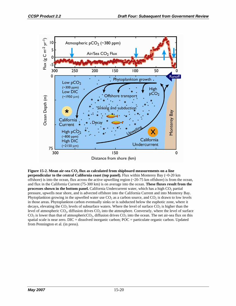
CCSP Product 2.2 Draft Four: Subsequent from Government Review
May 2007 15-20
Figure 15-2. Mean air-sea CO2 flux as calculated from shipboard measurements on a line perpendicular to the central California coast (top panel). Flux within Monterey Bay (~0-20 km offshore) is into the ocean, flux across the active upwelling region (~20-75 km offshore) is from the ocean, and flux in the California Current (75-300 km) is on average into the ocean. These fluxes result from the processes shown in the bottom panel. California Undercurrent water, which has a high CO2 partial pressure, upwells near shore, and is advected offshore into the California Current and into Monterey Bay. Phytoplankton growing in the upwelled water use CO2 as a carbon source, and CO2 is drawn to low levels in those areas. Phytoplankton carbon eventually sinks or is subducted below the euphotic zone, where it decays, elevating the CO2 levels of subsurface waters. Where the level of surface CO2 is higher than the level of atmospheric CO2, diffusion drives CO2 into the atmosphere. Conversely, where the level of surface CO2 is lower than that of atmosphericCO2, diffusion drives CO2 into the ocean. The net air-sea flux on this spatial scale is near zero. DIC = dissolved inorganic carbon; POC = particulate organic carbon. Updated from Pennington et al. (in press).

CCSP Product 2.2 Draft Four: Subsequent from Government Review
May 2007 15-21
(A)
(B)
Figure 15-3. (A). Distribution of coastal surface water CO2 partial pressure measurements made between 1979 and 2004. (B). The distribution of the annual mean air-sea net CO2 flux over 1° × 1° pixel areas (N-S 100 km, E-W 80 km) around North America. The flux (grams of carbon per square meter per year) represents the climatological mean over the 25-year period. The magenta-blue colors indicate that the ocean water is a sink for atmospheric CO2, and the green-yellow-orange colors indicate that the sea is a CO2 source. The data were obtained by the authors and collaborators of this chapter and are archived at the Lamont-Doherty Earth Observatory (www.ldeo.columbia.edu/res/pi/CO2).
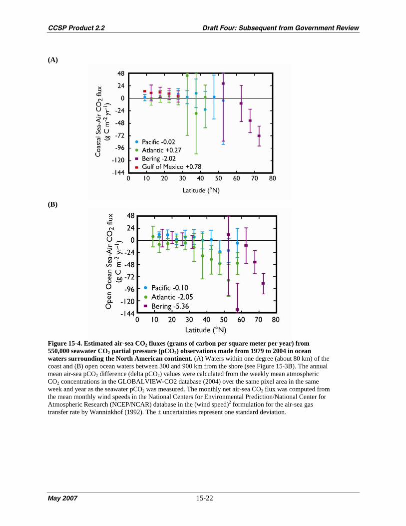
CCSP Product 2.2 Draft Four: Subsequent from Government Review
May 2007 15-22
(A)
(B)
Figure 15-4. Estimated air-sea CO2 fluxes (grams of carbon per square meter per year) from 550,000 seawater CO2 partial pressure (pCO2) observations made from 1979 to 2004 in ocean waters surrounding the North American continent. (A) Waters within one degree (about 80 km) of the coast and (B) open ocean waters between 300 and 900 km from the shore (see Figure 15-3B). The annual mean air-sea pCO2 difference (delta pCO2) values were calculated from the weekly mean atmospheric CO2 concentrations in the GLOBALVIEW-CO2 database (2004) over the same pixel area in the same week and year as the seawater pCO2 was measured. The monthly net air-sea CO2 flux was computed from the mean monthly wind speeds in the National Centers for Environmental Prediction/National Center for Atmospheric Research (NCEP/NCAR) database in the (wind speed)2 formulation for the air-sea gas transfer rate by Wanninkhof (1992). The ± uncertainties represent one standard deviation.

CCSP Product 2.2 Draft Four: Subsequent from Government Review
May 2007 15-23
(A)
(B)
Figure 15-5. Time-space variability of coastal waters off the west coast of North America. (A) Quasi-synoptic distribution of the temperature, salinity, and pCO2 in surface waters during July-September 2005. The Columbia River plume (~46°N) and the upwelling of deep waters off the Cape Mendocino (~40°N) are clearly seen. (B) 1997-2005 time-series data for air-sea CO2 flux from a mooring off Monterey Bay, California. Seawater is a CO2 source for the atmosphere during the summer upwelling events, but biological uptake reduces levels very rapidly. These rapid fluctuations can affect atmospheric CO2 levels. For example, if CO2 from the sea is mixed into a static column, a 500-m-thick planetary boundary layer over the course of one day, atmospheric CO2 concentration would change by 2.5 µatm. If the column of air is mixed vertically through the troposphere to 500 mbar, a change of about 0.5 µatm would occur. The effects would be diluted as the column of air mixes laterally. However, this demonstrates that the large fluctuations of air-sea CO2 flux observed over coastal waters could affect the concentration of CO2 significantly enough to affect estimates of air-land flux based on the inversion of

CCSP Product 2.2 Draft Four: Subsequent from Government Review
May 2007 15-24
atmospheric CO2 data. Air-sea CO2 flux was low during the 1997-1998 and 2002-2003 El Niño periods. The shaded areas indicate the 1997-98 and 2002-2003 El Niño episodes. The greatest El Niño anomalies occur in the winter which is the period of lowest air-sea fluxes.
CCSP Product 2.2 Draft Four: Subsequent from Government Review
May 2007 A-1
GLOSSARY afforestation The establishment of trees on land that has lacked forest cover for a very long
period of time or has never been forested
anthropogenic Human-induced; produced by or resulting from human activity
apparent consumption The amount or quantity expressed by the following formula: production + imports – exports +/– changes in stocks
biomass The mass of living organic matter (plant and animal) in an ecosystem. Biomass also refers to organic matter (living and dead) available on a renewable basis for use as a fuel. Biomass includes trees and plants (both terrestrial and aquatic), agricultural crops and wastes, wood and wood wastes, forest and mill residues, animal wastes, livestock operation residues, and some municipal and industrial wastes
carbon sequestration The process of increasing the carbon content of a carbon reservoir other than the atmosphere. Often used narrowly to refer to increasing the carbon content of carbon pools in the biosphere and distinguished from physical or chemical collection of carbon followed by injection into geologic reservoirs, which is generally referred to as “carbon capture and storage.”
carbon cycle The term used to describe the flow of carbon [in various forms such as carbon dioxide (CO2), organic matter, and carbonates] through the atmosphere, ocean, terrestrial biosphere, and lithosphere
carbon equivalent The amount of carbon in the form of carbon dioxide that would produce the same effect on the radiative balance of the Earth’s climate system. Applicable in this report to greenhouse gases such as methane (CH4).
carbon intensity The relative amount of carbon emitted per unit of energy or fuels consumed
coastal waters The region within 100 km from shore in which coastal processes influence the partial pressure of CO2 in surface sea waters
CO2 equivalent The amount of carbon dioxide that would produce the same effect on the radiative balance of the Earth’s climate system as another greenhouse gas, such as methane (CH4).

CCSP Product 2.2 Draft Four: Subsequent from Government Review
May 2007 A-2
CO2 fertilization The phenomenon in which plant growth increases (and agricultural crop yields increase) due to the increased rates of photosynthesis of plant species in response to elevated concentrations of CO2 in the atmosphere
decarbonization Reduction in the use of carbon-based energy sources as a proportion of total energy supplies or increased use of carbon-based fuels with lower values of carbon content per unit of energy content.
dry climates Climates where the ratio of mean annual precipitation to potential evapotranspiration is less than 1.0
ecosystem A community (i.e., an assemblage of populations of plants, animals, fungi, and microorganisms that live in an environment and interact with one another, forming together a distinctive living system with its own composition, structure, environmental relations, development, and function) and its environment treated together as a functional system of complementary relationships and transfer and circulation of energy and matter.
energy intensity The relative amount or ratio of the consumption of energy to the resulting amount of output, service or activity (i.e., expressed as energy per unit of output)
feebates Systems of progressive vehicle taxes on purchases of less efficient new vehicles and subsidies for more efficient new vehicles
fossil fuels Fuels such as coal, petroleum, and natural gas derived from the chemical and physical transformation (fossilization) of the remains of plants and animals that lived during the Carboniferous Period 360–286 million years ago
global warming potential (GWP)
A factor describing the radiative forcing impact (e.g., warming of the atmosphere) of one unit mass of a given greenhouse gas relative to the warming caused by a similar mass of carbon dioxide. Methane (CH4), for example, has a GWP of 23.
greenhouse gases (GHGs)
Greenhouse gases are those gaseous constituents of the atmosphere, both natural and anthropogenic, that absorb and emit radiation at specific wavelengths within the spectrum of infrared radiation emitted by the Earth’s surface, the atmosphere, and clouds. This property causes the greenhouse effect. Water vapor (H2O), carbon dioxide (CO2), nitrous oxide (N2O), methane (CH4), and ozone (O3) are the primary greenhouse gases in the Earth’s atmosphere. Moreover there are a number of entirely human-made greenhouse gases in the atmosphere, such as the halocarbons and other chlorine and bromine-containing substances, dealt with under the Montreal Protocol.

CCSP Product 2.2 Draft Four: Subsequent from Government Review
May 2007 A-3
leakage
The part of emissions reductions in Annex B countries that may be offset by an increase of the emission in the non-constrained countries above their baseline levels. This can occur through (1) relocation of energy-intensive production in non-constrained regions; (2) increased consumption of fossil fuels in these regions through decline in the international price of oil and gas triggered by lower demand for these energies; and (3) changes in incomes (and thus in energy demand) because of better terms of trade. “Leakage” also refers to the situation in which a carbon sequestration activity (e.g., tree planting) on one piece of land inadvertently, directly or indirectly, triggers an activity, which in whole or part, counteracts the carbon effects of the initial activity.
mitigation A human intervention to reduce the sources of or to enhance the sinks of greenhouse gases
net ecosystem exchange (NEE)
The net flux of carbon between the land and the atmosphere, typically measured using eddy covariance techniques. Note: NEE and NEP are equivalent terms but are not always identical because of measurement and scaling issues.
net ecosystem production (NEP)
The net carbon accumulation within the ecosystem after all gains and losses are accounted for, typically measured using ground-based techniques
net primary production (NPP)
The net uptake of carbon by plants in excess of respiratory loss
North America The combined land area of Canada, the United States of America, and Mexico and their coastal waters
North American Carbon Program (NACP)
A multidisciplinary research program, supported by a number of different U.S. federal agencies through a variety of intramural and extramural funding mechanisms and award instruments, to obtain scientific understanding of North America’s carbon sources and sinks and of changes in carbon stocks needed to meet societal concerns and to provide tools for decision makers.
ocean acidification The phenomenon in which the pH of the oceans becomes more acidic due to increased levels of CO2 in the atmosphere which, in turn, increase the amount of dissolved CO2 in sea water
option A choice among a set of possible measures or alternatives
peatlands Areas characterized as having an organic layer thickness of at least 30 cm (note, the current U.S. and Canadian soil taxonomies specify a minimum thickness of 40 cm)

CCSP Product 2.2 Draft Four: Subsequent from Government Review
May 2007 A-4
permafrost Soils or rocks that remain below 0° C for at least two consecutive years
pool/reservoir Any natural region or zone, or any artificial holding area, containing an accumulation of carbon or carbon-bearing compounds or having the potential to accumulate such substances
sink In general, any process, activity or mechanism which removes a greenhouse gas or a precursor of a greenhouse gas or aerosol from the atmosphere. In this report, a sink is any regime or pool in which the amount of carbon is increasing (i.e., is being accumulated or stored).
source In general, any process, activity or mechanism which releases a greenhouse gas or a precursor of a greenhouse gas or aerosol into the atmosphere. In this report, a source is any regime or pool in which the amount of carbon is decreasing (i.e., is being released or emitted).
stocks The amount or quantity contained in the inventory of a pool or reservoir
temperate zones Regions of the earth’s surface located above 30º latitude and below 66.5º latitude
trend A systematic change over time
tropical zones Regions located between the earth’s equator and 30º latitude (this area includes subtropical regions)
uncertainty An expression of the degree to which a value is unknown. Uncertainty can result from lack of information or from disagreement about what is known or even knowable. It may have many types of sources, from quantifiable errors in the data to ambiguously defined concepts or terminology, or uncertain projections of human behavior. Uncertainty can therefore be represented by quantitative measures (e.g., a range of values calculated by various models) or by qualitative statements (e.g., reflecting the judgment of a team of experts), or can sometimes be expressed in terms of probability or likelihood
wet climates Climates where the ratio of mean annual precipitation to potential evapotranspiration is greater than 1.0
wetlands Areas that are inundated or saturated by surface water or groundwater at a frequency and duration sufficient to support—and that under normal circumstances do support—a prevalence of vegetation typically adapted for life in saturated soil conditions, including swamps, marshes, bogs, and similar areas

CCSP Product 2.2 Draft Four: Subsequent from Government Review
May 2007 B-1
ACRONYMS AND ABBREVIATIONS
µatm microatmosphere (a measure of pressure)
ACEEE American Council for an Energy-Efficient Economy
CAFE Corporate Average Fuel Economy
CAIT Climate Analysis Indicators Tool
CAST Council for Agricultural Science and Technology
CBO U.S. Congressional Budget Office
CCSP U.S. Climate Change Science Program
CCTP Climate Change Technology Program
CDIAC Carbon Dioxide Information Analysis Center
CEC California Energy Commission
CH4 methane
CIEEDAC Canadian Industrial Energy End-Use Data and Analysis Centre
CO carbon monoxide
CO2 carbon dioxide
CO3 carbonate
COP Conference of Parties
DOC dissolved organic carbon
DOE U.S. Department of Energy
DOT U.S. Department of Transportation
EIA Energy Information Administration
EPA U.S. Environmental Protection Agency
ESCOs energy services companies
FAO Food and Agriculture Organization
FWMS freshwater mineral-soil
g gram
GAO U.S. Government Accountability Office
GDP gross domestic product
GHG greenhouse gas
Gt C gigatons of carbon (billions of metric tons; i.e., petagrams)
GWP global warming potential
ha hectare
CCSP Product 2.2 Draft Four: Subsequent from Government Review
May 2007 B-2
HCO3 bicarbonate
ICLEI International Council for Local Environmental Initiatives (now known as
International Governments for Local Sustainability)
IOOS Integrated Ocean Observing System
IPCC Intergovernmental Panel on Climate Change
IWG Interlaboratory Working Group
kg kilogram
km kilometer
L liter
LEED Leadership in Energy and Environment Design
m meter
MAP mean annual precipitation
mpg miles per gallon
Mt C megatons of carbon (millions of metric tons; i.e., teragrams)
N2O nitrous oxide (also, dinitrogen oxide)
NACP North American Carbon Program
NAO North Atlantic oscillation
NAS U.S. National Academy of Sciences
NASA National Aeronautics and Space Administration
NATS North American Transportation Statistics
NCAR National Center for Atmospheric Research
NCEP National Centers for Environmental Prediction; National Commission on Energy
Policy
NEE net ecosystem exchange
NEP net ecosystem productivity
NGO non-governmental organization
NO2 nitric oxide (also, nitrogen dioxide)
NOAA National Oceanic and Atmospheric Administration
NOx oxides of nitrogen
NPP net primary productivity
NRC National Research Council
NRCS National Resources Conservation Service
NSF National Science Foundation
CCSP Product 2.2 Draft Four: Subsequent from Government Review
May 2007 B-3
NWI National Wetland Inventory
OCCC Ocean Carbon and Climate Change
pCO2 partial pressure of carbon dioxide
PDO Pacific decadal oscillation
PET potential evapotranspiration
PJ petajoules
ppm parts per million
PPP purchasing power parity
RGGI Regional Greenhouse Gas Initiative
SAP Synthesis and Assessment Product
SBSTA Subsidiary Body for Scientific and Technological Advice
SOCCR State of the Carbon Cycle Report
UNFCCC United Nations Framework Convention on Climate Change
USDA U.S. Department of Agriculture
VOCs volatile organic compounds
WBCSD World Business Council for Sustainable Development
yr year

CCSP Product 2.2 Draft Four: Subsequent from Government Review
May 2007 B-4
[This page intentionally left blank]

CCSP Product 2.2 Draft Four: Subsequent from Government Review
May 2007 3A-1
APPENDIX 3A
Historical Overview of the Development of United States, Canadian, and Mexican Ecosystem Sources and Sinks for Atmospheric Carbon
Although the lands of the New World were inhabited before the arrival of Europeans, the changes
since arrival have been enormous, especially during the last two centuries. Peak United States emissions
from land-use change occurred late in the nineteenth century, and the last few decades have experienced a
carbon sink (Houghton et al., 1999; Hurtt et al., 2002). In Canada, peak emissions occurred nearly a
century later than in the United States, and current data show that land-use change causes a net carbon
sink (Environment Canada, 2005). In Mexico, the emissions of carbon continue to increase from net
deforestation. All three countries may be in different stages of the same development pattern (see Fig. 3-
2).
The largest changes in land use and the largest emissions of carbon came from the expansion of
croplands. In addition to the carbon lost from trees, soils lose 25-30% of their initial carbon content (to a
depth of 1 m) when cultivated. In the United States, croplands increased from about 0.25 million hectare
in 1700 to 236 million hectare in 1990 (Houghton et al., 1999; Houghton and Hackler, 2000). The most
rapid expansion (and the largest emissions) occurred between 1800 and 1900, and since 1920 there has
been little net change in cropland area. Pastures expanded nearly as much, from 0.01 million to 231
million hectare, most of the increase taking place between 1850 and 1950. As most pastures were derived
from grasslands, the associated changes in carbon stocks were modest.
The total area of forests and woodlands in the United States declined as a result of agricultural
expansion by 160 million hectare (38%), but this net change obscures the dynamics of forest loss and
recovery, especially in the eastern part of the United States. After 1920, forest areas increased by 14
million hectare nationwide as farmlands continued to be abandoned in the northeast, southeast, and north
central regions. Nevertheless, another 4 million hectare of forest were lost in other regions, and the net
recovery of 10 million hectare offset only 6% of the net loss (Houghton and Hackler, 2000).
Between 1938 and 2002, the total area of forest land in the conterminous United States decreased
slightly, by 3 million hectare (Smith et al., 2004). This small change is the net result of much larger shifts
among land-use classes (Birdsey and Lewis, 2003). Gains of forest land, primarily from cropland and
pasture, were about 50 million hectare for this period. Losses of forest land to cropland, pasture, and
developed use were about 53 million hectare for the same period. Gains of forest land were primarily in

CCSP Product 2.2 Draft Four: Subsequent from Government Review
May 2007 3A-2
the Eastern United States, whereas losses to cropland and pasture were predominantly in the South, and
losses to developed use were spread around all regions of the United States.
In the United States, harvest of industrial wood (timber) generally followed the periods of major
agricultural clearing in each region. In the last few decades, total volume harvested increased until a
recent leveling took place (Smith et al., 2004). The volume harvested in the Pacific Coast and Rocky
Mountain regions has declined sharply, whereas harvest in the South increased and in the North, stayed
level. Fuel wood harvest peaked between 1860 and 1880, after which fossil fuels became the dominant
type of fuel (Houghton and Hackler, 2000).
The arrival of Europeans reduced the area annually burned, but a federal program of fire protection
was not established until early in the twentieth century. Fire exclusion had begun earlier in California and
in parts of the central, mountain and Pacific regions. However, neither the extent nor the timing of early
fire exclusion is well known. After about 1920, the Cooperative Fire Protection Program gradually
reduced the areas annually burned by wildfires (Houghton et al., 1999, 2000). The reduction in wildfires
led to an increase in carbon storage in forests. How long this “recovery” will last is unclear. There is some
evidence that fires are becoming more widespread, again, especially in Canada and the western United
States. Fire exclusion and suppression are also thought to have led to woody encroachment, especially in
the southwestern and western United States. The extent and rate of this process is poorly documented,
however, and estimates of a carbon sink are very uncertain. Gains in carbon above ground may be offset
by losses belowground in some systems, and the spread of exotic annual grasses into semiarid deserts and
shrublands may be converting the recent sink to a source (Bradley et al., in preparation).
The consequence of this land-use history is that United States forests, at present, are recovering from
agricultural abandonment, fire suppression, and reduced logging (in some regions), and, as a result, are
accumulating carbon (Birdsey and Heath, 1995; Houghton et al., 1999; Caspersen et al., 2000; Pacala et
al., 2001). The magnitude of the sink is uncertain, and whether any of it has been enhanced by
environmental change (CO2 fertilization, nitrogen deposition, and changes in climate) is unclear.
Understanding the mechanisms responsible for the current sink is important for predicting its future
behavior (Hurtt et al., 2002).
In the mid-1980s, Mexico lost approximately 668,000 hectare of closed forests annually, about 75%
of them tropical forests (Masera et al., 1997). Most deforestation was for pastures. Another 136,000
hectare of forest suffered major perturbations, and the net flux of carbon from deforestation, logging,
fires, degradation, and the establishment of plantations was 52.3 million tons of carbon per year, about
40% of the country’s estimated annual emissions of carbon. A later study found the deforestation rate for
tropical Mexico to be about 12% higher (1.9% per year) (Cairns et al., 2000).

CCSP Product 2.2 Draft Four: Subsequent from Government Review
May 2007 3A-3
REFERENCES FOR APPENDIX 3A
Birdsey, R.A. and L.S. Heath, 1995: Carbon changes in U.S. forests. In: Productivity of America’s Forests and
Climate Change [Joyce, L.A. (ed.)]. General Technical Report RM-GTR-271, U.S. Department of Agriculture,
Forest Service, Rocky Mountain Forest and Range Experiment Station, Fort Collins, CO, pp. 56-70.
Birdsey, R.A. and G.M. Lewis, 2003: Current and historical trends in use, management, and disturbance of U.S.
forestlands. In: The Potential of U.S. Forest Soils to Sequester Carbon and Mitigate the Greenhouse Effect
[Kimble, J.M., L.S. Heath, and R. A. Birdsey (eds.)]. CRC Press LLC, New York, NY, pp. 15-33.
Bradley, B.A., R.A. Houghton, J.F. Mustard, and S.P. Hamburg, 2006: Invasive grass reduces carbon stocks in
shrublands of the Western U.S. (in press).
Cairns, M.A., P.K. Haggerty, R. Alvarez, B.H.J. De Jong, and I. Olmsted, 2000: Tropical Mexico’s recent land-use
change: a region’s contribution to the global carbon cycle. Ecological Applications, 10(5), 1426-1441.
Caspersen, J.P., S.W. Pacala, J.C. Jenkins, G.C. Hurtt, P.R. Moorcroft, and R.A. Birdsey, 2000: Contributions of
land-use history to carbon accumulation in U.S. forests. Science, 290, 1148-1151.
Environment Canada, 2005: Canada’s Greenhouse Gas Inventory 1990-2003: Initial Submission. Greenhouse Gas
Division, Environment Canada, Ottawa, Ontario, Canada. Available at http://unfccc.int/national_reports/
annex_i_ghg_inventories/national_inventories_submissions/items/2761.php
Houghton, R.A., J.L. Hackler, and K.T. Lawrence, 1999: The U.S. carbon budget: contributions from land-use
change. Science, 285, 574-578.
Houghton, R.A. and J.L. Hackler, 2000: Changes in terrestrial carbon storage in the United States. 1. The roles of
agriculture and forestry. Global Ecology and Biogeography, 9, 125-144.
Houghton, R.A., J.L. Hackler, and K.T. Lawrence, 2000: Changes in terrestrial carbon storage in the United States.
2. The role of fire and fire management. Global Ecology and Biogeography, 9, 145-170.
Hurtt, G.C., S.W. Pacala, P.R. Moorcroft, J. Caspersen, E. Shevliakova, R.A. Houghton, and B. Moore III, 2002:
Projecting the future of the U.S. carbon sink. Proceedings of the National Academy of Sciences of the United
States of America, 99, 1389-1394.
Masera, O.R., M.J. Ordonez, and R. Dirzo, 1997: Carbon emissions from Mexican forests: current situation and
long-term scenarios. Climate Change, 35, 265-295.
Pacala, S.W., G.C. Hurtt, R.A. Houghton, R.A. Birdsey, L. Heath, E.T. Sundquist, R.F. Stallard, D. Baker,
P. Peylin, P. Moorcroft, J. Caspersen, E. Shevliakova, M.E. Harmon, S.-M. Fan, J.L. Sarmiento, C. Goodale,
C.B. Field, M. Gloor, and D. Schimel, 2001: Consistent land- and atmosphere-based U.S. carbon sink estimates.
Science, 292(5525), 2316-2320.
Smith, W.B., P.D. Miles, J.S. Vissage, and S.A. Pugh, 2004: Forest Resources of the United States, 2002. General
Technical Report NC-241, U.S. Department of Agriculture, Forest Service, St. Paul, MN, 137 pp.

CCSP Product 2.2 Draft Four: Subsequent from Government Review
May 2007 3A-4
[This page intentionally left blank] 1

CCSP Product 2.2 Draft Four: Subsequent from Government Review
May 2007 3B-1
APPENDIX 3B
Eddy-Covariance Measurements Now Confirm Estimates of Carbon Sinks from Forest Inventories
Long-term, tower-based, eddy-covariance measurements (e.g., Wofsy et al., 1993) represent an
independent approach to measuring ecosystem-atmosphere CO2 exchange. The method describes fluxes
over areas of approximately 1 km2 (Horst and Weil, 1994), measures hour-by-hour ecosystem carbon
fluxes, and can be integrated over time scales of years. A network of more than 200 sites now exists
globally (Baldocchi et al., 2001); more than 50 of these are in North America. None of these sites existed
in 1990, so these represent a relatively new source of information about the terrestrial carbon cycle. An
increasing number of these measurement sites include concurrent carbon inventory measurements.
Where eddy-covariance and inventory measurements are concurrent, the rates of accumulation or loss
of biomass are often consistent to within several tens of g C m-2 per year for a one-year sample (10 g C
per year is 5% of a typical net sink of 2 metric tons of carbon per hectare per year for an Eastern
deciduous successional forest). Published intercomparisons in North America exist for western coniferous
forests (Law et al., 2001), agricultural sites (Verma et al., 2005), and eastern deciduous forests (Barford et
al., 2001; Cook et al., 2004; Curtis et al., 2002; Ehmann et al., 2002; Gough et al., in review). Multiyear
studies at two sites (Barford et al., 2001; Gough et al., in review) show that 5- to 10-year averages
converge toward inventory measurements. Table 3B-1 from Barford et al. (2001) shows the results of
nearly a decade of concurrent measurements in an eastern deciduous forest.
This concurrence between eddy-covariance flux measurements and ecosystem carbon inventories is
relevant because it provides independent validation of the inventory measurements used to estimate long-
term trends in carbon stocks. The eddy-covariance data are also valuable because the assembly of global
eddy-covariance data provides independent support for net storage of carbon by many terrestrial
ecosystems and the substantial year-to-year variability in this net sink. The existence of the eddy-
covariance data also makes the sites suitable for co-locating mechanistic studies of interannual and
shorter, time-scale processes governing the terrestrial carbon cycle. Chronosequences show trends
consistent with inventory assessments of forest growth, and comparisons across space and plant
functional types are beginning to show broad consistency. These results show a consistency across a
mixture of observational methods with complementary characteristics, which should facilitate the
development of an increasingly complete understanding of continental carbon dynamics (Canadell et al.,
2000).

CCSP Product 2.2 Draft Four: Subsequent from Government Review
May 2007 3B-2
REFERENCES FOR APPENDIX 3B
Baldocchi, D., E. Falge, L.H. Gu, R. Olson, D. Hollinger, S. Running, P. Anthoni, C. Bernhofer, K. Davis,
R. Evans, J. Fuentes, A. Goldstein, G. Katul, B. Law, X.H. Lee, Y. Malhi, T. Meyers, W. Munger, W. Oechel,
K.T. Paw U, K. Pilegaard, H.P. Schmid, R. Valentini, S. Verma, T. Vesala, K. Wilson, and S. Wofsy, 2001:
FLUXNET: a new tool to study the temporal and spatial variability of ecosystem-scale carbon dioxide, water
vapor, and energy flux densities, Bulletin of the American Meteorological Society, 82, 2415-2434.
Barford, C.C., S.C. Wofsy, M.L. Goulden, J.W. Munger, E.H. Pyle, S.P. Urbanski, L. Hutyra, S.R. Saleska,
D. Fitzjarrald, and K. Moore, 2001: Factors controlling long- and short-term sequestration of atmospheric CO2
in a mid-latitude forest. Science, 294, 1688-1691.
Canadell, J.G., H.A. Mooney, D.D. Baldocchi, J.A. Berry, J.R. Ehleringer, C.B. Field, S.T. Gower, D.Y. Hollinger,
J.E. Hunt, R.B. Jackson, S.W. Running, G.R. Shaver, W. Steffen, S.E. Trumbore, R. Valentini, B.Y. Bond,
2000: Carbon metabolism of the terrestrial biosphere: a multitechnique approach for improved understanding.
Ecosystems, 3, 115-130.
Cook, B.D., K.J. Davis, W. Wang, A. Desai, B.W. Berger, R.M. Teclaw, J.G. Martin, P.V. Bolstad, P.S. Bakwin, C.
Yi, and W. Heilman, 2004: Carbon exchange and venting anomalies in an upland deciduous forest in northern
Wisconsin, USA. Agricultural and Forest Meteorology, 126, 271-295.
Curtis, P.S., P.J. Hanson, P. Bolstad, C. Barford, J.C. Randolph, H.P. Schmid, and K.B. Wilson, 2002: Biometric
and eddy-covariance based estimates of annual carbon storage in five eastern North American deciduous
forests. Agricultural and Forest Meteorology, 113, 3-19.
Ehman, J.L., H.P. Schmid, C.S.B. Grimmond, J.C. Randolph, P.J. Hanson, C.A. Wayson, and F.D. Cropley, 2002:
An initial intercomparison of micrometerological and ecological inventory estimates of carbon exchange in a
mid-latitude deciduous forest. Global Change Biology, 8, 575-589.
Gough, C.M., P.S. Curtis, J.G. Vogel, H.P. Schmid, and H.B. Su: Annual carbon storage from 1999 to 2003 in a
Northern hardwood forest assessed using eddy-covariance and biometric methods. Agricultural and Forest
Meteorology (in review).
Horst, T.W. and J.C. Weil, 1994: How far is far enough? The fetch requirements for micrometeorological
measurement of surface fluxes. Journal of Atmospheric and Oceanic Technology, 11, 1018-1025.
Law, B.E., P.E. Thornton, J. Irvine, P.M. Anthoni, and S. Van Tuyl, 2001: Carbon storage and fluxes in ponderosa
pine forests at different developmental stages. Global Change Biology, 7, 755-777.
Verma, S.B., A. Dobermann, K.G. Cassman, D.T. Walters, J.M. Knops, T.J. Arkebauer, A.E. Suyker, G.G. Burba,
B. Amos, H.S. Yang, D. Ginting, K.G. Hubbard, A.A. Gitelson, and E.A. Walter-Shea, 2005: Annual carbon
dioxide exchange in irrigated and rainfed maize-based agroecosystems. Agricultural and Forest Meteorology,
131, 77-96.
Wofsy, S.C., M.L. Goulden, J.W. Munger, S.-M. Fan, P.S. Bakwin, B.C. Daube, S.L. Bassow, and F.A. Bazzaz.
1993: Net exchange of CO2 in a mid-latitude forest. Science, 260, 1314-1317.
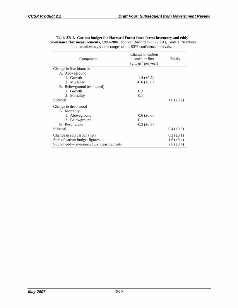
CCSP Product 2.2 Draft Four: Subsequent from Government Review
May 2007 3B-3
Table 3B-1. Carbon budget for Harvard Forest from forest inventory and eddy-
covariance flux measurements, 1993-2001. Source: Barford et al. (2001), Table 1. Numbers in parentheses give the ranges of the 95% confidence intervals.
Component Change in carbon
stock or flux (g C m-2 per year)
Totals
Change in live biomass A. Aboveground
1. Growth 2. Mortality
B. Belowground (estimated) 1. Growth 2. Mortality
Subtotal
1.4 (±0.2) -0.6 (±0.6)
0.3
-0.1
1.0 (±0.2)
Change in dead wood A. Mortality
1. Aboveground 2. Belowground
B. Respiration Subtotal
0.6 (±0.6) 0.1
-0.3 (±0.3)
0.4 (±0.3)
Change in soil carbon (net) 0.2 (±0.1) Sum of carbon budget figures 1.6 (±0.4) Sum of eddy-covariance flux measurements 2.0 (±0.4)

CCSP Product 2.2 Draft Four: Subsequent from Government Review
May 2007 3B-4
[This page intentionally left blank] 1
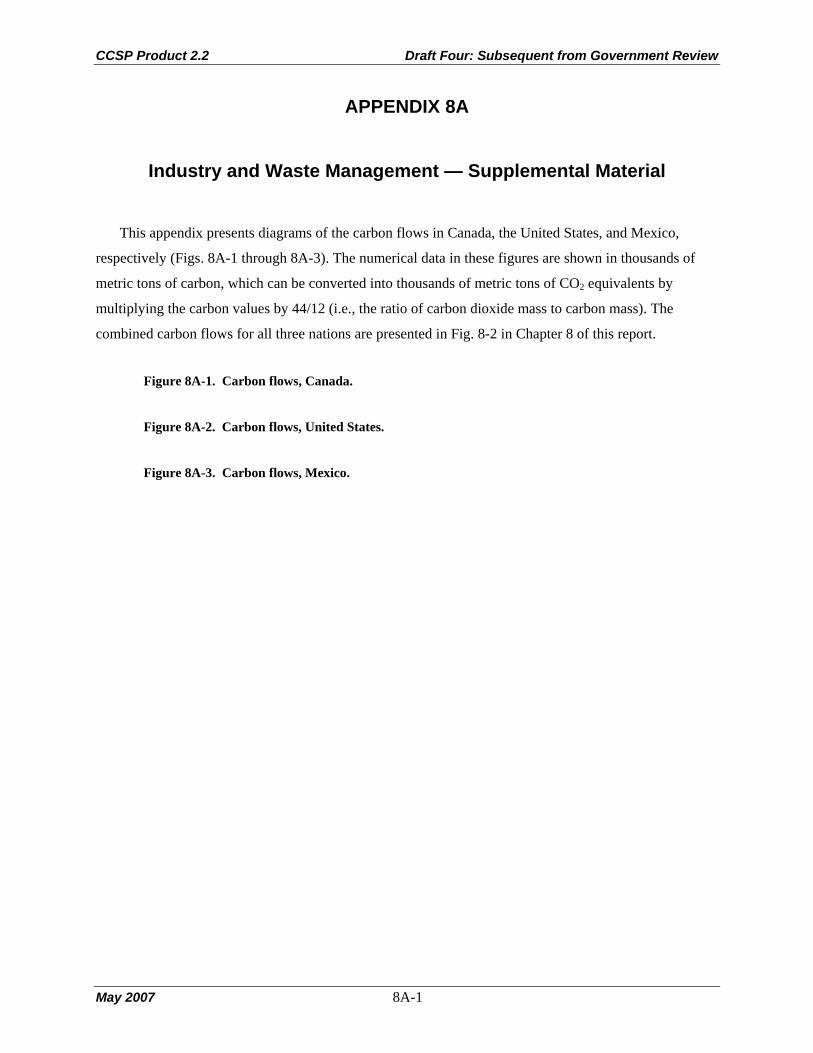
CCSP Product 2.2 Draft Four: Subsequent from Government Review
May 2007 8A-1
APPENDIX 8A
Industry and Waste Management — Supplemental Material
This appendix presents diagrams of the carbon flows in Canada, the United States, and Mexico,
respectively (Figs. 8A-1 through 8A-3). The numerical data in these figures are shown in thousands of
metric tons of carbon, which can be converted into thousands of metric tons of CO2 equivalents by
multiplying the carbon values by 44/12 (i.e., the ratio of carbon dioxide mass to carbon mass). The
combined carbon flows for all three nations are presented in Fig. 8-2 in Chapter 8 of this report.
Figure 8A-1. Carbon flows, Canada.
Figure 8A-2. Carbon flows, United States.
Figure 8A-3. Carbon flows, Mexico.

CCSP Product 2.2 Draft Four: Subsequent from Government Review
May 2007 8A-2
Wood Products
Food Products
Iron and Steel
Cement
Chemical Plants
Energy 3,079
Logs 36,185
C fixed from Photosynthesis 7,042Coking Coal 3,067
Lime 1,862
Materials and Energy 11,761
Wood Products 11,908
Food Products 7,114
Iron and Steel Products 80
Chemical Products 4,898
Emissions from Fuel Combustion 24,314
Process Emissions 5,457
Other Products and Waste14,818
Canada Carbon Flows (All Values in Kilotonnes of C)
Energy 1,744
Energy 1,245
Energy 2,226
Pulp and Paper 12,574
Total Flow: 81,163
Other IndustriesEnergy 12,953
Process Emissions include Emissions from Iron and Steel, Agriculture, Cement & Lime, and Chemical Industries
Fig. 8A-1. Carbon flows, Canada. Source: Energy data from Statistics Canada Industrial Consumption of Energy survey, conversion coefficients and process emissions from Environment Canada, Canada GHG Inventory, 2002. Production data from Statistics Canada, CANSIM Table 002-0010, Tables 303-0010, -0014 to -0021, -0024, -0060, Pub. Cat. Nos.: 21-020, 26-002, 45-002, Canadian Pulp and Paper Association on forestry products.

CCSP Product 2.2 Draft Four: Subsequent from Government Review
May 2007 8A-3
Wood Products
Food Products
Iron and Steel
Cement
Chemical Plants
Energy 18,766
Logs 91,054
C fixed from Photosynthesis 238,664Coking Coal 19,182
Lime 15,028
Materials and Energy 112,818
Wood and Paper Products 82,206
Food Products 234,455
US Carbon Flows (All Values in Kilotonnes of C)
Iron and Steel Products 461
Chemical Products 3,094
Process Emissions 42,322
Other Products and Waste 95,026
Energy 2,011
Energy 9,332
Energy 13,843
Emissions from fuel combustion 169,484
Total Flow: 627,048
Other IndustriesMaterials and Energy 106,350
Process Emissions include Emissions from Iron and Steel, Agriculture, Cement & Lime, and Chemical Industries
Fig. 8A-2. Carbon flows, United States. Source: Energy data from IEA Oil Information 2004, IEA Coal Information 2005, IEA Natural Gas Information 2004. Process emissions: EPA, U.S. Emissions Inventory. Production of forestry products: USDA Database; FO-2471000 and -2472010, U.S. Timber Production, Trade, Consumption, and Price Statistics 1965-2005, Production of organic products (e.g., food): USDA PS&D Official Statistical Results, Steel: International Iron and Steel institute, World steel in figures 2003, Minerals production: USGS mineral publications.

CCSP Product 2.2 Draft Four: Subsequent from Government Review
May 2007 8A-4
Wood Products
Food Products
Iron and Steel
Chemical Plants
Energy 362
Energy 1,690Energy 1,840
Materials and Energy 6,718
Wood and Paper Products 491
Food Products 25,561
Mexico Carbon Flows (All Values in Kilotonnes of C)
Iron and Steel Products 71
Emission from Fuel Combustion 13,118
Other Products and Waste 3,761
*Insufficient Data for the inclusion of the Cement Industry, data estimated from CAIT data
Coking Coal 1,630
C fixed from Photosynthesis 25,545
Logs 1,078
Total Flow: 50,686
Chemical Products 3,459
Other Industries
Energy 7,596 Process Emissions 4,227
CementMaterials and Energy 4,227
Fig. 8A-3. Carbon flows, Mexico. Source: Energy data from IEA Oil Information 2004, IEA Coal Information 2005, IEA Natural Gas Information 2004. Process emissions: EPA, U.S. Emissions Inventory. Production of forestry products: USDA Database; FO-2471000, -2472010, -2482000, -2483040, -6342000, -6342040. Production of organic products (e.g., food): USDA PS&D Official Statistical Results. Steel: International Iron and Steel institute, World steel in figures 2003.

CCSP Product 2.2 Draft Four: Subsequent from Government Review
May 2007 11A-1
APPENDIX 11A
Ecosystem Carbon Fluxes
The recent history of disturbance largely determines whether a forest system will be a net source or
sink of carbon (C). For example, net ecosystem productivity (NEP, gains due to biomass growth minus
losses due to respiration in vegetation and soil) is being measured across a range of forest types in Canada
using the eddy covariance technique. See Table 11A-1 for a list of definitions and acronyms used in this
appendix.
In mature forests, values range from -19.6 t C ha-1 per year in a white pine plantation in southern
Ontario (Arain and Restrepo-Coupe, 2005) to -3.2 t C ha-1 per year in a jack pine forest in (Amiro et al.,
2005; Griffis et al., 2003). In recently disturbed forests, NEP ranges from +58.0 t C ha-1 per year in a
harvested Douglas-fir forest (Humphreys et al., 2005) to +5.7 t C ha-1 per year in a 7 year old harvested
jack pine forest (Amiro et al., 2005). In general, forest stands recovering from disturbance are sources of
carbon until uptake from growth becomes greater than losses due to respiration, usually within 10 years
(Amiro et al., 2005).
In the United States, extensive land-based measurements of forest/atmosphere carbon exchange
reveal patterns and causes of sink or source strength (Table 11A-2). Results show that net ecosystem
exchange (NEE) of carbon in temperate forests ranges from a source of +12.7 t C ha-1 per year to a sink of
-5.9 t C ha-1 per year. Forests identified as sources are primarily forests in the earliest stages of
regeneration (up to about 8 years) following stand-replacing disturbances such as wildfire and logging
(Law et al., 2002). Mature temperate deciduous broadleaf forests and mature evergreen coniferous forests
were an average sink of -2.7 and -2.5 t C ha-1 per year, respectively (12 sites, 54 site-years of data).
Values ranged from a source of +0.3 for a mixed deciduous and evergreen forest to a sink of -5.8 for an
aggrading deciduous forest, averaged over multiple years. Young temperate evergreen coniferous forests
(8 to 20 years) ranged from a sink of -0.6 to -5.9 t C ha-1 per year (mean 3.1). These forests are still
rapidly growing and have not reached the capacity for carbon uptake.
Mature forests can have substantial stocks of sequestered carbon. Disturbances that damage or replace
forests can result in the land being a net source of carbon dioxide for a few years in mild climates to 10-
20 years in harsh climates while the forests are recovering (Law et al., 2002; Clark et al., 2004). Thus, the
range of observed annual NEE of carbon dioxide ranges from a source of about +13 t C ha-1 per year in a
clearcut forest to a net sink of -6 t C ha-1 in mature temperate forests.
CCSP Product 2.2 Draft Four: Subsequent from Government Review
May 2007 11A-2
For Mexican forests, estimates of net ecosystem carbon exchange are unavailable, but estimates from
other tropical forests may indicate rates for similar systems in Mexico. In Puerto Rico, aboveground NPP
in tropical forests range from -9.2 to -11.0 t C ha-1 per year (Lugo et al., 1999). Belowground NPP
measurements exist for only one site with -19.5 t C ha-1 per year (Lugo et al., 1999). In Hawaii,
aboveground and belowground NPP of native forests dominated by Metreosideros polymorpha vary
depending on substrate age and precipitation regime. Aboveground NPP ranges between -4.0 to -14.0 t C
ha-1 per year, while belowground NPP ranges between -5.2 and -9.0 t C ha-1 per year (Giardina et al.,
2004). Soil carbon emissions along the substrate age gradient range from +2.2 to +3.3 t C ha-1 per year,
and along the precipitation gradient from +4.0 to +9.7 t C ha-1 per year (Osher et al., 2003). NEP
estimates are not available for these tropical forests, so their net impact on atmospheric carbon stocks
cannot be calculated.
APPENDIX 11A REFERENCES Amiro, B.D., A.G. Barr, T.A. Black, H. Iwashita, N. Kljun, J.H. McCaughey, K. Morgenstern, S. Murayama, Z.
Nesic, A.L. Orchansky, and N. Saigusa, 2005: Carbon, energy and water fluxes at mature and disturbed forest
sites, Saskatchewan, Canada. Agricultural and Forest Meteorology (in press).
Arain, M.A. and N. Restrepo-Coupe, 2005: Net ecosystem production in an eastern white pine plantation in
southern Canada. Agricultural and Forest Meteorology, 128, 223-241.
Chapin, F.S. III; Woodwell, G.M; Randerson, J.T.; Lovett, G.M.; Rastetter, E.B.; Baldocchi, D.D.; Clark, D.A.;
Harmon, M.E.; Schimel, D.S.; Valentini R.; Wirth C.; Aber J.D.; Cole J.J.; Goulden M.L.; Harden J.W.;
Heimann M.; Howarth R.W.; Matson P.A.; McGuire A.D.; Melillo J.M.; Mooney, H.A.; Neff, J.C.; Houghton,
R.A.; Pace, M.L.; Ryan, M.G.; Running, S.W.; Sala, O.E.; Schlesinger, W.H.; Schulze, E.
D., 2006. Reconciling carbon-cycle concepts, terminology, and methodology. Ecosystems 9, 1041-1050.
Clark, K.L., H.L. Gholz, and M.S. Castro, 2004: Carbon dynamics along a chronosequence of slash pine plantations
in north Florida. Ecological Applications, 14, 1154-1171.
Giardina, C.P., D. Binkley, M.G. Ryan, J.H. Fownes, and R.S. Senock, 2004: Belowground carbon cycling in a
humid tropical forest decreases with fertilization. Oecologia, 139, 545-550.
Griffis, T.J., T.A. Black, K. Morgenstern, A.G. Barr, Z. Nesic, G.B. Drewitt, D. Gaumont-Guay, and J.H.
McCaughey, 2003: Ecophysiological controls on the carbon balances of three southern boreal forests.
Agricultural and Forest Meteorology, 117(1-2), 53-71.
Humphreys, E.R., T.A. Black, K. Morgenstern, Z. Li, and Z. Nesic, 2005: Net ecosystem production of a Douglas-
fir stand for three years following clearcut harvesting. Global Change Biology, 11, 450-464.
Law, B.E., E. Falge, D.D. Baldocchi, P. Bakwin, P. Berbigier, K. Davis, A.J. Dolman, M. Falk, J.D. Fuentes, A.
Goldstein, A. Granier, A. Grelle, D. Hollinger, I.A. Janssens, P. Jarvis, N.O. Jensen, G. Katul, Y. Mahli, G.
Matteucci, R. Monson, W. Munger, W. Oechel, R. Olson, K. Pilegaard, K.T. Paw U, H. Thorgeirsson, R.

CCSP Product 2.2 Draft Four: Subsequent from Government Review
May 2007 11A-3
Valentini, S. Verma, T. Vesala, K. Wilson, and S. Wofsy, 2002: Environmental controls over carbon dioxide
and water vapor exchange of terrestrial vegetation. Agricultural and Forest Meteorology, 113, 97-120.
Lugo, A.E., J.F. Colón, and F.N. Scatena, 1999: The Caribbean. In: North American Terrestrial Vegetation
[Barbour, M.G. and W.D. Billings (eds.)]. Cambridge University Press, Cambridge, UK, 530 pp.
Osher, L.J., P.A. Matson, and R. Amundson, 2003: Effect of land use change on soil carbon in Hawaii.
Biogeochemistry, 65(2), 213-232.
Randerson, J.T., F.S. Chapin, III, J.W. Hardin, J.C. Neff, and M.E. Harmon, 2002. Net ecosystem production: a
comprehensive measure of net carbon accumulation by ecosystems. Ecological Applications 12(4): 937-947.

CCSP Product 2.2 Draft Four: Subsequent from Government Review
May 2007 11A-4
Table 11A-1. Ecosystem Productivity Terms and Definitions.
Term Acronym Definition Net Primary Production NPP Net uptake of carbon by plants in excess of respiratory
loss
Heterotrophic Respiration Rh Respiratory loss by above- and below-ground heterotrophs (herbivores, decomposers, etc.)
Net Ecosystem Production NEP Net carbon accumulation within the ecosystem after all gains and losses are accounted for, typically measured using ground-based techniques.
Net Ecosystem Exchange NEE Net flux of carbon between the land and the atmosphere, typically measured using eddy covariance techniques. NEE and NEP are equivalent terms but are not always identical because of measurement and scaling issues.
Sources: Randerson et al., 2002; Chapin et al., 2006.
Table 11A-2. Comparison of net ecosystem exchange (NEE) for different types and ages of temperate forests. Positive NEE means the forest is a sink for atmospheric CO2. Eighty-one site years of data are from multiple published papers from each of the AmeriFlux network sites, and a network synthesis paper (Law et
al. 2002). NEE was averaged by site, then the mean was determined by forest type and age class. SD is standard deviation among sites in the forest type and age class.
NEE (t C ha-1 y-1) Regenerating Clearcut
(-1 ~ 3 years after disturbance) (1 site, 5 site-years)
Young forest (8 ~ 20 years old) (4 sites, 16 site-years)
Mature forest (>20 years old) (13 sites, 60 site-years)
Evergreen Coniferous Forests
-12.7 ~ 1.7, mean -7.1 (SD 4.7) (1 site, 5 site-years)
0.6 ~ 5.9, mean 3.1 (SD 2.6) (4 sites, 16 site-years)
0.6 ~ 4.5, mean 2.5 (SD 1.4) (6 sites, 20 site-years )
Mixed Evergreen and Deciduous Forests
NA NA 0.3 ~ 2.1, mean -1.0 (SD 0.6) (1 site, 6 site-years)
Deciduous Broadleaf Forests
NA NA 0.6 ~ 5.8, mean 2.7 (SD 1.8) (6 sites, 34 site-years)

CCSP Product 2.2 Draft Four: Subsequent from Government Review
May 2007 11B-1
APPENDIX 11B
Principles of Forest Management for Enhancing Carbon Sequestration
The net rate of carbon accumulation has been generally understood (Woodwell and Whittaker, 1968)
as the difference between gross primary production (gains) and respiration (losses), although this neglects
important processes such as leaching of DOC, emission of methane (CH4), fire, harvests or erosion that
may contribute substantially to carbon loss and gain in forest ecosystems (Schulze et al., 1999; Harmon,
2001; Chapin et al., in review). The net ecosystem carbon balance (NECB) in forests is therefore defined
as net ecosystem production, or NEP, plus the non-physiological horizontal and vertical transfers into and
out of the forest stand.
With respect to the impacts of forest management on the overall carbon balance, some general
principles apply (Harmon, 2001; Harmon and Marks, 2002; Pregitzer et al., 2004). First, forest
management can impact carbon pool sizes via:
• changing production rates (since NEP = NPP – heterotrophic respiration Rh);
• changing decomposition flows (Rh) (e.g., Fitzsimmons et al., 2004);
• changing the amount of material transferred between pools; or
• changing the period between disturbances/ management activities.
The instantaneous balance between production, decomposition, and horizontal or vertical transfers
into and out of a forest stand determines whether the forest is a net source or a net sink. Given that these
terms all change as forests age, the disturbance return interval is a key driver of stand- and landscape-
level carbon dynamics. Rh tends to be enhanced directly after disturbance, so as residue and other organic
carbon pools decompose, a forest is often a net source immediately after disturbances such as
management activity. NPP tends to increase as forests age, although in older forests it may decline (Ryan,
1997). Eventually, as stands age, NPP and Rh become similar in magnitude, although few managed
stands are allowed to reach this age. The longer the average time interval between disturbances, the more
carbon is stored. The nature of the disturbance is also important; the less severe the disturbance (e.g., less
fire removal), the more carbon is stored.

CCSP Product 2.2 Draft Four: Subsequent from Government Review
May 2007 11B-2
Several less general principles can be applied to specific carbon pools, fluxes, or situations:
• Management activities that move live carbon to dead pools (such as CWD or soil C) over short
periods of time will often dramatically enhance decomposition (Rh), although considerable carbon
can be stored in decomposing pools (Harmon and Marks, 2002). Regimes seeking to reduce the
decomposition-related flows from residue following harvest may enhance overall sink capacity of
these forests if these materials are used for energy generation or placed into forest products that last
longer than the residue.
• Despite the importance of decomposition rates to the overall stand-level forest carbon balance,
management of CWD pools is mostly impacted by recruitment of new CWD rather than by changing
decomposition rates (Janisch and Harmon, 2002; Pregitzer and Euskirchen, 2004). Decreasing the
interval between harvests can significantly decrease the store in this pool.
• Live coarse root biomass accounts for approximately 20-25% of aboveground forest biomass (Jenkins
et al., 2003), and there is additional biomass in fine roots. Following harvest, this pool of live root
biomass is transferred to the dead biomass pool, which can form a significant carbon store. Note that
roots of various size classes and existing under varying environmental conditions decompose at
different rates.
• Some carbon can be sequestered in wood products from harvested wood, though due to
manufacturing losses only about 60% of the carbon harvested is stored in products (Harmon, 1996).
Clearly, longer-lived products will sequester carbon for longer periods of time.
• According to international convention, the replacement of fossil fuel by biomass fuel can be counted
as an emissions offset if the wood is produced from sustainably managed forests (Schoene and Netto
2005).
Little published research has been aimed at quantifying the impacts of specific forest management
activities on carbon storage, but examples of specific management activities can be given.
• Practices aimed at increasing NPP: fertilization; genetically improved trees that grow faster (Peterson
et al., 1999); any management activity that enhances growth rate without causing a concomitant
increase in decomposition (Stanturf et al., 2003; Stainback and Alavalapati, 2005).
• Practices aimed at reducing Rh (i.e., minimizing the time forests are a source to the atmosphere
following disturbance): low impact harvesting (that does not promote soil respiration); utilization of
logging residues (biomass energy and fuels); incorporation of logging residue into soil during site
prep (but note that this could also speed up decomposition); thinning to capture mortality;
fertilization.

CCSP Product 2.2 Draft Four: Subsequent from Government Review
May 2007 11B-3
Since NECB changes with time as forests age, if a landscape is composed of stands with different
ages then carbon gains in one stand can be offset by losses from another stand. The net result of these
stand-level changes determines overall landscape-level carbon stores. Note that disturbance-induced Rh
losses are typically larger than annual gains, such that a landscape where forest area is increasing might
still be neutral with respect to carbon stocks overall. Thus, at the landscape level practices designed to
enhance carbon sequestration must, on balance, replace lower-C-density systems with higher-C-density
systems. Examples of these practices include: reducing fire losses; emphasizing very long-lived forest
products; increasing the interval between disturbances; or reducing decomposability of dead material.
APPENDIX 11B REFERENCES Chapin, F.I., G. Woodwell, J. Randerson, G. Lovett, E. Rastetter, D. Baldocchi, D. Clark, M. Harmon, D. Schimel,
R. Valentini, C. Wirth, J. Aber, et al.: Reconciling carbon cycle terminology: a search for consensus.
Ecosystems (in review).
Fitzsimmons, M.J., D.J. Pennock, and J. Thorpe, 2004: Effects of deforestation on ecosystem carbon densities in
central Saskatchewan, Canada. Forest Ecology and Management, 188, 349-361.
Harmon, M.E., J.M. Harmon, W.K. Ferrell, and D. Brooks, 1996: Modeling carbon stores in Oregon and
Washington forest products: 1900-1992. Climatic Change, 33, 521-550.
Harmon, M., 2001: Carbon sequestration in forests - addressing the scale question. Journal of Forestry, 99, 24-29.
Harmon, M. and P. Marks, 2002: Effects of silvicultural practices on carbon stores in Douglas-fir-western hemlock
forests in the Pacific Northwest, USA: results from a simulation model. Canadian Journal of Forest Research,
32(5), 863-877.
Janisch, J. and M. Harmon, 2002: Successional changes in live and dead wood carbon stores: implications for net
ecosystem productivity. Tree Physiology, 22, 77-89.
Jenkins, J.C., D.C. Chojnacky, L.S. Heath, and R.A. Birdsey, 2003: National-scale biomass estimators for United
States tree species. Forest Science, 49(1), 12-35.
Peterson, E.B., G.M. Bonnor, G.C. Robinson, and N.M. Peterson, 1999: Carbon Sequestration Aspects of an
Afforestation Program in Canada's Prairie Provinces. Submitted to Joint Forest Sector Table/Sinks Table,
National Climate Change Process, Ottawa, Ontario, Canada. Available at
http://www.nccp.ca/NCCP/national_process/issues/sinks_e.html
Pregitzer, K.S. and E.S. Euskirchen, 2004: Carbon cycling and storage in world forests: biomes patterns related to
forest age. Global Change Biology, 10, 2052-2077.
Ryan, M.G., D. Binkley, and J.H. Fownes, 1997: Age-related decline in forest productivity: pattern and process.
Advances in Ecological Research, 27, 213-262.
Schulze, E., J. Lloyd, F. Kelliher, C. Wirth, C. Rebmann, B. Luhker, M. Mund, A. Knohl, I. Milyukova, W.
Schulze, W. Ziegler, A. Varlagin, A. Sogachev, R. Valentini, S. Dore, S. Grigoriev, O. Kolle, M. Panfyorov, N.

CCSP Product 2.2 Draft Four: Subsequent from Government Review
May 2007 11B-4
Tchebakova, and N. Vygodskaya, 1999: Productivity of forests in the Eurosiberian boreal region and their
potential to act as a carbon sink - a synthesis. Global Change Biology, 5, 703-722.
Stainback, G.A. and J.R.R. Alavalapati, 2005: Effects of carbon markets on the optimal management of slash pine
(Pinus elliottii) plantations. Southern Journal of Applied Forestry, 29(1), 27-32.
Stanturf, J.A., R.C. Kellison, F.S. Broerman, and S.B. Jones, 2003: Productivity of southern pine plantations -
where we are and how did we get here? Journal of Forestry, 26-31, April/May 2003.
Woodwell, G. and R. Whittaker, 1968: Primary production in terrestrial communities. American Zoologist, 8, 19-30.

CCSP Product 2.2 Draft Four: Subsequent from Government Review
May 2007 13A-1
APPENDIX 13A
Wetlands – Supplemental Material
INVENTORIES Current Wetland Area and Rates of Loss
The ability to estimate soil carbon pools and fluxes in North American wetlands is constrained by the
national inventories (or lack thereof) for Canada, the United States, and Mexico (Davidson et al., 1999).
The National Wetland Inventory (NWI) program of the United States has repeatedly sampled several
thousand wetland sites using aerial photographs and more limited field verification. The data are
summarized in a series of reports detailing changes in wetland area in the conterminous United States for
the periods of the mid-1950s to mid-1970s (Frayer et al., 1983), mid-1970s to mid-1980s (Dahl and
Johnson, 1991), and 1986 to 1997 (Dahl, 2000). We used these relatively high-quality data sets
extensively for estimating wetland area and loss rates in the conterminous United States, including mud
flats. However, the usefulness of the NWI inventory reports for carbon budgeting is limited by the level
of classification used to define wetland categories within the Cowardin et al. (1979) wetland classification
system. At the level used in the national status and trend reports, vegetated freshwater wetlands are
classified by dominant physiognomic vegetation type, and it is impossible to make the important
distinction between wetlands with deep organic soils (i.e., peatlands) and wetlands with mineral soils. The
data are not at an adequate spatial resolution to combine with U.S. Department of Agriculture (USDA)
National Resources Conservation Service (NRCS) soil maps to discriminate between the two types of
wetlands (T. Dahl, personal comm.). Because of these data limitations, we used the NRCS soil inventory
of peatlands (i.e., Histosols and Histels, or peatlands with and without permafrost, respectively) to
estimate original peatland area (Bridgham et al., 2000) and combined these data with regional estimates
of loss (Armentano and Menges, 1986) to estimate current peatland area in the conterminous United
States. We calculated the current area of freshwater mineral-soil (FWMS) wetlands in the conterminous
United States by subtracting peatland area from total wetland area (Dahl, 2000). This approach was
limited by the Armentano and Menges peatland area data being current only up to the early 1980s,
although large losses of peatlands since then are unlikely due to the institution of wetland protection laws.
We used a similar approach for Alaskan peatlands: peatland area was determined by the NRCS soil
inventory [N. Bliss, query of the NRCS State Soil Geographic (STATSGO) database, February 2006] and
overall wetland inventory was determined by standard NWI methods (Hall et al., 1994). However, our
CCSP Product 2.2 Draft Four: Subsequent from Government Review
May 2007 13A-2
peatland estimate of 132,000 km2 (Table 13A-1) is 22% of the often cited value by Kivinen and Pakarinen
(1981) of 596,000 km2.
Table 13A-1. Current and historical area of wetlands in North America and the world (×103 km2).
Kivinen and Pakarinen also used NRCS soils data (Rieger et al., 1979) for their peatland estimates, but
they defined a peatland as having a minimum organic layer thickness of 30 cm, whereas the current U.S.
and Canadian soil taxonomies require a 40-cm thickness. The original 1979 Alaska soil inventory has
been reclassified with current U.S. soil taxonomy (J. Moore, Alaska State Soil Scientist, personal comm.).
Using the reclassified soil inventory, Alaska has 417,000 km2 of wetlands with a histic modifier (i.e., a
surface organic layer between 20 and 60 cm thick) that are not Histosols or Histels, indicating significant
carbon accumulation in the surface horizons of FWMS wetlands. Thus, we conclude that Kivinen and
Pakarinen’s Alaska peatland area estimate is higher because many Alaskan wetlands have a thin organic
horizon that is not deep enough to qualify as a peatland under current soil taxonomy. Our smaller peatland
area significantly lowers our estimate of carbon pools and fluxes in Alaskan peatlands compared to earlier
studies (see Carbon Pools below). The area of salt marsh in the conterminous U.S., Canada, and Alaska were taken from Mendelssohn
and McKee (2000). Because these estimates include brackish tidal marshes, they cannot be compared
directly to the area of Canadian salt marshes. Compilations of tidal freshwater tidal wetland area are
difficult to find, but there is approximately 1,640 km2 on the east coast of the U.S. (Odum et al., 1984)
and 470 km2 on the U.S. Gulf Coast (Field et al., 1991). Although some freshwater tidal wetlands are
forested, this total was added to the tidal marsh area for the conterminous U.S. Mangrove area was also
taken from Mendelssohn and McKee (2000), and is similar to an estimate by Lugo and Snedaker (1974).
The original area of tidal wetlands in the conterminous U.S. was based on the NWI (Dahl 2000),
which we considered to be the most defensible estimate available. However, “original” here only refers to
the 1950s, when the first national wetland inventory was conducted in the conterminous U.S. to provide a
historic baseline area. It is almost certain that the actual loss of tidal wetland area in the conterminous
U.S. over a longer time frame was larger than the 7.7% figure used in our calculation. Valiela et al.
(2001) estimated a loss of 31% of mangrove area in the U.S. from 1958 to 1982, but acknowledged a high
level of uncertainty in this figure. We assumed that the original area of Alaskan tidal wetlands was similar
to the current area because there has been relatively little development pressure in Alaska. To estimate
loss of global tidal wetlands, we arbitrarily used a figure of 35% loss for tidal marshes outside of the U.S.
and Mexico.

CCSP Product 2.2 Draft Four: Subsequent from Government Review
May 2007 13A-3
A regular national inventory of Canada’s wetlands has not been undertaken, although wetland area
has been mapped by ecoregion (National Wetlands Working Group, 1988). Extensive recent effort has
gone into mapping Canadian peatlands (Tarnocai, 1998; Tarnocai et al., 2005). We calculated the current
area of mineral-soil wetlands as the difference between total wetland area and peatland area in National
Wetland Working Group (1988). The original area of FWMS wetland area was obtained from Rubec
(1996). Canadian salt marsh estimates were taken from a compilation by Mendelssohn and McKee
(2000). The compilation does not include brackish or freshwater tidal marshes, and we were unable to
locate other estimates of Canadian brackish marsh area. The original area of these marshes was estimated
from the National Wetland Working Group (1988), but it is highly uncertain. There are no reliable
country-wide estimates of mud flat area for Canada, but a highly uncertain extrapolation from a limited
number of regional estimates was possible based upon the ratio of mudflat to salt marsh area reported by
Hanson and Calkins (1996).
No national wetland inventories have been done for Mexico. Current freshwater wetland estimates for
Mexico were taken from Davidson et al. (1999) and Spiers (1999), who used inventories of discrete
wetland regions performed by a variety of organizations. Thus, freshwater wetland area estimates for
Mexico are highly unreliable and are possibly a large underestimate. For mangrove area in Mexico, we
used the estimates compiled by Mendelssohn and McKee (2000), which are similar to estimates reported
in Davidson et al. (1999) and Spalding et al. (1997). We could find no estimates of tidal marsh or mud
flat area for Mexico. Since most vegetated Mexican tidal wetlands are dominated by mangroves
(Olmsted, 1993; Mendelssohn and McKee, 2000), the omission of Mexican tidal marshes should not
significantly affect our carbon budget. However, there may be large areas of mud flat that would
significantly increase our estimate of carbon pools and sequestration in this country. We used the Valiela
et al. (2001) estimate of 38% for mangrove loss in the Americas, which roughly covers the period 1980 to
1990. This is less than the rough worldwide estimate of 50% wetland loss since the 1880s that is often
cited (see Zedler and Kercher, 2005) and is probably conservative. A global loss rate of 35% was used for
mangrove area globally based on the analysis of Valiela et al. (2001).
CARBON POOLS Freshwater Mineral-Soil (Gleysol) Carbon Pools
Gleysol is a soil classification used by the Food and Agriculture Organization (FAO) and many
countries that denotes mineral soils formed under waterlogged conditions (FAO-UNESCO, 1974).
Tarnocai (1998) reported a soil carbon density of 200 Mg C ha-1 for Canadian Gleysols to 1-m depth.
Batjes (1996) determined soil carbon content globally from the Soil Map of the World (FAO, 1991) and a
large database of soil pedons. He estimated an average value for soil carbon density of 199 Mg C ha-1

CCSP Product 2.2 Draft Four: Subsequent from Government Review
May 2007 13A-4
(CV1 = 212%, n = 14 pedons) for Gleysols of the world to 2-m depth; to 1-m depth, he reported a soil
carbon density of 131 Mg C ha-1 (CV = 109%, n =142 pedons).
Gleysols are not part of the U.S. soil taxonomy scheme, and mineral soils with attributes reflecting
waterlogged conditions are distributed among numerous soil groups. We queried the NRCS State Soil
Geographic (STATSGO) soils database for soil carbon density in “wet” mineral soils of the conterminous
United States (all soils that had a surface texture described as peat, muck, or mucky peat, or appeared on
the 1993 list of hydric soils, which were not classified as Histosols) (N. Bliss, query of NRCS STATSGO
database, Dec. 2005). We used the average soil carbon densities of 162 Mg C ha-1 from this query for
FWMS wetlands in the conterminous United States and Mexico.
Some caution is necessary regarding the use of Gleysol or ‘wet’ mineral soil carbon densities because
apparently they include large areas of seasonally wet soils that are not considered wetlands by the more
conservative definition of wetlands used by the United States and many other countries and organizations.
For example, Eswaran et al. (1995) estimated that global wet mineral-soil area was 8,808,000 km2, which
is substantially higher than the commonly accepted mineral-soil wetland area estimated by Matthews and
Fung (1987) of 2,289,000 km2 and Aselmann and Crutzen (1989) of 2,341,000 km2, even accounting for
substantial global wetland loss. In our query of the NRCS STATSGO database for the United States, we
found 1,258,000 km2 of wet soils in the conterminous United States versus our estimate of 312,000 km2
of FWMS wetlands currently and 762,000 km2 historically (Table 13A-1). We assume that including
these wet-but-not-wetland soils will decrease the estimated soil carbon density, but to what degree we do
not know. However, just considering the differences in area will give large differences in the soil carbon
pool. For example, Eswaran et al. (1995) estimated that wet mineral soils globally contain 108 Gt C to
1-m depth, whereas our estimate is 46 Gt C to 2-m depth (Table 13A-2).
For Alaska, many soil investigations have been conducted since the STATSGO soil data was coded.
We updated STATSGO by calculating soil carbon densities from data obtained from the NRCS on
479 pedons collected in Alaska, and then we used this data for both FWMS wetlands and peatlands. For
some of the Histosols, missing bulk densities were calculated using averages of measured bulk densities
for the closest matching class in the USDA Soil Taxonomy (NRCS, 1999). A matching procedure was
developed for relating sets of pedons to sets of STATSGO components. If there were multiple
components for each map unit in STATSGO, the percentage of the component was used to scale area and
carbon data. We compared matching sets of pedons to sets of components at the four top levels of the
U.S. Soil Taxonomy: Orders, Suborders, Great Groups, and Subgroups. For example, the soil carbon for
all pedons having the same soil order were averaged, and the carbon content was applied to all of the soil
components of the same order (e.g., Histosol pedons are used to characterize Histosol components). At
1CV is the “coefficient of variation,” or 100 times the standard deviation divided by the mean.

CCSP Product 2.2 Draft Four: Subsequent from Government Review
May 2007 13A-5
the Order level, all components were matched with pedon data. At the suborder level, pedon data were not
available to match approximately 20,000 km2 (compared to the nearly 1,500,000-km2 area of soil in the
state), but the soil characteristics were more closely associated with the appropriate land areas than at the
Order level. At the Great Group and Subgroup levels, pedon data were unavailable for much larger areas,
even though the quality of the data when available became better. For this study, we used the Suborder-
level matching. The resulting soil carbon density for Alaskan FWMS wetlands was 469 Mg C ha-1,
reflecting large areas of wetlands with a histic epipedon as noted above.
Peatland Soil Carbon Pools The carbon pool of permafrost and non-permafrost peatlands in Canada had been previously
estimated by Tarnocai et al. (2005) based upon an extensive database. Good soil-carbon density data are
unavailable for peatlands in the United States, as the NRCS soil pedon information typically only goes to
a maximum depth of between 1.5 to 2 m, and many peatlands are deeper than this. Therefore, we used the
carbon density estimates of Tarnocai et al. (2005) of 1,441 Mg C ha-1 for Histosols and 1,048 Mg C ha-1
for Histels to estimate the soil carbon pool in Alaskan peatlands.
The importance of our using a smaller area of Alaskan peatlands becomes obvious here. Using the
larger area from Kivinen and Pakarinen (1981), Halsey et al. (2000) estimated that Alaskan peatlands
have a soil carbon pool of 71.5 Gt, almost 5-fold higher than our estimate. However, some of the
difference in soil carbon between the two estimates can be accounted for by the 26 Gt C that we
calculated resides in Alaskan FWMS wetlands (Table 13A-2).
Table 13A-2. Soil carbon pools (Gt) and fluxes (Mt yr-1) of wetlands in North America and the world.
The peatlands of the conterminous United States are different in texture, and probably depth, from those
in Canada and Alaska, so it is probably inappropriate to use the soil carbon densities for Canadian
peatlands for those in the conterminous United States. For example, we compared the relative percentage
of the Histosol suborders (excluding the small area of Folists, as they are predominantly upland soils) for
Canada (Tarnocai, 1998), Alaska (updated STATSGO data, J. Moore, personal comm.), and the
conterminous U.S. (NRCS, 1999). The relative percentage of Fibrists, Hemists, and Saprists, respectively,
in Canada are 37%, 62%, and 1%, in Alaska are 53%, 27%, and 20%, and in the conterminous United
States are 1%, 19%, and 80%. Using the STATSGO database (N. Bliss, query of NRCS STATSGO
database, December 2005), the average soil carbon density for Histosols in the conterminous United
States is 1,089 Mg C ha-1, but this is an underestimate as many peatlands were not sampled to their
maximum depth. Armentano and Menges (1986) reported average carbon density of conterminous U.S.

CCSP Product 2.2 Draft Four: Subsequent from Government Review
May 2007 13A-6
peatlands to 1-m depth of 1,147 to 1,125 Mg C ha-1. Malterer (1996) gave soil carbon densities of
conterminous U.S. peatlands of 2,902 Mg C ha-1 for Fibrist, 1,874 Mg C ha-1 for Hemists, and 2,740 Mg
C ha-1 for Saprists, but it is unclear how he derived these estimates. Batjes (1996) and Eswaran et al.
(1995) gave average soil carbon densities to 1-m depth for global peatlands of 776 and 2,235 Mg C ha-1,
respectively. We chose to use an average carbon density of 1,500 Mg C ha-1, which is in the middle of the
reported range, for peatlands in the conterminous U.S. and Mexico.
Estuarine Soil Carbon Pools Tidal wetland soil carbon density was based on a country-specific analysis of data reported in an
extensive compilation by Chmura et al. (2003). There were more observations for the United States
(n = 75) than Canada (n = 34) or Mexico (n = 4), and consequently there were more observations of
marshes than mangroves. The Canadian salt marsh estimate was used for Alaskan salt marshes and mud
flats. In the conterminous United States and Mexico, country-specific marsh or mangrove estimates were
used for mudflats. Although Chmura et al. (2003) reported some significant correlations between soil
carbon density and mean annual temperature, scatter plots suggest the relationships are weak or driven by
a few sites. Thus, we did not separate the data by region or latitude and used mean values for scaling.
Chmura et al. (2003) assumed a 50-cm-deep profile for the soil carbon pool, which may be an
underestimate.
Plant Carbon Pools While extensive data on plant biomass in individual wetlands have been published, no systematic
inventory of wetland plant biomass has been undertaken in North America. Nationally, the forest carbon
biomass pool (including aboveground and belowground biomass) has been estimated to be 54.9 Mg C ha-1
(Birdsey, 1992), which we used for forested wetlands in the United States and Canada. This approach
assumes that wetland forests do not have substantially different biomass carbon densities from upland
forests. There is one regional assessment of forested wetlands in the southeastern United States, which
comprise approximately 35% of the total forested wetland area in the conterminous United States. We
utilized the southeastern U.S. regional inventory to evaluate this assumption; aboveground tree biomass
averaged 125.2 m3 ha-1 for softwood stands and 116.1 m3 ha-1 for hardwood stands. Using an average
wood density and carbon content, the carbon density for these forests would be 33 Mg C ha-1 for softwood
stands and 42 Mg C ha-1 for hardwood stands. However, these estimates do not include understory
vegetation, belowground biomass, or dead trees, which account for 49% of the total forest biomass
(Birdsey, 1992). Using that factor to make an adjustment for total forest biomass, the range would be 49

CCSP Product 2.2 Draft Four: Subsequent from Government Review
May 2007 13A-7
to 66 Mg C ha-1 for the softwood and hardwood stands, respectively. Accordingly, the assumption of
using 54.9 Mg C ha-1 seems reasonable for a national-level estimate.
The area of forested wetlands in Canada came from Tarnocai et al. (2005), for Alaska from Hall et al.
(1994), and for the conterminous United States from Dahl (2000).
Since Tarnocai et al. (2005) divided Canadian peatland area into bog and fen, we used aboveground
biomass for each community type from Vitt et al. (2000), and assumed that 50% of biomass is
belowground. We used the average bog and fen plant biomass from Vitt et al. (2000) for Alaskan
peatlands. For other wetland areas, we used an average value of 20.0 Mg C ha-1 for non-forested wetland
biomass carbon density (Gorham, 1991).
Tidal marsh root and shoot biomass data were estimated from a compilation in Table 8-7 in Mitsch
and Gosselink (1993). There was no clear latitudinal or regional pattern in biomass, so we used mean
values for each. Mangrove biomass has been shown to vary with latitude, so we used the empirical
relationship from Twilley et al. (1992), for this relationship. We made a simple estimate using a single
latitude that visually bisected the distribution of mangroves either in the United States (26.9o) or Mexico
(23.5o). Total biomass was estimated using a root-to-shoot ratio of 0.82 and a carbon-mass-to-biomass
ratio of 0.45, both from Twilley et al. (1992).
Plant biomass carbon data are presented in Table 13A-3.
Table 13A-3. Plant carbon pools (Gt) and fluxes (Mt yr-1) of wetlands in North America and the world.
CARBON FLUXES Peatland Soil Carbon Accumulation Rates
Most studies report the long-term apparent rate of carbon accumulation (LORCA) in peatlands based
upon basal peat dates, but this assumes a linear accumulation rate through time. However, due to the slow
decay of the accumulated peat, the true rate of carbon accumulation will always be less than the LORCA
(Clymo et al., 1998), so most reported rates are inherently biased upwards. Tolonen and Turunen (1996)
found that the true rate of peat accumulation was about 67% of the LORCA.
For estimates of soil carbon sequestration in conterminous U.S. peatlands, we used the LORCA data
from 82 sites and 215 cores throughout eastern North America (Webb and Webb III, 1988). They reported
a median accumulation rate of 0.066 cm yr-1 (mean = 0.092, sd = 0.085). We converted this value into a
carbon accumulation rate of -0.71 Mg C ha-1 yr-1 by assuming 58% C (see NRCS Soil Survey Laboratory
Information Manual, available on-line at http://soils.usda.gov/survey/nscd/lim/), a bulk density of 0.28 g
cm-3, and an organic matter content of 69%. (Positive carbon fluxes indicate net fluxes to the
atmosphere, whereas negative carbon fluxes indicate net fluxes into an ecosystem.) The bulk density

CCSP Product 2.2 Draft Four: Subsequent from Government Review
May 2007 13A-8
and organic matter content were the area-weighted and depth-weighted average from all Histosol soil map
units greater than 202.5 ha (n = 3,884) in the conterminous United States from the National Soil
Information System (NASIS) data base provided by S. Campbell (USDA NRCS, Portland, OR). For
comparison, Armentano and Menges (1986) used soil carbon accumulation rates that ranged from -0.48
Mg C ha-1 yr-1 in northern conterminous U.S. peatlands to -2.25 Mg C ha-1 yr-1 in Florida peatlands.
Peatlands accumulate lesser amounts of soil carbon at higher latitudes, with especially low
accumulation rates in permafrost peatlands (Ovenden, 1990; Robinson and Moore, 1999). The rates used
in this report reflect this gradient, going from -0.13 to -0.19 to -0.71 Mg C ha-1 yr-1 in permafrost
peatlands, non-permafrost Canadian and Alaskan peatlands, and peatlands in the conterminous United
States and Mexico, respectively (Table 13A-2).
Freshwater Mineral-Soil Wetland Carbon Accumulation Rates Many studies have estimated sediment deposition rates in FWMS wetlands, with a geometric mean
rate of 2.2 Mg sediment ha-1 yr-1 (n = 26, arithmetic mean = 16.3, range 0 to 80.0) in a compilation by
Johnston (1991), along with those reported more recently in Craft and Casey (2000). As can be seen by
the difference between the geometric and arithmetic means, this dataset is log-normally distributed with
several large outliers. Assuming 7.7% carbon for FWMS wetlands (Batjes, 1996), this gives a geometric
mean accumulation rate of 0.17 Mg C ha-1 yr-1. Johnston (1991) and Craft and Casey (2000) reported
more studies with only vertical sediment accumulation rates, with a geometric mean of 0.23 cm yr-1 (n =
34, arithmetic mean = 0.63 cm yr-1, range -0.6 to 2.6). If we assume a bulk density of 1.00 g cm-3 for
FWMS wetlands (Batjes, 1996; Smith et al., 2001), this converts into an unrealistically large
accumulation rate of 1.85 Mg C ha-1 yr-1.
We suggest that caution is necessary in interpretation of these data for a number of reasons. There is
large variability in sedimentation rates among studies, and even within a site, sedimentation rates are
highly variable depending on the local deposition environment (Johnston et al., 2001). Researchers may
have preferentially chosen wetlands with high sedimentation rates to study this process, providing a bias
towards greater carbon sequestration. Rates of erosion and resultant deposition have substantially
decreased during the last century in the conterminous U.S. (Craft and Casey, 2000; Trimble and Crosson,
2000). More fundamentally, it is important to distinguish between autochthonous carbon (derived from
on-site plant production) and allochthonous carbon (imported from outside the wetland) in soil carbon
storage. The soil carbon stored in peatlands is of autochthonous origin and represents sequestration of
atmospheric carbon dioxide at the landscape scale. In contrast, a unknown portion of the soil carbon that
is stored in FWMS wetlands is of allochthonous origin. However, conterminous U.S. soils average

CCSP Product 2.2 Draft Four: Subsequent from Government Review
May 2007 13A-9
between 0.9 and 1.3% soil carbon, which is much less than the average carbon content of FWMS
wetlands (7.7%) (Batjes, 1996), suggesting a substantial autochthonous input to FWMS wetlands.
At a landscape scale, redistribution of sediments from uplands to wetlands represents net carbon
sequestration only to the extent that the soil carbon is replaced in the terrestrial source area and/or
decomposition rates are substantially lower in the receiving wetland (Stallard, 1998; Harden et al., 1999).
Agricultural lands are a major source of erosion (Meade et al., 1990, as cited in Stallard, 1998), but it
appears that, after large initial losses, soil carbon is relatively stable (Stallard, 1998; Smith et al., 2001) or
even increases (Harden et al., 1999) under modern agricultural techniques. It is also generally assumed
that sediment carbon deposited in anaerobic environments, such as occur in many wetlands, is relatively
recalcitrant (Stallard, 1998; Smith et al., 2001). For example, in a variety of Minnesota wetland soils,
carbon mineralization was approximately six times slower anaerobically than aerobically (Bridgham et
al., 1998). However, time since initial deposition and organic quality of sediments appears to be an
important constraint on its relative reactivity. Kristensen et al. (1995) found that relatively fresh, labile
organic matter had similar decomposition rates aerobically and anaerobically, whereas ‘aged,’ recalcitrant
organic matter decomposed ten times slower anaerobically. Gunnison et al. (1983) found that freshly
flooded soils had twice as rapid carbon mineralization rates as sediments. In newly constructed reservoirs,
sediments maintained these rapid mineralization rates even 6-10 years after initial flooding. Overall, these
latter two studies suggest that there may be substantial carbon mineralization in freshly deposited
allochthonous sediments in wetlands, but we feel that the data are not adequate to account for this effect
quantitatively.
We use a landscape-level sediment sequestration rate of 0.17 Mg C ha-1 yr-1 for FWMS wetlands in
North America, while acknowledging the low level of confidence in this estimate. Johnston (1991) and
Craft and Casey (2000) only gave sedimentation rates in FWMS wetlands in the conterminous U.S. Since
most FWMS wetlands in Canada are in more developed and agricultural regions, we felt that it was
reasonable to use the sedimentation estimates from these studies. However, most Alaskan FWMS
wetlands are relatively pristine, with little anthropogenic sediment input, but as described above, most
have an extensive histic epipedon, so at least historically, they have actively accumulated soil carbon.
Given that our soil carbon accumulation rate for Alaskan peatlands is 0.19 Mg C ha-1 yr-1, our sediment
sequestration rate of 0.17 Mg C ha-1 yr-1 for Alaskan FWMS wetlands does not seem unreasonable.
Estuarine Carbon Accumulation Rates Carbon accumulation in tidal wetlands was assumed to be entirely in the soil pool. This should
provide a reasonable estimate because marshes are primarily herbaceous, and mangrove biomass should
be in steady state unless the site was converted to another use. An important difference between soil

CCSP Product 2.2 Draft Four: Subsequent from Government Review
May 2007 13A-10
carbon sequestration in tidal and non-tidal systems is that tidal sequestration occurs primarily through
burial driven by sea level rise. For this reason, carbon accumulation rates can be estimated well with data
on changes in soil surface elevation and carbon density. Rates of soil carbon accumulation were
calculated from Chmura et al. (2003) as described above for the soil carbon pool (rates in Mg C ha-1 yr-1
are 3.3 for Mexican mangroves; 1.8 and 2.2 for mangroves and tidal marshes, respectively, in the
conterminous U.S.; 2.1 for tidal marshes in Canada and Alaska). These estimates are based on a variety of
methods, such as 210Pb dating and soil elevation tables, which integrate vertical soil accumulation rates
over periods of time ranging from 1–100 yr. The soil carbon sequestered in estuarine wetland sediments is
likely to be a mixture of both allochthonous and autochthonous sources. However, without better
information, we assumed that in situ rates of soil carbon sequestration in estuarine wetlands is
representative of the true landscape-level rate.
Extractive Uses of Peat Use of peat for energy production is, and always has been, negligible in North America, as opposed to
other parts of the world (WEC, 2001). However, Canada produces a greater volume of horticultural and
agricultural peat than any other country in the world (WEC, 2001). Currently, 124 km2 of Canadian
peatlands have been under extraction now or in the past (Cleary et al., 2005). A life-cycle analysis by
these authors estimated that as of 1990 Canada emitted 0.2 Mt yr-1 of CO2-C equivalents through peat
extraction. The U.S. production of horticultural peat is about 19% of Canada’s (Joosten and Clarke,
2002), which assuming a similar life-cycle as for Canada, suggests that the United States produces 0.05
Mt of CO2-C equivalents through peat extraction.
Methane Fluxes Moore and Roulet (1995) reported a range of methane fluxes from 0 to 130 g CH4 m-2 yr-1 from 120
peatland sites in Canada, with the majority <10 g CH4 m-2 yr-1. They estimated a low average flux rate of
2 to 3 g CH4 m-2 yr-1, which equaled an emission of 2–3 Mt CH4 yr-1 from Canadian peatlands. We used
an estimate of 2.5 g CH4 m-2 yr-1 for Canadian peatlands and Alaskan freshwater wetlands (Table 13A-4).
Table 13A-4. Methane fluxes (Mt yr-1) from wetlands in North America and the world.
To our knowledge, the last synthesis of field measurements of methane emissions from wetlands was
done by Bartlett and Harriss (1993). We supplemented their analysis with all other published field studies
(using chamber or eddy covariance techniques) we could find that reported annual or average daily

CCSP Product 2.2 Draft Four: Subsequent from Government Review
May 2007 13A-11
methane fluxes in the conterminous United States (Table 13A-5). We excluded a few studies that used
cores or estimated diffusive fluxes.
Table 13A-5. Methane fluxes measured in the conterminous United States.
In cases where multiple years from the same site were presented, we took the average of those years.
Similarly, when multiple sites of the same type were presented in the same paper, we took the average.
Studies were separated into freshwater and estuarine systems.
In cases where papers presented both an annual flux and a mean daily flux, we calculated a
conversion factor (annual flux/average daily flux) to quantify the relationship between those two numbers
(Table 13A-5). When we looked at all studies (n = 30), this conversion factor was 0.36, suggesting that
there is a 360-day emission season. There was surprisingly little variation in this ratio, and it was similar
in freshwater (0.36) and estuarine (0.34) wetlands. In contrast, previous syntheses used a 150-day
emission season for temperate wetlands (Matthews and Fung, 1987; Bartlett and Harriss, 1993). While
substantial winter methane emissions have been found in some studies, it is likely that flux data from
most studies have a non-normal distribution with occasional periods of high flux rates that are better
captured with annual measurements.
Using the conversion factors for freshwater and estuarine wetlands, we estimated average annual
fluxes from the average daily fluxes. The data were highly log-normally distributed, so we used geometric
means. For freshwater wetlands, the geometric mean estimated annual flux rate was 7.1 g CH4 m-2 yr-1 (n
= 74, 1 SE = 0.8, arithmetic mean = 38.6), which is very similar to the geometric mean measured rate of
8.1 g CH4 m-2 yr-1 (n = 32, arithmetic mean = 32.1). For estuarine wetlands, the geometric mean estimated
annual flux rate was 1.3 g CH4 m-2 yr-1 (n = 25, 1 SE = 0.2, arithmetic mean = 9.8), which is smaller than
the geometric mean measured rate of 5.0 g CH4 m-2 yr-1 (n = 13, arithmetic mean = 16.9).
Finally, we combined both approaches. In cases where a paper presented an annual value, we used
that number. In cases where only an average daily number was presented, we used that value corrected
with the appropriate conversion factor. For conterminous U.S. wetlands, FWMS Canadian wetlands, and
Mexican wetlands, we used a geometric mean flux of 7.6 g CH4 m-2 yr-1,, and for estuarine wetlands, we
used a geometric mean flux of 1.3 g CH4 m-2 yr-1.
CCSP Product 2.2 Draft Four: Subsequent from Government Review
May 2007 13A-12
Plant Carbon Fluxes For ecosystems at approximately steady state, plant biomass should be reasonably constant on
average because plant production is roughly balanced by mortality and subsequent decomposition. We
assumed insignificant plant biomass accumulation in freshwater and estuarine marshes because they are
dominated by herbaceous plants that do not accumulate carbon in wood. Sequestration in plants in
relatively undisturbed forested wetlands in Alaska and many parts of Canada is probably small, although
there may be substantial logging of Canadian forested wetlands for which we do not have data. Similarly,
no data was available to evaluate the effect of harvesting of woody biomass in Mexican mangroves on
carbon fluxes.
Tree biomass carbon sequestration averages -1.40 Mg C ha-1 yr-1 in U.S. forests across all forest types
(Birdsey, 1992). Using the tree growth estimates from the southeastern U.S. regional assessment of
wetland forests (Brown et al., 2001) yields an even lower estimate of sequestration in aboveground tree
biomass (approx. -0.50 Mg C ha-1 yr-1). We used this lower value and area estimates from Dahl (2000) to
estimate that forested wetlands in the conterminous U.S. currently sequester -10.3 Mt C yr-1.
REFERENCES
Alford, D.P., R.D. Delaune, and C.W. Lindau, 1997: Methane flux from Mississippi River deltaic plain wetlands.
Biogeochemistry, 37, 227–236.
Armentano, T.B. and E.S. Menges, 1986: Patterns of change in the carbon balance of organic soil-wetlands of the
temperate zone. Journal of Ecology, 74, 755–774.
Aselmann, I. and P.J. Crutzen, 1989: Global distribution of natural freshwater wetlands and rice paddies, their net
primary productivity, seasonality and possible methane emissions. Journal of Atmospheric Chemistry, 8, 307–
359.
Bartlett, D.S., K.B. Bartlett, J.M. Hartman, R.C. Harriss, D.I. Sebacher, R. Pelletier-Travis, D.D. Dow, and D.P.
Brannon, 1989: Methane emissions from the Florida Everglades: patterns of variability in a regional wetland
ecosystem. Global Biogeochemical Cycles, 3, 363–374.
Bartlett, K.B., D.S. Bartlett, R.C. Harriss, and D. I. Sebacher, 1987: Methane emissions along a salt marsh salinity
gradient. Biogeochemistry, 4, 183–202.
Bartlett, K.B. and R.C. Harriss, 1993: Review and assessment of methane emissions from wetlands. Chemosphere,
26, 261–320.
Bartlett, K.B., R.C. Harriss, and D. I. Sebacher, 1985: Methane flux from coastal salt marshes. Journal of
Geophysical Research, 90, 5710–5720.
Batjes, N.H., 1996: Total carbon and nitrogen in the soils of the world. European Journal of Soil Science, 47, 151–
163.
Birdsey, R.A., 1992: Carbon Storage and Accumulation in United States Forest Ecosystems. General Technical
Report WO-59, USDA Forest Service, Washington, DC.
CCSP Product 2.2 Draft Four: Subsequent from Government Review
May 2007 13A-13
Bridgham, S.D., C.-L. Ping, J.L. Richardson, and K. Updegraff, 2000: Soils of northern peatlands: Histosols and
Gelisols. In: Wetland Soils: Genesis, Hydrology, Landscapes, and Classification [Richardson, J.L. and M.J.
Vepraskas (eds.)]. CRC Press, Boca Raton, FL, pp. 343–370.
Bridgham, S.D., K. Updegraff, and J. Pastor, 1998: Carbon, nitrogen, and phosphorus mineralization in northern
wetlands. Ecology, 79, 1545–1561.
Brown, M.J., G.M. Smith, and J. McCollum, 2001: Wetland Forest Statistics for the South Atlantic States. RB-SRS-
062, Southern Research Station, U.S. Forest Service, Asheville, NC.
Burke, R.A., T.R. Barber, and W.M. Sackett, 1988: Methane flux and stable hydrogen and carbon isotope
composition of sedimentary methane from the Florida Everglades. Global Biogeochemical Cycles, 2, 329–340.
Carroll, P.C. and P.M. Crill, 1997: Carbon balance of a temperate poor fen. Global Biogeochemical Cycles, 11,
349–356.
Chanton, J.P., G.J. Whiting, J.D. Happell, and G. Gerard, 1993: Contrasting rates and diurnal patterns of methane
emission from emergent aquatic macrophytes. Aquatic Botany, 46, 111–128.
Chanton, J.P., G.J. Whiting, W.J. Showers, and P.M. Crill, 1992: Methane flux from Peltandra virginica: stable
isotope tracing and chamber effects. Global Biogeochemical Cycles, 6, 15–31.
Chimner, R.A. and D.J. Cooper, 2003: Carbon dynamics of pristine and hydrologically modified fens in the
southern Rocky Mountains. Canadian Journal of Botany, 891, 477–491.
Chmura, G.L., S.C. Anisfeld, D.R. Cahoon, and J.C. Lynch, 2003: Global carbon sequestration in tidal, saline
wetland soils. Global Biogeochemical Cycles, 17, 1111.
Cleary, J., N.T. Roulet, and T.R. Moore, 2005: Greenhouse gas emissions from Canadian peat extraction, 1990–2000: a life-cycle analysis. Ambio, 34, 456–461.
Clymo, R.S., J. Turunen, and K. Tolonen, 1998: Carbon accumulation in peatland. Oikos, 81, 368–388.
Coles, J.R.P. and J.B. Yavitt, 2004: Linking belowground carbon allocation to anaerobic CH4 and CO2 production in
a forested peatland, New York state. Geomicrobiology Journal, 21, 445–454.
Cowardin, L.M., V. Carter, F.C. Golet, and E.T. LaRoe, 1979: Classification of Wetlands and Deepwater Habitats
of the United States. FWS/OBS-79/31, Fish and Wildlife Service, U.S. Department of the Interior, Washington,
DC.
Craft, C.B. and W.P. Casey, 2000: Sediment and nutrient accumulation in floodplain and depressional freshwater
wetlands of Georgia, USA. Wetlands, 20, 323–332.
Dahl, T.E., 1990: Wetland Losses in the United States 1970's to 1980's. U.S. Department of the Interior, Fish and
Wildlife Service, Washington, DC.
Dahl, T.E., 2000: Status and Trends of Wetlands in the Conterminous United States, 1986 to 1997. U.S. Department
of the Interior, Fish and Wildlife Service, Washington, DC.
Dahl, T.E. and C.E. Johnson, 1991: Status and Trends of Wetlands in the Conterminous United States, Mid-1970's
to Mid-1980's. U.S. Department of the Interior, Fish and Wildlife Service, Washington, DC.
Davidson, I., R. Vanderkam, and M. Padilla, 1999: Review of Wetland Inventory Information in North America.
Supervising Scientist Report 144, Canberra, Australia.
CCSP Product 2.2 Draft Four: Subsequent from Government Review
May 2007 13A-14
DeLaune, R.D., C.J. Smith, and W.H. Patrick Jr., 1983: Methane release from Gulf coast wetlands. Tellus, 35B, 8–
15.
Dise, N., 1993: Methane emissions from Minnesota peatlands: spatial and seasonal variability. Global
Biogeochemical Cycles, 7, 123–142.
Dise, N.B. and E.S. Verry, 2001: Suppression of peatland methane emission by cumulative sulfate deposition in
simulated acid rain. Biogeochemistry, 53, 143–160.
Ehhalt, D., M. Prather, F. Dentener, E. Dlugokencky, E. Holland, I. Isaksen, J. Katima, V. Kirchhoff, P. Matson, P.
Midgley, and M. Wang, 2001: Atmospheric chemistry and greenhouse gases. In Climate Change 2001: The
Scientific Basis. Contribution of Working Group I to the Third Assessment Report of the Intergovernmental
Panel on Climate Change [Houghton, J.T., Y. Ding, D.J. Griggs, M. Noguer, P.J. van der Linden, X. Dai, K.
Maskell, and C.A. Johnson (eds.)]. Cambridge University Press, Cambridge, United Kingdom, pp. 239–287.
Eswaran, H., E. Van Den Berg, and J. Kimble, 1995: Global soil carbon resources. In: Soils and Global Change
[Lal, R., J. Kimble, E. Levine, and B.A. Stewart (eds.)]. Lewis Publishers, Boca Raton, FL, pp. 27–43.
Euliss, N.H., R.A. Gleason, A. Olness, R.L. McDougal, H.R. Murkin, R.D. Robarts, R.A. Bourbonniere, and B.G.
Warner, 2006: North American prairie wetlands are important nonforested land-based carbon storage sites.
Science of the Total Environment, 361, 179–188.
FAO, 1991: The Digitized Soil Map of the World. World Soil Resource Report 64, Food and Agriculture
Organization, Rome, Italy.
FAO-UNESCO, 1974: Soil Map of the World. 1:5,000,000, UNESCO, Paris, France.
Field, D.W., A.J. Reyer, P.V. Genovese, and B.D. Shearer, 1991: Coastal Wetlands of the United States: An
Accounting of a Valuable Natural Resource. Strategic Assessment Branch, Ocean Assessments Division, Office
of Oceanography and Marine Assessment, National Ocean Service, National Oceanic and Atmospheric
Administration, Washington, DC.
Frayer, W.E., T.J. Monahan, D.C. Bowden, and F.A. Graybill, 1983: Status and Trends of Wetlands and Deepwater
Habitats in the Conterminous United States, 1950s to 1970s. Department of Forest and Wood Sciences,
Colorado State University, Fort Collins, CO.
Frolking, S. and P. Crill, 1994: Climate controls on temporal variability of methane flux from a poor fen in
southeastern New Hampshire: measurement and modeling. Global Biogeochemical Cycles, 8, 385–397.
Gorham, E., 1991: Northern peatlands: role in the carbon cycle and probable responses to climatic warming.
Ecological Applications, 1, 182–195.
Gunnison, D., R.L. Chen, and J.M. Brannon, 1983: Relationship of materials in flooded soils and sediments to the
water-quality of reservoirs. 1. Oxygen-consumption rates. Water Research, 17, 1609–1617.
Hall, J.V., W.E. Frayer, and B.O. Wilen, 1994: Status of Alaska Wetlands. U.S. Fish and Wildlife Service,
Anchorage, Alaska.
Halsey, L.A., D.H. Vitt, and L.D. Gignac, 2000: Sphagnum-dominated peatlands in North America since the last
glacial maximum: their occurence and extent. The Bryologist, 103, 334–352.

CCSP Product 2.2 Draft Four: Subsequent from Government Review
May 2007 13A-15
Hanson, A.R. and L. Calkins, 1996: Wetlands of the Maritime Provinces: Revised Documentation for the Wetlands
Inventory. Technical Report No. 267, Canadian Wildlife Service, Atlantic Region, Sackville, New Brunswick,
Canada.
Happell, J.D., J.P. Chanton, G.J. Whiting, and W.J. Showers, 1993: Stable isotopes as tracers of methane dynamics
in Everglades marshes with and without active populations of methane oxidizing bacteria. Journal of
Geophysical Research, 98, 14771–14782.
Harden, J.W., J.M. Sharpe, W.J. Parton, D.S. Ojima, T.L. Fries, T.G. Huntington, and S.M. Dabney, 1999:.
Dynamic replacement and loss of soil carbon on eroding cropland. Global Biogeochemical Cycles, 13, 885–901.
Harriss, R.C. and D.I. Sebacher, 1981: Methane flux in forested freshwater swamps of the southeastern United
States. Geophysical Research Letters, 8, 1002–1004.
Harriss, R.C., D.I. Sebacher, K.B. Bartlett, D.S. Bartlett, and P.M. Crill, 1988: Sources of atmospheric methane in
the south Florida environment. Global Biogeochemical Cycles, 2, 231–243.
Harriss, R.C., D.I. Sebacher, and F.P. Day, Jr., 1982: Methane flux in the Great Dismal Swamp. Nature, 297, 673–
674.
Johnston, C.A., 1991: Sediment and nutrient retention by freshwater wetlands: effects on surface water quality.
Critical Reviews in Environmental Control, 21, 491–565.
Johnston, C.A., S.D. Bridgham, and J.P. Schubauer-Berigan, 2001: Nutrient dynamics in relation to
geomorphology of riverine wetlands. Soil Science Society of America Journal, 65, 557–577.
Joosten, H. and D. Clarke, 2002: Wise Use of Mires and Peatlands - Background Principles Including a Framework
for Decision-Making. International Mire Conservation Group and International Peat Society, Saarijärvi,
Finland.
Kelly, C.A., C.S. Martens, and W. Ussler III, 1995: Methane dynamics across a tidally flooded riverbank margin.
Limnology and Oceanography, 40, 1112–1129.
Kelly, C.A., J.W.M. Rudd, R.A. Bodaly, N.T. Roulet, V.L. St. Louis, A. Heyes, T.R. Moore, S. Schiff, R. Aravena,
K.J. Scott, B. Dyck, R. Harris, B. Warner, and G. Edwards, 1997: Increase in fluxes of greenhouse gases and
methyl mercury following flooding of an experimental reservoir. Environmental Science & Technology, 31,
1334–1344.
Kim, J., S.B. Verma, and D.P. Billesbach, 1998: Seasonal variation in methane emission from a temperate
Phragmites-dominated marsh: effect of growth stage and plant-mediated transport. Global Change Biology, 5,
443-440.
King, G.M. and W.J. Wiebe, 1978: Methane release from soils of a Georgia salt marsh. Geochimica et
Cosmochimica Acta, 42, 343–348.
Kivinen, E. and P. Pakarinen, 1981: Geographical distribution of peat resources and major peatland complex types
in the world. Annales Academiae Scientiarum Fennicae, Series A, 3, 132, 1–28.
Kristensen, E., S.I. Ahmed, and A.H. Devol, 1995: Aerobic and anaerobic decomposition of organic matter in
marine sediment: Which is fastest? Limnology and Oceanography, 4, 1430–1437.

CCSP Product 2.2 Draft Four: Subsequent from Government Review
May 2007 13A-16
Lansdown, J., P. Quay, and S. King, 1992: CH4 production via CO2 reduction in a temperate bog: a source of 13C-
depleted CH4. Geochimica et Comsochimica Acta, 56, 3493-3503.
Lappalainen, E., 1996: General review on world peatland and peat resources. In: Global Peat Resources
[Lappalainen, E. (ed.)]. International Peat Society and Geological Survey of Finland, Jyskä, Finland, pp. 53–56.
Lugo, A.E. and S.C. Snedaker, 1974: The ecology of mangroves. Annual Review of Ecology and Systematics, 5, 39–
64.
Maltby, E. and P. Immirzi, 1993: Carbon dynamics in peatlands and other wetland soils, regional and global
perspectives. Chemosphere, 27, 999–1023.
Malterer, T.J., 1996: Peat resources of the United States. In: Global Peat Resources [Lappalainen, E. (ed.)].
International Peat Society and Geological Survey of Finland, Jyskä, Finland, pp. 253–260.
Matthews, E. and I. Fung, 1987: Methane emission from natural wetlands: global distribution, area, and
environmental characteristics of sources. Global Biogeochemical Cycles, 1, 61–86.
Meade, R.H., T.R. Yuzyk, and T.J. Day, 1990: Movement and storage of sediments in rivers of the United States
and Canada. In: Surface Water Hydrology. The Geology of North America, Vol. 0-1 [Wolman, M.G. and H.C.
Riggs (eds.)]. Geological Society of America, Boulder, CO, pp. 255–280.
Megonigal, J.P. and W.H. Schlesinger, 2002: Methane-limited methanotrophy in tidal freshwater swamps. Global
Biogeochemical Cycles, 16, 1088, doi:1010.1029/2001GB001594.
Mendelssohn, I.A. and K.L. McKee, 2000: Saltmarshes and mangroves. In: North American Terrestrial Vegetation
[Barbour, M.G. and W.D. Billings (eds.)]. Cambridge University Press, Cambridge, United Kingdom, pp. 501–
536.
Miller, D.N., W.C. Ghiorse, and J.B. Yavitt, 1999: Seasonal patterns and controls on methane and carbon dioxide
fluxes in forested swamp pools. Geomicrobiology Journal, 16, 325–331.
Mitsch, W.J. and J.G. Gosselink, 1993: Wetlands. Van Nostrand Reinhold, New York, NY.
Moore, T.R. and N.T. Roulet, 1995: Methane emissions from Canadian peatlands. In: Soils and Global Change
[Lal, R., J. Kimble, E. Levine, and B.A. Stewart (eds.)]. Lewis Publishers, Boca Raton, FL, pp. 153–164.
Moore, T.R., N.T. Roulet, and J.M. Waddington, 1998: Uncertainty in predicting the effect of climatic change on
the carbon cycling of Canadian peatlands. Climatic Change, 40, 229–245.
Moser, M., C. Prentice, and S. Frazier, 1996: A Global Overview of Wetland Loss and Degradation. Ramsar 6th
Meeting of the Conference of the Contracting Parties in Brisbane, Australia.
Naiman, R.J., T. Manning, and C.A. Johnston, 1991: Beaver population fluctuations and tropospheric methane
emissions in boreal wetlands. Biogeochemistry, 12, 1–15.
National Wetlands Working Group, 1988: Wetlands of Canada. Sustainable Development Branch, Environment
Canada, Ottawa, Ontario, and Polyscience Publications Inc, Montreal, Quebec.
Neff, J.C., W.D. Bowman, E.A. Holland, M.C. Fisk, and S.K. Schmidt, 1994: Fluxes of nitrous oxide and methane
from nitrogen-amended soils in a Colorado alpine ecosystem. Biogeochemistry, 27, 23–33.
Neubauer, S.C., W.D. Miller, and I.C. Anderson, 2000: Carbon cycling in a tidal freshwater marsh ecosystem: a
carbon gas flux study. Marine Ecology Progress Series, 199, 13–30.

CCSP Product 2.2 Draft Four: Subsequent from Government Review
May 2007 13A-17
NRCS, 1999: Soil Taxonomy: A Basic System of Soil Classification for Making and Interpreting Soil Surveys.
Natural Resources Conservation Service, U.S. Department of Agriculture, Washington, DC.
Odum, W.E., T.J. Smith, III, J.K. Hoover, and C.C. McIvor, 1984: The Ecology of Tidal Freshwater Marshes of the
United States East Coast: A Community Profile. FWS/OBS-83/17, U.S. Fish and Wildlife Service, Washington,
DC.
Olmsted, I., 1993: Wetlands of Mexico. In: Wetlands of the World [Whigham, D.F., D. Dykjová, and S. Hejný
(eds.)]. Kluwer Academic Publishers, Dordrecht, The Netherlands, pp. 637–677.
Ovenden, L., 1990: Peat accumulation in northern wetlands. Quaternary Research, 33, 377–386.
Pulliam, W.M., 1993: Carbon dioxide and methane exports from a southeastern floodplain swamp. Ecological
Monographs, 63, 29–53.
Rieger, S., D.B. Schoephoster, and C.E. Furbush, 1979: Exploratory Soil Survey of Alaska. USDA Soil
Conservation Service, Anchorage, Alaska.
Robinson, S.D. and T.R. Moore, 1999: Carbon and peat accumulation over the past 1200 years in a landscape with
discontinuous permafrost, northwestern Canada. Global Biogeochemical Cycles, 13, 591–602.
Rubec, C., 1996: The status of peatland resources in Canada. In: Global Peat Resources [Lappalainen, E. (ed.)].
International Peat Society and Geological Survey of Finland, Jyskä, Finland, pp. 243–252.
Schipper, L.A. and K.R. Reddy, 1994: Methane production and emissions from four reclaimed and pristine
wetlands of southeastern United States. Soil Science Society of America, 58, 1270–1275.
Shannon, R.D. and J.R. White, 1994: A three year study of controls on methane emissions from two Michigan
peatlands. Biogeochemistry, 27, 35–60.
Shurpali, N.J. and S.B. Verma, 1998: Micrometeorological measurements of methane flux in a Minnesota peatland
during two growing seasons. Biogeochemistry, 40, 1–15.
Smith, L.K. and W.M. Lewis Jr., 1992: Seasonality of methane emissions from five lakes and associated wetlands
of the Colorado Rockies. Global Biogeochemical Cycles, 6, 323–338.
Smith, S.V., W.H. Renwick, R.W. Buddemeier, and C.J. Crossland, 2001: Budgets of soil erosion and deposition
for sediments and sedimentary organic carbon across the conterminous United States. Global Biogeochemical
Cycles, 15, 697–707.
Spalding, M., F. Blasco, and C. Field (eds.), 1997: World Mangrove Atlas. The International Society for Mangrove
Ecosystems, Okinawa, Japan.
Spiers, A.G., 1999: Review of International/Continental Wetland Resources. Supervising Scientist Report 144,
Supervising Scientist, Canberra, Australia.
Stallard, R.F., 1998: Terrestrial sedimentation and the carbon cycle: coupling weathering and erosion to carbon
burial. Global Biogeochemical Cycles, 12, 231–257.
Tarnocai, C., 1998: The amount of organic carbon in various soil orders and ecological provinces in Canada. In:
Soil Processes and the Carbon Cycle [Lal, R., J.M. Kimble, R.F. Follett, and B.A. Stewart (eds.)]. CRC Press,
Boca Raton, FL, pp. 81–92.

CCSP Product 2.2 Draft Four: Subsequent from Government Review
May 2007 13A-18
Tarnocai, C., I.M. Kettles, and B. Lacelle, 2005: Peatlands of Canada. Agriculture and Agri-Food Canada,
Research Branch, Ottawa, Ontario, Canada.
Tolonen, K. and J. Turunen, 1996: Accumulation rates of carbon in mires in Finland and implications for climactic
change. Holocene, 6, 171–178.
Trimble, S.W. and P. Crosson, 2000: Land use - US soil erosion rates - Myth and reality. Science, 289, 248–250.
Trumbore, S.E. and J.W. Harden, 1997: Accumulation and turnover of carbon in organic and mineral soils of the
BOREAS northern study area. Journal of Geophysical Research, 102(D24), 28817–28830.
Turetsky, M.R., R.K. Wieder, L.A. Halsey, and D. Vitt, 2002: Current disturbance and the diminishing peatland
carbon sink. Geophysical Research Letters, 29, doi:10.1029/2001GL014000.
Turunen, J., N.T. Roulet, and T.R. Moore, 2004: Nitrogen deposition and increased carbon accumulation in
ombrotrophic peatlands in eastern Canada. Global Biogeochemical Cycles, 18, GB3002,
doi:3010.1029/2003GB002154.
Twilley, R.R., R.H. Chen, and T. Hargis, 1992: Carbon sinks in mangroves and their implications to carbon budget
of tropical coastal ecosystems. Water, Air and Soil Pollution, 64, 265–288.
Valiela, I., J.L. Bowen, and J.K. York, 2001: Mangrove forests: One of the world's threatened major tropical
environments. BioScience, 51, 807–815.
Vitt, D.H., L.A. Halsey, I.E. Bauer, and C. Campbell, 2000: Spatial and temporal trends in carbon storage of
peatlands of continental western Canada through the Holocene. Canadian Journal of Earth Sciences, 37, 683–693.
Vitt, D.H., L.A. Halsey, and S.C. Zoltai, 1994: The bog landforms of continental western Canada in relation to
climate and permafrost patterns. Arctic and Alpine Research, 26, 1–13.
Webb, R.S. and T. Webb III, 1988: Rates of sediment accumulation in pollen cores from small lakes and mires of
eastern North America. Quaternary Research, 30, 284–297.
WEC, 2001: Survey of Energy Resources. http://www.worldenergy.org/wec-
geis/publications/reports/ser/peat/peat.asp
Werner, C., K. Davis, P. Bakwin, C. Yi, D. Hurst, and L. Lock, 2003: Regional-scale measurements of CH4
exchange from a tall tower over a mixed temperate/boreal lowland and wetland forest. Global Change Biology,
9, 1251–1261.
West, A.E., P.D. Brooks, M.C. Fisk, L.K. Smith, E.A. Holland, C.H. Jaeger III, S. Babcock, R.S. Lai, and S.K.
Schmidt, 1999: Landscape patterns of CH4 fluxes in an alpine tundra ecosystem. Biogeochemistry, 45, 243–264.
Wickland, K.P., R.G. Striegl, S.K. Schmidt, and M.A. Mast, 1999: Methane flux in subalpine wetland and
unsaturated soils in the southern Rocky Mountains. Global Biogeochemical Cycles, 13, 101–113.
Wilson, J.O., P.M. Crill, K.B. Bartlett, D.I. Sebacher, R.C. Harriss, and R.L. Sass, 1989: Seasonal variation of
methane emissions from a temperate swamp. Biogeochemistry, 8, 55–71.
Yavitt, J.B., 1997: Methane and carbon dioxide dynamics in Typha latifolia (L.) wetlands in central New York state.
Wetlands, 17, 394–406.

CCSP Product 2.2 Draft Four: Subsequent from Government Review
May 2007 13A-19
Yavitt, J.B., G.E. Lang, and A.J. Sexstone, 1990: Methane fluxes in wetland and forest soils, beaver ponds, and
low-order streams of a temperate forest ecosystem. Journal of Geophysical Research, 95, 22463–22474.
Yavitt, J.B., R.K. Wieder, and G.E. Lang, 1993: CO2 and CH4 dynamcis of a Sphagnum-dominated peatland in
West Virginia. Global Biogeochemical Cycles, 7, 259–274.
Zedler, J.B. and S. Kercher, 2005: Wetland resources: status, trends, ecosystem services, and restorability. Annual
Review of Environmental Resources, 30, 39–74.

CCSP Product 2.2 Draft Four: Subsequent from Government Review
May 2007 13A-20
Table 13A-1. Current and historical area of wetlands in North America and the world (×103 km2). Historical refers to approximately 1800, unless otherwise specified.
Permafrost Non-permafrost Mineral-soil Salt Mangrove Mudflat Total peatlands peatlands freshwater marsh Canada Current 422a 714a 159b 0.4c 0 6d 1301 Historical 424e 726f 359g 1.3b 0 7h 1517 Alaska Current 89i 43i 556j 1.4c 0 7k 696 Historical 89 43 556 1.4 0 7 696 Conterminous
United States Current 0 93l 312m 20c 3c 2n 431 Historical 0 111i 762o 22n 4n 3n 901 Mexico Current 0 10p 21p 0 5c NDq 36 Historical 0 45p 0 8h ND 53 North America Current 511 861 1,047 22 8 15 2,463 Historical 513 894r 1,706r 25 12 17 3,167 Global Current 3,443s 2,315t 22u 181v ND 5,961 Historical 4,000w 5,000x 29y 278y ND 9,307
aTarnocai et al. (2005). bNational Wetlands Working Group (1988). cBrackish and salt marsh areas from Mendelssohn and McKee (2000); freshwater tidal wetlands for the conterminous U.S. only from Odum et al. (1984) and
Field et al. (1991).
dEstimated from the area of Canadian salt marshes and the ratio of mudflat to salt marsh area reported by Hanson and Calkins (1996). eAccounting for losses due to permafrost melting in western Canada (Vitt et al., 1994). This is an underestimate, as similar, but undocumented, losses have
probably also occurred in eastern Canada and Alaska. f9000 km2 lost to reservoir flooding (Rubec, 1996), 250 km2 to forestry drainage (Rubec, 1996), 124 km2 to peat harvesting for horticulture (Cleary et al.,
2005), and 16 km2 to oil sands mining (Turetsky et al., 2002). See note e for permafrost melting estimate. gRubec (1996).

CCSP Product 2.2 Draft Four: Subsequent from Government Review
May 2007 13A-21
h Estimated loss rate for the Americas from Valiela et al. (2001) for approximately 1980 to 1990. iHistorical area from NRCS soil inventory (Bridgham et al., 2000), except Alaska inventory updated by N. Bliss from a February 2006 query of the
STATSGO database. Less than 1% wetland losses have occurred in Alaska (Dahl, 1990). jTotal freshwater wetland area from Hall et al. (1994) minus peatland area. kHall et al. (1994). lHistorical area from Bridgham et al. (2000) minus losses in Armentano and Menges (1986). mOverall freshwater wetland area from Dahl (2000) minus peatland area. nDahl (2000). Historical area estimates are only from the 1950s. oTotal historical wetland area from Dahl (1990) minus historical peatland area minus historical estuarine area. pSpiers (1999) and Davidson (1999). qND indicates that no data are available. rAssuming that historical proportion of peatlands to total wetlands in Mexico was the same as today. sBridgham et al. (2000) for the United States, Tarnocai et al. (2005) for Canada, Joosten and Clarke (2002) for the rest of world. Recent range in literature
2,974,000–3,985,000 km2 (Matthews and Fung, 1987; Aselmann and Crutzen, 1989; Maltby and Immirzi, 1993; Bridgham et al., 2000; Joosten and Clarke,
2002). tAverage of 2,289,000 km2 from Matthews and Fung (1987) and 2,341,000 km2 Aselmann and Crutzen (1989). uChmura et al. (2003). Underestimated because no inventories were available for the continents Asia, South America and Australia which are mangrove-
dominated but also support salt marsh. vSpalding (1997). wRange from 3,880 to 4,086 in Maltby and Immirzi (1993). xApproximately 50% loss from Moser et al. (1996). yAssumed a 25% loss rate outside N.A. for tidal marshes; a loss rate of 35% was used for mangroves (Valiela et al. 2001).
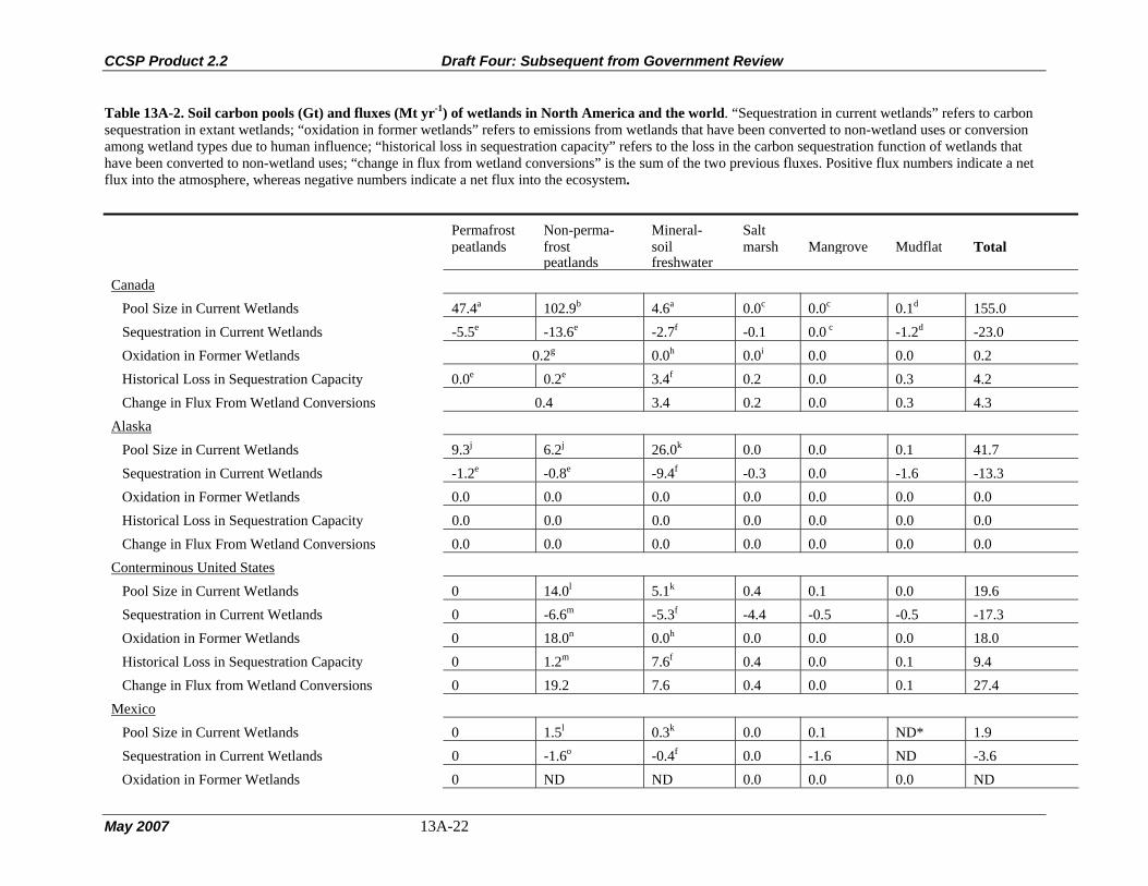
CCSP Product 2.2 Draft Four: Subsequent from Government Review
May 2007 13A-22
Table 13A-2. Soil carbon pools (Gt) and fluxes (Mt yr-1) of wetlands in North America and the world. “Sequestration in current wetlands” refers to carbon sequestration in extant wetlands; “oxidation in former wetlands” refers to emissions from wetlands that have been converted to non-wetland uses or conversion among wetland types due to human influence; “historical loss in sequestration capacity” refers to the loss in the carbon sequestration function of wetlands that have been converted to non-wetland uses; “change in flux from wetland conversions” is the sum of the two previous fluxes. Positive flux numbers indicate a net flux into the atmosphere, whereas negative numbers indicate a net flux into the ecosystem.
Permafrost Non-perma- Mineral- Salt peatlands frost soil marsh Mangrove Mudflat Total peatlands freshwaterCanada Pool Size in Current Wetlands 47.4a 102.9b 4.6a 0.0c 0.0c 0.1d 155.0 Sequestration in Current Wetlands -5.5e -13.6e -2.7f -0.1 0.0 c -1.2d -23.0 Oxidation in Former Wetlands 0.2g 0.0h 0.0i 0.0 0.0 0.2 Historical Loss in Sequestration Capacity 0.0e 0.2e 3.4f 0.2 0.0 0.3 4.2 Change in Flux From Wetland Conversions 0.4 3.4 0.2 0.0 0.3 4.3 Alaska Pool Size in Current Wetlands 9.3j 6.2j 26.0k 0.0 0.0 0.1 41.7 Sequestration in Current Wetlands -1.2e -0.8e -9.4f -0.3 0.0 -1.6 -13.3 Oxidation in Former Wetlands 0.0 0.0 0.0 0.0 0.0 0.0 0.0 Historical Loss in Sequestration Capacity 0.0 0.0 0.0 0.0 0.0 0.0 0.0 Change in Flux From Wetland Conversions 0.0 0.0 0.0 0.0 0.0 0.0 0.0 Conterminous United States Pool Size in Current Wetlands 0 14.0l 5.1k 0.4 0.1 0.0 19.6 Sequestration in Current Wetlands 0 -6.6m -5.3f -4.4 -0.5 -0.5 -17.3 Oxidation in Former Wetlands 0 18.0n 0.0h 0.0 0.0 0.0 18.0 Historical Loss in Sequestration Capacity 0 1.2m 7.6f 0.4 0.0 0.1 9.4 Change in Flux from Wetland Conversions 0 19.2 7.6 0.4 0.0 0.1 27.4 Mexico Pool Size in Current Wetlands 0 1.5l 0.3k 0.0 0.1 ND* 1.9 Sequestration in Current Wetlands 0 -1.6o -0.4f 0.0 -1.6 ND -3.6 Oxidation in Former Wetlands 0 ND ND 0.0 0.0 0.0 ND

CCSP Product 2.2 Draft Four: Subsequent from Government Review
May 2007 13A-23
Historical Loss in Sequestration Capacity 0 ND ND 0.0 1.0 ND ND Change in Flux from Wetland Conversions 0 ND ND 0.0 1.0 ND ND North America Pool Size in Current Wetlands 56.7 124.6 36.0 0.4 0.2 0.3 218.2 Sequestration in Current Wetlands -6.6 -22.6 -17.7 -4.8 -2.1 -3.3 -57.2 Oxidation in Former Wetlands 18.2 0.0 0.0 0.0 0.0 18.2 Historical Loss in Sequestration Capacity 0 1.4 11.0 0.5 1.0 0.5 14.5 Change in Flux from Wetland Conversions 19.6 11.0 0.5 1.0 0.5 32.7 Global Pool Size in Current Wetlands 462p 46q 0.4r 4.9r ND 513 Sequestration in Current Wetlands -55s -39f -4.6r -38.0r ND -137 Oxidation in Former Wetlands 205t ND 0 0 0 205 Historical Loss in Sequestration Capacity 16t 45f 0.7u 20v ND 82 Change in Flux From Wetland Conversions 221t > 45 0.7 20 ND 287
*ND indicates that no data are available. aTarnocai. (1998); mineral soil to 1-m depth. bTarnocai et al. (2005). c Rates and pools calculated from Chmura et al. (2003) using country-specific data (sedimentation accumulation rates in Mg C ha-1 yr-1: Mexican mangroves
= 3.3, conterminous U.S. mangroves = 1.8. conterminous tidal marshes = 2.2, tidal marshes in Canada and Alaska = 2.1); areas from Table 13A-1... dAssumed the same carbon density and accumulation rates as the adjacent vegetated wetland ecosystem (mangrove data for Mexico and salt marsh data
elsewhere). eAssumed carbon accumulation rate of 0.13 Mg C ha-1 yr-1 for permafrost peatlands and 0.19 Mg C ha-1 yr-1 for non-permafrost peatlands. Reported range of
long-term apparent accumulation rates from 0.05-0.35 (Ovenden, 1990; Maltby and Immirzi, 1993; Trumbore and Harden, 1997; Vitt et al., 2000; Turunen et al.,
2004). fRate calculated as the geometric mean sediment accumulation rate of 2.2 Mg sediment ha-1 yr-1 (range 0-80) from Johnston (1991) and Craft and Casey
(2000) times 7.7 % C (CV = 109) (Batjes 1996). gSum of 0.24 Mt C yr-1 from horticulture removal of peat (Cleary et al., 2005) and 0.10 Mt C yr-1 from increased peat sequestration due to permafrost melting
(Turetsky et al., 2002).

CCSP Product 2.2 Draft Four: Subsequent from Government Review
May 2007 13A-24
hAssumed that the net oxidation of 8.6% of the soil carbon pool (Euliss et al., 2006) over 50 yr after conversion to non-wetland use. iAssumed that conversion of tidal systems is caused by fill and results in burial and preservation of SOM define SOM rather than oxidation. jSoil carbon densities of 1,441 Mg C ha-1 for Histosols and 1,048 Mg C ha-1 for Histels (Tarnocai et al., 2005). kSoil carbon density of 162 Mg C ha-1 for the conterminous United States and Mexico and 468 Mg C ha-1 for Alaska based upon NRCS STATSGO database
and soil pedon information. lAssumed soil carbon density of 1,500 Mg C ha-1. mWebb and Webb (1988). nEstimated loss rate as of early 1980s (Armentano and Menges,1986). Overall wetlands losses in the United States have declined dramatically since then
(Dahl, 2000) and probably even more so for Histosols, so this number may still be representative. oUsing peat accumulation rate of 1.6 Mg C ha-1 (range 1.0–2.25) (Maltby and Immirzi, 1993). pFrom Maltby and Immirzi (1993). Range of 234 to 679 Gt C (Gorham, 1991; Maltby and Immirzi, 1993; Eswaran et al., 1995; Batjes, 1996; Lappalainen,
1996; Joosten and Clarke, 2002). qSoil carbon density of 199 Mg C ha-1 (Batjes, 1996). rChmura et al. (2003). sJoosten and Clarke (2002) reported range of -40 to -70 Mt C yr-1 . Using the peatland estimate in Table 13A-1 and a C accumulation rate of 0.19 Mg C ha-1
yr-1, we calculate a global flux of -65 Mt C yr-1 in peatlands. tCurrent oxidative flux is the difference between the change in flux and the historical loss in sequestration capacity from this table. The change in flux is from
Maltby and Immirzi (1993) (reported range 176 to 266 Mt C yr-1) and the historical loss in sequestration capacity is from this table for North America, from
Armentano and Menges (1986) for other northern peatlands, and from Maltby and Immirzi (1993) for tropical peatlands. uAssumed that global rates approximate the North America rate because most salt marshes inventoried are in North America. vAssumed 25% loss globally since the late 1800s.

CCSP Product 2.2 Draft Four: Subsequent from Government Review
May 2007 13A-25
Table 13A-3. Plant carbon pools (Gt) and fluxes (Mt yr-1) of wetlands in North America and the world. Positive flux numbers indicate a net
flux into the atmosphere, whereas negative numbers indicate a net flux into the ecosystem.
Permafrost Non-perma- Mineral- Salt peatlands frost soil marsh Mangrove Total peatlands freshwater Canada Pool Size in Current Wetlands 1.4a 0.3b 0.0c 0.0 1.7 Sequestration in Current Wetlands 0.0 ND* 0.0 0.0 0.0 Alaska Pool Size in Current Wetlands 0.4a 1.1d 0.0 0.0 1.5 Sequestration in Current Wetlands 0.0 0.0 0.0 0.0 0.0 0.0 Conterminous United States Pool Size in Current Wetlands 0.0 1.5d 0.0 0.0 1.5 Sequestration in Current Wetlands 0.0 -10.3e 0.0 0.0 -10.3 Mexico Pool Size in Current Wetlands 0.0 0.0b 0.0b 0.0 0.1 0.1 Sequestration in Current Wetlands 0.0 ND ND 0.0 ND 0.0 North America Pool Size in Current Wetlands 4.8 0.0 0.1 4.9 Sequestration in Current Wetlands 0.0 -10.3 0.0 ND -10.3 Global Pool Size in Current Wetlands 6.9b 4.6b 0.0f 4.0g 15.5 Sequestration in Current Wetlands 0.0 ND ND 0.0 ND ND
*ND indicates that no data are available. aBiomass for non-forested peatlands from Vitt et al. (2000), assuming 50% of biomass is belowground. Forest biomass density from
Birdsey (1992) and forested area from Tarnocai et al. (2005) for Canada and from Hall et al. (1994) for Alaska. bAssumed 2000 g C m-2 in aboveground and belowground plant biomass (Gorham, 1991). cBiomass data from Mitsch and Gosselink (1993). dBiomass for non-forested wetlands from Gorham (1991). Forest biomass density from Birdsey (1992), and forested area from Hall et al. (1994) for Alaska and Dahl (2000) for the conterminous U.S.. e50 g C m-2 yr-1 sequestration from forest growth from a southeastern U.S. regional assessment of wetland forest growth (Brown et al., 2001). fAssumed that global pools approximate those from North America because most salt marshes inventoried are in North America. gTwilley et al. (1992).
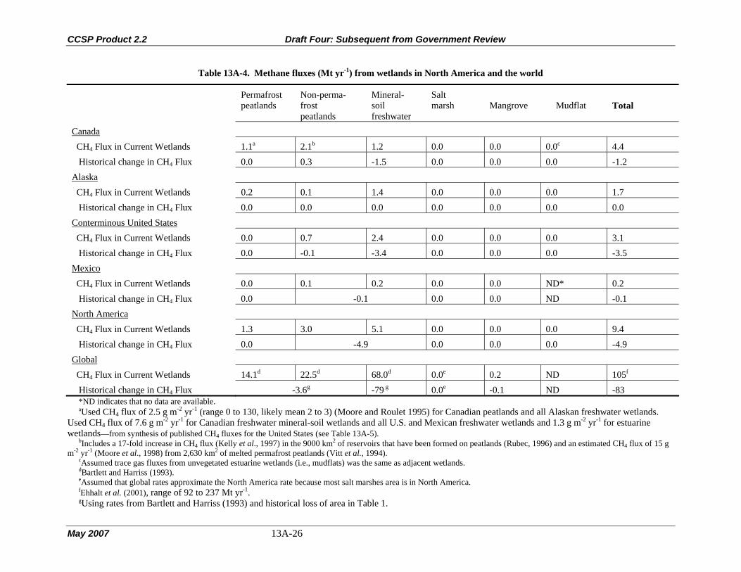
CCSP Product 2.2 Draft Four: Subsequent from Government Review
May 2007 13A-26
Table 13A-4. Methane fluxes (Mt yr-1) from wetlands in North America and the world
Permafrost Non-perma- Mineral- Salt peatlands frost soil marsh Mangrove Mudflat Total peatlands freshwater Canada CH4 Flux in Current Wetlands 1.1a 2.1b 1.2 0.0 0.0 0.0c 4.4 Historical change in CH4 Flux 0.0 0.3 -1.5 0.0 0.0 0.0 -1.2 Alaska CH4 Flux in Current Wetlands 0.2 0.1 1.4 0.0 0.0 0.0 1.7 Historical change in CH4 Flux 0.0 0.0 0.0 0.0 0.0 0.0 0.0 Conterminous United States CH4 Flux in Current Wetlands 0.0 0.7 2.4 0.0 0.0 0.0 3.1 Historical change in CH4 Flux 0.0 -0.1 -3.4 0.0 0.0 0.0 -3.5 Mexico CH4 Flux in Current Wetlands 0.0 0.1 0.2 0.0 0.0 ND* 0.2 Historical change in CH4 Flux 0.0 -0.1 0.0 0.0 ND -0.1 North America CH4 Flux in Current Wetlands 1.3 3.0 5.1 0.0 0.0 0.0 9.4 Historical change in CH4 Flux 0.0 -4.9 0.0 0.0 0.0 -4.9 Global CH4 Flux in Current Wetlands 14.1d 22.5d 68.0d 0.0e 0.2 ND 105f Historical change in CH4 Flux -3.6g -79 g 0.0e -0.1 ND -83
*ND indicates that no data are available. aUsed CH4 flux of 2.5 g m-2 yr-1 (range 0 to 130, likely mean 2 to 3) (Moore and Roulet 1995) for Canadian peatlands and all Alaskan freshwater wetlands.
Used CH4 flux of 7.6 g m-2 yr-1 for Canadian freshwater mineral-soil wetlands and all U.S. and Mexican freshwater wetlands and 1.3 g m-2 yr-1 for estuarine wetlands—from synthesis of published CH4 fluxes for the United States (see Table 13A-5).
bIncludes a 17-fold increase in CH4 flux (Kelly et al., 1997) in the 9000 km2 of reservoirs that have been formed on peatlands (Rubec, 1996) and an estimated CH4 flux of 15 g m-2 yr-1 (Moore et al., 1998) from 2,630 km2 of melted permafrost peatlands (Vitt et al., 1994).
cAssumed trace gas fluxes from unvegetated estuarine wetlands (i.e., mudflats) was the same as adjacent wetlands. dBartlett and Harriss (1993). eAssumed that global rates approximate the North America rate because most salt marshes area is in North America. fEhhalt et al. (2001), range of 92 to 237 Mt yr-1. gUsing rates from Bartlett and Harriss (1993) and historical loss of area in Table 1.

CCSP Product 2.2 Draft Four: Subsequent from Government Review
May 2007 13A-27
Table 13A-5. Methane fluxes measured in the conterminous United States. The conversion factor is the ratio of the daily average flux to the measured annual 1 flux × 103. The calculated annual flux was determined based upon the average conversion factor for freshwater (FW) and saltwater wetlands (SW). The measured 2
annual flux was used if that was available; otherwise, the calculated annual flux was used. 3 4 Daily Measured Conversion Estimated Used Salt/ Average Annual Factor Annual Annual Habitat State Methoda Fresh Flux Flux Flux Flux Reference
(mg CH4 m-2 d-1)
(g CH4 m-2 yr-1)
(g CH4 m-2 yr-1)
(g CH4 m-2 yr-1)
Fens CO C FW 40.7 40.7 Chimner and Cooper (2003) Wet Alpine Meadow CO C FW 0.1 0.0 0.0 Neff et al. (1994) Lake - Average CO C FW 25.4 9.2 9.2 Smith and Lewis (1992) Wetland - Average CO C FW 28.3 10.3 10.3 Smith and Lewis (1992) Nuphar Bed CO C FW 202.1 73.6 73.6 Smith and Lewis (1992) Tundra - Carex Meadow CO C FW 2.8 1.0 1.0 West et al. (1999) Tundra - Acomastylis Meadow CO C FW -0.5 -0.2 -0.2 West et al. (1999) Tundra - Kobresia Meadow CO C FW -0.8 -0.3 -0.3 West et al. (1999) Moist Grassy CO C FW 6.1 1.9 0.32 2.2 1.9 Wickland et al. (1999) Moist Mossy CO C FW 1.5 0.5 0.33 0.5 0.5 Wickland et al. (1999) Wetland CO C FW 41.7 41.7 Wickland et al. (1999) Hardwood Hammock FL C FW 0.0 0.0 0.0 Bartlett et al. (1989) Dwarf Cypress / Sawgrass FL C FW 7.5 2.7 2.7 Bartlett et al. (1989) Spikerush FL C FW 29.4 10.7 10.7 Bartlett et al. (1989) Sawgrass < 1m FL C FW 38.8 14.1 14.1 Bartlett et al. (1989) Sawgrass/Spkerush/Periphyton FL C FW 45.1 16.4 16.4 Bartlett et al. (1989) Swamp Forest FL C FW 68.9 25.1 25.1 Bartlett et al. (1989) Sawgrass > 1m FL C FW 71.9 26.2 26.2 Bartlett et al. (1989) Sawgrass FL C FW 107.0 38.9 38.9 Burke et al. (1988) Pond Open Water FL C FW 624.0 227.1 227.1 Burke et al. (1988) Everglades - Cladium FL C FW 45.4 16.5 16.5 Chanton et al. (1993) Everglades - Typha FL C FW 142.9 52.0 52.0 Chanton et al. (1993) Wet Prairie (Marl) FL C FW 87.0 31.6 31.6 Happell et al. (1993) Wet Prairie (Marl) FL C FW 27.4 10.0 10.0 Happell et al. (1993) Marsh (Marl) FL C FW 30.0 10.9 10.9 Happell et al. (1993) Marsh (Marl) FL C FW 49.6 18.0 18.0 Happell et al. (1993) Marsh (Peat) FL C FW 45.4 16.5 16.5 Happell et al. (1993)
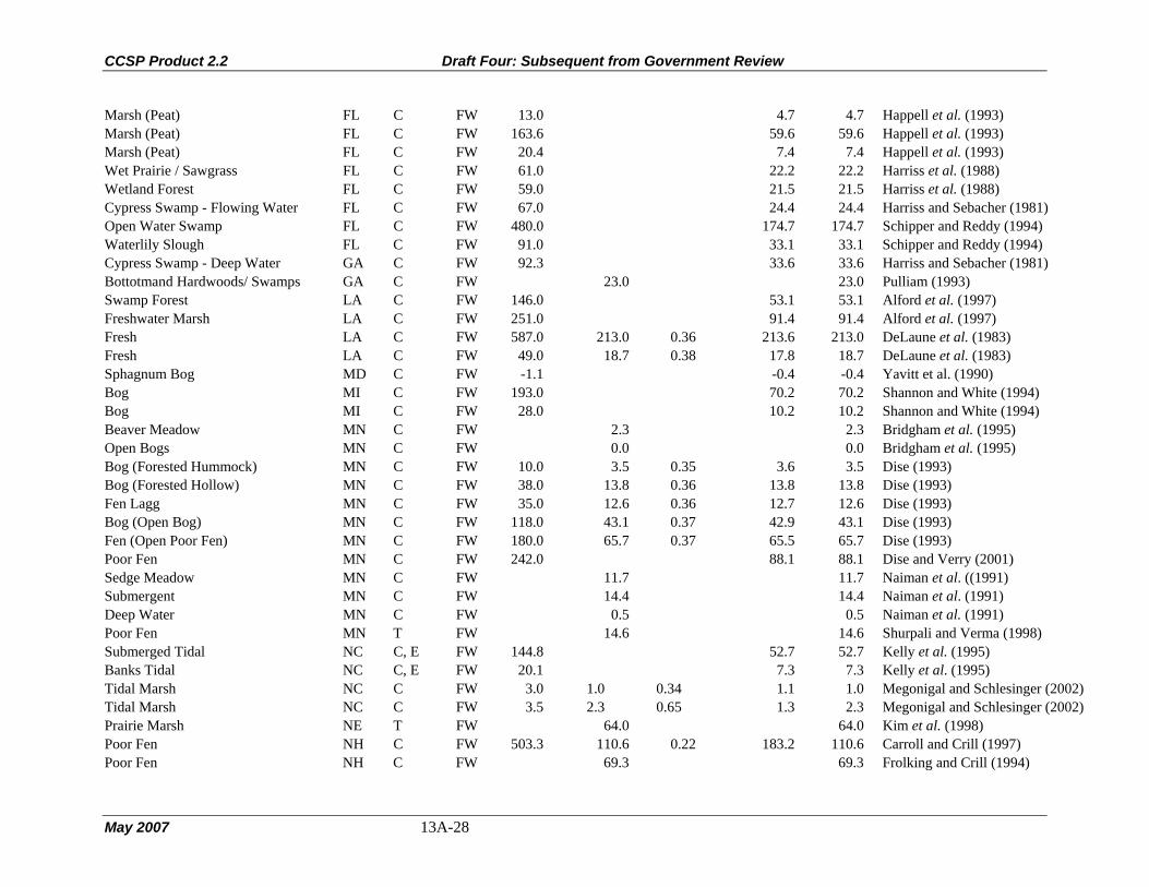
CCSP Product 2.2 Draft Four: Subsequent from Government Review
May 2007 13A-28
Marsh (Peat) FL C FW 13.0 4.7 4.7 Happell et al. (1993) Marsh (Peat) FL C FW 163.6 59.6 59.6 Happell et al. (1993) Marsh (Peat) FL C FW 20.4 7.4 7.4 Happell et al. (1993) Wet Prairie / Sawgrass FL C FW 61.0 22.2 22.2 Harriss et al. (1988) Wetland Forest FL C FW 59.0 21.5 21.5 Harriss et al. (1988) Cypress Swamp - Flowing Water FL C FW 67.0 24.4 24.4 Harriss and Sebacher (1981) Open Water Swamp FL C FW 480.0 174.7 174.7 Schipper and Reddy (1994) Waterlily Slough FL C FW 91.0 33.1 33.1 Schipper and Reddy (1994) Cypress Swamp - Deep Water GA C FW 92.3 33.6 33.6 Harriss and Sebacher (1981) Bottotmand Hardwoods/ Swamps GA C FW 23.0 23.0 Pulliam (1993) Swamp Forest LA C FW 146.0 53.1 53.1 Alford et al. (1997) Freshwater Marsh LA C FW 251.0 91.4 91.4 Alford et al. (1997) Fresh LA C FW 587.0 213.0 0.36 213.6 213.0 DeLaune et al. (1983) Fresh LA C FW 49.0 18.7 0.38 17.8 18.7 DeLaune et al. (1983) Sphagnum Bog MD C FW -1.1 -0.4 -0.4 Yavitt et al. (1990) Bog MI C FW 193.0 70.2 70.2 Shannon and White (1994) Bog MI C FW 28.0 10.2 10.2 Shannon and White (1994) Beaver Meadow MN C FW 2.3 2.3 Bridgham et al. (1995) Open Bogs MN C FW 0.0 0.0 Bridgham et al. (1995) Bog (Forested Hummock) MN C FW 10.0 3.5 0.35 3.6 3.5 Dise (1993) Bog (Forested Hollow) MN C FW 38.0 13.8 0.36 13.8 13.8 Dise (1993) Fen Lagg MN C FW 35.0 12.6 0.36 12.7 12.6 Dise (1993) Bog (Open Bog) MN C FW 118.0 43.1 0.37 42.9 43.1 Dise (1993) Fen (Open Poor Fen) MN C FW 180.0 65.7 0.37 65.5 65.7 Dise (1993) Poor Fen MN C FW 242.0 88.1 88.1 Dise and Verry (2001) Sedge Meadow MN C FW 11.7 11.7 Naiman et al. ((1991) Submergent MN C FW 14.4 14.4 Naiman et al. (1991) Deep Water MN C FW 0.5 0.5 Naiman et al. (1991) Poor Fen MN T FW 14.6 14.6 Shurpali and Verma (1998) Submerged Tidal NC C, E FW 144.8 52.7 52.7 Kelly et al. (1995) Banks Tidal NC C, E FW 20.1 7.3 7.3 Kelly et al. (1995) Tidal Marsh NC C FW 3.0 1.0 0.34 1.1 1.0 Megonigal and Schlesinger (2002) Tidal Marsh NC C FW 3.5 2.3 0.65 1.3 2.3 Megonigal and Schlesinger (2002) Prairie Marsh NE T FW 64.0 64.0 Kim et al. (1998) Poor Fen NH C FW 503.3 110.6 0.22 183.2 110.6 Carroll and Crill (1997) Poor Fen NH C FW 69.3 69.3 Frolking and Crill (1994)
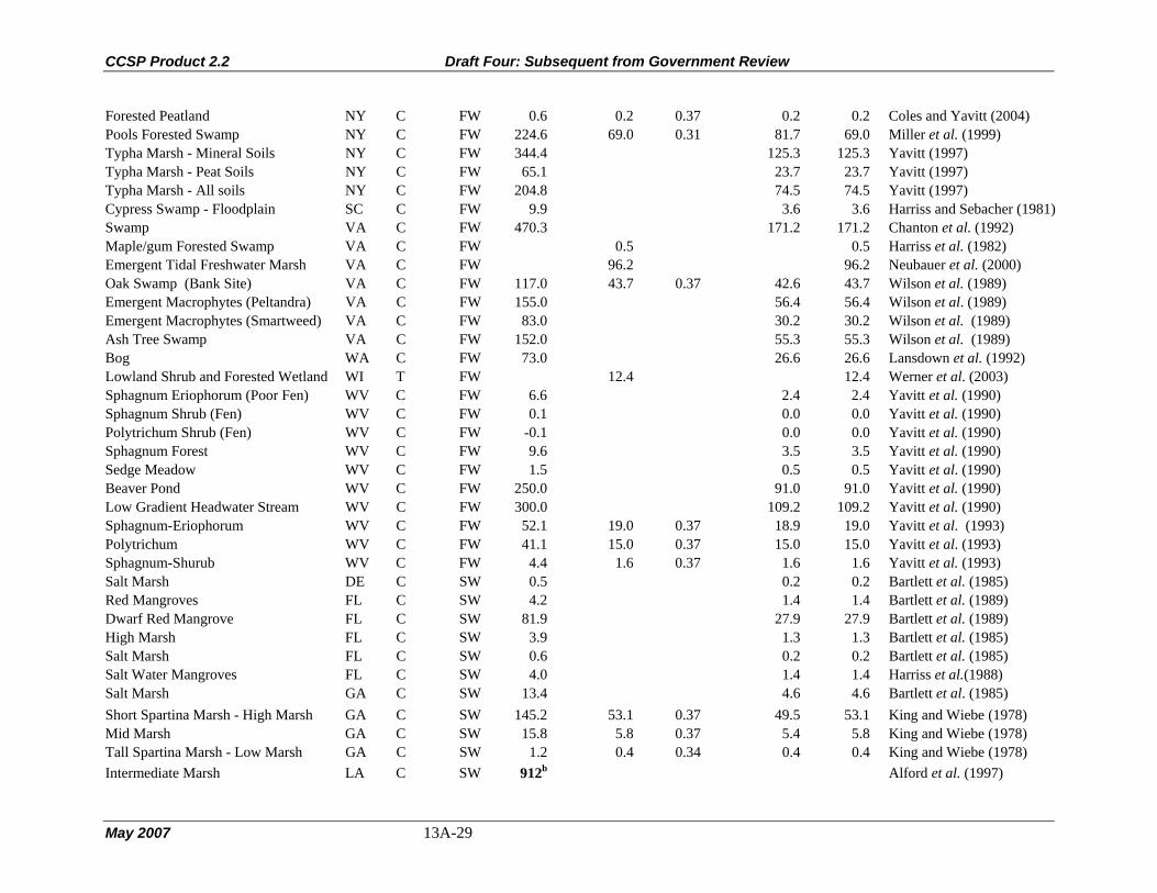
CCSP Product 2.2 Draft Four: Subsequent from Government Review
May 2007 13A-29
Forested Peatland NY C FW 0.6 0.2 0.37 0.2 0.2 Coles and Yavitt (2004) Pools Forested Swamp NY C FW 224.6 69.0 0.31 81.7 69.0 Miller et al. (1999) Typha Marsh - Mineral Soils NY C FW 344.4 125.3 125.3 Yavitt (1997) Typha Marsh - Peat Soils NY C FW 65.1 23.7 23.7 Yavitt (1997) Typha Marsh - All soils NY C FW 204.8 74.5 74.5 Yavitt (1997) Cypress Swamp - Floodplain SC C FW 9.9 3.6 3.6 Harriss and Sebacher (1981) Swamp VA C FW 470.3 171.2 171.2 Chanton et al. (1992) Maple/gum Forested Swamp VA C FW 0.5 0.5 Harriss et al. (1982) Emergent Tidal Freshwater Marsh VA C FW 96.2 96.2 Neubauer et al. (2000) Oak Swamp (Bank Site) VA C FW 117.0 43.7 0.37 42.6 43.7 Wilson et al. (1989) Emergent Macrophytes (Peltandra) VA C FW 155.0 56.4 56.4 Wilson et al. (1989) Emergent Macrophytes (Smartweed) VA C FW 83.0 30.2 30.2 Wilson et al. (1989) Ash Tree Swamp VA C FW 152.0 55.3 55.3 Wilson et al. (1989) Bog WA C FW 73.0 26.6 26.6 Lansdown et al. (1992) Lowland Shrub and Forested Wetland WI T FW 12.4 12.4 Werner et al. (2003) Sphagnum Eriophorum (Poor Fen) WV C FW 6.6 2.4 2.4 Yavitt et al. (1990) Sphagnum Shrub (Fen) WV C FW 0.1 0.0 0.0 Yavitt et al. (1990) Polytrichum Shrub (Fen) WV C FW -0.1 0.0 0.0 Yavitt et al. (1990) Sphagnum Forest WV C FW 9.6 3.5 3.5 Yavitt et al. (1990) Sedge Meadow WV C FW 1.5 0.5 0.5 Yavitt et al. (1990) Beaver Pond WV C FW 250.0 91.0 91.0 Yavitt et al. (1990) Low Gradient Headwater Stream WV C FW 300.0 109.2 109.2 Yavitt et al. (1990) Sphagnum-Eriophorum WV C FW 52.1 19.0 0.37 18.9 19.0 Yavitt et al. (1993) Polytrichum WV C FW 41.1 15.0 0.37 15.0 15.0 Yavitt et al. (1993) Sphagnum-Shurub WV C FW 4.4 1.6 0.37 1.6 1.6 Yavitt et al. (1993) Salt Marsh DE C SW 0.5 0.2 0.2 Bartlett et al. (1985) Red Mangroves FL C SW 4.2 1.4 1.4 Bartlett et al. (1989) Dwarf Red Mangrove FL C SW 81.9 27.9 27.9 Bartlett et al. (1989) High Marsh FL C SW 3.9 1.3 1.3 Bartlett et al. (1985) Salt Marsh FL C SW 0.6 0.2 0.2 Bartlett et al. (1985) Salt Water Mangroves FL C SW 4.0 1.4 1.4 Harriss et al.(1988) Salt Marsh GA C SW 13.4 4.6 4.6 Bartlett et al. (1985) Short Spartina Marsh - High Marsh GA C SW 145.2 53.1 0.37 49.5 53.1 King and Wiebe (1978) Mid Marsh GA C SW 15.8 5.8 0.37 5.4 5.8 King and Wiebe (1978) Tall Spartina Marsh - Low Marsh GA C SW 1.2 0.4 0.34 0.4 0.4 King and Wiebe (1978) Intermediate Marsh LA C SW 912b Alford et al. (1997)

CCSP Product 2.2 Draft Four: Subsequent from Government Review
May 2007 13A-30
Salt Marsh LA C SW 15.7 5.7 0.36 5.4 5.7 DeLaune et al. (1983) Brackish LA C SW 267.0 97.0 91.1 97.0 DeLaune et al. (1983) Salt Marsh LA C SW 4.8 1.7 0.35 1.6 1.7 DeLaune et al. (1983) Brackish LA C SW 17.0 6.4 0.38 5.8 6.4 DeLaune et al. (1983) Cypress Swamp - Floodplain SC C SW 1.5 0.5 0.5 Bartlett et al. (1985) Salt Marsh SC C SW 0.4 0.1 0.1 Bartlett et al. (1985) Salt Marsh VA C SW 3.0 1.3 0.43 1.0 1.3 Bartlett et al. (1985) Salt Marsh VA C SW 5.0 1.2 0.24 1.7 1.2 Bartlett et al. (1985) Salt Meadow VA C SW 2.0 0.4 0.22 0.7 0.4 Bartlett et al. (1985) Salt Marsh VA C SW -0.8 -0.3 -0.3 Bartlett et al. (1985) Salt Marsh VA C SW 1.5 0.5 0.5 Bartlett et al. (1985) Salt Meadow VA C SW -1.9 -0.6 -0.6 Bartlett et al. (1985) Tidal Salt Marsh VA C SW 16.0 5.6 0.35 5.5 5.6 Bartlett et al. (1987) Tidal Brackish Marsh VA C SW 64.6 22.4 0.35 22.0 22.4 Bartlett et al. (1987) Tidal Brackish/Fresh Marsh VA C SW 53.5 18.2 0.34 18.2 18.2 Bartlett et al. (1987) Freshwater n 32 18 74 88 Arithmetic Mean 32.1 0.36 38.6 36.0 Arithmetic Standard Error 7.9 0.02 6.0 5.0 Geometric Mean 8.1 7.1 7.6 Geometric Standard Error 2.1 0.82 2.2 Saltwater n 13 12 25 25 Arithmetic Mean 16.9 0.34 9.8 10.3 Arithmetic Standard Error 7.8 0.02 4.1 4.4 Geometric Mean 5.0 1.3 1.3 Geometric Standard Error 2.0 0.2 3.3 1
aC = chamber, T = tower, eddy covariance, E = ebulition measured separately. 2 bOutlier that was removed from further analysis. 3

CCSP Product 2.2 Draft Four: Subsequent from Government Review
May 2007 15A-1
APPENDIX 15A
New pCO2 Database for Coastal Ocean Waters Surrounding North America
A database for the partial pressure of CO2 (pCO2), temperature, and salinity in surface waters within
about 1,000 km from the shore of the North American continent has been assembled. About 550,000
seawater pCO2 observations were made from 1979 to 2004 by the authors and collaborators of Chapter
15. The pCO2 data have been obtained by a method using an infrared gas analyzer or gas-chromatograph
for the determination of CO2 concentrations in a carrier gas equilibrated with seawater at a known
temperature and total pressure. The precision of pCO2 measurements has been estimated to be about ±
0.7% on average. The quality-controlled data are archived at www.ldeo.columbia.edu/res/pi/CO2.
The zonal distribution of the surface water pCO2, sea surface temperature (SST), and salinity data
shows that the greatest variability is confined within 300 km from the shores of both the Atlantic and
Pacific. Observations made in various years were combined into a single year and were averaged into 1°
× 1° pixels (approximately N-S 100 km by E-W 80 km) for the analysis. Accordingly, the results
represent a climatological mean condition over the past 25 years. Finer resolutions (10 × 10 km) may be
desirable for some areas close to shore because of outflow of estuarine and river waters and upwelling.
However, for this study, which is aimed at a broad picture of waters surrounding the continent, the fine
scale measurements have been incorporated into the 1° × 1° pixels. In addition, data with salinities of less
than 16.0 are considered to be inland waters and have been excluded from the analysis.
Climatological monthly and annual mean values for pCO2 in each zone where computed first. Then
the air-sea pCO2 difference, which represents the thermodynamic driving potential for air-sea CO2 gas
transfer, was estimated using the atmospheric CO2 concentration data. Finally, the net air-sea CO2 flux
was computed using transfer coefficients estimated on the basis of climatological mean monthly wind
speeds using the (wind speed)2 formulation of Wanninkhof (1992). The transfer coefficient depends on
the state of turbulence above and below the air-sea interface and is commonly parameterized as a function
of wind speeds (corrected to 10 m above the sea surface). However, selection of wind data is problematic
because wind speeds vary with the time scale (hourly, diurnal, or seasonal). For example, fluxes
calculated for the South Atlantic Bight from 6-h mean wind speeds in the NCEP/NCAR version 2 file (1°
× 1° mean) were lower than those estimated using the monthly mean. This discrepancy suggests that ships
used commonly for coastal carbon studies tend to be small and hence are rarely at sea under high wind
conditions, so observations are biased toward lower winds. Taking into account that the observations have

CCSP Product 2.2 Draft Four: Subsequent from Government Review
May 2007 15A-2
been made infrequently over multiple years, the gas transfer coefficients estimated from climatological
mean monthly wind speeds may be more representative. The Schmidt number is computed using
measured SST and climatological mean salinity (DaSilva et al. 1994). The flux values in a given month
are then averaged to yield a climatological mean flux (and standard deviation) for each month. This
procedure assumes implicitly that the seawater pCO2 changes at much slower rates in space and time than
the wind speed and that the seawater pCO2 does not correlate with the wind speed.
REFERENCES DaSilva, A., C. Young, and S. Levitus, 1994: Atlas of Marine Surface Data 1994. NOAA Atlas NESDIS 6, U.S.
Department of Commerce, Washington, DC.
Wanninkhof, R., 1992: Relationship between wind speed and gas exchange. Journal of Geophysical Research, 97,
7373-7382.

[Inside Back Cover]
Climate Change Science Program and the Subcommittee on Global Change Research
William J. Brennan, Chair Department of Commerce National Oceanic and Atmospheric Administration Acting Director, Climate Change Science Program Jack Kaye, Vice Chair National Aeronautics and Space Administration Allen Dearry Department of Health and Human Services Jerry Elwood Department of Energy Mary Glackin National Oceanic and Atmospheric Administration Patricia Gruber Department of Defense William Hohenstein Department of Agriculture Linda Lawson Department of Transportation Mark Myers U.S. Geological Survey Jarvis Moyers National Science Foundation Patrick Neale Smithsonian Institution Jacqueline Schafer U.S. Agency for International Development Joel Scheraga Environmental Protection Agency Harlan Watson Department of State
Executive Office and other Liaisons Melissa Brandt Office of Management and Budget Stephen Eule Department of Energy Director, Climate Change Technology Program Katharine Gebbie National Institute of Standards & Technology Margaret McCalla Office of the Federal Coordinator for Meteorology Bob Rainey Council on Environmental Quality Gene Whitney Office of Science and Technology Policy

[This page intentionally left blank]