global carbon budget 2018 - vliz
TRANSCRIPT

Earth Syst. Sci. Data, 10, 2141–2194, 2018https://doi.org/10.5194/essd-10-2141-2018© Author(s) 2018. This work is distributed underthe Creative Commons Attribution 4.0 License.
Global Carbon Budget 2018
Corinne Le Quéré1, Robbie M. Andrew2, Pierre Friedlingstein3, Stephen Sitch4, Judith Hauck5,Julia Pongratz6,7, Penelope A. Pickers8, Jan Ivar Korsbakken2, Glen P. Peters2, Josep G. Canadell9,
Almut Arneth10, Vivek K. Arora11, Leticia Barbero12,13, Ana Bastos6, Laurent Bopp14,Frédéric Chevallier15, Louise P. Chini16, Philippe Ciais15, Scott C. Doney17, Thanos Gkritzalis18,
Daniel S. Goll15, Ian Harris19, Vanessa Haverd20, Forrest M. Hoffman21, Mario Hoppema5,Richard A. Houghton22, George Hurtt16, Tatiana Ilyina7, Atul K. Jain23, Truls Johannessen24,
Chris D. Jones25, Etsushi Kato26, Ralph F. Keeling27, Kees Klein Goldewijk28,29, Peter Landschützer7,Nathalie Lefèvre30, Sebastian Lienert31, Zhu Liu1,54, Danica Lombardozzi32, Nicolas Metzl30,David R. Munro33, Julia E. M. S. Nabel7, Shin-ichiro Nakaoka34, Craig Neill35,36, Are Olsen24,
Tsueno Ono38, Prabir Patra39, Anna Peregon15, Wouter Peters40,41, Philippe Peylin15,Benjamin Pfeil24,37, Denis Pierrot12,13, Benjamin Poulter42, Gregor Rehder43, Laure Resplandy44,Eddy Robertson25, Matthias Rocher45, Christian Rödenbeck46, Ute Schuster4, Jörg Schwinger37,
Roland Séférian45, Ingunn Skjelvan37, Tobias Steinhoff47, Adrienne Sutton48, Pieter P. Tans49,Hanqin Tian50, Bronte Tilbrook35,36, Francesco N. Tubiello51, Ingrid T. van der Laan-Luijkx40,
Guido R. van der Werf52, Nicolas Viovy15, Anthony P. Walker53, Andrew J. Wiltshire25,Rebecca Wright1,8, Sönke Zaehle46, and Bo Zheng15
1Tyndall Centre for Climate Change Research, University of East Anglia,Norwich Research Park, Norwich NR4 7TJ, UK
2CICERO Center for International Climate Research, Oslo 0349, Norway3College of Engineering, Mathematics and Physical Sciences, University of Exeter, Exeter EX4 4QF, UK
4College of Life and Environmental Sciences, University of Exeter, Exeter EX4 4RJ, UK5Alfred Wegener Institute Helmholtz Centre for Polar and Marine Research,
Postfach 120161, 27515 Bremerhaven, Germany6Ludwig-Maximilians-Universität Munich, Luisenstr. 37, 80333 Munich, Germany
7Max Planck Institute for Meteorology, Hamburg, Germany8Centre for Ocean and Atmospheric Sciences, School of Environmental Sciences,
University of East Anglia, Norwich Research Park, Norwich NR4 7TJ, UK9Global Carbon Project, CSIRO Oceans and Atmosphere, GPO Box 1700, Canberra, ACT 2601, Australia
10Karlsruhe Institute of Technology, Institute of Meteorology and Climate Research/AtmosphericEnvironmental Research, 82467 Garmisch-Partenkirchen, Germany
11Canadian Centre for Climate Modelling and Analysis, Climate Research Division,Environment and Climate Change Canada, Victoria, BC, Canada
12Cooperative Institute for Marine and Atmospheric Studies, Rosenstiel Schoolfor Marine and Atmospheric Science, University of Miami, Miami, FL 33149, USA
13National Oceanic & Atmospheric Administration/Atlantic Oceanographic &Meteorological Laboratory (NOAA/AOML), Miami, FL 33149, USA
14Laboratoire de Météorologie Dynamique, Institut Pierre-Simon Laplace, CNRS-ENS-UPMC-X,Département de Géosciences, Ecole Normale Supérieure, 24 rue Lhomond, 75005 Paris, France
15Laboratoire des Sciences du Climat et de l’Environnement, Institut Pierre-Simon Laplace,CEA-CNRS-UVSQ, CE Orme des Merisiers, 91191 Gif-sur-Yvette CEDEX, France
16Department of Geographical Sciences, University of Maryland, College Park, Maryland 20742, USA17University of Virginia, Charlottesville, VA 22904, USA
18Flanders Marine Institute (VLIZ), Wanelaarkaai 7, 8400 Ostend, Belgium
Published by Copernicus Publications.

2142 C. Le Quéré et al.: Global Carbon Budget 2018
19NCAS-Climate, Climatic Research Unit, School of Environmental Sciences,University of East Anglia, Norwich Research Park, Norwich, NR4 7TJ, UK
20CSIRO Oceans and Atmosphere, GPO Box 1700, Canberra, ACT 2601, Australia21Computational Earth Sciences Group, Oak Ridge National Laboratory, Oak Ridge, Tennessee, USA
22Woods Hole Research Center (WHRC), Falmouth, MA 02540, USA23Department of Atmospheric Sciences, University of Illinois, Urbana, IL 61821, USA
24Geophysical Institute, University of Bergen and Bjerknes Centre for Climate Research,Allégaten 70, 5007 Bergen, Norway
25Met Office Hadley Centre, FitzRoy Road, Exeter EX1 3PB, UK26Institute of Applied Energy (IAE), Minato-ku, Tokyo 105-0003, Japan
27University of California, San Diego, Scripps Institution of Oceanography, La Jolla, CA 92093-0244, USA28PBL Netherlands Environmental Assessment Agency, Bezuidenhoutseweg 30,
P.O. Box 30314, 2500 GH, The Hague, the Netherlands29Faculty of Geosciences, Department IMEW, Copernicus Institute of Sustainable Development,
Heidelberglaan 2, P.O. Box 80115, 3508 TC, Utrecht, the Netherlands30Sorbonne Universités (UPMC, Univ Paris 06), CNRS, IRD, MNHN,
LOCEAN/IPSL Laboratory, 75252 Paris, France31Climate and Environmental Physics, Physics Institute and Oeschger Centre
for Climate Change Research, University of Bern, Bern, Switzerland32National Center for Atmospheric Research, Climate and Global Dynamics,
Terrestrial Sciences Section, Boulder, CO 80305, USA33Department of Atmospheric and Oceanic Sciences and Institute of Arctic and Alpine Research,
University of Colorado, Campus Box 450, Boulder, CO 80309-0450, USA34Center for Global Environmental Research, National Institute for Environmental Studies (NIES),
16-2 Onogawa, Tsukuba, Ibaraki 305-8506, Japan35CSIRO Oceans and Atmosphere, P.O. Box 1538, Hobart, Tasmania, 7001, Australia
36Antarctic Climate and Ecosystem Cooperative Research Centre, University of Tasmania, Hobart, Australia37NORCE Norwegian Research Centre and Bjerknes Centre for Climate Research,
Jahnebakken 5, 5007 Bergen, Norway38National Research Institute for Far Sea Fisheries, Japan Fisheries Research and Education Agency,
2-12-4 Fukuura, Kanazawa-Ku, Yokohama 236-8648, Japan39Department of Environmental Geochemical Cycle Research, JAMSTEC, Yokohama, Japan
40Department of Meteorology and Air Quality, Wageningen University & Research,P.O. Box 47, 6700AA Wageningen, the Netherlands
41Centre for Isotope Research, University of Groningen, Nijenborgh 6, 9747 AG Groningen, the Netherlands42NASA Goddard Space Flight Center, Biospheric Sciences Laboratory, Greenbelt, Maryland 20771, USA
43Leibniz Institute for Baltic Sea Research Warnemünde, 18119 Rostock, Germany44Princeton University Department of Geosciences and Princeton Environmental
Institute Princeton, New Jersey, USA45Centre National de Recherche Météorologique, Unite mixte de recherche
3589 Météo-France/CNRS, 42 Avenue Gaspard Coriolis, 31100 Toulouse, France46Max Planck Institute for Biogeochemistry, P.O. Box 600164, Hans-Knöll-Str. 10, 07745 Jena, Germany47GEOMAR Helmholtz Centre for Ocean Research Kiel, Düsternbrooker Weg 20, 24105, Kiel, Germany
48National Oceanic & Atmospheric Administration/Pacific Marine Environmental Laboratory(NOAA/PMEL), 7600 Sand Point Way NE, Seattle, WA 98115, USA
49National Oceanic & Atmospheric Administration, Earth System Research Laboratory(NOAA/ESRL), Boulder, CO 80305, USA
50School of Forestry and Wildlife Sciences, Auburn University, 602 Ducan Drive, Auburn, AL 36849, USA51Statistics Division, Food and Agriculture Organization of the United Nations,
Via Terme di Caracalla, Rome 00153, Italy52Faculty of Science, Vrije Universiteit, Amsterdam, the Netherlands
53Environmental Sciences Division & Climate Change Science Institute,Oak Ridge National Laboratory, Oak Ridge, Tennessee, USA
54Department of Earth System Science, Tsinghua University, Beijing 100084, ChinaCorrespondence: Corinne Le Quéré ([email protected])
Earth Syst. Sci. Data, 10, 2141–2194, 2018 www.earth-syst-sci-data.net/10/2141/2018/

C. Le Quéré et al.: Global Carbon Budget 2018 2143
Received: 27 September 2018 – Discussion started: 4 October 2018Revised: 19 November 2018 – Accepted: 19 November 2018 – Published: 5 December 2018
Abstract. Accurate assessment of anthropogenic carbon dioxide (CO2) emissions and their redistributionamong the atmosphere, ocean, and terrestrial biosphere – the “global carbon budget” – is important to betterunderstand the global carbon cycle, support the development of climate policies, and project future climatechange. Here we describe data sets and methodology to quantify the five major components of the global carbonbudget and their uncertainties. Fossil CO2 emissions (EFF) are based on energy statistics and cement productiondata, while emissions from land use and land-use change (ELUC), mainly deforestation, are based on land useand land-use change data and bookkeeping models. Atmospheric CO2 concentration is measured directly andits growth rate (GATM) is computed from the annual changes in concentration. The ocean CO2 sink (SOCEAN)and terrestrial CO2 sink (SLAND) are estimated with global process models constrained by observations. Theresulting carbon budget imbalance (BIM), the difference between the estimated total emissions and the estimatedchanges in the atmosphere, ocean, and terrestrial biosphere, is a measure of imperfect data and understanding ofthe contemporary carbon cycle. All uncertainties are reported as±1σ . For the last decade available (2008–2017),EFF was 9.4± 0.5 GtC yr−1, ELUC 1.5± 0.7 GtC yr−1, GATM 4.7± 0.02 GtC yr−1, SOCEAN 2.4± 0.5 GtC yr−1,and SLAND 3.2± 0.8 GtC yr−1, with a budget imbalance BIM of 0.5 GtC yr−1 indicating overestimated emis-sions and/or underestimated sinks. For the year 2017 alone, the growth in EFF was about 1.6 % and emissionsincreased to 9.9± 0.5 GtC yr−1. Also for 2017, ELUC was 1.4± 0.7 GtC yr−1, GATM was 4.6± 0.2 GtC yr−1,SOCEAN was 2.5± 0.5 GtC yr−1, and SLAND was 3.8± 0.8 GtC yr−1, with a BIM of 0.3 GtC. The global atmo-spheric CO2 concentration reached 405.0±0.1 ppm averaged over 2017. For 2018, preliminary data for the first6–9 months indicate a renewed growth in EFF of +2.7 % (range of 1.8 % to 3.7 %) based on national emissionprojections for China, the US, the EU, and India and projections of gross domestic product corrected for recentchanges in the carbon intensity of the economy for the rest of the world. The analysis presented here showsthat the mean and trend in the five components of the global carbon budget are consistently estimated over theperiod of 1959–2017, but discrepancies of up to 1 GtC yr−1 persist for the representation of semi-decadal vari-ability in CO2 fluxes. A detailed comparison among individual estimates and the introduction of a broad rangeof observations show (1) no consensus in the mean and trend in land-use change emissions, (2) a persistent lowagreement among the different methods on the magnitude of the land CO2 flux in the northern extra-tropics,and (3) an apparent underestimation of the CO2 variability by ocean models, originating outside the tropics.This living data update documents changes in the methods and data sets used in this new global carbon bud-get and the progress in understanding the global carbon cycle compared with previous publications of this dataset (Le Quéré et al., 2018, 2016, 2015a, b, 2014, 2013). All results presented here can be downloaded fromhttps://doi.org/10.18160/GCP-2018.
1 Introduction
The concentration of carbon dioxide (CO2) in the atmo-sphere has increased from approximately 277 parts per mil-lion (ppm) in 1750 (Joos and Spahni, 2008), the beginning ofthe industrial era, to 405.0± 0.1 ppm in 2017 (Dlugokenckyand Tans, 2018; Fig. 1). The atmospheric CO2 increase abovepre-industrial levels was, initially, primarily caused by therelease of carbon to the atmosphere from deforestation andother land-use change activities (Ciais et al., 2013). Whileemissions from fossil fuels started before the industrial era,they only became the dominant source of anthropogenicemissions to the atmosphere around 1950 and their relativeshare has continued to increase until present. Anthropogenicemissions occur on top of an active natural carbon cycle thatcirculates carbon among the reservoirs of the atmosphere,ocean, and terrestrial biosphere on timescales from sub-daily
to millennial, while exchanges with geologic reservoirs occurat longer timescales (Archer et al., 2009).
The global carbon budget presented here refers to themean, variations, and trends in the perturbation of CO2 inthe environment, referenced to the beginning of the industrialera. It quantifies the input of CO2 to the atmosphere by emis-sions from human activities, the growth rate of atmosphericCO2 concentration, and the resulting changes in the storageof carbon in the land and ocean reservoirs in response to in-creasing atmospheric CO2 levels, climate change, and vari-ability and other anthropogenic and natural changes (Fig. 2).An understanding of this perturbation budget over time andthe underlying variability and trends in the natural carbon cy-cle is necessary to understand the response of natural sinks tochanges in climate, CO2 and land-use change drivers, and thepermissible emissions for a given climate stabilisation target.
www.earth-syst-sci-data.net/10/2141/2018/ Earth Syst. Sci. Data, 10, 2141–2194, 2018

2144 C. Le Quéré et al.: Global Carbon Budget 2018
Figure 1. Surface average atmospheric CO2 concentration (ppm).The 1980–2018 monthly data are from NOAA/ESRL (Dlugokenckyand Tans, 2018) and are based on an average of direct atmosphericCO2 measurements from multiple stations in the marine boundarylayer (Masarie and Tans, 1995). The 1958–1979 monthly data arefrom the Scripps Institution of Oceanography, based on an averageof direct atmospheric CO2 measurements from the Mauna Loa andSouth Pole stations (Keeling et al., 1976). To take into account thedifference of mean CO2 and seasonality between the NOAA/ESRLand the Scripps station networks used here, the Scripps surface av-erage (from two stations) was deseasonalised and harmonised tomatch the NOAA/ESRL surface average (from multiple stations)by adding the mean difference of 0.542 ppm, calculated here fromoverlapping data during 1980–2012.
The components of the CO2 budget that are reported annu-ally in this paper include separate estimates for (1) the CO2emissions from fossil fuel combustion and oxidation fromall energy and industrial processes and cement production(EFF; GtC yr−1); (2) the emissions resulting from deliberatehuman activities on land, including those leading to land-usechange (ELUC; GtC yr−1); and (3) their partitioning amongthe growth rate of atmospheric CO2 concentration (GATM;GtC yr−1), the uptake of CO2 (the “CO2 sinks”) in (4) theocean (SOCEAN; GtC yr−1), and (5) the uptake of CO2 on land(SLAND; GtC yr−1). The CO2 sinks as defined here concep-tually include the response of the land (including inland wa-ters and estuaries) and ocean (including coasts and territorialsea) to elevated CO2 and changes in climate, rivers, and otherenvironmental conditions, although in practice not all pro-cesses are accounted for (see Sect. 2.8). The global emissionsand their partitioning among the atmosphere, ocean, and landare in reality in balance; however due to imperfect spatialand/or temporal data coverage, errors in each estimate, andsmaller terms not included in our budget estimate (discussedin Sect. 2.8), their sum does not necessarily add up to zero.We estimate a budget imbalance (BIM), which is a measureof the mismatch between the estimated emissions and the es-timated changes in the atmosphere, land, and ocean, with the
full global carbon budget as follows:
EFF+ELUC =GATM+ SOCEAN+ SLAND+BIM. (1)
GATM is usually reported in ppm yr−1, which we convert tounits of carbon mass per year, GtC yr−1, using 1 ppm =2.124 GtC (Table 1). We also include a quantification of EFFby country, computed with both territorial and consumption-based accounting (see Sect. 2), and discuss missing termsfrom sources other than the combustion of fossil fuels (seeSect. 2.8).
The CO2 budget has been assessed by the Intergovernmen-tal Panel on Climate Change (IPCC) in all assessment re-ports (Ciais et al., 2013; Denman et al., 2007; Prentice et al.,2001; Schimel et al., 1995; Watson et al., 1990), and by oth-ers (e.g. Ballantyne et al., 2012). The IPCC methodology hasbeen adapted and used by the Global Carbon Project (GCP,http://www.globalcarbonproject.org/, last access: 30 Novem-ber 2018), which has coordinated a cooperative communityeffort for the annual publication of global carbon budgets upto the year 2005 (Raupach et al., 2007; including fossil emis-sions only), the year 2006 (Canadell et al., 2007), the year2007 (published online; GCP, 2007), the year 2008 (Le Quéréet al., 2009), the year 2009 (Friedlingstein et al., 2010), theyear 2010 (Peters et al., 2012b), the year 2012 (Le Quéré etal., 2013; Peters et al., 2013), the year 2013 (Le Quéré et al.,2014), the year 2014 (Friedlingstein et al., 2014; Le Quéré etal., 2015b), the year 2015 (Jackson et al., 2016; Le Quéré etal., 2015a), the year 2016 (Le Quéré et al., 2016), and mostrecently the year 2017 (Le Quéré et al., 2018; Peters et al.,2017). Each of these papers updated previous estimates withthe latest available information for the entire time series.
We adopt a range of ±1 standard deviation (σ ) to reportthe uncertainties in our estimates, representing a likelihoodof 68 % that the true value will be within the provided rangeif the errors have a Gaussian distribution and no bias is as-sumed. This choice reflects the difficulty of characterisingthe uncertainty in the CO2 fluxes between the atmosphereand the ocean and land reservoirs individually, particularlyon an annual basis, as well as the difficulty of updating theCO2 emissions from land use and land-use change. A likeli-hood of 68 % provides an indication of our current capabilityto quantify each term and its uncertainty given the availableinformation. For comparison, the Fifth Assessment Reportof the IPCC (AR5) generally reported a likelihood of 90 %for large data sets whose uncertainty is well characterised orfor long time intervals less affected by year-to-year variabil-ity. Our 68 % uncertainty value is near the 66 % which theIPCC characterises as “likely” for values falling into the±1σinterval. The uncertainties reported here combine statisticalanalysis of the underlying data and expert judgement of thelikelihood of results lying outside this range. The limitationsof current information are discussed in the paper and havebeen examined in detail elsewhere (Ballantyne et al., 2015;Zscheischler et al., 2017). We also use a qualitative assess-ment of confidence level to characterise the annual estimates
Earth Syst. Sci. Data, 10, 2141–2194, 2018 www.earth-syst-sci-data.net/10/2141/2018/

C. Le Quéré et al.: Global Carbon Budget 2018 2145
Table 1. Factors used to convert carbon in various units (by convention, Unit 1 = Unit 2 conversion).
Unit 1 Unit 2 Conversion Source
GtC (gigatonnes of carbon) ppm (parts per million)a 2.124b Ballantyne et al. (2012)GtC (gigatonnes of carbon) PgC (petagrams of carbon) 1 SI unit conversionGtCO2 (gigatonnes of carbon dioxide) GtC (gigatonnes of carbon) 3.664 44.01/12.011 in mass equivalentGtC (gigatonnes of carbon) MtC (megatonnes of carbon) 1000 SI unit conversion
a Measurements of atmospheric CO2 concentration have units of dry-air mole fraction. “ppm” is an abbreviation for micromole mol−1, dry air. b The use of afactor of 2.124 assumes that all the atmosphere is well mixed within 1 year. In reality, only the troposphere is well mixed and the growth rate of CO2concentration in the less well-mixed stratosphere is not measured by sites from the NOAA network. Using a factor of 2.124 makes the approximation that thegrowth rate of CO2 concentration in the stratosphere equals that of the troposphere on a yearly basis.
from each term based on the type, amount, quality, and con-sistency of the evidence as defined by the IPCC (Stocker etal., 2013).
All quantities are presented in units of gigatonnes of car-bon (GtC, 1015 gC), which is the same as petagrams of car-bon (PgC; Table 1). Units of gigatonnes of CO2 (or billiontonnes of CO2) used in policy are equal to 3.664 multipliedby the value in units of GtC.
This paper provides a detailed description of the data setsand methodology used to compute the global carbon bud-get estimates for the pre-industrial period (1750) to 2017 andin more detail for the period since 1959. It also providesdecadal averages starting in 1960 including the last decade(2008–2017), results for the year 2017, and a projection forthe year 2018. Finally it provides cumulative emissions fromfossil fuels and land-use change since the year 1750, thepre-industrial period, and since the year 1870, the referenceyear for the cumulative carbon estimate used by the IPCC(AR5) based on the availability of global temperature data(Stocker et al., 2013). This paper is updated every year us-ing the format of “living data” to keep a record of budgetversions and the changes in new data, revision of data, andchanges in methodology that lead to changes in estimates ofthe carbon budget. Additional materials associated with therelease of each new version will be posted at the Global Car-bon Project (GCP) website (http://www.globalcarbonproject.org/carbonbudget, last access: 30 November 2018), with fos-sil fuel emissions also available through the Global Car-bon Atlas (http://www.globalcarbonatlas.org, last access:30 November 2018). With this approach, we aim to providethe highest transparency and traceability in the reporting ofCO2, the key driver of climate change.
2 Methods
Multiple organisations and research groups around the worldgenerated the original measurements and data used to com-plete the global carbon budget. The effort presented here isthus mainly one of synthesis, in which results from individualgroups are collated, analysed, and evaluated for consistency.We facilitate access to original data with the understandingthat primary data sets will be referenced in future work (see
Table 2 for how to cite the data sets). Descriptions of themeasurements, models, and methodologies follow below andin depth descriptions of each component are described else-where.
This is the 13th version of the global carbon budget and theseventh revised version in the format of a living data update.It builds on the latest published global carbon budget of LeQuéré et al. (2018). The main changes are (1) the inclusionof data to the year 2017 (inclusive) and a projection for theglobal carbon budget for the year 2018; (2) the introductionof metrics that evaluate components of the individual mod-els used to estimate SOCEAN and SLAND using observations,as an effort to document, encourage, and support model im-provements through time; (3) the revisions of the CO2 emis-sions associated with cement production based on revisedclinker ratios; (4) a projection for fossil fuel emissions forthe 28 European Union member states based on compiledenergy statistics; and (5) the addition of Sect. 2.8.2 on addi-tional emissions from calcination not included in the budget.The main methodological differences among annual carbonbudgets are summarised in Table 3.
2.1 Fossil CO2 emissions (EFF)
2.1.1 Emission estimates
The estimates of global and national fossil CO2 emissions(EFF) include the combustion of fossil fuels through a widerange of activities (e.g. transport, heating, and cooling, indus-try, fossil industry’s own use, and gas flaring), the productionof cement, and other process emissions (e.g. the productionof chemicals and fertilisers). The estimates of EFF rely pri-marily on energy consumption data, specifically data on hy-drocarbon fuels, collated and archived by several organisa-tions (Andres et al., 2012). We use four main data sets forhistorical emissions (1751–2017).
1. We use global and national emission estimates for coal,oil, and gas from CDIAC for the time period of 1751–2014 (Boden et al., 2017), as it is the only data set thatextends back to 1751 by country.
2. We use official UNFCCC national inventory reports for1990–2016 for the 42 Annex I countries in the UN-
www.earth-syst-sci-data.net/10/2141/2018/ Earth Syst. Sci. Data, 10, 2141–2194, 2018

2146 C. Le Quéré et al.: Global Carbon Budget 2018
Table 2. How to cite the individual components of the global carbon budget presented here.
Component Primary reference
Global fossil CO2 emissions (EFF), total and by fuel type Boden et al. (2017)
National territorial fossil CO2 emissions (EFF) CDIAC source: Boden et al. (2017)UNFCCC (2018)
National consumption-based fossil CO2 emissions (EFF) bycountry (consumption)
Peters et al. (2011b) updated as described in this paper
Land-use change emissions (ELUC) Average from Houghton and Nassikas (2017) and Hansis etal. (2015), both updated as described in this paper
Growth rate in atmospheric CO2 concentration (GATM) Dlugokencky and Tans (2018)
Ocean and land CO2 sinks (SOCEAN and SLAND) This paper for SOCEAN and SLAND and references in Table 4for individual models
FCCC (UNFCCC, 2018). We assess these to be the mostaccurate estimates because they are compiled by ex-perts within countries that have access to detailed en-ergy data, and they are periodically reviewed.
3. We use the BP Statistical Review of World Energy (BP,2018), as these are the most up-to-date estimates of na-tional energy statistics.
4. We use global and national cement emissions updatedfrom Andrew (2018), which include revised emissionfactors.
In the following section we provide more details for eachdata set and describe the additional modifications that are re-quired to make the data set consistent and usable.
– CDIAC. The CDIAC estimates have been updated an-nually to the year 2014, derived primarily from energystatistics published by the United Nations (UN, 2017b).Fuel masses and volumes are converted to fuel energycontent using country-level coefficients provided by theUN and then converted to CO2 emissions using conver-sion factors that take into account the relationship be-tween carbon content and energy (heat) content of thedifferent fuel types (coal, oil, gas, gas flaring) and thecombustion efficiency (Marland and Rotty, 1984).
– UNFCCC. Estimates from the UNFCCC national inven-tory reports follow the IPCC guidelines (IPCC, 2006)but have a slightly larger system boundary than CDIACby including emissions coming from carbonates otherthan in cement manufacturing. We reallocate the de-tailed UNFCCC estimates to the CDIAC definitions ofcoal, oil, gas, cement, and other to allow consistent com-parisons over time and among countries.
– BP. For the most recent period when the UNFCCC(2018) and CDIAC (2015–2017) estimates are not avail-able, we generate preliminary estimates using the BP
Statistical Review of World Energy (Andres et al., 2014;Myhre et al., 2009; BP, 2018). We apply the BP growthrates by fuel type (coal, oil, gas) to estimate 2017 emis-sions based on 2016 estimates (UNFCCC) and to es-timate 2015–2017 emissions based on 2014 estimates(CDIAC). BP’s data set explicitly covers about 70 coun-tries (96 % of global emissions), and for the remainingcountries we use growth rates from the subregion thecountry belongs to. For the most recent years, flaring isassumed constant from the most recent available yearof data (2016 for countries that report to the UNFCCC,2014 for the remainder).
– Cement. Estimates of emissions from cement produc-tion are taken directly from Andrew (2018). Additionalcalcination and carbonation processes are not includedexplicitly here, except in national inventories providedby UNFCCC, but are discussed in Sect. 2.8.2.
– Country mappings. The published CDIAC data set in-cludes 256 countries and regions. This list includescountries that no longer exist, such as the USSR andYugoslavia. We reduce the list to 213 countries by re-allocating emissions to the currently defined territo-ries, using mass-preserving aggregation or disaggrega-tion. Examples of aggregation include merging East andWest Germany to the currently defined Germany. Ex-amples of disaggregation include reallocating the emis-sions from the former USSR to the resulting indepen-dent countries. For disaggregation, we use the emis-sion shares when the current territories first appeared,and thus historical estimates of disaggregated countriesshould be treated with extreme care. In addition, we ag-gregate some overseas territories (e.g. Réunion, Guade-loupe) into their governing nations (e.g. France) to alignwith UNFCCC reporting.
– Global total. Our global estimate is based on CDIACfor fossil fuel combustion plus Andrew (2018) for ce-
Earth Syst. Sci. Data, 10, 2141–2194, 2018 www.earth-syst-sci-data.net/10/2141/2018/

C. Le Quéré et al.: Global Carbon Budget 2018 2147
Tabl
e3.
Mai
nm
etho
dolo
gica
lcha
nges
inth
egl
obal
carb
onbu
dget
sinc
efir
stpu
blic
atio
n.M
etho
dolo
gica
lcha
nges
intr
oduc
edin
one
year
are
kept
fort
hefo
llow
ing
year
sun
less
note
d.E
mpt
yce
llsm
ean
ther
ew
ere
nom
etho
dolo
gica
lcha
nges
intr
oduc
edth
atye
ar.
Publ
icat
ion
year
aFo
ssil
fuel
emis
sion
sL
and-
use
chan
geem
issi
ons
Res
ervo
irs
Unc
erta
inty
&ot
herc
hang
esG
loba
lC
ount
ry(t
erri
tori
al)
Cou
ntry
(con
sum
ptio
n)A
tmos
pher
eO
cean
Lan
d
Split
inre
gion
s
2007
Can
adel
leta
l.(2
007)
EL
UC
base
don
FAO
FRA
2005
;co
nsta
ntE
LU
Cfo
r200
6
1959
–197
9da
tafr
omM
auna
Loa
;da
taaf
ter
1980
from
glob
alav
er-
age
Bas
edon
one
ocea
nm
odel
tune
dto
repr
o-du
ceob
serv
ed19
90s
sink
±1σ
prov
ided
for
all
com
pone
nts
2008
(onl
ine)
Con
stan
tE
LU
Cfo
r20
07
2009
Le
Qué
réet
al.(
2009
)Sp
litbe
twee
nA
nnex
Ban
dno
n-A
nnex
BR
esul
tsfr
oman
inde
pend
ent
stud
ydi
s-cu
ssed
Fire
-bas
edem
issi
onan
omal
ies
used
for
2006
–200
8
Bas
edon
four
ocea
nm
odel
sno
rmal
ised
toob
serv
atio
nsw
ithco
nsta
ntde
lta
Firs
tus
eof
five
DG
VM
sto
com
pare
with
budg
etre
sidu
al
2010
Frie
dlin
gste
inet
al.(
2010
)
Proj
ectio
nfo
rcu
r-re
ntye
arba
sed
onG
DP
Em
issi
ons
fort
opem
itter
sE
LU
Cup
date
dw
ithFA
O-F
RA
2010
2011
Pete
rset
al.(
2012
b)Sp
litbe
twee
nA
nnex
Ban
dno
n-A
nnex
B
2012
Le
Qué
réet
al.(
2013
)Pe
ters
etal
.(20
13)
129
coun
trie
sfr
om19
5912
9co
untr
ies
and
regi
ons
from
1990
to20
10ba
sed
onG
TAP8
.0
EL
UC
for
1997
–201
1in
clud
esin
tera
nnua
lan
omal
ies
from
fire-
base
dem
issi
ons
All
year
sfr
omgl
obal
aver
age
Bas
edon
five
ocea
nm
odel
sno
rmal
ised
toob
serv
atio
nsw
ithra
-tio
10D
GV
Ms
avai
labl
efo
rS
LA
ND
;fir
stus
eof
four
mod
els
toco
mpa
rew
ithE
LU
C
2013
Le
Qué
réet
al.(
2014
)25
0co
untr
iesb
134
coun
trie
san
dre
gion
s(1
990–
2011
)ba
sed
onG
TAP8
.1,
with
deta
iled
estim
ates
for
the
year
s19
97,
2001
,200
4,an
d20
07
EL
UC
for
2012
esti-
mat
edfr
om20
01–2
010
aver
age
Bas
edon
six
mod
els
com
pare
dw
ithtw
oda
tapr
oduc
tsto
the
year
2011
Coo
rdin
ated
DG
VM
expe
rim
ents
for
SL
AN
Dan
dE
LU
C
Con
fiden
cele
vels
;cu
mul
ativ
eem
issi
ons;
budg
etfr
om17
50
2014
Le
Qué
réet
al.(
2015
b)3
year
sof
BP
data
3ye
ars
ofB
Pda
taE
xten
ded
to20
12w
ithup
date
dG
DP
data
EL
UC
for
1997
–201
3in
clud
esin
tera
nnua
lan
omal
ies
from
fire-
base
dem
issi
ons
Bas
edon
seve
nm
od-
els
Bas
edon
10m
odel
sIn
clus
ion
ofbr
eakd
own
ofth
esi
nksi
nth
ree
lati-
tude
band
san
dco
mpa
r-is
onw
ithth
ree
atm
o-sp
heri
cin
vers
ions
2015
Le
Qué
réet
al.(
2015
a)Ja
ckso
net
al.(
2016
)
Proj
ectio
nfo
rcu
r-re
ntye
arba
sed
onJa
n–A
ugda
ta
Nat
iona
lem
issi
ons
from
UN
FCC
Cex
-te
nded
to20
14al
sopr
ovid
ed
Det
aile
des
timat
esin
trod
uced
for
2011
base
don
GTA
P9
Bas
edon
eigh
tm
od-
els
Bas
edon
10m
odel
sw
ithas
sess
-m
ent
ofm
inim
umre
-al
ism
The
deca
dal
unce
r-ta
inty
for
the
DG
VM
ense
mbl
em
ean
now
uses±
1σof
the
deca
dal
spre
adac
ross
mod
els
2016
Le
Qué
réet
al.(
2016
)2
year
sof
BP
data
Add
edth
ree
smal
lco
untr
ies;
Chi
na’s
(RM
A)
emis
sion
sfr
om19
90fr
omB
Pda
ta(t
his
rele
ase
only
)
Prel
imin
aryE
LU
Cus
-in
gFR
A-2
015
show
nfo
rco
mpa
riso
n;us
eof
five
DG
VM
s
Bas
edon
seve
nm
od-
els
Bas
edon
14m
odel
sD
iscu
ssio
nof
proj
ec-
tion
for
full
budg
etfo
rcu
rren
tyea
r
www.earth-syst-sci-data.net/10/2141/2018/ Earth Syst. Sci. Data, 10, 2141–2194, 2018
2148 C. Le Quéré et al.: Global Carbon Budget 2018
Table3.C
ontinued.
Publicationyear a
Fossilfuelemissions
Land-use
changeem
issionsR
eservoirsU
ncertainty&
otherchangesG
lobalC
ountry(territorial)
Country
(consumption)
Atm
osphereO
ceanL
and
2017L
eQ
uéréetal.(2018)
Projectionincludes
India-specificdata
Average
oftw
obook-
keepingm
odels;use
of12
DG
VM
s
Based
oneight
mod-
elsthatm
atchthe
ob-served
sinkfor
the1990s;
nolonger
nor-m
alised
Based
on15
models
thatm
eetobservation-based
crite-ria
(seeSect.2.6)
Land
multi-m
odelaveragenow
usedin
main
carbonbudget,
with
thecarbon
imbalance
pre-sented
separately;new
tableof
keyuncertainties
2018(this
study)R
evisionin
cement
emissions;
projec-tion
includesE
U-
specificdata
Aggregation
ofover-
seasterritories
intogoverning
nationsfor
totalof213countries b
Use
of16D
GV
Ms c
Use
offouratm
osphericinversions
Based
onseven
models
Based
on16
models;
revisedatm
osphericforcing
fromC
RU
NC
EP
toC
RU
–JRA
-55
Introductionofm
etricsforeval-uation
ofindividualm
odelsus-
ingobservations
IntroductionofR
esplandyetal.
(2018)correction
forriverine
fluxes
aT
henam
ingconvention
ofthebudgets
haschanged.U
pto
andincluding
2010,thebudgetyear(C
arbonB
udget2010)representedthe
latestyearofthedata.From
2012,thebudgetyear(C
arbonB
udget2012)refersto
theinitial
publicationyear. b
The
CD
IAC
databasehas
about250countries,butw
eshow
datafor213
countriessince
we
aggregateand
disaggregatesom
ecountries
tobe
consistentwith
currentcountrydefinitions
(seeSect.2.1.1
form
oredetails). c
EL
UC
isstillestim
atedbased
onbookkeeping
models
asin
2017,butthenum
berofDG
VM
sused
tocharacterise
theuncertainty
haschanged.
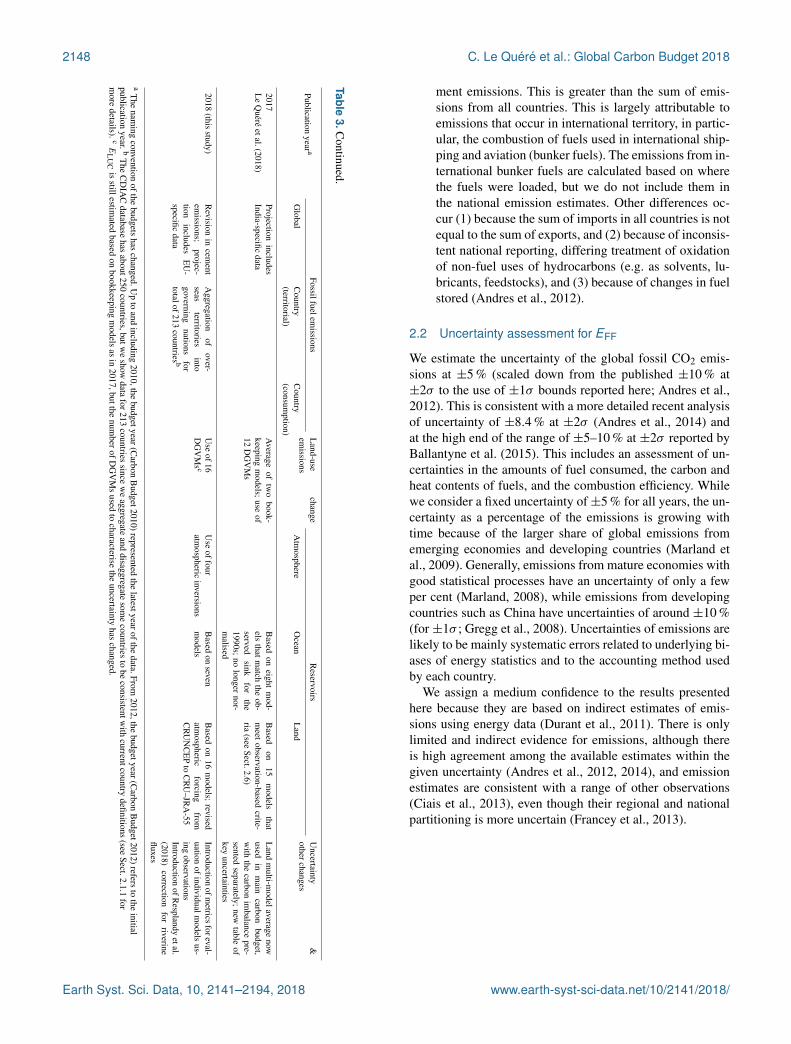
ment emissions. This is greater than the sum of emis-sions from all countries. This is largely attributable toemissions that occur in international territory, in partic-ular, the combustion of fuels used in international ship-ping and aviation (bunker fuels). The emissions from in-ternational bunker fuels are calculated based on wherethe fuels were loaded, but we do not include them inthe national emission estimates. Other differences oc-cur (1) because the sum of imports in all countries is notequal to the sum of exports, and (2) because of inconsis-tent national reporting, differing treatment of oxidationof non-fuel uses of hydrocarbons (e.g. as solvents, lu-bricants, feedstocks), and (3) because of changes in fuelstored (Andres et al., 2012).
2.2 Uncertainty assessment for EFF
We estimate the uncertainty of the global fossil CO2 emis-sions at ±5 % (scaled down from the published ±10 % at±2σ to the use of ±1σ bounds reported here; Andres et al.,2012). This is consistent with a more detailed recent analysisof uncertainty of ±8.4 % at ±2σ (Andres et al., 2014) andat the high end of the range of ±5–10 % at ±2σ reported byBallantyne et al. (2015). This includes an assessment of un-certainties in the amounts of fuel consumed, the carbon andheat contents of fuels, and the combustion efficiency. Whilewe consider a fixed uncertainty of±5 % for all years, the un-certainty as a percentage of the emissions is growing withtime because of the larger share of global emissions fromemerging economies and developing countries (Marland etal., 2009). Generally, emissions from mature economies withgood statistical processes have an uncertainty of only a fewper cent (Marland, 2008), while emissions from developingcountries such as China have uncertainties of around ±10 %(for ±1σ ; Gregg et al., 2008). Uncertainties of emissions arelikely to be mainly systematic errors related to underlying bi-ases of energy statistics and to the accounting method usedby each country.
We assign a medium confidence to the results presentedhere because they are based on indirect estimates of emis-sions using energy data (Durant et al., 2011). There is onlylimited and indirect evidence for emissions, although thereis high agreement among the available estimates within thegiven uncertainty (Andres et al., 2012, 2014), and emissionestimates are consistent with a range of other observations(Ciais et al., 2013), even though their regional and nationalpartitioning is more uncertain (Francey et al., 2013).
Earth Syst. Sci. Data, 10, 2141–2194, 2018 www.earth-syst-sci-data.net/10/2141/2018/

C. Le Quéré et al.: Global Carbon Budget 2018 2149
2.2.1 Emissions embodied in goods and services
CDIAC, UNFCCC, and BP national emission statistics “in-clude greenhouse gas emissions and removals taking placewithin national territory and offshore areas over which thecountry has jurisdiction” (Rypdal et al., 2006) and are calledterritorial emission inventories. Consumption-based emis-sion inventories allocate emissions to products that are con-sumed within a country and are conceptually calculated asthe territorial emissions minus the “embodied” territorialemissions to produce exported products plus the emissionsin other countries to produce imported products (consump-tion = territorial − exports + imports). Consumption-basedemission attribution results (e.g. Davis and Caldeira, 2010)provide additional information to territorial-based emissionsthat can be used to understand emission drivers (Hertwichand Peters, 2009) and quantify emission transfers by thetrade of products between countries (Peters et al., 2011b).The consumption-based emissions have the same global to-tal but reflect the trade-driven movement of emissions acrossthe Earth’s surface in response to human activities.
We estimate consumption-based emissions from 1990 to2016 by enumerating the global supply chain using a globalmodel of the economic relationships between economic sec-tors within and among every country (Andrew and Peters,2013; Peters et al., 2011a). Our analysis is based on the eco-nomic and trade data from the Global Trade and AnalysisProject (GTAP; Narayanan et al., 2015), and we make de-tailed estimates for the years 1997 (GTAP version 5), 2001(GTAP6), and 2004, 2007, and 2011 (GTAP9.2), covering 57sectors and 141 countries and regions. The detailed resultsare then extended into an annual time series from 1990 to thelatest year of the gross domestic product (GDP) data (2016in this budget), using GDP data by expenditure in the currentexchange rate of US dollars (USD; from the UN NationalAccounts Main Aggregrates Database; UN, 2017a) and timeseries of trade data from GTAP (based on the methodology inPeters et al., 2011b). We estimate the sector-level CO2 emis-sions using the GTAP data and methodology, include flaringand cement emissions from CDIAC, and then scale the na-tional totals (excluding bunker fuels) to match the emissionestimates from the carbon budget. We do not provide a sep-arate uncertainty estimate for the consumption-based emis-sions, but based on model comparisons and sensitivity anal-ysis, they are unlikely to be significantly different than forthe territorial emission estimates (Peters et al., 2012a).
2.2.2 Growth rate in emissions
We report the annual growth rate in emissions for adjacentyears (in per cent per year) by calculating the difference be-tween the two years and then normalising to the emissionsin the first year: (EFF(t0+1)−EFF(t0))/EFF(t0)× 100% ×100/(1 year). ×100/(1 year). We apply a leap-year adjust-ment when relevant to ensure valid interpretations of annual
growth rates. This affects the growth rate by about 0.3 % yr−1
(1/365) and causes growth rates to go up approximately0.3 % if the first year is a leap year and down 0.3 % if thesecond year is a leap year.
The relative growth rate of EFF over time periods ofgreater than 1 year can be rewritten using its logarithm equiv-alent as follows:
1EFF
dEFF
dt=
d(lnEFF)dt
. (2)
Here we calculate relative growth rates in emissions formulti-year periods (e.g. a decade) by fitting a linear trend toln(EFF) in Eq. (2), reported in per cent per year.
2.2.3 Emission projections
To gain insight into emission trends for the current year(2018), we provide an assessment of global fossil CO2 emis-sions, EFF, by combining individual assessments of emis-sions for China, the US, the EU, and India (the four coun-tries/regions with the largest emissions), and the rest of theworld.
Our 2018 estimate for China uses (1) the sum of domes-tic production (NBS, 2018b) and net imports (General Ad-ministration of Customs of the People’s Republic of China,2018) for coal, oil and natural gas, and production of cement(NBS, 2018b) from preliminary statistics for January throughSeptember of 2018 and (2) historical relationships betweenJanuary–September statistics for both production and im-ports and full-year statistics for consumption using final datafor 2000–2016 (NBS, 2015, 2017) and preliminary data for2017 (NBS, 2018a). See also Liu et al. (2018) and Jacksonet al. (2018) for details. The uncertainty is based on the vari-ance of the difference between the January–September andfull-year data from historical data, as well as typical variancein the preliminary full-year data used for 2017 and typicalchanges in the energy content of coal for the period of 2013–2016 (NBS, 2017, 2015). We note that developments for thefinal 3 months this year may be atypical due to the ongoingtrade disputes between China and the US, and this additionaluncertainty has not been quantified. Results and uncertaintiesare discussed further in Sect. 3.4.1.
For the US, we use the forecast of the U.S. Energy In-formation Administration (EIA) for emissions from fossilfuels (EIA, 2018). This is based on an energy forecastingmodel which is updated monthly (last update to October)and takes into account heating-degree days, household ex-penditures by fuel type, energy markets, policies, and othereffects. We combine this with our estimate of emissions fromcement production using the monthly US cement data fromthe U.S. Geological Survey (USGS) for January–August, as-suming changes in cement production over the first part ofthe year apply throughout the year. While the EIA’s forecastsfor current full-year emissions have on average been reviseddownwards, only 10 such forecasts are available, so we con-
www.earth-syst-sci-data.net/10/2141/2018/ Earth Syst. Sci. Data, 10, 2141–2194, 2018

2150 C. Le Quéré et al.: Global Carbon Budget 2018
servatively use the full range of adjustments following revi-sion and additionally assume symmetrical uncertainty to give±2.5 % around the central forecast.
For India, we use (1) monthly coal production and salesdata from the Ministry of Mines (2018), Coal India Lim-ited (CIL, 2018), and Singareni Collieries Company Limited(SCCL, 2018), combined with import data from the Min-istry of Commerce and Industry (MCI, 2018) and powerstation stocks data from the Central Electricity Authority(CEA, 2018); (2) monthly oil production and consumptiondata from the Ministry of Petroleum and Natural Gas (PPAC,2018a); (3) monthly natural gas production and import datafrom the Ministry of Petroleum and Natural Gas (PPAC,2018b); and (4) monthly cement production data from theOffice of the Economic Advisor (OEA, 2018). All data wereavailable for January to September or October. We use Holt–Winters exponential smoothing with multiplicative seasonal-ity (Chatfield, 1978) on each of these four emission series toproject to the end of the current year. This iterative methodproduces estimates of both trend and seasonality at the end ofthe observation period that are a function of all prior obser-vations, weighted most strongly to more recent data, whilemaintaining some smoothing effect. The main source of un-certainty in the projection of India’s emissions is the assump-tion of continued trends and typical seasonality.
For the EU, we use (1) monthly coal supply data fromEurostat for the first 6–9 months of the year (Eurostat,2018) cross-checked with more recent data on coal-generatedelectricity from ENTSO-E for January through October(ENTSO-E, 2018); (2) monthly oil and gas demand data forJanuary through August from the Joint Organisations DataInitiative (JODI, 2018); and (3) cement production assumedto be stable. For oil and gas emissions we apply the Holt–Winters method separately to each country and energy car-rier to project to the end of the current year, while for coal– which is much less strongly seasonal because of strongweather variations – we assume the remaining months of theyear are the same as the previous year in each country.
For the rest of the world, we use the close relation-ship between the growth in GDP and the growth in emis-sions (Raupach et al., 2007) to project emissions for thecurrent year. This is based on a simplified Kaya identity,whereby EFF (GtC yr−1) is decomposed by the product ofGDP (USD yr−1) and the fossil fuel carbon intensity of theeconomy (IFF; GtC USD−1) as follows:
EFF = GDP × IFF. (3)
Taking a time derivative of Eq. (3) and rearranging gives
1EFF
dEFF
dt=
1GDP
dGDPdt+
1IFF
dIFF
dt, (4)
where the left-hand term is the relative growth rate of EFF,and the right-hand terms are the relative growth rates of GDPand IFF, respectively, which can simply be added linearly togive the overall growth rate.
The growth rates are reported in per cent by multiplyingeach term by 100. As preliminary estimates of annual changein GDP are made well before the end of a calendar year, mak-ing assumptions on the growth rate of IFF allows us to makeprojections of the annual change in CO2 emissions well be-fore the end of a calendar year. The IFF is based on GDPin constant PPP (purchasing power parity) from the Inter-national Energy Agency (IEA) up until 2016 (IEA/OECD,2017) and extended using the International Monetary Fund(IMF) growth rates for 2016 and 2017 (IMF, 2018). Interan-nual variability in IFF is the largest source of uncertainty inthe GDP-based emission projections. We thus use the stan-dard deviation of the annual IFF for the period of 2007–2017as a measure of uncertainty, reflecting a ±1σ as in the restof the carbon budget. This is ±1.0 % yr−1 for the rest of theworld (global emissions minus China, the US, the EU, andIndia).
The 2018 projection for the world is made of the sum ofthe projections for China, the US, the EU, India, and the restof the world. The uncertainty is added in quadrature amongthe five regions. The uncertainty here reflects the best of ourexpert opinion.
2.3 CO2 emissions from land use, land-use change,and forestry (ELUC)
The net CO2 flux from land use, land-use change, andforestry (ELUC, called land-use change emissions in the restof the text) include CO2 fluxes from deforestation, afforesta-tion, logging and forest degradation (including harvest ac-tivity), shifting cultivation (cycle of cutting forest for agri-culture, then abandoning), and regrowth of forests followingwood harvest or abandonment of agriculture. Only some landmanagement activities are included in our land-use changeemission estimates (Table A1 in the Appendix). Some ofthese activities lead to emissions of CO2 to the atmosphere,while others lead to CO2 sinks. ELUC is the net sum ofemissions and removals due to all anthropogenic activitiesconsidered. Our annual estimate for 1959–2017 is providedas the average of results from two bookkeeping models(Sect. 2.3.1): the estimate published by Houghton and Nas-sikas (2017; hereafter H&N2017) extended here to 2017 andan estimate using the BLUE model (Bookkeeping of LandUse Emissions; Hansis et al., 2015). In addition, we use re-sults from dynamic global vegetation models (DGVMs; seeSect. 2.3.3 and Table 4) to help quantify the uncertainty inELUC and thus better characterise our understanding. Thethree methods are described below, and differences are dis-cussed in Sect. 3.2.
2.3.1 Bookkeeping models
Land-use change CO2 emissions and uptake fluxes are cal-culated by two bookkeeping models. Both are based onthe original bookkeeping approach of Houghton (2003) that
Earth Syst. Sci. Data, 10, 2141–2194, 2018 www.earth-syst-sci-data.net/10/2141/2018/

C. Le Quéré et al.: Global Carbon Budget 2018 2151
Table 4. References for the process models, pCO2-based ocean flux products, and atmospheric inversions included in Figs. 6–8. All modelsand products are updated with new data to the end of the year 2017, and the atmospheric forcing for the DGVMs has been updated asdescribed in Sect. 2.3.2.
Model/data name Reference Change from Le Quéré et al. (2018)
Bookkeeping models for land-use change emissions
BLUE Hansis et al. (2015) LUH2 rangelands were treated differently, using the static LUH2 informa-tion on forest–non-forest grid cells to determine clearing for rangelands. Ad-ditionally effects on degradation of primary to secondary lands due to range-lands on natural (uncleared) vegetation were added to BLUE.
H&N2017 Houghton and Nassikas (2017) No change.
Dynamic global vegetation modelsa
CABLE-POP Haverd et al. (2018) Simple crop harvest and grazing implemented. Small adjustments to photo-synthesis parameters to compensate for the effect of new climate forcing onGPP.
CLASS–CTEM Melton and Arora (2016) 20 soil layers used. Soil depth is prescribed following Pelletier et al. (2016).CLM5.0 Oleson et al. (2013) No change.DLEM Tian et al. (2015) Using observed irrigation data instead of a potential irrigation map.ISAM Meiyappan et al. (2015) Crop harvest and N fertiliser application as described in Song et al. (2016).JSBACH Mauritsen et al. (2018) New version of JSBACH (JSBACH 3.2), as used for CMIP6 simulations.
Changes include a new fire algorithm, as well as new processes (land nitro-gen cycle, carbon storage of wood products). Furthermore, LUH2 rangelandswere treated differently, using the static LUH2 information on forest–non-forest grid cells to determine clearing for rangelands.
JULES Clark et al. (2011) No change.LPJ-GUESS Smith et al. (2014)b No change.LPJ Poulter et al. (2011)c Uses monthly litter update (previously annual), three product pools for de-
forestation flux, shifting cultivation, wood harvest, and inclusion of borealneedleleaf deciduous plant functional type.
LPX-Bern Lienert and Joos (2018) Minor refinement of parameterization. Changed from 1◦×1◦ to 0.5◦×0.5◦
resolution. Nitrogen deposition and fertilisation from NMIP.OCN Zaehle and Friend (2010) No change (uses r294).ORCHIDEE-Trunk Krinner et al. (2005)d Updated soil water stress and albedo scheme; overall C-cycle optimisation
(gross fluxes).ORCHIDEE-CNP Goll et al. (2017) First time contribution (ORCHIDEE with nitrogen and phosphorus dynam-
ics).SDGVM Walker et al. (2017) No change.SURFEXv8 Joetzjer et al. (2015) Not applicable (not used in 2017).VISIT Kato et al. (2013) Updated spin-up protocol.
Global ocean biogeochemistry models
CCSM-BEC Doney et al. (2009) No change.MICOM-HAMOCC (NorESM-OC) Schwinger et al. (2016) No drift correction.MITgcm-REcoM2 Hauck et al. (2016) No change.MPIOM-HAMOCC Mauritsen et al. (2018) Change of atmospheric forcing; CMIP6 model version including modifica-
tions and bug fixes in HAMOCC and MPIOM.NEMO-PISCES (CNRM) Berthet et al. (2018) New model version with update to NEMOv3.6 and improved gas exchange.NEMO-PISCES (IPSL) Aumont and Bopp (2006) No change.NEMO-PlankTOM5 Buitenhuis et al. (2010)e No change.
pCO2-based flux ocean products
Landschützer Landschützer et al. (2016) No change.Jena CarboScope Rödenbeck et al. (2014) No change.
Atmospheric inversions
CAMS Chevallier et al. (2005) No change.CarbonTracker Europe (CTE) van der Laan-Luijkx et al. (2017) Minor changes in the inversion set-up.Jena CarboScope Rödenbeck et al. (2003) No change.MIROC Saeki and Patra (2017) Not applicable (not used in 2017).
a The forcing for all DGVMs has been updated from CRUNCEP to CRU–JRA. b To account for the differences between the derivation of shortwave radiation (SWRAD) from CRU cloudiness andSWRAD from CRU–JRA-55, the photosynthesis scaling parameter αa was modified (−15 %) to yield similar results. c Compared to the published version, LPJ wood harvest efficiency was decreasedso that 50 % of biomass was removed off-site compared to 85 % used in the 2012 budget. Residue management of managed grasslands increased so that 100 % of harvested grass enters the litter pool.d Compared to the published version, new hydrology and snow scheme; revised parameter values for photosynthetic capacity for all ecosystem (following assimilation of FLUXNET data), updatedparameters values for stem allocation, maintenance respiration, and biomass export for tropical forests (based on literature), and CO2 down-regulation process added to photosynthesis. Version usedfor CMIP6. e No nutrient restoring below the mixed-layer depth.
www.earth-syst-sci-data.net/10/2141/2018/ Earth Syst. Sci. Data, 10, 2141–2194, 2018

2152 C. Le Quéré et al.: Global Carbon Budget 2018
keeps track of the carbon stored in vegetation and soils be-fore and after a land-use change (transitions between variousnatural vegetation types, croplands, and pastures). Literature-based response curves describe decay of vegetation and soilcarbon, including transfer to product pools of different life-times, as well as carbon uptake due to regrowth. In addition,the bookkeeping models represent long-term degradation ofprimary forest as lowered standing vegetation and soil carbonstocks in secondary forests and also include forest manage-ment practices such as wood harvests.
The bookkeeping models do not include land ecosystems’transient response to changes in climate, atmospheric CO2,and other environmental factors, and the carbon densities arebased on contemporary data reflecting environmental condi-tions at (and up to) that time. Since carbon densities remainfixed over time in bookkeeping models, the additional sinkcapacity that ecosystems provide in response to CO2 fertili-sation and some other environmental changes is not capturedby these models (Pongratz et al., 2014; see Sect. 2.8.4).
The H&N2017 and BLUE models differ in (1) computa-tional units (country level vs. spatially explicit treatment ofland-use change), (2) processes represented (see Table A1),and (3) carbon densities assigned to vegetation and soil ofeach vegetation type. A notable change of H&N2017 overthe original approach by Houghton et al. (2003) used in ear-lier budget estimates is that no shifting cultivation or otherback-and-forth transitions below the country level are in-cluded. Only a decline in forest area in a country as indi-cated by the Forest Resource Assessment of the FAO thatexceeds the expansion of agricultural area as indicated bythe FAO is assumed to represent a concurrent expansionand abandonment of cropland. In contrast, the BLUE modelincludes sub-grid-scale transitions at the grid level amongall vegetation types as indicated by the harmonised land-use change data (LUH2) data set (https://doi.org/10.22033/ESGF/input4MIPs.1127; Hurtt et al., 2011, 2018). Further-more, H&N2017 assume conversion of natural grasslands topasture, while BLUE allocates pasture proportionally on allnatural vegetation that exists in a grid cell. This is one rea-son for generally higher emissions in BLUE. H&N2017 addcarbon emissions from peat burning based on the Global FireEmission Database (GFED4s; van der Werf et al., 2017) andpeat drainage based on estimates by Hooijer et al. (2010) tothe output of their bookkeeping model for the countries of In-donesia and Malaysia. Peat burning and emissions from theorganic layers of drained peat soils, which are not capturedby bookkeeping methods directly, need to be included to rep-resent the substantially larger emissions and interannual vari-ability due to synergies of land use and climate variability inSoutheast Asia, in particular during El Niño events. Similarlyto H&N2017, peat burning and drainage-related emissionsare also added to the BLUE estimate.
The two bookkeeping estimates used in this study also dif-fer with respect to the land-use change data used to drivethe models. H&N2017 base their estimates directly on the
Forest Resource Assessment of the FAO, which providesstatistics on forest area change and management at inter-vals of 5 years currently updated until 2015 (FAO, 2015).The data are based on country reporting to the FAO andmay include remote-sensing information in more recent as-sessments. Changes in land use other than forests are basedon annual national changes in cropland and pasture areasreported by the FAO (FAOSTAT, 2015). BLUE uses theharmonised land-use change data LUH2 (https://doi.org/10.22033/ESGF/input4MIPs.1127, Hurtt et al., 2011, 2018),which describe land-use change, also based on the FAO data,but downscaled at a quarter-degree spatial resolution, consid-ering sub-grid-scale transitions among primary forest, sec-ondary forest, cropland, pasture, and rangeland. The LUH2data provide a new distinction between rangelands and pas-ture. To constrain the models’ interpretation on whetherrangeland implies the original natural vegetation to be trans-formed to grassland or not (e.g. browsing on shrubland), anew forest mask was provided with LUH2; forest is assumedto be transformed, while all other natural vegetation remains.This is implemented in BLUE.
The estimate of H&N2017 was extended here by 2 years(to 2017) by adding the anomaly of total tropical emissions(peat drainage from Hooijer et al. (2010), peat burning, andtropical deforestation and degradation fires (from GFED4s)over the previous decade (2006–2015) to the decadal averageof the bookkeeping result.
2.3.2 Dynamic global vegetation models (DGVMs)
Land-use change CO2 emissions have also been estimatedusing an ensemble of 16 DGVM simulations. The DGVMsaccount for deforestation and regrowth, the most importantcomponents of ELUC, but they do not represent all processesresulting directly from human activities on land (Table A1).All DGVMs represent processes of vegetation growth andmortality, as well as decomposition of dead organic matterassociated with natural cycles, and include the vegetationand soil carbon response to increasing atmospheric CO2 lev-els and to climate variability and change. Some models ex-plicitly simulate the coupling of carbon and nitrogen cyclesand account for atmospheric N deposition (Table A1). TheDGVMs are independent from the other budget terms exceptfor their use of atmospheric CO2 concentration to calculatethe fertilisation effect of CO2 on plant photosynthesis.
The DGVMs used the HYDE land-use change data set(Klein Goldewijk et al., 2017a, b), which provides annualhalf-degree fractional data on cropland and pasture. Thesedata are based on annual FAO statistics of change in agricul-tural land area available until 2012. The FAOSTAT land usedatabase is updated annually, currently covering the periodof 1961–2016 (but used here until 2015 because of the tim-ing of data availability). HYDE-applied annual changes inFAO data to the year 2012 from the previous release are usedto derive new 2013–2015 data. After the year 2015 HYDE
Earth Syst. Sci. Data, 10, 2141–2194, 2018 www.earth-syst-sci-data.net/10/2141/2018/

C. Le Quéré et al.: Global Carbon Budget 2018 2153
extrapolates cropland, pasture, and urban land use data untilthe year 2018. Some models also use an update of the morecomprehensive harmonised land-use data set (Hurtt et al.,2011), which further includes fractional data on primary andsecondary forest vegetation, as well as all underlying transi-tions between land-use states (Hurtt et al., 2018; Table A1).This new data set is of quarter-degree fractional areas of landuse states and all transitions between those states, includ-ing a new wood harvest reconstruction, new representationof shifting cultivation, crop rotations, and management in-formation including irrigation and fertiliser application. Theland-use states now include five different crop types in ad-dition to the pasture–rangeland split discussed before. Woodharvest patterns are constrained with Landsat tree cover lossdata.
DGVMs implement land-use change differently (e.g.an increased cropland fraction in a grid cell can be atthe expense of either grassland or shrubs, or forest, thelatter resulting in deforestation; land cover fractions ofthe non-agricultural land differ among models). Similarly,model-specific assumptions are applied to convert deforestedbiomass or deforested area and other forest product poolsinto carbon, and different choices are made regarding the al-location of rangelands as natural vegetation or pastures.
The DGVM model runs were forced by either the mergedmonthly CRU and 6-hourly JRA-55 data set or by themonthly CRU data set, both providing observation-basedtemperature, precipitation, and incoming surface radiation ona 0.5◦× 0.5◦ grid and updated to 2017 (Harris et al., 2014).The combination of CRU monthly data with 6-hourly forc-ing is updated this year from NCEP to JRA-55 (Kobayashi etal., 2015), adapting the methodology used in previous years(Viovy, 2016) to the specifics of the JRA-55 data. The forc-ing data also include global atmospheric CO2, which changesover time (Dlugokencky and Tans, 2018) and gridded time-dependent N deposition (as used in some models; Table A1).
Two sets of simulations were performed with the DGVMs.Both applied historical changes in climate, atmospheric CO2concentration, and N deposition. The two sets of simula-tions differ, however, with respect to land use: one set ap-plies historical changes in land use, the other a time-invariantpre-industrial land cover distribution and pre-industrial woodharvest rates. By difference of the two simulations, the dy-namic evolution of vegetation biomass and soil carbon poolsin response to land use change can be quantified in eachmodel (ELUC). We only retain model outputs with positiveELUC, i.e. a positive flux to the atmosphere, during the 1990s(Table A1). Using the difference between these two DGVMsimulations to diagnose ELUC means the DGVMs accountfor the loss of additional sink capacity (around 0.3 GtC yr−1;see Sect. 2.8.4), while the bookkeeping models do not.
2.3.3 Uncertainty assessment for ELUC
Differences between the bookkeeping models and DGVMmodels originate from three main sources: the differentmethodologies, the underlying land use/land cover data set,and the different processes represented (Table A1). We exam-ine the results from the DGVM models and from the book-keeping method and use the resulting variations as a way tocharacterise the uncertainty in ELUC.
The ELUC estimate from the DGVMs multi-model meanis consistent with the average of the emissions from thebookkeeping models (Table 5). However there are large dif-ferences among individual DGVMs (standard deviation ataround 0.6–0.7 GtC yr−1; Table 5), between the two book-keeping models (average of 0.7 GtC yr−1), and between thecurrent estimate of H&N2017 and its previous model ver-sion (Houghton et al., 2012). The uncertainty in ELUC of±0.7 GtC yr−1 reflects our best value judgment that there isat least a 68 % chance (±1σ ) that the true land-use changeemission lies within the given range, for the range of pro-cesses considered here. Prior to the year 1959, the uncer-tainty in ELUC was taken from the standard deviation ofthe DGVMs. We assign low confidence to the annual esti-mates of ELUC because of the inconsistencies among esti-mates and of the difficulties to quantify some of the processesin DGVMs.
2.3.4 Emission projections
We project emissions for both H&N2017 and BLUE for2018 using the same approach as for the extrapolation ofH&N2017 for 2016–2017. Peat burning as well as tropicaldeforestation and degradation are estimated using active firedata (MCD14ML; Giglio et al., 2016), which scales almostlinearly with GFED (van der Werf et al., 2017) and thus al-lows for tracking fire emissions in deforestation and tropicalpeat zones in near-real time. During most years, emissionsduring January–October cover most of the fire season in theAmazon and Southeast Asia, where a large part of the globaldeforestation takes place.
2.4 Growth rate in atmospheric CO2 concentration(GATM)
2.4.1 Global growth rate in atmospheric CO2concentration
The rate of growth of the atmospheric CO2 concentra-tion is provided by the US National Oceanic and Atmo-spheric Administration Earth System Research Laboratory(NOAA/ESRL, 2018; Dlugokencky and Tans, 2018), whichis updated from Ballantyne et al. (2012). For the 1959–1979period, the global growth rate is based on measurements ofatmospheric CO2 concentration averaged from the MaunaLoa and South Pole stations, as observed by the CO2 Pro-gram at the Scripps Institution of Oceanography (Keeling et
www.earth-syst-sci-data.net/10/2141/2018/ Earth Syst. Sci. Data, 10, 2141–2194, 2018

2154 C. Le Quéré et al.: Global Carbon Budget 2018
Table 5. Comparison of results from the bookkeeping method and budget residuals with results from the DGVMs and inverse estimates fordifferent periods, the last decade, and the last year available. All values are in GtC yr−1. The DGVM uncertainties represent ±1σ of thedecadal or annual (for 2017 only) estimates from the individual DGVMs: for the inverse models the range of available results is given.
Mean (GtC yr−1) ±1σ
1960–1969 1970–1979 1980–1989 1990–1999 2000–2009 2008–2017 2017
Land-use change emissions (ELUC)
Bookkeeping methods 1.5± 0.7 1.2± 0.7 1.2± 0.7 1.4± 0.7 1.3± 0.7 1.5± 0.7 1.4± 0.7DGVMs 1.5± 0.7 1.4± 0.7 1.5± 0.7 1.3± 0.6 1.4± 0.6 1.9± 0.6 2.0± 0.7
Terrestrial sink (SLAND)
Residual sink from global budget(EFF+ELUC−GATM− SOCEAN)
1.8± 0.9 1.8± 0.9 1.5± 0.9 2.6± 0.9 2.9± 0.9 3.5± 1.0 4.1± 1.0
DGVMs 1.2± 0.5 2.1± 0.4 1.8± 0.6 2.4± 0.5 2.7± 0.7 3.2± 0.7 3.8± 0.8
Total land fluxes (SLAND−ELUC)
Budget constraint(EFF−GATM− SOCEAN)
0.3± 0.5 0.6± 0.6 0.4± 0.6 1.2± 0.6 1.6± 0.6 2.1± 0.7 2.7± 0.7
DGVMs −0.3± 0.6 0.7± 0.5 0.3± 0.6 1.1± 0.5 1.3± 0.5 1.3± 0.5 1.8± 0.5Inversions* –/–/– –/–/– −0.2–0.1 0.5–1.1 0.8–1.5 1.4–2.4 1.2–3.1
* Estimates are corrected for the pre-industrial influence of river fluxes and adjusted to common EFF (Sect. 2.8.2). Two inversions are available for the 1980s and 1990s.Two additional inversions are available from 2001 and used from the decade of the 2000s (Table A3).
al., 1976). For the 1980–2017 time period, the global growthrate is based on the average of multiple stations selected fromthe marine boundary layer sites with well-mixed backgroundair (Ballantyne et al., 2012), after fitting each station with asmoothed curve as a function of time and averaging by lati-tude band (Masarie and Tans, 1995). The annual growth rateis estimated by Dlugokencky and Tans (2018) from the atmo-spheric CO2 concentration by taking the average of the mostrecent December–January months corrected for the averageseasonal cycle and subtracting this same average 1 year ear-lier. The growth rate in units of ppm yr−1 is converted to unitsof GtC yr−1 by multiplying by a factor of 2.124 GtC per ppm(Ballantyne et al., 2012).
The uncertainty around the atmospheric growth rate is dueto four main factors. The first factor is the long-term repro-ducibility of reference gas standards (around 0.03 ppm for1σ from the 1980s). The second factor is that small unex-plained systematic analytical errors that may have a durationof several months to 2 years come and go. They have beensimulated by randomising both the duration and the mag-nitude (determined from the existing evidence) in a MonteCarlo procedure. The third factor is the network composi-tion of the marine boundary layer with some sites comingor going, gaps in the time series at each site, etc. (Dlu-gokencky and Tans, 2018). The latter uncertainty was esti-mated by NOAA/ESRL with a Monte Carlo method by con-structing 100 “alternative” networks (NOAA/ESRL, 2018;Masarie and Tans, 1995). The second and third uncertain-ties, summed in quadrature, add up to 0.085 ppm on aver-age (Dlugokencky and Tans, 2018). Fourth, the uncertaintyassociated with using the average CO2 concentration from
a surface network to approximate the true atmospheric av-erage CO2 concentration (mass weighted, in three dimen-sions) as needed to assess the total atmospheric CO2 bur-den. In reality, CO2 variations measured at the stations willnot exactly track changes in total atmospheric burden, withoffsets in magnitude and phasing due to vertical and hori-zontal mixing. This effect must be very small on decadal andlonger timescales, when the atmosphere can be consideredwell mixed. Preliminary estimates suggest this effect wouldincrease the annual uncertainty, but a full analysis is notyet available. We therefore maintain an uncertainty aroundthe annual growth rate based on the multiple stations’ dataset ranges between 0.11 and 0.72 GtC yr−1, with a mean of0.61 GtC yr−1 for 1959–1979 and 0.18 GtC yr−1 for 1980–2017, when a larger set of stations were available as providedby Dlugokencky and Tans (2018), but recognise further ex-ploration of this uncertainty is required. At this time, we es-timate the uncertainty of the decadal averaged growth rateafter 1980 at 0.02 GtC yr−1 based on the calibration and theannual growth rate uncertainty, but stretched over a 10-yearinterval. For years prior to 1980, we estimate the decadal av-eraged uncertainty to be 0.07 GtC yr−1 based on a factor pro-portional to the annual uncertainty prior to and after 1980(0.61/0.18× 0.02 GtC yr−1).
We assign a high confidence to the annual estimates ofGATM because they are based on direct measurements frommultiple and consistent instruments and stations distributedaround the world (Ballantyne et al., 2012).
In order to estimate the total carbon accumulated in theatmosphere since 1750 or 1870, we use an atmosphericCO2 concentration of 277± 3 ppm or 288± 3 ppm, respec-
Earth Syst. Sci. Data, 10, 2141–2194, 2018 www.earth-syst-sci-data.net/10/2141/2018/

C. Le Quéré et al.: Global Carbon Budget 2018 2155
tively, based on a cubic spline fit to ice core data (Joosand Spahni, 2008). The uncertainty of ±3 ppm (converted to±1σ ) is taken directly from the IPCC’s assessment (Ciais etal., 2013). Typical uncertainties in the growth rate in atmo-spheric CO2 concentration from ice core data are equivalentto±0.1–0.15 GtC yr−1 as evaluated from the Law Dome data(Etheridge et al., 1996) for individual 20-year intervals overthe period from 1870 to 1960 (Bruno and Joos, 1997).
2.4.2 Atmospheric growth rate projection
We provide an assessment of GATM for 2018 based on theobserved increase in atmospheric CO2 concentration at theMauna Loa station for January to October and a mean growthrate over the past 5 years for the months November to De-cember. Growth at Mauna Loa is closely correlated with theglobal growth (r = 0.95) and is used here as a proxy forglobal growth, but the regression is not 1 to 1. We also ad-just the projected global growth rate to take this into account.The assessment method used this year differs from the fore-cast method used in Le Quéré et al. (2018) based on therelationship between annual CO2 growth rate and sea sur-face temperatures (SSTs) in the Niño3.4 region of Betts etal. (2016). A change was introduced because although theobserved growth rate for 2017 of 2.2 ppm was within the pro-jection range of 2.5± 0.5 ppm of last year ( Le Quéré et al.,2018), the forecast values for 2018 for January to Octoberare too high by approximately 0.4 ppm above observed val-ues on average. The reasons for the difference are being in-vestigated. The use of observed growth at Mauna Loa Obser-vatory, Hawaii, for the first half of the year is thought to bemore robust because of its high correlation with the globalgrowth rate. Furthermore, additional analysis suggests thatthe first half of the year shows more interannual variabilitythan the second half of the year, so that the exact projectionmethod applied to November–December has only a small im-pact (< 0.1 ppm) on the projection of the full year. Uncer-tainty is estimated from past variability using the standarddeviation of the last 5 years’ monthly growth rates.
2.5 Ocean CO2 sink
Estimates of the global ocean CO2 sink SOCEAN arefrom an ensemble of global ocean biogeochemistry models(GOBMs) that meet observational constraints over the 1990s(see below). We use observation-based estimates of SOCEANto provide a qualitative assessment of confidence in the re-ported results and to estimate the cumulative accumulationof SOCEAN over the pre-industrial period.
2.5.1 Observation-based estimates
We use the observational constraints assessed by IPCC of amean ocean CO2 sink of 2.2± 0.4 GtC yr−1 for the 1990s(Denman et al., 2007) to verify that the GOBMs provide a
realistic assessment of SOCEAN. This is based on indirect ob-servations with seven different methodologies and their un-certainties, using the methods that are deemed most reliablefor the assessment of this quantity (Denman et al., 2007). TheIPCC confirmed this assessment in 2013 (Ciais et al., 2013).The observational-based estimates use the ocean–land CO2sink partitioning from observed atmospheric O2/N2 concen-tration trends (Manning and Keeling, 2006; updated in Keel-ing and Manning 2014), an oceanic inversion method con-strained by ocean biogeochemistry data (Mikaloff Fletcheret al., 2006), and a method based on a penetration timescalefor chlorofluorocarbons (McNeil et al., 2003). The IPCC esti-mate of 2.2 GtC yr−1 for the 1990s is consistent with a rangeof methods (Wanninkhof et al., 2013).
We also use two estimates of the ocean CO2 sink and itsvariability based on interpolations of measurements of sur-face ocean fugacity of CO2 (pCO2 corrected for the non-ideal behaviour of the gas; Pfeil et al., 2013). We refer tothese as pCO2-based flux estimates. The measurements arefrom the Surface Ocean CO2 Atlas version 6, which is an up-date of version 3 (Bakker et al., 2016) and contains quality-controlled data until 2017 (see data attribution Table A4).The SOCAT v6 data were mapped using a data-driven di-agnostic method (Rödenbeck et al., 2013) and a combinedself-organising map and feed-forward neural network (Land-schützer et al., 2014). The global pCO2-based flux estimateswere adjusted to remove the pre-industrial ocean source ofCO2 to the atmosphere of 0.78 GtC yr−1 from river inputto the ocean (Resplandy et al., 2018), per our definition ofSOCEAN. Several other ocean sink products based on obser-vations are also available but they continue to show largeunresolved discrepancies with observed variability. Here weused the two pCO2-based flux products that had the best fitto observations for their representation of tropical and globalvariability (Rödenbeck et al., 2015).
We further use results from two diagnostic ocean modelsof Khatiwala et al. (2013) and DeVries (2014) to estimatethe anthropogenic carbon accumulated in the ocean prior to1959. The two approaches assume constant ocean circula-tion and biological fluxes, with SOCEAN estimated as a re-sponse in the change in atmospheric CO2 concentration cali-brated to observations. The uncertainty in cumulative uptakeof ±20 GtC (converted to ±1σ ) is taken directly from theIPCC’s review of the literature (Rhein et al., 2013), or about±30 % for the annual values (Khatiwala et al., 2009).
2.5.2 Global ocean biogeochemistry models (GOBMs)
The ocean CO2 sink for 1959–2017 is estimated using sevenGOBMs (Table A2). The GOBMs represent the physical,chemical, and biological processes that influence the sur-face ocean concentration of CO2 and thus the air–sea CO2flux. The GOBMs are forced by meteorological reanalysisand atmospheric CO2 concentration data available for the en-tire time period. They mostly differ in the source of the at-
www.earth-syst-sci-data.net/10/2141/2018/ Earth Syst. Sci. Data, 10, 2141–2194, 2018

2156 C. Le Quéré et al.: Global Carbon Budget 2018
mospheric forcing data (meteorological reanalysis), spin-upstrategies, and their horizontal and vertical resolutions (Ta-ble A2). GOBMs do not include the effects of anthropogenicchanges in nutrient supply, which could lead to an increase inthe ocean sink of up to about 0.3 GtC yr−1 over the industrialperiod (Duce et al., 2008). They also do not include the per-turbation associated with changes in riverine organic carbon(see Sect. 2.8.3).
2.5.3 GOBM evaluation and uncertainty assessment forSOCEAN
The mean ocean CO2 sink for all GOBMs falls within 90 %confidence of the observed range, or 1.6 to 2.8 GtC yr−1 forthe 1990s. Here we have adjusted the confidence interval tothe IPCC confidence interval of 90 % to avoid rejecting mod-els that may be outliers but are still plausible.
The GOBMs and flux products have been further evaluatedusing fCO2 from the SOCAT v6 database. We focused thisinitial evaluation on the interannual mismatch metric pro-posed by Rödenbeck et al. (2015) for the comparison of fluxproducts. The metric provides a measure of the mismatch be-tween observations and models or flux products on the x axisas well as a measure of the amplitude of the interannual vari-ability on the y axis. A smaller number on the x axis in-dicates a better fit with observations. The amplitude of theinterannual variability in SOCEAN (y axis) is calculated as thetemporal standard deviation of the CO2 flux time series.
The calculation for the x axis is carried out as follows:(1) the mismatch between the observed and the modelledfCO2 is calculated for the period 1985 to 2017 (except forthe IPSL model, which uses 1985 to 2015 due to data avail-ability), but only for grid points for which actual observa-tions exist. (2) The interannual variability in this mismatchis calculated as the temporal standard deviation of the mis-match. (3) To put numbers into perspective, the interannualvariability in the mismatch is reported relative to the interan-nual variability in the mismatch between a benchmark fCO2field and the observations. The benchmark fCO2 field is de-signed to have no interannual variability, i.e. it is calculatedas the mean seasonal cycle at each grid point over the fullperiod plus the deseasonalised atmospheric fCO2 increaseover time. By definition, the interannual variability in themisfit between benchmark and observations is large as thebenchmark field does not contain any interannual variabil-ity from the ocean. A smaller relative interannual variabilitymismatch indicates a better fit between observed and mod-elled fCO2. This metric is chosen because it is the mostdirect measure of the year-to-year variability in SOCEAN inocean biogeochemistry models. We apply the metric glob-ally and by latitude bands. Results are shown in Fig. B1 anddiscussed in Sect. 3.1.3.
The uncertainty around the mean ocean sink of anthro-pogenic CO2 was quantified by Denman et al. (2007) forthe 1990s (see Sect. 2.5.1). To quantify the uncertainty
around annual values, we examine the standard deviationof the GOBM ensemble, which averages between 0.2 and0.3 GtC yr−1 during 1959–2017. We estimate that the uncer-tainty in the annual ocean CO2 sink is about ±0.5 GtC yr−1
from the combined uncertainty of the mean flux based onobservations of ±0.4 GtC yr−1 and the standard deviationacross GOBMs of up to ±0.3 GtC yr−1, reflecting the un-certainty in both the mean sink from observations during the1990s (Denman et al., 2007; Sect. 2.5.1) and the interannualvariability as assessed by GOBMs.
We examine the consistency between the variability inthe model-based and the pCO2-based flux products to as-sess confidence in SOCEAN. The interannual variability inthe ocean fluxes (quantified as the standard deviation) ofthe two pCO2-based flux products for 1985–2017 (wherethey overlap) is ±0.36 GtC yr−1 (Rödenbeck et al., 2014)and ±0.38 GtC yr−1 (Landschützer et al., 2015), comparedto ±0.29 GtC yr−1 for the GOBM ensemble. The standarddeviation includes a component of trend and decadal vari-ability in addition to interannual variability, and their rela-tive influence differs across estimates. Individual estimates(both GOBM and flux products) generally produce a higherocean CO2 sink during strong El Niño events. The annualpCO2-based flux products correlate with the ocean CO2 sinkestimated here with a correlation of r = 0.75 (0.59 to 0.79for individual GOBMs) and r = 0.80 (0.71 to 0.81) for thepCO2-based flux products of Rödenbeck et al. (2014) andLandschützer et al. (2015), respectively (simple linear regres-sion), with their mutual correlation at 0.73. The agreementbetween models and the flux products reflects some consis-tency in their representation of underlying variability sincethere is little overlap in their methodology or use of obser-vations. The use of annual data for the correlation may re-duce the strength of the relationship because the dominantsource of variability associated with El Niño events is lessthan 1 year. We assess a medium confidence level to the an-nual ocean CO2 sink and its uncertainty because it is basedon multiple lines of evidence, and the results are consistent inthat the interannual variability in the GOBMs and data-basedestimates are all generally small compared to the variabilityin the growth rate of atmospheric CO2 concentration.
2.6 Terrestrial CO2 sink
2.6.1 DGVM simulations
The terrestrial land sink (SLAND) is thought to be due to thecombined effects of fertilisation by rising atmospheric CO2and N deposition on plant growth, as well as the effects ofclimate change such as the lengthening of the growing sea-son in northern temperate and boreal areas. SLAND does notinclude land sinks directly resulting from land use and land-use change (e.g. regrowth of vegetation) as these are part ofthe land use flux (ELUC), although system boundaries make
Earth Syst. Sci. Data, 10, 2141–2194, 2018 www.earth-syst-sci-data.net/10/2141/2018/

C. Le Quéré et al.: Global Carbon Budget 2018 2157
it difficult to exactly attribute CO2 fluxes on land betweenSLAND and ELUC (Erb et al., 2013).SLAND is estimated from the multi-model mean of the
DGVMs (Table 4). As described in Sect. 2.3.2, DGVM sim-ulations include all climate variability and CO2 effects overland, with some DGVMs also including the effect of N de-position. The DGVMs do not include the perturbation associ-ated with changes in river organic carbon, which is discussedin Sect. 2.8.
2.6.2 DGVM evaluation and uncertainty assessment forSLAND
We apply three criteria for minimum DGVM realism byincluding only those DGVMs with (1) steady state afterspin-up; (2) net land fluxes (SLAND–ELUC) that are theatmosphere-to-land carbon flux over the 1990s ranging be-tween −0.3 and 2.3 GtC yr−1, within 90 % confidence ofconstraints by global atmospheric and oceanic observations(Keeling and Manning, 2014; Wanninkhof et al., 2013); and(3) global ELUC that is a carbon source to the atmosphereover the 1990s. All 16 DGVMs meet the three criteria.
In addition, the DGVM results are now also evaluatedusing the International Land Model Benchmarking System(ILAMB; Collier et al., 2018). This evaluation is providedhere to document, encourage, and support model improve-ments through time. ILAMB variables cover key processesthat are relevant for the quantification of SLAND and result-ing aggregated outcomes. The selected variables are vegeta-tion biomass, gross primary productivity, leaf area index, netecosystem exchange, ecosystem respiration, evapotranspira-tion, and runoff (see Fig. B2 for the results and for the list ofobserved databases). Results are shown in Fig. B2 and dis-cussed in Sect. 3.1.3.
For the uncertainty, we use the standard deviation of theannual CO2 sink across the DGVMs, which averages to±0.8 GtC yr−1 for the period from 1959 to 2017. We attacha medium confidence level to the annual land CO2 sink andits uncertainty because the estimates from the residual bud-get and averaged DGVMs match well within their respectiveuncertainties (Table 5).
2.7 The atmospheric perspective
The worldwide network of atmospheric measurements canbe used with atmospheric inversion methods to constrain thelocation of the combined total surface CO2 fluxes from allsources, including fossil and land-use change emissions andland and ocean CO2 fluxes. The inversions assume EFF to bewell known, and they solve for the spatial and temporal dis-tribution of land and ocean fluxes from the residual gradientsof CO2 among stations that are not explained by fossil fuelemissions.
Four atmospheric inversions (Table A3) used atmosphericCO2 data until the end of 2017 (including preliminary val-
ues in some cases) to infer the spatio-temporal distributionof the CO2 flux exchanged between the atmosphere and theland or oceans. We focus here on the largest and most consis-tent sources of information, namely the total land and oceanCO2 fluxes and their partitioning among the mid- to high-latitude region of the Northern Hemisphere (30–90◦ N), thetropics (30◦ S–30◦ N), and the mid- to high-latitude regionof the Southern Hemisphere (30–90◦ S). We also break downthose estimates for the land and ocean regions separately, tofurther scrutinise the constraints from atmospheric observa-tions. We use these estimates to comment on the consistencyacross various data streams and process-based estimates.
2.7.1 Atmospheric inversions
The four inversion systems used in this release are Carbon-Tracker Europe (CTE; van der Laan-Luijkx et al., 2017),Jena CarboScope (Rödenbeck, 2005), the Copernicus Atmo-sphere Monitoring Service (CAMS; Chevallier et al., 2005),and MIROC (Patra et al., 2018). See Table A3 for versionnumbers. The inversions are based on the same Bayesian in-version principles that interpret the same, for the most part,observed time series (or subsets thereof) but use differentmethodologies (Table A3). These differences mainly concernthe selection of atmospheric CO2 data, the used prior fluxes,spatial breakdown (i.e. grid size), assumed correlation struc-tures, and mathematical approach. The details of these ap-proaches are documented extensively in the references pro-vided above. Each system uses a different transport model,which was demonstrated to be a driving factor behind differ-ences in atmospheric-based flux estimates, and specificallytheir distribution across latitudinal bands (e.g. Gaubert et al.,2018).
The inversions use atmospheric CO2 observations fromvarious flask and in situ networks, as detailed in Table A3.They prescribe global EFF, which is scaled to the presentstudy for CAMS and CTE, while slightly lower EFF valuesbased on alternative emission compilations were used in Car-boScope and MIROC. Since this is known to result directlyin lower total CO2 uptake in atmospheric inversions (Gaubertet al., 2018; Peylin et al., 2013), we adjusted the land sinkof each inversion estimate (where most of the emissions oc-cur) by its fossil fuel difference to the CAMS model. Thesedifferences amount to as much as 0.7 GtC for certain years(CarboScope inversion region NH) and are thus an importantconsideration in an inverse flux comparison.
The land–ocean CO2 fluxes from atmospheric inversionscontain anthropogenic perturbation and natural pre-industrialCO2 fluxes. Natural pre-industrial fluxes are land CO2 sinkscorresponding to carbon transported to the ocean by rivers.These land CO2 sinks are compensated for over the globe byocean CO2 sources corresponding to the outgassing of river-ine carbon inputs to the ocean. We apply the distribution ofland CO2 fluxes in three latitude bands using estimates fromResplandy et al. (2018), which are constrained by ocean heat
www.earth-syst-sci-data.net/10/2141/2018/ Earth Syst. Sci. Data, 10, 2141–2194, 2018

2158 C. Le Quéré et al.: Global Carbon Budget 2018
transport to a total sink of 0.78 GtC yr−1. The latitude distri-bution of river-induced ocean CO2 sources is derived froma simulation of the IPSL GOBM using the river flux con-strained by heat transport of Resplandy et al. (2018) as aninput. We adjusted the land–ocean fluxes per latitude bandbased on these results.
The atmospheric inversions are now evaluated using ver-tical profiles of atmospheric CO2 concentrations (Fig. B3).More than 50 aircraft programmes over the globe, either reg-ular or occasional, have been used in order to draw a pic-ture of the model performance but the space–time data cov-erage is irregular, denser around 2009 or in the 0–45◦ N lat-itude band. The four models are compared to independentCO2 measurements made onboard aircraft over many placesof the world between 1 and 7 km above sea level, between2008 and 2016. Results are shown in Fig. B3 and discussedin Sect. 3.1.3.
2.8 Processes not included in the global carbon budget
The contribution of anthropogenic CO and CH4 to the globalcarbon budget has been partly neglected in Eq. (1) and is de-scribed in Sect. 2.8.1. The contributions of other carbonatesto CO2 emissions are described in Sect. 2.8.2. The contribu-tion of anthropogenic changes in river fluxes is conceptuallyincluded in Eq. (1) in SOCEAN and in SLAND, but it is not rep-resented in the process models used to quantify these fluxes.This effect is discussed in Sect. 2.8.3. Similarly, the loss ofadditional sink capacity from reduced forest cover is miss-ing in the combination of approaches used here to estimateboth land fluxes (ELUC and SLAND) and its potential effect isdiscussed and quantified in Sect. 2.8.4.
2.8.1 Contribution of anthropogenic CO and CH4 to theglobal carbon budget
Equation (1) only partly includes the net input of CO2 to theatmosphere from the chemical oxidation of reactive carbon-containing gases from sources other than the combustion offossil fuels, such as (1) cement process emissions, since thesedo not come from combustion of fossil fuels, (2) the oxi-dation of fossil fuels, and (3) the assumption of immediateoxidation of vented methane in oil production. Equation (1)omits however any other anthropogenic carbon-containinggases that are eventually oxidised in the atmosphere, suchas anthropogenic emissions of CO and CH4. An attempt ismade in this section to estimate their magnitude and iden-tify the sources of uncertainty. Anthropogenic CO emissionsare from incomplete fossil fuel and biofuel burning and de-forestation fires. The main anthropogenic emissions of fossilCH4 that matter for the global carbon budget are the fugitiveemissions of coal, oil, and gas upstream from sectors (seebelow). These emissions of CO and CH4 contribute a net ad-dition of fossil carbon to the atmosphere.
In our estimate of EFF we assumed (Sect. 2.1.1) that allthe fuel burned is emitted as CO2; thus CO anthropogenicemissions associated with incomplete combustion and theiratmospheric oxidation into CO2 within a few months are al-ready counted implicitly in EFF and should not be countedtwice (same for ELUC and anthropogenic CO emissions bydeforestation fires). Anthropogenic emissions of fossil CH4are not included in EFF because these fugitive emissions arenot included in the fuel inventories. Yet they contribute to theannual CO2 growth rate after CH4 is oxidised into CO2. An-thropogenic emissions of fossil CH4 represent 15 % of totalCH4 emissions (Kirschke et al., 2013), that is 0.061 GtC yr−1
for the past decade. Assuming steady state, these emissionsare all converted to CO2 by OH oxidation and thus explain0.06 GtC yr−1 of the global CO2 growth rate in the pastdecade, or 0.07–0.1 GtC yr−1 using the higher CH4 emis-sions reported recently (Schwietzke et al., 2016).
Other anthropogenic changes in the sources of CO andCH4 from wildfires, vegetation biomass, wetlands, rumi-nants, or permafrost changes are similarly assumed to havea small effect on the CO2 growth rate. The CH4 emissionsand sinks are published and analysed separately in the GlobalMethane Budget publication that follows an approach similarto that presented here (Saunois et al., 2016).
2.8.2 Contribution of other carbonates to CO2emissions
The contribution of fossil carbonates other than cement pro-duction is not systematically included in estimates of EFF,except at the national level at which they are accounted forin the UNFCCC national inventories. The missing processesinclude CO2 emissions associated with the calcination oflime and limestone outside cement production and the reab-sorption of CO2 by the rocks and concrete from carbonationthrough their lifetime (Xi et al., 2016). Carbonates are usedin various industries, including in iron and steel manufactureand in agriculture. They are found naturally in some coals.Carbonation from the cement life cycle, including demoli-tion and crushing, was estimated by one study to be around0.25 GtC yr−1 for the year 2013 (Xi et al., 2016). Carbona-tion emissions from the cement life cycle would offset cal-cination emissions from lime and limestone production. Thebalance of these two processes is not clear.
2.8.3 Anthropogenic carbon fluxes in the land-to-oceanaquatic continuum
The approach used to determine the global carbon budgetrefers to the mean, variations, and trends in the perturbationof CO2 in the atmosphere, referenced to the pre-industrialera. Carbon is continuously displaced from the land to theocean through the land–ocean aquatic continuum (LOAC)comprising freshwaters, estuaries, and coastal areas (Baueret al., 2013; Regnier et al., 2013). A significant fraction of
Earth Syst. Sci. Data, 10, 2141–2194, 2018 www.earth-syst-sci-data.net/10/2141/2018/

C. Le Quéré et al.: Global Carbon Budget 2018 2159
Figure 2. Schematic representation of the overall perturbation of the global carbon cycle caused by anthropogenic activities, averagedglobally for the decade 2008–2017. See legends for the corresponding arrows and units. The uncertainty in the atmospheric CO2 growthrate is very small (±0.02 GtC yr−1) and is neglected for the figure. The anthropogenic perturbation occurs on top of an active carbon cycle,with fluxes and stocks represented in the background and taken from Ciais et al. (2013) for all numbers, with the ocean fluxes updated to90 GtC yr−1 to account for the increase in atmospheric CO2 since publication, and except for the carbon stocks at the coasts, which are froma literature review of coastal marine sediments (Price and Warren, 2016).
this lateral carbon flux is entirely “natural” and is thus asteady-state component of the pre-industrial carbon cycle.We account for this pre-industrial flux where appropriate inour study. However, changes in environmental conditions andland use change have caused an increase in the lateral trans-port of carbon into the LOAC – a perturbation that is relevantfor the global carbon budget presented here.
The results of the analysis of Regnier et al. (2013) can besummarised in two points of relevance for the anthropogenicCO2 budget. First, the anthropogenic perturbation has in-creased the organic carbon export from terrestrial ecosystemsto the hydrosphere at a rate of 1.0±0.5 GtC yr−1, mainly ow-ing to enhanced carbon export from soils. Second, this ex-ported anthropogenic carbon is partly respired through theLOAC, partly sequestered in sediments along the LOAC, andto a lesser extent transferred to the open ocean where it mayaccumulate. The increase in storage of land-derived organiccarbon in the LOAC and open ocean combined is estimatedby Regnier et al. (2013) at 0.65± 0.35 GtC yr−1. We do notattempt to incorporate the changes in LOAC in our study.
The inclusion of freshwater fluxes of anthropogenic CO2affects the estimates of, and partitioning between, SLAND andSOCEAN in Eq. (1), but does not affect the other terms. Thiseffect is not included in the GOBMs and DGVMs used in ourglobal carbon budget analysis presented here.
2.8.4 Loss of additional sink capacity
Historical land-cover change was dominated by transitionsfrom vegetation types that can provide a large sink per areaunit (typically forests) to others less efficient in removingCO2 from the atmosphere (typically croplands). The resul-tant decrease in land sink, called the “loss of sink capac-ity”, is calculated as the difference between the actual landsink under changing land cover and the counterfactual landsink under pre-industrial land cover. An efficient protocolhas yet to be designed to estimate the magnitude of the lossof additional sink capacity in DGVMs. Here, we provide aquantitative estimate of this term to be used in the discus-sion. Our estimate uses the compact Earth system modelOSCAR whose land carbon cycle component is designed to
www.earth-syst-sci-data.net/10/2141/2018/ Earth Syst. Sci. Data, 10, 2141–2194, 2018

2160 C. Le Quéré et al.: Global Carbon Budget 2018
emulate the behaviour of DGVMs (Gasser et al., 2017). Weuse OSCAR v2.2.1 (an update of v2.2 with minor changes)in a probabilistic setup identical to the one of Arneth etal. (2017) but with a Monte Carlo ensemble of 2000 simula-tions. For each, we calculate SLAND and the loss of additionalsink capacity separately. We then constrain the ensemble byweighting each member to obtain a distribution of cumula-tive SLAND over 1850–2005 close to the DGVMs used here.From this ensemble, we estimate a loss of additional sinkcapacity of 0.4± 0.3 GtC yr−1 on average over 2005–2014and 20± 15 GtC accumulated between 1870 and 2017 (us-ing a linear extrapolation of the trend to estimate the last fewyears).
3 Results
3.1 Global carbon budget mean and variability for1959–2017
The global carbon budget averaged over the last half-centuryis shown in Fig. 3. For this time period, 82 % of the totalemissions (EFF+ELUC) were caused by fossil CO2 emis-sions and 18 % by land-use change. The total emissions werepartitioned among the atmosphere (45 %), ocean (24 %), andland (30 %). All components except land-use change emis-sions have grown since 1959, with important interannualvariability in the growth rate in atmospheric CO2 concen-tration and in the land CO2 sink (Fig. 4) and some decadalvariability in all terms (Table 6). Differences with previousbudget releases are documented in Fig. B4.
3.1.1 CO2 emissions
Global fossil CO2 emissions have increased every decadefrom an average of 3.1± 0.2 GtC yr−1 in the 1960s to anaverage of 9.4± 0.5 GtC yr−1 during 2008–2017 (Table 6,Figs. 2 and 5). The growth rate in these emissions decreasedbetween the 1960s and the 1990s, from 4.5 % yr−1 in the1960s (1960–1969) to 2.8 % yr−1 in the 1970s (1970–1979),1.9 % yr−1 in the 1980s (1980–1989), and 1.0 % yr−1 in the1990s (1990–1999). After this period, the growth rate be-gan increasing again in the 2000s at an average growth rateof 3.2 % yr−1, decreasing to 1.5 % yr−1 for the last decade(2008–2017), with a 3-year period of no or low growth dur-ing 2014–2016 (Fig. 5).
In contrast, CO2 emissions from land use, land-usechange, and forestry have remained relatively constant, ataround 1.3±0.7 GtC yr−1 over the past half-century but withlarge spread across estimates (Fig. 6). These emissions arealso relatively constant in the DGVM ensemble of mod-els, except during the last decade when they increase to1.9± 0.6 GtC yr−1. However, there is no agreement on thisrecent increase between the two bookkeeping models, eachsuggesting an opposite trend (Fig. 6).
Figure 3. Combined components of the global carbon budget il-lustrated in Fig. 2 as a function of time, for fossil CO2 emissions(EFF; grey) and emissions from land-use change (ELUC; brown),as well as their partitioning among the atmosphere (GATM; blue),ocean (SOCEAN; turquoise), and land (SLAND; green). The parti-tioning is based on nearly independent estimates from observations(forGATM) and from process model ensembles constrained by data(for SOCEAN and SLAND) and does not exactly add up to the sumof the emissions, resulting in a budget imbalance, which is repre-sented by the difference between the bottom pink line (reflectingtotal emissions) and the sum of the ocean, land, and atmosphere. Alltime series are in GtC yr−1. GATM and SOCEAN prior to 1959 arebased on different methods. EFF values are primarily from Bodenet al. (2017), with uncertainty of about ±5 % (±1σ ); ELUC valuesare from two bookkeeping models (Table 2) with uncertainties ofabout ±50 %; GATM prior to 1959 is from Joos and Spahni (2008)with uncertainties equivalent to about ±0.1–0.15 GtC yr−1 andfrom Dlugokencky and Tans (2018) from 1959 with uncertaintiesof about ±0.2 GtC yr−1; SOCEAN prior to 1959 is averaged fromKhatiwala et al. (2013) and DeVries (2014) with uncertainty ofabout ±30 % and from a multi-model mean (Table 4) from 1959with uncertainties of about±0.5 GtC yr−1; SLAND is a multi-modelmean (Table 4) with uncertainties of about ±0.9 GtC yr−1. See thetext for more details of each component and their uncertainties.
3.1.2 Partitioning among the atmosphere, ocean, andland
The growth rate in atmospheric CO2 level increased from1.7±0.07 GtC yr−1 in the 1960s to 4.7±0.02 GtC yr−1 dur-ing 2008–2017 with important decadal variations (Table 6and Fig. 2). Both ocean and land CO2 sinks increasedroughly in line with the atmospheric increase, but with sig-
Earth Syst. Sci. Data, 10, 2141–2194, 2018 www.earth-syst-sci-data.net/10/2141/2018/

C. Le Quéré et al.: Global Carbon Budget 2018 2161
Figure 4. Components of the global carbon budget and their uncertainties as a function of time, presented individually for (a) fossil CO2emissions (EFF), (b) emissions from land-use change (ELUC), (c) the budget imbalance that is not accounted for by the other terms,(d) growth rate in atmospheric CO2 concentration (GATM), (e) the land CO2 sink (SLAND, positive indicates a flux from the atmosphere tothe land), and (f) the ocean CO2 sink (SOCEAN, positive indicates a flux from the atmosphere to the ocean). All time series are in GtC yr−1
with the uncertainty bounds representing ±1σ in shaded colours. Data sources are as in Fig. 3. The black dots in (a) show values for 2015–2017 that originate from a different data set to the remainder of the data (see text). The dashed line in (b) identifies the pre-satellite periodbefore the inclusion of peatland burning.
nificant decadal variability on land (Table 6), and possibly inthe ocean (Fig. 7).
The ocean CO2 sink increased from 1.0± 0.5 GtC yr−1 inthe 1960s to 2.4± 0.5 GtC yr−1 during 2008–2017, with in-terannual variations of the order of a few tenths of GtC yr−1
generally showing an increased ocean sink during large ElNiño events (i.e. 1997–1998) (Fig. 7; Rödenbeck et al.,2014). Although there is some coherence among the GOBMsand pCO2-based flux products regarding the mean, there is
poor agreement for interannual variability, and the oceanmodels underestimate decadal variability (Sect. 2.5.3 andFig. 7; DeVries et al., 2017).
The terrestrial CO2 sink increased from 1.2±0.5 GtC yr−1
in the 1960s to 3.2± 0.7 GtC yr−1 during 2008–2017, withimportant interannual variations of up to 2 GtC yr−1 gener-ally showing a decreased land sink during El Niño events(Fig. 6), responsible for the corresponding enhanced growthrate in atmospheric CO2 concentration. The larger land CO2
www.earth-syst-sci-data.net/10/2141/2018/ Earth Syst. Sci. Data, 10, 2141–2194, 2018

2162 C. Le Quéré et al.: Global Carbon Budget 2018
Table 6. Decadal mean in the five components of the anthropogenic CO2 budget for different periods and the last year available. All valuesare in GtC yr−1, and uncertainties are reported as ±1σ . The table also shows the budget imbalance (BIM), which provides a measure ofthe discrepancies among the nearly independent estimates and has an uncertainty exceeding ±1 GtC yr−1. A positive imbalance means theemissions are overestimated and/or the sinks are too small.
Mean (GtC yr−1)
1960–1969 1970–1979 1980–1989 1990–1999 2000–2009 2008–2017 2017
Total emissions (EFF+ELUC)
Fossil CO2 emissions (EFF) 3.1± 0.2 4.7± 0.2 5.4± 0.3 6.3± 0.3 7.8± 0.4 9.4± 0.5 9.9± 0.5Land-use change emissions (ELUC) 1.5± 0.7 1.2± 0.7 1.2± 0.7 1.4± 0.7 1.3± 0.7 1.5± 0.7 1.4± 0.7
Total emissions 4.7± 0.7 5.8± 0.7 6.6± 0.8 7.6± 0.8 9.0± 0.8 10.8± 0.8 11.3± 0.9
Partitioning
Growth rate in atmospheric CO2 concentra-tion (GATM)
1.7± 0.07 2.8± 0.07 3.4± 0.02 3.1± 0.02 4.0± 0.02 4.7± 0.02 4.6± 0.2
Ocean sink (SOCEAN) 1.0± 0.5 1.3± 0.5 1.7± 0.5 2.0± 0.5 2.1± 0.5 2.4± 0.5 2.5± 0.5Terrestrial sink (SLAND) 1.2± 0.5 2.1± 0.4 1.8± 0.6 2.4± 0.5 2.7± 0.7 3.2± 0.7 3.8± 0.8
Budget imbalance
BIM = EFF+ELUC−(GATM+SOCEAN+SLAND)
(0.6) (−0.3) (−0.3) (0.2) (0.2) (0.5) (0.3)
sink during 2008–2017 compared to the 1960s is reproducedby all the DGVMs in response to the combined atmosphericCO2 increase and changes in climate, and consistent withconstraints from the other budget terms (Table 5).
Estimates of total atmosphere-to-land fluxes (SLAND–ELUC) from the DGVMs are consistent with the budgetconstraints (Table 5), except during 2008–2017, when theDGVM ensemble estimates a total atmosphere-to-land fluxof 1.3± 0.5 GtC yr−1, likely below the budget constraints of2.1± 0.7 GtC yr−1 and outside the range of the inversions(Table 5). This comparison suggests that the DGVMs couldoverestimate ELUC emissions and/or underestimate the ter-restrial sink SLAND during the last decade.
3.1.3 Model evaluation
The evaluation of ocean estimates (Fig. B1) shows a relativeinterannual mismatch of 15 % and 17 % for the two pCO2-based flux products over the globe, relative to the pCO2observations from the SOCAT v6 database for the period1985–2017. A 0 % mismatch would indicate a perfect model,and a field with no interannual variability would result in a100 % mismatch. A mismatch larger than 100 % is possiblewhen the method produces a larger mismatch than the bench-mark field with no interannual variability (see Sect. 2.5.3).This mismatch by the pCO2-based flux products is improvedcompared with earlier published versions of these two fluxproducts of around 20 %–25 % for the 1992–2009 time pe-riod (Rödenbeck et al., 2015), likely because of the largerdata availability after 2009. The GOBMs show a global rela-tive interannual mismatch between 50 % and 60 %, with onemodel at 94 % and one at 193 %. The GOBM mismatch is of
the same order as the mismatch calculated in an ensemble of14 flux products but larger than the two flux products usedin this report (Fig. 5 in Rödenbeck et al., 2015). The mis-match is generally larger at high latitudes compared to thetropics, for both the flux products and the GOBMs. The twoflux products have a similar mismatch of around 10 %–15 %in the tropics, around 25 % in the north, and 30 %–55 % in thesouth. The GOBM mismatch is more spread across regions,ranging from 29 % to 178 % in the tropics, 70 % to 192 %in the north, and 108 % to 304 % in the south. The highermismatch occurs in regions with stronger climate variability,such as the northern and southern high latitudes (poleward ofthe subtropical gyres) and the equatorial Pacific. The latter isalso apparent in the model mismatch but is hidden in Fig. B1due to the averaging over 30◦ S to 30◦ N (see also Sect. 4).
The evaluation of the DGVMs (Fig. B2) shows generallyhigh skill scores across models for runoff, and to a lesser ex-tent for vegetation biomass, GPP, and ecosystem respiration(Fig. B2, left panel). The skill score was lowest for leaf areaindex and net ecosystem exchange, with the widest disparityamong models for soil carbon. Further analysis of the resultswill be provided separately, focusing on the strengths andweaknesses in the DGVM ensemble and its validity for usein the global carbon budget.
The evaluation of the atmospheric inversions (Fig. B3)shows long-term mean biases in the free troposphere betterthan 0.8 ppm in absolute values for each product. CAMS andCTE biases show some dependency on latitude (a trend of−0.0018± 0.0005 and 0.0043± 0.0004 ppm per degree forCAMS and CTE, respectively). These latitude-dependent bi-ases may reveal biases in the surface fluxes (e.g. Houwelinget al., 2015) but the link is not straightforward and will be
Earth Syst. Sci. Data, 10, 2141–2194, 2018 www.earth-syst-sci-data.net/10/2141/2018/

C. Le Quéré et al.: Global Carbon Budget 2018 2163
Figure 5. Fossil CO2 emissions for (a) the globe, including an uncertainty of ±5 % (grey shading), and the emissions extrapolated using BPenergy statistics (black dots); (b) global emissions by fuel type, including coal (salmon), oil (olive), gas (turquoise), and cement (purple), andexcluding gas flaring, which is small (0.6 % in 2013); (c) territorial (solid lines) and consumption (dashed lines) emissions for the top threecountry emitters (US – olive; China – salmon; India – purple) and for the European Union (EU; turquoise for the 28 member states of theEU as of 2012); and (d) per capita emissions for the top three country emitters, the EU (all colours as in panel c), and the world (black). In(b–c), the dots show the data that were extrapolated from BP energy statistics for 2014–2016. All time series are in GtC yr−1 except the percapita emissions (d), which are in tonnes of carbon per person per year (tC person−1 yr−1). Territorial emissions are primarily from Bodenet al. (2017) except national data for the US and EU28 (the 28 member states of the EU) for 1990–2016, which are reported by the countriesto the UNFCCC as detailed in the text; consumption-based emissions are updated from Peters et al. (2011a). See Sect. 2.1.1 for details of thecalculations and data sources.
analysed separately. The biases for MIROC and CarboScopebehave similarly together in relative values, but they are lessregular than the two other products, which hampers the in-terpretation. Lesser model performance for specific aircraftprogrammes, like for the 4-year DISCOVER-AQ campaignin the continental US (https://discover-aq.larc.nasa.gov/, lastaccess: 28 November 2018), contributes to this variability.
3.1.4 Budget imbalance
The carbon budget imbalance (BIM; Eq. 1) quantifies the mis-match between the estimated total emissions and the esti-mated changes in the atmosphere, land, and ocean reservoirs.The mean budget imbalance from 1959 to 2017 is small(0.14 GtC yr−1) and shows no trend over the full time series.The process models (GOBMs and DGVMs) have been se-lected to match observational constraints in the 1990s but nofurther constraints have been applied to their representation
of trend and variability. Therefore, the near-zero mean andtrend in the budget imbalance are indirect evidence of a co-herent community understanding of the emissions and theirpartitioning on those timescales (Fig. 4). However, the bud-get imbalance shows substantial variability on the order of±1 GtC yr−1, particularly over semi-decadal timescales, al-though most of the variability is within the uncertainty of theestimates. The positive carbon imbalance during the 1960s,early 1990s, and in the last decade suggests that either theemissions were overestimated or the sinks were underesti-mated during these periods. The reverse is true for the 1970sand around 1995–2000 (Fig. 4).
We cannot attribute the cause of the variability in the bud-get imbalance with our analysis, only to note that the budgetimbalance is unlikely to be explained by errors or biases inthe emissions alone because of its large semi-decadal vari-ability component, a variability that is untypical of emissions
www.earth-syst-sci-data.net/10/2141/2018/ Earth Syst. Sci. Data, 10, 2141–2194, 2018

2164 C. Le Quéré et al.: Global Carbon Budget 2018
Figure 6. CO2 exchanges between the atmosphere and the terres-trial biosphere as used in the global carbon budget (black with±1σuncertainty in grey shading), for (a) CO2 emissions from land-usechange (ELUC), also individually showing the two bookkeepingmodels (two brown lines) and the DGVM model results (green)and their multi-model mean (dark green). The dashed line identi-fies the pre-satellite period before the inclusion of peatland burn-ing. (b) Land CO2 sink (SLAND) with individual DGVMs (green);(c) total land CO2 fluxes (b–a) with individual DGVMs (green) andtheir multi-model mean (dark green).
Figure 7. Comparison of the anthropogenic atmosphere–oceanCO2 flux showing the budget values of SOCEAN (black; with ±1σuncertainty in grey shading), individual ocean models (blue), andthe two ocean pCO2-based flux products (dark blue; see Table 4).Both pCO2-based flux products were adjusted for the pre-industrialocean source of CO2 from river input to the ocean, which is notpresent in the ocean models, by adding a sink of 0.78 GtC yr−1 (Re-splandy et al., 2018), to make them comparable to SOCEAN. Thisadjustment does not take into account the anthropogenic contribu-tion to river fluxes (see Sect. 2.8.3).
and has not changed in the past 50 years in spite of a nearlytripling in emissions (Fig. 4). Errors in SLAND and SOCEANare more likely to be the main cause for the budget imbal-ance. For example, underestimation of SLAND by DGVMshas been reported following the eruption of Mount Pinatuboin 1991 possibly due to missing responses to changes indiffuse radiation (Mercado et al., 2009) or other yet un-known factors, and DGVMs are suspected to overestimatethe land sink in response to the wet decade of the 1970s(Sitch et al., 2008). Decadal and semi-decadal variability inthe ocean sink has been also reported recently (DeVries et al.,2017; Landschützer et al., 2015), with the pCO2-based oceanflux products suggesting a smaller-than-expected ocean CO2sink in the 1990s and a larger-than-expected sink in the2000s (Fig. 7), possibly caused by changes in ocean circula-tion (DeVries et al., 2017) not captured in coarse-resolutionGOBMs used here (Dufour et al., 2013). The absence ofinternal variability could also be at fault. Internal variabil-ity is not captured by single realisations of coarse-resolutionmodel simulations (Li and Ilyina, 2018) and is thought to belargest in regions with strong seasonal and interannual cli-mate variability, i.e. the high-latitude ocean regions (pole-ward of the subtropical gyres) and the equatorial Pacific(McKinley et al., 2016). Some of these errors could be drivenby errors in the climatic forcing data, particularly precipita-tion (for SLAND) and wind (for SOCEAN), rather than in themodels.
Earth Syst. Sci. Data, 10, 2141–2194, 2018 www.earth-syst-sci-data.net/10/2141/2018/
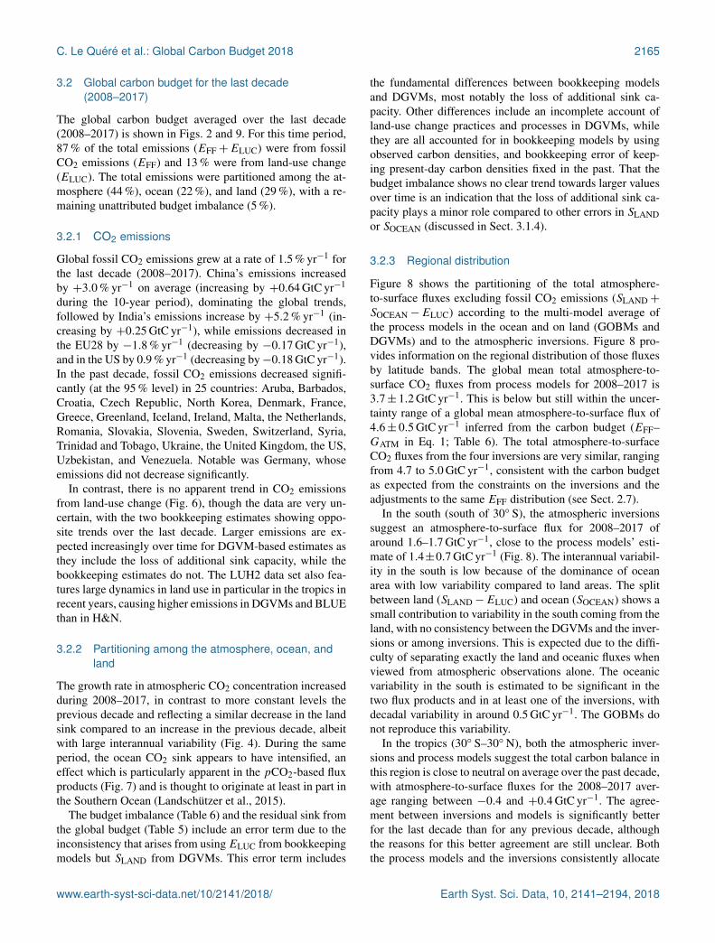
C. Le Quéré et al.: Global Carbon Budget 2018 2165
3.2 Global carbon budget for the last decade(2008–2017)
The global carbon budget averaged over the last decade(2008–2017) is shown in Figs. 2 and 9. For this time period,87 % of the total emissions (EFF+ELUC) were from fossilCO2 emissions (EFF) and 13 % were from land-use change(ELUC). The total emissions were partitioned among the at-mosphere (44 %), ocean (22 %), and land (29 %), with a re-maining unattributed budget imbalance (5 %).
3.2.1 CO2 emissions
Global fossil CO2 emissions grew at a rate of 1.5 % yr−1 forthe last decade (2008–2017). China’s emissions increasedby +3.0 % yr−1 on average (increasing by +0.64 GtC yr−1
during the 10-year period), dominating the global trends,followed by India’s emissions increase by +5.2 % yr−1 (in-creasing by +0.25 GtC yr−1), while emissions decreased inthe EU28 by −1.8 % yr−1 (decreasing by −0.17 GtC yr−1),and in the US by 0.9 % yr−1 (decreasing by−0.18 GtC yr−1).In the past decade, fossil CO2 emissions decreased signifi-cantly (at the 95 % level) in 25 countries: Aruba, Barbados,Croatia, Czech Republic, North Korea, Denmark, France,Greece, Greenland, Iceland, Ireland, Malta, the Netherlands,Romania, Slovakia, Slovenia, Sweden, Switzerland, Syria,Trinidad and Tobago, Ukraine, the United Kingdom, the US,Uzbekistan, and Venezuela. Notable was Germany, whoseemissions did not decrease significantly.
In contrast, there is no apparent trend in CO2 emissionsfrom land-use change (Fig. 6), though the data are very un-certain, with the two bookkeeping estimates showing oppo-site trends over the last decade. Larger emissions are ex-pected increasingly over time for DGVM-based estimates asthey include the loss of additional sink capacity, while thebookkeeping estimates do not. The LUH2 data set also fea-tures large dynamics in land use in particular in the tropics inrecent years, causing higher emissions in DGVMs and BLUEthan in H&N.
3.2.2 Partitioning among the atmosphere, ocean, andland
The growth rate in atmospheric CO2 concentration increasedduring 2008–2017, in contrast to more constant levels theprevious decade and reflecting a similar decrease in the landsink compared to an increase in the previous decade, albeitwith large interannual variability (Fig. 4). During the sameperiod, the ocean CO2 sink appears to have intensified, aneffect which is particularly apparent in the pCO2-based fluxproducts (Fig. 7) and is thought to originate at least in part inthe Southern Ocean (Landschützer et al., 2015).
The budget imbalance (Table 6) and the residual sink fromthe global budget (Table 5) include an error term due to theinconsistency that arises from usingELUC from bookkeepingmodels but SLAND from DGVMs. This error term includes
the fundamental differences between bookkeeping modelsand DGVMs, most notably the loss of additional sink ca-pacity. Other differences include an incomplete account ofland-use change practices and processes in DGVMs, whilethey are all accounted for in bookkeeping models by usingobserved carbon densities, and bookkeeping error of keep-ing present-day carbon densities fixed in the past. That thebudget imbalance shows no clear trend towards larger valuesover time is an indication that the loss of additional sink ca-pacity plays a minor role compared to other errors in SLANDor SOCEAN (discussed in Sect. 3.1.4).
3.2.3 Regional distribution
Figure 8 shows the partitioning of the total atmosphere-to-surface fluxes excluding fossil CO2 emissions (SLAND+
SOCEAN−ELUC) according to the multi-model average ofthe process models in the ocean and on land (GOBMs andDGVMs) and to the atmospheric inversions. Figure 8 pro-vides information on the regional distribution of those fluxesby latitude bands. The global mean total atmosphere-to-surface CO2 fluxes from process models for 2008–2017 is3.7± 1.2 GtC yr−1. This is below but still within the uncer-tainty range of a global mean atmosphere-to-surface flux of4.6± 0.5 GtC yr−1 inferred from the carbon budget (EFF–GATM in Eq. 1; Table 6). The total atmosphere-to-surfaceCO2 fluxes from the four inversions are very similar, rangingfrom 4.7 to 5.0 GtC yr−1, consistent with the carbon budgetas expected from the constraints on the inversions and theadjustments to the same EFF distribution (see Sect. 2.7).
In the south (south of 30◦ S), the atmospheric inversionssuggest an atmosphere-to-surface flux for 2008–2017 ofaround 1.6–1.7 GtC yr−1, close to the process models’ esti-mate of 1.4±0.7 GtC yr−1 (Fig. 8). The interannual variabil-ity in the south is low because of the dominance of oceanarea with low variability compared to land areas. The splitbetween land (SLAND−ELUC) and ocean (SOCEAN) shows asmall contribution to variability in the south coming from theland, with no consistency between the DGVMs and the inver-sions or among inversions. This is expected due to the diffi-culty of separating exactly the land and oceanic fluxes whenviewed from atmospheric observations alone. The oceanicvariability in the south is estimated to be significant in thetwo flux products and in at least one of the inversions, withdecadal variability in around 0.5 GtC yr−1. The GOBMs donot reproduce this variability.
In the tropics (30◦ S–30◦ N), both the atmospheric inver-sions and process models suggest the total carbon balance inthis region is close to neutral on average over the past decade,with atmosphere-to-surface fluxes for the 2008–2017 aver-age ranging between −0.4 and +0.4 GtC yr−1. The agree-ment between inversions and models is significantly betterfor the last decade than for any previous decade, althoughthe reasons for this better agreement are still unclear. Boththe process models and the inversions consistently allocate
www.earth-syst-sci-data.net/10/2141/2018/ Earth Syst. Sci. Data, 10, 2141–2194, 2018

2166 C. Le Quéré et al.: Global Carbon Budget 2018
Figure 8. CO2 fluxes between the atmosphere and the surface (SOCEAN+ SLAND−ELUC) by latitude bands for the (top) globe (secondrow), north (north of 30◦ N), (third row) tropics (30◦ S–30◦ N), and (bottom) south (south of 30◦ S) and (left) total, (middle) land only(SLAND−ELUC), and (right) ocean only. Positive values indicate a flux from the atmosphere to the land and/or ocean. Estimates from thecombination of the process models for the land and oceans are shown (black for the total, green for the land, blue for the ocean) with ±1σ ofthe model ensemble (in grey). Results from the atmospheric inversions (pink lines) and from the pCO2-based flux products (dark blue lines)are also shown.
more year-to-year variability in CO2 fluxes to the tropicscompared to the north (north of 30◦ N; Fig. 8). The splitbetween the land and ocean indicates the land is the originof most of the tropical variability, consistently among mod-els (both for the land and for the ocean) and inversions. Theoceanic variability in the tropics is similar among models andwith the two ocean flux products, reflected in their lower ob-servational mismatch (Sect. 3.1.3). While the inversions in-dicate that atmosphere-to-land CO2 fluxes are more variablethan atmosphere-to-ocean CO2 fluxes in the tropics, the cor-
respondence between the inversions and the ocean flux prod-ucts or GOBMs is much poorer.
In the north (north of 30◦ N), the inversions and pro-cess models show less agreement on the magnitude of theatmosphere-to-land flux, with the ensemble mean of the pro-cess models suggesting a total Northern Hemisphere sinkfor 2008–2017 of 2.2± 0.6 GtC yr−1, likely below the esti-mates from the inversions ranging from 2.6 to 3.6 GtC yr−1
(Fig. 8). The discrepancy in the north-tropics distributionof CO2 fluxes between the inversions and models arisesfrom the differences in mean fluxes over the northern land.
Earth Syst. Sci. Data, 10, 2141–2194, 2018 www.earth-syst-sci-data.net/10/2141/2018/

C. Le Quéré et al.: Global Carbon Budget 2018 2167
This discrepancy is also evidenced over the previous decadeand highlights not only persistent issues with the quantifi-cation of the drivers of the net land CO2 flux (Arneth etal., 2017; Huntzinger et al., 2017) but also the distributionof atmosphere-to-land fluxes between the tropics and higherlatitudes that is particularly marked in previous decades, ashighlighted previously (Stephens et al., 2007; Baccini et al.,2017; Schimel et al., 2015).
Differences between inversions may be related for exam-ple to differences in their interhemispheric transport, andother inversion settings (Table A3). Separate analysis hasshown that the influence of the chosen prior land and oceanfluxes is minor compared to other aspects of each inversion.In comparison to the previous global carbon budget publi-cation, the fossil fuel inputs were adjusted to match thoseof EFF used in this analysis (see Sect. 2.7), therefore re-moving differences due to prior fossil emissions. Differencesbetween inversions and the ensemble of process models inthe north cannot be simply explained. They could either re-flect a bias in the inversions or missing processes or biasesin the process models, such as the lack of adequate parame-terisations for forest management in the north and for forestdegradation emissions in the tropics for the DGVMs. Theestimated contribution of the north and its uncertainty fromprocess models is sensitive to both the ensemble of processmodels used and the specifics of each inversion.
Resolving the differences in the Northern Hemisphereland sink will require the consideration and inclusion oflarger volumes of semi-continuous observations from talltowers close to the surface CO2 exchange. Some of these dataare becoming available but not used in the current inversemodels, sometimes due to the short records and sometimesbecause the coarse transport models cannot adequately rep-resent these time series. Improvements in model resolutionand atmospheric transport realism together with expansionof the observational record (also in the data-sparse BorealEurasian area) will help anchor the mid-latitude fluxes percontinent. In addition, new metrics could potentially differ-entiate between the more and less realistic realisations of theNorthern Hemisphere land sink shown in Fig. 8.
3.2.4 Budget imbalance
The budget imbalance was +0.5 GtC yr−1 on average over2008–2017. Although the uncertainties are large in eachterm, the sustained imbalance over this last decade suggestsan overestimation of the emissions and/or an underestimationof the sinks. An origin in the land and/or ocean sink may bemore likely, given the large variability in the land sink and thesuspected underestimation of decadal variability in the oceansink. An underestimate of SLAND would also reconcile modelresults with inversion estimates for fluxes in the total landduring the past decade (Fig. 8; Table 5). However, we cannotexclude that the budget imbalance over the last decade couldpartly be due to an overestimation of CO2 emissions from
land-use change, given their large uncertainty, as has beensuggested elsewhere (Piao et al., 2018). More integrated useof observations in the Global Carbon Budget, either on theirown or for further constraining model results, should helpresolve some of the budget imbalance (Peters et al., 2017;Sect. 4).
3.3 Global carbon budget for the year 2017
3.3.1 CO2 emissions
Preliminary estimates of global fossil CO2 emissions basedon BP energy statistics are for emissions growing by 1.6 %between 2016 and 2017 to 9.9±0.5 GtC in 2017 (Fig. 5), dis-tributed among coal (40 %), oil (35 %), gas (20 %), cement(4 %), and gas flaring (0.7 %). Compared to the previousyear, emissions from coal increased by 1.6 %, while emis-sions from oil, gas, and cement increased by 1.7 %, 3.0 %,and 1.2 %, respectively. All growth rates presented are ad-justed for the leap year, unless stated otherwise.
The growth in emissions of 1.6 % in 2017 is within therange of the projected growth of 2.0 % (range of 0.8 to 3.0 %)published in Le Quéré et al. (2018) based on national emis-sion projections for China, the US, and India and projectionsof gross domestic product corrected for IFF trends for the restof the world. The growth in emissions in 2017 for China, theUS, and the rest of the world is also within their previouslyprojected range, while the growth in India was slightly abovethe projection (Table 7).
In 2017, the largest absolute contributions to global CO2emissions were from China (27 %), the US (15 %), the EU(28 member states; 10 %), and India (7 %) while the rest ofthe world contributed 42 %. The percentages are the frac-tion of the global emissions including bunker fuels (3.1 %).These four regions account for 59 % of global CO2 emis-sions. Growth rates for these countries from 2016 to 2017were +1.5 % (China), −0.5 % (US), +1.2 % (EU28), and+3.9 % (India), with +1.9 % for the rest of the world. Theper capita CO2 emissions in 2017 were 1.1 tC person−1 yr−1
for the globe and were 4.4 (US), 2.0 (China), 1.9 (EU28),and 0.5 (India) tC person−1 yr−1 for the four highest emittingcountries (Fig. 5).
In 2016 (the last year available), the largest absolute con-tributions to global CO2 emissions from a consumption per-spective were China (25 %), the US (16 %), the EU (12 %),and India (6 %). The difference between territorial and con-sumption emissions (the net emission transfer via interna-tional trade) has generally increased from 1990 to around2005 and remained relatively stable afterwards until the lastyear available (2016; Fig. 5).
The global CO2 emissions from land-use change are esti-mated as 1.4±0.7 GtC in 2017, close to the previous decadebut with low confidence in the annual change. This brings thetotal CO2 emissions from fossil fuels plus land-use change(EFF+ELUC) to 11.3± 0.9 GtC (41.2± 3 GtCO2).
www.earth-syst-sci-data.net/10/2141/2018/ Earth Syst. Sci. Data, 10, 2141–2194, 2018
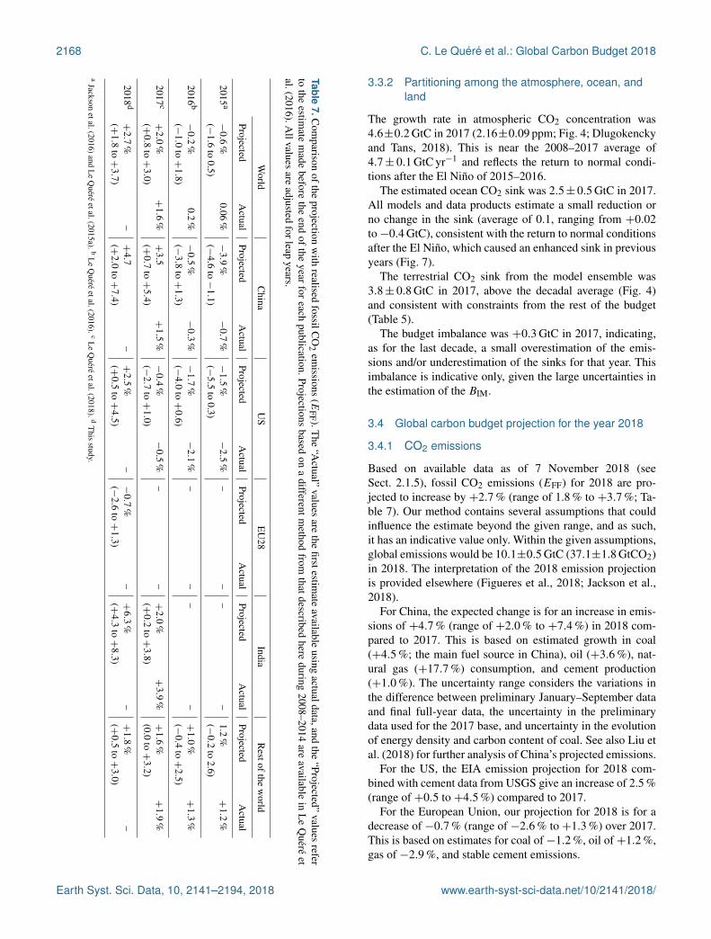
2168 C. Le Quéré et al.: Global Carbon Budget 2018
Table7.C
omparison
oftheprojection
with
realisedfossilC
O2
emissions
(EFF ).T
he“A
ctual”values
arethe
firstestimate
availableusing
actualdata,andthe
“Projected”values
referto
theestim
atem
adebefore
theend
ofthe
yearfor
eachpublication.Projections
basedon
adifferentm
ethodfrom
thatdescribedhere
during2008–2014
areavailable
inL
eQ
uéréet
al.(2016).Allvalues
areadjusted
forleapyears.
World
China
US
EU
28India
Restofthe
world
ProjectedA
ctualProjected
Actual
ProjectedA
ctualProjected
Actual
ProjectedA
ctualProjected
Actual
2015 a−
0.6
%(−
1.6
to0.5)
0.06%
−3.9
%(−
4.6
to−
1.1)
−0.7
%−
1.5
%(−
5.5
to0.3)
−2.5
%–
––
–1.2
%(−
0.2
to2.6)
+1.2
%
2016 b−
0.2
%(−
1.0
to+
1.8)
0.2%
−0.5
%(−
3.8
to+
1.3)
−0.3
%−
1.7
%(−
4.0
to+
0.6)
−2.1
%–
––
–+
1.0
%(−
0.4
to+
2.5)
+1.3
%
2017 c+
2.0
%(+
0.8
to+
3.0)
+1.6
%+
3.5
(+0.7
to+
5.4)
+1.5
%−
0.4
%(−
2.7
to+
1.0)
−0.5
%–
–+
2.0
%(+
0.2
to+
3.8)
+3.9
%+
1.6
%(0.0
to+
3.2)
+1.9
%
2018 d+
2.7
%(+
1.8
to+
3.7)
–+
4.7
(+2.0
to+
7.4)
–+
2.5
%(+
0.5
to+
4.5)
–−
0.7
%(−
2.6
to+
1.3)
–+
6.3
%(+
4.3
to+
8.3)
–+
1.8
%(+
0.5
to+
3.0)
–
aJackson
etal.(2016)andL
eQ
uéréetal.(2015a). b
Le
Quéré
etal.(2016). cL
eQ
uéréetal.(2018). d
This
study.
3.3.2 Partitioning among the atmosphere, ocean, andland
The growth rate in atmospheric CO2 concentration was4.6±0.2 GtC in 2017 (2.16±0.09 ppm; Fig. 4; Dlugokenckyand Tans, 2018). This is near the 2008–2017 average of4.7± 0.1 GtC yr−1 and reflects the return to normal condi-tions after the El Niño of 2015–2016.
The estimated ocean CO2 sink was 2.5±0.5 GtC in 2017.All models and data products estimate a small reduction orno change in the sink (average of 0.1, ranging from +0.02to−0.4 GtC), consistent with the return to normal conditionsafter the El Niño, which caused an enhanced sink in previousyears (Fig. 7).
The terrestrial CO2 sink from the model ensemble was3.8± 0.8 GtC in 2017, above the decadal average (Fig. 4)and consistent with constraints from the rest of the budget(Table 5).
The budget imbalance was +0.3 GtC in 2017, indicating,as for the last decade, a small overestimation of the emis-sions and/or underestimation of the sinks for that year. Thisimbalance is indicative only, given the large uncertainties inthe estimation of the BIM.
3.4 Global carbon budget projection for the year 2018
3.4.1 CO2 emissions
Based on available data as of 7 November 2018 (seeSect. 2.1.5), fossil CO2 emissions (EFF) for 2018 are pro-jected to increase by +2.7 % (range of 1.8 % to +3.7 %; Ta-ble 7). Our method contains several assumptions that couldinfluence the estimate beyond the given range, and as such,it has an indicative value only. Within the given assumptions,global emissions would be 10.1±0.5 GtC (37.1±1.8 GtCO2)in 2018. The interpretation of the 2018 emission projectionis provided elsewhere (Figueres et al., 2018; Jackson et al.,2018).
For China, the expected change is for an increase in emis-sions of +4.7 % (range of +2.0 % to +7.4 %) in 2018 com-pared to 2017. This is based on estimated growth in coal(+4.5 %; the main fuel source in China), oil (+3.6 %), nat-ural gas (+17.7 %) consumption, and cement production(+1.0 %). The uncertainty range considers the variations inthe difference between preliminary January–September dataand final full-year data, the uncertainty in the preliminarydata used for the 2017 base, and uncertainty in the evolutionof energy density and carbon content of coal. See also Liu etal. (2018) for further analysis of China’s projected emissions.
For the US, the EIA emission projection for 2018 com-bined with cement data from USGS give an increase of 2.5 %(range of +0.5 to +4.5 %) compared to 2017.
For the European Union, our projection for 2018 is for adecrease of −0.7 % (range of −2.6 % to +1.3 %) over 2017.This is based on estimates for coal of −1.2 %, oil of +1.2 %,gas of −2.9 %, and stable cement emissions.
Earth Syst. Sci. Data, 10, 2141–2194, 2018 www.earth-syst-sci-data.net/10/2141/2018/

C. Le Quéré et al.: Global Carbon Budget 2018 2169
Figure 9. Cumulative changes during 1870–2017 and mean fluxes during 2008–2017 for the anthropogenic perturbation as defined in thelegend.
For India, our projection for 2018 is for an increase of+6.3 % (range of 4.3 % to +8.3 %) over 2017. This is basedon separate projections for coal (+7.1 %), oil (+2.9 %), gas(+6.0 %), and cement (+13.4 %).
For the rest of the world, the expected growth for 2018is +1.8 % (range of +0.5 % to +3.0 %). This is computedusing the GDP projection for the world excluding China, theUS, the EU, and India of 2.8 % made by the IMF (IMF, 2018)and a decrease in IFF of −1.0 % yr−1, which is the averagefrom 2008 to 2017. The uncertainty range is based on thestandard deviation of the interannual variability in IFF during2008–2017 of ±0.7 % yr−1 and our estimate of uncertaintyin the IMF’s GDP forecast of ±0.5 %.
Preliminary estimates of fire emissions in deforestationzones indicate that emissions from land-use change (ELUC)for 2018 were below average until October and are expectedto range between 0.1 and 0.2 lower than the 2008–2017average. We therefore expect ELUC emissions of around
1.2 GtC in 2018, for total CO2 emissions of 11.3± 0.9 GtC(41.5± 3 GtCO2).
3.4.2 Partitioning among the atmosphere, ocean, andland
The 2018 growth in atmospheric CO2 concentration (GATM)is projected to be 4.9± 0.7 GtC (2.3± 0.3 ppm) based onMLO observations until the end of October 2018, bringingthe atmospheric CO2 concentration to an expected level of407 ppm averaged over the year. Combining projected EFF,ELUC, and GATM suggests a combined land and ocean sink(SLAND+SOCEAN) of about 6.5 GtC for 2018. Although eachterm has large uncertainty, the oceanic sink SOCEAN has gen-erally low interannual variability and is likely to remain closeto its 2017 value of around 2.5 GtC, leaving a rough es-timated land sink SLAND of around 4.0 GtC. If realised, itwould be among the largest SLAND values over the historical
www.earth-syst-sci-data.net/10/2141/2018/ Earth Syst. Sci. Data, 10, 2141–2194, 2018
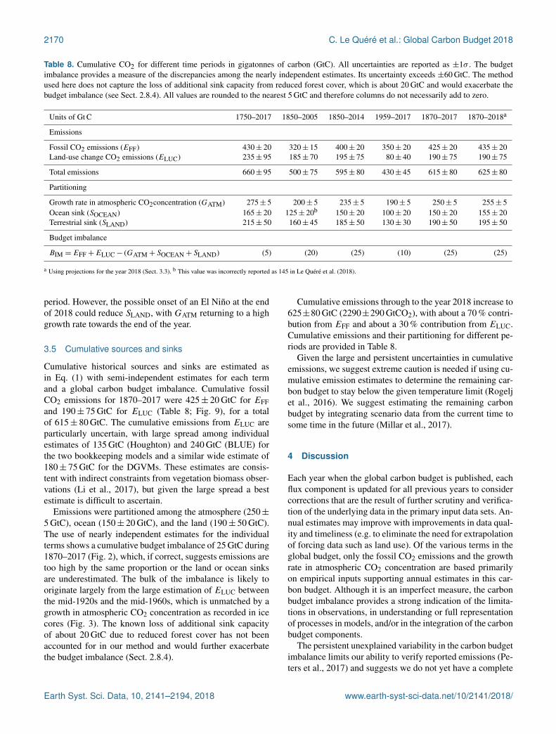
2170 C. Le Quéré et al.: Global Carbon Budget 2018
Table 8. Cumulative CO2 for different time periods in gigatonnes of carbon (GtC). All uncertainties are reported as ±1σ . The budgetimbalance provides a measure of the discrepancies among the nearly independent estimates. Its uncertainty exceeds ±60 GtC. The methodused here does not capture the loss of additional sink capacity from reduced forest cover, which is about 20 GtC and would exacerbate thebudget imbalance (see Sect. 2.8.4). All values are rounded to the nearest 5 GtC and therefore columns do not necessarily add to zero.
Units of Gt C 1750–2017 1850–2005 1850–2014 1959–2017 1870–2017 1870–2018a
Emissions
Fossil CO2 emissions (EFF) 430± 20 320± 15 400± 20 350± 20 425± 20 435± 20Land-use change CO2 emissions (ELUC) 235± 95 185± 70 195± 75 80± 40 190± 75 190± 75
Total emissions 660± 95 500± 75 595± 80 430± 45 615± 80 625± 80
Partitioning
Growth rate in atmospheric CO2concentration (GATM) 275± 5 200± 5 235± 5 190± 5 250± 5 255± 5Ocean sink (SOCEAN) 165± 20 125± 20b 150± 20 100± 20 150± 20 155± 20Terrestrial sink (SLAND) 215± 50 160± 45 185± 50 130± 30 190± 50 195± 50
Budget imbalance
BIM = EFF+ELUC− (GATM+ SOCEAN+ SLAND) (5) (20) (25) (10) (25) (25)
a Using projections for the year 2018 (Sect. 3.3). b This value was incorrectly reported as 145 in Le Quéré et al. (2018).
period. However, the possible onset of an El Niño at the endof 2018 could reduce SLAND, with GATM returning to a highgrowth rate towards the end of the year.
3.5 Cumulative sources and sinks
Cumulative historical sources and sinks are estimated asin Eq. (1) with semi-independent estimates for each termand a global carbon budget imbalance. Cumulative fossilCO2 emissions for 1870–2017 were 425± 20 GtC for EFFand 190± 75 GtC for ELUC (Table 8; Fig. 9), for a totalof 615± 80 GtC. The cumulative emissions from ELUC areparticularly uncertain, with large spread among individualestimates of 135 GtC (Houghton) and 240 GtC (BLUE) forthe two bookkeeping models and a similar wide estimate of180± 75 GtC for the DGVMs. These estimates are consis-tent with indirect constraints from vegetation biomass obser-vations (Li et al., 2017), but given the large spread a bestestimate is difficult to ascertain.
Emissions were partitioned among the atmosphere (250±5 GtC), ocean (150± 20 GtC), and the land (190± 50 GtC).The use of nearly independent estimates for the individualterms shows a cumulative budget imbalance of 25 GtC during1870–2017 (Fig. 2), which, if correct, suggests emissions aretoo high by the same proportion or the land or ocean sinksare underestimated. The bulk of the imbalance is likely tooriginate largely from the large estimation of ELUC betweenthe mid-1920s and the mid-1960s, which is unmatched by agrowth in atmospheric CO2 concentration as recorded in icecores (Fig. 3). The known loss of additional sink capacityof about 20 GtC due to reduced forest cover has not beenaccounted for in our method and would further exacerbatethe budget imbalance (Sect. 2.8.4).
Cumulative emissions through to the year 2018 increase to625±80 GtC (2290±290 GtCO2), with about a 70 % contri-bution from EFF and about a 30 % contribution from ELUC.Cumulative emissions and their partitioning for different pe-riods are provided in Table 8.
Given the large and persistent uncertainties in cumulativeemissions, we suggest extreme caution is needed if using cu-mulative emission estimates to determine the remaining car-bon budget to stay below the given temperature limit (Rogeljet al., 2016). We suggest estimating the remaining carbonbudget by integrating scenario data from the current time tosome time in the future (Millar et al., 2017).
4 Discussion
Each year when the global carbon budget is published, eachflux component is updated for all previous years to considercorrections that are the result of further scrutiny and verifica-tion of the underlying data in the primary input data sets. An-nual estimates may improve with improvements in data qual-ity and timeliness (e.g. to eliminate the need for extrapolationof forcing data such as land use). Of the various terms in theglobal budget, only the fossil CO2 emissions and the growthrate in atmospheric CO2 concentration are based primarilyon empirical inputs supporting annual estimates in this car-bon budget. Although it is an imperfect measure, the carbonbudget imbalance provides a strong indication of the limita-tions in observations, in understanding or full representationof processes in models, and/or in the integration of the carbonbudget components.
The persistent unexplained variability in the carbon budgetimbalance limits our ability to verify reported emissions (Pe-ters et al., 2017) and suggests we do not yet have a complete
Earth Syst. Sci. Data, 10, 2141–2194, 2018 www.earth-syst-sci-data.net/10/2141/2018/

C. Le Quéré et al.: Global Carbon Budget 2018 2171
Table 9. Major known sources of uncertainties in each component of the global carbon budget, defined as input data or processes that havea demonstrated effect of at least ±0.3 GtC yr−1.
Source of uncertainty Timescale (years) Location Status Evidence
Fossil CO2 emissions (EFF; Sect. 2.1)
Energy statistics annual to decadal mainly China see Sect. 2.1 Korsbakken et al. (2016)Carbon content of coal decadal mainly China see Sect. 2.1 Liu et al. (2015)
Emissions from land-use change (ELUC; Sect. 2.3)
Land cover and land-use changestatistics
continuous global; in particular tropics see Sect. 2.3 Houghton et al. (2012)
Sub-grid-scale transitions annual to decadal global see Table A1 Wilkenskjeld et al. (2014)Vegetation biomass annual to decadal global; in particular tropics see Table A1 Houghton et al. (2012)Wood and crop harvest annual to decadal global; SE Asia see Table A1 Arneth et al. (2017)Peat burninga multi-decadal trend global see Table A1 van der Werf et al. (2010)Loss of additional sink capacity multi-decadal trend global not included;
Sect. 2.8.4Gitz and Ciais (2003)
Atmospheric growth rate (GATM)→ no demonstrated uncertainties larger than ±0.3 GtC yr−1b
Ocean sink (SOCEAN)
Variability in oceanic circulationc semi-decadal to decadal global; in particular South-ern Ocean
see Sect. 2.5.2 DeVries et al. (2017)
Internal variability annual to decadal high latitudes; equatorialPacific
no ensembles/coarseresolution
McKinley et al. (2016)
Anthropogenic changes in nutrient sup-ply
multi-decadal trend global not included Duce et al. (2008)
Land sink (SLAND)
Strength of CO2 fertilisation multi-decadal trend global see Sect. 2.6 Wenzel et al. (2016)Response to variability in temperatureand rainfall
annual to decadal global; in particular tropics see Sect. 2.6 Cox et al. (2013)
Nutrient limitation and supply multi-decadal trend global see Sect. 2.6 Zaehle et al. (2011)Response to diffuse radiation annual global see Sect. 2.6 Mercado et al. (2009)
a As a result of interactions between land use and climate. b The uncertainties in GATM have been estimated as ±0.2 GtC yr−1, although the conversion of the growth rate into aglobal annual flux assuming instantaneous mixing throughout the atmosphere introduces additional errors that have not yet been quantified. c Could in part be due to uncertainties inatmospheric forcing (Swart et al., 2014).
understanding of the underlying carbon cycle processes. Re-solving most of this unexplained variability should be possi-ble through different and complementary approaches. First,as intended with our annual updates, the imbalance as an er-ror term is reduced by improvements of individual compo-nents of the global carbon budget that follow from improvingthe underlying data and statistics and by improving the mod-els through the resolution of some of the key uncertaintiesdetailed in Table 9. Second, additional clues to the origin andprocesses responsible for the current imbalance could be ob-tained through a closer scrutiny of carbon variability in lightof other Earth system data (e.g. heat balance, water balance),and the use of a wider range of biogeochemical observationsto better understand the land–ocean partitioning of the carbonimbalance (e.g. oxygen, carbon isotopes). Finally, additionalinformation could also be obtained through higher resolutionand process knowledge at the regional level and through theintroduction of inferred fluxes such as those based on satel-lite CO2 retrievals. The limit of the resolution of the car-bon budget imbalance is yet unclear but most certainly not
yet reached given the possibilities for improvements that lieahead.
The assessment of the GOBMs used for SOCEAN with fluxproducts based on observations highlights substantial dis-crepancy at mid-latitudes and high latitudes. Given the gooddata coverage of pCO2 observations in the Northern Hemi-sphere (Bakker et al., 2016), this discrepancy points to an un-derestimation of variability in the GOBMs globally, and con-sequently the variability in SOCEAN appears to be underesti-mated. The size of this underestimate (order of 0.5 GtC yr−1)could account for some of the budget imbalance, but not all.Increasing model resolution and incorporating internal vari-ability (Li and Ilyina, 2018) have been suggested as ways toincrease model variability (Sect. 3.1.4).
The assessment of the net land–atmosphere exchange de-rived from land sink and net land use change flux with atmo-spheric inversions also shows substantial discrepancy, partic-ularly for the estimate of the total land flux over the northernextra-tropics in the past decade. This discrepancy highlightsthe difficulty to quantify complex processes (CO2 fertilisa-tion, nitrogen deposition, climate change and variability, land
www.earth-syst-sci-data.net/10/2141/2018/ Earth Syst. Sci. Data, 10, 2141–2194, 2018

2172 C. Le Quéré et al.: Global Carbon Budget 2018
management, etc.) that collectively determine the net landCO2 flux. Resolving the differences in the Northern Hemi-sphere land sink will require the consideration and inclusionof larger volumes of observations (Sect. 3.2.3).
Estimates of ELUC suffer from a range of intertwinedissues, including the poor quality of historical land coverand land-use change maps, the rudimentary representationof management processes in most models, and the confu-sion in methodologies and boundary conditions used acrossmethods (e.g. Pongratz et al., 2014; Arneth et al., 2017, andSect. 2.8.4 on the loss of sink capacity). Uncertainties in cur-rent and historical carbon stocks in soils and vegetation alsoadd uncertainty in the land-use change flux estimates. Unlessa major effort to resolve these issues is made, little progress isexpected in the resolution of ELUC. This is particularly con-cerning given the growing importance of ELUC for climatemitigation strategies and the large issues in the quantificationof the cumulative emissions over the historical period thatarise from large uncertainties in ELUC.
To move towards the resolution of the carbon budget im-balance, this year we have introduced metrics for the evalu-ation of the ocean and land models and atmospheric inver-sions. These metrics expand the use of observations in theglobal carbon budget, helping (1) to support improvementsin the ocean and land carbon models that produce the sinkestimates and (2) to constrain the representation of key un-derlying processes in the models and to allocate the regionalpartitioning of the CO2 fluxes. This is an initial step towardsthe introduction of a broader range of observations that wehope will support continued improvements in the annual es-timates of the global carbon budget.
We assessed elsewhere (Peters et al., 2017) that a sus-tained decrease of −1 % in global emissions could be de-tected at the 66 % likelihood level after a decade only. Sim-ilarly, a change in behaviour of the land and/or ocean car-bon sink would take as long to detect, and much longer ifit emerges more slowly. Reducing the carbon imbalance, re-gionalising the carbon budget, and integrating multiple vari-ables are powerful ways to shorten the detection limit andensure the research community can rapidly identify growingissues of concern in the evolution of the global carbon cycleunder the current rapid and unprecedented changing environ-mental conditions.
5 Data availability
The data presented here are made available in the belief thattheir wide dissemination will lead to greater understandingand new scientific insights into how the carbon cycle works,how humans are altering it, and how we can mitigate the re-sulting human-driven climate change. The free availabilityof these data does not constitute permission for publicationof the data. For research projects, if the data are essential tothe work, or if an important result or conclusion depends on
the data, co-authorship may need to be considered. Full con-tact details and information on how to cite the data shownhere are given at the top of each page in the accompanyingdatabase and summarised in Table 2.
The accompanying database includes two Excel filesorganised in the following spreadsheets (accessible withthe free viewer https://support.microsoft.com/en-gb/help/273711/how-to-obtain-the-latest-excel-viewer, last access:28 November 2018):
File Global_Carbon_Budget_2018v1.0.xlsx (Global Car-bon Project, 2018) includes the following:
1. summary;
2. the global carbon budget (1959–2017),
3. global CO2 emissions from fossil fuels and cement pro-duction by fuel type and the per capita emissions (1959–2017),
4. CO2 emissions from land-use change from the individ-ual methods and models (1959–2017),
5. ocean CO2 sink from the individual ocean models andpCO2-based products (1959–2017),
6. terrestrial CO2 sink from the DGVMs (1959–2017),
7. additional information on the carbon balance prior to1959 (1750–2017).
File National_Carbon_Emissions_2018v1.0.xlsx (GlobalCarbon Project, 2018) includes the following:
1. summary
2. territorial country CO2 emissions from fossil CO2 emis-sions (1959–2017) from CDIAC with UNFCCC dataoverwritten where available, extended to 2017 using BPdata;
3. consumption country CO2 emissions from fossil CO2emissions and emission transfer from the interna-tional trade of goods and services (1990–2016) usingCDIAC/UNFCCC data (worksheet 3 above) as refer-ence;
4. emission transfers (consumption minus territorial emis-sions; 1990–2016);
5. country definitions;
6. details of disaggregated countries;
7. details of aggregated countries.
National emission data are also available from the GlobalCarbon Atlas (http://www.globalcarbonatlas.org/, last ac-cess: 28 November 2018).
Earth Syst. Sci. Data, 10, 2141–2194, 2018 www.earth-syst-sci-data.net/10/2141/2018/

C. Le Quéré et al.: Global Carbon Budget 2018 2173
6 Conclusions
The estimation of global CO2 emissions and sinks is a ma-jor effort by the carbon cycle research community that re-quires a careful compilation and synthesis of measurements,statistical estimates, and model results. The delivery of anannual carbon budget serves two purposes. First, there is alarge demand for up-to-date information on the state of theanthropogenic perturbation of the climate system and its un-derpinning causes. A broad stakeholder community relies onthe data sets associated with the annual carbon budget includ-ing scientists, policymakers, businesses, journalists, and non-governmental organisations engaged in adapting to and mit-igating human-driven climate change. Second, over the lastdecade we have seen unprecedented changes in the humanand biophysical environments (e.g. changes in the growthof fossil fuel emissions, Earth’s temperatures, and strengthof the carbon sinks), which call for frequent assessments ofthe state of the planet and a growing understanding of andimproved capacity to anticipate the evolution of the carboncycle in the future. Building this scientific understanding tomeet the extraordinary climate mitigation challenge requiresfrequent, robust, and transparent data sets and methods thatcan be scrutinised and replicated. This paper via living datahelps to keep track of new budget updates.
www.earth-syst-sci-data.net/10/2141/2018/ Earth Syst. Sci. Data, 10, 2141–2194, 2018
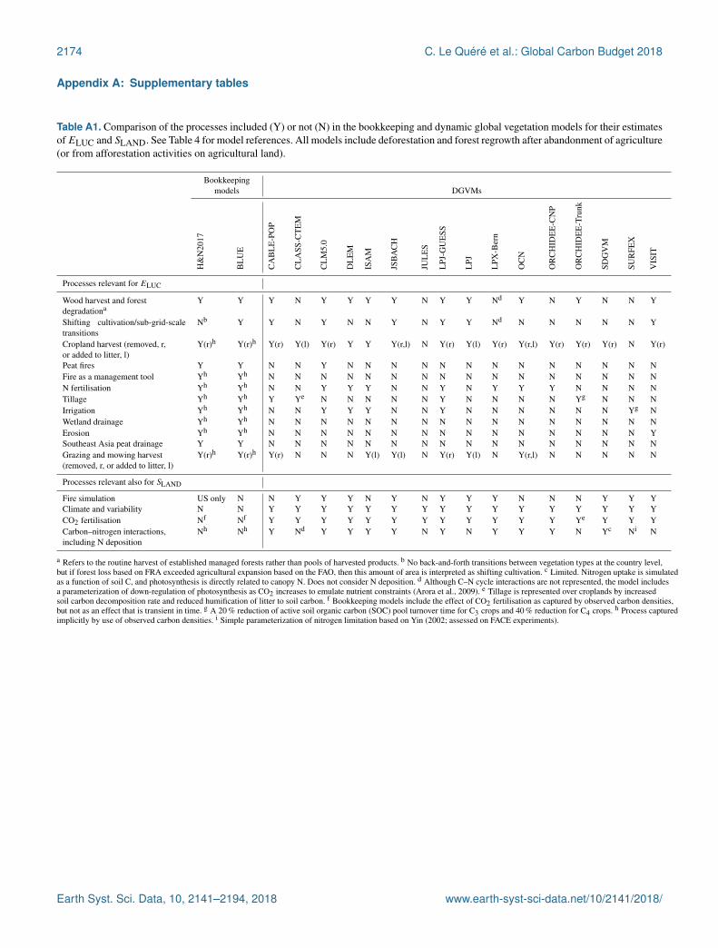
2174 C. Le Quéré et al.: Global Carbon Budget 2018
Appendix A: Supplementary tables
Table A1. Comparison of the processes included (Y) or not (N) in the bookkeeping and dynamic global vegetation models for their estimatesofELUC and SLAND. See Table 4 for model references. All models include deforestation and forest regrowth after abandonment of agriculture(or from afforestation activities on agricultural land).
Bookkeepingmodels DGVMs
H&
N20
17
BL
UE
CA
BL
E-P
OP
CL
ASS
-CT
EM
CL
M5.
0
DL
EM
ISA
M
JSB
AC
H
JUL
ES
LPJ
-GU
ESS
LPJ
LPX
-Ber
n
OC
N
OR
CH
IDE
E-C
NP
OR
CH
IDE
E-T
runk
SDG
VM
SUR
FEX
VIS
IT
Processes relevant for ELUC
Wood harvest and forestdegradationa
Y Y Y N Y Y Y Y N Y Y Nd Y N Y N N Y
Shifting cultivation/sub-grid-scaletransitions
Nb Y Y N Y N N Y N Y Y Nd N N N N N Y
Cropland harvest (removed, r,or added to litter, l)
Y(r)h Y(r)h Y(r) Y(l) Y(r) Y Y Y(r,l) N Y(r) Y(l) Y(r) Y(r,l) Y(r) Y(r) Y(r) N Y(r)
Peat fires Y Y N N Y N N N N N N N N N N N N NFire as a management tool Yh Yh N N N N N N N N N N N N N N N NN fertilisation Yh Yh N N Y Y Y N N Y N Y Y Y N N N NTillage Yh Yh Y Ye N N N N N Y N N N N Yg N N NIrrigation Yh Yh N N Y Y Y N N Y N N N N N N Yg NWetland drainage Yh Yh N N N N N N N N N N N N N N N NErosion Yh Yh N N N N N N N N N N N N N N N YSoutheast Asia peat drainage Y Y N N N N N N N N N N N N N N N NGrazing and mowing harvest(removed, r, or added to litter, l)
Y(r)h Y(r)h Y(r) N N N Y(l) Y(l) N Y(r) Y(l) N Y(r,l) N N N N N
Processes relevant also for SLAND
Fire simulation US only N N Y Y Y N Y N Y Y Y N N N Y Y YClimate and variability N N Y Y Y Y Y Y Y Y Y Y Y Y Y Y Y YCO2 fertilisation Nf Nf Y Y Y Y Y Y Y Y Y Y Y Y Ye Y Y YCarbon–nitrogen interactions,including N deposition
Nh Nh Y Nd Y Y Y Y N Y N Y Y Y N Yc Ni N
a Refers to the routine harvest of established managed forests rather than pools of harvested products. b No back-and-forth transitions between vegetation types at the country level,but if forest loss based on FRA exceeded agricultural expansion based on the FAO, then this amount of area is interpreted as shifting cultivation. c Limited. Nitrogen uptake is simulatedas a function of soil C, and photosynthesis is directly related to canopy N. Does not consider N deposition. d Although C–N cycle interactions are not represented, the model includesa parameterization of down-regulation of photosynthesis as CO2 increases to emulate nutrient constraints (Arora et al., 2009). e Tillage is represented over croplands by increasedsoil carbon decomposition rate and reduced humification of litter to soil carbon. f Bookkeeping models include the effect of CO2 fertilisation as captured by observed carbon densities,but not as an effect that is transient in time. g A 20 % reduction of active soil organic carbon (SOC) pool turnover time for C3 crops and 40 % reduction for C4 crops. h Process capturedimplicitly by use of observed carbon densities. i Simple parameterization of nitrogen limitation based on Yin (2002; assessed on FACE experiments).
Earth Syst. Sci. Data, 10, 2141–2194, 2018 www.earth-syst-sci-data.net/10/2141/2018/
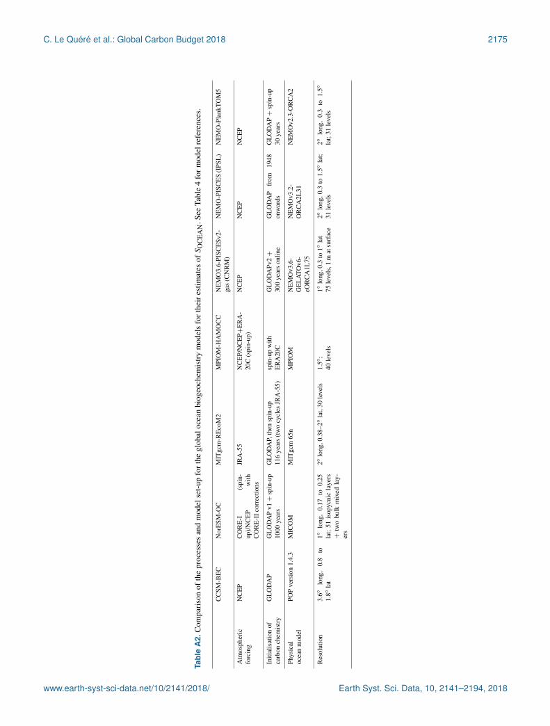
C. Le Quéré et al.: Global Carbon Budget 2018 2175
Tabl
eA
2.C
ompa
riso
nof
the
proc
esse
san
dm
odel
set-
upfo
rthe
glob
aloc
ean
biog
eoch
emis
try
mod
els
fort
heir
estim
ates
ofS
OC
EA
N.S
eeTa
ble
4fo
rmod
elre
fere
nces
.
CC
SM-B
EC
Nor
ESM
-OC
MIT
gcm
-RE
coM
2M
PIO
M-H
AM
OC
CN
EM
O3.
6-PI
SCE
Sv2-
gas
(CN
RM
)N
EM
O-P
ISC
ES
(IPS
L)
NE
MO
-Pla
nkTO
M5
Atm
osph
eric
forc
ing
NC
EP
CO
RE
-I(s
pin-
up)/
NC
EP
with
CO
RE
-IIc
orre
ctio
ns
JRA
-55
NC
EP/
NC
EP+
ER
A-
20C
(spi
n-up
)N
CE
PN
CE
PN
CE
P
Initi
alis
atio
nof
carb
onch
emis
try
GL
OD
AP
GL
OD
AP
v1+
spin
-up
1000
year
sG
LO
DA
P,th
ensp
in-u
p11
6ye
ars
(tw
ocy
cles
JRA
-55)
spin
-up
with
ER
A20
CG
LO
DA
Pv2+
300
year
son
line
GL
OD
AP
from
1948
onw
ards
GL
OD
AP+
spin
-up
30ye
ars
Phys
ical
ocea
nm
odel
POP
vers
ion
1.4.
3M
ICO
MM
ITgc
m65
nM
PIO
MN
EM
Ov3
.6-
GE
LA
TOv6
-eO
RC
A1L
75
NE
MO
v3.2
-O
RC
A2L
31N
EM
Ov2
.3-O
RC
A2
Res
olut
ion
3.6◦
long
,0.
8to
1.8◦
lat
1◦lo
ng,
0.17
to0.
25la
t;51
isop
ycni
cla
yers
+tw
obu
lkm
ixed
lay-
ers
2◦lo
ng,0
.38–
2◦la
t,30
leve
ls1.
5◦;
40le
vels
1◦lo
ng,0
.3to
1◦la
t75
leve
ls,1
mat
surf
ace
2◦lo
ng,0
.3to
1.5◦
lat;
31le
vels
2◦lo
ng,
0.3
to1.
5◦
lat;
31le
vels
www.earth-syst-sci-data.net/10/2141/2018/ Earth Syst. Sci. Data, 10, 2141–2194, 2018

2176 C. Le Quéré et al.: Global Carbon Budget 2018
Table A3. Comparison of the inversion set-up and input fields for the atmospheric inversions. Atmospheric inversions see the full CO2 fluxes,including the anthropogenic and pre-industrial fluxes. Hence they need to be adjusted for the pre-industrial flux of CO2 from the land to theocean that is part of the natural carbon cycle before they can be compared with SOCEAN and SLAND from process models. See Table 4 forreferences.
CarbonTracker Europe(CTE)
Jena CarboScope CAMS MIROC
Version number CTE2018 s85oc_v4.2 v17r1 tdi84_2018
Observations
Atmosphericobservations
Hourly resolution(well-mixed con-ditions) ObsPackGLOBALVIEWplusv3.2 & NRTv4.2a
Flasks and hourly (outliersremoved by 2σ criterion)
Daily averages of well-mixed conditions – Ob-sPack GLOBALVIEWplusv3.2a & NRT v4.2, WD-CGG, RAMCES, and ICOSATC
Flask and continuous dataat remote sites from Ob-sPack GLOBALVIEWplusv3.2 and v4.0
Prior fluxes
Biosphere and fires SiBCASA–GFED4sb No prior ORCHIDEE (climatologi-cal), GFEDv4 & GFAS
Climatological CASA with3-hourly downscaling
Ocean Ocean inversion by Ja-cobson et al. (2007)
pCO2-based ocean fluxproduct oc_v1.6 (update ofRödenbeck et al., 2014)
Landschützer et al. (2015) Takahashi et al. (2009)
Fossil fuels EDGAR+IER, scaledto CDIAC
CDIAC (extended after2013 with GCP totals)
EDGAR scaled to CDIAC EDGARv4.3.2 (2012 mapafter 2013)
Transport and optimisation
Transport model TM5 TM3 LMDZ v5A MIROC4–ACTMWeather forcing ECMWF NCEP ECMWF JRA-55Resolution (degrees) Global: 3◦× 2◦,
Europe: 1◦× 1◦,North America: 1◦×1◦
Global: 4◦× 5◦ Global: 3.75◦× 1.875◦ Global: 2.8◦× 2.8◦
Optimisation Ensemble Kalman filter Conjugate gradient(re-ortho-normalisation)c
Variational Matrix method, 84 regions
a GLOBALVIEW (2016); CarbonTracker Team (2017). b Van der Velde et al. (2014). c Ocean prior not optimised.
Earth Syst. Sci. Data, 10, 2141–2194, 2018 www.earth-syst-sci-data.net/10/2141/2018/
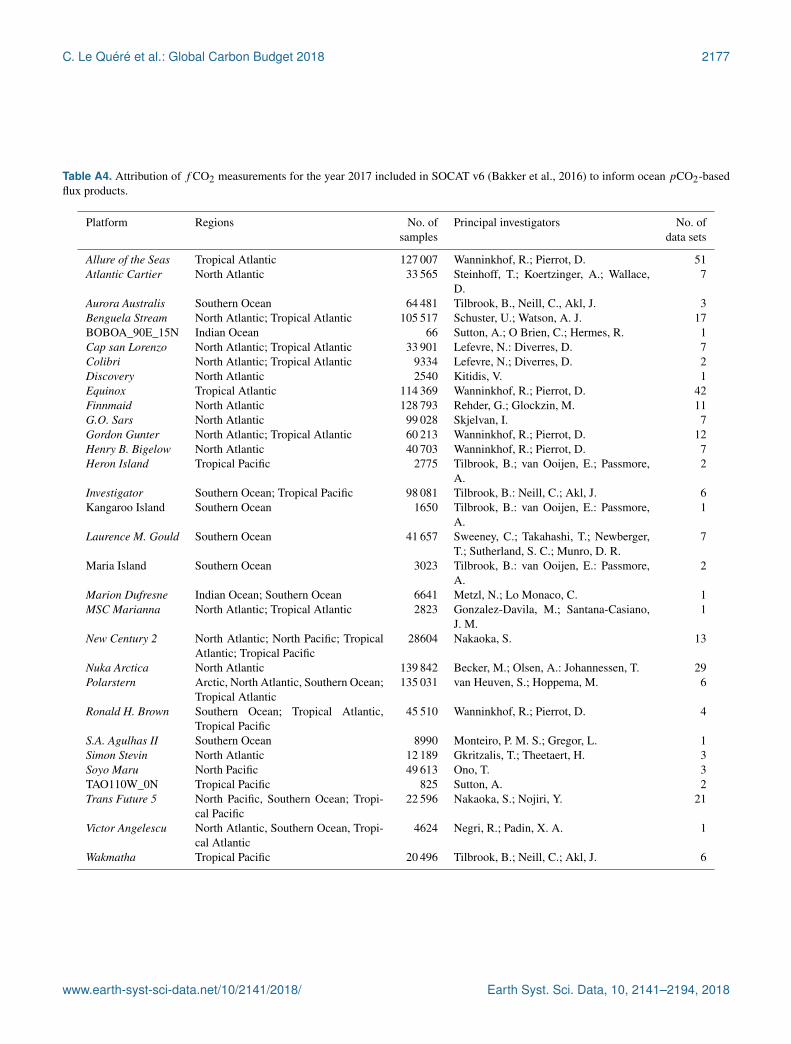
C. Le Quéré et al.: Global Carbon Budget 2018 2177
Table A4. Attribution of fCO2 measurements for the year 2017 included in SOCAT v6 (Bakker et al., 2016) to inform ocean pCO2-basedflux products.
Platform Regions No. of Principal investigators No. ofsamples data sets
Allure of the Seas Tropical Atlantic 127 007 Wanninkhof, R.; Pierrot, D. 51Atlantic Cartier North Atlantic 33 565 Steinhoff, T.; Koertzinger, A.; Wallace,
D.7
Aurora Australis Southern Ocean 64 481 Tilbrook, B., Neill, C., Akl, J. 3Benguela Stream North Atlantic; Tropical Atlantic 105 517 Schuster, U.; Watson, A. J. 17BOBOA_90E_15N Indian Ocean 66 Sutton, A.; O Brien, C.; Hermes, R. 1Cap san Lorenzo North Atlantic; Tropical Atlantic 33 901 Lefevre, N.: Diverres, D. 7Colibri North Atlantic; Tropical Atlantic 9334 Lefevre, N.; Diverres, D. 2Discovery North Atlantic 2540 Kitidis, V. 1Equinox Tropical Atlantic 114 369 Wanninkhof, R.; Pierrot, D. 42Finnmaid North Atlantic 128 793 Rehder, G.; Glockzin, M. 11G.O. Sars North Atlantic 99 028 Skjelvan, I. 7Gordon Gunter North Atlantic; Tropical Atlantic 60 213 Wanninkhof, R.; Pierrot, D. 12Henry B. Bigelow North Atlantic 40 703 Wanninkhof, R.; Pierrot, D. 7Heron Island Tropical Pacific 2775 Tilbrook, B.; van Ooijen, E.; Passmore,
A.2
Investigator Southern Ocean; Tropical Pacific 98 081 Tilbrook, B.: Neill, C.; Akl, J. 6Kangaroo Island Southern Ocean 1650 Tilbrook, B.: van Ooijen, E.: Passmore,
A.1
Laurence M. Gould Southern Ocean 41 657 Sweeney, C.; Takahashi, T.; Newberger,T.; Sutherland, S. C.; Munro, D. R.
7
Maria Island Southern Ocean 3023 Tilbrook, B.: van Ooijen, E.: Passmore,A.
2
Marion Dufresne Indian Ocean; Southern Ocean 6641 Metzl, N.; Lo Monaco, C. 1MSC Marianna North Atlantic; Tropical Atlantic 2823 Gonzalez-Davila, M.; Santana-Casiano,
J. M.1
New Century 2 North Atlantic; North Pacific; TropicalAtlantic; Tropical Pacific
28604 Nakaoka, S. 13
Nuka Arctica North Atlantic 139 842 Becker, M.; Olsen, A.: Johannessen, T. 29Polarstern Arctic, North Atlantic, Southern Ocean;
Tropical Atlantic135 031 van Heuven, S.; Hoppema, M. 6
Ronald H. Brown Southern Ocean; Tropical Atlantic,Tropical Pacific
45 510 Wanninkhof, R.; Pierrot, D. 4
S.A. Agulhas II Southern Ocean 8990 Monteiro, P. M. S.; Gregor, L. 1Simon Stevin North Atlantic 12 189 Gkritzalis, T.; Theetaert, H. 3Soyo Maru North Pacific 49 613 Ono, T. 3TAO110W_0N Tropical Pacific 825 Sutton, A. 2Trans Future 5 North Pacific, Southern Ocean; Tropi-
cal Pacific22 596 Nakaoka, S.; Nojiri, Y. 21
Victor Angelescu North Atlantic, Southern Ocean, Tropi-cal Atlantic
4624 Negri, R.; Padin, X. A. 1
Wakmatha Tropical Pacific 20 496 Tilbrook, B.; Neill, C.; Akl, J. 6
www.earth-syst-sci-data.net/10/2141/2018/ Earth Syst. Sci. Data, 10, 2141–2194, 2018

2178 C. Le Quéré et al.: Global Carbon Budget 2018
Table A5. Funding supporting the production of the various components of the global carbon budget in addition to the authors’ supportinginstitutions (see also acknowledgements).
Funder and grant number (where relevant) Author initials
Australia, Great Barrier Reef Foundation BT, CNAustralia, Integrated Marine Observing System (IMOS) BT, CNAustralian government National Environment Science Program (NESP) JGC, VHEC H2020 (AtlantOS: grant no. 633211) AO, USEC H2020 (CRESCENDO: grant no. 641816) MF, PF, RS, TIEC H2020 European Research Council (ERC) Synergy grant (IMBALANCE-P; grant no. ERC-2013-SyG-610028)
DSG
EC H2020 ERC (QUINCY; grant no. 647204). SZEC H2020 (RINGO: grant no. 730944; FixO3: grant no. 312463). USEC H2020 project (VERIFY: grant no. 776810) CLQ, GPP, IH, JIK, RMA, PP, PCFrench Institut National des Sciences de l’Univers (INSU) and Institut Polaire Français Paul-Emile Victor (IPEV), Sorbonne Universités (UPMC, Univ Paris 06)
NM
German Federal Ministry for Education and Research (BMBF) GR, MH, TSGerman Federal Ministry of Transport and Digital Infrastructure (BMVI) GR, MH, TSGerman Helmholtz Association in its ATMO programme AAGerman Helmholtz Association Innovation and Network Fund (VH-NG-1301) JHGerman Research Foundation’s Emmy Noether Programme (grant no. PO1751/1-1) JPIntegrated Carbon Observation System (ICOS) RI GR, MH, NL, TG, TJ, TS, IS, USFrench Institut de Recherche pour le Développement (IRD) NLJapan Environment Research and Technology Development Fund of the Ministry of the Envi-ronment (grant no. 2-1701)
PKP
Japan Fisheries Research and Education Agency (FREA), Ministry of Environment (MOE) TOJapan National Institute for Environmental Studies (NIES), Ministry of Environment (MOE) SNNetherlands Organization for Scientific Research (NWO; grant no. SH-312, 16666) IvdLLNorwegian Research Council (grant no. 229771) JSNorwegian Research Council (grant no. ICOS 245927) IS, TJ, BPNorwegian Research Council (grant no. 209701) RMA, JIK, GPPThe Netherlands, Research Foundation – Flanders (FWO contract no. G0H3317N) TGThe Copernicus Atmosphere Monitoring Service, implemented by the European Centre forMedium-Range Weather Forecasts (ECMWF) on behalf of the European Commission
FC
Swiss National Science Foundation (grant no. 200020_172476) SLUK BEIS/Defra Met Office Hadley Centre Climate Programme (grant no. GA01101) CDJUK Natural Environment Research Council (SONATA: grant no. NE/P021417/1) CLQ, USUK NERC (RAGNARoCC: grant no. NE/K002473/1) USUK Newton Fund, Met Office Climate Science for Service Partnership Brazil (CSSP Brazil) AWUS Climate Program Office of NOAA (grant no. NA13OAR4310219) LRU.S. Department of Agriculture, National Institute of Food and Agriculture (grant nos. 2015-67003-23489 and 2015-67003-23485)
DLL
U.S. Department of Commerce, NOAA/OAR’s Global Ocean Monitoring & Observing Pro-gram
AS, LB, DP
U.S. Department of Commerce, NOAA/OAR’s Ocean Acidification Program AS, DP, LBU.S. Department of Energy, Oak Ridge National Laboratory (contract no. DE-AC05-00OR22725)
APW
U.S. Department of Energy, Office of Science and BER programme (grant no. DE-SC0000016323)
ATJ
U.S. Department of Energy (grant nos. DE-FC03-97ER62402/A010 and DE-SC0012972) DLLUS NASA Interdisciplinary Research in Earth Science programme BPU.S. NASA (grant no. 80NSSC18K0897) SCD
Computing resources
Norway UNINETT Sigma2, National Infrastructure for High Performance Computing andData Storage in Norway (NN2980K/NS2980K)
JS
TGCC under allocations 2017-A0030102201 and 2017-A0030106328 made by GENCI FC, NVJapan National Institute for Environmental Studies computational resources EKUEA High Performance Computing Cluster, UK RW, CLQDeutsches Klimarechenzentrum (allocation bm0891) JEMSN, JP
Earth Syst. Sci. Data, 10, 2141–2194, 2018 www.earth-syst-sci-data.net/10/2141/2018/

C. Le Quéré et al.: Global Carbon Budget 2018 2179
Table A5. Continued.
Support for aircraft measurements in ObsPack
L. V. Gatti, M. Gloor, J. B. Miller: AMAZONICA consortium project was funded by NERC (NE/F005806/1), FAPESP(08/58120-3), GEOCARBON project (283080)Joshua DiGangi, NASA Langley Research Center, principal investigator of the airborne instrument that collected all of theCO2 observations during the Atmospheric Carbon and Transport – America campaigns.Observations from the Atmospheric Carbon and Transport (ACT) – America Earth Venture Suborbital mission were funded byNASA’s Earth Science Division (grant NNX15AG76G to Penn State)Jeff Peischl of the University of Colorado/CIRES for the NOAA WP-3D aircraft vertical profile data
www.earth-syst-sci-data.net/10/2141/2018/ Earth Syst. Sci. Data, 10, 2141–2194, 2018

2180 C. Le Quéré et al.: Global Carbon Budget 2018
Table A6. Aircraft measurement programmes archived by Cooperative Global Atmospheric Data Integration Project (CGADIP, 2017) thatcontribute to the evaluation of the atmospheric inversions (Fig. B3).
Measurement programme name in ObsPack Specific DOI Data providers
Airborne Aerosol Observatory, Bondville, Illinois Sweeney, C.; Dlugokencky, E. J.Alaska Coast Guard Sweeney, C.; McKain, K.; Karion, A.;
Dlugokencky, E. J.Atmospheric Carbon and Transport – America https://doi.org/10.3334/ORNLDAAC/1556 Davis, K. J.; Digangi, J. P.; Yang, M.Atmospheric Carbon and Transport – America Davis, K. J.; Sweeney, C.; Dlugo-
kencky, E. J.; Yang, M.Alta Floresta Gatti, L. V.; Gloor, E.; Miller, J. B.Aircraft observation of atmospheric trace gases by JMA [email protected], Radiation, and Cloud Processes affecting ArcticClimate 2008 (air campaign)
Ryerson, T. B.; Peischl, J.; Aikin, K. C.
LARC – NASA Langley Research Center AircraftCampaign
Chen, G.; Digangi, J. P.
Beaver Crossing, Nebraska Sweeney, C.; Dlugokencky, E. J.California Nexus 2010 (air campaign) Ryerson, T. B.; Peischl, J.; Aikin, K. C.Briggsdale, Colorado Sweeney, C.; Dlugokencky, E. J.Cape May, New Jersey Sweeney, C.; Dlugokencky, E. J.CONTRAIL (Comprehensive Observation Network forTRace gases by AIrLiner)
https://doi.org/10.17595/20180208.001 Machida, T.; Matsueda, H.; Sawa, Y.;Niwa, Y.
Carbon in Arctic Reservoirs Vulnerability Experiment(CARVE)
Sweeney, C.; Karion, A.; Miller, J. B.;Miller, C. E.; Dlugokencky, E. J.
LARC – NASA Langley Research Center AircraftCampaign
Chen, G.; Digangi, J. P.; Beyersdorf, A.
LARC – NASA Langley Research Center AircraftCampaign
Chen, G.; Digangi, J. P.; Yang, M.
Dahlen, North Dakota Sweeney, C.; Dlugokencky, E. J.Estevan Point, British Columbia Sweeney, C.; Dlugokencky, E. J.East Trout Lake, Saskatchewan Sweeney, C.; Dlugokencky, E. J.Molokai Island, Hawaii Sweeney, C.; Dlugokencky, E. J.Homer, Illinois Sweeney, C.; Dlugokencky, E. J.HIPPO (HIAPER Pole-to-Pole Observations) https://doi.org/10.3334/CDIAC/HIPPO_010 Wofsy, S. C.; Stephens, B. B.; Elkins, J.
W.; Hintsa, E. J.; Moore, F.INFLUX (Indianapolis Flux Experiment) Sweeney, C.; Dlugokencky, E. J.; Shep-
son, P. B.; Turnbull, J.Park Falls, Wisconsin Sweeney, C.; Dlugokencky, E. J.Mid-Continent Intensive Campaign Sweeney, C.; Dlugokencky, E. J.Marcellus, Pennsylvania Sweeney, C.; Dlugokencky, E. J.Worcester, Massachusetts Sweeney, C.; Dlugokencky, E. J.ORCAS (O2/N2 Ratio and CO2 Airborne Southern OceanStudy)
https://doi.org/10.5065/D6SB445X Stephens, B. B.; Sweeney, C.; McKain,K.; Kort, E. A.
Poker Flat, Alaska Sweeney, C.; Dlugokencky, E. J.Rio Branco Gatti, L. V.; Gloor, E.; Miller, J. B.Rarotonga Sweeney, C.; Dlugokencky, E. J.Montzka Sweeney, C.; Dlugokencky, E. J.Santarem Sweeney, C.; Dlugokencky, E. J.Charleston, South Carolina Sweeney, C.; Dlugokencky, E. J.LARC – NASA Langley Research Center AircraftCampaign
Chen, G.; Digangi, J. P.; Beyersdorf, A.
Southeast Nexus 2013 (air campaign) Ryerson, T. B.; Peischl, J.; Aikin, K. C.Southern Great Plains, Oklahoma Sweeney, C.; Dlugokencky, E. J.; Bi-
raud, S.Shale Oil and Natural Gas Nexus 2015 (air campaign) Ryerson, T. B.; Peischl, J.; Aikin, K. C.Harvard University aircraft campaign Wofsy, S. C.Tabatinga Gatti, L. V.; Gloor, E.; Miller, J. B.Sinton, Texas Sweeney, C.; Dlugokencky, E. J.Trinidad Head, California Sweeney, C.; Dlugokencky, E. J.Atmospheric Tomography Mission (ATom) McKain, K.; Sweeney, C.Ulaanbaatar Sweeney, C.; Dlugokencky, E. J.West Branch, Iowa Sweeney, C.; Dlugokencky, E. J.
Earth Syst. Sci. Data, 10, 2141–2194, 2018 www.earth-syst-sci-data.net/10/2141/2018/

C. Le Quéré et al.: Global Carbon Budget 2018 2181
Appendix B: Supplementary figures
Figure B1. Evaluation of the GOBMs and flux products using the interannual mismatch metric for the period from 1985 to 2017, asproposed by Rödenbeck et al. (2015) and the SOCAT v6 database, versus the amplitude of the annual variability (taken as the annual standarddeviation). Results are presented for the globe, north (> 30◦ N), tropics (30◦ S–30◦ N), and south (< 30◦ S) for the GOBMs (circles) andfor the pCO2-based flux products (star symbols). The two pCO2-based flux products use the SOCAT database and therefore are not fullyindependent from the data (see Sect. 2.5.1).
www.earth-syst-sci-data.net/10/2141/2018/ Earth Syst. Sci. Data, 10, 2141–2194, 2018

2182 C. Le Quéré et al.: Global Carbon Budget 2018
Figure B2. Evaluation of the DGVM using the International Land Model Benchmarking system (ILAMB; Collier et al., 2018) (left) absoluteskill scores and (right) skill scores relative to other models. The benchmarking is carried out with observations for vegetation biomass (Saatchiet al., 2011; GlobalCarbon, unpublished data; Avitabile et al., 2016), GPP (Jung et al., 2010; Lasslop et al., 2010), leaf area index (De Kauweet al., 2011; Myneni et al., 1997), net ecosystem exchange (Jung et al., 2010; Lasslop et al., 2010), ecosystem respiration (Jung et al., 2010;Lasslop et al., 2010), soil carbon (Hugelius et al., 2013; Todd-Brown et al., 2013), evapotranspiration (De Kauwe et al., 2011), and runoff(Dai and Trenberth, 2002). For each model–observation comparison a series of error metrics are calculated, scores are then calculated as anexponential function of each error metric, and finally for each variable the multiple scores from different metrics and observational data setsare combined to give the overall variable scores shown in the left panel. The set of error metrics vary with data set and can include metricsbased on the period mean, bias, root-mean-squared error, spatial distribution, interannual variability, and seasonal cycle. The relative skillscore shown in the right panel is a Z score, which indicates in units of standard deviation the model scores relative to the multi-model meanscore for a given variable. Grey boxes represent missing model data.
Earth Syst. Sci. Data, 10, 2141–2194, 2018 www.earth-syst-sci-data.net/10/2141/2018/

C. Le Quéré et al.: Global Carbon Budget 2018 2183
Figure B3. Evaluation of the atmospheric inversion products. The mean of the absolute model minus observations is shown for four latitudebands. The four models are compared to independent CO2 measurements made onboard aircraft over many places of the world between 1 and7 km above sea level. All data between 2008 and 2016 archived in the Cooperative Global Atmospheric Data Integration Project (CGADIP,2017) have been used to compute the biases of the differences in four 45◦ latitude bins. Land and ocean data are used without distinction.The number of data for each latitude band is 16 000 (90–45◦ S), 53 000 (45◦ S–0), 64 000 (0–45◦ N), and 122 000 (45–90◦ N), rounded offto the nearest thousand.
www.earth-syst-sci-data.net/10/2141/2018/ Earth Syst. Sci. Data, 10, 2141–2194, 2018

2184 C. Le Quéré et al.: Global Carbon Budget 2018
Figure B4. Comparison of global carbon budget components released annually by GCP since 2006. CO2 emissions from (a) fossil CO2emissions (EFF) and (b) land-use change (ELUC), as well as their partitioning among (c) the atmosphere (GATM), (d) the land (SLAND), and(e) the ocean (SOCEAN). See legend for the corresponding years and Table 3 for references. The budget year corresponds to the year whenthe budget was first released. All values are in GtC yr−1. Grey shading shows the uncertainty bounds representing ±1σ of the current globalcarbon budget.
Earth Syst. Sci. Data, 10, 2141–2194, 2018 www.earth-syst-sci-data.net/10/2141/2018/
C. Le Quéré et al.: Global Carbon Budget 2018 2185
Author contributions. CLQ, RMA, PF, SS, JH, JP, GPP, JGC,and WP designed the study, conducted the analysis, and wrote thepaper. RMA and GPP produced the emissions and their uncertain-ties, 2018 emission projections, and analysed the emissions data.RMA, JIK, GPP, ZL, and BZ produced the 2018 projection forChina’s emissions and its uncertainty. RFK and PPT provided keyatmospheric CO2 data. RMA and CDJ produced the 2018 projec-tion for atmospheric CO2 growth rate and its uncertainty. FC, PPa,CR, and IvdLL provided an updated atmospheric inversion, devel-oped the protocol and produced the evaluation. AB and RAH pro-vided updated land-use change emissions. LPC, GH, KKG, FNT,and GRvdW provided forcing data for land-use change. AA, VKA,DSG, VH, AKJ, EK, SL, DL, JEMSN, PPe, BPo, MR, HT, APW,AJW and SZ provided an update of a DGVM. IH and NV providedforcing data for the DGVMs. FMH and ER provided the evalua-tion of the DGVMs. JH, LBo, SCD, TI, JS, RS and RW providedan update of a GOBM. PL and CR provided an update of an oceanflux product. Lba, TG, MH, TJ, NL, NM, DRM, SN, CN, AO, TO,BPf, DP, GR, US, IS, TS, AS and BT provided ocean pCO2 mea-surements for the year 2017. LR provided an updated river flux es-timate. CLQ, PAP, RMA and AP revised the figures, tables, textand/or numbers to ensure the update is clear from the 2017 editionand in phase with the globalcarbonatlas.org.
Competing interests. The authors declare that they have no con-flict of interest.
Acknowledgements. We thank all people and institutions whoprovided the data used in this carbon budget; Richard Betts, ErikBuitenhuis, Jinfeng Chang, Shijie Shu, and Naomi Smith for theirinvolvement in the development, use and analysis of the modelsand data products used here; and Fortunat Joos, Samar Khatiwala,and Timothy DeVries for providing historical data. We thank RobJackson and the Global Carbon Project members for their inputthroughout the development of this update. We thank Ed Dlugo-kencky for providing atmospheric CO2 measurements; Camilla Ste-gen Landa, Christophe Bernard, and Steve Jones of the BjerknesClimate Data Centre and the ICOS Ocean Thematic Centre datamanagement at the University of Bergen, who helped with gather-ing information from the SOCAT community; and Vassilis Kitidis,Pedro M. S. Monteiro, Luke Gregor, Melchor Gonzáles-Dávila, J.Magdalena Santana-Casiano, Ruben Negri, and X. Antonio Padin,who contributed to the provision of ocean pCO2 observations (seeTable A1). This is NOAA-PMEL contribution number 4847. Wethank the institutions and funding agencies responsible for the col-lection and quality control of the data included in SOCAT and thesupport of the International Ocean Carbon Coordination Project(IOCCP), the Surface Ocean–Lower Atmosphere Study (SOLAS),and the Integrated Marine Biogeochemistry and Ecosystem Re-search (IMBER) programme. We thank the FAO and its membercountries for the collection and free dissemination of data relevantto this work. We thank data providers ObsPack GLOBALVIEW-plus v1.0 and NRT v3.0 for atmospheric CO2 observations used inCTE2016-FT and the following people for sharing their aircraft dataused in Fig. B3: Toshinobu Machida, Guangsheng Chen, StevenC. Wofsy, Ken Davis, Joshua DiGangi, Jeff Peischl, Thomas B.Ryerson, Britton Stephens, Colm Sweeney, Kathryn McKain, and
Luciana V. Gatti; University of Colorado/CIRES for the NOAAWP-3D aircraft vertical profile data; and the Japan MeteorologicalAgency. We thank the individuals and institutions that provided thedatabases used for the model evaluations introduced here and NigelHawtin for producing Fig. 2.
Finally, we thank all funders who have supported the individualand joint contributions to this work (see Table A5), as well asthe reviewers of this paper and previous versions, and the manyresearchers who have provided feedback.
Edited by: David CarlsonReviewed by: H. Damon Matthews, Albertus J. Dolman,and one anonymous referee
References
Andres, R. J., Boden, T. A., Bréon, F.-M., Ciais, P., Davis, S.,Erickson, D., Gregg, J. S., Jacobson, A., Marland, G., Miller,J., Oda, T., Olivier, J. G. J., Raupach, M. R., Rayner, P.,and Treanton, K.: A synthesis of carbon dioxide emissionsfrom fossil-fuel combustion, Biogeosciences, 9, 1845–1871,https://doi.org/10.5194/bg-9-1845-2012, 2012.
Andres, R. J., Boden, T., and Higdon, D.: A new evalua-tion of the uncertainty associated with CDIAC estimates offossil fuel carbon dioxide emission, Tellus B, 66, 23616,https://doi.org/10.3402/tellusb.v66.23616, 2014.
Andrew, R. M.: Global CO2 emissions from cement production,Earth Syst. Sci. Data, 10, 195–217, https://doi.org/10.5194/essd-10-195-2018, 2018.
Andrew, R. M. and Peters, G. P.: A multi-region input-output table based on the Global Trade Analysis ProjectDatabase (GTAP-MRIO), Econ. Syst. Res., 25, 99–121,https://doi.org/10.1080/09535314.2012.761953, 2013.
Archer, D., Eby, M., Brovkin, V., Ridgwell, A., Cao, L., Miko-lajewicz, U., Caldeira, K. M., K., Munhoven, G., Montene-gro, A., and Tokos, K.: Atmospheric Lifetime of Fossil FuelCarbon Dioxide, Annu. Rev. Earth Pl. Sc., 37, 117–134,https://doi.org/10.1146/annurev.earth.031208.100206, 2009.
Arneth, A., Sitch, S., Pongratz, J., Stocker, B. D., Ciais, P., Poulter,B., Bayer, A. D., Bondeau, A., Calle, L., Chini, L. P., Gasser,T., Fader, M., Friedlingstein, P., Kato, E., Li, W., Lindeskog, M.,Nabel, J. E. M. S., Pugh, T. A. M., Robertson, E., Viovy, N., Yue,C., and Zaehle, S.: Historical carbon dioxide emissions caused byland-use changes are possibly larger than assumed, Nat. Geosci.,10, 79–84, https://doi.org/10.1038/ngeo2882, 2017.
Arora, V. K., Boer, G. J., Christian, J. R., Curry, C. L., Denman,K. L., Zahariev, K., Flato, G. M., Scinocca, J. F., Merryfield,W. J., and Lee, W. G.: The Effect of Terrestrial Photosynthe-sis Down Regulation on the Twentieth-Century Carbon BudgetSimulated with the CCCma Earth System Model, J. Climate, 22,6066–6088, https://doi.org/10.1175/2009jcli3037.1, 2009.
Aumont, O. and Bopp, L.: Globalizing results from ocean in situiron fertilization studies, Global Biogeochem. Cy., 20, GB2017,https://doi.org/10.1029/2005GB002591, 2006.
Avitabile, V., Herold, M., Heuvelink, G. B. M., Lewis, S. L.,Phillips, O. L., Asner, G. P., Armston, J., Ashton, P. S., Banin, L.,Bayol, N., Berry, N. J., Boeckx, P., de Jong, B. H. J., DeVries, B.,Girardin, C. A. J., Kearsley, E., Lindsell, J. A., Lopez-Gonzalez,
www.earth-syst-sci-data.net/10/2141/2018/ Earth Syst. Sci. Data, 10, 2141–2194, 2018

2186 C. Le Quéré et al.: Global Carbon Budget 2018
G., Lucas, R., Malhi, Y., Morel, A., Mitchard, E. T. A., Nagy, L.,Qie, L., Quinones, M. J., Ryan, C. M., Ferry, S. J. W., Sunder-land, T., Laurin, G. V., Gatti, R. C., Valentini, R., Verbeeck, H.,Wijaya, A., and Willcock, S.: An integrated pan-tropical biomassmap using multiple reference datasets, Glob. Change Biol., 22,1406–1420, https://doi.org/10.1111/gcb.13139, 2016.
Baccini, A., Walker, W., Carvalho, L., Farina, M., Sulla-Menashe,D., and Houghton, R. A.: Tropical forests are a net carbon sourcebased on aboveground measurements of gain and loss, Science,358, 230–233, https://doi.org/10.1126/science.aam5962, 2017.
Bakker, D. C. E., Pfeil, B., Landa, C. S., Metzl, N., O’Brien, K.M., Olsen, A., Smith, K., Cosca, C., Harasawa, S., Jones, S. D.,Nakaoka, S.-I., Nojiri, Y., Schuster, U., Steinhoff, T., Sweeney,C., Takahashi, T., Tilbrook, B., Wada, C., Wanninkhof, R., Alin,S. R., Balestrini, C. F., Barbero, L., Bates, N. R., Bianchi, A. A.,Bonou, F., Boutin, J., Bozec, Y., Burger, E. F., Cai, W.-J., Castle,R. D., Chen, L., Chierici, M., Currie, K., Evans, W., Feather-stone, C., Feely, R. A., Fransson, A., Goyet, C., Greenwood, N.,Gregor, L., Hankin, S., Hardman-Mountford, N. J., Harlay, J.,Hauck, J., Hoppema, M., Humphreys, M. P., Hunt, C. W., Huss,B., Ibánhez, J. S. P., Johannessen, T., Keeling, R., Kitidis, V.,Körtzinger, A., Kozyr, A., Krasakopoulou, E., Kuwata, A., Land-schützer, P., Lauvset, S. K., Lefèvre, N., Lo Monaco, C., Manke,A., Mathis, J. T., Merlivat, L., Millero, F. J., Monteiro, P. M. S.,Munro, D. R., Murata, A., Newberger, T., Omar, A. M., Ono, T.,Paterson, K., Pearce, D., Pierrot, D., Robbins, L. L., Saito, S.,Salisbury, J., Schlitzer, R., Schneider, B., Schweitzer, R., Sieger,R., Skjelvan, I., Sullivan, K. F., Sutherland, S. C., Sutton, A. J.,Tadokoro, K., Telszewski, M., Tuma, M., van Heuven, S. M. A.C., Vandemark, D., Ward, B., Watson, A. J., and Xu, S.: A multi-decade record of high-quality fCO2 data in version 3 of the Sur-face Ocean CO2 Atlas (SOCAT), Earth Syst. Sci. Data, 8, 383–413, https://doi.org/10.5194/essd-8-383-2016, 2016.
Ballantyne, A. P., Alden, C. B., Miller, J. B., Tans, P. P., and White,J. W. C.: Increase in observed net carbon dioxide uptake byland and oceans during the last 50 years, Nature, 488, 70–72,https://doi.org/10.1038/nature11299, 2012.
Ballantyne, A. P., Andres, R., Houghton, R., Stocker, B. D., Wan-ninkhof, R., Anderegg, W., Cooper, L. A., DeGrandpre, M.,Tans, P. P., Miller, J. B., Alden, C., and White, J. W. C.: Au-dit of the global carbon budget: estimate errors and their im-pact on uptake uncertainty, Biogeosciences, 12, 2565–2584,https://doi.org/10.5194/bg-12-2565-2015, 2015.
Bauer, J. E., Cai, W.-J., Raymond, P. A., Bianchi, T. S.,Hopkinson, C. S., and Regnier, P. A. G.: The changingcarbon cycle of the coastal ocean, Nature, 504, 61–70,https://doi.org/10.1038/nature12857, 2013.
Berthet, S., Séférian, R., Bricaud, C., Chevallier, M., Voldoire, A.,and Ethé, C.: On the benefits of increasing resolution for biogeo-chemistry climate modelling, J. Adv. Model. Earth Sy., submit-ted, 2018.
Betts, R. A., Jones, C. D., Knight, J. R., Keeling, R. F., and Kennedy,J. J.: El Nino and a record CO2 rise, Nat. Clim. Change, 6, 806–810, https://doi.org/10.1038/nclimate3063, 2016.
Boden, T. A., Marland, G., and Andres, R. J.: Global, Re-gional, and National Fossil-Fuel CO2 Emissions, available at:http://cdiac.ornl.gov/trends/emis/overview_2014.html (last ac-cess: July 2017), Oak Ridge National Laboratory, U.S. Depart-ment of Energy, Oak Ridge, Tenn., USA, 2017.
BP: BP Statistical Review of World Energy June 2018,available at: https://www.bp.com/content/dam/bp/en/corporate/pdf/energy-economics/statistical-review/bp-stats-review-2018-full-report.pdf, last access: June 2018.
Bruno, M. and Joos, F.: Terrestrial carbon storage during the past200 years: A monte carlo analysis of CO2 data from ice core andatmospheric measurements, Global Biogeochem. Cy., 11, 111–124, https://doi.org/10.1029/96GB03611, 1997.
Buitenhuis, E. T., Rivkin, R. B., Sailley, S., and LeQuéré, C.: Biogeochemical fluxes through micro-zooplankton, Global Biogeochem. Cy., 24, GB4015,https://doi.org/10.1029/2009GB003601, 2010.
Canadell, J. G., Le Quéré, C., Raupach, M. R., Field, C. B., Buiten-huis, E. T., Ciais, P., Conway, T. J., Gillett, N. P., Houghton, R.A., and Marland, G.: Contributions to accelerating atmosphericCO2 growth from economic activity, carbon intensity, and effi-ciency of natural sinks, P. Natl. Acad. Sci. USA, 104, 18866–18870, https://doi.org/10.1073/pnas.0702737104, 2007.
Carbontracker Team: Compilation of near real time atmo-spheric carbon dioxide data provided by NOAA and EC,obspack_co2_1_NRT_v3.3_2017-04-19; NOAA Earth Sys-tem Research Laboratory, Global Monitoring Division,https://doi.org/10.15138/G3G01J, 2017.
CEA: Central Electricity Authority (CEA), 2018: Daily Coal –Archive, Central Electricity Authority, available at: http://www.cea.nic.in/dailyarchive.html, last access: 7 November 2018.
CGADIP: Cooperative Global Atmospheric Data IntegrationProject (2017), Multi-laboratory compilation of atmo-spheric carbon dioxide data for the period 1957–2016;obspack_co2_1_GLOBALVIEWplus_v3.2_2017-11-02 [Dataset], NOAA Earth System Research Laboratory, Global Moni-toring Division, 2017.
Chatfield, C.: The Holt-Winters Forecasting Procedure, J. Roy. Stat.Soc. C-Appl., 27, 264–279, https://doi.org/10.2307/2347162,1978.
Chevallier, F., Fisher, M., Peylin, P., Serrar, S., Bousquet,P., Bréon, F.-M., Chédin, A., and Ciais, P.: Inferring CO2sources and sinks from satellite observations: Method andapplication to TOVS data, J. Geophys. Res., 110, D24309,https://doi.org/10.1029/2005JD006390, 2005.
Ciais, P., Sabine, C., Govindasamy, B., Bopp, L., Brovkin, V.,Canadell, J., Chhabra, A., DeFries, R., Galloway, J., Heimann,M., Jones, C., Le Quéré, C., Myneni, R., Piao, S., and Thorn-ton, P.: Chapter 6: Carbon and Other Biogeochemical Cycles,in: Climate Change 2013 The Physical Science Basis, edited by:Stocker, T., Qin, D., and Platner, G.-K., Cambridge UniversityPress, Cambridge, 2013.
CIL: Coal India Limited, 2018: Production and Offtake Perfor-mance of CIL and Subsidiary Companies, available at: https://www.coalindia.in/en-us/performance/physical.aspx, last access:1 November 2018.
Clark, D. B., Mercado, L. M., Sitch, S., Jones, C. D., Gedney, N.,Best, M. J., Pryor, M., Rooney, G. G., Essery, R. L. H., Blyth,E., Boucher, O., Harding, R. J., Huntingford, C., and Cox, P.M.: The Joint UK Land Environment Simulator (JULES), modeldescription – Part 2: Carbon fluxes and vegetation dynamics,Geosci. Model Dev., 4, 701–722, https://doi.org/10.5194/gmd-4-701-2011, 2011.
Earth Syst. Sci. Data, 10, 2141–2194, 2018 www.earth-syst-sci-data.net/10/2141/2018/

C. Le Quéré et al.: Global Carbon Budget 2018 2187
Collier, N., Hoffman, F. M., Lawrence, D. M., Keppel-Aleks, G.,Koven, C. D., Riley, W. J., Mu, M., and Randerson, J. T.: TheInternational Land Model Benchmarking (ILAMB) System: De-sign, Theory, and Implementation, J. Adv. Model. Earth Sy., 10,https://doi.org/10.1029/2018MS001354, 2018.
Cox, P. M., Pearson, D., Booth, B. B., Friedlingstein, P., Hunting-ford, C., Jones, C. D., and Luke, C. M.: Sensitivity of tropicalcarbon to climate change constrained by carbon dioxide variabil-ity, Nature, 494, 341–344, https://doi.org/10.1038/nature11882,2013.
Dai, A. and Trenberth, K. E.: Estimates of freshwater dis-charge from continents: Latitudinal and seasonal variations,J. Hydrometeorol., 3, 660–687, https://doi.org/10.1175/1525-7541(2002)003<0660:EOFDFC>2.0.CO;2, 2002.
Davis, S. J. and Caldeira, K.: Consumption-based accounting ofCO2 emissions, P. Natl. Acad. Sci. USA, 107, 5687–5692,https://doi.org/10.1073/pnas.0906974107, 2010.
De Kauwe, M. G., Disney, M. I., Quaife, T., Lewis, P.,and Williams, M.: An assessment of the MODIS collec-tion 5 leaf area index product for a region of mixedconiferous forest, Remote Sens. Environ., 115, 767–780,https://doi.org/10.1016/j.rse.2010.11.004, 2011.
Denman, K. L., Brasseur, G., Chidthaisong, A., Ciais, P., Cox, P. M.,Dickinson, R. E., Hauglustaine, D., Heinze, C., Holland, E., Ja-cob, D., Lohmann, U., Ramachandran, S., Leite da Silva Dias, P.,Wofsy, S. C., and Zhang, X.: Couplings Between Changes in theClimate System and Biogeochemistry, in: Climate Change 2007:The Physical Science Basis. Contribution of Working Group Ito the Fourth Assessment Report of the Intergovernmental Panelon Climate Change, edited by: Solomon, S., Qin D., ManningM., Marquis M., Averyt K., Tignor M. M. B., Miller, H. L., andChen Z. L., Cambridge University Press, Cambridge, UK andNew York, USA, 499–587, 2007.
DeVries, T.: The oceanic anthropogenic CO2 sink: Stor-age, air-sea fluxes, and transports over the indus-trial era, Global Biogeochem. Cy., 28, 631–647,https://doi.org/10.1002/2013GB004739, 2014.
DeVries, T., Holzer, M., and Primeau, F.: Recent increase in oceaniccarbon uptake driven by weaker upper-ocean overturning, Na-ture, 542, 215–218, https://doi.org/10.1038/nature21068, 2017.
Dlugokencky, E. and Tans, P.: Trends in atmospheric carbon diox-ide, National Oceanic & Atmospheric Administration, Earth Sys-tem Research Laboratory (NOAA/ESRL), available at: http://www.esrl.noaa.gov/gmd/ccgg/trends/global.html, last access: 4September 2018.
Doney, S. C., Lima, I., Feely, R. A., Glover, D. M., Lindsay,K., Mahowald, N., Moore, J. K., and Wanninkhof, R.: Mech-anisms governing interannual variability in upper-ocean inor-ganic carbon system and air–sea CO2 fluxes: Physical cli-mate and atmospheric dust, Deep-Sea Res. Pt. II, 56, 640–655,https://doi.org/10.1016/j.dsr2.2008.12.006, 2009.
Duce, R. A., LaRoche, J., Altieri, K., Arrigo, K. R., Baker, A.R., Capone, D. G., Cornell, S., Dentener, F., Galloway, J.,Ganeshram, R. S., Geider, R. J., Jickells, T., Kuypers, M. M.,Langlois, R., Liss, P. S., Liu, S. M., Middelburg, J. J., Moore,C. M., Nickovic, S., Oschlies, A., Pedersen, T., Prospero, J.,Schlitzer, R., Seitzinger, S., Sorensen, L. L., Uematsu, M., Ul-loa, O., Voss, M., Ward, B., and Zamora, L.: Impacts of atmo-
spheric anthropogenic nitrogen on the open ocean, Science, 320,893–897, https://doi.org/10.1126/science.1150369, 2008.
Dufour, C. O., Le Sommer, J., Gehlen, M., Orr, J. C., Molines, J.M., Simeon, J., and Barnier, B.: Eddy compensation and controlsof the enhanced sea-to-air CO2 flux during positive phases of theSouthern Annular Mode, Global Biogeochem. Cy., 27, 950–961,https://doi.org/10.1002/gbc.20090, 2013.
Durant, A. J., Le Quéré, C., Hope, C., and Friend, A. D.: Eco-nomic value of improved quantification in global sources andsinks of carbon dioxide, Philos. T. Roy Soc. A, 269, 1967–1979,https://doi.org/10.1098/rsta.2011.0002, 2011.
EIA: U.S. Energy Information Administration, Short-Term En-ergy and Winter Fuels Outlook, available at: http://www.eia.gov/forecasts/steo/outlook.cfm, last access: 7 November 2018.
ENTSO-E: The European Network of Transmission System Op-erators Electricity Transparency Platform, available at: https://transparency.entsoe.eu/, last access: 1 November 2018.
Erb, K.-H., Kastner, T., Luyssaert, S., Houghton, R. A., Kuem-merle, T., Olofsson, P., and Haberl, H.: Bias in the attribu-tion of forest carbon sinks, Nat. Clim. Change, 3, 854–856,https://doi.org/10.1038/nclimate2004, 2013.
Etheridge, D. M., Steele, L. P., Langenfelds, R. L., and Francey,R. J.: Natural and anthropogenic changes in atmospheric CO2over the last 1000 years from air in Antarctic ice and firn, J. Geo-phys. Res., 101, 4115–4128, https://doi.org/10.1029/95JD03410,1996.
Eurostat: Supply and transformation of solid fuels – monthlydata (nrg_101m), available at: https://ec.europa.eu/eurostat/data/database, last access: 7 November 2018.
FAO: Global Forest Resources Assessment 2015, Food and Agri-culture Organization of the United Nations, Rome, Italy, 2015.
FAOSTAT: Food and Agriculture Organization Statistics Division,available at: http://faostat.fao.org/, last access: 2015.
Figueres, C., Whiteman, G., Le Quéré, C., and Peters, G. P.: Carbonemissions rise again, Nature, 564, 27–31, 2018.
Francey, R. J., Trudinger, C. M., van der Schoot, M., Law, R. M.,Krummel, P. B., Langenfelds, R. L., Steele, L. P., Allison, C.E., Stavert, A. R., Andres, R. J., and Rodenbeck, C.: Reply to“Anthropogenic CO2 emissions”, Nat. Clim. Change, 3, p. 604,https://doi.org/10.1038/nclimate1925, 2013.
Friedlingstein, P., Houghton, R. A., Marland, G., Hackler, J., Boden,T. A., Conway, T. J., Canadell, J. G., Raupach, M. R., Ciais, P.,and Le Quéré, C.: Update on CO2 emissions, Nat. Geosci., 3,811–812, https://doi.org/10.1038/ngeo1022, 2010.
Friedlingstein, P., Andrew, R. M., Rogelj, J., Peters, G. P., Canadell,J. G., Knutti, R., Luderer, G., Raupach, M. R., Schaeffer, M., vanVuuren, D. P., and Le Quéré, C.: Persistent growth of CO2 emis-sions and implications for reaching climate targets, Nat. Geosci.,7, 709–715, https://doi.org/10.1038/NGEO2248, 2014.
Gasser, T., Ciais, P., Boucher, O., Quilcaille, Y., Tortora, M., Bopp,L., and Hauglustaine, D.: The compact Earth system model OS-CAR v2.2: description and first results, Geosci. Model Dev., 10,271–319, https://doi.org/10.5194/gmd-10-271-2017, 2017.
Gaubert, B., Stephens, B. B., Basu, S., Chevallier, F., Deng, F., Kort,E. A., Patra, P. K., Peters, W., Rödenbeck, C., Saeki, T., Schimel,D., Van der Laan-Luijkx, I., Wofsy, S., and Yin, Y.: Global atmo-spheric CO2 inverse models converging on neutral tropical landexchange but diverging on fossil fuel and atmospheric growth
www.earth-syst-sci-data.net/10/2141/2018/ Earth Syst. Sci. Data, 10, 2141–2194, 2018

2188 C. Le Quéré et al.: Global Carbon Budget 2018
rate, Biogeosciences Discuss., https://doi.org/10.5194/bg-2018-384, in review, 2018.
GCP: The Global Carbon Budget 2007, available at: http://www.globalcarbonproject.org/carbonbudget/archive.htm (last access:7 November 2016), 2007.
General Administration of Customs of the People’s Republic ofChina: Monthly statistical reports, available at: http://www.customs.gov.cn/customs/302249/302274/302277/index.html,last access: 15 November 2018.
Giglio, L., Schroeder, W., and Justice, C. O.: The col-lection 6 MODIS active fire detection algorithm andfire products, Remote Sens. Environ., 178, 31–41,https://doi.org/10.1016/j.rse.2016.02.054, 2016.
Gitz, V. and Ciais, P.: Amplifying effects of land-use change on fu-ture atmospheric CO2 levels, Global Biogeochem. Cy., 17, 1024,https://doi.org/10.1029/2002GB001963, 2003.
Global Carbon Project: Supplemental data of Global Carbon Bud-get 2018 (Version 1.1) [Data set], Global Carbon Project,https://doi.org/10.18160/GCP-2018, 2018.
Global Trade, Assistance, and Production: The GTAP 9 Data Base,available at: https://www.gtap.agecon.purdue.edu/databases/v9/default.asp, last access: September 2015.
GLOBALVIEW: Cooperative Global Atmospheric Data In-tegration Project (2016): Multi-laboratory compilation ofatmospheric carbon dioxide data for the period 1957–2015; obspack_co2_1_GLOBALVIEWplus_v2.1_2016_09_02;NOAA Earth System Research Laboratory, Global MonitoringDivision, https://doi.org/10.15138/G3059Z, 2016.
Goll, D. S., Vuichard, N., Maignan, F., Jornet-Puig, A., Sar-dans, J., Violette, A., Peng, S., Sun, Y., Kvakic, M., Guim-berteau, M., Guenet, B., Zaehle, S., Penuelas, J., Janssens, I.,and Ciais, P.: A representation of the phosphorus cycle for OR-CHIDEE (revision 4520), Geosci. Model Dev., 10, 3745–3770,https://doi.org/10.5194/gmd-10-3745-2017, 2017.
Gregg, J. S., Andres, R. J., and Marland, G.: China: Emissionspattern of the world leader in CO2 emissions from fossil fuelconsumption and cement production, Geophys. Res. Lett., 35,L08806, https://doi.org/10.1029/2007GL032887, 2008.
Hansis, E., Davis, S. J., and Pongratz, J.: Relevance ofmethodological choices for accounting of land use changecarbon fluxes, Global Biogeochem. Cy., 29, 1230–1246,https://doi.org/10.1002/2014GB004997, 2015.
Harris, I., Jones, P. D., Osborn, T. J., and Lister, D. H.: Up-dated high-resolution grids of monthly climatic observations– the CRU TS3.10 Dataset, Int. J. Climatol., 34, 623–642,https://doi.org/10.1002/joc.3711, 2014.
Hauck, J., Kohler, P., Wolf-Gladrow, D., and Volker, C.: Ironfertilisation and century-scale effects of open ocean disso-lution of olivine in a simulated CO2 removal experiment,Environ. Res. Lett., 11, 024007, https://doi.org/10.1088/1748-9326/11/2/024007, 2016.
Haverd, V., Smith, B., Nieradzik, L., Briggs, P. R., Woodgate, W.,Trudinger, C. M., Canadell, J. G., and Cuntz, M.: A new versionof the CABLE land surface model (Subversion revision r4601)incorporating land use and land cover change, woody vegetationdemography, and a novel optimisation-based approach to plantcoordination of photosynthesis, Geosci. Model Dev., 11, 2995–3026, https://doi.org/10.5194/gmd-11-2995-2018, 2018.
Hertwich, E. G. and Peters, G. P.: Carbon Footprint of Nations:A Global, Trade-Linked Analysis, Environ. Sci. Technol., 43,6414–6420, https://doi.org/10.1021/es803496a, 2009.
Hooijer, A., Page, S., Canadell, J. G., Silvius, M., Kwadijk, J.,Wösten, H., and Jauhiainen, J.: Current and future CO2 emis-sions from drained peatlands in Southeast Asia, Biogeosciences,7, 1505–1514, https://doi.org/10.5194/bg-7-1505-2010, 2010.
Houghton, R. A.: Revised estimates of the annual net fluxof carbon to the atmosphere from changes in land useand land management 1850–2000, Tellus B, 55, 378–390,https://doi.org/10.1034/j.1600-0889.2003.01450.x, 2003.
Houghton, R. A. and Nassikas, A. A.: Global and re-gional fluxes of carbon from land use and land coverchange 1850–2015, Global Biogeochem. Cy., 31, 456–472,https://doi.org/10.1002/2016GB005546, 2017.
Houghton, R. A., House, J. I., Pongratz, J., van der Werf, G. R.,DeFries, R. S., Hansen, M. C., Le Quéré, C., and Ramankutty,N.: Carbon emissions from land use and land-cover change, Bio-geosciences, 9, 5125–5142, https://doi.org/10.5194/bg-9-5125-2012, 2012.
Houweling, S., Baker, D., Basu, S., Boesch, H., Butz, A., Cheval-lier, F., Deng, F., Dlugokencky, E. J., Feng, L., Ganshin, A.,Hasekamp, O., Jones, D., Maksyutov, S., Marshall, J., Oda, T.,O’Dell, C. W., Oshchepkov, S., Palmer, P. I., Peylin, P., Poussi,Z., Reum, F., Takagi, H., Yoshida, Y., and Zhuravlev, R.: An in-tercomparison of inverse models for estimating sources and sinksof CO2 using GOSAT measurements, J. Geophys. Res.-Atmos.,120, 5253–5266, https://doi.org/10.1002/2014JD022962, 2015.
Hugelius, G., Bockheim, J. G., Camill, P., Elberling, B., Grosse,G., Harden, J. W., Johnson, K., Jorgenson, T., Koven, C. D.,Kuhry, P., Michaelson, G., Mishra, U., Palmtag, J., Ping, C.-L.,O’Donnell, J., Schirrmeister, L., Schuur, E. A. G., Sheng, Y.,Smith, L. C., Strauss, J., and Yu, Z.: A new data set for estimatingorganic carbon storage to 3 m depth in soils of the northern cir-cumpolar permafrost region, Earth Syst. Sci. Data, 5, 393–402,https://doi.org/10.5194/essd-5-393-2013, 2013.
Huntzinger, D. N., Michalak, A. M., Schwalm, C., Ciais, P., King,A. W., Fang, Y., Schaefer, K., Wei, Y., Cook, R. B., Fisher, J. B.,Hayes, D., Huang, M., Ito, A., Jain, A. K., Lei, H., Lu, C., Maig-nan, F., Mao, J., Parazoo, N., Peng, S., Poulter, B., Ricciuto, D.,Shi, X., Tian, H., Wang, W., Zeng, N., and Zhao, F.: Uncertaintyin the response of terrestrial carbon sink to environmental driversundermines carbon-climate feedback predictions, Sci. Rep.-UK,7, 4765, https://doi.org/10.1038/s41598-017-03818-2, 2017.
Hurtt, G. C., Chini, L. P., Frolking, S., Betts, R. A., Feddema, J., Fis-cher, G., Fisk, J. P., Hibbard, K., Houghton, R. A., Janetos, A.,Jones, C. D., Kindermann, G., Kinoshita, T., Klein Goldewijk,K., Riahi, K., Shevliakova, E., Smith, S., Stehfest, E., Thomson,A., Thornton, P., van Vuuren, D. P., and Wang, Y. P.: Harmo-nization of land-use scenarios for the period 1500–2100: 600years of global gridded annual land-use transitions, wood har-vest, and resulting secondary lands, Climatic Change, 109, 117–161, https://doi.org/10.1007/s10584-011-0153-2, 2011.
Hurtt, G., Chini, L., Sahajpa, R., and Frolking, S.: Harmonizationof global land-use change and management for the period 850–2100, Geosci. Model Dev. Discuss., in preparation, 2018.
IEA/OECD: CO2 emissions from fuel combustion, InternationalEnergy Agency/Organisation for Economic Cooperation and De-velopment, Paris, 2017.
Earth Syst. Sci. Data, 10, 2141–2194, 2018 www.earth-syst-sci-data.net/10/2141/2018/

C. Le Quéré et al.: Global Carbon Budget 2018 2189
IMF: World Economic Outlook, October 2018: Challenges toSteady Growth, available at: http://www.imf.org, last access: Oc-tober 2018.
IPCC: 2006 IPCC Guidelines for National Greenhouse Gas Inven-tories, Prepared by the National Greenhouse Gas Inventories Pro-gramme, edited by: Eggleston, S., Buendia, L., Miwa, K., Ngara,R., and Tanabe, K., Institute for Global Environmental Strategies(IGES), Japan, 2006.
Jackson, R. B., Canadell, J. G., Le Quéré, C., Andrew, R.M., Korsbakken, J. I., Peters, G. P., and Nakicenovic, N.:Reaching peak emissions, Nat. Clim. Change, 6, 7–10,https://doi.org/10.1038/nclimate2892, 2016.
Jackson, R. B., Le Quéré, C., Andrew, R. M., Canadell, J. G., Ko-rsbakken, J. I., Liu, Z., Peters, G. P., and Zheng, B.: Global En-ergy Growth Is Outpacing Decarbonization, Environ. Res. Lett.,in press, 2018.
JODI: Joint Organisations Data Initiative, available at: https://www.jodidata.org, last access: 7 November 2018.
Joetzjer, E., Delire, C., Douville, H., Ciais, P., Decharme, B., Car-rer, D., Verbeeck, H., De Weirdt, M., and Bonal, D.: Improvingthe ISBACC land surface model simulation of water and carbonfluxes and stocks over the Amazon forest, Geosci. Model Dev.,8, 1709–1727, https://doi.org/10.5194/gmd-8-1709-2015, 2015.
Joos, F. and Spahni, R.: Rates of change in natural andanthropogenic radiative forcing over the past 20,000years, P. Natl. Acad. Sci. USA, 105, 1425–1430,https://doi.org/10.1073/pnas.0707386105, 2008.
Jung, M., Reichstein, M., Ciais, P., Seneviratne, S. I., Sheffield,J., Goulden, M. L., Bonan, G., Cescatti, A., Chen, J. Q., deJeu, R., Dolman, A. J., Eugster, W., Gerten, D., Gianelle,D., Gobron, N., Heinke, J., Kimball, J., Law, B. E., Mon-tagnani, L., Mu, Q. Z., Mueller, B., Oleson, K., Papale, D.,Richardson, A. D., Roupsard, O., Running, S., Tomelleri, E.,Viovy, N., Weber, U., Williams, C., Wood, E., Zaehle, S., andZhang, K.: Recent decline in the global land evapotranspira-tion trend due to limited moisture supply, Nature, 467, 951–954,https://doi.org/10.1038/nature09396, 2010.
Kato, E., Kinoshita, T., Ito, A., Kawamiya, M., and Yamagata,Y.: Evaluation of spatially explicit emission scenario of land-use change and biomass burning using a process-based bio-geochemical model, Journal of Land Use Science, 8, 104–122,https://doi.org/10.1080/1747423X.2011.628705, 2013.
Keeling, C. D., Bacastow, R. B., Bainbridge, A. E., Ek-dahl, C. A., Guenther, P. R., and Waterman, L. S.: Atmo-spheric carbon dioxide variations at Mauna Loa Observatory,Hawaii, Tellus, 28, 538–551, https://doi.org/10.1111/j.2153-3490.1976.tb00701.x, 1976.
Keeling, R. F. and Manning, A. C.: 5.15 – Studies of RecentChanges in Atmospheric O2 Content, in: Treatise on Geochem-istry: Second Edition, edited by: Holland, H. D. and Turekian, K.K., Elsevier, Oxford, 385–404, 2014.
Khatiwala, S., Primeau, F., and Hall, T.: Reconstruction of the his-tory of anthropogenic CO2 concentrations in the ocean, Nature,462, 346–350, https://doi.org/10.1038/nature08526, 2009.
Khatiwala, S., Tanhua, T., Mikaloff Fletcher, S., Gerber, M.,Doney, S. C., Graven, H. D., Gruber, N., McKinley, G. A.,Murata, A., Ríos, A. F., and Sabine, C. L.: Global ocean stor-age of anthropogenic carbon, Biogeosciences, 10, 2169–2191,https://doi.org/10.5194/bg-10-2169-2013, 2013.
Kirschke, S., Bousquet, P., Ciais, P., Saunois, M., Canadell, J. G.,Dlugokencky, E. J., Bergamaschi, P., Bergmann, D., Blake, D.R., Bruhwiler, L., Cameron Smith, P., Castaldi, S., Chevallier, F.,Feng, L., Fraser, A., Heimann, M., Hodson, E. L., Houweling,S., Josse, B., Fraser, P. J., Krummel, P. B., Lamarque, J., Lan-genfelds, R. L., Le Quéré, C., Naik, V., O’Doherty, S., Palmer,P. I., Pison, I., Plummer, D., Poulter, B., Prinn, R. G., Rigby, M.,Ringeval, B., Santini, M., Schmidt, M., Shindell, D. T., Simp-son, I. J., Spahni, R., Steele, L. P., Strode, S. A., Sudo, K.,Szopa, S., van der Werf, G. R., Voulgarakis, A., van Weele,M., Weiss, R. F., Williams, J. E., and Zeng, G.: Three decadesof global methane sources and sinks, Nat. Geosci., 6, 813–823,https://doi.org/10.1038/ngeo1955, 2013.
Klein Goldewijk, K., Beusen, A., Doelman, J., and Stehfest, E.: An-thropogenic land use estimates for the Holocene – HYDE 3.2,Earth Syst. Sci. Data, 9, 927–953, https://doi.org/10.5194/essd-9-927-2017, 2017a.
Klein Goldewijk, K., Dekker, S. C., and van Zanden, J. L.: Per-capita estimations of long-term historical land use and the conse-quences for global change research, Journal of Land Use Science,12, 313–337, https://doi.org/10.1080/1747423X.2017.1354938,2017b.
Kobayashi, S., Ota, Y., Harada, Y., Ebita, A., Moriya, M., Onoda,H., Onogi, K., Kamahori, H., Kobayashi, C., Endo, H., Miyaoka,K., and Takahashi, K.: The JRA-55 Reanalysis: General Spec-ifications and Basic Characteristics, J. Meteorol. Soc. Jpn., 93,5–48, https://doi.org/10.2151/jmsj.2015-001, 2015.
Korsbakken, J. I., Peters, G. P., and Andrew, R. M.:Uncertainties around reductions in China’s coal useand CO2 emissions, Nat. Clim. Change, 6, 687–690,https://doi.org/10.1038/nclimate2963, 2016.
Krinner, G., Viovy, N., de Noblet, N., Ogée, J., Friedlingstein,P., Ciais, P., Sitch, S., Polcher, J., and Prentice, I. C.: Adynamic global vegetation model for studies of the coupledatmosphere-biosphere system, Global Biogeochem. Cy., 19, 1–33, https://doi.org/10.1029/2003GB002199, 2005.
Landschützer, P., Gruber, N., Bakker, D. C. E., andSchuster, U.: Recent variability of the global oceancarbon sink, Global Biogeochem. Cy., 28, 927–949,https://doi.org/10.1002/2014GB004853, 2014.
Landschützer, P., Gruber, N., Haumann, A., Rödenbeck, C., Bakker,D. C. E., van Heuven, S., Hoppema, M., Metzl, N., Sweeney, C.,Takahashi, T., Tilbrook, B., and Wanninkhof, R.: The reinvigo-ration of the Southern Ocean carbon sink, Science, 349, 1221–1224, https://doi.org/10.1126/science.aab2620, 2015.
Landschützer, P., Gruber, N., and Bakker, D. C. E.:Decadal variations and trends of the global ocean car-bon sink, Global Biogeochem. Cy., 30, 1396–1417,https://doi.org/10.1002/2015GB005359, 2016.
Lasslop, G., Reichstein, M., Papale, D., Richardson, A. D.,Arneth, A., Barr, A., Stoy, P., and Wohlfahrt, G.: Separa-tion of net ecosystem exchange into assimilation and res-piration using a light response curve approach: critical is-sues and global evaluation, Glob. Change Biol., 16, 187–208,https://doi.org/10.1111/j.1365-2486.2009.02041.x, 2010.
Le Quéré, C., Raupach, M. R., Canadell, J. G., Marland, G., Bopp,L., Ciais, P., Conway, T. J., Doney, S. C., Feely, R. A., Foster,P., Friedlingstein, P., Gurney, K., Houghton, R. A., House, J. I.,Huntingford, C., Levy, P. E., Lomas, M. R., Majkut, J., Metzl,
www.earth-syst-sci-data.net/10/2141/2018/ Earth Syst. Sci. Data, 10, 2141–2194, 2018

2190 C. Le Quéré et al.: Global Carbon Budget 2018
N., Ometto, J. P., Peters, G. P., Prentice, I. C., Randerson, J. T.,Running, S. W., Sarmiento, J. L., Schuster, U., Sitch, S., Taka-hashi, T., Viovy, N., van der Werf, G. R., and Woodward, F. I.:Trends in the sources and sinks of carbon dioxide, Nat. Geosci.,2, 831–836, https://doi.org/10.1038/NGEO689, 2009.
Le Quéré, C., Andres, R. J., Boden, T., Conway, T., Houghton, R.A., House, J. I., Marland, G., Peters, G. P., van der Werf, G. R.,Ahlström, A., Andrew, R. M., Bopp, L., Canadell, J. G., Ciais,P., Doney, S. C., Enright, C., Friedlingstein, P., Huntingford, C.,Jain, A. K., Jourdain, C., Kato, E., Keeling, R. F., Klein Gold-ewijk, K., Levis, S., Levy, P., Lomas, M., Poulter, B., Raupach,M. R., Schwinger, J., Sitch, S., Stocker, B. D., Viovy, N., Zaehle,S., and Zeng, N.: The global carbon budget 1959–2011, EarthSyst. Sci. Data, 5, 165–185, https://doi.org/10.5194/essd-5-165-2013, 2013.
Le Quéré, C., Peters, G. P., Andres, R. J., Andrew, R. M., Boden,T. A., Ciais, P., Friedlingstein, P., Houghton, R. A., Marland, G.,Moriarty, R., Sitch, S., Tans, P., Arneth, A., Arvanitis, A., Bakker,D. C. E., Bopp, L., Canadell, J. G., Chini, L. P., Doney, S. C.,Harper, A., Harris, I., House, J. I., Jain, A. K., Jones, S. D., Kato,E., Keeling, R. F., Klein Goldewijk, K., Körtzinger, A., Koven,C., Lefèvre, N., Maignan, F., Omar, A., Ono, T., Park, G.-H.,Pfeil, B., Poulter, B., Raupach, M. R., Regnier, P., Rödenbeck, C.,Saito, S., Schwinger, J., Segschneider, J., Stocker, B. D., Taka-hashi, T., Tilbrook, B., van Heuven, S., Viovy, N., Wanninkhof,R., Wiltshire, A., and Zaehle, S.: Global carbon budget 2013,Earth Syst. Sci. Data, 6, 235–263, https://doi.org/10.5194/essd-6-235-2014, 2014.
Le Quéré, C., Moriarty, R., Andrew, R. M., Canadell, J. G., Sitch, S.,Korsbakken, J. I., Friedlingstein, P., Peters, G. P., Andres, R. J.,Boden, T. A., Houghton, R. A., House, J. I., Keeling, R. F., Tans,P., Arneth, A., Bakker, D. C. E., Barbero, L., Bopp, L., Chang,J., Chevallier, F., Chini, L. P., Ciais, P., Fader, M., Feely, R. A.,Gkritzalis, T., Harris, I., Hauck, J., Ilyina, T., Jain, A. K., Kato,E., Kitidis, V., Klein Goldewijk, K., Koven, C., Landschützer,P., Lauvset, S. K., Lefèvre, N., Lenton, A., Lima, I. D., Metzl,N., Millero, F., Munro, D. R., Murata, A., Nabel, J. E. M. S.,Nakaoka, S., Nojiri, Y., O’Brien, K., Olsen, A., Ono, T., Pérez,F. F., Pfeil, B., Pierrot, D., Poulter, B., Rehder, G., Rödenbeck,C., Saito, S., Schuster, U., Schwinger, J., Séférian, R., Steinhoff,T., Stocker, B. D., Sutton, A. J., Takahashi, T., Tilbrook, B., vander Laan-Luijkx, I. T., van der Werf, G. R., van Heuven, S., Van-demark, D., Viovy, N., Wiltshire, A., Zaehle, S., and Zeng, N.:Global Carbon Budget 2015, Earth Syst. Sci. Data, 7, 349–396,https://doi.org/10.5194/essd-7-349-2015, 2015a.
Le Quéré, C., Moriarty, R., Andrew, R. M., Peters, G. P., Ciais, P.,Friedlingstein, P., Jones, S. D., Sitch, S., Tans, P., Arneth, A.,Boden, T. A., Bopp, L., Bozec, Y., Canadell, J. G., Chini, L. P.,Chevallier, F., Cosca, C. E., Harris, I., Hoppema, M., Houghton,R. A., House, J. I., Jain, A. K., Johannessen, T., Kato, E., Keel-ing, R. F., Kitidis, V., Klein Goldewijk, K., Koven, C., Landa,C. S., Landschützer, P., Lenton, A., Lima, I. D., Marland, G.,Mathis, J. T., Metzl, N., Nojiri, Y., Olsen, A., Ono, T., Peng, S.,Peters, W., Pfeil, B., Poulter, B., Raupach, M. R., Regnier, P., Rö-denbeck, C., Saito, S., Salisbury, J. E., Schuster, U., Schwinger,J., Séférian, R., Segschneider, J., Steinhoff, T., Stocker, B. D.,Sutton, A. J., Takahashi, T., Tilbrook, B., van der Werf, G. R.,Viovy, N., Wang, Y.-P., Wanninkhof, R., Wiltshire, A., and Zeng,
N.: Global carbon budget 2014, Earth Syst. Sci. Data, 7, 47–85,https://doi.org/10.5194/essd-7-47-2015, 2015b.
Le Quéré, C., Andrew, R. M., Canadell, J. G., Sitch, S., Kors-bakken, J. I., Peters, G. P., Manning, A. C., Boden, T. A., Tans,P. P., Houghton, R. A., Keeling, R. F., Alin, S., Andrews, O. D.,Anthoni, P., Barbero, L., Bopp, L., Chevallier, F., Chini, L. P.,Ciais, P., Currie, K., Delire, C., Doney, S. C., Friedlingstein, P.,Gkritzalis, T., Harris, I., Hauck, J., Haverd, V., Hoppema, M.,Klein Goldewijk, K., Jain, A. K., Kato, E., Körtzinger, A., Land-schützer, P., Lefèvre, N., Lenton, A., Lienert, S., Lombardozzi,D., Melton, J. R., Metzl, N., Millero, F., Monteiro, P. M. S.,Munro, D. R., Nabel, J. E. M. S., Nakaoka, S.-I., O’Brien, K.,Olsen, A., Omar, A. M., Ono, T., Pierrot, D., Poulter, B., Röden-beck, C., Salisbury, J., Schuster, U., Schwinger, J., Séférian, R.,Skjelvan, I., Stocker, B. D., Sutton, A. J., Takahashi, T., Tian,H., Tilbrook, B., van der Laan-Luijkx, I. T., van der Werf, G.R., Viovy, N., Walker, A. P., Wiltshire, A. J., and Zaehle, S.:Global Carbon Budget 2016, Earth Syst. Sci. Data, 8, 605–649,https://doi.org/10.5194/essd-8-605-2016, 2016.
Le Quéré, C., Andrew, R. M., Friedlingstein, P., Sitch, S., Pongratz,J., Manning, A. C., Korsbakken, J. I., Peters, G. P., Canadell,J. G., Jackson, R. B., Boden, T. A., Tans, P. P., Andrews, O.D., Arora, V. K., Bakker, D. C. E., Barbero, L., Becker, M.,Betts, R. A., Bopp, L., Chevallier, F., Chini, L. P., Ciais, P.,Cosca, C. E., Cross, J., Currie, K., Gasser, T., Harris, I., Hauck,J., Haverd, V., Houghton, R. A., Hunt, C. W., Hurtt, G., Ily-ina, T., Jain, A. K., Kato, E., Kautz, M., Keeling, R. F., KleinGoldewijk, K., Körtzinger, A., Landschützer, P., Lefèvre, N.,Lenton, A., Lienert, S., Lima, I., Lombardozzi, D., Metzl, N.,Millero, F., Monteiro, P. M. S., Munro, D. R., Nabel, J. E. M. S.,Nakaoka, S.-I., Nojiri, Y., Padin, X. A., Peregon, A., Pfeil, B.,Pierrot, D., Poulter, B., Rehder, G., Reimer, J., Rödenbeck, C.,Schwinger, J., Séférian, R., Skjelvan, I., Stocker, B. D., Tian, H.,Tilbrook, B., Tubiello, F. N., van der Laan-Luijkx, I. T., van derWerf, G. R., van Heuven, S., Viovy, N., Vuichard, N., Walker,A. P., Watson, A. J., Wiltshire, A. J., Zaehle, S., and Zhu, D.:Global Carbon Budget 2017, Earth Syst. Sci. Data, 10, 405–448,https://doi.org/10.5194/essd-10-405-2018, 2018.
Li, H. and Ilyina, T.: Current and Future Decadal Trendsin the Oceanic Carbon Uptake Are Dominated by In-ternal Variability, Geophys. Res. Lett., 45, 916–925,https://doi.org/10.1002/2017GL075370, 2018.
Li, W., Ciais, P., Peng, S., Yue, C., Wang, Y., Thurner, M., Saatchi,S. S., Arneth, A., Avitabile, V., Carvalhais, N., Harper, A. B.,Kato, E., Koven, C., Liu, Y. Y., Nabel, J. E. M. S., Pan, Y.,Pongratz, J., Poulter, B., Pugh, T. A. M., Santoro, M., Sitch,S., Stocker, B. D., Viovy, N., Wiltshire, A., Yousefpour, R., andZaehle, S.: Land-use and land-cover change carbon emissionsbetween 1901 and 2012 constrained by biomass observations,Biogeosciences, 14, 5053–5067, https://doi.org/10.5194/bg-14-5053-2017, 2017.
Lienert, S. and Joos, F.: A Bayesian ensemble data assimilationto constrain model parameters and land-use carbon emissions,Biogeosciences, 15, 2909–2930, https://doi.org/10.5194/bg-15-2909-2018, 2018.
Liu, Z., Guan, D., Wei, W., Davis, S. J., Ciais, P., Bai, J., Peng, S.,Zhang, Q., Hubacek, K., Marland, G., Andres, R. J., Crawford-Brown, D., Lin, J., Zhao, H., Hong, C., Boden, T. A., Feng, K.,Peters, G. P., Xi, F., Liu, J., Li, Y., Zhao, Y., Zeng, N., and He,
Earth Syst. Sci. Data, 10, 2141–2194, 2018 www.earth-syst-sci-data.net/10/2141/2018/

C. Le Quéré et al.: Global Carbon Budget 2018 2191
K.: Reduced carbon emission estimates from fossil fuel com-bustion and cement production in China, Nature, 524, 335–338,https://doi.org/10.1038/nature14677, 2015.
Liu, Z., Zheng, B., Zhang, Q., and Guan, D.: New dynamics of en-ergy use and CO2 emissions in China, Nature, available at: https://arxiv.org/abs/1811.09475 (last access: 28 November 2018), inreview, 2018.
Manning, A. C. and Keeling, R. F.: Global oceanic andland biotic carbon sinks from the Scripps atmosphericoxygen flask sampling network, Tellus B, 58, 95–116,https://doi.org/10.1111/j.1600-0889.2006.00175.x, 2006.
Marland, G.: Uncertainties in accounting for CO2 from fossil fu-els, J. Ind. Ecol., 12, 136–139, https://doi.org/10.1111/j.1530-9290.2008.00014.x, 2008.
Marland, G. and Rotty, R. M.: Carbon-Dioxide Emissions fromFossil-Fuels – a Procedure for Estimation and Results for 1950–1982, Tellus B, 36, 232–261, https://doi.org/10.1111/j.1600-0889.2011.00530.x, 1984.
Marland, G., Hamal, K., and Jonas, M.: How UncertainAre Estimates of CO2 Emissions?, J. Ind. Ecol., 13, 4–7,https://doi.org/10.1111/j.1530-9290.2009.00108.x, 2009.
Masarie, K. A. and Tans, P. P.: Extension and integration of at-mospheric carbon dioxide data into a globally consistent mea-surement record, J. Geophys. Res.-Atmos., 100, 11593–11610,https://doi.org/10.1029/95jd00859, 1995.
Mauritsen, T., Bader, J., Becker, T., Behrens, J., Bittner, M.,Brokopf, R., Brovkin, V., Claussen, M., Crueger, T., Esch, M.,Fast, I., Fiedler, S., Popke, D., Gayler, V., Giorgetta, M., Goll,D., Haak, H., Hagemann, S., Hedemann, C., Hohenegger, C.,Ilyina, T., Jahns, T., Jimenez Cuesta de la Otero, D., Jungclaus,J., Kleinen, T., Kloster, S., Kracher, D., Kinne, S., Kleberg, D.,Lasslop, G., Kornblueh, L., Marotzke, J., Matei, D., Meraner, K.,Mikolajewicz, U., Modali, K., Möbis, B., Müller, W., Nabel, J.E. M. S., Nam, C., Notz, D., Nyawira, S., Paulsen, H., Peters,K., Pincus, R., Pohlmann, H., Pongratz, J., Popp, M., Raddatz,T., Rast, S., Redler, R., Reick, C., Rohrschneider, T., Schemann,V., Schmidt, H., Schnur, R., Schulzweida, U., Six, K., Stein, L.,Stemmler, I., Stevens, B., von Storch, J., Tian, F., Voigt, A., deVrese, P., Wieners, K.-H., Wilkenskjeld, S., Roeckner, E., andWinkler, A Developments in the MPI-M Earth System Modelversion 1.2 (MPI-ESM1.2) and its response to increasing CO2,J. Adv. Model. Earth Sy., in review, 2018.
MCI: Ministry of Commerce and Industry, 2018: Foreign TradeData Dissemination Portal, available at: http://121.241.212.146,last access: 26 October 2018.
McKinley, G. A., Pilcher, D. J., Fay, A. R., Lindsay, K.,Long, M. C., and Lovenduski, N. S.: Timescales for detec-tion of trends in the ocean carbon sink, Nature, 530, 469–472,https://doi.org/10.1038/nature16958, 2016.
McNeil, B. I., Matear, R. J., Key, R. M., Bullister, J. L., andSarmiento, J. L.: Anthropogenic CO2 uptake by the ocean basedon the global chlorofluorocarbon data set, Science, 299, 235–239, https://doi.org/10.1126/science.1077429, 2003.
Meiyappan, P., Jain, A. K., and House, J. I.: Increased influenceof nitrogen limitation on CO2 emissions from future land useand land use change, Global Biogeochem. Cy., 29, 1524–1548,https://doi.org/10.1002/2015GB005086, 2015.
Melton, J. R. and Arora, V. K.: Competition between plantfunctional types in the Canadian Terrestrial Ecosystem
Model (CTEM) v. 2.0, Geosci. Model Dev., 9, 323–361,https://doi.org/10.5194/gmd-9-323-2016, 2016.
Mercado, L. M., Bellouin, N., Sitch, S., Boucher, O., Huntingford,C., Wild, M., and Cox, P. M.: Impact of changes in diffuse ra-diation on the global land carbon sink, Nature, 458, 1014–1018,https://doi.org/10.1038/nature07949, 2009.
Mikaloff Fletcher, S. E., Gruber, N., Jacobson, A. R., Doney, S.C., Dutkiewicz, S., Gerber, M., Follows, M., Joos, F., Lindsay,K., Menemenlis, D., Mouchet, A., Müller, S. A., and Sarmiento,J. L.: Inverse estimates of anthropogenic CO2 uptake, transport,and storage by the oceans, Global Biogeochem. Cy., 20, GB2002,https://doi.org/10.1029/2005GB002530, 2006.
Millar, R. J., Fuglestvedt, J. S., Friedlingstein, P., Rogelj, J., Grubb,M. J., Matthews, H. D., Skeie, R. B., Forster, P. M., Frame, D.J., and Allen, A. R.: Emission budgets and pathways consistentwith limiting warming to 1.5 degrees C, Nat. Geosci., 10, 741–747, https://doi.org/10.1038/NGEO3031, 2017.
Ministry of Mines: Ministry of Mines, 2018: Mineral Pro-duction, available at: http://ibm.nic.in/index.php?c=pages&m=index&id=497, last access: September 2018.
Myhre, G., Alterskjær, K., and Lowe, D.: A fast method for up-dating global fossil fuel carbon dioxide emissions, Environ. Res.Lett., 4, 034012, https://doi.org/10.1088/1748-9326/4/3/034012,2009.
Myneni, R. B., Nemani, R. R., and Running, S. W.: Estima-tion of global leaf area index and absorbed par using radia-tive transfer models, IEEE T. Geosci. Remote 35, 1380–1393,https://doi.org/10.1109/36.649788, 1997.
NBS: National Bureau of Statistics, 2015, China Energy Statisti-cal Yearbook 2014, China Statistics Press, Beijing, ISBN 978-7-5037-7499-7, 2015.
NBS: National Bureau of Statistics, 2017, China Energy Statisti-cal Yearbook 2017, China Statistics Press, Beijing, ISBN 978-7-5037-8064-6, 2017.
NBS: National Bureau of Statistics, 2018, Statistical Communiquéof the People’s Republic of China on the 2017 National Eco-nomic and Social Development, available at: http://www.stats.gov.cn/english/pressrelease/201802/t20180228_1585666.html,last access: 15 November 2018a.
NBS: National Bureau of Statistics, 2018. National Data –Monthly data, available at: http://data.stats.gov.cn/easyquery.htm?cn=_A01, last access: 15 November 2018b.
NOAA/ESRL: NOAA Greenhouse Gas Marine Boundary LayerReference, available at: https://www.esrl.noaa.gov/gmd/ccgg/mbl/mbl.html, last access: 1 August 2018.
OEA: Office of the Economic Advisor (OEA), 2018: Index of EightCore Industries, Office of the Economic Advisor, available at:http://eaindustry.nic.in/home.asp, last access: 2 November 2018.
Oleson, K., Lawrence, D., Bonan, G., Drewniak, B., Huang, M.,Koven, C., Levis, S., Li, F., Riley, W., Subin, Z., Swenson, S.,Thornton, P., Bozbiyik, A., Fisher, R., Heald, C., Kluzek, E.,Lamarque, J., Lawrence, P., Leung, L., Lipscomb, W., Muszala,S., Ricciuto, D., Sacks, W., Tang, J., and Yang, Z.: Technical De-scription of version 4.5 of the Community Land Model (CLM),NCAR, available at: http://www.cesm.ucar.edu/models/cesm1.2/clm/CLM45_Tech_Note.pdf (last access: 28 November 2018),2013.
Patra, P. K., Takigawa, M., Watanabe, S., Chandra, N., Ishi-jima, K., and Yamashita, Y.: Improved Chemical Tracer
www.earth-syst-sci-data.net/10/2141/2018/ Earth Syst. Sci. Data, 10, 2141–2194, 2018

2192 C. Le Quéré et al.: Global Carbon Budget 2018
Simulation by MIROC4.0-based Atmospheric Chemistry-Transport Model (MIROC4-ACTM), Sola, 14, 91–96,https://doi.org/10.2151/sola.2018-016, 2018.
Peters, G. P., Andrew, R., and Lennox, J.: Construct-ing a multi-regional input-output table using theGTAP database, Econ. Syst. Res., 23, 131–152,https://doi.org/10.1080/09535314.2011.563234, 2011a.
Peters, G. P., Minx, J. C., Weber, C. L., and Edenhofer, O.:Growth in emission transfers via international trade from1990 to 2008, P. Natl. Acad. Sci. USA, 108, 8903–8908,https://doi.org/10.1073/pnas.1006388108, 2011b.
Peters, G. P., Davis, S. J., and Andrew, R.: A synthesis ofcarbon in international trade, Biogeosciences, 9, 3247–3276,https://doi.org/10.5194/bg-9-3247-2012, 2012a.
Peters, G. P., Marland, G., Le Quéré, C., Boden, T. A., Canadell, J.G., and Raupach, M. R.: Correspondence: Rapid growth in CO2emissions after the 2008–2009 global financial crisis, Nat. Clim.Change, 2, 2–4, https://doi.org/10.1038/nclimate1332, 2012b.
Peters, G. P., Andrew, R. M., Boden, T., Canadell, J. G., Ciais, P.,Le Quéré, C., Marland, G., Raupach, M. R., and Wilson, C.:The challenge to keep global warming below 2◦C, Nat. Clim.Change, 3, 4–6, https://doi.org/10.1038/nclimate1783, 2013.
Peters, G. P., Le Quéré, C., Andrew, R. M., Canadell, J. G.,Friedlingstein, P., Ilyina, T., Jackson, R. B., Joos, F., Korsbakken,J. I., McKinley, G. A., Sitch, S., and Tans, P.: Towards real-timeverification of CO2 emissions, Nat. Clim. Change, 7, 848–850,https://doi.org/10.1038/s41558-017-0013-9, 2017.
Peylin, P., Law, R. M., Gurney, K. R., Chevallier, F., Jacobson,A. R., Maki, T., Niwa, Y., Patra, P. K., Peters, W., Rayner, P.J., Rödenbeck, C., van der Laan-Luijkx, I. T., and Zhang, X.:Global atmospheric carbon budget: results from an ensemble ofatmospheric CO2 inversions, Biogeosciences, 10, 6699–6720,https://doi.org/10.5194/bg-10-6699-2013, 2013.
Pfeil, B., Olsen, A., Bakker, D. C. E., Hankin, S., Koyuk, H., Kozyr,A., Malczyk, J., Manke, A., Metzl, N., Sabine, C. L., Akl, J.,Alin, S. R., Bates, N., Bellerby, R. G. J., Borges, A., Boutin,J., Brown, P. J., Cai, W.-J., Chavez, F. P., Chen, A., Cosca, C.,Fassbender, A. J., Feely, R. A., González-Dávila, M., Goyet,C., Hales, B., Hardman-Mountford, N., Heinze, C., Hood, M.,Hoppema, M., Hunt, C. W., Hydes, D., Ishii, M., Johannessen,T., Jones, S. D., Key, R. M., Körtzinger, A., Landschützer, P.,Lauvset, S. K., Lefèvre, N., Lenton, A., Lourantou, A., Merlivat,L., Midorikawa, T., Mintrop, L., Miyazaki, C., Murata, A., Naka-date, A., Nakano, Y., Nakaoka, S., Nojiri, Y., Omar, A. M., Padin,X. A., Park, G.-H., Paterson, K., Perez, F. F., Pierrot, D., Poisson,A., Ríos, A. F., Santana-Casiano, J. M., Salisbury, J., Sarma, V. V.S. S., Schlitzer, R., Schneider, B., Schuster, U., Sieger, R., Skjel-van, I., Steinhoff, T., Suzuki, T., Takahashi, T., Tedesco, K., Tel-szewski, M., Thomas, H., Tilbrook, B., Tjiputra, J., Vandemark,D., Veness, T., Wanninkhof, R., Watson, A. J., Weiss, R., Wong,C. S., and Yoshikawa-Inoue, H.: A uniform, quality controlledSurface Ocean CO2 Atlas (SOCAT), Earth Syst. Sci. Data, 5,125–143, https://doi.org/10.5194/essd-5-125-2013, 2013.
Piao, S., Huang, M., Liu, Z., Wang, X., Ciais, P., Canadell, J. G.,Wang, K., Bastos, A., Friedlingstein, P., Houghton, R. A., LeQuéré, C., Liu, Y., Myneni, R. B., Peng, S., Pongratz, J., Sitch,S., Yan, T., Wang, Y., Zhu, Z., Wu, D., and Wang, T.: Lowerland-use emissions responsible for increased net land carbon
sink during the slow warming period, Nat. Geosci., 11, 739–743,https://doi.org/10.1038/s41561-018-0204-7, 2018.
Pongratz, J., Reick, C. H., Houghton, R. A., and House, J. I.: Ter-minology as a key uncertainty in net land use and land coverchange carbon flux estimates, Earth Syst. Dynam., 5, 177–195,https://doi.org/10.5194/esd-5-177-2014, 2014.
Poulter, B., Frank, D. C., Hodson, E. L., and Zimmermann, N.E.: Impacts of land cover and climate data selection on under-standing terrestrial carbon dynamics and the CO2 airborne frac-tion, Biogeosciences, 8, 2027–2036, https://doi.org/10.5194/bg-8-2027-2011, 2011.
PPAC: Petroleum, Petroleum Planning and Analysis Cell, Ministryof Petroleum and Natural Gas, available at: http://eaindustry.nic.in/home.asp, last access: 17 October 2018a.
PPAC: Natural Gas, Petroleum Planning and Analysis Cell,Ministry of Petroleum and Natural Gas, available at: http://eaindustry.nic.in/home.asp, last access: 26 October 2018b.
Prentice, I. C., Farquhar, G. D., Fasham, M. J. R., Goulden, M. L.,Heimann, M., Jaramillo, V. J., Kheshgi, H. S., Le Quéré, C., Sc-holes, R. J., and Wallace, D. W. R.: The Carbon Cycle and Atmo-spheric Carbon Dioxide, in: Climate Change 2001: The ScientificBasis, Contribution of Working Group I to the Third AssessmentReport of the Intergovernmental Panel on Climate Change, editedby: Houghton, J. T., Ding, Y., Griggs, D. J., Noguer, M., van derLinden, P. J., Dai, X., Maskell, K., and Johnson, C. A., Cam-bridge University Press, Cambridge, United Kingdom and NewYork, NY, USA., 183–237, 2001.
Price, J. T. and Warren, R.: Review of the Potential of “BlueCarbon” Activities to Reduce Emissions; available at:http://avoid-net-uk.cc.ic.ac.uk/wp-content/uploads/delightful-downloads/2016/03/Literature-review-of-the-potential-of-blue-carbon-activities-to-reduce-emissions-AVOID2-WPE2.pdf (lastaccess: 25 July 2018), 2016.
Raupach, M. R., Marland, G., Ciais, P., Le Quéré, C., Canadell, J.G., Klepper, G., and Field, C. B.: Global and regional driversof accelerating CO2 emissions, P. Natl. Acad. Sci. USA, 104,10288–10293, https://doi.org/10.1073/pnas.0700609104, 2007.
Regnier, P., Friedlingstein, P., Ciais, P., Mackenzie, F. T., Gruber,N., Janssens, I. A., Laruelle, G. G., Lauerwald, R., Luyssaert,S., Andersson, A. J., Arndt, S., Arnosti, C., Borges, A. V., Dale,A. W., Gallego-Sala, A., Goddéris, Y., Goossens, N., Hartmann,J., Heinze, C., Ilyina, T., Joos, F., La Rowe, D. E., Leifeld, J.,Meysman, F. J. R., Munhoven, G., Raymond, P. A., Spahni, R.,Suntharalingam, P., and Thullner M.: Anthropogenic perturba-tion of the carbon fluxes from land to ocean, Nat. Geosci., 6,597–607, https://doi.org/10.1038/NGEO1830, 2013.
Resplandy, L., Keeling, R. F., Rodenbeck, C., Stephens, B. B.,Khatiwala, S., Rodgers, K. B., Long, M. C., Bopp, L., and Tans,P. P.: Revision of global carbon fluxes based on a reassessment ofoceanic and riverine carbon transport, Nat. Geosci., 11, 504–509,https://doi.org/10.1038/s41561-018-0151-3, 2018.
Rhein, M., Rintoul, S. R., Aoki, S., Campos, E., Chambers, D.,Feely, R. A., Gulev, S., Johnson, G. C., Josey, S. A., Kostianoy,A., Mauritzen, C., Roemmich, D., Talley, L. D., and Wang, F.:Chapter 3: Observations: Ocean, in: Climate Change 2013 ThePhysical Science Basis, Cambridge University Press, 2013.
Rödenbeck, C.: Estimating CO2 sources and sinks from atmo-spheric mixing ratio measurements using a global inversion ofatmospheric transport, Max Plank Institute, MPI-BGC, 2005.
Earth Syst. Sci. Data, 10, 2141–2194, 2018 www.earth-syst-sci-data.net/10/2141/2018/

C. Le Quéré et al.: Global Carbon Budget 2018 2193
Rödenbeck, C., Houweling, S., Gloor, M., and Heimann, M.: CO2flux history 1982–2001 inferred from atmospheric data using aglobal inversion of atmospheric transport, Atmos. Chem. Phys.,3, 1919–1964, https://doi.org/10.5194/acp-3-1919-2003, 2003.
Rödenbeck, C., Keeling, R. F., Bakker, D. C. E., Metzl, N.,Olsen, A., Sabine, C., and Heimann, M.: Global surface-oceanpCO2 and sea–air CO2 flux variability from an observation-driven ocean mixed-layer scheme, Ocean Sci., 9, 193–216,https://doi.org/10.5194/os-9-193-2013, 2013.
Rödenbeck, C., Bakker, D. C. E., Metzl, N., Olsen, A., Sabine,C., Cassar, N., Reum, F., Keeling, R. F., and Heimann, M.:Interannual sea–air CO2 flux variability from an observation-driven ocean mixed-layer scheme, Biogeosciences, 11, 4599–4613, https://doi.org/10.5194/bg-11-4599-2014, 2014.
Rödenbeck, C., Bakker, D. C. E., Gruber, N., Iida, Y., Jacob-son, A. R., Jones, S., Landschützer, P., Metzl, N., Nakaoka,S., Olsen, A., Park, G.-H., Peylin, P., Rodgers, K. B., Sasse,T. P., Schuster, U., Shutler, J. D., Valsala, V., Wanninkhof, R.,and Zeng, J.: Data-based estimates of the ocean carbon sinkvariability – first results of the Surface Ocean pCO2 Map-ping intercomparison (SOCOM), Biogeosciences, 12, 7251–7278, https://doi.org/10.5194/bg-12-7251-2015, 2015.
Rogelj, J., Schaeffer, M., Friedlingstein, P., Gillett, N. P., van Vu-uren, D. P., Riahi, K., Allen, M., and Knutti, R.: Differences be-tween carbon budget estimates unravelled, Nat. Clim. Change, 6,245–252, https://doi.org/10.1038/NCLIMATE2868, 2016.
Rypdal, K., Paciomik, N., Eggleston, S., Goodwin, J., Irving, W.,Penman, J., and Woodfield, M.: Chapter 1 Introduction to the2006 Guidelines, in: 2006 IPCC Guidelines for National Green-house Gas Inventories, edited by: Eggleston, S., Buendia, L.,Miwa, K., Ngara, T., and Tanabe, K., Institute for Global Envi-ronmental Strategies (IGES), Hayama, Kanagawa, Japan, 2006.
Saatchi, S. S., Harris, N. L., Brown, S., Lefsky, M., Mitchard,E. T. A., Salas, W., Zutta, B. R., Buermann, W., Lewis, S.L., Hagen, S., Petrova, S., White, L., Silman, M., and Morel,A.: Benchmark map of forest carbon stocks in tropical regionsacross three continents, P. Natl. Acad. Sci. USA, 108, 9899–9904, https://doi.org/10.1073/pnas.1019576108, 2011.
Saeki, T. and Patra, P. K.: Implications of overestimated an-thropogenic CO2 emissions on East Asian and globalland CO2 flux inversion, Geoscience Letters, 4, 9,https://doi.org/10.1186/s40562-017-0074-7, 2017.
Saunois, M., Bousquet, P., Poulter, B., Peregon, A., Ciais, P.,Canadell, J. G., Dlugokencky, E. J., Etiope, G., Bastviken, D.,Houweling, S., Janssens-Maenhout, G., Tubiello, F. N., Castaldi,S., Jackson, R. B., Alexe, M., Arora, V. K., Beerling, D. J., Berga-maschi, P., Blake, D. R., Brailsford, G., Brovkin, V., Bruhwiler,L., Crevoisier, C., Crill, P., Covey, K., Curry, C., Frankenberg, C.,Gedney, N., Höglund-Isaksson, L., Ishizawa, M., Ito, A., Joos, F.,Kim, H.-S., Kleinen, T., Krummel, P., Lamarque, J.-F., Langen-felds, R., Locatelli, R., Machida, T., Maksyutov, S., McDonald,K. C., Marshall, J., Melton, J. R., Morino, I., Naik, V., O’Doherty,S., Parmentier, F.-J. W., Patra, P. K., Peng, C., Peng, S., Peters,G. P., Pison, I., Prigent, C., Prinn, R., Ramonet, M., Riley, W.J., Saito, M., Santini, M., Schroeder, R., Simpson, I. J., Spahni,R., Steele, P., Takizawa, A., Thornton, B. F., Tian, H., Tohjima,Y., Viovy, N., Voulgarakis, A., van Weele, M., van der Werf, G.R., Weiss, R., Wiedinmyer, C., Wilton, D. J., Wiltshire, A., Wor-thy, D., Wunch, D., Xu, X., Yoshida, Y., Zhang, B., Zhang, Z.,
and Zhu, Q.: The global methane budget 2000–2012, Earth Syst.Sci. Data, 8, 697–751, https://doi.org/10.5194/essd-8-697-2016,2016.
SCCL: Singareni Collieries Company Limited (SCCL), 2018: Pro-visional Production and Dispatches Performance. Singareni Col-lieries Company Limited, available at: https://scclmines.com/scclnew/performance_production.asp, last access: 1 November2018.
Schimel, D., Alves, D., Enting, I., Heimann, M., Joos, F., Raynaud,D., Wigley, T., Prater, M., Derwent, R., Ehhalt, D., Fraser, P.,Sanhueza, E., Zhou, X., Jonas, P., Charlson, R., Rodhe, H., Sada-sivan, S., Shine, K. P., Fouquart, Y., Ramaswamy, V., Solomon,S., Srinivasan, J., Albritton, D., Derwent, R., Isaksen, I., Lal, M.,and Wuebbles, D.: Radiative Forcing of Climate Change, in: Cli-mate Change 1995 The Science of Climate Change. Contributionof Working Group I to the Second Assessment Report of the In-tergovernmental Panel on Climate Change, edited by: Houghton,J. T., Meira Rilho, L. G., Callander, B. A., Harris, N., Kattenberg,A., and Maskell, K., Cambridge University Press, Cambridge,United Kingdom and New York, NY, USA, 1995.
Schimel, D., Stephens, B. B., and Fisher, J. B.: Effect of increasingCO2 on the terrestrial carbon cycle, P. Natl. Acad. Sci. USA, 112,436–441, https://doi.org/10.1073/pnas.1407302112, 2015.
Schwietzke, S., Sherwood, O. A., Bruhwiler, L. M. P., Miller,J. B., Etiope, G., Dlugokencky, E. J., Michel, S. E.,Arling, V. A., Vaughn, B. H., White, J. W. C., andTans, P. P.: Upward revision of global fossil fuel methaneemissions based on isotope database, Nature, 538, 88–91,https://doi.org/10.1038/nature19797, 2016.
Schwinger, J., Goris, N., Tjiputra, J. F., Kriest, I., Bentsen, M.,Bethke, I., Ilicak, M., Assmann, K. M., and Heinze, C.: Eval-uation of NorESM-OC (versions 1 and 1.2), the ocean carbon-cycle stand-alone configuration of the Norwegian Earth Sys-tem Model (NorESM1), Geosci. Model Dev., 9, 2589–2622,https://doi.org/10.5194/gmd-9-2589-2016, 2016.
Sitch, S., Huntingford, C., Gedney, N., Levy, P. E., Lomas, M.,Piao, S. L., Betts, R., Ciais, P., Cox, P., Friedlingstein, P.,Jones, C. D., Prentice, I. C., and Woodward, F. I.: Evalua-tion of the terrestrial carbon cycle, future plant geography andclimate-carbon cycle feedbacks using five Dynamic Global Veg-etation Models (DGVMs), Glob. Change Biol., 14, 2015–2039,https://doi.org/10.1111/j.1365-2486.2008.01626.x, 2008.
Smith, B., Wårlind, D., Arneth, A., Hickler, T., Leadley, P., Silt-berg, J., and Zaehle, S.: Implications of incorporating N cy-cling and N limitations on primary production in an individual-based dynamic vegetation model, Biogeosciences, 11, 2027–2054, https://doi.org/10.5194/bg-11-2027-2014, 2014.
Stephens, B. B., Gurney, K. R., Tans, P. P., Sweeney, C., Pe-ters, W., Bruhwiler, L., Ciais, P., Ramonet, M., Bousquet, P.,Nakazawa, T., Aoki, S., Machida, T., Inoue, G., Vinnichenko,N., Lloyd, J., Jordan, A., Heimann, M., Shibistova, O., Lan-genfelds, R. L., Steele, L. P., Francey, R. J., and Denning, A.S.: Weak northern and strong tropical land carbon uptake fromvertical profiles of atmospheric CO2, Science, 316, 1732–1735,https://doi.org/10.1126/science.1137004, 2007.
Stocker, T., Qin, D., and Platner, G.-K.: Climate Change 2013 ThePhysical Science Basis, Cambridge University Press, 2013.
www.earth-syst-sci-data.net/10/2141/2018/ Earth Syst. Sci. Data, 10, 2141–2194, 2018
2194 C. Le Quéré et al.: Global Carbon Budget 2018
Swart, N. C., Fyfe, J. C., Saenko, O. A., and Eby, M.: Wind-drivenchanges in the ocean carbon sink, Biogeosciences, 11, 6107–6117, https://doi.org/10.5194/bg-11-6107-2014, 2014.
Takahashi, T., Sutherland, S. C., Wanninkhof, R., Sweeney, C.,Feely, R. A., Chipman, D. W., Hales, B., Friederich, G., Chavez,F., Sabine, C., Watson, A., Bakker, D. C. E., Schuster, U.,Metzl, N., Yoshikawa-Inoue, H., Ishii, M., Midorikawa, T., No-jiri, Y., Kortzinger, A., Steinhoff, T., Hoppema, M., Olafsson,J., Arnarson, T. S., Tilbrook, B., Johannessen, T., Olsen, A.,Bellerby, R., Wong, C. S., Delille, B., Bates, N. R., and de Baar,H. J. W.: Climatological mean and decadal change in surfaceocean pCO2, and net sea-air CO2 flux over the global oceans(vol 56, pg 554, 2009), Deep-Sea Res. Pt. I, 56, 2075–2076,https://doi.org/10.1016/j.dsr.2009.07.007, 2009.
Tian, H. Q., Chen, G. S., Lu, C. Q., Xu, X. F., Hayes, D. J., Ren,W., Pan, S. F., Huntzinger, D. N., and Wofsy, S. C.: North Amer-ican terrestrial CO2 uptake largely offset by CH4 and N2O emis-sions: toward a full accounting of the greenhouse gas budget,Climatic Change, 129, 413–426, https://doi.org/10.1007/s10584-014-1072-9, 2015.
Todd-Brown, K. E. O., Randerson, J. T., Post, W. M., Hoffman, F.M., Tarnocai, C., Schuur, E. A. G., and Allison, S. D.: Causesof variation in soil carbon simulations from CMIP5 Earth systemmodels and comparison with observations, Biogeosciences, 10,1717–1736, https://doi.org/10.5194/bg-10-1717-2013, 2013.
UN: United Nations Statistics Division: National Accounts MainAggregates Database, available at: http://unstats.un.org/unsd/snaama/Introduction.asp (last access: 2 January 2018), 2017a.
UN: United Nations Statistics Division: Energy Statistics, availableat: http://unstats.un.org/unsd/energy/, last access: June 2017b.
UNFCCC: National Inventory Submissions, available at:https://unfccc.int/process/transparency-and-reporting/reporting-and-review-under-the-convention/greenhouse-gas-inventories-annex-i-parties/national-inventory-submissions-2018, last access: June 2018.
van der Laan-Luijkx, I. T., van der Velde, I. R., van der Veen,E., Tsuruta, A., Stanislawska, K., Babenhauserheide, A., Zhang,H. F., Liu, Y., He, W., Chen, H., Masarie, K. A., Krol,M. C., and Peters, W.: The CarbonTracker Data Assimila-tion Shell (CTDAS) v1.0: implementation and global car-bon balance 2001–2015, Geosci. Model Dev., 10, 2785–2800,https://doi.org/10.5194/gmd-10-2785-2017, 2017.
van der Velde, I. R., Miller, J. B., Schaefer, K., van der Werf, G.R., Krol, M. C., and Peters, W.: Terrestrial cycling of 13CO2 byphotosynthesis, respiration, and biomass burning in SiBCASA,Biogeosciences, 11, 6553–6571, https://doi.org/10.5194/bg-11-6553-2014, 2014.
van der Werf, G. R., Randerson, J. T., Giglio, L., Collatz, G.J., Mu, M., Kasibhatla, P. S., Morton, D. C., DeFries, R. S.,Jin, Y., and van Leeuwen, T. T.: Global fire emissions and thecontribution of deforestation, savanna, forest, agricultural, andpeat fires (1997–2009), Atmos. Chem. Phys., 10, 11707–11735,https://doi.org/10.5194/acp-10-11707-2010, 2010.
van der Werf, G. R., Randerson, J. T., Giglio, L., van Leeuwen, T.T., Chen, Y., Rogers, B. M., Mu, M., van Marle, M. J. E., Morton,D. C., Collatz, G. J., Yokelson, R. J., and Kasibhatla, P. S.: Globalfire emissions estimates during 1997–2016, Earth Syst. Sci. Data,9, 697–720, https://doi.org/10.5194/essd-9-697-2017, 2017.
Viovy, N.: CRUNCEP data set, available at: ftp://nacp.ornl.gov/synthesis/2009/frescati/temp/land_use_change/original/readme.htm, last access: June 2016.
Walker, A. P., Quaife, T., van Bodegom, P. M., De Kauwe, M. G.,Keenan, T. F., Joiner, J., Lomas, M. R., MacBean, N., Xu, C. G.,Yang, X. J., and Woodward, F. I.: The impact of alternative trait-scaling hypotheses for the maximum photosynthetic carboxyla-tion rate (V-cmax) on global gross primary production, New Phy-tol., 215, 1370–1386, https://doi.org/10.1111/nph.14623, 2017.
Wanninkhof, R., Park, G.-H., Takahashi, T., Sweeney, C., Feely,R., Nojiri, Y., Gruber, N., Doney, S. C., McKinley, G. A.,Lenton, A., Le Quéré, C., Heinze, C., Schwinger, J., Graven,H., and Khatiwala, S.: Global ocean carbon uptake: magni-tude, variability and trends, Biogeosciences, 10, 1983–2000,https://doi.org/10.5194/bg-10-1983-2013, 2013.
Watson, R. T., Rodhe, H., Oeschger, H., and Siegenthaler, U.:Greenhouse Gases and Aerosols, in: Climate Change: TheIPCC Scientific Assessment. Intergovernmental Panel on Cli-mate Change (IPCC), edited by: Houghton, J. T., Jenkins, G. J.,and Ephraums, J. J., Cambridge University Press, Cambridge, 1-40, 1990.
Wenzel, S., Cox, P. M., Eyring, V., and Friedlingstein, P.: Pro-jected land photosynthesis constrained by changes in theseasonal cycle of atmospheric CO2, Nature, 538, 499–501,https://doi.org/10.1038/nature19772, 2016.
Wilkenskjeld, S., Kloster, S., Pongratz, J., Raddatz, T., and Re-ick, C. H.: Comparing the influence of net and gross an-thropogenic land-use and land-cover changes on the car-bon cycle in the MPI-ESM, Biogeosciences, 11, 4817–4828,https://doi.org/10.5194/bg-11-4817-2014, 2014.
Xi, F., Davis, S. J., Ciais, P., Crawford-Brown, D., Guan, D.,Pade, C., Shi, T., Syddall, M., Lv, J., Ji, L., Bing, L.,Wang, J., Wei, W., Yang, K.-H., Lagerblad, B., Galan, I.,Andrade, C., Zhang, Y., and Liu, Z.: Substantial global car-bon uptake by cement carbonation, Nat. Geosci., 9, 880–883,https://doi.org/10.1038/ngeo2840, 2016.
Yin, X. W.: Responses of leaf nitrogen concentration and spe-cific leaf area to atmospheric CO2 enrichment: a retrospectivesynthesis across 62 species, Glob. Change Biol., 8, 631–642,https://doi.org/10.1046/j.1365-2486.2002.00497.x, 2002.
Zaehle, S. and Friend, A. D.: Carbon and nitrogen cy-cle dynamics in the O-CN land surface model: 1. Modeldescription, site-scale evaluation, and sensitivity to pa-rameter estimates, Global Biogeochem. Cy., 24, GB1005,https://doi.org/10.1029/2009GB003521, 2010.
Zaehle, S., Ciais, P., Friend, A. D., and Prieur, V.: Car-bon benefits of anthropogenic reactive nitrogen offsetby nitrous oxide emissions, Na. Geosci., 4, 601–605,https://doi.org/10.1038/NGEO1207, 2011.
Zscheischler, J., Mahecha, M. D., Avitabile, V., Calle, L., Carval-hais, N., Ciais, P., Gans, F., Gruber, N., Hartmann, J., Herold, M.,Ichii, K., Jung, M., Landschützer, P., Laruelle, G. G., Lauerwald,R., Papale, D., Peylin, P., Poulter, B., Ray, D., Regnier, P., Röden-beck, C., Roman-Cuesta, R. M., Schwalm, C., Tramontana, G.,Tyukavina, A., Valentini, R., van der Werf, G., West, T. O., Wolf,J. E., and Reichstein, M.: Reviews and syntheses: An empiricalspatiotemporal description of the global surface–atmosphere car-bon fluxes: opportunities and data limitations, Biogeosciences,14, 3685–3703, https://doi.org/10.5194/bg-14-3685-2017, 2017.
Earth Syst. Sci. Data, 10, 2141–2194, 2018 www.earth-syst-sci-data.net/10/2141/2018/