nrg lecture - scientific it systems

A 14 The numerical renormalization group forquantum impurity models

T. A. Costi

Institut fur Festkorperforschung

Forschungszentrum Julich GmbH

Contents

1 Introduction 2

2 Quantum impurity models 3

3 Wilson’s numerical approach 7

4 Calculation of physical properties 12

5 Recent developments 17

6 Summary 21

A Lanczos procedure 21

B Logarithmic discretization approximation 22

A14.2 T. A. Costi

1 Introduction

This lecture deals with a particular implementation of the renormalization group (RG) idea:Wilson’s non-perturbative numerical renormalization group (NRG) method for quantum im-purity models [1]. The method was originally developed in the context of the Kondo modelof magnetic impurities (such as Fe or Mn) in non-magnetic metals (such as Cu, Au, Ag etc),whose Hamiltonian is given by

HKM =∑

k,µ

εk,µc+k,µck,µ + J ~S.~s0 (1)

Here, ~S represents the spin of the impurity (taken here to be aS = 1/2 for simplicity),~s0 = f+

0,µ~σµνf0,ν , with repeated indicesµ, ν =↑, ↓ summed over, is the conduction electronspin-density at the impurity site withf0,µ =

∑

k ck,µ the local Wannier state. The model (1)describes aS = 1/2 local moment interacting antiferromagnetically (J > 0) with the conduc-tion electron spin-density at the impurity. The first term represents the kinetic energy,εk,µ, ofnon-interacting conduction electrons with half-bandwidthD and Fermi levelǫF .

Before describing the specific RG transformation used by Wilson to solve the quantum mechan-ical many-body problem represented by (1), it is useful to outline the general idea of the RG forquantum mechanical systems. Consider a system described by aHamiltonianH[K], dependingon a set of interaction parameters or coupling constantsK = (K1, K2, . . . ). In the case of theKondo model, (1), there is initially only a single coupling constantK1 = J . Starting fromthe bare Hamiltonian,H[K], one constructs a sequence of effective Hamiltonians,HN , N =1, 2, . . . , describing the physics on successively lower energy scales ωN , N = 1, 2, . . . withω1 > ω2 > . . . . For example, in the case of the Kondo model, one could construct an effec-tive Hamiltonian by integrating out conduction electron degrees of freedom close to the bandedges±D so that the new effective Hamiltonian has a reduced band-width D′ = D − δD.This repeated process of integrating out high energy degrees of freedom, will lead, however,to effective Hamiltonians with additional interactions, not present in previous effective Hamil-tonians. In addition, the existing interactions or couplings will acquire renormalized valuesK ′. The renormalization group transformation,R, relates the effective Hamiltonians on suc-cessive energy scales,HN+1 = R[HN ], or, equivalently, it relates the new to the old effectivecouplings,[KN+1] = R[KN ]. As one is interested, in particular, in scale invariant behaviour,one actually works with rescaled effective Hamiltonians,HN = HN/ωN , and dimensionlessor rescaled couplings (defined via theHN ). An important concept in the RG is that of fixedpoints:H∗ = R[H∗]. In the course of the RG flow, the system may pass several unstable fixedpoints before reaching its ground state fixed point in the limit N → ∞. In the vicinity of fixedpoints, the effective Hamiltonians usually take a simple form, with the deviations representinginteractions which can be either relevant (if they increaseunderR), irrelevant (if they decreaseunderR) or marginal (if to linear order they are unchanged underR). Of particular interestis the ground state fixed point and the leading irrelevant deviations about it. The ground statefixed point tells us about the nature of the low energy excitation spectrum, the kind of “quasi-particles” present and what quantum numbers they carry. Theleading irrelevant deviationsabout this fixed point describe interactions between quasi-particles [1–3].

The difficulty of this “RG program”, for a quantum mechanical system, is to have a sufficientlyaccurate RG transformation in order to obtain the eigenvalues and eigenstates on all energy

The numerical renormalization group A14.3

scales, from high energies down to the ground state. In an early analytic implementation of theRG idea [4], Anderson calculatedR perturbatively in the initially small dimensionless couplingJ = J/D ≪ 1 - the so called “Poor Man’s” scaling approach. The calculation showed that therunning couplingJ increased with decreasing energy or increasingN . Clearly, onceJ ∼ O(1),this approach is no longer valid and so cannot pinpoint the nature of the ground state of theKondo model. Wilson’s breakthrough was to succeed in constructing an accurate RG transfor-mation for the Kondo model which did not use perturbation theory in any running coupling.This allowed a quantitative description of the crossover from the weak coupling behaviour athigh energies (corresponding to a free spin with unstable fixed point atJ = 0) to the strong-coupling behaviour at low energies (corresponding to a fixedpoint with J = ∞). Effectively, atlow energies, the impurity spin is bound into a “many-body singlet” involving all the electronsin the system.

The outline of this lecture is as follows: quantum impurity models are introduced in Sect. 2and the Anderson impurity and Kondo models are described. The formal mapping of thesemodels onto one dimensional models in k-space is outlined. Wilson’s NRG method is describedin Sect. 3, where we also indicate the relation between this method and the real-space RGapproaches for critical phenomena and the DMRG approach for 1-d quantum lattice models.The latter is described in detail in the lecture of Schollwock in this book. The application of theNRG to thermodynamics, dynamics and transport properties isdescribed in Sect. 4. An outlineof some recent developments using the NRG is given in Sect. 5, and, Sect. 6 summarizes withpossible future directions.

2 Quantum impurity models

Quantum impurity models describe systems where the many-body interaction (usually a Coulombor exchange interaction) acts at a single site, the “impurity”, and the impurity is coupled to alarge system, the heat bath, consisting of a macroscopically large number of non-interactingparticles. These particles can be either bosons (e.g. phonons, magnons, particle-hole pairs etc)or fermions (e.g. electrons in the conduction band). The “impurity” may be a real impurity, suchas Fe impurities in Au, or a two-level atom coupled to the electromagnetic field, or, just a con-fined region behaving like an artificial atom, as in the case ofquantum dots. It may also simplyrepresent the lowest two quantum mechanical states of a system with a double-well potential,as in the case of quantum tunneling between macroscopic fluxoid states in a superconductingquantum interference device. The transfer of electrons between donor and acceptor molecules inphotosynthesis and other biological processes may also be approximately described in terms ofa two-state system coupled to environmental degrees of freedom. Concrete models describingthe above situations go under the names of (isotropic and anisotropic) single and multi-channelKondo models, the Anderson impurity model and the dissipative two-state system [5]. Theydescribe a large number of physical systems of current experimental and theoretical interest.Quantum impurity models are also of relevance in the study ofcorrelated lattice models, sincethe latter are often well approximated, via the dynamical mean field theory, by a local impuritymodel embedded in a medium which has to be determined self-consistently – see lecture byLiebsch.

Interest in quantum impurities arose when magnetic impurities were found to be present, albeit

A14.4 T. A. Costi

Fig. 1: Resistivity minimum in twosamples of “pure” Au [6]. The ex-pected behaviour of the resistivity for apure metal with some weak static dis-order is aT 5 term due to phonons anda saturation to a constant value,ρ0,at T = 0 due to static disorder. Theformer is seen in the experiment, butat low temperature an additional log-arithmically increasing contribution isalso found.

in very low concentrations, even in apparently very pure metals such as Au or Ag. In particular,measurements of the resistivity of Au as early as the 1930’s showed an unexpected minimum atlow temperature (Fig. 1). The puzzle of the resistivity minimum was resolved by Kondo in 1964,who showed that a small concentrationcimp of magneticimpurities modelled by (1) gives rise toan additional temperature dependent term in the resistivity of the formρK = −cimp b ln (T/D),which increases with decreasing temperature. The balance between the decreasing phonon con-tribution and the increasing Kondo contribution gives riseto the observed resistivity minimum.The logarithmic contribution to the resistivity, found by Kondo in perturbation theory, cannothold down toT = 0 as the total scattering remains finite in this limit (unitarity limit). Wilson’snon-perturbative NRG provides a way to obtain the correct behaviour of the resistivity also atlow temperature (see Fig. 9). The next section describes thefirst step in this procedure for theAnderson and Kondo impurity models.

Anderson and Kondo impurity models:linear chain form

V kd

εd

εF

Fig. 2: Schematic representation of the Anderson impuritymodel. Conduction electrons in Bloch states|k〉 hybridize withan impurity level,εd, below the Fermi level,εF , of a partiallyfilled conduction band (shaded region). The strength of the hy-bridization matrix elements isVkd and the Coulomb repulsionon the impurity level isU . The impurity is singly occupied andbehaves like a Kondo spinS = 1/2 when the empty and doublyoccupied states are prohibited, i.e. providedεd ≪ εF andU issufficiently large.

The Anderson impurity model [3] is the prototype model of strongly correlated impurity sys-tems. This was introduced in [7] as a microscopic model for local moment formation in non-


magnetic metals. Its Hamiltonian, represented in Fig. 2, isgiven by

HAM = εdnd + Und↑nd↓ +∑

k,µ=↑,↓(Vkdc

+kµdµ +H.c) +

∑

k,µ=↑,↓εkc

+kµckµ (2)

The first two terms describe the impurity, which, for simplicity, is represented here by a non-degenerate s-level of energyεd. Electrons in the local level are subject to a Coulomb repulsionU which acts between spin-up and spin-down electrons. The local level hybridizes with theBloch states of a non-interacting s-wave conduction band, the last term inHAM , with amplitudeVkd. The properties of the model are determined by the hybridization function

∆(ω) = π∑

k

|Vkd|2δ(ω − εk), (3)

which, like the conduction density of statesρ(ω) =∑

k δ(ω − εk), will in general be a com-plicated function of energy. In cases where the interest is in the very low energy physics, it isa good approximation to set∆(ω) ≈ ∆(εF ) ≡ ∆. In applications to pseudogap systems [8] orto effective quantum impurities in dynamical mean field theory, the full frequency dependencehas to be retained.For a numerical treatment, it is useful to reformulate the Anderson model in the form of a linearchain model [9]. This allows the model to be iteratively diagonalized by a procedure to bedescribed in Sect. 3. We first notice that the impurity state in the Anderson model hybridizeswith a local Wannier state|0, µ〉 = f+

0,µ|vac〉, with |vac〉 the vacuum state, andf+0,µ given by

V f+0,µ =

∑

k

Vkdc+k,µ. (4)

The value ofV follows from the normalizationf0,µ, f+0,µ = 1

V = (∑

k

|Vkd|2)1/2. (5)

Using the above local state one can apply the Lanczos procedure (Appendix A) for tridiagonal-izing a Hermitian operator, such asHc, to obtain

Hc =∑

k,µ

εkc+k,µck,µ →

∞∑

µ,n=0

[ǫnf+n,µfn,µ + λn(f

+n,µfn+1,µ +H.c.)] (6)

with site energies,ǫn, and hoppings,λn, depending only on the dispersionεk and hybridizationmatrix elementsVkd through the hybridization function∆(ω) [9]. The Anderson model thentakes the linear chain form

HAM = εdnd + Und↑nd↓ + V∑

µ

(f+0,µdµ + d+µ f0,µ)

+∞∑

µ,n=0

[ǫnf

+n,µfn,µ + λn(f

+n,µfn+1,µ + f+

n+1,µfn,µ)]

(7)

depicted in Fig. 3. Although, formally, this model looks like the one-dimensional real-spacemodels treated by the DMRG method [10] in the lecture of Schollwock, the interpretation here

A14.6 T. A. Costi

ε ε ε ε

λλλλλ 4V

HU ε 0 1 2 3 4

V 0 1 2 3

Fig. 3: The linear chain form of the Anderson model (7).HU = εd + Und,↑nd,↓. The “siteenergies”εn and “hoppings”λn follow from∆(ω).

is not in terms of electrons hopping on a one-dimensional lattice in real-space. Instead, as willbecome clearer in Sect. 3, each successive site added along the chain corresponds to addinglower energy degrees of freedom, measured relative to the Fermi level. By considering longerchains one can then access lower energies.The same procedure can be used to reformulate any quantum impurity model in terms of animpurity site with local interactions attached to a one-dimensional chain of non-interactingsites. For example, the Kondo model (1) can be rewritten as

HKM = J ~S.~s0 +∞∑

µ,n=0

[ǫnf

+n,µfn,µ + λn(f

+n,µfn+1,µ + f+

n+1,µfn,µ)]

(8)

A zeroth order (high energy) approximation to the spectrum of the Anderson model can beobtained by considering just the coupling of then = 0 Wannier state to the impurity andneglecting all others,

HAM ≈ H0 = εdnd + Und↑nd↓ + V∑

µ

(f+0,µdµ + d+µ f0,µ) (9)

There are 16 many-electron states|nd, n0〉, which can be classified by the conserved quantumnumbers of total electron numberNel, total z-component of spinStot

z and total spin~S. Us-ing these symmetries we can diagonalize the block matricesH0

Ne,S,Szto obtain the many-body

eigenstates|Nel, S, Sz, r〉 and the corresponding eigenvalues. For example, in the product basis|nd〉|n0〉, the Hamiltonian forNe = 1, S = 1/2, Sz = ±1/2 is given by

HNe=1,S=1/2,Sz=±1/2 =

(εd V

V 0

)

with eigenvalues

E± = (εd ±√

ε2d + 4V 2)/2

Proceeding similarly for the other Hilbert spaces, we find that for the particle-hole symmetriccaseεd = −U/2 in the strong correlation limitU ≫ V 2, the spectrum separates into two groupsof states, one group of low energy states lying close to the (singlet) ground state with spacingsO(V 2/U) and one group of high energy states lying at energiesO(U/2) higher and also splitby O(V 2/U). This limit corresponds to a singly occupied impurity leveleffectively behavingas aS = 1/2. In fact, the 8 lowest states correspond to those obtained from a zeroth orderapproximation to the spectrum of the Kondo model via

HKM ≈ H0 = J ~S.~s0 =J

2[(~S + ~s0)

2 − ~S2 − ~s20]. (10)


The Kondo model is therefore the low energy effective model of the Anderson model in thelimit of strong correlations and single occupancy. By comparing the splitting of the two lowestlevels in the Kondo model, the singlet and triplet states, with the corresponding splitting of thesame levels in the Anderson model one finds the relation between the bare parameters of themodels (for the symmetric case) to beJ = 8V 2/U . Slightly away from particle-hole symmetry,but still in the limit of largeU , the relation becomesJ = 2V 2( 1

U+εd− 1

εd), in agreement with

that obtained from the Schrieffer-Wolff transformation [3].Within the above zeroth order approximation of the Kondo model, excitations are unrenormal-ized. The singlet-triplet excitation takes the bare valueJ . The key ingredient of Wilson’s NRG,to be discussed in the next section, is a controlled procedure for adding the remaining statesn = 1, 2, . . . neglected in the above approximation. As we shall see in the calculation of dy-namical quantities below, this leads to a drastic renormalization of the spin and single-particleexcitations, such that the relevant excitations of the Kondo model are not on the bare scaleJ buton the Kondo scaleTK = D(ρJ)1/2 exp(−1/ρJ), whereρ = 1/2D is the density of conductionstates (e.g., see Fig. 7-8 in Sect. 3). One can interpret thislarge renormalizationJ → TK as arenormalization of a bare tunneling amplitude (J) due to the dissipative effects of the bath ofconduction electrons.

3 Wilson’s numerical approach

Wilson’s formulation of the RG for the Kondo model is similar in spirit to Anderson’s scalingmethod. The main difference lies in the non-perturbative construction of the RG transformationusing a numerical representation of the effective Hamiltonians. The scaling approach usesperturbation theory in the initially small dimensionless coupling (J/D) to construct such atransformation, but sinceJ/D increases with decreasing energy scale this approach eventuallybecomes inaccurate. In the Wilson approach the RG transformation is perturbative only via asmall parameterΛ−1/2 < 1 which is related to the momentum rescaling factorΛ > 1. Theaccuracy of the transformation is the same at each step and isindependent of the size of therunning couplings. For this reason it gave the first correct description of the crossover from theweak coupling to the strong coupling regime of the Kondo model.

Separation of scales

In the Kondo problem, as in other quantum impurity problems,the behaviour of the systemchanges qualitatively over many energy scales as it passes through a crossover between fixedpoints (e.g. from behaviour characteristic of a well definedmagnetic moment at high tempera-ture to behaviour characteristic of a Fermi liquid at temperatures below the crossover scale). Inorder to describe this crossover the idea is to separate out the many energy scales in the problem,which arise from the conduction band[−D,+D], and to set up a procedure for treating eachscale in turn. We henceforth setD = 1 and assume a constant density of statesρ(εk) = 1/2D.A separation of energy scales is achieved by discretizing the conduction band into positive andnegative energy intervals,D+

n = [Λ−(n+1),Λ−n] andD−n = [−Λ−n,−Λ−(n+1)], n = 0, 1, . . . ,

about the Fermi levelǫF = 0 as shown in Fig. 4. By using∑

k F (k) =∫ +1

−1ρ(εk)dεkF (εk) and

working in the energy representationck(ε),µ → ρ(εk)−1/2cε,µ|ε=εk , we can carry out manipula-

tions on the Kondo Hamiltonian (our derivations will be for a1-dimensional dispersionεk, but

A14.8 T. A. Costi

−Λ0 −Λ−1+Λ−1 +Λ0−Λ−2

+Λ−2

Fig. 4: Logarithmic discretization of the conduction band about the Fermi levelǫF = 0

it can be generalized to a 3-dimensional dispersionεk: see Appendix A of [9]) to obtain,

HKM =

∫ +1

−1

dε ε c+ε,µcε,µ + Jρ

∫ +1

−1

dε

∫ +1

−1

dε′ c+ε,µ~σµ,ν cε′,ν .~S

︸︷︷︸

Jf+0,µ~σµνf0,ν .~S

,

=

∫ +1

−1

dε ε c+ε,µcε,µ + Jf+0,µ~σµνf0,ν .~S, (11)

where,

f0µ =1√2

∫ +1

−1

dε cε,µ (12)

is the Wannier state at the impurity.

Logarithmic discretization approximation

Most of the conduction electron states in (11) turn out to be irrelevant as far as impurity prop-erties are concerned. One therefore uses the logarithmic discretization approximation to selectjust a subset of discrete states (which we justify below). Specifically, this approximation con-sists of choosing from each intervalD±

n just one state, the average electron state

c−n,µ ∼∫ −Λ−(n+1)

−Λ−n

dε cε,µ

and the average hole state

c+n,µ ∼∫ +Λ−n

+Λ−(n+1)

dε cε,µ

These states have energies

ε±n = ±1

2(Λ−n + Λ−(n+1)) = ±1

2Λ−n(1 + Λ−1) (13)

Of all the states one can construct in each intervalD±−n, these are the states which are most

localized near the impurity [9]. The infinite number of states p = 1, 2, . . . neglected in eachintervalD±

n are required to be orthogonal to the states defined above. This suggests that thestates neglectedp = 1, 2, . . . will be centred at sites away from the impurity. A more preciseargument shows that they are centred at distancesr ∼ Λp from the impurity and that they onlycouple indirectly to the impurity (for the justification seeAppendix B). Consequently they can


be neglected for the calculation of impurity properties. Wetherefore arrive at the discretizedKondo Hamiltonian

H ≈∞∑

n=0

(ε−nc+−n,µc−n,µ + ε+nc

++n,µc+n,µ) + Jf+

0,µ~σµνf0,ν .~S (14)

which as in (8) can be put into the linear chain form

H =1

2(1 + Λ−1)

∞∑

n=0

Λ−n/2(f+n,µfn,µ + f+

n+1,µfn,µ) + Jf+0,µ~σµνf0,ν .~S. (15)

Here, we have used the explicit form of the Lanczos coefficients ǫn, λn appearing in (8) whichwere calculated analytically in [1] for a logarithmically discretized conduction band:ǫn = 0andλn ≈ 1

2(1 + Λ−1)Λ−n/2, n >> 1. This form of the Hamiltonian provides a clear separation

of the energy scales12(1 + Λ−1)Λ−n/2, n = 1, 2, . . . in H and allows the diagonalization of the

Hamiltonian in a sequence of controlled steps, each step corresponding to adding an orbitalfn,µwhich is a relative perturbation of strengthΛ−1/2 < 1. Although, formally, we could obtainin (8) the linear chain form of the Kondo model without using the logarithmic discretizationapproximation, in practice, the decay of the coefficientsλn, and hence the convergence of themethod, is only guaranteed for such a discretization.

RG transformation

A RG transformation relating effective Hamiltonians on successive energy scalesΛ−n/2 andΛ−(n+1)/2 can be set up as follows. First,H in (15) is truncated toN orbitals to giveHN , whoselowest scale isDN = 1

2(1+Λ−1)Λ−(N−1)/2. In order to look for fixed points we define rescaled

HamiltoniansHN ≡ HN/DN such that the lowest energy scale ofHN is always ofO(1):

HN = Λ(N−1)/2[N−1∑

n=0

Λ−n/2(f+n,µfn,µ + f+

n+1,µfn,µ) + Jf+0,µ~σµνf0,ν .~S], (16)

J =2Jρ

12(1 + Λ−1)

, (17)

from which we can recoverH as

H = limN→∞

1

2(1 + Λ−1)Λ−(N−1)/2HN . (18)

The sequence of rescaled HamiltoniansHN satisfies the recursion relation

HN+1 = Λ1/2HN + (f+N,µfN+1,µ + f+

N+1,µfN,µ), (19)

and allows a RG transformationT to be defined:

HN+1 = T [HN ] ≡ Λ1/2HN + (f+N,µfN+1,µ + f+

N+1,µfN,µ)− EG,N+1 (20)

with EG,N+1 the ground state energy ofHN+1. In fact T defined in (20) does not have fixedpoints since it relates a HamiltonianH2n with an odd number of orbitalsN = 0, 1, . . . 2n to aHamiltonianH2n+1 with an even number of orbitalsN = 0, 1, . . . 2n + 1 or vice versa. Theeven/odd spectra do not match for the Kondo model . However,R = T 2, can be defined as theRG transformation and this will have fixed points, a set of evenN fixed points and a set of oddN fixed points:

HN+2 = R[HN ] ≡ T 2[HN ] (21)

A14.10 T. A. Costi

5

H0

f f f f f1 2 3 4

Fig. 5: Iterative diagonalization scheme forH, starting withH0 and then adding successiveorbitalsf1, f2, . . . .

Iterative diagonalization scheme

The transformationR relates effective HamiltoniansHN = DNHN andHN+1 = DN+1HN+1

on decreasing scalesDN > DN+1. It can be used to iteratively diagonalize the Kondo Hamilto-nian by the following sequence of steps:

1. the local partH0 = Λ−1/2 J f+

0,µ~σµνf0,ν .~S = Λ−1/2 J ~s0.~S, (22)

which contains the many-body interactions, is diagonalized (the “zeroth” order step de-scribed in Sect. 2),

2. assuming thatHN has been diagonalized,

HN =∑

λ

ENλ |λ〉〈λ| (23)

we add a “site” and use (20) to set up the matrix forHN+1 within a product basis

|λ, i〉 = |λ〉N |i〉N+1 (24)

consisting of the eigenstates|λ〉N of HN and the4 states|i〉N+1 of the next orbital alongthe chain (i.e.|i〉N+1 = |0〉, | ↑〉, | ↓〉, | ↑↓〉). The resulting matrix

〈λ, i|HN+1|λ′, i′〉 = Λ1/2δi,i′δλ,λ′ENλ

+ (−1)Ne,λ′ 〈λ|f+N,µ|λ′〉〈i|fN+1,µ|i′〉

+ (−1)Ne,λ〈i|f+N+1,µ|i′〉〈λ|fN,µ|λ′〉,

with Ne,λ, Ne,λ′ the number of electrons in|λ〉, |λ′〉 respectively, is diagonalized and theprocedure is repeated for the next energy shell as depicted in Fig. 5. SinceHN is al-ready diagonalized, the off-diagonal matrix elements, involving N〈λ|fN,µ|λ′〉N , can beexpressed in terms of the known eigenstates ofHN (see [9] for explicit expressions).

Truncation

In practice since the number of many-body states inHN grows as4N it is not possible to retainall states after aboutN = 5. ForN > 5 only the lowest1000 or so states ofHN are retained.The truncation of the spectrum ofHN restricts the range of eigenvalues inHN = DNHN tobe such that0 ≤ EN

λ ≤ KDN whereK = K(Λ) depends onΛ and the number of states


retained. For1000 states andΛ = 3, K(Λ) ≈ 10. However, eigenvalues belowDN are onlyapproximate eigenvalues of the infinite systemH, since states with energies belowDN arecalculated more accurately in subsequent iterationsN +1, N +2, . . . . Therefore the part of thespectrum ofHN which is close to the spectrum ofH is restricted toDN ≤ EN

λ ≤ K(Λ)DN .This allows the whole spectrum ofH to be recovered by considering the spectra of the sequenceof HamiltoniansHN , N = 0, 1, . . . . In this way the many–body eigenvalues and eigenstatesare obtained on all energy scales. Due to the smallness of theperturbation (ofO(Λ−1/2) < 1)in adding an energy shell to go fromHN toHN+1, the truncation of the high energy states turnsout, in practice, to be a very good approximation.

Comparison with real space RG methods

Real space RG methods have been used very successfully to investigate second order phasetransitions [11]. In these methods, the form of the effective Hamiltonians,HN , is such that onlya small number of couplings (e.g. nearest-neighbour and next-nearest-neighbour couplings inthe case of the 2D Ising model) is retained during the RG procedure. Despite this, highly ac-curate results can be obtained for critical properties. Thereason for this is that second ordercritical points are governed by just a few relevant couplings, so an effective Hamiltonian re-taining just these couplings is sufficient to describe the critical behaviour. In contrast, for theKondo model, and, for quantum impurity models in general, the interest is in obtaining in-formation about the many-body eigenstates and eigenvalueson all energy scales and not justclose to a particular fixed point where simplifying assumptions about the effective Hamiltonianmight hold. Consequently, a general form of the effective Hamiltonians, including relevant andirrelevant couplings, is required in order to follow the behaviour of the system as it flows viavarious unstable fixed points to the stable fixed point describing the interacting quantum me-chanical groundstate. Such a general form is possible in theKondo calculation as a result of thenumerical representation of theHN .

Comparison with DMRG

The DMRG method, described in the lecture Schollwock, differs from the NRG approach usedin the Kondo calculation in several ways. The most important, and the reason for its success asapplied to one-dimensional lattice models, is the criterion for choosing the basis states of thesubsystems (the “block”,HN in the Kondo calculation) used to extend the size of the system(the “superblock”,HN+1 in the Kondo calculation). These are chosen according to their weightin a reduced density matrix built from a few eigenstates of the larger system (in the Kondocalculation this reduced density matrix would beρredN =

∑

i〈i|ρN+1|i〉 where|i〉 are the statesof theN + 1’th site andρN+1 is the density matrix ofHN+1). That is, the states retained in thesubsystems (similar to the lowest states retained inHN in the Kondo calculation) are in this casenot necessarily the lowest energy states, but they are the states which couple most strongly, inthe sense of having large eigenvalues in the reduced densitymatrix describing the subsystem, tothe ones of interest, the target states of the larger system (in the Kondo calculation these mightbe taken to be the lowest few eigenstates ofHN+1). The procedure gives highly accurate resultsfor these target states, and therefore improves on real space NRG methods.

A14.12 T. A. Costi

4 Calculation of physical properties

Applications of the NRG to quantum impurity models fall into three areas: analysis of fixedpoints , calculation of thermodynamics and calculation of dynamic and transport properties.Tha analysis of fixed points is important to gain a conceptualunderstanding of the model andfor accurate analytic calculations in the vicinity a fixed point (e.g. near the groundstate). Theability of the method to yield thermodynamic, dynamic and transport properties makes it veryuseful for interpreting experimental results.

Fixed Points

From (21), a fixed pointH∗ of R = T 2 is defined by

H∗ = R[H∗]. (25)

Proximity to a fixed point is identified by ranges ofN ,N1 ≤ N ≤ N2, where the energy levelsEN

p of HN are approximately independent ofN : ENp ≈ Ep forN1 ≤ N ≤ N2. A typical energy

level flow diagram showing regions ofN where the energy levels are approximately constant isshown in Fig. 6 for the anisotropic Kondo model (AKM) [12]:

HAKM =∑

kµ

εkc+kµckµ +

J⊥2(S+f+

0↓f0↑ + S−f+0↑f0↓) +

J‖2Sz(f

+0↑f0↑ − f+

0↓f0↓) (26)

There is an unstable high energy fixed point (smallN ) and a stable low energy fixed point(largeN ). The low energy spectrum is identical to that of the isotropic Kondo model atthe strong coupling fixed pointJ = ∞ in [1] (e.g. the lowest single particle excitations inFig. 6, η1 = 0.6555, η2 = 1.976 agree with theΛ = 2 results of the isotropic model in[1]). The crossover from the high energy to the low energy fixed point is associated with theKondo scaleTK . Spin-rotational invariance, broken at high energies, is restored below thisscale (e.g. thej = 0 states withSz = 0 andSz = ±1 become degenerate belowTK and can beclassified by the same total spinS as indicated in Fig. 6). Analytic calculations can be carriedout in the vicinity of fixed points by setting up effective HamiltoniansHeff = H∗ +

∑

λ ωλOλ,where the leading deviationsOλ aboutH∗ can be obtained from general symmetry arguments.This allows, for example, thermodynamic properties to be calculated in a restricted range oftemperatures, corresponding to the restricted range ofN whereHN can be described by asimple effective HamiltonianHeff . In this way Wilson could show that the ratio of the impuritysusceptibility,χimp, and the impurity contribution to the linear coefficient of specific heat,γimp,

atT = 0, is twice the value of a non-interacting Fermi liquid:R =4π2χimp

3γimp= 2. We refer the

reader to the detailed description of such calculations in [1,9], and we turn now to the numericalprocedure for calculating thermodynamics, which can give results at all temperatures, includingthe crossover regions.

Thermodynamics

Suppose we have diagonalized exactly the Hamiltonian for a quantum impurity model such asthe Kondo model and that we have all the many-body eigenvaluesEλ and eigenstates|λ〉:

H =∑

λ

Eλ|λ〉〈λ| ≡∑

λ

EλXλλ. (27)


0 50 100 150N

0.0

0.5

1.0

1.5

2.0

2.5

3.0

EpN

−E

GSN

j=1/2, Sz=1/2 (S=1/2)

j=0, Sz=0,1,−1 (S=1)

(a)

10−2

10−1

100

101

102

103

104

105

T/TK

0.00

0.05

0.10

0.15

0.20

0.25

k BT

χ/(

gµB)2

(b)

Fig. 6: (a) The lowest rescaled energy levels of the AKM forJ‖ = 0.443 andJ⊥ = 0.01. Thestates are labeled by conserved pseudospinj and totalSz [12]. In (b) the static susceptibilityof the Anderson impurity model forU/π∆ = 6, εd/∆ = −5 (full curve) is shown. The symbolsare from the universal susceptibility curve for the isotropic Kondo model (taken from Table Vof [9]), which agrees with the low temperature susceptibilityof the Anderson model.

We can then calculate the partition function

Z(T ) ≡ Tr e−H/kBT =∑

λ

e−Eλ/kBT , (28)

and hence the thermodynamics via the impurity contributionto the free energyFimp(T ) =−kBT lnZ/Zc, whereZc = Tr e−Hc/kBT is the the partition function for the non-interactingconduction electrons. In the NRG procedure we can only calculate the ”partition functions”ZN

for the sequence of truncated HamiltoniansHN :

ZN(T ) ≡ Tr e−HN/kBT =∑

λ

e−ENλ /kBT =

∑

λ

e−DN ENλ /kBT (29)

We will haveZN(T ) ≈ Z(T ) provided

1. we choosekBT = kBTN ≪ ENmax = DNK(Λ) so that the contribution to the partition

function from excited statesENλ > DNK(Λ), not contained inZN , is negligible, and

2. the truncation error made in replacingH byHN in equating (28) and (29) is small. Thiserror has been estimated in [9] to be approximatelyΛ−1DN/kBTN .

Combining these two conditions requires that

1

Λ≪ kBTN

DN

≪ K(Λ). (30)

The choicekBT = kBTN ≈ DN is reasonable and allows the thermodynamics to be calculatedat a sequence of decreasing temperatureskBTN ∼ DN , N = 0, 1, . . . from the truncated parti-tion functionsZN . The procedure is illustrated in Fig. 6 for the impurity static susceptibility ofthe Anderson impurity model

χimp(T ) =(gµB)

2

kBT

[1

ZTr (Stot

z )2e−H/kBT − 1

Zc

Tr (Stotz,c)

2e−Hc/kBT

]

.

A14.14 T. A. Costi

Dynamic properties

We consider now the application of the NRG method to the calculation of dynamic properties ofquantum impurity models [13, 14]. For definiteness we consider the Anderson impurity modeland illustrate the procedure for the impurity spectral density ρd,µ(ω, T ) = − 1

πImGd,µ(ω, T ),

with

Gd,µ(ω, T ) =

∫ +∞

−∞d(t− t′)eiω(t−t′)Gd,µ(t− t′) (31)

Gd,µ(t− t′) = −iθ(t− t′)〈[dµ(t), d+µ (t′)]+〉 (32)

with the density matrix of the system.Suppose we have all the many-body eigenstates|λ〉 and eigenvaluesEλ of the Anderson impu-rity HamiltonianH. Then the density matrix,(T ), of the full system at temperaturekBT =1/β can be written

(T ) =1

Z(T )

∑

λ

e−βEλ|λ〉〈λ|, (33)

and the impurity Green’s function can be written in the Lehmann representation as

Gd,µ(ω, T ) =1

Z(T )

∑

λ,λ′

|〈λ|dµ|λ′〉|2e−Eλ/kBT + e−Eλ′/kBT

ω − (Eλ′ − Eλ)(34)

and the corresponding impurity spectral densityρd,µ as

ρd,µ(ω, T ) =1

Z(T )

∑

λ,λ′

|Mλ,λ′ |2(e−Eλ/kBT + e−Eλ′/kBT )δ(ω − (Eλ′ − Eλ)) (35)

with Mλ,λ′ = 〈λ|dµ|λ′〉.Consider first theT = 0 case (T > 0 is described in the next section), then

ρd,µ(ω, T = 0) =1

Z(0)

∑

λ

|Mλ,0|2δ(ω+(Eλ−E0))+1

Z(0)

∑

λ′

|M0,λ′ |2δ(ω−(Eλ′−E0), (36)

with E0 = 0 the ground state energy. In order to evaluate this from the information whichwe actually obtain from an iterative diagonalization ofH, we consider the impurity spectraldensities corresponding to the sequence of HamiltoniansHN ,N = 0, 1, . . . ,

ρNd,µ(ω, T = 0) =1

ZN(0)

∑

λ

|MNλ,0|2δ(ω + EN

λ ) +1

ZN(0)

∑

λ′

|MN0,λ′ |2δ(ω − EN

λ′ ). (37)

From the discussion on the spectrum ofHN in the previous section, it follows that the ground-state excitations ofHN which are representative of the infinite systemH are those in the rangeDN ≤ ω ≤ K(Λ)DN . Lower energy excitations and eigenstates are calculated more accuratelyat subsequent iterations, and higher energy excitations are not contained inHN due to the elim-ination of the higher energy states at eachN . Hence, for fixedN , and provided that the matrixelementsMN

0,λ′ are also approximately those of the infinite systemM0,λ we have

ρNd,µ(ω, T = 0) ≈ ρd,µ(ω, T = 0) (38)


−15.0 −5.0 5.0 15.0ω/∆

0.0

10.0

20.0

30.0

ρ d,µ(

ω)

εd=−U/2

εd=−3∆

(a)

−0.2 0.0 0.20.0

10.0

20.0

30.0

40.0

−10.0 −5.0 0.0 5.0 10.0 15.0 20.0ω/TK

0.0

10.0

20.0

30.0

40.0

ρ d,µ(

ω)

(b)

Fig. 7: (a) The impurity spectral density for the Anderson impurity model forU/π∆ = 6 anddifferent local level positions. The Kondo resonance for the caseεd = −U/2 is shown in moredetail in (b). The vertical lines in the inset show the sequence of energiesω = 2ωN at which thespectral density is calculated and demonstrates the ability of the method to resolve low energyscales.

provided that we chooseω ≈ ωN ≡ kBTN to lie in the range described byHN . A typicalchoice isω = 2ωN for Λ = 2. This allowsρd,µ(ω, T = 0) to be calculated at a sequence ofdecreasing frequenciesω = 2ωN , N = 0, 1, . . . from the quantitiesρNd,µ. In practice we are notinterested in the discrete spectraρNd,µ(ω) =

∑

λwNλ δ(ω − EN

λ ) of the HamiltoniansHN but incontinuous spectra which can be compared with experiment. Smooth spectra can be obtainedfrom the discrete spectra by replacing the delta functionsδ(ω − EN

λ ) by smooth distributionsPN(ω − EN

λ ). A natural choice for the widthηN of PN is DN , the characteristic scale forthe energy level structure ofHN . Two commonly used choices forP are the Gaussian andthe Logarithmic Gaussian distributions [13–15]. A peak of intrinsic widthΓ at frequencyΩ0

will be well resolved by the above procedure provided thatΩ0 ≪ Γ, which is the case for theKondo resonance and other low energy resonances. In the opposite case, the low (logarithmic)resolution at higher frequencies may be insufficient to resolve the intrinsic widths and heightsof such peaks. Usually such higher frequency peaks are due tosingle-particle processes andcan be adequately described by other methods (exceptions include interaction dominated fea-tures in the Ohmic two-state system, see below, and in strongly correlated lattice models inhigh dimensions [16]). In both cases,Ω0 ≪ Γ andΩ0 ≫ Γ, the positions and intensities ofsuch peaks is given correctly. An alternative procedure forobtaining smooth spectra, whichin principle resolves finite frequency peaks with the same resolution as the low energy peaks,has been proposed in [17]. This involves a modified discretization of the conduction band withenergies±1,±Λ−z,±Λ−z−1, . . . instead of the usual discretization±1,±Λ−1,±Λ−2, . . . . Byconsidering allz between0 and1 one recovers a continuous spectrum without the need to use abroadening function. The procedure requires diagonalizingH for many values ofz. It has alsoproved useful for carrying out thermodynamic calculationsat largeΛ [18].

How accurate is the NRG for dynamic properties ? In Fig. 7 we show results forT = 0spectral densities of the Anderson impurity model [14]. A good measure of the accuracy of the

A14.16 T. A. Costi

10−2

10−1

100

101

102

ω/TK

0.0

0.2

0.4

0.6

0.8

1.0

S(ω

)/S

(0)

(a)

10−2

10−1

100

101

102

ω/∆r

0.0

1.0

2.0

3.0

4.0

S(ω

)/S

(0)

α=0.1

α=0.2

α=0.3

α=0.4

α=0.6

α=0.9

(b)

Fig. 8: TheT = 0 longitudinal spin-relaxation function,S(ω), for (a) the Anderson impuritymodel forU/π∆ = 6 andεd = −5∆, and (b) the AKM for increasing values of the couplingρJ‖ corresponding to decreasing values of the dissipation strengthα in the equivalent Ohmictwo-state system [12] (∆r = TK).

procedure is given by the Friedel sum rule, a Fermi liquid relation which states that [3]

ρd,µ(0) =1

π∆sin2(πnd/2), nd =

∫ 0

−∞dω ρd,µ(ω) (39)

The integrated value ofnd, for the spectral density shown in Fig. 7, is0.991. Including therenormalization in∆ due to the discretization, as discussed in [9], givesρd,µ(0) = 32.779. Thevalue extracted directly from Fig. 7 isρd,µ(0) = 32.31 resulting in a1.4% error, most of whichis due to using the integrated value ofnd over all energy scales. Calculatingnd solely from thelow energy part of the spectrum (e.g. as the limitnd(T → 0) in a thermodynamic calculation)further reduces this error. More important, however, is that the error remains small independentof the interaction strength0 ≤ U ≤ ∞.Two-particle Green functions and response functions can also be calculated. Fig. 8 shows thelongitudinal spin relaxation function

S(ω) = − 1

π

Imχzz(ω)

ω, χzz = 〈〈Sz;Sz〉〉

of the Anderson impurity model and of the AKM [12]. The formeralways exhibits incoherentspin dynamics. It is interesting that the latter can exhibitcoherent spin dynamics for sufficientlylargeρJ‖.

Transport properties

The transport properties of quantum impurity models, require knowledge of both the frequencyand temperature dependence of the impurity spectral density. The resistivityρ(T ) of conductionelectrons scattering from a single Anderson impurity, for example, is given by the expression

ρ(T )−1 = −e2∫ +∞

−∞τtr(ω, T )

∂f

∂ωdω (40)


10−2

10−1

100

101

102

T/TK

0.0

0.2

0.4

0.6

0.8

1.0

ρ(T

)/ρ(

0)

εd/∆ = −4

εd/∆ = −3

(a)

10−2

10−1

100

101

102

T/TK

−0.6

−0.3

−0.1

0.2

0.4

S(T

)

ε0 = −4∆

ε0 = −3∆

(b)

Fig. 9: (a) The scaled resistivityρ(T )/ρ(0) and (b) the thermopowerS(T ) of the Andersonimpurity model forU/π∆ = 4 and two values of the local level position in the Kondo regime[14].

where the transport timeτtr(ω, T ) is related to the impurity spectral density byτ−1tr (ω, T ) =

∆ρd,µ(ω, T ) and∆ is the hybridization strength. Similar expressions hold for the other transportcoefficients.The procedure for calculating finite temperature dynamicalquantities, likeρd,µ(ω, T ), requiredas input for calculating transport properties, is similar to that forT = 0 dynamics describedabove [14]. The spectral densityρd,µ(ω, T ) at fixed temperatureT is evaluated as above atfrequenciesω ≈ 2ωN , N = 0, 1, . . . ,M until 2ωM becomes of orderkBT . To calculate thespectral density at frequenciesω < kBT a smaller “cluster” is used. This is done because whenkBT is larger than the frequency at which the spectral density isbeing evaluated, it is the excitedstates of orderkBT contained in previous clusters that are important and not the excitations verymuch belowkBT .Results for the resistivity and thermopower of the Anderson impurity model are shown in Fig. 9.The method gives uniformly accurate results at high and low temperatures, as well as correctlydescribing the crossover regionT ≈ TK (detailed comparisons of the resistivity with knownresults at high and low temperature can be found [14]). Theseresistivity calculations, andsimilar conductance calculations for quantum dots [19], provide a quantitative interpretation ofexperiments forS = 1/2 realizations of the Kondo effect .

5 Recent developments

The reduced density matrix and NRG

In evaluating theT = 0 dynamics in Sect. 4 the approximation (38) was made that the excita-tionsEN

λ and matrix elementsMN0,λ of the N’th “cluster Hamiltonian”,HN , were close to those

of the infinite system. This is certainly correct for largeN , and explicit calculation demon-strates that the approximation is close to exact for most cases. However, this approximation tothe dynamics fails in certain cases. For example, when an applied field strongly perturbs theground state and low lying excited states, as happens for theAnderson model in a magnetic

A14.18 T. A. Costi

field [20]. In this case the overlap matrix elementsMN0,λ = 〈0|dµ|λ〉 connecting the ground

state and excited states ofHN may deviate significantly from those of the infinite system. Thiswill mainly affect the spectra for smallN , i.e. at high energies. In order to overcome thisproblem [20] one can make use of the reduced density matrix ,redN , of HN , obtained from thedensity matrix, M(T = 0), of a much larger cluster,HM≫N , whose ground state is closer tothat of the infinite system, by tracing out intermediate degrees of freedom

redN = TriN+1,...,iMM (41)

UsingredN in place of in (32) results in the Lehmann representation for the spectral density

ρd,µ(ω, T = 0) =∑

κ,λ

Cκ,λMNκ,λδ(ω − (EN

κ − ENλ )) (42)

Cκ,λ =∑

ν

ρredν,λMNν,κ +

∑

ν

ρredκ,νMNλ,ν (43)

in place of (36). This is evaluated, as in (38), atω ≈ 2ωN . Note that the use of the reduceddensity matrix “feeds back” information about the ground state of the larger clusters into thesmaller clusters, but the excitation energies of clusterN , EN

κ − ENλ , which are only approxi-

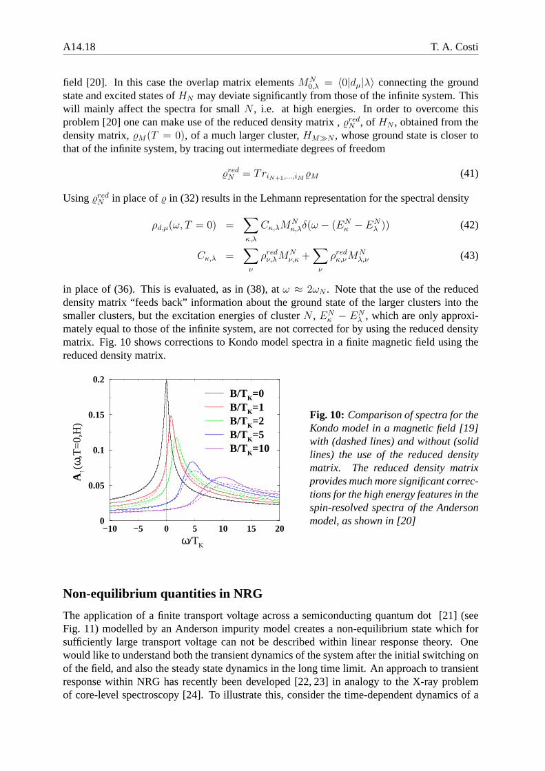
mately equal to those of the infinite system, are not corrected for by using the reduced densitymatrix. Fig. 10 shows corrections to Kondo model spectra in afinite magnetic field using thereduced density matrix.

−10 −5 0 5 10 15 20ω/TK

0

0.05

0.1

0.15

0.2

A↑(

ω,T

=0,

H)

B/TK=0B/TK=1B/TK=2B/TK=5B/TK=10

Fig. 10: Comparison of spectra for theKondo model in a magnetic field [19]with (dashed lines) and without (solidlines) the use of the reduced densitymatrix. The reduced density matrixprovides much more significant correc-tions for the high energy features in thespin-resolved spectra of the Andersonmodel, as shown in [20]

Non-equilibrium quantities in NRG

The application of a finite transport voltage across a semiconducting quantum dot [21] (seeFig. 11) modelled by an Anderson impurity model creates a non-equilibrium state which forsufficiently large transport voltage can not be described within linear response theory. Onewould like to understand both the transient dynamics of the system after the initial switching onof the field, and also the steady state dynamics in the long time limit. An approach to transientresponse within NRG has recently been developed [22, 23] in analogy to the X-ray problemof core-level spectroscopy [24]. To illustrate this, consider the time-dependent dynamics of a


DOT

2DEG

L

2DEG

V V V

V V

G R

RL

Fig. 11: Top view of a quantum dot.A confined region of electrons (the“quantum dot”) is formed out of thetwo dimensional electron gas (2DEG)at the interface of a GaAs/AlGaAs het-erostructure by patterning electrodesas shown and applying negative volt-ages. The constrictions at the left andright connect the dot electrons to theremaining 2DEG. Confinement impliesdistrict levels and large Coulomb re-pulsion on the dot, so this system be-haves like an Anderson impurity modelwith tunable hybridization matrix ele-ments (viaVL,R) and level position (viaVG).

Kondo spin subject to an initial state preparation att < 0and a sudden perturbation att = 0 ofthe form

H(t) = [1− θ(t)]HI + θ(t)HF (44)

We take the initial state Hamiltonian,HI , to be the anisotropic Kondo model with a local mag-netic field−BSz, B → ∞ forcing the spin to have〈Sz〉 = 1/2 for timest < 0 and the finalstate Hamiltonian,HF , to beHAKM with the local magnetic field switched off. An interestingquestion is whetherP (t) = 〈Sz(t)〉I , with I = e−βHI , exhibits coherent or incoherent dynam-ics. By obtaining the many-body eigenstates|mI〉 (|mF 〉) and eigenvaluesEmI

(EmF) of HI

(HF ) using the NRG, one can obtain the Fourier transform ofP (t) in Lehmann representation

P (ω) =∑

mI ,mF ,m′

F

e−βEmI

ZI

〈mI |mF 〉〈m′F |mI〉〈mF |Sz|m′

F 〉δ(ω − (EmF− Em′

F)) (45)

In contrast to equilibrium dynamical quantities (36), no ground state energy appears in theabove expression forP (ω) (even forT = 0), reflecting the absence of a ground state in a non-equilibrium situation. This also implies, that in evaluating (45), at a frequencyω = ωN wecannot simply use the excitations ofHF from a single clusterM = N . Instead excitationsbetween arbitrary excited states ofHF arising from all cluster sizes contribute and have to betaken into account [22]. The approximation of using a singleshellM = N to evaluate (45) atω = ωN ,

P (ωN) ≈∑

mF ,m′

F

〈mI,GS|mF 〉N〈m′F |mI,GS〉N〈mF |Sz|m′

F 〉Nδ(ω − (ENmF

− ENm′

F)) (46)

is valid for short time scales (t ≤ 1/TK) or high frequencies (ω ≫ TK). Typical results areshown in Fig. 12. Recently, the problem of summing over all energy shells proposed in [22] hasbeen solved [23]. In [23], a complete basis set of states for the Hilbert space ofHI,F is used,made up not from the retained states of theHN

I,F , but from the high energy states eliminatedat each stepN . Since, asN → ∞, all states are eliminated, the set of all eliminated statesisa complete eigenbasis ofHI,F . This allows contributions toP (ω) from all energy shells to besummed up, thereby allowing the study of the long-time behaviour of transient dynamics [23].

A14.20 T. A. Costi

10−2

10−1

100

101

102

tΩ0

−0.2

0.0

0.2

0.5

P(t

)Anisotropic KM (Ohmic TS model)

α=0.1

α=0.2

α=0.375

α=0.4

Fig. 12: P (t) = 〈Sz(t)〉 for the AKMobtained from Fourier transformingthe P (ω) [22] of (46) for severalρJ‖ corresponding to the dissipationstrengthsα = (1− 2

πtan−1(πρJ‖/4))

2

shown in the figure. The crossover toincoherent behaviour occurs atα =1/2. Ω0 is the unrenormalized fre-quency of tunneling oscillations atα =0.

NRG as a “quantum impurity solver” in DMFT

As described in the lecture of Liebsch in this book, it is possible, using dynamical mean fieldtheory (DMFT), to approximate models of correlated electrons on a lattice by a quantum impu-rity embedded in an effective medium (bath) which has to be determined self-consistently. Forexample, the Hubbard model can be mapped onto an effective Anderson impurity model with ahybridization function∆(ω), whose frequency dependence is unknown and needs to be deter-mined from the DMFT self-consistency condition. This requires the impurity Green functionGdσ to be identical to the local lattice Green functionG0σ =

∑

k 1/(ω+µ− εk −Σ(ω)), whereµ is the chemical potential,εk the dispersion relation of the lattice andΣ(ω) is the electronself-energy, identified as the impurity self-energy in DMFT. A highly accurate representation ofΣ(ω) for quantum impurity models has been introduced in [29] and finds application in DMFT.Fig. 13 shows the behaviour of theT = 0 spectra for the Hubbard model on going through themetal-insulator transition using this approach.

−8 −4 0 4 8ω

0.0

0.1

0.2

0.3

0

0.1

0.2

0.3

A(ω

)

0

0.1

0.2

0.3

0.4

−8 −4 0 4 8ω

0

0.1

0.2

0.3

0

0.1

0.2

0.3

0

0.1

0.2

0.3

0.4Bethe hypercubic

U=1.1Uc

U=0.99U

U=0.8U

c

cU=0.8U

U=0.99U

U=1.1Uc

c

c

Fig. 13: Local spectral density ofthe Hubbard model on Bethe andhypercubic lattices showing how theT = 0 metal-insulator transition oc-curs with increasing Coulomb interac-tion U [25]. For U < Uc the system ismetallic with a quasi-particle peak atω = 0, whereas forU > Uc the sys-tem is insulating with a gap betweenthe upper and lower Hubbard bands


6 Summary

The NRG transformation for the Kondo model is a powerful tool for the study of quantumimpurity models. It gives information on the many-body eigenvalues and eigenstates of suchmodels on all energy scales and thereby allows the direct calculation of their thermodynamic,dynamic, and transport properties. Recently it has been further developed to yield the transientresponse of these systems to sudden perturbations for both short and long-time limits [22,23].The method has been extended in new directions, such as to models with bosonic baths [26]to study spin-boson models and the interplay of correlations and phonon effects in Anderson-Holstein models [27]. It has also been used successfully to make progress on understandingthe Mott transition, heavy fermion behaviour and other phenomena in correlated lattice models[15,25,28].There is room for further improvement and extensions of the method both technically and inthe investigation of more complex systems such as multi-orbital models [30]. The use of a log-arithmic discretization of the conduction band, for example, gives rise to insufficient resolutionat higher energies. Approaches [17] for overcoming these difficulties are therefore of interest.The NRG also has potential to give information on the non-equilibrium transport through corre-lated impurity systems such as quantum dots. However, away from equilibrium, the absence ofa ground state requires new criteria other than energy for eliminating unimportant states. Ideasbased on the DMRG may prove useful in this respect.

Appendices

A Lanczos procedure

Neglecting spin indices, the conduction electron operatoris

Hc =∑

k

εkc+k ck

The Lanczos algorithm for tridiagonalizing this operator by repeated action on the state|0〉 is

|1〉 =1

λ0[Hc|0〉 − |0〉〈0|Hc|0〉] (47)

|n+ 1〉 =1

λn[Hc|n〉 − |n〉〈n|Hc|n〉 − |n− 1〉〈n− 1|Hc|n〉] (48)

yielding

Hc =∞∑

n=0

ǫnf+n fn + λn(f

+n fn+1 +H.c.) (49)

whereǫn = 〈n|Hc|n〉 andλn are normalizations obtained from (47-48).

A14.22 T. A. Costi

B Logarithmic discretization approximation

The approximation

Hc =

∫ +1

−1

dε ε c+ε,µcε,µ ≈∞∑

n=0

(ε−nc+−n,µc−n,µ + ε+nc

++n,µc+n,µ) (50)

used to replace the continuum band in (11) by the discrete onein (14) can be analyzed byintroducing a complete orthonormal basis set of states for the conduction electrons in eachinterval±[Λ−(n+1),Λ−n] using the following wavefunctions

ψ±np(ε) =

Λn/2

(1−Λ−1)1/2e±iωnpε for Λ−(n+1) < ±ε < Λ−n

0 otherwise(51)

Here p is a Fourier harmonic index andωn = 2πΛn/(1 − Λ−1). The operatorscεσ can beexpanded in terms of a complete set of new operatorsanpσ, bnpσ labeled by the intervaln andthe harmonic indexp

cεσ =∑

np

[anpσψ+np(ε) + bnpσψ

−np(ε)]. (52)

In terms of these operators, the Kondo Hamiltonian becomes,

HKM =1

2(1 + Λ−1)

∑

np

Λ−n(a†npσanpσ − b†npσbnpσ)

+(1− Λ−1)

2πi

∑

n

∑

p 6=p′

Λ−n(a†npσanp′σ − b†npσbnp′σ)e2πi(p−p′)

1−Λ−1

+ Jf+0,µ~σµνf0,ν .~S (53)

where in terms of the new operators,f0,µ = 1√2

∫ +1

−1dε cε,µ contains onlyp = 0 states:

f0,µ =1√2

∫ +1

−1

dε cε,µ =

[1

2(1− Λ−1)

]1/2 ∞∑

n=0

Λ−n/2(an0µ + bn0µ) (54)

We notice that only thep = 0 harmonic appears in the local Wannier state. This is a consequenceof the assumption that the Kondo exchange is independent ofk. Hence the conduction electronorbitalsanp, bnp for p 6= 0 only couple to the impurity spin indirectly via their coupling to thean0, bn0 in the second term of (53). This coupling is weak, being proportional to(1−Λ−1), andvanishes in the continuum limitΛ −→ 1, so these states may be expected to contribute littleto the impurity properties compared to thep = 0 states. This is indeed the case as shown byexplicit calculations in [1]. The logarithmic discretization approximation consists of neglectingconduction electron states withp 6= 0, resulting inHc given by Eq. (50) withc+n,µ ≡ an,0,µ andc−n,µ ≡ bn,0,µ and a discrete Kondo Hamiltonian given by Eq. (14).


References

[1] K. G. Wilson, Rev. Mod. Phys.47, 773 (1975)

[2] P. Nozieres, J. Low Temp. Phys.17, 31 (1974)

[3] A. C. Hewson,The Kondo Problem to Heavy Fermions, Cambridge University Press(1993)

[4] P. W. Anderson, J. Phys. C3, 2439 (1970)

[5] U. Weiss,Quantum Dissipative Systems, Series in Modern Condensed Matter Physics,Vol. 2, 2nd edition, World Scientific, Singapore (1999); A. J. Leggett, S. Chakravarty, A.T. Dorsey, M. P. A. Fisher, A. Garg and W. Zwerger, Rev. Mod. Phys.59,1 (1987)

[6] W. J. de Haas, J. de Boer and G. J. van den Berg, Physica1, 1115 (1934).

[7] P. W. Anderson, Phys. Rev.124, 41 (1961)

[8] R. Bulla, Th. Pruschke and A. C. Hewson, J. Phys. Cond. Matt.9, 10463 (1997)

[9] H. B. Krishnamurthy, J. W. Wilkins and K. G. Wilson, Phys. Rev. B 21, 1044 (1980)

[10] S. R. White, Phys. Rev. Lett.69, 2863 (1992); Phys. Rev. B48, 10345 (1993); Phys. Rep.301, 187 (1998); S. R. White and R. M. Noack, Phys. Rev. Lett.68, 3487 (1992)

[11] K. G. Wilson and J. Kogut, Phys. Rep. C12, 75 (1974)

[12] T. A. Costi and C. Kieffer, Phys. Rev. Lett.76, 1683 (1996); T. A. Costi, Phys. Rev. Lett.80, 1038 (1998); T. A. Costi and G. Zarand, Phys. Rev. B59, 12398 (1999)

[13] O. Sakai, Y. Shimizu and T. Kasuya, J. Phys. Soc. Jap.583666 (1989)

[14] T. A. Costi and A. C. Hewson, Phil. Mag. B65, 1165 (1992); T. A. Costi, A. C. Hewsonand V. Zlatic J. Phys. Condens. Matt.6, 2519 (1994)

[15] R. Bulla, T. A. Costi and D. Vollhardt, Phys. Rev. B64, 045103 (2001)

[16] W. Metzner and D. Vollhardt, Phys. Rev. Lett.62, 324 (1989); A. Georges, G. Kotliar, W.Krauth and M. J. Rozenberg, Rev. Mod. Phys.68, 13 (1996)

[17] M. Yoshida, M. A. Whitaker and L. N. Oliveira, Phys. Rev. B41, 9403 (1990)

[18] W. C. Oliveira and L. N. Oliveira, Phys. Rev. B49, 11992 (1994); S. C. Costa, C. A. Paula,V. L. L ıbero and L. N. Oliveira, Phys. Rev. B55, 30 (1997)

[19] T. A. Costi, Phys. Rev. Lett.85, 1504 (2000); Phys. Rev. B64, 241310 (2001)

[20] W. Hofstetter, Phys. Rev. Lett.85, 1508 (2000)

[21] D. Goldhaber-Gordon, J. Gores, M. A. Kastner, H. Shtrikman, D. Mahalu and U. Meirav,Phys. Rev. Lett.81, 5225 (1998)

[22] T. A. Costi, Phys. Rev. B55, 3003 (1997)

A14.24 T. A. Costi

[23] F. Anders and A. Schiller, Phys. Rev. Lett.95, 196801 (2005)

[24] P. Nozieres and C. T. De Domenicis,Phys. Rev.178, 1097 (1969).

[25] R. Bulla, Phys. Rev. Lett.83, 136 (1999)

[26] R. Bulla, H-Y. Lee, N-H. Tong and M. Vojta, Rev. B71, 045122 (2005)

[27] A. C. Hewson, D. Meyer, J. Phys. Condens. Matter14, 427 (2002).

[28] T. Pruschke, R. Bulla and M. Jarrell, Phys. Rev. B61, 12808 (1999); T. A. Costi and N.Manini, J. Low Temp. Phys.126, 835 (2002)

[29] R. Bulla and Th. Pruschke and A. C. Hewson, J. Phys. Cond. Matt. 10, 8365 (1998)

[30] T. Pruschke and R. Bulla, European Physical Journal B44, 217 (2005)

nrg lecture - scientific it systems

Documents