objective detection of oceanic eddies and the agulhas...

Objective Detection of Oceanic Eddies and the Agulhas Leakage

FRANCISCO J. BERON-VERA, YAN WANG, AND MARIA J. OLASCOAGA

Rosenstiel School of Marine and Atmospheric Science, University of Miami, Miami, Florida

GUSTAVO J. GONI

National Oceanic and Atmospheric Administration/Atlantic Oceanographic and Meteorological Laboratory, Miami, Florida

GEORGE HALLER

Institute for Mechanical Systems, ETH Z€urich, Zurich, Switzerland

(Manuscript received 13 September 2012, in final form 14 March 2013)

ABSTRACT

Mesoscale oceanic eddies are routinely detected from instantaneous velocities derived from satellite al-

timetry data. While simple to implement, this approach often gives spurious results and hides true material

transport. Here it is shown how geodesic transport theory, a recently developed technique from nonlinear

dynamical systems, uncovers eddies objectively. Applying this theory to altimetry-derived velocities in the

South Atlantic reveals, for the first time, Agulhas rings that preserve their material coherence for several

months, while ring candidates yielded by other approaches tend to disperse or leak within weeks. These

findings suggest that available velocity-based estimates for the Agulhas leakage, as well as for its impact on

ocean circulation and climate, need revision.

1. Introduction

Oceanic eddies are commonly envisaged as whirling

bodies of water that preserve their shape, carrying mass,

momentum, energy, thermodynamic properties, and bio-

geochemical tracers over long distances (e.g., Robinson

1983). While this widespread view on eddies is funda-

mentally Lagrangian (material), most available eddy

detection methods are Eulerian (velocity based).

Eulerian detection of mesoscale eddies (with di-

ameters ranging from 50 to 250 km) is routinely applied

to instantaneous velocities derived from satellite altim-

etry measurements of sea surface height (SSH). In some

cases, eddies are identified from the Okubo–Weiss cri-

terion as regions where vorticity dominates over strain

(e.g., Chelton et al. 2007; Henson and Thomas 2008;

Isern-Fontanet et al. 2003; Morrow et al. 2004). In other

cases, eddies are sought as regions filled with closed

streamlines of the SSH field (e.g., Chelton et al. 2011a,b;

Fang and Morrow 2003; Goni and Johns 2001) or as

features obtained from a wavelet-packet decomposition

of the SSH field (Doglioli et al. 2007; Turiel et al. 2007).

These detection methods invariably use instantaneous

Eulerian information to reach long-term conclusions

about fluid transport. Furthermore, they give different

results in reference frames that move or rotate relative

to each other.

The problem with the use of instantaneous velocities

is their inability to reveal long-range material transport

and coherence in unsteady flows (Batchelor 1964). An

example is shown in Fig. 1, where the instantaneous

velocity field is classified as eddy-like for all times by

each of the Eulerian criteria mentioned above. Specifi-

cally, vorticity dominates over strain, and streamlines

are closed for all times. Yet actual particle motion turns

out to be governed by a rotating saddle point with no

closed transport barriers (Haller 2005).

Figure 1 also highlights the issue with frame-dependent

eddy detection, whether Eulerian or Lagrangian. Truly

unsteadyflowshavenodistinguished reference frames: such

flows remain unsteady in any frame (Lugt 1979). Conclu-

sions about flow structures, therefore, should not depend

on the chosen frame, because it is not a priori known

which—if any—frame reveals those structures correctly.

Corresponding author address: F. J. Beron-Vera, RSMAS/AMP,

University of Miami, 4600 Rickenbacker Cswy., Miami, FL 33149.

E-mail: [email protected]

1426 JOURNAL OF PHYS ICAL OCEANOGRAPHY VOLUME 43

DOI: 10.1175/JPO-D-12-0171.1

� 2013 American Meteorological Society

Beyond conceptual problems, Eulerian eddy detection

yields noisy results, necessitating the use of filtering and

threshold parameters. Applying such detection methods

to altimetry data, Souza et al. (2011) report variabilities

up to 50% in the number of eddies detected, depending

on the choice of parameters and filtering methods. A

systematic comparison of these varying numbers with

actual material transport is difficult because of the

sparseness of in situ hydrographic measurements and

Lagrangian data. In particular, most useful drifter tra-

jectory data are only available from dedicated experi-

ments, and satellite ocean color imagery is constrained

by cloud cover or the absence of biological activity. This

in turn implies that Eulerian predictions for Lagrangian

eddy transport have remained largely unverified.

These shortcomings of contemporary eddy detection

are important to consider when quantifying transport by

eddies. For instance, recent studies suggest that long-range

transport by anticyclonic mesoscale eddies (Agulhas

rings) pinched off from the Agulhas Current retroflec-

tion is a potential moderating factor in global climate

change. Known as the largest eddies in the ocean (Olson

and Evans 1986), Agulhas rings transport warm and

salty water from the Indian Ocean into the South At-

lantic (Agulhas leakage). They may also possibly reach

the upper arm of the Atlantic meridional overturning

circulation (AMOC) when driven northwestward by

the Benguela Current and its extension (Gordon 1986).

Following an apparent southward shift in the subtropical

front (Ridgway and Dunn 2007), the intensity of the

Agulhas leakage has been on the rise (Biastoch et al.

2009), leading to speculation that it may counteract the

slowdown of theAMOCbecause ofArctic icemelting in

a warming climate (Beal et al. 2011). To assess this con-

jecture, an accurate Lagrangian identification of Agulhas

rings is critical.

Indeed, most eddies identified from Eulerian foot-

prints will disperse over relatively short times. While

some of these dispersing features still drag water in their

wakes, the transported water will stretch and fold be-

cause of the lack of a surrounding, coherent material

boundary. As a consequence, distinguished features of

the transported water, such as high temperature and

salinity, will be quickly lost because of enhanced diffu-

sion across filamented material boundaries.

Counteracting the effects of melting Arctic ice on

AMOC requires a supply of warm and salty water (Beal

et al. 2011). Agulhas rings with persistent and coherent

material cores deliver this type of water directly from its

source, the Agulhas leakage. By contrast, transient Eu-

lerian ring-like features mostly stir the ocean without

creating the clear northwest pathway for temperature

and salinity envisioned by Gordon (1986).

In steady flow, coherent material eddies are readily

identified as regions of closed streamlines. In near-steady

flows with periodic time dependence, the Kolmogorov–

Arnold–Moser (KAM) theory (cf., e.g., Arnold et al.

2006) reveals families of nested closed material curves

(so-called KAM curves) that assume the same position

in the flow after each temporal period. An outermost

such KAM curve from a given family, therefore, plays

the role of a coherent material eddy boundary. This

result extends to near-steady time-quasiperiodic flows,

in which KAM curves are quasiperiodically deforming

closed material lines (Jorba and Sim�o 1996).

Identifying similar material boundaries for coherent

eddies in general unsteady flows has been an open prob-

lem. Recently, however, Haller and Beron-Vera (2012)

developed a new mathematical theory of transport bar-

riers that, among other features, identifies generalized

KAM curves (elliptic transport barriers) for arbitrary

unsteady flows. Here we use this new theory to devise a

methodology, geodesic eddy detection, for the objective

identification ofLagrangian eddy boundaries in the ocean.

Analyzing altimetry measurements in the eastern

side of the South Atlantic subtropical gyre, we find that

geodesic eddy detection significantly outperforms avail-

able Eulerian and Lagrangian methods in locating long-

lived and coherentAgulhas rings.An independent analysis

of available satellite ocean color (chlorophyll) data cor-

roborates our results by showing localized and persistent

biological activity in an eddy identified using geodesic

eddy detection. Our findings suggest that Eulerian esti-

mates of the volume of water transported byAgulhas rings

in a coherent manner are significantly exaggerated.

Geodesic eddy detection is outlined in section 2, which

is organized into four subsections. Section 2a presents the

dynamical systems setup for studying material transport.

The rationale behind the geodesic transport theory of

Haller and Beron-Vera (2012) is reviewed in section 2b.

Section 2c covers the notion of shear transport barriers.

The definition of coherent material eddy boundary is

given in section 2d. Our main results are presented in

section 3. The conclusions are stated in section 4. Ap-

pendix A describes the velocity data on which geodesic

FIG. 1. A planar unsteady velocity field identified as an eddy by

Eulerian criteria. In an appropriate rotating frame, however, the

velocity field becomes a steady saddle flowwith no closed transport

barriers.

JULY 2013 BERON -VERA ET AL . 1427

eddy detection is applied. The algorithmic steps of

geodesic eddy detection are summarized in appendix B.

Finally, computational details are given in appendix C.

2. Geodesic eddy detection

a. Dynamical systems setup

Consider an unsteady flow on the plane with velocity

field v(x, t), where x 5 (x, y) denotes position and t is

time. The evolution of fluid particle positions in this flow

satisfies a nonautonomous dynamical system given by

the following differential equation:

dx

dt5 v(x, t) . (1)

Material transport in (1) is determined by the properties

of the flow map,

Ftt0: x01 x(t; x0, t0) , (2)

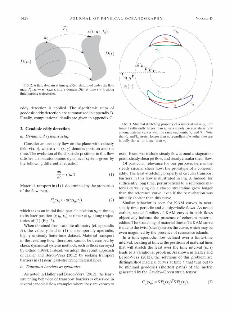
which takes an initial fluid particle position x0 at time t0to its later position (t; t0, x0) at time t 6¼ t0, along trajec-

tories of (1) (Fig. 2).

When obtained from satellite altimetry (cf. appendix

A), the velocity field in (1) is a temporally aperiodic,

highly unsteady finite-time dataset. Material transport

in the resulting flow, therefore, cannot be described by

classic dynamical systemsmethods, such as those surveyed

by Ottino (1989). Instead, we adopt the recent approach

of Haller and Beron-Vera (2012) by seeking transport

barriers in (1) near least-stretching material lines.

b. Transport barriers as geodesics

As noted in Haller and Beron-Vera (2012), the least-

stretching behavior of transport barriers is observed in

several canonical flow examples where they are known to

exist. Examples include steady flow around a stagnation

point, steady shear jet flow, and steady circular shear flow.

Of particular relevance for our purposes here is the

steady circular shear flow, the prototype of a coherent

eddy. The least-stretching property of circular transport

barriers in this flow is illustrated in Fig. 3. Indeed, for

sufficiently long time, perturbations to a reference ma-

terial curve lying on a closed streamline grow longer

than the reference curve, even if the perturbation was

initially shorter than this curve.

Similar behavior is seen for KAM curves in near-

steady time-periodic and quasiperiodic flows. As noted

earlier, nested families of KAM curves in such flows

objectively indicate the presence of coherent material

eddies. The stretching of material lines off a KAM curve

is due to the twist (shear) across the curve, which may be

even magnified by the presence of resonance islands.

In a time-aperiodic flow defined over a finite-time

interval, locating at time t0 the positions of material lines

that will stretch the least over the time interval (t0, t)

leads to a variational problem. As shown in Haller and

Beron-Vera (2012), the solutions of this problem are

distinguished material curves at time t0 that turn out to

be minimal geodesics (shortest paths) of the metric

generated by the Cauchy–Green strain tensor,

Ctt0(x0)5$Ft

t0(x0)

T$Ftt0(x0) , (3)

FIG. 2. A fluid domain at time t0,D(t0), deformed under the flow

map, Ftt0: x0 1 x(t; x0, t0), into a domain D(t) at time t 6¼ t0 along

fluid particle trajectories.

FIG. 3. Minimal stretching property of a material curve gt0 , for

times t sufficiently larger than t0, in a steady circular shear flow

among material curves with the same endpoints, gt0 and gt0 . Note

that gt0 and gt0 stretch longer than gt, regardless of whether they are

initially shorter or longer than gt0 .


where superscript T denotes transpose and $ refers to

the spatial gradient operator.

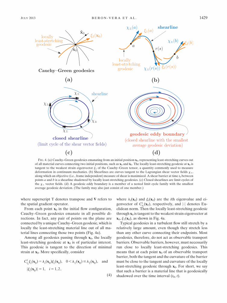
From each point x0 in the initial flow configuration,

Cauchy–Green geodesics emanate in all possible di-

rections. In fact, any pair of points on the plane are

connected by a unique Cauchy–Green geodesic, which is

locally the least-stretching material line out of all ma-

terial lines connecting those two points (Fig. 4a).

Among all geodesics passing through x0, the locally

least-stretching geodesic at x0 is of particular interest.

This geodesic is tangent to the direction of minimal

strain at x0. More specifically, consider

Ctt0ji(x0)5 li(x0)ji(x0), 0, l1(x0)# l2(x0), and

jji(x0)j5 1, i5 1, 2,

(4)

where li(x0) and ji(x0) are the ith eigenvalue and ei-

genvector of Ctt0(x0), respectively, and j�j denotes Eu-

clidean norm. Then the locally least-stretching geodesic

through x0 is tangent to the weakest strain eigenvector at

x0, j1(x0), as shown in Fig. 4a.

Typical geodesics in a turbulent flow still stretch by a

relatively large amount, even though they stretch less

than any other curve connecting their endpoints. Most

geodesics, therefore, do not act as observable transport

barriers. Observable barriers, however, must necessarily

run close to locally least-stretching geodesics. This

means that at each point x0 of an observable transport

barrier, both the tangent and the curvature of the barrier

must be close to the tangent and curvature of the locally

least-stretching geodesic through x0. For short, we say

that such a barrier is a material line that is geodesically

shadowed over the time interval (t0, t).

FIG. 4. (a) Cauchy–Green geodesics emanating from an initial position x0, representing least-stretching curves out

of all material curves connecting two initial positions, such as x0 and x0. The locally least-stretching geodesic at x0 istangent to the weakest strain eigenvector j1 of the Cauchy–Green tensor, a quantity commonly used to measure

deformation in continuum mechanics. (b) Shearlines are curves tangent to the Lagrangian shear vector fields x6,

along which an objective (i.e., frame independent) measure of shear is maximized. A shear barrier at time t0 between

points a and b is a shearline shadowed by locally least-stretching geodesics. (c) Closed shearlines are limit cycles of

the x6 vector fields. (d) A geodesic eddy boundary is a member of a nested limit cycle family with the smallest

average geodesic deviation. (The family may also just consist of one member.)


c. Shear barriers

With the behavior of streamlines in the steady circular

flow example in mind, it is natural to seek the transport

barriers of interest as those maximizing shear. An ap-

propriate frame-independent form of shear in unsteady

flows is given by the Lagrangian shear, defined as the

tangential projection of the linearly advected normal to

a material line. As shown in Haller and Beron-Vera

(2012), Lagrangian-shear-maximizing transport barriers

(or shear barriers) over (t0, t) turn out to be geodesically

shadowed trajectories of the Lagrangian shear vector

fields

x6(x0)5a1(x0)j1(x0)6a2(x0)j2(x0),

ai(x0)5

ffiffiffiffiffiffiffiffiffiffiffiffiffiffiffiffiffiffiffiffiffiffiffiffiffiffiffiffiffiffiffiffiffiffiffiffiffiffiffiffiffiffiffiffiffiffiffiffiffiffiffiffiffiffilj(x0)

qffiffiffiffiffiffiffiffiffiffiffiffiffil1(x0)

p1

ffiffiffiffiffiffiffiffiffiffiffiffiffil2(x0)

pvuut

, i 6¼ j . (5)

Closeness of a trajectory (or shearline) of (5) to its

shadowing least-stretching geodesic at x0 can be com-

puted as the sum of their tangent and curvature differ-

ences. This sum, the geodesic deviation of a shearline,

can be proven to be equal to (Haller and Beron-Vera

2012)

dx6g (x0)5 j12a1j1

��a11

l1l2

2 1

�k1 7 a2k2

7$a1 � x6

a2

2$l1 � j22l2

�� , (6)

where

ki(x0)5$ji(x0)ji(x0) � jj(x0), i 6¼ j (7)

is the curvature of the curve tangent to the ith strain

eigenvector field at x0 (Fig. 4b).

Shear barriers are either open curves (parabolic bar-

riers) or closed curves (elliptic barriers). While sets of

parabolic barriers generalize the concept of a shear jet to

arbitrary unsteady flow, elliptic barriers generalize the

concept of a KAM curve. As limit cycles of the shear

vector field (Fig. 4c), elliptic barriers are robust with

respect to perturbations of the underlying velocity data,

and hence smoothly persist under moderate noise and

small changes to the observational time interval (t0, t).

d. Eddy boundaries

If elliptic barriers occur in a nested family, the out-

ermost barrier is the physically observed eddy boundary,

enclosing the largest possible coherent water mass in the

region. Outermost elliptic barriers, however, also tend

to be themost sensitive to errors and uncertainties in the

velocity data.

To obtain a robust eddy boundary, we select the

member of a nested family of closed shearlines which

has the lowest average geodesic deviation, hdx6g i, in the

family (Fig. 4d). As discussed in Haller and Beron-Vera

(2012), hdx6g i along an elliptic barriermeasures howmuch

the barrier extraction procedure has converged over the

time interval (t0, t). Accordingly, an elliptic barrier with

the lowest hdx6g i value in a nested family of barriers is the

best eddy barrier candidate. As such, it is also the least

susceptible to errors and uncertainties. Based on these

considerations, geodesic eddy detection comprises the

algorithmic steps described in appendix B.

We finally note that, in incompressible flows, elliptic

barriers have two important conservation properties: 1)

they preserve the area they enclose and 2) they reassume

their initial arclength at time t (Fig. 5) (Haller and

Beron-Vera 2012). These two properties make elliptic

barriers ideal boundaries for coherent eddy cores.

3. Results

We consider a region of the South Atlantic subtropical

gyre, bounded by longitudes (148W, 98E) and latitudes

(398S, 218S), which encompasses possible routes of

Agulhas rings (dashed rectangle in each panel of Figs. 7

and 9). The same region has been analyzed byBeron-Vera

et al. (2008), who showed that the finite-time Lyapunov

exponent, a widely used Lagrangian diagnostic (Haller

2001; Peacock and Dabiri 2010), does not reveal coherent

material eddies. More recently, the same area was also

studied by Lehahn et al. (2011), who reported observa-

tions of a nearly isolated mesoscale chlorophyll patch,

FIG. 5. Schematics of a closed shearline gt0 computed using flow

data over the time interval (t0, t). The dashed curve indicates

a translated and rotated position of gt0 for reference. If the flow is

incompressible, the advected material line gt has the same ar-

clength, and encloses the same area, as gt0 .


traversing the region in the period from November 2006

to September 2007.

We apply geodesic eddy detection to altimetry-derived

currents (cf. appendix A) in the selected region starting

on t05 24 November 2006, with the detection time scale

set to T 5 t 2 t0 5 90 days. Following the algorithmic

steps described in appendix B, with numerical details

given in appendix C, geodesic eddy detection isolates

two coherent material eddies (denoted geodesic eddies).

The boundary of the first eddy is obtained as a limit cycle

of the x1(x0) shear vector field, with an anticyclonic

polarity. The boundary of the second eddy is recovered

as a limit cycle of the x2(x0) field, with a cyclonic po-

larity. The extraction of the anticyclonic eddy boundary

is detailed in Fig. 6. The geographical locations of the

two eddies identified on 24 November 2006 are shown in

the upper-left panel of Fig. 7, with the anticyclonic eddy

indicated in red and the cyclonic eddy in blue.

The remaining panels in the left column of Fig. 7 show

several later advected positions of the two geodesic

eddies to illustrate their coherence. Note the complete

lack of material filamentation or leakage from these

eddies over 90 days. This can be seen in more detail in

the right column of Fig. 8, which shows the two eddies on

the detection date and 90 days later. Closed material

lines like the boundaries of these eddies are highly

atypical in an otherwise turbulent flow. Their role is

indeed best compared to the role of KAM curves in

time-periodic or quasiperiodic flows.

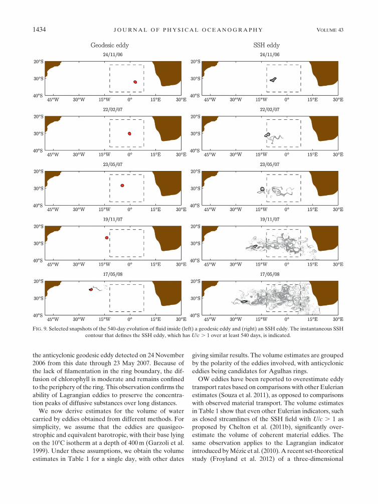
Remarkably, the coherence of the anticyclonic eddy is

preserved well over the 90-day period on which our

computations were performed (Fig. 9, left column). In-

deed, this eddy preserves its coherence even 540 days

later, exhibiting only translation, rotation, and minor

deformation without noticeable leakage, stretching or

folding. The remarkable coherence of this eddy can at-

tributed to its interior being foliated by a large number

of nested closed shearlines. The inner shearlines are less

exposed to the ambient turbulent mixing than the outer

ones, thereby providing a stability buffer for the eddy.

By contrast, the boundary of the cyclonic eddy is the

only member of a family of nested closed shearlines.

With the stability buffer absent, the boundary of this

eddy exhibits filamentation immediately after 90 days.

For comparison, the remaining columns of Fig. 7 il-

lustrate the accuracy of the two most widely used Eu-

lerian eddy diagnostics and one recent Lagrangian eddy

diagnostic on the same dataset.

The middle-left column of Fig. 7 shows the material

evolution of eddies (denoted SSH eddies) obtained from

the method of Chelton et al. (2011b), who argue that

closed SSH contours can play roughly the same role in

inhibiting transport as closed streamlines do in steady

flows. Chelton et al. (2011b) suggest that this should be

the case when the rotational speed of the eddy U dom-

inates its translational speed, c (cf. also Early et al. 2011).

More specifically, Chelton et al. (2011b) propose that

U/c. 1 should signal the presence of a coherent eddy, as

opposed to a linear wave (U/c , 1). However, as re-

vealed by the Lagrangian evolution of closed SSH con-

tours in the upper-middle row of Fig. 7 (all with U/c. 1

over at least 90 days), most such contours rapidly stretch

and fold, exhibiting leakage and filamentation that dis-

qualifies them as physically reasonable coherent

FIG. 6. Identification of a coherent material eddy boundary on

t0 5 24 November 2006 from geodesic eddy detection with de-

tection time scale T 5 t 2 t0 5 90 days. Marked in red, the eddy

boundary is obtained as an average-geodesic-deviation-minimizing

member of a nested family of limit cycles of the Lagrangian shear

vector field x1. (top) The full limit cycle family is shown in blue,

with gray arrows indicating the x1 vector field. (middle) The first

return (Poincar�e) map, x 1 P(x), onto a section S locally trans-

verse to x1 vector field is shown. Dots indicate the fixed points of

the Poincar�e map, P(x) 5 x, corresponding to each of the limit

cycles. (bottom) The distribution of the average geodesic deviation

over the limit cycles is shown.


FIG.7.(left)Selectedsnap

shotsofthe90-dayevolutionoffluid

insideeddiesidentifiedbygeodesiceddydetection;(middleleft)themethodofCheltonetal.(2011a)withU/c.

1overat

least90days;(m

iddle

right)theOkubo–Weiss(O

W)criterion;and(right)thecriterionofM� ezic

etal.(2010).


material eddy boundaries. Only two SSH eddies ap-

proximate coherent geodesic eddies on 24 November

2006 (Fig. 8, middle-left column). However, both eddies

exhibit almost instantaneous material filamentation

beyond that date. The panels in the right column of Fig.

9 further demonstrate the inability of an SSH eddy with

U/c. 1 for a period of at least 540 days to trap and carry

within water in a coherentmanner.We conclude that the

SSH contour approach, with or without the U/c . 1 re-

quirement, shows major inaccuracies in detecting mate-

rial eddies, including the overestimation of coherent

material eddy cores, as well as the generation of a large

number of false positives.1

The middle-right column of Fig. 7 documents similar

findings for the Okubo–Weiss criterion (Okubo 1970;

Weiss 1991), the other broadly used frame-dependent

Eulerian method for eddy identification. Relative to a

reference frame, this method identifies eddies (denoted

OW eddies) as regions of fluid where vorticity dominates

over strain. The regions indicated in black qualify as OW

eddies in the earth’s frame on 24 November 2006. In

a similar manner to SSH eddies, coherent geodesic

eddies on 24 November 2006 are roughly approximated

by two OW eddies, which deform rapidly after that date

(Fig. 8, middle-right column). The remainingOWeddies

are false positives for Lagrangian eddies: they undergo

intense stretching and filamentation, before fully dis-

persing a few months later. We conclude that when used

for coherent material eddy detection, the Okubo–Weiss

approach also shows major inaccuracies. This includes

the inability to capture actual coherent eddies accurately,

as well as well as the tendency to generate numerous false

positives. False negatives also arise once threshold values

(not discussed) are introduced for the Okubo–Weiss

parameter.

We now proceed to consider the application of the

more recent Lagrangian eddy diagnostic of M�ezic et al.

(2010). This approach views an incompressible flow re-

gion at time t0 as a mesoelliptic region if the eigenvalues

of the deformation gradient $Ftt0(x0) are complex for all

x0 in that region. Even though this approach is La-

grangian, the eigenvalues of $Ftt0(x0) are frame de-

pendent, and hence the resulting eddy candidates are

not objective. As noted in M�ezic et al. (2010), meso-

elliptic regions approach Okubo–Weiss elliptic regions

as t tends to t0. For increasing T 5 t 2 t0, mesoelliptic

regions (denoted ME eddies) tend to rapidly fill the full

domain of extraction, as most initial conditions accu-

mulate enough rotation in their evolution to create

complex eigenvalues for $Ftt0(x0). As a result, identify-

ing ME eddies over time scales longer than a few days

becomes unrealistic. Instead, we have chosen to use T54 days, following M�ezic et al. (2010).

Shown in the right colum of Fig. 7,ME eddies resemble

OW eddies closely, as expected. In a fashion similar to

OW eddies, only two ME eddies approximate the geo-

desic eddies detected on 24 November 2006. Just as OW

eddies, these ME eddies develop substantial material

filamentation beyond that date (Fig. 8, right column).

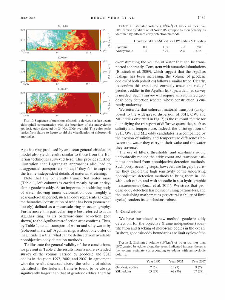
Independent observational evidence for the Lagrang-

ian eddies can be inferred from surface ocean chlorophyll

concentration in the South Atlantic. Figure 10 shows

a sequence of snapshots of chlorophyll concentration

derived from the Moderate Resolution Imaging Spec-

troradiometer (MODIS) sensor aboard the Aqua satel-

lite. Note the patch of high chlorophyll concentration,

discussed in Lehahn et al. (2011), which translates inside

FIG. 8. Fluid positions of eddy candidates obtained from different detection methods on t05 24 Nov 2006 and 90 days later. (middle left,

middle right, and right columns) The red and blue eddy candidates by other eddy detection methods are the closest ones to (left) the

similarly colored geodesic eddies.

1 Indeed, U/c / ‘ in the flow defined in Fig. 1.


the anticyclonic geodesic eddy detected on 24 November

2006 from this date through 23 May 2007. Because of

the lack of filamentation in the ring boundary, the dif-

fusion of chlorophyll is moderate and remains confined

to the periphery of the ring. This observation confirms the

ability of Lagrangian eddies to preserve the concentra-

tion peaks of diffusive substances over long distances.

We now derive estimates for the volume of water

carried by eddies obtained from different methods. For

simplicity, we assume that the eddies are quasigeo-

strophic and equivalent barotropic, with their base lying

on the 108C isotherm at a depth of 400m (Garzoli et al.

1999). Under these assumptions, we obtain the volume

estimates in Table 1 for a single day, with other dates

giving similar results. The volume estimates are grouped

by the polarity of the eddies involved, with anticyclonic

eddies being candidates for Agulhas rings.

OW eddies have been reported to overestimate eddy

transport rates based on comparisons with other Eulerian

estimates (Souza et al. 2011), as opposed to comparisons

with observed material transport. The volume estimates

in Table 1 show that even other Eulerian indicators, such

as closed streamlines of the SSH field with U/c . 1 as

proposed by Chelton et al. (2011b), significantly over-

estimate the volume of coherent material eddies. The

same observation applies to the Lagrangian indicator

introduced byM�ezic et al. (2010).A recent set-theoretical

study (Froyland et al. 2012) of a three-dimensional

FIG. 9. Selected snapshots of the 540-day evolution of fluid inside (left) a geodesic eddy and (right) an SSH eddy. The instantaneous SSH

contour that defines the SSH eddy, which has U/c . 1 over at least 540 days, is indicated.


Agulhas ring produced by an ocean general circulation

model also yields results similar to those from the Eu-

lerian techniques surveyed here. This provides further

illustration that Lagrangian approaches also lead to

exaggerated transport estimates, if they fail to capture

the frame-independent details of material stretching.

Note that the coherently transported water mass

(Table 1, left column) is carried mostly by an anticy-

clonic geodesic eddy. As an impermeable whirling body

of water showing minor deformation over roughly a

year-and-a-half period, such an eddy represents an exact

mathematical construction of what has been (somewhat

loosely) defined as a mesoscale ring in oceanography.

Furthermore, this particular ring is best referred to as an

Agulhas ring, as its backward-time advection (not

shown) to theAgulhas retroflection area confirms. Thus,

by Table 1, actual transport of warm and salty water by

(coherent material) Agulhas rings is about one order of

magnitude less than what can be deduced from available

nonobjective eddy detection methods.

To illustrate the general validity of these conclusions,

we present in Table 2 the results from a more extended

survey of the volume carried by geodesic and SSH

eddies in the years 1997, 2002, and 2007. In agreement

with the results discussed above, the volume of eddies

identified in the Eulerian frame is found to be always

significantly larger than that of geodesic eddies, thereby

overestimating the volume of water that can be trans-

ported coherently. Consistent with numerical simulations

(Biastoch et al. 2009), which suggest that the Agulhas

leakage has been increasing, the volume of geodesic

eddies (of both polarities) follows a similar trend. Clearly,

to confirm this trend and correctly assess the role of

geodesic eddies in the Agulhas leakage, a detailed survey

is needed. Such a survey will require an automated geo-

desic eddy detection scheme, whose construction is cur-

rently underway.

We reiterate that coherent material transport (as op-

posed to the widespread dispersion of SSH, OW, and

ME eddies observed in Fig. 7) is the relevant metric for

quantifying the transport of diffusive quantities, such as

salinity and temperature. Indeed, the disintegration of

SSH, OW, and ME eddy candidates is accompanied by

the erosion of salinity and temperature differences be-

tween the water they carry in their wake and the water

they traverse.

The use of filters, thresholds, and size-limits would

undoubtedly reduce the eddy count and transport esti-

mates obtained from nonobjective detection methods.

Such postprocessing steps, however, are largely heuris-

tic: they exploit the high sensitivity of the underlying

nonobjective detection methods to bring them in line

with each other, and with sporadic in situ hydrographic

measurements (Souza et al. 2011). We stress that geo-

desic eddy detection has no such tuning parameters, and

the underlying mathematics (structural stability of limit

cycles) renders its conclusions robust.

4. Conclusions

We have introduced a new method, geodesic eddy

detection, for the objective (frame independent) iden-

tification and tracking of mesoscale eddies in the ocean.

In short, geodesic eddy boundaries are limit cycles of the

TABLE 1. Estimated volume (104 km3) of water warmer than

108C carried by eddies on 24Nov 2006, grouped by their polarity, as

identified by different eddy detection methods.

Geodesic eddies SSH eddies OW eddies ME eddies

Cyclonic 0.5 11.5 19.2 19.8

Anticyclonic 1.0 23.5 35.4 37.2

TABLE 2. Estimated volume (104 km3) of water warmer than

108C carried by eddies along the years. Indicated in parentheses is

the volume estimate corresponding to eddies with anticyclonic

polarity.

Year 1997 Year 2002 Year 2007

Geodesic eddies 7 (5) 10 (9) 9 (7)

SSH eddies 63 (29) 62 (36) 57 (27)

FIG. 10. Sequence of snapshots of satellite-derived surface ocean

chlorophyll concentration with the boundary of the anticyclonic

geodesic eddy detected on 24 Nov 2006 overlaid. The color scale

varies from figure to figure to aid the visualization of chlorophyll

anomalies.


Lagrangian shear vector field that are the closest to least-

stretching geodesics of the Cauchy–Green strain tensor.

When tracked as material lines, geodesic eddy boundaries

in a two-dimensional incompressible flow preserve their

enclosed area and arclength, acting as impenetrable is-

lands of minimal deformation in an otherwise turbulent

flow. This in turn enables them to preserve the concen-

tration of diffusive tracers they carry for extended periods.

By the structural stability of limit cycles, geodesic eddy

boundaries are robust with respect velocity measure-

ment errors and changes in their detection period.

Using geodesic eddy detection, we have isolated highly

coherent Agulhas rings that carry warm and salty water

over large distances. Remarkably, one geodesic eddy

constructed from three months of data was found to

show no sign of disintegration up to one year and a half.

By comparison, eddies identified by two currently used

Eulerian methods and one recent Lagrangian diagnostic

showed clear signs of leakage and stretchingwithinweeks.

The volume of water that such eddies would transport if

they were coherent was found to be about an order of

magnitude larger than the volume of water transported by

actual coherent material eddies. Satellite observations of

a highly coherent chlorophyll patch provided independent

confirmation that geodesically detected Agulhas rings

carry diffusive substances over large distances.

We argue that geodesically detectedAgulhas rings are

better positioned to impact AMOC than their counter-

parts obtained from nonobjective methods. Indeed, the

latter rings lack a coherent material boundary and hence

the ability to deliver warm and salty water effectively

into the upper arm of AMOC. Our argument does as-

sume that the geodesically detected Agulhas rings are

not trapped within the subtropical gyre. A verification of

this assumption is currently underway.

The present analysis is based on forward-time integra-

tion of the surface velocity field and hence is appropriate

for a historical assessment of eddy formation and trans-

port. In a real-time operational setting, geodesic eddy

boundaries are determined from backward integration,

that is, from reverse fluid motion available up to the

present time. Undoubtedly, both the forward-time and the

backward-time Lagrangian analyses are computationally

more demanding than an assessment of the SSH field, ei-

ther instantaneous or over time. By nature, however, La-

grangian calculations are highly parallelizable, benefiting

from up to two orders of magnitude speed ups on multi-

processor clusters (Conti et al. 2012; Garth et al. 2007).

In our view, an investment in additional computa-

tional resources is well justified by the objectivity of the

results, which promises a better assessment of the role of

transport by mesoscale eddies in global ocean circula-

tion and climate.

Acknowledgments. The constructive criticism by two

anonymous reviewers led to improvements in the paper.

The altimeter products employed in this work were

obtained fromAVISO (http://www.aviso.oceanobs.com).

The work was supported by NSF Grant CMG0825547

(FJBV, MJO, YW), NASA Grant NNX10AE99G

(FJBV,MJO, GJG, YW), and NSERCGrant 401839-11

(GH).

APPENDIX A

Velocity Data

Eulerian eddy detection is routinely applied to satel-

lite altimetry measurements, a unique source of SSH

data for global monitoring of mesoscale variability

available continually since the early 1990s (Fu et al. 2010).

The basis for this is the assumption of a geostrophic

balance in which the pressure gradient is caused by dif-

ferences in SSH, with the resulting currents reflecting an

integral dynamic effect of the density field above the

thermocline.

The velocity field v(x, t) in (1) is thus assumed to be

of the form

v(x, t)5

�2g

f

›h(x, t)

›y,g

f

›h(x, t)

›x

�. (A1)

Here x 5 (x, y) denotes position on a plane with Car-

tesian x (y) zonal (meridional) coordinate; h(x, t) de-

notes SSH; f is the Coriolis parameter (twice the local

vertical component of the earth’s angular velocity); and

g is the acceleration of gravity. While we choose to work

on a planar domain here for simplicity, the underlying

geodesic transport theory also applies to flows on

a sphere (Haller and Beron-Vera 2012).

The background h component is steady, given by

a mean dynamic topography constructed from altimetry

data, in situ measurements, and a geoid model (Rio and

Hernandez 2004). The perturbation h component is

transient, given by altimetric SSH anomaly measure-

ments provided weekly on a 0.258-resolution longitude–

latitude grid. This perturbation component is referenced

to a 7-yr (1993–99) mean, obtained from the combined

processing of a constellation of available altimeters (Le

Traon et al. 1998).

APPENDIX B

Algorithmic Steps of Geodesic Eddy Detection

Geodesic eddy detection for the flow defined by (1)

and (A1) involves the following computational steps.


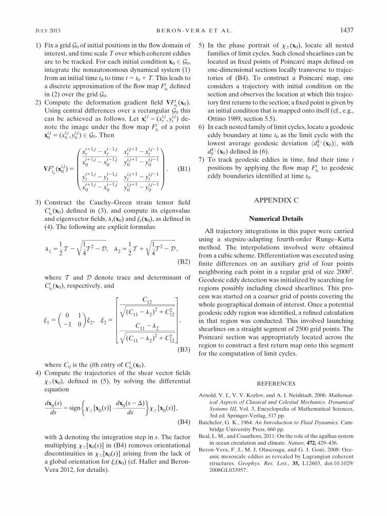
1) Fix a grid G0 of initial positions in the flow domain of

interest, and time scale T over which coherent eddies

are to be tracked. For each initial condition x0 2 G0,integrate the nonautonomous dynamical system (1)

from an initial time t0 to time t5 t01 T. This leads to

a discrete approximation of the flow map Ftt0defined

in (2) over the grid G0.2) Compute the deformation gradient field $Ft

t0(x0).

Using central differences over a rectangular G0 thiscan be achieved as follows. Let xi,jt 5 (x

i,jt , y

i,jt ) de-

note the image under the flow map Ftt0of a point

xi,j0 5 (xi,j0 , y

i,j0 ) 2 G0. Then

$Ftt0(x

i,j0 )5

0BBBBB@

xi11,jt 2 x

i21,jt

xi11,j0 2 x

i21,j0

xi,j11t 2 x

i,j21t

yi,j110 2 y

i,j210

yi11,jt 2 y

i21,jt

xi11,j0 2 x

i21,j0

yi,j11t 2 y

i,j21t

yi,j110 2 y

i,j210

1CCCCCA. (B1)

3) Construct the Cauchy–Green strain tensor field

Ctt0(x0) defined in (3), and compute its eigenvalue

and eigenvector fields, li(x0) and ji(x0), as defined in

(4). The following are explicit formulas:

l151

2T 2

ffiffiffiffiffiffiffiffiffiffiffiffiffiffiffiffiffiffi1

4T 22D

r, l25

1

2T 1

ffiffiffiffiffiffiffiffiffiffiffiffiffiffiffiffiffiffi1

4T 22D

r,

(B2)

where T and D denote trace and determinant of

Ctt0(x0), respectively, and

j15

�0 1

21 0

�j2, j25

26666664

C12ffiffiffiffiffiffiffiffiffiffiffiffiffiffiffiffiffiffiffiffiffiffiffiffiffiffiffiffiffiffiffiffiffiffiffiffiffi(C11 2 l2)

21C212

q

C11 2l2ffiffiffiffiffiffiffiffiffiffiffiffiffiffiffiffiffiffiffiffiffiffiffiffiffiffiffiffiffiffiffiffiffiffiffiffiffi(C11 2 l2)

21C212

q

37777775,

(B3)

where Cij is the ijth entry of Ctt0(x0).

4) Compute the trajectories of the shear vector fields

x6(x0), defined in (5), by solving the differential

equation

dx0(s)

ds5 sign

�x6[x0(s)] �

dx0(s2D)

ds

x6[x0(s)] ,

(B4)

with D denoting the integration step in s. The factor

multiplying x6[x0(s)] in (B4) removes orientational

discontinuities in x6[x0(s)] arising from the lack of

a global orientation for ji(x0) (cf. Haller and Beron-

Vera 2012, for details).

5) In the phase portrait of x6(x0), locate all nested

families of limit cycles. Such closed shearlines can be

located as fixed points of Poincar�e maps defined on

one-dimensional sections locally transverse to trajec-

tories of (B4). To construct a Poincar�e map, one

considers a trajectory with initial condition on the

section and observes the location at which this trajec-

tory first returns to the section; a fixed point is given by

an initial condition that is mapped onto itself (cf., e.g.,

Ottino 1989, section 5.5).

6) In each nested family of limit cycles, locate a geodesic

eddy boundary at time t0 as the limit cycle with the

lowest average geodesic deviation hdx6g (x0)i, with

dx6g (x0) defined in (6).

7) To track geodesic eddies in time, find their time t

positions by applying the flow map Ftt0to geodesic

eddy boundaries identified at time t0.

APPENDIX C

Numerical Details

All trajectory integrations in this paper were carried

using a stepsize-adapting fourth-order Runge–Kutta

method. The interpolations involved were obtained

from a cubic scheme. Differentiation was executed using

finite differences on an auxiliary grid of four points

neighboring each point in a regular grid of size 20002.

Geodesic eddy detection was initialized by searching for

regions possibly including closed shearlines. This pro-

cess was started on a coarser grid of points covering the

whole geographical domain of interest. Once a potential

geodesic eddy region was identified, a refined calculation

in that region was conducted. This involved launching

shearlines on a straight segment of 2500 grid points. The

Poincar�e section was appropriately located across the

region to construct a first return map onto this segment

for the computation of limit cycles.

REFERENCES

Arnold, V. I., V. V. Kozlov, and A. I. Neishtadt, 2006: Mathemat-

ical Aspects of Classical and Celestial Mechanics. Dynamical

Systems III, Vol. 3, Encyclopedia of Mathematical Sciences,

3rd ed. Springer-Verlag, 517 pp.

Batchelor, G. K., 1964: An Introduction to Fluid Dynamics. Cam-

bridge University Press, 660 pp.

Beal, L.M., and Coauthors, 2011: On the role of the agulhas system

in ocean circulation and climate. Nature, 472, 429–436.

Beron-Vera, F. J., M. J. Olascoaga, and G. J. Goni, 2008: Oce-

anic mesoscale eddies as revealed by Lagrangian coherent

structures. Geophys. Res. Lett., 35, L12603, doi:10.1029/

2008GL033957.


Biastoch, A., C. W. B€oning, J. R. E. Lutjeharms, and F. U.

Schwarzkopf, 2009: Increase in Agulhas leakage due to pole-

ward shift of the SouthernHemisphere westerlies.Nature, 462,

495–498.

Chelton, D. B., M. G. Schlax, R. M. Samelson, and R. A. de-

Szoeke, 2007: Global observations of large oceanic eddies.

Geophys. Res. Lett., 34, L15606, doi:10.1029/2007GL030812.

——, P. Gaube, M. G. Schlax, J. J. Early, and R. M. Samelson,

2011a: The influence of nonlinear mesoscale eddies on near-

surface oceanic chlorophyll. Science, 334, 328–332.

——, M. G. Schlax, and R. M. Samelson, 2011b: Global observa-

tions of nonlinear mesoscale eddies. Prog. Oceanogr., 91, 167–216.

Conti, C., D. Rossinelli, and P. Koumoutsakos, 2012: GPU and

APU computations of Finite Time Lyapunov Exponent fields.

J. Comput. Phys., 231, 2229–2244.

Doglioli, A. M., B. Blanke, S. Speich, and G. Lapeyre, 2007:

Tracking coherent structures in a regional ocean model with

wavelet analysis: Application to Cape Basin eddies. J. Geo-

phys. Res., 112, C05043, doi:10.1029/2006JC003952.

Early, J. J., R.M. Samelson, andD. B. Chelton, 2011: The evolution

and propagation of quasigeostrophic ocean eddies. J. Phys.

Oceanogr., 41, 1535–1555.Fang, F., and R. Morrow, 2003: Evolution, movement and decay of

warm-core Leeuwin Current eddies. Deep-Sea Res. II, 50,

2245–2261.

Froyland, G., C. Horenkamp, V. Rossi, N. Santitissadeekorn,

and A. S. Gupta, 2012: Three-dimensional characterization

and tracking of an Agulhas Ring. Ocean Modell., 52–53,

69–75.

Fu, L. L., D. B. Chelton, P.-Y. Le Traon, and R. Morrow, 2010:

Eddy dynamics from satellite altimetry.Oceanography (Wash.

D.C.), 23, 14–25.

Garth, C., F. Gerhardt, X. Tricoche, and H. Hans, 2007: Efficient

computation and visualization of coherent structures in fluid

flow applications. IEEE Trans. Visualization Computer

Graphics, 13, 1464–1471.Garzoli, S. L., P. L. Richardson, C. M. Duncombe Rae, D. M.

Fratantoni, G. J. Goni, and A. J. Roubicek, 1999: Three

Agulhas rings observed during the Benguela Current Exper-

iment. J. Geophys. Res., 20 (C9), 20 971–20 986.

Goni, G., and W. Johns, 2001: Census of warm rings and eddies in

the North Brazil Current retroflection region from 1992

through 1998 using TOPEX/Poseidon altimeter data. Geo-

phys. Res. Lett., 28, 1–4.Gordon, A., 1986: Inter-ocean exchange of thermocline water.

J. Geophys. Res., 91 (C4), 5037–5050.

Haller, G., 2001: Distinguished material surfaces and coherent

structures in 3D fluid flows. Physica D, 149, 248–277.——, 2005: An objective definition of a vortex. J. Fluid Mech., 525,

1–26.

——, and F. J. Beron-Vera, 2012: Geodesic theory of transport

barriers in two-dimensional flows. Physica D, 241, 1680–

1702.

Henson, S. A., and A. C. Thomas, 2008: A census of oceanic an-

ticyclonic eddies in the Gulf of Alaska. Deep-Sea Res. I, 55,

163–176.

Isern-Fontanet, J., E. Garc�ıa-Ladona, and J. Font, 2003: Iden-

tification of marine eddies from altimetric maps. J. Atmos.

Oceanic Technol., 20, 772–778.

Jorba, �A., and C. Sim�o, 1996: On quasi-periodic perturbations of

elliptic equilibrium points. SIAM J. Math. Anal., 27, 1704–1737.

Lehahn, Y., F. d’Ovidio, M. L�evy, Y. Amitai, and E. Heifetz, 2011:

Long range transport of a quasi isolated chlorophyll patch by

an Agulhas ring. Geophys. Res. Lett., 38, L16610, doi:10.1029/2011GL048588.

Le Traon, P.-Y., F. Nadal, and N. Ducet, 1998: An improved

mapping method of multisatellite altimeter data. J. Atmos.

Oceanic Technol., 15, 522–534.

Lugt, H. J., 1979: The dilemma of defining a vortex. Recent De-

velopments in Theoretical and Experimental Fluid Mechanics,

U. Muller, K. G. Riesner, and B. Schmidt, Eds., Springer-

Verlag, 309–321.

M�ezic, I., V. A. F. S. Loire, and P. Hogan, 2010: A new mixing

diagnostic and the Gulf of Mexico oil spill. Science, 330, 486.

Morrow, R., F. Birol, and D. Griffin, 2004: Divergent pathways of

cyclonic and anti-cyclonic ocean eddies. Geophys. Res. Lett.,

31, L24311, doi:10.1029/2004GL020974.

Okubo, A., 1970: Horizontal dispersion of flotable particles in the

vicinity of velocity singularity such as convergences.Deep-Sea

Res. Oceanogr. Abstr., 12, 445–454.

Olson, D., and R. Evans, 1986: Rings of the Agulhas Current.

Deep-Sea Res., 33, 27–42.Ottino, J., 1989: The Kinematics of Mixing: Stretching, Chaos and

Transport. Cambridge University Press, 364 pp.

Peacock, T., and J. Dabiri, 2010: Introduction to focus issue: La-

grangian coherent structures. Chaos, 20, 017501, doi:10.1063/1.3278173.

Ridgway, K. R., and J. R. Dunn, 2007: Observational evidence for

a Southern Hemisphere oceanic supergyre. Geophys. Res.

Lett., 34, L13612, doi:10.1029/2007GL030392.

Rio, M.-H., and F. Hernandez, 2004: A mean dynamic topography

computed over the world ocean from altimetry, in situ mea-

surements, and a geoid model. J. Geophys. Res., 109, C12032,doi:10.1029/2003JC002226.

Robinson, A. R., Ed., 1983: Eddies in Marine Science. Springer-

Verlag, 609 pp.

Souza, J. M. A. C., C. de Boyer Montegut, and P. Y. Le Traon,

2011: Comparison between three implementations of auto-

matic identification algorithms for the quantification and

characterization of mesoscale eddies in the South Atlantic

Ocean. Ocean Sci. Discuss., 8, 483–531.Turiel, A., J. Isern-Fontanet, and E. Garcia-Ladona, 2007:Wavelet

filtering to extract coherent vortices from altimetric data.

J. Atmos. Oceanic Technol., 24, 2103–2119.Weiss, J., 1991: The dynamics of enstrophy transfer in two-

dimensional hydrodynamics. Physica D, 48, 273–294.


objective detection of oceanic eddies and the agulhas...

Documents