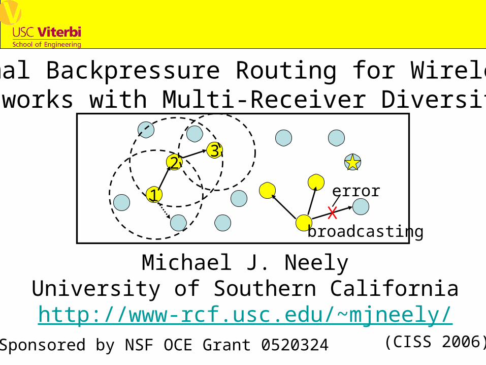
Optimal Backpressure Routing for Wireless Networks with Multi-Receiver Diversity

Michael J. NeelyUniversity of Southern Californiahttp://www-rcf.usc.edu/~mjneely/

*Sponsored by NSF OCE Grant 0520324 (CISS 2006)

1

23

broadcasting

error

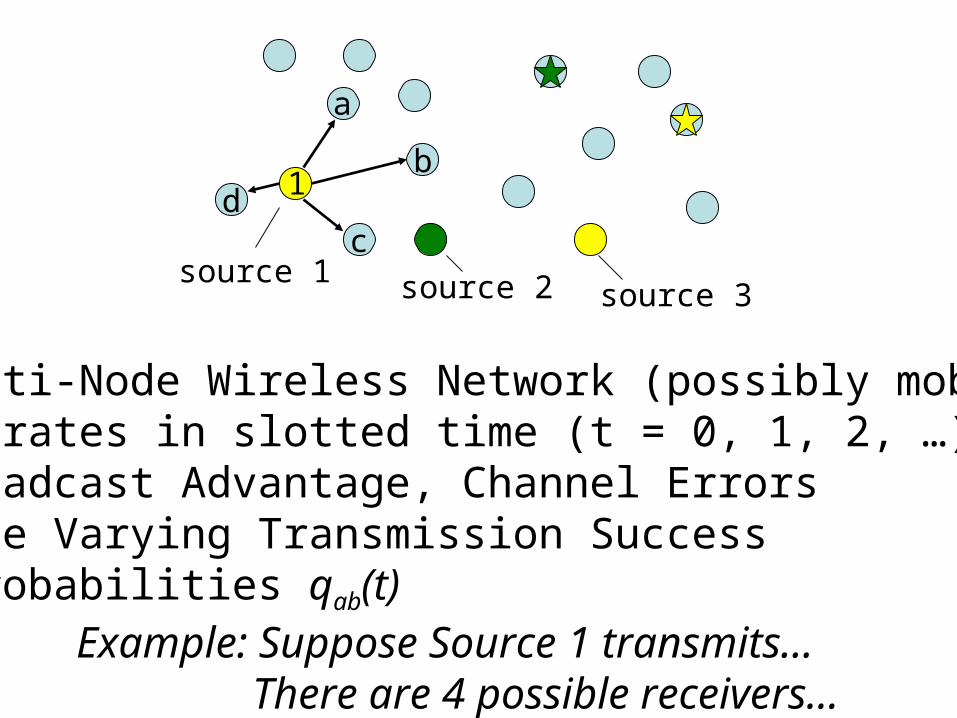
-Multi-Node Wireless Network (possibly mobile)-Operates in slotted time (t = 0, 1, 2, …)-Broadcast Advantage, Channel Errors-Time Varying Transmission Success Probabilities qab(t) Example: Suppose Source 1 transmits…

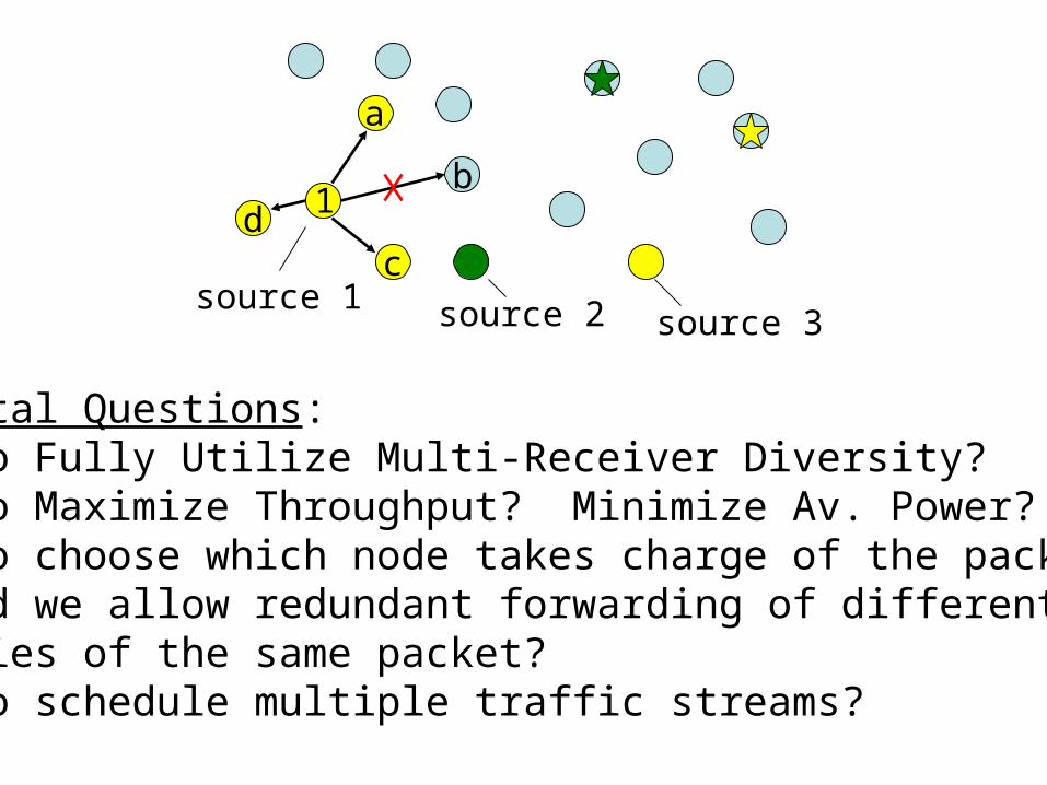
source 1 source 2 source 3

-Multi-Node Wireless Network (possibly mobile)-Operates in slotted time (t = 0, 1, 2, …)-Broadcast Advantage, Channel Errors-Time Varying Transmission Success Probabilities qab(t) Example: Suppose Source 1 transmits… There are 4 possible receivers…

db

csource 1 source 2 source 3

1

a

-Multi-Node Wireless Network (possibly mobile)-Operates in slotted time (t = 0, 1, 2, …)-Broadcast Advantage, Channel Errors-Time Varying Transmission Success Probabilities qab(t) Example: Suppose Source 1 transmits… Each with different success probs…

db

csource 1 source 2 source 3

1

a

db

csource 1 source 2 source 3

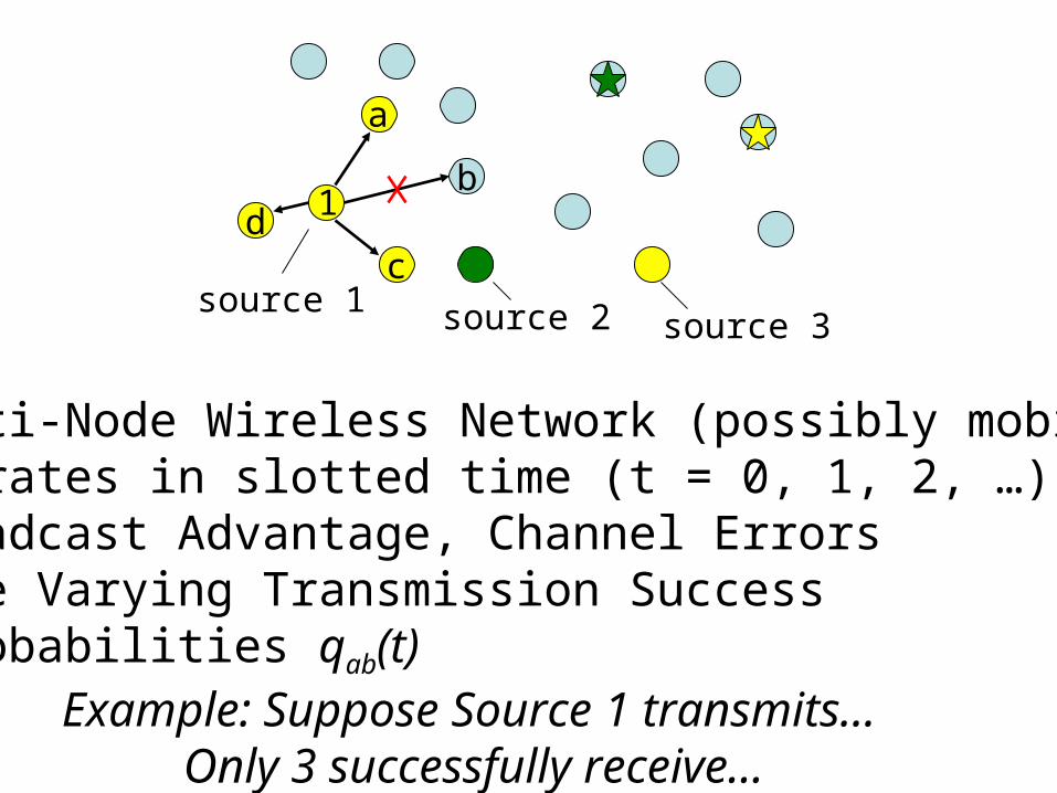
-Multi-Node Wireless Network (possibly mobile)-Operates in slotted time (t = 0, 1, 2, …)-Broadcast Advantage, Channel Errors-Time Varying Transmission Success Probabilities qab(t) Example: Suppose Source 1 transmits… Only 3 successfully receive…

1

a

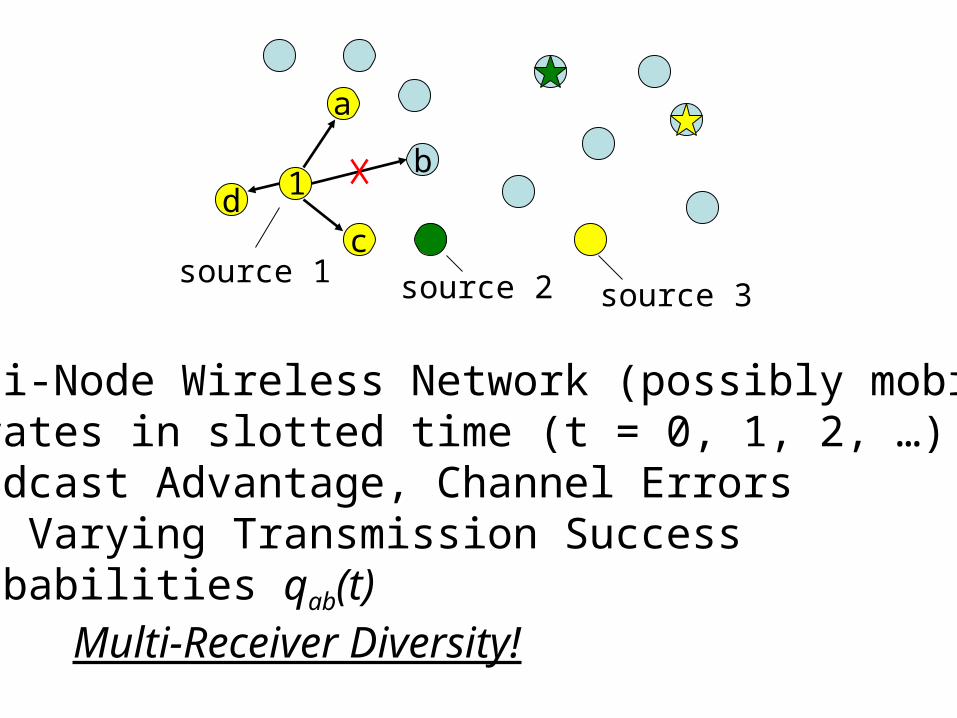
-Multi-Node Wireless Network (possibly mobile)-Operates in slotted time (t = 0, 1, 2, …)-Broadcast Advantage, Channel Errors-Time Varying Transmission Success Probabilities qab(t) Multi-Receiver Diversity!

db

csource 1 source 2 source 3

1

a

db

csource 1 source 2 source 3

1

a

Fundamental Questions: 1) How to Fully Utilize Multi-Receiver Diversity?2) How to Maximize Throughput? Minimize Av. Power?3) How to choose which node takes charge of the packet? 4) Should we allow redundant forwarding of different copies of the same packet? 5) How to schedule multiple traffic streams?

db

csource 1

1

a

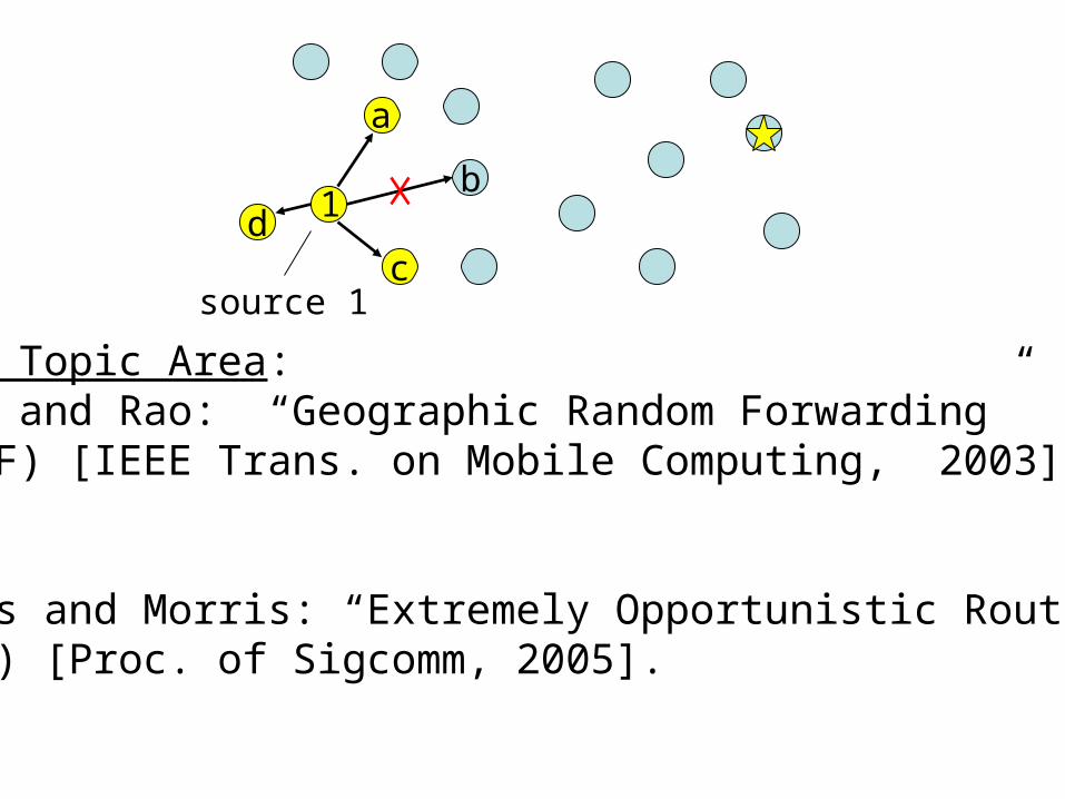
A Hot Topic Area: Zorzi and Rao: “Geographic Random Forwarding”(GeRaF) [IEEE Trans. on Mobile Computing, 2003].

Biswas and Morris: “Extremely Opportunistic Routing”(EXOR) [Proc. of Sigcomm, 2005].

db

csource 1

1

a

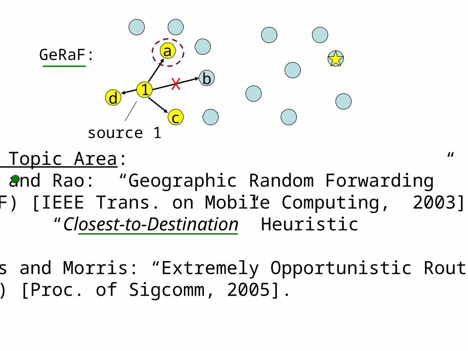
A Hot Topic Area: Zorzi and Rao: “Geographic Random Forwarding”(GeRaF) [IEEE Trans. on Mobile Computing, 2003]. “Closest-to-Destination” Heuristic

Biswas and Morris: “Extremely Opportunistic Routing”(EXOR) [Proc. of Sigcomm, 2005].

GeRaF:

1

23

Example of Deadlock Mode for Closest-to-DestinationRouting Heuristic:

Consistently send from 1--> 2 --> 3. But there are nonodes within transmission range of node 3 that are closer to the destination!

db

csource 1

1

a

A Hot Topic Area: Zorzi and Rao: “Geographic Random Forwarding”(GeRaF) [IEEE Trans. on Mobile Computing, 2003]. “Closest-to-Destination” Heuristic

Biswas and Morris: “Extremely Opportunistic Routing”(EXOR) [Proc. of Sigcomm, 2005].

“Fewest Expected Hops to Destination” Heuristic(using a traditional shortest path based on error probs)

h4h3

h5 h16h14

h11

h10

h15

h13

h12

h21

h1 h2

h17

h19

h23

h22

h18

h19h20

h25

h6

h9

h7 h1

h8

h24EXOR:

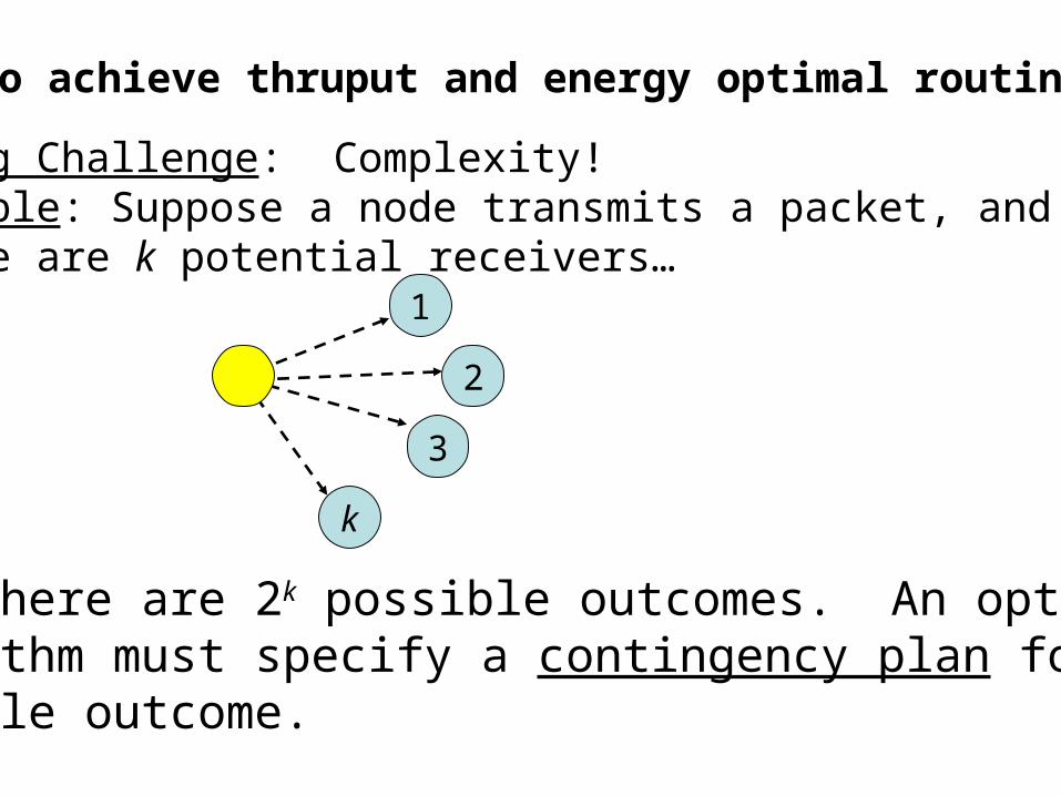
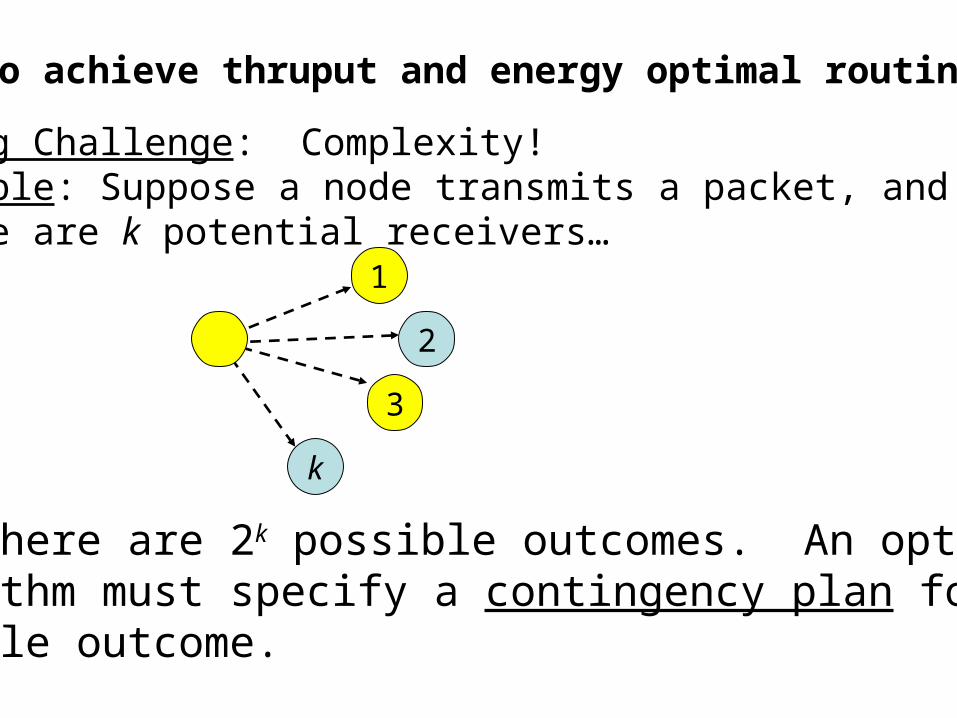
How to achieve thruput and energy optimal routing?

A Big Challenge: Complexity! Example: Suppose a node transmits a packet, andthere are k potential receivers…

1

2

3

k

Then there are 2k possible outcomes. An optimalalgorithm must specify a contingency plan for eachpossible outcome.

A Big Challenge: Complexity! Example: Suppose a node transmits a packet, andthere are k potential receivers…

1

2

3

k

Then there are 2k possible outcomes. An optimalalgorithm must specify a contingency plan for eachpossible outcome.

How to achieve thruput and energy optimal routing?

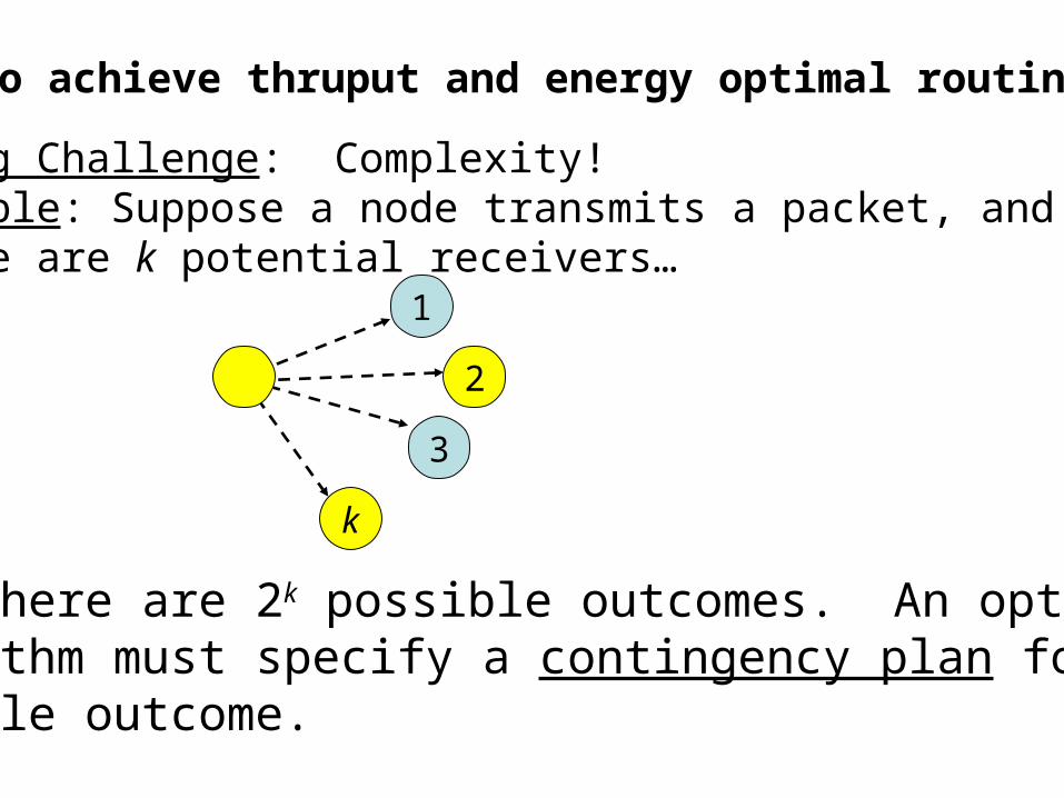
A Big Challenge: Complexity! Example: Suppose a node transmits a packet, andthere are k potential receivers…

1

2

3

k

Then there are 2k possible outcomes. An optimalalgorithm must specify a contingency plan for eachpossible outcome.

How to achieve thruput and energy optimal routing?

A Big Challenge: Complexity! Example: Suppose a node transmits a packet, andthere are k potential receivers…

1

2

3

k

Then there are 2k possible outcomes. An optimalalgorithm must specify a contingency plan for eachpossible outcome.

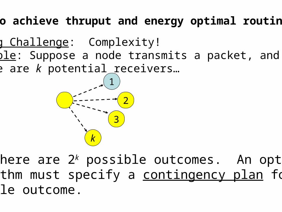
How to achieve thruput and energy optimal routing?

A Big Challenge: Complexity! Example: Suppose a node transmits a packet, andthere are k potential receivers…

1

2

3

k

Then there are 2k possible outcomes. An optimalalgorithm must specify a contingency plan for eachpossible outcome.

How to achieve thruput and energy optimal routing?

A Big Challenge: Complexity! Example: Suppose a node transmits a packet, andthere are k potential receivers…

1

2

3

k

Then there are 2k possible outcomes. An optimalalgorithm must specify a contingency plan for eachpossible outcome.

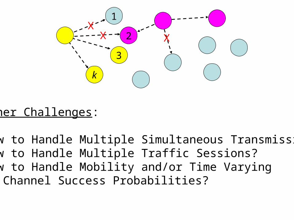
How to achieve thruput and energy optimal routing?

1

2

3

k

Further Challenges:

1) How to Handle Multiple Simultaneous Transmissions?2) How to Handle Multiple Traffic Sessions? 3) How to Handle Mobility and/or Time Varying Channel Success Probabilities?

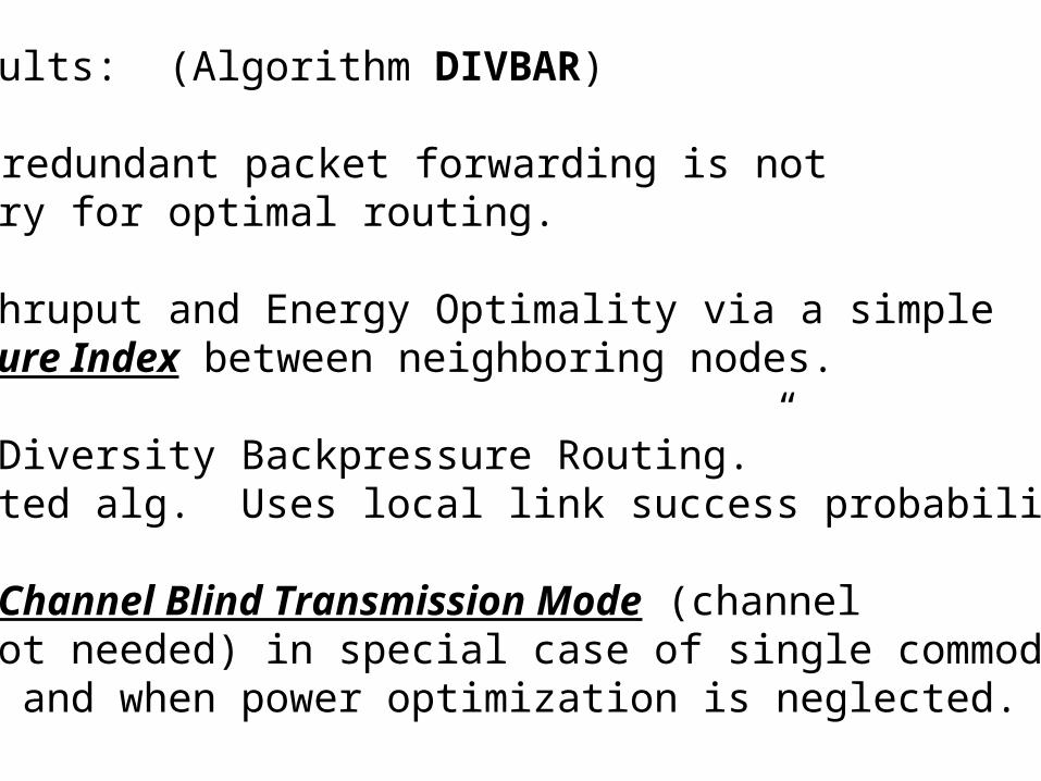
Our Main Results: (Algorithm DIVBAR)

1. Show that redundant packet forwarding is not necessary for optimal routing.

2. Achieve Thruput and Energy Optimality via a simple Backpressure Index between neighboring nodes.

3. DIVBAR: “Diversity Backpressure Routing.” Distributed alg. Uses local link success probability info.

4. Admits a Channel Blind Transmission Mode (channel probs. not needed) in special case of single commodity networks and when power optimization is neglected.

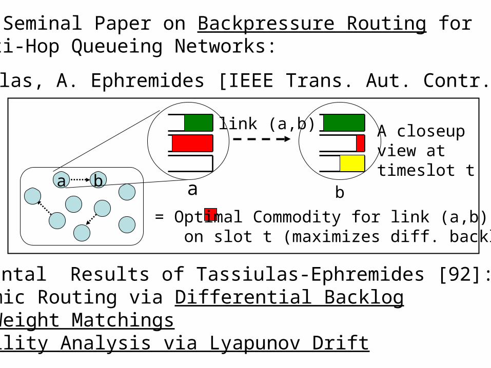
The Seminal Paper on Backpressure Routing for Multi-Hop Queueing Networks:

L. Tassiulas, A. Ephremides [IEEE Trans. Aut. Contr. 1992]

Fundamental Results of Tassiulas-Ephremides [92]: a. Dynamic Routing via Differential Backlogb. Max Weight Matchingsc. Stability Analysis via Lyapunov Drift

link (a,b)

a b a b

= Optimal Commodity for link (a,b) on slot t (maximizes diff. backlog)

A closeupview at timeslot t

A brief history of Lyapunov Drift for Queueing Systems:Lyapunov Stability: Tassiulas, Ephremides [91, 92, 93] P. R. Kumar, S. Meyn [95]McKeown, Anantharam, Walrand [96, 99]Kahale, P. E. Wright [97]Andrews, Kumaran, Ramanan, Stolyar, Whiting [2001]Leonardi, Melia, Neri, Marsan [2001]Neely, Modiano, Rohrs [2002, 2003, 2005]

Lyapunov Stability with Stochastic Performance Optimization:Neely, Modiano [2003, 2005] (Fairness, Energy)Georgiadis, Neely, Tassiulas [NOW Publishers, F&T, 2006]

Alternate Approaches to Stoch. Performance Optimization:Eryilmaz, Srikant [2005] (Fluid Model Transformations)Stolyar [2005] (Fluid Model Transformations)Lee, Mazumdar, Shroff [2005] (Stochastic Gradients)

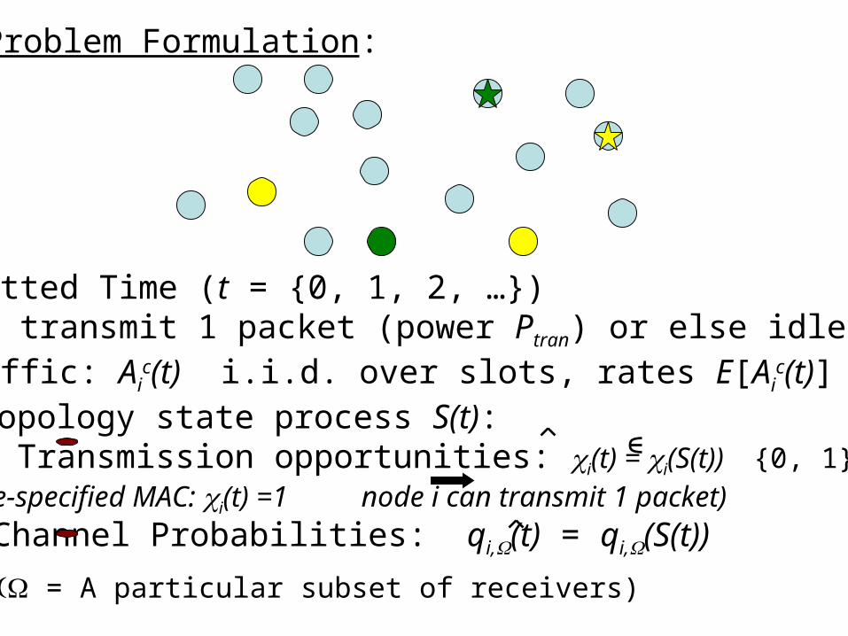
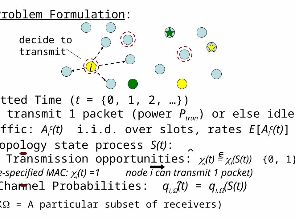
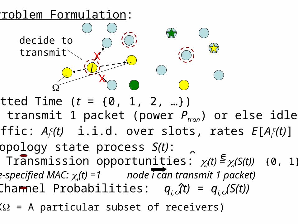
Problem Formulation:

1. Slotted Time (t = {0, 1, 2, …})2. Can transmit 1 packet (power Ptran) or else idle. 3. Traffic: Ai

c(t) i.i.d. over slots, rates E[Aic(t)] = i

c

4. Topology state process S(t): Transmission opportunities: i(t) = i(S(t)) {0, 1} (Pre-specified MAC: i(t) =1 node i can transmit 1 packet)

Channel Probabilities: qi,(t) = qi,(S(t))

= A particular subset of receivers)

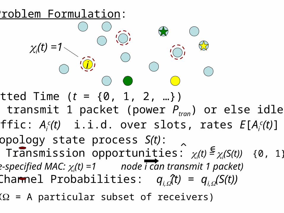
i

i(t) =1

Problem Formulation:

1. Slotted Time (t = {0, 1, 2, …})2. Can transmit 1 packet (power Ptran) or else idle. 3. Traffic: Ai

c(t) i.i.d. over slots, rates E[Aic(t)] = i

c

4. Topology state process S(t): Transmission opportunities: i(t) = i(S(t)) {0, 1} (Pre-specified MAC: i(t) =1 node i can transmit 1 packet)

Channel Probabilities: qi,(t) = qi,(S(t))

= A particular subset of receivers)

i

decide totransmit

Problem Formulation:

1. Slotted Time (t = {0, 1, 2, …})2. Can transmit 1 packet (power Ptran) or else idle. 3. Traffic: Ai

c(t) i.i.d. over slots, rates E[Aic(t)] = i

c

4. Topology state process S(t): Transmission opportunities: i(t) = i(S(t)) {0, 1} (Pre-specified MAC: i(t) =1 node i can transmit 1 packet)

Channel Probabilities: qi,(t) = qi,(S(t))

= A particular subset of receivers)

Problem Formulation:

i

decide totransmit

1. Slotted Time (t = {0, 1, 2, …})2. Can transmit 1 packet (power Ptran) or else idle. 3. Traffic: Ai

c(t) i.i.d. over slots, rates E[Aic(t)] = i

c

4. Topology state process S(t): Transmission opportunities: i(t) = i(S(t)) {0, 1} (Pre-specified MAC: i(t) =1 node i can transmit 1 packet)

Channel Probabilities: qi,(t) = qi,(S(t))

= A particular subset of receivers)

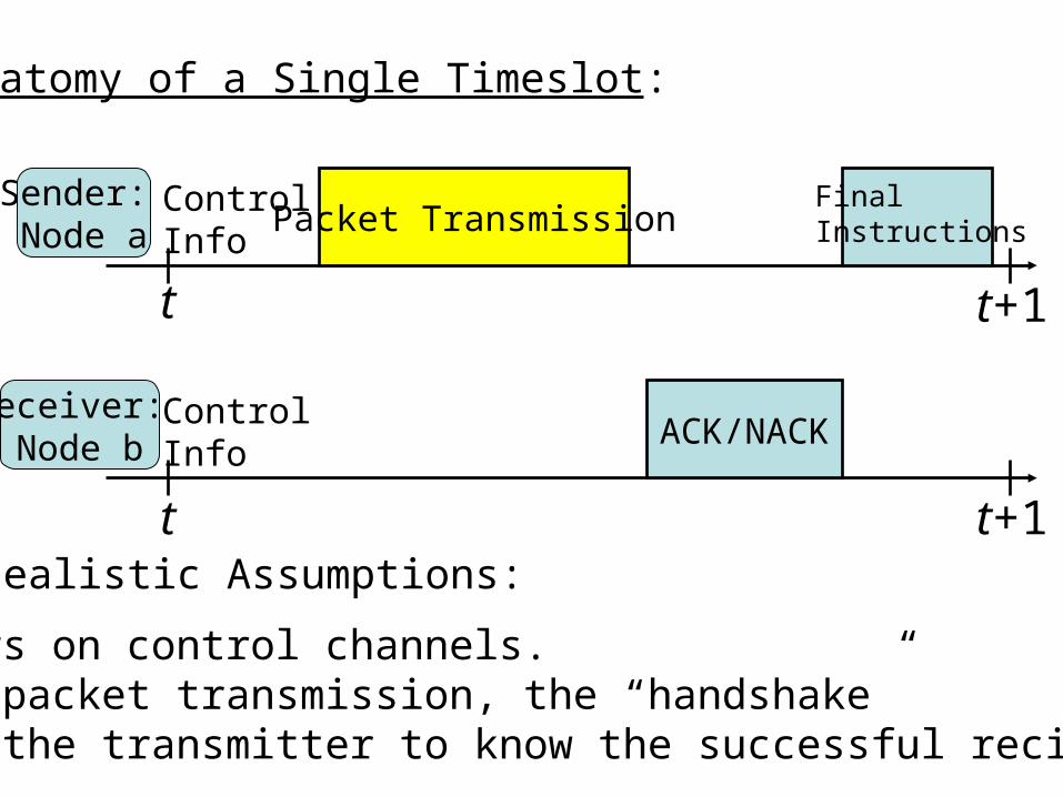
Anatomy of a Single Timeslot:

Receiver: Node b

Packet TransmissionSender: Node a

ControlInfo

FinalInstructions

ControlInfo

t+1t

t+1t

ACK/NACK

-No errors on control channels.-After a packet transmission, the “handshake” enables the transmitter to know the successful recipients.

Idealistic Assumptions:

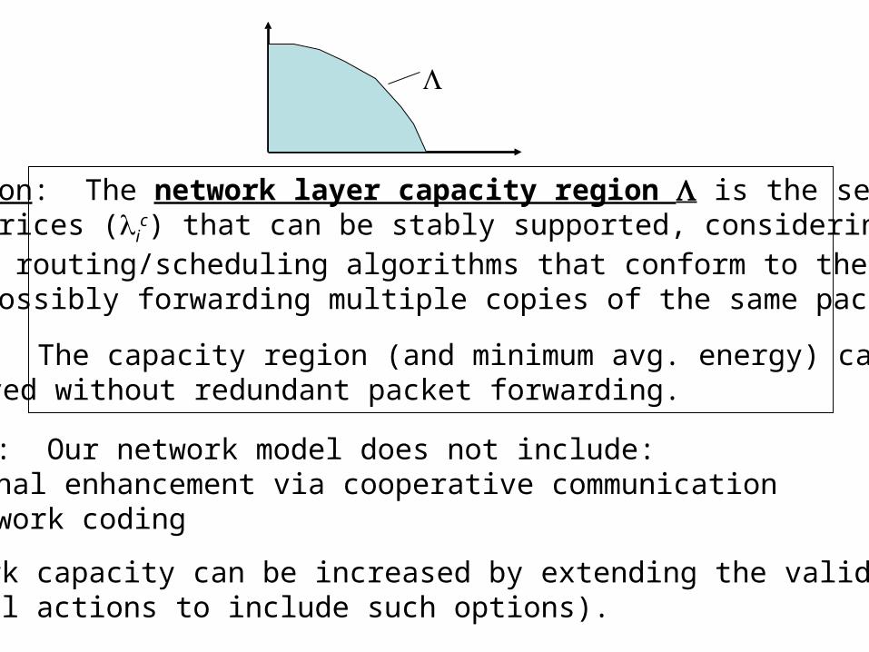
Definition: The network layer capacity region is the set of allrate matrices (i

c) that can be stably supported, considering all possible routing/scheduling algorithms that conform to the networkmodel (possibly forwarding multiple copies of the same packet).

Note: Our network model does not include: -Signal enhancement via cooperative communication-Network coding

(Network capacity can be increased by extending the valid control actions to include such options).

Lemma: The capacity region (and minimum avg. energy) can beachieved without redundant packet forwarding.

Theorem 1: (Network Capacity and Minimum Avg. Energy)(a) Network Capacity Region is given by all (i

c) such that:

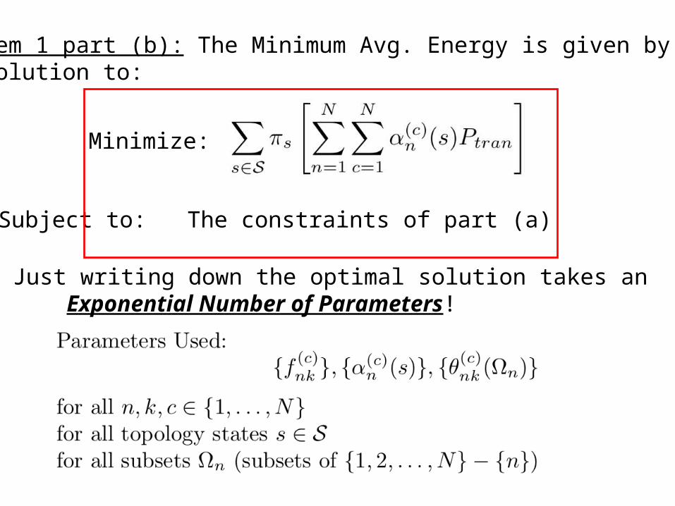
Theorem 1 part (b): The Minimum Avg. Energy is given by the solution to:

Minimize:

Subject to: The constraints of part (a)

Note: Just writing down the optimal solution takes an Exponential Number of Parameters!

Theorem 1 part (b): The Minimum Avg. Energy is given by the solution to:

Minimize:

Subject to: The constraints of part (a)

Note: Just writing down the optimal solution takes an Exponential Number of Parameters!

A Simple Backpressure Solution (in terms of a control parameter V):Algorithm DIVBAR “Diversity Backpressure Routing”

Let n(t) = 1

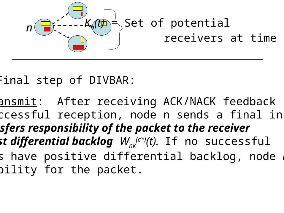
Kn(t) = Set of potential receivers at time t.

n

1. For each k Kn(t), compute Wnk(c)(t):

Wnk(c)(t) = max[Un

(c)(t) - Uk(c)(t), 0]

(Differential Backlog)

(Uk(c)(t)=# commodity c packets in node n at slot t)

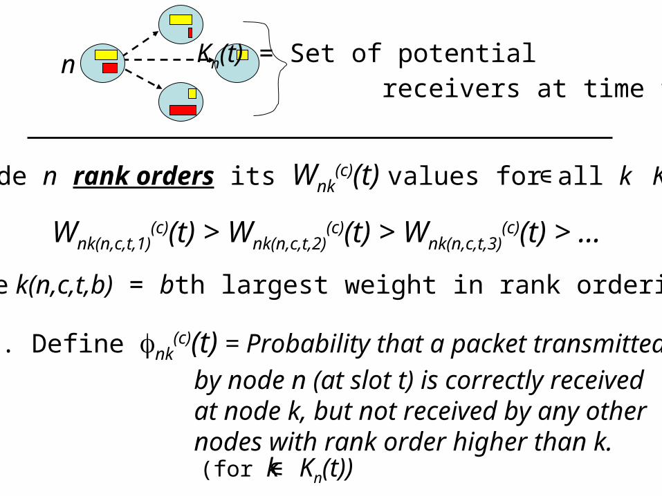
n Kn(t) = Set of potential receivers at time t.

2. Node n rank orders its Wnk(c)(t) values for all k Kn(t):

Wnk(n,c,t,1)(c)(t) > Wnk(n,c,t,2)

(c)(t) > Wnk(n,c,t,3)(c)(t) > …

(where k(n,c,t,b) = bth largest weight in rank ordering)

3. Define nk(c)(t) = Probability that a packet transmitted

by node n (at slot t) is correctly received at node k, but not received by any other nodes with rank order higher than k.

(for k Kn(t))

n Kn(t) = Set of potential receivers at time t.

4. Define the optimal commodity c*n(t) as the maximizer of:

Define Wn*(t) as the above maximum weighted sum.

5. If Wn*(t) > V Ptran then transmit a packet of commodity c*n(t) . Else, remain idle.

n Kn(t) = Set of potential receivers at time t.

Final step of DIVBAR:

If we transmit: After receiving ACK/NACK feedback about successful reception, node n sends a final instruction that transfers responsibility of the packet to the receiver with largest differential backlog Wnk

(c*)(t). If no successfulreceivers have positive differential backlog, node n retainsresponsibility for the packet.

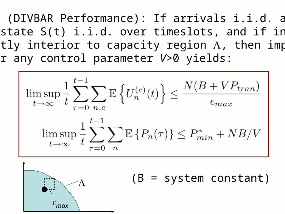
Theorem 2 (DIVBAR Performance): If arrivals i.i.d. and topology state S(t) i.i.d. over timeslots, and if input ratesare strictly interior to capacity region , then implementingDIVBAR for any control parameter V>0 yields:

max

(B = system constant)

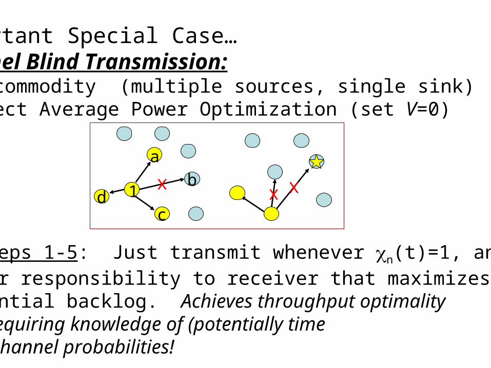
Important Special Case…Channel Blind Transmission:-One commodity (multiple sources, single sink)-Neglect Average Power Optimization (set V=0)

db

c

1

a

Skip steps 1-5: Just transmit whenever n(t)=1, and transfer responsibility to receiver that maximizes differential backlog. Achieves throughput optimalitywithout requiring knowledge of (potentially time varying) channel probabilities!

Extensions: -Variable Rate and Power Control-Optimizing the MAC layer

(t)=(1(t), 2(t), …, N(t)) (# packets transmitted)P(t) = (P1(t), P2(t), …, PN(t)) (Power allocation vector)

I(t) = ((t); P(t)) = Collective Control Action

qn, Wn(t) = qn, Wn(I(t), S(t))

Jointly choose I(t), cn*(t) to maximize:

DIVBAR can easily be integrated with other cross-layerperformance objectives using stochastic Lyapunov optimization,using techniques of Virtual Power Queues, Auxiliary Variables, Flow State Queues developed in:

-Fairness, Flow Control for inside or outside of capacity region [Neely thesis 2003, Neely, Modiano, Li Infocom 2005]

-Energy Constraints, General Functions of Energy [Neely Infocom 2005] [Georgiadis, Neely, Tassiulas NOW 2006]

Flow control reservoir

DIVBAR also works for: -Non-i.i.d. arrivals and channel states-“Enhanced DIVBAR” (EDR) (improve delay via shortest path metric)-Distributed MAC via Random Access(similar to analysis in Neely 2003, JSAC 2005)

(DRPCAlg. OfJSAC 2005)

The “cost” of adistributed MACfor DRPC (withoutmulti-receiver diversity)

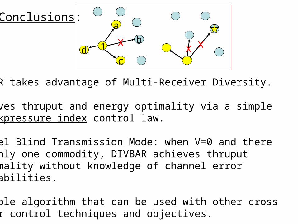
1. DIVBAR takes advantage of Multi-Receiver Diversity.

2. Achieves thruput and energy optimality via a simple backpressure index control law.

3. Channel Blind Transmission Mode: when V=0 and there is only one commodity, DIVBAR achieves thruput optimality without knowledge of channel error probabilities.

4. Flexible algorithm that can be used with other cross layer control techniques and objectives.

db

c

1

aConclusions: